University of South CarolinaScholar Commons

Theses and Dissertations

2017

Functional Data Smoothing Methods and TheirApplicationsSongqiao HuangUniversity of South Carolina

Follow this and additional works at: https://scholarcommons.sc.edu/etd

Part of the Statistics and Probability Commons

This Open Access Dissertation is brought to you by Scholar Commons. It has been accepted for inclusion in Theses and Dissertations by an authorizedadministrator of Scholar Commons. For more information, please contact dillarda@mailbox.sc.edu.

Recommended CitationHuang, S.(2017). Functional Data Smoothing Methods and Their Applications. (Doctoral dissertation). Retrieved fromhttps://scholarcommons.sc.edu/etd/4345

Functional Data Smoothing Methods and Their Applications

by

Songqiao Huang

Bachelor of ScienceBinghamton University, State University of New York, 2011

Submitted in Partial Fulfillment of the Requirements

for the Degree of Doctor of Philosophy in

Statistics

College of Arts and Sciences

University of South Carolina

2017

Accepted by:

David B. Hitchcock, Major Professor

Paramita Chakraborty, Committee Member

Xiaoyan Lin, Committee Member

Susan E. Steck, Committee Member

Cheryl L. Addy, Vice Provost and Dean of the Graduate School

c© Copyright by Songqiao Huang, 2017All Rights Reserved.

ii

Dedication

To my parents Jingmin Huang and Chunhua Xu, grandparents Xishen Xu and

Caiyun Jiao, Yanshan Huang and Youlian Gao, and husband Peijie Hou, you are

always there with me whenever and wherever I am.

iii

Acknowledgments

I want to express my greatest gratitude to my academic advisor, Dr. David B. Hitch-

cock, who has encouraged, inspired, motivated me, and guided me through all the

obstacles in my Ph.D. study with great patience. Dr. Hitchcock is not only my aca-

demic advisor, but is also a very good life mentor and friend. His knowledge, patience

and carefulness toward research, and his great advice and encouragements for other

aspects of life during my years at the University of South Carolina, Columbia have

helped me grow and become stronger both academically and personally.

I also want to thank all of my committee members, Dr. Susan Steck, Dr. Paramita

Chakraborty and Dr. Xiaoyan Lin for carefully reviewing my dissertation, and for

their insightful suggestions and comments on my dissertation.

Above all, I want to thank the most important persons in my life: My parents

Jingmin Huang and Chunhua Xu, my grandparents Xishen Xu, Caiyun Jiao, and

Yanshan Huang, and my husband Peijie Hou. Without their unconditional love, con-

sistent support and encouragements, I couldn’t have grown to be the person I am

today.

iv

Abstract

In many subjects such as psychology, geography, physiology or behavioral science,

researchers collect and analyze non-traditional data, i.e., data that do not consist of

a set of scalar or vector observations, but rather a set of sequential observations mea-

sured over a fine grid on a continuous domain, such as time, space, etc. Because the

underlying functional structure of the individual datum is of interest, Ramsay and

Dalzell (1991) named the collection of topics involving analyzing these functional ob-

servations functional data analysis (FDA). Topics in functional data analysis include

data smoothing, data registration, regression analysis with functional responses, clus-

ter analysis on functional data, etc. Among these topics, data smoothing and data

registration serve as preliminary steps that allow for more reliable statistical inference

afterwards. In this dissertation, we include three research projects on functional data

smoothing and its effects on functional data applications. In particular, Chapter 2

mainly presents a unified Bayesian approach that borrows the idea of time warping

to represent functional curves of various shapes. Based on a comparison with the

method of B-splines developed by de Boor (2001) and some other methods that are

well known for its broad applications in curve fitting, our method is proved to adapt

more flexibly to highly irregular curves. Then, Chapter 3 discusses subsequent re-

gression and clustering methods for functional data, and investigates the accuracy of

functional regression prediction as well as clustering results as measured by either tra-

ditional in-sample and out-of-sample sum of squares or the Rand index. It is showed

that using our Bayesian smoothing method on the raw curves prior to carrying out

the corresponding applications provides very competitive statistical inference and an-

v

alytic results in most scenarios compared to using other standard smoothing methods

prior to the applications. Lastly, notice that one restriction for our method in Chap-

ter 2 is that it can only be applied to functional curves that are observed on a fine

grid of time points. Hence, in Chapter 4, we extend the idea of our transformed basis

smoothing method in Chapter 2 to the sparse functional data scenario. We show via

simulations and analysis that the proposed method gives a very good approximation

of the overall pattern as well as the individual trends for the data with the cluster of

sparsely observed curves.

vi

Table of Contents

Dedication . . . . . . . . . . . . . . . . . . . . . . . . . . . . . . . . . . iii

Acknowledgments . . . . . . . . . . . . . . . . . . . . . . . . . . . . . iv

Abstract . . . . . . . . . . . . . . . . . . . . . . . . . . . . . . . . . . . v

List of Tables . . . . . . . . . . . . . . . . . . . . . . . . . . . . . . . . ix

List of Figures . . . . . . . . . . . . . . . . . . . . . . . . . . . . . . . xi

Chapter 1 Introduction . . . . . . . . . . . . . . . . . . . . . . . . . 1

1.1 Literature Review . . . . . . . . . . . . . . . . . . . . . . . . . . . . . 1

1.2 Outline . . . . . . . . . . . . . . . . . . . . . . . . . . . . . . . . . . . 7

Chapter 2 Bayesian functional data fitting with transformedB-splines . . . . . . . . . . . . . . . . . . . . . . . . . . . 9

2.1 Introduction . . . . . . . . . . . . . . . . . . . . . . . . . . . . . . . . 10

2.2 Review of Concepts . . . . . . . . . . . . . . . . . . . . . . . . . . . . 12

2.3 Bayesian Model Fitting for Functional Curves . . . . . . . . . . . . . 16

2.4 Knot Selection with Reversible Jump MCMC . . . . . . . . . . . . . 27

2.5 Simulation Studies . . . . . . . . . . . . . . . . . . . . . . . . . . . . 31

2.6 Real Data Application . . . . . . . . . . . . . . . . . . . . . . . . . . 38

2.7 Discussion . . . . . . . . . . . . . . . . . . . . . . . . . . . . . . . . . 41

vii

Chapter 3 Functional regression and clustering with func-tional data smoothing . . . . . . . . . . . . . . . . . . . 42

3.1 Introduction . . . . . . . . . . . . . . . . . . . . . . . . . . . . . . . . 42

3.2 Simulation Studies: Functional Clustering . . . . . . . . . . . . . . . 45

3.3 Simulation Studies: Functional Regression . . . . . . . . . . . . . . . 48

3.4 Real Data Application: Functional Regression Example 1 . . . . . . . 57

3.5 Real Data Application: Functional Regression Example 2 . . . . . . . 62

3.6 Discussion . . . . . . . . . . . . . . . . . . . . . . . . . . . . . . . . . 83

Chapter 4 Sparse functional data fitting with transformedspline basis . . . . . . . . . . . . . . . . . . . . . . . . . . 86

4.1 Introduction . . . . . . . . . . . . . . . . . . . . . . . . . . . . . . . . 86

4.2 Bayesian Model Fitting for Sparse Functional Curves . . . . . . . . . 89

4.3 Simulation Studies . . . . . . . . . . . . . . . . . . . . . . . . . . . . 104

4.4 Discussion . . . . . . . . . . . . . . . . . . . . . . . . . . . . . . . . . 109

Chapter 5 Conclusion . . . . . . . . . . . . . . . . . . . . . . . . . . 113

Bibliography . . . . . . . . . . . . . . . . . . . . . . . . . . . . . . . . 116

viii

List of Tables

Table 2.1 MSE comparison table for five smoothing methods. Top: MSEvalues calculated with respect to the observed curve. Bottom:MSE values calculated with respect to the true signal curve. . . . . 37

Table 2.2 MSE comparison table for six smoothing methods. Digits in theWeights column represent the weighting of the simulated peri-odic curve, smooth curve and spiky curve, respectively. Top rowin each cell: MSE value calculated with respect to the observedcurve. Bottom row in each cell: MSE value calculated with re-spect to the true signal curve. . . . . . . . . . . . . . . . . . . . . 38

Table 3.1 Rand index values for five smoothing methods based on regulardistance matrix . . . . . . . . . . . . . . . . . . . . . . . . . . . . 47

Table 3.2 Rand index values for five smoothing methods based on stan-dardized distance matrix . . . . . . . . . . . . . . . . . . . . . . . 47

Table 3.3 In-sample SSE comparison for functional regression predictionsbased on simulated curves . . . . . . . . . . . . . . . . . . . . . . . 50

Table 3.4 Out-of-sample SSE comparison for functional regression predic-tions based on simulated curves . . . . . . . . . . . . . . . . . . . 55

Table 3.5 SSE comparison table: Model 1: both dew point and humidityare predictors. Top: SSE for predicted response curves with re-spect to the true observed curve, no further smoothing on α1(t),β11(t) and β12(t). Bottom: SSE for predicted response curveswith respect to the true signal curve, with further smoothing onα1(t), β11(t) and β12(t) using regular B-spline basis functions. . . . 58

Table 3.6 In-sample SSE comparison: Model 2: dew point is the only pre-dictor. Top: SSE for predicted response curves with respect tothe true signal curve, no further smoothing on α2(t) and β1(t).Bottom: SSE for predicted response curves with respect to thetrue observed curve, with further smoothing on α2(t) and β1(t)using regular B-splines basis functions. . . . . . . . . . . . . . . . . 58

ix

Table 3.7 In-sample SSE comparison: Model 3: humidity is the only pre-dictor. Top: SSE for predicted response curves with respect tothe true signal curve, no further smoothing on α3(t) and β2(t).Bottom: SSE for predicted response curves with respect to thetrue observed curve, with further smoothing on α3(t) and β2(t)using regular B-splines basis functions. . . . . . . . . . . . . . . . . 61

Table 3.8 SSE comparison for seven flood events. Top: SSE values basedon functional regression without any smoothing. Bottom: SSEvalues based on functional regression with raw data curves andestimated intercept and slope curves smoothed via smoothing splines. 68

Table 3.9 SSE comparison for seven flood events. SSE values based onfunctional regression without any pre-smoothing on the obser-vation curves. “Cross-validation” idea is utilized to obtain out-of-sample predictions. Top: SSE values based on functional re-gression without any smoothing. Bottom: SSE values based onfunctional regression with raw data curves and estimated inter-cept and slope curves smoothed via smoothing splines. . . . . . . . 72

Table 3.10 SSE comparison for seven flood events. SSE values based onfunctional regression with Bayesian transformed B-splines methodon the observed curves. . . . . . . . . . . . . . . . . . . . . . . . . 73

Table 3.11 SSE comparison for seven flood events. SSE values based onfunctional regression with Bayesian transformed B-splines methodon the observation curves. Top: No further smoothing on α(t)and β(t) curves. Middle: α(t) and β(t) curves further smoothedusing smoothed splines with roughness parameter = 0.9. Bot-tom: α(t) and β(t) curves further smoothed using smoothedsplines with roughness parameter = 0.5. . . . . . . . . . . . . . . . 77

Table 3.12 SSE comparison for seven flood events. SSE values based onfunctional regression with Bayesian transformed B-splines methodon the observation curves. “Cross-validation” idea is utilized toobtain out-of-sample predictions. Top: No further smoothingon α(t) and β(t) curves. Bottom: α(t) and β(t) curves furthersmoothed using smoothed splines with roughness parameter = 0.9. 82

x

List of Figures

Figure 2.1 Comparison plot of two normal density curves. Dashed curve:density of N(0, σ2

di+c2

i ζ2i ). Solid curve: density of N(0, σ2

di+ζ2

i ).(ci, σdi/ζi) = (5, 1). . . . . . . . . . . . . . . . . . . . . . . . . . . 20

Figure 2.2 Comparison plot of two normal density curves. Dashed curve:density of N(0, σ2

di+c2

i ζ2i ). Solid curve: density of N(0, σ2

di+ζ2

i ).(ci, σdi/ζi) = (100, 10). . . . . . . . . . . . . . . . . . . . . . . . . 20

Figure 2.3 True versus fitted simulated curves. Dashed spiky curve: sim-ulated true signal curve. Solid wiggly curve: correspondingobserved curve. . . . . . . . . . . . . . . . . . . . . . . . . . . . . 33

Figure 2.4 Mean squared error trace plot of 1000 MCMC iterations . . . . . 34

Figure 2.5 Example of set of 15 transformed B-splines obtained from oneMCMC iteration . . . . . . . . . . . . . . . . . . . . . . . . . . . 34

Figure 2.6 True signal curve versus fitted curves from three competingmethods. Black solid curve: true signal curve. Red dashedcurve: fitted curve obtained from Bayesian transformed B-splinesmethod. Blue dotted curve: fitted curve obtained from B-splines basis functions. Dashed green curve: fitted curve ob-tained from B-splines basis functions with selected knots. . . . . . 35

Figure 2.7 True signal curve versus fitted curves from three competingmethods. Black solid curve: true signal curve. Red dashedcurve: fitted curve obtained from Bayesian transformed B-splinesmethod. Blue dotted curve: fitted curve obtained from thewavelet basis functions. Dashed green curve: fitted curve ob-tained from the Fourier basis functions. . . . . . . . . . . . . . . . 36

Figure 2.8 Observed versus smoothed wind speed curves. Top: four ob-served wind speed curves. Bottom: four corresponding windspeed curves smoothed with Bayesian transformed B-splines ba-sis functions. . . . . . . . . . . . . . . . . . . . . . . . . . . . . . 39

xi

Figure 2.9 Side by side boxplots of MSE values for five smoothing meth-ods. From left to right: boxplot of MSE values for 18 oceanwind curves smoothed with the selected knots B-splines (SKB);the B-splines with equally selected knots (B); the Wavelet basis(Wave); the Fourier basis (Fourier) and the Bayesian trans-formed B-splines (TB). . . . . . . . . . . . . . . . . . . . . . . . . 40

Figure 3.1 Simulated curves from four clusters. . . . . . . . . . . . . . . . . . 46

Figure 3.2 Boxplots of SSE values for the first 9 predicted response curveswith no presmoothing or presmoothing using the transformedB-splines, the Fourier basis, the Wavelet basis and regular B-splines basis functions on the curves. Red line: SSE value forthe predicted response curves with presmoothing on the curvesusing the transformed B-splines. . . . . . . . . . . . . . . . . . . . 52

Figure 3.3 The first 9 predicted response curves. Black spiky curves: truesignal response curves. Red long dashed curves: predictedcurves with presmoothing using the transformed B-splines. Pur-ple wiggly curves: predicted response curves with no presmooth-ing on the curves. Green dashed curve: predicted responsecurves with presmoothing using the Fourier basis functions. . . . 53

Figure 3.4 The first 9 predicted response curves. Black spiky curves: truesignal response curves. Red long dashed curves: predictedcurves with presmoothing using the transformed B-splines. Bluewiggly curves: predicted response curves with with presmooth-ing using the Wavelet basis functions. Green dashed curve:predicted response curves with presmoothing using the regularB-spline basis functions. . . . . . . . . . . . . . . . . . . . . . . . 54

Figure 3.5 True Orlando temperature curves and predicted response curveswithout data smoothing, or with data presmoothed using thetransformed B-spline basis and the Fourier basis functions. Blacksolid curve: true Orlando weather curves. Green solid curve:predicted curves without any data smoothing. Red solid curve:predicted curves with data presmoothed using the transformedB-spline basis functions. Purple dashed curve: predicted curveswith data presmoothed using the Fourier basis functions. . . . . . 59

xii

Figure 3.6 True Orlando temperature curves and predicted response curveswith data presmoothed using the transformed B-spline basis,regular B-spline basis functions and the wavelet basis func-tions. Black solid curve: true Orlando weather curves. Greensolid curve: predicted curves presmoothed using the waveletbasis functions. Red solid curve: predicted curves with datapresmoothed using the transformed B-spline basis functions.Purple dashed curve: predicted curves with data presmoothedusing regular B-spline basis functions. . . . . . . . . . . . . . . . . 60

Figure 3.7 Upstream (Congaree gage) water level measures for flood eventof October 2015. . . . . . . . . . . . . . . . . . . . . . . . . . . . 62

Figure 3.8 Downstream (Cedar Creek gage) water level measures for floodevent of October 2015. . . . . . . . . . . . . . . . . . . . . . . . . 63

Figure 3.9 Downstream (Cedar Creek gage) and upstream (Congaree gage)water level measures for six flood events. . . . . . . . . . . . . . . 64

Figure 3.10 Functional regression based on raw data curves. Top: interceptfunction α(t). Bottom: slope function β(t) . . . . . . . . . . . . . 66

Figure 3.11 Functional regression based on raw data curves. Blue dashedcurve: observed Congaree curve. Green solid curve: observedCedar Creek curve. Red dashed curve: predicted Cedar Creek curve. 67

Figure 3.12 Functional regression based on pre-smoothed data curves. Top:smoothed intercept α(t). Bottom: smoothed slope β(t) . . . . . . 68

Figure 3.13 Functional regression based on pre-smoothed data curves, ob-tained intercept and slope curves are further smoothed for pre-diction. Blue dashed curve: smoothed Congaree curve. Greensolid curve: smoothed Cedar Creek curve. Red dashed curve:predicted Cedar Creek curve. . . . . . . . . . . . . . . . . . . . . 69

Figure 3.14 Functional regression based on pre-smoothed data curves, ob-tained intercept and slope curves are further smoothed for pre-diction. Blue dashed curve: smoothed Congaree curve for Oc-tober 2015 event. Green solid curve: smoothed Cedar Creekcurve for October 2015 event. Red dashed curve: predictedCedar Creek curve for October 2015 event. . . . . . . . . . . . . . 70

Figure 3.15 Obtained slopes for seven flood events using functional regres-sion based on raw data curves using “Cross-validation” idea. . . . 71

xiii

Figure 3.16 Obtained slopes for seven flood events using functional regres-sion based on pre-smoothed data curves using “Cross-validation”idea. . . . . . . . . . . . . . . . . . . . . . . . . . . . . . . . . . . 72

Figure 3.17 Functional regression based on pre-smoothed data curves usingBayesian transformed B-splines method. Blue dashed curve:smoothed Congaree curve. Green solid curve: smoothed CedarCreek curve. Red dashed curve: predicted Cedar Creek curve. . . 74

Figure 3.18 Functional regression based on pre-smoothed data curves us-ing Bayesian transformed B-splines method. Obtained α(t)and β(t) curves are further smoothed using the same proce-dure. Blue dashed curve: smoothed Congaree curve. Greensolid curve: smoothed Cedar Creek curve. Red dashed curve:predicted Cedar Creek curve. . . . . . . . . . . . . . . . . . . . . 75

Figure 3.19 Functional regression based on pre-smoothed data curves us-ing Bayesian transformed B-splines method. Obtained α(t)and β(t) curves are further smoothed using smoothing splineswith roughness penalty parameter = 0.9. Blue dashed curve:smoothed Congaree curve. Green solid curve: smoothed CedarCreek curve. Red dashed curve: predicted Cedar Creek curve. . . 76

Figure 3.20 Estimated α(t) and β(t) curves smoothed using Bayesian trans-formed B-splines method. Top: estimated (black) and smoothed(red) α(t) curve. Bottom: estimated (black) and smoothed(red) β(t) curve. . . . . . . . . . . . . . . . . . . . . . . . . . . . 78

Figure 3.21 Estimated α(t) and β(t) curves smoothed using smoothing splinesmethod with roughness penalty parameter = 0.9. Top: esti-mated (black) and smoothed (red) α(t) curve. Bottom: esti-mated (black) and smoothed (red) β(t) curve. . . . . . . . . . . . 79

Figure 3.22 Functional regression based on pre-smoothed data curves usingthe Bayesian transformed B-splines method. Obtained ˆα(t) and

ˆβ(t) curves are further smoothed using smoothing splines withroughness penalty parameters = 0.9 (α(t)) and 0.5 (β(t)). Bluedashed curve: smoothed Congaree curve. Green solid curve:smoothed Cedar Creek curve. Red dashed curve: predictedCedar Creek curve. . . . . . . . . . . . . . . . . . . . . . . . . . . 80

xiv

Figure 3.23 Estimated α(t) and β(t) curves smoothed using smoothing splinesmethod with roughness penalty parameter = 0.9 (α(t)) and 0.5(β(t)). Top: estimated (black) and smoothed (red) α(t) curve.Bottom: estimated (black) and smoothed (red) β(t) curve. . . . . 81

Figure 3.24 Functional regression based on pre-smoothed data curves usingthe Bayesian transformed B-splines method. “Cross-validation”idea is utilized to obtain out-of-sample predictions. Blue dashedcurve: smoothed Congaree curve. Green solid curve: smoothedCedar Creek curve. Red dashed curve: predicted Cedar Creek curve 83

Figure 3.25 Functional regression based on pre-smoothed data curves us-ing the Bayesian transformed B-splines method. Obtained α(t)and β(t) curves are further smoothed using smoothing splinesmethod with roughness penalty parameter = 0.9. “Cross-validation”is utilized to obtain out-of-sample predictions. Blue dashedcurve: smoothed Congaree curve. Green solid curve: smoothedCedar Creek curve. Red dashed curve: predicted Cedar Creek curve 84

Figure 4.1 Observed points versus smooth fitted curves. Left: coloredcurves: observed values for ten curves connected with linearinterpolations for each curve. Right: colored curves: smoothfitted curves for all ten observations in the cluster; black dashedcurve: estimated common mean curve for the cluster. . . . . . . . 107

Figure 4.2 Estimated common mean curve and mean trajectories frommultiple iterations. Black solid curve: estimated mean curveobtained from 1500 iterations after 500-iteration burn-in. Greydashed curves: estimated common mean trajectories from 100iterations. . . . . . . . . . . . . . . . . . . . . . . . . . . . . . . . 108

Figure 4.3 95 percent credible intervals, the estimated curves, and the esti-mated common mean curve for five observations. Orange dottedcurves: pointwise 95 percent credible intervals for the curves.Red solid curves: median fits of the raw curves from the poste-rior distribution. Gray dashed curves: median of the estimatedcommon mean curve obtained from the entire chain after a 500-iteration burn-in. Blue triangles: true observed values for thecurves. . . . . . . . . . . . . . . . . . . . . . . . . . . . . . . . . . 110

xv

Figure 4.4 95 percent credible intervals, the estimated curves, and the esti-mated common mean curve for five observations. Orange dottedcurves: pointwise 95 percent credible intervals for the curves.Red solid curves: median fits of the raw curves from the poste-rior distribution. Gray dashed curves: median of the estimatedcommon mean curve obtained from the entire chain after a 500-iteration burn-in. Blue triangles: true observed values for thecurves. . . . . . . . . . . . . . . . . . . . . . . . . . . . . . . . . . 111

xvi

Chapter 1

Introduction

1.1 Literature Review

This section offers a brief literature review of functional data analysis (FDA) and

some functional data applications. We start with a brief introduction of the origin of

functional data analysis, and then discuss the development of the subject relating to

our research.

Origin

The idea of viewing sequences of time series data that show some autocorrelated struc-

ture, either in the curve itself or in the error terms, was first proposed by Ramsay

(1982), in his paper titled “When the Data are Functions”. Prior to that, researchers

may have encountered data in the form of curves frequently, such as children’s growth

curves in biomedical studies, for example. However, they were mostly treated with

multivariate data analysis methods by viewing the measurements as separate vari-

ables across time. However, when data are intrinsically continuous and the covari-

ance between response values must be considered, employing classical multivariate

methods requires dealing with the covariance matrix, which would result in models

with huge dimensions for a moderate number of variables. To avoid this issue, other

researchers explored using groups of functions to represent the curves, yet their ap-

proaches were limited by the lack of flexibility of parametric functions. Following

Ramsay and Dalzell (1991), the term “functional data analysis” was coined and be-

gan to be widely used. Ramsay and Dalzell (1991) provided a new perspective for

1

perceiving continuous data curves. Instead of selecting a limited number of variables

to represent the data, Ramsay and Dalzell viewed the curves themselves as individual

observations, where each one is perceived as a function or mapping that takes values

from a certain domain (usually a time interval) to some range that lies within the

scope of interest for the response in the study, where the functions vary across the data

set. Thus, the information about correlation across any time interval is contained in

the function itself. In addition, it also enables the exploitation of information hid-

den in higher-order derivatives of the original functional datum. Such information

is often considered vital for understanding the behavior of the curves in practice.

In sum, the main difference between classical multivariate analysis and FDA is that

not only are the measured points perceived as variables on a continuous domain, but

the functional itself is varying too (Ramsay 1982). On the other hand, similarly to

classical multivariate data analysis, researchers can still analyze data by viewing a

group of curves as a set of data. Straightforward statistical analysis of functional

data include but are not limited to: classification and clustering, regression analysis,

noise reduction and prediction.

Development

Over the last three decades, functional data analysis has been given more attention by

researchers in biomedical fields. It has become common to analyze or interpret curves,

or even images and their patterns from this new perspective. With the development

of high-throughput technology, data can be measured over a very dense grid of points

on a continuous domain, which makes functional data more prevalent.

One useful preliminary step for analyzing functional data is data smoothing. Re-

searchers may choose to do smoothing before carrying out further analysis, or could

use raw curves for inference directly. However, smoothing will often result in an im-

provement in the accuracy of further statistical analyses, such as data classification.

2

For instance, Hitchcock, Casella and Booth (2006) proved that a shrinkage smoother

effectively improves the accuracy of a dissimilarity measure between pairs of curves.

Hitchcock, Booth and Casella (2007) showed that smoothing usually produces a more

accurate clustering result, especially when a James-Stein-type shrinkage adjustment

is applied to linear smoothers.

Popular data smoothing methods include basis fitting, regression splines, rough-

ness penalty-related smooths, kernel-based smoothers, and smoothing splines. Among

these categories, the regression spline is the most widely used method for data smooth-

ing. The regression spline method refers to the functional data fitting approach

employing basis functions called splines to form a “design matrix” as in classical re-

gression. The fitted curve is obtained via the usual least squares (or weighted least

squares) method, where the weight matrix usually involves the reciprocal of the cor-

relation structure of the error terms. Knots sometimes split the domain into pieces

in order to fit data piece by piece via usual regression methods. Hence determining

the appropriate number and locations of the knots is a problem to be solved prior to

or along with the data smoothing procedure. Polynomial splines and B-splines (de

Boor 2001) are two examples that require selection of knots prior to data smooth-

ing. Currently existing knot selection methods include Bayesian adaptive regression

splines (BARS) (DiMatteo, Genovese and Kass 2001), which uses a Bayesian model

to select an appropriate knot sequence using the data themselves. This approach

employed the reversible jump Markov chain Monte Carlo (RJMCMC) Bayesian mod-

eling scheme that is capable of determining the number of knots and their locations

simultaneously (Green 1995). Another method with a similar aim is knot selection

via penalized splines (Spiriti, Eubank, Smith and Young 2008). Other basis systems

include but are not limited to the Fourier basis and the wavelet basis, for which least

squares or weighted least squares fitting may also be employed.

It should be noted that for different functional data, the chosen basis systems

3

must individually reflect the characteristics of the various functional observations.

Currently there is no such unified basis system that can be applied automatically to

a large collection of curves for accurate data fitting (Ramsay and Silverman 2005).

Roughness penalty-based data smoothers are smoothing methods that use a ba-

sis system, along with a penalty term which usually consists of a tuning parameter

and a measure of roughness of the fitted curves, to obtain fits that balance bias and

sample variance. The roughness penalty term is usually measured by the squared

derivative of some order of the curve integrated over some continuum. Often the

fourth-order derivative of the fitted curve is sufficient, as it penalizes the fitted curve

and its corresponding first and second derivative for not being smooth. The tuning

parameter is often chosen with some data-driven method prior to the fitting proce-

dure. Some of the most popular approaches are the cross-validation (CV) method

or generalized cross-validation (GCV) method (Craven and Wahba 1979). Detailed

comparisons of the two aforementioned methods are given in Gu (2013). Among

different roughness penalty methods, the smoothing spline approach is most often

used. It uses a sum of weighted squared residuals, plus a second-order penalty term

as the objective function. The weight function is the inverse of the covariance matrix

of the residuals. In reality, an estimate of the inverse of that matrix is obtained to

replace the weight matrix in the objective function. de Boor (2001) presented a the-

orem which states that the aforementioned objective function is minimized if a cubic

spline is applied with knots located on each of the measured points. Such a method is

called cubic smoothing spline. This method avoids the problem of locating the knot

sequence and also ensures sufficient knots in dense areas of the curves, but would

result in an outrageously huge model dimension when the data are measured over a

fine grid on the domain. Besides, when the data structure is simple, such a method

leads to severe over-fitting. Due to such a drawback, Ramsay and Silverman (2005)

argued that fewer knots could be appropriate when the B-spline basis is employed in

4

the smoothing spline framework, with the penalty term controlling the smoothness

of the fitted curves. Methods like these are called penalized spline methods.

Then, however, the knot location problem returns. The most common solution

is equal spacing of the knots (e.g., Ramsay and Silverman 2002), so that the only

problem is to determine the number of knots to be placed on the domain. Obviously,

such a method is only good for relatively simple structured curves with homogeneous

behavior. For the general roughness penalty approach, the penalty term is not re-

stricted to be the aforementioned derivative measure of the original curves; other

forms of penalties such as the squared harmonic acceleration penalty may also be

plausible.

Finally, the kernel-based fitting approaches are commonly used nonparametric

data smoothing methods. The estimated curve evaluated at each individual point

is still represented by a weighted average of the observed response values measured

at different points on the domain. The main difference is that the weights are now

determined by pre-specified kernel functions. The bandwidths of the kernels control

the value of the weight at different points. Popular kernel functions include the

uniform, the quadratic and variations of Gaussian kernels that are positive only over

parts of the domain. This method falls into the category of localized least squares

smoothing methods, since at each measured point, only some (not all) of the observed

values are used for estimation of the curve. Nadaraya and Watson (Nadaraya 1964;

Watson, 1964) proposed a way to standardize the specified kernel function, resulting

in a unit sum weight function. Gasser and Muller (1979, 1984) further proposed a

kernel-integral based weighting function that possesses good asymptotic properties

and computational efficiency.

When the functional data is sparse in nature, so that the traditional functional

data smoothing methods are incapable of providing desirable results, methods based

on mixed effects models in longitudinal analysis have been developed for smoothing

5

sparse functional data, see, e.g, Staniswalis and Lee (1998), Rice and Wu (2001), Yao,

Muller and Wang (2005). Fitting methods based only on mixed effects models usually

employ the EM algorithm to estimate important parameters of interest. However, as

pointed out by James, Hastie and Sugar (2000), this approach could make the param-

eter estimates highly variable when the data is very sparse. Hence, they proposed a

reduced rank mixed effects model, which combines functional principal components

with the mixed effects model by imposing several orthogonality constraints on the

design matrices. An alternative approach incorporates the mixed effects models with

the Bayesian technique, see Thompson and Rosen (2008) for details.

Researchers are often interested in exploring the patterns of a group of curves

instead of one individual curve. One popular sub-area in functional data analysis for

modeling patterns among groups of curves is functional regression. Functional regres-

sion is an extension of the classical regression model with vector-valued response and

vector-valued covariates. It allows for either the response or the predictor(s) or both

to be continuous functions. Some reviews of functional regression can be found in

Wang, Chiou and Muller (2016). The case of both the response variable and predictor

variable(s) being functions is the most straightforward extension of classical linear re-

gression. Functional regression models in this category include the concurrent model,

in which the response value relates to the functional covariate value at the current

time only, and the functional linear model (FLM), in which the response value at

any time point is related to the entire covariate curve. The former model is usually

estimated with a two-step procedure where in the first step, an initial estimate of

the parameter functions are obtained pointwise via ordinary least squares, and then

the estimated parameter functions are further smoothed via either basis expansion,

smoothing-splines, or other fitting methods (Fan and Zhang 1999). Other researchers

(Eggermont, Eubank and LaRiccia 2010; Huang, Wu and Zhou 2002) have proposed

one-step methods to fit the model using basis approximations. The FLM model, on

6

the other hand, was first introduced in Ramsay and Dalzell (1991), in which estima-

tion of the parameter surface was obtained via a penalized least squares approach. A

review of functional linear models can be found in Morris (2015). On the other hand,

substantial studies of functional regression models have focused on the case of a scalar

response and functional covariate. For this case, an easy approach is to smooth both

the functional covariate and its corresponding coefficient with the same set of basis

functions, say, B-splines, the Fourier basis or even smoothing splines (Cardot, Ferraty

and Sarda 2003). By doing that, the smoothed functional linear model reduces to a

classical linear regression. There are also numerous extensions of functional regression

to functional generalized linear models. Both the cases in which the link function is

known or is unknown have been substantially studied, e.g., (James 2002; Chen, Hall

and Muller 2011). Functional regression has also been extended to the nonlinear case,

where nonparametric smoothing is applied to functional predictors, see, e.g., Ferraty

and Vieu (2006).

Another popular functional data application area that deals with groups of curves

is functional cluster analysis. Similar to traditional cluster analysis, functional clus-

tering typically involves traditional hierarchical, partitioning or model-based cluster-

ing methods on the raw or standard distance matrices calculated based on the set of

observed curves, the estimated basis function coefficients, or the principal component

scores. See Abraham et al. (2003), James and Sugar (2003), Chiou and Li (2007) and

Jacques and Preda (2014) for some studies in this area. A brief summary of current

approaches for functional data clustering can be found at Wang et al. (2016).

1.2 Outline

The main focus of this dissertation is on functional data smoothing methods and

corresponding applications such as functional regression and clustering. With the de-

velopment of technology, it is now becoming more prevalent to collect data that are

7

intrinsically continuous, and data smoothing as a preliminary data analysis step has

attracted considerable attention. It is reported in Ullah and Finch (2013) that more

than 80 percent of functional data application papers under consideration utilized

some kind of data smoothing prior to further analysis. However, data smoothing

methods being considered still apply the classical ones to different types of observa-

tions: regression splines, B-splines, smoothing splines, model-based methods, kernel-

based approaches, etc. There is a lack of a more flexible method that could be adapted

automatically to a broader range of curve forms. We therefore aim to fill this gap by

proposing related methods that could be implemented more flexibly, and to examine

subsequent impacts on other functional data inferences.

In Chapter 2, we propose an alternative to the traditional scheme for data fitting,

by generalizing the concepts of time warping beyond data alignment to curve fitting.

We utilize Bayesian modeling of the time warping function to obtain a set of trans-

formed splines that can flexibly model different shapes of observed curves. We show

via simulations and an application to a real data set that our proposed approach can

achieve greater fitting accuracy when compared with other popular fitting methods.

In Chapter 3, we discuss the impact of applying our proposed smoothing method on

the set of raw functional curves, the functional response or the functional covariates

as a pre-smoothing operation prior to functional regression or clustering and compare

the impact of our method on clustering and prediction accuracies with other popular

fitting and smoothing approaches. Chapter 4 extends the data smoothing approach

in Chapter 2 to the sparse data scenario. We incorporate our time warping scheme

within the Bayesian framework, and we utilize a popular random mixed effects model

to fit sparse data, and we propose an add-on step during each iteration of the Bayesian

simulation to obtain smooth fits of the sparse curves using our approach.

8

Chapter 2

Bayesian functional data fitting with

transformed B-splines

Summary: Data fitting is of great significance in functional data analysis, since the

properties of the fitted curves directly affect any potential statistical analysis that

follows. Among many currently popular basis systems, the system of B-spline func-

tions developed by de Boor (2001) is frequently used to fit non-periodic data, due

to its flexibility introduced by the knots and the iterative relationship between ba-

sis functions of different orders. Yet often the B-splines approach requires a huge

number of basis functions to produce an accurate fit. Besides, when the intrinsic

structure of the individual functional datum is not apparent, it could be difficult to

determine the appropriate basis system for data fitting. Motivated by these facts,

we develop an approach that fits well without requiring inspection of the raw curve,

while also controlling model dimensionality. In this paper, we propose a Bayesian

method that uses transformed basis functions obtained via a “domain-warping” pro-

cess based on the existing B-spline functions. Our method often achieves a better fit

for the functional data (compared with ordinary B-splines) while maintaining small

to moderate model size. To sample from the posterior distribution, the Gibbs sam-

pling method augmented by the Metropolis-Hastings (MH) algorithm is employed.

The simulation and real data studies in this article provide compelling evidence that

our approach better fits the functional data than an equivalent number of B-spline

functions, especially when the data are irregular in nature.

9

2.1 Introduction

Functional data analysis refers to the class of statistical analyses involving data that

are collected on a set of points drawn from a continuum. The points at which data are

collected are usually densely located over the continuum so that the curvature shape

is captured properly. Functional data fitting then refers to some representation of the

functional observations. Considering time-varying curves on 2-dimensional space, the

model representation could refer to either: a linear combination of basis functions,

fit, for example, via the least squares approach (e.g., de Boor 2001; Schumaker 2007);

a linear combination of basis functions, augmented with terms consisting of a tuning

parameter that controls the smoothness of the fitted curves and an integral of the

functional outer products, such as the roughness penalty smoothing splines approach

(de Boor 2001); or a moving average weighted by some kernel-based weight function,

as in kernel smoothing of functional data.

Research in functional curve fitting mostly follows the three aforementioned paths

that aim to determine adequate representation of the functional curves. With para-

metric fitting methods, most existing approaches are tailored to the researcher’s ob-

servation of the data curves. In other words, one has to visually examine the curves

prior to data smoothing in order to more accurately fit the data. For instance, to

determine which basis to use in the least squares fitting approach, the researchers

must know the smoothness and differentiability of the original curves or underlying

true curves as well as their derivatives. Sufficiently smooth and well behaved curves

can usually be represented well with a polynomial basis or regular splines with knots

evenly distributed on the time axis. Curves that are periodic would be better off

fitted with the Fourier basis system. Smooth yet more irregular curves may be de-

scribed with the more popular and commonly used B-spline basis. With highly spiky

or irregular curves, the wavelet basis is a suitable choice. If the B-spline basis system

is chosen in order to depict some local features of the curves, either via the least

10

squares approach or the roughness penalty approach, preliminary knowledge about

the curves’ appearances is also essential to determine whether multiple knots should

be placed at certain locations. When the data curve is intrinsically continuous yet

changes rapidly in multiple locations, a B-spline basis might not be a wise choice.

This is because multiple knots must be placed at several locations to depict those

dramatic changes accurately, or else it may result in severe under-fitting. This would

induce another potential issue: The total number of basis functions used to repre-

sent the data may become undesirably large and the model may become much more

complex than desired. In short, the accuracy of the model fit is achieved only by sac-

rificing model simplicity. Triggered by these findings, we want to solve the following

problems of interest simultaneously:

• To propose a method that would be appropriate for both well-behaved and

irregular data curves.

• To improve data fitting with a fixed number of basis functions.

In the statistical literature on data smoothing, one notices that successful methods

have been developed that construct new basis systems or adaptive splines to adjust for

different shapes of the curves (e.g., Hastie, Tibshirani and Friedman 2009), yet there

has been little focus on improving or transforming existing basis functions for greater

flexibility. In this chapter, we propose a Bayesian fitting method that adjusts B-spline

basis functions to accommodate data of a different nature. This approach avoids data

inspection prior to smoothing and fits uniformly well for smooth, spiky, periodic or

irregular data curves. To be more specific, we propose an “inverse-warping” transfor-

mation on our pre-specified basis functions that lets the data determine the shape of

the basis functions as well as their corresponding coefficients.

The rest of chapter 2 is organized as follows: In section 2.2, we briefly review

the concepts of B-spline basis and time warping. In section 2.3, we discuss our

11

Bayesian model that generalizes the usage of basis functions to more than one shape

of data curves. Section 2.4 describes the reversible jump Markov Chain Monte Carlo

procedure we use in the simulations to optimally determine the number and locations

of the knots that connect piecewise polynomials in B-splines for comparison purpose.

Section 2.5 compares simulation results of our proposed method with four competing

methods: B-splines with fixed knots; B-splines with optimally selected knots; the

wavelet basis; and the Fourier basis. In section 2.6, we carry out our analysis on real

data and compare our fitting results with other popular methods. Finally, section 2.7

includes some conclusion and discussion of our method.

2.2 Review of Concepts

B-splines

The popular B-spline basis function system was developed by de Boor (2001). These

functions are a specific set of spline functions that share the property with regular

splines of being piecewise polynomials connected via some knots on the time axis. The

main difference is that there is a certain type of recursive relationship between B-spline

basis functions of different orders, making it possible to derive higher-order functions

once some lower-order basis functions are known. Furthermore, one can represent any

spline function as a linear combination of these B-spline basis functions. We begin

with assuming the following relationship between the data and the true signal:

y(ti) = x(ti) + εi,∀i ∈ 0, . . . ,M − 1

where ti is the ith time point, y(t) is the curve observed at t ∈ T , hence y(ti) is the

observed value at time ti, x(ti) is the true underlying function x evaluated at time ti,

εi is the error term caused by measurement error or other unexplained variation, and

M is the total number of measured points. With a set of specified basis functions,

it is common to estimate x(t) by representing it as a weighted sum of these basis

12

functions φ evaluated at t:

x(t) =nb∑j=1

φj(t)cj,∀i ∈ 0, . . . ,M − 1

where φj(t) is the jth basis function evaluated at time t, cj is the coefficient cor-

responding to the jth basis function, and nb is the total number of basis functions

used. To obtain an estimate for x(t), one only needs to determine the basis func-

tions and then estimate the coefficient values cj via either the least squares approach,

weighted least squares approach, roughness penalty approach, etc. In particular, the

φj(t)’s in the B-spline basis system are piecewise spline functions of order r, connected

smoothly at the time points where the knots are located, and defined over the entire

region from t0 to tM−1. Denote the kth order piecewise spline in the interval [ti, ti+1)

as Bi,k. Then the B-spline basis functions are constructed as follows:

Bi,0(t) =

1, if ti ≤ t < ti+1.

0, otherwise.

and

Bi,k(t) = t− titi+k−1 − ti

Bi,k−1(t) + ti+k − tti+k − ti+1

Bi+1,k−1(t)

As we can see from the recursive relationship above, each basis function evalu-

ated at time t, Bi,k(t), could be obtained given the knowledge of the values of its

“neighbors”, Bi,k−1(t) and Bi+1,k−1(t). With such a construction method defined,

each φj(·) is restricted to be positive only on the minimal number of subintervals

divided by the knots. To be more specific, B-spline basis functions have the so-called

compact support property, which means that each φj(·) can be positive only over

no more than k subintervals. This property guarantees the computational speed of

the fitting algorithm to be O(nb) due to the M × nb band-structured model ma-

trix Φ(t) (having entries being the B-spline functions evaluated at different time

points t = (t0, t1, . . . , tM−1)′) no matter how many knots are included in the interval

(t0, tM−1) (Ramsay and Silverman 2005).

13

One may determine the order of the spline functions based on the number of

derivatives of the original curves that we require to be smooth. In practice, order-four

polynomials are usually adequate to fit curves that are intrinsically smooth. Note that

the placement of the knots on the time axis plays a vital role in the fitting performance

of B-spline basis. If the number of knots is too small, the B-spline basis does not

gain much flexibility in fitting curves beyond what a polynomial basis would have.

However, increasing nb via using a greater number of knots might not always enhance

the fit of the B-spline approximation to the data. In fact, Ramsay and Silverman

(2005) imply that an improved fit would be achieved when nb is increased only by

adding a new knot to the existing sequence of knots, or by increasing the order of the

spline functions while leaving the positions of the knots unchanged. Knots that are

poorly located may influence the fit badly by emphasizing mild curvatures too much,

and neglecting local areas that change rapidly in the curves. Ramsay and Silverman

(2005) suggest that one may locate an equally spaced sequence of knots on the time

axis if the data points are roughly balanced over the interval (t0, tM−1). However, if

the data curve is irregular in the sense that local features are apparent across some

otherwise smooth overall baseline curves, issues such as local over-fitting or under-

fitting may appear. Several ways have been proposed to deal with the problem.

For instance, Bayesian approaches that utilize reversible jump Markov Chain Monte

Carlo (RJMCMC) to determine the number and locations of knots were developed by

Denison, Mallick and Smith (1998) and DiMatteo et al. (2001). A two-stage procedure

that determines the number of knots first, then selects the locations of the knots, was

proposed by Razdan (1999). An adaptive knot selection method based on a multi-

resolution basis was developed by Yuan, Chen and Zhou (2013). For comparison

purposes, we adopt a slightly adjusted version of the RJMCMC procedure described

in DiMatteo et al. (2001) in our simulation to locate the knots, in order for the

B-splines to fit optimally.

14

Time Warping for Data Registration

The traditional use of a warping function is to transform the time axis in order to align

a group of functional curves. Typically such curves are measured at the same time

points, yet important landmarks may occur at different positions in chronological

time. In order to subsequently carry out cluster analysis or some other type of

statistical analysis, one may determine g landmark time points {t∗1, t∗2, . . . , t∗g} that

are viewed as standard times when certain events occur. Then the time axis for each

individual observation is distorted so that the occurrence times of those landmark

events are standardized. In other words, for the sth individual among a total of S

member curves, a time transformation Ws is imposed. Assume that the time points

at which those landmark events occur for curve s are {ts1, ts2, . . . , tsg}. Then we have

Ws(·) that satisfies:

Ws(t0) = t0,Ws(tM−1) = tM−1,∀s,

and

Ws(tsi ) = t∗i ,∀i, ∀s.

Also, Ws is a monotonic transformation that maintains the order of the transformed

time sequence. These Ws functions are called time-warping functions. Applying the

warping functions to the measured time points produces the warped sth curve:

x∗s(t) = xs(Ws(t)),∀t ∈ T

which has the same occurrence times for those landmarked events as does the standard

time sequence. Given such properties of the warping functions, we can then obtain

their inverse functions W−1s (t) by simple interpolation with W−1

s (t) on the horizontal

axis and xs(t) on the vertical axis.

15

2.3 Bayesian Model Fitting for Functional Curves

Motivated by the idea of time warping to register curves, in order to improve the

performance of curve fitting based on the set of pre-specified basis functions, we

impose some transformation of the time axis for each of the basis functions to obtain a

set of “inversely-warped” basis functions. This is done not to align the basis functions,

but to provide some flexibility for them to improve the ultimate fit to the functional

data. The transformation function, which is denoted as W (·), has to be monotone

to preserve the order of the transformed time points. We will employ ideas from

the Bayesian method of Cheng, Dryden and Huang (2016) to obtain the warping

functions.

Assume that all the functional data are standardized so that their domains are [0,1]

prior to carrying out further analysis. We use the notation t = {t0, t1, t2, . . . , tM−1}

to denote the parameterized time span; thus t0 = 0 < t1 < · · · < tM−1 = 1. Then

the transformation function W (·) or warping from the original time sequence t to

a mapped new time sequence tw could be obtained as follows: first we generate

a sequence of M − 1 numbers p = {p1, p2, . . . , pM−1} between 0 and 1, such that∑M−1i=1 pi = 1. Then calculate the cumulative sum of the generated sequence p, we

obtain {p1, p1+p2, . . . , p1+p2+. . .+pM−2, 1} which is a monotone sequence from p1 to

1. Finally, we define W (·) to be the mapping W (t) = {0, p1, p1 + p2, . . . ,∑M−2i=1 pi, 1}.

Following Cheng et al. (2016), to model the prior distribution of such a trans-

formation on time, we view {0, p1, p1 + p2, . . . , p1 + p2 + . . .+ pM−2, 1} as a stepwise

cumulative distribution function (CDF) in the sense that the height of the ith “jump”

in the CDF graph corresponds to the value of pi in p. Therefore we could use the

Dirichlet distribution as the prior distribution to model the heights of all M − 1

“jumps” in the step function. That is:

p = (p1, p2, . . . , pM−1)′ ∼ Dir(a),

16

where a = (a1, a2, . . . , aM−1)′ is the vector of hyperparameters in the Dirichlet distri-

bution that controls the amount of warping of the time points. Great discrepancies

in the a values lead to significantly different means for the heights of the jumps in

the cdf. When all the elements in a are equal, the elements’ magnitude controls the

deviation of the transformed time points from the original time points. Smaller values

in a correspond to greater deviation between the original time span and the warped

time span. Therefore, a serves as a tuning parameter that influences the amount of

warping of the time axis. In practice, due to computational concerns, one may choose

to generate Mt ≤M “jumps” via the Dirichlet distribution. One could label

tw = {tw0 , tw1 , . . . , twMt−1} = {0, p1, p1 + p2, . . . , p1 + p2 + . . .+ pMt−2, 1}.

If Mt = M , one could define a different mapping Wj : t 7→ twj for the jth basis

functions as described above. Let Φ(t) be the M ×nb matrix with the columns being

a set of nb pre-determined basis functions evaluated at t, and Φ∗(t) be a matrix of

the same dimensions with the columns being the set of nb “inversely warped” basis

functions measured at t. Note that we “inversely warp” each basis function differently,

hence from now on, we use W, TW and P to denote the “vector of mappings”, the

“vector of transformed time sequences” and the “vector of increment vectors” for

all basis functions, i.e., W = {W1,W2, . . . ,Wnb}, TW = {tw1 , tw2 , . . . , twnb} and

P = {p1, . . . ,pnb}. To obtain Φ∗(t) once Φ(t) is given, we assume the following

relationship:

Φ(t) = Φ∗(W(t)) = Φ∗(TW).

Then if we regard Φ(·) and Φ∗(·) as functions that are applied on the same time

vector t, we have Φ = Φ∗ ◦W. In what follows, we have:

Φ∗(t) = Φ∗(W−1(TW)) = Φ∗(W−1(W(t))) = Φ∗(W(W−1(t))) = Φ(W−1(t)).

Note that each W−1j (t), for j = 1, . . . , nb, can be evaluated by drawing the curve of

17

Wj(t) on the x-axis and t on the y-axis, then doing linear interpolation to obtain the

estimated values of the curve at vector t. Hence, Φ∗(t) can be estimated.

In the case that Mt < M , one could define a new time vector tnew with a smaller

length Mt that mimics the behavior of t. One could then apply the transformation

described above to obtain Φ∗(tnew), and approximate theM ×nb dimensional matrix

Φ∗(t) based on Φ∗(tnew).

Now we are able to give the model for the data. We start with functional data

y(t), where t is the aforementioned standardized time vector. We assume a parametric

model for our data:

y(t)|Φ(t),P, σ2 ∼MVN(Φ(W−1(t))d, σ2I),

where d is the vector of coefficients corresponding to those “inversely-warped” basis

functions, and σ2 is the variance of the error terms.

It is well known that the B-spline basis system is a powerful tool to fit a variety of

types of curves. One can always achieve greater flexibility in data fitting by adding

more knots on the time axis when the order of the basis functions is fixed, or by

increasing the order of the basis functions while the number and the locations of the

knots are fixed. Either approach requires an increase in the total number of basis

functions to achieve better accuracy. But models that are overly complicated are

not always desirable. We want to reduce the dimensionality of our model without

sacrificing much accuracy, when our model dimensionality is not small. Hence we use

an optional add-on indicator vector γ = {γ1, γ2, . . . , γnb} in our procedure, such that

each of the γi follows a Bernoulli distribution with success probability αi, and γi = 1

denotes the presence of variable i. To incorporate this variable selection indicator

γ into the Bayesian structure, one must determine some prior for the conditional

distribution of d|γ. Some of the priors proposed by other researchers on d|γ include

yet are not limited to the “spike and slab” prior in Kuo and Mallick (1998) or the

mixture normal prior in Dellaportas, Forster and Ntzoufras (1997) and George and

18

McCulloch (1993). O’Hara and Sillanpaa (2009) compared different Bayesian variable

selection methods with respect to their program running speed, ability to jump back

and forth between different stochastic stages and effectiveness of distinguishing truly

significant variables from redundant variables. Based on the discussion of O’Hara and

Sillanpaa (2009), we adopt the conditional prior structure for d|γ and σ2|γ described

in the stochastic search variable selection of George and McCulloch (1993), due to

its relatively fast program running speed, ease of γ jumping from stage to stage, and

great power of separating important variables from trivial ones. The model is as

follows:

d|γ ∼MVNnb(0nb×1,DγRDγ),

σ2|γ ∼ IG(νγ/2, νγλγ/2).

Here R can be viewed as the correlation matrix of d|γ; Therefore, George and Mc-

Culloch (1993) suggest choosing R based on one’s prior knowledge of the correlations

between each pair of coefficients given the information in γ. Dγ is a diagonal matrix

that determines the scale of variances of different coefficients. The model information

for each MCMC iteration is stored in Dγ . In other words, the (i, i) element in Dγ

equals siζi, where ζi is some fixed value and is usually determined by some data-driven

method prior to the MCMC iterations. On the other hand, si depends on model in-

formation via some pre-specified value ci in the following way: si = cI(γi=1)i . To be

more specific, the marginal distribution of di|γi is given by the following mixture of

normal distributions:

di|γi ∼ (1− γi)N(0, ζ2i ) + γiN(0, c2

i ζ2i ).

Notice that each di, given γi, follows either N(0, ζ2i ) or N(0, c2

i ζ2i ). Then the estimate

di of di given γi, follows N(0, σ2di

+ c2i ζ

2i ) for γi = 1 and N(0, σ2

di+ ζ2

i ) for γi = 0. Here

the σ2diis the variance of the coefficient di. Therefore, the graph of one of the density

19

Figure 2.1: Comparison plot of two normal density curves. Dashed curve: density ofN(0, σ2

di+ c2

i ζ2i ). Solid curve: density of N(0, σ2

di+ ζ2

i ). (ci, σdi/ζi) = (5, 1).

Figure 2.2: Comparison plot of two normal density curves. Dashed curve: density ofN(0, σ2

di+ c2

i ζ2i ). Solid curve: density of N(0, σ2

di+ ζ2

i ). (ci, σdi/ζi) = (100, 10).

functions superimposed on another shows, for each iteration, how the probability of

including the ith basis function changes with different values of di.

Via observation of the separation of the two density curves, one also gets an idea

of whether the prior of di|γi favors a parsimonious model or a more saturated model.

It is easily derived that when di is 0, the probability of including the ith basis function

20

in the model is given by:

γi =

√√√√σ2di/ζ2i + c2

i

σ2di/ζ2i + 1 .

Notice that the formula above depends only on σ2di/ζ2i and c2

i , and as a result, one may

treat the combination of σ2di/ζ2i and c2

i as tuning parameters that determine model

complexity. Therefore, the values of ci and ζi to be adopted in the simulations can be

determined by choosing different combinations of σdi/ζi and ci as needed, where σdi/ζi

is the estimated variance of di. Figures 2.1 and 2.2 are two examples of such density

curves superimposed on another, with (ci, σdi/ζi) chosen to be (5, 1) and (100, 10).

The νγ and λγ that appear in the inverse gamma prior of σ2|γ can depend on

γ via the size of γ. When νγ is set to be zero, it reduces to the improper prior

σ2|γ ∼ 1/σ2.

Lastly, since the measurement errors induced in the data collection process could

be correlated in a systematic way instead of being independent across all time points,

we also consider the possibility of using a more general correlation matrix C to model

the association among the error terms. We will specifically consider the case when

the error terms are correlated according to a AR(1) model. That is:

y(t)|Φ(t),P, σ2 ∼MVN(Φ(W−1(t))d, σ2C),

where

C =

1 ρ ρ2 · · · ρ(M−1)

ρ 1 ρ · · · ρ(M−2)

... 1 · · ·. . .

ρ(M−1) · · · ρ 1

.

In this case, we will need a prior for ρ. We propose to use:

ρ ∼ U [−1, 1]

21

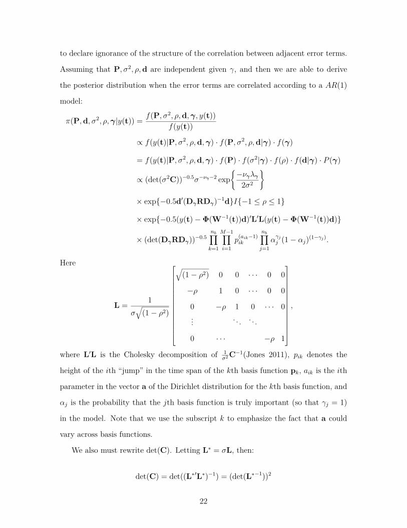
to declare ignorance of the structure of the correlation between adjacent error terms.

Assuming that P, σ2, ρ,d are independent given γ, and then we are able to derive

the posterior distribution when the error terms are correlated according to a AR(1)

model:

π(P,d, σ2, ρ,γ|y(t)) = f(P, σ2, ρ,d,γ, y(t))f(y(t))

∝ f(y(t)|P, σ2, ρ,d,γ) · f(P, σ2, ρ,d|γ) · f(γ)

= f(y(t)|P, σ2, ρ,d,γ) · f(P) · f(σ2|γ) · f(ρ) · f(d|γ) · P (γ)

∝ (det(σ2C))−0.5σ−νγ−2 exp{−νγλγ

2σ2

}

× exp{−0.5d′(DγRDγ)−1d}I{−1 ≤ ρ ≤ 1}

× exp{−0.5(y(t)−Φ(W−1(t))d)′L′L(y(t)−Φ(W−1(t))d)}

× (det(DγRDγ))−0.5nb∏k=1

M−1∏i=1

p(aik−1)ik

nb∏j=1

αγjj (1− αj)(1−γj).

Here

L = 1σ√

(1− ρ2)

√(1− ρ2) 0 0 · · · 0 0

−ρ 1 0 · · · 0 0

0 −ρ 1 0 · · · 0... . . . . . .

0 · · · −ρ 1

,

where L′L is the Cholesky decomposition of 1σ2 C−1(Jones 2011), pik denotes the

height of the ith “jump” in the time span of the kth basis function pk, aik is the ith

parameter in the vector a of the Dirichlet distribution for the kth basis function, and

αj is the probability that the jth basis function is truly important (so that γj = 1)

in the model. Note that we use the subscript k to emphasize the fact that a could

vary across basis functions.

We also must rewrite det(C). Letting L∗ = σL, then:

det(C) = det((L∗′L∗)−1) = (det(L∗−1))2

22

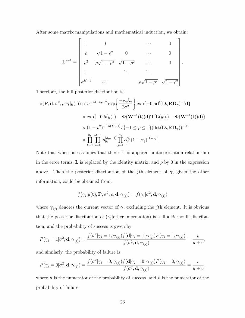
After some matrix manipulations and mathematical induction, we obtain:

L∗−1 =

1 0 · · · 0

ρ√

1− ρ2 0 · · · 0

ρ2 ρ√

1− ρ2√

1− ρ2 · · · 0... . . . . . .

ρM−1 · · · ρ√

1− ρ2√

1− ρ2

,

Therefore, the full posterior distribution is:

π(P,d, σ2, ρ,γ|y(t)) ∝ σ−M−νγ−2 exp{−νγλγ

2σ2

}exp{−0.5d′(DγRDγ)−1d}

× exp{−0.5(y(t)−Φ(W−1(t))d)′L′L(y(t)−Φ(W−1(t))d)}

× (1− ρ2)−0.5(M−1)I{−1 ≤ ρ ≤ 1}(det(DγRDγ))−0.5

×nb∏k=1

M−1∏i=1

p(aik−1)ik

nb∏j=1

αγjj (1− αj)(1−γj).

Note that when one assumes that there is no apparent autocorrelation relationship

in the error terms, L is replaced by the identity matrix, and ρ by 0 in the expression

above. Then the posterior distribution of the jth element of γ, given the other

information, could be obtained from:

f(γj|y(t),P, σ2, ρ,d,γ(j)) = f(γj|σ2,d,γ(j))

where γ(j) denotes the current vector of γ, excluding the jth element. It is obvious

that the posterior distribution of (γj|other information) is still a Bernoulli distribu-

tion, and the probability of success is given by:

P (γj = 1|σ2,d,γ(j)) =f(σ2|γj = 1,γ(j))f(d|γj = 1,γ(j))P (γj = 1,γ(j))

f(σ2,d,γ(j))= u

u+ v,

and similarly, the probability of failure is:

P (γj = 0|σ2,d,γ(j)) =f(σ2|γj = 0,γ(j))f(d|γj = 0,γ(j))P (γj = 0,γ(j))

f(σ2,d,γ(j))= v

u+ v,

where u is the numerator of the probability of success, and v is the numerator of the

probability of failure.

23

The conditional posterior distribution of (d|other parameters) is given by:

f(d|y(t), ρ, σ2,γ)

∝ exp{−0.5(y(t)−Φ(W−1(t))d)′L′L(y(t)−Φ(W−1(t))d)}

× exp{−0.5d′(DγRDγ)−1d}

∝ exp{−0.5d′{Φ(W−1(t))′L′LΦ(W−1(t)) + (DγRDγ)−1}d

− 2y(t)′L′LΦ(W−1(t))}.

It is obvious that:

d|y(t),p, σ2, ρ,γ ∼MVN(µF ,Σ),

where

µF = Σ[Φ(W−1(t))′L′Ly(t)],

and

Σ = [Φ(W−1(t))L′LΦ(W−1(t)) + (DγRDγ)−1]−1.

The posterior conditional distribution of σ2 is:

f(σ2|y(t),P, ρ,d,γ) =f(σ2|y(t), ρ,d,γ)

∝ σ−M−νγ−2 exp{− 1

2σ2

(νγλγ + (y(t)−Φ(W−1(t))d)′

× L∗′L∗(y(t)−Φ(W−1(t))d))}

.

Thus,

σ2|y(t),P, ρ,d,γ ∼ IG(α∗, β∗),

where

α∗ = M + νγ

2 ,

and

β∗ = 12

(νγλγ + (y(t)−Φ(W−1(t))d)′L∗′L∗(y(t)−Φ(W−1(t))d)

).

24

Note that the information about basis function selection is contained in the posterior

distribution of γ. We employ the posterior mode of γ as defining the most desirable

potential model, as described in George and McCulloch (1993). That is, we sample

from the joint posterior distribution in the following order: p1,p2, . . . ,pnb , σ2,d,γ,p1,

p2, . . . ,pnb , σ2, . . . . We utilize the Gibbs sampler to sample γ, σ2 and d, since their

conditional posterior distributions are known and easy to sample from, and we use

Metropolis-Hastings method within the Gibbs sampler to sample P and ρ, since their

conditional posterior distributions are not in closed form. Due to the restrictions on

each pk vector, we use a truncated normal distribution as the instrumental distribu-

tion. Let superscript (i) represents parameter values sampled at the ith iteration.

For the kth basis function, one first generates an initial p(0)k = (p(0)

1k , p(0)2k , . . . , p

(0)Mt−1k)′

from a Dirichlet prior. Then at iteration i, one samples the elements of p(i)k one by

one in the following way:

1. Sample the first element in p(i)k , p(i)

1k , by drawing a random observation from

N(p(i−1)1k , σ2

2)I(0, L1u). And then adjust the last element in p(i−1)

k , i.e., p(i−1)Mt−1k, to make

the following holds:

p(i)1k +

Mt−2∑j=2

p(i−1)jk + p

(i−1)Mt−1k = 1.

Denote the adjusted p(i−1)Mt−1k as p

∗(i)Mt−1k. Here L1

u = p(i−1)1k +p(i−1)

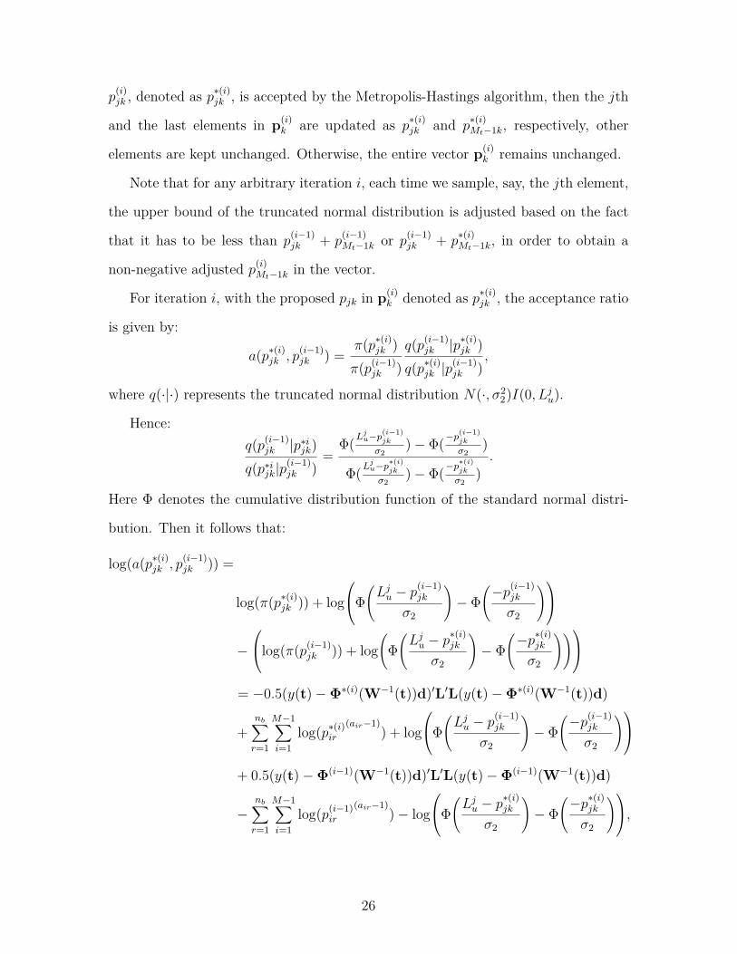
Mt−1k. If the proposed p(i)1k ,

denoted as p∗(i)1k , is accepted by the Metropolis-Hastings algorithm, then the first and

the last elements in p(i)k are updated as p∗(i)1k and p∗(i)Mt−1k, respectively, other elements

are the same as those in p(i−1). Otherwise, the entire vector p(i)k remains the same as

p(i−1)k .

2. For j = 2, 3, . . . , (Mt − 2), sample the jth element p(i)jk by drawing a random

observation from N(p(i−1)jk , σ2

2)I(0, Lju), and adjust p∗(i)Mt−1k to make the following holds:

Mt−2∑j=1

p(i)jk + p

∗(i)Mt−1k = 1.

Still denote the adjusted p∗(i)Mt−1k as p∗(i)Mt−1k. Here Lju = p

(i−1)jk +p

∗(i)Mt−1k. If the proposed

25

p(i)jk , denoted as p∗(i)jk , is accepted by the Metropolis-Hastings algorithm, then the jth

and the last elements in p(i)k are updated as p∗(i)jk and p

∗(i)Mt−1k, respectively, other

elements are kept unchanged. Otherwise, the entire vector p(i)k remains unchanged.

Note that for any arbitrary iteration i, each time we sample, say, the jth element,

the upper bound of the truncated normal distribution is adjusted based on the fact

that it has to be less than p(i−1)jk + p

(i−1)Mt−1k or p(i−1)

jk + p∗(i)Mt−1k, in order to obtain a

non-negative adjusted p(i)Mt−1k in the vector.

For iteration i, with the proposed pjk in p(i)k denoted as p∗(i)jk , the acceptance ratio

is given by:

a(p∗(i)jk , p(i−1)jk ) =

π(p∗(i)jk )π(p(i−1)

jk )q(p(i−1)

jk |p∗(i)jk )q(p∗(i)jk |p

(i−1)jk )

,

where q(·|·) represents the truncated normal distribution N(·, σ22)I(0, Lju).

Hence:q(p(i−1)

jk |p∗ijk)q(p∗ijk|p

(i−1)jk )

=Φ(L

ju−p

(i−1)jk

σ2)− Φ(−p

(i−1)jk

σ2)

Φ(Lju−p

∗(i)jk

σ2)− Φ(−p

∗(i)jk

σ2).

Here Φ denotes the cumulative distribution function of the standard normal distri-

bution. Then it follows that:

log(a(p∗(i)jk , p(i−1)jk )) =

log(π(p∗(i)jk )) + logΦ

(Lju − p

(i−1)jk

σ2

)− Φ

(−p(i−1)

jk

σ2

)−

log(π(p(i−1)jk )) + log

(Φ(Lju − p

∗(i)jk

σ2

)− Φ

(−p∗(i)jk

σ2

))= −0.5(y(t)−Φ∗(i)(W−1(t))d)′L′L(y(t)−Φ∗(i)(W−1(t))d)

+nb∑r=1

M−1∑i=1

log(p∗(i)ir

(air−1)) + log

Φ(Lju − p

(i−1)jk

σ2

)− Φ

(−p(i−1)

jk

σ2

)+ 0.5(y(t)−Φ(i−1)(W−1(t))d)′L′L(y(t)−Φ(i−1)(W−1(t))d)

−nb∑r=1

M−1∑i=1

log(p(i−1)ir

(air−1))− log

Φ(Lju − p

∗(i)jk

σ2

)− Φ

(−p∗(i)jk

σ2

),

26

where Φ∗(i)(W−1(t)) represents the adjusted “design matrix” in the ith step according

to p∗(i)jk .

2.4 Knot Selection with Reversible Jump MCMC

The flexibility of B-splines for fitting functional data is based on the knots on the time

axis. Appropriately chosen knots could result in an extremely good fit, while naively

chosen knots that do not reflect the nature of the functional curve could produce a

poorly fitted curve. Hence, we will consider both cases of fixed knots and optimally

selected knots in the simulation section.

Many methods have been developed that focus on selecting knots to improve the

performance of B-splines. We will discuss two approaches proposed by Denison et al.

(1998) and DiMatteo et al. (2001) that utilize Reversible Jump Markov Chain Monte

Carlo (RJMCMC) (Green 1995) to simulate the posterior distribution of (k, ξ), where

k denotes the number of interior knots used to connect B-splines, and ξ refers to the

locations of the k interior knots on the time axis in ascending order. RJMCMC is an

extension to the Metropolis-Hastings method that uses some proposal distribution to

propose candidate values for the parameters of interest. However it includes a “birth

jumping probability,” and a “death jumping probability” to allow for the possibility

of dimension change. It is particularly useful in cases when the “true” dimension of

the parameters is unknown and simultaneous estimation of the parameter values is

needed along with a dimension update; common settings for RJMCMC include vari-

able selection or step function estimation. The method requires having the detailed

balance property satisfied for each update to ensure the existence of a steady state

distribution. In the general scheme of both Denison et al. (1998) and DiMatteo et

al. (2001), when selecting the number and locations of the knots in functional curve

fitting, the necessary steps involved in RJMCMC are the “birth step,” “death step”

and “relocation step.” In the first two steps, the chain either accepts an increase in

27

the dimension of the parameters by having an additional proposed knot inserted into

the existing knot sequence, accepts having one of the knots deleted from the sequence,

or rejects the proposed state and stays at the current state. In the “relocation step,”

the chain determines whether to relocate one of the existing knots or not.

Because the underlying true model is not unique, we assume that with appropri-

ately chosen knots, the observed data could be adequately described with a group

of order r B-splines. The data and the “design matrix” formed by the B-splines

evaluated at those measured time points are connected via the following relationship:

y(t)|Φk,ξ(t), σ2B ∼MVNr+k(Φk,ξ(t)c, σ2

BI),

where c is the true underlying vector of coefficients corresponding to the B-splines

in the model, and σ2B is the variance of the error terms. Here the subscripts in the

notation Φk,ξ(t) are used to emphasize how both the dimension and the values of the

B-spline functions depend on the number and locations of the knots. Note that while

independent errors are assumed here, one may certainly include some autocorrelation

structure to allow for the possibility of correlated error terms. However, in a two-

stage procedure, where one first selects knots on the time axis for optimal B-splines

performance, and then uses our Bayesian model described in section 2.3 to further

improve the fit, the structure of error terms for both stages should coincide with

each other. We use the scheme given by DiMatteo et al. (2001). The prior for k is

Poisson, and ξ|k follows Dir(1,1,. . . , 1). The prior for σ2B could be chosen as inverse

gamma or the improper prior π(σ2B) ∼ 1/σ2

B. The coefficient vector has the following

conditional prior:

c|k, ξ, σ2B ∼MVN(0, σ2

BM{Φk,ξ(t)TΦk,ξ(t)}−1).

In each iteration, the three aforementioned probabilities are given by:

bk = g ·min{1, P (k + 1)/P (k)}, ek = g ·min{1, P (k − 1)/P (k)}, hk = 1− bk − ek

28

where bk is the probability of jumping from k interior knots to k + 1 interior knots.

Whether the chain at the next iteration moves to the state with an additional interior

knot depends on the acceptance ratio. Similarly, ek is the probability of jumping from

k interior knots to the state with k − 1 interior knots. Such a move may or may not

be made based on the acceptance ratio. hk is the probability of relocating one of the

existing knots.

The main discrepancy between Denison et al. (1998) and DiMatteo et al. (2001)

is that the first utilizes a not entirely Bayesian approach, but rather a quasi-Bayesian

approach to generate the chain by using least squares to calculate c values for each

proposed update of (k, ξ). According to DiMatteo et al. (2001), this would tend

to over-fit the curve to some extent. As a result, the latter proposed deriving the

distribution of c|k, ξ,Y(t) by integrating out σ2B from the joint posterior distribution

of c, σ2B|k, ξ,Y(t). Based on our investigation, it appears that even for a parametric

model, the posterior distribution of c|k, ξ,Y(t) is unlikely to be in closed form. For

the improper prior on σ2B adopted by DiMatteo et al. (2001), the corresponding

distribution is not recognizable. The aforementioned posterior distribution becomes

a multivariate non-central t distribution only when an inverse gamma prior with

equivalent shape and scale parameter values is employed for σ2B. In fact, based on our

limited simulation studies, even for irregular shaped data curves, with the maximum

number of knots set large enough, both of the aforementioned approaches are capable

of giving plausible fitting results in the sense that the mean squared error is negligible

compared with the data information. However, our primary goal is to improve the

original B-spline fit of the curves, and to compare the improved fit with the result

obtained from our method. A model with B-splines could achieve a perfect fit by

using an outrageously large number of knots, but this would produce a model too

complicated to be of any practical advantage. We want to limit the maximum number

of knots used in the procedure, and show in our simulation studies that even with

29

a limited number of knots, the performance of our approach is competitive with

using B-splines with a relatively large number of optimally selected knots. We use

least squares to estimate c in each step for computational ease and also to avoid

a distribution identifiability issue. With a limited number of knots and relatively

complicated functional data, the over-fitting concern of this quasi-Bayesian approach

noted by DiMatteo et al. (2001) would no longer be a problem.

The proposal probability for the jump from k knots to k + 1 knots is defined by:

q(k + 1|k) = bkk

k∑i=1

PB(ξ∗i |ξi).

Here ξi is the location of the ith knot, ξ∗i is the proposed new knot, which is centered

around ξi, and PB(·|·) is the proposal distribution. DiMatteo et al. (2001) claimed

that the simulation results are relatively robust to the choice of proposal distribution;

therefore, we use their proposed Beta distribution with parameters ξiν and (1 −

ξi)ν. For each existing knot, one first randomly generates a realization from the

proposal distribution that is centered at that knot. Pick at random one knot, say, ξ∗p ;

calculate the aforementioned probability; calculate the acceptance ratio; and compare

the acceptance ratio with a randomly generated uniformly distributed realization to

determine whether the proposed knot centered at ξ∗p is accepted or not.

The proposal probability for jumping from k to k − 1 knots is given by:

q(k − 1|k) = ek/k.

Similarly to the “birth step,” one randomly picks an existing knot and uses the

acceptance ratio to determine whether or not the selected knot should be deleted

from the sequence. The proposal probability for relocating one of the existing knot

is:

q(ξ∗p |ξp) = hk1kPR(ξ∗p |ξp).

We set PR(·|·) to be the same as PB(·|·). If such a move is accepted, ξp will be replaced

by the proposed ξ∗p . Therefore, in each step, the transition probabilities of moving

30

from k to k − 1 knots or from k to k + 1 knots are just the aforementioned proposal

probabilities times the corresponding acceptance ratios. See DiMatteo et al. (2001)

for detailed expression of acceptance ratios.

Note that when calculating the acceptance ratios in each step, c needs to be

updated along with the proposed (k, ξ) to match the dimensions.

2.5 Simulation Studies

In this section, we simulate some irregularly shaped functional data. We carry out

our approach and compare our approach to several alternative fitting methods: (1)

the original B-splines with fixed equally spaced knots; (2) B-splines with optimally

selected knots; (3) the Fourier basis system; and (4) the orthonormal set of wavelet

basis which include the Haar father wavelet and shifted and scaled mother wavelets.

We consider simulating a group of observations that come from a mixture of a periodic

signal, a smooth signal, and a spiky signal. In order to do that, we determine a number

of Fourier basis functions to be employed, randomly generate normal coefficients for

these, and add independent Gaussian errors to form the periodic signal. We use a

similar approach to generate a signal based on B-splines. The spiky data is generated

by first randomly partitioning the time domain into several intervals, and evaluating

the values of a baseline curve at the boundaries of those intervals. The baseline curve

is obtained from linear combinations of B-splines plus error terms. The width of each

interval represents either the width of a spike in the curve, or the spacing between a

pair of spikes. We therefore use two exponential distributions with different means

to model the spacings. The means of the exponential distributions are chosen so

that the simulated curve has a moderate number of spikes, with appropriate spacings

between them. The height of each spike is determined via the baseline value at the

center of each spike plus a randomly generated U(0, 30) observation. Then our mixed

functional data is obtained by taking a weighted average of the three curve types.

31

Some examples are described below.

Example 2.1. In this example we employ 11 Fourier basis functions and 20 order-5

B-spline basis functions with equally spaced knots to generate our simulated data.

The B-splines are measured over 500 equally spaced points in the domain [1, 5]. Their

corresponding coefficients are generated independently as Gaussian with mean 0 and

standard deviation 2. Random errors from the same distribution are added to both

curve types. The baseline curve for the spiky data is the true signal curve generated

by B-splines, plus independent N(0, 4) errors. The widths of the spikes and the

spacings between each pair of spikes are exponential with respective means 0.4 and

2/15. The weights for the three types of curves are 0.1, 0.1 and 0.8. Figure 2.3

shows the simulated noisy observed curve (solid) superimposed on the true signal

curve (dashed). We measure the signal to noise ratio by calculating the ratio of

the standard deviation of the true signal versus the standard deviation of the error

function. From investigation, it appears that roughly 2.5 to 4.5 are appropriate values

of the aforementioned ratio, so that the true signals are not overwhelmed by noise.

After standardization of the simulated data curves to scale them to exist within

the domain [0, 1], we start with order-5 B-splines, with 12 equally spaced knots on

[0, 1], and carry out our procedure to fit the data with transformed B-splines. Figure

2.4 is the trace plot of mean squared error over 1000 iterations; we see that the chain

converges rapidly after a few iterations even though the simulated curve is irregular

with several spikes. Therefore, we employ 1000 iterations for most of our settings,

since it is sufficient for us to sample from the posterior distribution. Figure 2.5 shows

a set of 15 transformed B-splines based on the 15 order-5 B-splines with a sequence of

12 equally spaced knots over [0, 1]. Each spline is twisted somewhat to accommodate

the irregular shape of the curve, yet the domains over which the transformed splines

and the original ones are positive are roughly the same. In order to obtain smooth

transformed splines while also keeping flexibility to fit irregularly shaped curves, one

32

0.0 0.2 0.4 0.6 0.8 1.0

-50

510

1520

25

t

y(t)

Figure 2.3: True versus fitted simulated curves. Dashed spiky curve: simulated true signalcurve. Solid wiggly curve: corresponding observed curve.

may want to choose the values of the elements in parameter a to be relatively small,

yet not so small that the wiggles in the splines look like step functions with sudden

jumps.

In order to smooth our fitted curve, we average the obtained curves from MCMC

iterations 200 to 1000, roughly after the area where the MSE begins to level off on

the graph. This implied a burn-in period of 200 iterations.

Figure 2.6 and 2.7 are comparison plots that superimposes several fitted curves

obtained via different methods on the true signal curve (black solid). We use “TB” to

denote our approach for functional data fitting, “B” to denote the B-splines approach

33

0 200 400 600 800 1000

26

10

iterations

MSE

Figure 2.4: Mean squared error trace plot of 1000 MCMC iterations

0 100 200 300 400 500

0.0

0.2

0.4

0.6

0.8

1.0

t

splin

e va

lue

Figure 2.5: Example of set of 15 transformed B-splines obtained from one MCMC iteration

with equally spaced knots, “SKB” to denote the B-splines approach with knots se-

lected via RJMCMC, and “Wave” and “Fourier” represent fitting via the wavelet

basis or the Fourier basis. Here we are using 16 instead of 15 wavelet basis functions,

since the number of wavelet basis functions employed in a fitting procedure must be

2res, where res is the resolution value. “STB” denotes our approach with reduced

dimension. More specifically, to obtain the STB fit for the observed curves, we do the

following: For each iteration, we obtain a sequence of basis functions selected along

with other parameter values. We then calculate the frequencies of different sequences

34

0.0 0.2 0.4 0.6 0.8 1.0

05

1015

20

t

y(t)

TruthTBBSKB

Figure 2.6: True signal curve versus fitted curves from three competing methods. Blacksolid curve: true signal curve. Red dashed curve: fitted curve obtained from Bayesiantransformed B-splines method. Blue dotted curve: fitted curve obtained from B-splinesbasis functions. Dashed green curve: fitted curve obtained from B-splines basis functionswith selected knots.

of basis functions being selected. Usually there is one or two sets of basis functions

that are selected with overwhelming frequency. These are the potential sets of basis

functions to be included in the model. Next we select the iterations in the chain that

have the same set of basis functions appearing most frequently. Following that, we

obtain least squares estimates for the coefficients of the basis for each iteration in

the subset, and hence obtain estimates for the original curves. Finally we average

those fitted curves and take that as our STB fit. Note that even though the basis

function shapes change from iteration to iteration, after a certain point (i.e., after

the MSE values level off), such change is negligible and only represents randomness

35

0 100 200 300 400 500

05

1015

20

t

y(t)

TruthTBWaveFourier

Figure 2.7: True signal curve versus fitted curves from three competing methods. Blacksolid curve: true signal curve. Red dashed curve: fitted curve obtained from Bayesiantransformed B-splines method. Blue dotted curve: fitted curve obtained from the waveletbasis functions. Dashed green curve: fitted curve obtained from the Fourier basis functions.

of the Markov chain. Similarly, the SKB fit is obtained by first checking the MSE

plot to determine the number of iterations i after which the MSE values become sta-

bilized, obtaining the number of knots ksel that appear with the greatest frequency

in the chain, then selecting all iterations with ksel knots selected, and averaging the

estimated curves from the set of chosen iterations after the ith. Again, even with the

same number of knots selected, the locations of the knots vary for different iterations

in the set. Yet still, the estimated curves stabilize after the ith iteration, as the

MSE values stabilize. We set the maximum possible number of knots, kmax, to be

12 in this setting, making the greatest possible dimension of the B-spline model 15.

In practice, for these irregular simulated data, the RJMCMC procedure for knot

36

Table 2.1: MSE comparison table for five smoothing methods. Top: MSE values calculatedwith respect to the observed curve. Bottom: MSE values calculated with respect to thetrue signal curve.

TB STB B SKB Wave FourierObs 0.88 3.61 13.06 9.10 13.05 12.43Truth 0.86 2.84 11.70 8.15 12.17 11.05

selection always leads to the maximum number of knots appearing with the greatest

frequency, making the dimension of the SKB model exactly 15. SKB does a better

job than B in capturing the peaks and troughs of the curves, yet with its limited

dimension, it cannot achieve a desirable fit, either. Among the several fitted curves

in the comparison plots, ours (red) performs the best. Table 2.1 compares the MSE

values (with respect to the true signal curve and to the observed curve) obtained via

the aforementioned fitting approaches.

Example 2.2. Using the same simulation setting, with different weightings of the

three curve types, we now compare the performances of different fitting methods.

Table 2.2 summarizes the MSE values resulting from the comparative approaches.

The three numbers in the first cell of each row represent the weighting of re-

spectively: the periodic curve generated from the Fourier basis, the smooth curve

generated from B-splines and the spiky curve obtained from the method described

previously. The number in each upper sub-cell in the interior of the table is the

MSE of the fitted curve obtained via the corresponding method with respect to the

observed curve, and the value in the bottom sub-cell is the MSE with respect to

the true signal curve. For different weightings, the error terms added for each curve

type might be different, in order to maintain the signal-to-noise ratio. The value in

bold in each row is the row minimum, and the value in italics is the second smallest

MSE value in the row. Our approach almost always achieves a much smaller MSE

compared with other fitting methods.

37

Table 2.2: MSE comparison table for six smoothing methods. Digits in the Weightscolumn represent the weighting of the simulated periodic curve, smooth curve and spikycurve, respectively. Top row in each cell: MSE value calculated with respect to the observedcurve. Bottom row in each cell: MSE value calculated with respect to the true signal curve.

Weights B SKB Wave Fourier TB STB100 2.621 2.415 6.385 2.562 1.800 1.805

0.325 0.323 3.895 0.268 0.372 0.448010 0.216 0.173 0.381 0.224 0.158 0.153

0.039 0.023 0.189 0.082 0.018 0.019001 20.880 6.252 22.818 26.151 2.470 3.904

18.507 4.682 20.860 23.720 1.669 3.38513

13

13 2.250 1.263 2.150 1.749 0.439 0.465

1.770 0.754 1.730 1.237 0.180 0.19912 0 1

2 6.416 3.444 6.558 7.567 1.185 1.7575.437 2.515 5.375 6.442 0.700 1.355

0 12

12 2.424 2.160 3.890 3.747 0.563 0.609

3.188 1.502 3.307 3.046 0.253 0.29512

12 0 0.295 0.223 0.991 0.315 0.191 0.192

0.069 0.032 0.800 0.099 0.030 0.02912

14

14 0.907 0.504 1.821 0.912 0.108 0.114

0.773 0.378 1.650 0.708 0.075 0.07714

14

12 4.738 3.767 5.890 5.077 0.760 1.299

3.552 2.419 4.450 3.571 0.360 0.89614

12

14 1.023 0.662 1.091 0.768 0.303 0.306

0.707 0.418 0.792 0.509 0.154 0.164

2.6 Real Data Application

In this section we include some results for fitting an ocean wind data set taken from

the National Oceanic and Atmospheric Administration (NOAA). This data set is

analyzed in Hitchcock, Booth and Casella (2007) for exploring the effects of data

smoothing on data clustering. The entire data set is accessible via the historical

data page of National Buoy Data Center: http://www.ndbc.noaa.gov/hmd.shtml

(Hitchcock et al. 2007). At each of four regional locations (Northeast, Southeast,

Eastern Gulf and Western Gulf), average hourly wind speeds are collected. The

data observations could be viewed as functional data since wind speed is intrinsically

continuous and that each data point is calculated based on a continuous measure of

wind speed during hourly periods. For our analysis, we fit the same subset of 18

38

0 50 100 150

05

1015

t

y(t)

0 50 100 150

05

1015

t

y(t)

Figure 2.8: Observed versus smoothed wind speed curves. Top: four observed windspeed curves. Bottom: four corresponding wind speed curves smoothed with Bayesiantransformed B-splines basis functions.

curves analyzed in Hitchcock et al. (2007), where only the measurements from the

first 7 days of 2005 are used.

The first graph in Figure 2.8 shows four observed sample wind speed curves. The

original patterns of the curves are somewhat masked by measurement error. The

second graph in Figure 2.8 exhibits four corresponding fitted curves obtained via our

approach. Each pair of observed and smoothed curves are draw with the same color.

Figure 2.9 shows side-by-side boxplots of MSE values for fitted curves, corresponding

to 18 functional ocean wind speed observations, obtained via different methods (i.e.,

39

SKB B Wave Fourier TB

01

23

45

Figure 2.9: Side by side boxplots of MSE values for five smoothing methods. From left toright: boxplot of MSE values for 18 ocean wind curves smoothed with the selected knotsB-splines (SKB); the B-splines with equally selected knots (B); the Wavelet basis (Wave);the Fourier basis (Fourier) and the Bayesian transformed B-splines (TB).

B, SKB, Wave, Fourier, TB).

For this data set, we start with order-6 B-splines with 8 knots to carry out our

analysis. Note that one should only choose an odd number of Fourier basis functions

so that the same number of sine and cosine terms are used when fitting functional

data; thus we use 13 Fourier basis functions. Since the wavelet basis requires the

number of knots to be a power of 2, we use 16 basis functions. For the SKB method,

for each of the 18 observations, theRJMCMC procedure inevitably chose the number

of knots to be kmax (i.e., 8) most frequently, due to the several oscillations and

spikes in the curves, and the small value of kmax. Therefore, for all the observations

analyzed, the SKB method in fact used 12 basis functions for data fitting. Thus the

comparison for MSE is relatively unprejudiced in terms of model dimension, except

that the wavelet basis and the Fourier basis have slightly higher dimensions. The

40

boxplots show that our method has an obvious advantage, in terms of MSE values,

in fitting the wind data set.

2.7 Discussion

We have proposed a Bayesian approach for functional data fitting via basis systems.

Our method surpasses the shape-dependent limitations of currently popular basis

systems, e.g., polynomial splines, B-Splines, Fourier Bases, wavelet bases, in func-

tional data fitting. It adapts splines flexibly in accordance with a variety of shapes of

curves. Using a data-dependent transformation of individual splines, fit accuracy is

improved compared to existing basis systems, with model dimension remaining small

to moderate.

In our approach, time distortion is no longer applied to the entire observation to

align data, but rather on each individual spline function. The application of the time

warping function to the splines allows the domain of the transformed splines to be

roughly the same as the original splines, making the design matrix band-structured for

computational efficiency. In fact, as long as the time grid on which transformation is

applied is sufficiently fine relative to the measured time sequence, the posterior splines

remain smooth, and shifts on the domains of the splines, if any, are negligible. In

this article, our approach is based on B-splines, i.e., we impose time transformations

on individual B-splines to obtain posterior splines, and we compare the fitting results

with the optimal performance of B-splines. Certainly the method is not restricted

to B-splines as the starting basis functions; one may also consider other possible

transformation options.

The combination of time transformation on individual basis functions and Bayesian

modeling is a novel approach to functional data fitting. It achieves similar goals as

employing multiple resolution basis systems and carrying out a basis selection, yet

avoids the heavy computational workload.

41

Chapter 3

Functional regression and clustering with

functional data smoothing

Summary: This chapter includes some investigation of functional data regression and

clustering, in order to evaluate the effects of our fitting method introduced in chapter

2 in functional data-related applications.

3.1 Introduction

Functional Regression

As with individual random variables whose variability can be analyzed by studying

their relationships with other variables, functional data lend themselves to similar

methods like regression or ANOVA in a functional setting. Usually, linear models

involve functional variables in one of the following three ways: either the response

variable is functional and the predictor(s) scalar, or some or all of the predictors are

functions and the response is scalar, or both the response and one or more of the

predictor variables are functions. The main difference between regression or ANOVA

in the functional setting and in the traditional sense is that the intercept term and

all the coefficients relating to functional predictors are also functions. Typically, how

the functional regression model is built must depend on one’s insight about how the

response variable is related to the predictors, whether functional or scalar.

The concurrent model is frequently employed when both the response variable

and some of the predictor variables are functional, and when one believes that the

42

response variable value measured at any point t in the time interval T is only related

to the value at the equivalent time within the functional predictor. The concurrent

model at time t with only one functional predictor is as follows:

y(t) = α(t) + x(t)β(t) + ε(t)

Here the response variable is measured at a fine grid of time points in T . β(t)

quantifies the impact of predictor x at time t on the value of y(t). By carrying out

pointwise regression at each time point t, we get estimates of α(t) and β(t). And

combining α(t) and β(t) for all the measured time points t in t, we obtain estimated

curves for the true intercept function α(·), and for the coefficient function β(·).

When one believes that the response variable is related to the derivative of one

or more predictors, or there are some interactions between the predictors, or between

the derivative of some predictor and some other predictors, the interaction model or

derivative model is implemented.

There are many other models in the realm of functional regression, but we will

be mostly focusing on the models discussed above as our simulations and real data

examples suit the aforementioned model well.

Functional Clustering

Another mostly used application in the realm of functional analysis is functional clus-

tering. Functional clustering methods are very similar to traditional cluster analysis

methods. One starts by calculating distances between all pairs of curves to be clus-

tered to form a distance matrix. One most commonly used distance measure is the

Euclidean distance, or the L2 norm:

dL2 [yi(t), yj(t)] =√∫

[yi(t)− yj(t)]2dt = dij

Popular functional clustering methods can be directly applied to the distance matrix

obtained from the original set of curves.

43

Currently, popular clustering methods include but are not limited to hierarchical

based methods with different types of linkages, partitioning methods such as the

K-means and the K-medoids methods, and a hybrid method, Ward’s method.

The hierarchical methods typically start with each observation being a individual

cluster, and joining the two closest clusters in each step. Here, the closeness between

two clusters is measured differently depending on the linkage employed. The single

linkage method joins the two clusters C1 and C2 with the smallest distance ds as

measured by:

ds = mini∈C1,j∈C2

(dij).

Since it only depends on the minimal distance between any pair of curves, the single

linkage based hierarchical clustering results can be unreliable. As opposed to single

linkage, complete linkage is based on the maximal distance dc for all pair of curves,

which is given by:

dc = maxi∈C1,j∈C2

(dij).

The complete linkage is better than single linkage, since it depends on the farthest

distances for all pairs of curves. Another linkage option is called the average linkage,

which joins the two clusters based on the minimal of the following distance da:

da = 1n1n2

∑i∈C1

∑j∈C2

(dij).

Here n1 and n2 are the total number of items in clusters C1 and C2, respectively. This

linkage utilizes the most information possible from all the observations to determine

distance between clusters.

Another category of clustering methods is the partitioning methods, and the most

popular clustering methods in this category include K-means and K-medoids cluster-

ing. Unlike hierarchical methods, which form tree type results as part of the clustering

procedure, the partitioning methods typically try to search for an optimal partition of

the original observations into K clusters by minimization of some “summed distance

44

measure”. Such methods start from randomly partitioned K clusters, or K “centers”,

called centroids, and repeatedly switch the clustering membership for each item in

the pool until no new partition could result in a smaller summed distance measure

defined for the corresponding approach.

Ward’s clustering method, on the other hand, falls in a third category, which

is in fact a hybrid of the hierarchical method and the partitioning method, in the

sense that it starts from each observation being its own cluster, and joins the two

clusters that will lead to the smallest “summed distance measure” at each step, until

all observations are joined into one big cluster. Tree cutting techniques can be used

to obtain clusters of desirable size.

The fitting method we proposed in Chapter 2 provides an alternative to commonly

used smoothing methods such as the B-splines, the Fourier basis, the wavelet basis,

etc. We are specifically interested in the applications of our fitting method, to see

whether it leads to improvements in statistical analyses and how such improvements

compete with those resulting from employing other fitting methods before carrying

out functional data applications. Our investigation focused on functional regression

and functional clustering. In sections 3.2 and 3.3, we discuss simulated data examples

for functional clustering and functional regression, respectively. And in sections 3.4

and 3.5, we give two real data functional regression examples.

3.2 Simulation Studies: Functional Clustering

This section includes some investigation of the influence of our functional data

smoothing method on functional data clustering, to see whether our method gives

competitive results in terms of accurately clustering the curves. We have simulated

a total of four clusters of 23 curves, each of length 200, where three of the clusters

each have 6 curves, and one cluster has 5. Figure 3.1 shows the 23 raw data curves,

where curves coming from the same cluster are plotted with the same color and line

45

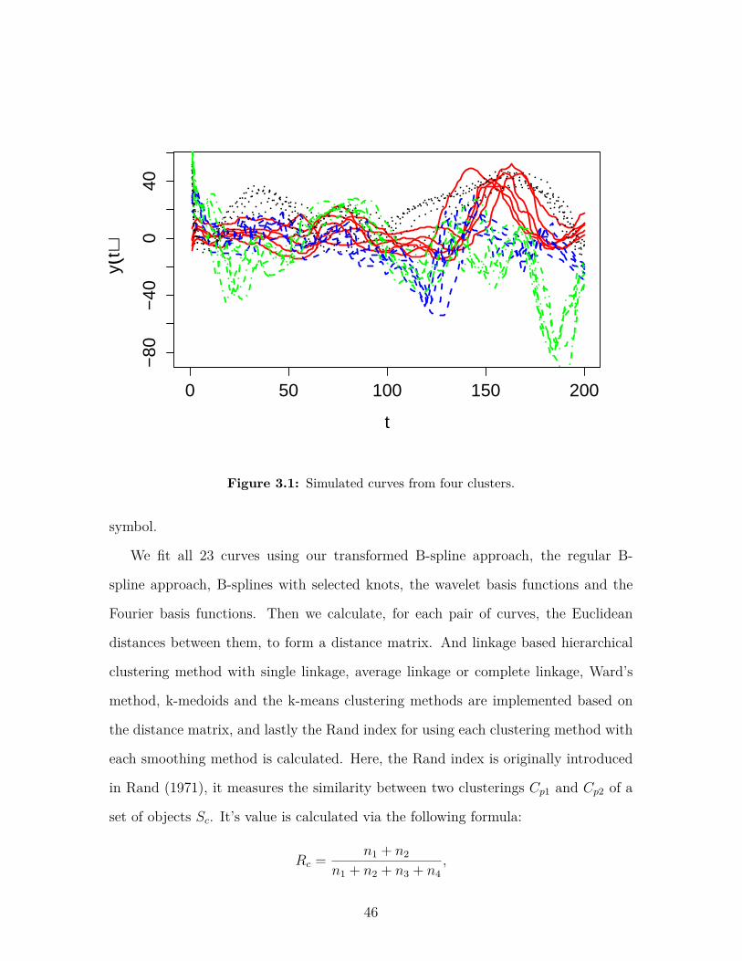
0 50 100 150 200

−80

−40

040

t

y(t)

Figure 3.1: Simulated curves from four clusters.

symbol.

We fit all 23 curves using our transformed B-spline approach, the regular B-

spline approach, B-splines with selected knots, the wavelet basis functions and the

Fourier basis functions. Then we calculate, for each pair of curves, the Euclidean

distances between them, to form a distance matrix. And linkage based hierarchical

clustering method with single linkage, average linkage or complete linkage, Ward’s

method, k-medoids and the k-means clustering methods are implemented based on

the distance matrix, and lastly the Rand index for using each clustering method with

each smoothing method is calculated. Here, the Rand index is originally introduced

in Rand (1971), it measures the similarity between two clusterings Cp1 and Cp2 of a

set of objects Sc. It’s value is calculated via the following formula:

Rc = n1 + n2

n1 + n2 + n3 + n4,

46

Table 3.1: Rand index values for five smoothing methods based on regular distance matrix

TB B SKB Fourier Wavesingle 0.826 0.862 0.613 0.672 0.862average 1 1 1 1 1complete 1 1 1 1 1ward 1 1 1 0.957 0.921

k-medoids 1 1 1 1 1k-means 0.957 0.957 0.957 0.957 0.957

Table 3.2: Rand index values for five smoothing methods based on standardized distancematrix

TB B SKB Fourier Wavesingle 0.632 0.625 0.625 0.632 0.842average 0.957 0.957 0.957 0.838 0.957complete 0.957 0.814 0.957 0.802 0.957ward 0.957 0.957 0.957 0.866 0.957

k-medoids 1 0.957 1 0.960 1k-means 1 0.822 0.866 1 0.957

where n1, n2, n3 and n4 are the numbers of pairs of objects from the sample Sc that

are: assigned to the same cluster in Cp1 and the same cluster in Cp2, assigned to

different clusters in Cp1 and different clusters in Cp2, assigned to the same cluster

in Cp1 but different clusters in Cp2 and assigned to different clusters in Cp1 but the

same cluster in Cp2, respectively. Hence, Rand index values close to 1 implies great

similarity of the two clusterings Cp1 and Cp2 of the curves, otherwise, Rand index

values close to 0 suggests great discrepancies between Cp1 and Cp2.

Table 3.1 gives the Rand index values based on the regular distance matrix, with

each of the aforementioned smoothing methods applied to the data prior to data

clustering. And Table 3.2 gives the Rand index values based on the standardized

distance matrix, in which each measured point in each curve has the mean value for

all 23 curves measured at the same time point subtracted from it, and is divided by

its standard deviation across the 23 curves. For both tables, except for the hierarchi-

47

cal clustering method with single linkage (in which case the wavelet basis smoothing

seems to give the best clustering accuracy) for all other clustering methods imple-

mented, our transformed B-spline basis smoothing produces clusters whose accuracy

is no worse than all other competing methods. Hence, from the functional clustering

perspective, our smoothing method does produce competitive results as measured by

Rand index.

3.3 Simulation Studies: Functional Regression

We are specifically interested in exploring whether smoothing functional data prior

to functional regression will lead to improvement in parameter estimation and pre-

diction accuracy, and if so, which of the currently popular methods would lead to

comparatively greater improvement. This may depend on what criterion we use to

judge what “better” means.

In this study, the smoothing methods under comparison are the same as those

used in Chapter 2, i.e., a B-splines fitting method with equally spaced knots, a B-

spline basis with optimally chosen knots, the Fourier basis, the wavelet basis, and our

Bayesian approach. Intuitively, we may conjecture that not applying pre-smoothing

techniques on functional data prior to carrying out regression analysis, i.e., the naive

approach, would lead to the worst regression prediction and estimation, since error

terms in the data may mask the true signal, and good smoothing methods tend to

separate error from data. However, based on our simulation investigations, the results

do not necessarily match those intuitive expectations.

In the following simulation studies, we focus on the one predictor scenario, in

which both the response and the predictor variables are functions of the same time

interval T . Our true predictor variable signal is simulated to be a linear combination

of periodic parts, a smooth part and a spiky part. The periodic part consists of several

sine and cosine functions, the smooth part is simply a polynomial function, and the

48

spiky part is generated via a random Poisson realization to determine the number

of spikes in each curve, exponential realizations to determine the heights of those

spikes in each curve, and uniform realizations to determine the width of each spike.

The intercept α(·) and coefficient function β(·) are specified as smooth functions. We

generated 16 response and predictor curves using the same α(·) and β(·). Since for

regression analysis, the spread of the values of the predictor influences the accuracy of

estimation, we adjusted the ranges for the predictor curves to be somewhat different,

by adding constant shifts to the original generated predictor curves if necessary.

Assuming that both the response and the predictor are observed over a relatively

fine grid of time points in T , realizations of the Ornstein-Uhlenbeck process are ap-

plied to generate the discretized error vectors, which are added to the signal response

and predictor vectors to obtain the observed vectors. The Ornstein-Uhlenbeck (O-U)

process is a stochastic process that used to model a continuous random noise process.

The O-U process is realized via the following differential equations:

dXt = −θXtdt+ dWt,

with X0 = x0, and Wt is the Wiener process. For the O-U process, both the time t

and the distances δt between Xt and Xt+δt play a role in determining the structure

between them. After the data are generated, the smoothing methods mentioned

above are applied on both the response and predictor discretized functions.

For each measured time point t, we carry out a pointwise functional regres-

sion analysis, where we concatenate the response values (either smoothed or non-

smoothed) of all 16 response curves evaluated at t to form the response vector, and

do the same for the predictor curves (either smoothed or non-smoothed) to obtain a

vector of predictor values evaluated at t. Then we use OLS to obtain the fitted values

of α(t) and β(t). After carrying out the pointwise regression for all t, by concatenat-

ing the estimated α(t) and β(t) for all t values, we obtain the entire estimated α and

49

Table 3.3: In-sample SSE comparison for functional regression predictions based on sim-ulated curves

NS TB Fourier Wave BTruth 445621.7 298331 1696082.2 2356412.1 832983.6Obs 503622.3 447916.5 1809552.5 2508167.1 977643.3

β functions. Model fit is assessed by:

SSE =∑i

∑t

(y∗i (t)− α(t)− xi(t)β(t))2,

where y∗i (t) is the ith true signal response, xi(t) is the smoothed predictor evaluated

at point t, β(t) is the estimated coefficient curve and α(t) is the estimated inter-

cept curve, where some smoothing method is applied to α(t) to correct for apparent

roughness.

In our comparison, we fix the number of basis functions across different smooth-

ing methods under comparison. It turns out that naive regression (i.e., with no

presmoothing on the curves) does well in estimating β, and the SSE value is even

smaller than most competing methods that apply pre-smoothing on the data (as will

be shown in Table 3.3). The reason could be that the number of basis functions em-

ployed for different smoothing methods is relatively small and is insufficient to capture

the structure of the simulated data; therefore, they tend to underfit the curves. On

the other hand, a closer look at the naive regression reveals that it tends to overfit

the data, and thus may do poorly if one extrapolates the measured time points into

an out-of-sample set of points t∗ in T .

The results comparing the “SSE” values defined above for the predicted response

curves with respect to either the true signal curves or the observed response curves,

without smoothing versus with presmoothing on both the response and the predictor

variables via different smoothing methods are shown in Table 3.3. Here, “NS” denotes

no smoothing on either the response or the functional predictor. Other notations are

50

the same as in Chapter 2.

We can see that the SSE values with respect to the observed curve and the true

curve are both smallest if the response and the predictor curves are fitted using our

method. Note that the SSE values are on a very large scale. This is because the

values are calculated as the sum of SSE’s for 16 curves accumulated over a total

of 100 time points. The SSE values for the individual fitted curves are shown in

Figure 3.2. This graph includes 9 boxplots of SSE values for 9 predicted response

curves with respect to the true signal curves, with presmoothing of the curves based

on the five competing methods shown in Table 3.3. The red reference line on each

boxplot gives the SSE value of the predicted response curves with our presmoothing

approach. Apparently, for the majority of the cases, using our smoothing method

prior to carrying out the functional regression model produces the predicted response

curves with relatively small SSE values, compared to other competing methods such

as “NS” (no smoothing), “Fourier”, “Wave” and “B”.

Figures 3.3 and 3.4 give 9 true signal response curves versus predicted response

curves in scenarios when the response and predictor curves are used directly in func-

tional regression, or when they are presmoothed using “TB”, “Fourier”, “Wave” or

“B”. On each individual plot of Figure 3.3, the black spiky curve represents the true

signal response curve, the purple wiggly curve represents the predicted response with

no presmoothing of the curves, the red and green dashed curves represent the scenario

when the response and the predicted curves are presmoothed using the transformed

B-splines method or the Fourier basis functions, respectively. On each individual plot

of Figure 3.4, the black spiky curve and red dashed curve are the same from those

in Figure 3.3, and the green and blue dashed curves represent the predicted response

with presmoothing using the B-spline or the Wavelet basis functions, respectively. In

all of these individual plots, it is shown that our approach in Chapter 2 tends to give

the best predictions in the sense that those predicted curves not only are smooth in

51

50000

200000

SSE

40000

120000

SSE

50000150000

SSE

20000

35000

SSE

5000

25000

SSE

50000

250000

SSE

0e+00

3e+05

SSE

0100000

SSE

5000

20000

SSE

Figure 3.2: Boxplots of SSE values for the first 9 predicted response curves with no pres-moothing or presmoothing using the transformed B-splines, the Fourier basis, the Waveletbasis and regular B-splines basis functions on the curves. Red line: SSE value for the pre-dicted response curves with presmoothing on the curves using the transformed B-splines.

nature, but they are capable of capturing the spikes on the curves that other compet-

ing methods tend to miss. The method employing the unsmoothed curves tends to

overfit, although it has smaller SSE than the Fourier smoother, which tends to miss

the peaks.

We also check out-of-sample prediction SSE for the five different methods. We

52

0 20 40 60 80 100

0100

300

t

y(t)

0 20 40 60 80 100-200

0200

t

y(t)

0 20 40 60 80 100

-300

-100

100

t

y(t)

0 20 40 60 80 100

-100

050

t

y(t)

0 20 40 60 80 100

-150

-50

050

t

y(t)

0 20 40 60 80 100-200

200

600

t

y(t)

0 20 40 60 80 100

-600

0400

t

y(t)

0 20 40 60 80 100

-200

0200

t

y(t)

0 20 40 60 80 100

-100

-50

050

t

y(t)

Figure 3.3: The first 9 predicted response curves. Black spiky curves: true signal responsecurves. Red long dashed curves: predicted curves with presmoothing using the transformedB-splines. Purple wiggly curves: predicted response curves with no presmoothing on thecurves. Green dashed curve: predicted response curves with presmoothing using the Fourierbasis functions.

53

0 20 40 60 80 100

0100

300

t

y(t)

0 20 40 60 80 100-200

0200

t

y(t)

0 20 40 60 80 100

-200

0200

t

y(t)

0 20 40 60 80 100

-50

050

t

y(t)

0 20 40 60 80 100

-100

-50

050

t

y(t)

0 20 40 60 80 100-200

200

600

t

y(t)

0 20 40 60 80 100

-600

0400

t

y(t)

0 20 40 60 80 100

-200

0200

t

y(t)

0 20 40 60 80 100

-60

-20

20

t

y(t)

Figure 3.4: The first 9 predicted response curves. Black spiky curves: true signal responsecurves. Red long dashed curves: predicted curves with presmoothing using the transformedB-splines. Blue wiggly curves: predicted response curves with with presmoothing using theWavelet basis functions. Green dashed curve: predicted response curves with presmoothingusing the regular B-spline basis functions.

54

Table 3.4: Out-of-sample SSE comparison for functional regression predictions based onsimulated curves

NS TB Fourier Wave BTruth 221460 171169.2 871350.5 851409.2 538283.3

have generated a random sample of 100 time points across [0, 1], and have our true

and predicted response curves extrapolated to those time points, and calculated the

SSE values as defined earlier for the aforementioned set of competing methods. See

Table 3.4. Again our method gives the smallest SSE as compared with others.

Note that similarly to Chapter 2, we are utilizing roughly the same number of

basis functions for the different smoothing procedures prior to functional regression.

In fact, one may get nearly perfect fit of functional data via most fitting methods

such as the wavelet basis, as long as one allows a sufficiently large number of basis

functions to be employed. However, in practice, one does not want a model that

utilizes a number of basis functions that is too large, due to computational speed

and model parsimony concerns. That is the reason that we are restrict all compet-

ing methods to employ the same number of basis functions for comparison purposes.

For some other currently popular B-splines related methods, such as the traditional

B-spline basis or the selected knots B-spline basis methods, smooth and accurate fits

could only be obtained as long as one chooses the order of the basis functions, the

number and locations of the knots wisely. However, knot selection remains a difficult

problem even today. In most cases the “optimal” knots selected in practice are not

truly optimal. Hence one common problem of these fitting methods is that when

given functional curves that are complicated in structure, especially those that are

locally highly irregular in some regions while smooth in other areas, it is hard to

determine the appropriate number of basis functions to use to obtain a desirable fit.

One may choose a relatively large number of basis functions, hoping to achieve an

55

accurate fit, yet a an accurate fit in local irregular areas may lead to over-fitting in

other smooth areas. On the other hand, if one chooses a small to moderate number

of basis functions to begin with, the true curve may be poorly fitted. However, our

approach does not encounter problems like these. A balance between accuracy and

smoothness can always be achieved even without tools like the roughness penalty

term. Relative accuracy is achieved due to the flexibility attained brought by adding

time distortion to each of the basis functions, even if one starts with few basis func-

tions, and smoothness is obtained by taking the average of the fitted curves from these

stabilized MCMC iterations once convergence is attained, since the randomness in

the time-warping from iteration to iteration is smoothed out by this simple step. This

is one vital difference between traditional fitting methods and our approach, i.e., the

basis functions contain subtle changes from iteration to iteration, and convergence of

their individual shapes is achieved when the number of iterations is large enough.

In this simulation studies, we have smoothed the estimated α(t) functions obtained

via different smoothing methods using a moderate number of B-spline basis functions,

since they were all oscillating and lacked smoothness. The estimated α(t) functions

seem to play the role of an offset since the β(t) functions are all relatively smooth.

This step is not necessarily vital, due to the fact that the α(t)’s have relatively small

range compared with that of the simulated curves themselves.

In sum, this simulation study gives us evidence of improvement in prediction

accuracy in functional regression, when our approach is utilized to presmooth the

curves, and such improvement is competitive with many other currently popular

smoothing methods. However, one may be aware that more accurate fitting of the

curves are not always linked with better prediction accuracies. In fact, in some

examples shown later, at times consistently underfitting or overfitting the curves may

lead to good prediction accuracy as well. Hence, if the goal is solely to study the

patterns of the true underlying functional form of the curves, then our approach is

56

a wise choice. But when the objective is performing functional applications such as

functional regression or clustering, then our method serves as an alternative fitting

approach in the realm of functional data fitting methods, which are expected to

improve the statistical inference results to some extent. But depending on the specific

situation, there still might be circumstances when, surprisingly, no smoothing or some

other smoothing methods (even though they may not give smooth and accurate fits

of the curves) may lead to the best performance; hence one must not make sweeping

conclusions.

3.4 Real Data Application: Functional Regression Example 1

In the following two sections, we explore the performance and potential of our func-

tional data smoothing method on real functional regression applications. Our data

comes from the website http://www.wunderground.com/history/, where the historical

weather data on any given city can be found. We take one year of weather data for

Orlando, FL. In our data set, there are daily temperature, dew point, humidity, sea

level pressure, visibility, etc. We carry out a functional regression using this data set.

We employ daily temperature as the response variable, and since temperature is intu-

itively mostly related to dew point and(or) humidity, we include both dew point and

humidity in the model, and we explore the effect of our and other fitting methods on

the predictions of multiple functional regression. We denote the temperature function

as T (·), dew point as D(·), and humidity as H(·). Our one year data set is split into

four 3-month sections, and each of the 3-month daily temperature function serves

as a response curve. Hence we have four pairs of 3-month dew point and humidity

functions as predictor curves, accordingly. To test whether our smoothing method

leads to improvement on this real data set, we smooth all of the raw response and

predictor curves, and for each method, we fit three competing models:

T (t) = α1(t) +D(t)β11(t) +H(t)β12(t) + ε(t),

57

Table 3.5: SSE comparison table: Model 1: both dew point and humidity are predictors.Top: SSE for predicted response curves with respect to the true observed curve, no furthersmoothing on α1(t), β11(t) and β12(t). Bottom: SSE for predicted response curves withrespect to the true signal curve, with further smoothing on α1(t), β11(t) and β12(t) usingregular B-spline basis functions.

NS TB Fourier Wave BSmoothed 10851.7 5426.0 7273.0 25843.0 6953.7

Unsmoothed 6267.6 4280.1 7216.2 25883.0 6964.1

Table 3.6: In-sample SSE comparison: Model 2: dew point is the only predictor. Top: SSEfor predicted response curves with respect to the true signal curve, no further smoothingon α2(t) and β1(t). Bottom: SSE for predicted response curves with respect to the trueobserved curve, with further smoothing on α2(t) and β1(t) using regular B-splines basisfunctions.

NS TB Fourier Wave BSmoothed 25697.8 21421.8 22899.3 42294.8 21375.0

Unsmoothed 17771.0 17751.5 20898.6 38577.0 20397.6

T (t) = α2(t) +D(t)β1(t) + ε(t),

T (t) = α3(t) +H(t)β2(t) + ε(t).

Each of these three models is fitted after five competing smoothing methods are

performed on the raw response and predictor curves, i.e., “NS”, “TB”, “B”, “Wave”

and “Fourier” as defined earlier. Once the coefficient curves are obtained, they are

either further smoothed using regular B-spline basis functions with a sequence of

equally spaced knots (order 10 basis functions with 15 knots located evenly across (0,

1)), or left unsmoothed, and the estimated coefficient functions are used to produce

predictions for all 4 response curves. Lastly, SSE values for all the predicted curves are

calculated for each competing smoothing method, with or without further smoothing

on the estimated coefficient curves.

The SSE values are given in Tables 3.5, 3.6 and 3.7. For all three models, our

method tends to give the smallest SSE, or better predictions for the response curves.

58

0 20 40 60 80

4050

6070

80

t

y(t)

0 20 40 60 80

5560

6570

7580

85t

y(t)

0 20 40 60 80

6570

7580

8590

t

y(t)

0 20 40 60 80

6065

7075

8085

90

t

y(t)

Figure 3.5: True Orlando temperature curves and predicted response curves withoutdata smoothing, or with data presmoothed using the transformed B-spline basis and theFourier basis functions. Black solid curve: true Orlando weather curves. Green solid curve:predicted curves without any data smoothing. Red solid curve: predicted curves withdata presmoothed using the transformed B-spline basis functions. Purple dashed curve:predicted curves with data presmoothed using the Fourier basis functions.

59

0 20 40 60 80

4050

6070

80

t

y(t)

0 20 40 60 80

5560

6570

7580

85t

y(t)

0 20 40 60 80

6570

7580

8590

t

y(t)

0 20 40 60 80

6065

7075

8085

90

t

y(t)

Figure 3.6: True Orlando temperature curves and predicted response curves with datapresmoothed using the transformed B-spline basis, regular B-spline basis functions andthe wavelet basis functions. Black solid curve: true Orlando weather curves. Green solidcurve: predicted curves presmoothed using the wavelet basis functions. Red solid curve:predicted curves with data presmoothed using the transformed B-spline basis functions.Purple dashed curve: predicted curves with data presmoothed using regular B-spline basisfunctions.

60

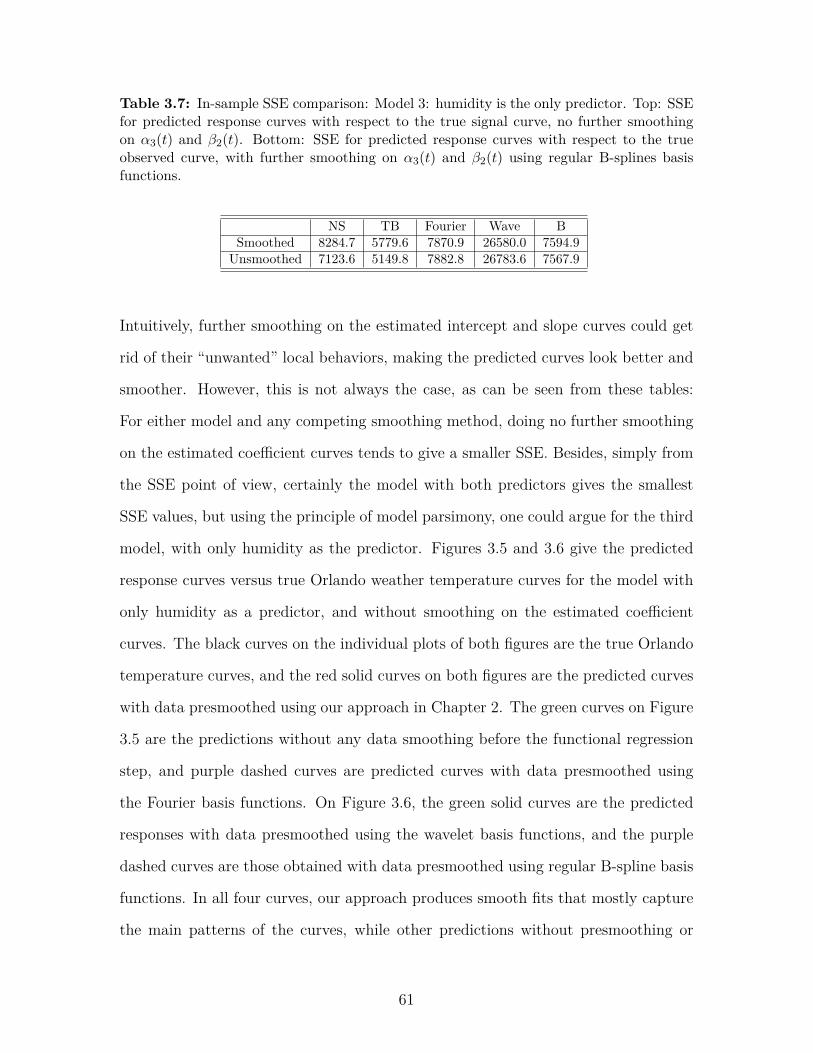
Table 3.7: In-sample SSE comparison: Model 3: humidity is the only predictor. Top: SSEfor predicted response curves with respect to the true signal curve, no further smoothingon α3(t) and β2(t). Bottom: SSE for predicted response curves with respect to the trueobserved curve, with further smoothing on α3(t) and β2(t) using regular B-splines basisfunctions.

NS TB Fourier Wave BSmoothed 8284.7 5779.6 7870.9 26580.0 7594.9

Unsmoothed 7123.6 5149.8 7882.8 26783.6 7567.9

Intuitively, further smoothing on the estimated intercept and slope curves could get

rid of their “unwanted” local behaviors, making the predicted curves look better and

smoother. However, this is not always the case, as can be seen from these tables:

For either model and any competing smoothing method, doing no further smoothing

on the estimated coefficient curves tends to give a smaller SSE. Besides, simply from

the SSE point of view, certainly the model with both predictors gives the smallest

SSE values, but using the principle of model parsimony, one could argue for the third

model, with only humidity as the predictor. Figures 3.5 and 3.6 give the predicted

response curves versus true Orlando weather temperature curves for the model with

only humidity as a predictor, and without smoothing on the estimated coefficient

curves. The black curves on the individual plots of both figures are the true Orlando

temperature curves, and the red solid curves on both figures are the predicted curves

with data presmoothed using our approach in Chapter 2. The green curves on Figure

3.5 are the predictions without any data smoothing before the functional regression

step, and purple dashed curves are predicted curves with data presmoothed using

the Fourier basis functions. On Figure 3.6, the green solid curves are the predicted

responses with data presmoothed using the wavelet basis functions, and the purple

dashed curves are those obtained with data presmoothed using regular B-spline basis

functions. In all four curves, our approach produces smooth fits that mostly capture

the main patterns of the curves, while other predictions without presmoothing or

61

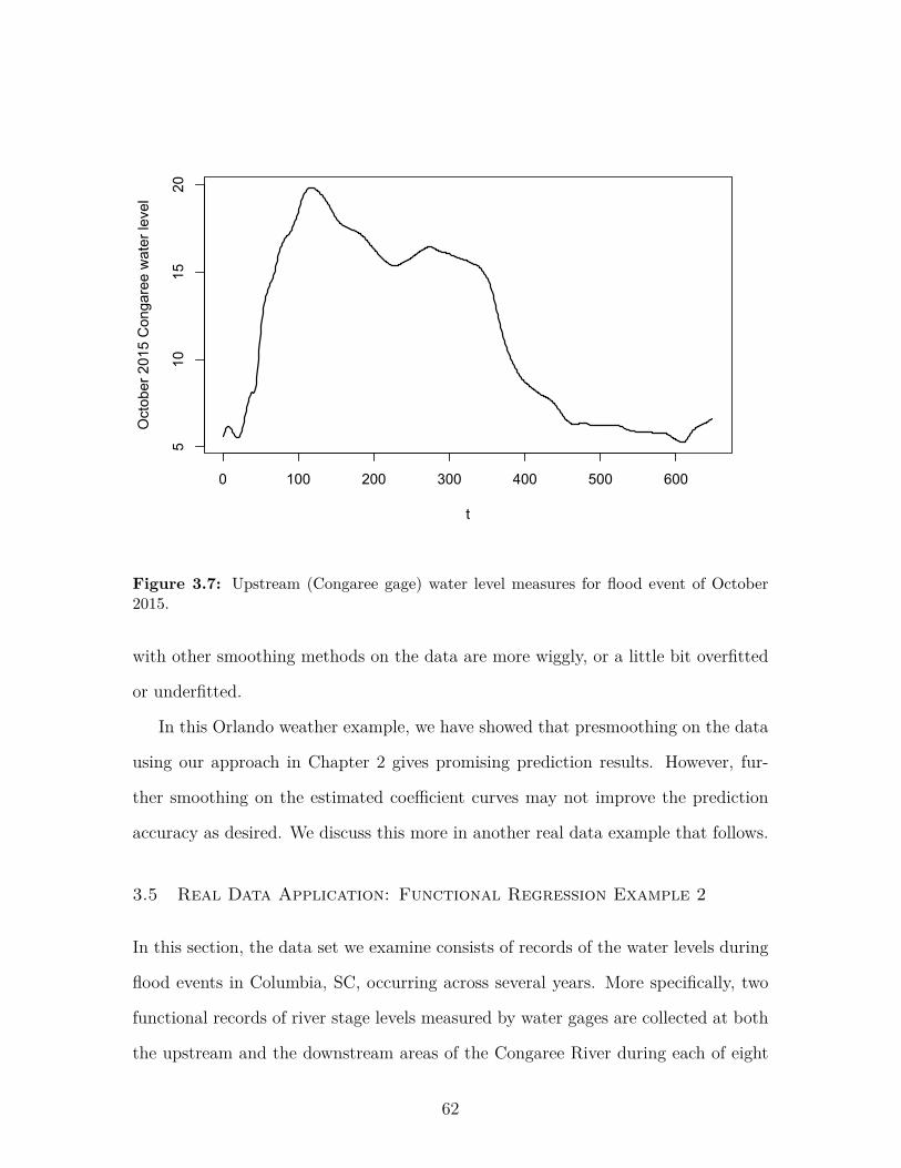
0 100 200 300 400 500 600

510

1520

t

Oct

ober

201

5 C

onga

ree

wat

er le

vel

Figure 3.7: Upstream (Congaree gage) water level measures for flood event of October2015.

with other smoothing methods on the data are more wiggly, or a little bit overfitted

or underfitted.

In this Orlando weather example, we have showed that presmoothing on the data

using our approach in Chapter 2 gives promising prediction results. However, fur-

ther smoothing on the estimated coefficient curves may not improve the prediction

accuracy as desired. We discuss this more in another real data example that follows.

3.5 Real Data Application: Functional Regression Example 2

In this section, the data set we examine consists of records of the water levels during

flood events in Columbia, SC, occurring across several years. More specifically, two

functional records of river stage levels measured by water gages are collected at both

the upstream and the downstream areas of the Congaree River during each of eight

62

0 100 200 300 400 500 600

02

46

810

12

t

Oct

ober

201

5 C

edar

Cre

ek w

ater

leve

l

Figure 3.8: Downstream (Cedar Creek gage) water level measures for flood event ofOctober 2015.

flood events between August 1995 and October 2015. Note that the “stage” is a

measurement of the height of the river’s water level at the location of the gage. We

call the upstream gage the Congaree gage (“Cong”), and downstream gage the Cedar

Creek gage (“Cedar”). For each flood event, the Congaree stage and the Cedar Creek

stage are measured at the same sequence of time points except for the last flood event,

which occurred in October 2015. As can be seen from Figure 3.7, the Congaree curve

corresponding to the October 2015 flood event has 648 stage readings from the start of

the measurements. The water level smoothly increases during the flood and gradually

drops to normal with a few wiggles after the event. The Cedar Creek curve for this

event is given in Figure 3.8; the response function (i.e., the water level) increases

gradually at the start of the flood event, yet takes a few rapid and almost straight

dips after the peak. And the gage readings were all missing afterwards.

63

Figure 3.9: Downstream (Cedar Creek gage) and upstream (Congaree gage) water levelmeasures for six flood events.

We would like to estimate the whole curve of stage readings at the downstream

gage. It is suspected that the gage lost readings due to being suddenly broken in

the flood, and the peak of the function seems to be the breaking point. Therefore

we keep only that portion of the curve up to the observed peak, and the rest of the

measurements will be considered missing.

If we standardize each curve to make each flood event of standard length, so that

each curve has the same number of time points, we obtain Figure 3.9 as follows. Six

pairs of Congaree and Cedar Creek water level curves for six flood events are drawn in

figure 3.9. And for each flood event, the Congaree curve and the Cedar Creek curve

are shown in the same color, and drawn with the same symbol type, with the upper

and lower ones representing the upstream and downstream water levels, respectively.

The number of time points in the time sequences for all flood events are standardized

64

to be 500 to make each curve have the same time vector. This implies that each time

interval [ti, ti+1) represents 1/500 of the total length of the time event.

Apparently for each flood event, the two observed functional curves seem to follow

roughly the same pattern. Thus we propose functional regression model between the

downstream and upstream water levels, with the former being the response of interest

and the latter being the predictor of the model, to see whether such a functional

relationship helps to predict the incomplete Cedar Creek water level curve of the

October 2015 flood event. We will also see whether our smoothing method provides

any improvement in the prediction accuracy when predicting the response curves.

The first model explored is the concurrent model as discussed earlier in the chap-

ter, since it is believed that the water levels at the Cedar Creek and Congaree areas

at the same time point should be related. Functional regression is initially carried

out on the set of seven pairs of raw observed data curves and the in-sample prediction

error is calculated. The α(t) and β(t) obtained are shown in Figure 3.10. The α(t)

and β(t) curves, up to a scale, seem to be mirroring effects of each other.

In Figure 3.11, the blue, red and green curve give the observed Congaree stage

values, the observed Cedar Creek stage values, and predicted Cedar Creek stage

values, respectively. The functional relationship seems fine for our data set based on

Figure 3.11. As can be seen from the predicted curves, the majority of the predicted

curves mimic the behavior of the truly observed Cedar Creek curves, with some

noticeable deviations observed for the first and the seventh flood events.

We wonder whether some of the local behavior shown in the predicted curves

in Figure 3.11 is extraneous, and thus the same procedure is carried out on the

smoothed functional curves. The curves are smoothed using smoothing splines, with

the smoothing parameter selected as 0.7. This was implemented using the R func-

tion smooth.spline. The α(t) and β(t) obtained using the smoothed response and

predictor curves are smoothed further using smoothing splines, with the smoothing

65

0 100 200 300 400 500

-20

-5

t

α(t)

0 100 200 300 400 500

0.5

1.5

t

β(t)

Figure 3.10: Functional regression based on raw data curves. Top: intercept functionα(t). Bottom: slope function β(t)

parameter value being 0.2, in order to capture only the major effects between the

response and the predictor curves. The smoothed α(t) and β(t) curves are given in

Figure 3.12. The smoothed α(t) and β(t), i.e., α(t) and β(t), obtained using smooth-

ing splines, are not perfect, since some of the major effects are dampened, yet it gives

the approximate overall effects of the intercept and the slope curves.

The predicted Cedar Creek stage levels based on the smoothed version of the

concurrent model are given in Figure 3.13. The curves look cleaner compared to

the unsmoothed version, yet the deviations in the predicted and the smoothed data

curves of the Cedar Creek area during the first, the sixth and the seventh flood events

are still apparent. SSE is also calculated for both settings. Table 3.8 gives detailed

66

0 100 200 300 400 500

0510

20

t

wat

er le

vel

0 100 200 300 400 500

0510

20

t

wat

er le

vel

0 100 200 300 400 500

0510

20

t

wat

er le

vel

0 100 200 300 400 500

0510

20

t

wat

er le

vel

0 100 200 300 400 500

0510

20

t

wat

er le

vel

0 100 200 300 400 500

0510

20

t

wat

er le

vel

0 100 200 300 400 500

0510

20

t

wat

er le

vel

Figure 3.11: Functional regression based on raw data curves. Blue dashed curve: ob-served Congaree curve. Green solid curve: observed Cedar Creek curve. Red dashed curve:predicted Cedar Creek curve.

comparison, it suggests that smoothing does provide improvement for functional re-

gression prediction accuracy.

Notice that we are doing in-sample predictions, and smoothing apparently pro-

vides some improvement in terms of the total sum of squared errors. Figure 3.14

shows the observed Cedar Creek and Congaree curves, along with the predicted Cedar

Creek curve for the flood event of October 2015. It is obvious that the predicted

curve roughly mimics the behavior of the observed Congaree curve, as does other

flood events. The predicted curve seems fine in the sense that it roughly follows the

67

0 100 200 300 400 500

-15

-5

t

α(t)

0 100 200 300 400 500

0.2

0.8

1.4

t

β(t)

Figure 3.12: Functional regression based on pre-smoothed data curves. Top: smoothedintercept α(t). Bottom: smoothed slope β(t)

Table 3.8: SSE comparison for seven flood events. Top: SSE values based on functionalregression without any smoothing. Bottom: SSE values based on functional regression withraw data curves and estimated intercept and slope curves smoothed via smoothing splines.

Aug1995 Feb2010 Mar2003 Mar2007 May2003 May2013 Sep2004Unsmoothed 1763.5 268.4 371.4 588.6 510.0 229.0 622.9Smoothed 1632.1 221.2 261.4 532.9 314.3 174.4 491.3

68

0 100 200 300 400 500

0510

20

t

wat

er le

vel

0 100 200 300 400 500

0510

20

t

wat

er le

vel

0 100 200 300 400 500

0510

20

t

wat

er le

vel

0 100 200 300 400 500

0510

20

t

wat

er le

vel

0 100 200 300 400 500

0510

20

t

wat

er le

vel

0 100 200 300 400 500

0510

20

t

wat

er le

vel

0 100 200 300 400 500

0510

20

t

wat

er le

vel

Figure 3.13: Functional regression based on pre-smoothed data curves, obtained interceptand slope curves are further smoothed for prediction. Blue dashed curve: smoothed Con-garee curve. Green solid curve: smoothed Cedar Creek curve. Red dashed curve: predictedCedar Creek curve.

observed Cedar Creek curve prior to the peak.

To assess whether the model predicted well for curves outside the sample, like the

October 2015 curve, we performed out-of-sample predictions by iteratively dropping

the pair of curves for one flood event at a time when carrying out the functional

regression. In other words, for each flood event, we excluded the pair of observed

curves for that specific event from our functional regression fitting, and predicted the

corresponding Cedar Creek curve of the flood event. Thus, we would have a slightly

different pair of α(t) and β(t) after deleting each event. See Figure 3.15 and Figure

69

0 100 200 300 400 500

05

1015

20

t

wat

er le

vel

Figure 3.14: Functional regression based on pre-smoothed data curves, obtained inter-cept and slope curves are further smoothed for prediction. Blue dashed curve: smoothedCongaree curve for October 2015 event. Green solid curve: smoothed Cedar Creek curvefor October 2015 event. Red dashed curve: predicted Cedar Creek curve for October 2015event.

70

0 100 200 300 400 500

0.0

1.0

2.0

t

β(t)

0 100 200 300 400 500

0.5

1.5

t

β(t)

0 100 200 300 400 500

0.5

1.5

t

β(t)

0 100 200 300 400 500

0.5

1.5

t

β(t)

0 100 200 300 400 500

0.0

1.0

2.0

t

β(t)

0 100 200 300 400 500

0.5

1.5

2.5

t

β(t)

0 100 200 300 400 500

0.5

1.5

t

β(t)

Figure 3.15: Obtained slopes for seven flood events using functional regression based onraw data curves using “Cross-validation” idea.

3.16 for the estimated slope curves based on cross-validated data sets. In particular,

Figure 3.15 gives slope curves for the functional regression based on unsmoothed re-

sponse and predictor curves, and Figure 3.16 gives those based on curves presmoothed

via smoothing splines. Further smoothing is applied to the obtained α(t) and β(t)

curves in the smoothed version to capture only the major patterns for prediction

purposes. The SSE comparisons are given in Table 3.9. It provides evidence that

smoothing enhances accuracy for both in-sample and out-of-sample predictions most

of the time.

Now we employ the same model, but all the curve fitting procedures are carried

71

0 100 200 300 400 500

0.5

1.5

t

β(t)

0 100 200 300 400 500

0.2

0.8

1.4

t

β(t)

0 100 200 300 400 500

0.2

0.8

1.4

t

β(t)

0 100 200 300 400 500

0.4

0.8

1.2

t

β(t)

0 100 200 300 400 500

0.00.51.01.5

t

β(t)

0 100 200 300 400 500

0.5

1.5

t

β(t)

0 100 200 300 400 500

0.2

0.8

1.4

t

β(t)

Figure 3.16: Obtained slopes for seven flood events using functional regression based onpre-smoothed data curves using “Cross-validation” idea.

Table 3.9: SSE comparison for seven flood events. SSE values based on functional re-gression without any pre-smoothing on the observation curves. “Cross-validation” idea isutilized to obtain out-of-sample predictions. Top: SSE values based on functional regressionwithout any smoothing. Bottom: SSE values based on functional regression with raw datacurves and estimated intercept and slope curves smoothed via smoothing splines.

Aug1995 Feb2010 Mar2003 Mar2007 May2003 May2013 Sep2004Unsmoothed 2986.1 452.9 924.6 1010.6 1020.7 2850.33 1294.1Smoothed 2654.5 359.8 776.3 874.3 518.8 2908.0 1011.3

72

Table 3.10: SSE comparison for seven flood events. SSE values based on functionalregression with Bayesian transformed B-splines method on the observed curves.

Aug1995 Feb2010 Mar2003 Mar2007 May2003 May2013 Sep20041953.8 333.4 780.5 507.7 569.3 404.2 471.9

out via our smoothing method proposed in Chapter 2. Note that in the following

discussions, we all have deleted a certain number of points on the two edges of each

of the observed curves, hoping to obtain better predictions with more magnified flood

event behaviors on the curves.

Firstly, considering the smoothed nature of the observed curves, especially the

Congaree curves, we choose to smooth them initially using order 4 basis functions

with 3 equally-spaced interior knots in our Bayesian transformed B-splines method.

The comparison plot of smoothed predictor curves, smoothed response curves

and predicted response curves is shown in Figure 3.17. In this scenario, we simply

smoothed the observed curves using our method proposed in Chapter 2, but did no

further smoothing on the obtained α(t) and β(t) curves.

The predicted curves seem to mimic the smoothed response very well except for

some local areas for the first flood event. And the SSE measures for the seven flood

events using this approach are given in Table 3.10. Comparison of the magnitudes

of SSE obtained using this approach with those SSE values obtained from using

roughness penalty based smoothing methods (Table 3.8) shows that the former is

superior to the latter in only two out of seven curves (i.e., the March 2007 event, and

the September 2004 event). But since the true signal curves are unknown, and thus

the SSE values in Tables 3.8 and 3.10 are calculated based on the predicted curves

with respect to the smoothed response curves using different methods of eliminating

noise in the observed curves, we would agree that these SSE values serve only as a

rough reference of the performances of competing approaches.

73

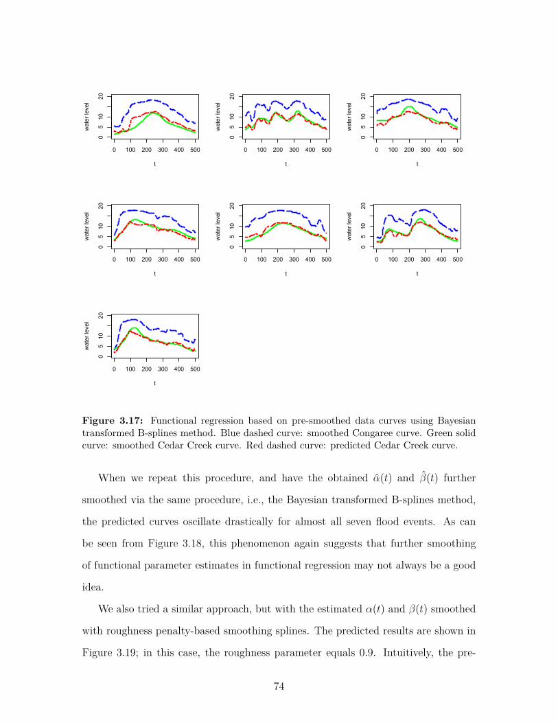
0 100 200 300 400 500

0510

20

t

wat

er le

vel

0 100 200 300 400 500

0510

20

t

wat

er le

vel

0 100 200 300 400 500

0510

20

t

wat

er le

vel

0 100 200 300 400 500

0510

20

t

wat

er le

vel

0 100 200 300 400 500

0510

20

t

wat

er le

vel

0 100 200 300 400 500

0510

20

t

wat

er le

vel

0 100 200 300 400 500

0510

20

t

wat

er le

vel

Figure 3.17: Functional regression based on pre-smoothed data curves using Bayesiantransformed B-splines method. Blue dashed curve: smoothed Congaree curve. Green solidcurve: smoothed Cedar Creek curve. Red dashed curve: predicted Cedar Creek curve.

When we repeat this procedure, and have the obtained α(t) and β(t) further

smoothed via the same procedure, i.e., the Bayesian transformed B-splines method,

the predicted curves oscillate drastically for almost all seven flood events. As can

be seen from Figure 3.18, this phenomenon again suggests that further smoothing

of functional parameter estimates in functional regression may not always be a good

idea.

We also tried a similar approach, but with the estimated α(t) and β(t) smoothed

with roughness penalty-based smoothing splines. The predicted results are shown in

Figure 3.19; in this case, the roughness parameter equals 0.9. Intuitively, the pre-

74

0 100 200 300 400 500

0510

20

t

wat

er le

vel

0 100 200 300 400 500

0510

20

t

wat

er le

vel

0 100 200 300 400 500

0510

20

t

wat

er le

vel

0 100 200 300 400 500

0510

20

t

wat

er le

vel

0 100 200 300 400 500

0510

20

t

wat

er le

vel

0 100 200 300 400 500

0510

20

t

wat

er le

vel

0 100 200 300 400 500

0510

20

t

wat

er le

vel

Figure 3.18: Functional regression based on pre-smoothed data curves using Bayesiantransformed B-splines method. Obtained α(t) and β(t) curves are further smoothed usingthe same procedure. Blue dashed curve: smoothed Congaree curve. Green solid curve:smoothed Cedar Creek curve. Red dashed curve: predicted Cedar Creek curve.

diction accuracy would be expected to be higher when using the same smoothing

method on both the original observed curves and the estimated functional regression

coefficient curves. However, apparently the predicted curves are smoother and more

accurate with this approach. As can be seen from Figure 3.19, the prediction perfor-

mances are superior to those obtained by using our method for smoothing on α(t)

and β(t) (Figure 3.18).

We showed in Chapter 2 that our proposed method tends to be more flexible

than several currently popular regression spline fitting methods. We thus wonder

75

0 100 200 300 400 500

0510

20

t

wat

er le

vel

0 100 200 300 400 5000

510

20

t

wat

er le

vel

0 100 200 300 400 500

0510

20

t

wat

er le

vel

0 100 200 300 400 500

0510

20

t

wat

er le

vel

0 100 200 300 400 500

0510

20

t

wat

er le

vel

0 100 200 300 400 500

0510

20t

wat

er le

vel

0 100 200 300 400 500

0510

20

t

wat

er le

vel

Figure 3.19: Functional regression based on pre-smoothed data curves using Bayesiantransformed B-splines method. Obtained α(t) and β(t) curves are further smoothed usingsmoothing splines with roughness penalty parameter = 0.9. Blue dashed curve: smoothedCongaree curve. Green solid curve: smoothed Cedar Creek curve. Red dashed curve:predicted Cedar Creek curve.

76

Table 3.11: SSE comparison for seven flood events. SSE values based on functionalregression with Bayesian transformed B-splines method on the observation curves. Top: Nofurther smoothing on α(t) and β(t) curves. Middle: α(t) and β(t) curves further smoothedusing smoothed splines with roughness parameter = 0.9. Bottom: α(t) and β(t) curvesfurther smoothed using smoothed splines with roughness parameter = 0.5.

Flood Aug1995 Feb2010 Mar2003 Mar2007 May2003 May2013 Sep2004Unsmoothed 1953.8 333.4 780.5 507.7 569.3 404.2 471.9

Smoothed (0.9) 2139.1 585.8 762.0 514.4 642.6 556.1 496.6Smoothed (0.5) 1966.4 341.6 780.6 508.0 569.4 418.4 473.9

whether a roughness-penalty-based smoothing method is performing better than our

proposed approach, and whether this has resulted in its superior prediction accuracies

and smoothness.

The plots that compare the original estimated α(t) and β(t) curves with the ones

smoothed with our method from Chapter 2 and with smoothing splines are given in

Figures 3.20 and 3.21. The smoothed intercept and slope curves obtained with our

method seem fine in terms of curve fitting. Some minor local noise-type behaviors are

successfully removed, while a relatively accurate fit is maintained. On the other hand,

the other curves are severely under-fitted. Thus we conclude the prediction accuracy

for functional regression models may not be directly related to the smoothing accuracy

of the estimated intercept and slope curves.

Table 3.11 gives the calculated SSE values for α(t) and β(t) smoothed using

smoothing splines with roughness penalty parameter being 0.9 and 0.5, versus no

further smoothing on them. Notice that for roughness penalty values of 0.9 and 0.5,

the SSE values do not differ too much for four out of seven flood events. In other

words, no matter which roughness penalty value is utilized, the predicted curves are

always relatively stable. The reason for the wiggly nature of the predicted curves via

our method and the stability in those obtained via smoothing splines is somewhat

uncertain. Note that in Figure 3.18, several minor oscillations exist across the entire

time axis for all seven flood events, and more specifically, there appear to be sharp

77

0 100 200 300 400 500

-20

-55

t

α(t)

0 100 200 300 400 500

0.5

1.5

t

β(t)

Figure 3.20: Estimated α(t) and β(t) curves smoothed using Bayesian transformed B-splines method. Top: estimated (black) and smoothed (red) α(t) curve. Bottom: estimated(black) and smoothed (red) β(t) curve.

valleys at around time point 100 in the predicted curves for each of them. On the other

hand, a close look at Figure 3.20 reveals that both α(t) and β(t) have an obvious local

event at exactly the same location of around the 100th time point. And that this local

event is described well for the α(t) curve, yet the same procedure underestimates the

peak at the same location for β(t). Therefore the conjecture is that the estimated α(t)

and β(t) curves are intrinsically of different smoothness levels, and our method adapts

well to fitting the overall shapes of the original curves. Thus with curves of vastly

different intrinsic roughness, our method fits the two curves to different smoothness

levels, even with the same number of basis functions. And even though some of these

discrepancies may seem unnoticeable from a smoothing point of view, their effects are

78

0 100 200 300 400 500

-20

-55

t

α(t)

0 100 200 300 400 500

0.5

1.5

t

β(t)

Figure 3.21: Estimated α(t) and β(t) curves smoothed using smoothing splines methodwith roughness penalty parameter = 0.9. Top: estimated (black) and smoothed (red) α(t)curve. Bottom: estimated (black) and smoothed (red) β(t) curve.

magnified in applications such as regression predictions. On the other hand, when

using traditional smoothing methods, such as regression splines or smoothing splines,

as long as one utilizes the same number of basis functions, same knot locations, and

chooses the same roughness penalty parameter values when smoothing those curves,

the set of resulting curves would always have the same smoothness level, no matter

how rough or smooth the original curves might be. In fact, a close look at Figure

3.21 reveals that even though the α(t) and β(t) curves are both severely under-fitted,

they are under-fitted to the same extent, and thus when doing predictions, the under-

fitting effect evened out, leaving the predicted curve unaffected by the inaccuracy of

the smoothing of the intercept and slope. This can be verified by looking at the

79

0 100 200 300 400 500

0510

20

t

wat

er le

vel

0 100 200 300 400 500

0510

20

t

wat

er le

vel

0 100 200 300 400 500

0510

20

t

wat

er le

vel

0 100 200 300 400 500

0510

20

t

wat

er le

vel

0 100 200 300 400 500

0510

20

t

wat

er le

vel

0 100 200 300 400 500

0510

20

t

wat

er le

vel

0 100 200 300 400 500

0510

20

t

wat

er le

vel

Figure 3.22: Functional regression based on pre-smoothed data curves using the Bayesiantransformed B-splines method. Obtained ˆα(t) and ˆβ(t) curves are further smoothed usingsmoothing splines with roughness penalty parameters = 0.9 (α(t)) and 0.5 (β(t)). Bluedashed curve: smoothed Congaree curve. Green solid curve: smoothed Cedar Creek curve.Red dashed curve: predicted Cedar Creek curve.

prediction performance when using traditional smoothing splines to smooth α(t) and

β(t), with different roughness penalty values.

Figure 3.22 gives predicted “Cedar” and smoothed “Cedar” and “Cong” curves

when data are pre-smoothed using the Bayesian transformed basis functions approach,

and the obtained α(t) curve further smoothed with smoothing splines using roughness

penalty parameter = 0.9, and β(t) curve smoothed with the same procedure, but with

roughness penalty parameter = 0.5. In this figure, all predicted Cedar Creek curves

80

0 100 200 300 400 500

-20

-55

t

α(t)

0 100 200 300 400 500

0.5

1.5

t

β(t)

Figure 3.23: Estimated α(t) and β(t) curves smoothed using smoothing splines methodwith roughness penalty parameter = 0.9 (α(t)) and 0.5 (β(t)). Top: estimated (black) andsmoothed (red) α(t) curve. Bottom: estimated (black) and smoothed (red) β(t) curve.

look poor and follow similar patterns, no matter what the shapes of the original

curves might be. In particular, there are spikes at around the 100th, the 280th, the

320th time points in all of them. Apparently, the intercept and slope curves are fitted

to different smoothness levels at those corresponding areas, which implies that the

patterns in the predicted curves are dominated by the shapes of the smoothed α(t)

and β(t) curves. Whenever these are not smoothed to the same amount, unwanted

behaviors at those corresponding local areas is seen.

Table 3.11 seems to have suggested that no further smoothing on α(t) and β(t)

would give the optimal prediction result, no matter what method we use (i.e., trans-

formed B-splines, or smoothing splines) to smooth the original observed curves. Yet

81

Table 3.12: SSE comparison for seven flood events. SSE values based on functionalregression with Bayesian transformed B-splines method on the observation curves. “Cross-validation” idea is utilized to obtain out-of-sample predictions. Top: No further smoothingon α(t) and β(t) curves. Bottom: α(t) and β(t) curves further smoothed using smoothedsplines with roughness parameter = 0.9.

Flood Aug1995 Feb2010 Mar2003 Mar2007 May2003 May2013 Sep2004Unsmoothed 2892.6 764.8 1592.8 925.2 977.4 3411.7 1122.3Smoothed 2870.1 833.6 1377.6 770.0 910.8 1918.3 808.1

if we carry out the same functional regression procedure by using cross-validated data

sets as described above, we can see that for out-of-sample prediction, smoothing does

help with prediction accuracy. Since the prediction performances are more stable

when using the smoothing splines method to further smooth α(t) and β(t), we com-

pare its performance with the case when no further smoothing is applied in Figures

3.24 and 3.25. Apparently, without further smoothing, the predicted curves are more

prone to local oscillations, whereas the curves are smoother and lack unnecessary

fluctuations when smoothing is performed on α(t) and β(t). Table 3.12 gives detailed

SSE values for the two competing methods.

We have also investigated an interaction model which includes the first deriva-

tive function of the predictor and the interaction of the derivative function and the

predictor function as two extra functional covariates. Since the model’s prediction

performance is instable due to extreme values in the derivative curves, we omit any

further discussion here.

In sum, we conclude that using smoothing splines as the major fitting method on

the observed curves before functional regression, and further smoothing the obtained

α(t) and β(t) afterwards using smoothing splines, gives the most stable and accurate

prediction result. In particular, the roughness parameter values selected to smooth

the estimated intercept and slope curves must be the same to produce a desirable

result. See Figure 3.14 for a sample prediction of the “Cedar” stage for the October

82

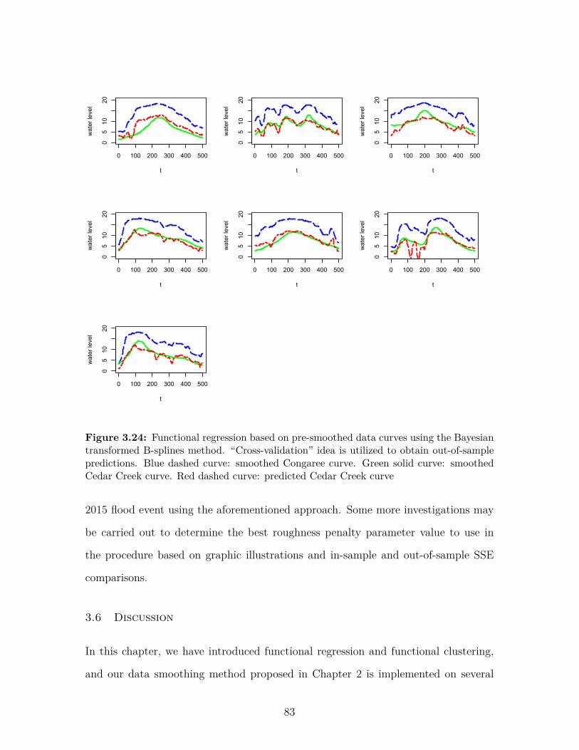
0 100 200 300 400 500

0510

20

t

wat

er le

vel

0 100 200 300 400 500

0510

20

t

wat

er le

vel

0 100 200 300 400 500

0510

20

t

wat

er le

vel

0 100 200 300 400 500

0510

20

t

wat

er le

vel

0 100 200 300 400 500

0510

20

t

wat

er le

vel

0 100 200 300 400 500

0510

20

t

wat

er le

vel

0 100 200 300 400 500

0510

20

t

wat

er le

vel

Figure 3.24: Functional regression based on pre-smoothed data curves using the Bayesiantransformed B-splines method. “Cross-validation” idea is utilized to obtain out-of-samplepredictions. Blue dashed curve: smoothed Congaree curve. Green solid curve: smoothedCedar Creek curve. Red dashed curve: predicted Cedar Creek curve

2015 flood event using the aforementioned approach. Some more investigations may

be carried out to determine the best roughness penalty parameter value to use in

the procedure based on graphic illustrations and in-sample and out-of-sample SSE

comparisons.

3.6 Discussion

In this chapter, we have introduced functional regression and functional clustering,

and our data smoothing method proposed in Chapter 2 is implemented on several

83

0 100 200 300 400 500

0510

20

t

wat

er le

vel

0 100 200 300 400 5000

510

20

t

wat

er le

vel

0 100 200 300 400 500

0510

20

t

wat

er le

vel

0 100 200 300 400 500

0510

20

t

wat

er le

vel

0 100 200 300 400 500

0510

20

t

wat

er le

vel

0 100 200 300 400 500

0510

20t

wat

er le

vel

0 100 200 300 400 500

0510

20

t

wat

er le

vel

Figure 3.25: Functional regression based on pre-smoothed data curves using the Bayesiantransformed B-splines method. Obtained α(t) and β(t) curves are further smoothed usingsmoothing splines method with roughness penalty parameter = 0.9. “Cross-validation” isutilized to obtain out-of-sample predictions. Blue dashed curve: smoothed Congaree curve.Green solid curve: smoothed Cedar Creek curve. Red dashed curve: predicted Cedar Creekcurve

84

simulated data or real data examples. We have showed from our analysis results that

in most scenarios, our smoothing method is useful in improving statistical estimation

quality such as prediction or clustering accuracies. And our approach leads to greater

improvement in several of the scenarios compared to some other smoothing methods

such as the regular B-spline basis approach, the spline approach with specified knots,

the wavelet basis, or the Fourier basis smoothing methods. However, it is also seen

from previous examples that in certain circumstances, unexpected results may occur,

since functional data smoothing accuracy and prediction or clustering accuracies are

different objectives. Hence it is not guaranteed that better data smoothing will

always lead to better prediction performance. In particular, in some cases, too much

smoothing (i.e., presmoothing the raw data, then smoothing the estimated coefficient

curves after functional regression) may not always lead to improvement. Hence, it

is important that one does enough in-sample and out-of-sample analysis to compare

smoothing versus no smoothing, and to compare different smoothing methods, before

determining the appropriate approach for the specific problem at hand.

85

Chapter 4

Sparse functional data fitting with

transformed spline basis

Summary: In this Chapter, we will extend our functional data smoothing method

proposed in Chapter 2 to the sparse data scenario. Our warping function is applied

to the joint time interval for a cluster of curves that are similar in nature, and the

Bayesian framework is imposed on the fitting method to have the algorithm learn

from data to produce the “optimal” transformation of time.

4.1 Introduction

Recall that in chapter 2, we proposed an automatic functional data fitting method

that can be applied to a group of data curves of various shapes without pre-screening

the curves and selecting the appropriate basis functions for fitting them one by one.

We then showed via various simulations and real data analysis results that our pro-

posed method gives competitive fitting accuracy when compared with the pool of

currently popular regression spline smoothing methods.

However, one assumption we made in order to have our proposed method produce

desirable fitting results is that we require all the raw data curves to be originally

observed over a fine grid of time points on the continuous domain T , say, roughly 100

time points for a time interval of [0, 1]. In other words, we have to have a sufficient

amount of observed information within each unit time interval to be able to perform

the proposed method in Chapter 2 and obtain good smoothing results in terms of

86

fitted curve smoothness and accuracy (as measured by both SSE with respect to the

raw curve and SSE with respect to the true signal curve). This assumption is vital

because it allows us to use simple linear interpolation between each pair of adjacent

fitted values, which are obtained from the Bayesian model we built, to achieve a fitted

curve that reveals a relatively accurate depiction of the true shape of the curve itself.

In this sense, we essentially treat a group of curves as independent from each other,

and the fitting procedure is carried out on the curves one by one. Thus if the original

curves are truly spiky, then our method proposed in Chapter 2 suffices to fit the spikes

well. On the other hand, if the original curves are intrinsically smooth, then using

our method will also produce a relatively smooth fitted curve. Hence, under such

an assumption, we can confidently claim that our method performs competitively in

terms of producing accurate fitted functional curves, and that it is especially useful

for fitting irregularly shaped and spiky curves.

When this assumption is relaxed, or in other words, when functional data are

observed only at a set of sparsely located time points, then our proposed method

may result in undesirable behavior, such as unwanted spikes and loss of smoothness.

That is again due to the use of linear interpolation between each pair of adjacent

fitted values in the final step. Blindly using linear interpolation when there is not

sufficient information contained within each unit length of time produces undesirable

and extreme spikes when the true underlying functional form may be smooth. As a

result, we would need some other method to accommodate the lack of information in

circumstances when the data are only observed at a sparse set of time points.

In sum, our goal for this chapter is to extend our method proposed in Chapter 2

to the sparse data scenario, and we must overcome the following obstacles:

• Fitting curves one by one may no longer be feasible, since each curve itself carries

information that is too limited with respect to its true underlying functional

form, and hence fitting results could be poor.

87

• We want the resulting fitted curves to be smooth and to accurately depict the

nature of the true underlying functional form of the curves even when the data

is only measured sparsely. As a result, either linear interpolation should be

abandoned in the final step of the procedure, or some other accommodations

need to be made to ensure fitting smoothness and accuracy.

Our approach proposed here is inspired by Thompson and Rosen (2008), in which

the authors have discussed a Bayesian approach for fitting sparse functional data.

Note that one vital assumption for this approach to succeed is that there has to be

a cluster of curves that share the same true underlying baseline function, so that the

information from the entire set of curves could be utilized jointly in some way in order

to achieve a better estimate. Hence, curves vary from each other as a direct result of

each curve’s individualized variation plus noise, where the former source of variation

is similar to the variation among factor effects in an ANOVA model. An example for

such a scenario would be a group of girls’ growth velocity curves. In general, all girls

should follow the same growing pattern, thus intuitively, there should be a common

trend of growth for all of them, yet each individual girl may have her own timings in

terms of growth “peaks” and “valleys”, due to factors such as nutrition level, general

environment, financial situations of their families, etc. Hence a common baseline

mean curve, and a individualized “factor effect” curve should both be included in the

mean function of an individual. Note that even though the cluster of curves need

to share the same baseline mean function, each individual curve does not need to be

measured on the same set of time points, they may not even need to share the same

minimal and maximal measured time points. That is due to the nature of the study

in practice. For instance, some girls’ growth curves might be recorded starting from

infancy, while some others may enter the study when they are already 6 or 7 years

old.

In the sections that follow, we will start with discussion of the general structure

88

of the method proposed in Thompson and Rosen (2008), along with our innovations

to the method that incorporate the transformed B-spline basis functions. We then

describe how we adapt our approach to the sparse functional data scenario to make

our method capable of producing a fit that balances smoothness and accuracy.

4.2 Bayesian Model Fitting for Sparse Functional Curves

Assume that a cluster of n individual functional curves, yj(t), j = 1, . . . , n, are each

observed at a set of sparsely located time points tj, where tj is the vector of sparse

time points measured for curve j, with length lj; thus the vector tj and its length are

allowed to vary from curve to curve. Note that all yj(t)’s are generated from the same

underlying grand mean function µ(t), and each curve has its own individual effect

function fj(t), for j = 1, 2, . . . , n. In other words, each observed curve is related to

its mean function via the following equation:

yj(t) = µ(t) + fj(t) + εj(t),

for t ∈ tj. Here εj(t) is the error term for curve j evaluated at time t, for j =

1, 2, . . . , n. Our goal for sparse functional data fitting is to study the common mean

function µ(t) and the individual signal function fj(t).

One way of fitting yj(t) is by using the B-spline basis functions. Thompson and

Rosen (2008) assumed that a common set of B-spline basis functions of the same

order and dimension can be used to describe both µ(t) and fj(t). That is, for a given

set of B-spline basis functions {B1(·), · · · , Bnb(·)} of dimension nb spanned on time

interval [0, TM ], where TM is the maximal measured time point among all curves, the

model assumed is:

yj(t) =nb∑k=1

βkBk(t) +nb∑k=1

bjBk(t) + εj(t),

here β = (β1, . . . , βnb)’ is the vector of coefficients related to the grand mean por-

tion of each curve, and bj = (b1j, . . . , bnbj)’ is the vector of coefficients related to

89

the mean contribution of the jth curve effect. However, even though B-spline basis

functions are most commonly used for fitting functional data, and have proved to be

flexible in their adaption to various shapes of functional curves, it is also well known

that the flexibility comes from the knots, which are used as joining points in the set

of B-splines. The fitting performance of using B-spline basis functions may not be

desirable unless the number and the locations of the knots are wisely selected. As ex-

pected, Thompson and Rosen (2008) incorporated the knot selection of B-spline basis

functions along with the parameter estimation in their Bayesian model. However, it

is shown in the simulation section of Chapter 2 that even with optimally selected

knots, sometimes the performance of B-splines may not improve on the transformed

B-splines we proposed. That is because the flexibility of the time transformation has

exempted us from the trouble of knot selection, and furthermore, the additional flex-

ibility we have gained from transforming the time interval has enabled our method to

produce an even more accurate fit than those obtained by using competing methods.

Hence, for the sparse data scenario, we once again assume that there exists some

underlying transformed B-spline basis functions, rather than a given set of B-spline

basis functions with flexible knot placement, as being the “true” basis functions for

curve fitting. Here “true” basis functions refer to “optimally” transformed basis func-

tions that are capable of producing a desirable fit with respect to smoothness and

accuracy. Hence, our goal is to somehow find the optimal transformation of time, in

order to produce the set of true basis functions.

To illustrate the idea, we again define Φ(tj) to be the design matrix we could

obtain by evaluating the aforementioned set of traditional B-spline basis functions

Bk(·)’s at time vector tj, where each column in the matrix isBk(tj), for j ∈ {1, 2, . . . , n}

and k ∈ {1, 2, . . . , nb}, and define the target, i.e., “optimally transformed design ma-

trix”, as Φ∗(tj), similarly as we did in Chapter 2. In other words, the model proposed

90

in Thompson and Rosen (2008) is:

yj(tj) = Φ(tj)β + Φ(tj)bj + εj(tj),

and the “true” model we assume is as follows:

yj(tj) = Φ∗(tj)β + Φ∗(tj)bj + εj(tj),

where j = 1, 2, . . . , n.

Now, our goal has been reduced to studying the nature of Φ∗(·), or more specifi-

cally, the quantification of the transformation on Φ(·), along with estimation of the

corresponding coefficient vectors β and bj. In order to achieve some transformation

of time and to transform Φ(·), we may employ the same technique utilized in Chapter

2, i.e., the time warping idea. And in order to obtain the “optimal” transformation

on time to produce Φ∗(·), and estimate the corresponding coefficients vectors β and

bj, we again use a Bayesian method.

For the purpose of illustration, we keep most of the notation used in Chapter

2. Note that even though we might not know how to “optimally” transform the

time interval at first, we might easily obtain some transformation of time by using

the warping idea. Similarly as we did in Chapter 2, before carrying out the fitting

procedure on the group of curves, we standardize the time interval of the curves. Note

that in Chapter 2, we standardize the observed time sequence for each curve, so that

each curve has a minimum measured time point 0 and a maximum time point 1, and

hence the standard method introduced in Chapter 2 can be applied to the curves one

by one. Here we want to utilize the information contained in the cluster of curves as

a whole, since each individual functional observation contains too little information

about the shape of itself. As a result, instead of standardization for each curve, we

view the set of time points for all curves as a whole, and standardize the whole set

of time points, so that after standardization, the entire set of time points measured,

{t1, t2, . . . , tn}, has a minimum value of 0 and a maximum value of 1. Hence now,

91

when we transform the time interval [0, 1], multiple curves are simultaneously affected.

Instead of defining some parametric continuous warping function on time, we may

simulate some “warped” time sequence tw first, and regard it as a transformation of

some monotone time vector T on [0, 1], and hence the transformation Φ(·) 7−→ Φ∗(·)

could be defined based on the relationship between the warped time sequence tw and

the original time vector T. To recap the idea, each curve in the cluster is measured on

a sequence of time points between 0 and 1 (that may not include 0 or 1). Assume that

we want to apply warping on a time sequence T, whose elements are (M + 1) equally

spaced points on the time interval [0, 1], including 0 and 1. We may obtain some

warped time sequence tw by generating a vector of length M , p = (p1, . . . , pM)′ from

the Dirichlet distribution, where each element in p can be viewed as the “jumps” in a

stepwise CDF function, since each element in p is positive, and the vector sums to 1.

In this sense, tw = {0, p1,∑2i=1 pi, . . . ,

∑M−1i=1 pi, 1} is a warped time sequence, due to

the facts that each element in the sequence is nonnegative, and they are in monotone

order. We have a given set of B-spline basis functions of dimension nb, and so one

may generate nb Dirichlet realizations of lengthM , denoted as TW = {tw1, . . . , twnb},

so that the original time sequence T for each of the nb basis functions is transformed

differently into {tw1, . . . , twnb}. In order to define the transformation from Φ(·) to

Φ∗(·), we again make the same assumption as in Chapter 2, i.e.,

Φ(T) = Φ∗(TW),

where on the left hand side, all nb basis functions are evaluated at the same original

time vector T, and on the right hand side, the kth basis function is evaluated on the

kth transformed time vector twk, for k = 1, 2, . . . , nb. As a result, back interpolation

can be applied directly to obtain Φ∗(T). But note that in the discussion above, we

have only described one way to transform the time sequence. We have not claimed,

however, that it is the “optimal” transformation we want. In fact, similarly as in

Chapter 2, a Bayesian model can be applied to the time transformation scheme, so

92

that the system can learn from the data and update the transformations of the time

sequences for each basis function from each iteration to the next, until it reaches

some balance, i.e., relatively stable shapes of the set of transformed basis functions.

We assume normal errors across different curves in the Bayesian framework. In other

words, our model is in fact:

yj(tj) = Φ∗(tj)β + Φ∗(tj)bj + εj(tj),

where

εj(tj) ∼ N(0, σ2ε I).

This model can also be interpreted as a mixed model as commonly used in longi-

tudinal studies, as pointed out by Thompson and Rosen (2008). The Φ∗(tj)β part

plays the role of the fixed effect in a mixed model, whereas Φ∗(tj)bj can be inter-

preted as the random effects portion of the jth curve. In other words, the random

coefficient terms bj are centered at 0, and have a variance-covariance matrix of Σb,

describing the within curve correlation between different measurement points. Here

the subscript b refers to the fact that Σb is the common variance-covariance matrix

for bj,∀j = 1, 2, . . . , n.

Now we have the following list of parameters of interest: β, b1,b2, . . . ,bn, σ2ε ,

p1,p2, . . . ,pnb , and Σb, where nb denotes the number of basis functions utilized in the

procedure. Our prior specifications are very similar to those employed in Thompson

and Rosen (2008), except that their method requires selection of knots in order to

achieve enough flexibility for the set of pre-specified B-spline basis functions. As we

have discussed in Chapter 2, one way to select knots is to incorporate the number and

locations of the knots into the Bayesian model, and have the data select those values

for us, since both the size and the placement of the pool of knots play important

roles in the shape of the B-spline basis functions. Thompson and Rosen (2008) took

a slightly simpler approach by starting from a large pool of pre-specified knots located

93

across the time axis, and they selected the knots from the initial pool by adding an

indicator variable to each of the knots. The total number of B-spline basis functions,

however, is also updated in each iteration in the MCMC. As we have discussed earlier,

the use of the time warping concept in our approach has played a similar role as knot

selection, and thus no dimension variation in the simulation step is needed.

Similar to Thompson and Rosen (2008), we combine bj and β in our model, by

assigning b∗j = bj + β a prior distribution with a mean of β. That is,

b∗j |Σb∗ ,β ∼MVN(β,Σb∗)

and

β ∼MVN(0, cI)

for j ∈ 1, 2, . . . , n. Note that here we use b∗j to refer the sum of the common mean

coefficients β and individual coefficients for the jth curve, bj, for j = 1, 2, . . . , n. And

we use b∗ to denote the joint information of {b∗1,b∗2, . . . ,b∗n}. We also change all the

corresponding subscripts in our notations. Hence our model can be rewritten as

yj(tj) = Φ∗(tj)b∗j + εj(tj),

where the hyperparameter c is chosen via some data-driven method, which we will

discuss later. Each vector pj of length M used to create a warped time sequence is

assigned a Dirichlet prior with hyperparameters a1, a2, . . . , aM . And lastly,

Σb∗ ∼ IW (η, S),

σ2ε ∼ IG(cε, dε),

where IW (·, ·) and IG(·, ·) denote the inverse Wishart and Inverse Gaussian distri-

butions, respectively. ηS is the scale matrix, and η is the degree of freedom for the

inverse Wishart distribution, and cε and dε are the shape and rate parameters for the

94

inverse gamma distribution, respectively. Again, the selection of values for hyperpa-

rameters S, η, cε and dε will be discussed later. Now we have specified the priors for

all parameters of interest.

We now consider the joint posterior distribution. For notational convenience when

we write the posterior, for now on, suppose that Y denotes the joint information in

all n curves, i.e., {y1(t1), y2(t2), . . . , yn(tn)}, and P denotes the joint information of

{p1,p2, . . . ,pnb}. Let L = ∑nj=1 lj, where lj is the length of discretized curve j.

Note also that each curve is measured on a possibly different time vector tj, so that

the transformed design matrix Φ∗(·) is only measured on tj for curve j, resulting in

Φ∗(tj). Then the joint posterior distribution for all parameters of interest is:

π(β,b∗, σ2ε ,Σb∗ ,P|Y)

∝ f(Y|b∗, σ2ε ,P) · f(b∗|Σb∗ ,β) · f(β) · f(Σb∗) · f(σ2

ε ) · f(P)

∝ σ−Lε exp{− 1

2σ2ε

n∑j=1

(yj(tj)−Φ∗′(tj)b∗′

j )(yj(tj)−Φ∗(tj)b∗j)}

× |Σb∗ |−n2 exp

{−1

2

n∑j=1

(b∗j − β)′Σ−1b∗ (b∗j − β)

}

× c−nb2 exp

{− 1

2cβ′β

}(σ2

ε )−(cε+1) exp{− dεσ2ε

}

× |Σb∗ |−(η+nb+1)

2 exp{−η

2 trace(sΣ−1b∗ )

}∏nbj=1

∏Mi=1 p

ai−1ij .

Here pij is the ith element in the vector pj. To use MCMC to simulate from the joint

posterior distribution, we follow the sampling scheme described below. Note that we

use superscripts [r] to denote parameter values generated for the rth iteration.

Step 0: Obtain initial values p[0]1 ,p

[0]2 , . . . ,p[0]

nb, σ2[0]

ε and Σ[0]b∗ by generating from

their prior distributions, with specified hyperparameter values. Obtain β[0] from a

random realization of f(β), and obtain b∗[0]j for all j = 1, . . . , n. by generating from

the prior distribution f(b∗j |β[0],Σ[0]b∗).

Then for iteration r:

95

Step 1: Generate σ2[r]ε from its conditional posterior distribution

f(σ2ε |Σ

[r−1]b∗ ,b∗[r−1],β[r−1],P[r−1],Y).

Step 2: Generate Σ[r]b∗ from its conditional posterior distribution

f(Σb∗|σ2[r]ε ,b∗[r−1],β[r−1],P[r−1],Y).

Step 3: Generate b∗[r] and β[r] jointly by sampling from f(b∗j ,β|Σ[r]b∗ , σ

2[r]ε ,P[r−1],Y)

for all j using the following factorization:

f(b∗j ,β|Σb∗ , σ2ε ,P,Y) ∝ f(b∗j |β, σ2

ε ,Σb∗ ,P,Y) · f(β|σ2ε ,Σb∗ ,P,Y).

Step 4: Generate P[r] by using the Metropolis-Hastings algorithm with a truncated

normal proposal distribution (similar to the technique used in Chapter 2).

The conditional distribution of (σ2ε | other parameters) is:

f(σ2ε |Σb∗ ,b∗,β,P,Y)

∝ σ−L−2(cε+1)ε exp

{− dεσ2ε

}

× exp{− 1

2σ2ε

n∑j=1

(yj(tj)−Φ∗(tj)b∗j)′(yj(tj)−Φ∗(tj)b∗j)}.

It is not hard to see that

σ2ε |∑

b∗ ,b∗,β,P,Y ∼ IG

(cε + L

2 , dε + 12

n∑j=1

(yj(tj)−Φ∗(tj)b∗j)′(yj(tj)−Φ∗(tj)b∗j)).

Next, the conditional posterior distribution of (Σb∗| other parameters) is:

P (Σb∗|σ2ε ,b∗,β,P,Y)

∝ |Σb∗ |−η+nb+1

2 exp{−1

2

n∑j=1

(b∗i − β)′Σ−1b∗ (b∗i − β)

}

× exp{−η2 trace(SΣ−1

b∗ )}.

Hence,

Σb∗|σ2ε ,b∗,β,P,Y ∼ IW (η∗, S∗),

where

η∗ = η + nb,

96

and

S∗ = 1η∗

(ηS +

n∑j=1

(b∗j − β)(b∗j − β)′).

Here η∗ is the degrees of freedom, and η∗S is the scale matrix of the inverse Wishart

distribution. In order to sample b∗(r) and β(r) jointly, we first sample β(r) from its

conditional distribution f(β|σ2ε ,Σb∗ ,P,Y), then b∗j

(r) could be obtained one by one

from the conditional posterior distribution f(b∗j |β, σ2ε ,Σb∗ ,P,Y).

To obtain the posterior distribution of β|σ2ε ,Σb∗ ,P,Y, we have:

f(β|σ2ε ,Σb∗ ,P,Y)

∝ f(β,Y|σ2ε ,Σb∗ ,P)

∝∫b∗ f(Y|b∗, σ2

ε ,P) · f(b∗|β,Σb∗) · f(β)db∗

∝∫b∗n · · ·

∫b∗2

∫b∗1σ−Lε |Σb∗|−

n2 exp

{− 1

2σ2ε

n∑j=1

(yj(tj)−Φ∗(tj)b∗j)′

× (yj(tj)−Φ∗(tj)b∗j)− 12

n∑j=1

(b∗j − β)′Σ−1b∗ (b∗j − β)

}

× c−nb2 exp

{− 1

2cβ′β

}db∗1db∗2 · · · db∗n

= c−nb2 exp

{− 1

2cβ′β

} ∫b∗n · · ·

∫b∗1σ−l1ε |Σb∗|−

12 exp

{− 1

2σ2εy1(t1)′y1(t1)

+ 1σ2εb∗1′Φ∗′(t1)y1(t1)− 1

2σ2εb∗1′Φ∗′Φ∗(t1)b∗1 − 1

2b∗′1 Σ−1b∗b∗1 + b∗′1 Σ−1

b∗β

− 12β′Σ−1

b∗β

}db∗1σ−L+l1

ε |Σb∗|−n−1

2 exp{−1

2

n∑j=2

((yj(tj)−Φ∗(tj)b∗j)′

× 1σ2ε(yj(tj)−Φ∗(tj)b∗j) + (b∗j − β)′Σ−1

b∗ (b∗j − β))}

db∗2 · · · db∗n

∝ exp{−1

2β′(∑−1b∗ +1

cI)β

} ∫b∗n · · ·

∫b∗1

exp{−1

2

(b∗′1 (Φ∗1(t1)Φ∗′1 (t1)

σ2ε

+ Σ−1b∗ )b∗1

)+(

1σ2εy1(t1)′Φ∗(t1) + β′Σ−1

b∗

)b∗1

}db∗1

× σ−L+l1ε |Σb∗|−

n−12 exp

{−1

2

n∑j=2

(yj(tj)−Φ∗(tj)b∗j)′

× 1σ2ε(yj(tj)−Φ∗(tj)b∗j) + (b∗j − β)′Σ−1

b∗ (b∗j − β))}

db∗2 · · · db∗n.

97

Now it could be immediately recognized that within the integration of b∗1 above, the

expression mimics the kernel of a normal distribution with mean µb∗1 and variance-

covariance matrix ∑b∗1 , where

Σb∗1 =(

1σ2εΦ∗′(t1)Φ∗(t1) + Σ−1

b∗

)−1

,

and

µb∗1 = Σb∗1

(1σ2εΦ∗′(t1)y1(t1) + Σ−1

b∗β

).

Hence, after integrating out b∗1, we have

f(β|σ2ε ,Σ∗b,P,Y)

∝ exp{−1

2β′(Σ−1b∗ + 1

cI)β

}exp

{12µb∗1

′∑−1b∗1µb∗1

}

×∫b∗n · · ·

∫b∗2

exp{−1

2

n∑j=2

((yj(tj)−Φ∗(tj)b∗j)′

1σ2ε

(yj(tj)−Φ∗(tj)b∗j)

+ (b∗j − β)′Σ−1b∗ (b∗j − β)

)}db∗2 · · · db∗n

Then using mathematical induction, we have

f(β|σ2ε ,Σ∗b,P,Y)

∝ exp{

12

n∑j=1

µb∗j′Σ−1

b∗jµb∗j

}exp

{−1

2β′(Σ−1b∗ + 1

cI)β

}.

Here

Σb∗j =(

1σ2εΦ∗′(tj)Φ∗(tj) + Σ−1

b∗

)−1

,

and

µb∗j = Σb∗j

(1σ2εΦ∗′(tj)yj(tj) + Σ−1

b∗β

),

for j = 1, 2, . . . , n. Following the derivation above,

f(β|σ2ε ,Σ∗b,P,Y)

∝ exp{−1

2β′(−

n∑j=1

Σ−1b∗ ( 1

σ2εΦ∗′(tj)Φ∗(tj) + Σ−1

b∗ )−1Σ−1b∗ + nΣ−1

b∗

+ 1cI

)β +

n∑j=1

1σ2ε

yj(tj)′Φ∗(tj)(

1σ2ε

Φ∗′(tj)Φ∗(tj) + Σ−1b∗

)−1

Σ−1b∗β

}.

98

Now it is clear that

β|σ2ε ,Σ∗b,P,Y ∼MVN(µβ|·,Σβ|·),

where

µβ|· = Σβ|·

n∑j=1

Σ−1b∗

(1σ2εΦ∗′(t)jΦ∗(t)j + Σ−1

b∗

)−11σ2εΦ∗′(tj)yj(tj),

and

Σβ|· ={nΣ−1

b∗ + 1cI −

n∑j=1

Σ−1b∗

(1σ2εΦ∗′(tj)Φ∗(tj) + Σ−1

b∗

)−1

Σ−1b∗

}−1

.

Next, the conditional posterior distribution of (b∗j |β, σ2ε ,Σ∗b,P,Y) is given by:

f(b∗j |β, σ2ε ,Σ∗b,P,Y)

∝ exp{− 1

2σ2ε(yj(tj)−Φ∗(tj)b∗j)′(yj(tj)−Φ∗(tj)b∗j)

}

× exp{−1

2(b∗j − β)′Σ−1b∗ (b∗j − β)

}

∝ exp{

1σ2εyj(tj)′Φ∗(tj)b∗j − 1

2σ2εb∗′j Φ∗′(tj)Φ∗(tj)b∗j

+ β′Σ−1b∗b∗j − 1

2b∗′j Σ−1b∗b∗j

}

= exp{−1

2b∗′j

(1σ2εΦ∗′(tj)Φ∗(tj) + Σ−1

b∗

)b∗j

+(

1σ2εyj(tj)′Φ∗(tj) + β′Σ−1

b∗

)b∗j

}.

We can now recognize that

b∗j |β, σ2ε ,Σ∗b,P,Y ∼MVN(µb∗j |·,Σb∗j |·)

where

µb∗j |· = Σb∗j |·

(1σ2εΦ∗′(tj)yj(tj) + Σ−1

b∗β

)

and

Σb∗j |· =(

1σ2εΦ∗′(tj)Φ∗(tj) + Σ−1

b∗

)−1

Lastly, we employ the Metropolis-Hastings algorithm to sample the vectors p1, . . . ,pnb

one by one within the MCMC chain. The proposal distribution is a truncated normal

99

distribution, with the mean, variance, and upper and lower bounds the same as those

described in Chapter 2.

One thing to mention is that in Chapter 2, we assume that the curves are measured

over a fine grid of time points on the time axis, say, 150 points measured between

time points 0 and 1. And the procedure is carried out on the curves one by one.

Hence one may choose to warp the time axis by transforming the entire set of time

points measured for each curve, or one may choose to warp a subset of the time

points measured. Here for the sparse data scenario, each curve may be measured

only on a limited set of time points, say, 4 or 6 points over [0, 1]. Thus transforming

only the limited set of measured time points is not sufficient. On the other hand,

if we transform the sets of measured time points {t1, t2, . . . , tn} for all n curves,

the total number of time points may not be very small, and the procedure could be

time consuming, since a cluster of curves is fitted simultaneously. Besides, if most

of the curves are measured only on some local areas within [0, 1], then even if one

transforms the sets of measured time points for all curves, those areas with sparse

information may still not be fitted well. Hence, we choose to transform a set of

M − 1 time points, denote as O = {o1, o2, . . . , oM−1}, located evenly across (0, 1),

where 0 < o1 < o2 < . . . < oM−1 < 1. We also define two boundary points as

o0 = 0 and oM = 1. Here the boundary points o0 and oM are not transformed.

This number M is chosen subjectively; however, it should not be too large, to ensure

a good computational speed. Neither should it be too small, since we want each

proposed update of the time axis to affect at least one curve in the cluster, so that

the joint likelihood value of all curves is influenced, and hence the acceptance ratio

in the Metropolis-Hastings algorithm would be updated (i.e., not equaling 1) along

with the transformation of time. We typically update roughly 10 data points for a

group of 10 curves, each of length 3 to 10.

However, if one transforms M − 1 time points across (0, 1), with M being ap-

100

propriately moderate, and then the Bayesian method is employed to get the fitted

values of the M − 1 points from their posterior distribution, one still should not use

linear interpolation between each adjacent pair of fitted values to obtain the final

fitted curve, since the M − 1 points are still too sparse to obtain a smooth fitted

curve. Notice that such an issue does not exist if one chooses to employ traditional

B-spline basis functions to fit the curves, since the B-spline basis functions are essen-

tially piecewise polynomials, and no matter how many data points are fitted across

the time axis, the resulting fitted curves are always smooth. As a result, in order to

obtain a smooth fitted curve when using our transformed B-splines method, in each

step, when a transformation on each of theM−1 time points is accepted, we evaluate

a number of N > (M − 1) time points on (0, 1), denoted as E = {e1, e2, . . . , eN}, so

that even though we are only updating M − 1 time points within (0, 1), the total

number of “fitted values” evaluated is N . The number N is chosen subjectively to

be much greater than M − 1, so that in each iteration, we are obtaining a set of N

“fitted values” that are fine enough across the time axis, and hence linear interpola-

tion suffices to give us a smooth fitted curve. Yet the number N should not be too

large neither, again due to computational concerns. The evaluation of time points

in E is carried out in the following way: Initially, we choose E to be a set of time

points of size N located evenly across (0, 1). Then, for a given basis function, when

the jth value oj in set O is transformed, the time interval (oj−1, oj) either shrinks or

stretches, and we stretch or shrink the last subinterval (oM−1, 1) in (0, 1) to make

all the subintervals (0, o1), (o1, o2), . . ., (oM−1, 1) have lengths that sum up to 1. We

need to reevaluate the locations of the set of breakpoints E that are influenced by

the aforementioned update.

To explain this idea more clearly, we interpret the change in the time interval

(oj−1, oj) in another way. Recall the p vector described earlier, which denotes the

increments or the ”jumps” in a stepwise CDF function. In other words, for the

101

kth basis function, if the locations of the M − 1 time points within (0, 1) in the

current iteration is {o1, o2, . . . , oM−1}, then the corresponding pk vector should be

(o1, (o2 − o1), (o3 − o2), . . . , (oM−1 − oM−2), (1− oM−1))′. Consider an update on the

jth increment in pk, i.e., an update of the increment (oj − oj−1) is proposed. Fixing

the change points o1, o2, . . . , oj−1 at their current locations, updating the increment

(oj − oj−1) is equivalent to updating the location of the time point oj to o∗j , i.e.,

updating the upper bound of the subinterval (oj−1, oj) to o∗j . Correspondingly, the

last interval (oM−1, 1) must be updated too, with its lower bound changing from oM−1

to o∗M−1. Note that in order to keep the lengths of all the subintervals sum to 1, the

amount of change in the length of (oj−1, oj) must match the amount of change in the

length of (oM−1, 1). In other words, we always have the following relationship:

o∗j − oj = o∗M−1 − oM−1

No matter how we update the increments and alter the locations of the change points,

the length of the interval (oj, oM−1) would not change.

Knowing this property of our updating method, we now introduce how we evaluate

the locations of the set of breakpoints E when an update on the length of the subin-

terval (oj−1, oj) is proposed. When the time interval (oj−1, oj) shrinks or stretches, the

locations in the points in E are influenced, but they are affected differently based on

their original locations. We discuss the evaluations of their locations for the following

scenarios:

• Some points {ej1, ej2, . . . , ejs} in E originally fall within the interval (oj−1, oj),

while others fall outside the interval.

• No point in E originally falls within (oj−1, oj).

For the first scenario, if the interval (oj−1, oj) is not the first subinterval on (0, 1),

we keep unchanged the locations of the breakpoints that are less than oj−1, and then

102

evaluate the locations of the points in Ej = {ej1, ej2, . . . , ejs}. Specifically, we evaluate

the locations of the points in E that originally fall within the interval (oj, oM−1),

followed by the relocation of the time points in E that were originally in the last

subinterval (oM−1, 1). For points in Ej, we first identify the original location of each

point inside the interval (oj−1, oj), and calculate a new location within the interval

(oj−1, o∗j) that falls exactly at the same relative location within the new interval. For

example, for point ej1, we get its new location e∗j1 using the following equation:

oj − ej1ej1 − oj−1

=o∗j − e∗j1e∗j1 − oj−1

After relocating the points {ej1, ej2, . . . , ejs} to their new locations {e∗j1, e∗j2, . . . , e∗js},

we evaluate those time points in E whose locations are influenced due to the corre-

sponding adjustment of (oM−1, 1). Similarly, any point ejM originally located within

the interval (oM−1, 1) is relocated to the new location e∗jM via the following relation-

ship:1− ejM

ejM − oM−1=

1− e∗jMe∗jM − o∗M−1

Lastly, we evaluate the locations of the time points that were originally outside of

the intervals (oj−1, oj) and (oM−1, 1). As explained previously, when updating the

interval (oj−1, oj), the interval (oj, oM−1) is updated to (o∗j , o∗M−1), but the length of

the interval is always:

oM−1 − oj = o∗M−1 − o∗j

before or after such an update. Thus we may view an update on (oj−1, oj) as an

parallel shift of the interval by the amount o∗j−oj. Hence, we want to keep the relative

locations of the breakpoints that fall within the interval (oj, oM−1) by shifting each of

those breakpoints by the same amount o∗j − oj. By doing that, we have successfully

altered the locations of the entire set of time points in E after an proposed update,

while still keeping their relative locations on the time axis [0, 1].

103

For the second scenario, again if there are some points in E that originally are

less than oj−1, we keep unchanged their original locations. And, if there are some

points in E that originally fall within the interval (oM−1, 1), we calculate their new

locations based on the same idea as described above. And lastly, for all the points

within the interval (oj, oM−1), each of them is shifted by the same amount, namely

o∗j − oj.

We have described how we add additional breakpoints to our transformation of

time for smoother fitted curves and have completed the discussion of the general

approach for fitting sparse functional data. In the next section, we discuss some

simulation results to investigate the performance of our proposed method.

4.3 Simulation Studies

To test the performance of our proposed method, we have utilized the sparse func-

tional curves simulated by James and Sugar (2003). The data were originally gen-

erated in order to simulate the scenario of clusters of sparse functional data to test

their proposed clustering method on sparse data. The data set includes a total of 100

sparse functional curves coming from 10 clusters, with each cluster having 10 curves.

All curves are measured at 10 time points locate across the set {1, 2, . . . , 100}. Note

that the sequence of time points on which the curves are measured might be different

from curve to curve.

Due to the nature and the assumption made for our proposed method, i.e., the

sparse functional curves are coming from the same population, with intrinsically

similar overall patterns, and since the purpose of our simulation is sparse functional

data fitting, rather than clustering, we use simulated curves coming from the same

cluster. Since our method allows for curves measured at different sets of time points,

with each curve having possibly different lengths, hence we generate a sequence of

measured time points of random length for each curve coming from the same cluster

104

by sampling a subset of the simulated observed points from James and Sugar (2003),

so that our “raw” curves have a variety of lengths typically ranging from 3 to 10.

Since the raw data curves have lengths less than 10, and no apparent shape of the

curves can be learned from a few observations, we choose to start with B-spline basis

functions of order 3, and transform nine time points within [0, 1]. To make the final

fitted curve more smooth, we employ 50 break points across (0, 1), and each time

an update of the B-spline basis functions is accepted, the values of the entire set of

transformed B-spline functions at the 50 break points are evaluated. The number of

break points is chosen subjectively in order that our fitted curve be relatively smooth

across the standardized time interval [0, 1], but it should not be too large, due to

computational concerns. Note that this evaluation step serves only as an add-on step

in our Bayesian modeling. It does not affect the performance of our proposed method,

nor does it influence the direction of our Monte Carlo chain, since the values of the

curves at those break points are originally unknown.

We also need to choose the values of some other constants for our simulation, i.e.,

the aj’s, c, cε, s, η and dε. Recall that the aj’s are the parameters for the Dirichlet

prior: They control the amount of deviation from the identity function of the trans-

formation of time. In particular, each aj controls how much variation each jump

could have from iteration to iteration. Since we have no prior knowledge of which

jump may be more drastic than others, we assign all aj’s to be 2. Recall that we

assign a normal prior with mean 0 and variance elements proportional to c for the

common mean coefficient vector β. Here c is chosen to be 2 for all basis functions,

since we want our prior on β to have a moderate amount of vagueness. cε and dε are

the shape and rate parameters respectively for the inverse gamma prior for σ2ε , i.e.,

the error variance. Due to the scale of our raw curves, we choose cε to be 3 and dε to

be 0.5, so that the prior mean and variance are both set as moderate values. Lastly, η

and ηS are the degrees of freedom and the scale matrix for the inverse Wishart prior

105

on Σb∗ , respectively. We mimic the choice of these two parameters in Thompson and

Rosen (2008), to set η as the number of basis functions in our fitting algorithm, and

set S as a matrix that carries very vague information for Σb∗ . Kass and Natara-

jan (2006) mentioned that σ2ε{Φ′(tj)Φ(tj)}−1 carries vague information about Σb in

their setting. Hence they let S be nσ2ε{∑nj=1 Φ′(tj)Φ(tj)}−1, and since the value of

σ2ε enters into the model as a parameter in the MCMC chain, Thompson and Rosen

(2008) suggest using σ2ε , which is estimated using REML, to replace σ2

ε . Note that

their Φ(tj) depends not only on curve j, but also on the initial knots selection. For

our case, our design matrix does not require any knot selection, but it does depend

on the transformation we impose on time. For simplicity, we use a random realization

denoted as σ2ε from its inverse gamma prior to replace σ2

ε in the expression, and our

S is thus chosen as nσ2ε{∑nj=1 Φ∗′(tj)Φ∗(tj)}−1.

We run 2000 iterations in total, but note that in fact even fewer iterations are

reasonable, since the entire procedure converges very fast. Figure 4.1 gives an example

of the fitted curves from the last iteration, where the left plot gives the observed

values for all ten curves in the cluster, with each pair of adjacent values connected

with linear interpolations. Each color represents one curve. On the right are the

smooth fitted curves obtained from our method, with evaluation of the locations of

50 break points in the iteration. The black dashed curve in the center of the cluster

is the estimated common mean curve for all observations in the cluster, obtained

from the last iteration of the MCMC chain. Our fitted curves are mostly smooth,

and if desired, a slightly larger number of break points can be utilized, in order to

achieve even smoother results. The estimated common mean curve is very smooth,

and captures the overall pattern of the cluster of curves. However, individual fits

may not exactly match the behavior of the raw observations. Note in particular that

for the plot on the right, the smooth estimated curves are measured on the sequence

of break points on [0, 1], and hence certain amount of extrapolations are applied

106

0.0 0.2 0.4 0.6 0.8 1.0

-0.4

-0.2

0.0

0.2

0.4

t

y(t)

0.0 0.2 0.4 0.6 0.8 1.0

-1.0

-0.5

0.0

0.5

1.0

t

y(t)

Figure 4.1: Observed points versus smooth fitted curves. Left: colored curves: observedvalues for ten curves connected with linear interpolations for each curve. Right: coloredcurves: smooth fitted curves for all ten observations in the cluster; black dashed curve:estimated common mean curve for the cluster.

107

0.0 0.2 0.4 0.6 0.8 1.0

-0.4

-0.2

0.0

0.2

0.4

t

µ(t)

Figure 4.2: Estimated common mean curve and mean trajectories from multiple iterations.Black solid curve: estimated mean curve obtained from 1500 iterations after 500-iterationburn-in. Grey dashed curves: estimated common mean trajectories from 100 iterations.

for each curve to make all the curves measured at the same time sequence. Note

that our example here only comes from one single iteration, and next we give more

detailed results obtained from multiple iterations. Figure 4.2 gives the estimated

common mean curve (black solid curve) versus mean trajectories from 100 iterations

(gray dashed curves). Here, the common mean curve is obtained by extracting the

pointwise mean of estimated common mean curve from all iterations after a burn-in

108

period of 500 iterations. The estimated mean trajectories mostly follow the estimated

common mean pattern. Figures 4.3 and 4.4 give the pointwise 95 percent credible

intervals for each of the ten curves in the cluster (i.e., orange dotted curves), where

the gray dashed curve in the center of each plot is the pointwise median of estimated

common mean curves from the entire chain, after a burn-in period of 500 iterations.

The red solid curve on each plot is the median of the posterior fit of the corresponding

curve. And the blue triangles on each individual plot of both figures are the true

observed values for the corresponding curves. Apparently, for all ten observations,

our 95 percent credible intervals successfully cover all of the observed values, and

our estimated fits obtained from multiple iterations are very close to the observed

patterns. In particular, in some areas the pointwise credible intervals are wider than

in other regions. This is due to the sparse nature of our data or lack of information

in the corresponding region. But note that except for the two boundaries (i.e., areas

with time measured close to 0 or 1), the posterior credible intervals are not too wide,

even though there might be no observed values in some local areas. This is the result

of “borrowing information” across curves.

4.4 Discussion

In sum, our limited investigations of the proposed Bayesian transformed spline func-

tions fitting method for sparse functional data suggest that it is a plausible smoothing

method in the sense of accurately capturing the trends of both the individual obser-

vations and the common mean function of the population. It also provides pointwise

posterior credible intervals that give reasonable coverage of the true curves, when the

data curves are originally observed at some sparse time points and are intrinsically

coming from the same population. In particular, the smoothness of the obtained

fitted curves depends on the number of break points utilized in the procedure. One

may want to tune its value to obtain curves with a desirable amount of smoothness.

109

0.0 0.2 0.4 0.6 0.8 1.0

-1.5

-1.0

-0.5

0.0

0.5

1.0

1.5

2.0

t

y(t)

0.0 0.2 0.4 0.6 0.8 1.0

-1.5

-1.0

-0.5

0.0

0.5

1.0

1.5

2.0

t

y(t)

0.0 0.2 0.4 0.6 0.8 1.0

-1.5

-1.0

-0.5

0.0

0.5

1.0

1.5

2.0

t

y(t)

0.0 0.2 0.4 0.6 0.8 1.0

-1.5

-1.0

-0.5

0.0

0.5

1.0

1.5

2.0

t

y(t)

0.0 0.2 0.4 0.6 0.8 1.0

-1.5

-1.0

-0.5

0.0

0.5

1.0

1.5

2.0

t

y(t)

Figure 4.3: 95 percent credible intervals, the estimated curves, and the estimated commonmean curve for five observations. Orange dotted curves: pointwise 95 percent credibleintervals for the curves. Red solid curves: median fits of the raw curves from the posteriordistribution. Gray dashed curves: median of the estimated common mean curve obtainedfrom the entire chain after a 500-iteration burn-in. Blue triangles: true observed values forthe curves.

110

0.0 0.2 0.4 0.6 0.8 1.0

-1.5

-1.0

-0.5

0.0

0.5

1.0

1.5

2.0

t

y(t)

0.0 0.2 0.4 0.6 0.8 1.0

-1.5

-1.0

-0.5

0.0

0.5

1.0

1.5

2.0

t

y(t)

0.0 0.2 0.4 0.6 0.8 1.0

-1.5

-1.0

-0.5

0.0

0.5

1.0

1.5

2.0

t

y(t)

0.0 0.2 0.4 0.6 0.8 1.0

-1.5

-1.0

-0.5

0.0

0.5

1.0

1.5

2.0

t

y(t)

0.0 0.2 0.4 0.6 0.8 1.0

-1.5

-1.0

-0.5

0.0

0.5

1.0

1.5

2.0

t

y(t)

Figure 4.4: 95 percent credible intervals, the estimated curves, and the estimated commonmean curve for five observations. Orange dotted curves: pointwise 95 percent credibleintervals for the curves. Red solid curves: median fits of the raw curves from the posteriordistribution. Gray dashed curves: median of the estimated common mean curve obtainedfrom the entire chain after a 500-iteration burn-in. Blue triangles: true observed values forthe curves.

111

On the other hand, however, due to the sparse nature of the observed functional

curves and the inevitable and abundant usage of interpolation and extrapolation

when learning the curves, it is possible that, although the SSE measures quickly

shrink after only a few iterations, the procedure is still not be able to achieve fits that

are as accurate as those obtained with regular functional curves, even after thousands

of iterations.

112

Chapter 5

Conclusion

This dissertation mainly focuses on functional data smoothing methods and functional

data applications.

We start from the introduction of functional data analysis and its recent research

developments, and discussions of the importance of data smoothing in the FDA realm

and of the need for some renovated functional data smoothing method. We then pro-

ceed to the development of our data smoothing method in Chapter 2. The smooth-

ing method proposed infuses the time warping concept into the development of basis

functions. The transformed basis functions are then utilized in regression splines for

functional curve fitting. We built a Bayesian model to study the optimal shape of

basis functions to accurately and smoothly fit the data. The model is implemented

with MCMC, where the posterior distributions are studied via the Gibbs sampling

procedure augmented with the Metropolis-Hastings algorithm. Both simulated and

real data sets are analyzed using our proposed approach, and the results as judged by

MSE are compared for our method and several other currently popular curve fitting

methods. Both graphical displays of fitted curves obtained and MSE’s show that

our smoothing method outperforms several other competing methods in terms of fit-

ted curve smoothness and accuracies, and the advantage of our method is especially

obvious when the functional data curves are spiky or irregular in nature.

To see the influence of our smoothing method on functional applications, we have

simulated several scenarios in which curves either originally follow some regression

relationship or come from several intrinsic clusters. Then different analyses are per-

113

formed to see whether smoothing leads to improvement in functional regression or

clustering, as measured by in-sample and out-of-sample prediction SSE’s or the Rand

index (Rand 1971), respectively. In particular, we investigate whether our smoothing

method provides a greater improvement in the analyses’ accuracies compared to other

popular alternative methods. Two real data exploratory studies are also included to

test the effects of different smoothing methods on functional regression. In sum, the

simulated and real data examples give us ample evidence that our method not only

provides superior curve fits, but it also leads to competitive analysis results if data

curves are presmoothed using our approach in most scenarios we have investigated.

Acknowledging a limitation of our curve fitting method proposed in Chapter 2, we

have then extended our proposed functional data smoothing method to the scenario

when the data curves are only observed at some sparse sets of time points. Our model

is motivated by Thompson and Rosen (2008), in which the random effects model

structure is utilized to combine information from multiple sparse curves within the

same population, and to estimate the individual curves and the population baseline

mean curve simultaneously. Similarly to Chapter 2, the time distortion framework

is kept in Chapter 4, and a Bayesian model that incorporates the random effects

modeling idea with basis function transformation is developed. Simulation techniques

are the same as those in Chapter 2. To achieve smooth fits of the originally sparse

curves, an add-on interpolation step that evaluates the shapes of the basis functions at

a finer grid of time points is used along each iteration of the MCMC chain. Simulated

sparse functional data curves from James and Sugar (2003) are utilized to test the

performance of our proposed smoothing technique tailored for sparsely observed data

curves. Pointwise 95 percent posterior credible intervals and median curves suggest

that our method is plausible for sparse curve fitting since it captures well the trends

of both the individual curves and the baseline population mean function.

One possible prospective research area in the field is to extend the current idea

114

of time transformation-based functional data smoothing methods to geospatial data.

Similar to the model structure for fitting sparse functional data, the geospatial data

usually include clusters of curves coming from different geological regions. And the

shapes of the curves are assumed to be correlated among different geological locations.

One may also think about smoothing images instead of curves. For instance, a

Bayesian model is proposed for the purpose of image smoothing in Li and Ghosal

(2014). Similarly to time warping in curve fitting setting, the image warping concept

may be incorporated in a Bayesian procedure to smooth noisy images.

115

Bibliography[1] Abraham, C., Cornillon, P., Matzner-Lober, E., and Molinari, N. (2003), “Unsu-

pervised Curve Clustering using B-splines,” Scandinavian Journal of Statistics,30, 581-595.

[2] Cardot, H., Ferraty, F., and Sarda, P. (2003), “Spline Estimators for the Func-tional Linear Model,” Statistica Sinica, 13, 571-592.

[3] Chen, D., Hall, P., and Muller, H. (2011), “Single and Multiple Index FunctionalRegression models with nonparametric link,” Annals of Statistics, 39, 1720-1747.

[4] Cheng, W., Dryden, I., and Huang, X. (2016), “Bayesian Registration of Func-tions and Curves,” Bayesian Analysis, 11, 447-475.

[5] Craven P., and Wahba G. (1979), “Smoothing Noisy Data with Spline Func-tions,” Numerische Mathematik, 31, 377-404.

[6] Chiou, J., and Li, P. (2007), “Functional Clustering and Identifying Substruc-tures of Longitudinal Data,” Journal of the Royal Statistical Society, Ser. B,69, 679-699.

[7] Dellaportas, P., Forster, J., and Ntzoufras, I. (1997), “On Bayesian Model andVariable Selection using MCMC,” Technical report, Department of Statistics,Athens University of Economics and Business, Athens, Greece.

[8] de Boor, C. (1986), “B(asic)-Spline Basics,” Technical report, WisconsinUniversity-Madison, Mathematics Research Center.

[9] de Boor, C. (2001), A Practical Guide to Splines (Vol. 27; rev. ed), New York,NY: Springer-Verlag.

[10] Denison, D., Mallick, B., and Smith, A. (1998), “Automatic Bayesian CurveFitting,” Journal of the Royal Statistical Society, : Ser. B, 60, 333-350.

116

[11] DiMatteo, I., Genovese, C., and Kass, R. (2001), “Bayesian Curve-Fitting withFree-Knot Splines,” Biometrika, 88, 1055-1071.

[12] Eggermont, P., Eubank, R., and LaRiccia, V. (2010), “Convergence Rates forSmoothing Spline Estimators in Varying Coefficient Models,” Journal of Sta-tistical Planning and Inference, 140, 369-381.

[13] Fan, J., and Zhang, W. (1999), “Statistical Methods with Varying CoefficientModels,” Statistics and Its Interface, 1, 179-195.

[14] Ferraty, F., and Vieu, P. (2006), Nonparametric Functional Data Analysis: The-ory and Practice (1st ed.), New York, NY: Springer.

[15] Green, P. (1995), “Reversible Jump Markov Chain Monte Carlo Computationand Bayesian Model Determination,” Biometrika, 82, 711-732.

[16] Gu, C. (2013), Smoothing Spline ANOVA Models (Vol. 297), New York, NY:Springer-Verlag.

[17] Gasser, T., and Muller, H. (1979), “Kernel Estimation of Regression Functions,”in Smoothing Techniques for Curve Estimation (Vol. 757), Berlin, Heidelberg:Springer, pp. 23-68.

[18] Gasser, T., and Muller, H. (1984), “Estimating Regression Functions and TheirDerivatives by the Kernel Method,” Scandinavian Journal of Statistics, 11, 171-185.

[19] George, E., and McCulloch, R. (1993), “Variable Selection via Gibbs Sampling,”Journal of the American Statistical Association, 85, 398-409.

[20] Hastie, T., Tibshirani, R., and Friedman, J. (2009), The Elements of StatisticalLearning: Data Mining, Inference, and Prediction (2nd ed.), New York, NY:Springer-Verlag.

[21] Hitchcock, D., Casella, G., and Booth, J. (2006), “Improved Estimation ofDissimilarities by Presmoothing Functional Data”. Journal of the AmericanStatistical Association, 101, 211-222.

[22] Hitchcock, D., Booth, J., and Casella, G. (2007), “The Effect of PresmoothingFunctional Data on Cluster Analysis,” Journal of Statistical Computation andSimulation, 77, 1043-1055.

117

[23] Huang, J., Wu, C., and Zhou, L. (2002), “Varying-Coefficient Models andBasis Function Approximations for the Analysis of Repeated Measurements,”Biometrika, 89, 111-128.

[24] Jacques, J., and Preda, C. (2014), “Model-based Clustering for MultivariateFunctional Data,” Computational Statistics and Data Analysis, 71, 92-106.

[25] James, G., Hastie, T., and Sugar, C. (2000), “Principal Component Models forSparse Functional Data,” Biometrika, 87, 587-602.

[26] James, G. (2002), “Generalized Linear Models with Functional Predictors,”Journal of the Royal Statistical Society, Ser. B, 64, 411-432.

[27] James, G., and Sugar, C. (2003), “Clustering for Sparsely Sampled FunctionalData,” Journal of the American Statistical Association, 98, 397-408.

[28] Jones, R. (2011), “Bayesian Information Criterion for Longitudinal and Clus-tered Data,” Statistics in Medicine, 30, 3050-3056.

[29] Kass, R., and Natarajan, R. (2006), “A Default Conjugate Prior for Vari-ance Components in Generalized Linear Mixed models (comment on articleby Browne and Draper),” Bayesian Analysis, 1, 535-542.

[30] Kuo, L., and Mallick, B. (1998), “Variable Selection for Regression Models,”Sankhya, 60, 65-81.

[31] Li, M., and Ghosal S. (2014), “Bayesian Multi-scale Smoothing of GaussianNoised Images,” Bayesian Analysis, 9, 733-758.

[32] Morris, J. (2015), “Functional Regression,” Annual Review of Statistics and ItsApplication, 2, 321-359.

[33] Nadaraya, E. (1964), “On Estimating Regression,” Theory of Probability andits Applications, 10, 186-190.

[34] O’Hara, R., and Sillanpaa, M. (2009), “A Review of Bayesian Variable SelectionMethods: What, How and Which,” Bayesian Analysis, 4, 85-118.

[35] Ramsay, J. (1982), “When the Data are Functions,” Psychometrika, 47, 379-396.

118

[36] Ramsay, J., and Dalzell, C. (1991), “Some Tools for Functional Data Analysis,”Journal of the Royal Statistical Society, Ser. B, 53, 539-572.

[37] Ramsay, J., and Silverman, B. (2002), Applied Functional Data Analysis: Meth-ods and Case Studies (1st ed.), New York, NY: Springer-Verlag.

[38] Ramsay, J., and Silverman, B. (2005), Functional Data Analysis (2nd ed.), NewYork, NY: Springer-Verlag.

[39] Rand, W. (1971), “Objective Criteria for the Evaluation of Clustering Meth-ods,” Journal of the American Statistical Association, 66, 846-850.

[40] Razdan, A. (1999), “Knot Placement for B-spline Curve Approximation,” Tech-nical Report, Arizona State University.

[41] Rice, J., and Wu, C. (2001), “Nonparametric Mixed Effects Models for Un-equally Sampled Noisy Curves,” Biometrics, 57, 253-259.

[42] Schumaker, L. (2007), Spline Functions: Basic Theory (3rd ed.), Cambridge,UK: Cambridge University Press.

[43] Spiriti, S., Eubank, R., Smith, P., and Young D. (2008), “Knot Selection forLeast Squares and Penalized Splines,” Journal of Statistical Computation andSimulation, 83, 1020-1036.

[44] Staniswalis, J., and Lee, J. (1998), “Nonparametric Regression Analysis of Lon-gitudinal Data,” Journal of the American Statistical Association, 93, 1403-1418.

[45] Thompson, W., and Rosen, O. (2008), “A Bayesian Model for Sparse FunctionalData,” Biometrics, 64, 54-63.

[46] Ullah, S., and Finch, C. (2013), “Applications of Functional Data Analysis: ASystematic Review,” BMC Medical Research Methodology, 13, 1-12.

[47] Wang, J., Chiou, J., and Muller, H. (2016), “Functional Data Analysis,” AnnualReview of Statistics and Its Applications, 3, 257-295.

[48] Wang, S., Qian, L., and Carroll, R. (2010), “Generalized Empirical LikelihoodMethods for Analyzing Longitudinal Data,” Biometrika, 97, 79-93.

[49] Watson, G. (1964), “Smoothing Regression Analysis,” Sankhya, 26, 972-991.

119

[50] Yao, F., Muller, H., and Wang, J. (2005), “Functional Data Analysis for SparseLongitudinal Data,” The annals of Statistics, 33, 2873-2903.

[51] Yuan, Y., Chen, N., and Zhou, S. (2013), “Adaptive B-spline Knots Selectionusing Multi-resolution Basis Set,” Biometrika, 45, 1262-1277.

120