Functional Analysis - LMU Münchengottwald/15FA/... · Functional Analysis Prof. Martin Fraas, PhD...
65
Functional Analysis Prof. Martin Fraas, PhD August 29, 2015 Lecture: Title Functional Analysis Lecturer Prof. Martin Fraas, PhD University Ludwig-Maximilian-Universit¨ at M¨ unchen Term summer term 2015 This document: Version of 2015-08-29 Based on notes of a student during lecture Neither is this script created by the lecturer, nor are these notes proof checked. These are only the notes I took during the lecture.
Transcript of Functional Analysis - LMU Münchengottwald/15FA/... · Functional Analysis Prof. Martin Fraas, PhD...
Functional Analysis
Prof. Martin Fraas, PhD
August 29, 2015
Lecture:Title Functional AnalysisLecturer Prof. Martin Fraas, PhDUniversity Ludwig-Maximilian-Universitat MunchenTerm summer term 2015
This document:Version of 2015-08-29Based on notes of a student during lecture
Neither is this script created by the lecturer, nor are these notes proof checked. These are only the notes I took during the lecture.
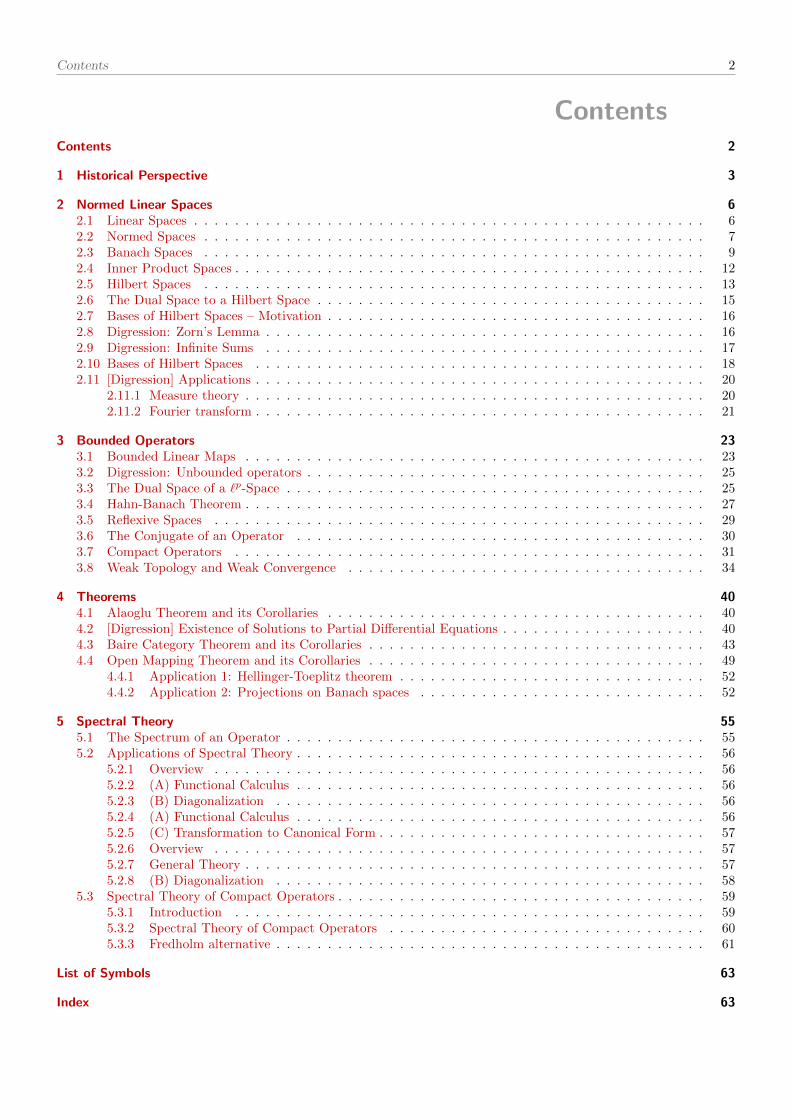
Contents 2
ContentsContents 2
1 Historical Perspective 3
2 Normed Linear Spaces 62.1 Linear Spaces . . . . . . . . . . . . . . . . . . . . . . . . . . . . . . . . . . . . . . . . . . . . . . . . . . 62.2 Normed Spaces . . . . . . . . . . . . . . . . . . . . . . . . . . . . . . . . . . . . . . . . . . . . . . . . . 72.3 Banach Spaces . . . . . . . . . . . . . . . . . . . . . . . . . . . . . . . . . . . . . . . . . . . . . . . . . 92.4 Inner Product Spaces . . . . . . . . . . . . . . . . . . . . . . . . . . . . . . . . . . . . . . . . . . . . . . 122.5 Hilbert Spaces . . . . . . . . . . . . . . . . . . . . . . . . . . . . . . . . . . . . . . . . . . . . . . . . . 132.6 The Dual Space to a Hilbert Space . . . . . . . . . . . . . . . . . . . . . . . . . . . . . . . . . . . . . . 152.7 Bases of Hilbert Spaces – Motivation . . . . . . . . . . . . . . . . . . . . . . . . . . . . . . . . . . . . . 162.8 Digression: Zorn’s Lemma . . . . . . . . . . . . . . . . . . . . . . . . . . . . . . . . . . . . . . . . . . . 162.9 Digression: Infinite Sums . . . . . . . . . . . . . . . . . . . . . . . . . . . . . . . . . . . . . . . . . . . 172.10 Bases of Hilbert Spaces . . . . . . . . . . . . . . . . . . . . . . . . . . . . . . . . . . . . . . . . . . . . 182.11 [Digression] Applications . . . . . . . . . . . . . . . . . . . . . . . . . . . . . . . . . . . . . . . . . . . . 20
2.11.1 Measure theory . . . . . . . . . . . . . . . . . . . . . . . . . . . . . . . . . . . . . . . . . . . . . 202.11.2 Fourier transform . . . . . . . . . . . . . . . . . . . . . . . . . . . . . . . . . . . . . . . . . . . . 21
3 Bounded Operators 233.1 Bounded Linear Maps . . . . . . . . . . . . . . . . . . . . . . . . . . . . . . . . . . . . . . . . . . . . . 233.2 Digression: Unbounded operators . . . . . . . . . . . . . . . . . . . . . . . . . . . . . . . . . . . . . . . 253.3 The Dual Space of a `p-Space . . . . . . . . . . . . . . . . . . . . . . . . . . . . . . . . . . . . . . . . . 253.4 Hahn-Banach Theorem . . . . . . . . . . . . . . . . . . . . . . . . . . . . . . . . . . . . . . . . . . . . . 273.5 Reflexive Spaces . . . . . . . . . . . . . . . . . . . . . . . . . . . . . . . . . . . . . . . . . . . . . . . . 293.6 The Conjugate of an Operator . . . . . . . . . . . . . . . . . . . . . . . . . . . . . . . . . . . . . . . . 303.7 Compact Operators . . . . . . . . . . . . . . . . . . . . . . . . . . . . . . . . . . . . . . . . . . . . . . 313.8 Weak Topology and Weak Convergence . . . . . . . . . . . . . . . . . . . . . . . . . . . . . . . . . . . 34
4 Theorems 404.1 Alaoglu Theorem and its Corollaries . . . . . . . . . . . . . . . . . . . . . . . . . . . . . . . . . . . . . 404.2 [Digression] Existence of Solutions to Partial Differential Equations . . . . . . . . . . . . . . . . . . . . 404.3 Baire Category Theorem and its Corollaries . . . . . . . . . . . . . . . . . . . . . . . . . . . . . . . . . 434.4 Open Mapping Theorem and its Corollaries . . . . . . . . . . . . . . . . . . . . . . . . . . . . . . . . . 49
4.4.1 Application 1: Hellinger-Toeplitz theorem . . . . . . . . . . . . . . . . . . . . . . . . . . . . . . 524.4.2 Application 2: Projections on Banach spaces . . . . . . . . . . . . . . . . . . . . . . . . . . . . 52
5 Spectral Theory 555.1 The Spectrum of an Operator . . . . . . . . . . . . . . . . . . . . . . . . . . . . . . . . . . . . . . . . . 555.2 Applications of Spectral Theory . . . . . . . . . . . . . . . . . . . . . . . . . . . . . . . . . . . . . . . . 56
5.2.1 Overview . . . . . . . . . . . . . . . . . . . . . . . . . . . . . . . . . . . . . . . . . . . . . . . . 565.2.2 (A) Functional Calculus . . . . . . . . . . . . . . . . . . . . . . . . . . . . . . . . . . . . . . . . 565.2.3 (B) Diagonalization . . . . . . . . . . . . . . . . . . . . . . . . . . . . . . . . . . . . . . . . . . 565.2.4 (A) Functional Calculus . . . . . . . . . . . . . . . . . . . . . . . . . . . . . . . . . . . . . . . . 565.2.5 (C) Transformation to Canonical Form . . . . . . . . . . . . . . . . . . . . . . . . . . . . . . . . 575.2.6 Overview . . . . . . . . . . . . . . . . . . . . . . . . . . . . . . . . . . . . . . . . . . . . . . . . 575.2.7 General Theory . . . . . . . . . . . . . . . . . . . . . . . . . . . . . . . . . . . . . . . . . . . . . 575.2.8 (B) Diagonalization . . . . . . . . . . . . . . . . . . . . . . . . . . . . . . . . . . . . . . . . . . 58
5.3 Spectral Theory of Compact Operators . . . . . . . . . . . . . . . . . . . . . . . . . . . . . . . . . . . . 595.3.1 Introduction . . . . . . . . . . . . . . . . . . . . . . . . . . . . . . . . . . . . . . . . . . . . . . 595.3.2 Spectral Theory of Compact Operators . . . . . . . . . . . . . . . . . . . . . . . . . . . . . . . 605.3.3 Fredholm alternative . . . . . . . . . . . . . . . . . . . . . . . . . . . . . . . . . . . . . . . . . . 61
List of Symbols 63
Index 63
1 Historical Perspective 3
HistoricalPerspective 1
2015-0
4-1
4
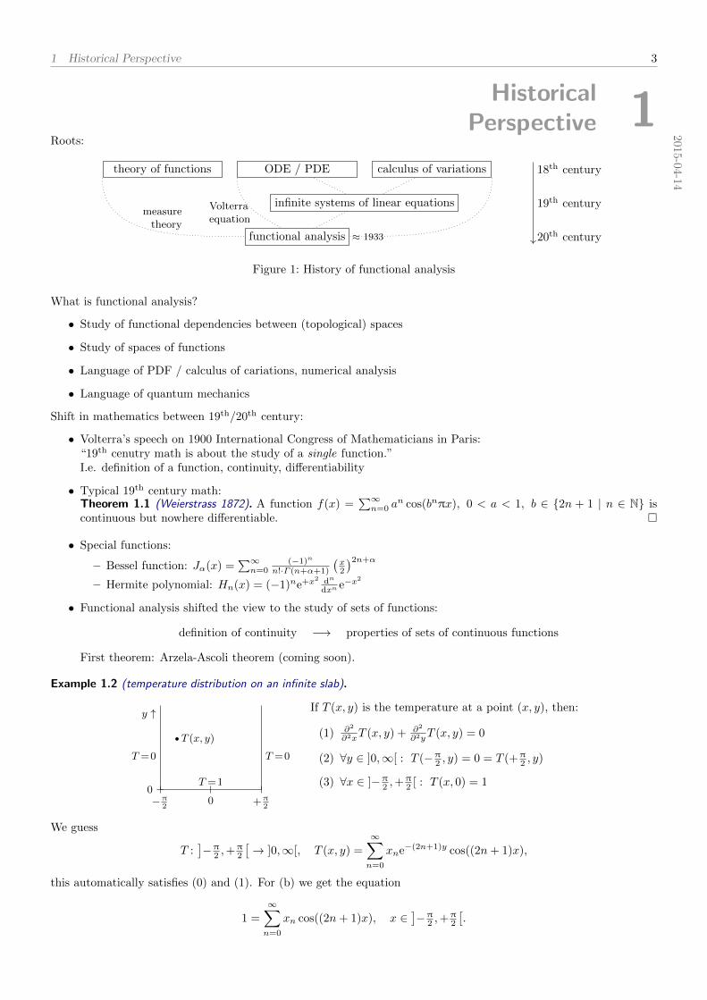
Roots:
theory of functions ODE / PDE calculus of variations
infinite systems of linear equations
functional analysis ≈ 1933
measuretheory
Volterraequation
18th century
19th century
20th century
Figure 1: History of functional analysis
What is functional analysis?
• Study of functional dependencies between (topological) spaces
• Study of spaces of functions
• Language of PDF / calculus of cariations, numerical analysis
• Language of quantum mechanics
Shift in mathematics between 19th/20th century:
• Volterra’s speech on 1900 International Congress of Mathematicians in Paris:“19th cenutry math is about the study of a single function.”I.e. definition of a function, continuity, differentiability
• Typical 19th century math:Theorem 1.1 (Weierstrass 1872). A function f(x) =
∑∞n=0 a
n cos(bnπx), 0 < a < 1, b ∈ 2n + 1 | n ∈ N iscontinuous but nowhere differentiable.
• Special functions:
– Bessel function: Jα(x) =∑∞n=0
(−1)n
n!·Γ (n+α+1)
(x2
)2n+α
– Hermite polynomial: Hn(x) = (−1)ne+x2 dn
dxn e−x2
• Functional analysis shifted the view to the study of sets of functions:
definition of continuity −→ properties of sets of continuous functions
First theorem: Arzela-Ascoli theorem (coming soon).
Example 1.2 (temperature distribution on an infinite slab).
y ↑
00−π
2+π
2
T (x, y)
T =1
T =0 T =0
If T (x, y) is the temperature at a point (x, y), then:
(1) ∂2
∂2xT (x, y) + ∂2
∂2yT (x, y) = 0
(2) ∀y ∈ ]0,∞[ : T (−π2 , y) = 0 = T (+π
2 , y)
(3) ∀x ∈ ]−π2 ,+
π2 [ : T (x, 0) = 1
We guess
T :]−π
2 ,+π2
[→ ]0,∞[, T (x, y) =
∞∑n=0
xne−(2n+1)y cos((2n+ 1)x),
this automatically satisfies (0) and (1). For (b) we get the equation
1 =
∞∑n=0
xn cos((2n+ 1)x), x ∈]−π
2 ,+π2
[.

1 Historical Perspective 4
By subsequent differentiating and putting x = 0 we get:
1 = x0 + 30x1 + 70x2 + . . .
0 = x0 + 32x1 + 72x2 + . . .
0 = x0 + 34x1 + 74x2 + . . . ♦
We got a set of equations of the form:
∞∑n=1
anmxm = yn i.e.
a11 a12 · · ·a21 a22
.... . .
·x1
x2
...
=
y1
y2
...
(∗)
Problem:∞∑n=1
anmxm = yn, anm, yn ∈ F (= R or C) given, xm unknown
How to solve it: 19th century: finite approximations:
pick N : N -th approximation
N∑n=1
anmx(N)m = yn, n = 1, . . . , N =⇒ get x(N)
mtake−−−−→n→∞
xm
Example 1.3.
Consider the following system:
x1 + x2 + . . . = 1
x2 + x3 + . . . = 1
x3 + x4 + . . . = 1
Then:
for odd N : x(N) = (1, 0, 1, 0, . . . )
for even N : x(N) = (0, 1, 0, 1, . . . )
By looking: x = ( 12 ,
12 ,
12 ,
12 , . . . ). ♦
Options one can encounter:
(A) x(N) does converge, and the limit is a solution of eq. (∗)
(B) x(N) does not converge, but eq. (∗) has a solution
(C) x(N) does not converge, and eq. (∗) has no solution
(D) x(N) does converge, but eq. (∗) has no solution
Question: What is the problem we are facing?
2015-04-17
Recall that we studied equations∞∑m=1
anmxm = yn ! Ax = y.
Here is one more example that leads to such an equation:
Example 1.4 (Volterra equation). Let K : [0, 1] × [0, 1] → R and g : [0, 1] → R be continuous functions. The Volterraequation is:
Volterra equation of 1st kind:
∫ s
0
K(s, t) · f(t) dt = g(s)
Volterra equation of 2nd kind: f(s)−∫ s
0
K(s, t) · f(t) dt = g(s)
Riemann integration: Divide [0, 1] into N subintervals, t(N)n = n
N , n = 0, . . . , N :
∫ t(N)n
0
K(t(N)n , t) f(t) dt =
N∑m=1
K(t(N)n , t(N)
m ) f(tN)m ) 1
N + o( 1N )

1 Historical Perspective 5
Volterra equation of 1st kind:
a(N)11 x
(N)1 + a
(N)12 x
(N)2 + · · · + a
(N)1N x
(N)N = y
(N)1
a(N)21 x
(N)1 + a
(N)22 x
(N)2 + · · · + a
(N)2N x
(N)N = y
(N)2
......
......
a(N)N1 x
(N)1 + a
(N)N2 x
(N)2 + · · · + a
(N)NNx
(N)N = y
(N)N
a(N)nm = K(t(N)
n , t(N)m ) 1
N
x(N)m = f(t(N)
m )
y(N)n = g(t(N)
n )
Now:∞∑m=1
a(N)nm x
(N)m = y(N)
n , x(N)btNc
N→∞−→ f(t), t ∈ ]0, 1[ ♦
Historical perspective – overview:
(1)∑∞m=1 anmxm = yn is linear Ax = y where x! (xn)∞n=1
(2) ∂2
∂x2u(x, y) + ∂2
∂y2u(x, y) = 0 is linear Ax = y where x! u(x, y)
(3)∫ s
0K(s, t) f(t) dt = g(s) is linear Ax = y where x! f(t)
Problems:
(1) Notion of solution
(2) Continuity with respect to data
Concerning the continuity with respect to data:
Prop. 1.5. Let A(t) = (aij(t))ni,j=1 be a matrix that depends smoothly on t (smooth family), and vectors y(t) =
(yj(t))nj=1 smoothly on t. Suppose in addition ∀t : kerA(t) = 0. Then the solution x(t) of A(t)x(t) = y(t) depends
smoothly on t.
Proof. Observe detA is a smooth function:
detA =∑π
(−1)sgnπa1,π(1)a2,π(2) . . . an,π(n), xj =det ‖ · ‖detA(t)
∴ detA is a smooth function
Chapters:
• Normed linear spaces, Banach spaces, Hilbert spaces
• Linear operators on Banach spaces, dual spaces
• little bit more topology
• Three big results in functional analysis: Hahn-Banach theorem, Banach-Steinhaus theorem, open mappingprinciple
• Geometry of Banach space
• Compact operators and spectrum
Furthermore, let in the following be F = R or F = C.

2 Normed Linear Spaces 6
Normed LinearSpaces 2
2.1 Linear Spaces
2015-0
4-1
7
Definition 2.1 (linear space). Set X equipped with two operations, on which two operations
addition X ×X → X, (x, y) 7→ x+ y
multiplication by scalar F×X → X, (λ, x) 7→ λ · x
is called linear space over field F, provided the following axioms are satisfied for any x, y, z ∈ X and a, b ∈ F:
Group structure:
• associativity: (x+ y) + z = x+ (y + z)
• identity element: x+ 0 = x
• existence of inverses: x+ (−x) = 0
• commutativity: x+ y = y + x
Compatibility with field:
• compatibility of mul.: a · (b · x) = (ab) · x• compatibility of one: 1 · x = x
• distributivity I: a · (x+ y) = a · x+ a · y• distributivity II: (a+ b) · x = a · x+ b · x
Example 2.2 (examples of linear spaces).
(1) Finite-dimensional euclidean space Rn or Cn
(2) Space of inifinite sequences (xn)∞n=1, xn ∈ F
(3) `p, p =∞, the space of all (xn)∞n=1 with supn∈N|xn| <∞, i.e. the space of all bounded sequences
(4) `p, p ∈ [1,∞[, the space of all (xn)∞n=1 with∑n∈N|xn|p <∞
(5) `p, p ∈ [0, 1[, the space of all (xn)∞n=1 with∑n∈N|xn|p <∞
(6) Space C([0, 1]) of continuous functions on the interval [0, 1]
(7) Solutions of Volterra’s equation
(8) Space of polynomials p ∈ X if ∃n ∈ N : p(x) =∑nj=0 ajx
j ♦
Proof that (4) in example 2.2 is a linear space.If (xn)n with
∑n|xn|p <∞ and (yn)n with
∑n|yn|p <∞, then
∑n|xn + yn|p <∞?
|xn + yn|p ≤ |2xn|p + |2yn|p ≤ 2p(|xn|p + |yn|p).
Remark 2.3 (unit balls in `p). Further investigations of `p-spaces: normable?
x1
x2
unit ball for p =∞
x1
x2
unit ball for p = 2
x1
x2
unit ball for p = 1
x1
x2
unit ball for p = 1/2
Figure 2: Unit balls in `p for some p ∈ [0,∞]//

2 Normed Linear Spaces 7
Definition 2.4 (linear subspace). U ⊆ X is called linear subspace if ∀x1, x2 ∈ U, λ1, λ2 ∈ F : λ1x1 + λ2x2 ∈ U .
Definition 2.5 (sum of subsets in vector spaces). If S, T ⊆ X then S + T := z ∈ X | z = x+ y, x ∈ S, y ∈ T.
Theorem 2.6 (properties of linear subspaces).
(1) 0 and X are linear subspaces.
(2) The intersection of any collection of subspaces is a subspace.
(3) The sum of any collection of subspaces a subspace.
Definition 2.7 (linear span). Given set M ⊆ X, the linear span span(M) is the intersection of all linear subspaces Ysuch that M ⊆ Y .
Theorem 2.8 (properties of the linear span).
(1) The linear span of M is the smallest linear subspace that includes M .
(2) span(M) consists precisely of the vectors∑nj=1 λjxj , n ∈ N, xj ∈M,λj ∈ F.
Definition 2.9 (convex set). Only for F = R! K is convex set if for x1, x2 ∈ K and λ1, λ2 ∈ F, λ1 + λ2 = 1 we haveλ1x1 + λ2x2 ∈ X.
2.2 Normed Spaces
2015-0
4-2
1
Definition 2.10 (normed space). Let X be a linear space and ‖·‖ : X → R a map that satisfies:
(1) non-negativity: ∀x ∈ X : ‖x‖ ≥ 0
(2) absolute homogenity: ∀x ∈ X,λ ∈ F : ‖λ · x‖ = |λ| · ‖x‖(3) triangle inequality: ∀x, y ∈ X : ‖x+ y‖ ≤ ‖x‖ + ‖y‖(4) zero norm ⇒ zero vector: ∀x ∈ X : ‖x‖ = 0 ⇔ x = 0
Then ‖·‖ is called a norm on X, and (X, ‖·‖) is called a normed space. On every normed space, we define a distancefunction d by:
d : X ×X → R, d(x, y) = ‖x− y‖.
Prop. 2.11 (norms are Lipshitz continuous). A norm ‖·‖ : X → R is uniformly continuous, and in fact even Lipshitzcontinuous.
Proof. We have |‖x‖ − ‖y‖| ≤ ‖x− y‖. Put y = −x+ z into (3) to get |‖z‖ − ‖x‖| ≤ ‖z − x‖.
Definition 2.12 (equivalence of norms). Let ‖·‖1 and ‖·‖2 be norms on a vector space X. They are called equivalent if
∃C > 0 : C−1 · ‖·‖2 ≤ ‖·‖1 ≤ C+1 · ‖·‖2,
or equivalent to this condition,∃C,C ′ > 0 : C ′ · ‖·‖2 ≤ ‖·‖1 ≤ C · ‖·‖2.
Theorem 2.13 (equivalence of norms). Norms ‖·‖1 and ‖·‖2 are equivalent iff the topologies they generate are thesame.
Proof.
Proof of “⇒”: Let T1, T2 be topologies. If U ∈ T1. B(1)r := x | ‖x‖1 < r. Then B
(2)C−1δ ⊆
B(1)δ ⊆ B(2)
Cδ .
Proof of “⇐”: B(2)1 ∈ T2 if T1 = T2 therefore B
(1)C ⊇ B(2)
1 . Let x ∈ X. Then x‖x‖2
∈ B(2)1 . With
B(1)C ⊇ B(2)
1 it follows that ‖ x‖x‖2‖1 ≤ C, and hence ‖x‖1 ≤ C‖x‖2.
xB
(2)
C−1δ
B(1)δ
U

2 Normed Linear Spaces 8
Theorem 2.14 (norms in finite-dim are equivalent). All norms on a finite dimensional space are equivalent.
Proof.
The one inequality. Let e1, . . . , en be a basis of X, so for any x ∈ X we have x = x1e1 + . . . + xne
n. Consider theinfinity-norm ‖x‖∞ = max1≤j≤n|xj |. Let ‖·‖ be a different norm. Then
‖x‖ =∥∥x1e
1 + . . .+ xnen∥∥
≤ |x1|∥∥e1∥∥ + . . .+ |xn|‖en‖
≤ ‖x‖∞ ·(∥∥e1
∥∥ + . . .+ ‖en‖)︸ ︷︷ ︸
=:C
.
The other inequality. We observe that ‖·‖ is continuous in T∞ (because ‖x‖ ≤ C · ‖x‖∞). Let S∞1 := x | ‖x‖∞ = 1,then S∞1 is compact, and hence a minimum exists, minx∈S∞1 ‖x‖ =: δ > 0 (where the latter inequality follows from0 /∈ S∞1 ). For any x ∈ X we have x
‖x‖∞∈ S∞1 , whereat∥∥∥∥ x
‖x‖∞
∥∥∥∥ ≥ δ ∴ ‖x‖ ≥ δ‖x‖∞.
Theorem 2.15 (compactness of the closed unit ball). Closed unit ball B1 := x ∈ X | ‖x‖ ≤ 1 is compact iff dimensionof X is finite.
Proof of theorem 2.15 – part 1/2. If X is infinite-dimensional, then B1 is not compact.
Example 2.16. (`∞, ‖·‖∞), i.e. all bounded sequences, where ‖x‖∞ = supj∈N|xj |. Then ∀j : ‖ej‖∞ = 1 and ∀j 6= k :
‖ej − ek‖∞ = 1, where
e1 = (1, 0, 0, 0, . . . )
e2 = (0, 1, 0, 0, . . . )
e3 = (0, 0, 1, 0, . . . ).
In particular e1, e2, e3, . . . is neither convergent nor Cauchy. ♦
Lemma 2.17 (existence of projections). Let U be a proper closed linear subspace of X. Then there exists x /∈ U with‖x‖ = 1 such that dist(x, U) ≥ 1
2 , where dist(x, U) = infy∈U‖x− y‖.
Proof.Pick any x /∈ U , then dist(x, U) = d > 0 (because U is closed). Pick y0 ∈ U such that‖x − y0‖ = 2d. Claim ist that x := x−y0
2d satisfies the requirements. Clearly ‖x‖ = 1. Lety ∈ U . Then U
z z
y0
‖x− y‖ =
∥∥∥∥ x− y0
2d− y∥∥∥∥ =
∥∥∥∥ x− y0 − 2dy
2d
∥∥∥∥ ≥ d
2d=
1
2.
Since U is linear subspace y0 + 2dy ∈ U , and hence‖x−z‖2d≥
d2d = 1
2 .
Remark 2.18.
Concering the dist(x, U) = infy∈U‖x− y‖: There exists a sequence yn ∈ U such that‖yn−x‖
n→∞−→ d, in particular for any ε > 0 there is a y(ε) such that ‖y(ε)−x‖ ≤ d+ε.If instead of y(ε) you consider λy(ε), εR.
F (λ) := ‖λy(ε)− x‖, λ ∈ R U
1y0
x
d+ ε2d
//
Proof of theorem 2.15 – part 2/2. If X is infinite-dimensional, then Bn is not compact. We construct a sequence(x0, x1, . . . , xn, . . . ), xj ∈ X where x0 is arbitrary with ‖x0‖ = 1. Given (x0, . . . , xn) then consider spanx1, . . . , xn =:U (closed because of finite dimensional, and hence proper). Use the lemma to pick xn+1 such that ∀j : ‖xj‖ = 1 and∀j 6= k : ‖xj − xk‖ ≥ 1
2 .
2 Normed Linear Spaces 9
Remark 2.19. We have a look at subspaces of (c, ‖·‖):
‖x‖ = maxn∈N|xn|
c0 =
infinite real sequences (xn)n∈N
∣∣∣ limn→∞
xn = 0
ccpt = sequences (xn)n∈N | (xn)n∈N has only finitely many non-zero elementsccpt is a proper subspace of c //
2015-0
4-2
4
Repitition:– equivalent norms– topologies– finite-dimensional ⇔ all norms equivalent– unit ball is not compact in infinite-dimensional spaces
Question: Suppose you have two topologies T1, T2 induces by norms ‖·‖1, ‖·‖2. . . .
2.3 Banach Spaces
Definition 2.20 (Banach space). Banach space is a normed linear space that is complete.
Motivation: Why Banach?– numerical analysis: limn→∞ xn, |xn − xk| < precision, n, k ≥ n0
– pure math: xn+1 = F (xn, xn−1), limn→∞ xn = x ⇔ x = F (x, x)
Example 2.21 (examples and counterexamples for banach spaces).
(1) c, the space of real/complex sequences (xn)∞n=1 such that limn→∞ xn exists. Equipped with norm ‖(xn)n‖ =maxn∈N|xn| it is Banach.
(2) c0, the space c0 ⊆ c of sequences such that limn→∞ xn = 0. This is a closed subspace, hence a Banach space.
(3) ccpt, the space ccpt ⊆ c0 of sequences with finite number of non-zero elements.Claim. ccpt is a proper dense subspace of c0.Proof.Proper: xn = 1
n .
Dense: Let (xn)n ∈ c0 and pick ε. Find N such that |xn| ≤ ε for n ≥ N . Define x(N)n =
xn for n≤N0 for n>N . Clearly
(x(N)n )n ∈ ccpt. Furthermore ‖(x(N)
n )n − (xn)n‖ = maxn|x(N)n − xn| = maxn≥N |xn| ≤ ε.
(4) Let (M,d) be a metric space and K ⊆M be a compact set.C(K), the space of all continuous functions f : K → R.Norm on this space: ‖f‖∞ = supx∈K |f(x)| (called the max-norm or sup-norm) ♦
Concering the fourth example:Question: If fn ∈ C(K) such that ∀x ∈ K : limn→∞ fn(x) = f(x), does it imply that f ∈ C(K)?Negative answer: No!, take fn = xn.Positive answer: Yes!, if fn ⇒ f . Recall:
fn → f ⇔ ∀x : ∀ε > 0 ∃n0 ∈ N ∀n ≥ n0 : |fn(x)− f(x)| ≤ εfn ⇒ f ⇔ ∀ε > 0 ∃n0 ∈ N ∀n ≥ n0 : ∀x : |fn(x)− f(x)| ≤ ε
⇔ ∀ε > 0 ∃n0 ∈ N ∀n ≥ n0 : maxx∈K |fn(x)− f(x)| ≤ ε⇔ ∀ε > 0 ∃n0 ∈ N ∀n ≥ n0 : ‖fn − f‖∞ ≤ ε⇔ ‖fn − f‖∞
n→∞−→ 0.
Remark 2.22 (convergence in sup-Norm = uniform convergence). Notion if convergence w.r.t. the norm ‖·‖∞ is equiv-alent to the notation of uniform convergence. //
2 Normed Linear Spaces 10
Theorem 2.23 ((C(K), ‖·‖∞) is complete). (C(K), ‖·‖∞) is a Banach space.
Proof. If fn ∈ C(K) Cauchy sequence, ‖fn − fk‖∞ = maxx∈K |fn(x) − fk(x)| ≤ ε if n, k ≥ N , then fn −→ f . Foreach x ∈ K, then fn(x) is a Cauchy sequence, then f(x) := limn→∞ fn(x) exists.To show:
(a) ‖fn − f‖∞ −→ 0(b) f ∈ C(K)
Proof:(a) Pick N from above. Then
‖f − fN‖∞ = maxx∈K|f(x)− fN (x)|
= maxx∈K
limn→∞
|fn(x)− fN (x)|
≤ supx∈K
supn≥N|fn(x)− fN (x)|
≤ supn≥N
supx∈K|fn(x)− fN (x)|
≤ ε.
(b) Fix N such that |f(x) − fN (x)| ≤ ε3 and |f(y) − fN (y)| ≤ ε
3 . Now since fN continuous choose x, y such that|fN (x)− fN (y)| < ε
3 if d(x, y) < δ. Then
|f(x)− f(y)| ≤ |f(x)− fN (x)|︸ ︷︷ ︸≤ε/3
+ |fN (x)− fN (y)|︸ ︷︷ ︸≤ε/3
+ |f(y)− fN (y)|︸ ︷︷ ︸≤ε/3
≤ ε.
What are compact subsets of C(K)?
Prop. 2.24 (characterization of relative compactness). The following is equivalent for subsets N of complete metricspaces:
(i) N compact
(ii) Every sequence (xn)n∈N, xn ∈ N has a convergent subsequence
(iii) For each ε > 0 exists a finite number of xj ∈ N, j = 1, . . . , n such that⋃j=1,...,nBε(xj) = N
Remark 2.25 (prequesits for Arzela-Ascoli). Let K be a compact set, and consider (C(K), ‖·‖∞), and let F ⊆ C(K).
Recall that:– F is bounded if supf∈F‖f‖∞ <∞.– F is called equicontinuous if
∀x : ∀ε > 0 ∃δ > 0 ∀f ∈ F : ∀y : d(x, y) ≤ δ ⇒ |f(x)− f(y)| ≤ ε.//
2015-04-28
Repitition:– (relative) compactness– Arzela-Ascoli theorem– equicontinuity
Prop. 2.26 (continuous functions map compact sets to compact sets). Continuous functions map compact sets tocompact sets. In particular, continuous function on a compact set attains its maxima/minima.
Motivation: Problem: Given function f : K → R, find minx∈K f(x). → find a topology, that has so much open setssuch that f is continuous, but so less open sets, such that K is compact.
Remark 2.27. Every finite set of continuous functions is equicontinuous. //
Theorem 2.28 (Arzela-Ascoli). Let K be a compact set, and consider (C(K), ‖·‖∞), and let F ⊆ C(K). Then F isrelatively compact, iff F is equicontinuous and bounded.
2 Normed Linear Spaces 11
Proof of F relatively compact ⇒ F equicontinuous & bounded.
For any ε there are functions fjN(ε)j=1 such that:⋃N(ε)
j=1 Bε(fj) ⊇ F .
Let f ∈ F and pick x, then
|f(x)− f(y)| ≤ |f(x)− fj(x)| + |f(y)− fj(y)| + |fj(x)− fj(y)| ≤ 3ε,
where pick a j such that ‖f − fj‖ ≤ ε, and a δ such that d(x, y) ≤ δ ⇒ |fj(x)− fj(y)| ≤ ε.
Kfj
fx
Idea for bounded is similar.
Proof of F relatively compact ⇐ F equicontinuous & bounded.
We need to prove that given fn ∈ F , then there is a subsequence fn(j) such that limj→∞ fn(j)
exists.
• ∃f ∈ C(K) : ‖f − fn(j)‖ −→ 0
• For j, k large ‖fn(k) − fn(j)‖ −→ 0 meaning that subsequence fn(j) is cauchy.
K
z Kε(z)
Steps (overview):
1. Find the covering K ⊆⋃z∈S Kr(z), i.e. construct such Kr(z)’s and S.
2. Diagonal trick:Consider fn(z) for z ∈ S. Then there is a n(j) such that fn(j)(z) converges for all z ∈ S (use boundness).
3. Use construction of S to prove that fn(j)(z) is Cauchy (use equicontinuity).
Steps (details):
1. Construction of Kε(z)’s:For each ε > 0 and z ∈ K define
Kε(z) = x ∈ K | ∀f ∈ F|f(z)− f(x)| ≤ ε.
Because F is equicontinuous, Kε(z) is nonempty and open, and K ⊆⋃z∈K Kε(z).
Construction of S:Pick N such that K ⊆
⋃z∈K K1/N (z). Choose KN ⊆ K such that KN = z1, . . . , zn discrete set and
K ⊆⋃z∈K
K1/N (z) ⊆⋃
z∈KN
K1/N (z).
Define S :=⋃N∈NKN , then S is countable.
3. Claim: fn(j) constructed in step 2 is a Cauchy sequence.Proof: For all x ∈ K and z ∈ S it holds that∣∣fn(j)(x)− fn(k)(x)
∣∣ ≤ ∣∣fn(j)(x)− fn(j)(z)∣∣ +
∣∣fn(k)(x)− fn(k)(z)∣∣ +
∣∣fn(j)(z)− fn(k)(z)∣∣.
Pick N > 0 and z ∈ KN such that |fn(j)(x)−fn(j)(z)| ≤ 1N for all j. Pick j, k such that |fn(j)(z)−fn(k)(z)| ≤ 1
N .Then for all x there exists N,n0 such that
j, k ≥ n0 ⇒∣∣fn(j)(x)− fn(k)(x)
∣∣ ≤ 3N ,
and hence ‖fn(j) − fn(k)‖ ≤ 3N .
2. Lemma (diagonal trick). Let S be a countable set and let fn(z), n ∈ N be a sequence such that there is a M > 0with ∀n ∈ N, z ∈ S : |fn(z)| ≤ M . Then there exists a subsequence n(j) such that fn(j)(z) is convergent for allz ∈ S.Proof. Since S is countable, S = z1, z2, . . . = zmm∈N. Then we have sequencesfn(zm). Because the sequence fn(z1)n∈N is bounded, there is a subsequence n1(j)such that fn1(j)(z1) is convergent, and there is a subsequence n2(j) of n1(j) such thatfn2(j)(z2) is convergent, and so on. Continuing this process, you can find subsequencenm(j) such that fnm(j)(zk) converges for k ≤ m.Naive: Define n∞(j) := limm→∞ nm(j). It may happen that limm→∞ nm(1) =∞.Correct: Pick a subsequence n∞(j) := nj(j). Claim is that fnj(j)(z) is convergent forall z ∈ S.Proof: Pick any z, let say z = z100, then fnj(j) is convergent, n100(j) is a subsequencefor which fn100(j)(z100) is convergent.
n
m
f1(z1) f2(z1) · · ·f1(z2)
· · ·
2 Normed Linear Spaces 12
This finishes the proof.
2.4 Inner Product Spaces
2015-0
5-0
5
Definition 2.29 (inner product space). Let V be a linear space and 〈·, ·〉 : V × V → C a map that satisfies
(1) non-negativity: ∀x ∈ V : 〈x, x〉 ≥ 0
(2) linear in 2nd argument: ∀x, y ∈ V, λ ∈ C : 〈x, αy〉 = α〈x, y〉(3) linear in 2nd argument: ∀x, y, z ∈ V : 〈x, y + z〉 = 〈x, y〉 + 〈x, z〉(4) hermitian: ∀x, y ∈ V : 〈x, y〉 = 〈y, x〉(5) definiteness: ∀x ∈ V : 〈x, x〉 = 0⇔ x = 0
Then 〈·, ·〉 is called a scalar product in V , and (V, 〈·, ·〉) is called a normed space. We claim:
(2’) semilinear in 1st argument: ∀x, y ∈ V, λ ∈ C : 〈αx, y〉 = α〈x, y〉(3’) semilinear in 1st argument: ∀x, y, z ∈ V : 〈x+ y, z〉 = 〈x, z〉 + 〈y, z〉
Furthermore, the scalarproduct 〈·, ·〉 induces a norm ‖·‖ by
‖·‖ : V → R, ‖x‖ :=√〈x, x〉.
Example 2.30 (examples of inner product spaces).
(1) Cn equipped with 〈x, y〉 =∑nj=1 xj · yj is an inner product space, and a Banach space.
(2) C([0, 1]) equipped with 〈f, g〉 =∫ 1
0f(x) · g(x) dx is an inner product space, but not a Banach space. ♦
Definition 2.31 (orthogonality).
Vectors x, y are orthogonal, x ⊥ y, if 〈x, y〉 = 0. A set of vectors xjj∈J is called an orthonormalset, if they are mutually orthogonal and ∀j ∈ J : ‖xj‖ = 1.
The Pythagorean theorem states that, if x ⊥ y then ‖x + y‖2 = ‖x‖2 + ‖y‖2. We generalize thisstatement.
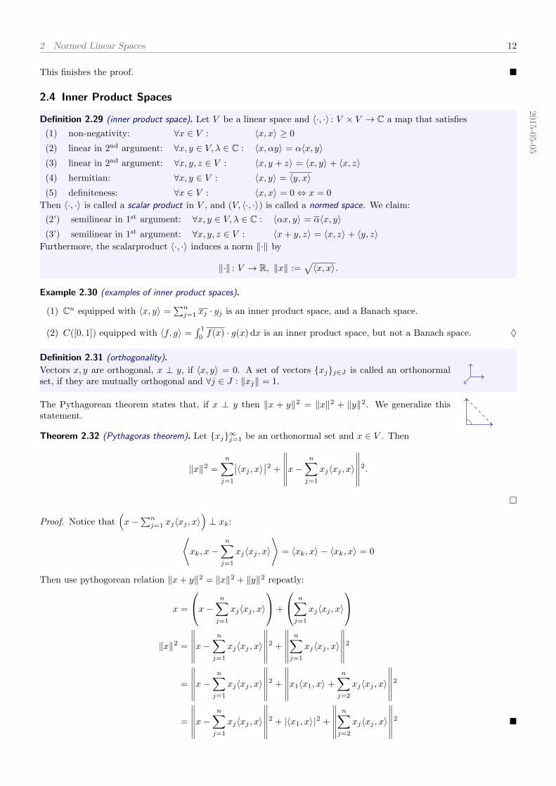
Theorem 2.32 (Pythagoras theorem). Let xj∞j=1 be an orthonormal set and x ∈ V . Then
‖x‖2 =
n∑j=1
∣∣〈xj , x〉∣∣2 +
∥∥∥∥∥∥x−n∑j=1
xj〈xj , x〉
∥∥∥∥∥∥2.
Proof. Notice that(x−
∑nj=1 xj〈xj , x〉
)⊥ xk:⟨
xk, x−n∑j=1
xj〈xj , x〉
⟩= 〈xk, x〉 − 〈xk, x〉 = 0
Then use pythogorean relation ‖x+ y‖2 = ‖x‖2 + ‖y‖2 repeatly:
x =
x− n∑j=1
xj〈xj , x〉
+
n∑j=1
xj〈xj , x〉
‖x‖2 =
∥∥∥∥∥∥x−n∑j=1
xj〈xj , x〉
∥∥∥∥∥∥2 +
∥∥∥∥∥∥n∑j=1
xj〈xj , x〉
∥∥∥∥∥∥2
=
∥∥∥∥∥∥x−n∑j=1
xj〈xj , x〉
∥∥∥∥∥∥2 +
∥∥∥∥∥∥x1〈x1, x〉 +
n∑j=2
xj〈xj , x〉
∥∥∥∥∥∥2
=
∥∥∥∥∥∥x−n∑j=1
xj〈xj , x〉
∥∥∥∥∥∥2 + |〈x1, x〉|2 +
∥∥∥∥∥∥n∑j=2
xj〈xj , x〉
∥∥∥∥∥∥2

2 Normed Linear Spaces 13
Corollary 2.33 (Bessel inequality). For any orthonormal set xjnj=1 and vector x ∈ V , we so-called Bessel inequalityholds, that is
‖x‖2 ≥n∑j=1
∣∣〈xj , x〉∣∣2.
Corollary 2.34 (Cauchy-Schwarz inequality). For all x, y ∈ V it holds that
‖x‖ · ‖y‖ ≥ |〈x, y〉|.
Proof of Cauchy-Schwarz – using Bessel inequality. For any y 6= 0 y‖y‖ is an orthonormal set. Bessel inequality
implies
‖x‖2 ≥∣∣∣∣⟨ y
‖y‖, x
⟩∣∣∣∣2 =|〈x, y〉|2
‖y‖2.
Proof of Cauchy-Schwartz – typical proof. Suppose 〈x, y〉 ∈ R. Then for all t ∈ R we have that
0 ≤ 〈x− ty, x− ty〉 = ‖x‖2 − 2t〈x, y〉 + t2‖y‖2.
This expression is minimal at t =〈x,y〉‖y‖2 , and so
0 ≤ ‖x‖2 −|〈x, y〉|2
‖y‖2.
Every parallelogram, e.g. the one drawn on the righthand side, satisfies the identity
|AB|2 + |BC|2 + |CD|2 + |DA|2 = |AC|2 + |BD|2.
We transfer this identity to normed spaces (where it doesn’t have to be true, cf. proposi-tion 2.35), and call it parallelogram identity :
∀x, y ∈ V : ‖x+ y‖2 + ‖x− y‖2 = 2(‖x‖2 + ‖y‖2
).
A
B
C
D
Prop. 2.35 (characterization of inner product spaces). Norm is associated to a scalar product, iff the parallelogramidentity holds.
2.5 Hilbert Spaces
Definition 2.36 (Hilbert space). An inner product space complete in this norm is called a Hilbert space.
Example 2.37 (examples of Hilbert spaces).
(3) L2([0, 1]) of functions with∫ 1
0|f(x)|2 dx < 0, equipped with 〈f, g〉 :=
∫ 1
0f(x) · g(x) dx is a Hilbert space.
(4) `2 of sequences with∑∞n=1|xn|2 <∞, equipped with 〈x, y〉 :=
∑∞n=1 xn · yn is a Hilbert space. ♦
Remark 2.38. No other `p spaces, except for `2, are Hilbert spaces. //
Prop. 2.39 (product of Hilbert spaces). Let H1,H2 be two Hilbert spaces. Then H1 ×H2 := (x, y) | x ∈ H1, y ∈ H2is a Hilbert space with inner product 〈(x1, y1), (x2, y2)〉 = 〈x1, x2〉H1
+ 〈y1, y2〉H2.
Remark 2.40. Preview: Decomposition of Hilbert spaces: “R2 = Rx × Ry”. xy
//
Definition 2.41 (orthogonal complement). Let U be a linear subspace of H. Then U⊥ := x ∈ H | ∀y ∈ U : x ⊥ y
Lemma 2.42 (properties of the orthogonal complement). U⊥ is linear subspace, and in fact it is a closed subspace.
Proof. Closed: Exercise. Linear: If y1, y2 ∈ U⊥, then also αy1 + βy2 ∈ U⊥. Pick x ∈ U , we need to prove
〈x, αy1 + βy2〉 = α〈x, y1〉 + β〈x, y2〉 = 0.
2 Normed Linear Spaces 14
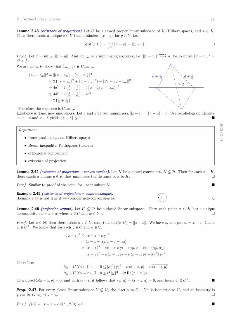
Lemma 2.43 (existence of projections). Let U be a closed proper linear subspace of H (Hilbert space), and x ∈ H.Then there exists a unique z ∈ U that minimizes ‖x− y‖ for y ∈ U , i.e.
dist(x, U) := infy∈U‖x− y‖ = ‖x− z‖.
Proof. Let d := infy∈U‖x− y‖. And let zn be a minimizing sequence, i.e. ‖x− zn‖n→∞−→ d, for example ‖x− zn‖2 =
d2 + 1n .
We are going to show that (zn)n∈N is Cauchy.
‖zn − zm‖2 = ‖(x− zm)− (x− zn)‖2
= 2(‖x− zn‖2 + ‖x− zm‖2
)− ‖2x− zn − zm‖2
= 4d2 + 2(
1n + 1
m
)− 4∥∥x− 1
2 (zn + zm)∥∥2
≤ 4d2 + 2(
1n + 1
m
)− 4d2
= 2(
1n + 1
m
)Therefore the sequence is Cauchy.
x
zm zn
d+ 1m d+ 1
n
≥ d
Existance is done, now uniqueness. Let z and z be two minimizers, ‖x− z‖ = ‖x− z‖ = d. Use parallelogram identityon x− z and x− z yields ‖z − z‖ ≤ 0.
2015-0
5-0
8
Repitition:
• Inner product spaces, Hilbert spaces
• Bessel inequality, Pythogoras theorem
• orthogonal complement
• existence of projection
Lemma 2.44 (existence of projections – convex version). Let K be a closed convex set, K ⊆ H. Then for each x ∈ H,there exists a unique y ∈ K that minimizes the distance of x to K.
Proof. Similar to proof of the same for linear subset K.
Example 2.45 (existence of projections – counterexample).Lemma 2.44 is not true if we consider non-convex spaces. ♦
Lemma 2.46 (projection lemma). Let U ⊆ H be a closed linear subspace. Then each point x ∈ H has a uniquedecompositon x = z + w where z ∈ U and w ∈ U⊥.
Proof. Let x ∈ H, then there exists a z ∈ U , such that dist(x, U) = ‖z − x‖. We have z, and put w = x − z. Claimw ∈ U⊥. We know that for each y ∈ U and α ∈ C:
‖x− z‖2 ≤ ‖x− z − αy‖2
= 〈x− z − αy, x− z − αy〉= ‖x− z‖2 − 〈x− z, αy〉 − 〈αy, x− z〉 + 〈αy, αy〉
= ‖x− z‖2 − α〈x− z, y〉 − α〈x− z, y〉 + |α|2‖y‖2
Therefore:∀y ∈ U ∀α ∈ C : 0 ≤ |α|2‖y‖2 − α〈x− z, y〉 − α〈x− z, y〉∀y ∈ U ∀α = r ∈ R : 0 ≤ t2‖y‖2 − 2tRe〈x− z, y〉
Therefore Re〈x− z, y〉 = 0, and with α = it it follows that 〈w, y〉 = 〈x− z, y〉 = 0, and hence w ∈ U⊥.
Prop. 2.47. For every closed linear subspace U ⊆ H, the dirct sum U ⊕ U⊥ is isometric to H, and an isometry isgiven by (z, w) 7→ z + w.
Proof. f(α) = ‖x− z − αy‖2, f ′(0) = 0.
2 Normed Linear Spaces 15
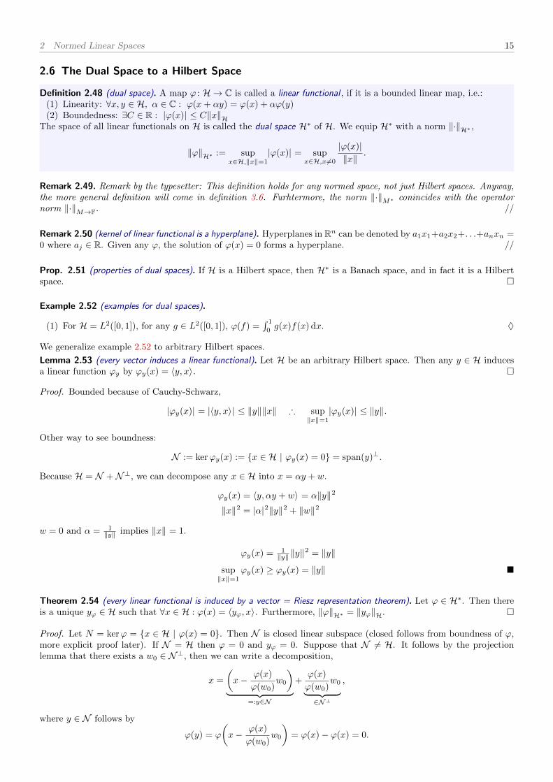
2.6 The Dual Space to a Hilbert Space
Definition 2.48 (dual space). A map ϕ : H → C is called a linear functional , if it is a bounded linear map, i.e.:(1) Linearity: ∀x, y ∈ H, α ∈ C : ϕ(x+ αy) = ϕ(x) + αϕ(y)(2) Boundedness: ∃C ∈ R : |ϕ(x)| ≤ C‖x‖H
The space of all linear functionals on H is called the dual space H∗ of H. We equip H∗ with a norm ‖·‖H∗ ,
‖ϕ‖H∗ := supx∈H,‖x‖=1
|ϕ(x)| = supx∈H,x 6=0
|ϕ(x)|‖x‖
.
Remark 2.49. Remark by the typesetter: This definition holds for any normed space, not just Hilbert spaces. Anyway,the more general definition will come in definition 3.6. Furhtermore, the norm ‖·‖M∗ conincides with the operatornorm ‖·‖M→F. //
Remark 2.50 (kernel of linear functional is a hyperplane). Hyperplanes in Rn can be denoted by a1x1+a2x2+. . .+anxn =0 where aj ∈ R. Given any ϕ, the solution of ϕ(x) = 0 forms a hyperplane. //
Prop. 2.51 (properties of dual spaces). If H is a Hilbert space, then H∗ is a Banach space, and in fact it is a Hilbertspace.
Example 2.52 (examples for dual spaces).
(1) For H = L2([0, 1]), for any g ∈ L2([0, 1]), ϕ(f) =∫ 1
0g(x)f(x) dx. ♦
We generalize example 2.52 to arbitrary Hilbert spaces.
Lemma 2.53 (every vector induces a linear functional). Let H be an arbitrary Hilbert space. Then any y ∈ H inducesa linear function ϕy by ϕy(x) = 〈y, x〉.
Proof. Bounded because of Cauchy-Schwarz,
|ϕy(x)| = |〈y, x〉| ≤ ‖y‖‖x‖ ∴ sup‖x‖=1
|ϕy(x)| ≤ ‖y‖.
Other way to see boundness:
N := kerϕy(x) := x ∈ H | ϕy(x) = 0 = span(y)⊥.
Because H = N +N⊥, we can decompose any x ∈ H into x = αy + w.
ϕy(x) = 〈y, αy + w〉 = α‖y‖2
‖x‖2 = |α|2‖y‖2 + ‖w‖2
w = 0 and α = 1‖y‖ implies ‖x‖ = 1.
ϕy(x) = 1‖y‖ ‖y‖
2 = ‖y‖
sup‖x‖=1
ϕy(x) ≥ ϕy(x) = ‖y‖
Theorem 2.54 (every linear functional is induced by a vector = Riesz representation theorem). Let ϕ ∈ H∗. Then thereis a unique yϕ ∈ H such that ∀x ∈ H : ϕ(x) = 〈yϕ, x〉. Furthermore, ‖ϕ‖H∗ = ‖yϕ‖H.
Proof. Let N = kerϕ = x ∈ H | ϕ(x) = 0. Then N is closed linear subspace (closed follows from boundness of ϕ,more explicit proof later). If N = H then ϕ = 0 and yϕ = 0. Suppose that N 6= H. It follows by the projectionlemma that there exists a w0 ∈ N⊥, then we can write a decomposition,
x =
(x− ϕ(x)
ϕ(w0)w0
)︸ ︷︷ ︸
=:y∈N
+ϕ(x)
ϕ(w0)w0︸ ︷︷ ︸
∈N⊥
,
where y ∈ N follows by
ϕ(y) = ϕ
(x− ϕ(x)
ϕ(w0)w0
)= ϕ(x)− ϕ(x) = 0.

2 Normed Linear Spaces 16
All functionals α〈w0, x〉, α ∈ C. We need to just find the α ∈ C such that ϕ(w0) = α〈w0, w0〉. Hence α = ϕ(w0)‖w0‖2 .
Claim is that ϕy(x) = 〈 ϕ(w0)‖w0‖2w0, x〉, i.e. yϕ = ϕ(w0)
‖w0‖2w0.
Uniqueness: Suppose we have yϕ and yϕ that satisfy the lemma. Then ∀x ∈ H : 〈yϕ − yϕ, x〉 = 0, in particularx = yϕ − yϕ, therefore ‖yϕ − yϕ‖2 = 0, and hence yϕ = yϕ.
Corollary 2.55 (norm of induced functional). In particular it follows from theorem 2.54 that
∀y ∈ H : ‖ϕy‖H∗ = ‖y‖H and ∀ϕ ∈ H∗ : ‖ϕ‖H∗ = ‖yϕ‖H.
Corollary 2.56 (H∗ is isomorphic to H). H∗ is isomorphic to H: By lemma 2.53 and theorem 2.54 every vector y ∈ Hcorresponds to a linear functional ϕ ∈ H∗ (via y 7→ ϕy), and vice versa. Furthermore, by corollary 2.55 this bijection(y 7→ ϕy) is isometric.
Remark 2.57 (visualization of linear functionals in finite dimensions). Remark by the typesetter: This remark is writtenby the typesetter of the script, and is not part of the lecture itself, but it extends remark 2.50.
For the sake of imagination, we consider the Hilbert space (Rn, 〈·, ·〉). Letϕ ∈ (Rn)∗ be a linear functional. The level sets of ϕ : Rn → R are parallelhyperplanes. If we choose the levels to be equidistant (e.g. 0, 1, 2, . . . ), thenthe levels sets are equidistant too. We can also think of these hyperplanes aswave fronts of a plane wave. By virtue of the Riesz representation theorem,ϕ corresponds to a vector y ∈ Rn such that ∀x ∈ Rn : ϕ(x) = 〈y, x〉. This ystands orthogonal on the levels sets of ϕ, and points in the direction whereϕ increases. The longer y is, the narrower are the level sets, the shorter isthe wavelength of the corresponding plane wave.
y
‖y‖ = 2
h=0 h=1 h=2 h=3
y
‖y‖ = 1
here: ϕ ∈ (R3)∗
We can think of ϕ as a machine, that takes a vector x ∈ Rn, computes the number of levelsets that are pierced by x (where we consider only the level sets 0, 1, 2, . . . ), and outputsthis number as ϕ(x). In particular ϕ(y) = (number of level sets pierced by y) = ‖y‖2,because the levels sets have the distance 1
‖y‖ , and y is orthogonal to the level sets. Note
that this is in accordance to ϕ(y) = 〈y, y〉 = ‖y‖2.
h=0 h=1 h=2 h=3
0x
ϕ(x) = 3
For whom who study physics: The duality “linear functional ϕ ∈ (R3)∗ ↔ vector y ∈ R3” is similar to the natureof light waves in physics. The levels sets of ϕ correspond to the wavefronts of the plane wave, and the vector ycorresponds to the momentum vector of the wave (in appropriate units). //
2.7 Bases of Hilbert Spaces – Motivation
We have Hilbert space H. We pick any e1 ∈ H with ‖e1‖ = 1, then pick e2 ∈ e1⊥ with ‖e2‖ = 1, and continue. Weget a sequence (e1, e2 . . . , en, . . . ).
Remark: Index sets don’t have to be countable, they can be any arbitrary set.
Remark: Hilbert spaces with countable many directions are called seperable, and otherwise not separable.
2.8 Digression: Zorn’s Lemma
Definition 2.58 (partial order, linear order, upper bound, maximal element).
• A relation x y on a set S is called partial order , if it is reflexive, transitive, and anti-symmetric (i.e. x y∧y x⇒ x = y).
• A set S is linearly ordered , if for each x, y ∈ S either x y or y x.
• An element p ∈ S is called an upper bound of a subset O ⊆ S, if for each x ∈ O it holds that x p.
• An element m ∈ S is called maximal element, if for each x ∈ S it holds that m x⇒ m = x.
Example 2.59 (example for a partial order).
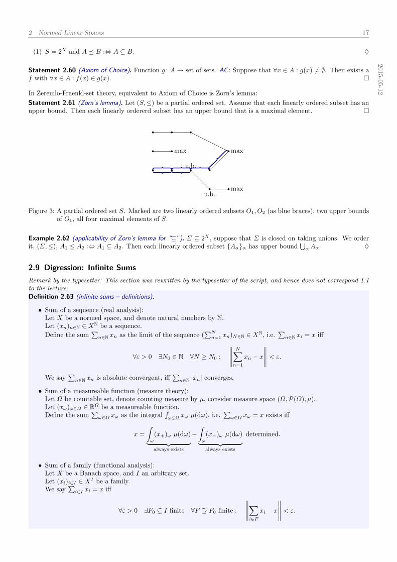
2 Normed Linear Spaces 17
(1) S = 2X and A B :⇔ A ⊆ B. ♦
2015-0
5-1
2
Statement 2.60 (Axiom of Choice). Function g : A→ set of sets. AC : Suppose that ∀x ∈ A : g(x) 6= ∅. Then exists af with ∀x ∈ A : f(x) ∈ g(x).
In Zeremlo-Fraenkl-set theory, equivalent to Axiom of Choice is Zorn’s lemma:
Statement 2.61 (Zorn’s lemma). Let (S,≤) be a partial ordered set. Assume that each linearly ordered subset has anupper bound. Then each linearly ordererd subset has an upper bound that is a maximal element.
max max
u.b.
u.b.max
Figure 3: A partial ordered set S. Marked are two linearly ordered subsets O1, O2 (as blue braces), two upper boundsof O1, all four maximal elements of S.
Example 2.62 (applicability of Zorn’s lemma for “⊆”). Σ ⊆ 2X , suppose that Σ is closed on taking unions. We orderit, (Σ,≤), A1 ≤ A2 :⇔ A1 ⊆ A2. Then each linearly ordered subset Aαα has upper bound
⋃αAα. ♦
2.9 Digression: Infinite Sums
Remark by the typesetter: This section was rewritten by the typesetter of the script, and hence does not correspond 1:1to the lecture.
Definition 2.63 (infinite sums – definitions).
• Sum of a sequence (real analysis):Let X be a normed space, and denote natural numbers by N.Let (xn)n∈N ∈ XN be a sequence.
Define the sum∑n∈N xn as the limit of the sequence (
∑Nn=1 xn)N∈N ∈ XN, i.e.
∑n∈N xi = x iff
∀ε > 0 ∃N0 ∈ N ∀N ≥ N0 :
∥∥∥∥∥N∑n=1
xn − x
∥∥∥∥∥ < ε.
We say∑n∈N xn is absolute convergent, iff
∑n∈N |xn| converges.
• Sum of a measureable function (measure theory):Let Ω be countable set, denote counting measure by µ, consider measure space (Ω,P(Ω), µ).Let (xω)ω∈Ω ∈ RΩ be a measureable function.Define the sum
∑ω∈Ω xω as the integral
∫ω∈Ω xω µ(dω), i.e.
∑ω∈Ω xω = x exists iff
x =
∫ω
(x+)ω µ(dω)︸ ︷︷ ︸always exists
−∫ω
(x−)ω µ(dω)︸ ︷︷ ︸always exists
determined.
• Sum of a family (functional analysis):Let X be a Banach space, and I an arbitrary set.Let (xi)i∈I ∈ XI be a family.We say
∑i∈I xi = x iff
∀ε > 0 ∃F0 ⊆ I finite ∀F ⊇ F0 finite :
∥∥∥∥∥∑i∈F
xi − x
∥∥∥∥∥ < ε.
2 Normed Linear Spaces 18
We say∑i∈I xi is absolute convergent, iff
∑n∈I |xi| converges.
Lemma 2.64 (infinite sums – equivalance of the definitions). In the notation of definition 2.63 (denote (I) := i ∈I | xi 6= 0):∑
n∈Nxn
convergent, but notabsolute convergent
⇒ ∀x ∈ X ∃J : N→ N bijection :∑n∈N
xJ(n) = x
[only forX = R!
]∑n∈N
xn absolute convergent ⇒ ∀J : N→ N bijection :∑n∈N
xJ(n) =∑n∈N
xn
∑ω∈Ω
xω determined ⇔ ∃J : N→ Ω bijection :∑n∈N
xJ(n)absoluteconvergent∑
x∈Ixi absolute convergent ⇔ ∃J : N→ (I) bijection :
∑n∈N
xJ(n)absoluteconvergent
Note that the latter “∃J : N→ (I) bijection” says that, in this case, at most countable xi’s are nonzero.
Prop. 2.65 (properties of the “functional analysis definition”).
(a) If ∀i ∈ I : xi ≥ 0, then∑i∈I xi converges if and only if supF⊆I finite
∑i∈F xi <∞.
(b) If ∀i ∈ I : xi ≥ 0 and∑i∈I xi converges, then only countable many xi’s are nonzero.
Proof. Proof of (b): Let In = i ∈ I | xi > 1n. Then
⋃n∈N In = i ∈ I | xi > 0. If the righthand side is uncountable,
then there exists a N such that IN is infinite. Then clearly supF⊆In∑i∈F xi =∞.
2.10 Bases of Hilbert Spaces
Definition 2.66 (orthonormal basis). An orthonormal set S = eαα∈A, eα ∈ H, then S is called an orthonormal basis,if any orthonormal set S′ ⊆ S implies S′ = S.
Remark 2.67. An orthonormal basis don’t have to be a (linear algebra) basis of H. //
Theorem 2.68 (every Hilbert space has an orthonormal basis). Every Hilbert space has an orthonormal basis.
Proof. Let S1, S2 be two orthonormal sets. We order them by inlusion, S1 ≤ S2 if S1 ⊆ S2. (Set of all orthonormal sets,≤)is a partially ordered set. Each linearly ordered chain Sαα∈I then
⋃α∈I Sα is an upper bound. It follows with Zorn’s
lemma that there exists a maximal orthonormal set S. Being maximal means that if S′ ⊆ S then S′ = S.
Theorem 2.69 (properties of orthonormal basis). Let S = eαα∈A be an orthonormal basis. Then the following holds:
(1) Coordinate representation: Every vector x ∈ H can be represented as
x =∑α∈A
eα〈eα, x〉.
(2) Parseval identity: For every vector x ∈ H, the so called Parseval identity holds,
‖x‖2 =∑α∈A|〈eα, x〉|2.
(3) Let (cα)α∈A ∈ FA be an arbitrary family. Then (both sums in the “functional analysis”-sense)∑α∈A
cα2 < converges︸ ︷︷ ︸
“coordinates” converges absolutely
⇒∑α∈A
cαeα converges︸ ︷︷ ︸“infinite linear combination” converges
.
Proof. Let F ⊆ A be a finite set, then by Bessel inequality,∑α∈F |〈eα, x〉|2 ≤ ‖x‖2, and therefore∑
α∈A|〈eα, x〉|2 ≤ ‖x‖2 converges.

2 Normed Linear Spaces 19
By virtue of (b) above, it follows that 〈eα, x〉 6= 0 only for countable many elements, α1, α2, α3, . . . . We have∑j∈N|〈eα, x〉|2 ≤ ‖x‖2. We claim xn :=
∑nj=1 eαj 〈eαj , x〉 is Cauchy sequence. Let n ≥ m. Then
‖xn − xm‖2 =
∥∥∥∥∥∥n∑
j=m
eαj⟨eαj , x
⟩∥∥∥∥∥∥2 =
m∑j=n
∣∣⟨eαj , x⟩∣∣2,
and hence (xn)n is a Cauchy sequence. Because H is a Banach space, it follows that xn −→ x.⟨eαj , x− x
⟩= limN→∞
⟨eαj , x− xN
⟩= limN→∞
⟨eαj , x−
N∑k=1
eαk〈eαk , x〉
⟩=⟨eαj , x
⟩−⟨eαj , x
⟩= 0
If α 6= αj , then also 〈eα, x − x〉 = 0. Then for all α ∈ A, eα ∈ S, 〈eα, x − x〉 = 0. Therefore x − x = 0, becauseotherwise S ∪ x−x
‖x−x‖ is an orthonormal set.∥∥∥∥∥∥x−N∑j=1
⟨eαj , x
⟩eαj
∥∥∥∥∥∥2 =
⟨x−
N∑j=1
⟨eαj , x
⟩eαj , x−
N∑k=1
〈eαk , x〉eαk
⟩
= ‖x‖2 − 2
N∑k=1
∣∣〈eαk , x〉∣∣2 +
N∑k=1
∣∣〈eαk , x〉∣∣2= ‖x‖2 −
N∑k=1
∣∣〈eαk , x〉∣∣20 = lim
N→∞
∥∥∥∥∥x−N∑k=1
eαk〈eαk , x〉
∥∥∥∥∥2
= limN→∞
(‖x‖2 −
N∑k=1
∣∣eαk〈eαk , x〉∣∣2) ∴ ‖x‖2 =
∞∑k=1
∣∣〈eαk , x〉∣∣2
Steps:
1. Only countable many cα is non-zero
2. Prove that partial sums∑Nj=1 cαjeαj is Cauchy
3. If Cauchy, then convergent.
2015-05-15
Recap:
Theorem 2.70 (characterization of orthonormal basis). Let S = eαα∈A be an orthonormal set. Then each of thefollowing statements is equivalent to “S is a basis”:
(i) ∀S′ orthonormal set : S′ ⊇ S ⇒ S′ = S
(ii) S⊥ = 0, i.e. ∀x ∈ H : (∀α ∈ A : 〈x, eα〉 = 0) ⇒ x = 0
(iii) spanS = H
(iv) ∀x ∈ H : ‖x‖2 =∑α∈A|〈x, eα〉|2
(v) ∀x ∈ H : x =∑α∈A eα〈eα, x〉
(vi) ∀x, y ∈ H : 〈x, y〉 =∑α∈A 〈eα, x〉 · 〈eα, y〉
Proof. We proved the hard parts in the last lecture.
2 Normed Linear Spaces 20
“(v) ⇒ (vi)”:
〈x, y〉 =
⟨∑α
eα〈eα, x〉,∑β
eβ〈eβ , y〉
⟩=∑α,β
〈eα, x〉 · 〈eβ , y〉 · 〈eα, eβ〉
=∑α
〈eα, x〉 · 〈eα, y〉
limN→∞
⟨N∑j=1
eαj⟨eαj , x
⟩,
N∑k=1
eβk〈eβk , x〉
⟩=
⟨ ∞∑j=1
eαj⟨eαj , x
⟩,
∞∑k=1
eβk〈eβk , x〉
⟩
Definition 2.71 (separable space). A topological space X is called separable, if it contains a countable dense subset S,
S = xn∞n=1 ∈ XN and S = X.
Algorithm 2.72 (Gram-Schmidt orthonormalization). Let vn∞n=1 be a set of independent vectors. Define recursively:
w1 = v1, e1 =w1
‖w1‖
wn+1 = vn+1 −n∑j=1
ej〈ej , vn+1〉, en+1 =wn+1
‖wn+1‖
Then:
(1) ejNj=1 is orthonormal
(2) spanvjnj=1 = spanejnj=1 for any 1 ≤ n ≤ N
Theorem 2.73 (characterization of separable Hilbert spaces). A Hilbert space is separable iff it has countable orthogonalbasis.
Proof. Proof of “⇒”: xn∞n=1 = H
1. Get sequence vnNn=1 (where N ∈ N0 ∪ ∞) of linearly independent vectors such that vnNn=1 = H
2. Now do Gram-Schmidt orthgonalization process to get S = en∞n=1, by construction span(S) = H
Proof of “⇐”: Consider alls rational finite linear combinations of basis vectors (see exercise).
Corollary 2.74 (coordinate representation is isometry). A separable infinite-dimensional Hilbert space H is isometric to`2. A finite-dimensional Hilbert space is isometric to Cn for some n.
Proof. Separable Hilbert space has a basis en∞n=1. Define map
H → `2, x 7→ 〈en, x〉∞n=1,
then:
• Well-defined because of Bessel inequality
• Isometry because of Parseval identity (‖x‖H = ‖〈en, x〉∞n=1‖`2)
• Bijective because of . . .
2.11 [Digression] Applications
2.11.1 Measure theory
2 Normed Linear Spaces 21
Theorem 2.75 (Radon-Nikodym). Let µ, ν be finite measures on a measureable space (X,Σ). Suppose that ν isabsolutely continuous w.r.t. µ, then there exists a g µ-measureable and g ≥ 0 such that
∀E ∈ Σ : ν(E) =
∫E
g dµ ,
what is equivalent to ∫X
f dν =
∫X
(f · g)dµ.
g is called the Radon-Nikodym derivative, “dν = g dµ”.
Remark 2.76. The theorem also holds for σ-finite measures. Recall:– Finite: µ(X), ν(X) <∞– σ-finite: . . .– Absolutely continuous ν µ: ∀F ∈ Σ : µ(F ) = 0 ⇒ ν(F ) = 0 //
Proof by von Neumann. L2(X,µ+ ν) is a (real) Hilbert space,
〈f, g〉 =
∫X
(f · g) (dν + dµ), ‖f‖ =
√∫X
f2 (dν + dµ).
Consider a functional f 7→∫Xf dµ. Claim: This is a bounded functional H → R.∣∣∣∣∫X
f dµ
∣∣∣∣ ≤√∫
X
f2 dµ ·
√∫X
dµ ≤
√∫X
f2 (dµ+ dν) · µ(X)
By virute of the Riesz representation theorem (“H? = H”), there exists a function h such that∫X
f dµ =
∫X
(fg) (dµ+ dν)∫x
f(1− h) dµ =
∫X
(fh) dν. (∗)
Define function f such that f = f 1h . Claim 0 < h ≤ 1 almost surely:
• Let F := x | h(x) ≤ 0. Put f = characteristic function of F into (∗):
µ(F ) ≤∫F
(1− h) dµ =
∫F
h dν ≤ 0 ∴ µ(F ) ≤ 0 ∴ µ(F ) = 0 ∴ ν(F ) = 0 ∴ (µ+ ν)(F ) = 0
• Let F = x | h(x) > 1. Put characterisitic function of F into (∗),∫F
(1− h) dµ =
∫F
hdν.
Suppose that µ(F ) > 0, then the left hand side is negative, but the right hand side is non-negative. Contradiction,hence µ(F ) = 0, and therefore (µ+ ν)(F ) = 0.
Put f = f 1h into (∗), ∫
X
f1− hh
dµ =
∫X
f dν.
Conclusion: g = 1−hh satisfies the theorem.
2.11.2 Fourier transform
Classical result in Fourier theory :
Definition 2.77 (Fourier coefficients). To each function f , define the fourier coefficients of f to be
cn :=1√2π
∫ +π
−πeinxf(x) dx, n ∈ Z.
2 Normed Linear Spaces 22
Theorem 2.78 (Fourier series – classical viewpoint). For every 2π-periodic function f ∈ C(]−π,+π[), its Fourier seriesconverges uniformly to f ,
1√2π
+N∑j=−N
cjeijx N→∞−−−−−−→
uniformlyf(x).
Theorem 2.79 (Fourier series – functional analysis viewpoint). Consider the space L2(]−1,+1[). Then (en)n∈N, en(x) =1√2π
einx is an orthonormal basis of L2(]−1,+1[), i.p. ∀m 6= n : 〈em, en〉 = 0 and ∀n : 〈en, en〉 = 1. Therefore, for
every function f ∈ L2(]−1,+1[)
∑n
cnen −−−−−→L2-conv.
f where cn := 〈en, f〉 i.e. f =====L2-eq.
n=+∞∑n=−∞
en〈en, f〉,
where the latter equality is in the L2-sense, not pointwise equality.
Proof. Use Stone-Weierstrass theorem, to get that S = en∞n=1 is dense in C(]−π,+π[).
3 Bounded Operators 23
BoundedOperators 3
3.1 Bounded Linear Maps
2015-0
5-1
9
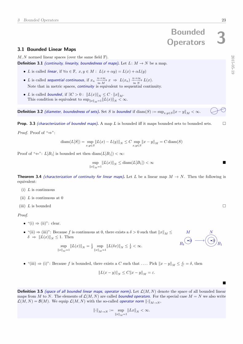
M,N normed linear spaces (over the same field F).
Definition 3.1 (continuity, linearity, boundedness of maps). Let L : M → N be a map.
• L is called linear , if ∀α ∈ F, x, y ∈M : L(x+ αy) = L(x) + αL(y)
• L is called sequential continuous, if xnn→∞−−−−→in M
x ⇒ L(xn)n→∞−−−−→in N
L(x).
Note that in metric spaces, continuity is equivalent to sequential continuity.
• L is called bounded , if ∃C > 0 : ‖L(x)‖N ≤ C · ‖x‖M .This condition is equivalent to sup‖x‖M=1‖L(x)‖N <∞.
Definition 3.2 (diameter, boundedness of sets). Set S is bounded if diam(S) := supx,y∈S‖x− y‖M <∞.
Prop. 3.3 (characterization of bounded maps). A map L is bounded iff it maps bounded sets to bounded sets.
Proof. Proof of “⇒”:
diam(L[S]) = supx,y∈S
‖L(x)− L(y)‖N ≤ C supx,y∈S
‖x− y‖M = C diam(S)
Proof of “⇐”: L[B1] is bounded set then diam(L[B1]) <∞:
sup‖x‖M=1
‖L(x)‖N ≤ diam(L[B1]) <∞
Theorem 3.4 (characterization of continuity for linear maps). Let L be a linear map M → N . Then the following isequivalent:
(i) L is continuous
(ii) L is continuous at 0
(iii) L is bounded
Proof.
• “(i) ⇒ (ii)”: clear.
• “(ii)⇒ (iii)”: Because f is continuous at 0, there exists a δ > 0 such that ‖x‖M ≤δ ⇒ ‖L(x)‖N ≤ 1. Then
sup‖x‖M=1
‖L(x)‖N = 1δ sup‖x‖M=1
‖L(δx)‖N ≤1δ <∞.
M
0Bδ
N
0B1
• “(iii) ⇒ (i)”: Because f is bounded, there exists a C such that . . . . Pick ‖x− y‖M ≤εC = δ, then
‖L(x− y)‖N ≤ C‖x− y‖M = ε.
Definition 3.5 (space of all bounded linear maps, operator norm). Let L(M,N) denote the space of all bounded linearmaps from M to N . The elements of L(M,N) are called bounded operators. For the special case M = N we also writeL(M,N) = B(M). We equip L(M,N) with the so-called operator norm ‖·‖M→N ,
‖·‖M→N := sup‖x‖M=1
‖Lx‖N <∞.
3 Bounded Operators 24
Definition 3.6 (dual space). Recall definition 3.5 and consider the special case N = F (where F = R or C). ThenL(M,F) = M∗ is the dual space of M , and the elements of L(M,F) are the linear functionals on M .
Recall:
Definition 2.48 (dual space). A map ϕ : H → C is called a linear functional , if it is a bounded linear map, i.e.:(1) Linearity: ∀x, y ∈ H, α ∈ C : ϕ(x+ αy) = ϕ(x) + αϕ(y)(2) Boundedness: ∃C ∈ R : |ϕ(x)| ≤ C‖x‖H
The space of all linear functionals on H is called the dual space H∗ of H. We equip H∗ with a norm ‖·‖H∗ ,
‖ϕ‖H∗ := supx∈H,‖x‖=1
|ϕ(x)| = supx∈H,x 6=0
|ϕ(x)|‖x‖
.
Remark 2.49. Remark by the typesetter: This definition holds for any normed space, not just Hilbert spaces. Anyway,the more general definition will come in definition 3.6. Furhtermore, the norm ‖·‖M∗ conincides with the operatornorm ‖·‖M→F. //
Notation 3.7. Sometimes, we omit braces “(”, “)” and the composition symbol “”:
• For L : M → N linear map and x ∈M , we write L(x) := Lx.
• For L1 : M1 →M2 and L2 : M2 →M3, we write L2L1 := L2 L1 : M1 →M3. //
Two inequalities about ‖·‖M→N :
Theorem 3.8 (submultiplicativity of the operator norm).
(1) ‖Lx‖N ≤ ‖L‖M→N‖x‖M .
(2) ‖L2L1‖M1→M3≤ ‖L2‖M2→M3
‖L1‖M1→M2
Proof.
(1) ‖Lx‖N ≤ sup‖y‖M=1
L (y‖x‖M ) = ‖x‖M‖L‖M→N
(2) ‖L2L1‖M1→M3= sup‖x‖M1
=1
‖L2L1x‖M3≤ sup‖x‖M1
=1
‖L2‖M2→M3‖L1x‖M2
= ‖L2‖M2→M3‖L1‖M1→M2
Theorem 3.9 (properties of L(M,N)). The space (L(M,N), ‖·‖M→N ) is a normed linear space. And if N is a Banachspace, then so is L(M,N).
Proof. ‖·‖M→N is a norm:
‖L1 + L2‖M→N = sup‖x‖M=1
‖(L1 + L2)x‖N ≤ sup‖x‖M=1
‖L1x‖N + sup‖x‖M=1
‖L2x‖N = ‖L1‖M→N + ‖L2‖M→N
Consider Cauchy sequence (Ln)∞n=1,‖Ln − Lk‖M→N ≤ ε if n, k is large.
Then for each x ∈M , (Lnx)n is Cauchy sequence in N ,
‖Lnx− Lkx‖N ≤ ‖Ln − Lk‖M→N‖x‖M ≤ ε‖x‖M .
Because N is a Banach space, it follows that Lx := limn→∞ Lnx exists for each x ∈M .
• Linearity: L(x+ y) = limn→∞ Ln(x+ y) = limn→∞ Lnx+ Lny = Lx+ Ly
• Boundedness: Observe (‖Ln‖M→N )n is a Cauchy sequence, |‖L‖ − ‖L‖| ≤ ‖L − L‖. If (‖Ln‖M→N )n isCauchy, then there is a C > 0 such that ∀n ∈ N : ‖Ln‖M→N ≤ C. Then we have sup‖x‖M=1‖Lx‖N =
sup‖x‖M=1 limn→∞‖Lnx‖N ≤ sup‖x‖M=1 limn→∞ C‖x‖M = C <∞.
Let n be such that for all k ≥ n it holds that
∀x ∈M : limk→∞
‖(Ln − Lk)x‖N ≤ ε‖x‖M∴ ‖(Ln − L)x‖N ≤ ε‖x‖M∴ sup
‖x‖M=1
‖(Ln − L)x‖N ≤ ε
∴ ‖Ln − L‖M→N ≤ ε
3 Bounded Operators 25
Example 3.10 (examples of linear maps).
(1) Consider M = C([−1,+1]) and a linear functional ϕ ∈ M∗ defined by ϕ(f) = f(0). Then |ϕ(f)| ≤ ‖f‖M , andhence ‖ϕ‖M? ≤ 1, and actually ‖ϕ‖M? = 1.
(2) Consider M = C([0,+1]) and continuous function K : [0,+1]× [0,+1] → C, then (Lf)(x) :=∫ 1
0K(x, y)f(y) dy
is an operator in L(M).
‖Lf‖M = supx∈[0,1]
|(Lf)(x)| = supx∈[0,1]
∣∣∣∣∫ 1
0
K(x, y)f(y) dy
∣∣∣∣ ≤ supx,y∈[0,1]
|K(x, y)|‖f‖M ∴ ‖L‖M→M ≤ supx,y∈[0,1]
|K(x, y)|
♦
2015-0
5-2
2
Question: Let L : M → N be a bounded norm, L ∈ L(M,N), and consider the norm ‖·‖M→N . Is ‖L‖M→N =supx∈M,‖x‖M≤1‖Lx‖N a correct relation?
3.2 Digression: Unbounded operators
2015-0
5-1
9
Remark 3.11 (unbounded maps).
• unbounded 6= not bounded
• unbounded = not defined everywhere (very important)
• discontinuous = not bounded (obscurity) //
Definition 3.12 (Hamel basis). Hamel basis (algebraic basis) of M : This is a set S = eαα∈A satisfying:
• Any finite subset of S is linearly independent
• All x ∈M can be uniquely written as finite linear combination of eαα∈A
Prop. 3.13 (every linear space has an algebraic basis). Every normed linear space M has an algebraic basis.
Remark 3.14. If M is a Banach space and dimM =∞, then the Hamel basis is uncountable. //
Prop. 3.15 (existence of discontinuous maps). Not bounded maps do exist.
Proof. Let M be a Banach space of dimM = ∞. Pick a countable sequence (eαn)∞n=1 (w.l.o.g. ‖eαn‖ = 1). DefineL : M → C by Leαn = n, and Leα = 0 if eα 6= eαn for any n, and linearity. Then L is linear, but clearly notbounded.
3.3 The Dual Space of a `p-Space
2015-05-22
Consider `p, at first only p ∈ ]1,∞[, and p ∈ 1,∞ later.
Theorem 3.16 (Holder inequality). For x ∈ `p and y ∈ `q, where p, q conjugate numbers, e.g. 1p + 1
q = 1, then∣∣∣∣∣∞∑n=1
xnyn
∣∣∣∣∣ ≤( ∞∑n=1
|xn|p)1/p
·
( ∞∑n=1
|xn|q)1/q
= ‖x‖p · ‖y‖q.
Proof. Omitted.
Lemma 3.17 (every vector in `q induces a linear functional in (`p)∗). For y ∈ `q, define
ϕ : `p → C, ϕy(x) :=
∞∑n=1
xnyn.
Then ϕy ∈ (`p)∗, i.e. ϕy is bounded.
3 Bounded Operators 26
Proof.
‖ϕy‖ = sup‖x‖p=1
|ϕy(x)| = sup‖x‖p=1
∣∣∣∣∣∞∑n=1
xnyn
∣∣∣∣∣ ≤ sup‖x‖p=1
‖x‖p‖y‖q = ‖y‖q
Lemma 3.18 (norm of induced functional). For every y ∈ `q, it holds that
‖ϕy‖(`p)∗ = ‖y‖`q .
Proof. From the proof of lemma 3.17 we know ‖ϕy‖(`p)∗ ≤ ‖y‖`q . Furthermore, for any ‖z‖p = 1, ‖ϕy‖ = sup‖x‖p=1|ϕy(x)| ≥|ϕy(z)|. We claim that equality is achieved if |xn|p = |yn|q, i.e. |xn| = |yn|q/p. Proof of claim: Take z = |yn|q/p sgn(yn),then z ∈ `p, because ‖z‖pp =
∑∞n=1|yn|q = ‖y‖qq. Take z = z
‖y‖qq/p, then
ϕy(z) =
∞∑n=1
|yn|q/p
‖y‖qq/p= ‖y‖q
−q/p∞∑n=1
|yn|q/p+1 = ‖y‖q−q/p‖y‖q
q = ‖y‖q.
We conclude ‖ϕy‖(`p)∗ = ‖y‖`q .
Lemma 3.19 (duality between p- and q-norm).
‖x‖p = sup‖y‖q=1
∣∣∣∣∣∞∑n=1
xnyn
∣∣∣∣∣ = sup‖y‖q=1
|ϕy(x)|
Proof. Righthand side issup‖y‖q=1
|ϕy(x)| ≤ sup‖y‖q=1
‖ϕy‖‖x‖p = ‖x‖p.
Pick yn = |xn|p/q sgn(xn), then ‖x‖p = sup‖y‖q=1|ϕy(x)|.
Lemma 3.19 can be used in convex optimization. Another application of lemma 3.19 is proving that the p-norm ‖·‖pis indeed a norm.
Corollary 3.20 (Minkowsi inequality = triangle inequality for ‖·‖p). ‖·‖p satisfies the triangle inequality.
Proof.‖x1 + x2‖p = sup
‖y‖q=1
|ϕy(x1 + x2)| ≤ sup‖y‖q=1
(|ϕy(x1)| + |ϕy(x2)|
)= ‖x1‖p + ‖x2‖p
Corollary 3.21 (p-norm is a norm). From corollary 3.20 it follows that ‖·‖p is a norm.
Lemma 3.22 (every linear functional in (`p)∗ is induced by a vector in `q). For all ϕ ∈ (`p)∗, there exists a y ∈ `q suchthat ∀x ∈ `p : ϕ(x) = ϕy(x).
Proof. Let ϕ ∈ (`p)∗ and e1 = (1, 0, 0, . . . ), e2 = (0, 1, 0, . . . ), etc.. Define y by yn := ϕ(en). Things to check:
1. y ∈ `q:
‖y‖q = sup‖x‖p=1
∣∣∣∑xnyn
∣∣∣ = sup‖x‖p=1
∣∣∣∣∣∞∑n=1
xnϕ(en)
∣∣∣∣∣ = sup‖x‖p=1
|ϕ(x)| ≤ ‖ϕ‖ <∞
2. ϕ = ϕy:By construction ϕ = ϕy on ccpt ⊆ `p. We know that ccpt is dense in `p, p < ∞, so it follows that ϕ = ϕy (ifcontinuous map coincide on a dense subset, then they are the same everywhere).
Corollary 3.23 ((`p)∗ is isomorphic to `q). (`p)∗ is isomorphic to `q: By lemma 3.17 and lemma 3.22 every vector y ∈ `qcorresponds to a linear functional ϕ ∈ (`p)∗ (via y 7→ ϕy), and vice versa. Furthermore, by lemma 3.18 this bijection(y 7→ ϕy) is isometric.
Remark 3.24.
‖ϕy‖(`p)∗ = supx∈`p,‖x‖`p=1
|ϕy(x)| by definition
‖x‖`p = supϕ∈(`p)∗,‖ϕ‖(`p)∗=1
|ϕ(x)| by claim
3 Bounded Operators 27
//
Remark 3.25. (“∼=” means isometric)
• (`1)∗ ∼= `∞
• (`∞)∗ is more complicated, since ccpt is not dense in `∞
• (Lp(X,Σ, µ))∗ ∼= Lq(X,∑, µ) for p ∈ ]1,∞[
• (L1(X,Σ, µ))∗ ∼= L∞(X,∑, µ) if µ is σ-finite
• (L∞(X,Σ, µ))∗ ∼= bq(X,∑
) = space of all σ-finite bounded measures ν << µExample: (L∞([−1,+1])∗ constains inter alia of:
– For any g ∈ L1([−1,+1]), f 7→∫ +1
−1
∫ +1
−1f(x) · g(x) dx
– Measures: “δ-function: f 7→ f(0)”
//
3.4 Hahn-Banach Theorem
Prop. 3.26. Let M be a normed linear space and x ∈M .
‖x‖ = supϕ∈M∗,‖ϕ‖=1
|ϕ(x)|
Proof of proposition 3.26 – Part 1/2. Steps:
1. sup‖ϕ‖=1|ϕ(x)| ≤ sup‖ϕ‖=1‖ϕ‖‖x‖ = ‖x‖
2. Try to find ‖ϕ‖ = 1 such that ϕ(x) = ‖x‖.
This is a constrait on Y = λx | λ ∈ F. We finish the proof later.
Theorem 3.27 (Hahn-Banach theorem – real version). Let X be a linear space and p a function X → R that satisfies
(i) positive homogeniety: ∀x ∈ X,α > 0 : p(αx) = αp(x), and
(ii) sub-additivity: ∀x, y ∈ X : p(x+ y) ≤ p(x) + p(y).
Let ϕ be a linear functional defined on Y ⊆ X, where Y is a linear subspace, such that
∀y ∈ Y : ϕ(y) ≤ p(y).
Then there exists an extension of ϕ to X such that ∀x ∈ X : ϕ(x) ≤ p(x).
Remark 3.28.
• If p is absolute homogeneous, i.e. ∀α ∈ R : p(αx) = |α|p(x), then p is a pseudo-norm, i.e. a norm without∀x ∈ X : p(x) = 0⇒ x = 0.
• Typically, p is a norm. //
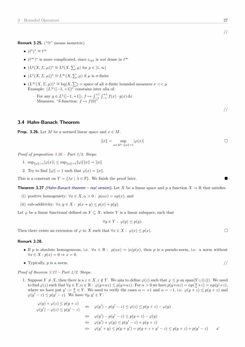
Proof of theorem 3.27 – Part 1/2. Steps:
1. Suppose Y 6= X, then there is a z ∈ X, z /∈ Y . We aim to define ϕ(z) such that ϕ ≤ p on span(Y ∪z). We needto find ϕ(z) such that ∀y ∈ Y, α ∈ R : ϕ(y+αz) ≤ p(y+αz). For α > 0 we have p(y+αz) = αp( yα+z) = αp(y′+z),where we have put y′ := y
α ∈ Y . We need to verify the cases α = +1 and α = −1, i.e. ϕ(y + z) ≤ p(y + z) andϕ(y′ − z) ≤ p(y′ − z). We have ∀y, y′ ∈ Y :
ϕ(y) + ϕ(z) ≤ p(y + z)
ϕ(y′)− ϕ(z) ≤ p(y′ − z)⇔ ϕ(y′)− p(y′ − z) ≤ ϕ(z) ≤ p(y + z)− ϕ(y)
⇔ ϕ(y′)− p(y′ − z) ≤ p(y + z)− ϕ(y)
⇔ ϕ(y′) + ϕ(y) ≤ p(y′ − z) + p(y + z)
⇔ ϕ(y′ + y) ≤ p(y + y′) = p(y + z + y′ − z) ≤ p(y + z) + p(y′ − z) X
3 Bounded Operators 28
2. Next lecture.
2015-0
5-2
9
Repitition: Hahn-Banach theorem (real version): Let X be a real linear space and p : X → R satisfiying:
(i) ∀α > 0 : p(αx) = αp(x)
(ii) p(x+ y) ≤ p(x) + p(y)
Let Y be a linear subspace of X and ϕ a functional on Y such that
∀y ∈ Y : ϕ(y) ≤ p(y), (∗)
then there exists an extension of ϕ to all X such that ϕ is linear and ∀x ∈ X : ϕ(x) ≤ p(x).
Proof of theorem 3.27 – Part 2/2. Steps:
1. For any z /∈ y, there exists an extension to span(Y ∪ z), such that (∗) holds on span(Y ∪ z).
2. Apply Zorn’s lemma: Let (W,ϕ) be a set of all extensions (that satisfy (∗)), is partially ordered by (W,ϕ) (W ′, ϕ′) if W ⊆ W ′ and ϕ = ϕ′ on W . All satisfy W ⊇ Y and φ in Y is as in the theorem. Let (Wα, ϕα) be
a linearly ordered subset, then W :=⋃α∈AWα and ϕ(x) =
ϕα(x) for x ∈Wα . We need to check ∀α ∈ A :
(Wα, ϕα) ≺ (W,ϕ), but by construction Wα ⊆W and ϕ = ϕα on Wα, so (W,ϕ) is an upper bound. By virtue ofZorn’s lemma, the set of extension has a maximal element. Let (W , ϕ) be a maximal element, then W = X.
Theorem 3.29 (Hahn-Banach theorem – complex version). Let X be a complex linear space and p : X → R a pseudo-norm (i.e. change condition 3.27.(i) to ∀α ∈ C : p(αx) = |α|p(x)). Let Y be a linear subspace of X and ϕ a linearfunctional on Y such that ∀y ∈ Y : |ϕ(y)| ≤ p(y). Then there exists an extension of ϕ to X such that ϕ is linear and∀x ∈ X : |ϕ(x)| ≤ p(x).
Proof. Similar to the proof of the real version.
Application of Hahn-Banach theorem:
Lemma 3.30 (existence of tangent). Let X be a normed linear space and x0 ∈ X. Then there exists a ϕ ∈ X∗ suchthat ‖ϕ‖ = 1 and ϕ(x0) = ‖x0‖.
Proof. Let x0 6= 0, and define Y = αx0 | α ∈ F and p : X → R, p(x) = ‖x‖. On Y define ϕ(αx0) = α‖x0‖. Then byHahn-Banach theorem, there exists a ϕ on X such that |ϕ(x)| ≤ ‖x‖ and ϕ(αx0) = α‖x0‖. By construction ‖ϕ‖ ≤ 1,but ϕ(x0) = ‖x0‖, and hence ‖ϕ‖ = 1.
Definition 3.31 (hyperplane, half space, tangent). Let X be a real vectorspace.
A subspace Y ⊆ X is called a hyperplane, if there exists ϕ ∈ X∗ and α ∈ R such thatY = x ∈ X | ϕ(x) = α =: ϕ = α. Sets x ∈ X | ϕ(x) < α, resp. x ∈ X | ϕ(x) > α arecalled open half spaces.
ϕ = 0
ϕ = α
0
A tangent to a set K at a point x0 ∈ K is a hyperplane Y = ϕ = α such that x0 ∈ Y andK ⊆ ϕ ≤ α. Look at B1 = ‖x‖ ≤ 1. We have any ‖x0‖ = 1, therefore there exists ϕ suchthat ϕ(x0) = 1 and for x ∈ B1 ϕ(x) ≤ 1.
x0
Remark 3.32 (uniqueness in Hahn-Banach theorem). Concering lemma 3.30:
x0
x0
x0 x01
Figure 4: Tangents to subspaces of R2
Middle figure: At some point there may be more than one tangent.
3 Bounded Operators 29
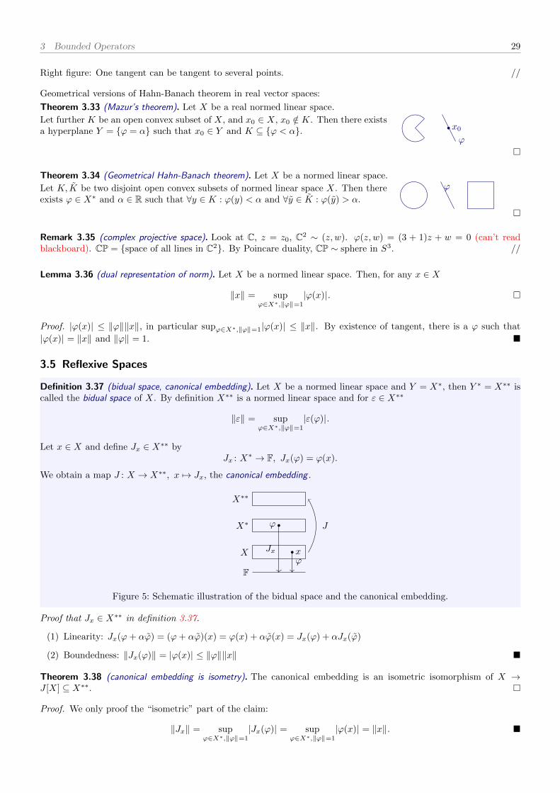
Right figure: One tangent can be tangent to several points. //
Geometrical versions of Hahn-Banach theorem in real vector spaces:
Theorem 3.33 (Mazur’s theorem). Let X be a real normed linear space.
Let further K be an open convex subset of X, and x0 ∈ X, x0 /∈ K. Then there existsa hyperplane Y = ϕ = α such that x0 ∈ Y and K ⊆ ϕ < α.
ϕ
x0
Theorem 3.34 (Geometrical Hahn-Banach theorem). Let X be a normed linear space.
Let K, K be two disjoint open convex subsets of normed linear space X. Then thereexists ϕ ∈ X∗ and α ∈ R such that ∀y ∈ K : ϕ(y) < α and ∀y ∈ K : ϕ(y) > α.
ϕ
Remark 3.35 (complex projective space). Look at C, z = z0, C2 ∼ (z, w). ϕ(z, w) = (3 + 1)z + w = 0 (can’t readblackboard). CP = space of all lines in C2. By Poincare duality, CP ∼ sphere in S3. //
Lemma 3.36 (dual representation of norm). Let X be a normed linear space. Then, for any x ∈ X
‖x‖ = supϕ∈X∗,‖ϕ‖=1
|ϕ(x)|.
Proof. |ϕ(x)| ≤ ‖ϕ‖‖x‖, in particular supϕ∈X∗,‖ϕ‖=1|ϕ(x)| ≤ ‖x‖. By existence of tangent, there is a ϕ such that
|ϕ(x)| = ‖x‖ and ‖ϕ‖ = 1.
3.5 Reflexive Spaces
Definition 3.37 (bidual space, canonical embedding). Let X be a normed linear space and Y = X∗, then Y ∗ = X∗∗ iscalled the bidual space of X. By definition X∗∗ is a normed linear space and for ε ∈ X∗∗
‖ε‖ = supϕ∈X∗,‖ϕ‖=1
|ε(ϕ)|.
Let x ∈ X and define Jx ∈ X∗∗ byJx : X∗ → F, Jx(ϕ) = ϕ(x).
We obtain a map J : X → X∗∗, x 7→ Jx, the canonical embedding .
F
X
X∗
X∗∗
x
ϕ
ϕ
Jx
J
Figure 5: Schematic illustration of the bidual space and the canonical embedding.
Proof that Jx ∈ X∗∗ in definition 3.37.
(1) Linearity: Jx(ϕ+ αϕ) = (ϕ+ αϕ)(x) = ϕ(x) + αϕ(x) = Jx(ϕ) + αJx(ϕ)
(2) Boundedness: ‖Jx(ϕ)‖ = |ϕ(x)| ≤ ‖ϕ‖‖x‖
Theorem 3.38 (canonical embedding is isometry). The canonical embedding is an isometric isomorphism of X →J [X] ⊆ X∗∗.
Proof. We only proof the “isometric” part of the claim:
‖Jx‖ = supϕ∈X∗,‖ϕ‖=1
|Jx(ϕ)| = supϕ∈X∗,‖ϕ‖=1
|ϕ(x)| = ‖x‖.

3 Bounded Operators 30
Remark 3.39 (linear isometries are injective). Linear isometries are always injective. //
2015-0
6-0
2
Definition 3.40 (reflexive space). Space X is called reflexive if J is surjective, i.e. J [X] = X∗∗.
Remark 3.41.
• Reflexive spaces are always complete, hence Banach.
• If J [X] ⊆ X∗∗ (Remark by the typesetter: this is always true), then J [X] is a Banach space. J [X] is a completitionof X.
• There exists a space X such that X and X∗∗ are isometrically isomorphic, but X is not reflexive.
//
Remark about completitions:
Definition 3.42 (completition). Let X be a normed linear space. A mapping φ : X → Y is called completition of X, ifY is complete, φ[X] is dense in Y , and φ is an isometric homomorphism. The pair (φ, Y ) is called completition of X.
Example 3.43 (standard completition). Consider the space of all Cauchy sequences (xn)n∈N in X and equip it with theequivalence relation
[(xn)n∈N] = [(xn)n∈N] ⇔ limn→∞
xn = limn→∞
xn.
Then put Y = [(xn)n∈N] | (xn)n∈N ∈ XN cauchy. ♦
Prop. 3.44 (Hilbert spaces are reflexive). All Hilbert spaces are reflexive.
Proof. Preliminary remark: X = H, X ∼= X∗ by Riesz duality:
Φ : H → H∗, Φ(x) = ϕx, ϕx(y) = 〈x, y〉
So(H∗)∗
Φ∼= H∗Φ∼= H.
Proof itself: Let Φ be a Riesz duality between H and H∗. H∗ itself is a Hilbert space, 〈ϕx, ϕy〉 = 〈y, x〉. Then we havea map
Φ : H∗ → H∗∗, ϕx 7→ Φ(ϕx) = εϕx , εϕx(ϕy) = 〈ϕx, ϕy〉.
We will check that Φ Φ = J :((Φ Φ)(x)
)(ϕy)
=(Φ(ϕx)
)(ϕy)
= εϕx(ϕy) = 〈ϕx, ϕy〉 = 〈y, x〉 = ϕy(x) = Jx(ϕy) ∴ Φ Φ = J
Example 3.45 (examples and counterexamples of reflexive spaces).
(1) Lp(X,Σ, µ) is reflexive for p ∈ ]1,∞[, in particular `p is reflexive for p ∈ ]1,∞[.(Lp)∗ = Lq, (Lq)∗ = Lp, 1
p + 1q = 1.
(2) L1 and L∞ are not reflexive.
(3) c0, c1, C([0, 1]) are not reflexive. ♦
3.6 The Conjugate of an Operator
Definition 3.46 (Banach conjugate). Let M,N be normed linear spaces and L ∈ L(M,N). Then the Banach conjugateL′ is a linear map L′ ∈ L(N∗,M∗) defined by ∀ϕ ∈ N∗, x ∈M : (L′(ϕ))(x) = ϕ(L(x)).
3 Bounded Operators 31
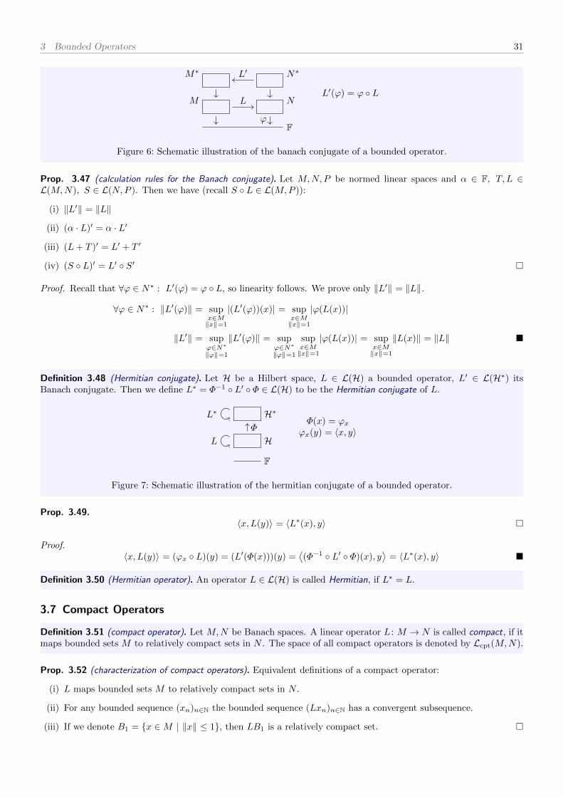
M∗ N∗
M N
Fϕ
L′
LL′(ϕ) = ϕ L
Figure 6: Schematic illustration of the banach conjugate of a bounded operator.
Prop. 3.47 (calculation rules for the Banach conjugate). Let M,N,P be normed linear spaces and α ∈ F, T, L ∈L(M,N), S ∈ L(N,P ). Then we have (recall S L ∈ L(M,P )):
(i) ‖L′‖ = ‖L‖
(ii) (α · L)′ = α · L′
(iii) (L+ T )′ = L′ + T ′
(iv) (S L)′ = L′ S′
Proof. Recall that ∀ϕ ∈ N∗ : L′(ϕ) = ϕ L, so linearity follows. We prove only ‖L′‖ = ‖L‖.
∀ϕ ∈ N∗ : ‖L′(ϕ)‖ = supx∈M‖x‖=1
|(L′(ϕ))(x)| = supx∈M‖x‖=1
|ϕ(L(x))|
‖L′‖ = supϕ∈N∗‖ϕ‖=1
‖L′(ϕ)‖ = supϕ∈N∗‖ϕ‖=1
supx∈M‖x‖=1
|ϕ(L(x))| = supx∈M‖x‖=1
‖L(x)‖ = ‖L‖
Definition 3.48 (Hermitian conjugate). Let H be a Hilbert space, L ∈ L(H) a bounded operator, L′ ∈ L(H∗) itsBanach conjugate. Then we define L∗ = Φ−1 L′ Φ ∈ L(H) to be the Hermitian conjugate of L.
H∗
H
F
Φ
L
L∗Φ(x) = ϕx
ϕx(y) = 〈x, y〉
Figure 7: Schematic illustration of the hermitian conjugate of a bounded operator.
Prop. 3.49.〈x, L(y)〉 = 〈L∗(x), y〉
Proof.〈x, L(y)〉 = (ϕx L)(y) = (L′(Φ(x)))(y) =
⟨(Φ−1 L′ Φ)(x), y
⟩= 〈L∗(x), y〉
Definition 3.50 (Hermitian operator). An operator L ∈ L(H) is called Hermitian, if L∗ = L.
3.7 Compact Operators
Definition 3.51 (compact operator). Let M,N be Banach spaces. A linear operator L : M → N is called compact, if itmaps bounded sets M to relatively compact sets in N . The space of all compact operators is denoted by Lcpt(M,N).
Prop. 3.52 (characterization of compact operators). Equivalent definitions of a compact operator:
(i) L maps bounded sets M to relatively compact sets in N .
(ii) For any bounded sequence (xn)n∈N the bounded sequence (Lxn)n∈N has a convergent subsequence.
(iii) If we denote B1 = x ∈M | ‖x‖ ≤ 1, then LB1 is a relatively compact set.
3 Bounded Operators 32
Definition 3.53 (finite-rank operator). A linear operator L : M → N is called finite-rank if L ∈ L(M,N) and im(F ) isa finite-dimensional space. The space of all finite-rank operators is denoted by Lf(M,N).
Prop. 3.54 (properties of Lcpt(M,N)). Let M,N be Banach spaces. Then:
(i) Lf(M,N) ⊆ Lcpt(M,N) ⊆ L(M,N).
(ii) If (Ln)n∈N is a sequence in Lcpt(M,N) and LNN→∞−→ L, i.e. ‖LN − L‖ N→∞−→ L, with L ∈ L(M,N), then
L ∈ Lcpt(M,N). I.e. Lcpt(M,N) is closed.
(iii) If L ∈ L(M,N), S ∈ L(N,P ), then S L ∈ L(M,P ) is compact if L or S is compact. I.e. Lcpt(M,N) is atwo-sided ideal in L(M,N).
Example 3.55 (Volterra integral operator is compact). The Volterra integral operator L : C([0, 1])→ C([0, 1]), (Lf)(x) =∫ x0K(x, y) · f(y) dy is compact. ♦
2015-0
6-0
5
Theorem 3.56 (properties of Lcpt(M,N)).
(i) Lf(M,N) ⊆ Lcpt(M,N) ⊆ L(M,N)
(ii) Lcpt(M,N) is a closed subspace of L(M,N)
(iii) Lcpt(M,N) is a two-sided ideal, i.e. for any T, L ∈ L(M,N), TL is compact whenever T or L is.
Proof.
(i) If L ∈ Lcpt(M,N) then LB1 is relatively compact hence bounded.
(ii) We need to prove that if Ln ∈ Lcpt and Lnn→∞−→ L, i.e. ‖Ln − L‖
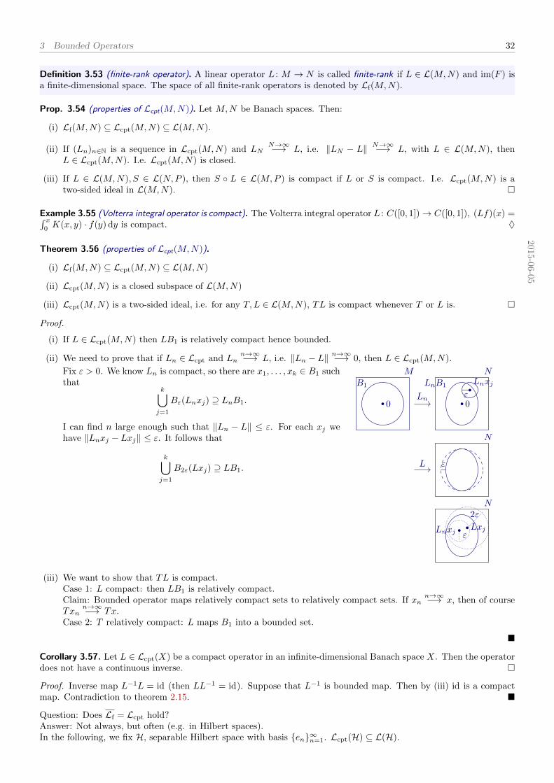
n→∞−→ 0, then L ∈ Lcpt(M,N).
Fix ε > 0. We know Ln is compact, so there are x1, . . . , xk ∈ B1 suchthat
k⋃j=1
Bε(Lnxj) ⊇ LnB1.
I can find n large enough such that ‖Ln − L‖ ≤ ε. For each xj wehave ‖Lnxj − Lxj‖ ≤ ε. It follows that
k⋃j=1
B2ε(Lxj) ⊇ LB1.
Ln
L
MB1
0
NLnB1
0
Lnxj
ε
N
ε
N
Lnxj Lxjε
2ε
(iii) We want to show that TL is compact.Case 1: L compact: then LB1 is relatively compact.Claim: Bounded operator maps relatively compact sets to relatively compact sets. If xn
n→∞−→ x, then of courseTxn
n→∞−→ Tx.Case 2: T relatively compact: L maps B1 into a bounded set.
Corollary 3.57. Let L ∈ Lcpt(X) be a compact operator in an infinite-dimensional Banach space X. Then the operatordoes not have a continuous inverse.
Proof. Inverse map L−1L = id (then LL−1 = id). Suppose that L−1 is bounded map. Then by (iii) id is a compactmap. Contradiction to theorem 2.15.
Question: Does Lf = Lcpt hold?Answer: Not always, but often (e.g. in Hilbert spaces).In the following, we fix H, separable Hilbert space with basis en∞n=1. Lcpt(H) ⊆ L(H).

3 Bounded Operators 33
Definition 3.58 (matrix element). For L ∈ L(H) we define the (j, k)-th matrix element of L as Ljk = 〈ej , Lek〉.
Recall chopping infinite systems of linear equations in the introduction:
L11 L12
L21 L22
. . .
LNN. . .
·
x1
x2
...xN...
=
y1
y2
...yN...
If Lf = Lcpt, then we can approximate compact operators by finite-rank operators, i.e. the chopping works. But atfirst, we have to define “chopping” rigorously.
Definition 3.59 (chopping of operators). Define P as orthogonal projection into spane1, . . . , eN:
P
∞∑j=1
xjej
=
N∑j=1
xjej or P (·) =
N∑j=1
ej〈ej , ·〉
“Chopping” of L is operator PNLPN . By definition PNLPN is finite rank. Note that also PNL and LPN are finiterank.
Concering the matrix elements: Let x ∈ H, x =∑∞j=1 xjej , xj = 〈ej , x〉. Isometry L ↔ `2, x 7→ (xj)
∞j=1.
For a bounded operator L:
Lx = L
∞∑j=1
xjej =
∞∑j=1
xj(Lej) =
∞∑j=1
xj
∞∑k=1
ek 〈ek, Lej〉︸ ︷︷ ︸=Lkj
=
∞∑k=1
∞∑j=1
Lkjxj
ek
Projection:
PN (·) :=
∞∑n=1
en〈en, ·〉
Isometry L ↔ `2:x 7→ (xn)∞n=1
Lx 7→
∞∑j=1
Lnjxj
∞n=1
PNLPNx 7→
N∑j=1
Lnjxj
N
n=1
for n ≤ N
PNLPNx 7→ 0 for n > N
Remark: Decomposition of identity in Hilbert spaces:
∞∑n=1
en〈en, ·〉 = id
Theorem 3.60 (approximation of compact operators by finite-rank operators). Let H be a separable Hilbert space andL ∈ Lcpt(H). Then
PNLN→∞−→ L, LPN
N→∞−→ L, PNLPNN→∞−→ L..
In particularLf(H) = Lcpt(H).
In order to prove theorem 3.60, we need:
Prop. 3.61 (characterization of relatively compact sets in Hilbert spaces). Let H be a Hilbert space and en∞n=1 basis.

3 Bounded Operators 34
A bounded set K is relatively compact iff
∀ε > 0 ∃N ∈ N ∀x ∈ K :
∞∑n=N
∣∣〈ej , x〉∣∣2 < ε.
Remark 3.62 (Remark to proposition 3.61). Recall Parseval’s identity:
∞∑n=1
∣∣〈ej , x〉∣∣ = ‖x‖2
Here in proposition 3.61 in addition, N can be choosen uniformly. //
Proof of proposition 3.61. Direction “⇒”:If K is relatively compact, then there exist x1, . . . , xn such that
n⋃j=1
Bε(xj) ⊇ K.
By Bessel inequality, there exists a N such that
∀k = 1, . . . , n :
∞∑j=N
∣∣〈ej , xk〉∣∣2 ≤ ε.
K
x1
x2
xε
Let x ∈ K, then there is a xj such that ‖x− xj‖ ≤ ε. Then√√√√ ∞∑j=N+1
∣∣〈ej , x〉∣∣2calculationas in . . .= ‖(1− PN )x‖ = ‖(1− PN )(x− xj) + (1− PN )xj‖ ≤ ‖(1− PN )(x− xj)‖ + ‖(1− PN )xj‖ ≤ ε+
√ε,
where we have used that ‖1− PN‖ = 1.
Proof of theorem 3.60. Only ‖PNL − L‖ N→∞−→ 0. ‖PNL − L‖ = ‖(1 − PN )L‖. For each ε ≥ N it holds that‖(1− PN )L‖ ≤ ε. Let K = LB1, then ‖(1− PN )L‖ = supx∈B1
‖(1− PN )Lx‖ = supx∈K‖(1− PN )x‖. Furthermore,
‖(1− PN )x‖2 =
∞∑n=N+1
|〈en, x〉|2,
because if x =∑∞n=1 en〈en, x〉 then
(1− PN )x =
∞∑n=N+1
en〈en, x〉∥∥∥∥∥∞∑
n=N+1
en〈en, x〉
∥∥∥∥∥2 =
∞∑n=N+1
|〈en, x〉|2 (Pythagoras).
We know that K is relatively compact, and so there exists a N such that ∀x ∈ K :∑∞n=N+1|〈en, x〉|2 ≤ ε. We
conclude ‖(1− PN )L‖ ≤ ε
Remark 3.63. It is ‖id − PN‖ = 1. Hope PnN→∞−→ id (but not true in this norm). For each x ‖PNx− x‖
N→∞−→ 0. //
3.8 Weak Topology and Weak Convergence
2015-06-09
Definition 3.64 (weak convergence). Let X be normed linear space. We say that (xn)n∈N ∈ XN converges weakly toX,
xnw−→ x,
3 Bounded Operators 35
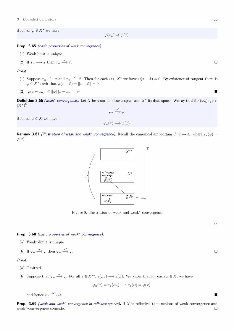
if for all ϕ ∈ X∗ we haveϕ(xn)→ ϕ(x).
Prop. 3.65 (basic properties of weak convergence).
(1) Weak limit is unique.
(2) If xn −→ x then xnw−→ x.
Proof.
(1) Suppose xnw−→ x and xn
w−→ x. Then for each ϕ ∈ X∗ we have ϕ(x− x) = 0. By existence of tangent there isϕ ∈ X∗ such that ϕ(x− x) = ‖x− x‖ = 0.
(2) |ϕ(x− xn)| ≤ ‖ϕ‖|x− xn| X
Definition 3.66 (weak∗-convergence). Let X be a normed linear space and X∗ its dual space. We say that for (ϕn)n∈N ∈(X∗)N
ϕnw∗−→ ϕ,
if for all x ∈ X we haveϕn(x) −→ ϕ(x).
Remark 3.67 (illustration of weak and weak∗ convergence). Recall the canonical embedding J : x 7→ εx where εx(ϕ) =ϕ(x).
X
X∗
X∗∗
w-conv.
w∗-conv.w-conv.
F
x1x2
x
ϕ1ϕ2
J
Figure 8: illustration of weak and weak∗ convergence
//
Prop. 3.68 (basic properties of weak∗ convergence).
(a) Weak∗-limit is unique
(b) If ϕnw−→ ϕ then ϕn
w∗−→ ϕ.
Proof.
(a) Omitted.
(b) Suppose that ϕnw−→ ϕ. For all ε ∈ X∗∗, ε(ϕn) −→ ε(ϕ). We know that for each x ∈ X, we have
ϕn(x) = εx(ϕn) −→ εx(ϕ) = ϕ(x),
and hence ϕnw∗−→ ϕ.
Prop. 3.69 (weak and weak∗ convergence in reflexive spaces). If X is reflexive, then notions of weak convergence andweak∗-convergence coincide.
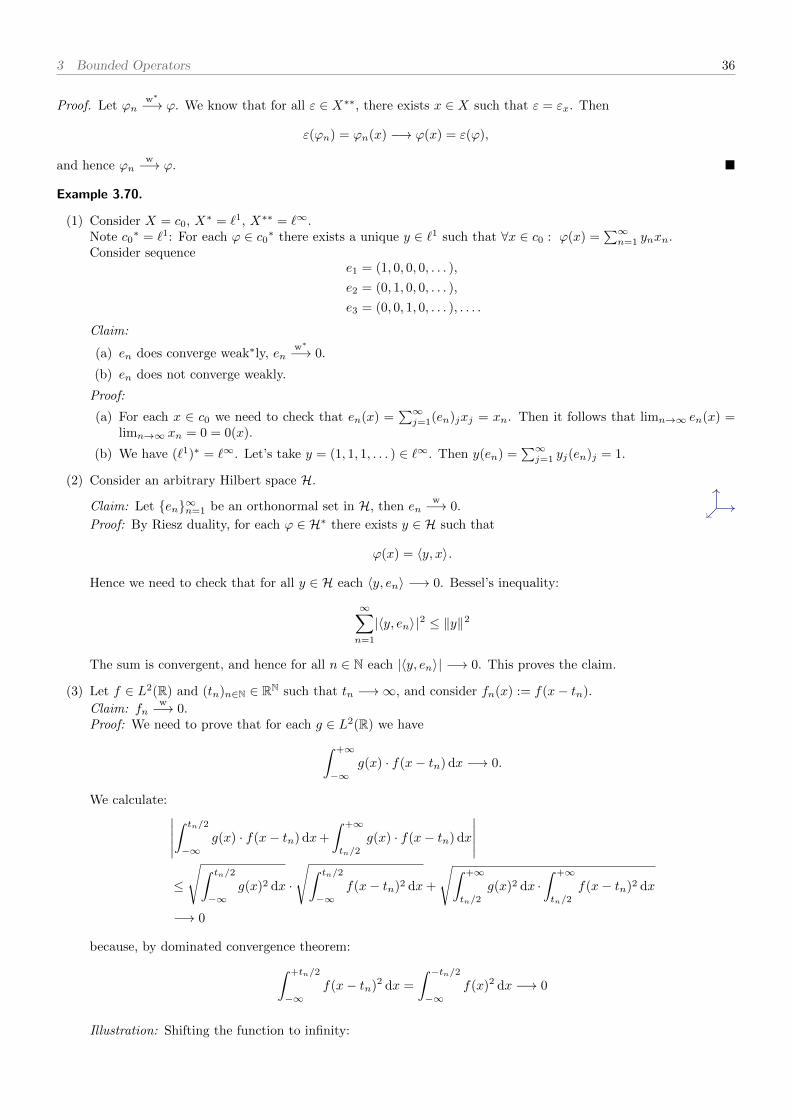
3 Bounded Operators 36
Proof. Let ϕnw∗−→ ϕ. We know that for all ε ∈ X∗∗, there exists x ∈ X such that ε = εx. Then
ε(ϕn) = ϕn(x) −→ ϕ(x) = ε(ϕ),
and hence ϕnw−→ ϕ.
Example 3.70.
(1) Consider X = c0, X∗ = `1, X∗∗ = `∞.Note c0
∗ = `1: For each ϕ ∈ c0∗ there exists a unique y ∈ `1 such that ∀x ∈ c0 : ϕ(x) =∑∞n=1 ynxn.
Consider sequencee1 = (1, 0, 0, 0, . . . ),
e2 = (0, 1, 0, 0, . . . ),
e3 = (0, 0, 1, 0, . . . ), . . . .
Claim:
(a) en does converge weak∗ly, enw∗−→ 0.
(b) en does not converge weakly.
Proof:
(a) For each x ∈ c0 we need to check that en(x) =∑∞j=1(en)jxj = xn. Then it follows that limn→∞ en(x) =
limn→∞ xn = 0 = 0(x).
(b) We have (`1)∗ = `∞. Let’s take y = (1, 1, 1, . . . ) ∈ `∞. Then y(en) =∑∞j=1 yj(en)j = 1.
(2) Consider an arbitrary Hilbert space H.
Claim: Let en∞n=1 be an orthonormal set in H, then enw−→ 0.
Proof: By Riesz duality, for each ϕ ∈ H∗ there exists y ∈ H such that
ϕ(x) = 〈y, x〉.
Hence we need to check that for all y ∈ H each 〈y, en〉 −→ 0. Bessel’s inequality:
∞∑n=1
|〈y, en〉|2 ≤ ‖y‖2
The sum is convergent, and hence for all n ∈ N each |〈y, en〉| −→ 0. This proves the claim.
(3) Let f ∈ L2(R) and (tn)n∈N ∈ RN such that tn −→∞, and consider fn(x) := f(x− tn).
Claim: fnw−→ 0.
Proof: We need to prove that for each g ∈ L2(R) we have∫ +∞
−∞g(x) · f(x− tn) dx −→ 0.
We calculate: ∣∣∣∣∣∫ tn/2
−∞g(x) · f(x− tn) dx+
∫ +∞
tn/2
g(x) · f(x− tn) dx
∣∣∣∣∣≤
√∫ tn/2
−∞g(x)2 dx ·
√∫ tn/2
−∞f(x− tn)2 dx+
√∫ +∞
tn/2
g(x)2 dx ·∫ +∞
tn/2
f(x− tn)2 dx
−→ 0
because, by dominated convergence theorem:∫ +tn/2
−∞f(x− tn)2 dx =
∫ −tn/2−∞
f(x)2 dx −→ 0
Illustration: Shifting the function to infinity:
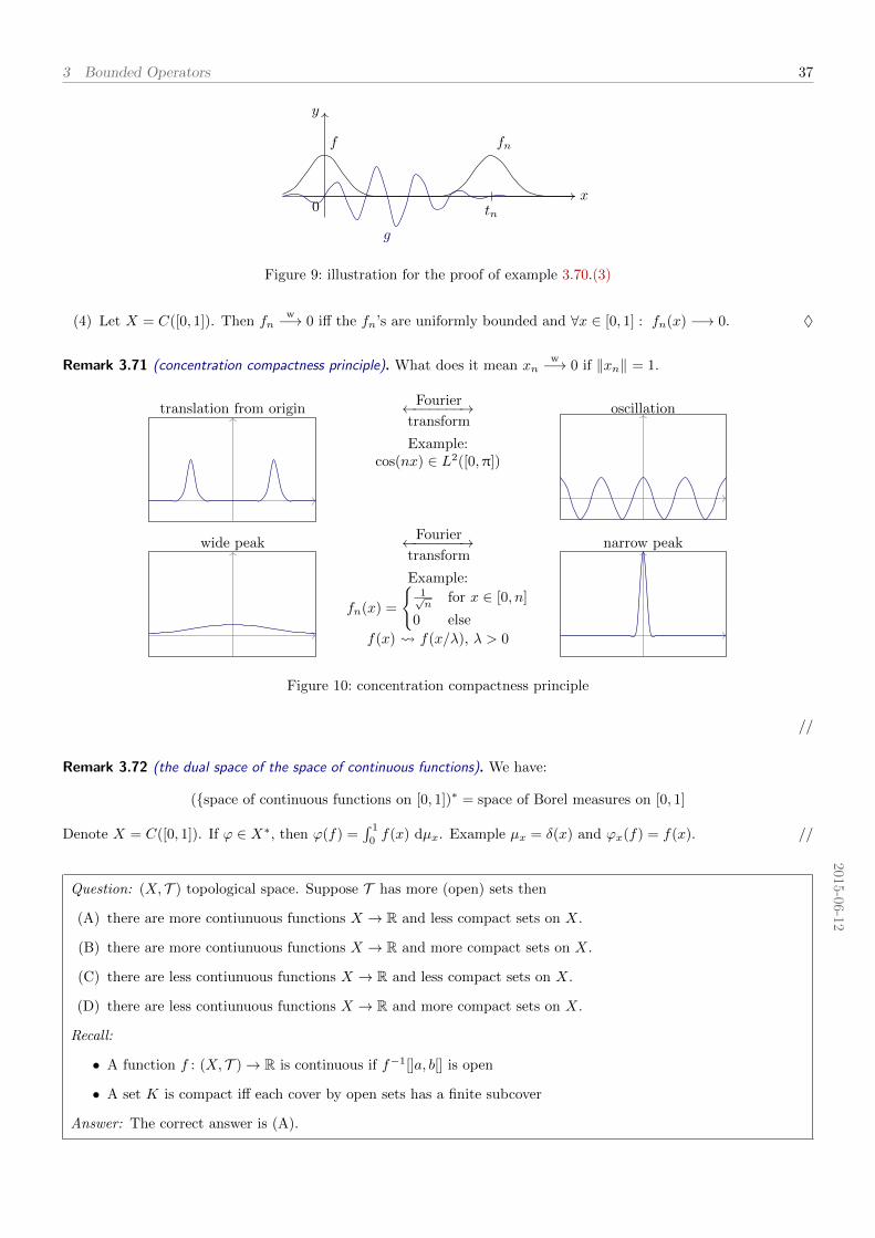
3 Bounded Operators 37
x
y
0 tn
f fn
g
Figure 9: illustration for the proof of example 3.70.(3)
(4) Let X = C([0, 1]). Then fnw−→ 0 iff the fn’s are uniformly bounded and ∀x ∈ [0, 1] : fn(x) −→ 0. ♦
Remark 3.71 (concentration compactness principle). What does it mean xnw−→ 0 if ‖xn‖ = 1.
translation from originFourier←−−−−−−→
transform
Example:cos(nx) ∈ L2([0,π])
oscillation
wide peakFourier←−−−−−−→
transform
Example:
fn(x) =
1√n
for x ∈ [0, n]
0 else
f(x) f(x/λ), λ > 0
narrow peak
Figure 10: concentration compactness principle
//
Remark 3.72 (the dual space of the space of continuous functions). We have:
(space of continuous functions on [0, 1])∗ = space of Borel measures on [0, 1]
Denote X = C([0, 1]). If ϕ ∈ X∗, then ϕ(f) =∫ 1
0f(x) dµx. Example µx = δ(x) and ϕx(f) = f(x). //
2015-06-12
Question: (X, T ) topological space. Suppose T has more (open) sets then
(A) there are more contiunuous functions X → R and less compact sets on X.
(B) there are more contiunuous functions X → R and more compact sets on X.
(C) there are less contiunuous functions X → R and less compact sets on X.
(D) there are less contiunuous functions X → R and more compact sets on X.
Recall:
• A function f : (X, T )→ R is continuous if f−1[]a, b[] is open
• A set K is compact iff each cover by open sets has a finite subcover
Answer: The correct answer is (A).
3 Bounded Operators 38
Prop. 3.73 (continuous functions map compact sets to compact sets). Continuous functions on a compact set achievesits minimum and maximum.
Weak topology:
• (X, T ) is a topological space
• We require that functions in X∗ are continuous. This means that ϕ ∈ X∗, then you neeed that
ϕ−1[]a, b[] open ⇔ x ∈ X | a < ϕ(x) < b open.
Definition 3.74 (weak topology). The weak topology is generated by finite intersections and unions of sets
x | a < |ϕ(x)| < b.
A set U is weakly open if for each x ∈ U there exists ϕ1, . . . , ϕn ∈ X∗ and ε > 0 such that
UX := y ∈ X | ∀j = 1, . . . , n : |ϕj(x)− ϕj(y)| < ε ⊆ U .
Prop. 3.75 (convergence in weak topology = weak convergence). A sequence (xn)n∈N converges to x w.r.t. the weak
topology, if and only if xnw−→ x.
Proof. Proof of “⇒”: For each open set U 3 x there exists n0 such that ∀n ≥ n0 : xn ∈ U . We need to show thatxn
w−→ x, i.e. ∀ϕ ∈ X∗ : ϕ(xn) −→ ϕ(x). Let ε > 0. In particular, Ux = y | |ϕ(x) − ϕ(y)| < ε is open, so thereexists n0 such that for n > n0 we have xn ∈ Ux, hence |ϕ(x0)− ϕ(x)| < ε. We conclude ϕ(xn) −→ ϕ.Proof of “⇐”: See lecture notes.
Remark 3.76. Set of weakly converging sequences does not define weak topology. There are spaces where convergenceweak convergence conincide, but not topology and weak topology. //
Example 3.77 (Schur’s lemma). A sequence (xn)n∈N ∈ `1 converges weakly iff it converges in ‖·‖1-norm. ♦
Lemma 3.78. Let X be an infinite-dimensional normed linear space. And let U be an weakly open set containinig 0.Then there exists a closed non-zero subspace M such that M ⊆ U . In particular U is unbounded.
Proof. There exists ϕ1, . . . , ϕn and ε > 0 such that
U = x | |ϕj(x)| < ε ⊆ U .
We claim that
M =
n⋂j=1
ker(ϕj) ⊆ U
is non-zero (in the sense of M 6= 0) closed subspace. Suppose that M = 0, then the map
L : X → Fn, x 7→ (ϕ1(x), . . . , ϕn(x))
is injective (suppose that Lx = Lx, then L(x − x) = 0, hence (ϕ1(x − x), . . . , ϕn(x − x)) = (0, . . . , 0), contradictionbecause there is no injective map infin.-dim. space→ finite-dim. space).
Remark 3.79. xnw−→ 0, ‖xn‖ = 1 0 //
Definition 3.80 (weak∗ topology). Let X∗ be the dual of X. The weak∗ topology on X∗ is generated by unions andfinite intersections of
ϕ | a < |ϕ(x)| < b, x ∈ X, a, b > 0.
In particular U ⊆ X∗ is weak∗-open if for each ϕ ∈ U exists x1, . . . , xn ∈ X and ε > 0 such that
ψ | |ψ(xj)− ϕ(xj)| < ε ⊆ U .

3 Bounded Operators 39
Prop. 3.81.
(a) If (ϕn)n∈N converges to ϕ in weak∗ topology, then ϕnw∗−→ ϕ.
(b) It is the weakest topology on X∗ in which functions in J [X] are continuous, where J denoted the canonicalembedding.
(c) If X is reflexive, then weak topology on X∗ and weak∗ topology on X∗ conincide.
Remark 3.82.
X
X∗ Fϕ
x X
X∗
X∗∗ FJ [X] εx
εx(ϕ) = ϕ(x)J
Figure 11: Illustration of dual space and canonical embedding.
//
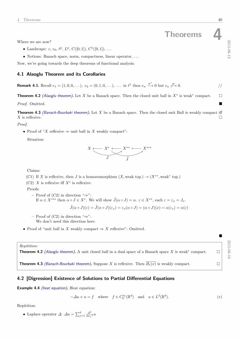
4 Theorems 40
Theorems 4 2015-0
6-1
2
Where we are now?
• Landscape: c, c0, `p, Lp, C([0, 1]), C1([0, 1]), . . .
• Notions: Banach space, norm, compactness, linear operator, . . .
Now, we’re going towards the deep theorems of functional analysis.
4.1 Alaoglu Theorem and its Corollaries
Remark 4.1. Recall e1 = (1, 0, 0, . . . ), e2 = (0, 1, 0, . . . ), . . . in `1 then enw∗−→ 0 but en 6
w−→ 0. //
Theorem 4.2 (Alaoglu theorem). Let X be a Banach space. Then the closed unit ball in X∗ is weak∗ compact.
Proof. Omitted.
Theorem 4.3 (Banach-Bourbaki theorem). Let X be a Banach space. Then the closed unit Ball is weakly compact iffX is reflexive.
Proof.
• Proof of “X reflexive ⇒ unit ball in X weakly compact”:
Situation:
X X∗ X∗∗ X∗∗∗
J J
Claims:
(C1) If X is reflexive, then J is a homoeomorphism (X,weak top.)→ (X∗∗,weak∗ top.)
(C2) X is reflexive iff X∗ is reflexive.
Proofs:
– Proof of (C2) in direction “⇒”:If α ∈ X∗∗∗ then α J ∈ X∗. We will show J(α J) = α. ε ∈ X∗∗, each ε = εx = Jx.
J(α J)(ε) = J(α J)(εx) = εx(α J) = (α J)(x) = α(εx) = α(ε)
– Proof of (C2) in direction “⇒”:We don’t need this direction here.
• Proof of “unit ball in X weakly compact ⇒ X reflexive”: Omitted.
2015-06-16
Repitition:
Theorem 4.2 (Alaoglu theorem). A unit closed ball in a dual space of a Banach space X is weak∗ compact.
Theorem 4.3 (Banach-Bourbaki theorem). Suppose X is reflexive. Then B1(x) is weakly compact.
4.2 [Digression] Existence of Solutions to Partial Differential Equations
Example 4.4 (heat equation). Heat equation:
−∆u+ u = f where f ∈ C∞0 (Rd) and u ∈ L2(Rd). (∗)
Repitition:
• Laplace operator ∆: ∆u =∑dj=1
∂2
∂xj2u

4 Theorems 41
• Gradient operator ∇: ( ∂u∂x1u, . . . , ∂
∂xdu)
Applications:
• This describes heat distribution in a room.
• Similar differential equation for Black-Scholes equation which models prices on the stock market.
Remark:
• We skip technicalities (e.g. we require u ∈ L2(Rd), although the consider ∆u, it would be more correct to useSobolev spaces.)
How can we solve (∗)? ♦
Steps to solve the heat equation
1. Rewrite the equation as minimization problem.
minv∈L2(Rd)
F (v), F : L2(Rd)→ R
Spoiler: Using the Dirichlet principle, we will find:
F (v) :=1
2
∫Rd|∇v(x)|2 dx+
1
2
∫Rdv(x)2 dx−
∫Rdf(x) · v(x) dx
2. Prove that F is bounded from below and weakly lower semi-continuous.
3. Use Banach-Bourbaki to conclude that F achieves its minimum.
1st step to solve the heat equation
Lemma 4.5 (Dirichlet principle). Let
F (u) :=
∫Rd|∇u(x)|2 dx+
1
2
∫Rdu(x)2 dx−
∫Rdf(x) · u(x) dx ,
provided the integrals exist, otherwise F (ω) := ∞. Suppose u is such that F (u) < ∞ and F (u) = infv F (v), then usolves (∗).
Proof. Let g ∈ C∞0 (Rd) and let define F : R→ R, F (λ) := F (u+ λg), then ∀λ ∈ R : F (0) ≤ F (λ). We calculate
F (λ) =
(∫Rd|∇u(x)|2 dx+2λ
∫Rd∇w(x) · ∇g(x) dx+λ2
∫Rd|∇g(x)|2 dx
)+
1
2
(∫Rdu(x)2 dx+2λ
∫Rdw(x) · g(x) dx+λ2
∫Rdg(x)2 dx
)−(∫
Rdf(x) · w(x) dx+λ
∫Rdf(x) · g(x) dx
),
where we have used that
|∇w + λ∇g|2 = 〈∇w + λ∇g,∇w + λ∇g〉 = |∇w|2 + 2λ〈∇w,∇g〉 + λ2|∇g|2.
We note that F is a quadratic form in λ, and because 0 minimizes F , we have F ′(0) = 0.
F ′(0) = 0 ⇔ 2
∫Rd∇w(x) · ∇g(x) dx+
∫Rdu(x) · g(x) dx−
∫Rdf(x) · g(x) dx = 0
(∗)⇔ 2
∫Rd−∆w(x) · g(x) dx+
∫Rdw(x) · g(x) dx−
∫Rd
(−2∆u+ u− f) · g(x) dx
⇔ −∆w(x) + u(x)− f(x) = 0
step at (∗): multivariable version of intgegration by parts = stokes theorem / green identity.Division by factor 2 yields the claim.
3rd step to solve the heat equation
4 Theorems 42
Definition 4.6 (lower semi-continuity). Function F : X → R on a topological space X is lower semi-continuous if for allα ∈ R the set x ∈ X | F (x) > α is open, or equivalently, if xα → x implies F (x) ≤ lim infxα→x F (xα).
Figure 12: Example of lower semi-continuous (left), upper semi-continuous function (middle), and continuous function(right).
Lemma 4.7. A lower semi-continuous functions achieves its minimum on a compact set.
Proof. We assume compactness ⇔ sequential compactness. Let m := infx∈K F (x). Let (xα)α be a sequence inK such that F (xα) → m. Because K is compact, there exists a subsequence xαn → x ∈ K. Then m ≤ F (x) ≤lim infxα→x F (xα) = m, and hence F (x) = m.
Consequence:
Lemma 4.8. Let X be a reflexive Banach space and F : X → R a function. Assume:(i) ∃α ∈ R : x ∈ X | F (x) ≤ α bounded
(ii) F weakly lower semi-continuousThen F achieves its infimum on X.
Proof. The set x ∈ X | F (x) ≤ α is bounded and weakly closed, hence by Banach-Bourbaki it is weakly compact.Then by lemma above, it achieves minimum m on x ∈ X | F (x) ≤ α, and therefore m ≤ α, so it is also a minimumon X.
Lemma 4.9. Let X be a Banach space, then ‖·‖ is weakly lower semi-continuous.
Proof. Exercise.
2nd step to solve the heat equation
Check conditions: Let α > 0.
1
2
∫Rd|∇v(x)|2 dx+
1
2
∫v(x)2 dx−
∫f(x) · v(x) dx ≤ α
LHS =1
2
∫|∇v(x)|2 dx+
1
2
∫v(x)2 dx−
∫f(x) · v(x) dx
CS6=≥ 1
2‖v‖2 −
√∫f(x)2 dx
√∫v(x)2 =
1
2‖v‖2 − ‖f‖‖v‖
Therefore:1
2‖v‖2 − ‖f‖‖v‖ ≤ α
So property (i) follows.
F (v) =1
2
∫‖∇v(x)‖2 dx+
1
2‖v‖2 −
∫f(x) · v(x) dx︸ ︷︷ ︸
weakly continuous
Claim:‖·‖ is weakly continuous
Proof: See lemma above.
Claim: ∫Rd|∇v(x)|2 dx is weakly semi-continuous
4 Theorems 43
Proof: Let vαw−→ v where vα ∈ C∞0 (Rd). I need to compute lim infvα→v
∫Rd |∇vα(x)|2 dx.
∥∥|∇vα|2∥∥2 =
∫Rd|∇vα(x)|2
= supg∈C∞0 (Rd)‖g‖=1
∣∣∣∣∫Rdg(x) · ∇vα(x) dx
∣∣∣∣= supg∈C∞0 (Rd)‖g‖=1
∣∣∣∣−∫Rd∇g(x) · vα(x) dx
∣∣∣∣lim infvα→v
∥∥|∇vα|2∥∥ = lim infvα→v
supg∈C∞0 (Rd)‖g‖=1
∣∣∣∣∫Rd∇g(x) · vα(x) dx
∣∣∣∣≤ supg∈C∞0 (Rd)‖g‖=1
∣∣∣∣∫Rd∇g(x) · vα(x) dx
∣∣∣∣≤ supg∈C∞0 (Rd)‖g‖=1
∣∣∣∣∫Rdg(x) · ∇vα(x) dx
∣∣∣∣≤ supg∈C∞0 (Rd)‖g‖=1
√∫g(x)2 dx
√∫|∇v(x)|2 dx
≤∥∥|∇v|2∥∥
Claim: 2015-0
6-1
9
A function v 7→∫Rd|∇v(x)|2 dx is weakly lower semi-continuous on L2(Rd).
Let vαw−→ v, vα ∈ C∞0 (Rd).
lim infvα→v
√∫Rd|∇vα(x)| dx = lim inf
vα→v‖∇vα‖
= lim infvα→v
supf∈C∞0 ,‖f‖=1
|〈f,∇vα〉|
= lim infvα→v
supf∈C∞0 ,‖f‖=1
|〈∇f, vα〉|
≥ supf∈C∞0 ,‖f‖=1
lim infvα→v
|〈∇f, vα〉|
= supf∈C∞0 ,‖f‖=1
|〈∇f, v〉|
= ‖∇v‖
Where we have used that:
〈∇f, vα〉 =
∫Rd∇f(x) · vα(x) dx =
∑j
∫Rdfj(x) · ∂vα
∂xj(x) dx = −
∑j
∫Rd
∂fj∂xj
(x) · vα(x) dx = −∫Rd∇f(x) · vα(x) dx
Note that:
lim infxα→x
= inf cluster points
infx∈X
supy∈Y
F (x, y) ≥ supy∈Y
infx∈X
F (x, y)
Conclude:∀y ∈ Y : LHS ≥ inf
x∈XF (x, y) ∴ LHS ≥ sup
y∈Yinfx∈X
F (x, y)
4.3 Baire Category Theorem and its Corollaries
2015-06-19
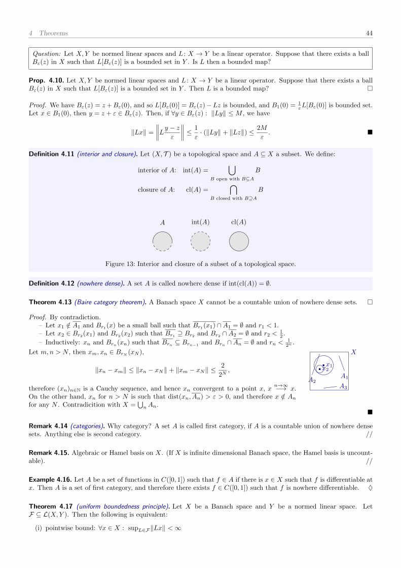
4 Theorems 44
Question: Let X,Y be normed linear spaces and L : X → Y be a linear operator. Suppose that there exists a ballBε(z) in X such that L[Bε(z)] is a bounded set in Y . Is L then a bounded map?
Prop. 4.10. Let X,Y be normed linear spaces and L : X → Y be a linear operator. Suppose that there exists a ballBε(z) in X such that L[Bε(z)] is a bounded set in Y . Then L is a bounded map?
Proof. We have Bε(z) = z+Bε(0), and so L[Bε(0)] = Bε(z)−Lz is bounded, and B1(0) = 1εL[Bε(0)] is bounded set.
Let x ∈ B1(0), then y = z + ε ∈ Bε(z). Then, if ∀y ∈ Bε(z) : ‖Ly‖ ≤M , we have
‖Lx‖ =
∥∥∥∥Ly − zε∥∥∥∥ ≤ 1
ε· (‖Ly‖ + ‖Lz‖) ≤ 2M
ε.
Definition 4.11 (interior and closure). Let (X, T ) be a topological space and A ⊆ X a subset. We define:
interior of A: int(A) =⋃
B open with B⊆A
B
closure of A: cl(A) =⋂
B closed with B⊇A
B
A int(A) cl(A)
Figure 13: Interior and closure of a subset of a topological space.
Definition 4.12 (nowhere dense). A set A is called nowhere dense if int(cl(A)) = ∅.
Theorem 4.13 (Baire category theorem). A Banach space X cannot be a countable union of nowhere dense sets.
Proof. By contradiction.– Let x1 /∈ A1 and Br1(x) be a small ball such that Br1(x1) ∩A1 = ∅ and r1 < 1.– Let x2 ∈ Br2(x1) and Br2(x2) such that Br1 ⊇ Br2 and Br2 ∩A2 = ∅ and r2 <
12 .
– Inductively: xn and Brn(xn) such that Brn ⊆ Brn−1and Brn ∩An = ∅ and rn <
12n .
Let m,n > N , then xm, xn ∈ BrN (xN ),
‖xn − xm‖ ≤ ‖xn − xN‖ + ‖xm − xN‖ ≤2
2N,
therefore (xn)n∈N is a Cauchy sequence, and hence xn convergent to a point x, xn→∞−→ x.
On the other hand, xn for n > N is such that dist(xn, An) > ε > 0, and therefore x /∈ Anfor any N . Contradicition with X =
⋃nAn.
X
x1x2
A1A2A3
Remark 4.14 (categories). Why category? A set A is called first category, if A is a countable union of nowhere densesets. Anything else is second category. //
Remark 4.15. Algebraic or Hamel basis on X. (If X is infinite dimensional Banach space, the Hamel basis is uncount-able). //
Example 4.16. Let A be a set of functions in C([0, 1]) such that f ∈ A if there is x ∈ X such that f is differentiable atx. Then A is a set of first category, and therefore there exists f ∈ C([0, 1]) such that f is nowhere differentiable. ♦
Theorem 4.17 (uniform boundedness principle). Let X be a Banach space and Y be a normed linear space. LetF ⊆ L(X,Y ). Then the following is equivalent:
(i) pointwise bound: ∀x ∈ X : supL∈F‖Lx‖ <∞
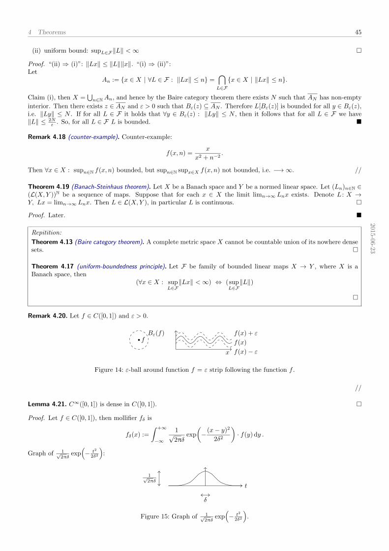
4 Theorems 45
(ii) uniform bound: supL∈F‖L‖ <∞
Proof. “(ii) ⇒ (i)”: ‖Lx‖ ≤ ‖L‖‖x‖. “(i) ⇒ (ii)”:Let
An := x ∈ X | ∀L ∈ F : ‖Lx‖ ≤ n =⋂L∈Fx ∈ X | ‖Lx‖ ≤ n.
Claim (i), then X =⋃n∈NAn, and hence by the Baire category theorem there exists N such that AN has non-empty
interior. Then there exists z ∈ AN and ε > 0 such that Bε(z) ⊆ AN . Therefore L[Bε(z)] is bounded for all y ∈ Bε(z),i.e. ‖Ly‖ ≤ N . If for all L ∈ F it holds that ∀y ∈ Bε(z) : ‖Ly‖ ≤ N , then it follows that for all L ∈ F we have‖L‖ ≤ 2N
ε . So, for all L ∈ F L is bounded.
Remark 4.18 (counter-example). Counter-example:
f(x, n) =x
x2 + n−2.
Then ∀x ∈ X : supn∈N f(x, n) bounded, but supn∈N supx∈X f(x, n) not bounded, i.e. −→∞. //
Theorem 4.19 (Banach-Steinhaus theorem). Let X be a Banach space and Y be a normed linear space. Let (Ln)n∈N ∈(L(X,Y ))N be a sequence of maps. Suppose that for each x ∈ X the limit limn→∞ Lnx exists. Denote L : X →Y, Lx = limn→∞ Lnx. Then L ∈ L(X,Y ), in particular L is continuous.
Proof. Later.
2015-0
6-2
3
Repitition:
Theorem 4.13 (Baire category theorem). A complete metric space X cannot be countable union of its nowhere densesets.
Theorem 4.17 (uniform-boundedness principle). Let F be family of bounded linear maps X → Y , where X is aBanach space, then
(∀x ∈ X : supL∈F‖Lx‖ <∞) ⇔ (sup
L∈F‖L‖)
Remark 4.20. Let f ∈ C([0, 1]) and ε > 0.
fBε(f)
x f(x)− εf(x)
f(x) + ε
Figure 14: ε-ball around function f = ε strip following the function f .
//
Lemma 4.21. C∞([0, 1]) is dense in C([0, 1]).
Proof. Let f ∈ C([0, 1]), then mollifier fδ is
fδ(x) :=
∫ +∞
−∞
1√2πδ
exp
(− (x− y)2
2δ2
)· f(y) dy .
Graph of 1√2πδ
exp(− t2
2δ2
):
t
1√2πδ
δ
Figure 15: Graph of 1√2πδ
exp(− t2
2δ2
).
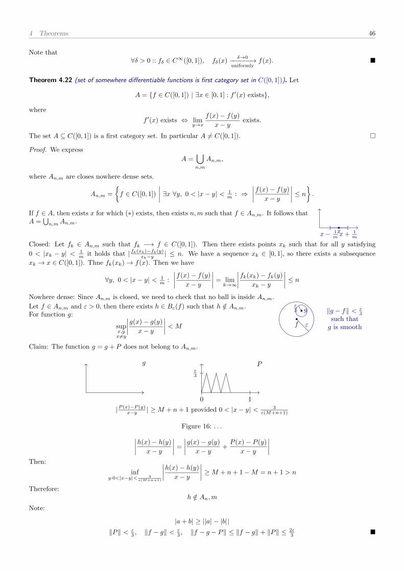
4 Theorems 46
Note that∀δ > 0 :: fδ ∈ C∞([0, 1]), fδ(x)
δ→0−−−−−−→uniformly
f(x).
Theorem 4.22 (set of somewhere differentiable functions is first category set in C([0, 1])). Let
A = f ∈ C([0, 1]) | ∃x ∈ [0, 1] : f ′(x) exists,
where
f ′(x) exists ⇔ limy→x
f(x)− f(y)
x− yexists.
The set A ⊆ C([0, 1]) is a first category set. In particular A 6= C([0, 1]).
Proof. We express
A =⋃n,m
An,m,
where An,m are closes nowhere dense sets.
An,m =
f ∈ C([0, 1])
∣∣∣∣ ∃x ∀y, 0 < |x− y| < 1m : ⇒
∣∣∣∣f(x)− f(y)
x− y
∣∣∣∣ ≤ n .
If f ∈ A, then exists x for which (∗) exists, then exists n,m such that f ∈ An,m. It follows thatA =
⋃n,mAn,m.
x− 1m x+ 1
mx
Closed: Let fk ∈ An,m such that fk −→ f ∈ C([0, 1]). Then there exists points xk such that for all y satisfying
0 < |xk − y| < 1m it holds that | fk(xk)−fk(y)
xk−y | ≤ n. We have a sequence xk ∈ [0, 1], so there exists a subsequence
xk → x ∈ C([0, 1]). Thne fk(xk)→ f(x). Then we have
∀y, 0 < |x− y| < 1m :
∣∣∣∣f(x)− f(y)
x− y
∣∣∣∣ = limk→∞
∣∣∣∣fk(xk)− fk(y)
xk − y
∣∣∣∣ ≤ nNowhere dense: Since An,m is closed, we need to check that no ball is inside An,m.
Let f ∈ An,m and ε > 0, then there exists h ∈ Bε(f) such that h /∈ An,m.For function g:
supx,yx 6=y
∣∣∣∣g(x)− g(y)
x− y
∣∣∣∣ < M
Claim: The function g = g + P does not belong to An,m.
f ε
gε3 ‖g − f‖ < ε
3such thatg is smooth
g P
0 1
ε3
|P (x)−P (y)x−y | ≥M + n+ 1 provided 0 < |x− y| < 3
ε(M+n+1)
Figure 16: . . .∣∣∣∣h(x)− h(y)
x− y
∣∣∣∣ =
∣∣∣∣g(x)− g(y)
x− y+P (x)− P (y)
x− y
∣∣∣∣Then:
infy:0<|x−y|< 3
ε(M+n+1)
∣∣∣∣h(x)− h(y)
x− y
∣∣∣∣ ≥M + n+ 1−M = n+ 1 > n
Therefore:h /∈ An,m
Note:
|a+ b| ≥ ||a| − |b||‖P‖ < ε
3 , ‖f − g‖ < ε3 , ‖f − g − P‖ ≤ ‖f − g‖ + ‖P‖ ≤ 2ε
3
4 Theorems 47
Theorem 4.19 (Banach-Steinhaus theorem). Let X be a Banach space and Ln ∈ L(X,Y ). Suppose that for all x ∈ Xlimn→∞ Lnx exists and denote Lx := limn→∞ Lnx. Then L ∈ L(X,Y ).
Proof. L is linear. L is bounded since Lnx converges for all x. Therefore
∀x ∈ X : supn∈N‖Lnx‖ <∞
uniform boundedness principle
∴ supn∈N‖Ln‖ <∞.
Then let M such that supn∈N‖Ln‖ < M , then we have
‖Lx‖ = limn→∞
‖Lnx‖ ≤ supn∈N‖Lnx‖ ≤ sup
n∈N‖Ln‖‖x‖ ≤M‖x‖.
Prop. 4.23. Suppose that X is a normed linear space and (xn)n∈N ∈ XN is weakly converging. Then (xn)n∈N isbounded.
Theorem 4.24. Let (xn)n∈N be a bounded sequence (supn∈N‖xn‖ ≤ ∞) in a reflexive Banach space. Then (xn)n∈Nhas a weakly converging subsequence.Rephrasing: The closed unit ball in a reflexive Banach space is weakly sequentially compact.
Remark 4.25 (nets). Nets is a generalization of sequences, e.g. they fix the difference “compactness ↔ sequentialcompactness”. //
Prop. 4.26 (closed subspaces of reflexive Banach spaces). Let X be reflexive Banach space and Y a closed subspace.Then:
(a) Y is reflexive Banach space.
(b) If Y is separable, then Y ∗ is separable.
Proof.
(a) Let ϕ ∈ Y ∗ and ϕ ∈ X∗. If ϕ ∈ X∗ then ϕ|Y ∈ Y ∗. If ε ∈ Y ∗∗ then ε ∈ X∗∗, ε(ϕ) = ε(ϕ|Y ). XY
We need to prove that for all ε ∈ Y ∗∗ there exists y ∈ Y such that ε(ϕ) = ϕ(y), i.e. ε = Jy. We know that thereexists x ∈ X such that ε(ϕ) = ϕ(x). Suppose that x /∈ Y , then there exists ϕ ∈ X∗ such that ϕ(x) = 1 andϕ|Y = 0. Then
0 = ε(ϕ|Y ) = ε(ϕ) = ϕ(x) = 1,
contradicition, hence x ∈ Y . We need to prove that for all ϕ ∈ Y ∗ indeed ε(ϕ) = ϕ(y).
(b) Omitted.
2015-06-26
Question: Let L ∈ L(X,Y ) and suppose xnw−→ x; does it imply that Lxn
w−→ Lx?Answer: Yes.Proof: If ϕ ∈ Y ∗.
(L′(ϕ))(xn) = ϕ(L(xn)) −→ ϕ(L(x)) = (L′(ϕ))(x), ‖L‖ = ‖L′‖
X∗ L′ϕ Y ∗ ϕ
X Y
L′
L
Figure 17: Illustration of the dual of a linear map.
Theorem (later): Suppose that L ∈ L(X,Y ) is compact. Then xnw−→ x implies Lxn −→ Lx.
Prop. 4.27 (closed subspaces of reflexive Banach spaces). Let X be a reflexive Banach space and Y a closed subspaceof X. Then Y is a reflexive Banach space.
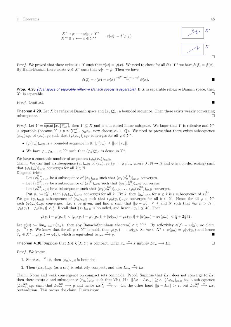
4 Theorems 48
X∗ 3 ϕ −→ ϕ|Y ∈ Y ∗X∗∗ 3 ε ←− ε ∈ Y ∗∗ ε(ϕ) := ε(ϕ|Y )
X∗ϕY ∗
XY
Proof. We proved that there exists x ∈ Y such that ε(ϕ) = ϕ(x). We need to check for all ϕ ∈ Y ∗ we have ε(ϕ) = ϕ(x).By Hahn-Banach there exists ϕ ∈ X∗ such that ϕ|Y = ϕ. Then we have
ε(ϕ) = ε(ϕ) = ϕ(x)x∈Y and ϕ|Y =ϕ
= ϕ(x).
Prop. 4.28 (dual space of separable reflexive Banach spaces is separable). If X is separable reflexive Banach space, thenX∗ is separable.
Proof. Omitted.
Theorem 4.29. Let X be reflexive Banach space and (xn)∞n=1 a bounded sequence. Then there exists weakly convergingsubsequence.
Proof. Let Y = span(xn∞n=1), then Y ⊆ X and it is a closed linear subspace. We know that Y is reflexive and Y ∗
is separable (because Y 3 y '∑Nn=1 αnxn, now choose αn ∈ Q). We need to prove that there exists subsequence
(xnk)k∈N of (xn)n∈N such that (ϕ(xnk))k∈N converges for all ϕ ∈ Y ∗.
• (ϕ(xn))n∈N is a bounded sequence in F, |ϕ(xn)| ≤ ‖ϕ‖‖xn‖.
• We have ϕ1, ϕ2, . . . ∈ Y ∗ such that (ϕn)∞n=1 is dense in Y ∗.
We have a countable number of sequences (ϕn(xn))n∈N.Claim: We can find a subsequence (yn)n∈N of (xn)n∈N (yn = xJ(n), where J : N → N and ϕ is non-decreasing) suchthat (ϕk(yn))n∈N converges for all k ∈ N.Diagonal trick:
– Let (x(1)n )n∈N be a subsequence of (xn)n∈N such that (ϕ1(x
(1)n ))n∈N converges.
– Let (x(2)n )n∈N be a subsequence of (x
(1)n )n∈N such that (ϕ2(x
(2)n ))n∈N converges.
– Let (x(k)n )n∈N be a subsequence such that (ϕ1(x
(k)n ))n∈N, . . . , (ϕk(x
(k)n ))n∈N converges.
– Put yn := x(n)n , then (ϕk(yn))n∈N converges for all k: Fix k, then (yn)n∈N for n ≥ k is a subsequence of x
(k)n .
We got (yn)n∈N subsequence of (xn)n∈N such that (ϕk(yn))n∈N converges for all k ∈ N. Hence for all ϕ ∈ Y ∗
each (ϕ(yn))n∈N converges. Let ε be given, and find k such that ‖ϕ − ϕk‖ ≤ ε3 and N such that ∀m,n > N :
|ϕk(yn)− ϕk(ym)| < ε3 . Recall that (xn)n∈N is bounded, and hence ‖yn‖ ≤M . Then
|ϕ(yn)− ϕ(ym)| < |ϕk(yn)− ϕk(ym)| + |ϕ(yn)− ϕk(yn)| + |ϕ(ym)− ϕk(ym)| < ε3 + 2 ε3M .
Let ε(ϕ) := limn→∞ ϕ(xn). then (by Banach-Steinhaus theorem) ε ∈ Y ∗∗. By reflexivity ε(ϕ) = ϕ(y), we claimyn
w−→ y. We know that for all ϕ ∈ Y ∗ it holds that ϕ(yn) −→ ϕ(y). So ∀ϕ ∈ X∗ : ϕ(yn) = ϕ|Y (yn) and hence∀ϕ ∈ X∗ : ϕ(yn)→ ϕ(y), which is equivalent to yn
w−→ y.
Theorem 4.30. Suppose that L ∈ L(X,Y ) is compact. Then xnw−→ x implies Lxn −→ Lx.
Proof. We know:
1. Since xnw−→ x, then (xn)n∈N is bounded.
2. Then (Lxn)n∈N (as a set) is relatively compact, and also Lxnw−→ Lx.
Claim: Norm and weak convergence on compact sets conincide. Proof: Suppose that Lxn does not converge to Lx,then there exists ε and subsequence (xnk)k∈N such that ∀k ∈ N : ‖Lx − Lxnk‖ ≥ ε. (Lxnk)k∈N has a subsequence
(Lx(2)nk )k∈N such that Lx
(2)nk −→ y and hence Lx
(2)nk
w−→ y. On the other hand ‖y − Lx‖ > ε, but Lx(2)nk
w−→ Lx,contradition. This proves the claim. Illustration:
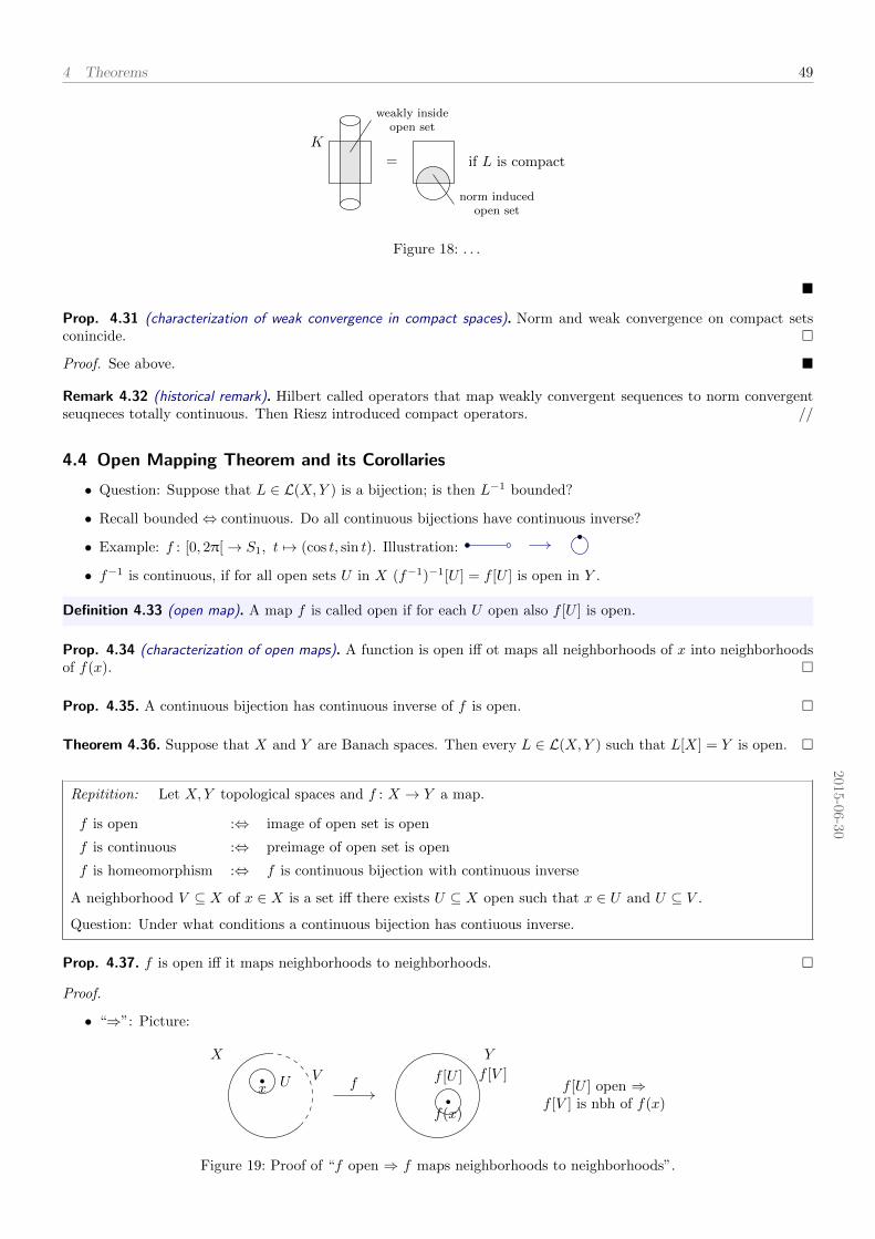
4 Theorems 49
K
weakly insideopen set
norm inducedopen set
= if L is compact
Figure 18: . . .
Prop. 4.31 (characterization of weak convergence in compact spaces). Norm and weak convergence on compact setsconincide.
Proof. See above.
Remark 4.32 (historical remark). Hilbert called operators that map weakly convergent sequences to norm convergentseuqneces totally continuous. Then Riesz introduced compact operators. //
4.4 Open Mapping Theorem and its Corollaries
• Question: Suppose that L ∈ L(X,Y ) is a bijection; is then L−1 bounded?
• Recall bounded⇔ continuous. Do all continuous bijections have continuous inverse?
• Example: f : [0, 2π[→ S1, t 7→ (cos t, sin t). Illustration:
• f−1 is continuous, if for all open sets U in X (f−1)−1[U ] = f [U ] is open in Y .
Definition 4.33 (open map). A map f is called open if for each U open also f [U ] is open.
Prop. 4.34 (characterization of open maps). A function is open iff ot maps all neighborhoods of x into neighborhoodsof f(x).
Prop. 4.35. A continuous bijection has continuous inverse of f is open.
Theorem 4.36. Suppose that X and Y are Banach spaces. Then every L ∈ L(X,Y ) such that L[X] = Y is open.
2015-06-30
Repitition: Let X,Y topological spaces and f : X → Y a map.
f is open :⇔ image of open set is open
f is continuous :⇔ preimage of open set is open
f is homeomorphism :⇔ f is continuous bijection with continuous inverse
A neighborhood V ⊆ X of x ∈ X is a set iff there exists U ⊆ X open such that x ∈ U and U ⊆ V .
Question: Under what conditions a continuous bijection has contiuous inverse.
Prop. 4.37. f is open iff it maps neighborhoods to neighborhoods.
Proof.
• “⇒”: Picture:
X
Vx U
Y
f [V ]
f(x)
f [U ]f f [U ] open ⇒f [V ] is nbh of f(x)
Figure 19: Proof of “f open ⇒ f maps neighborhoods to neighborhoods”.
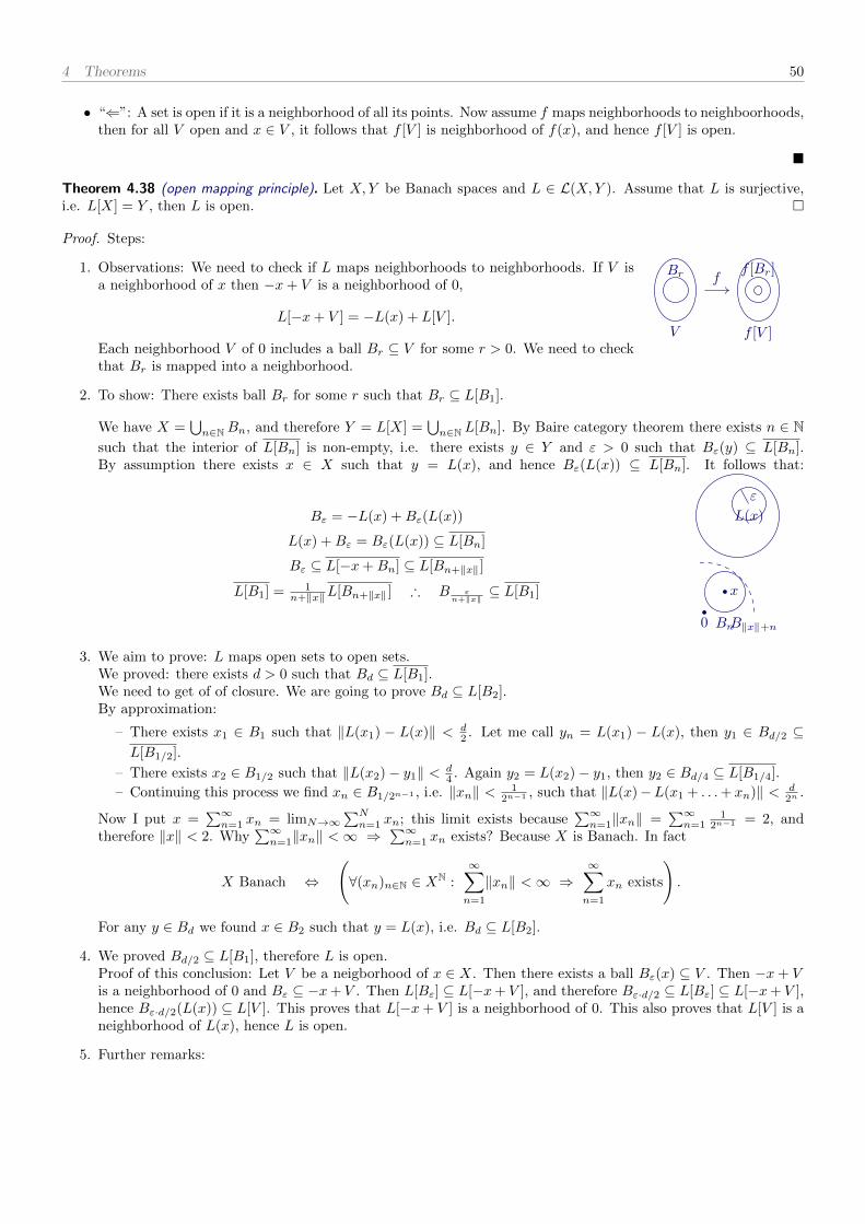
4 Theorems 50
• “⇐”: A set is open if it is a neighborhood of all its points. Now assume f maps neighborhoods to neighboorhoods,then for all V open and x ∈ V , it follows that f [V ] is neighborhood of f(x), and hence f [V ] is open.
Theorem 4.38 (open mapping principle). Let X,Y be Banach spaces and L ∈ L(X,Y ). Assume that L is surjective,i.e. L[X] = Y , then L is open.
Proof. Steps:
1. Observations: We need to check if L maps neighborhoods to neighborhoods. If V isa neighborhood of x then −x+ V is a neighborhood of 0,
L[−x+ V ] = −L(x) + L[V ].
Each neighborhood V of 0 includes a ball Br ⊆ V for some r > 0. We need to checkthat Br is mapped into a neighborhood.
V
Br
f [V ]
f [Br]f
2. To show: There exists ball Br for some r such that Br ⊆ L[B1].
We have X =⋃n∈NBn, and therefore Y = L[X] =
⋃n∈N L[Bn]. By Baire category theorem there exists n ∈ N
such that the interior of L[Bn] is non-empty, i.e. there exists y ∈ Y and ε > 0 such that Bε(y) ⊆ L[Bn].By assumption there exists x ∈ X such that y = L(x), and hence Bε(L(x)) ⊆ L[Bn]. It follows that:
Bε = −L(x) +Bε(L(x))
L(x) +Bε = Bε(L(x)) ⊆ L[Bn]
Bε ⊆ L[−x+Bn] ⊆ L[Bn+‖x‖ ]
L[B1] = 1n+‖x‖L[Bn+‖x‖ ] ∴ B ε
n+‖x‖⊆ L[B1]
L(x)
ε
0
x
BnB‖x‖+n
3. We aim to prove: L maps open sets to open sets.We proved: there exists d > 0 such that Bd ⊆ L[B1].We need to get of of closure. We are going to prove Bd ⊆ L[B2].By approximation:
– There exists x1 ∈ B1 such that ‖L(x1) − L(x)‖ < d2 . Let me call yn = L(x1) − L(x), then y1 ∈ Bd/2 ⊆
L[B1/2].
– There exists x2 ∈ B1/2 such that ‖L(x2)− y1‖ < d4 . Again y2 = L(x2)− y1, then y2 ∈ Bd/4 ⊆ L[B1/4].
– Continuing this process we find xn ∈ B1/2n−1 , i.e. ‖xn‖ < 12n−1 , such that ‖L(x)−L(x1 + . . .+ xn)‖ < d
2n .
Now I put x =∑∞n=1 xn = limN→∞
∑Nn=1 xn; this limit exists because
∑∞n=1‖xn‖ =
∑∞n=1
12n−1 = 2, and
therefore ‖x‖ < 2. Why∑∞n=1‖xn‖ <∞ ⇒
∑∞n=1 xn exists? Because X is Banach. In fact
X Banach ⇔
(∀(xn)n∈N ∈ XN :
∞∑n=1
‖xn‖ <∞ ⇒∞∑n=1
xn exists
).
For any y ∈ Bd we found x ∈ B2 such that y = L(x), i.e. Bd ⊆ L[B2].
4. We proved Bd/2 ⊆ L[B1], therefore L is open.Proof of this conclusion: Let V be a neigborhood of x ∈ X. Then there exists a ball Bε(x) ⊆ V . Then −x+ Vis a neighborhood of 0 and Bε ⊆ −x+ V . Then L[Bε] ⊆ L[−x+ V ], and therefore Bε·d/2 ⊆ L[Bε] ⊆ L[−x+ V ],hence Bε·d/2(L(x)) ⊆ L[V ]. This proves that L[−x+ V ] is a neighborhood of 0. This also proves that L[V ] is aneighborhood of L(x), hence L is open.
5. Further remarks:
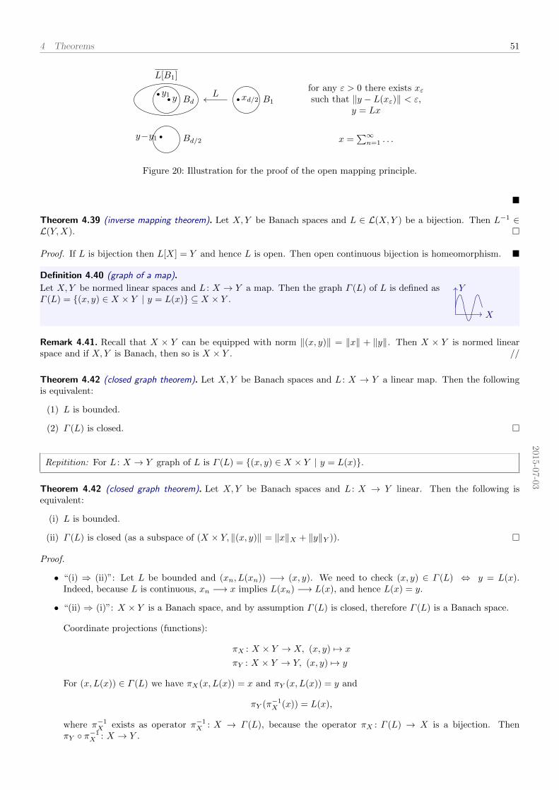
4 Theorems 51
y1 y Bd
L[B1]
xd/2 B1
y−y1 Bd/2
Lfor any ε > 0 there exists xεsuch that ‖y − L(xε)‖ < ε,
y = Lx
x =∑∞n=1 . . .
Figure 20: Illustration for the proof of the open mapping principle.
Theorem 4.39 (inverse mapping theorem). Let X,Y be Banach spaces and L ∈ L(X,Y ) be a bijection. Then L−1 ∈L(Y,X).
Proof. If L is bijection then L[X] = Y and hence L is open. Then open continuous bijection is homeomorphism.
Definition 4.40 (graph of a map).
Let X,Y be normed linear spaces and L : X → Y a map. Then the graph Γ (L) of L is defined asΓ (L) = (x, y) ∈ X × Y | y = L(x) ⊆ X × Y .
X
Y
Remark 4.41. Recall that X × Y can be equipped with norm ‖(x, y)‖ = ‖x‖ + ‖y‖. Then X × Y is normed linearspace and if X,Y is Banach, then so is X × Y . //
Theorem 4.42 (closed graph theorem). Let X,Y be Banach spaces and L : X → Y a linear map. Then the followingis equivalent:
(1) L is bounded.
(2) Γ (L) is closed.
2015-0
7-03
Repitition: For L : X → Y graph of L is Γ (L) = (x, y) ∈ X × Y | y = L(x).
Theorem 4.42 (closed graph theorem). Let X,Y be Banach spaces and L : X → Y linear. Then the following isequivalent:
(i) L is bounded.
(ii) Γ (L) is closed (as a subspace of (X × Y, ‖(x, y)‖ = ‖x‖X + ‖y‖Y )).
Proof.
• “(i) ⇒ (ii)”: Let L be bounded and (xn, L(xn)) −→ (x, y). We need to check (x, y) ∈ Γ (L) ⇔ y = L(x).Indeed, because L is continuous, xn −→ x implies L(xn) −→ L(x), and hence L(x) = y.
• “(ii) ⇒ (i)”: X × Y is a Banach space, and by assumption Γ (L) is closed, therefore Γ (L) is a Banach space.
Coordinate projections (functions):
πX : X × Y → X, (x, y) 7→ x
πY : X × Y → Y, (x, y) 7→ y
For (x, L(x)) ∈ Γ (L) we have πX(x, L(x)) = x and πY (x, L(x)) = y and
πY (π−1X (x)) = L(x),
where π−1X exists as operator π−1
X : X → Γ (L), because the operator πX : Γ (L) → X is a bijection. ThenπY π−1
X : X → Y .
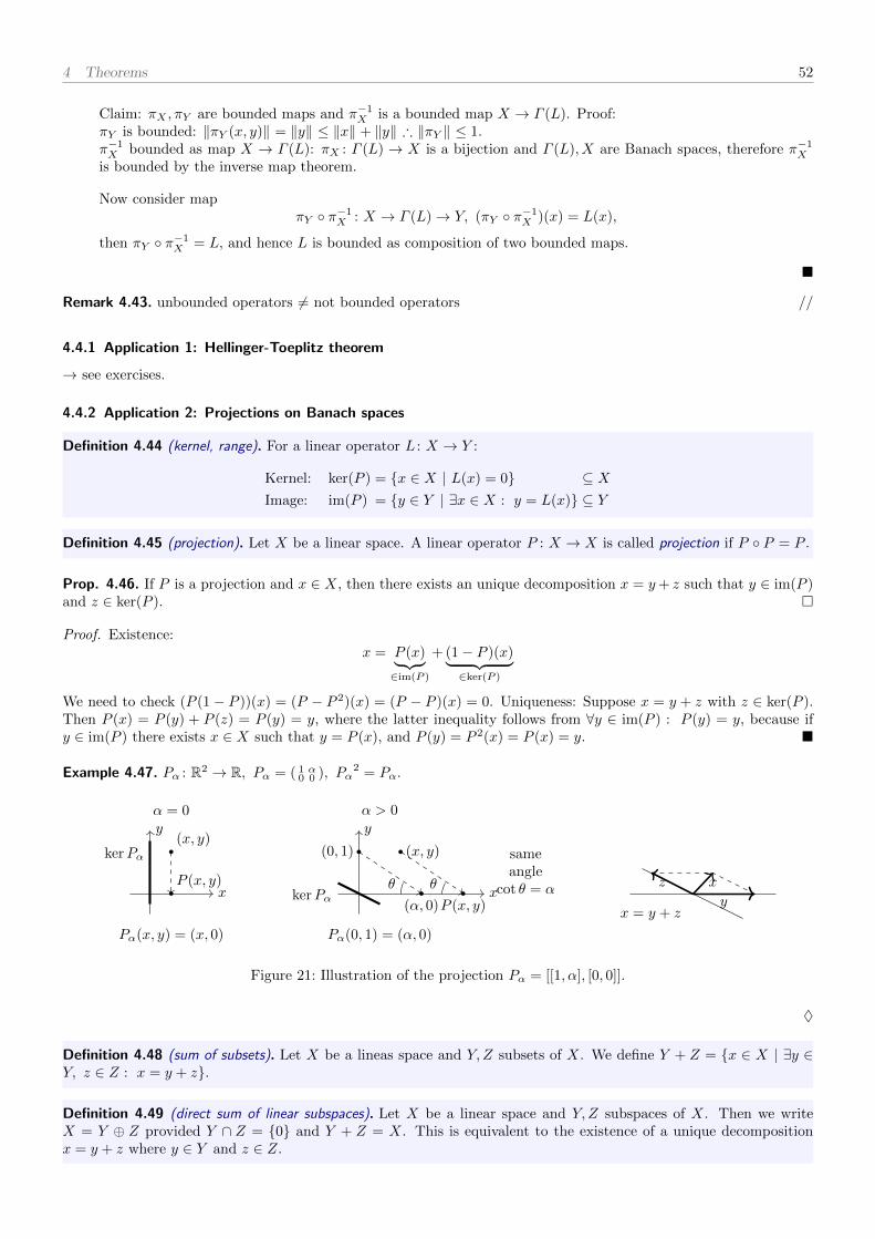
4 Theorems 52
Claim: πX , πY are bounded maps and π−1X is a bounded map X → Γ (L). Proof:
πY is bounded: ‖πY (x, y)‖ = ‖y‖ ≤ ‖x‖ + ‖y‖ ∴ ‖πY ‖ ≤ 1.π−1X bounded as map X → Γ (L): πX : Γ (L) → X is a bijection and Γ (L), X are Banach spaces, therefore π−1
X
is bounded by the inverse map theorem.
Now consider mapπY π−1
X : X → Γ (L)→ Y, (πY π−1X )(x) = L(x),
then πY π−1X = L, and hence L is bounded as composition of two bounded maps.
Remark 4.43. unbounded operators 6= not bounded operators //
4.4.1 Application 1: Hellinger-Toeplitz theorem
→ see exercises.
4.4.2 Application 2: Projections on Banach spaces
Definition 4.44 (kernel, range). For a linear operator L : X → Y :
Kernel: ker(P ) = x ∈ X | L(x) = 0 ⊆ XImage: im(P ) = y ∈ Y | ∃x ∈ X : y = L(x) ⊆ Y
Definition 4.45 (projection). Let X be a linear space. A linear operator P : X → X is called projection if P P = P .
Prop. 4.46. If P is a projection and x ∈ X, then there exists an unique decomposition x = y+ z such that y ∈ im(P )and z ∈ ker(P ).
Proof. Existence:x = P (x)︸ ︷︷ ︸
∈im(P )
+ (1− P )(x)︸ ︷︷ ︸∈ker(P )
We need to check (P (1− P ))(x) = (P − P 2)(x) = (P − P )(x) = 0. Uniqueness: Suppose x = y + z with z ∈ ker(P ).Then P (x) = P (y) + P (z) = P (y) = y, where the latter inequality follows from ∀y ∈ im(P ) : P (y) = y, because ify ∈ im(P ) there exists x ∈ X such that y = P (x), and P (y) = P 2(x) = P (x) = y.
Example 4.47. Pα : R2 → R, Pα = ( 1 α0 0 ), Pα
2 = Pα.
α = 0
Pα(x, y) = (x, 0)
x
y(x, y)
P (x, y)
kerPα
α > 0
Pα(0, 1) = (α, 0)
x
y
(0, 1)
(α, 0)
(x, y)
P (x, y)
θ θ
sameangle
cot θ = αkerPα y
z x
x = y + z
Figure 21: Illustration of the projection Pα = [[1, α], [0, 0]].
♦
Definition 4.48 (sum of subsets). Let X be a lineas space and Y,Z subsets of X. We define Y + Z = x ∈ X | ∃y ∈Y, z ∈ Z : x = y + z.
Definition 4.49 (direct sum of linear subspaces). Let X be a linear space and Y,Z subspaces of X. Then we writeX = Y ⊕ Z provided Y ∩ Z = 0 and Y + Z = X. This is equivalent to the existence of a unique decompositionx = y + z where y ∈ Y and z ∈ Z.
4 Theorems 53
Remark 4.50 (algebraic ↔ geometric). Given P we define Y = im(P ) and Z = ker(P ). Given X = Y ⊕ Z, we candefine P : X → X given by P (x) = y given x = y + z. Claim: P is projection. //
Question: If X is normed linear space, would the decomposition X = Y ⊕ Z contiuous? (x = y + z)Answer: This is equivalent to P being bounded.Proof: y = P (x); x = P (x) + (1− P )(x); xn → x ⇒ yn → y.
Lemma 4.51. Let X be a normed linear space and L a bounded map on X. Then ker(L) is closed linear subspace.
Proof. Let (xn)n∈N ∈ (ker(L))N be such that xnn→∞−→ x. By continuity of L we have 0 = L(xn)
n→∞−→ L(x), thereforeL(x) = 0, i.e. x ∈ ker(L).
Theorem 4.52. Let X be a Banach space and Y,Z two subspaces such that X = Y ⊕ Z. Then the following isequivalent:
(i) Associated projection P is bounded.
(ii) Y,Z are closed.
Proof.
• “(i) ⇒ (ii)”: Put Y = im(P ) and Z = ker(P ). Then Z is closed by the lemma above, and Y is closed becauseY = ker(1− P ).Let’s proof Y = ker(1 − P ): “⊆”: If y ∈ im(P ) then y ∈ ker(1 − P ), because y = P (x) implies (1 − P )(y) =(1− P )(P (x)) = (P − P )(x) = 0. “⊇”: Let y ∈ ker(1− P ), then (1− P )(y) = 0, hence y = P (y).
• “(ii) ⇒ (i)”: Suppose that Y, Z are closed. We want to show that P (x) = y (x = y + z) is bounded.
Γ (P ) = (x, y) ∈ X × Y | x = y + z
1st version of the proof:Γ (P ) closed ⇔ xn = yn+zn and (xn, yn)→ (x, y) then y ∈ Y . In particular xn → x and yn → y, and thereforezn → z. We conclude x = y + z.2nd version of the proof:Γ (P ) closed ⇔ xn = yn + zn. If (xn, yn) → (x, y) then (x, y) ∈ Γ (P ). From xn → x and yn → y it followsthat zn → z such that x = y + z. Since Y and Z are closed, yn → y implies y ∈ Y and zn → z implies z ∈ Z,together this implies (x, y) ∈ Γ (P ). By closed graph theorem, this implies that P is a bounded operator.
2015-07-07
Repitition: Banach space X = Y ⊕ Z ↔ P projection with Y = ker(P ), Z = im(P )Claim: P bounded ⇔ Y,Z closed
Example 4.53.
(1) Consider c = (xn)n∈N sequence | limn→∞ xn exists, in particular c0 ⊆ c.Let Z be a subspace generated by z = (1, 1, 1, . . . ). Then c = c0 ⊕ Z.
∀x ∈ c : x = x0︸︷︷︸∈c0
+ α︸︷︷︸∈R
·z
Px = z( limn→∞
xn︸ ︷︷ ︸=α
)
(2) Let (X,Σ, µ) probability space µ(X) = 1. Random variable is measureable function f : X → R. For f ∈ L1(X)the expectation value E[F ] of f is
E[f ] =
∫X
f dµ .
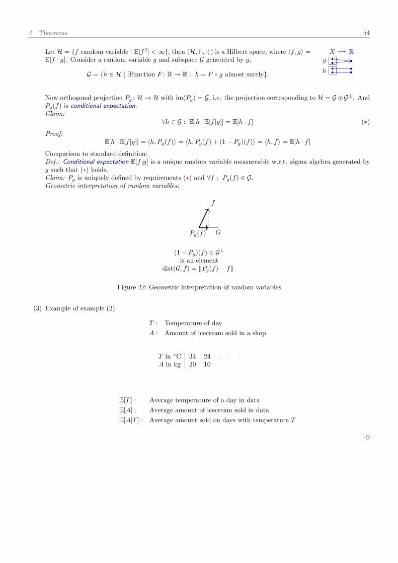
4 Theorems 54
Let H = f random variable | E[f2] <∞, then (H, 〈·, ·〉) is a Hilbert space, where 〈f, g〉 =E[f · g]. Consider a random variable g and subspace G generated by g,
G = h ∈ H | ∃function F : R→ R : h = F g almost surely.
X Rg
h
Now orthogonal projection Pg : H → H with im(Pg) = G, i.e. the projection corresponding to H = G ⊕G⊥. AndPg(f) is conditional expectation.Claim:
∀h ∈ G : E[h · E[f |g]] = E[h · f ] (∗)
Proof:E[h · E[f |g]] = 〈h, Pg(f)〉 = 〈h, Pg(f) + (1− Pg)(f)〉 = 〈h, f〉 = E[h · f ]
Comparison to standard definition:Def.: Conditional expectation E[f |g] is a unique random variable measureable w.r.t. sigma algebra generated byg such that (∗) holds.Claim: Pg is uniquely defined by requirements (∗) and ∀f : Pg(f) ∈ G.Geometric interpretation of random variables:
(1− Pg)(f) ∈ G⊥is an element
dist(G, f) = ‖Pg(f)− f‖.
G
f
Pg(f)
Figure 22: Geometric interpretation of random variables
(3) Example of example (2):
T : Temperature of day
A : Amount of icecream sold in a shop
T in C 34 24 . . .A in kg 20 10
E[T ] : Average temperature of a day in data
E[A] : Average amount of icecream sold in data
E[A|T ] : Average amount sold on days with temperature T
♦
5 Spectral Theory 55
Spectral Theory 55.1 The Spectrum of an Operator
2015-0
7-0
7
Let X complex Banach space, we consider space L(X).
Def./Lemma 5.1 (kernel, image, invertibility). For L ∈ L(X) we have:
kernel of L: ker(L) := x ∈ X | L(x) = 0 ⊆ Ximage of L: im(L) := x ∈ X | ∃y ∈ X : x = L(y) ⊆ Xinvertability of L: L invertible :⇔ ∃L−1 ∈ L(X) : L−1 L = id = L L−1
inverse map theorem: L invertible ⇔ ker(L) = 0 ∧ im(L) = X
Definition 5.2 (spectrum). For L ∈ L(X) we have:
resolvent of L: %(L) := λ ∈ C | L− λid invertible ⊆ Cspectrum of L: σ(L) := λ ∈ C | ker(L− λid) 6= 0 ∨ im(L− λid) 6= X ⊆ Cpoint spectrum of L: σpt(L) := λ ∈ σ(L) | ker(L− λid) 6= 0 = λ ∈ σ(L) | ∃x 6= 0 : L(x) = λ · x ⊆ C
Theorem 5.3 (basic properties of the spectrum).
(i) σ(L) ∩ %(L) = ∅
(ii) σ(L) ∪ %(L) = C
(iii) σ(L) is a compact subset of C
Proof.
(i) X
(ii) By inverse map theorem for each λ either ker(L− λid) 6= 0 or im(L− λid) 6= X or L− λid invertible.
(iii) Little bit work.Claim: %(L) is open subset of C (this implies σ(L) is closed).Proof: Let λ ∈ %(L), then (L− λid)−1 exists by the lemma below. For each λ∥∥∥(L− λid − (L− λid))
∥∥∥ =∣∣∣λ− λ∣∣∣ < 1
‖(L− λid)−1‖,
therefore L− λid is invertible, in particular λ ∈ %(L), and hence %(L) is open.We prove (iii) by proving that Γ (L) is bounded.
Lemma 5.4 (invertiblity is perserved under small perturburations). Let L ∈ L(X) be invertible and S ∈ L(X) such that‖S − L‖ < ‖L−1‖−1, then S is invertible.
Proof. We calculate:S = S − L+ L = L (L−1 (S − L) + 1)
We are going to use the geometric series:
∀x ∈ C, |x| < 1 :1
1 + x=
∞∑n=0
(−1)nxn resp. ∀x ∈ C, |x| < 1 :1
1− x=
∞∑n=0
xn
Observations:
1.∑∞n=0 x
n is absolutely converging (‖xn‖ ≤ ‖x‖n), therefore limN→∞∑Nn=0 x
n exists.
2. (1− x)∑Nn=0 x
n = (1− x) · (1 + x+ x2 + . . .+ xN ) = 1− xN+1 N→∞−→ 1.
To finish the proof observe that ∥∥L−1 (S − L)∥∥ ≤ ∥∥L−1
∥∥ · ‖S − L‖ < 1,
therefore L−1 (S − L) + 1 is invertible and
S−1 = (L−1 (S − L) + 1)−1 L−1.

5 Spectral Theory 56
Prop. 5.5. If |λ| > ‖L‖, then L− λid is invertible, hence σ(L) ⊆ B‖L‖ .
Proof. L− λid = λ(Lλ − id), and since ‖Lλ ‖ < 1, then
(L− λid)−1Lemmaabove= − 1
λ
∞∑n=0
(L
λ
)n= −
∞∑n=0
λ−n−1Ln.0‖L‖
σ(L)
%(L)
2015-0
7-1
0
Repitition: X complex Banach space, L ∈ L(X).– Spectrum σ(L) = λ ∈ C | ker(L− λ) 6= 0 ∨ im(L− λ) 6= 0– Resolvent %(L) = λ ∈ C | L− λ invertible– Claim: σ(L) is a compact subset of λ ∈ C | |λ| ≤ ‖L‖
5.2 Applications of Spectral Theory
5.2.1 Overview
Overview:
(A) functional calculus
(B) diagonalization
(C) transformation to canonical form
5.2.2 (A) Functional Calculus
Given function f : C→ C, the task is to complete f(L).Example: For f(t) = t2 we have f(L) = L2.
5.2.3 (B) Diagonalization
Little bit of linear algebra. Consider X = Cd (finite-dimensional) and L ∈ L(X).
Definition 5.6 (eigenvalues and eigenvectors in finite dimensions). Let λ ∈ C and xλ ∈ X \0. If xλ solves the equationL(xλ) = λ · xλ, then xλ eigenvector and λ eigenvalue.
Remark 5.7. If ker(L− λ) 6= 0, then λ ∈ σpt(L), i.e. λ belongs to the point spectrum of L. //
Prop. 5.8 (Fredholm alternative). In finite dimensions ker(L) 6= 0⇔ im(L) 6= X.
Proof. L(x) = y is solveable iff det(L) 6= 0.
Corollary 5.9. σ(L) = set of all eigenvalues of L
5.2.4 (A) Functional Calculus
Theorem 5.10. Assume that L has d linearly independent eigenvectors (xn)n=1,...,d associated to eigenvalues (λn)n=1,...,d.Then there exists invertible matrix V such thatλ1 0
. . .
0 λd
= V LV −1.
If L = L∗, then V −1 = V ∗ (unitary). In that case:
f
λ1 0
. . .
0 λd
=
f(λ1) 0. . .
0 f(λd)
and f(V LV −1) = V f(L)V −1
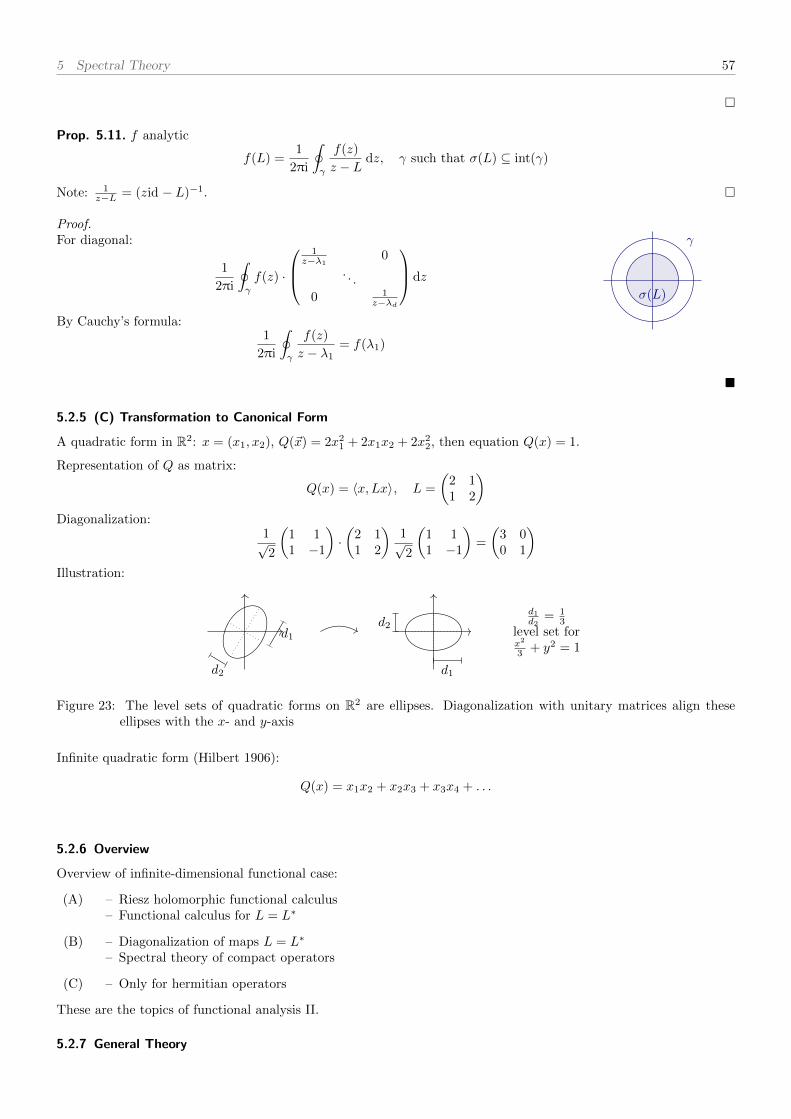
5 Spectral Theory 57
Prop. 5.11. f analytic
f(L) =1
2πi
∮γ
f(z)
z − Ldz, γ such that σ(L) ⊆ int(γ)
Note: 1z−L = (zid − L)−1.
Proof.For diagonal:
1
2πi
∮γ
f(z) ·
1
z−λ10
. . .
0 1z−λd
dz
By Cauchy’s formula:1
2πi
∮γ
f(z)
z − λ1= f(λ1)
σ(L)
γ
5.2.5 (C) Transformation to Canonical Form
A quadratic form in R2: x = (x1, x2), Q(~x) = 2x21 + 2x1x2 + 2x2
2, then equation Q(x) = 1.
Representation of Q as matrix:
Q(x) = 〈x, Lx〉, L =
(2 11 2
)Diagonalization:
1√2
(1 11 −1
)·(
2 11 2
)1√2
(1 11 −1
)=
(3 00 1
)Illustration:
d1
d2 d1
d2
d1d2
= 13
level set forx2
3 + y2 = 1
Figure 23: The level sets of quadratic forms on R2 are ellipses. Diagonalization with unitary matrices align theseellipses with the x- and y-axis
Infinite quadratic form (Hilbert 1906):
Q(x) = x1x2 + x2x3 + x3x4 + . . .
5.2.6 Overview
Overview of infinite-dimensional functional case:
(A) – Riesz holomorphic functional calculus– Functional calculus for L = L∗
(B) – Diagonalization of maps L = L∗
– Spectral theory of compact operators
(C) – Only for hermitian operators
These are the topics of functional analysis II.
5.2.7 General Theory

5 Spectral Theory 58
Definition 5.12 (dual operator). Recall: X, X∗. For L ∈ L(X) define the dual L′ ∈ L(X∗) by
(L′(ϕ))(x) = ϕ(L(x)), ϕ ∈ X∗, x ∈ X.
Definition 5.13 (annihilator). Let M be subspace of X and N subspace of X∗.
annihilator of M ⊆ X: M⊥ := ϕ ∈ X∗ | ∀x ∈M : ϕ(x) = 0 i.e. ϕ|M = 0 ⊆ X∗
annihilator of N ⊆ X∗: ⊥N := x ∈ X | ∀ϕ ∈ N : ϕ(x) = 0 i.e. ϕ|N = 0 ⊆ X
Lemma 5.14. ⊥(M⊥) = M .
Lemma 5.15. Let L ∈ L(X) and denote the dual of L by L′ ∈ L(X∗). Then:
(i) (im(L))⊥ = ker(L′)
(ii) ker(L) = ⊥(im(L′))
(iii) im(L) = ⊥(ker(L′))
Proof.
(i) Let ϕ ∈ (im(L))⊥, this means ∀x ∈ X : ϕ(L(x)) = 0. Because 0 = ϕ(L(x)) = (L′(ϕ))(x) it follows thatL′(ϕ) = 0, i.e. ϕ ∈ ker(L′. Let ϕ ∈ ker(L′), then 0 = (L′(ϕ))(x) = ϕ(L(x)), and therefore ∀y ∈ im(L) : ϕ(y) = 0,i.e. ϕ ∈ (im(L))⊥.
(ii) Do it yourself.
(iii) Taking (i) and applying ⊥(·) implies (iii).
5.2.8 (B) Diagonalization
Relevance of L′ for diagonalization: We consider d× d matrix L.
Prop. 5.16. Every eigenvalue of L is also an eigenvalue of L′, i.e. ∀λ ∈ C : λ ∈ σ(L) ⇒ λ ∈ σ(L′).
Proof. Let λ be an eigenvalue of L, then
ker(L− λ) 6= 0 ∴ im(L− λ) 6= X ∴ ker(L′ − λ) 6= 0,
hence λ is an eigenvalue of L′.
Prop. 5.17. Let λ be an eigenvalue associated to xλ. Let further λ be an eigenvalue xλ. If λ 6= λ, then xλ ∈im(L− λ).
Proof. If λ ∈ σ(L), then λ ∈ σ(L′), hence ∀ϕλ ∈ X∗ : L′(ϕλ) = λ · ϕλ. By (iii), for any x ∈ im(L − λ) we haveϕλ(x) = 0.
(L− λ)1
λ− λxλ =
1
λ− λ(λ− λ)xλxλ = xλ
By ϕλ(x) = 0 it follows that ∀λ 6= λ : ϕλ(xλ) = 0.
Theorem 5.18. Suppose again that L has d distinct eigenvalues with eigenvectors xλ, then L′ has the same eigenvaluesto which we can choose ϕλ with L′(ϕλ) = λ · ϕλ such that
L(x) =∑
λ∈σ(L)
λ︸︷︷︸=:righteigen-value
· xλ · ϕλ(x)︸ ︷︷ ︸=:lefteigen-value
.
Why this is diagonalization? It holds that ϕλ(xλ′) = δλ,λ′ . If x =∑λ∈σ(L) cλxλ, then
L(x) =∑
λ∈σ(L)
λxλϕλ(x) =∑
λ∈σ(L)
λxλcλ,
where cλ ∈ C.
5 Spectral Theory 59
Proof. We know that there exist ϕλ with ϕλ(xϕ) if λ 6= λ. Since ϕλ is nonzero, then we can find ϕλ = #λϕλ suchthat ϕλ(xλ) = 1 where #λ = 1
ϕλ(xλ) . Therefore we have sets ϕλλ∈σ(L) (basis of X∗) and xλλ∈σ(L) (basis of X).
ϕλ(xλ) = δλ,λ. I need to check L(xλ) =∑λ∈σ(L) λxλϕλ(xλ) = λxλ.
5.3 Spectral Theory of Compact Operators
5.3.1 Introduction
2015-0
7-1
4
Consider a Hilbert space L2(X,µ) =: H. Then for f ∈ H
‖f‖2 =
∫X
|f(x)|2 dµ(x) <∞.
Given φ ∈ L∞(X,µ), then we define Lφ ∈ L(H) by
(Lφf)(x) = φ(x) · f(x).
This map has very nice properites:
(a) Lφ is bounded:
‖Lφf‖22 =
∫X
|φ(x) · f(x)|2 dµ(x) ≤ ‖φ‖2∞ · ‖f‖2
2.
(b) The spectrum σ(Lφ) is the essential image of φ, i.e.
λ ∈ σ(Lφ) ⇔ ∀ε > 0 : µ(x ∈ X | |φ(x)− λ| > ε) > 0.
Why? z ∈ %(Lφ) iff (Lφ − zid)−1 exists. If (Lφ − zid)−1, then L(φ−z)−1(Lφ − zid)(f) = (φ− z)−1(φ− z)f = f ,
and z ∈ %(Lφ) iff 1φ−z ∈ L
∞(X,µ).
(c) λ is in the point specturm σpt(Lφ) if µ(x ∈ X | φ(x) = λ) > 0:
λ ∈ σpt(Lφ) ⇔ ∃fλ ∈ L2(X,µ) \ 0 : λ · fλ(x) = (λ · fλ)(x) = (Lφfλ)(x) = φ(x) · fλ(x)
⇒ ∃fλ ∈ L2(X,µ) \ 0 : fλ is supported on x ∈ X | φ(x) = λ
Example: X = R, µ = λ.Consider φ(x) = max−a,minx,+a.Then σ(Lφ) = [−a,+a] and σpt(Lφ) = −a,+a.
(d) If φ = φ, then Lφ = Lφ∗, i.e. Lφ is hermitian:
〈f, Lφg〉 =
∫X
f · Lφg dµ =
∫X
f(x) · φ(x) · g(x) dµ(x)
=
∫X
φ(x) · f(x) · g(x) dµ(x) =
∫X
Lφf · g dµ = 〈Lφf, g〉 =⟨f, L∗φg
⟩(e) Given F : C→ C bounded and continuous, then
(F (Lφ)f)(x) := F (φ(x))f(x) ⇔ F (Lφ) = LF (φ).
Check for F = xn: Lnφf = Lφ · · ·Lφf = φnf = Lφnf .
Theorem 5.19 (spectral theorem for hermitian operators). Let H be a Hilbert space and H ∈ L(H) with H = H∗, i.e.H hermitian. Then there exists measure space (X,Σ, µ) and φ ∈ L∞(X) and a unitary map U : H → L2(X,Σ, µ)such that
H = U∗ Lφ U .
Why do we want to compute functions of operators?
5 Spectral Theory 60
Example 5.20 (linear ordinary differential equation). Given ODE dxdt (t) = L(x(t)) where x(t) ∈ X and L ∈ L(X). The
solution of this equation with initial condition x(0) is
x(t) = exp(Lt) · x(0)
becausedx
dt(t) = L(exp(Lt) · x(0)), exp(Lt) =
∞∑n=0
Lntn
n!. ♦
Example 5.21 (discrete time). Let k ∈ C([0, 1]2) and consider map
K : C([0, 1])→ C([0, 1]), (Kf)(x) :=
∫ 1
0
k(x, y) · f(y) dy (Fredholm operator).
Assume that ∀x :∫ 1
0k(x, y) dy = 1 and that ∀x, y : k(x, y) ≥ 0. If p(x) is probability density on [0, 1], then∫ 1
0
k(x, y)p(y) dy
is a density (stochastic map). When we apply K again and again on f , then we get a Markov stochastic process indiscrete time,
pn+1 = Kpn.
Solution is pn = Knp0. What happens if n→∞? ♦
Prop. 5.22 (a criterion for quasi-nilpotence). If σ(K) is strictly bounded in B1,
∀λ ∈ C : λ ∈ σ(K) ⇒ |λ| < 1,
thenKn n→∞−→ 0.
Proof. This follows from Gelfand formula.
5.3.2 Spectral Theory of Compact Operators
Example 5.23 (sounds from instruments). Any sound from instruments can be described with that. For example
∆uλ = λuλ, ∆u(x, y) =∂2u
∂x2(x, y) +
∂2u
∂y2(x, y)
for u ∈ L2(Ω), where Ω ⊆ R2 is the shape of the drum. However, L : u 7→ ∆u is not bounded (not everywhere defined),in particular non-compact operator. Luckily, (L− zid)−1 is compact provided z ∈ %(L). A map Rz that maps g to asolution of ∆z − zu = g is compact for z /∈ R. ♦
Definition 5.24 (bounded from below). A map L : X → Y between Banach spaces X,Y is called bounded from below if
∃C > 0 ∀x ∈ X : ‖Lx‖ ≥ C−1‖x‖.
Lemma 5.25 (image of bounded-from-below operator is closed). If L ∈ L(X,Y ) (between Banach spaces X,Y ) isbounded from below, then im(L) is closed.
Proof. Let (yn)n∈N ∈ (im(L))N such that ynn→∞−→ y. To show y ∈ im(L). Because yn ∈ im(L) we have ∃xn ∈ X :
yn = Lxn, and‖xn − xm‖ ≤ C‖yn − ym‖ −→ 0,
i.e. (xn)n∈N is cauchy, hence xnn→∞−→ x. It follows that Lxn
n→∞−→ Lx and thus y ∈ im(L).
5 Spectral Theory 61
Lemma 5.26 (image of disturbed bounded-from-below compact operator is closed). Let K be a compact operator on aBanach space X and λ 6= 0. Then im(L− λid) is closed.
Proof. Generally, if f ∈ ker(L − λid) with ‖f‖ 6= 0, then ‖(K − λid)f‖ = 0. So K − λid cannot be bounded frombelow.
So we need a side step: Decompose X = ker(K − λid) ⊕ Y , where ker(K − λid) is closed. But ker(K − λid) beingclosed subspace is not enough for X to be decomposable. We further need:Claim: ker(K − λid) is finite-dimensional.Proof of claim: K|ker(K−λid) = λid. If ker(K − λid) is infinite-dimensional, then id is not compact, contradicition.
Step 2:Claim: (K − λid)[Y ] = im(K − λid).Proof of claim: For each x ∈ X we have x = z + y where z ∈ ker(K − λid), and therefore (K − λid)x = (K − λid)yon Y .
(K − λid) is bounded from below.
5.3.3 Fredholm alternative
2015-0
7-1
7
Theorem 5.27 (Fredholm alternative). Let K be a compact map on a Banach space X and λ 6= 0. Then
ker(K − λid) = 0 ⇔ im(K − λid) = X.
Remark 5.28 (equivalent formulation of the Fredholm alternative). Equation for x with y given: Kx − λx = y. Eitherit has unique solution for all y, or it has a nontrivial solution with y = 0. //
Example 5.29 (nilpotence and ker(L) + im(L) = X in finite dimensions). Examples:
Matrix im ker dim ker + dim im ker⊕ imL1 = ( 1 0
0 1 ) X 0 2 + 0 = 2 XL2 = ( 1 0
0 1 ) x-line y-line 1 + 1 = 2 XL3 = ( 1 0
0 1 ) 0 X 0 + 2 = 2 XL4 = ( 0 1
0 0 ) x-line x-line 1 + 1 = 2 x-line
L(α)2 = ( 1 α
0 0 )
Table 1: Images and kernels of some linear maps in finite dimensions.
The obstruction for kerL+ imL 6= X is nilpotence.(0 10 0
)2
=
(0 00 0
)Example in R3: 0 0 1
0 0 00 0 0
3
=
0 0 00 0 00 0 0
♦
Example 5.30 (quasi-nilpotence). Right shift:
R : `2 → `2 defined by (Rx)n = xn−1, (Rx)1 = 0 i.e. (x1, x2, x3, . . . ) 7→ (0, x1, x2, . . . )
Then:
ker(R) = 0, im(R) = x | x1 = 0ker(Rn) = 0, im(Rn) = x | x1 = . . . = xn = 0 ♦
Theorem 5.31 (Schauder theorem). K is compact iff K ′ is compact.
Proof of theorem 5.27.
5 Spectral Theory 62
• “ker(K − λid) = 0 ⇒ im(K − λid) = X”: Define Mn := im((K − λid)n). Then
X = M0 ⊇M1 ⊇M2 ⊇ . . . ⊇Mn,
we will prove that ∃n ∈ N : Mn = Mn+1.
First, for construction suppose that Mn+1 is a proper subspace Mn. [If e1 = (1, 0, 0, . . . ), thenRn(e1) = en.] Reisz lemma: If U ⊆ X is a proper subspace, then there exists x ∈ X with ‖x‖ = 1such that dist(x, U) > 1
2 . By virtue of the Riesz Lemma I can pick xn ∈Mn with ‖xn‖ ∈Mn suchthat dist(xn,Mn+1) (Mn+1 ⊆ Mn). Claim: (Kxn)n∈N is not cauchy (none of its subsequences).Proof of claim: For m > n:
‖Kxn −Kxm‖ = ‖(K − λ)xn − (K − λ)xm − λxm + λxn‖= ‖y + λxn‖= λ
∥∥ 1λy + xn
∥∥> 1
2
Contradiction to K compact. We conclude ∃n ∈ N : Mn+1 = Mn.
Claim: Mn+1 = Mn ⇒ Mn = Mn−1. Proof of claim: Let x ∈Mn−1. Then:
x ∈Mn−1 ∴ (K−λ)x ∈Mn = Mn+1 = im(K−λid)n+1 ∴ (K−λ)x = (K−λ)n+1z ∴ x = (K−λ)nz ∴ x ∈Mn
It follows that Mn ⊆Mn−1 and hence Mn = Mn−1.
By induction im(K − λid) = M1 = M0 = X.
• “im(K −λid) = X ⇒ ker(K −λid) = 0”: Assume im(K −λid) = X. By Schauder theorem ker(K ′−λid) = 0.By part 1 im(K ′ − λid) = X. It follows that ker(K − λid))0.
Example 5.32 (Fredholm equation).
Fredholm equation of first type:
∫ 1
0
K(x, y) · f(y) dy = g(x) where g is given
Fredholm equation of second type:
∫ 1
0
K(x, y) · f(y)− f(x) dy = g(x)
K compact, Kf = g, (K − 0)f = g, (λ− 1λ )f = g, if 1
λ ∈ σ(K) then for each g exists unique solution f . ♦

5 Spectral Theory 63
List of SymbolsRemark by the typesetter: This section is written by the typesetter of the script, and is not part of the lecture itself.
Sequence spaces (∀cf = for all except finitely many)
∀p, r ∈ [1,∞] : p < r ⇒ `p ( `r ; ∀p ∈ ]1,∞[ : 0 ( c00 ( `1 ( `p ( c0 ( c ( `∞ = FNb
Table 2: Hierarchy of some sequences spaces.
symbol definitionscalarprod.space
re-flex-ive
com-plete
weak-ly seq.compl.
sepa-rable
isometricisomorphy
comment
(FNb , ‖·‖∞) x ∈ FN | x bounded × × X × ×
(c, ‖·‖∞) x ∈ FN | x convergent × × X × X c∗ ∼= `1 c closed in FNb
(c0, ‖·‖∞) x ∈ FN | xnn→∞−→ 0 × × X × X (c0)∗ ∼= `1 c0 closed in FN
b
(c00, ‖·‖∞) x ∈ FN | ∀cfn∈N : xn=0 × × X c00 dense in c0, `2
(`1, ‖·‖1) x ∈ FN | ‖x‖1 <∞ × × X X X (`1)∗ ∼= `∞
(`2, ‖·‖2) x ∈ FN | ‖x‖2 <∞ X X X X X (`2)∗ ∼= `2
(`p, ‖·‖p) x ∈ FN | ‖x‖p <∞ × X X X X (`p)∗ ∼= `q
`∞, ‖·‖∞) x ∈ FN | ‖x‖∞ <∞ × × X × ×
Table 3: Some sequence spaces and their properties. Here p, q ∈ ]1,∞[ \ 2 with 1p + 1
q = 1.
Function spaces Let X be a set, I an arbitary (index) set, and F ∈ R,C.
XI = f : I → X X-valued function on I = (xi)i∈I X-valued family over IXI
b = f ∈ XI | f bounded X metric space
X(I) = (xi)i∈I ∈ XI | ∀cfi ∈ I : xi = 0C(X) = f : X → F | f continuous X topological space
Table 4: Some function spaces.

Index(C(K), ‖·‖∞)
as banach space, 9as linear space, 6completeness, 10dual space of, 37non-reflexivity, 30
U1(0), B1(0), S1(0) (unit ball/sphere)norm-compactness of B1(0), 8shape in `p, 6weak-compactness of B1(0) ⊆ X, 40weak-sequentially-compactness of B1(0) ⊆ X, 47weak∗-compactness of B1(0) ⊆ X∗, 40
FN
as linear space, 6Lp
L1 dual space of, 27L1 non-reflexivity, 30L2 as Hilbert space, 13L2 dual space of, 15L∞ dual space of, 27L∞ non-reflexivity, 30Lp∈]1,∞[ dual space of, 27Lp∈]1,∞[ reflexivity, 30
cas banach space, 9
c0as banach space, 9bidual space of, 36dual space of, 36non-reflexivity, 30
ccpt
as banach space, 9`p
`1 dual space of, 27`2 as Hilbert space, 13`∞ dual space of, 27`p∈]1,∞[ dual space of, 26as linear space, 6shape of unit balls, 6
H (general Hilbert space)dual space of, 16reflexivity, 30
L(M,N) (space of all bounded linear maps), 23
adjoint operator, 31Alaoglu theorem, 40annihilator, 58Arzela-Ascoli theorem, 10Axiom of Choice, 17
Back-Scholes equation, 41Baire category theorem, 44, 45Banach conjugate (of an operator), see dual operatorBanach space, 9Banach-Bourbaki theorem, 40Banach-Steinhaus theorem, 45, 47basis
Hamel basis of vector spacedefinition, 25
existence, 25Hilbert basis of Hilbert space
characterization, 19countable, 20definition, 18existence, 18properties, 18
Bessel inequality, 13bidual space, 29bounded from below (operator), 60bounded operator, 23boundedness
of a map, 23of a set, 23of a set of functions, 10
canonical embedding, 29category, 44Cauchy-Schwarz inequality, 13chopping, 33closed graph theorem, 51closure (of a set), 44compact operator, 31completition, 30concentration compactness principle, 37conditional expectation, 54continuity
lower semi-continuity, 42continuous map, 49convex set, 7
decomposition of identity in Hilbert spaces, 33diagonal trick, 11, 48diameter, 23direct sum (of linear subspaces), 52dirichlet principle, 41distance, 7drum
sound of, 60dual (of an operator), see dual operatordual operator, 30, 58dual space
definition, 15, 24norm on, 15, 24
equicontinuity, 10essential image, 59evaluation functional
as linear functional, 25expectation value, 53
finite-rank operator, 32Fourier theory, 21Fourier transform
application in concentration compactness princi-ple, 37
Fredholm alternative, 61Fredholm equation, 62Fredholm operator, 60
64

Index 65
Gram-Schmidt orthonormalization, 20graph of a map, 51
Holder inequality, 25Hahn-Banach theorem, 27–29half space, open, 28heat equation, 3, 40Hermitian conjugate (of an operator), see adjoint op-
eratorHermitian operator, 31hermitian operator, 59Hilbert space, 13homeomorphism, 49hyperplane, 15, 28
ideal, 32image
essential image, 59image (of a linear operator), 52, 55inner product, 12interior (of a set), 44inverse mapping theorem, 51invertibility (of a linear operator), 55
kernel (of a linear operator), 52, 55
linear functional, 15, 24linear order, 16linear space, 6
subspace, 7sum, 7
linear span, 7
Markov stochastic process, 60matrix element, 33max-norm, see sup-normmaximal element, 16Mazur’s theorem, 29Minkowski inequality, 26
neighborhood, 49net, 47nilpotence
in finite dimensions, 61quasi-nilpotence, 61
norm, 7equivalence, 7
nowhere dense, 44
open map, 49open mapping principle, see open mapping theoremopen mapping theorem, 50operator norm, 23order
linear, 16partial, 16
orthogonal complement, 13orthogonality, 12orthonormal set, 12
parallelogram identity, 13Parseval identity, 18
partial order, 16projection (on linear spaces), 52projection lemma, 14projections, existence of
in Hilbert spaces, 14in normed spaces, 8projection lemma, 14
projective space, 29Pythagoras theorem, 12
Radon-Nikodym derivative, 21Radon-Nikodym theorem, 21random variable, 53range (of a linear operator), see image (of a linear op-
erator), see image (of a linear operator)reflexive space, 30relative compactness
characterization of, 10resolvent, 55Riesz representation theorem, 15
Schauder theorem, 61Schur’s lemma, 38separable space, 20Sobolev spaces, 41spectral theorem for hermitian operators, 59spectrum, 55
point spectrum, 55sum (of subsets), 52sup-norm, 9
tangent, 28existence of, 28
unbounded operator, 25uniform boundedness principle, 44, 45upper bound, 16
Volterra equation, 4
weak convergence, 34weak topology, 38weak∗ convergence, 35weak∗ topology, 38
Zorn’s lemma, 17