FUNCTION APPROXIMATION WITH MULTILAYERED PERCEPTRONS USING Ll

CRITERION

by

ONG HONG CHOON

April 2003

Thesis submitted in fulfilment of the requirements for the degree of Doctor of Philosophy

ACKNO~EDGEMENTS

I would like to thank my supervisor, Professor Quah Soon Hoe, for his invaluable help,

guidance, understanding, advice, concern, support and encouragement. r am thankful

and appreciative that he accepted me to be his Ph.D. student. I would also like to thank

Professor Kaj Madsen from The Department of Mathematical Modelling, Technical

University of Denmark, Denmark, for allowing me to use his L 1 Optimization program.

I am also grateful to Associate Professor Ahmad Abd Majid, Dean of the School of

Mathematical Sciences, Universiti Sains Malaysia for his encouragement and for

allowing me to use the facilities in the school. I am very thankful to Mr. Wong Ya Ping

from Multimedia University, CybeIjaya, for motivating me to look into artificial neural

networks and also for helping me in the computer programming.

My appreciation also goes to Dr. Lawrence Chang Hooi Tuang, who, helped me to

obtain certain papers from the library in the USM Engineering Faculty~ 'to tvtr. Tan Ewe

Hoe, for translating the abstract into Bahasa Malaysia with his professional touch and to

Ms. Catherine Lee Saw Paik, for sacrificing her time and energy to prepare the final

version of my thesis for printing.

Above ali, I thank God, for His mercy, grace and the opportunity to further my studies

Ong H.C.

(

TABLE OF CONTENTS

ACKNOWLEDGEMENTS 11

TABLE OF CONTENTS 111

ABSTRAK v

ABSTRACT VII

CHAPTER 1. INTRODUCTION 1

1.1 A Brief Overview of Neural Network Applications 1 1.2 Types of Artificial Neural Networks (ANN) Models 3

1.2.1 Classification of Neural Networks 1.2.2 A Comparison of Multilayer Perceptron (lvfLP) 5

and the Radial Basis Function (REF)

1.3 Regression and Neural Networks 5 1.4 Format of Presentations 8

CHAPTER 2. THE ERROR BACKPROPAGATION FOR THE 11 MUL TILA YER PERCEPTRON (MLP)

2.1 An Overview of the Multilayer Perceptron 11 2.2 Derivation of the Error Backpropagation Algorithm 12

2.2.1 Derivation of the Weight Increment in the Outer 14 Layer Ujk

2.2.2 Derivation of the Weight Increment in the 15 Hidden Layer Wi

2.3 Extension of the Error Backpropagation Algorithm to 18 Two Hidden Layers

2.4 Issues Related to the Implementation of the MLP 22

CHAPTER 3. A 2-STAGE Ll CRITERION FOR MLP 29

3.1 Introduction 29 3.2 A 2-Stage L I Algorithm 32 3.3 Theoretical Background and Convergence Theorems for 37

the 2-Stage L 1 Algorithm 3.4 8ackpropagation Function and Derivatives Used in the 45

2-Stage IJ 1 Algorithm

CHAPTER 4. PERFORMANCE OF THE 2-STAGE Ll ALGORITHM

4.1 Simulation Using 5 Nonlinear Functions 4.2 Results of the Simulation Study 4.3 Comparison Between the Performance of the 2-Stage

L 1 Algorithm and the Sum of Least Squares Error Algorithm

CHAPTER 5. THEORETICAL SOLUTION TO THE GENERALIZATION AND APPROXIMATION PROBLEM USING MLP

5.1 Introduction and Definition 5.2 The Generalization and Approximation Problem 5.3 Optimality <?fthe 'MLP Approximation

5.3.1 Density o/the Single Hidden Layer lvfLP

CHAPTER 6. GENER<\L DISCUSSION

REFERENCES

APPENDICES

48

48 51 60

64

64 66 68

70

74

76

Appendix A Main Program to Generate 225 Training Set for 82 Non-linear Function gl and to Calculate fvu from 10000 Test Sets

Appendix B Main Program to Implement the 2-Stage L 1 89 Algorithm

1\

I

PENGHAMPIRAN FUNGSIAN DENGAN MODEL PERSEPTRON BERBILANG LAPIS AN DENGAN MENGGUNAKAN KRITERIA L1

ABSTRAK

.~ Kaedah ralat kuasa dua terkecil atau kaedah kriteria L2 biasanya digunakan bagi

persoalan penghampiran fungsian dan pengitlakan di dalam algoritma perambatan balik

ralat. Tujuan kajian ini adalah untuk mempersembahkan suatu kriteria ralat mutlak

terkecil bagi perambatan balik sigmoid selain daripada kriteria ralat kuasa dua terkecil

yang biasa digunakan. Kami membentangkan struktur fungsi ralat untuk diminimumkan

serta hasil pembezaan terhadap pemberat yang akan dikemaskinikan. Tumpuan ·kajian

ini ialah terhadap model perseptron multilapisan yang mempunyai satu lapisan

tersembunyi tetapi perlaksanaannya boleh dilanjutkan kepada model yang mempunyai

dua atau lebih lapisan tersembunyi.

Penyelidikan kami menggunakan hakikat bahawa fungsi perambatan balik sigmoid

boleh dibezakan dan menggunakan sifat ini untuk melaksanakan suatu aIgoritma dua

peringkat bagi pengoptimuman Ll tak linear oleh Madsen, Hegelund & Hansen (1991)

untuk memperoleh keputusan optimum. Algoritma dua-peringkat tersebut merangkumi

kaedah tertib pertama yang mengira hampir penyelesaian melalui penggunaan

pengaturcaraan linear dan kaedah kuasi-Newton yang menggunakan maklumat tertib

kedua yang terhampir untuk menyelesaikan masalah. Kami menunjukkan latar belakang

teori dan teorem-teorem penumpuan yang berkaitan dengan aigoritma L I dua- peringkat

tersebut. Alasan utama bagi menggunakan kriteria ralat mutlak terkecil berbanding

dengan kriteria ralat kuasadua terkecil adalah kerana ianya lebih stabil dan tidak mudah

dipengaruhi oleh data ekstrim.

\

Kami menggunakan algoritma L 1 dua-peringkat untUk mensimulasikan lima fungsi tak

linear yang berbeza yang kesemuanya diskalakan supaya sisihan piawainya ialah satu .

dalam satu grid seragam sebesar 2500 titik pada [0, If. Simulasi tersebut adalah bagi

tujuan perbandingan supaya dapat memerhatikan respons pelbagai fungsi dengan

menetapkan set latihan pada 225 titIk dan menggunakan lapan nod tersembunyi. Kami

dapati bahawa algoritma LI dua-peringkat adalah lebih cekap dan efisien berbanding

dengan algoritma perambatan balik ralat kuasa dua terkecil dalam kes kelima-lima

fungsi tersebut.

Kami mengemukakan penyelesaian teoretis bagi persoalan penghampiran dan

pengitlakan dengan menggunakan model perseptron yang mempunyai satu lapisan

tersembunyi dan memberi bukti secara membina tentang kemampuannya dalam

menghampirkan fungsi. Bagi mengakhiri tesis ini, kami memberi sedikit perbincangan

tentang beberapa cara pengitlakan yang mungkin untuk kajian selanjutnya.

\ I

ABSTRACT

. The least squares error or L2 criterion approach has been commonly used in functional

approximation and generalization in the error backpropagation algorithm. The purpose

~ of this study is to present an absolute error criterion for the sigmoidal backpropagatioll I rather than the usual least squares error criterion. We present the structure of the error

function to be minimized and its derivatives with respect to the weights to be updated.

The focus in the study is on the single hidden layer multilayer perceptron (MLP) but the

implementation may be extended to include two or more hidden layers.

Our research makes use of the fact that the sigmoidal backpropagation function is

differentiable and uses this property to implement a 2-stage algorithm for nonlinear L 1

optimization by Madsen, Hegelund & Hansen (1991) to obtain the optimum result. This

is a combination of a first order method that approximates the solution by successive

linear programming and a quasi-Newton method using approximate second order

information to solve the problem. We show the theoretical background and convergence

theorems associated with the 2-stage L 1 algorithm. The main reason for using the least

absolute error criterion rather than the least squares error criterion is that the former is

more robust and less easily affected by noise compared to the latter.

We simulate the 2-stage L I algorithm over five different non-linear functions which are

all scaled so that the standard deviation is one for a large regular !:,Tfid with 2500 points

on [0, If. The simulation is for comparison purposes. We want to see how the

responses are for the various functions keeping each training set fixed at 225 points and

using 8 hidden nodes in all the simulation. We find that the 2-stage 1,1 algorithm

\ II

..-,

outperforms and is more efficient than the least squares error backpropagation

algorithm in the case of all the five functions.

We present a theoretical solution to the generalization and approximation problem

using a single hidden layer MLP and give a constructive proof of the density involving

the approximation function. To round up the thesis, we give a brief discussion of a few

ofthe many, many possible generalizations to explore.

\ III

CHAPTER 1

INTRODUCTION

1.1 A Brief Overview of Neural Network Applications

Artificial neural networks, commonly known as neural networks, have developed

rapidly in the late 1980s and are now used widely. Work on artificial neural networks

has been motivated right from its inception by the recognition that the brain computes

in an entirely different way from the way the conventional digital computer computes.

The human brain has the ability to generalize from abstract ideas, recogriizes patterns in -..

the presence of noise, quickly recall memories and withstand localized damage. From a

statistical perspective, neural networks are interesting because of their potential use in

prediction and classification problems. Biological neural networks inspire artificial

neural networks (ANNs) as patterns in biological data contain knowledge, if only we

can discover it. ANNs find applications in many diverse fields. Possibilities abound in

geological, climatic, meteorological, personality, cultural, historical, spectral,

electromagnetic, medical, satellite scan data and other data. It remains only for the

researcher to glean the essentials and begin to explore the classification and recognition

of patterns in data that will lead to discoveries of associations and cause-effect

relationships. In short, its usefulness is almost inexhaustive. Haykin (1999), Looney

(1997) and Callan (1999) cover the basic concepts and gives a comprehensive

foundation of neural networks recognizing the multidisciplinary nature of the subject.

Neural networks have been used for a wide variety of applications where statistical

methods are traditionally employed. ANNs have in recent years developed into

powerful tools for solving optimization problems within, for example, classification,

estimation and forecasting (Cheng & Titterington, 1994, Ripley, 1994 and Schioler &

Kulezyeki, 1997). ANNs models and learning techniques appear to provide applied

statisticians with a rich and interesting class of new methods applicable to any

regression problem requiring some sort of flexible functional form. ANNs can be

constructed without any assumptions concerning the functional form of the relationship

between the predictors and response. ANNs, if trained on large data sets and suitably

tested, can be quite successful in purely predictive problems covering various forms of

pattern recognition problems (Stern, 1996). This serves as an advantage in predictive

settings but this can be a disadvantage to applied statisticians investigating an

understanding of the relationship between the variables. In such settings, investigators

can frequently specify a plausible probability model with meaningful parameters. The

advantages of ANNs are likely to outweigh the disadvantages in purely predictive

problems but not for problems in which we are interested in determining the

relationship between the various quantities.

I Advantages to the approach using ANNs include: no need to start from an a priori

I

I I

mathematical form for the solution, no programming required to get a solution and

easily extended solution including more variables to obtain more accuracy (Roy, Lee,

Mentele & Nau, 1993). For example, longitudinal data could be added as an additional

I input variable and the ANN could be retrained. However, too many neurons bias the fit

to the details of the data rather than the underlying pattern. Ever since the advent of

renewed interest in ANNs with improved computer systems in the late 1980s, many

papers have been published researching into various aspects of the ANNs. For example,

there are attempts to explain and interprete how the ANNs work (Benitez, Castro &

Requena, 1997), efforts to provide a system that will outperfonn the sigmoidal

backpropagation network models (Van der Walt, Barnard & Van Deventer, 1995) and

~. various issues affecting the ANN models.

I I ANN models have several important characteristics, which are important:

(i) The major problem of developing a realistic system is obviated because of the

ability of the ANN models to be trained using data records for the particular

system of interest.

(ii) The ANN models possess the ability to learn nonlinear relationships with limited

prior knowledge about the process structure.

(iii) ANN models, by their very nature, have many inputs and outputs and so can be

applied to multivariable systems.

(iv) The structure of the ANN model is highly parallel in nature. This is likely to give

rise to three benefits: Very fast parallel processing, fault tolerance and

robustness.

1.2 Types of Artificial Neural Network (ANN) Models

1.2. t Classification a/Neural Networks

The ability of the ANN models to learn from data with or without a teacher has

endowed them with a powerful property. In one form or another, the ability of the ANN

models to learn from examples has made them invaluable tools in such diverse

applications. The new wave of ANN models came into being because learning could be

perfonned at multiple levels, learning pervades every level of the intelligent machine in

an increasing number of applications.

I The desired behaviour of the network provides another approach to distinguishing

networks. For example, the desired function of the ANN model may be specified by

enumeration of a set of stable network states or by identifying a desired network output

as a function of the network inputs and current state. Popular examples of classifying

ANN models by processing objectives are:

(i) The pattern associator. This ANN functionality relates patterns which may be

vectors. Commonly, it is implemented using feedforward networks. This type of

network includes the multilayer perceptron (MLP), AdalinelMadaline units and

networks and Hebbian or correlation based learning (Rumelhart, Hinton &

Williams, 1986 and Karhunen & Joutsensalo, 1995).

(ii) The content-addressable or associative memory model(CAM or AM). This

model is based on the implementation of association and is best exemplified by

the Hopfield model (Hopfield, 1982 and Paik & Katsaggelos, 1992).

(iii) Self-organizing networks. These networks exemplify neural implementation of

unsupervised learning in the sense that they typically self-organize input patterns

I into classes or clusters based on some fonn of similarity. Examples include

learning vector quantization (L VQ) algorithm (which is similar to the Kohonen

SOFM) fonnulation and the adaptive resonance architectures (Kohonen, 1988 and

Linde, Buzo & Gray, 1980).

f:. ;

f

1.2.2 A Comparison Between the Multilayer Perceptron (MLP) and the Radial Basis Function (REF)

~ In this section, we briefly introduce and compare two network structures which are used

for the problem of function approximation, namely the multilayer perceptron (MLP)

and the radial basis function (RBF) network. Both are feedforward structures with

hidden layers and training algorithms, which may be used for mapping. The training of

an MLP is usually accomplished by using a backpropagation (BP) algorithm that

involves two phases, that is, the forward phase and the backward phase which will be

i described in Chapter 2 (Rumelhart, Hinton & Williams, 1986). The RBF n~tworks use ~.

memory based·leaming for their design (Park & Sandberg, 1993). RBF networks differ

from multilayer perceptrons in some fundamental respects:

(i) RBF networks are local approximators whereas MLP are global approximators.

(ii) RBF networks have a single hidden layer whereas an MLP can have any number

of hidden layers.

(iii) The output of a RBF network is always linear whereas the output in a MLP can be

linear or nonlinear.

(iv) The activation function of the hidden layer ina RBF network computes the

Euclidean distance between the input signal vector and parameter vector of the

network, whereas the activation function of a MLP computes the inner product

between the input signal vector and the pertinent synaptic weight vectors.

$ 1.3 Regression and Neural Network ...

I i I

I

Many ideas in statistics can be expressed in neural network notation. They include

regression models from simple linear regression to projection pursuit regression,

.;

nonparametric regression, generalized additive models and others. Also, included are

many approaches to discriminant analysis such as logistic regression, Fisher's linear

. discriminant function and classification trees, as well as methods for density estimation

. of both parametric and nonparametric types. Regression is used to model a relationship

between variables. By explaining neural networks in relation to regression analysis

some deeper understanding can be achieved.

N The general form of the regression model is ,,= 'fJ3ixi with" = h(jJ) and E(z) = jJ,

;=0

where h(.) is the link function, Pi are the coefficients, N is the number of covariate

variables and 130 is the intercept. A random component of the response variable z in the

model has mean jJ and variance a 2 while a systematic component relates the stimuli Xi

N

to a linear predictor " = I PiX;. i=O

The generalized linear model reduces to the multiple linear regression model if we

believe that the random component has a normal distribution with mean zero and

variance a 2 and we specify the link function h(.) as the identity function. The model

is then:

N

= p = Po + I13;XPi + C p where c p - N(O, 0"2).

i=1

The objective of this regression problem is to find the coefficients Pi that minimize the

sum of squared errors E = i (= p - i PiX Pi)2. p=1 1=1

; To find the coefficients, we must have a data set that includes the independent variables .. t t and associated known values of the dependent variable (akin to a training set In

supervised learning in neural networks).

The problem is equivalent to a two layer feedforward neural network (zero hidden

layer) as shown in Figure 1.1. The independent variables correspond to the inputs of the

neural network and the response variable z to the output. The coefficients, f3i'

correspond to the weights in the neural network. The activation function is the identity

function. To find the weights in the neural network, we would use backpropagation.

A difference in the two approaches is that multiple linear regression has a closed form

solution for the coefficients, while neural network uses an iterative process.

Figure 1.1 A two-layer feedforward neural network with the identity activation function, which is equivalent to a multiple regression model.

In general, any generalized linear model can be mapped onto an equivalent two layer

neural network. The activation function is selected to match the inverse of the link

function and the cost function is selected to match the deviance, which is based on

maximum likelihood theory and is determined by the distribution of the random

component. The generalized linear model attempts to find coefficients to minimize the

deviance. The theory for these problems already exist and the neural networks as

presented only produce similar results, adding nothing to the theory. These examples

~ only give some insight and understanding of neural networks. f .. f. IX' I<

In regression models, a functional form is imposed on the data. In the case of multiple

linear regression, this assumption is that the outcome is related to a linear combination

of the independent variables. If this assumed model is not correct, it will lead to error

in the prediction. An alternate approach is to not assume any functional relationship

and let the data define the functional form. In a sense, we let the data speak for itself

This is the basis of the power of the neural networks. As will be mentioned in the later

chapters, a three layered, feedforward network (a single hidden layer) with sigmoid

activation functions is a universal approximator because it can approximate any

continuous function to any degree of accuracy. A neural network is extremely useful

when we do not have any idea of the functional relationship between the dependent and

independent variables. If we have an idea of the functional relationship, we are better

off using a regression model.

1.4 Format of Presentation

Having briefly explained the increasingly important role that ANNs play in the various

fields of research, the purpose of this thesis is to present an absolute error criterion for

sigmoidal back propagation rather than the usual least squares error criterion.

The research makes use of the fact that the sigmoidal backpropagation function is

differentiable and uses this property to implement a 2-stage algorithm for nonlinear L 1

optimization by Hald (1981) to obtain the optimum result. The main reason for using

the least absolute criterion rather than the least squares error criterion is that the former

is more robust and less easily affected by noise compared to the latter (Namba,

Kamata & Ishida, 1996 and Taji, Miyake & Tamura, 1999). Cadzow (2002) mentioned

that in cases where the data being analyzed contain a few data outliers, a minimum L 1

approximate is preferable to approximation using other Lp norms with p > 1 since it

tends to ignore bad data points.

For the important problem of approximating a function to data that might contain some

wild points, minimization of the L 1 norm residual is superior to minimization using

other Lp norms with p> 1 (Hald & Madsen, 1985 and Portnoy &Xoenker, 1997).

The larger the value of p, the more the focus is placed on the data points with largest

deviations from the approximating function. Going to Loo , the maximum deviation will

be minimized. The minimum Leo norm is used when the maximum error vector is

minimized among all possible vectors corresponding to the desired vector (Ding & Tso,

1998). In other words, the Loo norm is relevant in sensitivity analysis, particularly in

robotics. However, for the function approximation problem here, the L 1 norm is

preferable. Depending on the type of approximating function, the optimization problem

will be linear or nonlinear in the variable function parameters (EI-Attar, Vidyasagar &

Dutta, 1979).

In Chapter 2, we will present the structure and derive the algorithm for the single

hidden layer back propagation with the least squares c'riterion together with the reasons

for using only the single hidden layer tor our application. However, the algorithm and

implementation may be extended to include two or more hidden layers. The report of

deVilliers & Barnard (1992) states that while optimally trained MLPs of one and two

.~ hidden layers perfonn no different statisically (there is no significant difference ;~

,. ,. i between them on the average), the network with a single hidden layer perfonns better ,. E.!

on recognition. Other findings were that networks with two hidden layers are often

more difficult to train and are affected more by the choice of an initial weight set and

the architecture. This is then followed by a discussion of the various issues in the

implementation of the multilayer perceptrons (MLPs).

We then present the 2-stage nonlinear Ll method and the sigmoidal backpropagation

function for optimization in Chapter 3. We then look into some convergence "theorems

related· to the 2-stage L 1 algorithm for the error backpropagation function.

The perfonnance of the 2-stage nonlinear L 1 method is then tested and discussed in

Chapter 4 with reference to five different functions, namely, a simple interaction

function, a radial function, a hannonic function, an additive function and a complicated

interaction function. 225 training sets were used for the five functions and the results

were generated graphically using MA TLAB. A comparison of the performance is then

graphically shown between the 2-stage L 1 method of Chapter 3 and the least squares

error algorithm explained in Chapter 2. Having discussed both methods mentioned in

Chapters 2 and 3, we present the theoretical solution for the generalization and

approximation problem in Chapter 5. In Chapter 6, we conclude with a discussion of

the results obtained and possible ways to generalize and explore in future research.

I"

I l.!

I ,.

2.1

CHAPTER 2

THE ERROR BACKPROPAGATION FOR THE MULTILAYER PERCEPTRON (MLP)

An Overview of the Multilayer Perceptron

The perceptron is the simplest form of a neural network and it consists of a single

neuron with adjustable synaptic weights and bias. The perceptron built around a single

neuron is limited to performing pattern classification with only two classes.

The multilayer feedforward networks, an important class of neural networks, consist of

sensory neurons or nodes that constitute the input layer, one or more hidden layers of

computation nodes and an output layer of computation nodes. The signal is propagated

from the input layer in a forward direction, on a layer-by-Iayer basis. These neural

networks are commonly referred to as multilayered perceptrons (MLPs). The MLPs

have been successfully applied to diverse problems by training them in a supervised

manner with a highly popular algorithm known as the error backpropagation algorithm.

The error backpropagation algorithm defines two sweeps of the network. In the

forward sweep from the input layer to the output layer, an activity pattern (input vector)

is applied to the input sensory nodes of the network and propagates layer by layer

during which the synaptic weights are fixed. This produces an output as a response

from the network. The error signal is then calculated as the difTerence between the

response of the network and the actual (desired) response. During the backward sweep,

the synaptic weights are adjusted according to an error correction rule. The synaptic

weights are adjusted to make the network output closer to the desired output. The

model of each neuron includes a smooth nonlinear activation function, which is

11

differentiable. The commonly used form of nonlinear activation function IS the

sigmoidal function with a bias or the hyperbolic tangent function.

It is well known that a two layered feedforward neural network, that is, one that does

.. not have any hidden layers, is not capable of approximating generic nonlinear

continuous functions (Widrow, 1990). On the other hand, four or more layered

feedforward neural networks are rarely used in practice (Scarselli & Tsoi, 1998).

Hence, almost all the work deals with the most challenging issue of the approximation

capability of ~he three layered feedforward neural network (or the single hidden layered

MLP). Homik,Stinchcombe & White (1989), Cybenko (1989), Leshno, et at. (1993)

and Funahashi (1989) showed that it is sufficient to use a single hidden layered MLP in

universal approximations. Petrushev (1998) showed that a feedforward neural network

with one hidden layer of computational nodes given by certain sigmoidal functions have

the same efficiency of approximation as other more traditional methods of multivariate

approximations such as polynomials, splines or wavelets. Even though these results

show that one hidden layer is sufficient, it may be more parsimonious to use two or

. more hidden layers. Our study will focus only on the single hidden layer MLP but can

be generalized to include two or more layers.

2.2 Derivation of the Error Backpropagation Algorithm

An MLP with a single hidden layer is shown in Figure 2.1. There are I neurons in the

input layer, .J neurons in the hidden layer and K neurons in the output layer. K is

nonnally taken to be one for the case of functional approximation. The interconnection

weights from the input to the hidden layer are denoted by {wij} while that from the

I~

hidden layer to the output is denoted by {U jk }. The sigmoidal activation function for

the hidden and output layers are h( -) and g( -) respectively. Each exemplar vector

x(q) is mapped into an output z(q) from the network and compared to the target output

lq), where q = 1, 2, ... , Q is the number of exemplars or training sets.

input layer hidden layer

YI

output layer true value

----)0------+)0-----~l@ ZK----) fK +-(---

WlJ u,.,

Figure 2.1 Single hidden layer neural network for training.

The error backpropagation algorithm with unipolar sigmoids and its derivatives can be

derived for the network in Figure 2.1. Let

J

rj = I WijX; ;=1 and Yj = h (t. WifX j

) = )i[ (I ) ] 1 + exp - al I WijX; + hI

;=1

and

J

Sk = I UjkYj and j=l

factors and hI, h2 are biases.

I ~

Total sum of squared errors = E(w, u)

= f II t(q) - z(q) r, where q = 1, 2, 000, Q are the number of q=!

exemplars

= t, [~(Ik') - zk'»)' ]

Q

=I q=!

Q

=I

To mlrnmlze E(w, u), the necessary conditions are Owij

oE(wij' U jk) ---'---"-- = 00

The steepest linear gradient descent for iterative updating of individual weights in the

error function during the rth step takes a generalized Newtonian form, i.e.,

(r+l) (r) BE( w, u) and (r+l) (r) BE( w, u) wij =wij -ml Ow.. ujk =Ujk -m2 ,

Ij BUjk

where ml and m2 are the step sizes.

2.2.1 Derivation of the Weight Increment in the Outer Layer Ujk

--=-.--BF BE oSk

since Sk = "Ok (u jk) functionally

BE B=k BSk =_0_.-- slllce =k = g(Sk) functionally

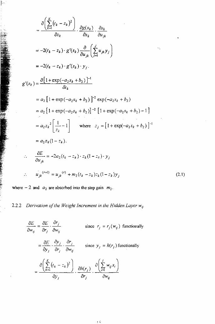
(2.1)

where - 2 and a2 are absorbed into the step gain m2'

2.2.2 Derivation of the Weight Increment in the Hidden Layer wi}

aE at" arj --=_._- since 'j = 'j (wi}) functionally

aE ayj arj =-._._- since y j = h(rj) functionally

I' "

where

a(~(tk-z,)2) , = oh(~)ox. Oyj I I

K

= I (-2)(tk -ZdoZk o(l-zk)ujk oh'(rj)·xi k=l

K

= I (-2)(t k - Z k ) 0 Z k ° (1 - z du jk ° Y j 0 (1 - Y j ) 0 Xi

k=1

(2.2)

Having derived the backpropagation training equation to minimize the partial sum of

squared errors function E(q) for any fixed qth exemplar pair (x(q), ,(q»), an

implementation of the error backpropagation can be done using the flowchart in

Figure 2.2. After all the Q exemplar pairs have been trained in each cycle, an epoch has

been completed.

input/read data (yfq), Iq"» input no. of epochs R, set parameters ai , bi , mi , i = 1, 2

generate initial weights w·(I) u (\)

Ij , lie

.' .' set number of epochs r=l

set number of exemplars, q = 1

compute output i q)

update weights

(r+l) wi}

V+l) II jk

(r) DE( W,u) = IIjk + m, -. -

- dl jk

YES

NO r = r+ 1 1<--------<' Is r> R1

q = q+ 1

NO

Is q> Q? )-________ --1

YES

Figure 2.2 Backpropagation flowchart for the single hidden layer MLP.

I'

2.3 Extension of the Error Backpropagation Algorithm to Two Hidden Layers

Relatively little is known concerning the advantages and disadvantages of using a single

hidden layer with many units (neurons) over many hidden layers with fewer units.

Some authors see little theoretical gain in considering more than one hidden layer since

.. a single hidden layer model suffices for density or a good approximation (Pinkus,

.1999). One important advantage of the multiple (rather than single) hidden layer has to

do with the existence of a locally supported or at least 'localized' function in the two

... hidden layer model.

An extended architecture from Figure 2.1 is shown in Figure 2.3 with two hidden layers.

The interconnection weights for the input/output training pairs

{ (x(q) ,t(q)): q = 1, 2, '" , Q} are Ujk with f. = 1, 2, ... , L,

i = 1 2 .'. J J. = 1 2 ... J and k = 1 2 ... K (where k is normally taken to be 1 ."" '" '"

for the approximation problem). We derive the computational formulae for updating the

weights via steepest descent in the extended backpropagation algorithm using similar

sigmoidal functions as in the case of the single hidden layer.

first hidden second hidden output layer

L I J

true value

Ci = p(ni ) = P("'i.vn,Xt}, Yi = h(rj) ~ hCL.Wij,Ci), ::k = g(sd = g(Lujk>Yj) t~l i=1 j~1

Figure 2.3 The extended two hidden layer neural network.

IS

The partial derivatives in the weight updates are as follows:

(r+1) (r) 8E(vu,wij,Ujk) v li = V li + mO ---~---".-"--,

UVli

We use the same parameter names and indices for the output layers in Figures 2.1

and 2.3. The second hidden layer is the hidden layer adjacent to the output layer. Using

Eq.(2.1) for the increment on U jk' the weights from the second hidden layer to the'

..... output layer, we have

The difference in the variable designations here as compared to the case of a single

hidden layer in Section 2.2 is the input Xl = (XI' "', xL)and the additional first hidden

layer weights cj = (cl , "', c[). The corresponding weights from the input to the first

hidden layer are v li' The updates in the weights from the first to the second hidden

layer, upon making changes to Eq.(2.2) are:

K (r+l) (r) '" ( _ ) _ (1 -) (r) (1 ) wij = wij +mlL. tk --k '-k' --k ujk 'Yj' -Yj -C j •

k=1

Let p be the sigmoidal activation function for the first hidden layer. The value of the

neuron in the first hidden layer

L for ni = L:Vu X £ where ao and bo are the corresponding rate factor and bias

£=1

respectively.

'. The derivation of the weight updates at the first hidden layer is more tedious and we

suppress the q subscripts as compared to the derivation in Section 2.2.

The total sum of squared errors

= f (tk - g(±Ujkhcrj)JJ2 k=1 }=1

= f (tk - g(±Ujkh(± Wy.CiJJJ2 k=! }=I 1=1

= f (tk - g (± U jk h (± wij p(ni )JJJ2 k=1 }=I 1=1

= f(tk -g(± UJkh(± Wijp(± Vli XfJJJJ2 k=1 }:I 1=1 f=1

(2.3)

It can be seen from Figure 2.3 and Eq.C2.3) that each weight Vu at the first hidden layer

affects not only every difference tk - =k but also the value in every unit in the second

2()

hidden layer. To derive aE / Ovii> we need to sum the total error adjustments over all

the units from j = 1, ... , J and k = 1, ... , K. Thus, we use

(2.4)

. From Eq.(2.4), we can write down the chain rule in terms of dependent variables that

start at the output layer and we work backwards to the first hidden layer. This leads to

the partial derivative

aEjk / = (aEjk / ) (azk / ) /Ovt; /azk /Ovlj

= (aEjk / ) (azk / ) (ask/ ) /azk /ask /Ovli

= (aEjk / ) (azk / ) (ask/ ) (ayj / ) /azk /ask /ayj IOva

= (aE~k) (azYaSk) (a%j)(ay~j) (a~li)

= (aE~k) (azYa:k) (a%j) (ay~j) (a%;) (8Yavli)

= (aE ~k) (a=Ya:k) (a%j) (ay ~j) (a%;) (aYanJ (a;lavtJ

(2.5)

The derivatives above all have the same form of 0(1- B). Substituting the derivatives

into Eq.(2.5) and absorbing the 2 into mo just as in Section 2.2, we obtain the

(r + 1) st iterate

~I

We sum up for k = 1, ---, K and j = 1, ---, J to obtain the final update

K J

v[j(r+!) =Vlj(r) +mOL[(tk -Zd-Zk -(l-zk)]L[Ujk 'YJ -(I-Yj)-wij]·c;(l-cj)'Xt· K=! j=!

To summarize the learning equation for updating the weights in the two hidden layers MLP,

we have

2.4 Issues Related to the Implementation of the MLP

The gradient training of MLPs encounters much problematic behaviour unfortunately.

The problems encountered in the use of the backpropagation method as a new tool led

to some failures which were actually due to one or more of these problems. Some

works give bounds on the number of nodes needed to realize a desired approximation.

In general, the bounds depend also on the method used to measure the complexity of the

approximated function and on whether the proof is constructive. Thus, a satisfactory

comparison is difficult (Scarselli & Tsoi, 1998). In addition to an optimum number of

hidden nodes, there is also the problem of testing irrelevant hidd~n units. The work of

Davies (1977) appears relevant in testing the irrelevant hidden unit. The number of

nodes and the convergence rate are related. If we want to approximate a sutliciently

smooth function , using the form :::, with n neurons and using a bounded activation

function (for example, the sigmoidal function), Jones (1992) showed that the

, )

convergence for L2 approximation is 0 (1 / J;;). A heuristic reason why the projection

;~ method in the MLP might work well with a modest number of hidden units is that the

first stage allows a projection onto a subspace of much lower dimensionality within

. which the approximation can be performed .

. The quality of an artificial neural network estimate depends on the number of subjects

or data available with the estimate improving as the number of subjects increases

(Brown, Branford & Moran, 1997). They also showed that the results obtained when

neural networks are applied to survival data depend critically on the treatment of . .

censoring in the data. There may be a large amount of noisy and missing data.

The learning requires careful and generalized training with validation and verification

testing being a crucial stage.

Early stopping using a validation set or early stopping using a fixed training level error

is one of the methods that aim to prevent overtraining due to too powerful a model

class, noisy training examples or a small training set. Cataltepe, Abu-Mostafa &

Magdon-Ismail (1999) analyzed early stopping at a certain training error minimum and

showed that one should minimize the training error as much as possible when all the

information available about the target is the training set. They also demonstrated that

when additional information is available early stopping could help. When the number of

training data becomes infinitely large and they are unbiased, the network parameter

converges to one of the local minima of the empirical risk function (expected loss) to be

minimized. When the number of training data is finite, the true risk function

(generalization error) is different from the empirical risk function. Thus, since the

training examples are biased, the network parameters converge to a biased solution.

This is known as overfitting or overtraining because the parameter values fit too well

the speciality of the biased training example and are not optimal in the sense of

tDinimizing the generalization error given the risk fimction. There are a number of

.. methods to avoid overfitting like, for example, model selection methods by Murata,

Yoshizawa & Amari (1994). For optimum performance when the number of

parameters, m, is large, we should use almost all the t examples in the training set and

only (t / ..J2m)% for cross validation (Amari et aI., 1997). In the asymptotic phase

where t is sufficiently large, the asymptotic theory of statistics is applicaole and the

estimated parameters are approximately normally distributed around the true values.

There are several ways to improve the generalization capability of a neural network.

One is to collect more training data. This may be difficult for some applications and it

is not clear when the amount of training data is enough. The other approach is to

constrain the neural network so that it fits the problem. Jean & Wang (1994)

incorporate a smoothing constraint into the objective function of the backpropagation to

seek a solution with smoother connection weights. They develop a weight-smoothing

algorithm for that purpose and the resulting network generalized better as confirmed by

simulations.

For capacity and universality in application to functional approximation, it is apparently

better for the number of hidden nodes to be as large as possible. Lawrence, Giles & Tsoi

(1997) found that the backpropagation fails to find an optimal solution in many cases.

Furthermore, networks with more weights than might be expected can result in lower

training and generalization errors in certain cases as MLP trained with backpropagation