FULL VEHICLE DYNAMICS MODEL OF A FORMULA SAE...

FULL VEHICLE DYNAMICS MODEL OF A

FORMULA SAE RACECAR USING ADAMS/CAR

A Thesis

by

RUSSELL LEE MUELLER

Submitted to the Office of Graduate Studies of Texas A&M University

in partial fulfillment of the requirements for the degree of

MASTER OF SCIENCE

August 2005

Major Subject: Mechanical Engineering

FULL VEHICLE DYNAMICS MODEL OF A

FORMULA SAE RACECAR USING ADAMS/CAR

A Thesis

by

RUSSELL LEE MUELLER

Submitted to the Office of Graduate Studies of Texas A&M University

in partial fulfillment of the requirements for the degree of

MASTER OF SCIENCE

Approved by: Chair of Committee, Make McDermott Committee Members, Arun R. Srinivasa

Glen N. Williams Head of Department, Dennis L. O’Neal

August 2005

Major Subject: Mechanical Engineering

iii

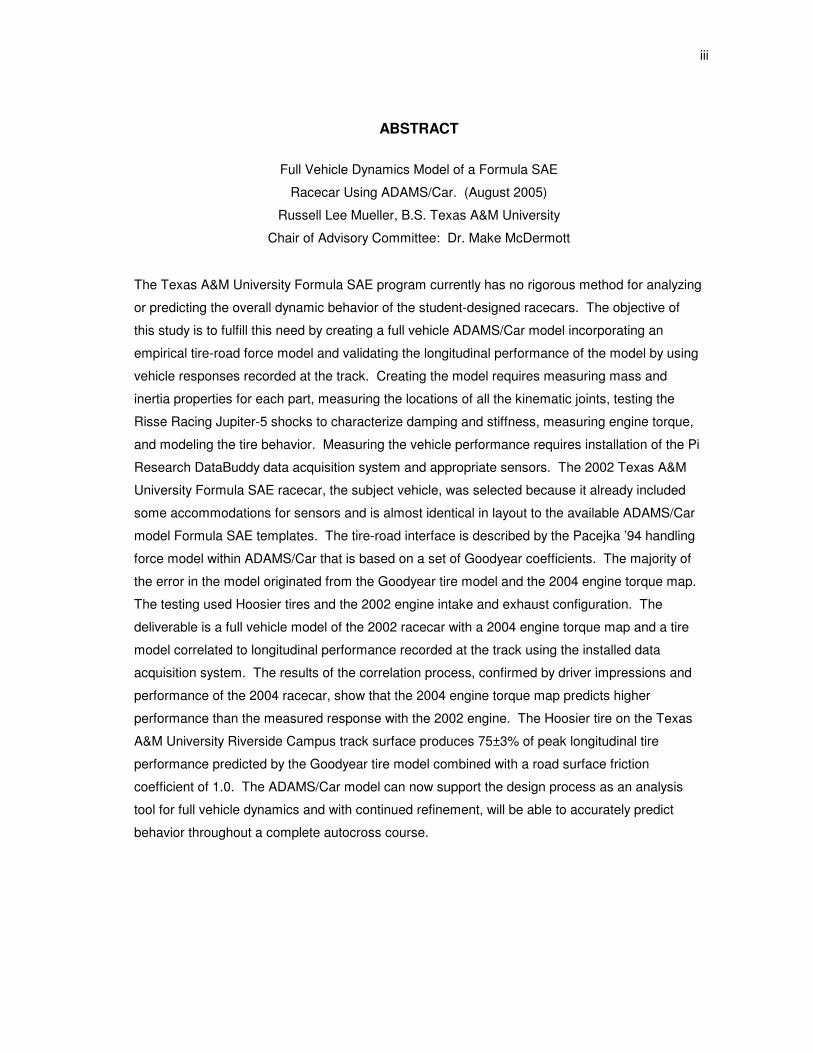
ABSTRACT

Full Vehicle Dynamics Model of a Formula SAE

Racecar Using ADAMS/Car. (August 2005)

Russell Lee Mueller, B.S. Texas A&M University

Chair of Advisory Committee: Dr. Make McDermott

The Texas A&M University Formula SAE program currently has no rigorous method for analyzing

or predicting the overall dynamic behavior of the student-designed racecars. The objective of

this study is to fulfill this need by creating a full vehicle ADAMS/Car model incorporating an

empirical tire-road force model and validating the longitudinal performance of the model by using

vehicle responses recorded at the track. Creating the model requires measuring mass and

inertia properties for each part, measuring the locations of all the kinematic joints, testing the

Risse Racing Jupiter-5 shocks to characterize damping and stiffness, measuring engine torque,

and modeling the tire behavior. Measuring the vehicle performance requires installation of the Pi

Research DataBuddy data acquisition system and appropriate sensors. The 2002 Texas A&M

University Formula SAE racecar, the subject vehicle, was selected because it already included

some accommodations for sensors and is almost identical in layout to the available ADAMS/Car

model Formula SAE templates. The tire-road interface is described by the Pacejka ’94 handling

force model within ADAMS/Car that is based on a set of Goodyear coefficients. The majority of

the error in the model originated from the Goodyear tire model and the 2004 engine torque map.

The testing used Hoosier tires and the 2002 engine intake and exhaust configuration. The

deliverable is a full vehicle model of the 2002 racecar with a 2004 engine torque map and a tire

model correlated to longitudinal performance recorded at the track using the installed data

acquisition system. The results of the correlation process, confirmed by driver impressions and

performance of the 2004 racecar, show that the 2004 engine torque map predicts higher

performance than the measured response with the 2002 engine. The Hoosier tire on the Texas

A&M University Riverside Campus track surface produces 75±3% of peak longitudinal tire

performance predicted by the Goodyear tire model combined with a road surface friction

coefficient of 1.0. The ADAMS/Car model can now support the design process as an analysis

tool for full vehicle dynamics and with continued refinement, will be able to accurately predict

behavior throughout a complete autocross course.

iv

NOMENCLATURE

ACAR ADAMS/Car Software

ARB Anti-Roll Bar

B Pacejka '94 Handling Force Model – Stiffness Factor

BCD Pacejka '94 Handling Force Model – Stiffness

BCDLON or LAT Pacejka '94 Handling Force Model – Stiffness Adjustment

b0-b13 Pacejka '94 Handling Force Model – Longitudinal Tire Coefficients

BUS Bushing

C Pacejka '94 Handling Force Model – Shape Factor

CAD Computer Aided Drafting or Design

CEA Pi Research Club Expert Analysis Software

CG Center of Gravity

CNV Kinematic Joint – Constant Velocity

CYL Kinematic Joint – Cylindrical

D Pacejka '94 Handling Force Model – Peak Factor

DAQ Data Acquisition

DLON or LAT Pacejka '94 Handling Force Model – Peak Factor Adjustment

DOF Degree(s) of Freedom

E Pacejka '94 Handling Force Model – Curvature Factor

ECU Engine Control Unit

FIX Kinematic Joint – Fixed

FSAE Formula SAE

HOK Kinematic Joint – Hooke

INL Kinematic Joint – Inline

INP Kinematic Joint – Inplane

κ Pacejka '94 Handling Force Model – Longitudinal Slip Ratio

MAP Intake Manifold (plenum) Air Pressure Sensor

MKS ADAMS/Car Units – Meters, Kilograms, Seconds

MMKS ADAMS/Car Units – Millimeters, Kilograms, Seconds

ORI Kinematic Joint – Orientation

PAX Kinematic Joint – Parallel_axes

PER Kinematic Joint – Perpendicular

PiDB Pi Research DataBuddy Logger

PLA Kinematic Joint – Planar

REV Kinematic Joint – Revolute

v

SAE Society of Automotive Engineers

SH Pacejka '94 Handling Force Model – Horizontal Shift

SI International System of Units

SLA Short-Long Arm Suspension

SPH Kinematic Joint – Spherical

SV Pacejka '94 Handling Force Model – Vertical Shift

TAMU Texas A&M University

TEES Texas Engineering Experiment Station

TPS Throttle Position Sensor

TRA Kinematic Joint – Translational

V6 Pi Research Version 6 Software

X Pacejka '94 Handling Force Model – Composite Slip Ratio

vi

TABLE OF CONTENTS

Page

ABSTRACT.....................................................................................................................................iii

NOMENCLATURE..........................................................................................................................iv

TABLE OF CONTENTS..................................................................................................................vi

LIST OF FIGURES ....................................................................................................................... viii

LIST OF TABLES .......................................................................................................................... xi

INTRODUCTION ............................................................................................................................ 1

Objective ..................................................................................................................................... 1 Background ................................................................................................................................. 1

PROCEDURE................................................................................................................................. 3

MODEL DESCRIPTION ................................................................................................................. 4

Model Scope ............................................................................................................................... 4 Coordinate Systems.................................................................................................................... 5 Kinematic Joints .......................................................................................................................... 5 Subsystems................................................................................................................................. 7

Chassis Subsystem ................................................................................................................. 7 Front Suspension Subsystem.................................................................................................. 8 Rear Suspension Subsystem .................................................................................................. 9 Anti-Roll Bar Subsystem.......................................................................................................... 9 Steering Subsystem .............................................................................................................. 10 Wheel and Tire Subsystem ................................................................................................... 11 Brake Subsystem .................................................................................................................. 11 Powertrain Subsystem........................................................................................................... 11

Sub-Models ............................................................................................................................... 12 Shocks................................................................................................................................... 13 Differential ............................................................................................................................. 14 Powertrain.............................................................................................................................. 14 Tires....................................................................................................................................... 15 Driver, Road, and Straight-Line Acceleration Event Setup.................................................... 17

SUB-MODEL AND SUBSYSTEM DATA COLLECTION.............................................................. 19

Kinematic Joints ........................................................................................................................ 19 Vehicle CG ................................................................................................................................ 21 Mass and Inertia........................................................................................................................ 23 Engine Torque Map................................................................................................................... 23 Shock Damping and Stiffness Testing ...................................................................................... 25

VEHICLE RESPONSE.................................................................................................................. 28

Data Acquisition System ........................................................................................................... 28 Logger ................................................................................................................................... 28 Wheel Speed......................................................................................................................... 29 Suspension Travel................................................................................................................. 30 Steering Wheel Angle............................................................................................................ 31 Beacon and Lap Layout......................................................................................................... 31 Engine Speed ........................................................................................................................ 31

vii

Page

Throttle Position..................................................................................................................... 32 Sampling Rate ....................................................................................................................... 32 Miscellaneous DAQ System Suggestions ............................................................................. 32

Vehicle Response Testing ........................................................................................................ 33 System Configurations .......................................................................................................... 33 Procedure .............................................................................................................................. 34 Post-Processing .................................................................................................................... 36

MODEL CORRELATION .............................................................................................................. 38

Comparison of Simulated and Measured Responses............................................................... 38 Configuration 1 ...................................................................................................................... 39 Configuration 2 ...................................................................................................................... 39 Configuration 3 ...................................................................................................................... 39 Configuration 4 ...................................................................................................................... 39 Overall Observations ............................................................................................................. 40

Conclusions............................................................................................................................... 41

RECOMMENDED NEXT STEPS ................................................................................................. 42

SUMMARY.................................................................................................................................... 43

REFERENCES ............................................................................................................................. 44

APPENDIX A FIGURES ............................................................................................................. 45

APPENDIX B TABLES................................................................................................................ 94

VITA............................................................................................................................................ 113

viii

LIST OF FIGURES

Page

Figure 1: Coordinate System Orientation..................................................................................... 46

Figure 2: Front Suspension Subsystem....................................................................................... 47

Figure 3: Rear Suspension Subsystem ........................................................................................ 48

Figure 4: Front Suspension Subsystem Parts ............................................................................. 49

Figure 5: Rear Suspension Subsystem Parts.............................................................................. 49

Figure 6: Anti-Roll Bar Subsystem Parts ..................................................................................... 50

Figure 7: Steering Subsystem Parts ............................................................................................ 50

Figure 8: Coil-Over Shock Sub-Model ......................................................................................... 51

Figure 9: Suspension Springs...................................................................................................... 51

Figure 10: Suspension Dampers ................................................................................................. 52

Figure 11: Viscous Differential ..................................................................................................... 52

Figure 12: Normal Load Effects on Normalized Longitudinal Tire Force..................................... 53

Figure 13: Scaling Effects on Normalized Longitudinal Tire Force.............................................. 53

Figure 14: Simulation Setup – Full-Vehicle Analysis Straight-Line Acceleration ......................... 54

Figure 15: Kinematic Joint Locations – First Laser Level Orientation (y direction)...................... 55

Figure 16: Kinematic Joint Locations – Second Laser Level Orientation (x direction) ................ 56

Figure 17: Hardpoint Measurement Using a Laser Level ............................................................ 56

Figure 18: SolidWorks Model for Estimating Inertia .................................................................... 57

Figure 19: Powertrain Subsystem Engine Torque Map ............................................................... 58

Figure 20: Risse Racing Jupiter-5 Shock #1 – Total Force, All 5 Tested Settings ...................... 59

Figure 21: Risse Racing Jupiter-5 Shock #1 – Damping, MID Bump + MID Rebound................ 60

Figure 22: Risse Racing Jupiter-5 Shock #1 – Damping, MID Bump + HI Rebound................... 60

Figure 23: Risse Racing Jupiter-5 Shock #1 – Damping, MID Bump + LOW Rebound.............. 61

Figure 24: Risse Racing Jupiter-5 Shock #1 – Damping, HI Bump + MID Rebound................... 61

Figure 25: Risse Racing Jupiter-5 Shock #1 – Damping, LOW Bump + MID Rebound.............. 62

Figure 26: Risse Racing Jupiter-5 Shock #1 – Stiffness (Speed = 0.13 mm/s)........................... 62







ix

Page









Figure 41: DAQ Installation – Pi DataBuddy Logger.................................................................... 71

Figure 42: DAQ Installation – Front Wheel Speed Sensor .......................................................... 72

Figure 43: DAQ Installation – Rear Wheel Speed Sensor........................................................... 73

Figure 44: DAQ Installation – Front Suspension Travel .............................................................. 74

Figure 45: DAQ Installation – Rear Suspension Travel ............................................................... 75

Figure 46: DAQ Installation – Steering Wheel Angle................................................................... 76

Figure 47: DAQ Installation – Beacon Receiver .......................................................................... 76

Figure 48: Configuration 1 – Filtered Rear Wheel Speed and Longitudinal Slip Ratio ................ 77

Figure 49: Configuration 1 – Longitudinal Chassis Acceleration ................................................. 78

Figure 50: Configuration 1 – Engine Speed................................................................................. 78

Figure 51: Configuration 1 – Longitudinal Chassis Speed........................................................... 79

Figure 52: Configuration 1 – Longitudinal Slip Ratio.................................................................... 79

Figure 53: Configuration 1 – Normalized Tire Force vs. Longitudinal Slip Ratio ......................... 80

Figure 54: Configuration 1 – Throttle Position ............................................................................. 80

Figure 55: Configuration 1 – Damper Travel ............................................................................... 81












x

Page











xi

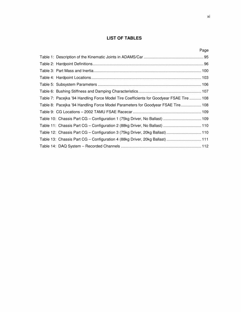
LIST OF TABLES

Page

Table 1: Description of the Kinematic Joints in ADAMS/Car ....................................................... 95

Table 2: Hardpoint Definitions...................................................................................................... 96

Table 3: Part Mass and Inertia................................................................................................... 100

Table 4: Hardpoint Locations..................................................................................................... 103

Table 5: Subsystem Parameters ............................................................................................... 106

Table 6: Bushing Stiffness and Damping Characteristics.......................................................... 107

Table 7: Pacejka ’94 Handling Force Model Tire Coefficients for Goodyear FSAE Tire ........... 108

Table 8: Pacejka ’94 Handling Force Model Parameters for Goodyear FSAE Tire................... 108

Table 9: CG Locations – 2002 TAMU FSAE Racecar ............................................................... 109

Table 10: Chassis Part CG – Configuration 1 (75kg Driver, No Ballast) ................................... 109

Table 11: Chassis Part CG – Configuration 2 (88kg Driver, No Ballast) ................................... 110

Table 12: Chassis Part CG – Configuration 3 (75kg Driver, 20kg Ballast) ................................ 110

Table 13: Chassis Part CG – Configuration 4 (88kg Driver, 20kg Ballast) ................................ 111

Table 14: DAQ System – Recorded Channels .......................................................................... 112

1

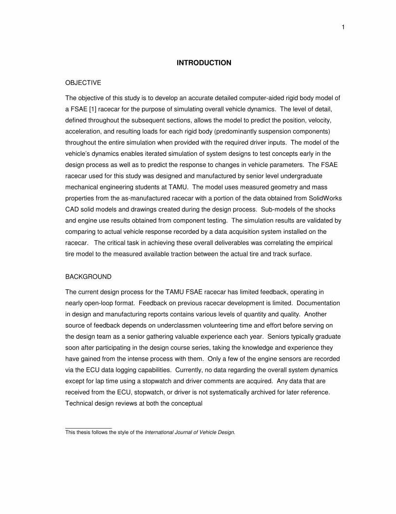
INTRODUCTION

OBJECTIVE

The objective of this study is to develop an accurate detailed computer-aided rigid body model of

a FSAE [1] racecar for the purpose of simulating overall vehicle dynamics. The level of detail,

defined throughout the subsequent sections, allows the model to predict the position, velocity,

acceleration, and resulting loads for each rigid body (predominantly suspension components)

throughout the entire simulation when provided with the required driver inputs. The model of the

vehicle’s dynamics enables iterated simulation of system designs to test concepts early in the

design process as well as to predict the response to changes in vehicle parameters. The FSAE

racecar used for this study was designed and manufactured by senior level undergraduate

mechanical engineering students at TAMU. The model uses measured geometry and mass

properties from the as-manufactured racecar with a portion of the data obtained from SolidWorks

CAD solid models and drawings created during the design process. Sub-models of the shocks

and engine use results obtained from component testing. The simulation results are validated by

comparing to actual vehicle response recorded by a data acquisition system installed on the

racecar. The critical task in achieving these overall deliverables was correlating the empirical

tire model to the measured available traction between the actual tire and track surface.

BACKGROUND

The current design process for the TAMU FSAE racecar has limited feedback, operating in

nearly open-loop format. Feedback on previous racecar development is limited. Documentation

in design and manufacturing reports contains various levels of quantity and quality. Another

source of feedback depends on underclassmen volunteering time and effort before serving on

the design team as a senior gathering valuable experience each year. Seniors typically graduate

soon after participating in the design course series, taking the knowledge and experience they

have gained from the intense process with them. Only a few of the engine sensors are recorded

via the ECU data logging capabilities. Currently, no data regarding the overall system dynamics

except for lap time using a stopwatch and driver comments are acquired. Any data that are

received from the ECU, stopwatch, or driver is not systematically archived for later reference.

Technical design reviews at both the conceptual

This thesis follows the style of the International Journal of Vehicle Design.

2

and detail level from outside reviewers with various levels of experience, knowledge, and

understanding of the design provide feedback based on the students’ presentations of the

design. Presentations are severely limited in detail due to time constraints. The outside

participation is from volunteers who donate their time and expertise while undergraduate

mechanical engineering seniors usually have a full schedule of coursework in addition to FSAE.

Design, manufacturing, and testing all occur at an accelerated pace throughout the entire

process which proceeds from a clean sheet of paper design to fully functional and endurance-

tested vehicle ready for competition in less than nine months.

Possibly because of the lack of feedback or the fast-paced densely-packed schedule, analysis

tools for overall vehicle dynamics are not utilized. Instead, analysis of steady-steady state

behavior, driver impressions, lap times, and past designs determine the envelope for future

suspension design parameters. Steady-state vehicle behavior and suspension geometry is

evaluated using fundamental analysis methods derived by Gillespie [2]. The suspension

subsystem design is iterated to achieve desired values of computed parameters per Milliken [3].

The desired parameter values are based on “rules of thumb”, not performance criteria. Multiple

iterations of overall system design are limited because of time and funding constraints in the

current process. A single iteration evolves through the design, manufacture, and competition of

an entirely new racecar with nearly all-new team members, producing one significant test datum

with limited information or documentation per year. The results of this study attempt to reduce

the time between iterations and increase the rate of development both during the initial design

stages and the actual testing prior to competition. The installed data acquisition system will not

only validate the results of the model but also provide output data for closing the development

feedback loop.

3

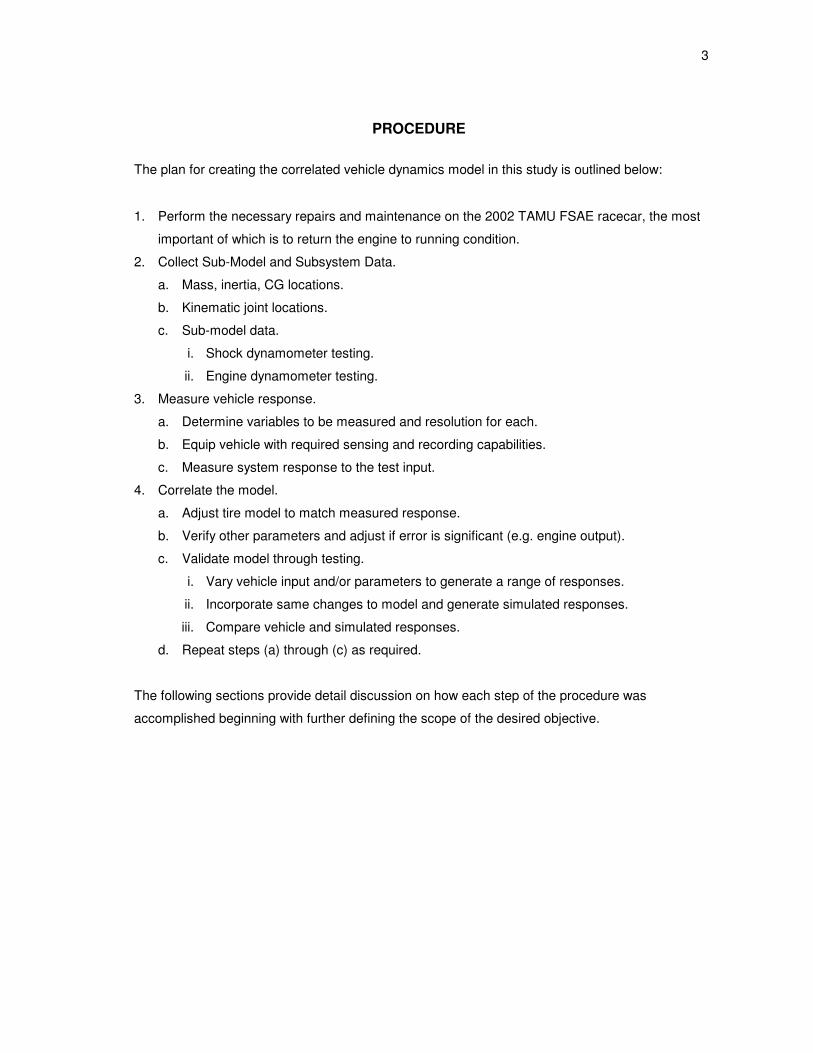
PROCEDURE

The plan for creating the correlated vehicle dynamics model in this study is outlined below:

1. Perform the necessary repairs and maintenance on the 2002 TAMU FSAE racecar, the most

important of which is to return the engine to running condition.

2. Collect Sub-Model and Subsystem Data.

a. Mass, inertia, CG locations.

b. Kinematic joint locations.

c. Sub-model data.

i. Shock dynamometer testing.

ii. Engine dynamometer testing.

3. Measure vehicle response.

a. Determine variables to be measured and resolution for each.

b. Equip vehicle with required sensing and recording capabilities.

c. Measure system response to the test input.

4. Correlate the model.

a. Adjust tire model to match measured response.

b. Verify other parameters and adjust if error is significant (e.g. engine output).

c. Validate model through testing.

i. Vary vehicle input and/or parameters to generate a range of responses.

ii. Incorporate same changes to model and generate simulated responses.

iii. Compare vehicle and simulated responses.

d. Repeat steps (a) through (c) as required.

The following sections provide detail discussion on how each step of the procedure was

accomplished beginning with further defining the scope of the desired objective.

4

MODEL DESCRIPTION

MODEL SCOPE

MSC Software’s ADAMS/Car program and the FSAE templates1 are utilized in this study to

create the complete vehicle dynamics model of the 2002 TAMU FSAE racecar. The reasons for

selecting ACAR are:

1. Capability is more than adequate for the TAMU FSAE program’s needs.

2. Available to TAMU at a reasonable cost.

3. Writer’s past experience in the automotive industry using ACAR.

The FSAE templates are the first and probably most important boundary applied to the scope of

the study because they define the level of complexity for the model and sub-models. Building a

custom template from scratch or drastically modifying the available templates is outside the

scope of this project and the TAMU FSAE program at this time.

The 2002 racecar was selected for graduate research because it was still a completely

assembled vehicle, was not used for driver practice because the engine had not run since the

2002 FSAE competition, and was designed to accommodate data acquisition. The major

obstacle was getting the engine to run properly. However, the 2002 racecar design did not

require major modifications to the ACAR templates. This benefit more than compensates for

having to repair the engine since it reduces the opportunity for the model to generate problems or

errors, resulting in more time spent on model correlation and less time spent on debugging the

model.

The ACAR model is capable of much more than the present data acquisition system can

measure for validation, which brings up the next major limit on the scope of this study – tire data.

In a road vehicle, the overall response of the vehicle is highly sensitive to the tire-road interface.

Obtaining an accurate model for the tire-road interface is a common problem for full vehicle

dynamics model as tire forces depend on several variables: temperatures of the tire surface and

carcass, pressure, wear, age, prior use, manufacturing variability, and of course the

1ADAMS/Car Formula SAE Templates originally developed by the University of Michigan Formula SAE Racing Team

and are available from MSC Software at

http://university.adams.com/student_competitions/templates/templates_main.htm [accessed June 2005].

5

condition of the road surface to name a few. The tire model, discussed later in detail, receives

tire contact patch conditions such as slip magnitude, slip direction, applied normal force, and

wheel camber as input and returns the corresponding tire handling forces, or “grip” level.

Accurately measuring the slip or the resulting forces at the tire-road interface is difficult,

expensive, and usually approximated. With the available funding, sensor capabilities limit

measured tire data to the longitudinal slip direction, x. The section on data acquisition covers

how the longitudinal slip is measured and the associated approximation. The normal force

applied to the tire is not measured directly but instead is calculated using the measured

acceleration and the measured vehicle mass and geometry.

Working within these constraints, the study results in a complete ACAR vehicle dynamics model

correlated in the longitudinal direction, ready for further improvements from increased capabilities

in data acquisition or research funding in the future. The following sections describe the ACAR

model as defined by the FSAE templates, which determines the necessary measurements

required in the procedure.

COORDINATE SYSTEMS

Two coordinate systems will be used. The fixed ground Cartesian coordinate system is defined

by unit vectors X, Y, and Z. The vehicle Cartesian coordinate system has unit vectors x, y, and z

and is initially at time t = 0s coincident with the ground coordinate system (Figure 1). The x unit

vector is aligned along the vehicle longitudinal centerline with the positive direction pointing

towards the rear. The z unit vector is nominally vertical with the positive direction pointing

towards the top of the vehicle. Using a right-hand system, the y unit vector positive direction

must point towards the driver’s right side. Typically, the location of the origin of vehicle

coordinate system is chosen for convenience in measuring vehicle geometry. The x-y plane is

placed slightly below the tires and the y-z plane some distance in front of the racecar, but these

are not critical. ACAR determines the ride height during initial setup of the simulation. The x-z

plane is the plane of symmetry for vehicles with identical left and right geometry but this is not

always true. ACAR and the FSAE templates can accommodate an asymmetric vehicle if

necessary.

KINEMATIC JOINTS

Kinematic joints are named to describe the mathematical constraint equations they create on the

kinematics of the attached rigid bodies [4, p128]. An example found frequently throughout this

6

model is a spherical joint, a.k.a. “ball-and-socket” joint, which constrains the three translational

DOF while allowing the three rotational DOF. Table 1 describes each type of kinematic joint as

defined by ACAR2. The spherical bearings or “rod ends” used at suspension joints on FSAE

racecars behave as SPH joints over the design range of motion. Note the Hooke joint is identical

to a SPH joint except the rotational DOF corresponding to the spin axis is constrained. The

typical application for a HOK joint in the ACAR FSAE template is on a rod with a SPH joint at the

other end. In effect, the HOK joint removes a free rotational DOF along the rod’s spin axis if it

instead had SPH joints at both ends.

The bushing is another type of connection modeled in ACAR which allows all six DOF to occur

with resulting forces and moments defined by stiffness and damping parameters. The bushing is

not listed as a kinematic joint since it does not apply DOF constraint equations on the attached

rigid bodies. The ACAR FSAE template does incorporate bushings at various joints for added

freedom when adapting the template to suit the specific subject vehicle. For the 2002 TAMU

FSAE racecar and many other racecars, the spherical bearings, as well as the other types of

bearings used throughout the entire car, have very high stiffness, low friction, and little or no free-

play present. Bushings are more suited to the lower stiffness and higher damping characteristics

of production automotive applications in elastomeric engine or suspension mounts. Where

bushings have been included in the FSAE template, the stiffness and damping parameters have

been adjusted to match the behavior of the FSAE racecar bushing applications.

ACAR can couple DOF in cases where the desired motion is not represented by the predefined

kinematic joints or a bushing. For example, a rack and pinion is modeled by coupling the

rotational DOF of the pinion to the translational DOF of the rack at some gear reduction. The

coupled DOF by ACAR will then generate a constraint equation on the relative motion between

the two parts at the specified reduction.

2ADAMS/Car Help Documentation > Components > Attachments > Joints.

7

SUBSYSTEMS

ACAR uses a set of templates to create the full vehicle model as an assembly of subsystems.

The following sections describe each subsystem in relation to the 2002 TAMU FSAE racecar.

Refer to the ACAR help documentation for further detail regarding specifics of how the software

utilizes the templates. The discussion here is intended to cover the rigid body dynamics of the

full vehicle model. Refer to Tables 2-6 which list the hardpoint definitions, part mass and inertia

properties, hardpoint locations, any relevant parameters, and bushing characteristics respectively

for each subsystem (unless otherwise noted).

Chassis Subsystem

The chassis subsystem contains a single rigid body, or part, that defines the location of all the

vehicle components that are non-rotating and fixed relative to the vehicle coordinate system, e.g.

frame, bodywork, driver, radiator, wiring, ballast, etc. The engine and transmission, included

within the powertrain subsystem described later, is the one exception to this rule. For visual

purposes, a solid model of the 2002 FSAE frame was attached in ACAR to the chassis part

(Figure 1). Mass and inertia properties of the chassis part depends on the configuration of the

vehicle being tested and is varied to achieve the desired overall vehicle CG location and total

mass. The following subsystems build off the chassis part to create the full vehicle assembly:

• front and rear suspension

• steering

• powertrain

• front and rear wheels/tires

• brakes

• front and rear anti-roll bars

Parameters are associated with the chassis subsystem for approximating the aerodynamic drag

opposing forward velocity of the vehicle: frontal area, air density, and coefficient of drag. ACAR

assumes these parameters are in SI units despite the system of units chosen for the full vehicle

model. SI units are referred to by ACAR as the MKS system of units for meters, kilograms, and

seconds. Based on experiences in this study, it is highly recommended to use either MKS or

MMKS (for mm, kg, and s) to remain consistent. The user should choose either MKS or MMKS

to minimize variation of the matrix entries in the system of equations. ACAR is more efficient at

solving the equations if the non-zero matrix values are all of similar orders of magnitude.

8

Front Suspension Subsystem

The function of the front suspension subsystem is to control the independent motion of each front

wheel relative to the chassis. The wheels are allowed to precess (controlled by the steering

subsystem) and spin independently (controlled by the braking system). The overall layout and

individual part descriptions are shown in Figures 2 and 4 with the wheel/tire subsystem excluded

for clarity. The axis of the wheel is nominally aligned with the hub axis. The front suspension

subsystem design for this vehicle is symmetric about the x-z plane. Part mass and inertia

properties or joint locations can be defined asymmetrical in the model to reflect the actual vehicle

if necessary.

The front suspension design used on the 2002 TAMU FSAE racecar is described as a fully

independent SLA with push rod actuated coil-over shock. Each side of the suspension forms a

three-dimensional version of a four-bar linkage in order to control the four DOF (three

translations, one rotation) of each front upright with a desired amount of stiffness and damping.

The hub allows the spin DOF of the wheel with respect to the upright. The upright and hub then

precess as the upright rotates about an axis through the upper and lower control arm joints (ball

joints) to accommodate the steering subsystem.

The coil-over shock is a damper and coil spring combination. The shock itself is a multi-

component dynamic device that will be approximated by a sub-model described later in further

detail. The shock is actuated by a bellcrank, or rocker, that transfers the relative motion of wheel

and chassis from the push rod attached to the lower control arm. The final linkage is a steering

link attaching the steering subsystem to the suspension.

Hardpoints in ACAR are the parametric locations that define where to place the joints and offer

the ability to adjust suspension geometry very quickly and easily. The number of joints and the

number of hardpoints are not usually equal because some joints share hardpoint locations or are

pre-defined relative to other suspension geometry. The template maintains the overall

subsystem layout but adjusts the parts’ dimensions to fit the hardpoints. The front suspension

template uses parameters to adjust the left and right camber and toe angles without having to

relocate the hardpoints.

9

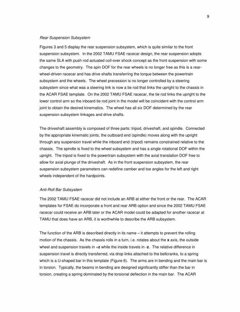
Rear Suspension Subsystem

Figures 3 and 5 display the rear suspension subsystem, which is quite similar to the front

suspension subsystem. In the 2002 TAMU FSAE racecar design, the rear suspension adopts

the same SLA with push rod actuated coil-over shock concept as the front suspension with some

changes to the geometry. The spin DOF for the rear wheels is no longer free as this is a rear-

wheel-driven racecar and has drive shafts transferring the torque between the powertrain

subsystem and the wheels. The wheel precession is no longer controlled by a steering

subsystem since what was a steering link is now a tie rod that links the upright to the chassis in

the ACAR FSAE template. On the 2002 TAMU FSAE racecar, the tie rod links the upright to the

lower control arm so the inboard tie rod joint in the model will be coincident with the control arm

joint to obtain the desired kinematics. The wheel has all six DOF determined by the rear

suspension subsystem linkages and drive shafts.

The driveshaft assembly is composed of three parts: tripod, driveshaft, and spindle. Connected

by the appropriate kinematic joints, the outboard end (spindle) moves along with the upright

through any suspension travel while the inboard end (tripod) remains constrained relative to the

chassis. The spindle is fixed to the wheel subsystem and has a single rotational DOF within the

upright. The tripod is fixed to the powertrain subsystem with the axial translation DOF free to

allow for axial plunge of the driveshaft. As in the front suspension subsystem, the rear

suspension subsystem parameters can redefine camber and toe angles for the left and right

wheels independent of the hardpoints.

Anti-Roll Bar Subsystem

The 2002 TAMU FSAE racecar did not include an ARB at either the front or the rear. The ACAR

templates for FSAE do incorporate a front and rear ARB option and since the 2002 TAMU FSAE

racecar could receive an ARB later or the ACAR model could be adapted for another racecar at

TAMU that does have an ARB, it is worthwhile to describe the ARB subsystem.

The function of the ARB is described directly in its name – it attempts to prevent the rolling

motion of the chassis. As the chassis rolls in a turn, i.e. rotates about the x axis, the outside

wheel and suspension travels in +z while the inside travels in -z. The relative difference in

suspension travel is directly transferred, via drop links attached to the bellcranks, to a spring

which is a U-shaped bar in this template (Figure 6). The arms are in bending and the main bar is

in torsion. Typically, the beams in bending are designed significantly stiffer than the bar in

torsion, creating a spring dominated by the torsional deflection in the main bar. The ACAR

10

template for the FSAE racecar assumes rigid body parts to describe the kinematics of the ARB

with a torsion spring/damper element (with zero damping, not shown in figure) included between

the left and right sides. This is usually not an accurate approximation for production automotive

applications but is appropriate for the FSAE racecar.

ACAR uses left and right parts to describe a continuous U-shaped ARB on the vehicle. The ARB

subsystem in the ACAR model consists of 4 parts. The left and right side components are

connected via the torsion spring/damper element in the middle. The REV joint is located at the

midpoint between the left and right arb_bend hardpoints. Note half of the total mass/inertia of the

assembly is applied to each ARB part. A single parameter is provided in the template that

defines the torsional spring rate of the ARB.

Steering Subsystem

Recalling the description of the front suspension subsystem, a rotational DOF is left free for the

wheel to precess and steer the vehicle in the desired heading. The function of the steering

subsystem is to link the driver’s control input to the orientation of the front wheels via the front

suspension subsystem. Input from the driver turns the steering wheel in the desired heading.

The location of the steering wheel usually does not lend itself to using a straight shaft to the rest

of the subsystem because of driver ergonomics. The FSAE template (Figure 7) has three shafts

connected by two HOK joints to accommodate most configurations. The shafts connect the

steering wheel to the rack and pinion assembly transferring the rotation of the shafts and pinion

to linear translation of the geared rack. The tie rods, or steering links, discussed earlier in the

front suspension subsystem are attached to the ends of the rack. As the rack travels, the

steering links push (or pull) on the corresponding upright to steer the front wheels.

ACAR defines the support and rack housing relative to the geometry given for the column and

rack respectively while the pinion joints occupy a singe hardpoint in the model. The outer ends of

the rack are defined by the inboard locations of the steering links in the front suspension

subsystem. The steering subsystem has a single parameter that defines the gear reduction

between the pinion rotation and the rack translation.

11

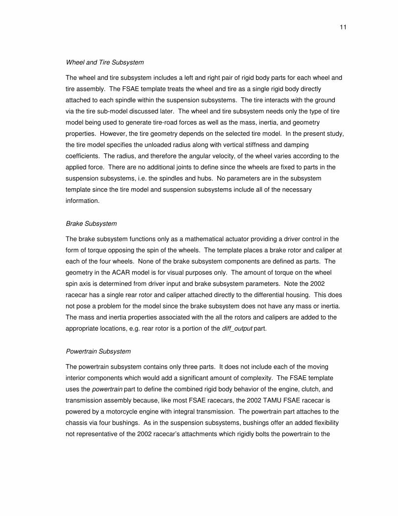
Wheel and Tire Subsystem

The wheel and tire subsystem includes a left and right pair of rigid body parts for each wheel and

tire assembly. The FSAE template treats the wheel and tire as a single rigid body directly

attached to each spindle within the suspension subsystems. The tire interacts with the ground

via the tire sub-model discussed later. The wheel and tire subsystem needs only the type of tire

model being used to generate tire-road forces as well as the mass, inertia, and geometry

properties. However, the tire geometry depends on the selected tire model. In the present study,

the tire model specifies the unloaded radius along with vertical stiffness and damping

coefficients. The radius, and therefore the angular velocity, of the wheel varies according to the

applied force. There are no additional joints to define since the wheels are fixed to parts in the

suspension subsystems, i.e. the spindles and hubs. No parameters are in the subsystem

template since the tire model and suspension subsystems include all of the necessary

information.

Brake Subsystem

The brake subsystem functions only as a mathematical actuator providing a driver control in the

form of torque opposing the spin of the wheels. The template places a brake rotor and caliper at

each of the four wheels. None of the brake subsystem components are defined as parts. The

geometry in the ACAR model is for visual purposes only. The amount of torque on the wheel

spin axis is determined from driver input and brake subsystem parameters. Note the 2002

racecar has a single rear rotor and caliper attached directly to the differential housing. This does

not pose a problem for the model since the brake subsystem does not have any mass or inertia.

The mass and inertia properties associated with the all the rotors and calipers are added to the

appropriate locations, e.g. rear rotor is a portion of the diff_output part.

Powertrain Subsystem

The powertrain subsystem contains only three parts. It does not include each of the moving

interior components which would add a significant amount of complexity. The FSAE template

uses the powertrain part to define the combined rigid body behavior of the engine, clutch, and

transmission assembly because, like most FSAE racecars, the 2002 TAMU FSAE racecar is

powered by a motorcycle engine with integral transmission. The powertrain part attaches to the

chassis via four bushings. As in the suspension subsystems, bushings offer an added flexibility

not representative of the 2002 racecar’s attachments which rigidly bolts the powertrain to the

12

chassis. In the model, the stiffness and damping characteristics of the powertrain bushings

adopt the same characteristics as the suspension control arm bushings.

The powertrain subsystem references two sub-models (sub-models will be discussed in a

subsequent section):

1. Powertrain – defines engine output torque given crankshaft speed and throttle position.

2. Differential – defines an applied torque opposing the given relative shaft speed between left

and right drive shafts.

Do not confuse the powertrain sub-model with the powertrain subsystem. The subsystem

describes the rigid body properties while the sub-model defines torque output only. The

differential sub-model transmits torque from the powertrain sub-model to the left and right

differential outputs while accommodating the independent left and right shaft speeds. The two

parts called diff_output transmit torque from the differential sub-model to each of the drive shafts

defined in the rear suspension subsystem. The mass and inertia properties of the differential are

divided equally across the left and right parts. Parameters within the powertrain subsystem

describe the transmission gear ratios, clutch behavior, engine rotating inertia, etc. As mentioned

earlier, no internal engine components are included but the engine rotating inertia parameter

applies to engine crankshaft speed, approximating the combined overall inertia of the engine’s

rotating and reciprocating components. No inertia is applied to the clutch or transmission.

SUB-MODELS

The FSAE racecar contains several devices with a high level of component complexity such as

the engine, transmission, tires, etc. The available FSAE templates utilize sub-models in order to

simplify the full vehicle model, reduce computational requirements, and still provide an accurate

representation of the overall vehicle dynamics. The shock and engine sub-models are validated

by measuring the response from the individual components.

13

Shocks

The shock used on the 2002 TAMU FSAE racecar has a coil spring installed concentric to the

damper main chamber (Figure 8). For the purpose of this study, it is sufficient to simplify the

shock as the combination of spring stiffness and damping coefficients that determine the force

generated for a given relative suspension position and velocity (Figures 9-10).

The coil spring stiffness, determined by the coil diameter, coil wire diameter, number of coils, and

material properties, has linear behavior until the coils reach the solid stack-up height. ACAR can

use tabular data to describe a variable stiffness as a function of displacement. ACAR uses linear

interpolation between any of the data points to estimate the stiffness. The spring stiffness of the

shock assembly is nonlinear at the travel limits where the shock has elastomer bump-stops with

significantly higher stiffness than the coils. The spring data file, which has the table of spring

force versus displacement as well as the installed spring length (or preload), is referenced within

the suspension subsystem files. The springs used on the 2002 TAMU FSAE racecar are

manufactured at specific stiffness ratings and the manufacturer’s rated stiffness is used as the

baseline stiffness. The shock stiffness, described next, is added in parallel to the coil spring. At

the end of the shock travel, the stiffness transitions to a much higher value to model the bump-

stop installed on the shock shaft for limiting bump travel. Note the limit on travel is different

between the front and rear suspensions. Negative displacements, or stretching of the spring, are

not included since the shock cannot pull on the coil spring.

The shock without the coil spring is predominantly a damper. Without going into great detail on

the design, the damper piston contains orifices that allow fluid to flow from one side of the piston

to the other. The relations among piston speed, flow, orifice resistance to flow, pressure, and

force determine the damper properties. The fluid properties can also vary drastically depending

on such characteristics as temperature or gas build-up in the fluid chamber. The damper has an

additional chamber filled with gas that is separated from the fluid chamber by a floating piston.

The gas allows the piston shaft to displace fluid volume by expanding or contracting according to

the piston travel. As a result, the gas imposes an additional stiffness component to the force

generated by the shock and also depends on temperature. The damping coefficient can be

adjusted by threading tiny needles into or out of fixed orifices to modify the fluid passages within

the shock assembly. Depending on the particular shock design, these adjustments have the

ability to control the damper coefficient at different piston velocities.

14

Similar to the spring data file, ACAR can read in a table of data relating a given input velocity to

the corresponding output force. The damper curve is approximately the middle setting for both

adjustment knobs of the shock and is averaged across the available shock test data. Note the

gas in the shocks generates a static force causing the shock to extend to its limits at rest. This

force is equivalent to a preload on the spring and is defined within the spring data file since an

ACAR damper does not include a static force.

Differential

The differential transmits the torque from the powertrain sub-model to the left and right drive

shafts in the rear suspension subsystem. The differential allows the transfer of torque to both

shafts despite asymmetrical shaft speeds as the vehicle performs various maneuvers. An

additional feature in the 2002 racecar’s differential is the ability to oppose the difference in shaft

speed. For example, if the left wheel begins to spin freely as if on a patch of ice, the input motion

is transmitted to the free spinning left shaft while the right shaft, and therefore the right wheel sits

still. A limited slip differential includes components for opposing the relative shaft speed with an

applied torque to the slower drive shaft. The FSAE powertrain template has the ability to

reference a viscous differential data file which defines the opposing torque versus a given

difference in shaft speed (Figure 11). The 2002 TAMU FSAE racecar utilizes a torque sensing

differential which will not match the ACAR FSAE template but behaves as required for

longitudinal vehicle modeling, e.g. when the difference in shaft speed is negligible.

Powertrain

The powertrain sub-model consists of the engine, clutch, and transmission. The engine

produces torque at a range of crankshaft speeds between idle (minimum) and rev limit

(maximum), at a range of throttle position (driver input), and subject to the engine rotating inertia

parameter. The clutch transmits torque from the engine crankshaft to the transmission given the

clutch position (driver input) and subject to stiffness, damping, and torque threshold parameters.

The transmission transmits torque from the clutch to the differential via a set of selectable gear

ratios (driver input) matching the engine speed to the desired torque and wheel speed.

Beginning with the engine, the FSAE template references a data file similar to the spring or

damper files in the coil-over shock sub-model. The major difference here is that the engine

requires two inputs in order to define the output torque: engine speed and throttle position.

Throttle position, controlled by the driver, determines the amount of air entering the engine for

combustion and therefore directly relates to the amount of torque generated at a given engine

15

speed. The table of engine data must be collected from the TAMU FSAE engine dynamometer,

which measures the torque produced at a given speed and throttle position.

The clutch allows the driver to disconnect the transfer of torque between engine and transmission

during such events as selecting a transmission gear ratio or starting the engine. In this

application, the clutch is a mechanical device that uses friction between rotating discs, similar to

the braking system, to transfer torque between the engine crankshaft and the transmission.

When the driver presses the clutch pedal or lever, the pressure on the disc is removed,

effectively disconnecting the engine from the transmission by no longer transferring torque. To

reapply the clutch pressure, the driver releases the clutch pedal or lever, increasing friction and

the amount of torque transfer. As the friction is determined by the amount of pressure applied

between the clutch discs and the properties of the materials utilized, the amount of torque that

can be transferred is limited and the limit is above the peak torque from the engine. The FSAE

template models the clutch as a torsion spring/damper in parallel between the engine and

transmission. The clutch in this model is approximated as a relatively rigid connection between

engine crankshaft and transmission input shaft.

Tires

The tire model incorporated within the wheel and tire subsystem template predicts behavior given

certain tire contact patch parameters – slip vector, normal force, and orientation (camber angle).

The model developed by Pacejka [5] is referred to by ACAR as the Pacejka ’94 handling force

model. The longitudinal tire force FX along with the lateral tire force FY and self-aligning moment

MZ are the three outputs from the handling force model. The following equations define FX as it

is used by ACAR3:

3ADAMS/Tire Help Documentation > Tire Models > ‘Using ADAMS/Tire Tire Models’ > ‘Using Pacejka ’94 Handling

Force Model’ p83.

16

( )[ ]

( ) ( )[ ]

( )( ) ( )( )

( )( )( )[ ] V11

X

138Z7Z6

H

12Z11V

10Z9H

0Sκ

Z

LONZ5Z4Z3

LONZ2Z1

0

X

SX

SXBtanXBEXBtanCsinDF

Xsignb1bFbFbE

SκX

bFbS

bFbS

DC

BCDB

dκ

dFBCD

BCDFbexpFbFbBCD

DFbFbD

bC

V

Vκ

H

+⋅−⋅⋅−⋅⋅⋅=

⋅−⋅+⋅+⋅=

+=

+⋅=

+⋅=

⋅=

=

⋅⋅−⋅⋅+⋅=

⋅⋅+⋅=

=

−=

−−

=+

The experimentally determined coefficients b0-b13 for the longitudinal tire force model allow the

computation of traction force FX for given values of normal force FZ and longitudinal slip ratio

κκκκ. These coefficients are obtained from extensive tire testing requiring specialized equipment

and several tires in order to apply a complete range of slip and normal force conditions while

recording the resulting tire forces. Producing the empirical tire data for the Hoosier racing tires

used on the TAMU FSAE racecars is outside the scope of the present study. Complete sets of

Pacejka tire coefficients made available to TAMU FSAE correspond to the Goodyear FSAE

racing tires used on a 13” diameter wheel rim with 20” unloaded outside diameter (Tables 7-8)4.

The coefficients are available for either 12psi or 15psi tire pressure and either 6.5” or 8” width but

only those for 6.5” width at 12psi pressure are used here. The TAMU FSAE racecars

predominantly use 7.0” wide Hoosier racing tires due to its past performance in track testing. As

a result, Hoosier is the brand used for the study. The Hoosier tire is 7.0” wide on a 13” diameter

wheel at the 12psi pressure but using a slightly harder compound to extend tire life so that all the

testing can be performed on a single set of tires, reducing cost and tire variability.

4Goodyear tire model Pacejka ’94 coefficients provided by Michael J. Stackpole (Sep 2001), Goodyear Tire and Rubber

Company, Race Tire Development.

17

Despite the many potential differences that could exist between Goodyear and Hoosier, the

performance and behavior of the two brands of racing tire are similar based on past track testing

by TAMU FSAE. However, the Goodyear tire model predicts significantly higher performance

than what has been recorded at the TAMU track using either brand of tire. The available

Goodyear Pacejka coefficients serve only as a starting point for the correlation process with the

expectation that the tire model constitutes the majority of error between the simulation results

and the recorded response at the track. Using the longitudinal tire force equations shown

previously, the normalized longitudinal tire force predicted by the Goodyear model at positive slip

ratios is plotted for three values of normal load in Figure 12. The tire model is adjusted to

correlate with the measured tire performance at the track through the linear scaling factors, DLON

and BCDLON, which adjust the peak factor, D, or the stiffness, BCD, respectively. The effects of

changing these factors are displayed in Figure 13. The scaling for both peak and stiffness are

kept equal in each case, i.e. DLON = BCDLON.

Driver, Road, and Straight-Line Acceleration Event Setup

Much of the driver’s input to the vehicle has already been mentioned in the steering, brake, and

powertrain subsystems. The driver mass and inertias are lumped together with the chassis part.

The driver inputs to the vehicle are: throttle, clutch, brake, transmission gear, and steering wheel.

ACAR has several full vehicle and half vehicle simulations and the capability to develop custom

simulations or driver controls based on data measured at the track. The present study used only

the straight-line acceleration event, which simulates the full vehicle model executing a maneuver

similar to a drag race. ACAR controls the throttle position, transmission gear, and steering inputs

to simulate straight-line acceleration response with several options to customize the event. The

straight-line acceleration event was simulated with the inputs shown in Figure 14. Output prefix

is a character string added to the beginning of each ACAR file produced by the simulation with

“_accel” as the rest of the filename. End time refers to the total time for the event and is

sufficient to allow the full vehicle model to reach the engine 13,500rpm redline. Number of steps

determines the rate at which the ACAR solution marches to the given end time. The time

between each simulation step is kept to 0.01s, i.e. 200 steps for 2.0s, which maintained a good

balance of simulation accuracy and solver efficiency for this study. Initial velocity is the vehicle’s

initial speed at t = 0s and ACAR maintains this speed up until t = start time. At t = start time,

ACAR steps the driver’s throttle control to final throttle at the specified transition time called

duration of step. Gear position is the initial transmission gear for the simulation and the shift

gears toggle is turned off to prevent ACAR from changing gears throughout the event. Steering

18

input is set to “straight line” which tells ACAR to control steering wheel input as required to

maintain the vehicle’s straight line heading.

ACAR uses several road profiles based on the selected simulation or a custom road profile can

be used. The present study only requires a flat ground plane and is defined in the ACAR road

data file. The only parameter is the coefficient of friction, µ. The road data file also includes limit

geometry to describe the size of the ground plane. The coefficient of friction parameter is

equivalent to the adjustment factor, DLON, included in the ACAR Pacejka ’94 handling force model

except that µ applies to both longitudinal and lateral forces. For example, the product DLON x µ is

the total adjustment applied to the longitudinal peak factor, D. Since the study does not

differentiate between tire and road performance, the coefficient of friction for the road surface

remains at 1.0.

19

SUB-MODEL AND SUBSYSTEM DATA COLLECTION

KINEMATIC JOINTS

The actual car differs from the documented design due to manufacturing tolerances or last-

minute design changes that occurred after the drawings were created. In order to improve the

accuracy of the model, the actual vehicle was measured rather than using the existing solid

model drawings. All of the kinematic joints are located by hardpoints defined in the vehicle

coordinate system. Accurately measuring all of the hardpoints on the vehicle is not trivial. The

present study used physical measuring devices because scanning with some form of tomography

was not available. The first obstacle was creating a reference from which to measure all three

Cartesian coordinates. One method considered was a surface plate that would provide an

extremely flat and solid device to mount the vehicle while taking measurements in one

dimension. A surface plate is a thick cast iron plate with a flat milled top surface, several drilled

holes or grooves for mounting measuring devices in various positions, and significant support

underneath to create an extremely rigid measuring surface. The advantage is having a large

solid surface, assuming a large enough surface plate is available, to mount additional measuring

devices or precision blocks to gain access to each joint. The major disadvantage, aside from

finding a surface plate large enough for a racecar, is mounting the vehicle in the three

orientations in order to use the single reference plane.

The option selected for measuring the hardpoints is a laser level that creates two orthogonal

planes, vertical and horizontal, by oscillating a laser beam over a 90deg span. The laser level

used is the self-leveling David White Mark 2 LC Mini Laser Cross Level #48-M2LC. The laser

level is mounted near the vehicle and measurements can be taken from the joint to the plane

created by the laser. Two advantages of using the laser level are that the range of the laser far

exceeds the size of any surface plate and two orthographic planes means only having to change

position once to measure the third dimension. The major disadvantage is finding the normal to a

plane created by a laser since it creates an optical, not physical, measuring plane.

Prior to taking any measurements, the suspension must be locked in place so the geometry does

not change throughout the entire process.

20

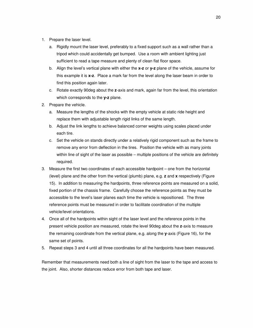
1. Prepare the laser level.

a. Rigidly mount the laser level, preferably to a fixed support such as a wall rather than a

tripod which could accidentally get bumped. Use a room with ambient lighting just

sufficient to read a tape measure and plenty of clean flat floor space.

b. Align the level’s vertical plane with either the x-z or y-z plane of the vehicle, assume for

this example it is x-z. Place a mark far from the level along the laser beam in order to

find this position again later.

c. Rotate exactly 90deg about the z-axis and mark, again far from the level, this orientation

which corresponds to the y-z plane.

2. Prepare the vehicle.

a. Measure the lengths of the shocks with the empty vehicle at static ride height and

replace them with adjustable length rigid links of the same length.

b. Adjust the link lengths to achieve balanced corner weights using scales placed under

each tire.

c. Set the vehicle on stands directly under a relatively rigid component such as the frame to

remove any error from deflection in the tires. Position the vehicle with as many joints

within line of sight of the laser as possible – multiple positions of the vehicle are definitely

required.

3. Measure the first two coordinates of each accessible hardpoint – one from the horizontal

(level) plane and the other from the vertical (plumb) plane, e.g. z and x respectively (Figure

15). In addition to measuring the hardpoints, three reference points are measured on a solid,

fixed portion of the chassis frame. Carefully choose the reference points as they must be

accessible to the level’s laser planes each time the vehicle is repositioned. The three

reference points must be measured in order to facilitate coordination of the multiple

vehicle/level orientations.

4. Once all of the hardpoints within sight of the laser level and the reference points in the

present vehicle position are measured, rotate the level 90deg about the z-axis to measure

the remaining coordinate from the vertical plane, e.g. along the y-axis (Figure 16), for the

same set of points.

5. Repeat steps 3 and 4 until all three coordinates for all the hardpoints have been measured.

Remember that measurements need both a line of sight from the laser to the tape and access to

the joint. Also, shorter distances reduce error from both tape and laser.

21

With all the hardpoints and reference points measured, the results are combined to a single

database using SolidWorks CAD software. Three orientations of the racecar were required in

order to accurately measure each hardpoint of the 2002 racecar. A tape with 1/32” increments

was used for measuring distances. However, the laser beam thickness varies from about 1/16”

to 1/8” as distance from the laser increases and therefore the edge of the beam is used. To find

the normal from the laser plane, the tape is rocked back and forth, pivoting about the hardpoint,

while noting the shortest distance to the laser edge (Figure 17).

Each set of measurements from the three orientations is assembled in SolidWorks by lining up

the reference points. The final task is to create and position the origin of the vehicle coordinate

system. The unit vectors x, y, and z are oriented to establish the hardpoints in a coordinate

system which is meaningful to ACAR. The goal is to locate a theoretical center x-z plane given

the measured hardpoints. Place the x-y plane slightly below the tires and the y-z plane some

distance in front of the racecar – these are not critical. Though ACAR does have the ability to

input asymmetric geometry, the present study is interested in longitudinal behavior. Plus, the

FSAE racecar is intended to be symmetric for mixed left and right turn tracks. Given the

cumulative measurement error from the tolerances of the tape and laser and the necessity for

multiple orientations, the left and right y dimensions will be averaged to produce a symmetric set

of hardpoints for the ACAR model. The resulting hardpoint locations, as referred to in earlier

sections, are listed in Table 4.

VEHICLE CG

The location of the vehicle center of gravity is necessary for the study as ACAR does not have

mass properties for every single item installed on the actual vehicle. In other words, the chassis

part mass and location is adjusted to achieve the desired overall vehicle CG location and total

mass. The rest of the parts’ CG locations are relative to hardpoint geometry and are moving

relative to the chassis. The powertrain subsystem parts are constrained to the chassis but have

fixed mass, inertia, and locations. The location of the vehicle CG is determined via the procedure

and derivation found in ISO 10392 [6], unless specified otherwise:

1. Prepare the vehicle.

a. Rigid links replaced the shocks to lock the suspension in the same location as in the

hardpoint measurements.

22

b. The oil was not drained from the engine crankcase, coolant was not drained from the

cooling system, but the fuel tank was topped off. Therefore, some weight transfer of the

oil and the coolant to a smaller degree did occur.

c. Scales are placed on a level floor underneath all four tires with a driver sitting in the

racecar. Static level vehicle corner weights were noted.

2. Using a large A-frame structure equipped with a chain hoist capable of lifting the front end of

the racecar, the vehicle was raised to inclinations in the range of 40-50deg. The rear end

was not lifted because the 2002 racecar’s chassis front overhang limits inclination to about

20deg, preventing a significant weight transfer on the scales.

3. A long straight aluminum bar was placed across the tops of a front and rear tire. The

inclination of the bar was measured with an angle finder (1deg gradations). The static

inclined vehicle corner weights for the rear wheels still on the ground were noted.

The results, presented in Table 9, are generated using the following equations [6].

Horizontal distance between vehicle CG and front axle (mm):

Lm

mX

v

rstat,CG ⋅

=

Height of vehicle CG above ground (mm):

( )rstat,

v

rstat,rincl,CG r

tanθm

mmLZ +

⋅

−⋅=

Rear axle load while the vehicle is inclined (kg):

( ) 1900mmLL0.5L rightleft =+⋅=

Static loaded rear tire radius (mm):

( ) 260mmrr0.5r rightstat,leftstat,rstat, =+⋅=

Static rear axle load (kg):

rightr,leftr,rstat, mmm +=

Rear axle load while the vehicle is inclined (kg), rincl,m

23

Vehicle angle of inclination, θ

Total mass of vehicle (kg):

rightr,leftr,rightf,leftf,v mmmmm +++=

MASS AND INERTIA

Each of the parts modeled in ACAR require mass and inertia properties. The masses of all the

parts except the chassis and powertrain are measured using a scale accurate to approximately

30g (1 ounce). The mass of the engine and transmission assembly including all of the

associated intake and exhaust components could not be measured with the scale and is an order

of magnitude estimate. The inertias are estimated using one of three methods:

1. Simplified geometry that represents the actual part.

2. ACAR calculates inertias based on the geometry in the model and user-specified density.

3. SolidWorks solid model geometry (either simplified or detailed).

Many inertia values are estimated from simple shapes where applicable, e.g. a push rod is

approximated as a hollow cylinder. For more complex shapes such as a control arm or upright,

the geometry within the ACAR model is similar to the actual geometry on the racecar. The parts

are combinations of several simple shapes to create a single volume, e.g. cylinder, tube, sphere,

disc, etc. The density of the part can be adjusted to assign the correct mass and ACAR

calculates the inertia properties for the volume. The chassis and driver have geometry that

requires SolidWorks to generate inertia properties based on available solid model drawings or

simplified geometry (Figure 18). The 5,580kg-mm2 estimate of the engine rotating inertia for the

powertrain subsystem is 150% of the crankshaft inertia. The crankshaft inertia is estimated as

6.35kg with a radius of gyration of 24.8mm giving 3,900kg-mm2. The mass and inertia properties

for each part are listed in Table 3 except the chassis part which is shown for each tested vehicle

configuration in Tables 10-13.

ENGINE TORQUE MAP

The engine provides the torque output necessary to accelerate the rear wheels via the powertrain

subsystem described in detail in an earlier section. The actual torque is a function of several

variables but the ACAR model only considers throttle position demanded by the driver and engine

speed. The 2002 TAMU FSAE racecar is powered by a four cylinder motorcycle engine with a

24

total displacement of 600cm3. Torque output from the crankshaft with the air intake restricted for

FSAE competition rules [1] is typically over 40Nm at engine speeds of 6,500-11,500rev/min. The

torque is defined in the model for the entire range of engine operating speed at 0% and 100%

throttle positions (Figure 19). Part-throttle behavior is not necessary for a straight-line

acceleration event because the driver input during the simulation transitions to 100% in 0.1s.

Also, the 500rpm resolution across the range of engine speed provides the minimum level of

detail to describe the shape of the torque curve. With an accurate engine dynamometer,

improved resolution of 200-300rpm is recommended particularly for sharp transitions in the

torque curve, e.g. near 6,000rpm for this engine model.

TAMU FSAE has access to an engine dynamometer capable of measuring the torque levels of

this particular engine. The motorcycle engine has an integrated transmission which means the

engine dynamometer measures torque from the transmission output shaft, not the engine

crankshaft. Also, the torque generated at 0% throttle is not measured. The values shown in

Figure 19 for 0% throttle are an order of magnitude estimate since the engine does not spend

any significant amount of time during the simulation in this condition. The torque is negative at

0% throttle because of engine braking effects and prevents the crankshaft from experiencing free

spin when the clutch is disengaged from the engine. When the clutch is engaged with the

engine, the same effects provide a significant amount of braking on the entire car when throttle

position is at 0%.

There were three options for obtaining the engine torque curve:

1. 2002 engine setup measured on the dynamometer in 2002.



Option #1 is eliminated for two reasons, both of which could introduce significant error. First,

although the external components such as intake and exhaust systems have not changed, the

engine currently installed in the 2002 racecar is not the original engine from 2002. Several

changes to the dynamometer’s controller, implemented after 2002, have significantly improved

control of load and speed. As a result of the improvements, the fuel and ignition maps developed

for the 2002 engine are not optimized as well as those in 2004 and subsequently introduce a

penalty on the torque output. Based on driver impressions of the 2002 racecar performance

25

compared to the newer FSAE cars, the 2002 engine suffers from a lack of torque in the lower

end of engine speeds causing somewhat of a delay in acceleration.

The primary use of the engine dynamometer is to develop the fuel and ignition maps and improve

engine performance on the current TAMU FSAE racecar being designed and built for the

upcoming competition. Option #2 is outside the scope of this study simply due to time

constraints on the use of the dynamometer. Therefore, the model uses option #3, the 2004

engine torque curve measured on the dynamometer in 2004. The TAMU FSAE racecars have all

used the same make and model of motorcycle engine with very similar intake and exhaust

designs.

The torque output at the extreme speeds of the entire operating range is not recorded on the

dynamometer. These values have been estimated by extending the nearby slope of the recorded

torque data. Torque past about 13,000rpm is reduced even further than the nearby slope

suggests since the ECU begins implementing various algorithms to prevent the engine from

passing the 13,500rpm redline. Coincidentally, the estimated torque at low speeds does not

affect the model since the simulation begins with engine speed at about 5,500-6,000rpm.

SHOCK DAMPING AND STIFFNESS TESTING

The 2002 TAMU FSAE racecar uses shocks originally intended for mountain bike rear

suspensions. The shock model is a Jupiter-5 from Risse Racing Technology with a center-to-

center extended length of 216mm (8.5in) and total travel of 70mm (2.75in). The Jupiter-5 shocks

have two knobs for changing needle positions within the internal fluid passages: one for adjusting

low speed bump damping and the other for low speed rebound damping. Since the resulting

force at any piston velocity also consists of a stiffness component from the gas, the damping and

spring components of the total shock output must be defined separately in order to produce the

proper sub-model within ACAR. The damping curve will provide ACAR a direct relationship

between an input velocity and output force. The spring curve will provide the relationship

between input displacement and output force.

The MTS Model 312.21 hydraulic tensile test machine with dual servo valves at the TEES

Testing, Machining, and Repair Facility at TAMU generates the required piston motion while

measuring the range of forces produced by the Jupiter-5 shock. Clevis adapters were designed

and manufactured to mount the Jupiter-5 shocks in the MTS tensile test machine with additional

package space for accommodating future testing of potentially larger shocks. The testing

26

included all four shocks from the racecar in order to establish a range of shock behavior. Each

shock is measured for the effects of the bump and rebound adjustment settings. Details of the

test plan are:

1. Record total shock response.

a. Input – sine wave displacement, 13mm amplitude, 1.6Hz (10.0rad/s).

b. Data logging – 150 samples per cycle, 0.9N (0.2lbf) sensor noise, 4-5 cycles.

c. Output – displacement (in), load (kip = 1000lbf).

d. Shock adjustment settings.

i. MID Bump + MID Rebound.

ii. MID Bump + HI Rebound.

iii. MID Bump + LOW Rebound.

iv. HI Bump + MID Rebound.

v. LOW Bump + MID Rebound.

e. Shock operating temperature during data logging – 38-43°C (100-110°F).

f. Total tests – 20.

2. Record shock stiffness response.

a. Input – triangle wave (ramp) displacement, 13mm amplitude, 0.0016Hz

(0.01rad/s).

b. Data logging – 2Hz, 0.9N (0.2lbf) sensor noise, 1 cycle.

c. Output – time (s), load (kip = 1000lbf), displacement (in).

d. Shock adjustment settings – MID Bump + MID Rebound.

e. Shock operating temperature during data logging – room ambient, 24°C (75°F).

f. Total tests – 4.

The shocks were overhauled by Risse Racing prior to testing or spending any time on the

racecar. The testing is performed at ambient room temperature. During each test, an infrared

temperature gun is pointed at the external surface of the shock piston chamber to indicate shock

operating temperature. The “high” speed sine wave testing produces heat in the shock and the

temperature is allowed to reach the desired operating temperature during the first several cycles.

Data is collected during the cycles after reaching the desired temperature range. The selected

temperature range is representative of TAMU race track temperatures which are most of the time

in the neighborhood of 40°C. The “low” speed triangle wave testing does not significantly

increase the temperature above ambient of about 24°C (75°F) and external heat is not applied to

27

the shock during testing. Error associated with the relative temperature difference between the

two test setups is assumed negligible.

The results of the shock testing are shown in Figures 20 through 40. The plots of shock force

display the total recorded output from the shock. The damping component is generated by

subtracting the stiffness component as a function of position from the total shock force. Note the

absence of results from shock #3 which was a casualty from human error. To ease installation,

the clevis adapters and shock are at the fully extended length to remove any load on the

hardware. The next step is to initially position the shock piston at the center of travel prior to

beginning the test. The #3 shock was still fully extended when the input sine wave displacement

began, pulling the piston shaft 13mm beyond the limit of shock travel. A new replacement shock

from Risse Racing was installed on the racecar post-test and was not tested at a later date.

The bump and rebound adjustment settings are LOW, MID, or HI. The LOW and HI settings

refer to the limits of the needle adjustment. The adjustment knobs have several evenly spaced

detents allowing the user to quickly find a set amount of damping. The MID setting is half the

total number detents between LOW and HI. As shown in all three of the tested shocks, the MID

setting does not necessarily correspond to the linear halfway point on the range of damping

adjustment. Testing a finer resolution on the bump and rebound adjustment settings would allow

a much better model of how damping varies with respect to each detent of the knob at the cost of

running many more tests. The results from the three tested shocks provide an indication of the

range of available damping at the given operating temperature.

An estimate for the amount of low speed seal drag (Coulomb friction) in the shock is available

from the stiffness plots (Figures 26, 33, and 40). Comparing the intercept of the bump stiffness

curve to the intercept of the rebound stiffness curve, the average difference is approximately

40N. The recorded load with zero displacement both before and after the test settles about

halfway between the two intercepts. Assume equal drag on the piston in both directions of

displacement and the estimate of Coulomb friction for the tested speed of 0.13mm/s is about

20N (4.5lbf). Friction is not separated from the measured shock loads and is not included in the

ACAR sub-model of the shock.

28

VEHICLE RESPONSE

DATA ACQUISITION SYSTEM

TAMU FSAE has a DataBuddy (PiDB) model data logger manufactured by Pi Research and

designed specifically for use with motorsport applications. PiDB is capable of accepting signals

from a variety of sensors, sampling at rates up to 500Hz, and storing 2MB of data on the internal

CompactFlash™ memory card. Logged data is downloaded via the USB port on a computer

using the supplied PiDB Logger Management software. The procedure for using PiDB to

measure vehicle response in the present study is discussed in the following sections. Consult

the Pi Research and MoTec documentation for additional details regarding the proper use of the

logger, ECU, sensors, or software [7, 8, 9]. Refer to Table 14 for a list of the recorded channels,

type of sensors, resolution, sampling rates, and the source of the sensors if applicable.

Logger

PiDB weighs 364g with an aluminum housing measuring 105 x 102.5 x 38.75mm. Underneath

and threaded into the housing are four rubber mounting columns which are required for isolating

the logger from vibration. In order to shelter the logger from heat, direct spray from oil or water,

track debris, and electrical interference, the logger is mounted to the floor of the chassis, ahead

of the steering rack, and behind the pedals (Figure 41). The logger internal accelerometers

dictate the alignment of the box relative to the vehicle longitudinal and lateral directions. The

error associated with roll or pitch of the chassis and logger accelerometers is within the limits of

the sensors. In a straight-line acceleration event, roll is not a concern on the FSAE racecar. The

pitch on a FSAE racecar is on the order of 1-2deg (0.02-0.02rad). The PiDB accelerometers can

only measure to 0.02-0.03G increments. The amount of load transfer is calculated, neglecting

pitch, using the longitudinal accelerometer signal and the following [2]:

Transient rear axle load with negligible aerodynamic drag (kg):

⋅

⋅+=

L

Z

G

ammm CGX

vrstat,r

Acceleration due to gravity (m/s2):

2s

m9.81G =

Longitudinal acceleration of vehicle CG (m/s2), aX

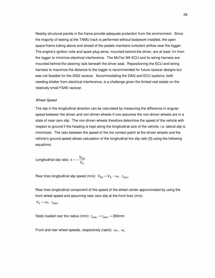
29

Nearby structural panels in the frame provide adequate protection from the environment. Since

the majority of testing at the TAMU track is performed without bodywork installed, the open

space-frame tubing above and ahead of the pedals maintains turbulent airflow near the logger.

The engine’s ignition coils and spark plug wires, mounted behind the driver, are at least 1m from

the logger to minimize electrical interference. The MoTec M4 ECU and its wiring harness are

mounted behind the steering rack beneath the driver seat. Repositioning the ECU and wiring

harness to maximize the distance to the logger is recommended for future racecar designs but

was not feasible for the 2002 racecar. Accommodating the DAQ and ECU systems, both

needing shelter from electrical interference, is a challenge given the limited real estate on the

relatively small FSAE racecar.

Wheel Speed

Tire slip in the longitudinal direction can be calculated by measuring the difference in angular

speed between the driven and non-driven wheels if one assumes the non-driven wheels are in a

state of near-zero slip. The non-driven wheels therefore determine the speed of the vehicle with

respect to ground if the heading is kept along the longitudinal axis of the vehicle, i.e. lateral slip is

minimized. The ratio between the speed of the tire contact patch at the driven wheels and the

vehicle’s ground speed allows calculation of the longitudinal tire slip ratio [5] using the following

equations:

Longitudinal slip ratio: X

SX

V

Vκ −=

Rear tires longitudinal slip speed (m/s): rstat,rXSX rωVV ⋅−=

Rear tires longitudinal component of the speed of the wheel center approximated by using the

front wheel speed and assuming near zero slip at the front tires (m/s):

stat,ffX rωV ⋅=

Static loaded rear tire radius (mm): 260mmrr stat,frstat, ==

Front and rear wheel speeds, respectively (rad/s): fω , rω

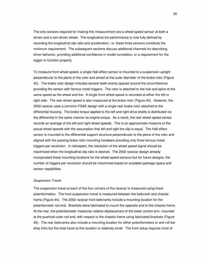
30

The only sensors required for making this measurement are a wheel speed sensor at both a

driven and a non-driven wheel. The longitudinal tire performance is now fully defined by

recording the longitudinal slip ratio and acceleration, i.e. these three sensors constitute the

minimum requirement. The subsequent sections discuss additional channels for describing

driver behavior, providing additional confidence in model correlation, or a requirement for the

logger to function properly.

To measure front wheel speed, a single Hall-effect sensor is mounted to a suspension upright

perpendicular to the plane of the rotor and aimed at the outer diameter of the brake rotor (Figure

42). The brake rotor design includes several teeth evenly spaced around the circumference

providing the sensor with ferrous metal triggers. The rotor is attached to the hub and spins at the

same speed as the wheel and tire. A single front wheel speed is recorded at either the left or

right side. The rear wheel speed is also measured at the brake rotor (Figure 43). However, the

2002 racecar uses a common FSAE design with a single rear brake rotor attached to the

differential housing. The brake torque applied to the left and right drive shafts is distributed via

the differential in the same manner as engine torque. As a result, the rear wheel speed sensor

records an average of the left and right wheel speeds. This is an approximate measure of the

actual wheel speeds with the assumption that left and right tire slip is equal. The Hall-effect

sensor is mounted to the differential support structure perpendicular to the plane of the rotor and

aligned with the passing brake rotor mounting hardware providing only three ferrous metal

triggers per revolution. In retrospect, the resolution of the wheel speed signal should be

maximized when the longitudinal slip ratio is desired. The 2002 racecar design already

incorporated these mounting locations for the wheel speed sensors but for future designs, the

number of triggers per revolution should be maximized based on available package space and

sensor capabilities.

Suspension Travel

The suspension travel at each of the four corners of the racecar is measured using linear

potentiometers. The front suspension travel is measured between the bellcrank and chassis

frame (Figure 44). The 2002 racecar front bellcranks include a mounting location for the

potentiometer rod end. Brackets were fabricated to mount the opposite end to the chassis frame.

At the rear, the potentiometer measures relative displacement of the lower control arm, mounted

at the pushrod outer rod end, with respect to the chassis frame using fabricated brackets (Figure

45). The rear bellcranks also include a mounting location for either potentiometers or anti-roll bar

drop links but the total travel at this location is relatively small. The front setup requires most of

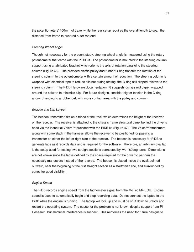
31

the potentiometers’ 100mm of travel while the rear setup requires the overall length to span the

distance from frame to pushrod outer rod end.

Steering Wheel Angle

Though not necessary for the present study, steering wheel angle is measured using the rotary

potentiometer that came with the PiDB kit. The potentiometer is mounted to the steering column

support using a fabricated bracket which orients the axis of rotation parallel to the steering

column (Figure 46). The provided plastic pulley and rubber O-ring transfer the rotation of the

steering column to the potentiometer with a certain amount of reduction. The steering column is

wrapped with electrical tape to reduce slip but during testing, the O-ring still slipped relative to the

steering column. The PiDB Hardware documentation [7] suggests using sand paper wrapped

around the column to minimize slip. For future designs, consider higher tension in the O-ring

and/or changing to a rubber belt with more contact area with the pulley and column.

Beacon and Lap Layout

The beacon transmitter sits on a tripod at the track which determines the height of the receiver

on the racecar. The receiver is attached to the chassis frame structural panel behind the driver’s

head via the industrial Velcro™ provided with the PiDB kit (Figure 47). The Velco™ attachment

along with some slack in the harness allows the receiver to be positioned for passing a

transmitter on either the left or right side of the racecar. The beacon is necessary for PiDB to

generate laps as it records data and is required for the software. Therefore, an arbitrary oval lap

is the setup used for testing: two straight sections connected by two 180deg turns. Dimensions

are not known since the lap is defined by the space required for the driver to perform the

necessary maneuvers instead of the reverse. The beacon is placed inside the oval, pointed

outward, near the beginning of the first straight section as a start/finish line, and surrounded by

cones for good visibility.

Engine Speed

The PiDB records engine speed from the tachometer signal from the MoTec M4 ECU. Engine

speed is used to automatically begin and stop recording data. Do not connect the laptop to the

PiDB while the engine is running. The laptop will lock up and must be shut down to unlock and

restart the operating system. The cause for the problem is not known despite support from Pi

Research, but electrical interference is suspect. This reinforces the need for future designs to

32

carefully consider placement of the ECU and DAQ systems as far from the engine as possible on

such a small racecar.

Throttle Position

The MoTec M4 ECU requires a TPS in order to determine control input to the engine. Since the

racecar already has a TPS installed, the PiDB borrows the signal from the MoTec wiring harness.

However, the 5V signal must be calibrated within the logger to relate position to voltage. The

calibration is generated using the output shown by MoTec relative to the TPS signal measured

with a voltmeter. The physical position of the throttle plate relative to sensor voltage was not

used because it could generate a difference between the recorded signals of the ECU and DAQ

system, particularly at part-throttle.

Sampling Rate

The sampling rates of all but the beacon receiver were set to 100Hz which provided a good

balance between signal representation and the limits of the logger 2MB memory card. PiDB

averages the wheel speed signal across several triggers from the Hall-effect sensor. The front

wheel speed sensor pointed at a 30-tooth trigger wheel (notches in the brake rotor) and produced

excellent resolution. However, the rear wheel speed sensor only had three triggers per revolution

forcing PiDB to wait longer between updates of the wheel speed signal. The effective update

rate for the rear wheel speed is about 10-15Hz as shown in Figure 48 using configuration 1 data

as an example. The rear wheel speed holds while the front wheel speed continues to increase.

As the front signal “catches up” with the rear signal, the calculated longitudinal slip ratio, also

shown in Figure 48, decreases rapidly between updates of the rear signal. The MoTec M4

tachometer signal logged by PiDB resulted in only 20Hz suggesting PiDB is performing an

average of tachometer signals as well. The acceleration, engine speed, and rear wheel speed

channels, particularly during a straight-line acceleration event of a FSAE racecar, rapidly change

at the beginning of the event and the 100Hz rate should be considered a minimum. For critical

channels, use higher sampling rates when the balance of memory card limit and track time

allows. Non-critical channels may be compromised if memory is a factor by reducing the

sampling rate on the lateral acceleration for example.

Miscellaneous DAQ System Suggestions

The PiDB kit purchased by TAMU FSAE contains the Pi DataBuddy MiniDash (Pi Research Part

No. 01K-163055-1) for displaying up to eight channels. The logger setup determines which

33

channels are available to the driver while on the track. During testing, the drivers had to estimate

the initial speed prior to beginning the straight-line acceleration event. In retrospect, the drivers

could improve consistency in initial speed if the MiniDash had been installed to display the

current wheel speed.

Potentiometers, speed sensors, thermocouples, or even strain gauges are all relatively

inexpensive when compared to the optical sensing equipment required for measuring tire slip.

Corrsys-Datron manufactures a series of non-contact optical sensors for this purpose. For

example, the CORREVIT® S-CE1 can measure the velocity vector with respect to ground,

providing an accurate representation of the longitudinal and lateral slip occurring at the tire

contact patch. The price is about two to three orders of magnitude above the Hall-effect sensors

and significantly outside the limit of funding for this study.

VEHICLE RESPONSE TESTING

The racecar is tested at the TAMU Riverside Campus which has a series of long runways. A

majority of the runway surface is cleared for racecar use but weeds growing between the seams

in the concrete mixed with a variety of debris create a wide range of grip. Several laps on the

same track setup helps clean the surface.

System Configurations

Recall, one of the objectives of the study is to validate the longitudinal performance of the full

vehicle model against the actual vehicle response recorded at the TAMU test track. Since the

rigid body model of the racecar’s kinematics is accurately characterized, the majority of error in

the simulated response is expected to arise from the Goodyear tire model representing the

Hoosier tire on the actual track surface. The dynamic inputs that affect the performance output

from the tire model, i.e. the longitudinal force, are normal load and slip ratio. Using two drivers

and the option of adding ballast, the resulting array of four configurations varies the static normal

load by 15% and the CG height, i.e. the longitudinal load transfer, by 2% (Table 9). The quantity

of ballast chosen is approximately equal to the difference in driver mass. As a result, two

configurations – light driver plus ballast and heavy driver without ballast – have nearly equal total

mass and only the overall CG location is changed.

1CORREVIT® Non-Contact Optical Sensors are manufactured by Corrsys-Datron of Wetzlar, Germany. Sensor

specifications available at http://www.corrsys-datron.com/optical_sensors.htm, [accessed June 2005].

34

The other two configurations – light driver without ballast and heavy driver with ballast – provide a

range of static load in addition to the change in CG location. The ballast mounts to the main roll

hoop support tubes directly over the rear suspension track width. The CG of the ballast is

located along the centerline of the vehicle at a height approximately equal to the top of the tire,

about 520mm above the ground.

Procedure

The following procedure outlines the general steps taken to measure the response of the 2002

TAMU FSAE racecar for each configuration:

1. Prior to arriving at the track.

a. DAQ system and laptop:

i. Calibrate sensors, set sampling rates, and configure logger as desired.

ii. Verify channel output in logger display.

iii. Memory card – clear and/or download any previous sessions from the logger.

iv. Charge laptop battery if necessary.

b. Vehicle:

i. Check fluid levels.

ii. Check tire pressures and set to 12psi.

iii. Check lug nut torque.

iv. Top off fuel tank if necessary.

v. Verify engine and MoTec are working properly.

vi. Adjust suspension for static corner weight, camber, and toe settings. For the present

study, the settings at static ride height with driver are: front and rear camber angles

vary from 0deg to -1deg, front toe overall 1.5mm out, rear toe varies from 5 to 6mm

in, and corner weights are equal within 1.4kg from left to right.

2. Prepare track, vehicle, and DAQ system while driver gets ready and belted in the seat.

a. Track:

i. Position beacon transmitter at the start of the first straight section of track, pointing

from inside the oval out so the beacon only crosses one portion of the track. The

driver should pass the beacon while still at a steady initial speed for the straight-line

acceleration event.

ii. Place cones at either end of the two straight sections of track to help the driver return

to the same locations for each lap.

b. DAQ system:

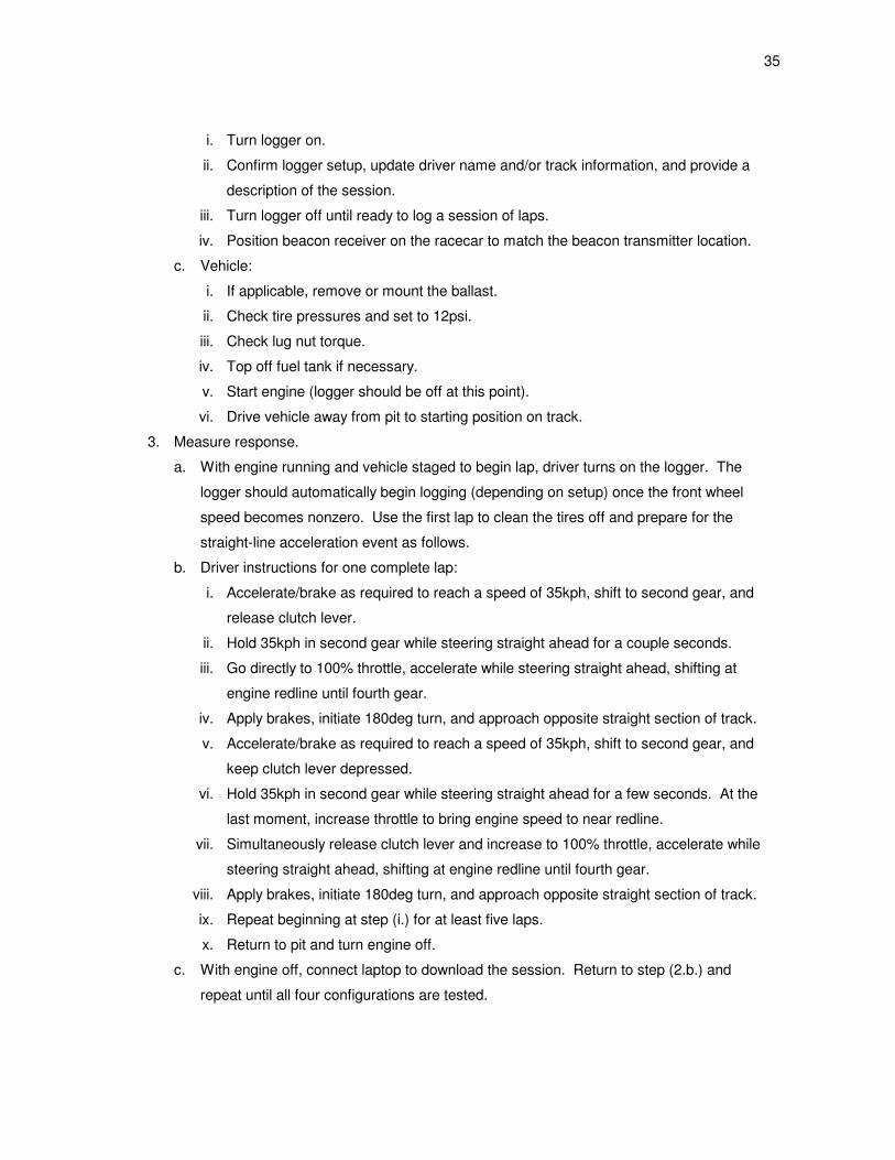
35

i. Turn logger on.

ii. Confirm logger setup, update driver name and/or track information, and provide a

description of the session.

iii. Turn logger off until ready to log a session of laps.

iv. Position beacon receiver on the racecar to match the beacon transmitter location.

c. Vehicle:

i. If applicable, remove or mount the ballast.

ii. Check tire pressures and set to 12psi.

iii. Check lug nut torque.

iv. Top off fuel tank if necessary.

v. Start engine (logger should be off at this point).

vi. Drive vehicle away from pit to starting position on track.

3. Measure response.

a. With engine running and vehicle staged to begin lap, driver turns on the logger. The

logger should automatically begin logging (depending on setup) once the front wheel

speed becomes nonzero. Use the first lap to clean the tires off and prepare for the

straight-line acceleration event as follows.

b. Driver instructions for one complete lap:

i. Accelerate/brake as required to reach a speed of 35kph, shift to second gear, and

release clutch lever.

ii. Hold 35kph in second gear while steering straight ahead for a couple seconds.

iii. Go directly to 100% throttle, accelerate while steering straight ahead, shifting at

engine redline until fourth gear.

iv. Apply brakes, initiate 180deg turn, and approach opposite straight section of track.

v. Accelerate/brake as required to reach a speed of 35kph, shift to second gear, and

keep clutch lever depressed.

vi. Hold 35kph in second gear while steering straight ahead for a few seconds. At the

last moment, increase throttle to bring engine speed to near redline.

vii. Simultaneously release clutch lever and increase to 100% throttle, accelerate while

steering straight ahead, shifting at engine redline until fourth gear.

viii. Apply brakes, initiate 180deg turn, and approach opposite straight section of track.

ix. Repeat beginning at step (i.) for at least five laps.

x. Return to pit and turn engine off.

c. With engine off, connect laptop to download the session. Return to step (2.b.) and

repeat until all four configurations are tested.

36

The lap contains two types of straight-line acceleration event. Both initially start in a rolling

condition at 35kph but one event begins with the clutch already engaged with the engine and the

other event begins as the driver releases the clutch pedal. The latter condition is closer to the

actual method in which the racecar is accelerated. However, the first case is appropriate for

correlating the model as it removes most if not all of the clutch effects in the overall response.

Plus, the racecar is not equipped with a tachometer and the drivers could not consistently start

the event at the same engine speed. This is possible if the PiDB MiniDash is utilized such as

was suggested for displaying wheel speed.

Running the event in second gear is selected to maximize use of the engine. The event begins

at around 5900rpm and concludes at engine redline, 13,500rpm. The drivers are instructed to

continue shifting and accelerating up to fourth gear to capture shift times. The model is capable

of shifting but the default settings are not typical of a sequentially shifted motorcycle engine, i.e.

the standard ACAR clutch and shifter inputs are about 2.0s while FSAE shifts require only 0.2s.

ADAMS/Driver, another software package working with ACAR, can control the full vehicle

simulation in a custom manner but is outside the scope of this study. Creating custom

ADAMS/Driver-controlled simulations is the next step towards predicting the racecar response

based on the recorded driver inputs at the track.

The track direction was not noted but was kept the same for all configurations. The testing was

performed in the following order:

1. 75kg driver – no ballast.

2. 75kg driver – with ballast.

3. 88kg driver – with ballast.

4. 88kg driver – no ballast.

Post-Processing

The data must be downloaded from the logger using the PiDB Logger Management software [8].

The PiDB Logger Management software is strictly for communicating with the logger and does

not offer any post-processing of the data. Once the data is on the laptop, the next step was

using the Pi Club Expert Analysis (CEA) software [10] supplied with the PiDB kit to view the data.

However, CEA does not offer the ability to export time history files for further analysis. It offers

the ability to view the data in histograms or with respect to a track map. The track map is

generated from the wheel speed channel ideally during an “easy” lap with very little tire slip. For

37

the present study, time history of the recorded responses is required to perform the necessary

analyses and plots. The Pi Version 6 software [11, 12] is able to view the files generated by the

PiDB Logger Management software and perform many more tasks than CEA. The most

important ability of V6 is exporting the data to a comma separated value file which can be used

by spreadsheet software, in this case Microsoft Excel.

Once the data is imported to a spreadsheet, the lap data is divided according to the two straight-

line acceleration events and the 180deg turn portions are removed. The events with the clutch

engaged prior to applying 100% throttle are extracted for further analysis. The lap time for each

event is adjusted such that t = 0s at the moment the longitudinal acceleration channel rapidly

increases. The suspension travel potentiometers were calibrated according to the travel

measured at the Risse Racing Jupiter-5 shock. To display the suspension travel as

displacement instead of position, the steady state shock position for each corner is used to

vertically shift the entire curve to zero. The same procedure is used with the ACAR simulated

response discussed later.

38

MODEL CORRELATION

The only parameter used in this study for adjusting the model to match the simulation results with

the measured system response is the scaling of the longitudinal tire model, i.e. DLON = BCDLON.

The scaling is equal to the ratio of peak recorded normalized longitudinal tire force FX/FZ to the

Goodyear tire model prediction of peak FX/FZ. Recall, the road coefficient of friction parameter in

the road data file is set to 1.0.

COMPARISON OF SIMULATED AND MEASURED RESPONSES

The following discussion refers to Figures 49-76, which show the results of both the ACAR and

measured responses for each configuration. The data presented are:

1. Longitudinal Acceleration vs. Time

a. Measured Response – longitudinal accelerometer channel from PiDB.

b. ACAR Response – chassis part longitudinal acceleration.

2. Engine Speed vs. Time

a. Measured Response – tachometer signal from MoTec M4 ECU; channel logged by PiDB,

filtered.

b. ACAR Response – powertrain subsystem engine speed.

3. Longitudinal Chassis Speed vs. Time

a. Measured Response – front wheel speed channel from PiDB; assumes constant tire

radius of 260mm.

b. ACAR Response – chassis part longitudinal speed.

4. Longitudinal Slip Ratio vs. Time

a. Measured Response – calculated with front and rear wheel speeds from PiDB; assumes

constant tire radius of 260mm, filtered.

b. ACAR Response – calculated slip between rear tire and road surface; tire radius based

on Goodyear tire model vertical stiffness and applied normal load.

5. Normalized Tire Force vs. Longitudinal Slip Ratio

a. Measured Response – calculated with longitudinal accelerometer from PiDB, vehicle CG

location, and vehicle geometry; assumes constant tire radius of 260mm.

b. ACAR Response – calculated using longitudinal and normal loads on tire; tire radius

based on Goodyear tire model vertical stiffness and applied normal load.

6. Throttle Position

a. Measured Response – throttle positions channel from PiDB.

39

b. ACAR Response – driver input to powertrain subsystem.

7. Damper Travel

a. Measured Response – damper position channels from PiDB; vertical shift places steady

state position at zero.

b. ACAR Response – damper length; vertical shift places steady state length at zero.

For all but the normalized longitudinal tire force, the measured response data is from a single

straight-line acceleration event that the driver obtained the most precise initial vehicle speed.

The plots of tire force as a function of slip ratio present all the available measured response data

for each particular configuration.

Configuration 1

Figures 49-55 show the measured vehicle responses and the ACAR simulated responses for

configuration 1, light driver without ballast. The Goodyear tire model scaled to 78% (DLON =

BCDLON = 0.78) results in the upper limit, for this configuration, of the recorded normalized

longitudinal tire force FX/FZ (Figure 53).

Configuration 2


configuration 2, heavy driver without ballast. Note the initial speed is only 32kph for this

configuration (Figure 58). The ACAR model in this instance was simulated with a 32kph initial

speed to match the recorded data, which did not include an event with 35kph initial speed. The

Goodyear tire model is scaled to both 78% and 75% for this configuration. The 78% curve

appears beyond the upper limit for this set of events and the 75% curve represents grip near the

recorded tire performance as shown by the peak slip (Figures 59-60).

Configuration 3


configuration 3, light driver with ballast. The Goodyear tire model is scaled to 78% for this

configuration to provide good correlation overall.

Configuration 4


configuration 4, heavy driver with ballast. The Goodyear tire model is scaled to 72% for this

40

configuration to provide good correlation with the recorded tire performance (Figures 73-74). The

slip ratio predicted by ACAR at DLON = 72% remains above the recorded slip ratio at t = 0.5-1.0s

indicating the level of grip is changing (Figure 73). The road surface at different locations along

the track or heat building up in the tire are two examples of why grip would change during the

event.

Overall Observations

Predicted longitudinal acceleration during about the first 0.3s of all the simulations is consistently

high compared to the measured response. Recall the engine torque map in the model is based

on dynamometer measurements of the 2004 engine. The difference between the 2004 and 2002

racecars both in track performance and driver impressions confirm a significant lack of initial

torque in the 2002 engine. This difference in torque is apparent in the transient response of the

dampers where the model consistently predicts larger displacements.

The measured longitudinal acceleration lags the throttle control input by about 0.05-0.10s. The

predicted response from ACAR shows longitudinal acceleration of the chassis part tracking TPS

with virtually no lag indicating there is some inertia not modeled in the templates. One

explanation involves the transport inertia within the engine intake system. The intake system

uses a single inlet providing air to a plenum that distributes air to the four combustion chambers

via runners to each cylinder. The combustion chamber does not respond to TPS input until

pressure within the intake plenum increases and the required restriction [1] on the inlet limits this

fill rate. The engine speed at the beginning of the straight-line acceleration event is about

6,000rpm (100Hz), i.e. each revolution of the crankshaft requires 0.01s. It is entirely possible the

plenum could take about 5 revolutions of the crankshaft in order to respond to a 100% TPS input

from a near-idle condition. Also, the response time would be compounded by the transient

performance of the ECU such as poor tuning of the acceleration enrichment.

Before modifying the model to include the inertia, minimize the response time in the 2002 engine.

Tune the ECU with the 2002 engine on the dynamometer while addressing transient control

parameters in addition to the baseline fuel and ignition maps. The objective is to match the 2002

engine performance with recent FSAE engines and accurately measure the torque output.

Several combinations of TPS and speed are required for tuning the fuel and ignition maps.

Recording torque output with the dynamometer at each TPS/speed position will add significant

detail to the engine model improving prediction of part-throttle behavior in future simulations.

Validate the changes using PiDB, which can log the MAP signal from the MoTec M4 ECU, and

41

quantify the time required to fill the plenum. If the measured response time continues to differ

significantly from the simulation, the powertrain subsystem would need an additional DOF

describing the transport inertia behavior.

CONCLUSIONS

The results of the study indicate the range of on-track longitudinal tire behavior for the Hoosier

tire is about 75±3% of the Goodyear tire model. Though the correlation procedure fixed the road

surface coefficient of friction while varying the tire model parameters, the reverse would result in

the same longitudinal vehicle response. The peak available grip between tire and road is

determined by the product of µ x DLON. Therefore, the study does not differentiate between tire

performance and road surface performance – the results instead describe the interface between

tire and road. If subsequent use of the model assumes the interface applies to both longitudinal

and lateral behavior, then the next logical step is to evaluate the model accuracy in predicting

lateral or combined lateral/longitudinal behavior. This is achieved by one of two configurations:

• DLAT = DLON = 75±3% with µ = 100%.

• DLAT = DLON = 100% with µ = 75±3%.

Recall, the scaling of the tire “stiffness” factor, BCDLON, does not affect peak tire performance.

Though BCDLON was scaled the same as DLON throughout this study, comparison of initial slope

in Figures 13, 53, 60, 67, and 74 supports the claim that the overall vehicle response is

significantly less sensitive to changes in the stiffness factor, BCD, than changes in the peak

factor, D. In turn, the configuration with the tire parameters kept at 100% and the road surface

reduced to 75±3% is a fair assumption given the results of this study. However, confidence in

this assumption requires significantly more data describing the vehicle response with lateral slip

maneuvers, e.g. constant radius acceleration event (a.k.a. skid pad), slalom, or complete

autocross course.

42

RECOMMENDED NEXT STEPS

Using the results and suggestions of this study, the full vehicle ACAR model has potential as a

valuable analysis tool for the FSAE racecar design process. Next steps, in order of

recommended priority, include:

1. Improve 2002 engine performance and ACAR model powertrain subsystem correlation using

the dynamometer to tune the ECU and record an accurate torque map. Measure the MAP

signal during a straight-line acceleration event to quantify the intake plenum fill rate.

2. Apply tire model scaling instead to the road surface coefficient of friction and validate overall

vehicle dynamics against maneuvers with lateral slip, e.g. constant radius acceleration event.

3. Add refinement to powertrain subsystem:

a. Expanding the engine torque map to cover part-throttle conditions.

b. Modify the templates to include a DOF between the driver input, TPS, and the engine

model to describe transport behavior in the intake system.

4. Expand use of ACAR’s simulation capabilities:

a. Utilize the many other standard simulation events (note – braking parameters need to be

defined at this stage if braking events will be simulated).

b. Develop custom driver control files (.dcf) or use ADAMS/Driver to apply the same

controls measured at the track to the model.

43

SUMMARY

The objective of the study was to create a full vehicle dynamics model of the 2002 TAMU FSAE

racecar using ACAR and validate the model’s longitudinal performance against recorded vehicle

responses using a DAQ system. The process of achieving this objective involved:

1. Repairing the 2002 racecar.

2. Measuring the vehicle mass, estimating inertias, and measuring geometry in order to

populate the ACAR model database.

3. Testing the Risse Racing Jupiter-5 shocks to define the sub-model stiffness and damping

properties.

4. Installing the Pi DataBuddy data acquisition system on the 2002 racecar.

5. Testing the racecar and recording the response in a longitudinal acceleration event at the

TAMU Riverside Campus.

6. Correlate the ACAR simulation results to match the measured response via scaling the

Goodyear tire model to represent the Hoosier tire on-track performance.

The most significant deliverable from this study is a working full vehicle ACAR model which

allows future vehicle dynamic analysis. In a close second, the installed and working PiDB DAQ

system helps provide the detailed feedback from the track which is missing from the present

FSAE design process.

The results of the correlation process have shown that the dynamometer results for the 2004

engine predict higher performance than the measured response of the 2002 engine. This

observation from the data is confirmed by driver impressions and comparison to the 2004

racecar performance. An engine torque map generated from the dynamometer measurements

for the as-installed 2002 engine setup is necessary for eliminating this error.

The Hoosier tire on the TAMU Riverside Campus track surface is 75±3% of the predicted peak

longitudinal tire performance by the Goodyear tire model combined with a road surface friction

coefficient of 1.0.

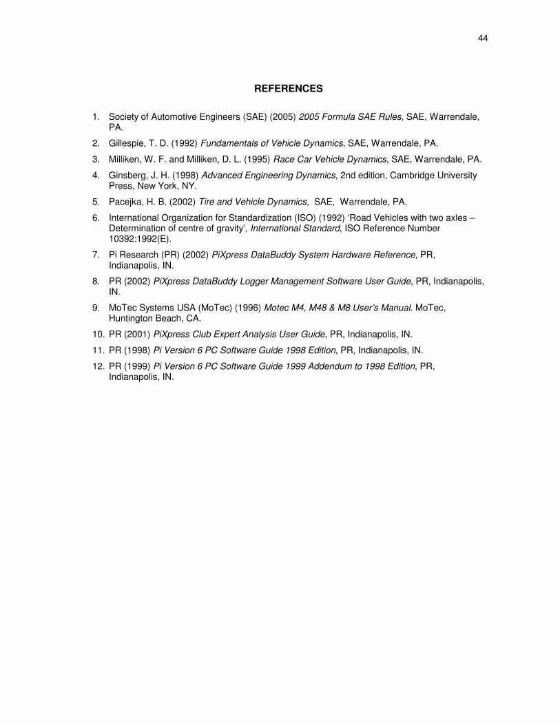
44

REFERENCES

1. Society of Automotive Engineers (SAE) (2005) 2005 Formula SAE Rules, SAE, Warrendale, PA.

2. Gillespie, T. D. (1992) Fundamentals of Vehicle Dynamics, SAE, Warrendale, PA.

3. Milliken, W. F. and Milliken, D. L. (1995) Race Car Vehicle Dynamics, SAE, Warrendale, PA.

4. Ginsberg, J. H. (1998) Advanced Engineering Dynamics, 2nd edition, Cambridge University Press, New York, NY.

5. Pacejka, H. B. (2002) Tire and Vehicle Dynamics, SAE, Warrendale, PA.

6. International Organization for Standardization (ISO) (1992) ‘Road Vehicles with two axles – Determination of centre of gravity’, International Standard, ISO Reference Number 10392:1992(E).

7. Pi Research (PR) (2002) PiXpress DataBuddy System Hardware Reference, PR, Indianapolis, IN.

8. PR (2002) PiXpress DataBuddy Logger Management Software User Guide, PR, Indianapolis, IN.

9. MoTec Systems USA (MoTec) (1996) Motec M4, M48 & M8 User’s Manual. MoTec, Huntington Beach, CA.

10. PR (2001) PiXpress Club Expert Analysis User Guide, PR, Indianapolis, IN.

11. PR (1998) Pi Version 6 PC Software Guide 1998 Edition, PR, Indianapolis, IN.

12. PR (1999) Pi Version 6 PC Software Guide 1999 Addendum to 1998 Edition, PR, Indianapolis, IN.

45

APPENDIX A

FIGURES

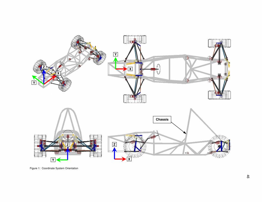
46

Figure 1: Coordinate System Orientation

Z

Y

Z

X

Y

X

Y

X

Z

Chassis

47

Figure 2: Front Suspension Subsystem

Y X

Z

Z

Y

Z

X

Y

X

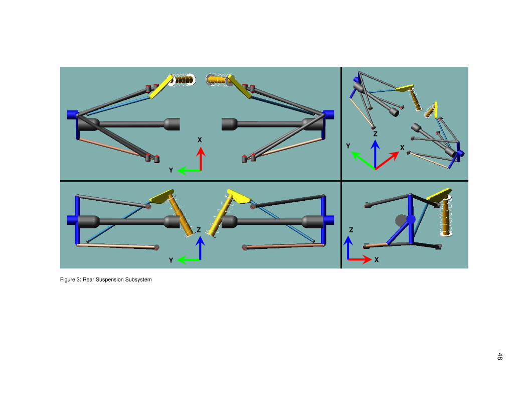
48

Figure 3: Rear Suspension Subsystem

Y X

Z

Z

Y

Z

X

Y

X

49

Figure 4: Front Suspension Subsystem Parts

Figure 5: Rear Suspension Subsystem Parts

bellcrank

damper_bellcrank

arb_bushing_mount (not shown)

damper_chassis

uca

prod

tierod

upright

hub

lca

damper_bellcrank

bellcrank

damper_chassis

prod

tripot

drive_shaft

uca

spindle

lca

upright

tierod

arb_bushing_mount (not shown)

50

Figure 6: Anti-Roll Bar Subsystem Parts

Figure 7: Steering Subsystem Parts

droplink

arb_bushing_mount (defined within the suspension subsystem)

arb

steering_wheel steering_column_support steering_column intermediate_shaft steering_shaft pinion rack_housing steering_rack

51

Figure 8: Coil-Over Shock Sub-Model

0

2000

4000

6000

8000

10000

12000

0 20 40 60 80

Displacement (mm)

Sp

ring

Forc

e (

N)

Front Coil Spring &Gas ChargeStiffness

Front Limit ofTravel, Transitionto Bump Stop

Estimate of FrontElastomer "BumpStop"

Rear Coil Spring &Gas ChargeStiffness

Rear Limit ofTravel, Transitionto Bump Stop

Estimate of RearElastomer "BumpStop"

Unloaded (free) length:

Front = 209mm

Rear = 216mm

Figure 9: Suspension Springs

bellcrank

prod

damper_chassis

damper_bellcrank spring (not a part)

shock_to_chassis hardpoint

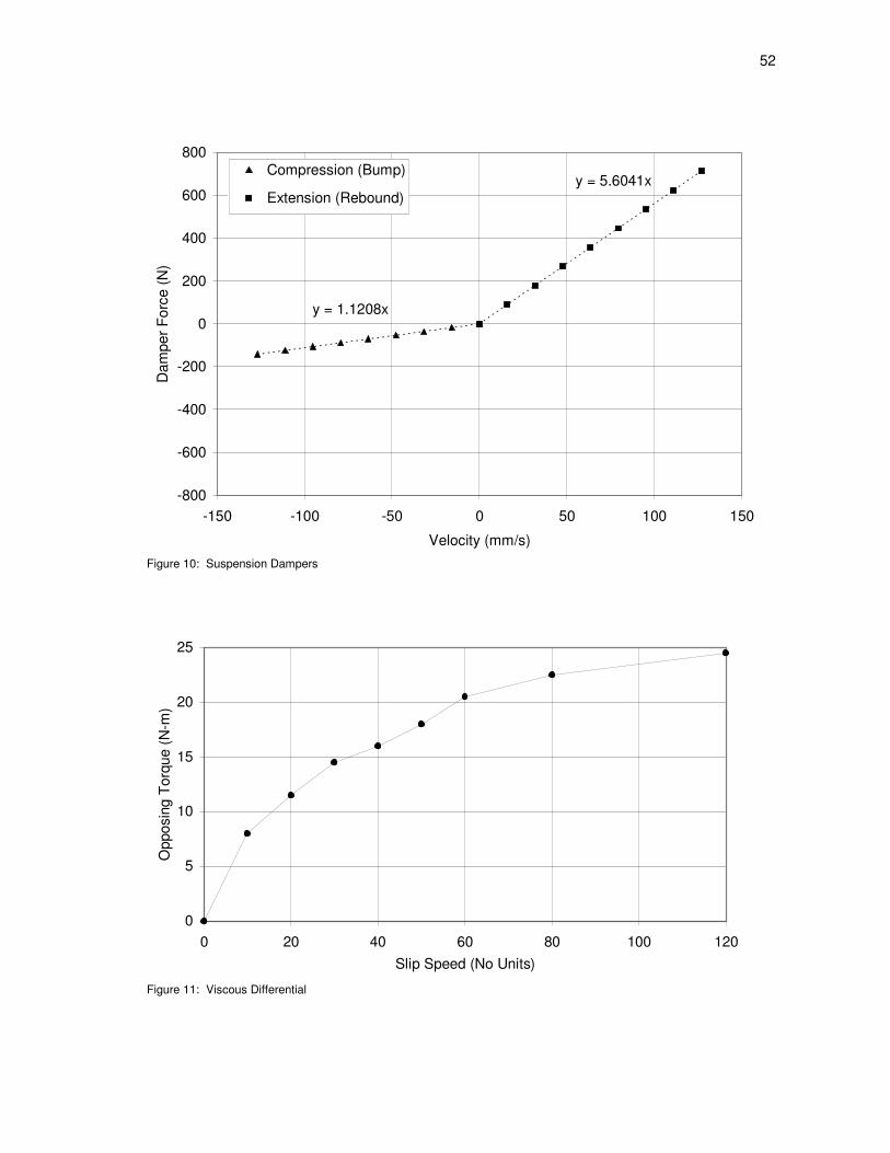
52

y = 1.1208x

y = 5.6041x

-800

-600

-400

-200

0

200

400

600

800

-150 -100 -50 0 50 100 150

Velocity (mm/s)

Da

mpe

r F

orc

e (

N)

Compression (Bump)

Extension (Rebound)

Figure 10: Suspension Dampers

0

5

10

15

20

25

0 20 40 60 80 100 120

Slip Speed (No Units)

Opposin

g T

orq

ue (

N-m

)

Figure 11: Viscous Differential

53

1.2

1.3

1.4

1.5

1.6

0 5 10 15 20 25 30 35 40

Longitudinal Slip Ratio (%)

Norm

aliz

ed L

ong.

Tire F

orc

e (

FX

/FZ

)

DLON = BCDLON = 100% (FZ = -0.67kN)



Figure 12: Normal Load Effects on Normalized Longitudinal Tire Force (Goodyear FSAE Tire Model, 20in outside diameter, 6.5in width, 13in diameter rim, 12psi inflation pressure)

0.6

0.7

0.8

0.9

1.0

1.1

1.2

1.3

1.4

1.5

1.6

0 5 10 15 20 25 30 35 40


Norm

aliz

ed L

ong.

Tire F

orc

e (

FX

/FZ

)




Figure 13: Scaling Effects on Normalized Longitudinal Tire Force (Goodyear FSAE Tire Model, 20in outside diameter, 6.5in width, 13in diameter rim, 12psi inflation pressure)

54

Figure 14: Simulation Setup – Full-Vehicle Analysis Straight-Line Acceleration

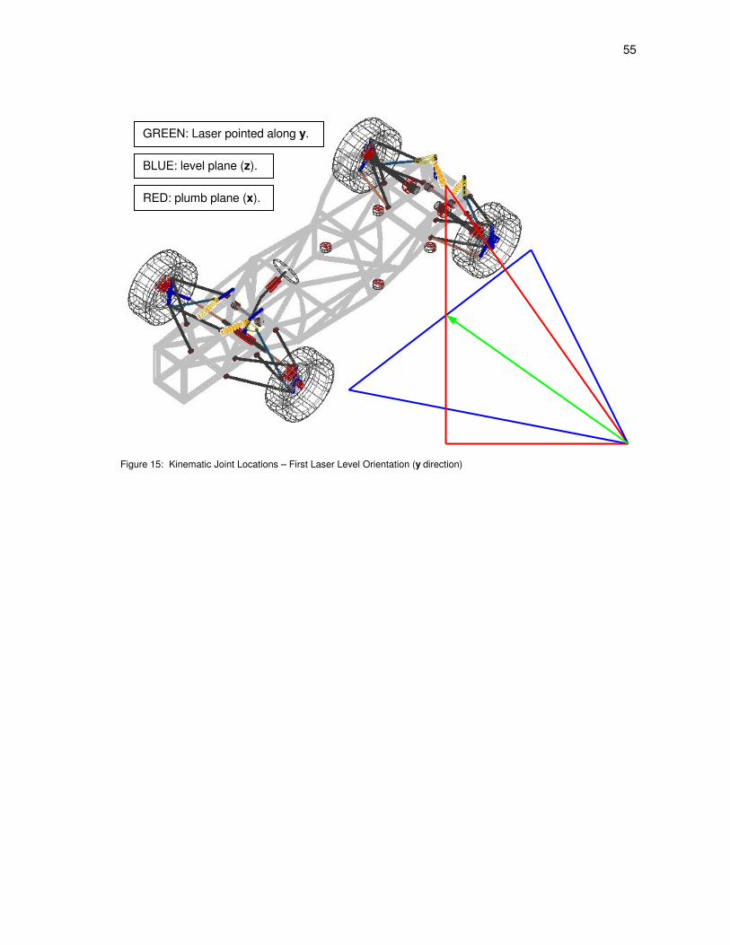
55

Figure 15: Kinematic Joint Locations – First Laser Level Orientation (y direction)

GREEN: Laser pointed along y.

BLUE: level plane (z).

RED: plumb plane (x).

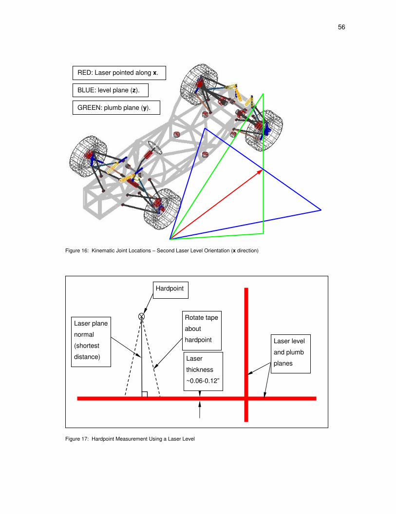
56

Figure 16: Kinematic Joint Locations – Second Laser Level Orientation (x direction)

Figure 17: Hardpoint Measurement Using a Laser Level

Hardpoint

Laser plane

normal

(shortest

distance)

Rotate tape

about

hardpoint Laser level

and plumb

planes Laser

thickness

~0.06-0.12”

RED: Laser pointed along x.

BLUE: level plane (z).

GREEN: plumb plane (y).

57

1. Solid model drawing of 2002 frame. 2. Simplified geometry of driver. 3. Simplified geometry of powertrain part. 4. Simplified geometry of ballast.

Figure 18: SolidWorks Model for Estimating Inertia

1

3

4

2

58

-0.1 -0.2 -0.3 -0.7 -1.0 -1.4 -1.7 -2.0 -2.4 -2.7 -3.1 -3.4 -3.7 -4.1 -4.4 -4.7 -5.1 -5.4 -5.5 -5.5 -5.5 -5.5 -5.5 -5.5 -5.5

10.0

15.0

18.0

23.0

27.0

30.0

35.033.0

30.0

25.0

35.2

38.9

42.1

46.0

50.7 51.1

47.446.2

45.044.0

41.038.639.5

52.152.3

-10

-5

0

5

10

15

20

25

30

35

40

45

50

55

60

20

00

30

00

40

00

50

00

60

00

70

00

80

00

90

00

10

00

0

11

00

0

12

00

0

13

00

0

14

00

0

15

00

0

Engine Speed (rev/min)

En

gin

e T

orq

ue

(N

-m)

Estimated Engine RetardingTorque (TPS = 0%)

Estimated Torque at speedsbelow dyno results (TPS = 100%)

Estimated Torque at speedsabove dyno results (TPS = 100%)

Measured Dyno Torque for 2004FSAE Engine with "Long" Runners(TPS = 100%)

Figure 19: Powertrain Subsystem Engine Torque Map

59

-1500

-1200

-900

-600

-300

0

300

600

900

1200

1500

-150 -100 -50 0 50 100 150

Speed (mm/s)

Shock F

orc

e (

N)

B mid/R mid

B mid/R hi

B mid/R lo

B hi/R mid

B lo/R mid

Figure 20: Risse Racing Jupiter-5 Shock #1 – Total Force, All 5 Tested Settings

60

y = 5.7276x + 79.801

y = 2.324x + 84.363

y = 1.1082x - 113.08

y = 7.4275x - 180.11

-1500

-1200

-900

-600

-300

0

300

600

900

1200

1500

-150 -125 -100 -75 -50 -25 0 25 50 75 100 125 150Speed (mm/s)

Shock D

am

pin

g F

orc

e (

N)

Rebound (0 to 13 mm)

Bump (13 to 0 mm)

Bump (0 to -13 mm)

Rebound (-13 to 0 mm)

Figure 21: Risse Racing Jupiter-5 Shock #1 – Damping, MID Bump + MID Rebound

y = 7.6353x + 313.77

y = 10.729x - 76.986y = 3.3475x + 166.85

y = 1.1286x - 130.9

-1500

-1200

-900

-600

-300

0

300

600

900

1200

1500

-150 -125 -100 -75 -50 -25 0 25 50 75 100 125 150Speed (mm/s)

Shock D

am

pin

g F

orc

e (

N)


Bump (13 to 0 mm)

Bump (0 to -13 mm)


Figure 22: Risse Racing Jupiter-5 Shock #1 – Damping, MID Bump + HI Rebound

61

y = 4.7022x + 88.276

y = 6.48x - 177.48

y = 2.2243x + 80.791

y = 0.9867x - 119.01

-1500

-1200

-900

-600

-300

0

300

600

900

1200

1500

-150 -125 -100 -75 -50 -25 0 25 50 75 100 125 150Speed (mm/s)

Shock D

am

pin

g F

orc

e (

N)


Bump (13 to 0 mm)

Bump (0 to -13 mm)


Figure 23: Risse Racing Jupiter-5 Shock #1 – Damping, MID Bump + LOW Rebound

y = 4.5761x + 96.199

y = 7.4102x - 280.53

y = 8.5104x + 217.7

y = 2.8891x - 483.42

-1500

-1200

-900

-600

-300

0

300

600

900

1200

1500

-150 -125 -100 -75 -50 -25 0 25 50 75 100 125 150Speed (mm/s)

Shock D

am

pin

g F

orc

e (

N)


Bump (13 to 0 mm)

Bump (0 to -13 mm)


Figure 24: Risse Racing Jupiter-5 Shock #1 – Damping, HI Bump + MID Rebound

62

y = 4.8461x + 96.211

y = 6.6153x - 171.5

y = 1.705x + 67.722

y = 0.5408x - 123.7

-1500

-1200

-900

-600

-300

0

300

600

900

1200

1500

-150 -125 -100 -75 -50 -25 0 25 50 75 100 125 150Speed (mm/s)

Shock D

am

pin

g F

orc

e (

N)


Bump (13 to 0 mm)

Bump (0 to -13 mm)


Figure 25: Risse Racing Jupiter-5 Shock #1 – Damping, LOW Bump + MID Rebound

y = 2.0951x + 161.55

y = 2.062x + 164.75

y = 2.2779x + 203.39

60

80

100

120

140

160

180

200

220

240

260

-15 -10 -5 0 5 10 15Displacement (mm)

Shock S

tiff

ness F

orc

e (

N)


Bump (13 to -13 mm)


Figure 26: Risse Racing Jupiter-5 Shock #1 – Stiffness (Speed = 0.13 mm/s)

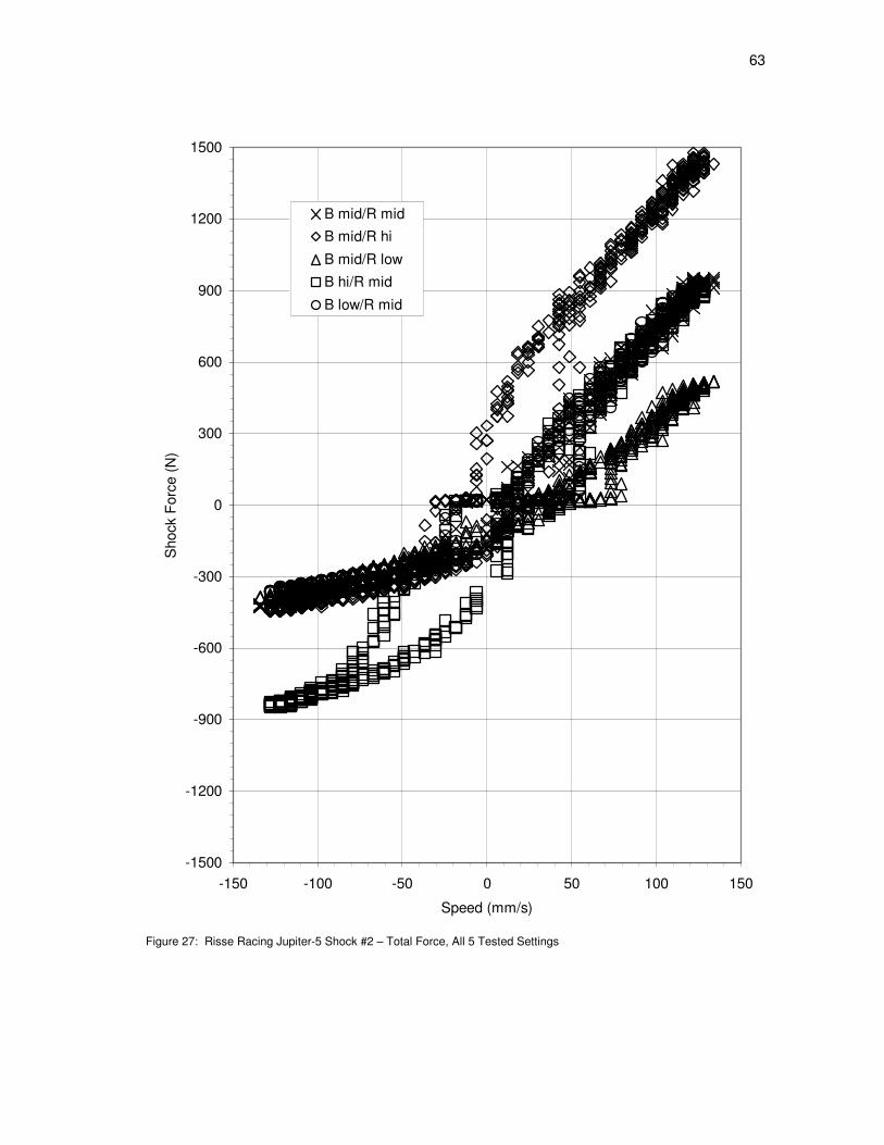
63

-1500

-1200

-900

-600

-300

0

300

600

900

1200

1500

-150 -100 -50 0 50 100 150

Speed (mm/s)

Shock F

orc

e (

N)

B mid/R mid

B mid/R hi

B mid/R low

B hi/R mid

B low/R mid


64

y = 7.5734x + 106.46

y = 9.423x - 152.45y = 2.9241x + 77.409

y = 1.5515x - 103.44

-1500

-1200

-900

-600

-300

0

300

600

900

1200

1500

-150 -125 -100 -75 -50 -25 0 25 50 75 100 125 150Speed (mm/s)

Shock D

am

pin

g F

orc

e (

N)


Bump (13 to 0 mm)

Bump (0 to -13 mm)



y = 8.1349x + 544.33

y = 13.027x - 1.3299y = 4.0382x + 166.78

y = 1.5382x - 126.3

-1500

-1200

-900

-600

-300

0

300

600

900

1200

1500

-150 -125 -100 -75 -50 -25 0 25 50 75 100 125 150Speed (mm/s)

Shock D

am

pin

g F

orc

e (

N)


Bump (13 to 0 mm)

Bump (0 to -13 mm)



65

y = 4.5914x + 20.969

y = 5.6925x - 143.62

y = 2.2595x + 43.78

y = 1.5233x - 74.616

-1500

-1200

-900

-600

-300

0

300

600

900

1200

1500

-150 -125 -100 -75 -50 -25 0 25 50 75 100 125 150Speed (mm/s)

Shock D

am

pin

g F

orc

e (

N)


Bump (13 to 0 mm)

Bump (0 to -13 mm)



y = 7.5157x + 95.849

y = 9.9977x - 214.56

y = 7.4768x + 158.39

y = 3.0758x - 350.14

-1500

-1200

-900

-600

-300

0

300

600

900

1200

1500

-150 -125 -100 -75 -50 -25 0 25 50 75 100 125 150Speed (mm/s)

Shock D

am

pin

g F

orc

e (

N)


Bump (13 to 0 mm)

Bump (0 to -13 mm)



66

y = 7.6648x + 95.303

y = 9.4787x - 154.66

y = 2.4374x + 65.453

y = 1.1009x - 103.64

-1500

-1200

-900

-600

-300

0

300

600

900

1200

1500

-150 -125 -100 -75 -50 -25 0 25 50 75 100 125 150Speed (mm/s)

Shock D

am

pin

g F

orc

e (

N)


Bump (13 to 0 mm)

Bump (0 to -13 mm)



y = 0.8772x + 103.06y = 0.9746x + 101.45

y = 1.5604x + 138.2

60

80

100

120

140

160

180

200

220

240

260

-15 -10 -5 0 5 10 15Displacement (mm)

Shock S

tiff

ness F

orc

e (

N)


Bump (13 to -13 mm)



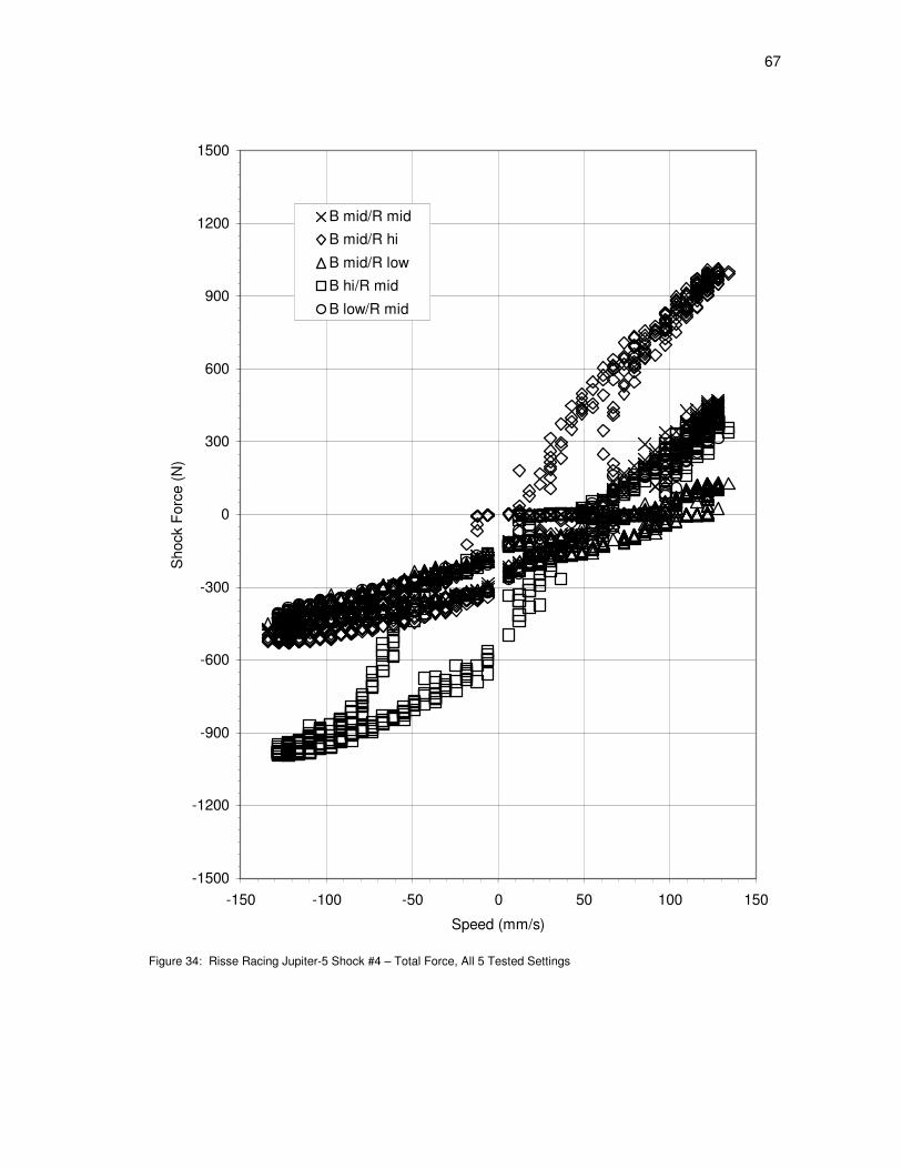
67

-1500

-1200

-900

-600

-300

0

300

600

900

1200

1500

-150 -100 -50 0 50 100 150

Speed (mm/s)

Shock F

orc

e (

N)

B mid/R mid

B mid/R hi

B mid/R low

B hi/R mid

B low/R mid


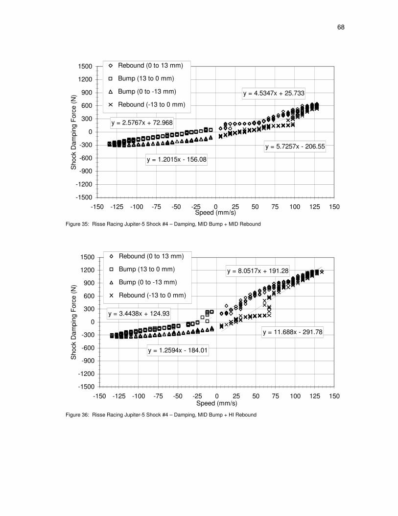
68

y = 4.5347x + 25.733

y = 5.7257x - 206.55

y = 2.5767x + 72.968

y = 1.2015x - 156.08

-1500

-1200

-900

-600

-300

0

300

600

900

1200

1500

-150 -125 -100 -75 -50 -25 0 25 50 75 100 125 150Speed (mm/s)

Shock D

am

pin

g F

orc

e (

N)


Bump (13 to 0 mm)

Bump (0 to -13 mm)



y = 8.0517x + 191.28

y = 11.688x - 291.78

y = 3.4438x + 124.93

y = 1.2594x - 184.01

-1500

-1200

-900

-600

-300

0

300

600

900

1200

1500

-150 -125 -100 -75 -50 -25 0 25 50 75 100 125 150Speed (mm/s)

Shock D

am

pin

g F

orc

e (

N)


Bump (13 to 0 mm)

Bump (0 to -13 mm)



69

y = 1.9761x + 43.793

y = 2.7794x - 137.43

y = 2.3769x + 87.089

y = 0.9377x - 145.18

-1500

-1200

-900

-600

-300

0

300

600

900

1200

1500

-150 -125 -100 -75 -50 -25 0 25 50 75 100 125 150Speed (mm/s)

Shock D

am

pin

g F

orc

e (

N)


Bump (13 to 0 mm)

Bump (0 to -13 mm)



y = 3.8946x + 39.802

y = 6.233x - 300.73

y = 7.8486x + 167.6

y = 2.8563x - 460.3

-1500

-1200

-900

-600

-300

0

300

600

900

1200

1500

-150 -125 -100 -75 -50 -25 0 25 50 75 100 125 150Speed (mm/s)

Shock D

am

pin

g F

orc

e (

N)


Bump (13 to 0 mm)

Bump (0 to -13 mm)



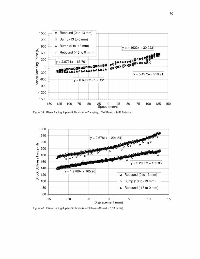
70

y = 4.1622x + 30.923

y = 5.4975x - 210.91

y = 2.0791x + 63.701

y = 0.6953x - 163.22

-1500

-1200

-900

-600

-300

0

300

600

900

1200

1500

-150 -125 -100 -75 -50 -25 0 25 50 75 100 125 150Speed (mm/s)

Shock D

am

pin

g F

orc

e (

N)


Bump (13 to 0 mm)

Bump (0 to -13 mm)



y = 2.2082x + 165.86

y = 1.9789x + 165.96

y = 2.6781x + 204.84

60

80

100

120

140

160

180

200

220

240

260

-15 -10 -5 0 5 10 15Displacement (mm)

Shock S

tiff

ness F

orc

e (

N)


Bump (13 to -13 mm)



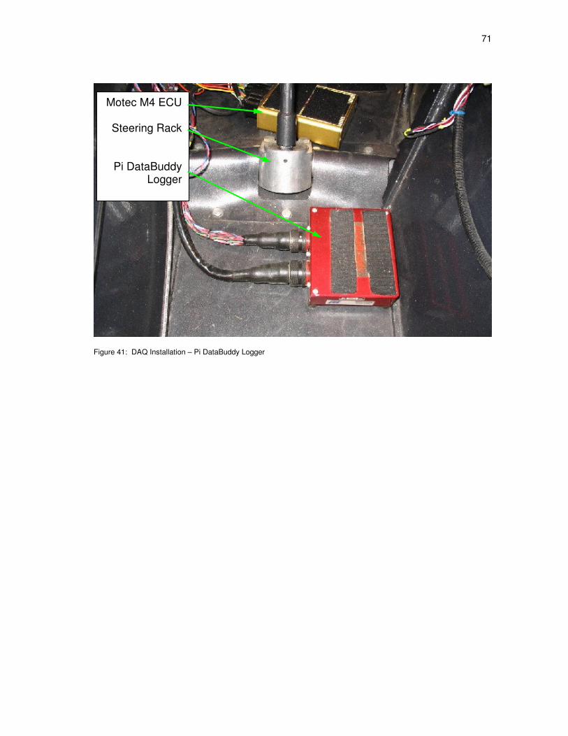
71

Figure 41: DAQ Installation – Pi DataBuddy Logger

Motec M4 ECU

Steering Rack

Pi DataBuddy Logger

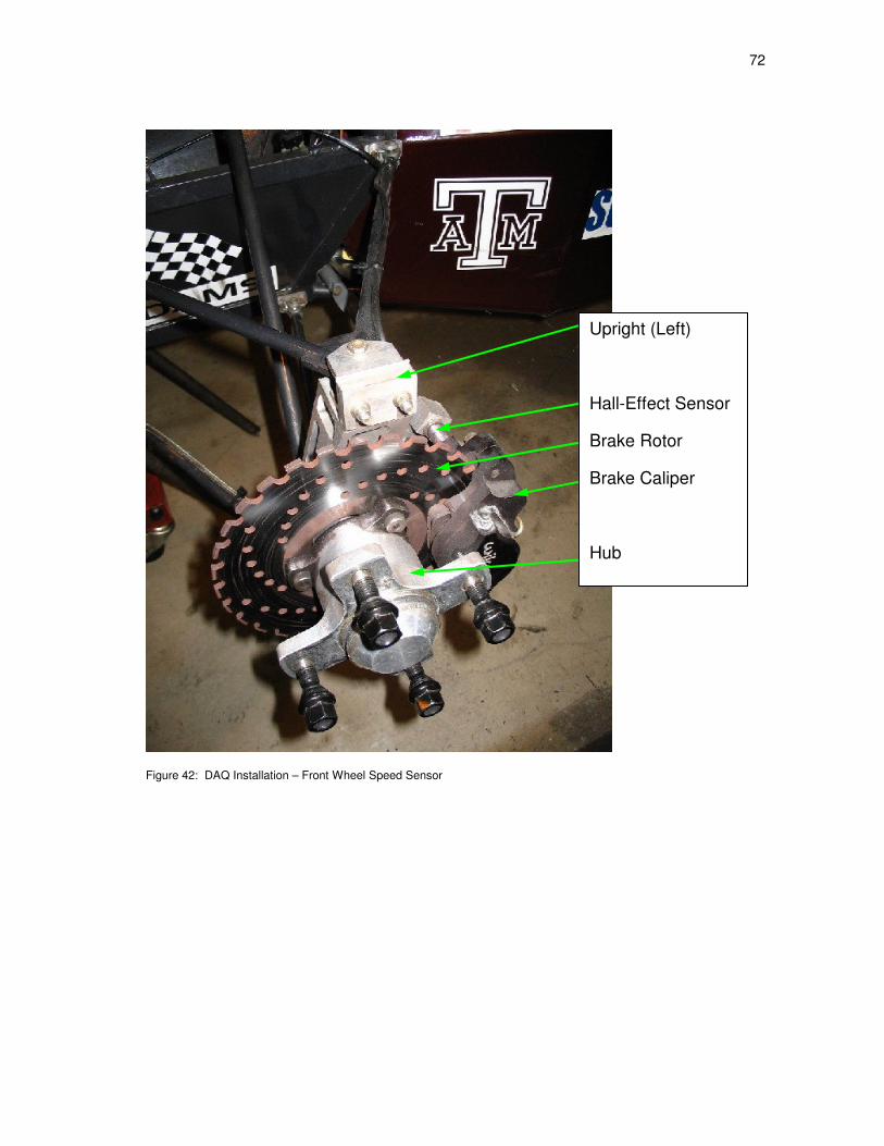
72

Figure 42: DAQ Installation – Front Wheel Speed Sensor

Upright (Left)

Hall-Effect Sensor

Brake Rotor

Brake Caliper

Hub

73

Figure 43: DAQ Installation – Rear Wheel Speed Sensor

Chain Drive

Brake Rotor

Hall-Effect Sensor

Brake Rotor Hardware (1 of 3)

Differential Housing

Tripod (Right)

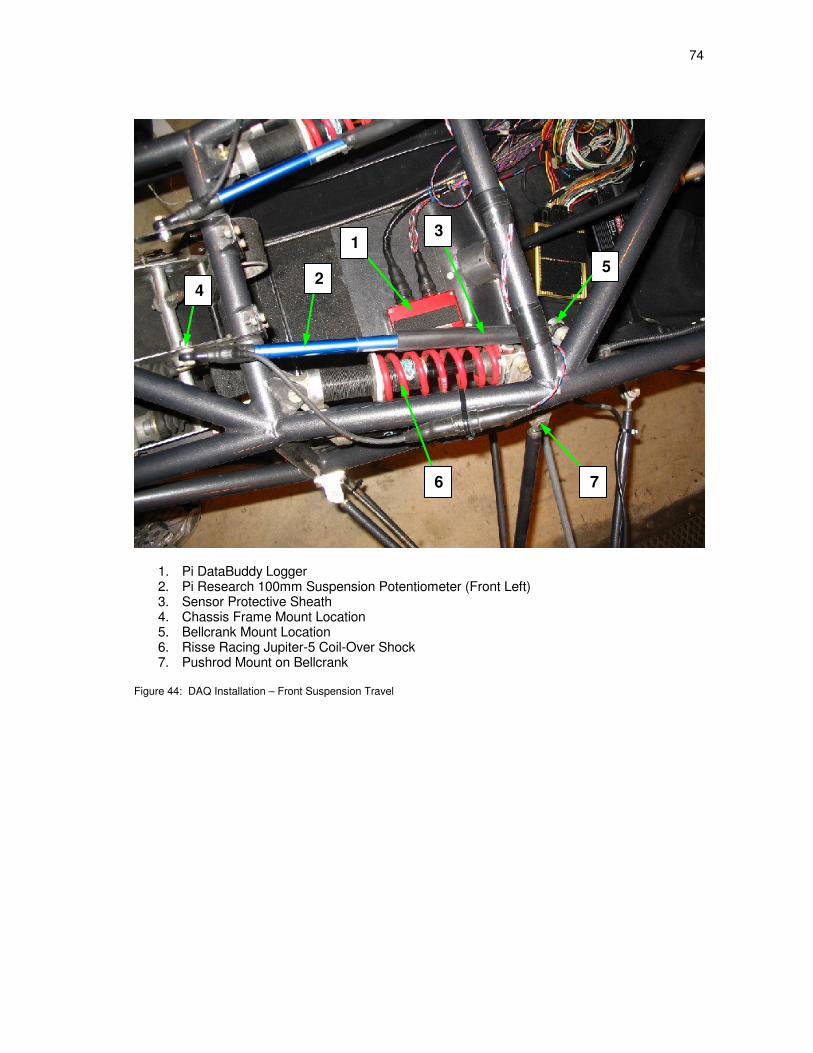
74

1. Pi DataBuddy Logger 2. Pi Research 100mm Suspension Potentiometer (Front Left) 3. Sensor Protective Sheath 4. Chassis Frame Mount Location 5. Bellcrank Mount Location 6. Risse Racing Jupiter-5 Coil-Over Shock 7. Pushrod Mount on Bellcrank

Figure 44: DAQ Installation – Front Suspension Travel

4

5 2

1

6 7

3

75

1. Pi Research 100mm Suspension Potentiometer (Rear Right) 2. Sensor Protective Sheath 3. Chassis Frame Mount Location 4. Lower Control Arm Mount Location 5. Pushrod 6. Bellcrank 7. Upright 8. Lower Control Arm

Figure 45: DAQ Installation – Rear Suspension Travel

4

2

1

6

3

5

7

8

76

Figure 46: DAQ Installation – Steering Wheel Angle

Figure 47: DAQ Installation – Beacon Receiver

Back of Instrument Panel

Rotary Pot. Pulley (O-Ring not shown)

Steering Column

Steering Wheel

Main Roll Hoop

Receiver

Head Restraint

77

0

5

10

15

20

25

30

35

40

45

50

55

60

65

70

75

80

0.00 0.25 0.50 0.75 1.00 1.25 1.50 1.75 2.00

Time (s)

Rear

Wheel S

peed (

km

/hr)

and L

ongitudin

al S

lip R

atio (

%)

Rear Wheel Speed Sampled at100Hz (km/hr)

Rear Wheel Speed filtered atPiDB Update Rate (km/hr)

Slip Ratio - Rear Wheel Speedsampled at 100Hz (%)

Slip Ratio - Rear Wheel Speedfiltered at PiDB update rate (%)

Figure 48: Configuration 1 – Filtered Rear Wheel Speed and Longitudinal Slip Ratio

78

0.0

0.1

0.2

0.3

0.4

0.5

0.6

0.7

0.8

0.9

1.0

0.00 0.25 0.50 0.75 1.00 1.25 1.50 1.75 2.00

Time (s)

Longitudin

al A

ccele

ration (

G)

Measured Response

ACAR Response, DLON = BCDLON = 78%

Figure 49: Configuration 1 – Longitudinal Chassis Acceleration

4000

5000

6000

7000

8000

9000

10000

11000

12000

13000

14000

0.00 0.25 0.50 0.75 1.00 1.25 1.50 1.75 2.00

Time (s)

Engin

e S

peed (

rev/m

in)

Measured Response


Figure 50: Configuration 1 – Engine Speed

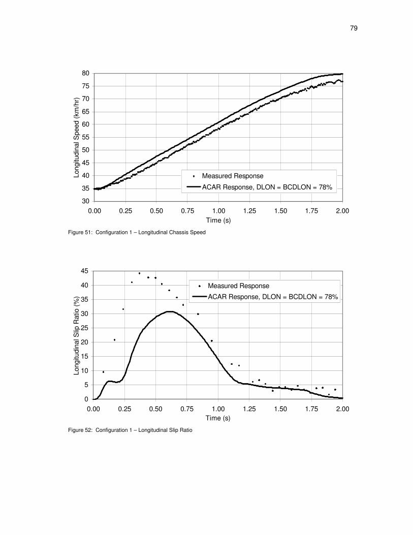
79

30

35

40

45

50

55

60

65

70

75

80

0.00 0.25 0.50 0.75 1.00 1.25 1.50 1.75 2.00

Time (s)

Longitudin

al S

peed (

km

/hr)

Measured Response


Figure 51: Configuration 1 – Longitudinal Chassis Speed

0

5

10

15

20

25

30

35

40

45

0.00 0.25 0.50 0.75 1.00 1.25 1.50 1.75 2.00

Time (s)

Longitudin

al S

lip R

atio (

%)

Measured Response


Figure 52: Configuration 1 – Longitudinal Slip Ratio

80

0.0

0.2

0.4

0.6

0.8

1.0

1.2

1.4

0 5 10 15 20 25 30 35 40 45


Norm

aliz

ed T

ire F

orc

e (

Fx/F

z)

Measured Response


Figure 53: Configuration 1 – Normalized Tire Force vs. Longitudinal Slip Ratio

0

10

20

30

40

50

60

70

80

90

100

110

-0.25 -0.20 -0.15 -0.10 -0.05 0.00 0.05 0.10 0.15 0.20 0.25

Time (s)

Thro

ttle

Positio

n (

%)

Measured Response

ACAR Response, DLON =BCDLON = 78%

Figure 54: Configuration 1 – Throttle Position

81

-10

-8

-6

-4

-2

0

2

4

6

8

10

0.00 0.25 0.50 0.75 1.00 1.25 1.50 1.75 2.00

Time (s)

Dam

per

Tra

vel (m

m)

MeasuredLeft Front

MeasuredRight Front

MeasuredLeft Rear

MeasuredRight Rear

ACAR-Front,DLON =BCDLON =78%

ACAR-Rear,DLON =BCDLON =78%

Figure 55: Configuration 1 – Damper Travel

82

0.0

0.1

0.2

0.3

0.4

0.5

0.6

0.7

0.8

0.9

1.0

0.00 0.25 0.50 0.75 1.00 1.25 1.50 1.75 2.00Time (s)

Longitudin

al A

ccele

ration (

G)

Measured Response




4000

5000

6000

7000

8000

9000

10000

11000

12000

13000

14000

0.00 0.25 0.50 0.75 1.00 1.25 1.50 1.75 2.00Time (s)

Engin

e S

peed (

rev/m

in)

Measured Response




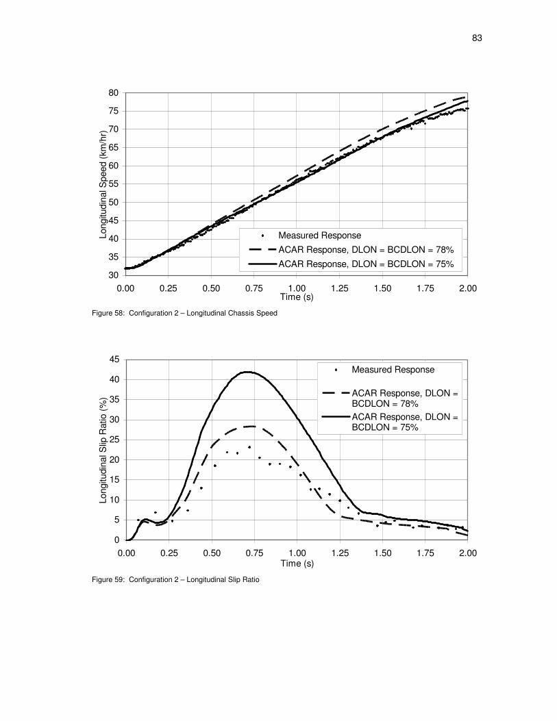
83

30

35

40

45

50

55

60

65

70

75

80

0.00 0.25 0.50 0.75 1.00 1.25 1.50 1.75 2.00Time (s)

Longitudin

al S

peed (

km

/hr)

Measured Response




0

5

10

15

20

25

30

35

40

45

0.00 0.25 0.50 0.75 1.00 1.25 1.50 1.75 2.00Time (s)

Longitudin

al S

lip R

atio (

%)

Measured Response




84

0.0

0.2

0.4

0.6

0.8

1.0

1.2

1.4

0 5 10 15 20 25 30 35 40 45 50 55


Norm

aliz

ed T

ire F

orc

e (

Fx/F

z)

Measured Response




0

10

20

30

40

50

60

70

80

90

100

110

-0.25 -0.20 -0.15 -0.10 -0.05 0.00 0.05 0.10 0.15 0.20 0.25

Time (s)

Thro

ttle

Positio

n (

%)

Measured Response



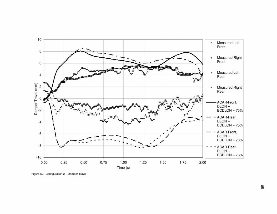
85

-10

-8

-6

-4

-2

0

2

4

6

8

10

0.00 0.25 0.50 0.75 1.00 1.25 1.50 1.75 2.00

Time (s)

Dam

per

Tra

vel (m

m)

Measured LeftFront

Measured RightFront

Measured LeftRear

Measured RightRear

ACAR-Front,DLON =BCDLON = 75%

ACAR-Rear,DLON =BCDLON = 75%

ACAR-Front,DLON =BCDLON = 78%

ACAR-Rear,DLON =BCDLON = 78%


86

0.0

0.1

0.2

0.3

0.4

0.5

0.6

0.7

0.8

0.9

1.0

0.00 0.25 0.50 0.75 1.00 1.25 1.50 1.75 2.00Time (s)

Longitudin

al A

ccele

ration (

G)

Measured Response



4000

5000

6000

7000

8000

9000

10000

11000

12000

13000

14000

0.00 0.25 0.50 0.75 1.00 1.25 1.50 1.75 2.00

Time (s)

Engin

e S

peed (

rev/m

in)

Measured Response



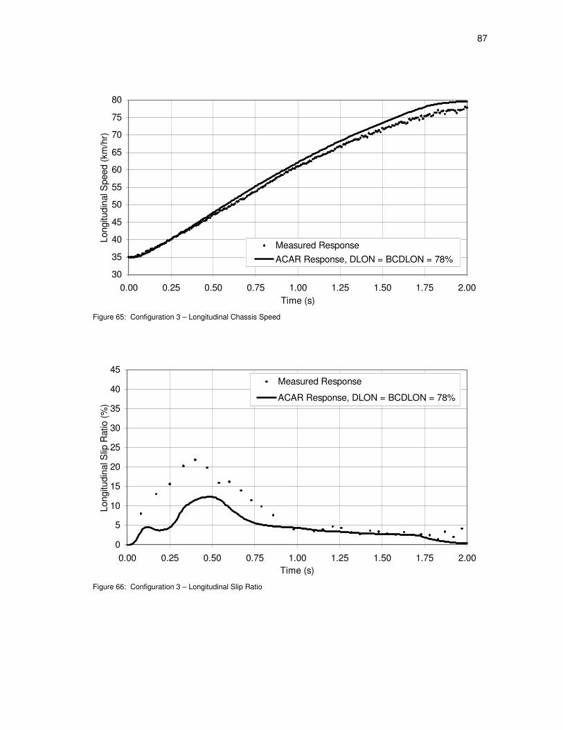
87

30

35

40

45

50

55

60

65

70

75

80

0.00 0.25 0.50 0.75 1.00 1.25 1.50 1.75 2.00

Time (s)

Longitudin

al S

peed (

km

/hr)

Measured Response



0

5

10

15

20

25

30

35

40

45

0.00 0.25 0.50 0.75 1.00 1.25 1.50 1.75 2.00

Time (s)

Longitudin

al S

lip R

atio (

%)

Measured Response



88

0.0

0.2

0.4

0.6

0.8

1.0

1.2

1.4

0 5 10 15 20 25 30 35 40 45


Norm

aliz

ed T

ire F

orc

e (

Fx/F

z)

Measured Response



0

10

20

30

40

50

60

70

80

90

100

110

-0.25 -0.20 -0.15 -0.10 -0.05 0.00 0.05 0.10 0.15 0.20 0.25

Time (s)

Thro

ttle

Positio

n (

%)

Measured Response



89

-10

-8

-6

-4

-2

0

2

4

6

8

10

0.00 0.25 0.50 0.75 1.00 1.25 1.50 1.75 2.00

Time (s)

Dam

per

Tra

vel (m

m)

MeasuredLeft Front

MeasuredRight Front

MeasuredLeft Rear

MeasuredRight Rear




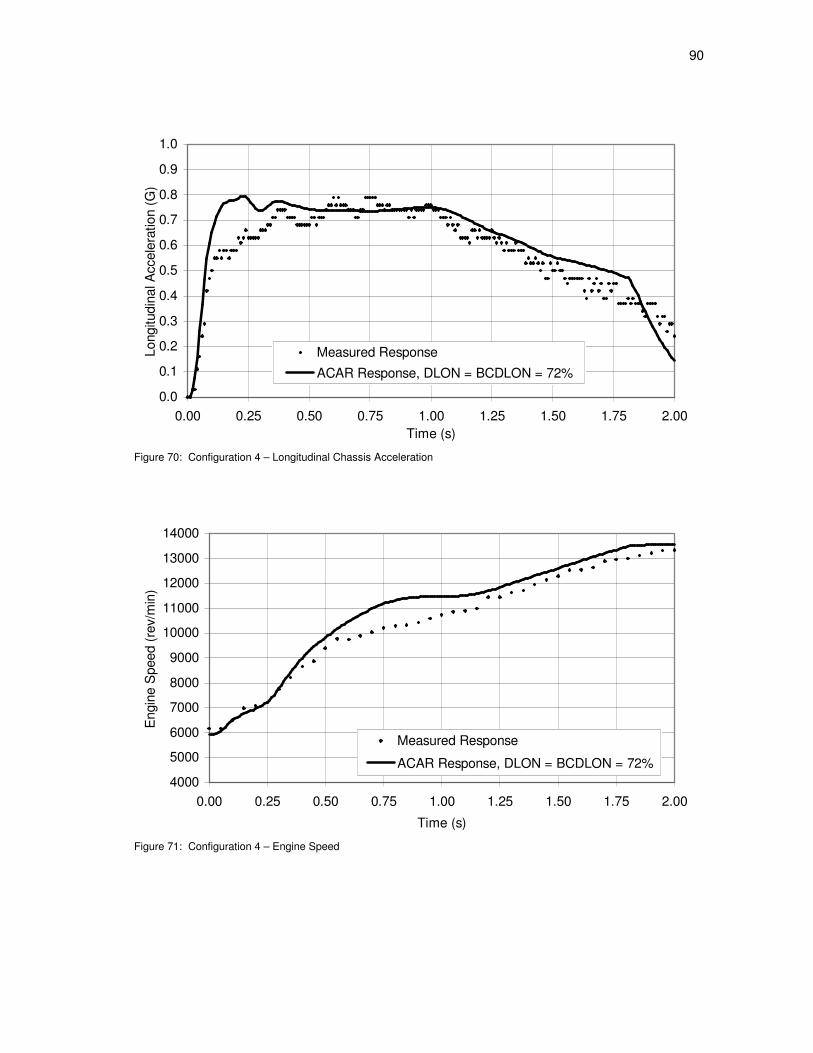
90

0.0

0.1

0.2

0.3

0.4

0.5

0.6

0.7

0.8

0.9

1.0

0.00 0.25 0.50 0.75 1.00 1.25 1.50 1.75 2.00

Time (s)

Longitudin

al A

ccele

ration (

G)

Measured Response



4000

5000

6000

7000

8000

9000

10000

11000

12000

13000

14000

0.00 0.25 0.50 0.75 1.00 1.25 1.50 1.75 2.00

Time (s)

Engin

e S

peed (

rev/m

in)

Measured Response



91

30

35

40

45

50

55

60

65

70

75

80

0.00 0.25 0.50 0.75 1.00 1.25 1.50 1.75 2.00

Time (s)

Longitudin

al S

peed (

km

/hr)

Measured Response



0

5

10

15

20

25

30

35

40

45

0.00 0.25 0.50 0.75 1.00 1.25 1.50 1.75 2.00

Time (s)

Longitudin

al S

lip R

atio (

%)

Measured Response



92

0.0

0.2

0.4

0.6

0.8

1.0

1.2

1.4

0 5 10 15 20 25 30 35 40 45


Norm

aliz

ed T

ire F

orc

e (

Fx/F

z)

Measured Response



0

10

20

30

40

50

60

70

80

90

100

110

-0.25 -0.20 -0.15 -0.10 -0.05 0.00 0.05 0.10 0.15 0.20 0.25

Time (s)

Thro

ttle

Positio

n (

%)

Measured Response



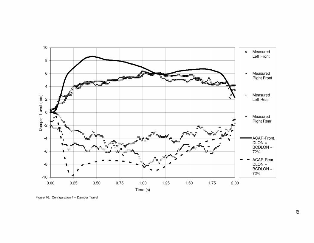
93

-10

-8

-6

-4

-2

0

2

4

6

8

10

0.00 0.25 0.50 0.75 1.00 1.25 1.50 1.75 2.00

Time (s)

Dam

per

Tra

vel (m

m)

MeasuredLeft Front

MeasuredRight Front

MeasuredLeft Rear

MeasuredRight Rear




94

APPENDIX B

TABLES

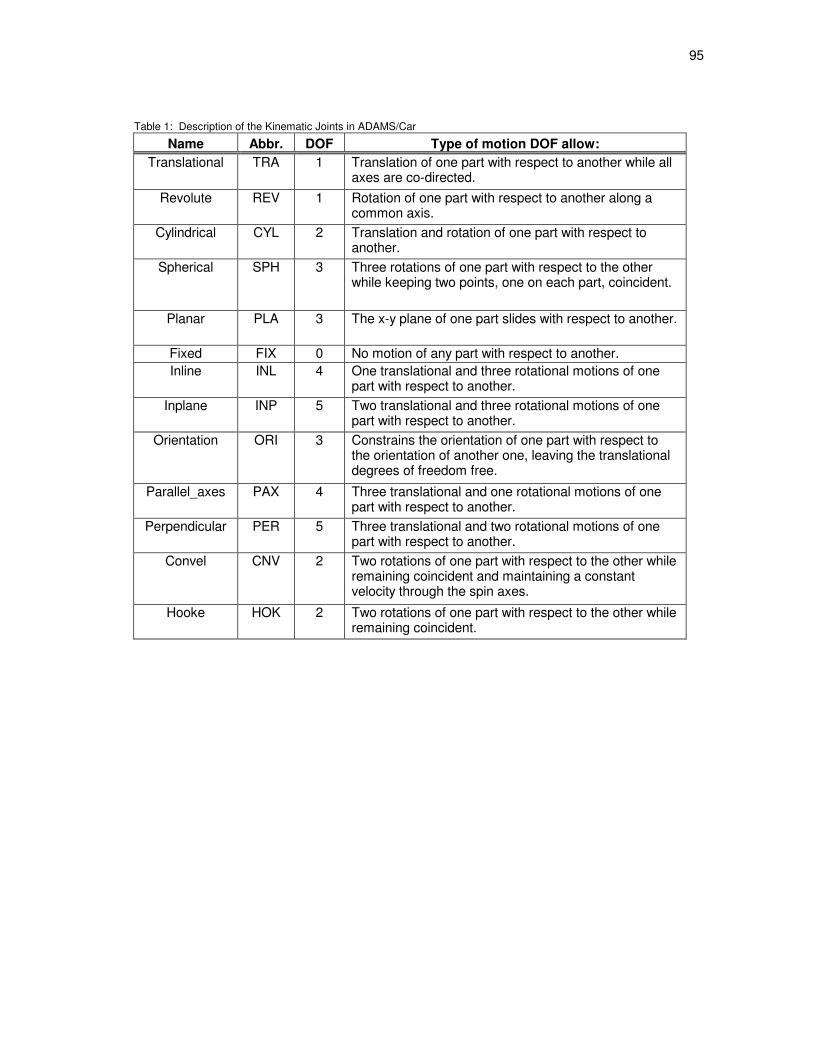
95

Table 1: Description of the Kinematic Joints in ADAMS/Car

Name Abbr. DOF Type of motion DOF allow:

Translational TRA 1 Translation of one part with respect to another while all axes are co-directed.

Revolute REV 1 Rotation of one part with respect to another along a common axis.

Cylindrical CYL 2 Translation and rotation of one part with respect to another.

Spherical SPH 3 Three rotations of one part with respect to the other while keeping two points, one on each part, coincident.

Planar PLA 3 The x-y plane of one part slides with respect to another.

Fixed FIX 0 No motion of any part with respect to another.

Inline INL 4 One translational and three rotational motions of one part with respect to another.

Inplane INP 5 Two translational and three rotational motions of one part with respect to another.

Orientation ORI 3 Constrains the orientation of one part with respect to the orientation of another one, leaving the translational degrees of freedom free.

Parallel_axes PAX 4 Three translational and one rotational motions of one part with respect to another.

Perpendicular PER 5 Three translational and two rotational motions of one part with respect to another.

Convel CNV 2 Two rotations of one part with respect to the other while remaining coincident and maintaining a constant velocity through the spin axes.

Hooke HOK 2 Two rotations of one part with respect to the other while remaining coincident.

96

Table 2: Hardpoint Definitions

Item Hardpoint Joint Part 1 Part 2

No. I.D. Name Type Name Name


1 A2 arblink_to_bellcrank SPH bellcrank droplink (Front ARB Sub.)

2 A3 arb_bushing_mount FIX arb_bushing_mount chassis (Chassis Sub.)

3 A4 bellcrank_pivot REV bellcrank chassis (Chassis Sub.)

4 A5 bellcrank_pivot_orient Defines bellcrank_pivot REV joint axis of rotation.

5 A6 lca_front BUS lca chassis (Chassis Sub.)

6 A7 lca_outer SPH lca upright

7 A8 lca_rear BUS lca chassis (Chassis Sub.)

8 A9 prod_outer SPH prod lca

9 A10 prod_to_bellcrank HOK prod bellcrank

10 A11 shock_to_bellcrank HOK damper_bellcrank bellcrank

11 A11, A12 relative coordinates CYL damper_bellcrank damper_chassis

12 A12 shock_to_chassis HOK damper_chassis chassis (Chassis Sub.)

13 A13 tierod_inner HOK tierod steering_rack (Steering Sub.)

14 A14 tierod_outer SPH tierod lca

15 A15 uca_front BUS uca chassis (Chassis Sub.)

16 A16 uca_outer SPH uca upright

17 A17 uca_rear BUS uca chassis (Chassis Sub.)

18 A18 wheel_center REV hub upright

97

Table 2: Continued




19 B2 arblink_to_bellcrank SPH bellcrank droplink (Rear ARB Sub.)

20 B3 arb_bushing_mount FIX arb_bushing_mount chassis (Chassis Sub.)

21 B4 bellcrank_pivot REV bellcrank chassis (Chassis Sub.)

22 B5 bellcrank_pivot_orient Defines bellcrank_pivot REV joint axis of rotation.

23 B6 drive_shaft_inr TRA tripot diff_output (Powertrain Sub.)

24 CNV tripot drive_shaft

25 B7 lca_front BUS lca chassis (Chassis Sub.)

26 B8 lca_outer SPH lca upright

27 B9 lca_rear BUS lca chassis (Chassis Sub.)

28 B10 prod_outer SPH prod lca

29 B11 prod_to_bellcrank HOK prod bellcrank

30 B12 shock_to_bellcrank HOK damper_bellcrank bellcrank

31 B12, B13 relative coordinates CYL damper_bellcrank damper_chassis

32 B13 shock_to_chassis HOK damper_chassis chassis (Chassis Sub.)

33 B14 tierod_inner HOK tierod chassis (Chassis Sub.)

34 B15 tierod_outer SPH tierod lca

35 B16 uca_front BUS uca chassis (Chassis Sub.)

36 B17 uca_outer SPH uca upright

37 B18 uca_rear BUS uca chassis (Chassis Sub.)

38 B19 wheel_center REV spindle upright

39 CNV spindle drive_shaft

98

Table 2: Continued



Steering Subsystem

40 C1 intermediate_shaft_forward HOK steering_shaft intermediate_shaft

41 C2 intermediate_shaft_rear HOK intermediate_shaft steering_column

42 C3 pinion_center_at_rack REV pinion rack_housing

43 FIX pinion steering_shaft

44 CPL pinion (rotation DOF) steering_rack (translation DOF)

45 C4 steeringwheel_center FIX steering_column steering_wheel

46 C2, C4 relative coordinates CYL steering_column steering_column_support

47 C2, C4 relative coordinates FIX steering_column_support chassis (Chassis Sub.)

48 A13 relative coordinates TRA steering_rack rack_housing

49 A13 relative coordinates FIX rack_housing chassis (Chassis Sub.)


50 D1 front_engine_mount BUS powertrain chassis (Chassis Sub.)

51 D2 rear_engine_mount BUS powertrain chassis (Chassis Sub.)

52 B6 relative coordinates REV powertrain diff_output

Front ARB Subsystem

53 E1 arb_middle REV arb (left) arb (right)

54 E2 arb_bend Defines location of bend in arb (connects "middle" to "droplink")

55 E3 arb_bushing BUS

arb arb_bushing_mount (Front Susp. Sub.)

56 E4 droplink_to_arb HOK arb droplink

99

Table 2: Continued



Rear ARB Subsystem

57 F1 arb_middle REV arb (left) arb (right)

58 F2 arb_bend Defines location of bend in arb (connects "middle" to "droplink")

59 F3 arb_bushing BUS

arb arb_bushing_mount (Rear Susp. Sub.)

60 F4 droplink_to_arb HOK arb droplink

Front Tires Subsystem

61 A18 wheel_center FIX wheel hub (Front Susp. Sub.)

Rear Tires Subsystem

62 B19 wheel_center FIX wheel spindle (Rear Susp. Sub.)

100

Table 3: Part Mass and Inertia

Item Part Symmetry Mass Inertia (kg-mm2)

No. Name (kg) IXX IYY IZZ

Front Suspension Subsystem Total Mass = 1.06E+01

1 arb_bushing_mount left/right 4.50E-02 2.93E-01 2.93E-01 2.93E-01

2 bellcrank left/right 2.55E-01 1.76E+02 1.29E+02 1.46E+02

3 damper_bellcrank left/right 1.13E-01 2.93E+02 2.93E+02 1.76E+02

4 damper_chassis left/right 2.27E-01 5.85E+02 5.85E+02 2.93E+02

5 hub left/right 1.90E+00 5.85E+03 5.85E+03 8.78E+03

6 lca left/right 4.54E-01 7.84E+03 3.69E+03 1.15E+04

7 prod left/right 1.98E-01 3.19E+03 3.19E+03 4.39E+00

8 tierod left/right 1.70E-01 1.46E+03 1.46E+03 3.80E+00

9 uca left/right 3.69E-01 4.68E+03 5.12E+03 9.74E+03

10 upright left/right 1.56E+00 5.36E+03 2.34E+03 5.56E+03

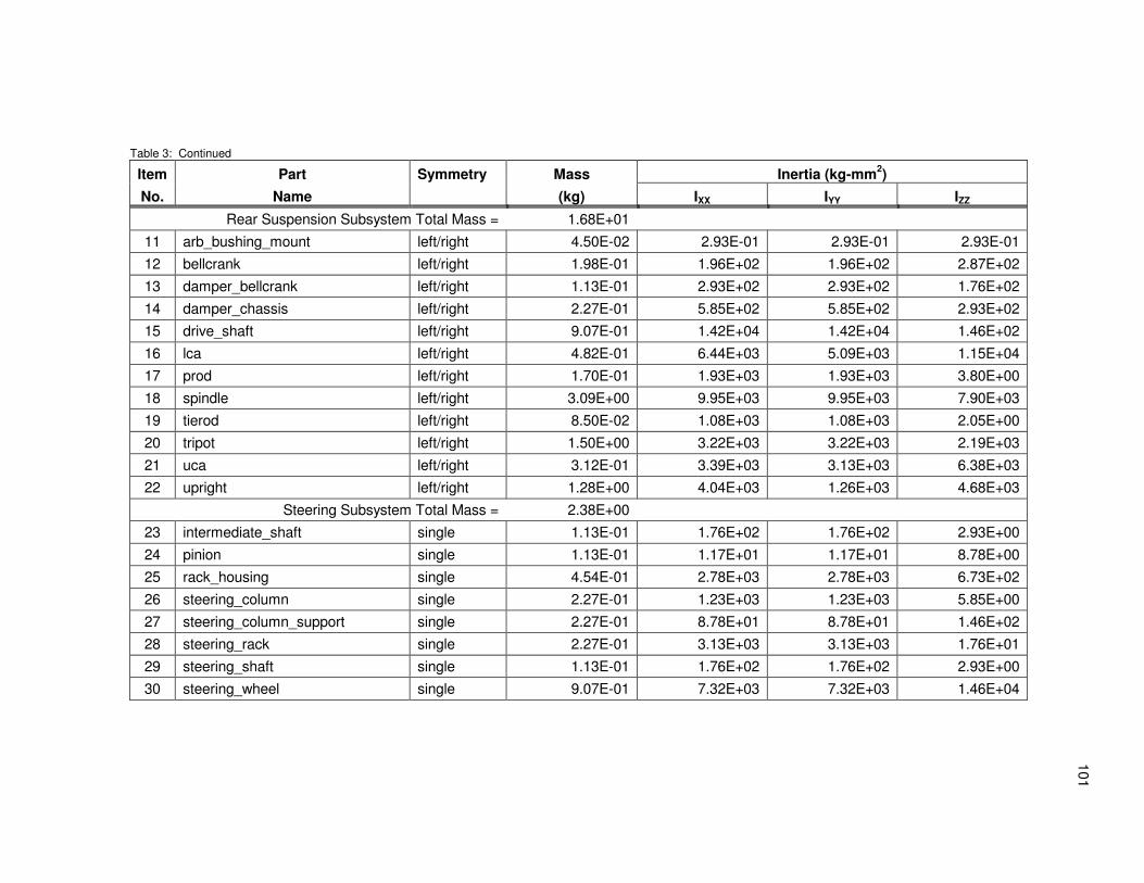
101

Table 3: Continued



Rear Suspension Subsystem Total Mass = 1.68E+01

11 arb_bushing_mount left/right 4.50E-02 2.93E-01 2.93E-01 2.93E-01

12 bellcrank left/right 1.98E-01 1.96E+02 1.96E+02 2.87E+02

13 damper_bellcrank left/right 1.13E-01 2.93E+02 2.93E+02 1.76E+02

14 damper_chassis left/right 2.27E-01 5.85E+02 5.85E+02 2.93E+02

15 drive_shaft left/right 9.07E-01 1.42E+04 1.42E+04 1.46E+02

16 lca left/right 4.82E-01 6.44E+03 5.09E+03 1.15E+04

17 prod left/right 1.70E-01 1.93E+03 1.93E+03 3.80E+00

18 spindle left/right 3.09E+00 9.95E+03 9.95E+03 7.90E+03

19 tierod left/right 8.50E-02 1.08E+03 1.08E+03 2.05E+00

20 tripot left/right 1.50E+00 3.22E+03 3.22E+03 2.19E+03

21 uca left/right 3.12E-01 3.39E+03 3.13E+03 6.38E+03

22 upright left/right 1.28E+00 4.04E+03 1.26E+03 4.68E+03

Steering Subsystem Total Mass = 2.38E+00

23 intermediate_shaft single 1.13E-01 1.76E+02 1.76E+02 2.93E+00

24 pinion single 1.13E-01 1.17E+01 1.17E+01 8.78E+00

25 rack_housing single 4.54E-01 2.78E+03 2.78E+03 6.73E+02

26 steering_column single 2.27E-01 1.23E+03 1.23E+03 5.85E+00

27 steering_column_support single 2.27E-01 8.78E+01 8.78E+01 1.46E+02

28 steering_rack single 2.27E-01 3.13E+03 3.13E+03 1.76E+01

29 steering_shaft single 1.13E-01 1.76E+02 1.76E+02 2.93E+00

30 steering_wheel single 9.07E-01 7.32E+03 7.32E+03 1.46E+04

102

Table 3: Continued



Powertrain Subsystem Total Mass = 4.20E+01

31 powertrain single 3.40E+01 1.46E+06 1.46E+06 1.46E+06

32 diff_output left/right 3.98E+00 2.05E+04 2.05E+04 1.17E+04

Front ARB Subsystem Total Mass = 1.80E-01

33 arb left/right 4.50E-02 1.81E+02 9.36E+01 9.36E+01

34 droplink left/right 4.50E-02 8.78E+01 8.78E+01 1.17E+00

Rear ARB Subsystem Total Mass = 1.80E-01

35 arb left/right 4.50E-02 9.66E+01 3.80E+01 1.34E+02

36 droplink left/right 4.50E-02 4.39E+02 4.39E+02 1.17E+00

Front Tires Subsystem Total Mass = 1.51E+01

37 wheel (including tire) left/right 7.57E+00 2.34E+05 2.34E+05 3.51E+05

Rear Tires Subsystem Total Mass = 1.51E+01

38 wheel (including tire) left/right 7.57E+00 2.34E+05 2.34E+05 3.51E+05

4 Wheel Brakes Subsystem Total Mass = 0.00E+00

no parts defined. 0.00E+00 0.00E+00 0.00E+00 0.00E+00

Total Mass (all parts except chassis) = 1.02E+02

103

Table 4: Hardpoint Locations

Item Hardpoint ACAR Model (mm)

No. I.D. Name Sym. z y z


1 A1 global single 0.00 0.00 0.00

2 A2 arblink_to_bellcrank left/right 867.73 -144.96 439.29

3 A3 arb_bushing_mount left/right 1000.00 -100.00 80.00

4 A4 bellcrank_pivot left/right 851.29 -188.08 402.09

5 A5 bellcrank_pivot_orient left/right 855.09 -255.09 478.21

6 A6 lca_front left/right 639.73 -172.12 85.69

7 A7 lca_outer left/right 852.61 -603.20 84.05

8 A8 lca_rear left/right 933.62 -171.10 84.69

9 A9 prod_outer left/right 846.36 -547.52 105.96

10 A10 prod_to_bellcrank left/right 894.97 -209.72 381.00

11 A11 shock_to_bellcrank left/right 867.73 -144.96 439.29

12 A12 shock_to_chassis left/right 661.58 -111.67 450.59

13 A13 tierod_inner left/right 989.92 -207.47 107.82

14 A14 tierod_outer left/right 981.69 -526.01 97.41

15 A15 uca_front left/right 662.90 -235.40 288.01

16 A16 uca_outer left/right 885.46 -601.94 314.11

17 A17 uca_rear left/right 1056.78 -234.31 284.50

18 A18 wheel_center left/right 858.46 -665.06 200.00

104

Table 4: Continued




19 B1 global single 0.00 0.00 0.00

20 B2 arblink_to_bellcrank left/right 2984.50 -139.70 342.90

21 B3 arb_bushing_mount left/right 2890.52 -114.30 127.00

22 B4 bellcrank_pivot left/right 2929.92 -189.88 293.66

23 B5 bellcrank_pivot_orient left/right 2877.32 -169.89 294.75

24 B6 drive_shaft_inr left/right 2760.00 -150.00 198.00

25 B7 lca_front left/right 2592.86 -208.62 77.36

26 B8 lca_outer left/right 2806.91 -586.38 90.32

27 B9 lca_rear left/right 2933.40 -211.47 73.28

28 B10 prod_outer left/right 2807.38 -537.01 105.74

29 B11 prod_to_bellcrank left/right 2890.99 -233.44 298.83

30 B12 shock_to_bellcrank left/right 2968.07 -150.48 326.51

31 B13 shock_to_chassis left/right 2972.25 -48.18 136.27

32 B14 tierod_inner left/right 2592.86 -208.62 77.36

33 B15 tierod_outer left/right 2692.51 -584.90 86.91

34 B16 uca_front left/right 2599.53 -251.44 272.10

35 B17 uca_outer left/right 2801.81 -585.27 320.03

36 B18 uca_rear left/right 2927.46 -248.68 269.95

37 B19 wheel_center left/right 2759.06 -582.41 198.04

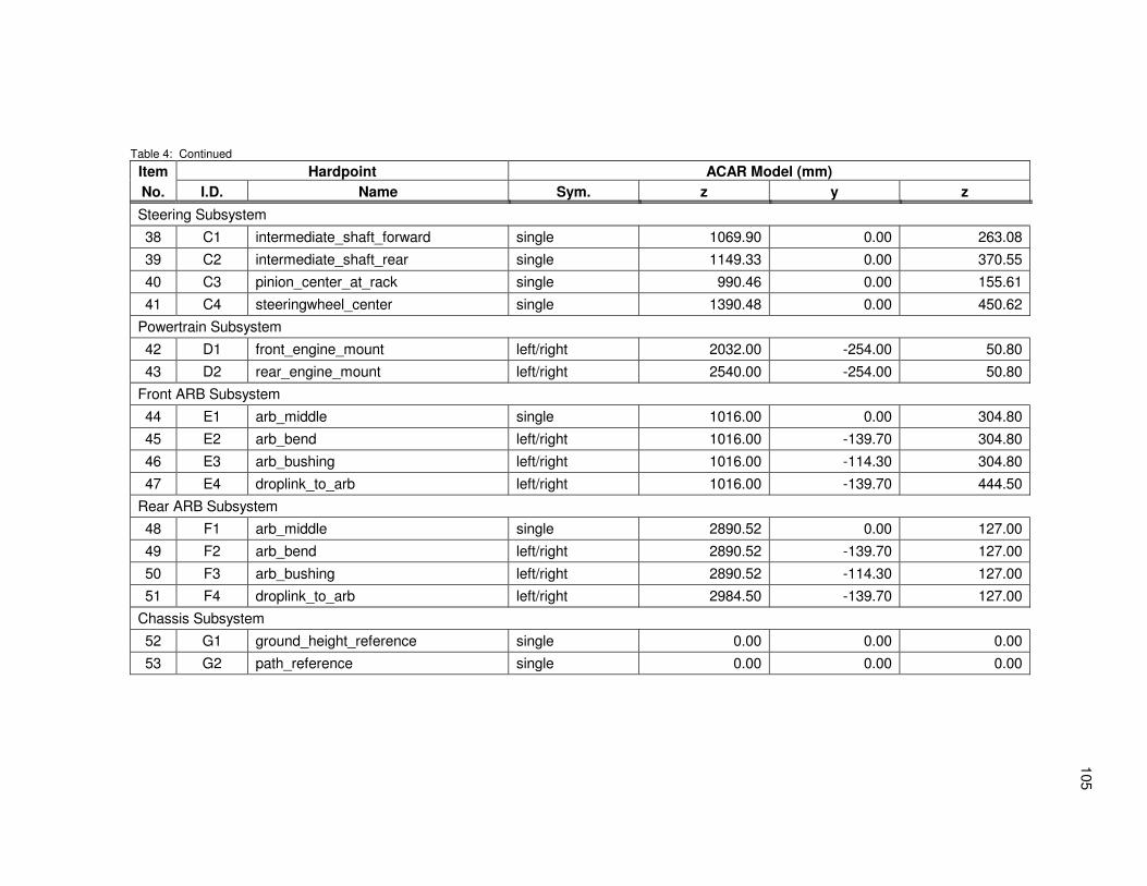
105

Table 4: Continued



Steering Subsystem

38 C1 intermediate_shaft_forward single 1069.90 0.00 263.08

39 C2 intermediate_shaft_rear single 1149.33 0.00 370.55

40 C3 pinion_center_at_rack single 990.46 0.00 155.61

41 C4 steeringwheel_center single 1390.48 0.00 450.62


42 D1 front_engine_mount left/right 2032.00 -254.00 50.80

43 D2 rear_engine_mount left/right 2540.00 -254.00 50.80

Front ARB Subsystem

44 E1 arb_middle single 1016.00 0.00 304.80

45 E2 arb_bend left/right 1016.00 -139.70 304.80

46 E3 arb_bushing left/right 1016.00 -114.30 304.80

47 E4 droplink_to_arb left/right 1016.00 -139.70 444.50

Rear ARB Subsystem

48 F1 arb_middle single 2890.52 0.00 127.00

49 F2 arb_bend left/right 2890.52 -139.70 127.00

50 F3 arb_bushing left/right 2890.52 -114.30 127.00

51 F4 droplink_to_arb left/right 2984.50 -139.70 127.00

Chassis Subsystem

52 G1 ground_height_reference single 0.00 0.00 0.00

53 G2 path_reference single 0.00 0.00 0.00

106

Table 5: Subsystem Parameters

Subsystem Parameter Name Symmetry Value Units

Front Susp. camber_angle left 0.0 deg

camber_angle right 0.0 deg

toe_angle left 0.0 deg

toe_angle right 0.0 deg

Rear Susp. camber_angle left 0.0 deg

camber_angle right 0.0 deg

drive_shaft_offset left 75.0 mm

drive_shaft_offset right 75.0 mm

toe_angle left 0.0 deg

toe_angle right 0.0 deg

Steering reduction_ratio1 single 0.0024 rev/mm

Powertrain bevel_gear single 1.0 gear ratio

clutch_damping2, 4

single 1.00E+005 No units

clutch_stiffness2, 4

single 1.00E+005 No units

clutch_torque_threshold2 single 1.00E+008 N-mm

drop_gear single 1.708 gear ratio

engine_idle_speed single 1500 rev/min

engine_rev_limit single 13500 rev/min

engine_rotational_inertia single 5853 N-mm2

final_drive single 4.909 gear ratio

gear_1 single 2.846 gear ratio






max_gears single 6 integer

max_throttle single 100 %

Front ARB torsional_spring_stiffness3 single 1.0 N-mm/deg

Rear ARB torsional_spring_stiffness3 single 1.0 N-mm/deg

Chassis aero_frontal_area4 single 1.275 No units

air_density4 single 1.225 No units

drag_coefficient4 single 0.5 No units

1ACAR defines a reduction ratio as a "gear assembly" and not as a parameter. The value is listed here for convenience.

2Arbitrary clutch parameters approximates a rigid connection between engine and transmission.

3Low stiffness assigned because 2002 racecar does not have anti-roll bars installed.

4Refer to ADAMS/Car Help Documentation > Templates > Rigid Chassis regarding unit convention.

107

Table 6: Bushing Stiffness and Damping Characteristics

Units Control Arm

Bushings Anti-Roll Bar

Bushings

FX Damping (force along x) N-s/mm 1.8E-01 1.8E-01

FY Damping (force along y) N-s/mm 1.8E-01 1.8E-01

FZ Damping (force along z) N-s/mm 1.8E-01 1.8E-01

TX Damping (torque about x) N-mm-s/deg 1.1E+01 1.1E+01

TY Damping (torque about y) N-mm-s/deg 1.1E+01 1.1E+01

TZ Damping (torque about z) N-mm-s/deg 1.1E+01 1.1E+01

FX Stiffness (force along x) N/mm 4.4E+04 4.4E+04

Total Travel (along x) mm 5.1E+00 5.1E+00

FY Stiffness (force along y) N/mm 4.4E+04 4.4E+04

Total Travel (along y) mm 5.1E+00 5.1E+00

FZ Stiffness (force along z) N/mm 4.4E+04 1.8E+01

Total Travel (along z) mm 5.1E+00 2.5E+01

TX Stiffness (torque about x) N-mm/deg 1.5E+00 1.1E+04

Total Travel (about x) deg 1.8E+02 1.2E+01

TY Stiffness (torque about y) N-mm/deg 1.5E+00 1.1E+04

Total Travel (about y) deg 1.8E+02 1.2E+01

TZ Stiffness (torque about z) N-mm/deg 1.5E+00 1.5E+00

Total Travel (about z) deg 1.8E+02 1.8E+02

108

Table 7: Pacejka ’94 Handling Force Model Tire Coefficients for Goodyear FSAE Tire

(20in outside diameter, 6.5in width, 13in diameter rim, 12psi inflation pressure)

Lateral Force Longitudinal Force Aligning Moment

A0 1.5000000E+00 B0 1.6226000E+00 C0 2.3500000E+00

A1 4.4255739E+01 B1 0.0000000E+00 C1 9.7149319E+00

A2 1.5523042E+03 B2 -1.5735423E+03 C2 -1.6034520E+00

A3 -3.5002492E+03 B3 -3.2753698E+01 C3 4.5126096E+00

A4 -1.5215217E+01 B4 -5.6439577E+02 C4 -2.6719007E+00

A5 6.6089451E-02 B5 3.5889021E-02 C5 1.2675784E-01

A6 -1.0564438E-02 B6 5.4078991E-03 C6 1.2924694E-01

A7 2.9197666E-01 B7 1.6524269E-01 C7 -3.0000000E-01

A8 -3.7541013E-02 B8 9.9999995E-01 C8 -2.1668433E+00

A9 8.5183467E-02 B9 8.9513884E-02 C9 -3.4857569E+00

A10 -3.1927707E-02 B10 2.9988183E-01 C10 3.0903661E-01

A11 -4.7678765E+01 B11 -9.1505449E+01 C11 1.5247976E-01

A12 -1.4027698E+02 B12 -1.1503518E+02 C12 3.2791519E-01

A13 8.8456962E-01 B13 4.8984496E-08 C13 1.8419775E-01

A14 -2.0369299E+01 C14 6.4124756E-02

A15 -3.8214868E-03 C15 4.7139574E-01

A16 -2.8742850E-02 C16 1.5927502E+00

A17 2.0000000E-01 C17 -1.6572575E+00

C18 -7.2889710E-02

C19 -1.8056243E-01

C20 -4.2424885E-01

Table 8: Pacejka ’94 Handling Force Model Parameters for Goodyear FSAE Tire

(20in outside diameter, 6.5in width, 13in diameter rim, 12psi inflation pressure)

Parameter Name Value Units

UNLOADED_RADIUS 2.6000000E-01 m

WIDTH 1.6510000E-01 m

ASPECT_RATIO 3.0000000E-01

VERTICAL_STIFFNESS 1.8018980E+05 N/m

VERTICAL_DAMPING 2.5000000E+02 N-s/m

LATERAL_STIFFNESS 9.0094900E+04 N/m

ROLLING_RESISTANCE 0.0000000E+00

109

Table 9: CG Locations – 2002 TAMU FSAE Racecar

Units Vehicle

Only Vehicle with

Driver Driver Only Ballast Only

Wheelbase mm 1900

Tire Radius (unloaded) mm 260

Mass kg 225.9 310.3 84.4 20.4

Mass on front axle kg 90.3 146.1 55.8 0

Mass on rear axle kg 135.6 164.2 28.6 20.4

Incline (front end lifted) deg 41.0 42.5

Mass on front axle kg 76.2 122.9

Mass on rear axle kg 149.7 187.3

XCG (behind front axle) mm 1141 1006 644 1900

ZCG (above ground) mm 396 415 464 520

Table 10: Chassis Part CG – Configuration 1 (75kg Driver, No Ballast)

Desired Total All Parts but

Chassis

M kg 3.012E+02 1.024E+02

XCG mm 1016.46 1230.91

ZCG mm 413.11 281.50

Driver Ballast Frame Chassis Part

M kg 7.530E+01 0.000E+00 1.235E+02 1.988E+02

XCG mm 643.55 1900.00 1066.00 905.98

ZCG mm 464.25 520.00 491.06 480.90

IXX kg-mm2 2.533E+04 0.000E+00 1.253E+07 1.256E+07

IYY kg-mm2 5.219E+06 0.000E+00 8.063E+07 8.585E+07

IZZ kg-mm2 5.197E+06 0.000E+00 7.859E+07 8.379E+07

IXY kg-mm2 4.690E-04 0.000E+00 9.536E+03 9.536E+03

IZX kg-mm2 3.309E+05 0.000E+00 1.596E+06 1.927E+06

IYZ kg-mm2 -4.690E-04 0.000E+00 -6.620E+03 -6.620E+03

110

Table 11: Chassis Part CG – Configuration 2 (88kg Driver, No Ballast)


Chassis

M kg 3.143E+02 1.024E+02

XCG mm 1000.85 1230.91

ZCG mm 415.25 281.50


M kg 8.845E+01 0.000E+00 1.235E+02 2.119E+02

XCG mm 643.55 1900.00 1066.00 889.69

ZCG mm 464.25 520.00 491.06 479.87

IXX kg-mm2 2.681E+04 0.000E+00 1.254E+07 1.256E+07

IYY kg-mm2 5.395E+06 0.000E+00 8.131E+07 8.671E+07

IZZ kg-mm2 5.373E+06 0.000E+00 7.927E+07 8.464E+07

IXY kg-mm2 5.510E-04 0.000E+00 9.536E+03 9.536E+03

IZX kg-mm2 3.422E+05 0.000E+00 1.639E+06 1.981E+06

IYZ kg-mm2 -5.510E-04 0.000E+00 -6.620E+03 -6.620E+03

Table 12: Chassis Part CG – Configuration 3 (75kg Driver, 20kg Ballast)


Chassis

M kg 3.216E+02 1.024E+02

XCG mm 1072.54 1230.91

ZCG mm 419.89 281.50


M kg 7.530E+01 2.041E+01 1.235E+02 2.192E+02

XCG mm 643.55 1900.00 1066.00 998.55

ZCG mm 464.25 520.00 491.06 484.54

IXX kg-mm2 3.546E+04 2.643E+04 1.253E+07 1.259E+07

IYY kg-mm2 9.532E+06 1.661E+07 7.803E+07 1.042E+08

IZZ kg-mm2 9.501E+06 1.659E+07 7.599E+07 1.021E+08

IXY kg-mm2 4.690E-04 0.000E+00 9.536E+03 9.536E+03

IZX kg-mm2 5.443E+05 6.521E+05 1.449E+06 2.646E+06

IYZ kg-mm2 -4.690E-04 0.000E+00 -6.620E+03 -6.620E+03

111

Table 13: Chassis Part CG – Configuration 4 (88kg Driver, 20kg Ballast)


Chassis

M kg 3.348E+02 1.024E+02

XCG mm 1055.68 1230.91

ZCG mm 421.63 281.50


M kg 8.845E+01 2.041E+01 1.235E+02 2.323E+02

XCG mm 643.55 1900.00 1066.00 978.45

ZCG mm 464.25 520.00 491.06 483.40

IXX kg-mm2 3.765E+04 2.812E+04 1.253E+07 1.259E+07

IYY kg-mm2 9.967E+06 1.736E+07 7.841E+07 1.057E+08

IZZ kg-mm2 9.934E+06 1.734E+07 7.638E+07 1.036E+08

IXY kg-mm2 5.510E-04 0.000E+00 9.536E+03 9.536E+03

IZX kg-mm2 5.692E+05 6.883E+05 1.478E+06 2.736E+06

IYZ kg-mm2 -5.510E-04 0.000E+00 -6.620E+03 -6.620E+03

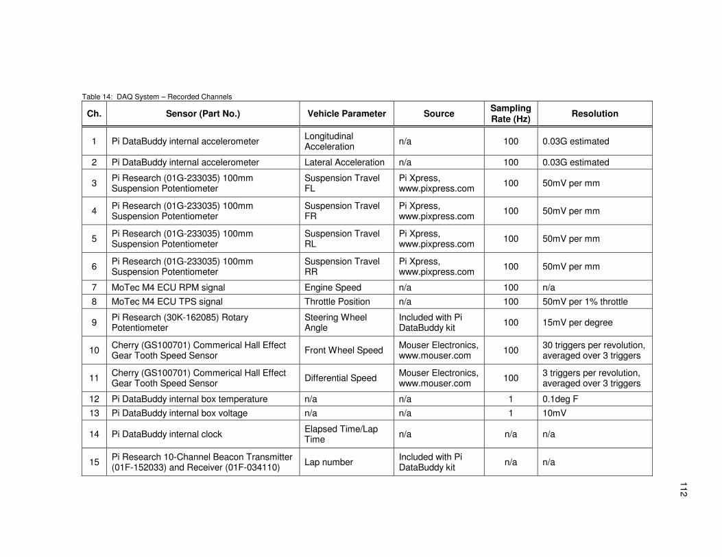
112

Table 14: DAQ System – Recorded Channels

Ch. Sensor (Part No.) Vehicle Parameter Source Sampling Rate (Hz)

Resolution

1 Pi DataBuddy internal accelerometer Longitudinal Acceleration

n/a 100 0.03G estimated

2 Pi DataBuddy internal accelerometer Lateral Acceleration n/a 100 0.03G estimated

3 Pi Research (01G-233035) 100mm Suspension Potentiometer

Suspension Travel FL

Pi Xpress, www.pixpress.com

100 50mV per mm


Suspension Travel FR


100 50mV per mm


Suspension Travel RL


100 50mV per mm


Suspension Travel RR


100 50mV per mm

7 MoTec M4 ECU RPM signal Engine Speed n/a 100 n/a

8 MoTec M4 ECU TPS signal Throttle Position n/a 100 50mV per 1% throttle

9 Pi Research (30K-162085) Rotary Potentiometer

Steering Wheel Angle

Included with Pi DataBuddy kit

100 15mV per degree

10 Cherry (GS100701) Commerical Hall Effect Gear Tooth Speed Sensor

Front Wheel Speed Mouser Electronics, www.mouser.com

100 30 triggers per revolution, averaged over 3 triggers

11 Cherry (GS100701) Commerical Hall Effect Gear Tooth Speed Sensor

Differential Speed Mouser Electronics, www.mouser.com

100 3 triggers per revolution, averaged over 3 triggers

12 Pi DataBuddy internal box temperature n/a n/a 1 0.1deg F

13 Pi DataBuddy internal box voltage n/a n/a 1 10mV

14 Pi DataBuddy internal clock Elapsed Time/Lap Time

n/a n/a n/a

15 Pi Research 10-Channel Beacon Transmitter (01F-152033) and Receiver (01F-034110)

Lap number Included with Pi DataBuddy kit

n/a n/a

113

VITA

Name: Russell Lee Mueller

Address: Bell Helicopter Textron, P.O. Box 482, Mail Drop 38-1, Machining Center of

Excellence (Plant 5), Fort Worth, TX 76101

Education: B.S., Mechanical Engineering, Texas A&M University, 2000

M.S., Mechanical Engineering, Texas A&M University, 2005

FULL VEHICLE DYNAMICS MODEL OF A FORMULA SAE...

Documents

Transcript of FULL VEHICLE DYNAMICS MODEL OF A FORMULA SAE...