Full scale VIV response measurements of a drill pipe in Gulf of Mexico loop currents (OMAE2008-57610)Beynet, Shilling, Campbell, Tellier, HowellsEstoril

Portugal -

June 2008

The Test

•

September 2004

•

Test of opportunity

•

Waiting on weather to run conductor (~2 knot surface currents)

•

VIV monitoring system already on the rig

•

6-5/8 inch drill pipe was instrumented and deployed to 1,000ft water depth

•

On-board acoustic doppler

current profiler (ADCP) measured current

6040 ft

Keel 6000 ft

Drill floor 6133 ft

1080 ft

Vessel mounted motion logger

5 motion loggers

6040 ft

Keel 6000 ft

Drill floor 6133 ft

1080 ft

Vessel mounted motion logger

5 motion loggers

Did it VIV?

Agenda

•

Background

−

Test set up

−

Monitoring system

−

Test timeline

•

Observed response

−

VIV occurrence and effect of changing current

−

Single mode, multi-mode or time sharing?

−

Higher harmonics

−

Standing or travelling wave

•

Conclusions

Test set-up

•

1080 ft length

•

6-5/8 inch OD

•

0.492 inch wall thickness

•

32.2 lb/ft (47.9 kg/m) in air

•

80ksi strength, carbon steel

•

Drill pipe was free flooding –

water filled up to mean water line

6040 ft

Keel 6000 ft

Drill floor 6133 ft

1080 ft

Vessel mounted motion logger

5 motion loggers

6040 ft

Keel 6000 ft

Drill floor 6133 ft

1080 ft

Vessel mounted motion logger

5 motion loggers

VIV monitoring system

•

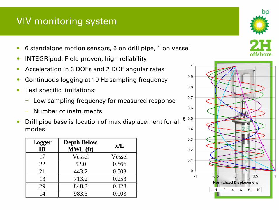
6 standalone motion sensors, 5 on drill pipe, 1 on vessel

•

INTEGRIpod: Field proven, high reliability

•

Acceleration in 3 DOFs

and 2 DOF angular rates

•

Continuous logging at 10 Hz sampling frequency

•

Test specific limitations:

−

Low sampling frequency for measured response

−

Number of instruments

•

Drill pipe base is location of max displacement for all modes

Logger ID

Depth Below MWL (ft) x/L

17 Vessel Vessel 22 52.0 0.866 21 443.2 0.503 13 713.2 0.253 29 848.3 0.128 14 983.3 0.003

0

0.1

0.2

0.3

0.4

0.5

0.6

0.7

0.8

0.9

1

-1 -0.5 0 0.5 1

Normalized Displacementx/

L1 2 4 6 8 10

Current measurement

•

38 KHz Acoustic Doppler Current Profiler (ADCP)

•

Designed for measurement of ocean currents

•

Provides 10 minute average

speed and direction

•

Measures 95ft to 3,600ft below surface every 100ft

•

Max measured current = 1.8 knot

•

Strouhal

(0.20) frequency = 1.1 Hz

•

50ft missing between drill ship keel and first data point

•

Vessel mounted system measures effective current on drill pipe whilst drifting (which we want)

0.0 100.0 200.0 300.0

Current Direction (degrees)

0

100

200

300

400

500

600

700

800

900

1000

0.0 0.5 1.0 1.5 2.0

Current Speed (knots)

Dep

th B

elow

MW

L (f

t)

#2 #5 #13 #19

KEEL

Test timeline

•

2 hour test with 16:03 (4:03pm) start time

•

Vessel drift relative to the current was varied

•

Objective: Determine effect of maintaining vertical pipe

Time Vessel Drift Information 16:00 Varying vessel drift, speed unknown

17:08 Vessel drift at 1.8 knots in current direction

17:17 Reduce drift speed to 0 knot 17:28 Vessel at 0 knot

17:38 Increase vessel drift to 1 knot in current direction

Vessel stationary

Current ~1.8 knots

Vessel stationary

Current ~1.8 knots

Vessel drift – vertical pipe

Current

Vessel drift – vertical pipe

Current

Vessel drift = surface current

Current ~1.8 knots

Vessel drift = surface current

Current ~1.8 knots

Drill pipe response at base –

0 to 30 minutes

•

X and Y waterfall plots side by side

Varying vessel drift with current –

Objective: maintain vertical pipe

Approx max cross flow frequency (St=0.20)

Water fall Plots X and Y (Lateral) Accelerations

0

100

200

300

400

500

600

700

800

900

1000

-1.5 -1.0 -0.5 0.0 0.5 1.0 1.5

Current Speed (knots)

Dep

th B

elo

w M

WL

(ft)

KEEL

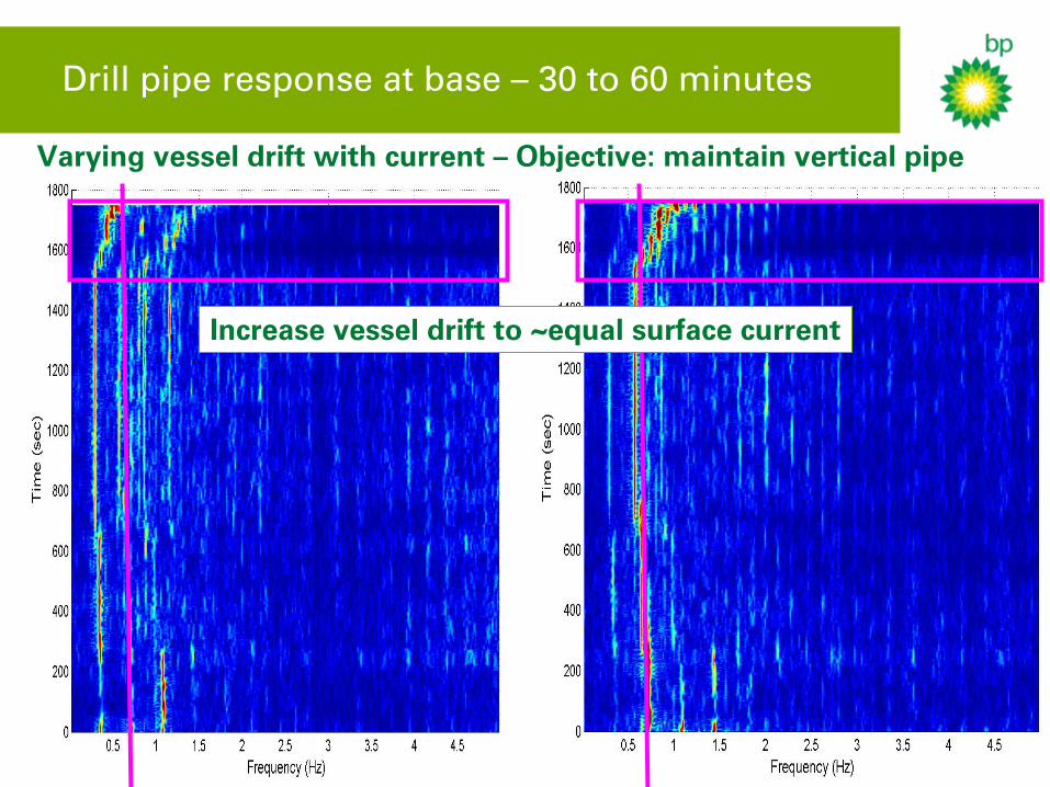
Drill pipe response at base –

30 to 60 minutes

•

X and Y waterfall plots side by side

Varying vessel drift with current –

Objective: maintain vertical pipe

Increase vessel drift to ~equal surface current

Drill pipe response at base –

60 to 90 minutes

•

X and Y waterfall plots side by side

Multi-mode cross flow VIV6th

Higher harmonic

0

100

200

300

400

500

600

700

800

900

1000

-2.0 -1.5 -1.0 -0.5 0.0 0.5 1.0

Current Speed (knots)

Dep

th B

elo

w M

WL

(ft)

KEEL

Reduce drift to zero knots, return to loop current profile

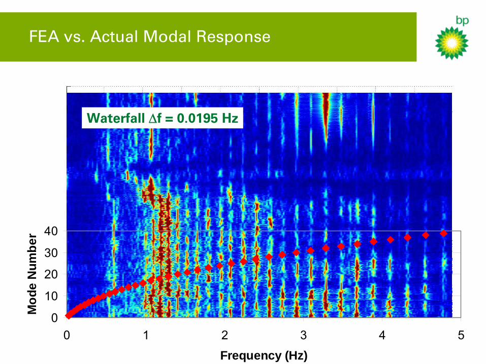
FEA vs. Actual Modal Response

0

10

20

30

40

0 1 2 3 4 5Frequency (Hz)

Mod

e N

umbe

r

Waterfall Δf

= 0.0195 Hz

Drill pipe response at base –

90 to 120 minutes

•

X and Y waterfall plots side by side

Single mode cross flow VIVStrong 6th

harmonic

Return to varying vessel drift with currentObjective: maintain vertical pipe

0

100

200

300

400

500

600

700

800

900

1000

-0.5 0.0 0.5 1.0 1.5 2.0

Current Speed (knots)

Dep

th B

elo

w M

WL

(ft)

KEEL

Severity of higher harmonics –

90 to 95 minutes

•

Higher harmonic fatigue damage is negligible compared to cross flow

•

Conflicts with test findings –

fatigue from higher harmonics > factor of 10

•

Fatigue damage calculation assumes standing wave

0

0.2

0.4

0.6

0.8

1

1.2

0.55 1.1 1.65 3.3

Frequency (Hz)

Nor

mal

ized

to

Max

imu

m

Displacement Fatigue Damage

Cross flow

In-line3rd

Harmonic6th

Harmonic

Standing or travelling wave?

•

Standing wave typically assumed in design

•

High fatigue damage along the entire length if travelling wave

•

If 100% standing wave there will be locations of zero measured motion and fatigue along length

•

If 100% travelling wave measured motion envelopes and fatigue along length will be similarStanding Wave Travelling Wave

Spectral response along pipe -

90 to 95 minutes

CrossflowVIV

3rd

Harmonic6th

Harmonic?

Theoretical standing wave vs. measurements

0

0.2

0.4

0.6

0.8

1

1.2

1.4

1.6

0 0.2 0.4 0.6 0.8 1

x/L

Acc

(m

/s^

2)

Measured Theoretical at Measurement Locations Theoretical

•

Measured Accelerations at 0.552Hz with Mode 10 Superposed

•

Measured response fits standing wave

Are the higher harmonics standing wave?

3.3 Hz response is theoretically mode 32

Varying amplitude:standing wave?

Conclusions

•

Strong BP on-shore and offshore teamwork allowed test of opportunity

•

Valuable data set that complements and extends existing tests

•

Observed single mode, multi-mode and time sharing VIV

•

Time sharing typically coincides with changes in vessel drift speed

•

Higher harmonics up to 6 times cross flow VIV observed

•

Cross flow VIV fatigue damage dominates

•

Contribution of dynamic positioning prop wash excitation is uncertain

•

VIV response is standing wave, up to mode 14, possibly mode 32

•

Greatest VIV risk: short term temporary operations in high currents

•

Drifting to maintain verticality recommended to minimize VIV

Questions?

Spatial aliasing example

Spacial Aliasing

-1.5

-1

-0.5

0

0.5

1

1.5

0 0.1 0.2 0.3 0.4 0.5 0.6 0.7 0.8 0.9 1

Length (units)

Am

plitu

de (u

nits

)

Number of loggers 5 Number of nodes/antinodes 3

Mode Shape No.of

Loggers

Logger Start Locn

Spacial Aliasing

-1.5

-1

-0.5

0

0.5

1

1.5

0 0.1 0.2 0.3 0.4 0.5 0.6 0.7 0.8 0.9 1

Length (units)

Am

plitu

de (u

nits

)

Number of loggers 5 Number of nodes/antinodes 7

Mode Shape No.of

Loggers

Logger Start Locn

FEA vs. Actual Modal Response

0

10

20

30

40

0 1 2 3 4 5Frequency (Hz)

Mod

e N

umbe

r

Waterfall Δf

= 0.0195 Hz