
Chapter8.Lagrangiansubmanifoldsinsemi-positivesymplecticmani-fukaya/Chapter81110.pdf ·...
149
Chapter 8. Lagrangian submanifolds in semi-positive symplectic mani- folds. 1 §34. Statement of the results in Chapter 8. So far we have been studying Floer cohomology with rational coefficients. If we put some additional assumptions on our symplectic manifold, Floer cohomology can be defined over Z coefficients or Z 2 coefficients. In this chapter, we discuss this point and its applications. We remark that in Chapters 3-5, we developed the homological algebra also with the coefficient ring of Z or Z 2 . So the necessary algebraic part of the story has already been generalized. We first recall the following : Definition 34.1. ([McD91]) A 2n-dimensional symplectic manifold (M,ω) is called semi-positive if ω(β ) ≤ 0 for any β ∈ π 2 (M ) with 3 − n ≤ c 1 (M )[β ] < 0. Remark 34.2. (1) Note that if n ≤ 3, the semi-positivity automatically holds. (2) An n-dimensional Lagrangian submanifold L ⊂ (M,ω) is called semi-positive if ω(β ) ≤ 0 for any β ∈ π 2 (M,L) with 3 − n ≤ μ L (β ) < 0. If L ⊂ (M,ω) is semi- positive, then (M,ω) itself must be semi-positive. We do not assume semi-positivity of L but only assume semi-positivity of M . For R = Q, Z or Z 2 = Z/2Z, we put Λ R 0,nov = n X a i T ∏ i e n i Ø Ø Ø ∏ i ∈ R ≥0 ,n i ∈ Z,a i ∈ R, lim i→1 ∏ i = 1 o . We define Λ R nov ,Λ +R 0,nov in the same way. (In Chapters 1,3,4,5,6,7, it is written as Λ 0,nov (R) in place of Λ R 0,nov .) Condition 34.3. We assume that there exists a compatible almost complex struc- ture J on M such that every J -holomorphic sphere v : S 2 → M with c 1 (M )[v]=0 is constant. For example CP n , C n , T 2n or any monotone symplectic manifolds satisfy Con- dition 34.3. The first main result of this chapter is : Theorem 34.4. Let L ⊂ (M,ω) be a relatively spin Lagrangian submanifold. We assume (M,ω) is semi-positive and satisfies Condition 34.3. Then we have the following : (1) The filtered A 1 algebra (C (L), m ∗ ) in Theorem 10.11 is defined over Λ Z 0,nov . We write it as (C (L;Λ Z 0,nov ), m ∗ ) . 1 Version: NOv. 10, 2007 1
Transcript of Chapter8.Lagrangiansubmanifoldsinsemi-positivesymplecticmani-fukaya/Chapter81110.pdf ·...

Chapter 8. Lagrangian submanifolds in semi-positive symplectic mani-folds.1
§34. Statement of the results in Chapter 8.
So far we have been studying Floer cohomology with rational coefficients. If weput some additional assumptions on our symplectic manifold, Floer cohomology canbe defined over Z coefficients or Z2 coefficients. In this chapter, we discuss this pointand its applications. We remark that in Chapters 3-5, we developed the homologicalalgebra also with the coefficient ring of Z or Z2. So the necessary algebraic part ofthe story has already been generalized. We first recall the following :
Definition 34.1. ([McD91]) A 2n-dimensional symplectic manifold (M,ω) is calledsemi-positive if ω(β) ≤ 0 for any β ∈ π2(M) with 3− n ≤ c1(M)[β] < 0.
Remark 34.2.(1) Note that if n ≤ 3, the semi-positivity automatically holds.(2) An n-dimensional Lagrangian submanifold L ⊂ (M,ω) is called semi-positiveif ω(β) ≤ 0 for any β ∈ π2(M,L) with 3 − n ≤ µL(β) < 0. If L ⊂ (M,ω) is semi-positive, then (M,ω) itself must be semi-positive. We do not assume semi-positivityof L but only assume semi-positivity of M .
For R = Q, Z or Z2 = Z/2Z, we put
ΛR0,nov =
nXaiT
∏ieni
ØØØ ∏i ∈ R≥0, ni ∈ Z, ai ∈ R, limi→1
∏i = 1o
.
We define ΛRnov, Λ+R
0,nov in the same way. (In Chapters 1,3,4,5,6,7, it is written asΛ0,nov(R) in place of ΛR
0,nov.)
Condition 34.3. We assume that there exists a compatible almost complex struc-ture J on M such that every J-holomorphic sphere v : S2 → M with c1(M)[v] = 0is constant.
For example CPn, Cn, T 2n or any monotone symplectic manifolds satisfy Con-dition 34.3. The first main result of this chapter is :
Theorem 34.4. Let L ⊂ (M,ω) be a relatively spin Lagrangian submanifold. Weassume (M,ω) is semi-positive and satisfies Condition 34.3. Then we have thefollowing :(1) The filtered A1 algebra (C(L),m∗) in Theorem 10.11 is defined over ΛZ
0,nov.We write it as (C(L;ΛZ
0,nov),m∗).
1Version: NOv. 10, 2007
1

2 FUKAYA, OH, OHTA, ONO
(2) If we take the Z-reduction, see (7.13), the cohomology ring of (C(L; Z),m∗) isisomorphic to the cohomology ring H(L; Z) of L.(3) (C(L;ΛZ
0,nov),m∗) has a homotopy unit.(4) Theorem 14.1 is generalized to this case. Namely if √ : M → M is a sym-plectic diffeomorphism and L0 = √(L) then it induces a homotopy-unital homotopyequivalence √∗ : (C(L;ΛZ
0,nov),m∗) → (C(L0;ΛZ0,nov),m∗). (See §15.3). Theorem
14.2 is also generalized to this case.(5) If (L(1), L(0)) is a relatively spin pair of clean intersection, then the filtered A1bimodule C(L(1), L(0);Λ0,nov) is defined over ΛZ
0,nov. Namely we have C(L(1), L(0);ΛZ0,nov)
which is a homotopy-unital filtered A1 bimodule over C(L(1);ΛZ0,nov) - C(L(0);ΛZ
0,nov).(6) Theorems 22.1 and 22.4 (invariance of the filtered A1 bimodule under the ac-tion of symplectic diffeomorphisms and under the Hamiltonian isotopy) over the ringΛZ
0,nov hold. Consequently, Theorems 14.3 and 14.4 (invariance of Floer cohomology)hold.(7) Theorems 11.18 and 11.43 (sequence of obstruction classes) over ΛZ
0,nov hold.(8) For any field R, (24.6.1) and (24.6.2) in Theorem 24.5 (the spectral sequencecalculating Floer cohomology) remain to be the case after replacing the coefficientring ΛZ
0,nov by ΛR0,nov. Theorem 24.10 also holds.
(9) If L is rational and rationally unobstructed with Z-coefficients, then the spec-tral sequence converges with the coefficient ring ΛZ
0,nov. More specifically, the con-struction in §25, especially (25.7), remains to hold.
Remark 34.5. As we mentioned in the introduction, it is very likely that Condition34.3 can be removed. Since the argument for it is more involved and this conditionis satisfied in the situations when we apply it in this book, we assume it in thisbook, and postpone the discussion to remove it to a paper which we are planing towrite.
Note that for the case R = Z, we do not have the canonical models (see §23)of filtered A1 algebra and filtered A1 bimodule. Thus we can not state the Z-coefficients versions of Theorems A and F in terms of cohomology as in Chapter 1,but can state the corresponding results by using the filtered A1 algebra C(L;ΛZ
0,nov)in Theorem 34.4 (1) and the filtered A1 bimodule C(L(1), L(0);ΛZ
0,nov) in Theorem34.4 (5). Indeed, the following theorems are just restatement of some parts ofTheorem 34.4, which are regarded as the semi-positive versions of Theorems A andF mentioned in Chapter 1.
Theorem As. Let L ⊂ (M,ω) be a relatively spin Lagrangian submanifold. Weassume (M,ω) is semi-positive and satisfies Condition 34.3. Then we can constructthe filtered A1 algebra (C(L;ΛZ
0,nov),m∗) over ΛZ0,nov as in Theorem 34.4 (1).
If √ : (M,L) → (M 0, L0) is a symplectic diffeomorphism, then we can associateto it an isomorphism √∗ := (√−1)∗ : C(L;ΛZ
0,nov) → C(L0;ΛZ0,nov) of filtered A1
algebras whose homotopy class depends only of isotopy class of symplectic diffeo-morphism √ : (M,L) → (M 0, L0).

CHAPTER 8. LAGRANGIAN IN SEMI-POSITIVE SYMPLECTIC MANIFOLD 3
The Poincare dual PD([L]) ∈ C0(L;ΛZ0,nov) of the fundamental cycle [L] is the
homotopy unit of our filtered A1 algebra. The homomorphism √∗ is homotopy-unital.
Theorem Fs. Let (L(1), L(0)) be a relatively spin pair of Lagrangian submanifoldsof (M,ω). Assume that L(0) and L(1) intersect cleanly. We assume (M,ω) is semi-positive and satisfies Condition 34.3. Then we can construct the filtered A1 bimod-ule C(L(1), L(0);ΛZ
0,nov) as in Theorem 34.4(5). Namely we have C(L(1), L(0);ΛZ0,nov)
which is a homotopy-unital filtered A1 bimodule over C(L(1);ΛZ0,nov) - C(L(0);ΛZ
0,nov).
Remark 34.6. There are several results in the previous chapters whose validity forthe Z coefficient in the of semi-positive case is still not clear to us. We make somecomments on them here. Among them, (1), (2) and (4) also apply to Theorem 34.7below :
(1) Both the statement and the proof of Theorem 33.1 in §33 are based on the deRham theory and so are valid for the coefficient ring R. However it is clear fromthe proof given below that the induced A1 algebra (C(L;ΛZ
0,nov),m∗) obtainedby reducing the coefficient ring to Z is homotopy equivalent to the A1 algebraconstructed in Theorem 9.8. In this sense, Theorem 33.1 (comparison of our filteredA1 algebra to it classical part) is also generalized over Z.(2) In a discussion of §13, we used the fact that our Novikov ring contains Q.Therefore constructions of the operators q, p do not apply for the ΛZ
0,nov coefficient.Because of this, the proof of Theorem 13.41 is not generalized over the ΛZ
0,nov
coefficients, and hence not Theorem 13.41 itself. Similar remarks apply to (24.6.3)of Theorem 24.5.(3) When L is irrational, it is not clear to us whether the convergence result ofthe spectral sequence in Theorem 24.5 holds over ΛZ
0,nov. (See the paragraph rightafter Theorem 24.10.)(4) As we mentioned above, we do not have the canonical model over Z. However,the construction given in §23 yields the following, (see also §27.1.) : Let L be a rela-tively spin Lagrangian submanifold of a semi-positive symplectic manifold satisfyingCondition 34.3. Then for any subcomplex C of C(L; Z) which is a direct summandas a Z-module and induces an isomorphism in cohomology with Z-coefficients, wehave a structure of filtered A1 algebra on C ⊗ΛZ
0,nov. The filtered A1 structure isindependent of choices up to homotopy equivalence. Thus if the cohomology groupH(L; Z) is a torsion free Z-module, then there is a structure of filtered A1 algebraon H(L; Z) ⊗ ΛZ
0,nov. Moreover, for any CW or simplicial decomposition of L wecan define a structure of filtered A1 algebra on the cochain complex over ΛZ
0,nov
which is associated to the cellular or simplicial decomposition.
In the semi-positive case, we can also work over Z2 which enables us to generalizevarious results of Chapter 6 for L that is neither orientable nor relatively spin.Because the Maslov index can be odd for unorientable L, we need to enlarge our

4 FUKAYA, OH, OHTA, ONO
Novikov ring to ΛZ20,nov[e1/2] so that it includes the square root e1/2. Recall that
deg e = 2 in our definition.
Theorem 34.7. Let L ⊂ (M,ω) be a Lagrangian submanifold, not necessarilyrelatively spin. We assume (M,ω) is semi-positive and satisfies Condition 34.3.Then, we can still define a unital filtered A1 algebra (C(L;ΛZ2
0,nov[e1/2]),m∗) as inTheorem 10.11. If L(1), L(0) are semi-positive Lagrangian submanifolds, then theA1 bimodule C(L(1), L(0);ΛZ2
0,nov[e1/2]) is defined.Theorems 14.1, 14.2, 14.3, 14.4, 22.1, 22.11 and Theorem 24.5 (24.6.1), (24.6.2),
and Theorem 24.10 are generalized to this case.
Theorems Bs, Cs, Ds, Es, Gs in the introduction directly follow from Theorems34.4 and 34.7.
For the case R = Z2, we have the canonical model, since Z2 is a field. SoTheorems A and F can be generalized directly to the situation of Theorem 34.5over ΛZ2
0,nov[e1/2].
Using Theorem 34.7 we have the following result which is similar to Corollary24.20. This is nothing but Theorem L (1) in Chapter 1.
Corollary 34.8. Let L ⊂ M be a Lagrangian submanifold. We assume (M,ω)satisfies Condition 34.3, H2(L; Z2) = 0, and there is a Hamiltonian diffeomorphismφ such that
L ∩ φ(L) = ∅.
Then the Maslov index homomorphism µL : π2(M,L) → Z is not trivial.
Proof. We will prove this by contradiction. Suppose to the contrary that µL istrivial for L. This in particular implies that L is semi-positive by definition. Hence(M,ω) is semi-positive. Since µL is trivial, all the obstruction classes for the Floercohomology over Z2 coefficients lie in H2(L; Z2) = 0 because n − (n − 2 + µL) =2. Since we assume H2(L; Z2) = 0, all obstructions automatically vanish and sowe derive M(L; Z2) 6= ∅. Now let b ∈ M(L; Z2) and consider the correspondingFloer cohomology HF ((L, b), (L, b)) ∼= HF ((L, b), (φ(L),φ∗(b)) is well defined. Theassumption L ∩ φ(L) = ∅ then implies HF ((L, b), (L, b)) = 0. On the other hand,Theorem 24.12 is generalized to the Z2 coefficient for the semi-positive case andimplies that HF ((L, b), (L, b)) cannot be zero which gives rise to a contradiction. §
Proof of Theorem Ks. Note that Cn is noncompact but bounded at infinity. There-fore all the theorems in this book apply to compact Lagrangian submanifolds ofCn. For given compact Lagrangian submanifold L, we can easily find a Hamilton-ian diffeomorphism φ : Cn → Cn of compact support such that L ∩ φ(L) = ∅. NowCorollary 34.8 finishes the proof. §
We now point out some main ideas in the proofs of Theorems 34.4 and 34.7,which deal with the case of the Z coefficients. Note that the only reason for the

CHAPTER 8. LAGRANGIAN IN SEMI-POSITIVE SYMPLECTIC MANIFOLD 5
usage of rational cycles, instead of integral ones, in the stable map compactificationcomes from the fact that the (finite) automorphism groups of stable maps we usecould be non-trivial. A simple examination of the constructions in [FuOn99II] or inChapter 7 of this book, however, shows that all the construction would work withthe Z or Z2 coefficients, without assuming any other condition, as long as all thestable maps involved in the construction have trivial automorphism groups.
In this respect, the following observation is important, although its proof imme-diately comes from the structure of PSL(2; R).
Lemma 34.9. The automorphism group of a semi-stable bordered Riemann surface(Σ,~z) ∈Mmain
k+1 of genus 0 is torsion free if k ≥ 0 and if it has no sphere components.In particular, if a stable map ((Σ,~z), w) ∈ Mmain
k+1 (J ;β) with k ≥ 0 has no spherebubbles, then the automorphism group of ((Σ,~z), w) is trivial.
Here we specify J , the almost complex structure, in the notation Mmaink+1 (J ;β)
above, since the results of Chapter 8 (for example Theorem 34.11 below) may nothold for arbitrary J but is correct only after choosing J appropriately. (For theresults of Chapter 3 ∼ 7, we may take any J , since the perturbation we use is anabstract perturbation.) An immediate corollary is the following :
Corollary 34.10. Let k ≥ 0. If an element ((Σ,~z), w) ∈ Mmaink+1 (J ;β) does not
have sphere components, then ((Σ,~z), w) ∈Mmaink+1 (J ;β) have trivial automorphism
group. In particular, if (M,ω, J) does not allow any pseudo-holomorphic spherethen its automorphism group is trivial.
Let us now assume that (M,ω) is semi-positive and satisfies Condition 34.3.Hereafter we will use a compatible almost complex structure for which there existsno pseudo-holomorphic sphere v : S2 → M with c1(M)[v] ≤ 0 other than constantmaps.
Now we consider the moduli space
Mmaink+1 (β;P1, · · · , Pk) := Mmain
k+1 (J ;β)×(ev1,··· ,evk) (P1 × · · ·× Pk).
We have a natural decomposition such that
Mmaink+1 (β;P1, · · · , Pk)
= Mmaink+1 (β;P1, · · · , Pk)free ∪Mmain
k+1 (β;P1, · · · , Pk)fix.
Here Mmaink+1 (β;P1, · · · , Pk)free (resp. Mmain
k+1 (β;P1, · · · , Pk)fix) is the set of elementswith trivial (resp. nontrivial) automorphism groups. The following theorem is themain step of the proofs of Theorems 34.4 and 34.7.
Theorem 34.11. We assume (M,ω) is semi-positive and satisfies Condition 34.3.Let L ⊂ (M,ω) be a Lagrangian submanifold and let P1, · · · , Pk be given singular

6 FUKAYA, OH, OHTA, ONO
simplices and β ∈ Π(M ;L). Consider the moduli space Mmaink+1 (β;P1, · · · , Pk) and
its decomposition given above. Then there exists a family of single valued piece-wise smooth sections s≤ of the obstruction bundle in a Kuranishi neighborhood ofMmain
k+1 (β;P1, · · · , Pk) and a decomposition
(34.12)Mmain
k+1 (β;P1, · · · , Pk)s≤
= Mmaink+1 (β;P1, · · · , Pk)s≤
free ∪Mmaink+1 (β;P1, · · · , Pk)s≤
fix
of the perturbed moduli space such that :
(34.13.1) Mmaink+1 (β;P1, · · · , Pk)s≤
free is a PL manifold.(34.13.2) Mmain
k+1 (β;P1, · · · , Pk)s≤
has a triangulation compatible with the smoothstructure on Mmain
k+1 (β;P1, · · · , Pk)s≤
free.(34.13.3) π(Mmain
k+1 (β;P1, · · · , Pk)s≤
fix) is contained in a sub-complex of dimension
dimMmaink+1 (β;P1, · · · , Pk)s≤
free − 2.
(34.13.4) lim≤→0 s≤ = s, where s is the original Kuranishi map overMmain
k+1 (β;P1, · · · , Pk) which is constructed in Chapter 7.
Once Theorem 34.11 (and the analogous statements for other moduli spaces usedin previous chapters) is proven, the rest of the proofs of Theorems 34.4 and 34.7 arethe straightforward analogs of the arguments used in the previous sections. We willnot repeat them here. In order to construct a section whose zero set has a smoothtriangulation, we work in the piecewise linear (or piecewise smooth) category. Thisis the reason why the section we obtain in Theorem 34.11 is piecewise smooth (andis not necessary smooth).
In §37, we describe an example which illustrates various constructions given inthis book. There we study in detail the case of Lagrangian submanifold L of Cn+1
that is homeomorphic to S1 × Sn. We study the leading order contribution of theholomorphic discs to the matrix coefficients of the filtered A1 algebra associated toL. The result is simpler to describe in the language of filtered L1 algebras ratherthan that of filtered A1 algebras. The relevant filtered L1 algebra will be obtainedby symmetrizing our filtered A1 algebra. Because of this, we describe the story offiltered L1 algebras and the symmetrization of filtered A1 algebras in §36 as muchas we need in §37.
In §38-§43, we study the intersection theory of the class of Lagrangian submani-folds consisting the fixed point sets of anti-symplectic involutions. Such Lagrangiansubmanifolds naturally arise in the study of real algebraic geometry as the real pointset of a complex algebraic variety. They are also previously studied by the secondnamed author [Oh95I] for the real forms of compact Hermitian symmetric spacesin relation to the following conjecture.

CHAPTER 8. LAGRANGIAN IN SEMI-POSITIVE SYMPLECTIC MANIFOLD 7
Arnold-Givental conjecture 34.14. Let τ be an anti-symplectic involution of(M,ω), i.e., be a diffeomorphism with τ∗ω = −ω. Assume that L = Fix τ is non-empty and φ : M → M is a Hamiltonian diffeomorphism such that L intersectsφ(L) transversely. Then we have
(34.15) #(L ∩ φ(L)) ≥X
rank H∗(L; Z2).
We will prove this Arnold-Givental conjecture for semi-positive Lagrangian sub-manifold under the following additional assumption 34.16. We remark that if τ isan anti-symplectic involution of (M,ω) and if L = Fix τ is non-empty, then L issemi-positive if and only if M is semi-positive.
Condition 34.16. There exists J with the following properties. τ∗J = −J andevery J-holomorphic v : S2 → M with c1(M)[v] = 0 is constant.
Theorem 34.17. Let (M,ω) be a semi-positive symplectic manifold. We assumeL = Fix τ satisfies Condition 34.16. Then L is unobstructed over Z2. Moreover wecan choose a bounding cochain b ∈M(C(L;ΛZ2
0,nov)) such that
HF ((L, b), (L, b);ΛZ20,nov) ∼= H∗(L; Z2)⊗Z2 ΛZ2
0,nov.
Theorem M in introduction is an immediate consequence of Theorem 34.17. Notethat L is not necessarily assumed to be orientable or relatively spin.
Since the real forms of compact Hermitian symmetric spaces satisfy Condition34.16 because they are (positively) monotone, we have the following slight general-ization of the result from [Oh95I], in that it eliminates some restrictions posed onthe real forms.
Corollary 34.18. The Arnold-Givental conjecture holds for the real forms of anycompact Hermitian symmetric spaces.
The proof of Theorem 34.17 will be given in §38−§43. We like to note that wewill use Condition 34.16 only in §43. An idea of the proof of Theorem 34.17 is thatfor fixed point set L = Fix τ of anti-holomorphic involution τ and for J satisfyingτ∗J = −J , any J-holomorphic disc ϕ : D2 → M attached to L comes in pair andtheir contributions cancel each other. (See §38 for the detailed description of thissymmetry.) We remark that the Z2-coefficient is used in Theorem 34.17 : This is notonly because we do not assume L is oriented but also because the above mentionedcancellation occurs only over the Z2-coefficient. Namely holomorphic discs in pairmay or may not have opposite orientations. We discuss this orientation problem in§38, and §47 (Chapter 9) in detail.
Furthermore, using the discussion there we have the following results over Q.

8 FUKAYA, OH, OHTA, ONO
Definition 34.19. Let τ : M → M be an anti-symplectic involution (that is τ∗ω =−ω, τ2 = id). We assume that L = Fix τ is non empty, (hence is a Lagrangiansubmanifold). We say that L is τ -relatively spin if there exists st ∈ H2(M ; Z2) suchthat st|L = w2(L) (the second Stiefel-Whitney class of L), and that τ∗st = st.
Theorem 34.20. Let M be a symplectic manifold and τ an anti-symplectic invo-lution. If L = Fixτ is non-empty, oriented, and τ -relatively spin, then the filteredA1 algebra (C(L;ΛQ
0,nov),m) in Theorem 10.11 can be chosen so that
(34.21) mk,β(P1, · · · , Pk) = (−1)≤mk,τ∗β(Pk, · · · , P1)
where≤ =
µL(β)2
+ k + 1 +X
1≤i<j≤k
deg0 Pi deg0 Pj .
Here deg0 = deg−1 is the shifted degree. Theorem 34.20 will be proved in §38 and§47 and Theorem O in Chapter 1 is an immediate consequence of Theorem 34.20.(Note that we do not assume the semi-positivity of (M,ω) or of L in Theorem 34.20and in the rest of this section.)
Corollary 34.22. Let τ and L = Fix τ be as in Theorem 34.20. Assume that theimage of c1 : π2(M) → Z is contained in 2Z in addition. Then L is unobstructedover Q and so HF (L,L) is defined. Moreover we may choose b ∈M(L;ΛQ
0,nov) sothat the map
(−1)k(`+1)(m2)∗ : HF k((L, b), (L, b);ΛQ0,nov)⊗HF `((L, b), (L, b);ΛQ
0,nov)
−→ HF k+`((L, b), (L, b);ΛQ0,nov)
induces a graded commutative product.
We remark that we do not assert that Floer cohomology HF ((L, b), (L, b);ΛQ0,nov)
is isomorphic to H∗(L; Q) ⊗ ΛQ0,nov. (Namely we do not assert m1 = m1.) The
authors believe that this is not the case for some special Lagrangian S1 × S2 in aCalabi-Yau 3-fold.
We remark that Theorem 34.20 and Corollary 34.22 can be applied to the realpoint set L of any Calabi-Yau manifold (defined over R) if it is oriented and τ -relatively spin. In particular, such L is unobstructed and so the Floer cohomologyHF ((L, b), (L, b);ΛR
0,nov) of L is defined for given b ∈M(L;ΛR0,nov).
Proof of Theorem 34.20 ⇒ Corollary 34.22. By assumption, the Maslov index of Lmodulo 4 is trivial. Therefore (34.21) implies m0,τ∗β(1) = −m0,β(1). If follows bythe cancellation argument mentioned above that L is unobstructed. Then (34.21)implies
(34.23) m2,β(P1, P2) = (−1)1+deg0 P1 deg0 P2m2,τ∗β(P2, P1).

CHAPTER 8. LAGRANGIAN IN SEMI-POSITIVE SYMPLECTIC MANIFOLD 9
We denoteP1 ∪Q P2 := (−1)deg P1(deg P2+1)
X
β
m2,β(P1, P2).
Then a simple calculation shows that (34.23) gives rise to
P1 ∪Q P2 = (−1)deg P1 deg P2P2 ∪Q P1.
Hence ∪Q is graded commutative. §
Remark 34.24. For the later purpose, we mention here that the same proof willshow that in the situation of Corollary 34.22 we have lk = lk if k is even. Here lk isthe symmetrization (C(L,ΛQ
0,nov), lk) of the filtered A1 algebra (C(L,ΛQ0,nov),mk),
and lk is L1 structure obtained as the reduction of the coefficient of (C(L,ΛQ0,nov), lk)
to Q. We refer to §36 for their precise definitions. Note that over R we may chooselk = 0 by Theorem V in Chapter 1. On the other hand, Theorem 36.19 shows thatlk = 0 over Q.
Theorem 34.20 and Corollary 34.22 can be applied also to the diagonal of squareof a symplectic manifold. Namely we consider the following situation. Let (N,ωN )be a symplectic manifold. We consider the product
(M,ωM ) = (N ×N,ωN ⊗ 1− 1⊗ ωN ).
The involution τ : M → M , τ(x, y) = (y, x) is anti-symplectic and its fixed pointset L is the diagonal
{(x, x) | x ∈ N} ∼= N.
We note that the natural map i∗ : H∗(∆, Q) → H∗(N × N ; Q) is injective and sothe spectral sequence collapses at E2-term by Theorem 24.5, which in turn inducesthe natural isomorphism H(N ; Q) ⊗ Λ0,nov
∼= HF (L,L). We also remark that theimage of Maslov index µL : π2(M,L) → Z is automatically in 4Z for this case.Therefore we can apply Corollary 34.22 and derive a graded commutative product
∪Q : HF ((L, b), (L, b);ΛR0,nov)⊗HF ((L, b), (L, b);ΛR
0,nov) → HF ((L, b), (L, b);ΛR0,nov)
given above. In fact, we can prove that the following stronger statement.
Proposition 34.25. The product ∪Q coincides with the quantum cup product on(N,ωN ) under the natural isomorphism HF ((L, b), (L, b);ΛQ
0,nov) ∼= H(N ; Q) ⊗ΛQ
0,nov.
We will prove Proposition 34.25 also in §38.We remark that for the case of diagonals, mk (k ≥ 3) define a quantum (higher)
Massey product. It was discussed formally in [Fuk97III]. We made it rigorous here.

10 FUKAYA, OH, OHTA, ONO
Remark 34.26. The authors thank Cheol-Hyun Cho for some helpful discussionconcerning Proposition 34.25.
There are some related works by Welschinger on real pseudo-holomorphic discsin symplectic 4-manifolds. See [Wel05], for example.
As we mentioned already, the proof of Theorem 34.17 is based on the Z2-symmetry on the moduli space of pseudo-holomorphic discs. To work out the detailsof this idea we first need to choose an almost complex structure J on M for which τis anti-holomorphic. We need to choose J generic enough so that the semi-positivityimplies absence of the moduli space of pseudo-holomorphic discs of “wrong dimen-sion”. This is necessary so that we can use this almost complex structure J to applyTheorems 34.4 and 34.7. We discuss this point in §39.
The other important point (which the authors overlooked in the year-2000 preprintversion [FOOO00] of this book) is that the canonical involution on the moduli spaceof pseudo-holomorphic discs induced by τ may have a fixed point. The pseudo-holomorphic disc corresponding to a fixed point of this involution is called lantern,and is studied in detail in §40. There we construct another involution on the modulispace of lanterns which we use for a similar cancellation process. (We remark thatwe do not need to study lanterns to prove Theorems 34.20 and Corollary 34.22.) Weconstruct a sequence of involutions on the interior of our moduli space in §41 andshow in §42 that they can be regarded as involutions on the spaces with Kuranishistructure. (See §A1.3.) In §43, we study the boundary of the moduli space andcomplete the proof of Theorem 34.17. Condition 34.16 is used only in this section.See §43.1 for the reason we need this unpleasant assumption.
Remark 34.27. The authors thank U. Frauenfelder for pointing out an error in theyear-2000 preprint version mentioned above. The idea applied here to rectify thiserror is due to the 4th named author and has been used by Frauenfelder also in hispaper [Fra04] which discusses a particular case of the Arnold-Givental conjecture.
§35. Single valued perturbation.
The purpose of this section is to prove Proposition 34.11 and apply it to proveTheorem 34.4 etc. In §35.1-3, we work with a global quotient by a finite group andan orbi-bundle and explain how to construct a single-valued section that has theproperties required in Proposition 34.11. We use the stratification of the orbifoldby the isotropy group. On each of the stratum we can rather easily construct asection whose zero set has the required dimension since each stratum is actually

CHAPTER 8. LAGRANGIAN IN SEMI-POSITIVE SYMPLECTIC MANIFOLD 11
a manifold. The main point of our construction is how we paste those strata-wisesections to produce a global single-valued piecewise smooth section whose zero setcarries a smooth triangulation.
This problem is thus naturally related to the theory of stratified set and tothe singularity theory of smooth maps. The proof in §35.1-3 is based on severalmachinery established in the theory of stratified space.
In Appendix §A3, we will provide another argument to find a single valued sectionwhose zero set carries a triangulation. This approach is based on the triangulabilityof real analytic sets and of Whitney stratified spaces. In that sense this approachis closer to the method described in [FuOn01]. An advantage of this approach isthat we only need to use the statement of the results established in the theory ofWhitney stratified spaces : namely, Whitney stratified space has a C0-triangulation.Although this result is rather difficult but is well-established. (In the approach of§35.1-3 we need to go back to the proof of this result and uses some of the ideasused in the proof of this result.)
Unfortunately, there is one drawback of the approach in §A3. Namely the trian-gulation of Whitney stratified space is of C0 but not smooth. This is a well-knownfact, which is related to the various basic points (and difficulty) in the singularitytheory of differentiable mapping. (For example this fact is related to the reasonwhy the set of stable map germs is not dense in C1 topology.) However, the trian-gulation of real algebraic set is sufficiently ‘close to smooth’ so that we may applythe construction of previous chapters. Because of this drawback we present the al-ternative argument in §35.1-3, by which we can actually construct smooth singularchains and the argument of the previous chapters directly apply.
We next explain in §35.4, generalization of the results of §35.1-3 to the case ofKuranishi structure.
Using the results of §35.1-4, the proof of Theorem 34.4 etc. are completed in§35.5. For this purpose we need to study an equivariant index of the lineariza-tion of the Cauchy-Riemann operator. Our assumption (semi-positivity of ambientsymplectic manifold and Condition 34.3) are used only in this part.
35.1. Single valued piecewise smooth section of orbi-bundle : Statementof the result.
Let M be a smooth manifold and G be a finite group acting effectively on it.The quotient X = M/G defines an orbifold. (Such an orbifold is said to be a globalquotient.) Let E → M be a Γ equivariant vector bundle on it. It is, by definition, anorbi-bundle E/G on X. A single valued section of this orbi-bundle is, by definition,a G-equivariant section of E → M .
Let Γ be an abstract finite group. We denote
(35.1) X∼=(Γ) = {p ∈ M | Ip
∼= Γ}/G

12 FUKAYA, OH, OHTA, ONO
where Ip is the isotropy group of p, i.e.,
(35.2) Ip = {∞ ∈ G | ∞p = p}.
We remark that X∼=(Γ) is a smooth manifold. In §A1.6, we define a standard stack
structure on it. (See Example A1.83.)The set {X∼=(Γ) | Γ} defines a stratification of our space of X. (We refer [Mat73]
for the basic facts on Whitney stratifications.) Our stratification is a Whitneystratification. It is actually better than the usual Whitney stratification. Namelyfor our stratification, the normal cone exists and is locally trivial in C1 sense. (Wewill define this notion later in Definition 35.12.) This is a consequence of LemmaA1.100. In general the normal cone of a Whitney stratified space is locally trivialonly in C0-sense.
Example 35.3. Let Ca = {(tx, ty, t) | −1 ≤ x ≤ 1, 0 ≤ y ≤ 1 + a − a|x|, t ≥ 0}and we put
X = {(x, y, z, w) | (x, y, z) ∈ Cw, 0 < w < 1}.
Using the fact that Ca is not affine isomorphic to Cb for a 6= b, we can prove thata neighborhood of w axis in X is not diffeomorphic to the product R × Z for anyZ ⊂ R3.
The fact that each of our stratum has a normal cone which is locally trivial inC1 sense can be used to show that X has a smooth triangulation. (See Definition35.12 for the definition of local triviality.) (We remark that the fact orbifold hasa smooth triangulation is well-known, of course.) We can use our smooth strati-fication of X to define the notion of piecewise smoothness of sections of E/G : asmooth triangulation of X induces a smooth G-equivariant triangulation of M . AG-equivariant section of E that is piecewise smooth with respect to such a trian-gulation is identified with a piecewise smooth section of E/G → X. (We remarkthat in this section we never use multi-valued sections and use only single valuedsections.)
We now define the notion of locally trivial stratification (in C1 sense) which isappropriate for our purpose.
Definition 35.4. An affine polygon P is a closed subset of Rn which is defined bya finite number of inequalities of the type
(35.5) a1x1 + · · ·+ anxn ≤ c.
A compact and connected subset P of a smooth manifold N is said to be a locallypolygonal set if, for each p ∈ P , there exist a chart ϕ : U → ϕ(U) ⊂ Rn of aneighborhood of p in N and an affine polygon P ⊂ Rn such that
(35.6) ϕ(P ∩ U) = ϕ(U) ∩ P.

CHAPTER 8. LAGRANGIAN IN SEMI-POSITIVE SYMPLECTIC MANIFOLD 13
We say (U,ϕ, P) as above a chart of P .We can define the notion of face (of arbitrary codimension) of an affine polygon
in an obvious way. Let P be a locally polygonal set. A closed subset Q of P is saidto be a face of P if :
(35.7.1) For each p ∈ Q there exists a chart (U,ϕ, P) of P such that
ϕ(Q ∩ U) =
√[
a∈A
Pa
!
∩ ϕ(U)
where {Pa}a∈A is a subset of the set of faces of P.(35.7.2) No proper closed subset R ⊂ Q with dimR = dimQ has property (35.7.1).
We remark that in many cases ϕ(Q∩U) is an intersection of ϕ(U) with a singleface of P. However it may happen that two different faces of ϕ(U)∩P are connectedsomewhere away from U . This is the reason we allow ϕ(Q ∩ U) to be a union ofseveral components in (35.7.1).
Let F : X → Y be a continuous map between closed subsets of Euclidean spaces.We say F is smooth if it extends to a smooth map between open subsets of Euclideanspaces.
Using this definition and local chart, we can define the notion of smoothness of amap F : P → Q between locally polygonal subsets. The notion of diffeomorphismbetween locally polygonal subsets is defined also in the same way. We remark thatour locally polygonal subset is a closed subset and a smooth map is assumed to beextended to its neighborhood. This is a much stronger notion than the smoothnessthat is usually used in the study of stratified sets where each stratum is a locallyclosed set and a smooth map is assumed to be smooth only on each of the stratum(and not necessarily on its closure).
An (abstract) locally polygonal space is a topological space equipped with a home-omorphism to a locally polygonal subset of some manifold, which we call a chart.A smooth map or diffeomorphism between them are defined by using the samenotion for locally polygonal subsets. For each point p of locally polygonal set P ,the tangent space TpP is defined even when p lies in its boundary or corners. (Weagain recall that a smooth map on a closed subset is assumed to be extended to itsneighborhood.)
Let Y be a locally compact Hausdorff space with a stratification
(35.8) Y =[
a∈A
Ya :
Namely
(35.9.1) each Ya is a locally closed set.(35.9.2) Y a \ Ya is a union of strata, Yb.

14 FUKAYA, OH, OHTA, ONO
Definition 35.10. The stratification (35.8) is said to be a locally polygonal strati-fication, if the following holds :
(35.11.1) For each a, we are given a locally polygonal space Pa and a homeomor-phism ϕa from Pa to a closure of Ya.(35.11.2) If Yb is a stratum contained in Y a \ Ya, then there exists a face Pab of Pa
such that ϕa(Pab) = Y b and the composition
ϕ−1b ◦ ϕa|Pab : Pab → Pb
is a diffeomorphism.The dimension of Y is defined to be the maximum dimension of Pa’s. For the
spaces Y, Y 0 with locally polygonal stratification {Ya}a∈A and {Y 0b }b∈B , we say ahomeomorphism F : Y → Y 0 between them is a diffeomorphism if there exists abijection a 7→ b = b(a) from A to B such that F induces a diffeomorphism fromPa to P 0b(a) for each a. A continuous map F : Y → M from a space Y withlocally polygonal stratification to a smooth manifold M is said to be smooth if itsrestriction to each Pa is smooth. We say F is a submersion if its restriction to eachstratum Ya is a submersion.
We next define the notion of local triviality. We can define the product of locallypolygonal stratifications in an obvious way. We can also restrict a locally polygonalstratification to an open set. Let D ⊂ Rn be a compact affine convex polygon. Wedefine a cone CD of D as the space
CD = {(tz, t) ∈ Rn+1 | z ∈ D, t ∈ [0, 1)}.
We can easily see the following : For each locally polygonal set P and any p ∈ Pcontained in the interior of k dimensional face, we have a chart (U,ϕ, CP × Rk)such that ϕ(P ∩ U) = CP × Rk. In fact the claim is obvious for the case of affinepolygons in Euclidean space and then the general case is easily reduced to this case.
We say a locally polygonal stratification is a polygonal stratification if each ofPa in (35.11.1) is diffeomorphic to a compact convex affine polygon. If Z has apolygonal stratification, its cone has a locally polygonal stratification.
We now define local triviality of a locally polygonal stratification inductively overthe dimension.
Definition 35.12. In dimension 0 there is no condition. Assume that we havedefined local triviality up to dimension n − 1. Let (35.8) be a locally polygonalstratification of Y of dimension n. We say that it is locally trivial (in C1 sense) ifthe following holds : We use the notation of (35.11.1).
(35.13.1) Let x ∈ Ya. Then there exists a space N with locally polygonal stratifica-tions {Na}a∈A and an open neighborhood U of ϕ−1
a (x) in Pa and a diffeomorphismfrom U ×N to a neighborhood of Y in x.

CHAPTER 8. LAGRANGIAN IN SEMI-POSITIVE SYMPLECTIC MANIFOLD 15
(35.13.2) Moreover N is diffeomorphic to a cone CZ of a space Z of dimension≤ n− 1 with locally trivial polygonal stratification such that {the cone point}×Uis mapped to an open subset of Ya.
We note that stratification of a locally polygonal space by its faces is locallytrivial in the above sense.
Example 35.14. Consider the family of 4 lines
L1 : x = 0, L2 : y = 0, L3 : x = y, L4(a) : y = ax
in R2, where a ∈ (0, 1). This is a classical example of Whitney. We can easily seethat, for a1 6= a2, there exists no diffeomorphism of R2 which simultaneously sendsLi to Li (i = 1, 2, 3) and L4(a1) to L4(a2).
Let us take a nonconstant smooth map f : R → (0, 1). We put
Pi = Li × R, i = 1, 2, 3,
andP4 = {(x, y, z) | (x, y) ∈ L4(f(z))}.
Each of them is divided into two by z axis, which we denote P±i respectively. These
8 strata together with 8 open sets Pi i = 5, · · · , 12 obtained by decomposing R3
by P±i (i = 1, 2, 3, 4) and the z-axis, P13, defines a stratification. They induce a
Whitney stratification.It is also a locally trivial locally polygonal stratification. To see this, we remark
that the diffeomorphism in our sense of stratified set is a continuous map whichis a diffeomorphism on each stratum. In other words, it is assumed that a diffeo-morphism on each stratum is extended to a diffeomorphism to its neighborhood.However those extensions are not required to satisfy any consistency conditionsbetween different strata.
For example, the stratum
P5 = {(x, y, z) | 0 ≤ y ≤ f(z)x}is diffeomorphic to
{(x, y, z) | 0 ≤ y ≤ x}and hence is a locally polygonal space.
For the similar but slightly different example, X ⊂ R4 in Example 35.3, it is notdiffeomorphic to any locally polygonal set.
We have thus defined the notion of locally trivial locally polygonal stratification.We go back to the case of a global quotient X = M/G which we are interested in.
Let us decompose X∼=(Γ) into the connected components
(35.15) X∼=(Γ) =
[
i
X∼=(Γ; i).
The main reason we introduced various notions in this subsection is to state andprove the following lemma.

16 FUKAYA, OH, OHTA, ONO
Lemma 35.16. For each global quotient X = M/G, the stratification
X =[
Γ,i
X∼=(Γ; i)
defines a locally trivial locally polygonal stratification of the underlying topologicalspace |X|.
Proof. This is an immediate consequence of Lemma A1.100. §
Remark 35.17. For this lemma, we do not need to assume X to be a globalquotient. We just state Lemma 35.16 for the case of global quotient because weprove Lemma A1.100 only in that case.
Let [p] ∈ X∼=(Γ; i) where p ∈ M and X = M/G. We have a Γ action on the fiber
Ep of our vector bundle E. We put
(35.18) EΓp = {v ∈ Ep | ∀∞ ∈ Γ ∞v = v}.
Its dimension depends only on Γ, i but independent of p. We define
(35.19) d(Γ; i) = dimX∼=(Γ; i)− dimEΓ
p .
In subsections §35.2-3 we will prove the following :
Proposition 35.20. For each C0-section s of the orbi-bundle E/G → X, thereexists a sequence of single valued piecewise smooth sections s≤ converging to s inthe C0-sense such that the following holds :
(35.21.1) s−1≤ (0) has a smooth triangulation. Namely for each simplex the em-
bedding ∆ → X locally lifts to a map to M which is a smooth embedding.(35.21.2) s−1
≤ (0) ∩X∼=(Γ) is a PL manifold, such that each simplex is smoothly
embedded into X∼=(Γ).
(35.21.3) If ∆ is a simplex of (35.21.1) whose interior intersects with X∼=(Γ),
then the intersection of ∆ with X∼=(Γ) is ∆ minus some faces and is smoothly
embedded in X∼=(Γ).
(35.21.4)dim s−1
≤ (0) ∩X∼=(Γ; i) = dimX
∼=(Γ; i)− dimEΓp .
Remark 35.22. We remark that if s is a single-valued section and if [p] ∈ X∼=(Γ)
then s(p) ∈ EΓp . So the dimension given in (35.21.4) is optimal.
We will use Lemma 35.16 in the proof of Proposition 30.20.
35.2. System of tubular neighborhoods.

CHAPTER 8. LAGRANGIAN IN SEMI-POSITIVE SYMPLECTIC MANIFOLD 17
The proof of Proposition 35.20 is closely related to the proof of existence of atriangulation of the space with Whitney stratification. (See [Gor78]). Especially,we use the notion of system of tubular neighborhoods which was introduced byMather [Mat73]. Mather introduced this notion to prove the famous first isotopylemma. The first isotopy lemma implies that Whitney stratification has a C0 locallytrivial normal cone (See [Mat73] 2.7). Note existence of smooth triangulation of anorbifold is well-known which is not what we intend to prove. In order to show thatthe zero set of our section has a smooth triangulation, we use various constructionsappearing in the proof of existence of a C0-triangulation on the Whitney stratifiedspace.
As we mentioned in the last subsection, we have a C1 locally trivial tubularneighborhood in our situation. This makes the system of tubular neighborhoods(or the system of normal cones) in this case carry properties better than that of[Mat73].
Following §II in [Mat73], we define a tubular neighborhood of the stratumX∼=(Γ)
in X by a quadruple (πΓ, NX∼=(Γ)X,σ,φ) satisfying
(35.23.1) πΓ : NX∼=(Γ)X → X∼=(Γ) is a vector bundle in the sense of stack. (See
Definition A1.89.)(35.23.2) σ : X
∼=(Γ) → R+ is a smooth positive function.(35.23.3) φ : Bσ(Γ)/Γ → U
∼=(Γ) is a diffeomorphism onto a neighborhood U∼=(Γ)
of X∼=(Γ) in X. Here
Bσ(Γ) = {v ∈ NX∼=(Γ)X | kvk < σ(πΓ(v))}.
We defineπΓ : U
∼=(Γ) → X∼=(Γ)
as the composition πΓ ◦ φ−1. We also define
ρ0Γ : U∼=(Γ) → R
byρ0Γ(φ(v)) = kvk2.
We remark that both maps are smooth and πΓ is a submersion. Moreover the pair
(πΓ, ρ0Γ) : U∼=(Γ) \X
∼=(Γ) → X∼=(Γ)× R>0
defines a submersion.We need to adjust them so that they become compatible for different Γ’s.
Remark 35.24. In the situation of [Mat73], the maps π, ρ are smooth only in theinterior of the stratum.

18 FUKAYA, OH, OHTA, ONO
Definition 35.25. A system of tubular neighborhoods of our stratification {X∼=(Γ) |Γ} is a family (πΓ, ρ0Γ) such that
πΓ0 ◦ πΓ = πΓ0(35.26.1)
ρ0Γ0 ◦ πΓ = ρ0Γ0(35.26.2)
holds for Γ0 ⊃ Γ. Here we assume the equalities (35.26.1), (35.26.2) whenever bothsides are defined.
Proposition 35.27. There exists a system of tubular neighborhoods.
The proof is actually the same as that of Corollary 6.5 of [Mat73]. Mather provedthe existence of a system of tubular neighborhoods for the space with Whitneystratification. In his case the situation is wilder since the normal cone exists onlyin C0 sense. In our case, the proof is easier since the normal cone we produce byLemma A1.100 is already smooth. For the sake of completeness, we give the proofof Proposition 35.27 later in this subsection (Proposition 35.33).
We next define the notion of a family of lines following Goresky [Gor78]. For≤ > 0 we put :
SΓ(≤) = {p ∈ U∼=(Γ) | ρΓ = ≤2}(35.28)
U∼=(Γ; ≤) = {p ∈ U
∼=(Γ) | ρΓ < ≤2}.(35.29)
We need to modify ρ0Γ to ρΓ in the following way. (See the lines 2 -5 from thebottom of [Gor78] p 193. We warn that our notation ρΓ corresponds to Goresky’sρ0Γ and ρ0Γ to Goresky’s ρΓ.) We took ρΓ(p) before as kvk2 for p = φ(v) where k · kis an appropriate norm. We take a function fΓ : X
∼=(Γ) → R+ that goes to zero onthe boundary. Then we define ρΓ(x) = (fΓ ◦ πΓ(x))ρ0Γ(x). In this way we may notneed to use σ given in (35.23.2).
Figure 35.1

CHAPTER 8. LAGRANGIAN IN SEMI-POSITIVE SYMPLECTIC MANIFOLD 19
Definition 35.30. A family of smooth maps
rΓ(≤) : U∼=(Γ) \X
∼=(Γ) → SΓ(≤)
is said to be a family of lines if the following holds for Γ0 ⊃ Γ :
(35.31.1) rΓ0(≤0) ◦ rΓ(≤) = rΓ(≤) ◦ rΓ0(≤0) ∈ SΓ(≤) ∩ SΓ0(≤0) for all ≤0, ≤ > 0.(35.31.2) ρΓ0 ◦ rΓ(≤) = ρΓ0 .(35.31.3) ρΓ ◦ rΓ0(≤) = ρΓ.(35.31.4) πΓ0 ◦ rΓ(≤) = πΓ0 .(35.31.5) If 0 < ≤ < ≤0 < δ then rΓ(≤0) ◦ rΓ(≤) = rΓ(≤0).(35.31.6) πΓ ◦ rΓ(≤) = πΓ.(35.31.7) We define
hΓ : U∼=(Γ; ≤) \X
∼=(Γ) → SΓ(≤)× (0, ≤)
byhΓ(p) = (rΓ(≤)(p),
pρΓ(p))
and extend it to U∼=(Γ; ≤) by setting hΓ(p) = (p, 0) on X
∼=(Γ). Then hΓ induces adiffeomorphism from U
∼=(Γ; ≤) to the mapping cone of
πΓ|SΓ(≤) : SΓ(≤) → X∼=(Γ).
We remark that the diffeomorphism in (35.31.7) is the one in the sense of Defi-nition 35.10.
We remark that the above definition except (35.31.7) exactly coincides with thatof Goresky [Gor78]. The condition (35.31.7) is stronger than the correspondingone from [Gor78]. This is because in our situation the normal cone is smooth anddiffeomorphic to a neighborhood U
∼=(Γ) of X∼=(Γ).
Proposition 35.32. There exists a family of lines.
We can prove Proposition 35.32 in the same way as [Gor78] except that weneed some extra argument to check (35.31.7). Instead of working this out, wegive a slightly different self-contained proof of Propositions 35.27 and 35.32 below,which exploits the special case of orbifolds (or the spaces with locally trivial locallypolygonal stratification). The proof below is simpler than those of Mather or ofGoresky. This is because we have already proved that there exists a normal conewhich is C1 locally trivial. For the cases studied by Mather or Goresky, provingexistence of C0 trivial normal cone is one of their main goals of their study. So ourproof here rather goes in the opposite direction to their study.
We will prove the relative versions of Propositions 35.27 and 35.32 below fromwhich they will immediately follow.
Hereafter we write (π, ρ, r) in place of {(πΓ, ρΓ, rΓ) | Γ ⊂ G} for simplicity. Wealso write π ◦ r = π etc. in place of (31.3) etc. by abuse of notation.

20 FUKAYA, OH, OHTA, ONO
Proposition 35.33. Let X be a global quotient and K its compact subset. Assumethat there exists a system of tubular neighborhoods (π, ρ) and family of lines r ina neighborhood U of K. Then there exist π, ρ and r on X that coincide with thegiven ones in a neighborhood of K respectively.
For the proof of Proposition 35.33, we generalize it to the following relativeversion. (Compare this with §5 [Mat73] where a similar procedure of the proof isapplied.) We recall that a map from a stratified space to a manifold is called asubmersion if its restriction to each stratum is a submersion.
Proposition 35.34. Let X be a global quotient and K its compact subset. LetU1, U4 be open subsets of X such that U4 ⊃ K and U1 ⊃ U4. Assume that thereexists a system of tubular neighborhoods (π, ρ) and family of lines r on U1. Weassume moreover that there exists a smooth proper submersion prN : X \ U4 → Nwhere N is a manifold. We assume prN ◦ π = prN , and prN ◦ r = prN on U1 \ U4.
Then there exist open sets U2, U3 with Uj ⊃ U j+1 for j = 1, 2, 3 and there exist π,ρ and r on X which coincide with the given ones on U1. In addition, prN ◦ r = prN
and prN ◦ π = prN hold on U2 \ U3.
Again we write prN ◦ π = prN etc. in place of prN ◦ πΓ = prN etc. by an abuseof notations.
Proof. We may assume that X∼=(Γ, i) ⊂ U4 if and only if X
∼=(Γ, i) ⊂ U1 for each Γ.We put
(35.35) d = dimX − inf{dimX∼=(Γ, i) | X∼=(Γ, i) is not contained in U1}.
The proof is given by an induction over d. If d is 0, there is nothing to prove.We assume that Proposition 35.34 is proved when (35.35) is d− 1 or smaller and
prove the case of d. Let X∼=(Γ, i) be a stratum of dimension dimX−d. Since this is
the stratum of smallest dimension in X \U4, it follows that it is a smooth manifoldoutside U4. We put X
∼=0 (Γ, i) = X
∼=(Γ, i) \ U3.5. Here U3.5 is a neighborhood of K,which is slightly bigger than U4.
We take the tubular neighborhood (conical neighborhood) U(X∼=0 (Γ, i)) which is
diffeomorphic to NX∼=0 (Γ,i)X/Γ by Lemma A1.100. We take and fix a diffeomorphism
between them.We consider the submersion
(35.36) @NX∼=0 (Γ,i)X/Γ −→ X
∼=0 (Γ, i) prN−→ N.
We may take the projection πΓ : NX∼=0 (Γ,i)X/Γ → X
∼=0 (Γ, i) so that it commutes
with prN , by choosing the Riemannian metric we use to prove Lemma A1.100 sothat each of the fibers of PrN are totally geodesic.

CHAPTER 8. LAGRANGIAN IN SEMI-POSITIVE SYMPLECTIC MANIFOLD 21
We claim we can modify the tubular neighborhood and the family of lines on(U1 \ U3.5) ∩ @NX
∼=0 (Γ,i)X/Γ (which is given by assumption) so that we can apply
the induction hypothesis to @NX∼=0 (Γ,i)X/Γ and the fibration
@NX∼=0 (Γ,i)X/Γ −→ X
∼=0 (Γ, i).
In fact by assumption there exist a tubular neighborhood and a family of lines(π0, ρ0, r0) on the set @NX
∼=0 (Γ,i)X/Γ ∩ U1. In particular, there exists
π0Γ : @NX∼=0 (Γ,i)X/Γ → X
∼=0 (Γ, i),
such that if Γ◦ ⊃ Γ, the map π0Γ commutes with π0Γ◦ , ρ0Γ◦ and r0Γ◦ in the sense of(35.26) and (35.31.4). (Note that (Γ◦,Γ) here corresponds to (Γ,Γ0) in (35.26) and(35.31.4). )
We note that π0Γ may not coincide with πΓ given by Lemma A1.100. But we canmodify and glue them as follows : The difference between two projections (π0Γ aboveand πΓ) can be chosen to be arbitrarily small (in C1 sense), by taking the tubularneighborhood small. Then we can use the minimal geodesic of a Riemannian metricon X
∼=0 (Γ, i), to find an isotopy between them. Hence by a standard argument we
can glue them.Thus we can apply our induction hypothesis to
@NX∼=0 (Γ,i)X/Γ → X
∼=0 (Γ, i)
and obtain the system (π, r, ρ) on @NX∼=0 (Γ,i)X/Γ. Since NX
∼=0 (Γ,i)X/Γ ∼= U(X∼=
0 (Γ))is a cone of @NX
∼=0 (Γ,i)X/Γ, the system (π, r, ρ) on @NX
∼=0 (Γ,i)X/Γ induces one on
NX∼=0 (Γ,i)X/Γ in an obvious way. It commutes with the projection U(X∼=
0 (Γ)) → N ,since U(X∼=
0 (Γ)) → N factors through πΓ.Recall that we have (π, r, ρ) on U1 by assumption. On U1 ∩ U(X∼=
0 (Γ)), thissystem may not coincide with the one we constructed above. We now explain howwe adjust this system to carry out the gluing process.
We first remark that the projection πΓ : @NX∼=0 (Γ,i)X/Γ → X
∼=0 (Γ, i) coincides
for the two systems on U1 since they are already arranged so when we apply theinduction hypothesis above. Since both systems on U1 are the cone of the samesystem (π, ρ, r) on @NX
∼=0 (Γ,i)X/Γ by the same map, it follows that they are the
same as an abstract structure.However, the diffeomorphism from the cone of @NX
∼=0 (Γ,i)X/Γ∩U to U(X∼=
0 (Γ, i))∩U (which exists by (35.31.7)) may not coincide. (Note this map is defined by r, thefamily of lines of each of the structures.)
We can however show that they are isotopic by the same method as before.Namely we go to the branched covering M and join the two diffeomorphisms by

22 FUKAYA, OH, OHTA, ONO
the minimal geodesic of a G-equivariant Riemannian metric that is totally geodesicalong the fiber of prN . Therefore we can glue them by the standard method.
Now we have extended the systems (π, ρ, r) to a neighborhood of X∼=(Γ, i). We
repeat the same construction for each X∼=(Γ, i) with dimX
∼=(Γ, i) = dimX − d.We thus reduce the problem to the case when d is strictly smaller. The proof of
Proposition 35.34 is now finished by induction. §
35.3. Single valued piecewise smooth section of orbi-bundle : Proof.
Let us fix a sufficiently small d > 0 and put
(35.37) IntX∼=(Γ) = X∼=(Γ) \
[
Γ0⊃Γ
Int U∼=(Γ0; d).
We remark that by the definition of system of tubular neighborhoods we havethe following :
(35.38) U∼=(Γ1) ∩ U
∼=(Γ2) 6= ∅ ⇒ Γ1 ⊂ Γ2 or Γ2 ⊂ Γ1.
It follows from (35.38) that IntX∼=(Γ) is a smooth manifold with corners. Thecodimension k corner of IntX∼=(Γ) is a union of
(35.39) X(Γ;Γ1,Γ2, · · · ,Γk) = X∼=(Γ) ∩
\
i
SΓi(d)
where
(35.40) Γ1 ⊃ Γ2 ⊃ · · · ⊃ Γk ⊃ Γ.
Figure 35.2

CHAPTER 8. LAGRANGIAN IN SEMI-POSITIVE SYMPLECTIC MANIFOLD 23
Later in this section, we will first define our section s≤ onS
Γ IntX∼=(Γ) and thenextend it so that its zero set is a cone with respect to the family of lines. Thus ourproof is an analog to the proof given in §3-5 [Gor78].
For the construction of our section s≤, we define a decomposition
(35.41) Ep = EΓp ⊕ E⊥p
on X(Γ;Γ1,Γ2, · · · ,Γk) where E⊥p be its complement in Ep and
EΓp =
kM
i=1
Ep(Γi)⊕ Ep(Γ)
for k = 0, 1, 2, · · · .If Γ is maximal, we just set Ep(Γ) = EΓ
p on X∼=(Γ). Using local triviality of E(Γ),
we can extend our subbundle E(Γ) to the neighborhood U∼=(Γ; d) for a sufficiently
small d so thatEp(Γ) ⊂ EΓ0
p
for p ∈ U∼=(Γ; d)∩X
∼=(Γ0). Here we note Γ ⊃ Γ0 : We take a Γ-invariant connection∇ of E on U
∼=(Γ; d) so that each of EΓ is a totally geodesic subbundle and thatthe curvature of ∇ is zero on each fiber of U
∼=(Γ; d) → X∼=(Γ). Then we can
use parallel transport with respect to ∇ along the path contained in the fiber ofU∼=(Γ; d) → X
∼=(Γ) to extend E(Γ) to U∼=(Γ; d).
We next consider p ∈ X(Γ;Γ1). We may assume that Ep(Γ1) is defined. Thenwe define Ep(Γ) as the orthonormal complement of Ep(Γ1) in EΓ
p . We extend themto its neighborhood. We thus obtain
Ep∼= Ep(Γ1)⊕ Ep(Γ)⊕ E⊥p .
We can continue by a downward induction on #Γ, k and obtain the decomposition(35.41).
To perform our construction of s≤ we also need the following lemma.
Lemma 35.42. Let f : M → N be a proper submersion between smooth manifoldsand F be a vector bundle on M . We fix a smooth triangulation of N . Let s be asection of F . Then there exists a family s≤ of piecewise smooth sections of F suchthat
(35.43.1) s≤ converges to s in C0 topology.(35.43.2) s≤ is of general position to 0.(35.43.3) f : (s≤)−1(0) → N is piecewise linear with respect to some smoothtriangulation of (s≤)−1(0) and a subdivision of given triangulation of N .

24 FUKAYA, OH, OHTA, ONO
Figure 35.3.
Proof. Since f is a submersion we may choose a triangulation of M and a sub-division of the given one on N with respect to which f is piecewise linear. (See[Mun66], [Whi40].) In other words, there exist simplicial complexes KM , KN andhomeomorphisms iM : |KM |→ M , iN : |KN |→ N with the following properties :
(35.44.1) The homeomorphisms iM and iN restrict to diffeomorphisms onto itsimage to each simplex.(35.44.2) i−1
N ◦f ◦iM is induced from a simplicial map. Namely it sends a simplexof KM to a simplex of KN and is affine on each simplex.
We next take a smooth triangulation of the total space F of our vector bundle sothat the projection F → M is piecewise linear. By taking an appropriate subdivisionof the simplicial decomposition, we may approximate our section s by a sections≤ : M → F which is piecewise linear, C0 close to s, and of general position to thezero section. (Existence of such s≤ is a standard result of piecewise linear topology.See, for example, [Hud69].) Then (35.44.1) and (35.44.2) are satisfied. Since s≤ ispiecewise linear, which is affine on each simplex, it follows that the intersection of(s≤)−1(0) with each simplex is affine. Hence we can find a subdivision of KM andKN such that (s≤)−1(0) is a subcomplex and the restriction of f to (s≤)−1(0) ispiecewise linear. §
We remark that (35.43.3) implies that the mapping cone of f : (s≤)−1(0) → Nhas a smooth triangulation.
We now start the construction of our section s≤. We will put
(35.45) s≤ =M
i
sΓi≤ ⊕ sΓ
≤ ⊕ 0
according to our decomposition (35.41). Note the E⊥p -component is necessarily zerobecause of the G-invariance. (In other words it is zero since s≤ is single-valued.)

CHAPTER 8. LAGRANGIAN IN SEMI-POSITIVE SYMPLECTIC MANIFOLD 25
We will construct sΓ≤ by the downward induction over the order of Γ.
Let Γ be maximal. We consider the vector bundle EΓ → X∼=(Γ). We remark
that this is a vector bundle on a manifold and is not an orbi-bundle. So we cantake a smooth section sΓ
≤ which is transversal to 0.We extend sΓ
≤ to a section of E(Γ) on U∼=(Γ) so that it is constant along the fiber
of πΓ.We next consider X
∼=(Γ) ∩ SΓ1(d) assuming
(35.47) @ Int Xd(Γ) =[
Γ1⊃Γ
X(Γ;Γ1)
and the right hand side are disjoint with Γ1 maximal. By assumption we havedefined sΓ1 already. We now apply Lemma 35.42 to
πΓ : (sΓ1)−1(0) ∩X(Γ;Γ1) → (sΓ1)−1(0) ∩X(Γ1)
and the bundle E(Γ) → (sΓ1)−1(0) ∩X(Γ;Γ1). We then obtain sΓ on (sΓ1)−1(0) ∩X(Γ;Γ1). We extend it to X(Γ;Γ1) \ (sΓ1)−1(0) in an arbitrary way. (It does notmatter how we extend since it will not change the zero set.)
We have thus defined s≤ = sΓ1 ⊕ sΓ on (35.47). Note on
Int Xd(Γ) \ @ Int Xd(Γ)
E is decomposed to EΓ = E(Γ) and E⊥. (We remark that we decompose EΓ toE(Γ1) ⊕ E(Γ) only at their boundaries.) On the boundary we defined the sectionof EΓ ∼= E(Γ) ⊕ E(Γ1) already which is of general position relative to zero. Wecan then extend it to Int Xd(Γ) so that it is of general position to zero. (Note E⊥
component is necessarily zero again.) We then extend this to its neighborhood sothat it is constant in each of πΓ fibers.
Now the main induction step goes as follows : Assuming sΓ0 is defined for #Γ0 >#Γ, we consider Γ. Take the decomposition
(35.48) @ Int Xd(Γ) =[
X(Γ;Γ1,Γ2, · · · ,Γk)
of the boundary of @ Int Xd(Γ). We then define sΓ on X(Γ;Γ1,Γ2, · · · ,Γk) by adownward induction on k.
We consider a chain of isotropy groups Γ1, · · · ,Γk given as in (35.40) for whichX(Γ;Γ1,Γ2, · · · ,Γk) is nonempty. Let k be maximal among such choices. We nowapply Lemma 35.42 to
(35.49)πΓk : (sΓ1 ⊕ · · ·⊕ sΓk)−1(0) ∩X(Γ;Γ1,Γ2, · · · ,Γk)
→ (sΓ1 ⊕ · · ·⊕ sΓk)−1(0) ∩X(Γk;Γ1,Γ2, · · · ,Γk−1),

26 FUKAYA, OH, OHTA, ONO
and E(Γ) → X(Γ;Γ1,Γ2, · · · ,Γk). Here we remark that the well-definedness of(35.49) is a consequence of compatibilities of π and r stated in Definitions 35.25and 35.30.
We thus obtain sΓ on (sΓ1 ⊕ · · · ⊕ sΓk)−1(0) ∩ X(Γ;Γ1,Γ2, · · · ,Γk) which weextend to X(Γ;Γ1,Γ2, · · · ,Γk) in an arbitrary way.
Now we can extend sΓ to various X(Γ;Γ1,Γ2, · · · ,Γ`) by a downward inductionon ` using an appropriate relative version of Lemma 35.42. Namely we assume sΓ isdefined on X(Γ;Γ1,Γ2, · · · ,Γk) for k > ` then sΓ is defined on @X(Γ;Γ1,Γ2, · · · ,Γ`).Then we extend it to X(Γ;Γ1,Γ2, · · · ,Γ`) by applying a relative version of Lemma35.42 to
(sΓ1 ⊕ · · ·⊕ sΓ`)−1(0) ∩X(Γ;Γ1,Γ2, · · · ,Γ`)
→ (sΓ1 ⊕ · · ·⊕ sΓ`)−1(0) ∩X(Γ`;Γ1,Γ2, · · · ,Γ`−1)
and a bundle E(Γ).
Figure 35.4
We thus constructed sΓ on (35.30). Again we extend sΓ to Int Xd(Γ) so that it isof general position to 0.
Thus we have constructed s≤ on the union
(35.50)[
Γ
Int Xd(Γ).
We will extend this to X as follows : We first remark
X \[
Γ
Int Xd(Γ) =[
Γ
°(U∼=(Γ; d) ∩ π−1
Γ (Int Xd(Γ))) \X∼=(Γ)
¢.
Letp ∈ (U∼=(Γ; d) ∩ π−1
Γ (Int Xd(Γ))) \X∼=(Γ)

CHAPTER 8. LAGRANGIAN IN SEMI-POSITIVE SYMPLECTIC MANIFOLD 27
and considerrΓ(d)(p) ∈ SΓ(d) ⊆
[
Γ0⊂Γ, Γ 6=Γ0
Int Xd(Γ0)
andπΓ(p) ∈ Int Xd(Γ).
Figure 35.5
By construction, sΓ(πΓ(p)) coincides with sΓ(rΓ(d)(p)) under the identification
EπΓ(p)(Γ) ∼= ErΓ(d)(p)(Γ).
We now put
(35.51) s≤(p) = sΓ(πΓ(p)) +p
ρΓ(p)d
X
Γ00 6=Γ
sΓ00(rΓ(d)(p)).
This section coincides with previously defined one whenp
ρΓ(p) = 0 or d. Hence itdefines a piecewise smooth section on X.
We remark that by definition
s−1≤ (0) ∩ (U∼=(Γ; d) ∩ π−1
Γ (Int Xd(Γ)))
is the cone of the map
πΓ : s−1≤ (0) ∩ SΓ(d) → X
∼=(Γ).
Since we constructed our section applying Lemma 35.42 repeatedly, it follows thatthis cone is has a smooth triangulation. (We use (35.31.7) and the argument of §3,4[Gor78] for this.) On (35.50) we have a transversality and hence (35.21.2) holds.

28 FUKAYA, OH, OHTA, ONO
(35.21.3) and (35.21.4) are also obvious from construction. The proof of Proposition35.20 is now complete. §
35.4. Single valued perturbation of a space with Kuranishi structure.
In this subsection we generalize Proposition 35.20 to the case of the obstructionbundle of Kuranishi structure.
Proposition 35.52. Let X be given a Kuranishi structure that has a tangent bun-dle in the sense of Definition A1.14. Let {(Vp, Ep,Γp,√p, sp)}p∈P be a good coor-dinate system. Then there exists a family of piecewise smooth sections s≤ = {s≤
p}parameterized by ≤ so that Xs≤
=S
p(s≤p)−1(0) has the following properties for any
Γ.
(35.53.1) Xs≤
∼= (Γ) :=S
p(s≤p)−1(0) ∩ V
∼=p (Γ) is a PL manifold.
(35.53.2) The dimension of Xs≤
∼= (Γ) is d(Γ; p; k), which depends only on the con-nected component of Xs≤
∼= (Γ).(35.53.3)
Sp(s
≤p)−1(0)/Γp has a triangulation compatible with the smooth struc-
tures of Xs≤
∼= (Γ).(35.53.4) lim≤→0 s≤ = s, where s is the Kuranishi map of the given Kuranishistructure, and the convergence is a C0 convergence.
For the proof we need the following relative version of Proposition 35.20. In thenext proposition we say a piecewise smooth single-valued section of an orbi-bundleE/G → X = M/G to be normally conical if the following holds :
(1) There is a decomposition of X = M/G to
[
Γ
IntX∼=(Γ) ∪[
Γ
(X∼=(Γ) \ IntX∼=(Γ))
as in (35.37).(2) On IntX∼=(Γ) the E⊥-component s is of general position to 0. (The EΓ compo-nent is necessarily 0.)(3) On X
∼=(Γ) \ IntX∼=(Γ), the section s is given by (35.51).
Proposition 35.20’. Let X be a global quotient, K a compact subset and U aneighborhood of K. Let s be a C0-section of the orbi-bundle E/G → X. We assumethat s satisfies (35.21) on U and is normally conical in the above sense. Then thereexists a sequence of single-valued piecewise smooth sections s≤ converging to s in C0
sense satisfying (35.21) such that s≤ = s on K.
The proof is the same as Proposition 35.20 and is omitted.

CHAPTER 8. LAGRANGIAN IN SEMI-POSITIVE SYMPLECTIC MANIFOLD 29
Proof of Proposition 35.52. The proof is by induction on p ∈ P with respect to theorder <. If p is minimal, we apply Proposition 35.20 to obtain s≤
p. Let us assumethat we have s≤
q for every q < p. We consider s≤q and the image φpq(Vpq). We
restrict s≤q on the image φpq(Vpq) and use the embedding φpq to obtain a section of
Eq|φpq(Vpq) → Vpq. We can extend it to its neighborhood, so that the compatibilityin the sense of Definition A1.21 is satisfied.
We remark that the required properties (35.53.1) - (35.53.4) above are satisfiedon the tubular neighborhood Nφpq(Vpq) if it is satisfied by s≤
q.Now we can use Propositions 35.20’ to obtain the section s≤
p. The proof ofProposition 35.52 is complete. §
35.5. Proof of Theorem 34.11.
Now we will use Proposition 35.52 to prove Theorem 34.11. Let L be a Lagrangiansubmanifold of M and consider the moduli space
X = Mmaink+1,`(β;P1, · · · , Pk)
as in §9. Here Mmaink+1,`(β) is the moduli space of genus zero stable maps (Σ, @Σ) →
(M,L) with k+1 boundary marked points, ` interior marked points and of homologyclass β. And
Mmaink+1,`(β;P1, · · · , Pk) = Mmain
k+1,`(β)×Lk (P1 × · · ·× Pk).
We constructed a Kuranishi structure on X in Chapter 7, §29. We apply Propo-sition 35.52 to obtain s≤. Then the perturbed moduli space Mk+1(β;P1, · · · , Pk)s≤
has a smooth triangulation. Here we remark that
Mmaink+1 (β;P1, · · · , Pk) = Mmain
k+1,0(β;P1, · · · , Pk).
(In this subsection we will deal with the moduli space Mmaink+1,0(β;P1, · · · , Pk), since
the operators q defined via the moduli space Mmaink+1,`(β;P1, · · · , Pk) are not defined
over Z because of the absence of a necessary algebraic counterpart of handling thecyclic symmetry. (See §13.) )
We putMmain
k+1 (β;P1, · · · , Pk)s≤
free = Xs≤
∼= (1).
This space is smooth and of correct dimension.We now study Xs≤
∼= (Γ) for Γ 6= {1}. First note
Mmaink+1 (β;P1, · · · , Pk)s≤
fix =[
Γ 6={1}
Xs≤
∼= (Γ).

30 FUKAYA, OH, OHTA, ONO
Let ((Σ,~z), v, ~x) be an element of Mmaink+1 (β;P1, · · · , Pk) : Namely Σ is a genus
zero bordered Riemann surface, v : (Σ, @Σ) → (M,L) is pseudo-holomorphic, ~z =(z0, · · · , zk) are boundary marked points of Σ, and
~x = (x1, · · · , xk), xi ∈ Pi satisfying v(zi) = fi(xi).
Here fi : Pi → L are smooth singular chains of L which we write just as Pi by anabuse of notation.
We recall that the genus of Σ is zero and the disc components cannot have non-trivial automorphism groups since it comes at least one special points, i.e., eithermarked or nodal points, on the boundary. Therefore for every non-trivial elementϕ ∈ Aut((Σ,~z), v) and any sphere component S2
i∼= S2 ⊂ Σ preserved by ϕ, the
automorphism ϕ acts as the multiplication by e2π√−1`/k,
z 7→ e2π√−1`/kz
with the identification S2i = C ∪ {1}. And ϕ interchanges the other components
: This is because any finite subgroup of PSL(2; C) = Aut(S2) which fix 1 isconjugate to such a group.
As a consequence, the quotient space (Σ,~z) = Σ/Aut((Σ,~z), v) is again a (pointed)bordered Riemann surface of genus zero. The pseudo-holomorphic map v inducesa map v : Σ/Aut((Σ,~z), v) → M on it. We call ((Σ,~z), v, ~x) the reduced modelof ((Σ,~z), v, ~x). We remark that the reduced model may be unstable. Namelythere may appear a sphere component with two singular points where the map vis trivial. Even in the case the reduced model is stable, it may have a nontrivialautomorphism.
Remark 35.54. We remark that the notions of “trivial automorphism” and “some-where injective” are two different notions : Somewhere injectivity implies trivialityof the automorphism group, but not the other way around. For example, there isa branched covering S2 → S2 with no nontrivial automorphism. For the abstractperturbation s≤, its transversality to zero is related to the existence of nontrivial au-tomorphism but not to the somewhere injectivity. (Somewhere injectivity is essentialif one uses perturbations only of J to achieve transversality.)
We now compare the virtual dimension of ((Σ,~z), v, ~x) ∈ Mmaink+1 (β;P1, · · · , Pk)
with that of its reduced model. We begin with the discussion of the deformationcomplex of a multiple sphere. Let α ∈ π2(M) and fMreg(M ;α) be the set of pseudo-holomorphic maps u : S2 → M with [u] = α. For u ∈ fMreg(M ;α) we defineRm(u) ∈ fMreg(M ;mα) by Rm(u)(z) = u(zm).
For each v ∈ fMreg(M ;mα), we consider the linearization
Dv@ : Γ(S2; v∗TM) → Γ(S2;Λ0,1(v∗TM))

CHAPTER 8. LAGRANGIAN IN SEMI-POSITIVE SYMPLECTIC MANIFOLD 31
of the Cauchy-Riemann section @. We denote by C(v) = (C0(v), C1(v), Dv@) theelliptic complex, where we write
C0(v) = Γ(S2; v∗TM), C1(v) = Γ(S2;Λ0,1(v∗TM)).
We consider the assignment of the pull-back complex C(Rm(u)) to u ∈ fMreg(M ;α)on which the group Zm acts. We regard this assignment of Zm-modules as a familyZm-equivariant index over fMreg(M ;α).
Lemma 35.55. The index of C(Rm(u)) as a Zm-module is
2c1(M)(α) RegZm⊕2n1.
Here RegZmis the regular representation of Zm and 1 is its trivial representation.
Proof. Let ∞ be an element of Zm with ∞ 6= unit. We use the Lefschetz fixed pointformula by Atiyah-Bott [AtBo67] to obtain
X
∗=0,1
(−1)∗ Tr (∞ : H∗(C(Rm(u)) → H∗(C(Rm(u))) = 2n.
(Note there are only two fixed points of ∞ and we take the trace over R.) On the otherhand, the numerical index of DRm(u)@ is 2n + 2mc1(M)(α), which coincides withthe super-trace of the unit element e ∈ Zm. The lemma follows immediately. §
We remark that we can also prove Lemma 35.55 by directly calculating the kerneland cokernel without using [AtBo67].
In particular, Lemma 35.55 implies that the Zm-invariant part of the index ofC(Rm(u)) for the Zm-cover of a holomorphic sphere is equal to the index of C(u)for its reduced model. We will use this fact in the proof of Proposition 35.63 com-ing later. Let ((Σ,~z), v, ~x) ∈Mmain
k+1 (β : P1, · · · , Pk) and ((Σ,~z), v, ~x) be its reducedmodel. We first recall the definition of the deformation complex of ((Σ,~z), v, ~x)which is an elliptic complex acted upon by the group Γ of automorphisms of((Σ,~z), v).
We decompose Σ into irreducible components Σ =S
a Σa where Σa is a sphereor a disc and put va = v|Σa . We consider the elliptic complex
C(va) = (C0(va), C1(va), Dva@)
where
Dva@ : Co(va) = Γ(Σa, @Σa; v∗aTM, v∗aTL) → C1(va) = Γ(Σa;Λ0,1(v∗aTM)).

32 FUKAYA, OH, OHTA, ONO
(The boundary condition v∗aTL is empty if Σa = S2.) For each singular point zsingi
we take zsingi,1 ∈ Σa(i,1), zsing
i,2 ∈ Σa(i,2) which are zsingi in Σ. We put
(35.56)
eC0((Σ,~z), v)+ =M
a
C0(va)
eC0((Σ,~z), v) =
(
(Wa) ∈M
a
C0(va)
ØØØØØ Wa(i,1)(zsingi,1 ) = Wa(i,2)(z
singi,2 )
)
.
We put eC1((Σ,~z), v) =L
a C1(va). The operators Dva@ induce
Dv@ : eC0((Σ,~z), v) → eC1((Σ,~z), v).
Let Aut(Σ,~z) be the group of all automorphisms of (Σ,~z). We have a canonicalhomomorphism of its Lie algebra aut(Σ,~z) into eC0((Σ,~z), v) : Note that by thedefinition of Aut(Σ,~z) any element of aut(Σ,~z) has its value zero at the singularpoints. The stability condition implies that this homomorphism is injective andso we may regard aut(Σ,~z) as a subspace of eC0((Σ,~z), v). Moreover the image ofaut(Σ,~z) lies in the kernel of Dv@. Therefore we have the following complex
(35.57) 0 → aut(Σ,~z) → eC0((Σ,~z), v) → eC1((Σ,~z), v).
We put
eC0((Σ,~z), v, ~x) =n≥
(Wa), (vi)¥ ØØØ (Wa) ∈ C0((Σ,~z), v), vi ∈ TxiPi,
Wai(zi) = (dxifi)(vi)o
.
Since Aut(Σ,~z) fixes the marked points ~z, it induces an action on Mmaink+1 (β :
P1, · · · , Pk) and so its Lie algebra aut(Σ,~z) injects to eC0((Σ,~z), v, ~x). This leads usto define
C0((Σ,~z), v, ~x) = eC0((Σ,~z), v, ~x)/ aut(Σ,~z)C1((Σ,~z), v, ~x) = C1((Σ,~z), v).
Here zi ∈ Σai . The operator Dv@ also induces a homomorphism C0((Σ,~z), v, ~x) →C1((Σ,~z), v, ~x).
We denote byC((Σ,~z), v, ~x), eC((Σ,~z), v, ~x)
the complexes
Dv@ : C0((Σ,~z), v, ~x) → C1((Σ,~z), v, ~x),
Dv@ : eC0((Σ,~z), v, ~x) → eC1((Σ,~z), v, ~x),
respectively. The group Γ = Aut(Σ,~z) acts on these complexes in an obvious way.To describe the relation between the deformation complex of ((Σ,~z), v, ~x) and
that of its reduced model, we need one more notation.

CHAPTER 8. LAGRANGIAN IN SEMI-POSITIVE SYMPLECTIC MANIFOLD 33
Definition 35.58. A point z ∈ Σ is said to be a free fixed point if the followingholds :
(35.59.1) z is not a singular point.(35.59.2) z is on a sphere component S2
a of Σ such that there exists ∞ ∈ Γ whichpreserves S2
a and acts nontrivially on S2a. Moreover ∞(z) = z.
Note here we are studying the case when there is no interior marked point. Forthe case where there are interior marked points, we need to assume z is not a markedpoint in (35.59.1) either.
For Γ0 ⊂ Γ we denote by F (Γ0) the set of all z satisfying (35.59.1) and (35.59.2)for ∞ ∈ Γ0. If Γ00 is normalized by Γ0 in Γ, then Γ0 acts on F (Γ00) in an obvious way.
For Γ0 ⊂ Γ we define
C(F (Γ0)) =M
z∈F (Γ0)
C[z]
the free vector space generated by F (Γ0). In case Γ00 normalizes a subgroup Γ0(⊂ Γ),we put
C(F (Γ0))Γ00
= {v ∈ C(F (Γ0)) | ∀∞ ∈ Γ00, ∞v = v}.
It is easy to see that
dimC C(F (Γ0))Γ00
= # (F (Γ0)/Γ00)
and in particular
(35.60) dimC C(F (Γ))Γ = # (F (Γ)/Γ) .
Definition 35.61. For each sphere component S2a, we define its distance from the
disc components as the minimal edge distance of the vertex corresponding to thecomponent S2
a from the vertices corresponding to the disc components in the dualgraph of Σ.
We recall that the minimal edge distance between two vertices in a graph isdefined to be the minimum number of edges in all connected paths between the twoin the graph. We denote by Σd the union of all disc components and the spherecomponents whose distance from the disc components are ≤ d. Σ0 is by definition

34 FUKAYA, OH, OHTA, ONO
the union of all the disc components. See Figure 35.6.
Figure 35.6.
Let (S2a, ~pa, oa) be a sphere component of ((Σ,~z), v), whose distance from the disc
components is d. Here oa is the point where S2a is attached to Σd−1 and ~pa are other
singular points, i.e., where some sphere components of distance d + 1 from the disccomponents are attached. Put na = #~pa and let Γa be the group of automorphismson (S2
a, ~pa, oa) consisting of the restrictions of some elements of Γ to S2a. Denote by
CFm+1(CP 1) the moduli space (i.e., divided by the action of PSL2(C)) of m + 1points on CP 1. Denote by CFΓa
m+1(CP 1) the moduli space of distinct m + 1 pointson CP 1 with the symmetry group Γa.
We define
ρΓa(Sa, ~pa, oa) =Ω −dimR Aut(Sa, ~pa, oa)Γa if na + 1 < 3
dimR CFΓana+1(CP 1) if na + 1 ≥ 3.
Let (Sb,~pb, ob) be a sphere component of the reduced model ((Σ,~z), v). Here ob
is the point of Sb at which it is attached to Σd−1, and ~pb are those at which somesphere components of distance d + 1 are attached. Put nb = #~pb. We define
ρ(Sb,~pb, ob) =Ω −dimR Aut(Sb,~pb, ob) if nb + 1 < 3
dimR CFnb+1(CP 1) if nb + 1 ≥ 3.
Let (D2a; ~pD
a , ~pSa ) be a disc component of Σ. Here ~pD
a = (pDa,1, · · · , pD
a,ma) be the
boundary marked points and ~pSa = (pS
a,1, · · · , pSa,na
) be the interior marked points.We put
ρ(D2a; ~pD
a , ~pSa ) = ma + 2na − 3.
This number is the negative of the dimension of the automorphism group if ma +2na ≤ 3 and is the dimension of appropriate moduli space (of CP 1 with markedpoints) if ma+2na ≥ 3. (We remark that Γ-action is trivial on each disc component.)

CHAPTER 8. LAGRANGIAN IN SEMI-POSITIVE SYMPLECTIC MANIFOLD 35
We define ρ(D2b ;~p
Db ,~p
Sb ) by the same formula for the disc component (D2
b ;~pDb ,~p
Sb )
of Σ.Let {Sa(b) | b ∈ I} be the complete set of representatives of the orbit space of
the set of all sphere components of ((Σ,~z), v) under the action of Γ.Let ID and I
D be the set of disc components of Σ and Σ, respectively. Note thatthere is a canonical identification between the two sets.
We define
ρΓ((Σ,~z), v) =X
b∈I
ρΓa(b)(Sa(b), ~pa(b), oa(b)) +X
a∈ID
ρ(D2a; ~pD
a , ~pSa ).
For the reduced model, we define
ρ((Σ,~z), v) =X
b∈I
ρ(Sb,~pb, ob) +X
b∈ID
ρ(D2b ;~p
Db ,~p
Sb ).
Then we have the following :
Proposition 35.63.
dimR Index( eC((Σ,~z), v, ~x))Γ + ρΓ((Σ,~z), v)
= dimR Index( eC((Σ,~z), v, ~x)) + ρ((Σ,~z), v) + dimR C(F (Γ))Γ.
Proof. We begin with the following lemma.
Lemma 35.64.
dimR Index( eC((Σ,~z), v, ~x))Γ = dimR Index( eC((Σ,~z), v, ~x)).
Proof. Let us consider the complex eC((Σ,~z), v, ~x)+
Dv@ : eC0((Σ,~z), v, ~x)+ → eC1((Σ,~z), v, ~x)
where we replace eC0((Σ,~z), v, ~x) by eC0((Σ,~z), v, ~x)+. (See (35.56).)We first prove
(35.65) Index( eC((Σ,~z), v, ~x)+)Γ = Index( eC((Σ,~z), v,~x)+).
Note the index of eC((Σ,~z), v, ~x)+ is the sum of indices of its components. Since theΓ-action is trivial on disc component, (35.65) is trivial for disc components. Thepart of sphere components of the left hand side is
(35.66)X
b∈I
Index(Dva(b)@)Γa(b) .

36 FUKAYA, OH, OHTA, ONO
Here {Sa(b) | b ∈ I} is the complete set of representatives of the Γ-orbit space of theset of all sphere components of (Σ,~z, v) and the map va(b) is the restriction of v toSa(b). The group Γa(b) is a subgroup of Γ consisting of the elements which preserveSa(b). We remark that Γa(b) is a cyclic group. Hence we can apply Lemma 35.55 toshow that (35.66) is equal to the sum of Index(Dvb@). Here vb is the restriction ofv to Sa(b)/Γa(b) = Sb ⊂ Σ. (35.65) follows.
We next remark that there exists an exact sequence
(35.67) 0 → eC((Σ,~z), v, ~x) → eC((Σ,~z), v, ~x)+ →M
x∈Sing Σ
Tv(x)M → 0.
Here theL
x∈Sing Σ Tv(x)M is the sum over all singular points x of Σ.We remark that Γ action on
Lx∈Sing Σ Tv(x)M is by interchanging the factors.
It follows that
dim
M
x∈Sing Σ
Tv(x)M
Γ
= 2n#((Sing Σ)/Γ).
We remark that (Sing Σ)/Γ ∼= Sing Σ. Therefore (35.65), (35.67) and a similarexact sequence for Σ imply the lemma. §
We compare ρΓa(b)(Sa(b), ~pa(b), oa(b)) and ρ(Sb,~pb, ob). Note that Γa(b) is isomor-phic to Zma(b) . If ma(b) = 1, Γa(b) = {e} and so it is obvious that
(35.68) ρΓa(b)(Sa(b), ~pa(b), oa(b)) = ρ(Sb,~pb, ob).
Note that there are no free fixed points on Sa(b).From now on, we assume that ma(b) > 1. The marked point oa(b) is a Γa(b) fixed
point. Denote by qa(b) the other fixed point on Sa(b). Let qb be its image of thereduction in Sb. There are two cases: qa(b) ∈ ~pa(b) or qa(b) /∈ ~pa(b).
First consider the case qa(b) ∈ ~pa(b), qb ∈ ~pb. We claim that
(35.69) ρΓa(b)(Sa(b), ~pa(b), oa(b)) = ρ(Sb,~pb, ob).
If na(b) = 1, then nb = 1, ~pa(b) = qa(b), ~pb = qb. We have
Aut(Sa(b), qa(b), oa(b))Γa(b) ∼= Aut(Sa(b), qa(b), oa(b)).
Both Aut(Sa(b), qa(b), oa(b))Γa(b) and Aut(Sb, qb, ob) are isomorphic to C× and hence(35.69) follows.
In case na(b) ≥ 2, we have nb ≥ 2 and
CFΓa(b)na(b)+1(Sa(b); ~pa(b), oa(b)) ∼= CFnb+1(Sb;~pb, ob).

CHAPTER 8. LAGRANGIAN IN SEMI-POSITIVE SYMPLECTIC MANIFOLD 37
Hence, we obtain (35.69).We next consider the case qa(b) /∈ ~pa(b), qb /∈ ~pb. In this case, the position of qb in
the reduced model is not a part of the data of the reduced model, (Sb,~pb, ob). Weclaim
(35.70) ρΓa(b)(Sa(b), ~pa(b), oa(b)) = ρ(Sb, ob)− 2.
If na(b) = 0, then nb = 0. Note that qa(b) is a fixed point on Sa(b). Thus we findthat the automorphism group of (Sa(b), oa(b), v|Sa(b)) is isomorphic to
Aut(Sa(b), ~pa(b), oa(b))Γa(b) ∼= Aut(Sa(b), qa(b), oa(b)),
which is isomorphic to C×. On the other hand, Aut(Sb, ob) is isomorphic to C× ∝ Cthat is the group of all affine maps z 7→ Az + B with A 6= 0. (35.70) follows.
Suppose that nb = 1. Denote by pb the unique point in ~pb. In this case, we findthat CFΓa(b)
na(b)+1(CP 1) is a point and na(b) ≥ 2. On the other hand, Aut(CP 1, pb, ob)is isomorphic to C×. (35.70) follows.
If nb > 1, then ~pa(b) consists of nb Γa(b)-orbits in Sa(b) \ {qa(b), oa(b)}. Thereforewe have
dimR CFΓa(b)na(b)+1(CP 1) = 2nb.
On the other hand,dimR CFnb+1(CP 1) = 2(nb + 1).
We have (35.70) also.Note that qa(b) is a free fixed point if and only if qa(b) /∈ pa(b). Therefore
(35.70) is applied to the component Sa if it contains a free fixed point. Other-wise (35.68),(35.69) apply.
We remark that the contribution of disc component to ρΓ((Σ,~z), v) coincideswith that of disc components to ρ((Σ,~z), v).
Combining these, we obtain
ρΓ((Σ,~z), v) = ρ((Σ,~z), v) + dimR C(F (Γ))Γ.
This formula together with Lemma 35.64 implies Proposition 32.63. §
We next identify each side of Proposition 35.63 with the dimension of appropriatemoduli space.
Definition 35.71. We say that ((Σ,~z), v, ~x) has the same combinatorial type as((Σ0,~z 0), v0, ~x 0) if the following holds : There exists a homeomorphism Σ → Σ0preserving all the marked points together with the order. We also assume that therestriction of v to each component of Σ is homologous to the restriction of v0 to

38 FUKAYA, OH, OHTA, ONO
the corresponding component of Σ0. We denote by S an equivalence class of thisequivalence relation and call S the combinatorial type of ((Σ,~z), v, ~x).
We denote by
Mmaink+1 (β;P1, · · · , Pk)(S,Γ) (= Mmain
k+1 (β;P1, · · · , Pk)(S)∼=(Γ))
the moduli space of ((Σ,~z), v, ~x) with given combinatorial type S and isotropy groupΓ.
Let S be the combinatorial type of ((Σ,~z), v, ~x).
Lemma 35.72. The left hand side of Proposition 35.63 is
dimR Mmaink+1 (β;P1, · · · , Pk)(S,Γ) +
X
i
deg Pi.
Proof. ρΓ(Σ,~z, v) is the number of deformation parameters of (Σ,~z, v) keeping theΓ-equivariance and the combinatorial type minus the dimension of the automor-phism group of (Σ,~z). (Note we did not include the parameter to resolve singularityof Σ in it. So this corresponds to the deformation keeping the combinatorial type.)
The condition that boundary marked points hit Pi reduces the dimension byPi deg Pi. Lemma 35.72 follows. §
By Proposition 35.52 we may take piecewise smooth perturbation s so that eachof Mmain
k+1 (β;P1, · · · , Pk)s(Γ) is a PL manifold whose dimension coincides with thevirtual dimension. It is easy to see that we may choose s so that it respects thestratification of the combinatorial type. Hence we may assume that
(35.73)dimMmain
k+1 (β;P1, · · · , Pk)s(S,Γ)
= dimR Index( eC((Σ,~z), v, ~x))Γ + ρΓ(Σ,~z, v)−X
deg Pi.
To study the right hand side of Lemma 35.63 we need some notation. For each((Σ,~z), v, ~x) we consider its reduced model ((Σ,~z), v, ~x). We then add the image ofelements in F (Γ) to the reduced model as additional (interior) marked points. Wedenote them by ~z+ and the resulting stable map by ((Σ,~z,~z+), v, ~x).
Note#~z+ = #F (Γ)/Γ.
We call ((Σ,~z,~z+), v, ~x) the marked reduced model of ((Σ,~z), v, ~x). In this way, wehave obtained a natural assignment
((Σ,~z), v, ~x ) → ((Σ,~z,~z+), v, ~x).
We remark that the reduced model ((Σ,~z), v, ~x) may be unstable. On the otherhand the marked reduced model is always stable.
Let us denote by S the combinatorial type of the marked reduced model. WeconsiderMmain
k+1,`(β;P1, · · · , Pk)(S), the moduli space of marked reduced models withthe combinatorial type S. Here ` is the order of F (Γ)/Γ. We now have :

CHAPTER 8. LAGRANGIAN IN SEMI-POSITIVE SYMPLECTIC MANIFOLD 39
Lemma 35.74. The right hand side of Proposition 32.63 is equal to
dimR Mmaink+1,`(β;P1, · · · , Pk)(S) +
X
i
deg Pi.
Proof. In the same way as the proof of Lemma 35.72, we find that
dimR Index( eC((Σ,~z), v, ~x)) + ρ((Σ,~z), v)−X
deg Pi
is the (virtual) dimension of the moduli space of reduced models. Adding markedpoints ~z+ increases the dimension by 2#~z+ = 2#F (Γ)/Γ, which is equal to
dimR C(F (Γ))Γ.
§
We next show the following.
Lemma 35.75. Suppose that (M,ω) is semi-positive and satisfies Condition 34.3and S contains at least one sphere component. Then we have
dimR Mmaink+1,`(β;P1, · · · , Pk)(S) ≤ dimR Mmain
k+1 (β;P1, · · · , Pk)− 2.
(Note the dimension here is the dimension in the sense of Kuranishi structure,that is the virtual dimension.)
Remark 35.76. We have not used semi-positivity of (M,ω) or Condition 34.3 upto this point. Namely the proof of Lemma 35.75 is the only place where we usethese assumptions.
Proof. Let J be an almost complex structure such that it carries no non-constantJ-holomorphic sphere with 3 − n ≤ c1(M)(β) ≤ 0, which exists by the semi-positivity and Condition 34.3. We consider a component Sa of an element ofMmain
k+1 (β;P1, · · · , Pk)(S). Let ~za, ~wa be the sets of all marked or singular pointson Sa, @Sa, respectively. Let va = v|Sa . We put ka = #~za +#~wa/2. We put sa = 3if Sa is a disc component and sa = 6 if Sa is a sphere component. Set
c(a) = 2c1(M)[va]
for a sphere component andc(a) = µL(va)
for a disc component.We claim that
(35.77) c(a) + 2ka − sa ≥ −2

40 FUKAYA, OH, OHTA, ONO
holds for the sphere components.In fact, if the map is trivial on this component, then 2ka ≥ 6 and c(a) = 0.
(35.77) holds. If the map is nontrivial on this component, then we have c(a) ≥ 2by the choice of J made in the beginning of the proof using Condition 34.3 andsemi-positivity. Since 2ka ≥ 2 and sa = 6 for a sphere component, (35.77) alsoholds.
We put ≤(a) = 2 for a sphere component and ≤(a) = 1 for a disc component. Itis easy to see from the index theorem that
(35.78.1)
dimR Mmaink+1 (β;P1, · · · , Pk)(S)
=X
a∈I
(≤(a)n + c(a) + 2ka − sa)
− (2n) #SingS2S− n #SingD2S−X
deg Pi,
where I is the set of all components of S, #SingS2S is the number of singular pointswhich intersect with sphere components and #SingD2S is the number of singularpoints which do not intersect with sphere components. We recall 2n = dimM .
We have the similar identity for dimR Mmaink+1,`(β;P1, · · · , Pk)(S). Namely for each
component Sb of S we define kb, sb, c(b), ≤(b) and obtain
(35.78.2)
dimR Mmaink+1,`(β;P1, · · · , Pk)(S)
=X
b∈I
(≤(b)n + c(b) + 2kb − sb)
− (2n) #SingS2S− n #SingD2S−X
deg Pi
where I is the set of all components of S.For each component b ∈ I we take a(b) ∈ I such that Sa(b) is a branched covering
of Sb. (There may be several of them. We choose one of them.)If Sb is a disc component, we have
(35.79) c(b) + 2kb − sb = c(a(b)) + 2ka(b) − sa(b),
since the automorphism group is trivial on the disc components.We next prove the following :
Sublemma 35.80.
c(b) + 2kb − sb ≤ c(a(b)) + 2ka(b) − sa(b),
if Sb is a sphere component.

CHAPTER 8. LAGRANGIAN IN SEMI-POSITIVE SYMPLECTIC MANIFOLD 41
Proof. We have sb = sa(b) = 6. By the semi-positivity we have c(b) ≥ 0. It alsofollows that c(b) ≤ c(a(b)). If there is no free fixed point on Sa(b), then kb ≤ ka(b)
and we are done.Now assume that there is a free fixed point on Sa(b). In this case the degree,
denoted by deg, of the map Sa(b) → Sb is greater than one.We first consider the case when [vb] 6= 0. Then by Condition 35.3 we have
c(a(b)) ≥ 2. Therefore
c(b) =c(a(b))
deg≤ c(a(b))− 2.
(Note c(a), c(b) are even numbers for the sphere components.) On the other hand,since there exists at most one free fixed point on Sa(b), it follows that
kb ≤ ka(b) + 1.
The sublemma follows in this case.We next assume [vb] = 0. Then ka(b) ≥ 3 by stability. Namely there exist at
least 3 singular or marked points. The component Sb is identified with the quotientof Sa(b) by the cyclic group Γa(b) of order deg ∈ {2, 3, · · · }. Let d be the distanceof Sa(b) from the disc components. Let oa(b) be the singular point on Sa(b) whereSa(b) is attached with Σd−1. Clearly oa(b) is a fixed point of Γa(b). Since there is afree fixed point on Sa(b), no other singular points are fixed by Γa(b). In other wordsthe image in Sb of the singular points of Sa(b) consists of 1+ (ka(b)− 1)/ deg points.Therefore
kb = 2 +ka(b) − 1
deg.
Since ka(b) ≥ 3, we derivekb ≤ ka(b).
The proof of Sublemma 35.80 is now complete. §
It follows from Sublemma 35.80 and (35.79) that
(35.81)X
b∈I
(≤(b)n + c(b) + 2kb − sb) ≤X
b∈I
(≤(a(b))n + c(a(b)) + 2ka(b) − sa(b)).
(35.77) implies that for each sphere component Sa (a ∈ I) we have
2n + c(a) + 2ka − sa ≥ 2n− 2.
Note that the number of sphere components of S and of S are equal to #SingS2Sand to #SingS2S, respectively. Therefore we have
(35.82)
X
a∈I
(≤(a)n + c(a) + 2ka − sa)− (2n− 2)#SingS2S
≥X
b∈I
(≤(b(a))n + c(a(b)) + 2ka(b) − sa(b))− (2n− 2)#SingS2S.

42 FUKAYA, OH, OHTA, ONO
We remark that SingD2S = SingD2S. The Formulas (35.40), (35.43) and (35.44)imply
dimR Mmaink+1 (β;P1, · · · , Pk)(S)
≤ dimR Mmaink+1 (β;P1, · · · , Pk)(S) + 2(#SingS2S−#SingS2S).
On the other hand, we have
dimR Mmaink+1 (β;P1, · · · , Pk)
= dimR Mmaink+1 (β;P1, · · · , Pk)(S) + 2#SingS2S + #SingD2S.
Since #SingS2S ≥ 1, we obtain the lemma. §
Let Γ 6= {1} be an abstract group. If Mmaink+1 (β;P1, · · · , Pk)(S,Γ) is nonempty,
then the combinatorial type S has at least one sphere bubble. It follows from Lemma35.75 that
(35.83) dimR Mmaink+1,`(β;P1, · · · , Pk)(S) ≤ dimR Mmain
k+1 (β;P1, · · · , Pk)− 2.
Therefore by Propositions 35.52, 35.63, Lemmas 35.72, 35.74 and (35.83), we have
(35.84) dimR(Mmaink+1 (β;P1, · · · , Pk)s)∼=(Γ) ≤ dimR Mmain
k+1 (β;P1, · · · , Pk)s − 2.
Note the dimension in (35.83) is the virtual dimension. On the other hand, thedimension in (35.84) is an actual dimension of the simplicial complex. (This is aconsequence of Proposition 35.52.)
The proof of Theorem 34.11 is now complete. §
Remark 35.85. We remark that semi-positivity alone, without Condition 34.3,does not guarantee Lemma 35.75. In fact let us consider the case when S is a unionof a disc D2 and a sphere S2 where c1(M)[v|S2∗([S2])] = 0. We assume that v|S2
is a cyclic multiple cover of a map u. The reduced model consists of the sameconfiguration where the map v|S2 is replaced by u. The virtual dimension of thereduced model is the same as the virtual dimension of Mmain
k+1 (β;P1, · · · , Pk)(S),the moduli space with combinatorial type S. Since there is one sphere bubble,the virtual dimension of the moduli space Mmain
k+1 (β;P1, · · · , Pk)(S) is the virtualdimension of Mmain
k+1 (β;P1, · · · , Pk) minus 2.However, since there is one free fixed point on the sphere bubble, it follows that
the virtual dimension of marked reduced model Mmaink+1,1(β;P1, · · · , Pk)(S) is equal
to the virtual dimension of Mmaink+1 (β;P1, · · · , Pk). Namely (35.83) does not hold.
This is the reason why we assume Condition 34.3 in this book.If we can use the reduced model in place of the marked reduced model, this con-
dition would be removed. However it seems rather difficult to show the compatibil-ity of the normally polynomial perturbation (which we constructed in Proposition35.52) with the process of forgetting extra marked points in the marked reducedmodel.

CHAPTER 8. LAGRANGIAN IN SEMI-POSITIVE SYMPLECTIC MANIFOLD 43
Remark 35.86. In Condition 34.3 we assume an existence of J so that thereis no nontrivial J-holomorphic sphere of Chern number 0. This condition andsemi-positivity do not immediately imply that there exists such J that has nonontrivial J-holomorphic sphere with non-positive Chern number. However we canuse genericity argument and Gromov compactness to show the following for eachgiven E, under Condition 34.3 and semi-positivity of (M,ω) : There exists J suchthat there is no nontrivial J-holomorphic sphere u : S2 → M with non-positiveChern number and ω(u) ≤ E.
This statement is enough to obtain a filtered A1 algebra over Z, by using themethod of §30.
§36. Filtered L1 algebra and symmetrization of filtered A1 algebra.
In the next section, we will study Lagrangian embeddings of a manifold in Cn+1
that is homeomorphic to S1×Sn and illustrate calculations involving the Floer coho-mology, spectral sequences and the filtered A1 algebra associated to the Lagrangiansubmanifold. It turns out that our calculation of the leading order contribution ofholomorphic discs can be more conveniently described in the language of L1 algebrathan that of A1 algebra.
In this section we review the basic definitions of L1 algebra and explain thesymmetrization of filtered A1 algebra. The symmetrization is a canonical processof obtaining a (filtered) L1 algebra out of a (filtered) A1 algebra. (The sym-metrization of A1 algebra is well established in the literature. See, for example,[LaMa95].)
Let C be a free graded module over Λ0,nov. (In this section we use Λ0,nov =ΛQ
0,nov.) Let C[1] be the free graded Λ0,nov module obtained by shifting the grading.We consider Bk(C[1]) and an action of Sk (the symmetric group of order k!) on itby
σ(x1 ⊗ · · ·⊗ xk) = (−1)s(σ)xσ(1) ⊗ · · ·⊗ xσ(k)
where σ : {1, · · · , k}→ {1, · · · , k} is a permutation and
(36.1) s(σ) =X
i<j,σ(i)>σ(j)
deg0 xi deg0 xj .
Here deg0 is the shifted degree. Let Ek(C[1]) ⊂ Bk(C[1]) be the set of all elements ofBk(C[1]) fixed under the Sk action. The energy filtration of C[1] induces an energyfiltration F∏ on Ek(C[1]). Let bE(C[1]) be the completion of
L1k=0 Ek(C[1]).
We put
[x1, · · · , xk] =1k!
X
σ∈Sk
(−1)s(σ)xσ(1) ⊗ · · ·⊗ xσ(k).

44 FUKAYA, OH, OHTA, ONO
They generate Ek(C[1]). The coalgebra structure on B(C[1]) induces a (formal)coalgebra structure
∆ : bE(C[1]) −→ bE(C[1]) b⊗ bE(C[1]).
We remark that ∆ is graded cocommutative.We consider a sequence of operations
lk : Ek(C[1]) −→ C[1]
(k = 0, 1, 2, · · · ) of degree +1 such that
lk(F∏Ek(C[1])) ⊂ F∏(C[1]),(36.2.1)
l0(1) ∈[
∏>0
F∏(C[1]).(36.2.2)
lk : Ek(C[1]) → C[1] induces coderivation
bdk : bE(C[1]) −→ bE(C[1])
in the same way as (7.15), but replacing the tensor product by the bracketing[x1, · · · , xn]. More precisely, it is defined by
bdk([x1, · · · , xn]) =X
(−1)∗k!(n− k)!
n![xa1 , · · · , xan−k , lk[xb1 , · · · , xbk ]].
Here the summation is taken over all the ‘(n− k, k)-shuffles’ i.e., the permutationsof length n satisfying
{a1, · · · an−k} ∪ {b1, · · · , bk} = {1, · · · , n} ; ai < ai+1, bi < bi+1,
and ∗ is given by
∗ =n−kX
i=1
deg0 xai +X
ai>bj
deg0 xai deg0 xbj .
We can prove that bd =P
kbdk converges and induces bd : bE(C[1]) → bE(C[1]) in the
same way as Lemma 7.17.

CHAPTER 8. LAGRANGIAN IN SEMI-POSITIVE SYMPLECTIC MANIFOLD 45
Definition 36.3. We say that l = {lk}k≥0 defines a structure of filtered L1 algebraon C if bd ◦ bd = 0.
We can define the center of a filtered L1 algebra, in the similar way as the unitof a filtered A1 algebra. Namely e is said to be in the center if and only if
lk([e, x1, · · · , xk−1]) = 0
for all k and x1, · · · , xk−1.We can define a filtered L1 algebra to be G-gapped in the same way as Definition
7.29. Hereafter we fix an isomorphism
C ∼= C ⊗Q ΛQ0,nov
and lk : Ek(C[1]) → C[1] is the operations induced by lk.The restriction of the coefficient ring to Q gives rise to an (unfiltered) L1 algebra.
(We assume l0 = 0 for the unfiltered L1 algebra.)
Example 36.4. Let (C, d, [·, ·]) be a differential graded Lie algebra over Q. Weput
l1(x) = (−1)deg xdx, l2([x, y]) = (−1)deg x(deg y+1)[x, y]
and set all other lk = 0. Then it is easy to check that (C, lk) is an L1 algebra.
We next define the symmetrization of a filtered A1 algebra. Let (C,m∗) be afiltered A1 algebra. Hereafter we write lk(x1, · · · , xk) in place of lk([x1, · · · , xk])for simplicity. We put
(36.5) lk(x1, · · · , xk) =1k!
X
σ
(−1)s(σ)mk(xσ(1), · · · , xσ(k)),
where s(σ) is as in (36.1) and the the summation is taken over all σ in the permu-tation group of {1, · · · , k}. Obviously lk induces a homomorphism lk : Ek(C[1]) →C[1].
Proposition 36.6. lk : Ek(C[1]) → C[1] defines a structure of filtered L1 algebra.
Proof. Let bd : bB(C[1]) → bB(C[1]) be the coderivation induced by m. It suffices toprove that bd( bE(C[1])) ⊂ bE(C[1]). In fact it will then imply that bd : bE(C[1]) →bE(C[1]) coincides with the restriction of bd : bB(C[1]) → bB(C[1]).
We consider σab : {1, · · · , `} → {1, · · · , `} (σab ∈ S`) such that σab(b) = a,σab(a) = b, σab(i) = i for i 6= a, b. Let π` : bB(C[1]) → B`(C[1]) be the projection.We calculate
(σab ◦ π` ◦ bd)([x1, · · · , xk])
=1k!
σab
X
σ∈Sk
(−1)s0(σ)X
i=1
xσ(1) ⊗ · · ·⊗mk−`+1(xσ(i), · · · , xσ(i+k−`))⊗ · · ·⊗ xσ(k).

46 FUKAYA, OH, OHTA, ONO
Here
s0(σ) = s(σ) +i−1X
j=1
deg0 xσ(j),
where s(σ) is as in (36.1). We put
Ai =X
σ∈Sk
(−1)s0(σ)xσ(1) ⊗ · · ·⊗mk−`+1(xσ(i), · · · , xσ(i+k−`))⊗ · · ·⊗ xσ(k).
It is easy to see that
σabAa = Ab, σabAb = Aa, σabAi = Ai (i 6= a, b).
Hence(σab ◦ π` ◦ bd)([x1, · · · , xk]) = (π` ◦ bd)([x1, · · · , xk])
as required. §
Definition 36.7. We say (C, l) the symmetrization of (C,m). We can define asymmetrization of an (unfiltered) A1 algebra (which is an L1 algebra) in the sameway.
Example 36.8. Let (C, d,∧) be a differential graded algebra. By putting
(36.9) m1(x) = (−1)deg xdx, m2(x, y) = (−1)deg x(deg y+1)(x ∧ y)
and mk = 0 for k 6= 1, 2, we obtain an A1 algebra (C,m). We define a differentialgraded Lie algebra (C, d, [·, ·]) by
[x, y] =12(x ∧ y − (−1)deg x deg yy ∧ x).
It is easy to check that the symmetrization of (C,m) is the L1 algebra obtainedfrom (C, d, [·, ·]) as in Example 36.4.
Proposition 36.10. Let (C,m) be a filtered A1 algebra. Suppose that the reduction(C,m) of its coefficient to Q is obtained from a differential graded algebra (C, d,∧) by(36.9). We assume that (C, d,∧) is graded commutative. Then the symmetrization(C, l) satisfies
lk ≡ 0 mod Λ+0,nov
for k 6= 1.
Proof. It suffices to show l2 = 0, since lk = 0 for k ≥ 3 obviously follows frommk = 0 for k ≥ 3. We calculate
2l2(x, y) = m2(x, y) + (−1)deg0 x deg0 ym2(y, x)
= (−1)deg x(deg y+1)x ∧ y + (−1)deg0 x deg0 y+deg y(deg x+1)y ∧ x.

CHAPTER 8. LAGRANGIAN IN SEMI-POSITIVE SYMPLECTIC MANIFOLD 47
Since (C, d,∧) is graded commutative, we find that the second term is
(−1)deg0 x deg0 y+deg yx ∧ y = (−1)deg x(deg y+1)+1x ∧ y
and cancels with the first term. §
We will apply Proposition 36.10 to the symmetrization of the canonical model of(C(L;Λ0,nov),m) later in this section.
Remark 36.11. In the year-2000 preprint version of this book the same calculationas the proof of Proposition 36.10 was mentioned (at page 105) as a trouble to definesymmetrization of filtered A1 algebra. We now understand that it is not a troubleat all.
We next define a filtered L1 homomorphism. Let (Ci, li), i = 1, 2 be filteredL1 algebras. For k = 0, 1, 2, · · · we consider maps fk : Ek(C1[1]) → C2[1] of degree0 such that fk(F∏Ek(C1[1])) ⊆ F∏C2[1]. It induces a coalgebra homomorphismbf : bE(C1[1]) → bE(C2[1]), in the same way as (7.28).
Definition 36.12. We call f = {fk}k≥0 a filtered L1 homomorphism from C1 toC2 if bf ◦ bd1 = bd2 ◦bf. A filtered L1 homomorphism f = {fk}k≥0 is said to be strict iff0 = 0.
We can define composition of filtered L1 homomorphisms by
dg ◦ f = bg ◦bf.
Lemma 36.13. Any filtered A1 homomorphism between two filtered A1 algebrasinduces a filtered L1 homomorphism by the symmetrization.
The proof is easy and is omitted. We remark that there exist the unfilteredand/or the unital version of Definition 36.12 and Lemma 36.13.
We can also define the gapped condition for filtered L1 algebras and filtered L1homomorphisms in the same way as the A1 case. Hereafter we assume that allfiltered L1 algebra and filtered L1 homomorphisms are gapped.
We next discuss the notion of homotopy between filtered L1 homomorphisms.Let (C, l) be a filtered L1 algebra. We define a graded Λ0,nov module Poly([0, 1], C[1])by Definition 15.9. The maps Inclk : Ek(C[1]) → C, (Evals=s0)k : Ek(C[1]) → C aredefined in the same way as in the proof of Definition-Proposition 15.15.
Lemma 36.14. There exists a structure of filtered L1 algebra on Poly([0, 1], C[1])such that Incl and Eval are filtered L1 homomorphisms. Moreover they induce anisomorphism on l1 cohomology.
The proof is a straightforward analog to the proof of Lemma 15.13 and omitted.

48 FUKAYA, OH, OHTA, ONO
Remark 36.15. The other construction C [0,1] of the model of [0, 1]×C for filteredA1 algebra C, does not seem to work for the filtered L1 algebra, since it does notrespect the symmetry. (See Remark 15.21.) So the authors do not know how todefine homotopy between L1 homomorphisms over Z or Z2. The symmetrizationof C [0,1] will be an L1 algebra. We need to work over Q for symmetrization.
Using the model (Poly([0, 1], C[1]), l), we can define homotopy between filteredL1 homomorphisms, and prove that homotopy is an equivalence relation whichis compatible to the composition. We can then define the notion of homotopyequivalence of filtered L1 algebras in an obvious way.
Theorem 36.16. If f = {fk}k≥0 is a filtered L1 homomorphism from C1 to C2
and induces an isomorphism H(C1; l11) → H(C2; l
21), then there exists a filtered L1
homomorphism g from C2 to C1 such that f ◦ g and g ◦ f are homotopic to identity.
The proof this theorem is parallel to that of the proof of Theorem 15.45 andomitted.
We next discuss the canonical models of filtered L1 algebras.
Definition 36.17. A filtered L1 algebra (C, l) is said to be canonical if l1 = 0.
We remark that the symmetrization of a canonical filtered A1 algebra is a canon-ical L1 algebra.
Theorem 36.18. Any gapped filtered L1 algebra is homotopy equivalent to acanonical filtered L1 algebra.
The proof is a straightforward analogue of that of Theorem 23.2 in §23.3 and soomitted.
Theorem 36.19. Let L be a relatively spin Lagrangian submanifold of M and(H(L;Λ0,nov),m) the canonical filtered A1 algebra obtained in Corollary 23.6. Let(H(L;Λ0,nov), l) be its symmetrization. Then for all k we have
(36.20) lk ≡ 0 mod Λ+0,nov.
For the proof we need :
Proposition 36.21. Let f : (C1,m) → (C2,m) be a homotopy equivalence of A1algebra. Let (C1,m) be a gapped filtered A1 algebra deforming (C1,m). Then thereexists a gapped filtered A1 algebra (C2,m) deforming (C2,m) and a homotopy equiv-alence of filtered A1 algebras f : (C1,m) → (C2,m) such that f ≡ f mod Λ+
0,nov.
Proposition 36.21 is a direct consequence of Proposition 30.130.
Proof of Theorem 36.19. Let (H∗DR(L; R), lcan,R) be the canonical model of the L1
algebra obtained by symmetrization of the de Rham DGA (≠(L), d,∧). Since thewedge product is graded commutative, it follows that lcan,R = 0.

CHAPTER 8. LAGRANGIAN IN SEMI-POSITIVE SYMPLECTIC MANIFOLD 49
On the other hand, if (H∗(L; Q), lcan) is the Q reduction of (H∗(L;ΛQ0,nov), lcan),
then (H∗(L; Q), lcan)⊗R is homotopy equivalent to (H∗DR(L; R), lcan,R). Since both
are canonical, they are isomorphic. It follows that lcan = 0, as required. §
Theorem 36.19 implies that contributions of the classical cup product and (higher)Massey products become trivial under the symmetrization, of our filtered A1 struc-ture of Lagrangian submanifold.
§37. Floer theory of Lagrangian embedding S1 × Sn → Cn+1.
In this section, we illustrate calculations involving Floer cohomology, spectralsequences and the filtered A1 algebras associated to Lagrangian submanifolds.A typical example of semi-positive Lagrangian submanifold L of Cn+1 is an em-bedded Lagrangian submanifold diffeomorphic to S1 × Sn. We define a functionE : π2(Cn+1, L) → R by E(β) = [ω](β). Gromov [Grom85] proved that E isnontrivial for any compact Lagrangian embedding L in Cn+1.
Unless otherwise stated, we will assume that n ≥ 2 in this section. Then we haveπ2(Cn+1, L) ∼= π1(L) = Z. We fix a generator β of π2(Cn+1, L) so that
E(β) > 0.
We denote ∞ = δβ ∈ π1(L).By conformally scaling the embedding, we may assume E(β) = 1 without loss of
any generality. We note the Maslov index µL(∞) of the class ∞ ∈ π1(L) lies in 2Zsince S1 × Sn is orientable.
There are two kinds of Lagrangian embeddings S1 × Sn → Cn+1 known in theliterature. One construction is based on the following two results.
(37.1) (Gromov [Grom85], Lees [Lee76]) If TL ⊗ C is a trivial complex vectorbundle, then there exists a Lagrangian immersion L → Cn. (Here n = dimL.)(37.2) (Audin-Lalonde-Polterovich [ALP94]) Let i : Sn → Cn be a Lagrangianimmersion, e.g., consider the so called Whitney Lagrangian immersion. (See [Wei77]for the precise definition of the Whitney Lagrangian immersion.) Consider anyembedded circle i0 : S1 → C which obviously becomes a Lagrangian embedding.Then the Lagrangian immersion i× i0 : S1 × L → Cn+1 is Lagrangian isotopic to aLagrangian embedding.
Note the standard embedding S1 → C is a Lagrangian embedding with Maslovindex 2. Thus (37.1),(37.2) imply that there exists a Lagrangian embedding S1 ×Sn → Cn+1 such that µL(∞) = 2.
The other example is given by Polterovich [Pol91II]. Let us consider Sn = {x ∈Rn+1|kxk = 1} and put L = {σx ∈ Cn+1|x ∈ Sn,σ ∈ C, |σ| = 1}.

50 FUKAYA, OH, OHTA, ONO
Lemma 37.3. ([Pol91II]) L is a Lagrangian submanifold. µL(∞) = n+1. MoreoverL is diffeomorphic to S1 × Sn if n is odd .
37.1. Floer cohomology and spectral sequence.
We start with proving a slight improvement of the result of second named au-thor proven in [Oh96I]. Hereafter in this section, L ∼ S1 × Sn stands that L ishomeomorphic to S1 × Sn. With some additional arguments, one can weaken thishypothesis to the condition that L is homotopy equivalent to S1 × Sn.
Theorem 37.4. (Compare with [Oh96I]) Let L be an embedded Lagrangian sub-manifold of Cn+1 that is homeomorphic to S1 × Sn. Then we have the following.(1) If n is even, then µL(∞) is either 2 or is (2− n)/` for some ` ∈ Z>0.(2) If n is odd, then µL(∞) = (n + 1)/` for some ` ∈ Z>0.
Proof. For the proof of Theorem 37.4 we use the Floer cohomology over Q. Lateron we will also use the Floer cohomology and the spectral sequence over Z in orderto obtain additional information.
Case 1 : L is weakly unobstructed: More precisely, we consider the case whenthe cohomology groups containing all obstruction classes vanish. If L is weaklyunobstructed (over Q), then HF (L,L;ΛQ
0,nov) is defined and then HF (L,L;ΛQnov) ∼=
0, since there exists a Hamiltonian diffeomorphism φ : Cn+1 → Cn+1 of compactsupport such that φ(L)∩L = ∅. We now consider the spectral sequence in Theorem24.5 or in §25.
We remark that the filtered A1 algebra associated to our L is G-gapped whereG ⊂ Z≥0 × 2Z and G ∼= Z≥0 as a monoid. This is because E(∞) = 1 andπ2(Cn+1, L) = Z. By (26.18) in §26, we defined a filtration on C(L;ΛQ
0,nov) whichis used to construct the spectral sequence. We can take the number ∏0 appearingin (26.18) as ∏0 = 1, since E(∞) = 1.
When L is weakly unobstructed, we can take a bounding chain b of the form
(37.5) b =X
m∈ZTmemµ(∞)/2bm.
This is because all the chains defining obstruction classes are of the monomialTmemµL(∞)/2 with some element from C(L; Q) as its coefficient and bn will be con-structed based on the vanishing of the cohomology group of the relevant degree. Ifwe choose b as in (37.5), the boundary operator mb
1 is written as
mb1 =
X
k
T kekµ(∞)/2mb1,k∞ .

CHAPTER 8. LAGRANGIAN IN SEMI-POSITIVE SYMPLECTIC MANIFOLD 51
In particular, L is rationally unobstructed. (See Definition 25.1 (25.2.2).) Thisobservation has led us to the following description of the differential of the spectralsequence.
The differential δ2 of the spectral sequence is decomposed to
δ2 =n+1M
m=0
δ(m)2 , E2 = H∗(L; Z)⊗ ΛQ
nov =n+1M
m=1
Hm(L; Z)⊗ ΛQnov,
where the homomorphism
δ(m)2 : Hm(L; Q)⊗ ΛQ
nov → Hm+1−µL(∞)(L; Q)⊗ ΛQnov
has the formδ(m)2 = Te
µL(∞)2 δ
(m)2 .
Moreover Ek and δk are inductively defined and has the decomposition
Ek =n+1M
m=0
E(m)k , δ(m)
k : E(m)k → E(m+1−(k−1)µL(∞))
k ,
where E(m)k = Hm(L; Z)⊗ΛQ
nov : Here δk satisfies δ(m+1−(k−1)µL(∞))k ◦ δ(m)
k = 0 andE(m)
k+1 is defined by the quotient
E(m)k+1 =
Ker δ(m)k
Im δ(m−1+(k−1)µL(∞))k
.
Furthermore δ(m)k also has the form
δ(m)k = e(k−1)
µL(∞)2 T k−1δ
(m)k
where E(m)k is the Q-vector space such that
E(m)k = E
(m)k ⊗Q ΛQ
nov
and the mapδ(m)k+1 : E
(m)k+1 → E
(m+1−kµL(∞))k+1
is induced by mb1,k∞ appearing in the expression of mb
1 above. We remark that δk isinduced by the moduli space
M((k − 1)β).

52 FUKAYA, OH, OHTA, ONO
Let ai ∈ Hi(S1 × Sn; Z) be the generators of H∗(S1 × Sn; Z) which have degreei = 0, 1, n, n + 1 respectively. We choose them so that they satisfy a0 = 1 and
a1 ∪ an = an+1 = a0 ∪ an+1.
Since i∗([pt]) ∈ H0(M ; Q) is nonzero, we derive from (24.6.3) that an+1 = PD([pt])is not in the image of the differentials of the spectral sequence. On the other handwe have HF (L,L;ΛQ
nov) = 0. Therefore an+1 cannot be in the kernel of somedifferential. Since Hi(S1×Sn; Z) is generated by ai for i ∈ {0, 1, n, n + 1} and zerootherwise, there must exist i ∈ {0, 1, n, n + 1}, k ∈ Z>0 and 0 6= c ∈ Q such that
(37.6) δ(n+1)k (an+1) = c ai.
Setting m = n + 1, m + 1− (k − 1)µL(∞) = i, we obtain
n + 1− i = −1 + (k − 1)µL(∞).
Therefore n+1− i must be odd in (37.6) and hence i cannot be n+1. This impliesthat i must be one among 0, 1, n.
Since δ(n+1)k (an+1) ∈ E(n+2−(k−1)µL(∞))
k , (37.6) implies that ai ∈ E(n+2−(k−1)µL(∞))k .
Therefore we obtain
(37.7) (k − 1)µL(∞) ∈ {2, n + 1, n + 2}.
In particular, we have proved µL(∞) > 0 and hence S1 × Sn is monotone if andonly if it is weakly unobstructed. Recall that any orientable monotone Lagrangianembedding is weakly unobstructed. See chapter 2.
Case 1.1 : n is odd. If n is odd, (37.7) implies that µL(∞) divides n + 1 or 2.Since n is odd this means that µL(∞) divides n + 1 as asserted.
Case 1.2 : n is even. Let us consider the case with even n. We will prove bycontradiction that µL(∞) = 2.
Suppose to the contrary that µL(∞) 6= 2. Then we derive from (37.6) and (37.7)that there exists k > 1 such that (k − 1)µL(∞) = n + 2 and δ
(n+1)k (an+1) = c a0 ∈
H0(L; Q), where c 6= 0. Since the generators an+1,a0 are killed by each other, itfollows that there must exist ` and c0 6= 0 such that
δ(n)` (an) = c0 a1 ∈ H1(L; Q),
because HF (L,L;ΛQnov) = 0. A degree counting gives rise to (` − 1)µL(∞) = n.
Namely µL(∞) divides both n and n + 2. Therefore it follows µL(∞) = 2. This is acontradiction to the hypothesis.

CHAPTER 8. LAGRANGIAN IN SEMI-POSITIVE SYMPLECTIC MANIFOLD 53
Case 2 : L is not weakly unobstructed: We now consider the case whereL is not weakly unobstructed. From Theorem C, which is the weakly unobstructedversion of Theorem 11.43, we derive that the obstruction class
(37.8) o2mkk∞ (L; weak) ∈ H2mk(L; Q)
is nonzero or some k = k0 > 0. Here k0∞ ∈ H1(L) ∼= H2(Cn+1, L), and
(37.9.1) 2mk0 = 2− µL(k0∞) = 2− k0µL(∞).
By Corollary 13.16, the obstruction classes of top dimension must vanish. Inother words, we have
(37.9.2) 2mk0 6= n + 1 = dimL,
if o2mkk∞ (L; weak) 6= 0.We remark that o2mk
k∞ (L; weak) is non-zero, only if 2mk = 1, n, n + 1. Note alsothat the Maslov index µL(∞) is even. Therefore from (37.9.1) and (37.9.2), we derivethat 2mk0 = n and so n must be even. It follows that k0µL(∞) = 2 − n. NamelyµL(∞) divides 2 − n, as required. Combining Case 1 and Case 2, we have finishedthe proof of Theorem 37.4. §
We next use the Floer cohomology over Z to obtain some additional information,which we collect in Propositions 37.10 and 37.14.
Proposition 37.10. Suppose that n is even and L is an embedded Lagrangiansubmanifold of Cn+1 homeomorphic to S1×Sn, then one of the following alternativesoccurs :
(37.11) µL(∞) = 2. The differential of the spectral sequence is trivial except
δ(n+1)2 (an+1) = ±an,
δ(1)2 (a1) = ±a0.
(37.12) µL(∞) = 2, δ(n+1)2 (an+1) = δ
(1)2 (a1) = 0, and
δ(n)(n+2)/2(an) = ±a1,
δ(n+1)(n+4)/2(an+1) = ±a0.
(37.13) µL(∞) is negative and divides 2− n with n ≥ 3 or µL(∞) = 0 with n = 2.
Remark 37.14. We will sketch the argument to eliminate the possibility (37.12)in ‘Proposition 37.83’. (The detail of it will appear in [Fuk07].)

54 FUKAYA, OH, OHTA, ONO
Proposition 37.15. If n is odd and L is as in Proposition 37.10, then one of thefollowing alternatives (37.16), (37.17), (37.18) occurs :
(37.16) µL(∞) = (n + 1)/(k − 1) is positive and even. The differential of thespectral sequence is trivial except
δ(n+1)k−1 (an+1) = ±a1,
δ(n)k−1(an) = ±a0.
(37.17) µL(∞) = 2 and the differential of the spectral sequence is trivial exceptthose appearing in (37.12).(37.18) µL(∞) = 2 and the differentials satisfy
δ(n+1)2 (an+1) = ∏an,(37.19.1)
δ(n)2 (a1) = ∏a0(37.19.2)
with ∏ /∈ {0, 1,−1}. Moreover
(37.19.3) δ(n)k ([an]) = µ[a0],
where ∏ and µ are relatively prime to each other. The differentials appearing in(37.19.1)− (37.19.3) are all the nontrivial differentials of the spectral sequence.
Remark 37.20. Lemma 37.3 gives an example of (37.17). We can construct anexample of (37.16) with k = 2 by using (37.1), (37.2). The authors do not knowwhether (37.18) actually occurs or not. Also we do not know whether (37.16) withk 6= 2 occurs or not.
We remark that in the course of the proof of Theorem 37.4 we proved that L ismonotone, i.e., µL(∞)0 as long as n is even and (37.13) does not occur. In fact, theargument there shows that L is weakly unobstructed also over Z, not just over Q inthis case. Therefore we will assume the Floer cohomology HF (L,L) is defined overΛZ
0,nov as long as n is even and (37.13) does not occur. (Note Theorem 34.5 doesnot apply if we deform Floer coboundary map by a bulk deformation (see §13.5).So it is essential here to assume that L is weakly unobstructed without performingany bulk deformation.)
We remark that L is rational since π1(L) ∼= Z and also L is rationally unob-structed as we showed before. So we can apply the construction of the spectralsequence for the rational Lagrangian submanifolds in §25. The spectral sequenceconstructed in §25 also converges for the coefficient ΛZ
nov. (We recall that it is notknown yet whether the spectral sequence in Theorem 24.5 converges over the coef-ficient ring ΛZ
nov. We proved this convergence only over the ΛRnov-coefficient when
R is a field. See the remark after Theorem 24.10.)

CHAPTER 8. LAGRANGIAN IN SEMI-POSITIVE SYMPLECTIC MANIFOLD 55
Proof of Proposition 37.10. Suppose (37.13) does not occur. Then we have shownthat L is weakly unobstructed and µL(∞) = 2 in the course of proving Theorem37.4. As we mentioned, Floer cohomology HF (L,L;ΛZ
nov) of L is defined also overZ and trivial in that case.
Note that since µL(∞) = 2, the differential δ2 has degree −1. Therefore we have
(37.21.1) δ(n+1)2 (an+1) = ∏an
for some ∏ ∈ Z. We will prove in Corollary 37.29 that (37.21.1) also implies
(37.21.2) δ(1)2 (a1) = ∏a0.
For the other components of δ2, we have δ(n)2 = 0 = δ(0)
2 .Now we consider the following three cases separately.
Case 1 : ∏ = ±1.Case 2 : ∏ = 0.Case 3 : ∏ /∈ {0,±1}.
In Case 1, E3 = 0 and hence (37.11) holds.In Case 2, we obtain δ
n+12 (an+1) = 0 = δ
(1)2 (a1) and
δ(n)(n+2)/2(an) = ±a1,(37.22.1)
δ(n+1)(n+4)/2(an+1) = ±a0 :(37.22.2)
We recall that we have derived
δ(n)(n+2)/2(an) = ca1, δ
(n+1)(n+4)/2(an+1) = c0a0
for nonzero rational numbers c, c0 from the vanishing of Floer cohomology HF (L,L;ΛQnov)
(over the rational number) in the course of the proof of Theorem 37.4.Here we use the vanishing of Floer cohomology HF (L,L;ΛZ
nov) (over the integer),which enables us to obtain the stronger statement (37.22). This gives rise to (37.12)in Case 2.
Next we consider Case 3. In this case, we have E(m)3 = (Z/|∏|Z) ⊗ ΛZ
nov form = 0, n and E(m)
3 = 0 otherwise. Therefore, since we have HF (L,L;ΛZnov) = 0,
there should be some k such that δ(n)k sends E(n)
k to E(0)k . This is impossible since n
is even and δ(n)k has odd degree. This finishes the proof of Proposition 37.10, except
the statement that (37.21.1) implies (37.21.2). §
Next we consider the case n is odd and prove Proposition 37.15.

56 FUKAYA, OH, OHTA, ONO
Proof of Proposition 37.15. In this case, Theorem 37.4 implies that µL(∞) is pos-itive, µL(∞) divides n + 1, and L is monotone (and so weakly unobstructed). Inparticular Floer cohomology HF (L,L;ΛZ
nov) is defined which must be trivial in Cn.We consider the following two cases separately.
Case A : µL(∞) 6= 2.Case B : µL(∞) = 2.
We first consider Case A. We put (k − 1)µL(∞) = n + 1. Then we can prove
δ(n+1)k−1 (an+1) = ±a1,(37.23.1)
δ(n)k−1(an) = ±a0,(37.23.2)
by the same way as the proof of Theorem 37.4. Here we derive that the coefficientsof the right hand side become ±1, again from the vanishing of Floer cohomologybut this time over Z. The identity (37.23) then implies that Ek = 0. ThereforeCase A give rise to (37.16).
We next consider Case B. Then by the same argument as before for case of evenn, we obtain the identities (37.21). Let ∏ be the number given in (37.21.1). Againwe will see later in Corollary 37.29 that (37.21.1) implies (37.21.2) as well. We thenconsider the three cases Case 1 - Case 3 ∏ = ±1, ∏ = 0 and ∏ 6= {0,±1} separatelyas for the case of even n, Proposition 37.10.
For Case 1 (∏ = ±1), we have E3 = 0 which gives rise to (37.17).For Case 2 (∏ = 0), putting (k − 1)µL(∞) = 2(k − 1) = n + 1, we again obtain
(37.23) which corresponds to (37.16).
Now we consider Case 3 (∏ /∈ {0,±1}). We then obtain
E(m)3 =
Ω Z/|∏|Z for m = 0, n
0 otherwise.
Putting 2(k − 1) = n− 1, we can write
(37.24) δ(n)k ([an]) = µ[a0]
for some integer µ such that [µ] ∈ Z/|∏|Z is a generator of Z/|∏|Z : Namely ∏ isrelatively prime to µ. This gives rise to (37.18).
The proof of Proposition 37.15 is now complete, modulo the statement that(37.21.1) implies (37.21.2). §
Remark 37.25. We can prove that the sign in (37.12.1) coincides with the signin (37.12.2). In fact this follows from Theorem 37.32. We can also prove that thesign in (37.17.1) coincides with the one in (37.17.2). In case µL(∞) = n+1 this fact

CHAPTER 8. LAGRANGIAN IN SEMI-POSITIVE SYMPLECTIC MANIFOLD 57
follows from Theorem 37.21. We will give a sketch of the proof of other cases in‘Proposition 37.78’.
37.2. Filtered L1 structure with inner product.
In this subsection, we study the L1 algebra associated to a Lagrangian sub-manifold L in Cn+1 homeomorphic to S1 × Sn. We start with a canonical model(H(L;Λ0,nov),m∗) of the filtered A1 algebra obtained in Corollary 23.6. Sym-metrizing it as in §36, we obtain a filtered L1 algebra (H∗(L;Λ0,nov), l∗). (HereH∗(L;Λ0,nov) ∼= H∗(L; Q)⊗ ΛQ
0,nov.) We put
(37.26) l+k+1(x1, · · · , xk+1) = hx1, lk(x2, · · · , xk, xk+1)i.
Here h·, ·i is a version of intersection pairing defined in Definition 47.16 in Chapter9. We define m+
k+1 in a similar way.
Proposition 37.27. Let L be an embedded Lagrangian submanifold of Cn+1 home-omorphic to S1 × Sn. Then lk+1 is cyclically symmetric modulo T 2. Namely, wehave
(37.28)l+k+1(x1, · · · , xk+1)
≡ (−1)deg0 xk+1(deg0 x1+···+deg0 xk)l+k+1(xk+1, x1, · · · , xk) mod T 2.
Postponing the proof of this proposition until the end of this subsection (and§47.3 about the sign), we first state several consequences thereof. We start with thefollowing
Corollary 37.29. Suppose µL(∞) = 2. Then (37.21.1) implies (37.21.2).
Proof. We remark that if δ(n+1)2 (an+1) = ∏an, we have δ(n+1)
2 (an+1) = ∏an ·TeµL(∞)
2 .This implies
∏T ≡ ha1, δ(n+1)2 (an+1)i = l+2 (a1, an+1) mod T 2.
(Note l1 = m1.) Also if δ(1)2 (a1) = µa0 then µT ≡ l+2 (an+1, a1) mod T 2. Therefore
Corollary 37.29 follows from Proposition 37.27. §
We continue our analysis of our spectral sequence and the filtered L1 structurewith some more details for the case of L ∼= S1 × Sn.

58 FUKAYA, OH, OHTA, ONO
Theorem 37.30. Suppose µL(∞) = n + 1, and n is odd. Then we have
(37.31) l+k+2(a⊗k1 , an, an+1) ≡ ± 1
k!e(n+1)/2T mod T 2.
Here the sign ± is independent of k. Moreover the left hand side is independentof the permutation of the variables modulo T 2. All the other operations are zeromodulo T 2.
The result in the other case is less complete.
Theorem 37.32. If µL(∞) = 2, then there exists an integer ∏ such that
(37.33) l+k+1(a⊗k1 , an+1) ≡ ± 1
k!∏eT mod T 2.
Here ∏ is independent of k. Moreover the left hand side is independent of thepermutation of the variables modulo T 2. All the other operations are zero moduloT 2.
We note that we do not assume n is odd in Theorem 37.32 unlike in Theorem37.30. We can say more about ∏ in Theorem 37.32, which we will discuss later inthis section (‘Proposition 37.84’).
Remark 37.34. (1) For the case of S1 × Sn constructed using small embeddingsS1 ⊂ C mentioned in (37.2), we can easily see that ∏ = ±1.
(2) We remark that the canonical model is well-defined only up to isomorphism.This means the following : Let l0+k+1 be the filtered L1 structure on H(L;Λ0,nov)obtained by symmetrizing another canonical model. Then there exists a sequenceof Λ0,nov linear maps ϕk : Ek(H(L;Λ0,nov)) → H(L;Λ0,nov) such that it induces acoalgebra isomorphism bϕ : E(H(L;Λ0,nov)) → E(H(L;Λ0,nov)) satisfying
l+∗ (bϕ(x1 ⊗ · · ·⊗ xk+1)) ≡ l+k+1(x1 ⊗ · · ·⊗ xk ⊗ xk+1) mod T 2.
Therefore, strictly speaking, we should state Theorems 37.30 and 37.32 as “thereexists a canonical model such that . . . ”. We will explain this ambiguity in moredetail later in §37.5.
Now we begin the proofs of Theorems 37.30 and 37.32. Let β ∈ π2(Cn+1, L)be the class satisfying @β = ∞ where @ : π2(Cn+1, L) → π1(L) is the naturalboundary map. We consider the moduli spaces M0(β) and M1(β) of stable maps(D2, @D2) → (Cn+1, L) in the class β and with zero (resp. one) marked point at theboundary. We recall that Mi(β) depends on the choice of almost complex structureJ .
For our purpose of proving Theorems 37.30 and 37.32, it will be useful to giveanother description of M0(β) and M1(β) which is equivalent to that of stable maps

CHAPTER 8. LAGRANGIAN IN SEMI-POSITIVE SYMPLECTIC MANIFOLD 59
and more close to Gromov’s original description in [Grom85]. For given J ∈ Jω0 acompatible almost complex structure on (Cn+1,ω0), we recall the definition
fM(J ;β) = {w : (D2, @) → (Cn+1, L) | w is pseudo-holomorphic, [w] = β}.
The group PSL(2; R) is identified with the group of biholomorphic maps ϕ : D2 →D2, and then it acts on fM(β) by ϕ · w = w ◦ ϕ−1. We put
G = {ϕ ∈ PSL(2; R) | ϕ(1) = 1}.
It is easy to see that we have the isomorphism
G\fM(β) = M1(β)
andM0(β) = PSL(2; R)\fM(β).
Now we state the following two lemmas concerning the structures of M0(β) andM1(β).
Lemma 37.35. Let L ∼ S1 × Sn and J0 be any compatible almost complex struc-ture on Cn+1. Then the moduli space M0(J0;β) is compact and any elementw ∈M0(J0;β) is somewhere injective.
In particular, for a generic almost complex structure J , the moduli space M0(J ;β)is a smooth compact manifold without boundary of dimension given by µL(∞)+n−2,as long as it is nonempty.
Proof. Assume fM(J0;β) 6= ∅. Then compactness of M0(J0;β) follows from theGromov compactness theorem since β has the smallest possible positive symplecticarea E(β) = ω([β]). The latter also implies that any element w0 of fM(J0;β) issomewhere injective in the sense of McDuff [McD87] : Otherwise, according to thestructure theorem of the image of pseudo-holomorphic discs from [KwOh00], w0 isdecomposed into
w0 =NX
j=1
wj
such that each wj is a somewhere injective J-holomorphic disc with boundary lyingon the same L, and their homotopy classes satisfy
[w0] =NX
j=1
[wj ] in π2(Cn+1, L), ω([wj ])0
which is impossible unless N = 1 because ω([β]) has the smallest possible positivesymplectic area.

60 FUKAYA, OH, OHTA, ONO
Now once we have established the somewhere injectivity, we apply the standardargument [McD87] of the Sard-Smale theorem to elements of the pairs
(J,w) ∈ Jω ×Map((D2, @D2), (Cn+1, L);β)
near {J0}× fM(J0;β) for each given J0. Then we derive that for a generic choice ofJ , the moduli space fM(J ;β) becomes a smooth manifold. The formula of dimensionfollows from Theorem 2.32 when it is nonempty. Since somewhere injectivity alsoimplies that PSL(2; R) acts freely on fM(J0;β), the quotient space M0(J0;β) =PSL(2; R)\fM(J0;β) is also smooth. §
We also have
Lemma 37.36. For a generic almost complex structure J on Cn+1, the mod-uli space M1(J ;β) is a compact smooth manifold without boundary of dimensionµL(∞) + n− 1, when it is nonempty.
We now take J as above and fix it throughout this section.
Since PSL(2; R)/G ∼= S1, there exists an S1 fibration π : M1(β) →M0(β). Wetake a free S1 action on M1(β) so that π is identified with the natural projectionM1(β) → M1(β)/S1. We embed S1 ⊂ PSL(2; R) so that 0 ∈ D2 is fixed byelements of S1.
Lemma 37.37. There exists an S1 equivariant map S : M1(β) → fM(β) suchthat the composition π ◦ S of S with natural projection π : fM(β) →M1(β) is theidentity.
Proof. LetSN
i=1 Vi = M0(β) be an open covering such that Vi are contractible.We put Ui = π−1Vi ⊂ M1(β) and
Ski=1 Ui = Uk. We will construct S on Uk by
induction on k. Suppose we have defined S on Uk−1. Since Vk is contractible wehave s : Vk → M1(β) such that π ◦ s is identity. We put Wk = s−1(Uk−1) ⊂ Vk.The restriction of S to s(Vk) ∩ Uk−1 can be identified with a map S : Wk → Gsince π−1(s(Vk)) ∼= Vk × G. Therefore since G is contractible we can extend S toS : Vk → G. Now let x ∈ Uk. There exists unique x ∈ Vk and t ∈ S1 such thatx = t · s(x). We put S(x) = t · (x, S(x)), where we identify π−1(s(Vk)) ∼= Vk × G
and regard (x, S(x)) ∈ π−1(s(Vk)) ⊂ fM(β). §
Now we defineeev(k) = (ev1, · · · , evk, ev0) : fM(β)× (S1)k → Lk+1
byeev(k)(ϕ, (t1, · · · , tk)) = (ϕ(t1), · · · ,ϕ(tk),ϕ(1)).
Then we define ev(k) : M1(β)× (S1)k → Lk+1 by
ev(k) = eevk ◦ (S × id).Let x1, · · · , xk, x0 ∈ H∗(L; Q).We will give the proof of the following later in §37.4.

CHAPTER 8. LAGRANGIAN IN SEMI-POSITIVE SYMPLECTIC MANIFOLD 61
Proposition 37.38.
l+k+1(x1, · · · , xk, x0)
≡ ± 1k!
eµL(∞)/2T≥ev(k)∗(x1 × · · ·× xk × x0)([M1(β)× (S1)k])
¥mod T 2.
The intuitive picture behind Proposition 37.38 is quite clear from the defini-tion. However the rigorous definition of l+k+1 is rather complicate partly due to thetransversality problem : We first take perturbations in the fiber product, then go toa canonical model, and finally symmetrize the corresponding A1 operations. Thissequence of general abstract constructions, none of which are not so transparent,makes the proof of Proposition 37.38 rather nontrivial. We postpone its proof untillater in §37.4.
Assuming Proposition 37.38, we are ready to finish the proof of Proposition 37.27.
Proof of Proposition 37.27. Except the sign, the proof is immediate from Proposi-tion 37.38. The sign in Proposition 37.27 is related to the sign in Proposition 37.38and follows from the sign convention we will work out in detail in the next chapter.See §47.3. §
37.3. Free loop space of L and L1 structure.
In this subsection, we exploit some topological information of the loop spaceof the Lagrangian submanifold L in our study of the L1 structures on L. Moreextensive study on this aspect will be carried out in [Fuk07] (see [Fuk05II] for somedetailed outlines).
We denote by L(L) the set of all smooth loops on L. Namely
L(L) = {` : S1 → L | ` is smooth}.
We denote by L(L; ∞) the subset of L(L) consisting of the loops homologous to ∞. Weremark that L(L) and L(L; ∞) have an S1 actions induced by the reparametrizationof the domain S1. The S1 action on L(L; ∞) is free : Recall that ∞ is a nontrivialprimitive class which rules out a possible finite isotropy group.
There exists an obvious S1 equivariant map
res : fM(β) → L(L; ∞)
whose image res(ϕ) is defined by (res(ϕ))(t) = ϕ(t) for ϕ ∈ fM(β). We denote
ev = res ◦ S : M1(β) → L(L; ∞).

62 FUKAYA, OH, OHTA, ONO
We now study the homology class
ev∗([M1(β)]) ∈ H∗(L(L; ∞), Z).
Let π : L(L; ∞) → L(L; ∞)/S1 be the natural projection. It is a projection of S1
principal bundle and hence induces a homomorphism
π∗! : Hk(L(L; ∞)/S1, Z) → Hk+1(L(L; ∞), Z) :
If f : P → L(L; ∞)/S1 represents a homology class f∗([P ]), then π∗! (f∗([P ])) isrepresented by P ×L(L;∞)/S1 L(L; ∞) = P and a map f : P → L(L; ∞) induced by f .We have :
Lemma 37.39. ev∗([M1(β)]) is in the image of π∗! .
Proof. Using the fact that ev is S1 equivariant, we have ev : M0(β) → L(L; ∞)/S1.It is immediate from definition that π∗! (ev∗([M0(β)])) = ev∗([M1(β)]). §
Recall that we assumed that L is homeomorphic to S1 × Sn. Identifying L withS1 × Sn, we define a map eI : L(Sn) → L(L; ∞) by
(37.40) eI(∏) = ∏, ∏(t) = (t, ∏(t)) ∈ S1 × Sn
and I : L(Sn) → L(L; ∞)/S1 by I = π ◦ eI.
Lemma 37.41. I is a homotopy equivalence.
Proof. It is enough to construct a homotopy inverse to I. We remark L(L; ∞) =L(Sn)× L(S1; ∞). It is easy to see that L(S1; ∞) is homotopy equivalent to S1 andL(S1; ∞)/S1 is contractible. Existence of a homotopy inverse to I easily followsfrom this fact. §
Now we recall some classical results on the cohomology of the loop space of asphere. We fix a base point p0 ∈ Sn and let L0(Sn) = {` ∈ L(Sn) | `(1) = p0} bethe based-loop space. Let P(Sn) = {` : [0, 1] → Sn | `(0) = p0}. We have a pathfibration L0(Sn) → P(Sn) → Sn. Since P(Sn) is contractible, we can calculate thecohomology of L0(Sn) by the Leray-Serre spectral sequence.
We denote by E(x1, · · · , xm) the free graded commutative algebra generated bythe elements x1, · · · , xm of the degree deg xi. More precisely, if all of x1, · · · , xm areof even degree, E(x1, · · · , xm) is a polynomial algebra, and if all of them are of odddegree, it is an exterior algebra and etc. We quote the following result by Serre
Lemma 37.42. (Serre [Ser51]) If n is odd, then there exists x with deg x = n− 1such that H∗(L0(Sn); Q) ∼= E(x). If n is even, then there exists x with deg x = n−1and y with deg y = 2n− 2 such that H∗(L0(Sn); Q) ∼= E(x, y).
We next consider the fibration L0(Sn) → L(Sn) → Sn. (Here the projectionL(Sn) → Sn is ` 7→ `(1).) Let z0, zn be the generators of degree 0 and n in H∗(Sn),respectively. We consider the Leray-Serre spectral sequence
(37.43) H∗(L0(Sn); Q)⊗H∗(Sn; Q) ⇒ H(L(Sn); Q).

CHAPTER 8. LAGRANGIAN IN SEMI-POSITIVE SYMPLECTIC MANIFOLD 63
Lemma 37.44. (Poirrier and Sullivan [PoSu76]) If n is odd, then the differentialsof the spectral sequence (37.43) are all zero. If n is even, then the differentials ofthe spectral sequence (37.43) are zero except :
d(yk ⊗ z0) = 2k(xyk−1 ⊗ zn), k = 1, 2, · · · .
With these preparations, we are now ready to give the proofs of Theorems 37.30and 37.32. We start with Theorem 37.32.
Proof of Theorem 37.32. We recall the standing hypothesis µL(∞) = 2. By Lemma37.36, M1(β) becomes a smooth manifold of dimension given by
µL(∞) + n− 2 + 1 = n + 1.
Lemma 37.39 implies ev∗[M1(β)] = π∗! (ev∗([M0(β)])) and deg[M0(β)] = n. Noteit follows from Lemma 37.42 and Lemma 37.44 that Hn(L(Sn); Q) = Q and isgenerated by the dual class (1⊗zn)∗ of 1⊗zn. Lemma 37.41 induces an isomorphism
I : Hn(L(Sn); Q) → Hn(L(L; ∞)/S1; Q)
and hence Hn(L(L; ∞)/S1; Q) ∼= Q. Therefore we can write
(37.45) ev∗([M0(β)]) = ∏I((1⊗ zn)∗)
for a constant ∏ where I is the map given in (37.40). We also recall
(1⊗ zn)∗ = [Sn] ∈ Hn(L(Sn); Q)
where Sn ⊂ L(Sn) is identified with the set of of constant loops.We will now derive Theorem 37.32 from (37.45) and Proposition 37.38. First
Proposition 37.38 implies that the operations l+k+1 depend only on the homologyclass of [M0(β)]. Since the right hand side of Proposition 37.38 is linear on [M0(β)],we may assume ∏ = 1 without loss of generalities and write ev∗([M0(β)]) = I∗([Sn]).
Then under the evaluation map ev = res ◦S : M1(β) → L(L; ∞), ev∗([M1(β)])can be identified with the fundamental class of the set consisting of the loops ` ∈L(L; ∞) defined by
`s,p(t) = (s + t, p) ∈ S1 × Sn.
Obviously this set is diffeomorphic to S1 × Sn. Under this identification, the classev(k)∗ ([M1(β)× (S1)k]) ∈ Hn+1(Lk+1; Q) can be represented by the map
fk : (S1 × Sn)× (S1)k → Lk+1
defined by
fk ((s, p), (t1, · · · , tk)) = ((s, p), (s + t1, p), · · · , (s + tk, p)).

64 FUKAYA, OH, OHTA, ONO
Now Theorem 37.32 easily follows from Proposition 37.38 by replacing the chain[M1(β)× (S1)k, ev(k)] by this chain [(S1 × Sn)× (S1)k, f ] and evaluating
ev(k)∗(an+1 × a1 × · · ·× a1)([M1(β)× (S1)k])
= (an+1 × a1 × · · ·× a1)(ev(k)∗ ([M1(β)× (S1)k])
= (an+1 × a1 × · · ·× a1)[fk,∗(S1 × Sn × (S1)k)] = 1
where the last identity follows from the definition of f . §
We next turn to the case when µL(∞) = n + 1.
Proof of Theorem 37.30. In this case, we derive deg[M0(β)] = 2n− 1 from Lemma37.35. We recall the standing assumption that n is odd in this case. By Lemmas37.42 and 37.44, H2n−1(L(Sn); Q) = Q and is generated by the dual class (x⊗ zn)∗to x⊗ zn. Again applying Lemma 37.41, we obtain an isomorphism
I∗ : H2n−1(L(Sn); Q) → H2n−1(L(L; ∞)/S1; Q).
We put
(37.46) ev∗([M0(β)]) = ∏I∗((x⊗ zn)∗).
Lemma 37.47. If (37.46) holds, then
(37.48) l+k+2(ak1 , an, an+1) ≡ ± 1
k!∏e(n+1)/2T mod T 2.
Moreover the left hand side is independent of the permutation of the variables moduloT 2.
Proof. We remark that l+k+2(an+1, ak1 , an) is independent of the permutation of last
k + 1 variables from its definition. Then Proposition 37.27 implies that it is inde-pendent of all the permutations of variables modulo T 2.
To prove (37.48), it suffices to consider the case ∏ = 1. We need to examine theclass (x⊗ zn)∗ in more detail. Let P ⊂ L(Sn) be a chain representing the class (x⊗zn)∗ and consider the composition π : P → L(Sn) → Sn. By perturbing the chain ifnecessary, we may assume p0 ∈ Sn is a regular value of π. We put P0 = π−1(p0) ⊂L0(Sn). Then by definition, P0 represents the class x∗ ∈ Hn−1(L0(Sn); Q) dual tox.
We then define a chain [P0 × S1, h] in Sn by the map h(x, t) = `x(t) where `x
is a loop corresponding to x ∈ P0 ⊂ L0(Sn). Since P0 represents the class x∗, itfollows from the definition of x that [P0×S1, h] represents the fundamental class ofSn. Therefore, if we define h+ : P × S1 → Sn × Sn by (x, t) 7→ (`x(t), `x(1)), weobtain
(37.49) h+∗([P × S1]) = [Sn × Sn].

CHAPTER 8. LAGRANGIAN IN SEMI-POSITIVE SYMPLECTIC MANIFOLD 65
We recall the commutative diagram
M1(β) ev−−−−→ L(L; ∞)y π
y
M0(β) ev−−−−→ L(L; ∞)/S1 I←−−−− L(Sn).
We have the identity
[M1(β), ev] = (π!)∗(I∗[P ]) = [P × S1,Rot(eI)] in H2n(L(L; ∞); Q)
where the map Rot(eI) : P × S1 → L(L; ∞) is defined by the map
Rot(eI)(s, x)(t) = (t, `x(t + s)).
Then the cycle ev(k+1) : M1(β) × (S1)k+1 → Lk+2 ∼= (S1 × Sn)k+2 is homologousto the map
fk+1 : (P × S1)× (S1)k+1 → Lk+2
defined by
(37.50)fk+1((x, s), (t1, · · · , tk+1)) = ((s + t1, `x(t1)), · · · , (s + tk+1, `x(tk+1)), (s, `x(1)) .
Now we consider the map pr : Lk+2 → (S1)k × Sn × (S1 × Sn), where
pr((t1, p1), · · · , (tk+1, pk+1), (t0, p0)) = (t1, · · · , tk, pk+1, (t0, p0)).
Then (37.49) and (37.50) imply
(pr ◦ ev(k+1))∗([M1(β)× (S1)k+1]) = (pr ◦ fk+1)∗([(S1 × Sn)× (S1)k+1])
= [(S1)k × Sn × (S1 × Sn)].
By a similar evaluation as in the end of the proof of Theorem 37.32, we obtainLemma 37.47 from Proposition 37.38. §
Lemma 37.51. ∏ = ±1 in (37.46).
Proof. (37.48) implies l+2 (an, an+1) ≡ ∏T mod T 2. Hence m1(an) = l1(an) ≡∏e(n+1)/2T e mod T 2. Therefore ∏ = ±1 by Proposition 37.15. (Note we are inthe case (37.16) and µL(∞) = n+1.) (We also remark that the proof of Proposition37.15 was completed when we proved Corollary 37.29.) §
We now have completed the proof of Theorems 37.31 except the proof of Propo-sition 37.38, which we will carry out in the next subsection. §

66 FUKAYA, OH, OHTA, ONO
37.4. The de Rham version of the filtered L1 algebra : A simple case.
In this subsection we will prove Proposition 37.38. For this purpose, we need toperform some construction used in the de Rham version of the filtered A1 structureand to prove that this is isomorphic to the ‘singular homology’ version which wehave worked out in detail in this book. Combining the results of this book withvarious additional ideas, especially those using the loop space homology, Chas-Sullivan bracket [ChSu99] and the iterated integrals [Chen73], we can construct thede Rham version in its full generality. This will be carried out elsewhere in thefuture. (See [Fuk07II].) In this subsection, we restrict ourselves only upto what weneed for the proof of Proposition 37.38. The rest of this subsection will be occupiedwith this proof.
Proof of Proposition 37.38. Our proof below is based on a generalization of theargument used in the proof of Theorem 33.1. Let (≠(L), d,∧) be the de Rhamcomplex of L. It is a differential graded algebra which can be regarded as an A1algebra (≠(L),m) with the definitions of m1 and m2 and mk = 0 for k ≥ 3 as inRemark 7.4 (2).
We will deform this A1 algebra adding contributions by holomorphic discs. Forthe purpose of proving Proposition 37.38, we will need only its leading order terms.The description of the leading order terms is now in order.
We recall that M1(β) is a smooth manifold for the case of our interest. How-ever the evaluation map ev : M1(β) → L may not still be a submersion in gen-eral. Therefore we will increase the dimension of the moduli space by includingan obstruction bundle and enlarge M1(β) to M1(β)+ equipped with the obstruc-tion bundle E → M1(β)+ and a section s thereof so that s−1(0) = M1(β) andev+ : M1(β)+ → L becomes a submersion. In other words, M1(β)+ is nothing buta Kuranishi neighborhood constructed in Proposition 29.1.
We then take a manifold W0 and a family {sw}w∈W0 of perturbations of s pa-rameterized by w such that, as a section of the bundle E → M+
1 (β) × W0, s istransversal to the zero section and so the zero set
M1(β)s = {(x,w) ∈M1(β)×W0 | sw(x) = 0}
becomes a smooth manifold. By suitably choosing s, we can also assume that therestriction of the map given by (x,w) 7→ ev+(x) to M1(β)s defines a submersion
evs0 : M1(β)s → L.
We take a smooth form ωW0 with compact support in W0 and of the top degreesuch that
RW0
ωW0 = 1. We pull it back to M1(β)s and denote it by the samesymbol. Now we explain how to define a k-linear map
mdRk,β : Bk(≠(L)[1]) → ≠(L)

CHAPTER 8. LAGRANGIAN IN SEMI-POSITIVE SYMPLECTIC MANIFOLD 67
for each integer k ≥ 1. Let u1, · · · , uk ∈ ≠(L) and
Ck = {(t1, · · · , tk) ∈ [0, 1]k | t1 < · · · < tk}.
We defineev(k),s = (evs
1, · · · , evsk, evs
0) : M1(β)s × Ck → Lk+1
by
evsi ((x,w), (t1, · · · , tk)) =
Ω`x(e2π
√−1ti) for i 6= 0,
`x(1) for i = 0.
Here `x : S1 → L be the boundary value of the map corresponding to x.Now we put
(37.52) mdRk,β(u1, · · · , uk) = evs
0! ((evs1, · · · , evs
k)∗(u1 × · · ·× uk) ∧ ωW0) .
Here evs0! is the integration along the fiber. We remark that the right hand side of
(37.52) is a smooth form since evs0 is a submersion and ωW0 has compact support.
We then take the sum
(37.53) mdR(1)k = mk ±
X
β
eµL(∞)/2TmdRk,β
where ‘(1)’ stands for the ‘first order’. (Here and hereafter in this section, we omitthe detail of argument on signs. Actually, it can be handled in the same way asin §33 and §53.) We say that (C,m) is a filtered A1 algebra modulo T 2 if the A1relations hold modulo T 2.
Lemma 37.54. The family of the operators mdR(1)k defines a structure of filtered
A1 algebra modulo T 2 on ≠(L)⊗ ΛR0,nov.
Proof. Since M1(β) is a manifold without boundary, mdRk,β : Bk≠(L)[1] → ≠(L) can
be easily shown to be a chain homomorphism. The lemma follows easily. §
We remark that Theorem 31.1 implies that there exists a homotopy equivalencef from (RXL,m) to (≠(L),m). Here (RXL,m) is the tensor product
(RXL,m) = R⊗ (ZXL,mL)
where (ZXL,mL) is the A1 algebra constructed in Theorem 9.8.We recall that in the course of the construction of the filtered A1 algebra in
§30, we take a complex C(L;ΛQ0,nov) containing QXL. By the same way as in
the proof of Theorem 33.1 we can extend the A1-morphism f to C(L;ΛR0,nov) =
C(L;ΛQ0,nov)⊗Q R. We denote this extension by the same symbol f.
The next lemma is the most essential part of the proof of Proposition 37.38.

68 FUKAYA, OH, OHTA, ONO
Lemma 37.55. There exists a strict A1 homomorphism f modulo T 2 from(C(L;ΛR
0,nov),m) to (≠(L) ⊗ ΛR0,nov,mdR(1)) which reduces to f after reducing the
coefficient ring to R.
Since the proof of this lemma is rather lengthy, we postpone the proof until theend of this subsection and first complete the proof of Proposition 37.38 using thislemma.
Because f is a homotopy equivalence, Lemma 37.55 and the obvious analogsof Lemma 30.74, Lemma 30.128 and Proposition 36.21 imply that there exists astructure of filtered A1 algebra mdR on ≠(L)⊗ΛR
0,nov which coincides with (≠(L)⊗ΛR
0,nov,mdR(1)k ) modulo T 2. Moreover there exists a homotopy equivalence f from
(C(L; R),m) to (≠(L)⊗ΛR0,nov,mdR) which is equal to f(1) modulo T 2. Therefore it
suffices to study the canonical model of the symmetrization of (≠(L)⊗ΛR0,nov,mdR).
Let (≠(L) ⊗ ΛR0,nov, ldR) be the symmetrization of (≠(L) ⊗ ΛR
0,nov,mdR). Letxi ∈ H∗(L; R) be a cohomology class and ui ∈ ≠(L) any smooth form representingthe class xi. Then it is easy to see from the definition of ldR
k+1 that
(37.56)ldRk+1(u1, · · · , uk, u0) ≡
± 1k!
eµL(∞)/2T≥ev(k)∗(x1 × · · ·× xk × x0)([M1(β)× (S1)k])
¥mod T 2.
Thus we only need to show that (37.56) implies the same formula for the canonicalmodel. To prove this, we need to recall the proof of Theorem 36.18 which is an L1analog to the proof of Theorem 23.2 given in §23.4. The construction of the filteredL1 structure lcan on the canonical model and that of the filtered L1 homomorphismfrom (≠(L)⊗ΛR
0,nov, ldR) to its canonical model can be done by the same inductionargument using the versions of (23.34) and (23.36) if we replace m by ldR. Here weremark that ldR
k ≡ 0 mod T for k 6= 1 by Proposition 36.10 and ldR1 ≡ ±d mod T 2.
We denote the set of harmonic forms on L with respect to a metric on g by
H(L) ⊂ ≠(L)⊗ ΛR0,nov.
Then it is easy to see from (23.34) and (23.36) that f restricts to the identity onH(L) mod T and ldR restricts to lcal mod T 2 on H(L). The identity (37.56) thenimplies the same formula on H(L) which in turn implies Proposition 37.38 becauseH(L) is a canonical model of ≠(L)⊗ΛR
0,nov. The proof of Proposition 37.38 is nowcomplete modulo the proof of Lemma 37.55. §
Now the proof of Lemma 37.55 occupies the rest of this subsection.
Proof of Lemma 37.55. We may regard fk as a filtered A1 homomorphism moduloT from (C(L;ΛR
0,nov),m) to (≠(L)⊗ ΛR0,nov). We will add the term fk,β to f to get
a filtered A1 homomorphism f + qµL(∞)/2T fβ modulo T 2. For this purpose we usean argument similar to the one used in §30.9 and §33.5.

CHAPTER 8. LAGRANGIAN IN SEMI-POSITIVE SYMPLECTIC MANIFOLD 69
For the construction of A1 homomorphism, we need to use the moduli spaces
Mmaink+1 ({Jρ,s0}ρ : β; top(ρ))
andMmain
k+1 ({Jρ,s0}ρ : β; top(ρ); ~P )
as in Definitions 19.8 and 19.10. In this section, we only need to consider the choices
√ = id, {Jρ}ρ with Jρ ≡ J
of the symplectic diffeomorphism √ and of the family with Jρ ≡ J of almost complexstructures, and β a generator of π1(Cn+1, L). (We recall the standing hypothesisL ∼ S1 × Sn.)
We recall that the moduli space Mmaink+1 ({Jρ,s0}ρ : β; top(ρ)) given in Defini-
tion 19.8 is the set of equivalence classes of the bordered stable Riemann surfacesdecorated by the time allocation, which was denoted by ((Σ,~z), (uα), (ρα)).
Let Σ =S
α Σα be the decomposition as in Definition 19.6 : Namely each Σα
contains a single irreducible disc component to which a finite set of bubble treesof sphere components are attached. The map uα : (Σα, @Σα) → (Cn+1, L) is Jρα
holomorphic. Namely it is J holomorphic in the current context. Now we assign aspecial point zα ∈ @Σα to each α as follows : If Σα is the component containingthe 0-th marked point, we put zα to be the 0-th marked point. On the other hand,if Σ is not the component, we note that there exists a unique α0 such that Σα0 isadjacent to Σα and
Σα0 > Σα
where > is the order defined in Definition 19.6. This follows from the definition ofthe order > and from the fact that Σ has genus zero. This allows us to define zα tobe the singular point zα ∈ Σα ∩Σα0 for such α0. (See Figure 19.4.) Then we derivethe following from the fact that β is a primitive class :
(37.57.1) There exists one and only one α, say α0, such that ((Σα, zα), uα) is anelement of M1(β).(37.57.2) If α 6= α0, then uα is constant.
Recall that in §30.8 we used the moduli space Mmaink+1 ({Jρ}ρ : β; top(ρ); ~P ) in our
definition of the filtered A1 homomorphism between the A1 algebras associatedto two Lagrangian submanifolds. In the current context involving the de Rhammodel, we need to use a modification of the moduli space because our A1 algebra≠(L) satisfies mk = 0 for k ≥ 3. This modification is somewhat similar to the waywe construct N 0
k+1 out of Nk+1 in Theorem 29.51. (See the proof of Proposition33.43.)
More precisely, we will cut-down Mmaink+1 ({Jρ}ρ : β; top(ρ); ~P ) by an equivalence
relation ∼ which similar to (33.44).

70 FUKAYA, OH, OHTA, ONO
Definition 37.58. Let ((Σ,~z), (uα), (ρα)) ∈ Mmaink+1 ({Jρ}ρ : β; top(ρ)). We con-
sider the union of all the components Σα with the following properties.
(37.59.1) ρα = 1.(37.59.2) Σα0 < Σα, (α 6= α0), where α0 is as in (37.57.1) and < is defined inDefinition 19.6.
We denote its union by Σ0.Recalling all uα are constant maps for α 6= α0, we say
((Σ,~z), (uα), (ρα)) ∼ ((Σ0,~z), (u0α), (ρ0α)),
if the complement Σ\Σ0 together with the restriction of ~z, (uα), (ρα) there coincideswith the restriction of ((Σ0,~z), (u0α), (ρ0α)) to Σ0 \Σ00. We denote the quotient spaceby
N 0k+1(β) = Mmain
k+1 ({Jρ}ρ : β; top(ρ))/ ∼ .
We alert the readers that N 0k+1(β) here has nothing to do with the moduli space
that appeared in Definition 5.36, although we happen use the same calligraphicletter N for the notations.
Lemma 37.60. N 0k+1(β) has a Kuranishi structure.
Proof. For the proof, we can repeat the same arguments used in §29.5 using themoduli space N 0
k+1(β) instead of Mmaink+1 ({Jρ}ρ : β; top(ρ)) : This time N 0
k+1 re-places the role of Nk+1 used in §29.5 and Proposition 33.43 replaces Theorem 29.51in the proof. §
We next study the boundary of N 0k+1(β). We first remark that a compactification
of M1(β)×Ck, together with evaluation maps, can be identified with Mmaink+1 (β) as
a space with Kuranishi structure. We recall that in §33.5 we constructed a familyof spaces N 0
k+1 which we used in the definition of the homomorphisms fk. Theboundary of the space N 0
k+1(β) can be described in the following Lemma 37.61,which is similar to the descriptions in (33.42) and Lemma 33.45 of the boundariesof other somewhat similarly defined moduli spaces. Let k∗ = {1, · · · , k} ∪ {∗} andA ∈ (k∗)`. We denote by N 0
A(β) a copy of N 0`+1(β). Mmain
A (β) and N 0A are as in
(33.42).
Lemma 37.61. @N 0(1,··· ,k)(β) is a union of the following five types of components.
(37.62.1) Mmain(i+1,··· ,i+`) (β)×N 0
(0,··· ,i,∗,i+`+1,··· ,k). (0 ≤ i, 0 ≤ `, i + ` ≤ k.)(37.62.2) Mmain
(i+1,··· ,i+`)(β0)×N 0(1,··· ,i,∗,i+`+1,··· ,k)(β). (0 ≤ i, 1 ≤ `, i + ` ≤ k.)
(37.62.3) N 0(1,··· ,`)(β)×N 0
(`+1,··· ,k). (1 ≤ ` ≤ k − 1.)(37.62.4) N 0
(1,··· ,`) ×N 0(`+1,··· ,k)(β). (1 ≤ ` ≤ k − 1.)

CHAPTER 8. LAGRANGIAN IN SEMI-POSITIVE SYMPLECTIC MANIFOLD 71
(37.62.5)≥Qm
i=1N 0(`i−1+1,··· ,`i)
¥×Mmain
m+1(β), where 0 = `0 < `1 < · · · < `m =k − 1.
See Figures 37.1 - 37.4.
Figure 37.1 (37.62.1)
Figure 37.2 (37.62.2)

72 FUKAYA, OH, OHTA, ONO
Figure 37.3 (37.62.3)
Figure 37.4 (37.62.5)
Remark 37.63. When k + 1 = 2, Lemma 37.61 implies
@N 0(1)(β) =
≥Mmain
∅ (β)× (N 0(1,∗) ∪N 0
(∗,1))¥∪
≥N 0
(1) ×Mmain1+1 (β)
¥.
It corresponds to the formula
(d ◦ f1,β − f1,β ◦ d)(x) = (−1)deg0 xf2(x,m0,β(1)) + f2(m0,β(1), x)−mdR1,β(f1(x)).
Proof of Lemma 37.61. We remark that an element ((Σ,~z), (uα), (ρα)) of
Mmaink+1 ({Jρ}ρ : β; top(ρ))

CHAPTER 8. LAGRANGIAN IN SEMI-POSITIVE SYMPLECTIC MANIFOLD 73
is on the boundary if ρα = 0 or ρα = 1 for some α. (Other boundary componentscancel one another in the same way as (19.9.1) cancels (19.9.2).)
The case ρα = 1 for some α are divided into two cases. One is the case ρα0 = 1where α0 is as in (37.57). The other is ρα0 6= 1.
If we take the quotient of the totality of elements of ((Σ,~z), (uα), (ρα)) withρα0 = 1 by the equivalence relation ∼, then we obtain (37.62.5). From the othercase ρα = 1, ρα0 6= 1 we obtain (37.62.3) or (37.62.4) after taking the quotient by∼.
Let us consider the case ρα = 0 for some α. If ρα0 = 0, we obtain (37.62.1). (Weuse the fact that the equivalence relation ∼ is a version of the one that appeared in(33.44).) If ρα = 0 for some α but ρα0 6= 0, then we obtain (37.62.2). The proof ofLemma 37.61 is complete. §
The rest of the proof of Lemma 37.55 is a straightforward analog of §33.5. LetPi be the chains in C(L;ΛR
0,nov). We remark that there is an evaluation map
ev = (ev1, · · · , evk, ev0) : N 0k+1(β) → Lk+1.
We put
(37.64) N 0k+1(β;P1, · · · , Pk) = N 0
k+1(β) (ev1,··· ,evk) ×Lk (P1 × · · ·× Pk).
Then N 0k+1(β;P1, · · · , Pk) has a Kuranishi structure and carries the evaluation map
ev0 : N 0k+1(β;P1, · · · , Pk) → L.
Now we have the boundary of N 0k+1(β;P1, · · · , Pk)
@N 0k+1(β;P1, · · · , Pk) = (@N 0
k+1(β))(ev1,··· ,evk) ×Lk (P1 × · · ·× Pk)
+kX
j=1
±N 0k+1(P1 × · · ·× @Pj × · · ·Pk).
Here the terms in the summation sign of this boundary correspond to≥f(1)1 ◦ d
¥(P1, · · · , Pk).
The first term of the boundary, which now is the same as
(d ◦ f(1)1 − f
(1)1 ◦ d)(P1, · · · , Pk),
can be described using Lemma 37.61. More precisely, the five types (37.62.1)-(37.62.5) of the boundary components of N 0
k+1(β) give rise to the corresponding

74 FUKAYA, OH, OHTA, ONO
boundary components (37.65.1)-(37.65.5) of N 0k+1(β;P1, · · · , Pk) given below, re-
spectively.For each given A = (a1, · · · , am) ∈ (k∗)m, we define N 0
A(β;Pa1 , · · · , Pam) by thesame way as (37.64). Then we define
(37.65.1) N 0(1,··· ,i,∗,i+`+1,··· ,k) ev ×Lk−`+1 (P1 × · · ·Pi ×Qi+1,` × Pi+`+1 · · ·× Pk)
where we define
Qi+1,` = m`,β(Pi+1, · · · , Pi+`) = ev0,∗ (M`+1(β)×L` (Pi+1, · · · , Pi+`)) ,
and
(37.65.2) N 0(1,··· ,i,∗,i+`+1,··· ,k)(β;P1, · · · , Pi, Ri+1,`, Pi+`+1, · · · , Pk)
where we defineRi+1,` = m`(Pi+1, · · · , Pi+`),
(37.65.3) N 0(1,··· ,`)(β;P1, · · · , P`)× (N 0
(`+1,··· ,k) ev ×Lk−` (P`+1 × · · ·× Pk)),
(37.65.4) (N 0(1,··· ,`) ev ×L` (P1 × · · ·× P`))×N 0
(`+1,··· ,k)(β;P`+1, · · · , Pk),
(37.65.5)
Mmainm+1(β)×Lm
mY
i=1
≥N 0
(`i−1+1,··· ,`i) ev ×L`i−`i−1 (P`i−1+1 × · · ·× P`i)¥
.
Now we take a family of sections tfβ ,k+1 of some Kuranishi neighborhoods ofN 0
k+1(β;P1, · · · , Pk) inductively over k so that they are compatible with the follow-ing (families of) sections :
(37.66.1) The family of sections constructed at the earlier stage of induction.(37.66.2) The W` parameterized family t
(P1,··· ,P`)f,`+1 of sections defined in Lemma
33.54 in §33.5. It was used to define f`(P1, · · · , P`).(37.66.3) The W parameterized family s of sections on Mmain
m+1(β)+ used to definemdR
m,β .(37.66.4) The multi-section s
(P1,··· ,Pm)m,m+1 of Mmain
m+1(β;P1, · · · , Pm) used to definemm,β .
Existence of such sections t(P1,··· ,Pk)fβ ,k+1 is a consequence of the standard transversality
theorem.In the way similar to the definition of f, we can use this family of sections
t(P1,··· ,Pk)fβ ,k+1 on N 0
k+1(β;P1, · · · , Pk) to obtain fβ , which we now explain.

CHAPTER 8. LAGRANGIAN IN SEMI-POSITIVE SYMPLECTIC MANIFOLD 75
Let our family tfβ ,k+1 be parameterized by W+k = Wk ×W0 ×W , where Wk is
as in §33.5, W0 is as in the beginning of this subsection, and the additional factorW is a manifold of sufficiently large dimension. On each Kuranishi neighborhoodVj of Nk+1(β;P1, · · · , Pk) we consider the zero set
Xj = {(x,w) ∈ Vj ×W+k | tfβ ,k+1(x,w) = 0}.
We may choose tfβ ,k+1 so that Xj is a smooth manifold. (Note in our case theautomorphism group is trivial.) By gluing the families obtained for various j’s,we obtain a smooth manifold X with the projection map π : X → W+
k and theevaluation map ev0 : X → L. We then define
(37.67) fk,β(β;P1, · · · , Pk) = ev0!(π∗ωW+k
)
where ev0! is the integration along the fiber and ωW+k
is a smooth probability mea-sure on W+
k . Then we put
(37.68) fk = fk +X
β
eµL(∞)/2T fk,β .
We now prove that (37.68) defines a filtered A1 homomorphism modulo T 2. We willuse Lemma 33.10 and the description (37.65) of the boundary ofNk+1(β;P1, · · · , Pk)for this purpose. Observe that (37.65.1)-(37.65.5) give the following terms
(37.69.1) fk+`−1(P1, · · · ,m`,β(Pi+1, · · · , Pi+`), · · · , Pk),(37.69.2) fk+`−1,β(P1, · · · ,m`(Pi+1, · · · , Pi+`), · · · , Pk),(37.69.3) f`,β(P1, · · · , P`) ∧ fk−`(P`+1, · · · , Pk),(37.69.4) f`(P1, · · · , P`) ∧ fk−`,β(P`+1, · · · , Pk),(37.69.5) mdR
m,β
≥f`1(P1, · · · , P`1), · · · , fk−`m−1
(P`m−1+1, · · · , Pk)¥
,
respectively. Thus we conclude that the sum of the terms (37.69.1), . . . ,(37.69.5)is equal to
(d ◦ f(1)1 − f
(1)1 ◦ d)(P1, · · · , Pk).
This is implies that f is a filtered A1 homomorphism modulo T 2. The proof ofLemma 37.55 is now complete. (We remark that the sign can be handled in thesame way as in §53.) §
Remark 37.70. We remark that the proof of Proposition 37.38 works not only forS1×Sn but for the general semi-positive Lagrangian submanifolds with no essentialchange and can be used to study the leading order term of the filtered L1 structure.
37.5. Dependence of the filtered A1 algebra on perturbations : Anexample.

76 FUKAYA, OH, OHTA, ONO
In §37.3, we have used de Rham theory to simplify the discussion on the contri-bution from the (classical) rational homotopy type of L. Since our constructions inthe previous chapters are based on the distribution valued forms represented by sin-gular chains, it is not manifest how the two constructions are related to each other.Therefore we illustrate a direct use of distribution valued forms or singular chainsin our computation of (the leading term of) the A1 structure. Along the way, wealso demonstrate, by an example, that our A1 structure itself really depends onperturbations, although its homotopy type does not. (See Chapter 4.)
Consider the Lagrangian submanifold L ⊂ Cn
L ∼ S1 × Sn with µL(∞) = 2.
Then M0(β) is a compact smooth manifold with dimM0(β) = n. We also assumethat the evaluation map
ev0 : M1(β) → L ∼ S1 × Sn
pushes down to the diffeomorphism on the quotient
M0(β) ∼= M1(β)/S1 → (S1 × Sn)/S1 ∼= Sn,
where the S1-actions on both sides are the obvious ones. Then each x ∈ Sn hasa unique correspondence with a holomorphic map (D2, @D2) → (Cn+1, L) whoseboundary value is the horizontal loop given by `x(t) = (t, x) (upto the reparameteri-zation). (We remark that at least in the homology level such an example indeed canbe constructed from the example mentioned in (37.2) which is constructed from thestandard embedding S1 → C and the Whitney Lagrangian immersion Sn → Cn.)
Then, without perturbation, Mmaink+1 (β) becomes a compact smooth manifold
(with boundary and corners) for a generic choice of almost complex structure, andin fact we have
Mmaink+1 (β) ∼= Sn × S1 × Ck.
Under this identification, the the evaluation map ev = (ev1, · · · , evk, ev0) can bewritten as
(37.71) ev((x, t0), (t1, · · · , tk)) = ((x, t0 + t1), · · · , (x, t0 + tk), (x, t0)).
Let P (s) = {s} × Sn be a cycle representing the cohomology class a1. (Preciselyspeaking we fix a simplicial decomposition of Sn and regard P (s) as a singularchain.) If s1, · · · , sk are all distinct, we have
(37.72)mk,β(P (s1), · · · , P (sk))) = ev0,∗(Mmain
k+1 (β)×Lk (P (s1)× · · ·× P (sk)))
=Ω
[(sk, s1)× Sn] if (s1, · · · , sk) respects the cyclic order of S1,0 otherwise.
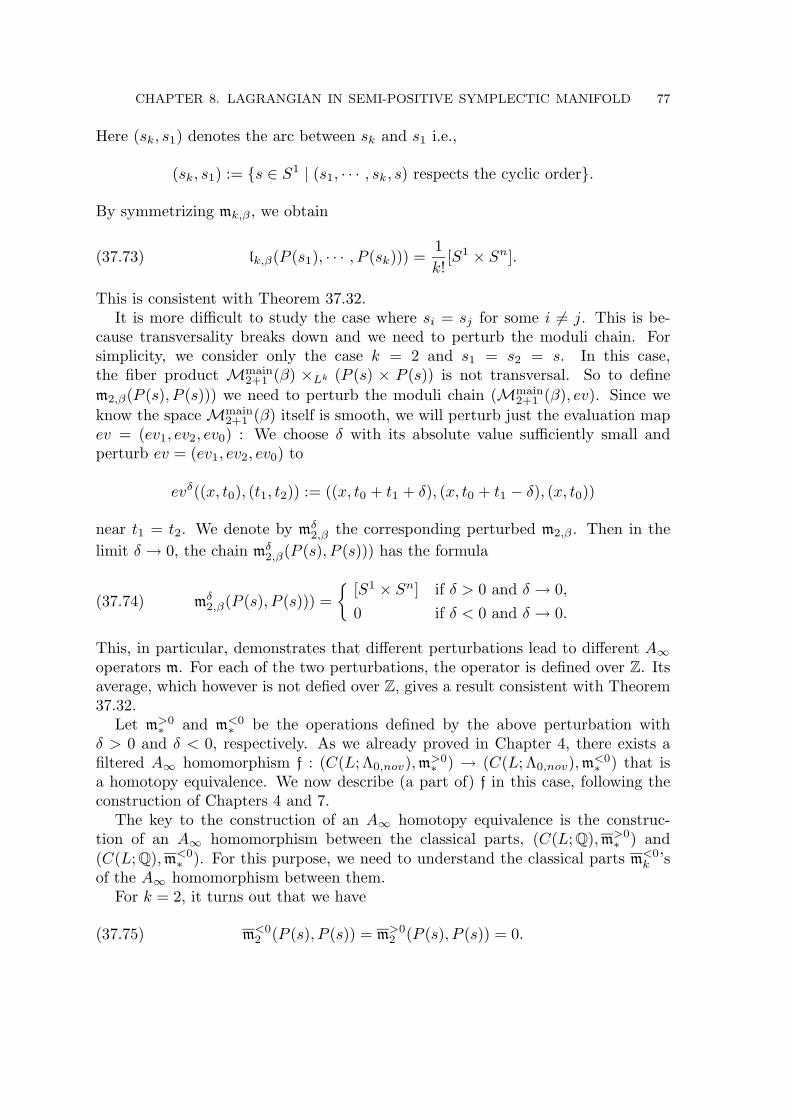
CHAPTER 8. LAGRANGIAN IN SEMI-POSITIVE SYMPLECTIC MANIFOLD 77
Here (sk, s1) denotes the arc between sk and s1 i.e.,
(sk, s1) := {s ∈ S1 | (s1, · · · , sk, s) respects the cyclic order}.
By symmetrizing mk,β , we obtain
(37.73) lk,β(P (s1), · · · , P (sk))) =1k!
[S1 × Sn].
This is consistent with Theorem 37.32.It is more difficult to study the case where si = sj for some i 6= j. This is be-
cause transversality breaks down and we need to perturb the moduli chain. Forsimplicity, we consider only the case k = 2 and s1 = s2 = s. In this case,the fiber product Mmain
2+1 (β) ×Lk (P (s) × P (s)) is not transversal. So to definem2,β(P (s), P (s))) we need to perturb the moduli chain (Mmain
2+1 (β), ev). Since weknow the space Mmain
2+1 (β) itself is smooth, we will perturb just the evaluation mapev = (ev1, ev2, ev0) : We choose δ with its absolute value sufficiently small andperturb ev = (ev1, ev2, ev0) to
evδ((x, t0), (t1, t2)) := ((x, t0 + t1 + δ), (x, t0 + t1 − δ), (x, t0))
near t1 = t2. We denote by mδ2,β the corresponding perturbed m2,β . Then in the
limit δ → 0, the chain mδ2,β(P (s), P (s))) has the formula
(37.74) mδ2,β(P (s), P (s))) =
Ω[S1 × Sn] if δ > 0 and δ → 0,
0 if δ < 0 and δ → 0.
This, in particular, demonstrates that different perturbations lead to different A1operators m. For each of the two perturbations, the operator is defined over Z. Itsaverage, which however is not defied over Z, gives a result consistent with Theorem37.32.
Let m>0∗ and m<0
∗ be the operations defined by the above perturbation withδ > 0 and δ < 0, respectively. As we already proved in Chapter 4, there exists afiltered A1 homomorphism f : (C(L;Λ0,nov),m>0
∗ ) → (C(L;Λ0,nov),m<0∗ ) that is
a homotopy equivalence. We now describe (a part of) f in this case, following theconstruction of Chapters 4 and 7.
The key to the construction of an A1 homotopy equivalence is the construc-tion of an A1 homomorphism between the classical parts, (C(L; Q),m>0
∗ ) and(C(L; Q),m<0
∗ ). For this purpose, we need to understand the classical parts m<0k ’s
of the A1 homomorphism between them.For k = 2, it turns out that we have
(37.75) m<02 (P (s), P (s)) = m>0
2 (P (s), P (s)) = 0.

78 FUKAYA, OH, OHTA, ONO
To see this, we recall the construction from §30 and the proof of (37.74). Weremark that the intersection P (s)∩P (s) = P (s) is not transversal since dimP (s) <dimL. Therefore we need to choose a suitable perturbation of the moduli chains todefine which led us to the perturbed chains m<0
2 (P (s), P (s)) and m>02 (P (s), P (s)).
The perturbations should be consistent with that of [Mmain2+1 (β), ev] given above :
More precisely speaking, we first perturb Mmain2+1 (β0) to define m<0
2 and then choosea perturbation of Mmain
2+1 (β) so that it is consistent with the definition of m<02,β .
Following the recipe in §30, we consider a pair of diffeomorphisms
(ϕ0,δ,ϕ1,δ) : L → L× L
given by(ϕ0,δ(t, x),ϕ1,δ(t, x)) = ((t + δ, x), (t− δ, x)).
Then according to §30.3 we have
m>02 (P (s), P (s)) = {p ∈ L | ϕ0,δ(p) ∈ P (s),ϕ1,δ(p) ∈ P (s)}
for δ > 0 and similarly for δ < 0. It easily follows that
m>02 (P (s), P (s)) = 0 = m<0
2 (P (s), P (s)).
Now to construct an A1 homomorphism
(C(L; Q),m>0∗ ) → (C(L; Q),m<0
∗ ),
we need to take a homotopy between the two perturbations, one corresponding to(ϕ0,δ,ϕ1,δ) and the other corresponding to (ϕ0,−δ,ϕ1,−δ) for δ > 0. The obviouschoice of such a homotopy is H : L× [−1, 1] → L× L defined by
(p, u) 7→ (ϕ0,uδ(p),ϕ1,uδ(p)).
By the definition of the map f2 which is induced by H, we obtain
f2(P (s), P (s)) = {p ∈ L |∃u ∈ [−1, 1], H(p, u) ∈ P (s)× P (s)}
which gives rise tof2(P (s), P (s)) = [P (s)].
Note we do not need to perturb moduli chain (Mmain1+1 (β), ev) to define the map
m1,β . This is because it follows from the formula (37.71) that the fiber product
Mmain1+1 (β)×L P

CHAPTER 8. LAGRANGIAN IN SEMI-POSITIVE SYMPLECTIC MANIFOLD 79
is always transversal for any chain P ⊂ L. In particular, this leads to the identitym>0
1,β = m<01,β and allows us to choose f1 = id for the map f1. We also derive
m1,β(P (s)) = [S1 × Sn]
from (37.71).Combining all these, we obtain the identities
(37.76)
m>02,β(f1(P (s)), f1(P (s)))
= m>02,β(P (s), P (s)) = [S1 × Sn]
= m1,β(f2(P (s), P (s))) + m<02,β(f1(P (s)), f1(P (s))).
The identity between the first line and the last in (37.76) is precisely the one requiredfor f to be a filtered A2 homomorphism modulo T 2.
37.6. Further study of Floer theory of S1 × Sn ⊂ Cn+1.
We next explain some ideas how one can improve the proofs of Theorems 37.30and 37.32 and obtain additional information on the integer ∏ given in (37.33) andothers.
We recall the definition of l+k+1,β from (37.26). The following information can beeasily read off from Lemma 37.41, 37.42 and 37.44.
Proposition 37.77. Let L ⊂ Cn+1 be a Lagrangian submanifold which is homeo-morphic to S1 × Sn. Then l+k+1,β ≡ 0 mod T 2 unless one of the following alterna-tives holds :
(1) µL(∞) = 2,(2) n is odd and µL(∞) = n + 1,(3) n is even and µL(∞) = 2− n.
Proof. When n = 1, the assertion is obvious. So we may assume that n 6= 1. Let∞ = @β ∈ π1(L) be the boundary class of β. Based on Proposition 37.38, it sufficesto show that ev∗([M0(β)]) ∈ HµL(∞)+n−2(L(L; ∞)/S1; Q) is zero otherwise.
Suppose to the contrary that ev∗([M0(β)]) is non-zero. According to Lemmas37.41, 37.42 and 37.44, the homology group Hm(L(L; ∞)/S1; Q) is nonzero only for
m = k(n− 1), or k(n− 1) + n for k ∈ Z≥0 when n is odd,
and
m = 0, (2` + 1)(n− 1), or 2`(n− 1) + n for ` ∈ Z≥0 when n is even.

80 FUKAYA, OH, OHTA, ONO
Therefore it is easy to see that one of the three possibilities must occur if µL(∞) +n−2 ≤ 2n−1. On the other hand if µL(∞)+n−2 > 2n−1, we have µL(∞) ≥ n+2: This has been already ruled out in Theorem 37.4. This finishes the proof. §
Possibilities (1), (2) are the cases discussed in Theorems 37.21 and 37.22 andindeed occur as shown in (37.1), (37.2) and Lemma 37.3. (Compare Remark 37.5also.)
The discussion in the rest of this section will be brief the details of which willbe treated elsewhere. We will study the first nonzero term of the l+k+1 particularlyfor the case where the homology class ev∗([M0(β)]) ∈ HµL(∞)+n−2(L(L; ∞)/S1; Q)is zero.
‘Proposition 37.78’. Suppose that n is odd and `µL(∞) = n + 1 with ` 6= 1, n+12 .
Then, we have :
(37.79) l+k+2(ak1 , an, an+1) ≡ ± 1
k!e(n+1)/2`kT ` mod T `+1.
Here the ± is independent of k. Moreover the left hand side is independent of thepermutation of the variables modulo T `+1. All the other operations are zero moduloT `+1.
We have the same conclusion when µL(∞) = 2 = (n+1)/` and l+k+1(ak1 , an+1) ≡ 0
mod T 2.
Sketch of the proof. We proved that ev∗([M0(β)]) ∈ HµL(∞)+n−2(L(L; ∞)/S1; Q) iszero in the course of the proof of Proposition 37.77 under the given hypotheseson µL(∞). We assume that ev∗([M0(β)]) is zero not only as a homology class butalso as a chain. Then by the same argument as the proof of Lemma 37.36, we canprove that M0(2β) is a manifold without boundary for a generic almost complexstructure. Its homology class lies in H2µL(∞)+n−2(L(L; ∞)/S1; Q) and hence is zeroby the degree reason, unless ` = 2. We assume that ev∗([M0(2β)]) is zero as achain. Using this assumption, we can continue. Then (under these assumptions)we find a manifold without boundary M0(`β) which represents a homology class inH2n−1(L(L; `∞)/S1; Q). This is because H∗(L(L; `∞)/S1; Q) = 0 for ∗ = n + 1, n +2, · · · , 2n− 2 and mµL(∞) + n− 2 ∈ {n + 2, n + 4, · · · , 2n− 2} for m = 1, · · · , `− 1.
Using M0(`β) we can repeat the proof of Theorem 37.30 and obtain the followingconclusion : Define ∏ by
(37.80) ev∗([M0(`β)]) = ∏I((x⊗ zn)∗).
(Compare this with (37.40) and (37.45).) We remark that in our case I : L(Sn) →L(L; `∞)/S1 is not a homotopy equivalence. (Compare Lemma 37.41). However itinduces an isomorphism on homology group over Q.
We first prove
(37.81) l+k+2(ak1 , an, an+1) ≡ ± ∏
k!e(n+1)/2`kT ` mod T `+1.

CHAPTER 8. LAGRANGIAN IN SEMI-POSITIVE SYMPLECTIC MANIFOLD 81
By the linearity, it suffices to consider the case ∏ = 1 in (37.80). Then we mayassume in addition that ev∗([M0(`β)]) is realized by P × S1 where P is a chain onL(Sn) as in the proof of Lemma 37.47. Then
evk+1 : M1(`β)× (S1)k+1 → (S1 × Sn)k+1
is given as
(37.82)evk+1((x, s), (t1, · · · , tk+1))= ((`x(t1), s + `t1), · · · , (`x(tk+1), s + `tk+1), (`x(1), s)).
We remark that (37.82) is slightly different from (37.50). Namely we have s + `tiin place of s+ ti in the right hand side. We use (37.82) to show (37.81) in the sameway as the proof of Lemma 37.47.
We next show ∏ = 1. This follows from l1(αn) = ∏e(n+1)/2T `a0 and Proposition37.15.
Therefore we have proved (37.79).Thus, the proof of Proposition 37.78 is finished under the assumptions mentioned
above. However one of the chainsM0(mβ) in HmµL(∞)+n−2(L(L;m∞)/S1; Q), whichis zero as a homology class, may be nonzero as a chain. Therefore to handle thefictitious assumptions in the above proof, we need to work everything in the chainlevel and to inductively find a sequence of chains on the loop space that boundsthe cycles ev∗([M0(mβ)]) for various m’s. This inductive argument is very similarto those presented in the earlier chapters of this book. The only difference is thatwe have constructed bounding chains as the chains on the manifold L itself in thisbook, while we now need to do a similar construction on the loop space of L. Anoutline of the details of this construction is given in [Fuk05II] and the full detailsthereof will be provided in [Fuk07]. §
We remark that ‘Proposition 37.78’ also implies that the sign in (37.17.1) coin-cides with sign in (37.17.2).
We next consider the case when n is even.
‘Proposition 37.83’. The possibility (37.12) does not occur.
Sketch of the proof. We prove this by contradiction. Suppose to the contrary that(37.12) occurs. Then, by the argument in the proof of Theorem 37.4, we haveδ2 = 0. This means that ev∗([M0(β)]) is zero as a homology class. We assumethat it is zero as a chain. Now we repeat the process similar to the sketch of theproof of ‘Proposition 37.78’ until we arrive in the first nontrivial homology classev∗([M0(mβ)]). On the other hand we have the formula (37.12),
δ(n)(n+2)/2(an) = ±a1

82 FUKAYA, OH, OHTA, ONO
which we proved under the assumption (37.12). This implies that the homologyclass ev∗([M0(((n + 2)/2 − 1)β)]) ∈ H2n−2(L(L; ∞)/S1; Q) is nonzero. This ishowever impossible since H2n−2(L(L; ∞)/S1; Q) = 0 by Lemmas 37.41, 37.42 and37.44 unless n = 2. (We remark that n is even in our situation. The nontrivialityof the differential in Lemma 37.44 plays a crucial role here.) In case that n = 2, wefind that H2(L(S! × S2; ∞)/S1; Q) ∼= H2(L(S2); Q) is generated by 1 ⊗ z2. We canuse it to show that m1,β(an) = 0 again. The current proof is incomplete becauseof the same reason as that of ‘Proposition 37.78’ is. (But it is rigorous in casen = 2.) §
‘Proposition 37.84’. When n is even, ∏ in Theorem 37.32 satisfies ∏ = ±1.
Proof. By ‘Proposition 37.83’ and Proposition 37.10, we have δ(1)2 (a1) = ±a0. This
implies ∏ = ±1 in Theorem 37.32. §
§38. Anti-symplectic involutions.
In the rest of this chapter we work in the following situation. Let (M,ω) bea compact symplectic manifold. An involution τ of (M,ω) is assumed to be anti-symplectic. Namely we assume
(38.1) τ∗(ω) = −ω.
We also assume that the fixed point set L = Fix τ of τ is non-empty. It is theneasy to see that L is a Lagrangian submanifold.
Let Jω be the set of all ω compatible almost complex structures, and J τω be its
subset consisting of almost complex structures J satisfying
(38.2) τ∗J = −J.
Such an almost complex structure J is said to be τ -anti-invariant.
Lemma 38.3. The space J τω is non-empty and contractible. It becomes an infinite
dimensional (Frechet) manifold.
Proof. For given J ∈ J τω , its tangent space TJJ τ
ω consists of sections Y of the bundleEnd(TM) whose fiber at p ∈ M is the space of linear maps Y : TpM → TpM suchthat
Y J + JY = 0, ω(Y v,w) + ω(v, Y w) = 0, τ∗Y = −Y.

CHAPTER 8. LAGRANGIAN IN SEMI-POSITIVE SYMPLECTIC MANIFOLD 83
Note that the second condition means that JY is a symmetric endomorphism withrespect to the metric gJ = ω(·, J ·). It immediately follows that J τ
ω becomes amanifold. The fact that J τ
ω is non-empty (and contractible) follows from the polardecomposition theorem by choosing a τ -invariant Riemannian metric on M . §
We recall Definition 5.17 where we introduce the Γ-equivalence relation ∼ andthe quotient group
Π(L) = π2(M,L)/ ∼
which is abelian. Then for each β ∈ Π(L), we defined the moduli space M(J ;β) asthe union [
B∈β⊂π2(M,L)
M(J ;B).
We also recall that Mk+1,m(J ;β) is the set of all bordered stable maps of genuszero representing the class β with k + 1 boundary and m interior marked points.Let Mreg
k+1,m(J ;β) be its subsets consisting of all elements [((Σ,~z,~z+), w)] such thatΣ = D2. Here ~z = (z0, · · · , zk) are boundary marked points, and z+
1 , · · · , z+m are
interior marked points. (See Definition 2.27.)We now go back to our discussion. Let J ∈ J τ
ω . For a J holomorphic curvew : (D2, @D2) → (M,L), u : S2 → M , we define ew, eu by
(38.4) ew(z) = (τ ◦ w)(z), eu(z) = (τ ◦ u)(z).
For [(D2, w)] ∈Mreg(J ;β), [((D2,~z,~z+), w)] ∈Mregk+1,m(J ;β) we define
(38.5) τ∗([(D2, w)]) = [(D2, ew)], τ∗([((D2,~z,~z+), w)]) = [((D2,~z,~z+), ew)],
where~z = (z0, · · · , zk), ~z
+= (z+
0 , · · · , z+m).
For β = [w], we put τ∗β = [ ew]. Note if τ] : π2(M,L) → π2(M,L) is the homomor-phism induced by τ then τ∗β = −τ]β. This is because z 7→ z is of degree −1. Infact we have
τ∗(β) = β
on Π(L), since τ∗ preserves both energy and Maslov index.
Lemma 38.6. The definition (38.5) induces the maps
τ∗ : Mreg(J ;β) →Mreg(J ;β), τ∗ : Mregk+1,m(J ;β) →Mreg
k+1,m(J ;β).
Proof. If (w, (z0, · · · , zk), (z+1 , · · · , z+
m)) ∼ (w0, (z00, · · · , z0k), (z0+1 , · · · , z0+m )), then thereexists ϕ ∈ PSL(2, R) = Aut(D2) such that w0 = w ◦ ϕ−1, z0i = ϕ(zi), z0+i = ϕ(z+
i ).

84 FUKAYA, OH, OHTA, ONO
We put ϕ(z) = (ϕ(z)). Then ϕ ∈ PSL(2, R) and ew0 = ew ◦ ϕ−1, z0i = ϕ(zi),z0+i = ϕ(z+
i ). §
We remark that the mapping ϕ 7→ ϕ, PSL(2, R) → PSL(2, R) is orientationpreserving.
In §44.1 Chapter 9, we will show that a choice of relative spin structure on Linduces an orientation on Mk+1,m(L;β) for any given β ∈ Π(L). Hereafter we usethis orientation to regard Mk+1,m(L;β) being oriented as a space with Kuranishistructure.
The notion of the group action on the space with Kuranishi structure is definedin §A1.3 Definition A1.45.
Proposition 38.7. Let J ∈ J τω . The map τ∗ : Mreg(J ;β) →Mreg(J ;β) induces
an involution of the space with Kuranishi structure. It is orientation preserving ifµL(β) ≡ 0 mod 4 and is orientation reversing if µL(β) ≡ 2 mod 4.
We will prove this proposition in §47.2 (Chapter 9). Here we give some examples.
Example 38.8. (1) Consider the case of M = CPn, L = RPn. In this case, eachMaslov index µL(β) has the form
µL(β) = `β(n + 1)
where β = `β times the generator. We know that when n is even L is not orientable,and so we consider only the case where n is odd. On the other hand, when n isodd, L is relatively spin : The class st will be the generator of H2(CPn; Z2), whichis preserved by τ if and only if n is odd. Hence L is τ -relatively spin if n is odd.Using the above formula for the Maslov index, we conclude from Proposition 38.7that the map τ∗ : Mreg(J ;β) →Mreg(J ;β) is orientation preserving if and only if`β is even.
(2) Let M be a Calabi-Yau 3-fold and L ⊂ M be the set of real points (i.e.,the fixed point set of an anti-holomorphic involutive isometry). In this case, L isorientable (because it is a special Lagrangian) and spin (because any orientable3-manifold is spin). Furthermore µL(β) = 0 for any β ∈ π2(M,L). ThereforeProposition 38.7 implies that the map τ∗ : Mreg(J ;β) →Mreg(J ;β) is orientationpreserving.
We next include markings. We consider the moduli space Mregk+1,m(J ;β).
Lemma 38.9. τ∗ : Mregk+1,m(J ;β) → Mreg
k+1,m(J ;β) induces an involution of thespace with Kuranishi structure. It is orientation preserving if and only if µL(β)/2+k + 1 + m is even.

CHAPTER 8. LAGRANGIAN IN SEMI-POSITIVE SYMPLECTIC MANIFOLD 85
Proof. The first half follows immediately from Proposition 38.7. To prove the secondhalf we consider the diagram :
(S1)k+1 × (D2)m c−−−−→ (S1)k+1 × (D2)m
inclusion
x inclusion
x
((S1)k+1 × (D2)m)0c−−−−→ ((S1)k+1 × (D2)m)0
yy
fMregk+1,m(J ;β) Lemma 38.9−−−−−−−→ fMreg
k+1,m(J ;β)
forget
y forget
y
fMreg(J ;β) Proposition 38.7−−−−−−−−−−→ fMreg(J ;β)
Diagram 38.1.
Here c is defined by c(z1 · · · , zk, z+1 , · · · , z+
m, z0) = (z1, · · · , zk, z+1 , · · · , z+
m, z0) andforget are the forgetful maps of marked points. ((S1)k+1 × (D2)m)0 is the set of allc(z1 · · · , zk, z+
1 , · · · , z+m, z0) such that zi 6= zj , z+
i 6= z+j for i 6= j.
Lemma 38.9 then follows from Proposition 38.7 and the fact that Z2 action ofPSL(2, R) is orientation preserving. §
We will next extend τ∗ to the compactification and define a continuous map
(38.10) τ∗ : Mk+1,m(J ;β) →Mk+1,m(J ;β).
Proposition 38.11. The map τ defined on Mregk+1,m(J ;β) extends to a map τ∗ as
in (38.10). It can be regarded as an involution on the space with Kuranishi structure.It preserves orientation if and only if µL(β)/2 + k + 1 + m is even.
Proof. We define τ∗ by a double induction over E(β) and k. Namely we define anorder on the set of triples (β, k,m) by the relation
(38.12.1) E(β0) < E(β).(38.12.2) E(β0) = E(β), k0 < k.
With respect to this order, we will define the map (38.10) for (β, k,m) under theassumption that the map is already defined for all (β0, k0,m0) smaller than (β, k,m).
Let [((Σ,~z,~z +), w)] ∈Mk+1,m(J ;β). We first assume that Σ has a sphere bubbleS2 ⊂ Σ. We remove it from Σ to obtain Σ0. We add one more marked point to Σ0
at the location where the sphere bubble used to be attached. We then obtain anelement
[((Σ0,~z,~z(0)), w0)] ∈Mk+1,m+1−`(J ;β0).

86 FUKAYA, OH, OHTA, ONO
Here ` is the number of marked points on S2. By the induction hypothesis, τ∗ isalready defined on Mk+1,m+1−`(J ;β0) since E(β) > E(β0). We denote
τ∗([((Σ0,~z,~z(0)), w0)]) = [((Σ00,~z0,~z(0)0), w00)].
We define v|S2 : S2 → M byv(z) = w|S2(z).
We assume that the singular point of S2, i.e., the point in Σ0 ∩ S2 corresponds to0 ∈ C∪ {1} ∼= S2. We also map ` marked points on S2 by z 7→ z whose images wedenote by ~z(1) ∈ S2. We then glue ((S2,~z(1)), ew) to ((Σ00,~z 0,~z(0)0), ew) at the point0 ∈ S2 and at the last marked point of (Σ0,~z,~z(0)) and obtain a curve which is tobe the definition of τ∗([((Σ,~z,~z +), w)]).
Next suppose that there is no sphere bubble on Σ. Let Σ0 be the componentcontaining the 0-th marked point. If there is only one irreducible component ofΣ, then τ∗ is already defined there. So we assume that there is at least one disccomponent other than Σ0. Then Σ is a union of Σ0 and Σi for i = 1, · · · ,m (m ≥ 1).We regard the unique point in Σ0∩Σi for i = 1, · · · ,m as marked points of Σ0. Hereeach of Σi itself is a union of disc components and is connected. We also regard thepoint in Σ0 ∩Σi as 0 ∈ D2 ∼= H∪ {1} where D2 is the irreducible component of Σi
joined to Σ0, and also as one of the marked points of Σi. This defines an element[((Σi,~z(i),~z (i)+), w(i))] for each i = 0, · · · ,m. By an easy combinatorics and theinduction hypothesis, we can show that τ∗ is already constructed on them. Now wedefine τ∗([((Σ,~z,~z +), w)]) by gluing τ∗([((Σi,~z(i),~z (i)+), w(i))]).
We next consider Kuranishi structure on a neighborhood around the elementτ∗([((Σ,~z,~z +), w)]) in Mk+1,m(J ;β). We first observe that the map u 7→ eu on themoduli space of spheres defined in (38.4) can be regarded as an involution on thespace with Kuranishi structure, in the same way as the proof of Proposition 38.7.Then we can show that (38.10) induces a map of the space with Kuranishi structureby the same induction process as its construction. More precisely, we will proveexistence of an involution for Mk+1,m(J ;β) assuming that τ∗ induces involutionson spaces with Kuranishi structures onMk+1,m+1−`(J ;β0) for all (β0, k0,m0) smallerthan (β, k,m).
Let [((Σ,~z,~z +), w)] ∈Mk+1,m(J ;β). If it is in Mregk+1,m(J ;β), we have defined
an involution on its Kuranishi neighborhood in Proposition 38.7. If Σ is not irre-ducible, then [((Σ,~z,~z +), w)] is obtained by gluing some elements correspondingto (β0, k0,m0) < (β, k,m). For each irreducible component, the involution of itsKuranishi neighborhood is constructed by the induction hypothesis. A Kuranishineighborhood of [((Σ,~z,~z +), w)] is a fiber product of the Kuranishi neighborhoodsof the gluing pieces and the space of the smoothing parameters of the singularpoints. By definition, our involution obviously commutes with the process to takethe fiber product. For the parameter space smoothing the interior singularities, theaction of the involution is the complex conjugation. For the parameter space of

CHAPTER 8. LAGRANGIAN IN SEMI-POSITIVE SYMPLECTIC MANIFOLD 87
smoothing boundary singularities, the action of involution is trivial. The analysiswe worked out in §29 of the gluing is obviously compatible with the involution.Thus τ∗ defines an involution on Mk+1,m(J ;β) with Kuranishi structure.
The statement on the orientation follows from the corresponding statement onMreg
k+1,m(J ;β). §
We next restrict our maps to the main component of Mk+1,m(J ;β). We remarkthat τ∗ : Mk+1,m(J ;β) → Mk+1,m(J ;β) does not preserves the main componentfor k > 1. On the other hand the assignment given by
(38.13) (w, (z1, z2, · · · , zk−1, zk, z0)) 7→ ( ew, (zk, zk−1, · · · , z2, z1, z0))
respects the counter-clockwise cyclic order of S1 = @D2 and so preserves the maincomponent, where ew is as in (38.4). Therefore we consider this map instead whichwe denote by
τmain∗ : Mmain
k+1 (J ;β) →Mmaink+1 (J ;β).
Lemma 38.14. The map τmain∗ defines an involution of the space with Kuranishi
structure.
The proof is the same as the proof of Propositions 38.7 and 38.11 and so omitted.We now have the following commutative diagram,
(S1)k+1 × (D2)m c0−−−−→ (S1)k+1 × (D2)m
inclusion
x inclusion
x
((S1)k+1 × (D2)m)00c0−−−−→ ((S1)k+1 × (D2)m)00
yy
fMmaink+1 (J ;β)
τmain∗−−−−→ fMmain
k+1 (J ;β)
forget
y forget
y
fM(J ;β) τ∗−−−−→ fM(J ;β)
Diagram 38.2.
where c0 is defined by c0(z1 · · · , zk, z+1 , · · · , z+
m, z0) = (zk, · · · , z1, z+1 , · · · , z+
m, z0)and forget are the forgetful maps of marked points. ((S1)k+1 × (D2)m)00 is theopen subset of (S1)k+1 × (D2)m consisting of the points such that all zi’s and z+
j ’sare distinct respectively.
Let Revk : Lk+1 → Lk+1 be the map defined by
Revk(x1, · · · , xk, x0) = (xk, · · · , x1, x0).

88 FUKAYA, OH, OHTA, ONO
It is easy to see that
(38.15) ev ◦ τ∗ = Revk ◦ ev.
We remark that Revk = id, and τmain∗ = τ∗ for k = 0, 1.
Let P1, · · · , Pk be chains on L. By taking the fiber product and using (38.13) weobtain an involution
(38.16) τmain∗ : Mmain
k+1 (J ;β;P1, · · · , Pk) →Mmaink+1 (J ;β;Pk, · · · , P1).
We put≤ = µL(β)/2 + k + 1 +
X
1≤i<j≤k
deg0 Pi deg0 Pj .
Lemma 38.17. The involution (38.16) preserves orientation if ≤ is even, and re-verses orientation if ≤ is odd.
The proof of Lemma 38.17 is in §47.2 (Chapter 9).
Now we are ready to give the proofs of Theorem 34.20 and Proposition 34.25.
Proof of Theorem 34.20. We can take a system of multi-sections s onMmain
k+1 (J ;β;P1, · · · , Pk) which is preserved by (38.16). This is possible since (38.16)is an automorphism of order 2. (Namely we take quotient by Lemma A1.49, takea perturbed multi-section of the quotient, and lift it.) Theorem 34.20 then is animmediate consequence of the definition of the operator mk and Lemma 38.17. (Weremark that there may be a fixed point of (38.16). But this does not cause anyproblem as far as we work with multi-section and study virtual fundamental chainover Q.) §
Proof of Proposition 34.25. Let (N,ω) be a symplectic manifold, M = N ×N , andωM = ωN⊕(−ωN ). We consider τ : M → M , τ(x, y) = (y, x). Then L = N = Fix τ .Let JN be a compatible almost structure on N , and JM = JN ⊗ 1 − 1 ⊗ JN . Thealmost complex structure JM is compatible with ωM . Let v : S2 → N be a JN -holomorphic map. We fix 3 marked points 0, 1,1 ∈ S2 = C ∪ {1}. Then weconsider the upper half plane H ⊂ {1} ⊂ C∪{1} and define the map I(v) : H → Mby
I(v)(z) = (v(z), v(z)).
Identifying (H, (0, 1,1)) with (D2, (−1, 1,√−1)) with (−1, 1,
√−1) ∈ @D2, we ob-
tain a map from (D2, @D2) to (M,N) which we also denote by I(v). One caneasily check the converse : for any given map JM -holomorphic w : (D2, @D2) ∼=(H, R ∪ {1}) → (M,N) = (N ×N,∆N ), the assignment
v(z) =Ω
w(z) for z ∈ Hτ ◦ w(z) for z ∈ C with z ∈ H

CHAPTER 8. LAGRANGIAN IN SEMI-POSITIVE SYMPLECTIC MANIFOLD 89
defines a JN -holomorphic sphere on N . Therefore the map v 7→ I(v) gives an iso-morphism between the moduli spaces of JN -holomorphic spheres and JM -holomorphicdiscs with boundary in N . We can easily check that it is induced by the isomorphismof Kuranishi structures. Proposition 34.25 follows. §
Proof of Theorem N. Let L be as in Theorem N. By Theorem 34.20 we have
m0,β(1) = −m0,β(1) = 0
for all β ∈ Π(L) and hence M(L; Q) 6= ∅.On the other hand, c1(M) = 0 implies µL = 0. (Recall that L = Fix τ .)
Therefore the conclusion follows from Theorem 24.21. §
§39. Generic invariant almost complex structure and semi-positivity.
In this section we show that for L = Fix τ the transversality result in Chapter 7and §35 can be proved using only the τ -anti-invariant J ’s :
τ∗J = −J.
We first prove the following proposition.
Proposition 39.1. Let M be a semi-positive symplectic manifold with an anti-symplectic involution τ . Then there exists a τ anti-invariant compatible almostcomplex structure J , such that every J-holomorphic sphere v : S2 → M satisfiesc1(M) ∩ [v] ≥ 0.
Proof. For the proof we need some notations. Let J ∈ J τω .
Definition 39.2. A J-holomorphic sphere v : S2 → M is said to be τ -somewhereinjective if there exists z ∈ S2 such that
(39.3.1) v is an immersion at z,(39.3.2) v(z) /∈ v(S2\{z}),(39.3.3) v(z) /∈ τ(v(S2)).
Let w : (D2, @D2) → (M,L) a J-holomorphic disc. We say that it is τ -somewhereinjective if there exists z ∈ Int D2 such that
(39.4.1) w is an immersion at z,(39.4.2) w(z) /∈ w(D2\{z}),(39.4.3) w(z) /∈ τ(w(D2)).

90 FUKAYA, OH, OHTA, ONO
Let v : S2 → M be a J-holomorphic sphere and w : (D2, @D2) → (M,L) aJ-holomorphic disc. Recalling the definition of the non-linear Cauchy-Riemannoperator denoted by @, we consider its linearizations along the map-direction(39.5) Dv@ : Γ(S2, v∗TM) → Γ(S2,Λ0,1 ⊗ v∗TM)and(39.6) Dw@ : Γ((D2, @D2), (w∗TM,w|∗@D2(TL))) → Γ(D2,Λ0,1 ⊗ w|∗@D2TM).Lemma 39.7. For generic J ∈ J τ
ω , (39.5) is surjective for any τ -somewhere in-jective sphere v and (39.6) is surjective for all τ -somewhere injective disc w.
Proof. The proof is a minor modification of that of [McD87]. Let v : S2 → M be aτ -somewhere injective J-holomorphic sphere. By considering the linearization of @along the J-direction, we obtain a linear map
DJ@ : TJJ τω → Γ(S2,Λ0,1 ⊗ v∗TM).
To prove the first half of the statement, it suffices to showΓ(S2,Λ0,1 ⊗ v∗TM) = Im Dv@ + Im DJ@
where the right hand side is the same as the image of the total linearization of @ at(v, J).
Let z ∈ S2 be a point as in (39.3). Then we can choose a small neighborhood Wof v(z) in M such that
W ∩ τ(W ) = ∅and a small neighborhood U of z in S2 that satisfies
W ∩ v(S2 \ U) = ∅, W ∩ τ(v(S2)) = ∅.Denote by Jω(W ) the set of all compatible almost complex structures J 0 that coin-cide with J outside W . (Note that elements of Jω(W ) may not be τ -anti-invariant.)Then it follows from [McD87] that
(39.8) (DJ@)(TJJω(W )) + Im(Dv@) = Γ(S2,Λ0,1 ⊗ v∗TM).We define a map S : Jω(W ) → J τ
ω by putting
S(J 0) =Ω −τ∗(J 0) on τ(W ),
J 0 outside τ(W )for J 0 ∈ Jω(W ). Using the property W ∩ τ(W ) = ∅ of W , we can easily checkthat S(J 0) is τ -anti-invariant. On the other hand, it follows from the propertyτ(W ) ∩ v(S2) = ∅ that DJ@ ◦DS = DJ@ at (v, J). Therefore
(DJ@)(TJJω(W )) ⊂ (DJ@)(TJJ τω ).
Combining this with (39.8), we have proved
(DJ@)(TJJ τω ) + Im(Dv@) = Γ(S2,Λ0,1 ⊗ v∗TM)
which is precisely what we wanted to prove. This finishes the proof for the spheresv. The argument for τ -somewhere injective discs is similar and omitted. §

CHAPTER 8. LAGRANGIAN IN SEMI-POSITIVE SYMPLECTIC MANIFOLD 91
Remark 39.9. McDuff proved that every J-holomorphic sphere is a branchedcovering of somewhere injective sphere [McD87]. On the other hand, if we definesomewhere injectivity of J-holomorphic disc by (39.4.1) and (39.4.2), then it is notthe case in general that every J-holomorphic disc is branched covering of a some-where injective disc. While analyzing the structure of the image of J-holomorphicdiscs requires more delicate study given as in [KwOh00] (see [Lazz00] also), we donot need the deep structure theorem in the proof of Proposition 39.1.
Now we go back to the proof of Proposition 39.1. Let us take a compatiblealmost complex structure satisfying the conclusion of Lemma 39.7. Then the semipositivity of M implies that there exists no τ -somewhere injective J-holomorphicsphere v : S2 → M with c1(M)([v]) < 0 obviously because τ -somewhere injectivityimplies somewhere injectivity. Note that in general J-holomorphic sphere is notnecessarily a branched covering of τ -somewhere injective one. So we need somemore argument to prove Proposition 39.1.
Let v : S2 → M be a J-holomorphic sphere satisfying c1(M)([v]) < 0. Then vcannot be τ -somewhere injective by Lemma 39.7 and by the semi-positivity of M . Ifv is not somewhere injective either, we can find a somewhere injective sphere v suchthat v is a (branched) covering of v. Evidently we have c1(M)([v]) < 0. Therefore,replacing v by v if necessary, we may and will assume that v : S2 → M is somewhereinjective. However v itself may not be necessarily τ -somewhere injective.
Since v is somewhere injective, it is immersed away from a finite number of pointsin S2. On the other hand, since it is not τ -somewhere injective, it follows that
τ(v(S2)) = v(S2).
Therefore τ : M → M induces an involution
eτ : S2 → S2
by the formulav ◦ eτ = τ ◦ v.
Using the immersion property of v, one can check that eτ is smooth. Furthermoreit also satisfies Teτ ◦ j = −j ◦ Teτ , i.e., eτ defines an anti-holomorphic involution onS2. (In this section we denote by Tf the differential of a map f .)
We consider the linearization map along the v-direction
(39.10) Dv@ : Γ(S2, v∗TM) → Γ(S2,Λ0,1 ⊗ v∗TM).
Using τ and eτ , we define an involution I on Γ(S2, v∗TM) by
(39.11.1) (I(u))(z) = (T τ)−1(u(eτ(z))).

92 FUKAYA, OH, OHTA, ONO
An involution I on Γ(S2,Λ0,1 ⊗ v∗TM) is also defined by
(39.11.2) (I(α))(z) = (T τ)−1 ◦ α(eτ(z)) ◦ Teτ ,
where α(z) ∈ (Λ0,1 ⊗ v∗TM)z is regarded as an anti-complex linear map : TzΣ →Tv(z)M .
It is easy to see that Dv@ commutes with I. Let
Γ(S2, v∗TM) = Γ(S2, v∗TM)+ ⊕ Γ(S2, v∗TM)−
be the decomposition of Γ(S2, v∗TM) according to the I-invariant and I-anti-invariant parts. We define Γ(S2,Λ0,1⊗v∗TM)± in a similar way. Then the complex(39.10) splits into
(39.12.1) (Dv@)+ : Γ(S2, v∗TM)+ → Γ(S2,Λ0,1 ⊗ v∗TM)+,
(39.12.2) (Dv@)− : Γ(S2, v∗TM)− → Γ(S2,Λ0,1 ⊗ v∗TM)−.
Lemma 39.13.Index(Dv@)+ = Index(Dv@)−.
Here Index stands for the real index.
Proof. J induces isomorphisms on Γ(S2, v∗TM) and Γ(S2,Λ0,1 ⊗ v∗TM) by u 7→J ◦ u and α 7→ J ◦α, respectively. (Here we are using the notations of (39.11).) Wedenote them also by J . It is easy to see from (39.11) and the definition of J thatIJ = −JI. Hence J exchanges Γ(S2,Λ0,1 ⊗ v∗TM)+ and Γ(S2,Λ0,1 ⊗ v∗TM)−.
Moreover J commutes with the symbol of the operator Dv@. (Note J may notcommutes with Dv@.) The lemma then follows from the fact that the index dependsonly on the symbol. §
Now we prove the following lemma.
Lemma 39.14. For a generic element J of J τω , the operator (39.12.1) is surjective
for any somewhere injective sphere v (which may not necessarily be τ -somewhereinjective).
Proof. The lemma follows from Lemmas 39.7 and 39.13, if v is τ -somewhere injec-tive. Therefore it remains to consider the case where v is not τ -somewhere injective.Then there exists an anti-holomorphic involution eτ : S2 → S2 defined by τ ◦v = v◦eτas before. This induces the splitting
Γ(S2,Λ0,1 ⊗ v∗TM) = Γ(S2,Λ0,1 ⊗ v∗TM)+ ⊕ Γ(S2,Λ0,1 ⊗ v∗TM)−

CHAPTER 8. LAGRANGIAN IN SEMI-POSITIVE SYMPLECTIC MANIFOLD 93
corresponding to the eigenspaces of I with the eigenvalue ±1. Using the samenotation as in the proof of Lemma 39.7, we consider the linearization of @ in theJ-direction
DJ@ : TJJ τω → Γ(S2,Λ0,1 ⊗ v∗TM).
We denote by (DJ@)+ the projection of DJ@ with respect to the above splitting. Itnow suffices to show
(39.15) (DJ@)+(TJJ τω (W )) + Im((Dv@)+) = Γ(S2,Λ0,1 ⊗ v∗TM)+
by a similar reason as for (39.8). By the somewhere injectivity of v, we have a pointz ∈ S2 that satisfies (39.3.1) and (39.3.2) ( but not necessarily (39.3.3)). By slightlymoving z, we may assume that z is not a fixed point of eτ . Then we can choose anopen neighborhood U of z such that eτ(U) ∩ U = ∅. We also choose an open subsetW of M such that v(U) ⊂ W and τ(W ) ∩W = ∅. Again we have (39.8).
We now recall the set Jω(W ) and the map S : Jω(W ) → J τω defined in the end
of the proof of Lemma 39.7. We will now prove
(39.16) (DJ@)+ ◦DS = (DJ@)+
at (v, J). Let δJ ∈ TJ(Jw(W )) ⊆ Γ(W,EndR(TM)). Then we have
(39.17) (DS)(δJ)τ(p) = −(T τ)−1 ◦ δJ(p) ◦ T τ
for p ∈ W ⊂ M . On the other hand, from the definition
(39.18) @v =12(Tv + J ◦ Tv ◦ j)
we have the formula
(39.19) (DJ@)(δJ) =12δJ ◦ Tv ◦ j
for δJ ∈ TJJw ⊂ Γ(M,EndR(TM)). Combining j ◦Teτ = −Teτ ◦j, (39.11.2), (39.17)and (39.19), we derive
(I ◦DJ@ ◦DS)(δJ)(z)
=12(T τ)−1 ◦DS(δJ)eτ(z) ◦ Tv ◦ j ◦ Teτ
=12DS(δJ)p ◦ (T τ)−1 ◦ Tv ◦ Teτ ◦ j.
By differentiating τ−1 ◦ v ◦ eτ = v, we show that the last term becomes 12DS(δJ)p ◦
Tv ◦ j from which we conclude
(I ◦DJ@ ◦DS)(δJ) = (DJ@ ◦DS)(δJ)

94 FUKAYA, OH, OHTA, ONO
at (v, J). Projecting this identity to the eigenspace Γ(S2,Λ0,1⊗v∗TM)+ of I (witheigenvalue 1), the identity (39.16) follows.
Then (39.16) and (39.8) imply (39.15) which finishes the proof of Lemma 39.14. §
Now we assume that J satisfies the conclusion of Lemma 39.14 and Lemma39.7. We now wrap up the proof of Proposition 39.1 by showing that for such JProposition 39.1 holds. Suppose to the contrary c1(M)[v] < 0 for a J-holomorphicv. By the semi-positivity of M , this implies
c1(M)([v]) < 3− n or c1(M)([v]) + n < 3.
By taking Lemma 39.13 into account, this implies that the real index of the operator(39.12.1), which is given by c1(M)([v]) + n, is less than 3.
On the other hand, since Lemma 39.14 shows that the operator (Dv@)+ at vis surjective by the choice of J , c1(M)([v]) + n is the actual real dimension of theτ -invariant part of the moduli space containing v. There are two cases for therestriction of τ to the domain of v. Namely, the reflection along the equator or theantipodal map. In the first case, the group of automorphisms of CP 1 commutingwith the reflection is isomorphic to PSL(2; R). In the second case, the group ofautomorphisms commuting with the antipodal map is SO(3). In both cases, theautomorphism group is real 3-dimensional. Since v is non-constant, the actualdimension of the τ -invariant part of the moduli space must be at least greater thanequal to 3, which gives rise to a contradiction. The proof of Proposition 39.1 is nowcomplete. §
Corollary 39.20. Let M be a semi-positive symplectic manifold with anti sym-plectic involution τ . Let L = Fix τ . Then there exists J ∈ J τ
ω , such that everyJ-holomorphic disc w : (D2, @D2) → (M,L) satisfies µL([w]) ≥ 0.
Proof. We choose J satisfying the conclusion of Proposition 39.1. Let w : (D2, @D2) →(M,L) be a J-holomorphic disc. We consider its double v : S2 → M , which is aJ-holomorphic sphere. Proposition 39.1 implies c1(M)[v] ≥ 0. On the other hand,a simple topological calculation proves the gluing formula
2c1(w1#w2) = µL(w1) + µL(w2)
for two discs wi : (D2, @D2) → (M,L), i = 1, 2 satisfying w1|@D2 = w2|@D2 . Herew2 denotes the obvious map induced by w2 which is defined on the lower hemi-sphere by considering the reflection along the equator of S2. (See [Vit87] for itsproof.) On the other hand, when L = Fix τ and w1 = w and w2 = ew, this reducesto c1(M)[v] = µL([w]) because we have µL([w]) = µL([ ew]). Therefore Proposition39.1 implies µL([w]) ≥ 0. §
By the proof of Theorems 34.11, we can use the almost complex structure Jsatisfying the conclusion of Proposition 39.1 and Corollary 39.20, and an abstract

CHAPTER 8. LAGRANGIAN IN SEMI-POSITIVE SYMPLECTIC MANIFOLD 95
perturbation (that is, a perturbation of the Kuranishi map) to obtain the filtered A1algebras mentioned in Theorems 34.4 and 34.7. However to apply the cancellationargument, we still need to construct a τ∗-invariant perturbation s≤. When τ∗ doesnot have a fixed point, such construction is easy to carry out. However, since τ∗ mayhave a fixed point in general, it is not a trivial matter to construct a τ∗-invariant(abstract) perturbation s≤ so that the τ -invariant version of Theorem 34.11 holds.We will resolve this trouble in the next four sections.
§40. Lantern.
Let J be an almost complex structure of M that we fixed at the end of the lastsection and β ∈ Π(L). Hereafter we will write Mmain
k+1 (β) in place of Mmaink+1 (J ;β).
We are going to study
(40.1) τ∗ : Mmaink+1 (β) →Mmain
k+1 (τ∗β) = Mmaink+1 (β), (k = 0, 1)
defined in (38.5) where we recall
β = τ∗β in Π(L).
In the rest of this chapter, we omit the symbol “main” since there is only onecomponent for k = 0, 1. In this section we study the fixed point set of τ∗.
We first consider M2(β). In this section we consider its subset Mreg2 (β). Here
Mregk+1(β) is a subset of Mk+1(β) consisting of elements [((Σ,~z), w)] such that Σ =
D2. (Namely it consists of the elements without bubble.)To study the fixed point set of τ∗, we construct a map
D : Mreg2 (β) →Mreg
2 (β + τ∗β) = Mreg2 (2β).
Let ((D2, (z0, z1)), w) represent an element [((D2, (z0, z1)), w)] of Mreg2 (β). By re-
quiring z0 = 1, z1 = −1, the representative ((D2, (1,−1)), w) is uniquely determinedmodulo the action of Aut(D2; 1,−1) which is isomorphic to R.
Denote the upper and lower semi-discs by
D2± = {z ∈ D2 | ± Im z ≥ 0}.
We take a conformal isomorphism ρ+ : D2+ → D2 such that ρ+(±1) = ±1 and
define the conformal isomorphism ρ− : D2− → D2 by ρ−(z) = (ρ+(z)).

96 FUKAYA, OH, OHTA, ONO
Now for a given w : (D2, @D2) → (M,L) with L = Fix τ , we define another mapew : (D2, @D2) → (M,L)
(40.2) ew(z) =
(w(ρ−(z)) if z ∈ D2
−,
(τ ◦ w)≥ρ+(z)
¥if z ∈ D2
+
by gluing w and τ ◦ w. Using this gluing, we define the map D by
(40.3) D([((D2, (1,−1)), w)]) = [((D2, (1,−1)), ew)].
We like to remark that we have given the definition of D only for the regularelements [((Σ, (z0, z1)), w)] i.e., on Mreg
2 (β).
Lemma 40.4. The definitions (40.2) and (40.3) give a well-defined map
D = Dβ : Mreg2 (β) →Mreg
2 (2β).
D is independent of the choice of ρ+. Moreover D satisfies
(40.5) τ∗ ◦D = D.
Proof. If z ∈ D2− ∩ D2
+ = R ∩ D2, ρ−(z) = ρ+(z) by definition of ρ± and sow(ρ−(z)) = w
≥ρ+(z)
¥. Since both the upper and lower parts of ew are pseudo-
holomorphic, this matching condition along D2− ∩ D2
+ implies that ew is smoothon D2 and pseudo-holomorphic. Furthermore it follows ew(@D2) ⊂ L from thedefinition (40.2) of ew. Therefore ew defines an element in Mreg
2 (2β).If we take another choice ρ0+ of a conformal diffeomorphism from D2
+ to D2 withρ+(±1) = ±1, then we have ρ0± = ρ+ ◦ r where r ∈ Aut(D2; 1,−1) ∼= R. Thereforethe map ew0 defined as in (40.2) this time using ρ0+ will satisfy ew0 = ew ◦ r. Thisimplies [ ew0] = [ ew] as an element of M2(2β). This proves that the definition (40.3)is independent to a representative (D2, (1,−1), w) but depends only on the stablemap [(D2, (1,−1), w)] in Mreg
2 (β).The identity (40.5) immediately follows from the definition (40.3) of D. §
A fixed point of τ∗ (that is an image of D) is a pseudo-holomorphic disc that can

CHAPTER 8. LAGRANGIAN IN SEMI-POSITIVE SYMPLECTIC MANIFOLD 97
be pictured as in Figures 40.1 and 40.2 below.
Figure 40.1.
Figure 40.2.
Now we describe the fixed point set of τ∗ : Mreg2 (β) →Mreg
2 (β) in more detail.
Lemma 40.6. If w ∈ Mreg2 (β) with τ∗(w) = w, then there exist β0 and w0 ∈
Mreg2 (β0) satisfying
(40.6.1) β0 + τ∗β0 = 2β0 = β, w = D(w0).
In other words, the fixed point of τ∗ on Mreg2 (β) coincides with the image of D of
Mreg2 (β0).Moreover β0 and w0 are uniquely determined by w.

98 FUKAYA, OH, OHTA, ONO
Proof. We may assume that w is represented by ((D2, (1,−1)), w). By assumption,there exists r ∈ Aut(D2; 1,−1) ∼= R such that (τ ◦ w)(z) = (w ◦ r)(z). Using thefact that r commutes with complex conjugation and τ is an involution, we have
w(z) = (τ ◦ τ ◦ w)(z) = (τ ◦ w ◦ r)(z) = (w ◦ r ◦ r)(z).
This implies that r ◦ r is the identity and so is r. Therefore we derive
(40.7) (τ ◦ w)(z) = w(z)
from the last identity of the above equation. It follows that (τ ◦ w)(z) = w(z) andso w(z) ∈ Fix τ for z ∈ R ∩D2. Namely we have w(R ∩D2) ⊂ L.
We consider the map w0 defined by w0 = w ◦ ρ−. It follows from w(R ∩D2) ⊂ Lthat w0(@D2) ⊂ L and hence w0 ∈Mreg
2 (β0) for β0 = [w0] ∈ Π(L). By the definitionof D, (40.7) implies
D([((D2, (1,−1)), w0)]) = [((D2, (1,−1)), w)].
Now we prove the uniqueness of β0 and w0 among those satisfying (40.6.1). Supposew = D(w0), β0 = [w0] and
D([((D2, (1,−1)), w0)]) = [((D2, (1,−1)), w)].
Then by the discussion as above, we prove that there exists r ∈ Aut(D2; 1,−1) suchthat w ◦ ρ− = w0 ◦ r, i.e., that w0 is uniquely determined by w modulo the actionof Aut(D2; 1,−1). Hence the equivalence class of w0 depends only on w. §
Remark 40.8. One may be able to extend the definition of D to the whole com-pactified moduli space M2(β) but the analog to Lemma 40.6 more specifically theuniqueness result will no longer hold. See §43.1.
By iterating the construction in Lemma 40.6, we now obtain the following propo-sition.
Proposition 40.9. For each w ∈Mreg2 (β) there exist unique β(0), w0 ∈Mreg
2 (β(0))and ` respectively such that
w = D`(w0), β = 2`β(0),
andw0 6= τ∗(w0).
Here D` is the `-th iteration of D. (` = 0, 1, 2, · · · ).
Proof. Let w ∈Mreg2 (β) be a fixed point of τ∗ and let β0, w0 be those obtained in
Lemma 40.6. We consider the image of τ∗(w0) again. If τ∗(w0) 6= w0, we are done

CHAPTER 8. LAGRANGIAN IN SEMI-POSITIVE SYMPLECTIC MANIFOLD 99
with ` = 1, w0 = w0 and β(0) = β0. If not, we apply Lemma 40.6 to w0 again. Byrepeatedly applying Lemma 40.6, we obtain a sequence of elements
w(i) ∈Mreg2 (β(i)) i = 0, 1, · · ·
such that w(i−1) = D(w(i)) with w(−1) := w. By construction, we have ω(w(i+1)) =12ω(w(i)). On the other hand, there exists c > 0 depending only on (M,J,ω) andL such that E(w) ≥ c > 0 for any J-holomorphic disc w : (D2, @D2) → (M,L).Therefore the above iteration process should terminate in finite steps, say in the`-th step. We put w0 = w(`) and β(0) = [w(`)]. This finishes the proof. §
We can reduce the case of Mreg1 (β) to the case of Mreg
2 (β) by using the followinglemma.
Lemma 40.10. If w = [((D2, z0), w)] ∈ Mreg1 (β) is a fixed point of τ∗, then
there exists w+ = [((D2, (z0, z1)), w)] ∈ Mreg2 (β) such that τ∗w+ = w+ and that
forget(w+) = w, where forget : Mreg2 (β) →Mreg
1 (β) is the map forgetting the secondmarked point. Such w+ is unique.
Proof. Without loss of any generality, we may assume z0 = 1. Let h : H → D2
be a conformal diffeomorphism, where H = {z ∈ C | Im z ≥ 0} with h(1) = 1,h(0) = −1 and h(z) = h(−z). Existence of such a conformal diffeomorphism can beeasily seen from the symmetry consideration of the Riemann mapping theorem, orby an explicit construction. We like to note that the imaginary axis
√−1R+ ⊂ H
is mapped to the diameter R ∩D2 ⊂ D2 under any such h.We denote w0 := w ◦ h. We remark that under the isomorphism h the complex
conjugation c : z 7→ z on D2 is transformed to the anti-holomorphic involution
z 7→ −z
on H. Therefore by the assumption w ∈ Fix τ∗ which in particular implies τ ◦w◦c =w modulo the action of Aut(D2; 1), it follows that there exists ϕ ∈ Aut(H;1) suchthat
(40.11) (τ ◦ w0)(−z) = (w0 ◦ ϕ)(z).
Since ϕ(1) = 1, ϕ must be of the form
ϕ(z) = az + b
for some a, b ∈ R with a > 0. Now we obtain a chain of identities
w0(−z) = (τ◦τ◦w0)(−z) = (τ◦w0)(az+b) = w0(a(−(az + b))+b) = w0(−a2z+b−ab).

100 FUKAYA, OH, OHTA, ONO
Hence a = 1 and so ϕ(z) = z + b. To construct a fixed point of τ∗ in Mreg2 (β) out
of w ∈Mreg1 (β), it is enough to find a point z1 ∈ R that solves the equation
−z1 = −z1 = ϕ(z1) = z1 + b
which results in z1 = − b2 . Now translating these information on H back to D2 via
h, it follows that w+ = [((D2, (1, h(−b/2))), w)] has all the required properties. Theuniqueness automatically follows from this construction. §
§41. Symmetry and invariant perturbation of the moduli space.
In this section and the next, we construct an appropriate perturbation of theKuranishi map on Mreg
2 (β) that is invariant under the given symmetries. In §43,we will complete the proof of Theorems 34.17 using this perturbation.
For given β ∈ Π(L), we define
D−m∗ (β) =
©β0 ∈ Π(L) | 2m−1β0 + 2m−1τ∗β
0 = β, Mreg2 (β0) 6= ∅
™.
By Lemma 40.6, Proposition 40.9 and the property τ∗β0 = β0, it follows thatD−m∗ (β) is either empty or consists of a single element. We write {2−mβ} = D−m
∗ (β)if it is nonempty. We obtain a map
Dm : Mreg2 (2−mβ) →Mreg
2 (β).
We denote
(41.1) Mreg ,(m)2 (β) = Im
°Dm : Mreg
2 (2−mβ) →Mreg2 (β)
¢.
It is easy to see that
(41.2) Mreg ,(m)2 (β) ⊃Mreg ,(m+1)
2 (β).
Namely Mreg ,(m)2 (β) defines a downward stratification of Mreg
2 (β). Moreover thereexists an integer m(β) such that
(41.3) Mreg ,(m(β))2 (β) 6= ∅, Mreg ,(m(β)+1)
2 (β) = ∅.
(See the proof of Proposition 40.9.) We note that τ∗ induces an involution
(41.4) τ∗ : Mreg2 (2−mβ) →Mreg
2 (2−mβ).

CHAPTER 8. LAGRANGIAN IN SEMI-POSITIVE SYMPLECTIC MANIFOLD 101
This involution induces an involution
(41.5) τ (m)∗ : Mreg ,(m)
2 (β) →Mreg ,(m)2 (β)
on Mreg ,(m)2 (β), that is defined by the identity
(41.6) τ (m)∗ ◦Dm = Dm ◦ τ∗.
(41.5) is well-defined by Proposition 40.9. We remark that the well-definedness ofτ (m)∗ strongly depends on the uniqueness statement on w0 in Proposition 40.9.
Since Mreg ,(m+1)2 (β) is the image under Dm of the fixed point of (41.4), it follows
from (41.3) that there exists an integer m such that τ (m)∗ w is well-defined and
different from w.The secondary involution τ (2)
∗ looks like drawn as in Figures 41.1 and 41.2 below.
Figure 41.1.
Figure 41.2.

102 FUKAYA, OH, OHTA, ONO
Now an idea to resolve the trouble coming from the presence of fixed points ofτ∗ can be summarized as follows. On the part where the involution τ (m)
∗ is free,we can apply the proof of §35 and obtain a section s≤ that satisfies the conclusionof Theorem 34.11 and is invariant under τ (m)
∗ . Then we can use the cancellationargument of τ -symmetric pairs mentioned before to prove Theorems 34.17.
To carry out this plan, we first need to extend the involution τ (m)∗ to a (Kuranishi)
neighborhood of Mreg ,(m)2 (β).
Proposition 41.7. Mreg2 (β) has a Kuranishi structure, (which we call the ambient
Kuranishi structure in this proposition to distinguish it from Kuranishi structureson various fixed point sets of involutions), with the following property : For eachm, there exists a Kuranishi neighborhood U (m)(β) of Mreg ,(m)
2 (β) in the ambientKuranishi structure and an involution τ (m)
∗ on it satisfying the following:
(41.8.1) τ (m)∗ defines an involution of the space with Kuranishi structure. (See
§A1.3 Definition A1.45 for the definition of the group action on a space with Ku-ranishi structure.)(41.8.2) When we restrict τ (m)
∗ to Mreg ,(m)2 (β), it coincides with the one defined
by (41.6).(41.8.3) For m < `, the set U (m)(β)∩U (`)(β) is invariant of both τ (m)
∗ and τ (`)∗ .
On this set, we have :τ (m)∗ ◦ τ (`)
∗ = τ (`)∗ ◦ τ (m)
∗ .
(41.8.4) ev ◦ τ (m)∗ = ev|Mreg ,(m)
2 (β). Here τ (m)
∗ : Mreg, (m)2 (β) →Mreg, (m)
2 (β) isthe involution given in (41.6) by (41.8.2) and ev : Mreg
2 (β) → L2 is the canonicalevaluation map.
We will prove Proposition 41.7 in the next section.
We next treat the case of Mreg ,(m)1 (β). Consider the forgetful map
forget : Mreg2 (β) →Mreg
1 (β)
and put
(41.9) Mreg ,(m)1 (β) = forget(Mreg ,(m)
2 (β)).
We remark that forget : Mreg ,(m)2 (β) → Mreg ,(m)
1 (β) is a homeomorphism by theuniqueness part of Lemma 40.10.
Proposition 41.10. Mreg1 (β) has a Kuranishi structure, (which we also call am-
bient Kuranishi structure as in Proposition 41.7), with the following property : Foreach m, there exists a Kuranishi neighborhood U (m)(β) of Mreg ,(m)
1 (β) in the am-bient Kuranishi structure and an involution τ (m)
∗ on it satisfying the following:

CHAPTER 8. LAGRANGIAN IN SEMI-POSITIVE SYMPLECTIC MANIFOLD 103
(41.11.1) τ (m)∗ can be regarded as an involution of the space with Kuranishi struc-
ture.(41.11.2) forget(U (m)(β)) ⊆ U (m)(β) and τ (m)
∗ ◦ forget = forget ◦ τ (m)∗ .
(41.11.3) For m < `, the set U (m)(β)∩U (`)(β) is invariant of both τ (m)∗ and τ (`)
∗ .On this set, we have :
τ (m)∗ ◦ τ (`)
∗ = τ (`)∗ ◦ τ (m)
∗ .
(41.11.4) ev ◦ τ (m)∗ = ev. Here ev : Mreg
1 (β) → L is the evaluation map.
The proof of Proposition 41.10 follows on the same line as that of Proposition41.7 which will be given in the next section.
We now explain how we use Propositions 41.7 and 41.10 for the constructionof a single-valued section of some Kuranishi structure on each of Mreg ,(m)
2 (β) andMreg ,(m)
1 (β). In general, τ (m)∗ may have a fixed point in U (m)(β). We will take
another Kuranishi neighborhood U 0(m)(β) such that τ (m)∗ is fixed point free on
U 0(m)(β).We will define the subset U 0(m)(β) ⊂ U (m)(β) by a downward induction on
m = 0, 1, 2, · · · so that the following hold :
(41.12.1) U 0(m(β))(β) = U (m(β))(β).(41.12.2) U 0(m)(β) is a Kuranishi neighborhood of Mreg ,(m)
2 (β) \S
`>m U 0(`)(β)and is invariant under τ (m)
∗ .
Obviously we have τ (0)∗ = τ∗ from definition and (41.12.2) implies that
{U 0(m)(β)}m(β)m=0 covers Mreg
2 (β). By shrinking U 0(m)(β) further if necessary, wecan choose U 0(m)(β) so that they satisfy the following additional conditions :
(41.12.3) τ (m)∗ is free on U 0(m)(β).
(41.12.4) U 0(m)(β) ∩ U 0(`)(β) is invariant under τ (m)∗ and τ (`)
∗ .
We define U 0(m)(β) ⊂ U (m)(β) in a similar way.Let P be a chain on L. By taking the fiber product U 0(m)(β) ev1 ×L P we obtain
U 0(m)(β;P ) ⊂Mreg2 (β;P ). It follows from (41.8.4) that τ (m)
∗ induces an involutionon U 0(m)(β;P ), which we also denote by τ (m)
∗ .
Proposition 41.13. There exists a family of single valued sections s≤ of theobstruction bundles on Mreg
1 (β) and on Mreg2 (β). The sections s≤ are transversal
to zero and satisfy the following property :
(41.14) The sections s≤ are invariant under τ (m)∗ on U 0(m)(β;P ) and U 0(m)(β)
respectively.
Before proving Proposition 41.13, we explain how we will use this proposition inthe proof of Theorem 34.17.

104 FUKAYA, OH, OHTA, ONO
We use the sections s≤ provided in Proposition 41.13 to define a filtered A1structure of L (over Z2). Let β 6= β0 = 0. Then we prove
(ev0)∗(Mreg2 (β;P )s≤
) = 0,(41.15.1)
(ev0)∗(Mreg1 (β)s≤
) = 0(41.15.2)
as Z2-chains. To prove (41.15.1), we use (41.14). We consider
(41.16) (ev0)∗(Mreg2 (β;P )s≤
∩ U 0(m)(β;P )), m = 0, 1, 2, · · · .
It follows from (41.14), (41.12.3) and (41.8.4) that (41.16) is zero as a Z2-chain.Since ∪mU 0(m)(β;P ) ⊃ Mreg
2 (β;P ), (41.15.1) follows. The proof of (41.15.2) issimilar. To finish the proof of Theorem 34.17, we need to study the singular partof the moduli spaces, i.e., the strata consisting of stable maps whose domains arenot the smooth disc D2. This will be carried out in §43.
Proof of Proposition 41.13. Take the open subsets (in the Kuranishi neighborhood)
U 0(m)(β;P ) = U (m)0 (β;P ) ⊂ U (m)
1 (β;P ) ⊂ · · · ⊂ U (m)2m(β)+2(β;P ) ⊂ U (m)(β;P )
so that
(41.17.1) The closure of U (m)i (β;P ) is in the interior of U (m)
i+1 (β;P ).(41.17.2) U (m)
i (β;P ) ∩U (`)i (β;P ) is invariant under the actions of τ (m)
∗ and τ (`)∗ .
(41.17.3) The action of τ (m)∗ is free on U (m)
2m(β)+2(β;P ).
Let I be the set of all ~m = (m1, · · · ,m`) with 0 < m1 < · · · < m` ≤ m(β). Weput ` = |~m|. For ~m ∈ I, we define
(41.18) W~m(β;P ) =\
j=1,··· ,|~m|
U(mj)2+2|~m|(β;P ).
Note that {W~m(β;P ) | ~m ∈ I} forms a covering of Mreg2 (β;P ).
Lemma 41.19. For each ~m ∈ I, there exists a section s≤~m of the obstruction bundle
on W~m with the following properties.
(41.20.1) s≤~m is invariant under τ
(mj)∗ (j = 1, · · · , |~m|).
(41.20.2) s≤~m is transversal to zero.
Proof. We first observe that, on Mregk+1(β), the automorphism groups (that is the
group Γp appeared is the definition of Kuranishi structure (Definition A1.1)) isalways trivial.
We take the quotient by the (free) Z|~m|2 action generated by τ
(mj)∗ (j = 1, · · · , |~m|)
on W~m and obtain a Kuranishi structure on the quotient space. (See §A1.3 Lemma

CHAPTER 8. LAGRANGIAN IN SEMI-POSITIVE SYMPLECTIC MANIFOLD 105
A1.49.) The automorphism group is still trivial. Hence we obtain a perturbationof the Kuranishi map transversal to zero. We then lift it to W~m to obtain desireds≤
~m. §
We next glue the sections s≤~m to obtain the section s≤ required in Proposition
41.13. For ~m = (m1, · · · ,m`), ~m0 = (m01, · · · ,m0
`0) ∈ I, we say
~m < ~m0 if {m1, · · · ,m`} ⊂ {m01, · · · ,m0
`0}.
We denote
(41.21) U~m(β;P ) = W~m(β;P ) \[
~m0>~m
\
j=1,··· ,|~m0|
U(m0
j)
1+2|~m0|(β;P ),
where U(m0
j)
1+2|~m0|(β;P ) is the closure of U(m0
j)
1+2|~m0|(β;P ).
Lemma 41.22. The collection {U~m(β;P ) | ~m ∈ I} covers Mreg2 (β;P ).
Proof. We first remark
(41.23) W~m(β;P ) ⊆ U~m(β;P ) ∪[
~m0>~m
W~m0(β;P ).
In fact, by (41.17.1) and (41.18), we have
\
j=1,··· ,|~m0|
U(m0
j)
1+2|~m0|(β;P ) ⊂\
j=1,··· ,|~m0|
U(m0
j)
2+2|~m0|(β;P ) = W~m0(β;P ).
The inclusion (41.23) then follows from (41.21). Using (41.23) and a downwardinduction on |~m|, we can prove
[
~m0≥~m
W~m0(β;P ) ⊆[
~m0≥~m
U~m0(β;P ).
Since {W~m(β;P ) | ~m ∈ I} covers Mreg2 (β;P ), this proves the lemma. §
Lemma 41.24. If U~m(β;P ) ∩ U 0(m)(β;P ) 6= ∅, then ~m contains m.
Proof. We assume m /∈ ~m. We put ~m+ = ~m ∪ {m}. Then ~m+ > ~m. Therefore(41.21) implies
(41.25) U~m(β;P ) ∩\
j=1,··· ,|~m+|
U(m+
j )
1+2|~m+|(β;P ) = ∅.

106 FUKAYA, OH, OHTA, ONO
We remark that\
j=1,··· ,|~m+|
U(m+
j )
1+2|~m+|(β;P ) =\
j=1,··· ,|~m|
U(mj)1+2|~m|+2(β;P ) ∩ U (m)
1+2|~m|+2(β;P )
⊇ W~m(β;P ) ∩ U 0(m)(β;P )
⊇ U~m(β;P ) ∩ U 0(m)(β;P ).
Then using (41.25), we have obtained U~m(β;P )∩U 0(m)(β;P ) = ∅. This contradictsthe hypothesis and hence the proof. §
Now, we take a partitions of unity {(χ~m : U~m(β;P )) | ~m ∈ I} subordinate to thecovering {U~m(β;P ) | ~m ∈ I} of Mreg
2 (β;P ) so that χ~m is invariant under a seriesof involutions τ
(mj)∗ and define
s≤ =X
χ~ms≤~m.
Lemma 41.26. s≤ is invariant under τ (m)∗ on U 0(m)(β;P ).
Proof. Lemma 41.24 implies that if χ~m is nonzero at some point of U 0(m)(β;P ) thens≤
~m is τ (m)∗ invariant. The lemma follows immediately. §
By the argument used in the proof of Lemma 41.19, we can also prove that for ageneric choice of s≤
~m, the section s≤ is transversal to zero. Thus s≤ has the requiredproperties. The proof for the case Mreg ,(m)
1 (β) is similar, and so omitted. Now theproof of Proposition 41.13 is complete. §
§42. Family index and extension ofsymmetry to a Kuranishi neighborhood.
The purpose of this section is to prove Propositions 41.7 and 41.10. We firstreduce the problem to a problem of family index. To make more transparent theproblem for us to deal with, we describe the problem in the general context of spaceswith Kuranishi structure.
We study a space X with Kuranishi structure on which the group Z2 acts by theinvolution τ . Let F ⊂ X be the fixed point set of τ . For each x ∈ F ⊂ X we takeits Kuranishi neighborhood (V,E,Γ, s,√) in X. Let VF ⊂ V , EF ⊂ E, ΓF ⊂ Γ bethe fixed point set of Z2 actions respectively. By the definition of the action of agroup on a space with Kuranishi structure (see Definition A1.45), (VF , EF ,ΓF ,√)

CHAPTER 8. LAGRANGIAN IN SEMI-POSITIVE SYMPLECTIC MANIFOLD 107
defines a Kuranishi structure on F . Let τ 0 be another Z2 action on this space Fwith Kuranishi structure. We are looking for the condition under which this secondZ2 action can be extended to a Kuranishi neighborhood of F in X.
For x ∈ F , we consider the fiber derivative of s, which we denote by dxs : TxV →Ex. If E is the trivial bundle E = V × E0 as in Definition A1.1 where E0 denotesa typical fiber, the fiber derivative is nothing but the ordinary derivative of theE0-component of s : V → V × E0. With an abuse of notation, we will write thecorresponding map TxV → E0 by the same notation dxs : TxV → E0.
The fiber derivative dxs gives rise to the following diagram
TxVFdxs−−−−→ (EF )x
yy
TxVdxs−−−−→ Ex
Diagram 42.1.
Here the vertical arrows are the obvious inclusions. When we move x, both ofdxs : TxVF → (EF )x and dxs : TxV → Ex can be regarded as bundle systems. (SeeDefinition 5.10 [FuOn99II] or §A1.1 Definition A1.33 for the definition of bundlesystem). Diagram 42.1 may be regarded as an inclusion between bundle systems.We remark that we have the action of τ 0 on the bundle system dxs : TxVF → (EF )x
and that of τ on dxs : TxV → Ex. Moreover restriction of the τ -action to thebundle system dxs : TxVF → (EF )x is trivial.
Proposition 42.1. We assume that the τ 0-action is lifted to the bundle system{dxs : TxV → Ex}x∈V so that the lifted action covers the τ 0 action on the base Fand that the lifted τ 0-action commutes with the τ -action on dxs : TxV → Ex, x ∈ F .Then the τ 0-action on F extends to its Kuranishi neighborhood so that the extensioncommutes with the τ -action on it.
We prove a more general statement (Proposition 42.5) later.
In Proposition 42.1, we consider the case where we have only two actions. To dealwith the case of Proposition 41.7, we need to consider an arbitrary finite number ofactions. We now describe the general setting which enables us to study the generalcase in a systematic way.
First, let X be a space with Kuranishi structure acted by an involution τ0. Wecall the Kuranishi structure on X the ambient Kuranishi structure in this section todistinguish it from Kuranishi structures on various fixed point sets of involutions.Denote by F0 the fixed point set of τ0,
F0 = Fix τ0.

108 FUKAYA, OH, OHTA, ONO
At each x ∈ F0, we consider the τ0-invariant part of its Kuranishi neighborhood(Vx, Ex,Γx, sx) which we denote by
(V τ0x , Eτ0
x ,Γτ0x , sx).
This defines a Kuranishi structure on F0.Next, suppose that we are given an involution τ1 on F0 in the sense of Definition
A1.45. We denote by F1 be the fixed point set of τ1,
F1 = Fix τ1.
At each x ∈ F1, the above defined Kuranishi structure on F0 provides a Kuranishineighborhood (V τ0
x , Eτ0x ,Γτ0
x , sx) of x ∈ F0. Since τ1 is an involution on F0 regardedas a space with Kuranishi structure, it induces an involution on (V τ0
x , Eτ0x ,Γτ0
x , sx).We denote by
(V τ0,τ1x , Eτ0,τ1
x ,Γτ0,τ1x , sx),
the fixed point part thereof under the τ1-action, which then define a Kuranishistructure on F1.
Next we assume that there exists an involution τ2 on F1 as above, and put F2 =Fix τ2. Then we similarly obtain a Kuranishi neighborhood (V τ0,τ1
x , Eτ0,τ1x ,Γτ0,τ1
x , sx)of F1 at each x ∈ F2 ⊂ F1. By considering the τ2-fixed point set of this Kuranishineighborhood, which we denote by
(V τ0,τ1,τ2x , Eτ0,τ1,τ2
x ,Γτ0,τ1,τ2x , sx),
we obtain a Kuranishi structure on F2. We inductively impose the hypotheses thatthere exist a sequence of involutions τm defined on Fm−1 for m = 0, · · · ,m0 whereF−1 = X and Fm−1 = Fix τm−1 for m ≥ 1.
In summary, we have defined a Kuranishi structure on Fm assuming the existenceof an involution τm on Fm−1 in the sense of Definition A1.45. Furthermore weassume that the action of τm0 on Fm0−1 is free.
In this situation, we would like to extend the involution τm on Fm−1 to itsKuranishi neighborhood in X. Proposition 42.5 below provides a sufficient conditionfor this extension to be possible.
To describe this condition we need to prepare with some more notations. Letx ∈ Fm and assume that for each m0 ≤ m and x ∈ Fm a Kuranishi neighborhood(V τ0,··· ,τm0
x , Eτ0,··· ,τm0x ,Γτ0,··· ,τm0
x , sx) of x on Fm0 has been defined. We consider
(42.2) dxsx : TxV τ0,··· ,τm0x → (Eτ0,··· ,τm0
x )x.
Varying x ∈ Fm, the maps (42.2) over x ∈ Fm define a bundle system on Fm.We denote this bundle system by Tan(m0)
Fmfor each m0 ∈ {−1, 0, · · · ,m}. Here Tan

CHAPTER 8. LAGRANGIAN IN SEMI-POSITIVE SYMPLECTIC MANIFOLD 109
stands for tangential complex and Tan(m0)Fm
for m0 = −1 stands for nothing but therestriction of the initial bundle system dxs : TxVx → (Ex)x on X.
For given m00 < m0 with m00 < m0 ≤ m, we have the obvious inclusion of bundlesystems Tan(m0)
Fm→ Tan(m00)
Fmi.e., the commutative diagram
TxV τ0,··· ,τm0x
dxs−−−−→ (Eτ0,··· ,τm0x )x
yy
TxV τ0,··· ,τm00x
dxs−−−−→ (Eτ0,··· ,τm00x )x
Diagram 42.2.
We consider the group Zm+22 and write its generators τ0, τ1, · · · , τm+1, i.e.,
τi = (1, · · · , 1,i+1− 1, 1, · · · , 1).
The group Zm+22 acts on Fm in the way that the action of τi is trivial for i =
0, 1, · · · ,m. Recall that τm+1 is an involution defined on Fm and that we put
Fm+1 := Fix τm+1.
Assumption 42.3. The action of Zm+22 on Fm lifts to an action to Tan(m0)
Fmfor
each m0 = 0, · · · ,m. This action satisfies the following properties :
(42.4.1) If m00 ≤ m0, then the action of τm00 on Tan(m0)Fm
is trivial.(42.4.2) The action of τm0+1 on Tan(m0)
Fmcoincides with one induced by τm0+1
action on Fm0 .(42.4.3) The embedding Tan(m0)
Fm→ Tan(m00)
Fmis Zm+2
2 equivariant for m00 ≤ m0.
Now we are ready to state a generalization of Proposition 42.1 we need.
Proposition 42.5. Let τ0, · · · , τm+1 be a sequence of involutions given as abovethat satisfy Assumption 42.3. Then, we can perturb the Kuranishi map s : V → E,so that, for each m, there exists a Kuranishi neighborhood Um = (Vm, Em,Γm, sm)of Fm in the ambient Kuranishi structure with the following properties :
(1) The Z2-action on Fm via τm+1 extends to Um as an action on a space withKuranishi structure.(2) For m0,m00 ≤ m, the intersection Um0 ∩ Um00 is invariant under the actionsof both τm0 and τm00 . Moreover τm0 commutes with τm00 on Um0 ∩ Um00 .
Proof. At x ∈ Fm, we have the decomposition
TxV ∼=mM
i=0
TxV τ0,··· ,τi−1x
TxV τ0,··· ,τix
⊕ TxV τ0,··· ,τmx .

110 FUKAYA, OH, OHTA, ONO
Therefore we have the isomorphism
(42.6) (NVτ0,··· ,τm
xVx)x
∼=mM
i=0
TxV τ0,··· ,τi−1x
TxV τ0,··· ,τix
where NVτ0,··· ,τm
xVx is the normal bundle of V τ0,··· ,τm
x in Vx with respect to theKuranishi structure of Fm. It follows from Definition A1.45 that we are givena τm+1-action on V τ0,··· ,τm
x since τm+1 acts on Fm and V τ0,··· ,τmx is a Kuranishi
neighborhood of x.The Zm+2
2 -action on the tangential complex in Assumption 42.3 canonically in-duces a Zm+2
2 -action on NVτ0,··· ,τm
xVx via (42.6).
Therefore an identification of a neighborhood of V τ0,··· ,τm0x in Vx with that of
the zero section of the normal bundle NVτ0,··· ,τm
xVx, induces a Zm+2
2 -action on aneighborhood of V τ0,··· ,τm
x in Vx. Then (42.4) implies that this action can be gluedand the glued action is one that has the required properties. Moreover we canlift the Zm+2
2 -action to the obstruction bundle E since existence of such a lift isassumed in Assumption 42.3. Finally we perturb the Kuranishi map s. Take asmall open neighborhood Um of Fm for each m. By choosing another neighborhoodVm if necessary, we may assume that
m0[
m=0
Vm ⊃X,
Vm ∩ Fm0 =∅ if m0 > m,
and that there exists a Zm+22 action on Vm. Let χm be a Zm+2
2 -invariant partitionof unity of X subordinate to the covering {Vm}. We then define
s(m) = 2−(m+2)X
~ρ∈Zm+22
ρ ◦ s ◦ ρ, s0 =X
χms(m).
It is easy to see that s0 defines a Kuranishi structure on its zero point set and alsoit is Zm+2
2 invariant in the neighborhood of Fm. §
Now we restrict our study to the case considered in Proposition 41.7. We firstexplain how the case considered in Proposition 41.7 can be put into the contextof Assumption 42.3 and its proof is reduced to that of Proposition 42.5 : Thespace Mreg
2 (β) is our X. The first involution on it is τ0 = τ∗. Its fixed point setF0 is Mreg ,(1)
2 (β) which is the image of D on Mreg2 (β0) with β0 + τ∗β0 = β. Let
p ∈Mreg2 (β0) and let
(UD(p), ED(p),ΓD(p), sD(p))

CHAPTER 8. LAGRANGIAN IN SEMI-POSITIVE SYMPLECTIC MANIFOLD 111
be a Kuranishi neighborhood of D(p) in Mreg2 (β). Denote by Uτ0
D(p), Eτ0D(p), Γτ0
D(p)
the fixed point set of τ0 acting on the Kuranishi neighborhood. Then the Kuranishistructure of F0 at D(p) is defined by the collection of Kuranishi neighborhoods
(Uτ0D(p), E
τ0D(p),Γ
τ0D(p), sD(p))
of D(p) for p ∈ F0.
Lemma 42.7. The Kuranishi structure on F0 = Mreg ,(1)2 (β) defined above is iden-
tified with the Kuranishi structure on Mreg2 (2−1β) by D.
Proof. The proof is immediate from construction. §
Now the involution τ∗ on Mreg2 (2−1β) defines an involution τ1 = τ (1)
∗ on F0 =Mreg ,(1)
2 (β). Its fixed point set is F1 = Mreg ,(2)2 (β). We can continue and identify
Fm−1 = Mreg ,(m)2 (β). We also have :
Lemma 42.8. The Kuranishi structure on Fm−1 = Mreg ,(m)2 (β) defined above is
identified with the Kuranishi structure on Mreg2 (2−mβ) by Dm.
The proof is immediate from Lemma 42.7.Thus we are in the situation of Proposition 42.5. Therefore for the proof of Propo-
sition 41.7, it suffices to check Assumption 42.3 for the case considered. Namelywe need to define a lift of Zm+1
2 action to the tangential complex Tan(m0)Fm−1
form0 ≤ m− 1 satisfying (42.4). (Note that since
Mreg ,(m)2 (β) = Fm−1,
we adopt the situation in Assumption 42.3 for the case of m− 1. )Consider the strip
Σ = {z ∈ C | |Imz| ≤ 1}
which we know is conformally isomorphic to D2 \ {±1}. We use the standardcoordinate z = s+
√−1t, |t| ≤ 1 on Σ ⊂ C. Note that (z0, z1) = (1,−1) corresponds
to (1,−1). (In this and the next sections we use s in place of τ as the coordinateof the first factor in order to avoid a confusion with the involution τ : M → M .)
Let w ∈ Mreg2 (β) and regard it as a map from Σ. Now we will construct a
Zm+12 -action in a Kuranishi neighborhood of
Dm([((Σ, (1,−1)), w)]).
LetΣ± = {z ∈ @Σ | ±Imz ≥ 0}, @±Σ = @Σ ∩ Σ±.

112 FUKAYA, OH, OHTA, ONO
We define I± : Σ → Σ± as follows
(42.9.1) I−(z) =z −
√−1
2, I+(z) = I−(z).
I− is holomorphic and I+ is anti-holomorphic.Let w : Σ → M be a pseudo-holomorphic map with w(@Σ) ⊂ L. We define
D(w) : Σ → M by
(42.9.2) D(w)(z) =Ω
w(I−1− (z)) = w(2z +
√−1) if Im z ≤ 0,
τ(w(I−1+ (z))) = τ(w(2z +
√−1)) if Im z ≥ 0.
It is easy to see that
[((Σ, (1,−1)),D(w))] = D([((Σ, (1,−1)), w)]).
We consider the deformation complex of w in our moduli space. It is induced bythe operator defined in (29.9). We recall its definition in the current context. SeeLemma 29.5. Let δ > 0 and let | · |0 be a smooth function : R → [0,1) such that|s|0 = |s| outside a compact set.
Definition 42.10. We consider triples (V, (v+1, v−1)) such that
(42.11.1) V is a section of w∗(TM) of W 1,ploc -class.
(42.11.2) v±1 ∈ Tw(±1)L respectively.(42.11.3)
Z +1
0
Z 1
−1eδ|s|0(|∇(V − Pal v+1)|p + |V − Pal v+1|p) dsdt < 1
Z 0
−1
Z 1
−1eδ|s|0(|∇(V − Pal v−1)|p + |V − Pal v−1|p) dsdt < 1.
Here Pal : Tw(±1)M → Tw(s,t)M stands for the parallel transport.(42.11.4) V (s,−1) ∈ Tw(s,−1)L.(42.11.5) V (s, 1) ∈ Tw(s,1)L.
We remark that v±1 ∈ Tw(±1)L satisfying (42.11.3) are determined by V above.We denote by
C0δ,p(Σ, w)
the set of such (V, (v+1, v−1))’s. The p-th power |(V, (v+1, v−1))|p of the L1,p
norm of (V, (v+1, v−1)) is, by definition, the sum of the two terms in left handside of (42.11.3) and |v−1|p + |v+1|p. Equipped with this norm, C0
δ,p(Σ, w) thenbecomes a Banach space.

CHAPTER 8. LAGRANGIAN IN SEMI-POSITIVE SYMPLECTIC MANIFOLD 113
We define the Banach space
W 1,pδ (Σ, @Σ; w∗TM,w|∗@ΣTL) = {V | (V, (0, 0)) ∈ C0
δ,p(Σ, w)}.
Next we define the Banach space
W 1,pδ (Σ, @−Σ, @+Σ; w∗TM,w|∗@−ΣTL, Jw|∗@+ΣTL)
to be the set of all V such that (V, (0, 0)) satisfies (42.11.1)-(42.11.4) with (42.11.5)replaced by the following condition
(42.11.5’) V (s, 1) ∈ JTw(s,1)L.
Finally we denote
C1δ,p(Σ, w) = W 0,p
δ (Σ; Λ0,1 ⊗ w∗TM)
which is the set of all sections V of Λ0,1(Σ)⊗ w∗TM of Lploc-class that satisfy
Z +1
−1
Z 1
−1eδ|s|0 |V |p dsdt < 1.
The formal linearization Dw@ induces the following Fredholm operators
Dw@ : C0δ,p(Σ, w) → C1
δ,p(Σ, w),
D0w@ : W 1,p
δ (Σ, @Σ; w∗TM,w|∗@ΣTL) → C1δ,p(Σ, w),
DJw@ : W 1,p
δ (Σ, @−Σ, @+Σ; w∗TM,w|∗@−ΣTL, J · w|∗@+ΣTL) → C1δ,p(Σ, w).
As we discussed in §29, the operator Dw@ defines the tangential complex
(C∗δ,p(Σ, w), Dw@)
of the deformation of w ∈Mreg2 (β) whose index of Dw@ is given by µL(β) + n.
Now we firstly define a Zk2-action on the tangential complex
(C∗δ,p(Σ,Dk(w)), DDk(w)@).
After that we will define one more Z2-action which commutes with the Zk2-action.
For each section V of w∗TM satisfying (42.11.4), (42.11.5), we define
(42.12.1) (I0,0+ (V ))(z) =Ω
V (I−1− (z)) = V (2z +
√−1) z ∈ Σ−
(T τ)−1(V (I−1+ (z)) = (T τ)−1(V (2z +
√−1) z ∈ Σ+,

114 FUKAYA, OH, OHTA, ONO
and for one satisfying (42.11.4), (42.11.5’), we define
(42.12.2) (I0,0− (V ))(z) =Ω
V (I−1− (z)) z ∈ Σ−
−(T τ)−1(V (I−1+ (z)) z ∈ Σ+.
Here we denote by T τ the differential of τ and see (42.9.1) for the definition of themaps I±.
These give rise to the linear maps
I0,0+ : C0δ,p(Σ, w) → C0
δ,p(Σ,D(w))
I0,0− : W 1,pδ (Σ, @−Σ, @+Σ; w∗TM,w|∗@−ΣTL, Jw|∗@+ΣTL) → C0
δ,p(Σ,D(w))
defined byI0,0+ (V, (v+1, v−1)) = (I0,0+ (V ), (v+1, v−1)),
I0,0− (V, (0, 0)) = (I0,0− (V ), (0, 0)).
Similarly we also define the maps I0,1± : C1δ,p(Σ, w) → C1
δ,p(Σ,D(w)) by the formula
(42.12.3) (I0,1+ (V ))(z) =Ω
V (I−1− (z)) z ∈ Σ−
(T τ)−1(V (I−1+ (z)) z ∈ Σ+,
and then (I0,1− (V )) by
(42.12.4) (I0,1− (V ))(z) =Ω
V (I−1− (z)) ◦ (TI−)−1 z ∈ Σ−
−(T τ)−1 ◦ (V (I−1+ (z)) ◦ (TI+)−1 z ∈ Σ+.
(TI± is the differential of I± respectively.)Let eτ : Σ → Σ be the anti-holomorphic involution eτ(z) = z. We define the
involution τ∗ on Ciδ,p(Σ, w) for each i = 0, 1 by
τ∗(V, (v+1, v−1)) =Ω
(τ∗(V ), (v+1, v−1)) i = 0τ∗(V ) i = 1,
where we set
(τ∗(V ))(z) = (T τ)−1(V (eτ(z)) i = 0(42.13.1)
(τ∗(V ))(z) = (T τ)−1 ◦ V (eτ(z)) ◦ Teτ i = 1.(42.13.1)
(Compare these definitions with those in (39.11). Note in (39.11) we wrote I inplace of τ∗.)
Hereafter we simply write I0± for both of I0,0± and I0,1± when no confusion canoccur.

CHAPTER 8. LAGRANGIAN IN SEMI-POSITIVE SYMPLECTIC MANIFOLD 115
Lemma 42.14. (1) I0+ and I0− are well-defined. I0+ is an isomorphism onto
{V = (V, (v+1, v−1)) ∈ C0δ,p(Σ,D(w)) | τ∗V = V}.
(2) I0− is an isomorphism onto
{(V, (0, 0)) ∈ C0δ,p(Σ,D(w)) | τ∗V = −V }.
(3) And I0± restricts to an isomorphism between
W 1,pδ (Σ, @Σ; w∗TM,w|∗@ΣTL)
resp.W 1,p
δ (Σ, @−Σ, @+Σ; w∗TM,w|∗@−ΣTL, Jw|∗@+ΣTL)andn
V ∈ W 1,pδ (Σ, @−Σ, @+Σ; D(w)∗TM,D(w)|∗@−ΣTL,D(w)|∗@+ΣTL)
ØØØ τ∗V = ±Vo
,
respectively.
Proof. Using the fact that dτ = id on TL and dτ = −id on J(TL), we can showthat I0±(V ) are continuous along Σ+ ∩ Σ− and so are well-defined. The rest ofthe proof is straightforward and omitted. In the claim (2) we remark that τ(V) =−V implies τ∗(v+1) = −v+1 and τ∗(v−1) = −v−1. Thus by (42.11.2) we have(v+1, v−1) = (0, 0). §
Consider a family of the bundle maps Kt : TM → TM defined by
(42.15) Kt(V ) =µ
cosπ(t + 1)
4
∂V +
µsin
π(t + 1)4
∂J(V ).
This induces a linear mapK : W 1,p
δ (Σ, @Σ; w∗TM, (w|@Σ)∗TL)
→ W 1,pδ (Σ, @−Σ, @+Σ; w∗TM, (w|@−Σ)∗TL, J(w|@+Σ)∗TL)
by(42.16) (K(V ))(s, t) = Kt(V (s, t)).It follows that K is an isomorphism. We define another linear map, which we denoteby the same letter,
K : C1δ,p(Σ, w) → C1
δ,p(Σ, w)by the same formula.
We put(42.17) I+ = I0+ and I− = I0− ◦Kand I(1) = (I+, I−). Then I(1) defines isomorphisms
(42.18.1) I(1) : C0δ,p(Σ, w)⊕W 1,p
δ (Σ, @Σ; w∗TM,w|∗@ΣTL) → C0δ,p(Σ,D(w))
and(42.18.2) I(1) : C1
δ,p(Σ, w)⊕ C1δ,p(Σ, w) → C1
δ,p(Σ,D(w))respectively.

116 FUKAYA, OH, OHTA, ONO
Lemma 42.19. Let w : Σ → M be a pseudo-holomorphic map with w(@Σ) ⊂ Lwith finite energy, and c ∈ R be any given constant. Then there exists δ = δ(w) > 0depending only on w, such that we have the identity
I−1(1) ◦ (DD(w)@ + c) ◦ I(1) ≡
≥2Dw@ + c, 2Dw@ + c− π
4
¥
modulo a compact operator
as a Fredholm linear map from
C0δ,p(Σ, w)⊕W 1,p
δ (Σ, @Σ; w∗TM,w|∗@ΣTL)
toC1
δ,p(Σ, w)⊕ C1δ,p(Σ, w).
Proof. Let ∇ is an almost complex connection of J . Then we have the linearization
Dw@ =12(∇ @
@s+ J ∇ @
@t) +
µT
µ@w
@s, V
∂+ JT
µ@w
@t, V
∂∂
where T is the torsion tensor of the connection ∇. Since the terms involving T areof the zero-th order, it follows from a straightforward calculation that we have
(42.20) (K−1 ◦Dw@ ◦K)(V ) = (Dw@)(V )− π
8V + Err−(V ),
for any J-holomorphic map w, where Err− is the term involving the torsion T andDJdt (w(s, t)).
Now from the definition (42.9.2) of D(w) and I(1), we can calculate I−1(1)◦DD(w)@◦
I(1) separately on Σ+ = R × [0, 1] and Σ− = R × [−1, 0]. We start with Σ−. OnR× [−1, 0], we have
(I−1(1) ◦DD(w)@ ◦ I(1))(V )(z) = (I0−1
− ◦K)−1 ◦DD(w) ◦ (I0− ◦K)(V )(z)
= K−1°(I0−1− )−1 ◦DD(w) ◦ I0−
¢(K(V ))(z).
Now, recalling that I− is a conformal map given by
I−(z) =z −
√−1
2,
it is straightforward to check that (42.20) implies
(I−1(1) ◦DD(w)@ ◦ I(1))(V )(z) = 2(Dw@)(V )(z)− π
4V (z) + Err−(V )(z)

CHAPTER 8. LAGRANGIAN IN SEMI-POSITIVE SYMPLECTIC MANIFOLD 117
for z ∈ R × [−1, 0]. Here the term Err−(V )(z) does not involve derivatives of Vand decays as fast as e−δ0|s| for some δ0 > 0 which depends only on the exponentialorder with which w(s, t) converges to w(±1) as s →1. On the other hand, suchδ0 always exists : For the finite energy condition of w : Σ = R × [−1, 1] → Mtogether with the Lagrangian boundary condition w(@Σ) ⊂ L enables one to applythe removable singularity theorem and to get the Holder estimates around ±1.(See [Proposition 3.6, Oh92].) This then is translated back into the exponentialdecay estimate of w on Σ.
Next we consider I−1(1) ◦DD(w)@ ◦ I(1) on the domain Σ+ = R× [0, 1]. This time
it is much easier to verify that≥I−1
(1) ◦DD(w)@ ◦ I(1)
¥(V )(z) = 2Dw@(V )(z) + Err+(V )(z)
where Err+(V ) is a term that has the decay estimates similar to Err−(V ).Combining the two, if we choose a constant δ > 0 even smaller than δ0, the
operatorErr = (Err+,Err−)
becomes a compact operator. This finishes the proof. §
Now we consider Dm(w) and will promote the isomorphisms (42.18) to the iso-morphisms
(42.21.1)I(m) : C0
δ,p(Σ, w)⊕ (W 1,pδ (Σ, @Σ; w∗TM,w|∗@ΣTL))⊕(2m−1) → C0
δ,p(Σ,Dm(w))
and
(42.21.2) I(m) : C1δ,p(Σ, w)⊕(2m) → C1
δ,p(Σ,Dm(w))
for general m ≥ 2.Let ~≤ = (≤0, · · · , ≤m−1) ∈ {±1}m. To define the isomorphism (42.21.1) we write
an element of
C0δ,p(Σ, w)⊕ (W 1,p
δ (Σ, @Σ; w∗TM,w|∗@ΣTL))⊕(2m−1)
as (V~≤)~≤∈{±1}m , where V(1,··· ,1) denotes the C0δ,p(Σ, w)-component. We denote
(42.22.1) I≤0,··· ,≤m−1 = I≤m−1 ◦ · · · ◦ I≤0
where
I≤ =Ω
I+ if ≤ = +1I− if ≤ = −1,

118 FUKAYA, OH, OHTA, ONO
(see (42.17) for the definition of I±) and then define
(42.22.2) I(m) = (I≤0,··· ,≤m−1)(≤0,··· ,≤m−1)∈{±1}m .
The definition of (42.21.2) is the same. Lemma 42.14 implies that (42.21) areisomorphisms.
Now using the isomorphisms (42.21), we are ready to define a Zm2 -action on the
spacesC0
δ,p(Σ, w)⊕ (W 1,pδ (Σ, @Σ; w∗TM,w|∗@ΣTL))⊕(2m−1)
and C1δ,p(Σ, w)⊕(2m). Let (V≤0,··· ,≤m−1)(≤0,··· ,≤m−1)∈{±1}m be an element of either of
the two spaces, and ~ρ = (ρ0, · · · , ρm−1) ∈ {±1}m = Zm2 . We define an action of ~ρ
by
(~ρ V )≤0,··· ,≤m−1 =
Y
i;ρi=−1
≤i
V≤0,··· ,≤m−1 .
This action induces a Zm2 -action on Ci
δ,p(Dm(w)) via the isomorphisms (42.21) for
each i = 0, 1 respectively.We next define one more Z2 action on the bundle Ci
δ,p(Im Dm) :
Ciδ,p(Im Dm) :
[
w
{w}× Ciδ,p(D
m(w)) → Im Dm
which lifts τ (m)∗ by
≥I(m)((V≤0,··· ,≤m−1)(≤0,··· ,≤m−1)),D
m(w)¥
7→≥I(m)((τ∗V≤0,··· ,≤m−1)(≤0,··· ,≤m−1)),D
m(τ∗w)¥.
We remark thatDm(τ∗w) = τ (m)
∗ Dm(w).
It is easy to see that this Z2 action commutes with the Zm2 action and hence defines
a Zm+12 action. By abuse of notation, we use the same notation (ρ0, · · · , ρm−1, ρm)
to denote an element of this group Zm+12 .
We next verify that this action satisfies the properties analogous to (42.4). (Weremark again that we adopt the situation of (42.4) for the case of m − 1, becauseMreg,(m)
2 = Fm−1 in our notation.) We have an embedding
(42.23) Ik+ : C∗δ,p(D
m(w)) → C∗δ,p(Dm+k(w)),
which is the k-th iteration of I+. We define a homomorphism Ik : Zm+12 → Zm+k+1
2
by Ik(ρ0, · · · , ρm) = (ρ0, · · · , ρm, 1, · · · , 1).

CHAPTER 8. LAGRANGIAN IN SEMI-POSITIVE SYMPLECTIC MANIFOLD 119
Lemma 42.24.
(42.25.1) Consider the action of Zm+12 on the bundle C∗δ,p(Im Dm+k) induced by
Ik. Then the embedding (42.23) is equivariant under this Zm+12 -action.
(42.25.2) Let (1, · · · , 1,−1) ∈ Zm+12 . The (1, · · · , 1,−1)-invariant part of the
bundle C∗δ,p(Im Dm) coincides with the image of I+ : C∗δ,p(Im Dm−1) → C∗δ,p(Im Dm).(42.25.3) The natural action of τ∗ = τ (0)
∗ on C∗δ,p(Im Dm) coincides with theaction of (−1, 1, · · · , 1).
The proof is obvious from definition.We now verify Assumption 42.3 in our present context of Mreg
2 . For this purpose,we use Lemma 42.24 and the fact that our Kuranishi structure is constructed fromthe deformation complex
DDm(w)@ : C0δ,p(D
m(w)) → C1δ,p(D
m(w))by a finite dimensional reduction. The next lemma will be also used in an essentialway.
Lemma 42.26. For ~ρ ∈ Zm+12 , the operator
DDm(w)@ − ~ρ ◦DDm(w)@ ◦ ~ρ : C0δ,p(D
m(w)) → C1δ,p(D
m(w))is a compact operator.
Proof. We first express the conjugate of the linearization DDm(w)@ by the isomor-phism (42.21). We denote this conjugate by
D : C0δ,p(Σ, w)⊕ (W 1,p
δ (Σ, @Σ; w∗TM,w|∗@ΣTL))⊕(2m−1) → C1δ,p(Σ, w)⊕(2m)
with D = (D~≤)~≤∈{−1,+1}m where its ~≤-component is given by
(42.27) D~≤ = 2m
√
Dw@ −mX
i=1
2−3−i(1− ≤i)π
!
.
Applying Lemma 42.19 inductively over m, we can prove thatD ◦ I(m) − I(m) ◦DD(w)@
is a compact operator. Obviously the Zm+12 -action commutes with D. Now this
implies Lemma 42.26 via (42.21) and (42.25.2). This finishes the proof. We remarkthat the first eigen value of the operator 1
2J @@τ on W 1,p([−1, 1], @[−1, 1]; Cn, Rn) is
equal to π/2 which satisfies
π
2>
mX
i=1
2−3−i(1− ≤i)π.
§
To construct a Kuranishi structure from the tangent complex, we need to choosea finite dimensional subspace Ep of C1
δ,p(p) for each of p ∈ Mreg2 (β). (See §29.)
In case p = Dm(p0) with p0 = [((Σ, (1,−1)), w)] ∈ Mreg2 (2−mβ), we choose
Ep ⊆ C1δ,p(D
m(w)) so that the following condition is satisfied.

120 FUKAYA, OH, OHTA, ONO
Condition 42.28. Let χ : {±1}m+1 → [0, 1] be a function such thatX
~ρ∈{±1}m+1
χ(~ρ) = 1.
Consider the operator Dχ : C0δ,p(D
m(w)) → C1δ,p(D
m(w)) defined by
Dχ =X
~ρ∈{±1}m+1
χ(~ρ)(~ρ ◦DDmw@ ◦ ~ρ).
Then Ep satisfiesImDχ + Ep = C1
δ,p(Dm(w))
for any χ. We also assume that Ep is invariant under the above Zm+12 -action.
We can find such Ep by Lemma 42.26, since the set of all such χ is a compactsubset of [0, 1]2
m+1.
We want to use this choice of Ep’s to construct a Kuranishi structure in thesame way as in §29. We need to handle one more trouble. Namely the map(Σ, w0) 7→ @w0 = s(w0) may not be invariant under the Zm+1
2 action when wevary [(Σ, (1,−1)), w0] in a neighborhood of p = Dm(p0) in the Banach mani-fold W 1,p
2 ((Σ, @Σ), (M,L))/R. (W 1,p2 ((Σ, @Σ), (M,L)) is defined in the same way as
Definition 29.3.)Now we explain how we take care of this trouble. For each m ≤ m(β), we consider
a small neighborhood Vm of
Fm−1 = Mreg,(m)2 (β)
in W 1,p2 ((Σ, @Σ), (M,L))/R for m = 0, 1, · · · . (Here F−1 = M(β)reg.) Shrinking
Vm if necessary, we may assume that
m(β)[
m=0
Vm ⊃Mreg2 (β),(42.29.1)
Vm1 ∩ Fm2 = ∅ if m2 > m1.(42.29.2)
We can choose Vm so small that the infinitesimal Zm+12 -action on C0
δ,p(Dm(w))
induces a Zm+12 action on Vm by exponentiation, and this action can be lifted to an
action of the bundle p 7→ C1δ,p(p) where p ∈ Vm. We also assume that the actions
on various Vm’s are compatible on the overlapped parts. Then we define s(m) by
s(m)(p) = 2−(m+1)X
~ρ∈Zm+12
(~ρ ◦ s)(~ρp) ∈ C1δ,p(p)

CHAPTER 8. LAGRANGIAN IN SEMI-POSITIVE SYMPLECTIC MANIFOLD 121
on each Vm. Here s denotes the original Kuranishi map given by
s(p) = @w, p = ((Σ, (1,−1)), w) ∈ Vm.
We observe that s(m) is Zm+12 -equivariant.
Choosing a partition of unity χm subordinate to Vm, we define
s0(p) =X
m
χm(p)s(m)(p).
Now we use Condition 42.28 and choose Vm sufficiently close to Fm−1 = Mreg,(m)2 (β)
so that the composition
π ◦ dps0 : C0δ,p(p) → C1
δ,p(p)/Ep
is surjective. Therefore we replace the equation (29.16) by
(42.30) s0(p) ≡ 0 mod Ep
to define a space with Kuranishi structure. Then we derive from (42.29.2) that(42.30) is invariant under the Zm+1
2 -action on the neighborhood Vm of Fm−1 =Mreg,(m)
2 (β). This implies that the Kuranishi structure thus constructed carries aZm+1
2 -action on Vm. Then it follows from Lemma 42.24 that this action satisfiesAssumption 42.3. Applying Proposition 42.5, we now finish the proof of Proposition41.7. The proof of Proposition 41.10 is similar and omitted. §
§43. Completion of the proof of Theorem 34.17.
The main purpose of this section is to complete the proof of Theorem 34.17. Weremark that we did not use Condition 34.16 yet in the previous sections. It is inthe discussion of this section we need to use this unpleasant assumption.
Because we will often use the moduli space of pseudo-holomorphic spheres of Min this section which we denote by M(M ;α), we write M(L;β) in place of M(β) forthe moduli space of pseudo-holomorphic discs to avoid causing possible confusionfrom the readers.
43.1. A problem to extend τ (i)∗ to the compactification.

122 FUKAYA, OH, OHTA, ONO
The principal reason why we need to assume Condition 34.16 lies in the fact thatthe perturbation s≤ we produced in §41 and §42 may not extend to the compactifiedmoduli space.
Note we need Condition 34.3 (which follows from Condition 34.16) in order toapply Theorem 34.7. However we will be able to remove Condition 34.3 from The-orem 34.7 by a method which we will discuss elsewhere. On the other hand, we donot know the way to remove Condition 34.16 from Theorem 34.17 at the time ofwriting this book.
First, we provide an example which illustrates how this continuous extensionis obstructed. Let S = R × [−1, 1] ⊂ C, where z = s +
√−1t is the standard
complex coordinate of C, and a compatible almost complex structure J on M begiven. Consider a pseudo-holomorphic map u : (S, @S) → (M,L) and denote by[((S, (+1,−1)), u)] the corresponding element in Mreg
2 (L;β). Here ±1 are themarked points on @S which is the limit of s → ±1. We will often denote by thesame letter S for the compactified disc including the two ‘infinities’ to S. Thisshould not cause any confusion. Suppose u satisfies
(43.1.1) τ∗((S, (+1,−1)), u) = ((S, (+1,−1)), u).
By definition, we have
u(R× {0}) ⊂ Fix τ = L, τ(u(s,−t)) = u(s, t).
In addition, we suppose
(43.1.2) τ (1)∗ ((S, (+1,−1)), u) 6= ((S, (+1,−1)), u).
Let v : S2 → M be a pseudo-holomorphic sphere such that τ(v(z)) = v(z).Here we regard S2 = C ∪ {1}. Then ((S2, 0), v) is an element of M1(M ; eβ), themoduli space of pseudo-holomorphic sphere with one marked point. It follows thatv(R) ⊂ L where R ⊂ C ⊂ S2. We restrict to the case of v’s such that v satisfiesv(0) = u(0, 0) and its group of automorphisms is trivial.
We glue S2 to S by identifying 0 ∈ S2 with (0, 0) ∈ S and denote by Σ theresulting semi-stable curve.
We now define a stable map w : (Σ, @Σ) → (M,L) by setting
w = u on S and w = v on S2.
Obviously we have
τ∗((Σ, (+1,−1)), w) = ((Σ, (+1,−1)), w)
and (Σ, (+1,−1), w) ∈M2(L;β + eβ). We are going to observe that τ (1)∗ does not
extend to ((Σ, (+1,−1)), w).

CHAPTER 8. LAGRANGIAN IN SEMI-POSITIVE SYMPLECTIC MANIFOLD 123
Recall that the set of smoothing parameters of the double point of Σ is C and foreach z in a neighborhood of 0 we obtain a smooth curve which we denote by Σz. Ifthe obstruction bundle of M2(L;β + eβ) at ((Σ, (+1,−1)), w) is zero, for example,then ((Σz, (+1,−1)), wz) ∈M2(L;β + eβ) would converge to ((Σ, (+1,−1)), w)as z → 0 and satisfies
τ∗((Σz, (+1,−1)), wz) = ((Σz, (+1,−1)), wz).
In particular for the real parameter r ∈ (−≤,+≤) \ {0}, we obtain an element((Σr, (+1,−1)), wr) ∈ Mreg
2 (L;β + eβ), which is fixed by τ∗. Therefore we candefine τ (1)
∗ ((Σr, (+1,−1)), wr) as in §41. We claim
(43.2) limr↑0
τ (1)∗ ((Σr, (+1,−1)), wr) 6= lim
r↓0τ (1)∗ ((Σr, (+1,−1)), wr)
which will show that the map τ (1)∗ : Mreg
2 (L;β + eβ) → Mreg2 (L;β + eβ) cannot be
continuously extended to the compactification M2(L;β + eβ).
To show (43.2) we give the descriptions of the right and left hand sides thereof.We regard the restriction of v : C ∪ {1} → M to H as a map v1 : (D2, @D2) →(M,L) where 0 ∈ @H is identified with 1 ∈ @D2. Then (((D2, @D2), 1), v1) ∈M1(L;β1). Let τ∗(((D2, @D2), 1), v1) = (((D2, @D2), 1), v2) ∈M1(L;β2). (In fact,if we regard βi ∈ π2(M,L), then β2 = τ∗(β1).) Then v is obtained by gluing v1 andv2 along their boundaries.
We take two copies of D2 and denote them by D2−, D2
+ respectively. We glueS with D2
− and D2+ by identifying (0,−1) ∈ S with 1 ∈ D2
− and also identifying(0,+1) ∈ S with 1 ∈ D2
+. We denote by Σ0 the bordered semi-stable curve obtainedby it. We define wi : (Σ(0,0), @Σ(0,0)) → (M,L) for i = 1, 2 as follows. See Figures43.1 and 43.2.
w1(z) =
(τ (1)∗ (u))(z) z ∈ S
v1(z) z ∈ D2−
v2(z) z ∈ D2+,
(43.3.1)
w2(z) =
(τ (1)∗ (u))(z) z ∈ S
v2(z) z ∈ D2−
v1(z) z ∈ D2+.
(43.3.2)

124 FUKAYA, OH, OHTA, ONO
Figure 43.1
Figure 43.2
It is easy to prove
(43.4)
limr↑0
τ (1)∗ ((Σr, (+1,−1)), wr) = ((Σ(0,0), (+1,−1)), w1)
limr↓0
τ (1)∗ ((Σr, (+1,−1)), wr) = ((Σ(0,0), (+1,−1)), w2).
Thus the argument of §41 and §42 to cancel the effect of pseudo-holomorphicdiscs by secondary and higher involutions does not directly apply at the singularstrata. In fact the trouble becomes more serious if the sphere bubble v as above is amultiple (say 2k-th) cover. In that case there is a non trivial automorphism (cyclic

CHAPTER 8. LAGRANGIAN IN SEMI-POSITIVE SYMPLECTIC MANIFOLD 125
group of order 2k) in the sphere bubble side. On the other hand, in the disc bubbleside, we have an element of the image of Dk−1 as the disc bubble. The symmetrywe find for such element is Zk−1
2 . It appears that these two symmetries are notcompatible to each other as, for example, the groups are different.
Here enters the additional assumption Condition 34.16 which will make the imageof the evaluation map of the bubble have smaller dimension than that ofMreg
2 (β+eβ).This will enable us to derive vanishing of the obstruction of Floer cohomology andand collapsing of the associated spectral sequence in the E2-level, which will leadto the proof of Theorem 34.17.
43.2. Estimate of the dimension of the ‘infinity’ of the moduli space.
Now we restate Condition 43.5 here and use that to prove that the image of the‘infinity’, i.e., the singular strata of the moduli space of pseudo-holomorphic discshas strictly smaller dimension than the image of the regular part. (See Proposition43.9.)
Condition 43.5. Let L = Fix τ be a semi-positive Lagrangian submanifold. Thereexists J ∈ J τ
ω with the following properties. Every J-holomorphic sphere v : S2 →M with c1(M)[v] = 0 is constant.
Remark 43.6. (1) We remark that Condition 43.5 implies that there is no β ∈π2(M,L) such that Mk+1(L, J ;β) 6= ∅ and µL(β) = 0.
(2) Note that this condition depends on J ∈ J τω , the almost complex structure of
M . If the condition is satisfied for some J , then for any fixed E > 0 we can choose aneighborhood U of J in J τ
ω such that for any J 0 ∈ U , all the J-holomorphic spherev : S2 → M with c1(TM)[v] = 0 and ω([v]) < E is constant. This can be provedby a simple application of Gromov’s compactness theorem. With this observationand an inspection of the arguments to be used hereafter, without loss of generality,we can assume that J in Condition 43.5 is generic and in particular satisfies theconclusion of Proposition 39.1 and Corollary 39.20. See Remark 43.46.
Note that in stating Condition 43.5, we regard β as an element of π2(M,L).Hereafter and until the end of this section, we will regard β as an element of Π(L).Before launching the main goal of analyzing the structure of singular part of themoduli space M2(L;β), we first need to equip ourselves with a variety of definitions.
Let Msingk+1(L;β) = Mk+1(L;β) \Mreg
k+1(L;β). We take a set of smooth singularcycles Pj = (|Pj |, fj) with j = 1, · · · ,dimH(L; Z2) whose homology classes generateH∗(L; Z2). Note a singular cycle Pj of degree dj is written as
Pj =kjX
`=1
(∆dj , fj,`)

126 FUKAYA, OH, OHTA, ONO
where fj,` is a smooth map from the simplex ∆dj to L. Since @Pj = 0 as a singularchain we can glue simplicies to obtain a simplicial complex |Pj | and a piecewisesmooth map fj : |Pj |→ M .
We denote
(43.7) Msing2 (L;β, Pj) = Msing
2 (L;β) ev1 ×fj |Pj |.
We now fix a positive constant E0 > 0, which will be determined later. Consider theset of all β with E(β) ≤ E0 and Mk+1(L;β) 6= ∅. It follows from Gromov’s com-pactness theorem that this set has a finite order. We denote the set by {β0, · · · ,βN}so that E(βi) ≤ E(βi+1).
For α ∈ π2(M), we denote byMreg1 (M ;α) the moduli space of pseudo-holomorphic
spheres with one marked point and of homotopy class α. We denote byMreg1 (M ;α)inj
(resp. Mreg(M ;α)inj) the set of elements of Mreg1 (M ;α) (resp. Mreg(M ;α)) rep-
resented by somewhere injective spheres, and we put
Mreg1 (M ;α)inj,τ := forget−1(Mreg(M ;α)inj,τ )).
Here Mreg(M ;α)inj,τ is the τ -fixed point set of Mreg(M ;α)inj and
forget : Mreg1 (M ;α)inj →Mreg(M ;α)inj
is the forgetful map of the marked point. The map evint : M1(M ;α) → M denotesthe evaluation map at the (unique) interior marked point.
Let Mregk+1,1(L;β) be the moduli space of pseudo-holomorphic discs with one
interior marked point and k+1 boundary marked points and of the class in β ∈ Π(L).We denote by evint : Mreg
k+1,1(L;β) → M the evaluation map at the interior markedpoint, and evi : Mreg
k+1,1(L;β) → L is the evaluation map at the i-th boundarymarked point for i = 0, 1, 2, · · · , k respectively.
Proposition 43.9. Under Condition 43.5, the following holds for generic τ -invariantperturbation of the almost complex structure J as in Condition 43.5 : There exista finite number of (paracompact) smooth manifolds S(βi, `), S(βi, `, j) and fi,` :S(βi, `) → L, fi,`,j : S(βi, `, j) → L such that the following holds.
(43.10.1) dimS(βi, `) ≤ dimM1(L;βi)− 1.(43.10.2) dimS(βi, `, j) ≤ dimM2(L;βi, Pj)− 1.(43.10.3)
S` fi,`(S(βi, `)) = ev0(Msing
1 (L;βi)).(43.10.4)
S` fi,`,j(S(βi, `, j)) = ev0(Msing
2 (L;βi, Pj)).(43.10.5) For each given βi and `, we have
\
K⊆S(βi,`) is compact
fi,`(S(βi, `) \K)
⊂[
`0<`
fi,`0(S(βi, `0)).

CHAPTER 8. LAGRANGIAN IN SEMI-POSITIVE SYMPLECTIC MANIFOLD 127
(43.10.6) For each given βi, ` and j, we have
\
K⊆S(βi,`,j) is compact
fi,`,j(S(βi, `, j) \K)
⊂[
`0<`
fi,`0,j(S(βi, `0, j)).
We remark that the conclusion of Proposition 43.9 is related to the notion ofpseudo-cycle. (See [McSa94, §7.1].)
We note that we will not use abstract perturbations but only use perturbationsof J for the proof of Proposition 43.9. After we have proved Proposition 43.9, wewill fix J and then use abstract perturbations in §43.4 and §43.5. We need to useboth perturbations of J and abstract perturbations to prove Theorem 34.17.
In the proof below we use the non-existence of J-holomorphic disk of Maslovindex 0 but will not use yet the non-existence of J-holomorphic sphere of Chernnumber 0.
Proof. Let β ∈ Π(L).We consider the following four kinds of moduli spaces :
(43.11.1) Mreg1 (L;β0). Here E(β0) < E(β) and µL(β0) < µL(β).
(43.11.2) Mreg1 (M ;α)inj
evint ×M L. Here the element α ∈ π2(M) is assumed tosatisfy E(α) ≤ E(β), 2c1(M)(α) ≤ µL(β).(43.11.3) Mreg
1 (M ;α)injevint ×evint M
reg1,1(L;β0). Here the elements α ∈ π2(M),
β0 ∈ Π(L) are assumed to satisfy
E(α) + E(β0) ≤ E(β), 2c1(M)(α) + µL(β0) ≤ µL(β).
(43.11.4) Mreg1 (M ;α)inj
evint ×ev1 Mreg2,0(L;β0). Here α,β0 are as in (43.11.3).
See Figures 43.3–43.5.
Figure 43.3. (43.11.2) Figure 43.4. (43.11.3)

128 FUKAYA, OH, OHTA, ONO
Figure 43.5. (43.11.4)
The following lemma will be crucial for the proof of Z2-unobstructedness of L =Fix τ in §43.4.
Lemma 43.12. The image ev0(Msing1 (L;β)) is contained in the union of images
of the evaluation maps of the moduli spaces (43.11.1)− (43.11.4).
Proof. Let ((Σ, z0), w) ∈Msing1 (L;β) be a singular element ofM1(L;β), i.e., assume
that Σ has at least two irreducible components. We denote by Σ0 the componentof Σ that contains the 0-th marked point z0.
(Case 1) : We first consider the case where w is non-constant on Σ0. Let β0 =[w|Σ0 ]. It follows from stability of ((Σ, z0), w) that there exists at least one othercomponent Σ1 on which w is non-constant.
If Σ1 is a disc, then Proposition 39.1, Corollary 39.20 and Condition 43.5 implythat
E(β0) < E(β), µL(β0) < µL(β).
Therefore the images ev0((Σ, z0), w) = w(z0) of such w is contained in the image ofthe evaluation map of the moduli space in (43.11.1).
Next assume Σ0 is the only non-constant disc component of Σ. Then Σ1 mustbe a sphere component. By re-choosing Σ1 if necessary, again by the stability of((Σ, z0), w), we may assume that there exists a point z1 ∈ Σ1 such that w(z1) =w(z01) for z01 ∈ Σ0. Replacing w by its reduced curve, we may assume that therestriction of w on Σ1 is somewhere injective.
If z01 ∈ Int Σ0, we glue Σ0 and Σ1 at z01 and z1 and obtain a connected Σ0. Wedenote the restriction of w to Σ0 by ((Σ0, z0), w0). Then this defines an element ofthe moduli space (43.11.3) and hence the image ev0((Σ, z0), w) = ev0((Σ0, z0), w0)lies in the image of the moduli space (43.11.3). If z01 ∈ @Σ0, then we find thatev0((Σ, z0), w) lies in the image of the moduli space (43.11.4).

CHAPTER 8. LAGRANGIAN IN SEMI-POSITIVE SYMPLECTIC MANIFOLD 129
(Case 2) : We next consider the case where w is constant on Σ0, but there isanother disc component Σ00 on which w is non-constant. Then by re-choosing Σ00if necessary we can find a connected chain of disc components {Σi} joining Σ0 andΣ00 such that w is constant on each Σi. Then we have z00 ∈ @Σ00 at which w satisfiesw(z0) = w(z00). We put w0 = w|Σ00 and β0 = [w|Σ00 ]. Then replacing ((Σ0, z0), w)by ((Σ00, z00), w0), we can apply the same argument as in (Case 1) and prove thatthe image w(z00)(= w(z0)) is contained in the image of the evaluation map of themoduli space in (43.11.1), (43.11.3) or (43.11.4).
(Case 3) : Finally we assume that w is constant on all the disc components of Σ0.We take a sphere component Σ1 on which w is non-constant. By the same argumentas in (Case 2), we may assume that Σ1 has attached to Σ0 and so there is a pointz1 ∈ Σ1 with w(z1) = w(z0). Denote α = [w|Σ1 ]. Then ev0((Σ, z0), w) = w(z1) iscontained in the image of the evaluation map of the moduli space in (43.11.2). Asbefore we can replace w by somewhere injective one.
The proof of Lemma 43.12 is then complete. §
Now we order the moduli spaces appearing in (43.11.1)–(43.11.4) by the energyE(β0), E(α) or E(β0) + E(α) respectively. We denote them as S(β, `) which areprecisely those appearing in Proposition 43.9.
The identity (43.10.3) immediately follows from Lemma 43.12 and (43.10.5) fol-lows from the proof of Lemma 43.12.
We now check (43.10.1). If S(β, `) is the moduli space from (43.11.1), then(43.10.1) is obvious by the inequality µL(β0) < µL(β).
Next consider the case where S(β, `) is one of the moduli spaces of the type
(43.11.2.1) (Mreg1 (M ;α)inj \Mreg
1 (M ;α)inj,τ )evint ×M L
from (43.11.2). We note that spheres in Mreg1 (M ;α)inj \ Mreg
1 (M ;α)inj,τ are τ -somewhere injective by definition and so Lemma 39.7 implies that for a genericchoice of J ∈ J τ
ω , evint : (Mreg1 (M ;α)inj \Mreg
1 (M ;α)inj,τ ) → M is transversal toL. We remark that it is essential here to remove Mreg
1 (M ;α)inj,τ since we need totake J ∈ J τ
ω for our purpose. (See Remark 43.15. There we will show an examplethat this transversality breaks down without removing Mreg
1 (M ;α)inj,τ .) Then wehave
dim°(Mreg
1 (M ;α)inj \Mreg1 (M ;α)inj,τ ) evint ×M L
¢
= 2 + (2n + 2c1(M)(α)− 6) + n− 2n
≤ n + µL(β)− 4 < n + µL(β)− 2 = dimM1(L;β),
as required for the type (43.11.2.1). On the other hand, we find that the removedpart
(43.11.2.2) Mreg1 (M ;α)inj,τ
evint ×M L

130 FUKAYA, OH, OHTA, ONO
in (43.11.2) has smaller dimension than (43.11.2.1) because we have
dim°Mreg
1 (M ;α)inj,τevint ×M L
¢
= 2 +12(2n + 2c1(M)(α)− 6) + n− 2n
≤ 2 + (2n + 2c1(M)(α)− 6) + n− 2n
< dimM1(L;β).
We recall that Mreg1 (M ;α)inj,τ is not the τ -fixed point set of Mreg
1 (M ;α)inj but isthe inverse image of the τ -fixed point set Mreg(M ;α)inj,τ in Mreg(M ;α)inj underthe forgetful map of the marked point. So evint may not take values in L = Mτ .Here we used the following slight modification of Lemma 39.14 for the calculation ofthe dimension of (43.11.2.2). Hence we have checked (43.10.1) for the case (43.11.2).
Lemma 39.14bis. Let Q be a smooth singular chain in M . For a generic J ∈ J τω
(depending on Q), the evaluation map evint : Mreg1 (M ;α)inj,τ → M is transversal
to Q in addition to the condition that the operator (39.12.1) is surjective.
We next consider the case of (43.11.3). We also separate the argument into twocases as above. We observe that the fiber product
(43.11.3.1) (Mreg1 (M ;α)inj \Mreg
1 (M ;α)inj,τ ) evint ×evint Mreg1,1(L;β0)
is transversal for a generic J ∈ J τω . (We again use the fact that the τ -invariant part
Mreg1 (M ;α)inj,τ was removed from Mreg
1 (M ;α)inj.) Hence
dim°(Mreg
1 (M ;α)inj \Mreg1 (M ;α)inj,τ )evint ×evint M
reg1,1(L;β0)
¢
= (2n + 2c1(M)(α)− 4) + (n + µL(β0))− 2n
≤ n + µL(β)− 4 < n + µL(β)− 2 = dimM1(L;β),
as required. For the case
(43.11.3.2) Mreg1 (M ;α)inj,τ
evint ×evint Mreg1,1(L;β0),
we can show, by using Lemma 39.14bis, that it has smaller dimension than (43.11.3.1)in a way similar to the case of (43.11.2).
We finally consider the case (43.11.4). In the same way as above, we have
dim°(Mreg
1 (M ;α)inj \Mreg1 (M ;α)inj,τ )evint ×ev1 M
reg2,0(L;β0)
¢
= (2n + 2c1(M)(α)− 4) + (n + µL(β0))− 1− 2n
< dimM1(L;β),

CHAPTER 8. LAGRANGIAN IN SEMI-POSITIVE SYMPLECTIC MANIFOLD 131
as required. For the part Mreg1 (M ;α)inj,τ
evint ×ev1 Mreg2,0(L;β0), the argument is
similar.Therefore we completed the proof of Proposition 43.9 for the part S(βi, `) or
Msing1 (L;β).
Now we consider the case of S(βi, `, j). This will involve the moduli spacesM2(L;β, Pj). We will show that the singular strata thereof consist of the followingtypes, which replaces (43.11) for this case :
(43.13.1) Mreg2 (L;β1) ×L Mreg
2 (L;β2) · · · ×L Mreg2 (L;βm) ×L Pj . Here m > 1
andPm
k=1 E(βk) ≤ E(β),Pm
k=1 µL(βi) ≤ µL(β). (Figure 43.6).(43.13.2) Mreg
2 (L;β0, Pj). Here E(β0) < E(β) and µL(β0) < µL(β).(43.13.3) Mreg
1 (M ;α)injevint ×M Pj . Here the element α ∈ π2(M) is assumed to
satisfy E(α) ≤ E(β), 2c1(M)(α) ≤ µL(β). (Figure 43.7).(43.13.4.1) Mreg
1 (M ;α)injevint ×evint M
reg2,1(L;β0, Pj). Here
Mreg2,1(L;β0, Pj) = Mreg
2,1(L;β0) ev1 ×L Pj .
The elements α ∈ π2(M), β0 ∈ Π(L) are assumed to satisfy E(α) + E(β0) ≤ E(β)and 2c1(M)(α) + µL(β0) ≤ µL(β). (Figure 43.8).(43.13.4.2) Mreg
1 (M ;α)injevint ×ev1 M
reg2,0(L;β0, Pj). Here
Mreg2,0(L;β0, Pj) = Mreg
2,0(L;β0) ev1 ×L Pj .
The elements α ∈ π2(M), β0 ∈ Π(L) are assumed to satisfy E(α) + E(β0) ≤ E(β)and 2c1(M)(α) + µL(β0) ≤ µL(β). (Figure 43.9).(43.13.4.3) (evint(Mreg
1 (M ;α)inj)∩Pj)×ev1 Mreg2,0(L;β0). Here the elements α ∈
π2(M), β0 ∈ Π(L) are assumed to satisfy E(α) + E(β0) ≤ E(β) and 2c1(M)(α) +µL(β0) ≤ µL(β). (Figure 43.10).(43.13.5.1) (Pj ×Mreg
1 (M ;α)inj) (fj ,evint) ×(ev1,ev2) Mreg3,0(L;β0). Here the ele-
ments α ∈ π2(M), β0 ∈ Π(L) are assumed to satisfy E(α) + E(β0) ≤ E(β) and2c1(M)(α) + µL(β0) ≤ µL(β). (Figure 43.11).(43.13.5.2) (Mreg
1 (M ;α)inj × Pj) (evint,fj) ×(ev1,ev2) Mreg3,0(L;β0). Here the ele-
ments α ∈ π2(M), β0 ∈ Π(L) are assumed to satisfy E(α) + E(β0) ≤ E(β) and2c1(M)(α) + µL(β0) ≤ µL(β). (Figure 43.12).(43.13.6) Mreg
1 (L;β0) ev0 ×L Pj . Here E(β0) ≤ E(β) and µL(β0) ≤ µL(β). (Fig-ure 43.13).

132 FUKAYA, OH, OHTA, ONO
Figure 43.6. (43.13.1) Figure 43.7. (43.13.3)
Figure 43.8. (43.13.4.1) Figure 43.9. (43.13.4.2)

CHAPTER 8. LAGRANGIAN IN SEMI-POSITIVE SYMPLECTIC MANIFOLD 133
Figure 43.10. (43.13.4.3)
Figure 43.11. (43.13.5.1)

134 FUKAYA, OH, OHTA, ONO
Figure 43.12. (43.13.5.2)
Figure 43.13. (43.13.6)
The following lemma will be essential for the proof of collapsing of the spectralsequence associated to the Floer coboundary map in the E2-level. See §43.5.
Lemma 43.14. The image ev0(Msing2 (L,β, Pj)) is contained in the union of the
image of evaluation maps of the moduli spaces in (43.13.1)− (43.13.6).
Proof. Let ((Σ, (z0, z1)), w, x) be an element of Msing2 (L;β, Pj). (Namely we have
((Σ, (z0, z1)), w) ∈Msing2 (L;β) and x ∈ Pj such that w(z1) = fj(x).)
We consider the minimum union Σ0 of (disc) components of Σ such that Σ0 is

CHAPTER 8. LAGRANGIAN IN SEMI-POSITIVE SYMPLECTIC MANIFOLD 135
connected and contains both z0 and z1. (Figure 43.14).
Figure 43.14.
(Case 1) : If Σ0 contains at least two components on which w is nontrivial, then
ev0((Σ, (z0, z1)), w, x) = w(z0)
lies in the image of ev0 of the moduli space of the form (43.13.1). (See Figure 43.6.)
(Case 2) : We next assume that Σ0 contains exactly one component Σ00 on whichw is nonconstant. Let β0 = [w|Σ00 ]. (Σ00 may or may not coincide with Σ0.) Thereexist z00, z
01 ∈ Σ00 such that w(z0) = w(z00), w(z1) = w(z01).
If there is at least one disc component other than Σ00 on which w is nonconstant,then Condition 43.5 implies that µL(β0) < µL(β) and E(β0) < E(β). Thereforew(z0) = w(z00) is contained in M2(L;β0, Pj) satisfying (43.13.2).
Let us assume Σ00 is the only disc component of Σ on which w is nonconstant.Then there exists a sphere component Σ2 on which w is nontrivial. We may assumethat there exist z02 ∈ Σ00 and z2 ∈ Σ2 such that w(z02) = w(z2).
Then w(z00) is contained in the ev0 image of the moduli space in either (43.13.4.1)or (43.13.4.2),(43.13.4.3),(43.13.5.1),(43.13.5.2), according to whether z02 is in the

136 FUKAYA, OH, OHTA, ONO
interior or the exterior of the disc Σ00. (See Figures 43.15–43.18 below.)
Figure 43.15. (43.13.4.1)
Figure 43.16. (43.13.4.3)

CHAPTER 8. LAGRANGIAN IN SEMI-POSITIVE SYMPLECTIC MANIFOLD 137
Figure 43.17. (43.13.5.1)
Figure 43.18. (43.13.4.2)
(Case 3) : We next consider the case when w is constant on Σ0.We first consider the case when there is a disc component Σ2 (outside Σ0) on
which w is nonconstant. We may assume that there is a union Σ00 of disc componentsjoining Σ0 to Σ2 such that w is constant on Σ00 and that Σ00 is connected. It followsthat there exists z2 ∈ Σ2 such that w(z0) = w(z1) = w(z2). Therefore w(z0) is

138 FUKAYA, OH, OHTA, ONO
contained in the ev0 image of the moduli spaces in (43.13.6). (See Figure 43.19below.)
Finally we consider the case when w is constant on all of the disc components of Σ.We then can find a sphere component Σ2 and z2 ∈ Σ2 such that w is nonconstant onΣ2 and w(z0) = w(z1) = w(z2). Thus w(z0) is contained in the image of (43.13.3).(See Figure 43.20 below.) We may replace w|Σ2 by somewhere injective one.
The proof of Lemma 43.14 is now complete. §
Figure 43.19. (43.13.6)
Figure 43.20. (43.13.3)

CHAPTER 8. LAGRANGIAN IN SEMI-POSITIVE SYMPLECTIC MANIFOLD 139
We define S(βi, `, j) by ordering the moduli spaces in (43.13.1) ∼ (43.13.6) ac-cording to its energy.
The properties (43.10.4) and (43.10.6) are easy to check from Lemma 43.14 andits proof. It is also easy to check (43.10.2) in case (43.13.1),(43.13.2). In case(43.13.3) we have
dim°(Mreg
1 (M ;α)inj \Mreg1 (M ;α)inj,τ ) evint ×M Pj
¢
= (2n + 2c1(M)(α)− 4) + dimPj − 2n
≤ dimPj − 4 + µL(β) < dimPj − 1 + µL(β) = dimM2(L;β, Pj),
as required. Thanks to Lemma 39.14bis again, we can estimate the dimension ofthe removed part Mreg
1 (M ;α)inj,τevint ×M Pj in a way similar to the case S(β, `)
as before and get also the required inequality for this part. So we do not repeatthe argument. As for the other cases below, the treatment of the τ -fixed part issimilar. Thus we only consider the case where the fiber product of the τ -fixed partMreg
1 (M ;α)inj,τ is removed below.In case (43.13.4.1), we have
dim°(Mreg
1 (M ;α)inj \Mreg1 (M ;α)inj,τ ) evint ×evint M
reg2,1(L;β0, Pj)
¢
= (2n + 2c1(M)(α)− 4) + (dimPj + 1 + µL(β0))− 2n
≤ dimPj − 3 + µL(β) < dimPj − 1 + µL(β) = dimM2(L;β, Pj),
as required. In the cases (43.13.4.2), we have
dim°(Mreg
1 (M ;α)inj \Mreg1 (M ;α)inj,τ ) evint ×ev1 M
reg2,0(L;β0, Pj)
¢
= (2n + 2c1(M)(α)− 4) + (dimPj − 1 + µL(β0))− 2n
≤ dimPj − 5 + µL(β) < dimPj − 1 + µL(β) = dimM2(L;β, Pj),
as required. In the cases (43.13.4.3), we have
dim°(evint(Mreg
1 (M ;α)inj \Mreg1 (M ;α)inj,τ ) ∩ Pj)×ev1 M
reg2,0(L;β0)
¢
= ((2n + 2c1(M)(α)− 4) + dimPj − 2n) + (n− 1 + µL(β0))− n
≤ dimPj − 5 + µL(β) < dimPj − 1 + µL(β) = dimM2(L;β, Pj),
as required. In case (43.13.5.1)
dim°(Pj × (Mreg
1 (M ;α)inj \Mreg1 (M ;α)inj,τ )) (fj ,evint) ×(ev1,ev2) M
reg3,0(L;β0)
¢
= dimPj + (2n + 2c1(M)(α)− 4) + (n + µL(β0))− 3n
≤ dimPj − 4 + µL(β) < dimPj − 1 + µL(β) = dimM2(L;β, Pj),
as required. Note we are taking fiber product over L×M whose dimension is 3n.

140 FUKAYA, OH, OHTA, ONO
The case (43.13.5.2) is similar. In case (43.13.6), we havedimM1(L,β0)ev0 ×L Pj
= (n + µL(β0)− 2) + dimPj − n = µL(β0)− 2 + dimPj
< dimPj − 1 + µL(β) = dimM2(L;β, Pj),as required.
The proof of Proposition 43.9 is now complete. §
Remark 43.15. Proposition 43.9 does not hold without Condition 43.5 as thefollowing example illustrates.
Suppose that M(L, J ;β) 6= ∅ and µL(β) = 0. Let w : (D2, @D2) → (M,L)be a J-holomorphic disc representing an element of M(L;β). We obtain a mapu : S2 → M by gluing w and τ∗w along their boundaries. We glue u with a trivialdisc (at its interior) to obtain an element of Msing
1 (L;β + τ∗β). By varying theelement (D2, w) inMreg(L;β) we obtain a family X of elements ofMsing
1 (L;β+τ∗β).The image by ev0 of this family X is an n− 2 dimensional chain in L. We remarkthat n − 2 = dimMreg
1 (L;β + τ∗β). Therefore we can not find S(β + τ∗β, `) thatsatisfies (43.10.1) and (43.10.3).
We remark that this phenomenon always occurs as far as there exists a pseudo-holomorphic disc with Maslov index zero.
We note that this example is also the example for which we can not extendτ (1)∗ . (See §43.1.) Because of the presence of this phenomenon, the authors have
not been able to prove the Arnold-Givental conjecture for semi-positive Lagrangiansubmanifold in general yet at the time of writing this book.
43.3. A topological lemma.
The condition below is the conclusion of Proposition 43.9.
Condition 43.16. We consider a sequence of smooth manifolds Si,` and smoothmaps fi,` : Si,` → L and positive integers di,`. We assume that
(43.17.1) dimSi,` < di,`.(43.17.2) For each given i and `, we have
\
K⊆Si,` is compact
fi,`(Si,` \K)
⊂[
`0<`,di,`0≤di,`
fi,`0(Si,`0).
(43.17.3) The union Sdi =
S`,di,`≤d fi,`(Si,`) is compact.
We fix a metric on L. For each subset X ⊂ L and ≤ > 0, we consider theneighborhood given by
B≤(X) = {x ∈ L | d(x,X) < ≤}.

CHAPTER 8. LAGRANGIAN IN SEMI-POSITIVE SYMPLECTIC MANIFOLD 141
Lemma 43.18. Suppose that Si,`, fi,` and di,` satisfy Condition 43.16. Then foreach δ > 0 there exists ≤ > 0 such that the inclusion B≤(Sd
i ) → Bδ(Sdi ) induces zero
on Hd(B≤(Sdi ); Z2) → Hd(Bδ(Sd
i ); Z2).
Proof. Choose a closed domain U ⊂ Bδ(Sdi ) that has smooth boundary and con-
tains Bδ/2(Sdi ). Let (Qk, @Qk) ∈ C∗(U, @U) (k = 1, 2, · · · ) be the n− d dimensional
relative (singular) cycles that generate Hn−d(U, @U ; Z2). By the standard transver-sality theorem and a dimension counting argument, we can perturb Qk so thatQk ∩ fi,`(Si,`) = ∅ for all i, ` with di,` ≤ d. This can be carried out inductively over` using the conditions (43.17). By compactness of Qi and by the finiteness of thesets Si,`, there exists ≤ > 0 such that Qk ∩B≤(Si,`) = ∅. The conclusion now followsfrom the Poincare duality. §
For each given δ > 0, let≤(Sd
i , δ)
be the supremum of ≤ > 0 satisfying the conclusion of Lemma 43.18. We define thefunction of t
h(t;Sdi ) = inf{δ | ≤(Sd
i , δ/2) > t}.
The following corollary is easy to prove by definition and Lemma 43.18, whose proofis left to readers.
Corollary 43.19. Let h(t;Sdi ) be as above. Then the followings hold :
(43.19.1) The natural homomorphism
Hd(B≤(Sdi ); Z2) → Hd(Bh(≤;Sd
i )(Sdi ); Z2)
induced by the inclusion B≤(Sdi ) → Bh(≤;Sd
i )(Sdi ) becomes zero for each integer d.
(43.19.2) We have lim≤→0 h(≤;Sdi ) = 0.
(43.19.3) The function t 7→ h(t;Sdi ) is defined on a neighborhood of 0 in [0, 1).
In the next two subsections we will consider another functions h0i defined on aneighborhood of 0 in [0, 1) such that lim≤→0 h0i(≤) = 0. Using these functions, wewill inductively define hi(≤;S) by the formula
(43.20)h1(≤;S) = h(≤;S), hi(≤;S) = h(h0i(h
i−1(≤;S));S),
h(≤;S) = maxi,d
h(≤;Sdi ) or max
i,d,jh(≤;Sd
i,j),
where Sdi =
S`,di,`<d fi,`(Si,`) is given by (43.17.3) with Si,` = S(βi, `) or Sd
i,j =S`,di,`,j<d fi,`,j(Si,`,j) with Si,`,j = S(βi, `, j), respectively, as in Proposition 43.9.
The former case will be used in §43.4 and the latter will be used in §43.5. Note thatin our situation the possibility of i, d, j is finite.

142 FUKAYA, OH, OHTA, ONO
43.4. L is unobstructed over Z2.
In the rest of this section, we assume that L satisfies Condition 43.5. Our goalof this subsection is to prove that L is unobstructed over Z2. For given E > 0, weconsider the set
{β ∈ Π(L) | M(L,β) 6= ∅, E(β) ≤ E}
which we know has finite order. We enumerate the set as
0 = β0, β1, · · · ,βm0 ∈ Π(L) = π2(M,L)/ ∼
so that E(βi) ≤ E(βi+1). We list the energies in the set {E(βi) | i = 0, · · ·m0} as
E0 < E1 < · · · < Em.
For simplicity of notation, we assume that
E(β0) < E(β1) < · · · < E(βm),
that is,m = m0.
We will prove the following by induction on i.
Proposition 43.21. There is a choice of(1) a sequence of b(βi) ∈ C1−µL(βi)(L),(2) a sequence of functions h0i : [0, ≤) → R+ satisfying h0i(≤) → 0 as ≤ → 0,(3) a compatible system of single valued sections s≤ of obstruction bundles,(4) the countable set of chains Xg(L) as in §30,
so that they satisfy the following properties :
(43.22.1) For each i, we have
m1,0(b(βi))+X
k
X
∗mk,βi(0)(b(βi(1)), · · · , b(βi(k))) = 0.
Here summation ∗ is taken over all i(0), · · · , i(k) such that
X
j
E(βi(j)) = E(βi),X
j
µL(βi(j)) = µL(βi).
(43.22.2) The support of cochain b(βi) is contained inS
` Bhi(≤;S)(fi,`(S(βi, `))).Here hi is inductively defined by (43.20), using h0i given in (2) above.(43.22.3) s≤ satisfies the conclusion of Theorem 34.11.

CHAPTER 8. LAGRANGIAN IN SEMI-POSITIVE SYMPLECTIC MANIFOLD 143
Proof. The proof is by induction on i. For the first step β0 = 0 there is nothingto show. We assume the proposition for all i0 with i0 < i and prove it for i. Weconsider
m0,βi(1) = (ev0)∗≥M1(L;βi)s≤
¥∈ C2−µL(βi)(L; Z2),
(s≤ will be determined later). We denote
o(βi) = m0,βi(1) +X
k
X
∗mk,βi(0)(b(βi(1)), · · · , b(βi(k))).
Here the summation ∗ is taken over all i(0), · · · , i(k) satisfyingP
E(βi(j)) = E(βi),PµL(βi(j)) = µL(βi). As in the proof of Theorem 11.8, we find that
(43.23) δ(o(βi)) = 0.
We now prove :
Lemma 43.24. There exist functions h0i such that h0i(≤) → 0 as ≤ → 0 and we canchoose s≤ so that the support of the cochain o(βi) defined above is contained in
Bh0i(hi−1(≤;S))
√[
`
fi,`(S(βi, `))
!
.
Proof. Proposition 41.13 implies that we may choose s≤ so that the chainev0∗
°M1(L;βi)s≤¢
cancels each other to give zero outside an arbitrary small neigh-borhood of ev0∗(Msing
1 (L;βi)). Therefore we may choose s≤ so that the supportof m0,βi(1) is contained in the set Bh0i(h
i−1(≤;S))(S
` fi,`(S(βi, `))). More precisely,in a neighborhood of
S` fi,`(S(βi, `)), we take a normally polynomial perturbation
as in §35 and use Proposition 43.13 outside a neighborhood ofS
` fi,`(S(βi, `)) toobtain s≤. Here it is essential to use normally polynomial perturbation in order theperturbed moduli space to have a smooth triangulation.
Let us consider the other terms
(43.25) mk,βi(0)(b(βi(1)), · · · , b(βi(k))).
By the induction hypothesis, the support of (43.25) is contained in the union of
(43.26) ev0
Mk+1(L,βi(0))×Lk
kY
j=1
Bhi−1(≤;S)
√[
`
fi(j),`(S(βi(j), `))
!
,
where we haveP
j E(βi(j)) = E(βi),P
j µL(βi(j)) = µL(βi).

144 FUKAYA, OH, OHTA, ONO
Sublemma 43.27.
ev0
Mk+1(L;βi(0))×Lk
kY
j=1
[
`
fi(j),`(S(βi(j), `))
⊆ ev0
√[
`
fi,`(S(βi, `))
!
.
Proof. We recall that S(βi(j), `) is one of the moduli spaces of the form (43.11.1),(43.11.2), (43.11.3) or (43.11.4). After taking a fiber product, we obtain an elementof Msing
1 (L;β0) with E(β0) ≤ E(βi), µL(β0) ≤ µL(βi). Sublemma 43.27 then followsfrom Lemma 43.12. §
Sublemma 43.27 implies that we can choose h0i : [0, ≤i) → R+ for some ≤i > 0 sothat (43.26) is contained in the neighborhood
Bh0i(hi−1(≤;S))
√[
`
fi,`(ev0(S(βi, `)))
!
ofS
` fi,`(ev0(S(βi, `))). The proof of Lemma 43.24 is complete. §
Lemma 43.24, (43.23) and Lemma 43.18 imply that we can find b(βi) satisfying(43.22.1) and (43.22.2). We may choose Xg(L) so that C(L) contains b(βi). Theproof of Proposition 43.21 is now complete. §
Proposition 43.21 implies that we can make the choice so that the obstructionvanishes up to the m-stage for any given m. We then prove the following
Corollary 43.28. L is unobstructed over Z2.
Proof. We have already proved that L is unobstructed modulo TE for any E > 0.To complete the proof, we proceed in the same way as in the proof of Lemma30.156. We replace C(L;ΛZ2
0,nov) by the canonical model (H∗(L;ΛZ20,nov),m). Then
the existence of b(βi) up to E(βi) ≤ E is equivalent to the existence of a solution offinitely many algebraic equations with finitely many variables. In particular (sincewe are working over the Z2-coefficient), the set
B(E) = {b ∈ H1(L;ΛZ20,nov)/TEH1(L;ΛZ2
0,nov) | bd(eb) ≡ 0 mod TE}
is a finite set. For E < E0, there exists a natural map B(E0) → B(E). It followsthat this defines an inverse system {B(E)}. The projective limit
lim←−
B(E)
coincides with fM(H∗(L;ΛZ20,nov),m) (that is the set of all bounding cochains).
Proposition 43.21 implies that B(E) for each given E > 0 is nonempty. Since they

CHAPTER 8. LAGRANGIAN IN SEMI-POSITIVE SYMPLECTIC MANIFOLD 145
are finite sets, it follows that the projective limit is also nonempty. This impliesthat L is unobstructed over Z2. §
43.5. Degeneration of spectral sequence for HF (L,L) over Z2.
In this subsection we prove existence of a bounding cochain b for which we havethe isomorphism
HF ((L, b), (L, b);ΛZ20,nov) ∼= H(L; Z2)⊗ ΛZ2
0,nov
and complete the proof of Theorem 34.17.We recall that the cohomology classes dual to {Pj | j = 1, · · · ,dimH(L; Z2)}
form a basis of H(L; Z2). We will construct Q(βi, Pj) so that the chain
(43.29) Pj = Pj +X
i ; E(βi)<E
TE(βi)eµL(βi)/2Q(βi, Pj)
will satisfy
(43.30) m(eb, Pj , eb) ≡ 0 mod TE .
This then implies that δr[Pj ] = 0 for r satisfying r∏0 < E.For this purpose, we will prove the following by the induction.
Proposition 43.31. There exist a choice of b (a bounding cochain modulo TE),a sequence of chains Q(βi, Pj) ∈ Cdeg Pj+1−µL(βi)(L; Z2), a compatible system ofsingle valued sections s≤ of the obstruction bundles, the countable set of chainsXg(L) as in §30, and the functions h0i, with the following properties.
(43.32.1) We have :
X
i0<i
m(eb, TE(βi0 )eµL(βi0 )/2Q(βi0 , Pj), eb)
+ m(eb, Pj , eb) + m1,β0(T
E(βi)eµL(βi)/2Q(βi, Pj)) ≡ 0 mod TEi+1 .
(43.32.2) The support of Q(βi, Pj) is inS
` Bhi(≤;S)(fi,`,j(S(βi, `, j))). Here hi isinductively defined by (43.20), using h0i, as in Proposition 43.21.(43.32.3) s≤ satisfies the conclusion of Theorem 34.11.
We remark that (43.32.1) is equivalent to (43.30).

146 FUKAYA, OH, OHTA, ONO
Proof. We first choose b’s for which Lemma 43.24 holds. The lemma will then beproved by induction on i. Suppose that Q(βi0 , Pj) have been constructed for βi0
with E(βi0) < E(βi). We then define
o(βi, Pj) =X
k1,k2,i0<i,j
X
(1)
mk,βi(0)(b(βi(1,1)), · · · , b(βi(1,k1)),
Q(βi0 , Pj), b(βi(2,1)), · · · , b(βi(2,k2)))
+X
k1,k2
X
(2)
mk,βi(0)(b(βi(1,1)), · · · , b(βi(1,k1)),
Pj , b(βi(2,1)), · · · , b(βi(2,k2))).
Here the first summation over (1) stands for the summation over i(0), i(1, ∗), i(2, ∗)and i0 that satisfy
(43.33)
E(βi(0)) + E(βi(1,1)) + · · ·+ E(βi(1,k1)) + E(βi0)+ E(βi(2,1)) + · · ·+ E(βi(2,k2)) = E(βi),
µL(βi(0)) + µL(βi(1,1)) + · · ·+ µL(βi(1,k1)) + µL(βi0)+ µL(βi(2,1)) + · · ·+ µL(βi(2,k2)) = µL(βi).
The second summation over (2) is taken over those i(0), i(1, ∗) and i(2, ∗) thatsatisfy
(43.34)
E(βi(0))+E(βi(1,1)) + · · ·+ E(βi(1,k1))+E(βi(2,1)) + · · ·+ E(βi(2,k2)) = E(βi),
µL(βi(0))+µL(βi(1,1)) + · · ·+ µL(βi(1,k1))+µL(βi(2,1)) + · · ·+ µL(βi(2,k2)) = µL(βi).
(43.32.1) then is equivalent to
(43.35) o(βi, Pj) + m1,β0(Q(βi, Pj)) = 0.
Lemma 43.36. m1,β0(o(βi, Pj)) = 0.
Proof. By the induction hypothesis, we have
(43.37)X
i0<i
m((eb, eµL(βi0 )/2TE(βi0 )Q(βi0 , Pj), eb) + m(eb, Pj , eb) ≡ 0 mod TEi .

CHAPTER 8. LAGRANGIAN IN SEMI-POSITIVE SYMPLECTIC MANIFOLD 147
Then, by definition,
(43.38)
X
i0<i
m((eb, eµL(βi0 )/2TE(βi0 )Q(βi0 , Pj), eb) + m(eb, Pj , eb)
≡ TE(βi)eµL(βi)/2o(βi, Pj) mod TEi+1 .
The A1 formula and bd(eb) = 0 imply
(43.39)X
i0<i
m(eb,m(eb, eµL(βi0 )/2TEi0Q(βi0 , Pj), eb), eb) + m(eb,m(eb, Pj , eb), eb) = 0.
By (43.38) the coefficient of TE(βi)eµL(βi)/2 of (43.39) is m1,β0(o(βi, Pj)) = 0. §
Lemma 43.40. We can choose h0i with lim≤→0 h0i(≤) = 0 and then s≤ so that thesupport of o(βi, Pj) defined above is contained in
(43.41) Bh0i(hi−1(≤;S))(fi,`,j(S(βi, `, j))).
Proof. The term m1,βi(Pj) is
(43.42) ev0,∗
≥M2(L;βi, Pj)s≤
¥.
By Proposition 41.13 and Proposition 43.9, we may choose s≤ satisfying (43.32.3)such that the support of (43.42) is in (43.41). By induction hypothesis the supportof the sum of the other terms are contained in the ev0,∗ images of the unions of
(43.43)
Mk1+k2+2(L;βi(0))×Lk1+k2
k1Y
j=1
Bhi−1(≤;S)
[
`j
fi(1,j),`j(S(βi(1,j), `j))
×[
`
Bhi−1(≤;S) (fi0,`,j(S(βi0 , `, j)))
×k2Y
j=1
Bhi−1(≤;S)
[
`0j
fi(2,j),`0j(S(βi(2,j), `
0j))
with (43.33), k1 + k2 ≥ 0 and
(43.44)
Mk1+k2+2(L;βi(0))×Lk1+k2
k1Y
j=1
Bhi−1(≤;S)
[
`j
fi(1,j),`j(S(βi(1,j), `j))
× Pj ×k2Y
j=1
Bhi−1(≤;S)
[
`0j
fi(2,j),`0j(S(βi(2,j), `
0j))

148 FUKAYA, OH, OHTA, ONO
with (43.34), k1 + k2 ≥ 1. We can use Lemma 43.9 and Sublemma 43.27 to showthat the ev0,∗ image of (43.43) is contained in (43.41). In the same way as the proofof Lemma 43.14, we can show that the ev0,∗ image of (43.44) is contained in (43.41).The proof of Lemma 43.40 is complete. §
We go back to the proof of Proposition 43.31. Combination of Lemmas 43.18,43.36 and 43.40 now give rise to the construction of Q(βi, Pj)’s. The proof ofProposition 43.31 is complete. §
Corollary 43.45. For each m, we can choose s≤ and b(βi) so that the differential δr
of the spectral sequence to calculate HF ((L, b), (L, b);ΛZ20,nov) is zero for 2 ≤ i ≤ m.
Proof. We define Pj by (43.29). Then Proposition 43.31 implies (43.30). Let us usethe filtration FqC(L;ΛZ2
0,nov) = T q∏0C(L;ΛZ20,nov) to define our spectral sequence.
(See §24.1.) Therefore, if m∏0 < E0, then the differential δr[Pj ] is zero for 2 ≤ r ≤m. (This is a consequence of (43.30).) Corollary 43.45 follows. §
Remark 43.46. In the above argument we consider the moduli spaces M(L;β)for E(β) < E0 for some fixed E0 only. This is the reason we may perturb J genericso that Condition 43.5 is still satisfied. Compare Remark 43.6.
Corollary 43.47. We may choose b so that the spectral sequence calculating theFloer cohomology HF ((L, b), (L, b);ΛZ2
0,nov) degenerates at the E2-level.
Proof. We replace C(L;ΛZ20,nov) by the canonical model (H∗(L;ΛZ2
0,nov),m). LetP1, · · · , Pm be a basis of H∗(L; Z2). We put dj = deg Pj . We consider the set of(b, P1, · · · , Pm) such that
(43.48.1) b ∈ H1(L;ΛZ20,nov)/TEH1(L;ΛZ2
0,nov).(43.48.2) Pj ∈ Hdj (L;ΛZ2
0,nov)/TEHdj (L;ΛZ20,nov).
(43.48.3) bd(eb) ≡ 0 mod TE .(43.48.4) Pj ≡ Pj mod Λ+,Z2
0,nov.(43.48.5) m(eb, Pj , eb) ≡ 0 mod TE .
Let BDeg(E) be the set of such (b, P1, · · · , Pm)’s. It follows that this is a finiteset. We also have a natural map BDeg(E0) → BDeg(E) for E0 > E which definesan inverse system {BDeg(E) | E > 0}. It follows from Corollary 43.45 that theBDeg(E) is nonempty for each E. Hence the projective limit
lim←−
BDeg(E)
as E →1 becomes nonempty. This proves Corollary 43.47. §
Finally, the proof of Theorem 34.17 has been completed by Corollaries 43.28 and43.47. §
Added reference

CHAPTER 8. LAGRANGIAN IN SEMI-POSITIVE SYMPLECTIC MANIFOLD 149
References
[Mun66] J. Munkres, Elementary differential topology, Annals of Mathematics Studies,54, Princeton University Press, Princeton, 1966.
[Mat73] J. Mather, Stratifications and mappings, Dynamical systems (Proc. Sympos.,Univ. Bahia, Salvador, 1971), vol. 41, Academic Press, New York, 1973, pp. 195–232.
[Gor78] M. Goresky, Triangulation of stratified objects, Proceeding of Amer. Math. Soc.72 (1978), 193–200.
[Hud69] J. Hudson, Piecewise Linear Topology, Benjamin, New York.[Whi40] J. Whitehead, On C1 complexes, Ann. of Math. 41 (1940), 809 – 824.[Whi65] H. Whitney, Tangents to an analytic variety, Ann. of Math. 81 (1965), 496–549.


![Kenji FUKAYA 0. Introduction. - 京都大学fukaya/mirror1.pdf · Kenji FUKAYA Abstract. In this survey article, we explain how the Floer homology of Lagrangian submanifold [Fl1],[Oh1]](https://static.fdocuments.in/doc/165x107/5e5f02579b35346c2c3d4333/kenji-fukaya-0-introduction-ef-fukaya-kenji-fukaya-abstract-in.jpg)


