1

Fuel Scheduling (Chapter 6 of W&W)

1.0 Introduction

In economic dispatch we assumed the only limitations were on the

output of the generator: Pmin≤Pg≤Pmax. This assumed that we could

set Pgen to any value we desired within the range, at any time, to

achieve optimality.

In the UC problem, we went a step further in assuming we could

even remove a unit at any time if that would lower cost.

In both of these problems, we were assuming that the fuel supply

would always exactly match our need, that is, we could turn on the

fuel when we wanted it or turn it off when we did not want it,

without regards to how much or how little fuel we might be using.

This may not always be the case. It may be possible that one or

more power plants are energy-constrained in some fashion. This

means that the integral of the plant’s power output over time will

need to be either less than a certain value or greater than a certain

value. This does not constrain power at any particular moment but it

does constrain the time-integrated power (energy) over an interval

of time. Since energy can be quantified in terms of amounts of fuel

(natural gas, coal, oil), constraints on energy in a certain time

interval are equivalent to constraints on fuel use in that time interval.

This is why W&W-Ch 6 is called “Gen w/Limited Energy Supply.”

It is possible to have lower bounds on fuel usage or upper bounds on

fuel usage. In hydro systems, such bounds are dictated by water

levels in reservoirs supplying hydroelectric power plants.

Hydroelectric facilities are made more complex, however, because

many reservoir systems have coupled reservoirs such that the energy

constraints on one hydro plant are coupled with the energy

requirements of the downstream and upstream hydro plants. We

address hydro scheduling under the hydro-thermal coordination

problem described in Chapter 7.

2

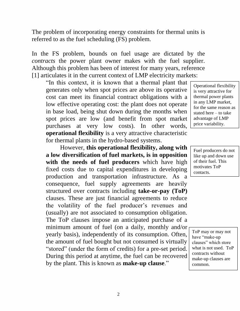
The problem of incorporating energy constraints for thermal units is

referred to as the fuel scheduling (FS) problem.

In the FS problem, bounds on fuel usage are dictated by the

contracts the power plant owner makes with the fuel supplier.

Although this problem has been of interest for many years, reference

[1] articulates it in the current context of LMP electricity markets:

“In this context, it is known that a thermal plant that

generates only when spot prices are above its operative

cost can meet its financial contract obligations with a

low effective operating cost: the plant does not operate

in base load, being shut down during the months when

spot prices are low (and benefit from spot market

purchases at very low costs). In other words,

operational flexibility is a very attractive characteristic

for thermal plants in the hydro-based systems.

However, this operational flexibility, along with

a low diversification of fuel markets, is in opposition

with the needs of fuel producers which have high

fixed costs due to capital expenditures in developing

production and transportation infrastructure. As a

consequence, fuel supply agreements are heavily

structured over contracts including take-or-pay (ToP)

clauses. These are just financial agreements to reduce

the volatility of the fuel producer’s revenues and

(usually) are not associated to consumption obligation.

The ToP clauses impose an anticipated purchase of a

minimum amount of fuel (on a daily, monthly and/or

yearly basis), independently of its consumption. Often,

the amount of fuel bought but not consumed is virtually

“stored” (under the form of credits) for a pre-set period.

During this period at anytime, the fuel can be recovered

by the plant. This is known as make-up clause.”

Operational flexibility

is very attractive for

thermal power plants

in any LMP market,

for the same reason as

stated here – to take

advantage of LMP

price variability.

Fuel producers do not

like up and down use

of their fuel. This

motivates ToP

contacts.

ToP may or may not

have “make-up

clauses” which store

what is not used. ToP

contracts without

make-up clauses are

common.

3

There are main types of fuel for thermal power plants, with % of US

electricity supply:

Coal (51% in 2008, 45% in 2010, 42% in 2011)

Natural gas (17% in 2008, 23% in 2010. 25% in 2011)

Petroleum (less than 1% throughout)

Although petroleum is not used at a significant level to supply

power plants on a percentage basis of national energy (<1%), there

are some areas where it is a bit higher (e.g., in New England, 2008,

oil-fired units comprised 24.9% of total capacity and 2% of energy

production [2]).

It is clear from the above quote that suppliers of these fuels can

operate more efficiently if they can obtain take-or-pay (ToP)

contracts, effectively reducing their uncertainty.

A ToP contract is where the buyer pays for a minimum amount of

fuel whether it is taken or not. The price paid under non-delivery

may be equal to or less than the price paid for delivery.

The ToP contract enables the supplier to plan more precisely in

regards to fuel production.

Most contracts also include a ceiling on how much fuel can be used

in a certain period.

2.0 Minimizing costs for fleet with an energy constrained unit

We first consider that an owner of a fleet of N power plants, none of

which are energy constrained, wants to minimize their costs over a

time period. The plants are base-loaded and so guaranteed to be

running. Notationally, we follow W&W (section 6.2) according to:

Fij(Pij): fuel cost rate for unit i during interval j.

Pij: power output for unit i during interval j.

PRj: total demand in period j.

nj: number of hours in jth

period.

4

We desire to solve the following optimization problem:

N

i

ijRj

N

i

ijij

j

j

j

jjPP

PFn

1

max

11

,...,1 ,0

subject to

)(minmax

(1)

where the objective function is the total cost (not cost rate) over all

periods, and the equality constraint is the requirement that in any

one period, the supply must equal demand. We are not accounting

for generator power production limits at this point.

Now let’s consider if there is one machine (or a group of machines)

for which the owner has engaged in a ToP contract with a ceiling.

Mathematically, the simplest case is when the minimum “take”

equals the ceiling. This means that over the jmax time periods, the

unit must use exactly a particular amount of fuel. Let’s call this

amount of fuel qTOT.

qTOT will have units of RE (“raw energy”) and will be different for

each fuel type:

Coal: RE=tons

Gas: RE=ft3

Oil: RE=bbl (barrel=42 gallons)

Let the unit under the ToP contract be unit T=N+1 (so that we have

N units with unlimited fuel contracts).

Define qTj as the fuel input rate for unit T in the jth

time period.

Whereas units of qTOT are RE, the units of qTj are RE/hr).

Note that qTj is a function of PTj, i.e., qTj=qT(PTj). in RE/hr.

How to get this function qTj=qT(PTj)?

5

Define Kf as the energy content of fuel, in MBTU/RE. Typical

values for Kf are:

Fuel Kf (MBTU/RE)

Coal – anthracite 25.64 MBTU/tons

Coal - bituminous 23.25 MBTU/tons

Coal - lignite 22.72 MBTU/tons

Natural gas 0.001 MBTU/ft3

(standard pressure)

Petroleum 5.88 MBTU/bbl

Another way to think about this is that the below quantities of fuel

provide 1 MBTU:

Fuel 1/Kf (RE/MBTU) Other units

Coal – anthracite 0.039 tons/MBTU 78lbs/MBTU

Coal - bituminous 0.043 tons/MBTU 86lbs/MBTU

Coal - lignite 0.044 tons/MBTU 88lbs/MBTU

Natural gas 980 ft3/MBTU

(standard pressure)

10ft×10ft×10ft/MBTU

Petroleum 0.17 bbl/MBTU 7 gallons/MBTU

Recall that H, the heat rate, is MBTU/MWhr and that it is a function

of the power generation level, i.e., H=H(PT). Then the fuel per

MWhr will be H(PT)/Kf, and multiplying this by the power

generation level PT results in the fuel rate, i.e.,

Tjf

TjTjTTj P

K

PHPqq

)()(

(2)

Back to our “simplest case” where the minimum “take” equals the

ceiling, the summation of fuel use by unit T over all time intervals

must equal the fuel requirement qTOT, that is

max

1

j

j

TOTTjj qqn (3)

6

Our new problem, then, will be exactly as our old problem as posed

in (1), with three exceptions.

1. Add the constraint (3).

2. Add fuel costs of our energy-constrained unit to the objective

function.

3. Include in the power balance equation generation corresponding

to the energy-constrained unit, for each time period.

Therefore, the problem statement for the constrained energy

problem becomes:

max

maxmax

1

1

max

111

,...,1 ,0

subject to

)()(min

j

j

TOTTjj

N

i

TjijRj

TjTj

j

j

j

N

i

ijij

j

j

j

qqn

jjPPP

PFnPFn

(4)

The above problem statement can be simplified, however, by

recognizing that the energy-constrained unit must utilize exactly

qTOT of fuel, and since the cost of generation is dominated by the

fuel costs, the last term in the objective function will be a constant.

Since constants in the objective function do not affect the decision

to be made (i.e., the solution, as indicated by the decision variables),

then we may just remove that term, resulting in the following

revised problem statement:

max

max

1

1

max

11

,...,1 ,0

subject to

)(min

j

j

TOTTjj

N

i

TjijRj

N

i

ijij

j

j

j

qqn

jjPPP

PFn

(5)

7

Let’s make the following definitions, corresponding to the two

equality constraints of (5):

max

1

1

max

0)()(

,...,1 ,0)(

j

j

TOTTjTjTj

N

i

TjijRjijj

qPqnP

jjPPPP

(6)

Then, the problem statement can be written more concisely as:

0)(

,...,1 ,0)(

subject to

)(min

max

11

max

Tj

ijj

N

i

ijij

j

j

j

P

jjP

PFn

(7)

The Lagrangian becomes:

)()()(

)(

)(

),,,(

maxmax

max

max

max

111

1

1 1

11

Tj

j

j

ijjj

N

i

ijij

j

j

j

j

j

TOTTjTj

j

j

N

i

TjijRjj

N

i

ijij

j

j

j

jTjij

PPPFn

qPqn

PPP

PFn

PP

L

(8)

Now we can write the optimality conditions.

The first optimality condition we will consider is

Since Fij is in $/hr, when multiplied by hr

gives units for the Lagrangian of $. This

means λj must be in $/MW and γ must be

$/(fuel-units), where “fuel-units” are ft3

(for natural gas) or ton (for coal).

8

0)(

)(

max

max

max

1

1 1

11

j

j

TOTTjTjij

j

j

N

i

TjijRjjij

N

i

ijij

j

j

jijij

qPqnP

PPPP

PFnPP

L

(9a)

Performing the differentiation, we obtain

0)(

j

ij

ijijj

ij P

PFn

P

L (9b)

Now consider the optimality condition

0)(

)(

max

max

max

1

1 1

11

j

j

TOTTjTjTj

j

j

N

i

TjijRjjTj

N

i

ijij

j

j

jTjTj

qPqnP

PPPP

PFnPP

L

(10a)

Performing the differentiation, we obtain

0)(

Tj

TjTjj

Tj P

Pqn

P

L (10a)

Finally, the optimality conditions taking derivatives with respect to

the Lagrange multipliers simply give us those constraints back

again.

In summary, the optimality conditions result in the following

equations:

9

NiP

PFn

P

NiP

PFn

P

jij

ijij

ij

i

ii

i

,...,1 ,0)(

:j Interval Time

,...,1 ,0)(

:1 Interval Time

max

max

max

max

max

1max

11

111

1

L

L

(11)

0)(

:j Interval Time

0)(

:1 Interval Time

max

max

maxmax

max j

j

jjj

max

1

111

1

T

TT

T

T

TT

T

P

Pqn

P

P

Pqn

P

L

L

(12)

N

i

TiR

N

i

TiR

PPP

PPP

1

jjjj

max

1

1111

0:j Interval Time

0:1 Interval Time

maxmaxmax

max

L

L

(13)

max

1

0)(j

j

TOTTjTj qPqn

L (14)

We will next consider two different ways of how to solve these

equations.

3.0 Fuel scheduling solution by gamma search

The approach here will use an inner and an outer search mechanism.

The inner search mechanism will be a standard lambda

iteration for each time period to provide us with all generation

levels for each time period. This search will be conditioned on

an assumption regarding constrained fuel, represented by a

Notice that if γ

is specified, then

the equations of

(11), (12), and

(13) from each

time period are

independent and

each time period

can be solved by

lambda-search.

10

particular value of gamma (γ). Each complete solution of the

inner search will result in a total fuel usage corresponding to

the chosen value of gamma.

The outer search mechanism will be a search on gamma to find

the certain value which results in the fuel usage being just

equal to the desired value qTOT.

This approach is illustrated in Fig. 6.3 of W&W. We will show it,

but first we need to recall how to perform the lambda-search....

Implementation of the inner search mechanism requires expressing

the power output for each machine in each time interval as a

function of lambda for that time interval. From (11), we can write

for time interval k:

NiP

PFn

Pk

ik

ikikk

ik

,...,1 ,0)(

:k Interval Time

L (15)

If we assume Fik(Pik) is quadratic, that is

Ni PcPba)(PF ikiikiiikik ,...,1 2 (16)

then

Ni PcbP

)(PFikii

ik

ikik ,...,1 2

(17)

Substitution of (17) into (15) results in

NiPcbnP

kikiikik

,...,1 ,02

L (18)

Solving (18) for Pik results in

Ninc

bnP

ki

ikkik

,...,1 2

-

(18)

This will give us the generation levels for all of the non-energy-

constrained units but not for the energy-constrained unit.

To obtain the generation level for the energy-constrained unit, we

apply (12) to time interval k.

0)(

Tk

TkTkk

Tk P

Pqn

P

L (19)

11

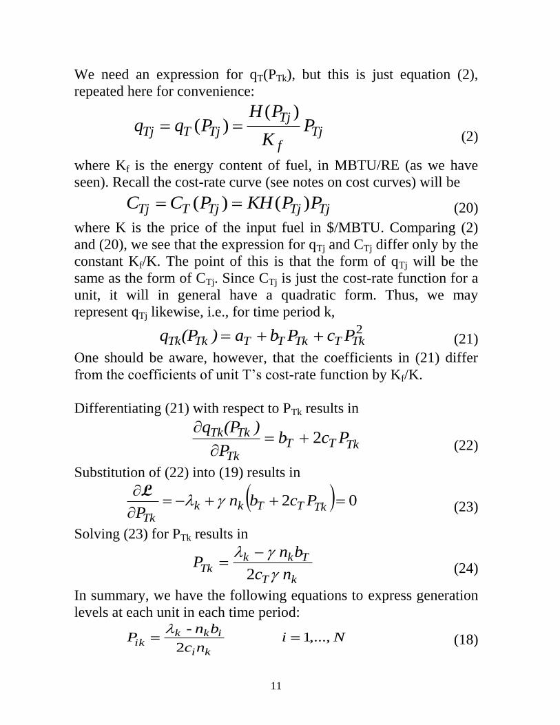
We need an expression for qT(PTk), but this is just equation (2),

repeated here for convenience:

Tjf

TjTjTTj P

K

PHPqq

)()(

(2)

where Kf is the energy content of fuel, in MBTU/RE (as we have

seen). Recall the cost-rate curve (see notes on cost curves) will be

TjTjTjTTj PPKHPCC )()( (20)

where K is the price of the input fuel in $/MBTU. Comparing (2)

and (20), we see that the expression for qTj and CTj differ only by the

constant Kf/K. The point of this is that the form of qTj will be the

same as the form of CTj. Since CTj is just the cost-rate function for a

unit, it will in general have a quadratic form. Thus, we may

represent qTj likewise, i.e., for time period k,

2TkTTkTTTkTk PcPba)(Pq (21)

One should be aware, however, that the coefficients in (21) differ

from the coefficients of unit T’s cost-rate function by Kf/K.

Differentiating (21) with respect to PTk results in

TkTTTk

TkTk PcbP

)(Pq2

(22)

Substitution of (22) into (19) results in

02

TkTTkk

Tk

PcbnP

L

(23)

Solving (23) for PTk results in

kT

TkkTk nc

bnP

2

(24)

In summary, we have the following equations to express generation

levels at each unit in each time period:

Ninc

bnP

ki

ikkik ,...,1

2

-

(18)

12

kT

TkkTk nc

bnP

2

(24)

This will allow us to perform lambda iteration. Note (24) is a

function of gamma.

One thing remains, however. It will be useful to know how to update

lambda following each iteration.

To obtain a lambda update formula, first recall the stopping criterion

for lambda iteration is whether the generation meets the load. This is

expressed by equation (13), which, for interval k, is

N

i

TiR PPP1

kkkk

0

L (25)

Solving for PRk, we obtain

N

i

TiR PPP1

kkk (26)

Now substitute (18) and (24) into (26) to obtain

kT

TkkN

i ki

ikkR

nc

bn

nc

bnP

2

2

-

1

k

(27)

Then we can differentiate (27) with respect to λk to obtain

kT

N

i kik

R

ncnc

P

2

1

2

1

1

k

(28)

We may approximate (28) as

kT

N

i kik

R

ncnc

P

2

1

2

1

1

k

(29)

Solving (29) for ∆ λk, we obtain

kT

N

i ki

Rk

ncnc

P

2

1

2

1

1

k

(30)

13

The Lambda iteration method is illustrated in Fig. 1. Observe that

the flow chart of Fig. 1 assumes that gamma is known; also the

stopping criterion is based on the difference between demand & gen:

Tk

N

i

ikRR PPPP 1

kk

Fig. 1

GUESS λk

k=1

Ninc

bnP

ki

ikkik ,...,1

2

-

2

2

TkTTkTTTk

kT

TkkTk

PcPbaq

nc

bnP

Tk

N

i

ikRR PPPP 1

kk

Is |∆PRk|≤δ

?

Is k=jmax

?

Yes

Yes

No

No

kT

N

i ki

Rk

ncnc

P

2

1

2

1

1

k

koldk

newk

k=k+1

STOP

GUESS γ

14

So Fig. 1 illustrates the “inner loop” of the fuel scheduling solution.

What we need to do now is to identify how to adjust gamma. To do

that, let’s begin by recalling where gamma came from.

We recall the Lagrangian, in (8), repeated here for convenience:

)()()(

)(

)(

),,,(

maxmax

max

max

max

111

1

1 1

11

Tj

j

j

ijjj

N

i

ijij

j

j

j

j

j

TOTTjTj

j

j

N

i

TjijRjj

N

i

ijij

j

j

j

jTjij

PPPFn

qPqn

PPP

PFn

PP

L

(8)

Here we see that that γ is the Lagrange multiplier on the fuel

constraint.

To get a little better feel for γ, recall the fuel constraint (3):

max

1

j

j

TOTTjj qqn (3)

Recall (21)

2TkTTkTTTkTk PcPba)(Pq (21)

Substitution of (21) into (3) results in

max

1

2j

j

TjTTjTTjTOT PcPbanq (31)

What we are after here is the dependence of qTOT on γ. To get this,

recall (24):

15

kT

TkkTk nc

bnP

2

(24)

I will not go through the details here, but rather just articulate the

procedure, which is to substitute (24) into (31) and then differentiate

to obtain ∂qTOT/∂γ. Then, making the approximation

TOTTOT qq

we may derive that

max

13

2

2

j

j jT

j

TOT

nc

q

(32)

I will include my hand-written derivation of (32) in the appendix to

these notes.

We make three comments at this point.

1. From (32), we observe that if γ>0, then ∆γ is always opposite

sign to ∆qT. That is,

Increase γ to decrease fuel usage of Unit T.

Decrease γ to increase fuel usage of Unit T.

2. Analysis of units (see Lagrangian) indicates γ is in $/RE (recall

“RE” is “Raw Energy Units.” This indicates that γ is like a fuel

price. This is consistent with comment #1 – thinking of selling

fuel, if we raise the price, the demand decreases and if we lower

the price, the demand increases.

3. We should recognize, however, that γ is not the fuel price. The

fuel price, also with units of $/MBTU, is given by K – see (20).

So what is γ?

16

Thinking in terms of optimization, as a Lagrange multiplier, we

know that γ represents the change in the objective function of

increasing the right-hand-side of the corresponding constraint by 1

unit.

Said in terms of this problem, γ is the additional cost of requiring the

use of one additional RE unit of fuel at unit T during the next jmax

time periods.

An interesting point made (pg. 174) and proved (Appendix of

Chapter 7) is that the additional unit of fuel could be required in any

time interval. Said another way, γ is constant over time.

The chapter 7 appendix also shows, however, that γ will vary in a

particular time period if both the below are true.

The problem includes constraints on how much fuel can be

used in a particular time period (in addition to the total amount

of fuel to be used over all time periods, which is qTOT). This

can happen for coal-fired plants due to the limitations of coal

stored on site.

The constraint for the particular time period is binding.

Using (32), we are now in a position to draw the entire fuel-

scheduling flow chart, as given in Fig. 2a.

17

Fig. 2a

GUESS λk

k=1

Ninc

bnP

ki

ikkik ,...,1

2

-

2

2

TkTTkTTTk

kT

TkkTk

PcPbaq

nc

bnP

Tk

N

i

ikRR PPPP 1

kk

Is |∆PRk|≤δ

?

Is k=jmax?

Yes

Yes

No

No

kT

N

i ki

Rk

ncnc

P

2

1

2

1

1

k

koldk

newk

k=k+1

max

1

j

j

tjjTOTTOT qnqq

max

13

2

2

j

j jT

j

TOT

nc

q

Is |∆qTOT|<ε

? No

STOP

GUESS γ

Yes

18

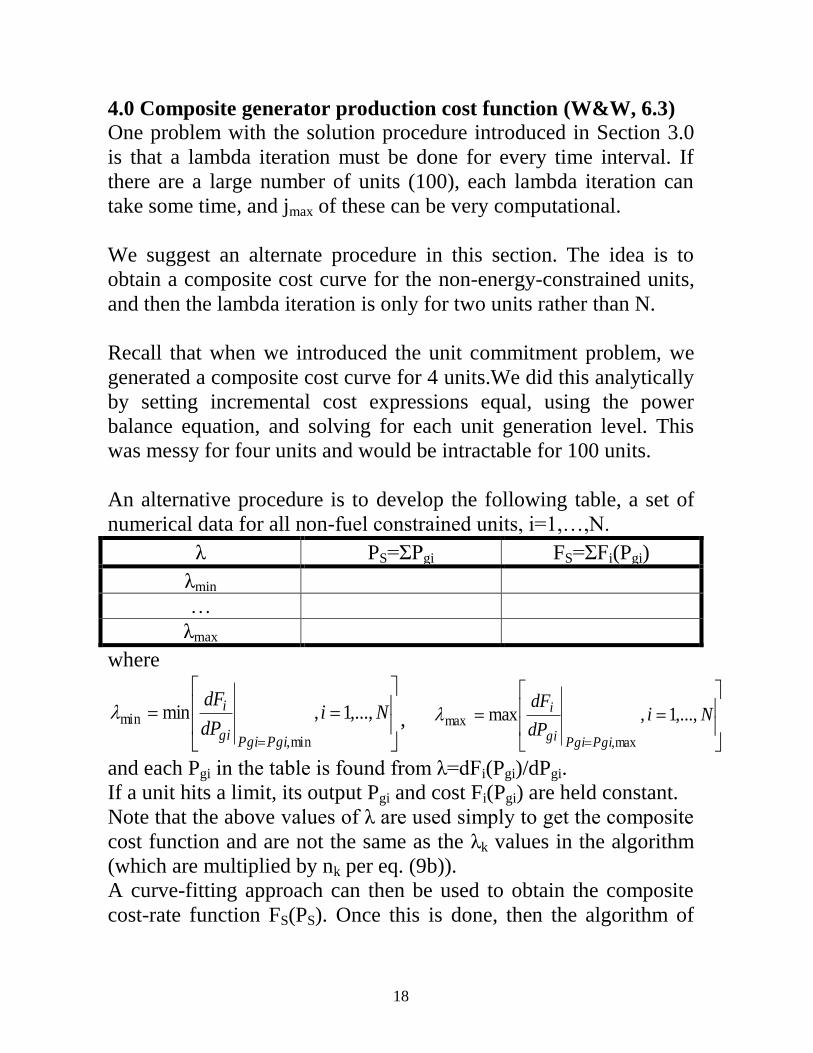
4.0 Composite generator production cost function (W&W, 6.3)

One problem with the solution procedure introduced in Section 3.0

is that a lambda iteration must be done for every time interval. If

there are a large number of units (100), each lambda iteration can

take some time, and jmax of these can be very computational.

We suggest an alternate procedure in this section. The idea is to

obtain a composite cost curve for the non-energy-constrained units,

and then the lambda iteration is only for two units rather than N.

Recall that when we introduced the unit commitment problem, we

generated a composite cost curve for 4 units.We did this analytically

by setting incremental cost expressions equal, using the power

balance equation, and solving for each unit generation level. This

was messy for four units and would be intractable for 100 units.

An alternative procedure is to develop the following table, a set of

numerical data for all non-fuel constrained units, i=1,…,N.

λ PS=ΣPgi FS=ΣFi(Pgi)

λmin

…

λmax

where

NidP

dF

PgiPgigi

i ,...,1,min

min,

min ,

NidP

dF

PgiPgigi

i ,...,1,max

max,

max

and each Pgi in the table is found from λ=dFi(Pgi)/dPgi.

If a unit hits a limit, its output Pgi and cost Fi(Pgi) are held constant.

Note that the above values of λ are used simply to get the composite

cost function and are not the same as the λk values in the algorithm

(which are multiplied by nk per eq. (9b)).

A curve-fitting approach can then be used to obtain the composite

cost-rate function FS(PS). Once this is done, then the algorithm of

19

Fig. 2a is applied, except that there is only 1 non-energy constrained

unit, as shown in Fig. 2b (yellow boxes indicated changes).

GUESS λk

k=1

2

-

kS

SkkSk

nc

bnP

2

2

TkTTkTTTk

kT

TkkTk

PcPbaq

nc

bnP

TkSkRR PPPP kk

Is |∆PRk|≤δ

?

Is k=jmax?

Yes

Yes

No

No

kTkS

R

k

ncnc

P

2

1

2

1

k

koldk

newk

k=k+1

max

1

j

j

tjjTOTTOT qnqq

max

13

2

2

j

j jT

j

TOT

nc

q

Is |∆qTOT|<ε

?

Yes

No

STOP

GUESS γ

20

5.0 Fuel scheduling gradient solution for optimality

Recall the optimality conditions from the Lagrangian. Repeating

(9b),

0)(

j

ij

ijijj

ij P

PFn

P

L (9b)

and (10a),

0)(

Tj

TjTjj

Tj P

Pqn

P

L (10a)

Solving for λj in each of these equations, we obtain

ij

ijijjj

P

PFn

)( (33)

Tj

TjTjj

P

Pqn

)( (34)

Equating (33) and (34), we obtain

ij

ijijj

Tj

TjTjj

P

PFn

P

Pqn

)()( (35)

Solving for γ results in

Tj

TjT

ij

ijij

P

Pq

P

PF

)(

)(

(36)

Observe the numerator and denominator of (36):

Numerator is the Incremental Fuel Cost ($/MW-hr) for non-

fuel constrained units during interval j.

Denominator is Incremental Fuel Rate (RE/MW-hr) for the

constrained unit during interval j.

Our above development shows that, for optimality, this ratio must be

constant for all time intervals j=1,…,jmax. This is consistent with our

previous observation that γ should be constant over time. We can

formulate an algorithm based on this fact, as illustrated in Fig. 3,

adapted from Fig. 6.7a in your text, but we need a feasible schedule.

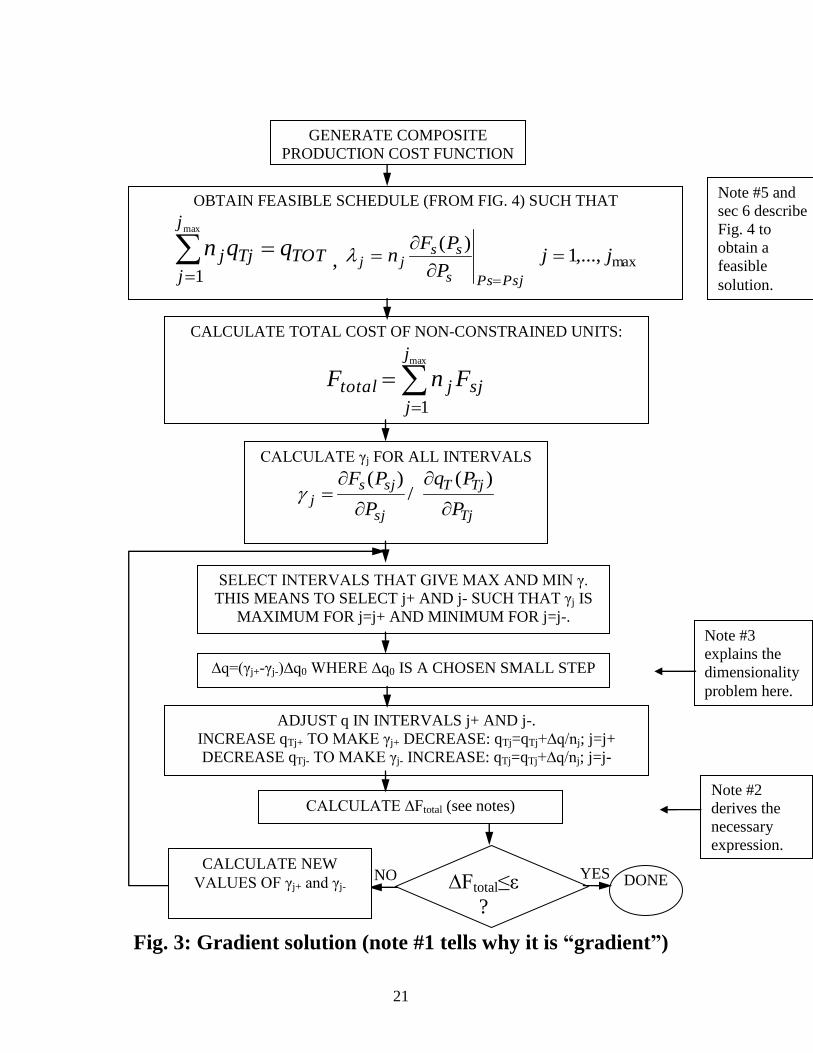
21

Fig. 3: Gradient solution (note #1 tells why it is “gradient”)

GENERATE COMPOSITE

PRODUCTION COST FUNCTION

OBTAIN FEASIBLE SCHEDULE (FROM FIG. 4) SUCH THAT

max

1

j

j

TOTTjj qqn, max,...,1

)(jj

P

PFn

PsjPss

ssjj

CALCULATE TOTAL COST OF NON-CONSTRAINED UNITS:

max

1

j

j

sjjtotal FnF

CALCULATE γj FOR ALL INTERVALS

Tj

TjT

sj

sjsj

P

Pq

P

PF

)( /

)(

SELECT INTERVALS THAT GIVE MAX AND MIN γ.

THIS MEANS TO SELECT j+ AND j- SUCH THAT γj IS

MAXIMUM FOR j=j+ AND MINIMUM FOR j=j-.

∆q=(γj+-γj-)∆q0 WHERE ∆q0 IS A CHOSEN SMALL STEP

ADJUST q IN INTERVALS j+ AND j-.

INCREASE qTj+ TO MAKE γj+ DECREASE: qTj=qTj+∆q/nj; j=j+

DECREASE qTj- TO MAKE γj- INCREASE: qTj=qTj+∆q/nj; j=j-

CALCULATE ∆Ftotal (see notes)

∆Ftotal≤ε

?

DONE CALCULATE NEW

VALUES OF γj+ and γj- YES NO

Note #2

derives the

necessary

expression.

Note #3

explains the

dimensionality

problem here.

Note #5 and

sec 6 describe

Fig. 4 to

obtain a

feasible

solution.

22

We make four comments about the method illustrated in Fig. 3.

1. Your W&W text indicates on pg. 183 that the method “may be

called gradient methods because qTj is treated as a vector and the

γj values indicate the gradient of the objective function with

respect to qTj.” You can observe that this is the case from (36),

using the composite cost-curve, i.e.,

Tj

TjT

sj

sjs

PTj

TjT

Psjs

ss

j

P

Pq

P

PF

P

Pq

P

PF

Tj

)(

)(

)(

)(

(37)

and noting that it must be the case that ∆PSj=-∆PTj, so that

)(

)(

)(

)(

TjT

sjs

sj

TjT

sj

sjs

jPq

PF

P

Pq

P

PF

(38)

showing that γj may be interpreted as a sensitivity of the change

in objective function to a change in the amount of fuel used in

time interval j. If we think of all of qT as a vector, e.g.,

max

1

Tj

T

T

q

q

q

then we may write

max

1

max

1

Tj

s

T

s

sq

jq

F

q

F

FT

as the gradient to Fs.

23

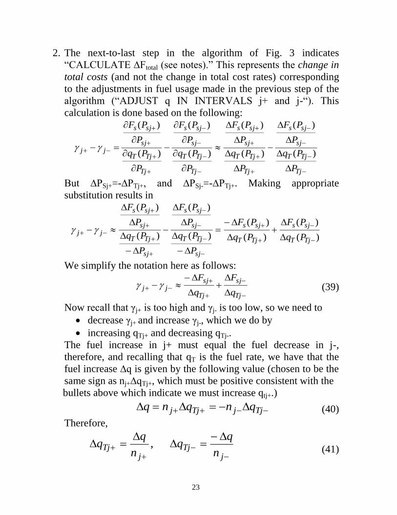
2. The next-to-last step in the algorithm of Fig. 3 indicates

“CALCULATE ∆Ftotal (see notes).” This represents the change in

total costs (and not the change in total cost rates) corresponding

to the adjustments in fuel usage made in the previous step of the

algorithm (“ADJUST q IN INTERVALS j+ and j-“). This

calculation is done based on the following:

Tj

TjT

sj

sjs

Tj

TjT

sj

sjs

Tj

TjT

sj

sjs

Tj

TjT

sj

sjs

jj

P

Pq

P

PF

P

Pq

P

PF

P

Pq

P

PF

P

Pq

P

PF

)(

)(

)(

)(

)(

)(

)(

)(

But ∆PSj+=-∆PTj+, and ∆PSj-=-∆PTj+. Making appropriate

substitution results in

)(

)(

)(

)(

)(

)(

)(

)(

TjT

sjs

TjT

sjs

sj

TjT

sj

sjs

sj

TjT

sj

sjs

jjPq

PF

Pq

PF

P

Pq

P

PF

P

Pq

P

PF

We simplify the notation here as follows:

Tj

sj

Tj

sjjj

q

F

q

F (39)

Now recall that γj+ is too high and γj- is too low, so we need to

decrease γj+ and increase γj-, which we do by

increasing qTj+ and decreasing qTj-.

The fuel increase in j+ must equal the fuel decrease in j-,

therefore, and recalling that qT is the fuel rate, we have that the

fuel increase ∆q is given by the following value (chosen to be the

same sign as nj+∆qTj+, which must be positive consistent with the

bullets above which indicate we must increase qtj+.)

TjjTjj qnqnq (40)

Therefore,

jTj

jTj

n

qq

n

qq ,

(41)

24

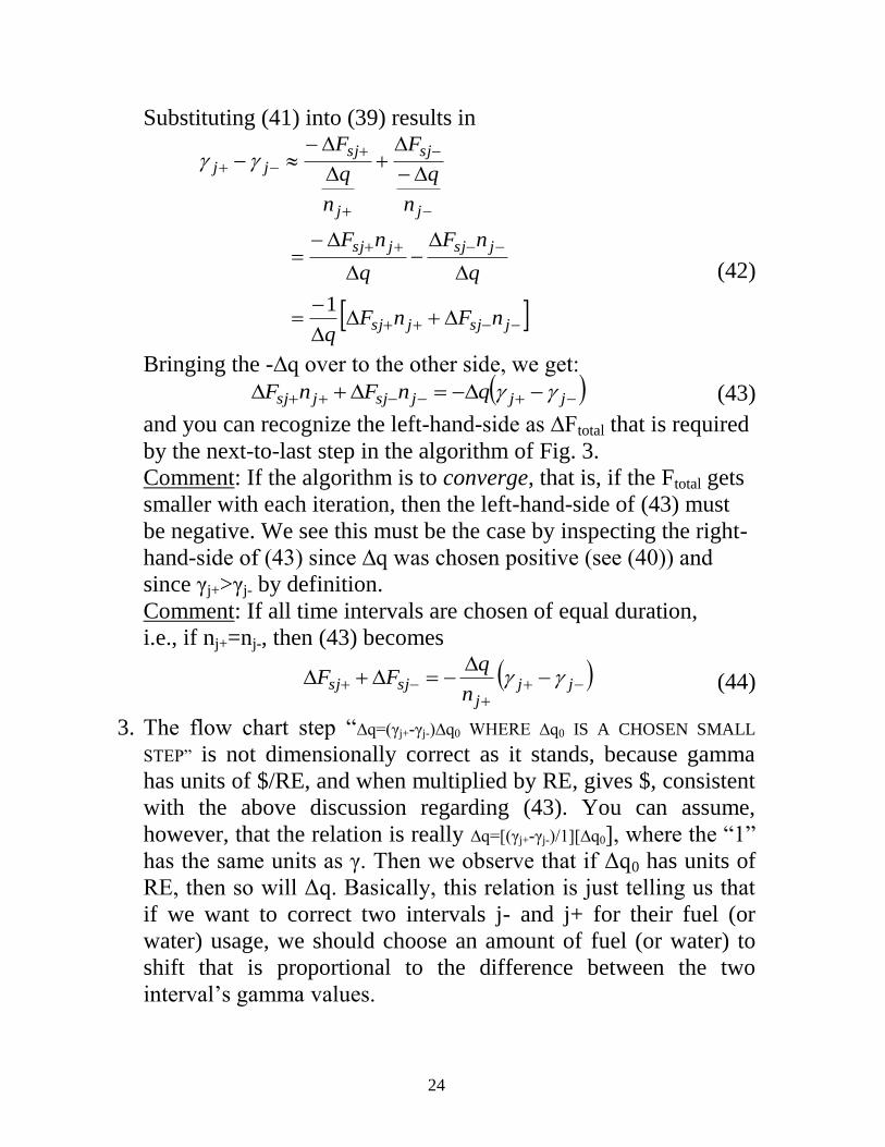
Substituting (41) into (39) results in

jsjjsj

jsjjsj

j

sj

j

sjjj

nFnFq

q

nF

q

nF

n

q

F

n

q

F

1

(42)

Bringing the -∆q over to the other side, we get:

jjjsjjsj qnFnF (43)

and you can recognize the left-hand-side as ∆Ftotal that is required

by the next-to-last step in the algorithm of Fig. 3.

Comment: If the algorithm is to converge, that is, if the Ftotal gets

smaller with each iteration, then the left-hand-side of (43) must

be negative. We see this must be the case by inspecting the right-

hand-side of (43) since ∆q was chosen positive (see (40)) and

since γj+>γj- by definition.

Comment: If all time intervals are chosen of equal duration,

i.e., if nj+=nj-, then (43) becomes

jjj

sjsjn

qFF (44)

3. The flow chart step “∆q=(γj+-γj-)∆q0 WHERE ∆q0 IS A CHOSEN SMALL

STEP” is not dimensionally correct as it stands, because gamma

has units of $/RE, and when multiplied by RE, gives $, consistent

with the above discussion regarding (43). You can assume,

however, that the relation is really ∆q=[(γj+-γj-)/1][∆q0], where the “1”

has the same units as γ. Then we observe that if Δq0 has units of

RE, then so will Δq. Basically, this relation is just telling us that

if we want to correct two intervals j- and j+ for their fuel (or

water) usage, we should choose an amount of fuel (or water) to

shift that is proportional to the difference between the two

interval’s gamma values.

25

4. Observe that stopping criterion is to check to see if Ftotal changes

significantly.

5. The second step in the algorithm of Fig. 3 indicates that it

assumes a feasible (but not necessarily optimal) schedule in that

the fuel use requirement is met and

the generation dispatch of each time interval is “locally

optimal” meaning that it would be the optimal dispatch if

we considered only that time interval.

The problem at hand is: from where do we obtain a feasible

schedule? This is the topic of the next section.

6.0 Fuel scheduling gradient solution for feasibility

This approach is illustrated in Fig. 4.

26

Fig. 4

GENERATE COMPOSITE

PRODUCTION COST FUNCTION

OBTAIN FEASIBLE SCHEDULE IGNORING FUEL CONSTRAINT.

BEST APPROACH IS TO SOLVE ECONOMIC DISPATCH FOR EACH PERIOD.

max,...,1 ,)(

)(

jjP

PFn

P

PFn

Tj

TjTj

sj

sjsjj

CALCULATE TOTAL FUEL USED BY UNIT T

max

1

'j

j

TjjTOT qnq

CALCULATE γj FOR ALL INTERVALS

Tj

TjT

sj

sjsj

P

Pq

P

PF

)( /

)(

DONE (Go to

Fig. 3).

YES

NO

FIND j* WITH MAX γj AND

INCREASE PTj, DECREASE PSj,

TO INCREASE FUEL USE:

qTj=qTj+∆qTj for j=j*

|q’TOT-qTOT|<ε

?

YES

(negative)

NO

(positive)

FIND j* WITH MIN γj AND

DECREASE PTj, INCREASE PSj,

TO DECREASE FUEL USE:

qTj=qTj-∆qTj for j=j*

q’TOT-qTOT <0

?

CALCULATE γj FOR j=j*

Tj

TjT

sj

sjsj

P

Pq

P

PF

)( /

)(

27

Two important observations may be made from Fig. 4:

1. The second block from the top indicates that the algorithm begins

with a feasible schedule for the problem without the fuel

constraint. The best way to obtain this is from an economic

dispatch for each period.

2. The third block obtains the fuel used by the particular chosen

schedule. This is computed by (31), repeated here for

convenience:

max

1

2j

j

TjTTjTTjTOT PcPbanq (31)

Your W&W text provides an example fuel scheduling problem,

which is solved by gamma search (Example 6B, pg. 180-181) and

by the gradient approach (Example 6C, pg. 184-185). Please review

these two examples and know how to work them.

[1] R. Chabar, M. Pereira, S. Granville, L. Barroso, and N. Iliadis, “Optimization of Fuel

Contracts Management and Maintenance Scheduling for Thermal Plants under Price

Uncertainty,” Proc. of the Power Systems Conference and Exposition, Oct. 29-Nov 1,

2006.

[2] H. Chao, “Integration of Natural Gas and Electricity in new England and the rest of

US,” presentation at the 2008 APEX Conference in Sydney, Australia, October 13-14,

2008.