SLAC-PUB-14552 SU-ITP-11/44 NSF-KITP-11-196

FRW solutions and holography from upliftedAdS/CFT

Xi Dong,1 Bart Horn,1 Shunji Matsuura,2,1 Eva Silverstein,1 Gonzalo Torroba1

1Stanford Institute for Theoretical Physics

Department of Physics and SLAC,

Stanford, CA 94305, USA2Kavli Institute for Theoretical Physics

University of California, Santa Barbara, CA

93106, USA

Abstract

Starting from concrete AdS/CFT dual pairs, one can introduce ingredients whichproduce cosmological solutions, including metastable de Sitter and its decay to non-accelerating FRW. We present simple FRW solutions sourced by magnetic flavor branesand analyze correlation functions and particle and brane dynamics. To obtain a holo-graphic description, we exhibit a time-dependent warped metric on the solution andinterpret the resulting redshifted region as a Lorentzian low energy effective field theoryin one fewer dimension. At finite times, this theory has a finite cutoff, a propagatinglower dimensional graviton and a finite covariant entropy bound, but at late times thelower dimensional Planck mass and entropy go off to infinity in a way that is dominatedby contributions from the low energy effective theory. This opens up the possibility ofa precise dual at late times. We reproduce the time-dependent growth of the numberof degrees of freedom in the system via a count of available microscopic states in thecorresponding magnetic brane construction.ar

Xiv

:110

8.57

32v1

[he

p-th

] 2

9 A

ug 2

011

Contents

1 Introduction: keeping it real 1

2 FRW solution sourced by magnetic flavor branes 4

2.1 Magnetic flavor branes . . . . . . . . . . . . . . . . . . . . . . . . . . . . . . 4

2.2 Solution and warping . . . . . . . . . . . . . . . . . . . . . . . . . . . . . . . 6

2.3 Planck mass in d− 1 dimensions and its decoupling at late times . . . . . . . 11

2.4 Covariant entropy bound . . . . . . . . . . . . . . . . . . . . . . . . . . . . . 13

2.5 Basic relations among parameters . . . . . . . . . . . . . . . . . . . . . . . . 14

3 Dynamics of particles and branes 15

4 Degrees of freedom in FRW holography 18

4.1 A microscopic count of degrees of freedom in FRW holography . . . . . . . . 19

4.2 Deriving Ndof from the quasilocal stress tensor . . . . . . . . . . . . . . . . . 23

4.2.1 Quasilocal stress tensor . . . . . . . . . . . . . . . . . . . . . . . . . . 23

4.2.2 Ndof in AdS/CFT and dS/dS . . . . . . . . . . . . . . . . . . . . . . 24

4.2.3 Ndof in the FRW dual . . . . . . . . . . . . . . . . . . . . . . . . . . 26

5 Correlation functions 27

5.1 Massive Green’s functions . . . . . . . . . . . . . . . . . . . . . . . . . . . . 27

5.2 Massless Green’s functions . . . . . . . . . . . . . . . . . . . . . . . . . . . . 30

6 Future directions: Magnetic flavors and time-dependent QFT 32

A Correlation functions in general CdL geometry 34

A.1 Euclidean prescription . . . . . . . . . . . . . . . . . . . . . . . . . . . . . . 34

A.2 Lorentzian prescription . . . . . . . . . . . . . . . . . . . . . . . . . . . . . . 37

A.3 Our FRW spacetime . . . . . . . . . . . . . . . . . . . . . . . . . . . . . . . 41

A.4 Massive correlation functions . . . . . . . . . . . . . . . . . . . . . . . . . . . 43

Bibliography 44

1 Introduction: keeping it real

At present we lack a complete theoretical framework for cosmology. One approach to thisproblem is to try to organize cosmology holographically, building on the success of theAdS/CFT correspondence. Doing so is not trivial for a number of reasons related to the

1

tendency of cosmological solutions to mix with each other and the absence of a simple timelikeboundary. Dynamical gravity, or an integration over metrics, is part of the putative lower-dimensional dual in various attempts so far to generalize the AdS/CFT correspondence tocosmology and describe a complete set of observables; this includes dS/CFT [1] at least asit is interpreted in [2],1 dS/dS [4] and FRW/CFT [5]. Despite the lower dimensional gravity,the formulation of a significant part of the system in terms of a large matter sector is anontrivial step, one which has recently been put on more solid footing microscopically [6].Nonetheless it is important to understand whether a more precise formulation might exist.

The structure of UV complete cosmological solutions will likely be useful in answeringthis question.2 In this paper, we present and analyze concrete cosmological solutions whichare sourced by a generic ingredient – magnetic flavor branes – used to uplift AdS/CFTsystems [7] to cosmology. With sufficiently many magnetic flavor branes, no nonsingularstatic solutions exist, but time-dependent solutions do exist which are nonsingular at latetimes; these solutions are nonsingular at all times if obtained from a bubble nucleationprocess. (Another interesting class of dynamical F-theory solutions was studied in the earlierwork [8], which emphasized the point that no physical restriction on the number of 7-branesexists once the generic possibility of time dependence is included.) We will introduce aholographic interpretation of this class of solutions, employing the following basic strategy.

First, we find a warped metric on our spacetime and interpret the two highly redshiftedregions in terms of a pair of low energy effective theories. This is a generalization of theobservation in [4] that metastable d-dimensional de Sitter spacetime is a warped compactifi-cation with two throats and propagating (d−1)-dimensional gravity.3 This line of reasoningof course goes back to the original arguments [10, 11] that the highly redshifted core regionof a stack of branes should be equivalent to a field theory, since it represents low energydegrees of freedom decoupled from the ambient Planck scale. We verify that particles arestable in the infrared region, though color branes out on their approximate Coulomb branchpropagate up the throat. We call this phenomenon “motion sickness”; as we will discusslater on it is not fatal.

The next step is to compute the (d− 1)-dimensional Newton constant: this reveals thatthe (d − 1)-dimensional graviton decouples at late times, in a way analogous to a Randall-Sundrum theory with the “Planck brane” taken off to infinity. This, and the growth of theentropy at late times [12], is consistent with the possibility of an ultimately precise holo-graphic dual decoupled from gravity. Although gravity decouples in this promising manner,we will see that the way the field theory induces a growing Planck mass is through a rapidly

1For this example, there may at least be a subset of observables which correspond to a precise non-gravitational CFT as described in [2], where the CFT computes the wavefunction of the universe. However,this wavefunction is a functional of the metric which one must ultimately integrate over. See the recent work[3] for more discussion of this question.

2In the somewhat analogous context of black hole physics, study of concrete string theoretic examplesled to microstate counts and ultimately the AdS/CFT correspondence.

3More recently, a description in terms of two CFTs coupled to gravity was motivated in another way by[9].

2

growing number of degrees of freedom, rather than via a growing cutoff on the effective fieldtheory. That is, the system at late times behaves like a theory which is holographic andnon-gravitational, but with a finite cutoff for the dual theory. Cutoff quantum field theoryis in principle well defined, but many questions remain about its detailed implementation ingauge/gravity duality.4

In fact, we find a nontrivial match between the time-dependent number of degrees offreedom in the (d − 1)-dimensional dual theory, computed using the gravity side in threedifferent ways, with an estimate of the number of available microscopic degrees of freedom onthe magnetic flavor branes responsible for the uplift to cosmology. The states we count aredrawn from the infinite algebras discussed in [14], cut off at finite time by backreaction andtopological consistency criteria. As we will describe below, as currently formulated this countis consistent with basic group-theoretic requirements, but is not fully derived. It is subject totwo assumptions about unknown quantities – the first is a plausible conjecture made but notproved in [14], and the second regards the number of charged matter representations whicharise. With these assumptions, our count consistently reproduces the gravity-side resultin a general class of solutions in different dimensions in a way that appears nontrivial, andgeneralizes the parametric microscopic estimate of the dS entropy of [6] to FRW cosmologies.These results seem rather encouraging, and motivate further study of time-dependent fieldtheories with sufficiently many magnetic flavors to provide candidate duals for cosmologicalsolutions.

Our formulation of the holographic dual as a Lorentzian-signature field theory (or ef-fective field theory) maintains standard reality and unitarity properties; in particular thenumber of degrees of freedom in the matter sector is a positive real number. There areother interesting approaches to de Sitter or FRW holography which define the dual on aspacelike (Euclidean) surface, and it would be interesting to study the relation betweenthese different formulations.5 It may be useful to note, however, that because of the ulti-mate requirement of integrating over metrics, the argument for defining the theory on theboundary of the spacetime does not trivially generalize from AdS to dS or FRW solutions.Microscopically, large-radius de Sitter solutions in string theory do not arise as a simplecontinuation of AdS solutions, which turns the flux imaginary in the Freund-Rubin solu-tion. The physically consistent metastable dS solutions that are known arise instead byuplifting AdS solutions with a more complicated collection of stress-energy sources. As wewill see, defining a Lorentzian-signature dual via our warped metric does not a priori forceus to forego a complete dual description: our warped solution decompactifies at late times,somewhat analogously to Randall-Sundrum with the Planck brane removed to infinity.

Another basic motivation for this work is to further develop our understanding of thestructure of time-dependent and cosmological solutions in string theory. We compute correla-

4There has been interesting recent progress in relating radial slices to RG scale in AdS/CFT [13], butthe detailed dictionary remains to be understood, and is subject to various important subtleties such as thefact that different types of gravity-side particles have different relationships between their energy and theirradial position.

5In particular, an interesting approach to a concrete example of dS/CFT can be found in [15].

3

tion functions of massive and massless particles in our geometry; the latter requires a carefultreatment of pseudotachyon modes [16]. The structure of these correlation functions shouldtell us much more about holography on our solutions, the detailed analysis of which we leavefor future work. One intriguing feature is that the two-point function of Kaluza-Klein modesis a power law, rather than exponential.

This paper is organized as follows: In the next section we present FRW solutions sourcedby magnetic flavor branes uplifting Freund-Rubin compactifications. We exhibit a warpedmetric on the solution, indicating a low energy sector corresponding to an effective fieldtheory. In Section 3, we show that particles remain stably in the throat at late times, andcolor branes move up the throat. This theory is cut off and coupled to gravity at finite times,but the Planck mass and the number of degrees of freedom go off to infinity at late timesin a manner that is dominated by contributions of the warped region, raising the possibilitythat the dual completes to a precise non-gravitational theory in this limit. We compute thenumber of field theoretic degrees of freedom in several macroscopic ways in Sections 2 and4.2, and also present, in Section 4.1, a count of brane degrees of freedom which agrees withthe macroscopic predictions given certain assumptions. In Section 5, we study the two-pointcorrelation functions of scalar fields in our solutions, in the massive and massless cases; afull derivation is relegated to Appendix A. Finally, we conclude in Section 6, and outlinedirections for future study.

2 FRW solution sourced by magnetic flavor branes

We would like to understand whether FRW cosmology in d dimensions, which occurs forexample after decays of metastable de Sitter, admits a (d− 1)-dimensional holographic dualdescription. Our strategy is to look for a warped metric on the FRW solutions derived fromuplifted AdS/CFT solutions in string theory. We then interpret the infrared region of thewarped metric – the region of strong gravitational redshift – in terms of a dual effective fieldtheory (EFT). Finally, we analyze whether the EFT might become a self-contained quantumfield theory (QFT) in the far future, since the entropy bound and the (d − 1)-dimensionalPlanck mass go to infinity in that limit.

2.1 Magnetic flavor branes

The simplest AdSd/CFTd−1 dual pairs arise from Freund-Rubin compactifications on a pos-itively curved Einstein manifold Y stabilized by flux. These can be understood as thenear-horizon backreacted solution obtained from color branes placed at the tip of a cone Cwith base Y .

We will uplift to cosmological solutions by adding heavy branes which reverse the signof the curvature of Y . Consider first the AdS5 × S5 solution of type IIB string theory, withthe S5 viewed as a Hopf fibration over a base CP2 (there are many similar examples withS5 replaced by a more general Einstein space Y ). As discussed in [7], there is a natural

4

ingredient which competes with the internal curvature: (p, q) 7-branes at real codimensiontwo on the CP2, wrapping the Hopf fiber circle and extended along AdS5. Such branes can bedescribed using F-theory [17], which geometrizes the varying axio-dilaton, and one finds that36 7-branes are required to exactly cancel the curvature of the CP2. Similarly, 24 7-branesare required to exactly cancel the curvature of a CP1, which arises as the base of the Hopffibration in examples with a compactification on S3, such as AdS3 × S3 × T 4. In the lattercase, alternatively one can use “stringy cosmic 5-branes”[18, 19], elliptic fibrations with thetorus fiber coming from the T 4. See for instance [6], where SC5-branes together with otheringredients are used to cancel the curvature of CP1.

Let us denote the elliptic fibration over the base B = CPm – the CPm with 7-branes atreal codimension two – by B, and the entire uplifted compactification by Y . Parameterizethe number n of 7-branes or stringy cosmic branes in all cases by defining a quantity

∆n ≡ n− nflat (2.1)

such that ∆n = 0 corresponds to a flat uplifted base B.

In the AdS case ∆n < 0, such configurations including their backreaction on the geometrycan be described relatively simply using F-theory. On the field theory side, these systemshave magnetic flavors, arising in the brane construction from (p, q) strings stretching betweenD3-branes and the (p, q) 7-branes [20, 21].

Bringing 7-branes together in a time-independent manner generically introduces singu-larities. For sufficiently few 7-branes, it is understood how these singularities are resolvedphysically, giving enhanced symmetries and/or light matter fields. In a gauged linear sigmamodel (i.e. toric) description of the geometry of the elliptic fibration, singularities appear asadditional branches in the target space [22]. A criterion for physically resolved singularitiesof these static solutions [7] is that the central charge of the additional branch be less thanthat of the main target space of the sigma model. In this case, one may formulate a braneconstruction with 7-branes intersecting at the tip of a cone, at which the color branes areplaced.

This geometry and the backreacted solutions were described in [23, 7]. Its salient featuresare captured by the five dimensional theory obtained by compactifying on S5 and addingthe potential energy of the 7-branes. The effective potential in 5D Einstein frame is

U ∼M55 (RfR

4)−2/3

(R2f

R4+

∆n

R2+

N2c

R8R2f

)(2.2)

where Rf

√α′ is the size of the fiber circle S1

f , and R√α′ is the size of the uplifted base B.

The first term is from the metric flux of the S1 fiber, and the second is the net contributionof the internal curvature and seven-branes. In this F-theory setting there is generically noglobal mode of gs. There are additional scalar fields from 7-brane moduli, which are relativelyflat as discussed in [7]. A simple case to consider is one in which the dilaton is fixed at anSL(2,Z) invariant point, via the mechanisms discussed in [23]. The third term comes from

5

Nc units of 5-form flux corresponding to the color branes. The middle term will concern usmost in this work; it comes from the 7-brane sources.

The 7-branes wrap AdS5 × S1f times a two-cycle in the base, and in the dimensionally

reduced theory we do not keep track of their positions in the compact directions. As reviewedin [7], the geometrical understanding [17] of 7-branes as an elliptic fibration makes it possibleto calculate their leading contribution to the curvature, and hence to the potential energy(2.2). One can study the geometry by realizing it as the target space of a gauged linear sigmamodel [22]. In this description, the beta function for the size of the negatively curved internalspace has the same scaling but opposite sign as in the case of a CPm, by an amount ∆nthat depends on the number of 7-branes. The deformations of the 7-brane configuration aresuperpotential terms in the sigma model and are intrinsically lighter. We can for conveniencefocus on configurations where the string coupling has been fixed at gs ∼ 1, enforced byappropriate combinations of 7-branes; it is also interesting to consider the orientifold limit[24]. The static solutions with ∆n < 0 are then described by minima of (2.2) [7].

Bringing ∆n ≥ 0 branes together in a static configuration leads to singularities whichviolate the above condition for allowed singularities, with the central charge of the singularbranch being larger than that of the main target space. From the point of view of the de-scription (2.2), ∆n ≥ 0 leads to a decompactification limit. Moreover, in such a configurationthe states that transform under the infinite algebras realized on (p, q) 7-branes [14], whichare broken for separated 7-branes, appear to come down to zero mass. These effects hintthat an infinite set of degrees of freedom may ultimately be involved in formulating physicsin the generic case of ∆n > 0, and we will return to this point after developing a controlledgravitational description of uplifted solutions.

In general, we should allow for time-dependent backreacted solutions [8]. As we will ex-plain shortly, the 7-branes need not come together anywhere at late times, and in appropriateexamples (such as [6]). An initial singularity may be avoided by matching to a Coleman-deLuccia tunneling process in the past (as described in Appendix A), though we will in anycase focus on the late time physics in the present work.

2.2 Solution and warping

Let us now introduce our solutions for ∆n > 0. It is interesting to analyze this class ofsolutions both from a ten-dimensional perspective and using the d-dimensional descriptionobtained by compactification on the uplifted space Y . Below, we will exhibit a precise 10dsolution, but let us begin with the d-dimensional description.

In the case d = 5, we have an effective potential (2.2) for the scalar fields R and Rf .With ∆n > 0, the 7-branes overcompensate the contribution of the curvature to the effectivepotential, so they turn the base CP2 into a net negatively curved space B, whose curvaturescales with R as if it were a hyperbolic space. All terms in the potential (2.2) are positive inthis case, and we look for time-dependent solutions where the radii evolve with time (alongwith the FRW scale factor a(t) in the d-dimensional theory).

6

As we will see momentarily, the d-dimensional FRW equations along with the equationsof motion for the scalar fields R and Rf admit a time-dependent solution where at latetimes R and the scale factor expand with time, and the fiber circle Rf remains constant.The dominant term in the potential energy (2.2) in this solution is the term proportionalto ∆n/R2, since the others decay more quickly at large R and fixed Rf . In particular, the5-form flux corresponding to the color branes is very subdominant at late times. We willmake contact with this in Section 3, when analyzing the dynamics of color branes in oursolutions.

Specifically, we find the scale factor a(t) ∝ t, while R ∝ t3/7 and Rf approaches aconstant. The mass of a KK mode on the uplifted base is

mKK ∼nKKR× M5

(R4Rf )1/3∝ nKK

t(2.3)

where the second factor here is the conversion to Einstein frame. This means that, as in theoriginal examples of AdS/CFT [10], there is no hierarchy between the internal dimensionsand the curvature scale in d dimensions. It is likely possible to use the method developed in[7] to obtain a hierarchy of scales, but as we will see shortly our solution is very simple in10 dimensions.

These scalings can be obtained self-consistently by noting that in this limit the dominantcontribution to the energy is given by the 7-branes and curvature, while the fluxes dilutefaster. The FRW equations become

4a

a= −28

3

R2

R2+

2

9M2

5 (R4Rf )−2/3 ∆n

R2

12a2

a2+ 12

K

a2=

28

3

R2

R2+

2

3M2

5 (R4Rf )−2/3 ∆n

R2. (2.4)

Here K is the spatial curvature of the FRW metric. Looking for a solution of the forma(t) = ct, the first equation gives

R(t) =

(7M5

3√

42

∆n1/2

R1/3f

)3/7

t3/7 . (2.5)

Plugging in the second equation yields K = −1 (i.e. an open FRW solution) and c2 = 7/3with a(t) = ct. Note that there will also be a dynamical equation for Rf (t); however,analyzing this equation of motion shows that it is self-consistently frozen in place in theregime above. This and other features of the solution will be very clear in the 10d solutionwe will present shortly. Numerical studies of the equations of motion for a(t), R(t), andRf (t) show that the solution above is an attractor for a range of initial conditions.

Let us now analyze the 10d solution. So far we have focused on (p, q) 7-branes, butsimilar considerations apply more generally to FRW cosmologies sourced by other branesrealized as elliptic fibrations, such as stringy cosmic 5-branes. More generally, other types of

7

sources may be involved. For example, in decay from the metastable dS3 solution in [6], theuplifting contribution arises in part from stringy cosmic 5-branes but also from other sourcessuch as NS5-branes. In general, it is interesting to consider the FRW phase corresponding tothe leading source at late times. The elliptic fibrations we consider here are natural sourceswhich contribute to the curvature at leading order, and we will continue to focus on this casehere.

We then consider a d-dimensional FRW spacetime and an internal space that can bedescribed as a Hopf fibration over a base CPm. As we argued before, as far as the evolutionof the size R of the base goes, the uplifted base B (the elliptic fibration over CPm) behaves likea hyperbolic space H2m of real dimension 2m. Compactifying on this, we find the followingRicci-flat string-frame metric, which is hence a vacuum solution of Einstein’s equation:

ds2s = −dt2s +

t2sc2dH2

d−1 +t2sc2dB2

2m + dx2f , (2.6)

where c2 = (d+ 2m− 2)/(d− 2), c2 = (d+ 2m− 2)/(2m− 1), and

dH2d−1 = dχ2 + cosh2 χdH2

d−2 (2.7)

is the metric on a noncompact, unit hyperboloid of dimension d−1. dB22m is the metric on our

uplifted, negatively curved compact base space of dimension 2m. Although in this work weare concerned with generic configurations with ∆n > 0 branes uplifting AdS/CFT solutions,the solution above also describes the dynamics of a compactification on S1×H2m/Γ, a circletimes a compact hyperbolic space. In that case, the dilaton is meaningful (as oppposed toin F-theory); nevertheless, since our solution is Ricci-flat in 10d string frame, the dilaton isnot sourced in this solution.

In this solution we only included the effects of the flavor branes. In the ∆n < 0 caseof AdS/CFT, the flux corresponding to color branes plays a leading role in the backreactedsolution. However, in the present case at late times the flux dilutes away and is subdominant,as we emphasized above. Furthermore, since the contribution from the metric flux (first termin (2.2)) can also be neglected and the fiber size becomes constant at late times, we haveapproximated the fiber direction by an S1 factor in the geometry.6 In some cases, there maybe additional transverse dimensions (such as the T 4 in models based on AdS3 × S3 × T 4),which we suppressed in the metric (2.6).

Let us now compactify down to d dimensions. The volume of the compactification man-ifold Y is

Vol(Y ) ∝ RfR2m ∝ t2ms , (2.8)

6Although the metric flux is subdominant in the solution, it does affect the topology; in particular thefiber circle remains contractible. This feature will play a role in our count of brane degrees of freedom inSection 4.1. The nontrivial fibration of the circle is a feature of the AdS/CFT dual pair which we are upliftingto FRW cosmology, so the metric flux may be an important element even though its energetic contributionis subdominant. More generally, it would be interesting to develop a holographic duality for the solutionwithout any metric flux.

8

where we have not kept track of time-independent coefficients and have used R ∼ ts from(2.6). Going to the d-dimensional Einstein frame

g(d)µν,E =

(Vol(Y )M8

10

Md−2d

)2/(d−2)

g(d)µν,s, (2.9)

we get an FRW metric of the form

ds2E = −dt2 + c2t2dH2

d−1 , (2.10)

where

c2 =d+ 2m− 2

d− 2, t ∝ tc

2

s . (2.11)

Cases of particular interest are uplifts of AdS5 × S5, with c2 = 7/3 (d = 5, m = 2) anduplifts of AdS3× S3× T 4, with c2 = 3 (d = 3, m = 1). This reproduces the results obtainedusing the d-dimensional theory: R(t) ∝ t1/c

2, in agreement with (2.5).

Since c > 1, the scale factor is expanding faster than in curvature dominated FRW (a.k.a.flat spacetime in Milne coordinates). In general, ∆n > 0 corresponds to c > 1, and we willfind it very useful to contrast our results for c > 1 with the case of flat space (c = 1).Our holographic interpretation will apply consistently for c > 1, and will not apply to flatspacetime.

We may change variables by setting

t = (η2 − w2)c/2 , χ =1

2log

η + w

η − w, (2.12)

and the metric (2.10) becomes

ds2 = c2(η2 − w2)c−1(dw2 − dη2 + η2dH2

d−2

). (2.13)

This metric exhibits warping for c > 1, which corresponds to ∆n > 0. We want to understandthe spectrum and dynamics of degrees of freedom that are redshifted to low energies.

It is useful to consider a closely related time coordinate tUV = ηc, giving metric

ds2 = c2(t2/cUV − w

2)c−1

dw2 +

(1− w2

t2/cUV

)c−1 (−dt2UV + c2t2UV dH

2d−2

). (2.14)

On the UV slice w = 0, we have tUV = t. In this metric the warp factor

f(w, tUV ) ≡(

1− w2

t2/cUV

)(c−1)/2

(2.15)

and the metric component gww depend only weakly on the coordinate time at late times:∣∣∣∣∂tUVf

∂wf

∣∣∣∣ ∼ ∣∣∣∣∂tUVgww

∂wgww

∣∣∣∣ ∼ t−(1−1/c)UV → 0 as tUV →∞ (2.16)

9

where in the last equivalence we have evaluated a point at constant warp factor, i.e. constantw/t

1/cUV . This is not a covariant quantity, but neither is the redshifted energy and the small

value of the ratio (2.16) may simplify some calculations at late times.

There are other ways of writing the FRW spacetime as a warped product metric: asa simple example, we may pass to the conformal time T = 1

clog(tUV /`) in the (d − 1)-

dimensional theory, where ` is an arbitrary length scale. We can absorb the scale factor ctUV(in d− 1 dimensions) into the warp factor and write the warped metric as

ds2 = c2(`2/ce2T − w2)c−1dw2 + c2`2e2cT

(1− w2

`2/ce2T

)c−1

(−dT 2 + dH2d−2). (2.17)

The dual theory now lives on a static (non-expanding) space R×Hd−2. This is similar to theAdS/CFT correspondence written on global vs. Poincare slicing, or other slicings with anexpanding or static hyperboloid [25]. These various slicings describe a dual theory living ondifferent spacetimes. In our case, a complication is the presence of time-dependent couplingsand (in general) a time-dependent metric for the field theory. Furthermore, since the dualtheory is not conformal, the conformal transformation that removes the factor e2cT alsomodifies the running couplings, as we discuss in Section 2.5. Other, more general slicingsmay lead to even more complicated dual descriptions: for instance, using Gaussian normalcoordinates starting from a central spatial slice (hyperbolic or otherwise) gives different w-dependences in the temporal and spatial warp factors. Although we will stick to the simplerexample given above in this work, it would be interesting to consider the existence of dualtheories for more general slicings.

Again, using the warped metric given above, we wish to determine what light (meaningenergy bulk Planck mass Md) degrees of freedom there are. Given a region of stronggravitational redshift, i.e. a region of light states in our gravity solutions, the system mayhave a right to a field theory description as in the low energy regime of the usual AdS/CFT.

The proper time interval between two events of coordinate interval ∆tUV is

∆T (w, tUV ) = ∆tUV

(1− w2

t2/cUV

)(c−1)/2

. (2.18)

This redshift factor is, of course, 1 for c = 1 (flat spacetime), and for c > 1 it is smallerthan 1. This indicates gravitational redshift for probes of proper energy ∼ 1/∆T (fixed inunits of the d-dimensional Planck mass Md). Energies of such probes are redshifted downby a factor of f(w, tUV ) defined in (2.15). As we mentioned above, this is time-dependentas well as dependent on the “radial” scale w, but its w dependence is stronger (2.16). Slicesof constant w/tUV

1/c are then slices of constant scale. In terms of the coordinates given in(2.12), this corresponds simply to slices of constant χ.

This effect arises in the absence of any flux, suggesting that the flavor branes (or moregenerally the geometry they source) support dynamical degrees of freedom in the EFT re-gion.7

7In some examples of AdS/CFT obtained by color branes probing the tip of a cone, there are closed

10

It is important to note that basic degrees of freedom such as KK modes, oscillating closedstrings, 7-7 strings and junctions, D-branes, and so on do not have fixed masses in units ofMd. Their masses depend on t = (t

2/cUV − w2)c/2, leading to t

2/cUV − w2 dependence in ∆T

in (2.18). This is analogous to radially-dependent masses in AdS/CFT.8 For KK modes onthe uplifted base, KK and winding modes on the fiber, strings, and 7-7 strings/junctions weobtain respectively

mKK ∝1

t, mf ∝ mstr ∝

1

t1−1/c2, m77 ∝

1

t1−2/c2. (2.19)

We will analyze their dynamics in Section 3. For our examples, the specific values for theexponents are, respectively, −1, −4/7, −1/7 for m = 2, d = 5, and −1, −2/3, −1/3 form = 1, d = 3.

2.3 Planck mass in d− 1 dimensions and its decoupling at late times

As in Randall-Sundrum theory (RS) [26], we can compute the (d − 1)-dimensional Newtonconstant GN,d−1 by dimensionally reducing on the w direction. This yields

1

GN,d−1

≡Md−3d−1 ∼Md−2

d

∫ t1/cUV

0

dw√−ggtUV tUV (2.20)

∼Md−2d

∫ t1/cUV

0

dw

(1− w2

t2/cUV

) (d−2)(c−1)2

t1−1/cUV ∼Md−2

d tUV . (2.21)

where by gµν we mean the factors that appear in the d-dimensional metric but not in the(d − 1)-dimensional metric. Thus at finite times, we have a warped compactification withpropagating (d−1)-dimensional gravity as in the dS/dS correspondence [4], but as tUV →∞gravity decouples.

This raises the possibility of a more precise field theory dual in the far future. A simplebut nontrivial test of this possibility is the following. In a general warped compactification[27], a diverging (d− 1)-dimensional Planck mass can arise in (at least) two ways:

(1) A leading contribution may come from the warped throat (the effective field theory), asin RS with a Planck brane moving off to infinity. In this case, as the Planck brane goes off toinfinity the holographic dual becomes a pure QFT decoupled from gravity, i.e. the effectivefield theory completes to a full QFT.

string moduli at the tip, for example ones corresponding to Fayet-Iliopoulos terms. The question was raisedin those examples of whether these modes are dynamical. There, the fact that the cone itself was unwarpedsupports the conclusion that the FI term is a parameter, not a field. In more general cases such as ours,however, the answer may be different.

8For example, in AdS/CFT compactified on a circle, momentum modes on the circle become radially-dependent masses for which the redshift factor precisely cancels out, and there are many other examples onecould consider.

11

(2) Instead, in a more general warped compactification the leading contribution may comefrom the volume of the compactification manifold, with the warped throat subdominant. Inthis case, the effective field theory does not complete to a full QFT which captures the fullsystem.

Let us check which of these possibilities is realized in our system. First, let us elaborateon the behavior (1) above in the case of RS. This consists of an AdS5 spacetime

ds2 =r2

R2AdS

(−dt2 + d~x2

)+R2AdS

r2dr2 (2.22)

up to a finite radial scale rUV . The 4-dimensional Planck mass M4 is given by dimensionallyreducing on the radial direction:

M24 ∼M3

5

∫ rUV

0

dr√−ggtt ∼M3

5

r2UV

RAdS

∼ Ndof,AdSΛ2c,RS (2.23)

In the last relation here, which indicates that the Planck mass is induced by the field theorydegrees of freedom, we used that the central charge of the field theory scales like Ndof,AdS ∼M3

5R3AdS [28] and that the energy scale of the cutoff is Λc,RS = rUV /R

2AdS.

For our purposes, it will be useful to belabor this result in the following way. First, letus break up the calculation (2.23) into two pieces: the integral over r from 0 to ε rUV , andthe rest of the integral from ε rUV to rUV , where ε is a fixed constant between 0 and 1. Thisseparates an IR contribution r < ε rUV (corresponding to energies below ε rUV /R

2AdS) from a

UV contribution for r > ε rUV , using an arbitrary reference scale ε rUV /R2AdS that is fixed in

terms of the UV cutoff as we increase rUV . The ratio of the two contributions is a constantas the Planck brane moves off to infinity. In particular, the infrared region continues tocontribute a leading piece to the 4-dimensional Planck mass.

Let us analyze the same question in our FRW case. First, define a scale M∗ dividing theUV and IR regions of our throat via

M∗MUV

≡ ε ⇒ w∗ = t1/cUV

√1− ε2/(c−1) . (2.24)

In terms of this, we can work out the ratio of UV to IR contributions to the Planck mass(2.21), obtaining

UV

IR=

∫√1−ε2/(c−1)

0dy(1− y2)(d−2)(c−1)/2∫ 1√

1−ε2/(c−1)dy(1− y2)(d−2)(c−1)/2

= constant . (2.25)

Thus our setup behaves similarly to case (1), raising the possibility of a pure field theorydual capturing the FRW physics at late times.

12

2.4 Covariant entropy bound

An important quantity that characterizes a field theory is its number of degrees of freedom.For example, if we cut off a theory with a lattice, we require some number Ndof of degreesof freedom per lattice point to define it. That is, we denote the number of field theoreticdegrees of freedom by Ndof. We would like to understand this quantity in our putativeholographic theory, generalizing the analysis given in [28]. There, an infrared cutoff onthe radial coordinate in AdS was related to a UV cutoff in the corresponding QFT. Evenin ordinary AdS/CFT this UV cutoff is not understood very precisely, however: it is notliterally a lattice cutoff since it does not break the isometries of the space on which the fieldtheory lives, and the UV/IR relation works differently for different types of probes on thegravity side. However, gravitational calculations of the entropy of thermal states and of thecentral charges in the field theory reproduce the behavior expected from an identificationof Ndof with the number of degrees of freedom per lattice point, and we may revert to thatlanguage.

We will compute the time dependence of this quantity in several distinct ways in thepresent work, including a count of available states on the magnetic flavor branes, obtainingthe same answer. On the gravity side, a measure of the number of degrees of freedom is givenby the covariant entropy bound [29] on the entropy passing through an observer’s past lightsheet. As emphasized in [12], for FRW solutions (unlike the metastable de Sitter phase) theentropy bound grows to infinity at late times.

Let us work this out explicitly in our solution. We start by choosing a spherically sym-metric set of coordinates on (2.10)

ds2E = −dt2 + c2t2

(dr2

1 + r2+ r2dΩ2

d−2

). (2.26)

Consider an observer at the origin (r = 0) in our space at time t0. The past light cone ofthis observer is foliated by spheres of size ρ = r(t)ct, where r(t) is determined by∫ r

0

dr√1 + r2

= −∫ t

t0

dt

ct⇒ r(t) =

1

2

[(t0t

)1/c

−(t

t0

)1/c]. (2.27)

For c > 1, the sphere grows to a maximal size ρmax ∝ t0 and then begins to shrink (becauseof the contraction of the FRW universe) as we go back in time.

The conjectured entropy bound [29] is given by the area of this maximal sphere in Planckunits. From this we obtain, substituting the time t0 of the observer by t,

S ∼Md−2d td−2. (2.28)

(For c = 1, the sphere never reaches a maximal size, but instead keeps growing, indicatinga diverging entropy bound even at finite time.) In our case, the entropy going to infinity atlate times also suggests the possibility of a precise dual of our FRW phase when t→∞; thisjibes with the infinite warped throat we develop at late times in our solution.

13

2.5 Basic relations among parameters

We are now in a position to list some basic relations between several quantities in our system:the (d − 1)-dimensional Planck mass, the number of field theoretic degrees of freedom Ndof

in the effective field theory (EFT), and the cutoff Λc of the EFT. These relations will enableus to solve for their dependence on time tUV . We will derive Ndof independently usingthe quasilocal stress tensor below in §4.2, obtaining the same result for its dynamics as ispredicted by the simple considerations of this section.

First, since the (d−1)-dimensional Planck mass is largely induced by the field theory (aswe just found in the previous subsection), we have the relation

Ndof Λd−3c ∼ 1

GN,d−1

≡Md−3d−1 ∼Md−2

d tUV (2.29)

where Λc is the cutoff of our effective field theory.

In our (d − 1)-dimensional theory, we expect a nontrivial quantum energy density. Ifwe assume that this is an order one fraction of the source of Hubble expansion in the dual,we obtain a second relation comes from the Friedmann equation in the (d− 1)-dimensionaltheory:

H2d−1 =

1

t2UV∼ NdofΛ

d−1c GN,d−1. (2.30)

Here Hd−1 = 1/tUV is Hubble in the (d − 1)-dimensional theory obtained by dimensionalreduction on w in (2.14).

Putting these together, we find

Ndof ∼Md−2d td−2

UV , Λc ∼1

tUV. (2.31)

This result is consistent with the entropy discussed in the last subsection if we assume thebasic relation

S ∼ NdofΛd−2c Vold−2 (2.32)

where Vold−2 ∼ td−2UV is the volume of space in the dual theory. The result (2.31) is also

consistent with the result for Ndof below in (4.2).

It is also possible to define the theory on a non-expanding lattice using the coordinatiza-tion (2.17), where the (d−1)-dimensional theory lives on R×Hd−2. In this case a calculationanalogous to (2.21) gives

NdofΛd−3c ∼ 1

GN,d−1

∼Md−2d `e(d−2)cT ∼ Md−2

d td−2UV

`d−3. (2.33)

In this case, the Friedmann equation requires that

0 = H2d−1 = GN,d−1ρ+

1

`2(2.34)

14

where ` is the curvature scale of the hyperbolic spatial slices. One implication of this is thatthe energy density must compensate the time dependence in the Newton constant. If weassume again that the energy density is of order NdofΛ

d−1c , we obtain the relation

GN,d−1NdofΛd−1c ∼ 1

`2(2.35)

In this case, we then get

Ndof ∼Md−2d td−2

UV , Λc ∼ constant. (2.36)

Again, this agrees with the covariant entropy bound and with the independent derivationof Ndof we find below in (4.2). Note that the cutoffs in (2.31) and (2.36) are related by aconformal rescaling: to obtain the effective field theory on R×Hd−2, we have to remove theoverall factor e2cT in (2.17) by a conformal transformation. This should be compared with thecorresponding term in (2.14) where there is no such factor. Since our theory does not have aconformal symmetry, this conformal transformation changes the running coupling constantsand other scale dependent quantities. We can see this explicitly in that the gravitationalcoupling GN,d−1 is different in the two cases.

For both slicings, the final result agrees with the scaling (2.28) from the covariant entropybound, since at late times t ∼ tUV . Thus if we think of the cutoff as a lattice cutoff, thesystem builds up entropy by accumulating degrees of freedom per lattice point, rather than byincreasing the number of lattice points. In Section 4.1 we will provide an independent countof Ndof using the magnetic brane construction, finding that the infinite store of degrees offreedom on our ∆n > 0 set of 7-branes, cut off by backreaction criteria, precisely reproducesthis behavior. As described above, these results are consistent with the possibility of acomplete non-gravitational field theory dual at late times, albeit one with a finite cutoff forthe field theory. The growth of Ndof is consistent with this interpretation: in a field theorywith time-dependent masses and couplings, the number of degrees of freedom below a fixedcutoff scale will generically change with time. In our case, it increases rapidly.

3 Dynamics of particles and branes

So far, we have presented our d-dimensional cosmological solution, exhibited a warped met-ric on it, and derived basic properties of its (d − 1)-dimensional description, a candidateholographic dual. In this section we study the motion of particles and branes in our geom-etry. Their motion in the highly redshifted (infrared) region is related to the long distancedynamics of the putative holographic dual. For simplicity we will consider the d = 5 case;general dimensionalities d can be studied in a similar fashion.

Our goals are twofold. First, we would like to better understand the role of the colorsector in our theory, given that the 5-form flux is subdominant in the solution and warpingarises without it. Secondly, we want to check whether the infrared degrees of freedom inthe highly redshifted (warped) throat are stable. In general, it would be interesting to

15

understand what additional criteria – beyond the presence of strong warping – might needto be satisfied in order to obtain a holographic dual capturing the low energy degrees offreedom (see [30] for some earlier discussion of this question). One natural physical criterionis that the strength and variation of the warp factor be such that light particles remain inthe warped region.9

The results are as follows: color branes (D3-brane domain walls) are not stable in the IRregion of our warped geometry, but particles (massive (2.19) and massless) do remain in theinfrared region. These facts can be seen in a simple way from the original metric (2.6) (theyfollow equivalently from a similar analysis using the warped metric).

In the case d = 5, m = 2, the 10-dimensional string frame metric is (2.6)

ds2 = −dt2s +t2sc2

(dχ2 + cosh2 χdH23 ) +

t2sc2dB2

4 + dx2f , (3.1)

where dH23 is the metric on a unit 3-dimensional hyperbolic space H3 and c2 = 7/3. As

mentioned above, slices of constant scale in our warped metric (2.14) translate into slices ofconstant χ, and the two infrared regions correspond to large |χ|.

The isometries of the 4-dimensional hyperboloid, and the corresponding conserved mo-menta, imply that particles that start moving out in the χ direction continue propagatingto larger |χ| as time goes on. Massless particles head toward null infinity, traveling on nullgeodesics dχ = c dts/ts, so that

χmassless(ts) = c log(ts/t0). (3.2)

Massive particles at a fixed point on H3 are governed by the Born-Infeld action

Smassive = −∫dtsm(ts)

√1− χ2t2s/c

2 (3.3)

where the particle mass m(ts) can depend on time in our system. In particular, the string-frame counterparts of (2.19) are:

mKK,s ∝1

ts, mstr,s ∝ mf,s ∝ 1 , m77,s ∝ ts . (3.4)

The conserved momentum is

p =δLδχ

=m(ts)χt

2s/c

2√1− χ2t2s/c

2. (3.5)

A particle at fixed χ = χ0 (with χ = 0 initially) stays at χ0; a particle moving toward thebottom of either throat continues to do so as ts →∞. We can solve for χ using (3.5), giving

χ =cp

ts√p2 +m(ts)2t2s/c

2. (3.6)

9We thank D. Marolf and J. Polchinski for this suggestion.

16

From this we see that in all cases (3.4), χ→ 0 at late times.

At this point we should note that the two-dimensional slice of the spacetime traced out byt and χ (at a fixed point on the H3) is simply flat space, with metric −dt2 + c2t2dχ2. In thatsubspace alone, the low energy region we are defining is a version of a Rindler horizon. Sincec > 1 the spacetime is not flat overall, and the curvature affects generic particle trajectoriesand quantum mechanical wave packets, but a classical calculation of test particle trajectoriesdoes not sense this effect.

We get the same result, of course, by working directly in the d-dimensional warpedmetric given above. There, to analyze particle dynamics we solve the equations of motionfor a particle with a mass of the form m(η, w) ∼ (η2−w2)κ (with κ given by (2.19) for someof the basic particles in our system). In our solution, this is obtained by varying the action

Smassive = −∫dη m(η, w) c(η2 − w2)(c−1)/2

√1− (dw/dη)2. (3.7)

At late η, this yields a solution of the form

w = c1η +c2

ηb(3.8)

with b = 2κ+ (c− 1). In the examples discussed above (KK modes, closed strings, and 7-7strings) b ≥ −1, with equality occurring for the case of KK modes. Again, this means thatsuch particles stay in the infrared region we just defined if they start out there. Note thatwhen transformed back into regular coordinates t, χ, the subleading piece is important toallow the particles to propagate in time.

A D3-brane, on the other hand, experiences a force pushing it up the warped throat. ItsBorn-Infeld action in 10d string frame is of the form

SD3 ∼ −T3

∫dts

(tsc

)3

cosh3 χ√

1− χ2t2s/c2, (3.9)

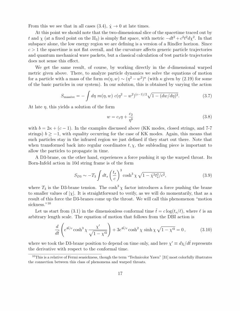
where T3 is the D3-brane tension. The cosh3 χ factor introduces a force pushing the braneto smaller values of |χ|. It is straightforward to verify, as we will do momentarily, that as aresult of this force the D3-branes come up the throat. We will call this phenomenon “motionsickness.”10

Let us start from (3.1) in the dimensionless conformal time t = c log(ts/`), where ` is anarbitrary length scale. The equation of motion that follows from the DBI action is

d

dt

(e4t/c cosh3 χ

χ′√1− χ′2

)+ 3e4t/c cosh2 χ sinhχ

√1− χ′2 = 0 , (3.10)

where we took the D3-brane position to depend on time only, and here χ′ ≡ dχ/dt representsthe derivative with respect to the conformal time.

10This is a relative of Fermi seasickness, though the term “Technicolor Yawn” [31] most colorfully illustratesthe connection between this class of phenomena and warped throats.

17

Deep in the IR of either of our warped throats (e.g. the one with χ 1), (3.10) can bereduced to a first order differential equation for χ′. Integrating this equation reveals thatafter some time (t > 1) the probe D3-brane propagates up the throat and escapes from theIR region, reaching the UV slice χ = 0 within a finite time.11 It is interesting to note thatit takes longer and longer for the branes to escape to this slice at later and later times ts:from (3.9), we have |χ| < c/ts.

Let us remark briefly on the significance of the motion sickness and its time dependence,which should provide useful clues as to the nature of the dual theory. Firstly, it is worthrecalling that motion of color sector eigenvalues up the throat occurs in some familiar ex-amples of AdS/CFT. One example is the case of N = 4 supersymmetric Yang-Mills theoryon a compact negatively curved space [25, 32], where the eigenvalues are subject to a neg-ative quadratic potential. This theory is unitary, because the eigenvalues take forever toget to infinity. The system is properly treated by putting the eigenvalues in a scatteringstate. Another example is Fermi seasickness [33], where finite density effects draw colorbranes up the warped throat. If one cuts off these theories by embedding them in a warpedcompactification then the effect would take a finite time as long as the Planck mass is finite.

A new element in the present case is that the magnetic branes support some warpingby themselves, and the color sector is subdominant in the solution. As we have just seen,particles stay down the warped throat created by the magnetic branes, suggesting that theholographic dual may be built from degrees of freedom living on them.

Altogether, there are two reasons motion sickness does not appear to be fatal in oursystem: (i) the fact that there is an infrared region in the absence of the color D3-branes, and(ii) the fact that even in familiar examples of gauge/gravity duality where the color branesare responsible for all the warping, unitarity is not necessarily sacrificed in the presence of apotential which pushes color branes toward the UV. There are two approaches one can take:(1) eject the offending color branes (treating the color sector as negligible, since the flavorbranes provide warping anyway), or (2) wait it out (keeping the color branes in the game,since the instability takes longer at larger ts).

In particular, in trying to better understand the field theory dual it may remain usefulto think about starting with a color sector in place, since the ejection of the branes takeslonger and longer as ts → ∞. As we will see in the next section, however, the number ofdegrees of freedom is well accounted for by junction states living on the 7-branes themselves.

4 Degrees of freedom in FRW holography

In Section 2 we found that the covariant entropy bound and the number of degrees offreedom per lattice point in the holographic dual grow as td−2. Now we will suggest amicroscopic explanation for this time-dependent growth in terms of states associated to 7-7

11If we set up the system with some 5-form flux (rather than starting with explicit D3-branes), it wouldbe interesting to determine whether, and at what rate, D3-branes are nucleated. The analysis in this sectionshows that once present, color branes do not remain in the warped region for all time.

18

strings and string junctions. These are natural candidates to account for the growing Ndof,because bringing together ∆n > 0 (p, q) 7-branes in a static way leads to infinite dimensionalalgebras [14] that are realized on light states. We make this counting and the assumptionswhich go into it precise in Section 4.1.

In the gravity side, the magnetic flavor branes lead to warping and to an IR region, aswe discussed in the previous sections. In the AdS/CFT correspondence, a warped geometryproduces a nontrivial quasilocal stress tensor that can be used to compute the CFT energymomentum tensor and the central charge. In Section 4.2 we generalize this method tocosmological solutions. This provides an independent calculation of Ndof that agrees withthe microscopic count and with the results in §2.5).

4.1 A microscopic count of degrees of freedom in FRW holography

In this paper we are focusing on quantities we can calculate under control in our gravitysolutions, determining from them various basic features of the putative cutoff field theorydual. This includes several independent computations showing that the number of fieldtheoretic degrees of freedom grows with time as Ndof ∝ td−2

UV . In this section, we will seek amicroscopic accounting of these states. In general, such a count is not guaranteed to work inany simple way; even in systems with a weak coupling limit and a large number of unbrokensupercharges, Ndof generally suffers corrections in going from weak to strong coupling. Forexample, the two are related by a factor of 3/4 in the N = 4 super Yang-Mills theory, andby a more nontrivial interpolation in other examples. Nonetheless, it is interesting to askwhether any natural count of states reproduces the parametric behavior of Ndof in a givenexample.

Rather than going to weak coupling, one may trade fluxes for branes, turning on thecorresponding scalar fields, and study the microstates which are evident in that phase [34].For example, in the N = 4 super Yang-Mills theory if we go out on the Coulomb branchby introducing Nc explicit D3-brane domain walls, the N2

c degrees of freedom of the dualgauge theory become more manifest. In that example, of course, the D3-branes source thewarping, accounting for the low energy sector that indicates the existence of the field theorydual [10].

In our solutions, the 7-branes source warping in themselves. As with flavor branes inAdS/CFT, they do not come together in the backreacted solution (our time dependentsolution), but in the corresponding (singular) static solution they intersect at a point (wherethe color branes are placed in the brane construction). Since they source some warping(like color branes normally do), there is a possibility that there are fundamental degrees offreedom of the dual theory that live on their intersection. Since they dominate at late times(and since the color branes suffer from motion sickness), they may account for the lion’sshare of Ndof. We will explore this possibility in this section, finding rather encouragingresults.

Consider string and string junction states stretching between 7-branes. For the generic

19

case of ∆n > 0, there is an infinite dimensional algebra generated by these junctions [14].12 Ifthe fiber circle were not contractible, they could also a priori carry arbitrarily large momen-tum and winding quantum numbers around that direction. However, they ultimately backreact on the geometry, the fiber circle is ultimately contractible, and Kaluza-Klein momentaare cut off by the giant graviton effect [36], so at any finite time only finitely many states areavailable. In this section, we will estimate the total number of degrees of freedom Ndof atlate times by counting junctions up to a cutoff determined by backreaction and topology. Wewill be concerned with the t-dependence of Ndof, and will not keep track of time-independentfactors.13 The resulting count of brane degrees of freedom will precisely match the behavior

Ndof ∼ td−2UV (4.1)

found above from macroscopic considerations (2.31). As we will describe below, this state-ment is based on two assumptions we will specify.

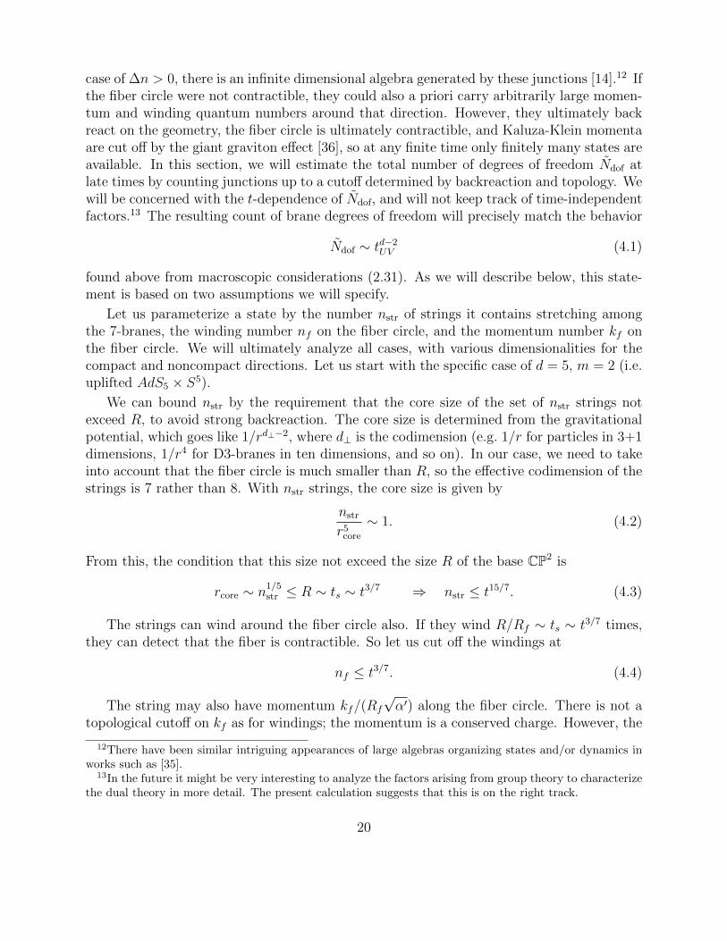
Let us parameterize a state by the number nstr of strings it contains stretching amongthe 7-branes, the winding number nf on the fiber circle, and the momentum number kf onthe fiber circle. We will ultimately analyze all cases, with various dimensionalities for thecompact and noncompact directions. Let us start with the specific case of d = 5, m = 2 (i.e.uplifted AdS5 × S5).

We can bound nstr by the requirement that the core size of the set of nstr strings notexceed R, to avoid strong backreaction. The core size is determined from the gravitationalpotential, which goes like 1/rd⊥−2, where d⊥ is the codimension (e.g. 1/r for particles in 3+1dimensions, 1/r4 for D3-branes in ten dimensions, and so on). In our case, we need to takeinto account that the fiber circle is much smaller than R, so the effective codimension of thestrings is 7 rather than 8. With nstr strings, the core size is given by

nstr

r5core

∼ 1. (4.2)

From this, the condition that this size not exceed the size R of the base CP2 is

rcore ∼ n1/5str ≤ R ∼ ts ∼ t3/7 ⇒ nstr ≤ t15/7. (4.3)

The strings can wind around the fiber circle also. If they wind R/Rf ∼ ts ∼ t3/7 times,they can detect that the fiber is contractible. So let us cut off the windings at

nf ≤ t3/7. (4.4)

The string may also have momentum kf/(Rf

√α′) along the fiber circle. There is not a

topological cutoff on kf as for windings; the momentum is a conserved charge. However, the

12There have been similar intriguing appearances of large algebras organizing states and/or dynamics inworks such as [35].

13In the future it might be very interesting to analyze the factors arising from group theory to characterizethe dual theory in more detail. The present calculation suggests that this is on the right track.

20

tower of momentum modes does not go up forever. Ultimately, it was shown in [36] thatKaluza-Klein momenta are naturally cut off in UV-complete string theoretic examples ofAdS/CFT in exactly the right way to mirror the operator content of the dual field theory. Inthe present case, there is an important crossover at a lower scale. We may view our states asbound states of Kaluza-Klein gravitons and (p, q) string junctions. For sufficiently small kf ,i.e. kf/Rf R, the energy of each stretched string is of order R/

√α′; the gravitons are well

bound to the strings. But when kf crosses over to become much larger than RRf , they arenot strongly bound and the system as a whole behaves like a set of relativistic Kaluza-Kleingravitons of total momentum kf/(Rf

√α′). (Ultimately, as in [36], these gravitons grow into

giants.) Since the gravitons are not strongly bound to the stretched strings (if bound at all),the state may no longer be fundamental. Because of this crossover, we will count kf only upto RRf ∼ t3/7:

kf ≤ t3/7. (4.5)

Finally, we need to determine whether there are additional combinatorial factors whichdepend on nstr arising from the algebra generated by the junctions. To start, let us considerthe configurations classified in [14]. There, one starts from a subset S0 of the (p, q) 7-braneswhich generates a finite Lie algebra G0. One then considers junctions with some prongsending on the S0 branes, transforming under G0 according to their weight vector λ under G0.The rest of the prongs of these junctions form a set of nZ strings with charge (p, q); these endon the remaining 7-branes (or some subset of them) denoted collectively by Z. The works[14] show that a junction with weight λ and asymptotic charge nZ(p, q) satisfies a relation

λ · λ = −J2 + n2Z(f(p, q)− 1). (4.6)

Here J2 ≥ −2 is the self-intersection of the junction, and f(p, q) is a specific function ofthe asymptotic charges (see for example eqn. (2.9) of the second reference in [14]). Sinceλ · λ ≥ 0, f(p, q) ≥ 1 in the generic cases where the full system builds up an infinite algebraGinf . In particular, for f(p, q) > 1 the right hand side of (4.6) can become large and positiveby increasing nZ , and the equation may be satisfied with longer and longer weight vectorsλ in G0. (This is in contrast to the cases with f(p, q) < 1, where at most a finite number ofweights can satisfy (4.6).) It is conjectured in [14] that states with J2 = −2 have the specialfeature that they can be realized by “Jordan Open Strings”, strings that end on two of the7-branes (crossing cuts emanating from the 7-branes in the process). We will count thesestrings.

Given that, next we need to know if there are any multiplicities in the tower of availablestates which grow with nstr at large nstr. As mentioned below (5.52) of the first reference in[14], given a weight vector of length squared λ·λ, there is a degeneracy given by the dimensionof its Weyl orbit. However, this number cannot grow arbitrarily large; it is bounded by thedimension of the Weyl group of G0. In particular, if we consider any individual representationof G0, the number of weight vectors degenerate with the longest weight vector is given bythe Weyl group, and does not grow with n.

There are additional degeneracies in the weight lattice beyond those required by Weyl

21

reflections, but these involve multiple representations. As long as the number of these rep-resentations which arise in our physical system do not grow too fast with nstr, the countwe propose here holds up. It would be interesting to analyze this explicitly for specific Liegroups. This question of which charged matter representations appear in F theory compact-ifications has been studied previously in string theory for phenomenological model building,and similar techniques may be useful in the present case.

Next, let us consider more general configurations which build up ∆n > 0. One wayto think about these is by iterating the procedure just described, considering junctionsstretching between the entire set of 7-branes corresponding to the infinite group Ginf , andan additional (p, q) 7-brane. This works similarly to the above case, except now the Cartanmatrix of the Ginf set of sevenbranes is of indefinite signature. This by itself would allowfor an infinite number of weight vectors of a fixed length squared (schematically of the formλ2

+ − λ2− given the indefinite metric). So in the equation (4.6) there would be an infinite

number of solutions even for finite nZ . However, this infinite number is itself cut off byinsisting that the corresponding junctions be made up of at most of order nstr strings. Thislimits λ+ and λ− above to be at most of order nstr in length, and counting their degeneracyis similar to the above count for finite groups.

Putting this all together, the number of available degrees of freedom is obtained from theproduct of the maximum values of nstr, nf , and kf :

Ndof ∼ (nstrnfkf )max ∼ t15/7+2×3/7 = t3 = td−2 (4.7)

for d = 5.

Next, let us work out Ndof for d = 3, m = 1 (i.e. an FRW uplift of AdS3 × S3 × T 4). Inthis case, the T 4 is of fixed size, independent of t, so (4.2) becomes

nstr

rcore

∼ 1. (4.8)

As a result, (4.3) becomes

r ∼ nstr ≤ R ∼ ts ∼ t1/3 ⇒ nstr ≤ t1/3 (4.9)

Again, the strings can wind around the fiber circle as well. If they wind R/Rf ∼ ts ∼ t1/3

times, they see that the fiber is contractible. So we cut off the windings at

nf ≤ t1/3 (4.10)

and also the momentumkf ≤ t1/3. (4.11)

Altogether we getNdof ∼ (nstrnfkf )max ∼ t = td−2 (4.12)

for d = 3.

22

Having checked it now for two examples, let us finally consider all cases, varying the di-mensionalities of the FRW spacetime and the uplifted internal base space. For d noncompactFRW dimensions and a 2m dimensional uplifted base space, together with one fiber circleand 9− d− 2m toroidal directions, we have

nstr ≤ td+2m−4s , nf ≤ ts, kf ≤ ts (4.13)

where ts is the 10-dimensional string frame time coordinate (2.6). So Ndof goes like td+2m−2s .

Recall that ts goes like t1/c2

in terms of the Einstein frame time coordinate (2.10), andc2 = (d+ 2m− 2)/(d− 2) (2.11). Therefore for the general case, we have

Ndof ∼ td−2 , (4.14)

whose time dependence agrees precisely with the macroscopic calculations of Ndof.

4.2 Deriving Ndof from the quasilocal stress tensor

In the AdS/CFT correspondence, there are several ways to compute the number of degrees offreedom per lattice point of the CFT. For instance, Brown and Henneaux [37] used the con-formal structure of asymptotically AdS3 to identify the central charge, which was rederivedfrom different points of view in [38, 39]. The conformal anomaly can also be computed fromthe variation of the renormalized effective action under a conformal transformation [40, 41].Those analyses, however, depend highly on the conformal symmetry, or on the asymptoticstructure of AdS spacetime. Since our spacetime does not have such a structure, we need toapply other methods.

One possible method is to excite our FRW spacetime and produce a black hole with ahyperbolic horizon in the IR region. The horizon entropy will be identified with that of theeffective field theory, from which we could extract Ndof. This is analogous to the entropycomputation of an AdS black hole in [42].

Another method, which will be applied here, is to compute Brown and York’s quasilo-cal stress tensor [43] and identify it with the expectation value of the stress tensor in theboundary theory. In the context of AdS/CFT, this was used to compute the Casimir energyand Ndof of the boundary theory in [44, 39]. This method can be generalized to the dS/dScorrespondence [4] and to our FRW model. In order to see how it works, let us first reviewthe definition of the quasilocal stress tensor and then use it to calculate Ndof of the dualtheories in both dS/dS and FRW.

4.2.1 Quasilocal stress tensor

Let us consider a spacetime manifold M with a timelike boundary ∂M and space-timemetric gµν . This boundary could be a regularized one at some coordinate cutoff rc. Let nµbe the outward pointing normal vector to ∂M, normalized so that nµn

µ = 1. The inducedmetric on the boundary is given by

γµν = gµν − nµnν , (4.15)

23

where a pullback onto ∂M is understood. The Einstein action including a boundary term is

S =Md−2

d

2

∫Mddx√−g(R− 2Λ)−Md−2

d

∫∂M

dd−1x√−γΘ +Md−2

d Sct[γab], (4.16)

where Θ is the trace of the extrinsic curvature of the boundary

Θµν = −γµρ∇ρnν , (4.17)

Sct is a suitably chosen local functional of the intrinsic geometry γab of the boundary, and a,b are coordinate indices on the boundary. The quasilocal stress tensor [43] is given by

τab ≡ 2√−γ

δS

δγab= Md−2

d

(Θab −Θγab +

2√−γ

δSct

δγab

). (4.18)

The AdS/CFT correspondence relates the expectation value of the stress tensor 〈Tab〉 in thedual field theory to the limit of the quasilocal stress tensor τab as the regularized boundaryat rc is taken to infinity: √

−hhab〈Tbc〉 = limrc→∞

√−γγabτbc, (4.19)

where hab, the background metric on which the dual field theory is defined, is related to theboundary metric γab by a conformal transformation. The counterterms in Sct[γab] are chosenappropriately so as to cancel all divergences when the limit is taken. This has a naturalinterpretation on the dual field theory side: we use local counterterms to obtain a finite,renormalized expectation value of the stress tensor in the field theory.

4.2.2 Ndof in AdS/CFT and dS/dS

Let us calculate the quasilocal stress tensor in AdSd and dSd, both sliced by dSd−1. Themetric is given by

ds2(A)dSd

= R2dw2 + f(w)2ds2dSd−1

, ds2dSd−1

= habdxadxb, (4.20)

where f(w) = sinhw for AdSd and sinw for dSd. Here R is the curvature radius of bothds2

(A)dSdand ds2

dSd−1.

In the AdSd case, the AdS/CFT correspondence says that the bulk is dual to a bound-ary conformal field theory living on dSd−1. In the dSd case, the dS/dS correspondence [4]conjectures that the bulk is dual to two effective field theories living on dSd−1, both of whichare cut off at an energy scale 1/R and coupled to (d − 1)-dimensional gravity and to eachother.

Coming back to our calculation, let us choose a regularized boundary at w = wc. It hasan induced metric γab = f(w)2hab, where hab is the dSd−1 metric on which the field theory isdefined. The extrinsic curvature tensor is

Θab = − 1

Rf(wc)f

′(wc)hab, (4.21)

24

and before adding the counterterms the quasilocal stress tensor is given by

τab =(d− 2)Md−2

d

Rf(wc)f

′(wc)hab =

(d− 2)Md−2

d

R(sinhwc coshwc)hab, for AdSd,

(d− 2)Md−2d

R(sinwc coswc)hab, for dSd.

(4.22)In the AdSd case, the stress tensor is divergent as wc goes to infinity, and the countertermsin Sct renormalize it to

τab ∼Md−2

d

Re−(d−3)wchab (4.23)

for large wc, so that the limit in (4.19) becomes finite and gives 〈Tab〉 ∼ (Md−2d /R)hab.

14

Matching this to the expectation value of the CFT stress tensor on dSd−1 with Ndof degreesof freedom per lattice point

〈Tab〉 ∼Ndof

Rd−1hab, (4.24)

we arrive at the correct number of degrees of freedom per lattice point

Ndof ∼Md−2d Rd−2 (4.25)

in the context of AdS/CFT. In fact we do not have to take wc to infinity to get this parametricresult. We could set wc to be of order 1 and forget about the counterterms (because thereare no divergences to cancel if wc is fixed at order 1, and including the counterterms wouldonly change the numerical coefficients which we are not keeping track of). This gives thesame parametric result for Ndof.

This perspective is important for the dS/dS correspondence, because in this case the wcoordinate is bounded and we cannot take wc to infinity. What we can do is fix wc at order 1,and by the same argument we get Ndof ∼Md−2

d Rd−2. This means that the number of degreesof freedom per lattice point for the dual theory on dSd−1 is parametrically the same as theGibbons-Hawking entropy of dSd. This was confirmed by the concrete brane constructionfor the dS/dS correspondence in [6].

It is interesting to note that the quasilocal stress tensor (4.22) vanishes at wc = π/2 inthe dSd case. This does not contradict our previous result Ndof ∼ Md−2

d Rd−2, because onecan reliably deduce Ndof of the dual field theory only well below its cutoff. The “UV slice”wc = π/2 corresponds exactly to the energy scale where the effective field theory is cut offand coupled to gravity. The vanishing of the quasilocal stress tensor is reminiscent of thegravitational dressing effect discussed in [4]. As we shall see in the next subsection, this alsohappens in our FRW spacetime.

Before going on, we should note that the advantage of being able to take wc to infinityin the AdSd case is that we can calculate the exact Ndof including the numerical coefficients.

14Strictly speaking, the limit is nonzero only for odd d. In even (bulk) dimensions, the limit vanishes andso does the trace anomaly of a CFT in odd (boundary) dimensions. We can still get Ndof by other means.

25

To demonstrate this, let us work for simplicity in d = 3. Only one counterterm is needed inthis case, which is simply a cosmological constant on the boundary: Sct = −(1/R)

∫∂M√−γ.

The quasilocal stress tensor becomes

τab =M3

R(sinhwc coshwc − sinh2wc)hab, (4.26)

which gives 〈Tab〉 = (M3/2R)hab upon taking wc to infinity. The stress tensor from Ndof

free massless scalar fields in dS2 may be calculated in a standard way,15 giving 〈Tab〉 =(Ndof/24πR2)hab. This can also be obtained from the trace anomaly 〈T aa 〉 = (c/24π)R of atwo-dimensional CFT. Matching this result to the quasilocal stress tensor, we arrive at

c ≡ Ndof = 12πM3R, (4.27)

which agrees exactly with [41, 39].

4.2.3 Ndof in the FRW dual

Let us now calculate the quasilocal stress tensor in our FRW spacetime. We start with thewarped metric

ds2d = c2(η2 − w2)c−1(dw2 − dη2 + η2dH2

d−2), (4.28)

and choose the regularized boundary to be a surface of constant α where α is defined byw = αη with 0 < α < 1. This is a hypersurface of constant energy scale relative to the UVcutoff: α ≈ 1 corresponds to the IR, while α 1 corresponds to the UV. The exact valueof α is not essential in our analysis, as long as it is of order 1. This is because our maininterest is the parametric dependence of the quasilocal stress tensor on η (or tUV ), and thisis not affected by the exact location of the hypersurface. One may also consider RG flows inour FRW geometry, as in AdS or dS [46]–[50], and relate Ndof in the IR to its value in theUV. The η-dependence of Ndof is not affected by the energy scale.16

From the coordinate transformation χ = 12

log η+wη−w , a hypersurface of constant α is also a

hypersurface of constant χ = arctanhα, so it is much easier to calculate the quasilocal stresstensor in the usual FRW coordinates

ds2d = −dt2 + c2t2(dχ2 + cosh2 χdH2

d−2). (4.29)

The induced metric on the regularized boundary at χ = χc is given by

γabdxadxb = −dt2 + c2t2 cosh2 χdH2

d−2, (4.30)

15For two-dimensional (and therefore conformally flat) spacetimes one can use Eq. (6.136) of [45]. Notethat their metric convention is the opposite of ours.

16α = 1 is a singular surface and we do not set the hypersurface there. In a broader picture, this singularsurface is replaced by the Coleman–de Luccia instanton and connected to the parent de Sitter space.

26

and the extrinsic curvature can be calculated as

Θtt = 0, Θij = −tanhχcct

γij, (4.31)

where i, j are the coordinate indices on Hd−2. The quasilocal stress tensor is given by

τtt = (d− 2)Md−2

d

ct(tanhχc)γtt, τij = (d− 3)

Md−2d

ct(tanhχc)γij, (4.32)

It is interesting to note that this corresponds to a perfect fluid with equation of state w =(d− 3)/(d− 2). It has vanishing pressure in d = 3.

The next step is to calculate the expectation value of the stress tensor in the dual fieldtheory, which lives on the background metric hab = γab and has Ndof degrees of freedom perlattice point:

〈Tab〉 ∼Ndof

td−1hab. (4.33)

This can be obtained either on dimensional grounds or by using Eq. (6.134) of [45], notingthat γab is conformally flat. Let us set χc to be of order 1 as this is equivalent to setting αto be of order 1. We match 〈Tab〉 to the quasilocal stress tensor (4.32) and obtain

Ndof ∼Md−2d td−2

UV , (4.34)

where we have replaced t with tUV because on a hypersurface of constant α we have t =(1 − α2)c/2tUV ∼ tUV from (2.13). This is in agreement with the microscopic count of thenumber of degrees of freedom.

Just as in the dS/dS correspondence, the quasilocal stress tensor (4.32) vanishes at χc = 0,corresponding to the UV slice w = 0. Again this suggests renormalization from the (d− 1)-dimensional gravitational effects.

5 Correlation functions

In this section we compute two-point functions for massive and massless scalar fields inour solution. These should provide detailed information about the nature of the (d − 1)-dimensional theory. That theory lives on an FRW geometry, has time-dependent and scale-dependent couplings, and is necessarily strongly coupled in order to reproduce a large-radiusgravity solution. We will leave a complete interpretation of our Green’s functions to futurework, but will note some of their interesting features below.

5.1 Massive Green’s functions

In AdS/CFT it is well understood how gravitational scattering amplitudes behave like fieldtheory correlators. For example, massive propagators in the bulk (which are exponentially

27

suppressed in flat space) turn into power-law CFT two-point functions in the dual theorythrough the effects of the warp factor, which is a strong function of the radial distance r.Because of the warp factor, geodesics do not go along fixed-r trajectories; they can takeadvantage of the warp factor and go along a shorter path by moving in the radial direction.This leads to the power law rather than exponential correlators. (A simple discussion of thiscan be found in [28].)

Let us ask the analogous question in our case. Our dual theory is formulated on an FRWspacetime and has a time and scale-dependent coupling corresponding to the radius R of B,which depends on t = (t

2/cUV − w2)c/2. (As noted above (2.16), this quantity depends more

strongly on the radial scale coordinate w than on time tUV .) As we saw in Section 2.5 andSection 4, our theory is cut off at a finite scale, but accumulates additional field theoreticdegrees of freedom as time evolves forward. As a result, the theory is not conformallyinvariant. Nonetheless we will see that there is one sector of massive bulk fields – KK modeson the base B – which have power law correlators.

We will now compute the leading behavior of the 2-point Green’s functions for particlesof mass m(t) ∝ t−α in our geometry. To find the dominant trajectory, we must solve theequations obtained by varying the action

S = −∫dλm(t)

√t2 − c2t2

(χ2 + cosh2 χ ˙χ2 + . . .

), (5.1)

where “dot” represents a derivative with respect to the worldline coordinate λ and dH2d−1 =

dχ2 + cosh2 χ(dχ2 + sinh2 χ dΩ2d−3). We are interested in computing the propagator between

the points (t, χ, χ) and (t, χ, χ + ∆χ). Note that because of the time-dependent mass, thecalculation of the dominant trajectory is not equivalent to a calculation of the geodesicdistance between the two points in our spacetime.

Our result can only depend on time t and on the geodesic distance L between two pointsin Hd−1 because of the isometries of Hd−1. For two points on the same χ-surface, the geodesicdistance L in Hd−1 is given by17

coshL = cosh2 χ cosh ∆χ− sinh2 χ . (5.2)

The central (UV) slice of our warped geometry is at χ = 0. We will be interested bothin Green’s functions formulated deep in the IR at χ 1, and also in Green’s functionsformulated at the UV slice χ = 0.

Since the propagator can only depend on t and on the geodesic distance L, it is actuallyeasier to do the calculation at constant χ and varying χ, and at the end replace this by L.Consider a particle with mass

m(t) =nαtα, (5.3)

17This is the hyperbolic law of cosines, and it can be obtained by analytic continuation from a similarformula on a sphere, or simply from the dot product in the embedding space.

28

where nα is a constant of dimension 1 − α. In the d = 5 case, α = 1, 4/7, and 1/7 for KKmodes, closed strings, and 7-7 strings, respectively. Define the new coordinates

τ =t1−α

1− α, y = (1− α)cχ, (α 6= 1) (5.4)

andτ = log(t/`), y = cχ, (α = 1). (5.5)

Let us first address the KK modes. Setting n1 ≡ nKK we see that the action (5.1) at constantχ reduces to

S = −nKK∫dλ√τ 2 − y2 (α = 1). (5.6)

This is equivalent to the action for a particle with a constant mass in flat spacetime. Theresulting two-point function is e−nKK∆y, exponentially suppressed in ∆y = c∆χ = cL.

However, this is a power law suppression in the geodesic distance ∆X in the (d − 1)-dimensional spacetime −dt2UV + c2t2UV dH

2d−2 on which the d − 1 theory lives. Working at

χ = 0, we have the geodesic distance L = ∆χ according to (5.2). We can see the power lawbehavior by making a coordinate transformation

X = tUV sinh(cχ) , T = tUV cosh(cχ) , (5.7)

where the metric is Minkowskian on the plane spanned by X and T . Taking our two pointsat the same T , i.e. taking χ1 = −χ2 = ∆χ/2, we obtain the geodesic distance (for ∆χ 1)

∆X = 2tUV sinh(c∆χ/2) ≈ tUV ec∆χ/2, (5.8)

and hence our exponential result in ∆χ becomes a power law in ∆X. The Green’s functionis of the form

G(∆x) ∼ e−nKKcL ∼ e−nKKc∆χ ∼ 1

(∆x)2nKK, (5.9)

where ∆x ≡ ∆X/ctUV is the comoving geodesic distance.

This result is quite intriguing, as we obtain power law correlators from a massive KKmode propagator, which is reminiscent of what happens in ordinary AdS/CFT. However,here the mechanism for this involves the time dependence of the mass. The propagator deepin the IR (large χ) and for large ∆χ, has an additional exponential suppression as a functionof χ,

G(χ; ∆x) ∼ e−nKKcL ∼ e−nKKc(2χ+∆χ) ∼ e−2cnKKχ1

(∆x)2nKK, (5.10)

where we used L ≈ 2χ + ∆χ from the large χ, ∆χ limit of (5.2). Recalling that χ =12

log η+wη−w (2.12), we find that the propagator has a power law scaling with w/η. This energy

scaling of the correlator is again characteristic of a CFT, where power-law wavefunctionrenormalization is produced by nontrivial anomalous dimensions. Note that these formulas

29

only apply in the c > 1 case, since for c = 1 the KK masses are constant, and we do not getwarping or this power law behavior.

Next, let us analyze the correlation functions for other massive scalar fields, those forwhich α 6= 1.

S = −nα∫dλ√τ 2 − τ 2y2 (α 6= 1). (5.11)

This action is equivalent to the action for a particle with constant mass nα in the Milneuniverse, and the dominant trajectory is obtained by analytic continuation from flat space:

Scl = 2inατ sinh∆y

2, (5.12)

where the sign can be determined by the −iε prescription implicit in the square root. Ap-proximating the propagator by eiScl and rewriting the action in terms of the geodesic distanceL obtains

G(t;L) ∼ exp

[−2nα

t1−α

1− αsinh

(1− α)cL

2

]. (5.13)

Let us consider the massive fields with α < 1 (closed strings and 7-7 strings) at large∆χ 1, in which case we have L ≈ ∆χ+ 2 log coshχ from (5.2). Note that this expressionis valid for both small and large χ. In terms of the geodesic distance ∆X (5.8) in the (d−1)-dimensional FRW spacetime, the massive Green’s function (5.13) has (for large ∆χ 1) anexponential suppression

G(t; ∆X) ∼ exp

[−nα

t1−α

1− α

(∆X

tUV

)1−α

(coshχ)c(1−α)

]∼ exp

[−nα

(∆X)1−α

1− α

], (5.14)

where we have used tUV = t(coshχ)c from the coordinate transformation (2.12). It is inter-esting to note that the α < 1 Green’s function in this form is independent of χ (althoughthere could be χ-dependent prefactors that we have not kept track of).

These α < 1 fields become parametrically heavy at late times, dying away at long dis-tances as compared to the KK modes with their power law correlators. But they remain partof the theory: as we have seen in Section 4.1, the set of 7-7 strings and junctions which donot strongly backreact on the geometry make a leading contribution to the count of degreesof freedom. This is somewhat reminiscent of off-diagonal matrix elements in the N = 4 SYMtheory out on its Coulomb branch: these are parametrically heavy at large AdS radius ascompared to KK modes, but they cannot be decoupled from the system.

5.2 Massless Green’s functions

One can potentially learn about the field theory dual of a warped gravity solution such asours by studying the massless correlation functions. In this section, we give the correla-tion function of a massless scalar field in our open FRW spacetime, considering the casewhere it comes from a Coleman–de Luccia (CdL) decay [51]. Details on deriving correlation

30

functions in a general d-dimensional CdL geometry, including an explicitly Lorentzian pre-scription without the need to analytically continue the eigenmode expansion, are presentedin Appendix A.

The calculation is of interest more generally, as it requires developing tools to treatpseudotachyon modes [16] which arise from Hubble expansion. These are infrared modeswhich do not oscillate with time, but also do not grow large enough to significantly affectthe background solution. Such modes arise for c > 1, as explained in Section A.3. Ingeneral, these may be treated by putting them in a scattering state and computing correlationfunctions as expectation values in this state. The method we use here involves choosing aparticular state, the Hartle-Hawking vacuum that one obtains from the analytic continuationof the Euclidean CdL geometry.

We consider a minimally coupled massless scalar field φ in our FRW background

ds2d = −dt2 + c2t2dH2

d−1, dH2d−1 = dχ2 + cosh2 χdH2

d−2, (5.15)

where the scale factor a(t) = ct is correct at late times. If this FRW spacetime comes froma CdL decay, the scale factor has to behave like a(t) = t+O(t3) for small t, so that the bigbang t = 0 is just a coordinate singularity.

We are interested in the large t behavior of the equal-time correlator

G(t, χ,∆χ) ≡ 〈φ(t, χ,∆χ)φ(t, χ, 0)〉, (5.16)

where we have put the two points on a hypersurface of constant χ, corresponding to agiven energy scale as discussed in Section 4.2.3. In particular, χ = 0 corresponds to theUV and χ 1 corresponds to the IR of the dual field theory. We use ∆χ to denote thegeodesic separation of the two points in the Hd−2 directions. In Appendix A we organizethe correlation function into an expansion in the large t and large ∆χ limit. The first twoleading terms turn out to be

Gleading(t, χ,∆χ) ∼ ∆χ+ 2 log coshχ, (5.17)

Gsubleading(t, χ,∆χ) ∼ t(d−2)(√

1−1/c2−1)

coshd−2 χe−(d−2)∆χ/2(∆χ+ 2 log coshχ), (5.18)

up to terms that are “pure gauge”.18 The same leading term was obtained in [5].

We rewrite the correlation function in terms of the geodesic distance ∆X in d − 1 di-mensions, which was derived in Section 5.1 to be ∆X ≈ tUV e

c∆χ/2. From the coordinatetransformation (2.12), tUV and t are related by

tUV = t(coshχ)c. (5.19)

18This is because the massless correlator on a compact space such as the Euclidean CdL geometry is onlywell-defined up to arbitrary constants and linear functions of the coordinates. See a more detailed discussionin Section A.1.

31

The leading contribution (5.17) to the correlation function becomes

Gleading(t, χ,∆X) ∼ log∆X

tUV+ c log coshχ = log

∆X

t, (5.20)

where we have used (5.19) in the last equality. We note that this leading term is presentfor both c > 1 and c = 1, and it is independent of the dimension d. This suggests aninterpretation of it as the contribution from the zero mode of φ localized on the UV slice.

The subleading contribution to the correlation function in terms of ∆X is

Gsubleading(t, χ,∆X) ∼ t(d−2)(√

1−1/c2−1)

coshd−2 χ

(tUV∆X

)(d−2)/c(log

∆X

tUV+ c log coshχ

)(5.21)

=t(d−2)(

√1−1/c2−1+1/c)

(∆X)(d−2)/clog

∆X

t, (5.22)

where we have used (5.19) in the second line. This term is dominated by contributions fromthe pseudotachyonic modes, and is present only for c > 1. This is the case we have focusedon in this paper, which has a warped geometry with a consistent description in terms of alow-energy (d− 1)-dimensional dual.

In order to holographically interpret these results for c > 1 in detail, it is necessaryto understand better the behavior of a strongly coupled field theory with time and scaledependent couplings on a (d − 1)-dimensional FRW background. The strong coupling willlimit our ability to compute, but it will be interesting to see if one can determine enoughabout this theory to make detailed comparisons with results such as (5.21). We will leavean in-depth study of this for future work.

6 Future directions: Magnetic flavors and time-dependent QFT

This work raises many interesting questions, which we have only begun to explore. In thissection we describe a few of them.

On the gravity side, we have seen that in the presence of sufficiently many magneticflavor branes to uplift AdS/CFT to cosmology, one has simple time-dependent solutions,whereas the would-be static solutions are singular (as observed before in [8] via anotherclass of time-dependent F-theory solutions). We have exhibited a warped metric on thesesolutions, and have obtained results consistent with the interpretation of the correspondinglow energy region as a (d− 1)-dimensional holographic dual.

It would be very interesting to understand directly from a field-theoretic point of viewwhere the distinction between ∆n < 0 and ∆n ≥ 0 comes from. If there is a condition on thenumber of magnetic flavors (holding fixed other quantities) which corresponds to ∆n < 0,the above results may suggest that time-dependent effects in field theory could change thiscondition. Time dependent couplings affect the scaling dimensions of the correspondingoperators in the effective Lagrangian.19 On sufficiently short timescales, of course, the system

19One interesting new effect of time-dependent couplings in quantum field theory was discussed in [52].

32

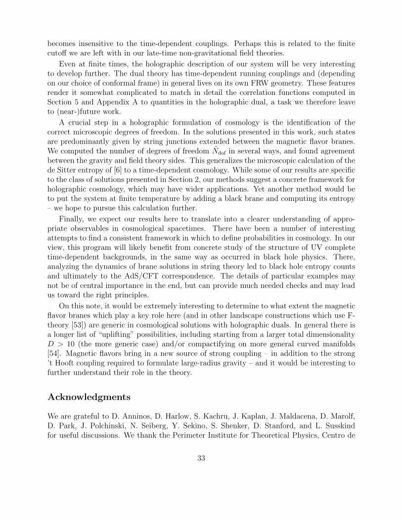
becomes insensitive to the time-dependent couplings. Perhaps this is related to the finitecutoff we are left with in our late-time non-gravitational field theories.

Even at finite times, the holographic description of our system will be very interestingto develop further. The dual theory has time-dependent running couplings and (dependingon our choice of conformal frame) in general lives on its own FRW geometry. These featuresrender it somewhat complicated to match in detail the correlation functions computed inSection 5 and Appendix A to quantities in the holographic dual, a task we therefore leaveto (near-)future work.

A crucial step in a holographic formulation of cosmology is the identification of thecorrect microscopic degrees of freedom. In the solutions presented in this work, such statesare predominantly given by string junctions extended between the magnetic flavor branes.We computed the number of degrees of freedom Ndof in several ways, and found agreementbetween the gravity and field theory sides. This generalizes the microscopic calculation of thede Sitter entropy of [6] to a time-dependent cosmology. While some of our results are specificto the class of solutions presented in Section 2, our methods suggest a concrete framework forholographic cosmology, which may have wider applications. Yet another method would beto put the system at finite temperature by adding a black brane and computing its entropy– we hope to pursue this calculation further.

Finally, we expect our results here to translate into a clearer understanding of appro-priate observables in cosmological spacetimes. There have been a number of interestingattempts to find a consistent framework in which to define probabilities in cosmology. In ourview, this program will likely benefit from concrete study of the structure of UV completetime-dependent backgrounds, in the same way as occurred in black hole physics. There,analyzing the dynamics of brane solutions in string theory led to black hole entropy countsand ultimately to the AdS/CFT correspondence. The details of particular examples maynot be of central importance in the end, but can provide much needed checks and may leadus toward the right principles.

On this note, it would be extremely interesting to determine to what extent the magneticflavor branes which play a key role here (and in other landscape constructions which use F-theory [53]) are generic in cosmological solutions with holographic duals. In general there isa longer list of “uplifting” possibilities, including starting from a larger total dimensionalityD > 10 (the more generic case) and/or compactifying on more general curved manifolds[54]. Magnetic flavors bring in a new source of strong coupling – in addition to the strong’t Hooft coupling required to formulate large-radius gravity – and it would be interesting tofurther understand their role in the theory.

Acknowledgments

We are grateful to D. Anninos, D. Harlow, S. Kachru, J. Kaplan, J. Maldacena, D. Marolf,D. Park, J. Polchinski, N. Seiberg, Y. Sekino, S. Shenker, D. Stanford, and L. Susskindfor useful discussions. We thank the Perimeter Institute for Theoretical Physics, Centro de

33

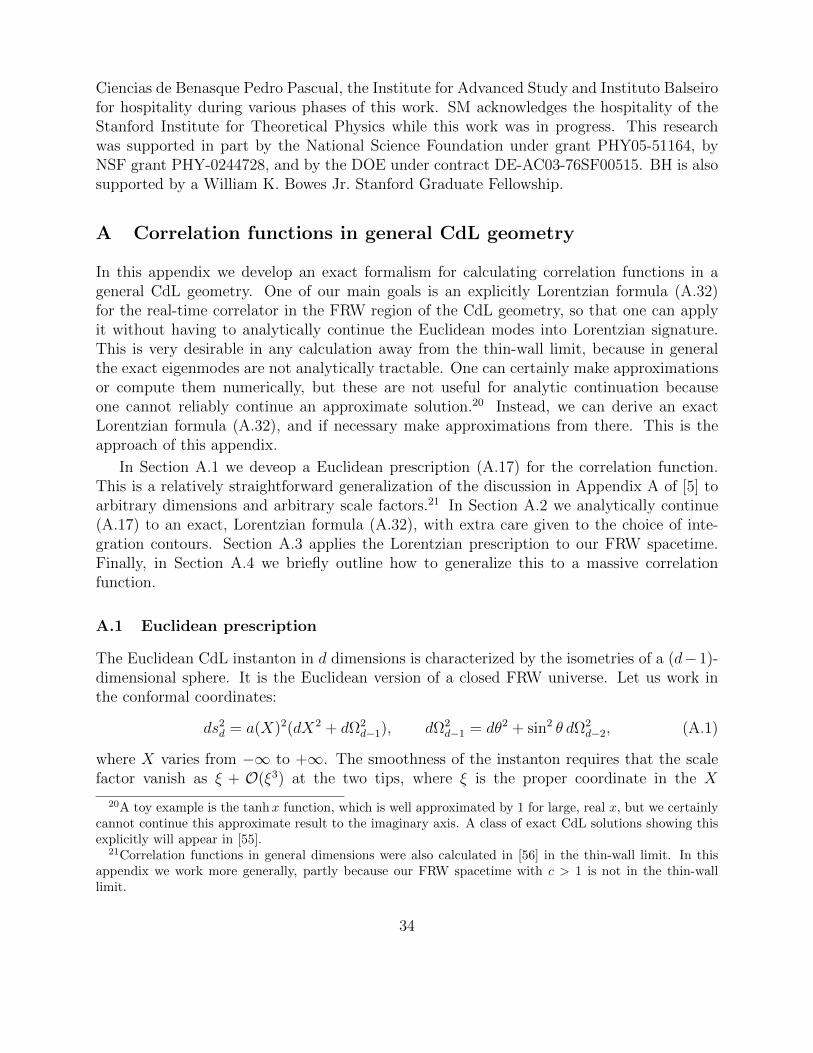
Ciencias de Benasque Pedro Pascual, the Institute for Advanced Study and Instituto Balseirofor hospitality during various phases of this work. SM acknowledges the hospitality of theStanford Institute for Theoretical Physics while this work was in progress. This researchwas supported in part by the National Science Foundation under grant PHY05-51164, byNSF grant PHY-0244728, and by the DOE under contract DE-AC03-76SF00515. BH is alsosupported by a William K. Bowes Jr. Stanford Graduate Fellowship.

A Correlation functions in general CdL geometry

In this appendix we develop an exact formalism for calculating correlation functions in ageneral CdL geometry. One of our main goals is an explicitly Lorentzian formula (A.32)for the real-time correlator in the FRW region of the CdL geometry, so that one can applyit without having to analytically continue the Euclidean modes into Lorentzian signature.This is very desirable in any calculation away from the thin-wall limit, because in generalthe exact eigenmodes are not analytically tractable. One can certainly make approximationsor compute them numerically, but these are not useful for analytic continuation becauseone cannot reliably continue an approximate solution.20 Instead, we can derive an exactLorentzian formula (A.32), and if necessary make approximations from there. This is theapproach of this appendix.

In Section A.1 we deveop a Euclidean prescription (A.17) for the correlation function.This is a relatively straightforward generalization of the discussion in Appendix A of [5] toarbitrary dimensions and arbitrary scale factors.21 In Section A.2 we analytically continue(A.17) to an exact, Lorentzian formula (A.32), with extra care given to the choice of inte-gration contours. Section A.3 applies the Lorentzian prescription to our FRW spacetime.Finally, in Section A.4 we briefly outline how to generalize this to a massive correlationfunction.

A.1 Euclidean prescription

The Euclidean CdL instanton in d dimensions is characterized by the isometries of a (d−1)-dimensional sphere. It is the Euclidean version of a closed FRW universe. Let us work inthe conformal coordinates:

ds2d = a(X)2(dX2 + dΩ2

d−1), dΩ2d−1 = dθ2 + sin2 θ dΩ2

d−2, (A.1)

where X varies from −∞ to +∞. The smoothness of the instanton requires that the scalefactor vanish as ξ + O(ξ3) at the two tips, where ξ is the proper coordinate in the X

20A toy example is the tanhx function, which is well approximated by 1 for large, real x, but we certainlycannot continue this approximate result to the imaginary axis. A class of exact CdL solutions showing thisexplicitly will appear in [55].

21Correlation functions in general dimensions were also calculated in [56] in the thin-wall limit. In thisappendix we work more generally, partly because our FRW spacetime with c > 1 is not in the thin-walllimit.

34

direction. In the conformal coordinates this means a(X) approaches (up to constant factors)eX as X → −∞, and approaches e−X as X → +∞.

We calculate the two-point function of a minimally coupled massless scalar field φ. It isconvenient to consider the rescaled field

φ = a(X)k0φ, where k0 ≡d− 2

2, (A.2)

which has a canonical kinetic term. Note that k0 is the momentum gap for the normalizableeigenmodes of the Laplacian on the unit (d− 1)-dimensional hyperboloid. We let G and Gdenote the correlator of φ and φ respectively. The rotational symmetry of the d− 1 spheremay be used to bring one of the two points to θ = 0, so that the correlator G(X,X ′, θ)depends on no other angular coordinates and satisfies the Laplace equation with a deltafunction source: [

−∂2X −∇2

Sd−1 + U(X)]G(X,X ′, θ) =

δ(X −X ′)δ(θ)Sd−2 sind−2 θ

, (A.3)

where Sn = 2π(n+1)/2/Γ((n + 1)/2) is the volume of the unit n-sphere, and the potentialU(X) is defined as

U(X) =b′′(X)

b(X)= k2

0 −k0Φ′2 + d a(X)2V (Φ)

2(d− 1), where b(X) ≡ a(X)k0 . (A.4)

Here Φ is the scalar field sourcing the metric and has a canonical kinetic term. Its potential22

V (Φ) between the two tunneling points Φ(X = ±∞) is nonnegative for decays from de Sitterto de Sitter or to FRW with a zero cosmological constant (if one assumes the null energycondition), so U(X) is bounded from above by k2

0 and asymptotes to this bound as X → ±∞.

The correlator G(X,X ′, θ) can be obtained as an expansion in the eigenmodes of the“Schrodinger operator” [−∂2

X + U(X)]. The result is

G(X,X ′, θ) =

∫ +∞

−∞

dk

2πuk(X)u∗k(X

′)Gk(θ) +∑κ

uiκ(X)u∗iκ(X′)Giκ(θ), (A.5)

where the first term is an integral over the orthonormal continuum modes satisfying the“Schrodinger equation” [

−∂2X + U(X)

]uk(X) = (k2 + k2

0)uk(X), (A.6)

with the boundary conditions

uk(X)→ eikX +R(k)e−ikX (X → −∞), uk(X)→ T (k)eikX (X → +∞), (A.7)

u−k(X)→ Tr(k)e−ikX (X → −∞), u−k(X)→ e−ikX +Rr(k)eikX (X → +∞), (A.8)

22It is important not to confuse the “Schrodinger potential” U(X) with the potential V (Φ) which sourcesthe geometry. It is also important to distinguish the two scalar fields φ and Φ.

35

where k > 0 is understood. One can show that these coefficients are related by

T (k) = Tr(k),R(k)

R∗r(k)= − T (k)

T ∗r (k), |R(k)|2 + |T (k)|2 = 1. (A.9)

The second term in (A.5) is a discrete sum over the normalized bound states. Theysatisfy the Schrodinger equation (A.6) with k = iκ. There is always at least one bound statefor a compact Euclidean CdL: the zero mode uik0(X) ∝ a(X)k0 . For d ≤ 4 one can showthat this is the only bound state using a technique of supersymmetric quantum mechanics[5]. For d > 4 there may be additional bound states.

The Gk(θ) that appears in (A.5) is the Green’s function on Sd−1 with an appropriatemass: [

−∇2Sd−1 + (k2 + k2

0)]Gk(θ) =

δ(θ)

Sd−2 sind−2 θ. (A.10)

The solution may be written in terms of the hypergeometric function:

Gk(θ) =(2√π)1−d

Γ(d−1

2

) Γ(k0 + ik)Γ(k0 − ik) 2F1

(k0 + ik, k0 − ik,

d− 1

2, cos2 θ

2

), (A.11)

which is a meromorphic function in k. It has simple poles located at

k = ±i(k0 + n), n = 0, 1, 2, · · · (A.12)

due to the Gamma functions in (A.11). In even dimensions the hypergeometric functionsimplifies to an elementary function. For example, in d = 4 (A.11) as a function of complexθ becomes

Gk(θ) =sinh [k(π − θ)]

4π sinh(kπ) sin θ, for 0 < Re(θ) < 2π. (A.13)

The Green’s function Giκ(θ) for the bound states is also given by (A.11). The onlysubtlety appears when we consider the zero energy bound state a(X)k0 with k = ik0, forwhich Gk(θ) hits a pole and diverges. This reflects the fact that the massless correlator ona compact space is ill-defined because we cannot put a single source there without violatingGauss’s law.23 The two-point function for the derivative of a massless field is well-defined andphysical, so one may say that the massless correlator is well-defined up to arbitrary constantand/or linear terms in the coordinates. These terms are called “pure gauge”. Therefore wemay get a finite massless Green’s function by subtracting an infinite constant from Gik0(θ).For example in d = 4 one prescription is

Gik0(θ) = limk→ik0

[Gk(θ)−

1

2π2(k2 + 1)

]+

1

8π2=

cot θ

4π

(1− θ

π

). (A.14)

23The left hand side of (A.10) integrates to zero, but the right hand side does not. This may be solved bysubtracting an inhomogeneous term proportional to the inverse of the volume of the compact space.

36

Before we analytically continue to the Lorentzian signature, let us rewrite the expansion(A.5) in a simpler form. Instead of using uk(X) we might want to write the correlator interms of eigenmodes that have simpler asymptotic behavior as X → −∞, as this is wherewe cross to the FRW region. Let us call this new set of eigenmodes vk(X), defined with theboundary condition vk(X) → eikX as X → −∞ for both positive and negative k. We maywrite them in terms of the old eigenmodes:

vk(X) =u∗−k(X)

T ∗r (k), v−k(X) =

u−k(X)

Tr(k), k > 0. (A.15)

After some algebra, one finds that in terms of the new eigenmodes the continuum contributionin (A.5) becomes

Gc(X,X′, θ) =

∫ +∞

−∞

dk

2π[vk(X)v−k(X

′) +R(k)v−k(X)v−k(X′)]Gk(θ), (A.16)

where the reflection coefficient R(k) is extended from k > 0 to a meromorphic function onthe complex k-plane. For k < 0 one can show R(k) = R∗(−k). One may ask what we haveachieved by rewriting (A.5) as (A.16). It turns out24 that the bound-state contribution in(A.5) can be accounted for, up to pure gauge, by simply deforming the integration contourfor the second term in (A.16). Specifically, the massless correlator (A.5) simplifies to

G(X,X ′, θ) =

∫ +∞

−∞

dk

2πvk(X)v−k(X

′)Gk(θ) +

∫C

dk

2πR(k)v−k(X)v−k(X

′)Gk(θ), (A.17)

where C is a contour that goes from k = −∞ above the double pole k = ik0 to k = +∞, asshown in Figure 1. In the limit X, X ′ → −∞, the second integrand in (A.17) asymptotesto e−ik(X+X′), so we may push the contour C up to Ca, picking up the simple poles atk = i(k0 + n), n = 1, 2, 3, · · · . This is shown in Figure 2a.

Note that R(k) has a simple pole at k = ik0 (corresponding to the zero mode) and azero at k = −ik0, so the second integrand in (A.17) has a double pole at ik0 and is regularat −ik0. It is precisely the residue at the double pole that cancels with the zero energybound state contribution up to pure gauge. For d > 4 there may be additional bound states,corresponding to additional simple poles between k = 0 and k = ik0. There could also beresonance poles, all of which must lie in the lower half plane. As we will see in the next twosubsections, these additional poles need to be taken into account when calculating the exactcorrelation function, but at the order we work, they do not contribute to our final result.

A.2 Lorentzian prescription

Now that we have (A.17) for the massless correlator in the Euclidean CdL geometry, we cananalytically continue it to the FRW geometry

ds2d = a(T )2(−dT 2 + dH2

d−1), dH2d−1 = dr2 + sinh2 r dΩ2

d−2. (A.18)

24This may be shown by expanding the Green’s function in terms of eigenmodes of the Laplacian on Sd−1

(discarding the zero mode). This expansion exactly matches the sum of contributions from the simple polesenclosed by Ca as shown in Figure 2a.

37

k

C

Figure 1: Contour C going from k = −∞ above the double pole k = ik0 to k = +∞.Remember k0 ≡ (d−2)/2. The simple poles above the double pole are located at k = i(k0+n),n = 1, 2, 3, · · · . The locations of the simple poles below the double pole are for illustrationpurposes only and should not be taken too seriously. They depend on the reflection coefficientR(k), and also on whether we are considering the second integrand in (A.17) or in (A.32).The pair of poles away from the imaginary axis are resonance poles.

k

CaHaL k

Cb

HbL

Figure 2: (a) Contour Ca surrounding simple poles at k = i(k0 + n), n = 1, 2, 3, · · · . (b)Coutour Cb surrounding a double pole at k = ik0 and simple poles below ik0. In generalthere could also be resonance poles away from the imaginary axis in the lower half plane, inwhich case the contour Cb needs to enclose them as well.

38

The prescription for the analytic continuation in our conformal coordinates is given by

X → T +iπ

2, θ → ir, a(X)→ ia(T ), vk(X)→ vk(T )e−kπ/2, (A.19)

so that vk(T ) similarly satisfies a “Schrodinger equation”

[−∂2

T + U(T )]vk(T ) = (k2 + k2

0)vk(T ), U(T ) ≡ b(T )

b(T ), b(T ) ≡ a(T )k0 , (A.20)

with the simple boundary condition vk(T )→ eikT as T → −∞.

The Lorentzian correlator G(T, T ′, r) satisfies[−∂2

T +∇2Hd−1

+ U(T )]G(T, T ′, r) =

iδ(T − T ′)δ(r)Sd−2 sinhd−2 r

, (A.21)

and is therefore given (for sufficiently negative T + T ′) by analytically continuing the Eu-clidean correlator (A.17):

G(T, T ′, r) = idG(X → T +iπ

2, X ′ → T ′ +

iπ

2, θ → ir) ≡ G1 + G2 (A.22)

=

∫ +∞

−∞

dk

2πvk(T )v−k(T

′)Gk(r) +

∫Ca

dk

2πR(k)v−k(T )v−k(T

′)Gk(r), (A.23)

where Gk(r) and Gk(r) are defined as

Gk(r) = idGk(θ → ir), Gk(r) = idekπGk(θ → ir) (A.24)

except for the subtlety mentioned below for Gk(r). Let us call the two integrals in (A.23)G1 and G2 respectively. Note that our choice of the contour Ca in G2 is correct only forsufficiently negative25 T + T ′. On the other hand, we are most interested in the masslesscorrelator at late times. If we naıvely increase T + T ′ without deforming the contour Ca, atsome point the integral would diverge. A standard way of solving this problem is to pull thecontour down to C which goes from k = −∞ above the double pole k = ik0 to k = +∞, asshown in Figure 1. Once this is done and the new integral on C agrees with the old one onCa for sufficiently negative T + T ′, we simply use the new integral as the definition for anyvalues of T + T ′. To evaluate this new integral for large T + T ′, one can legally deform thecontour from C to Cb as shown in Figure 2b (at least for some of the terms in the integrand),picking up the double and simple poles below the contour. This last step will be done on acase-by-case basis in the next subsection. Here we first obtain the correct expression for thenew integral on C that is valid for any T and T ′.

It turns out that we cannot naıvely deform the contour from Ca to C in G2. If we dothat, the integral on C would diverge, as we will show shortly. This is different from the

25One can see from (A.29) that “sufficiently negative” here means T + T ′ −r.

39

situation before the analytic continuation, where it does not matter whether we choose C orCa, as long as X+X ′ is sufficiently negative. The main difference is the additional ekπ factorinside Gk(r), which comes from analytically continuing v−k(X)v−k(X

′) to v−k(T )v−k(T′) in

G2.

A hint that something subtle is going on is that we could multiply the integrand of G2 byany number of e2(k−ik0)π factors without changing the integral on Ca. The reason is simplythat the integral on Ca is equal to the sum of residues at the simple poles k = i(k0 + n),n = 1, 2, 3, · · · , and e2(k−ik0)π is simply 1 at all these poles, so none of the residues arechanged. On the other hand, factors such as e2(k−ik0)π definitely matter when the integral isperformed on C. In fact, there is a unique prescription for this factor for which the integralon C is actually convergent. This is the correct prescription, which we will find in exactform below.

Let us use the connection formula for the hypergeometric function

2F1(a, b, c, z) =Γ(c)Γ(b− a)

Γ(b)Γ(c− a)(−z)−a2F1

(a, 1 + a− c, 1 + a− b, 1

z

)+

Γ(c)Γ(a− b)Γ(a)Γ(c− b)

(−z)−b2F1

(b, 1 + b− c, 1 + b− a, 1

z

)(A.25)

to decompose the Gk(r) into two terms:

Gk(r) = idekπ(2√π)1−d

Γ(d−1

2

) Γ(k0 + ik)Γ(k0 − ik) 2F1

(k0 + ik, k0 − ik,

d− 1

2, cosh2 r

2

)(A.26)

= − 1

4πd/2(4z)k0

[e2kπ(4z)−ikΓ(k0 + ik)Γ(−ik) 2F1

(k0 + ik,

1

2+ ik, 1 + 2ik,

1

z

)+(4z)ikΓ(k0 − ik)Γ(ik) 2F1

(k0 − ik,

1

2− ik, 1− 2ik,

1

z

)],

(A.27)

where z is defined as cosh2(r/2). For d = 4 this decomposition looks very simple:

Gk(r) =ekπ sinh [k(π − ir)]4πi sinh(kπ) sinh r

=e2kπ−ikr − eikr

8πi sinh(kπ) sinh r. (A.28)

In general dimensions this decomposition may look complicated, but each term has a simpleasymptotic behavior at large r. Specifically as r →∞, z goes to er/4, both hypergeometricfunctions in (A.27) goes to 1, and we have

Gk(r) ≈ −1

4πd/2ek0r[e2kπe−ikrΓ(k0 + ik)Γ(−ik) + eikrΓ(k0 − ik)Γ(ik)

]. (A.29)

As k → ±∞ along the real axis, the absolute value of the products of Gamma functionsin (A.29) becomes

|Γ(k0 + ik)Γ(−ik)| = |Γ(k0 − ik)Γ(ik)| ≈ 2π|k|d−42 e−|k|π. (A.30)

40

Clearly the first term in (A.29) diverges as k → +∞, while the second term goes to zero ask → ±∞. As we argued earlier, we treat this divergence by multiplying the first term by afactor of e−2(k−ik0)π = (−1)de−2kπ, changing the exact form (A.27) of Gk(r) into

Gk(r) = − 1

4πd/2(4z)k0

[(−1)d(4z)−ikΓ(k0 + ik)Γ(−ik) 2F1

(k0 + ik,

1

2+ ik, 1 + 2ik,

1

z

)+(4z)ikΓ(k0 − ik)Γ(ik) 2F1

(k0 − ik,

1

2− ik, 1− 2ik,

1

z

)], (A.31)

where again z = cosh2(r/2). This does not change the integral on Ca, but enables us tolegally deform the contour from Ca to C for sufficiently negative T + T ′. In terms of thisimproved Gk(r) the Lorentzian correlator is

G(T, T ′, r) = G1 + G2 =

∫ +∞

−∞

dk

2πvk(T )v−k(T

′)Gk(r) +

∫C

dk

2πR(k)v−k(T )v−k(T

′)Gk(r),

(A.32)which looks the same as (A.23) except for the contour C. This is our final, exact expressionfor the massless correlator in any open FRW spacetime resulting from a CdL decay, validfor any T , T ′, and r. Here Gk(r) is given by (A.24) as

Gk(r) = id(2√π)1−d

Γ(d−1

2

) Γ(k0 + ik)Γ(k0 − ik) 2F1

(k0 + ik, k0 − ik,

d− 1

2, cosh2 r

2

). (A.33)

Before concluding this section, let us comment on the structure of (A.32). In order tocalculate the Lorentzian correlator, we only need the eigenmodes vk(T ) and the reflectioncoefficient R(k). For vk(T ) we solve the “Lorentzian Schrodinger equation” (A.20) withthe boundary condition vk(T ) → eikT as T → −∞. For R(k) we in principle need tosolve the “Euclidean Schrodinger equation” (A.6). We cannot in general hope to calculatethe complete Lorentzian correlator by knowing only a(T ) but not a(X) (or vice versa); anexample is provided by the thin-wall limit discussed in [5], where the Lorentzian scale factora(T ) = eT is exactly the same as that of flat space in Milne coordinates, but the masslesscorrelator still has a nontrivial term due to the specific vacuum chosen by the CdL geometry.From the perspective of (A.32), the choice of vacuum is encoded in the reflection coefficientR(k) which must in general be calculated from the Euclidean scale factor a(X). UsuallyR(k) is not analytically tractable away from the thin-wall limit, but fortunately all we needto know in order to calculate the leading behavior of G2 is the fact that R(k) always has asimple pole at k = ik0, and all other poles lie below it.

A.3 Our FRW spacetime

Let us now apply (A.32) to our FRW model

ds2d = −dt2 + a(t)2dH2

d−1, (A.34)

41

where the scale factor a(t) asymptotes to ct at late times. Near the big bang singularityt = 0 the scale factor a(t) = t+O(t3) as required by the smoothness of the CdL instanton.Going to the conformal coordinates T =

∫dt/a(t), the scale factor a(T ) approaches (up

to constant factors) eT as T → −∞, and approaches ecT as T → +∞. Therefore the“Schrodinger potential” U(T ) asymptotes to k2

0 as T → −∞ and c2k20 as T → +∞. This

means that the eigenmodes vk(T ) have the following asymptotic behavior

vk(T )→ eikT (T → −∞), (A.35)

vk(T )→ αkeiT√k2−(c2−1)k20 + βke

−iT√k2−(c2−1)k20 (T → +∞), (A.36)

where αk and βk are analogous to reflection and transmission coefficients. For k > k0

√c2 − 1

the eigenmodes are oscillatory at large T ; for smaller k they are exponentially decaying orgrowing. These are pseudotachyonic modes.

The exact eigenmodes vk(T ) are difficult to solve analytically except for perhaps un-realistically simple U(T ) such as a step potential. Fortunately, we are most interested inthe equal-time massless correlator at large T and large r, for which both vk(T ) and Gk(r)simplify. Specifically in the large T limit v−k(T )v−k(T ) in G2 becomes

v−k(T )2 ≈ α2−ke

−2iT√k2−(c2−1)k20 + β2

−ke2iT√k2−(c2−1)k20 + 2α−kβ−k ≡ v− + v+ + v0, (A.37)

where we have changed the sign of the exponent in v−k(T ) because we choose the squareroot to have a branch cut between k = ±k0

√c2 − 1. In the large r limit (A.31) simplifies to

Gk(r) ≈ −1

4πd/2ek0r[(−1)de−ikrΓ(k0 + ik)Γ(−ik) + eikrΓ(k0 − ik)Γ(ik)

]≡ G− + G+.

(A.38)Therefore the integrand of G2 in (A.32) can be decomposed into six terms:

G2(T, T, r) ≈∫C

dk

2πR(k)(v− + v+ + v0)(G− + G+), (A.39)

where for large |k| we have v± ∼ e±i2kT and G± ∼ e±ikr/ sinh(kπ) up to powers of k.

In the large T , large fixed r limit that we are interested in (i.e. T r 1) we maydeform the contour from C to Ca for the three terms v+(G− + G+) + v0G+, and deform thecontour to Cb for the other three: v−(G− + G+) + v0G−. If we are interested in the large r,large fixed T limit (i.e. r T 1) instead, we simply switch the contours for v+G− andv−G+. In both cases (or more generally, in any large T , r limit), the leading behavior of G2

can be shown to come from the residue of the v−G− term at the double pole k = ik0. Thiscan be evaluated up to numerical factors:

G2(T, T, r) ∼ e2ck0T (2T + r), G2(T, T, r) =G2(T, T, r)

a(T )k0a(T )k0∼ 2T + r, (A.40)

where G2 is the corresponding piece of the original correlator for φ. The first term 2T is apure gauge because it is linear in the coordinates. The second term r is not, because it isactually the geodesic distance on Hd−1 between the two points of the correlation function.

42

To study the holographic dual of our FRW model, we rewrite the metric in hyperbolicslicing

ds2d = −dt2 + a(t)2(dχ2 + cosh2 χdH2

d−2), dH2d−2 = dχ2 + sinh2 χ dΩ2

d−3. (A.41)

Let us put both points of the correlator on a hypersurface of constant χ, with a separationof ∆χ in the χ direction. Their geodesic distance on Hd−1 is therefore

r = arccosh(cosh ∆χ cosh2 χ− sinh2 χ) ≈ ∆χ+ 2 log coshχ, (A.42)

where the approximation holds for large ∆χ and any χ. For large χ the second term on theright hand side of (A.42) simply becomes 2χ, but let us not commit ourselves to that limit.In terms of χ and ∆χ the leading behavior of G2 from (A.40) becomes

G2(t, χ,∆χ) ∼ ∆χ+ 2 log coshχ. (A.43)

This term is present for both c > 1 and c = 1, and it is independent of the dimension d.This suggests an interpretation as the contribution from the zero mode of φ localized on theUV slice.

The leading behavior of the other term in the correlator, namely G1, is dominated bythe contributions of the pseudotachyonic modes. The most pseudotachyonic mode is the onewith k = 0, given by

v0(T ) ∼ ek0T√c2−1. (A.44)

In the large r limit G0(r) as defined in (A.33) goes like re−k0r, so the first term in thecorrelator (A.32) becomes

G1(T, T, r) ∼ re2k0T√c2−1−k0r, G1(T, T, r) ∼ re2k0T (

√c2−1−c)−k0r, (A.45)

which we rewrite in terms of t, χ, and ∆χ as

G1(t, χ,∆χ) ∼ t(d−2)(√

1−1/c2−1)

coshd−2 χe−(d−2)∆χ/2(∆χ+ 2 log coshχ). (A.46)

This term is present only for c > 1, in which case there is a warped geometry with a consistentdescription in terms of a low-energy (d− 1)-dimensional dual.

A.4 Massive correlation functions

We have hitherto focused on massless correlation functions, but it is rather straightforwardto generalize it to massive correlation functions, as we outline below. This provides analternative way of calculating the massive Green’s functions for the KK modes, closed strings,and 7-7 strings in Section 5.1.

Let us consider a scalar field φ with mass m(t) which we allow to be time-dependent. Wecan use the same techniques developed in Sections A.1 and A.2 to calculate its correlation

43

function. The only difference is that we need to add a corresponding mass term a(X)2m(X)2

to the “Schrodinger potential” U(X), and similarly add −a(T )2m(T )2 to U(T ). This makesthe potential U(X) shallower, and the bound states either have larger eigenvalues (for smallmasses) or simply disappear (for large masses). This means that the reflection coefficientR(k) no longer has a pole at k = ik0. The pole is moved down to between k = ik0 and k = 0 ifthere is still a bound state. Therefore, the formulae for both the Euclidean correlator (A.17)and the Lorentzian correlator (A.32) are fully correct, as long as we define the contour C togo from k = −∞ to k = +∞, in a way that goes just below k = ik0 but always above anypossible poles corresponding to bound states.

The pseudotachyonic modes disappear for sufficiently large masses due to the additionalterm −a(T )2m(T )2 in the “Schrodinger potential” U(T ). One can show that in this case theleading term in the correlation function agrees with the estimates in Section 5.1.

Bibliography

[1] A. Strominger, “The dS / CFT correspondence,” JHEP 0110, 034 (2001).[hep-th/0106113]. E. Witten, “Quantum gravity in de Sitter space,” [hep-th/0106109].

[2] J. M. Maldacena, “Non-Gaussian features of primordial fluctuations in single fieldinflationary models,” JHEP 0305, 013 (2003). [astro-ph/0210603].

[3] D. Anninos, G. S. Ng, A. Strominger, “Future Boundary Conditions in De SitterSpace,” [arXiv:1106.1175 [hep-th]].

[4] M. Alishahiha, A. Karch, E. Silverstein, D. Tong, “The dS/dS correspondence,” AIPConf. Proc. 743, 393-409 (2005). [hep-th/0407125];

M. Alishahiha, A. Karch, E. Silverstein, “Hologravity,” JHEP 0506, 028 (2005).[hep-th/0504056].

[5] B. Freivogel, Y. Sekino, L. Susskind, C. -P. Yeh, “A Holographic framework for eternalinflation,” Phys. Rev. D74, 086003 (2006). [hep-th/0606204].

R. Bousso, B. Freivogel, Y. Sekino, S. Shenker, L. Susskind, I-S. Yang, C. -P. Yeh,“Future foam: Nontrivial topology from bubble collisions in eternal inflation,” Phys.Rev. D78, 063538 (2008). [arXiv:0807.1947 [hep-th]].

[6] X. Dong, B. Horn, E. Silverstein, G. Torroba, “Micromanaging de Sitter holography,”Class. Quant. Grav. 27, 245020 (2010). [arXiv:1005.5403 [hep-th]].

[7] J. Polchinski, E. Silverstein, “Dual Purpose Landscaping Tools: Small ExtraDimensions in AdS/CFT,” [arXiv:0908.0756 [hep-th]].

[8] M. Kleban, M. Redi, “Expanding F-Theory,” JHEP 0709, 038 (2007).[arXiv:0705.2020 [hep-th]].

44

[9] D. Harlow, D. Stanford, “Operator Dictionaries and Wave Functions in AdS/CFT anddS/CFT,” [arXiv:1104.2621 [hep-th]].

[10] J. M. Maldacena, “The Large N limit of superconformal field theories andsupergravity,” Adv. Theor. Math. Phys. 2, 231-252 (1998). [hep-th/9711200].

[11] S. S. Gubser, I. R. Klebanov, A. M. Polyakov, “Gauge theory correlators fromnoncritical string theory,” Phys. Lett. B428, 105-114 (1998). [hep-th/9802109];

E. Witten, “Anti-de Sitter space and holography,” Adv. Theor. Math. Phys. 2,253-291 (1998). [hep-th/9802150];

A. W. Peet, J. Polchinski, “UV / IR relations in AdS dynamics,” Phys. Rev. D59,065011 (1999). [hep-th/9809022].

[12] D. Harlow, L. Susskind, “Crunches, Hats, and a Conjecture,” [arXiv:1012.5302[hep-th]].

[13] I. Heemskerk, J. Polchinski, “Holographic and Wilsonian Renormalization Groups,”JHEP 1106, 031 (2011). [arXiv:1010.1264 [hep-th]].

[14] O. DeWolfe, T. Hauer, A. Iqbal, B. Zwiebach, “Uncovering the symmetries on [p,q]seven-branes: Beyond the Kodaira classification,” Adv. Theor. Math. Phys. 3,1785-1833 (1999). [hep-th/9812028].

O. DeWolfe, T. Hauer, A. Iqbal, B. Zwiebach, “Uncovering infinite symmetries on [p,q] 7-branes: Kac-Moody algebras and beyond,” Adv. Theor. Math. Phys. 3, 1835-1891(1999). [hep-th/9812209].

[15] D. Anninos, T. Hartman, and A. Strominger, work in progress.

[16] O. Aharony, E. Silverstein, “Supercritical stability, transitions and (pseudo)tachyons,”Phys. Rev. D75, 046003 (2007). [hep-th/0612031].

[17] C. Vafa, “Evidence for F-Theory,” Nucl. Phys. B 469, 403 (1996)[arXiv:hep-th/9602022].

D. R. Morrison and C. Vafa, “Compactifications of F-Theory on Calabi–YauThreefolds – I,” Nucl. Phys. B 473, 74 (1996) [arXiv:hep-th/9602114].

D. R. Morrison and C. Vafa, “Compactifications of F-Theory on Calabi–YauThreefolds – II,” Nucl. Phys. B 476, 437 (1996) [arXiv:hep-th/9603161].

[18] B. R. Greene, A. D. Shapere, C. Vafa and S. T. Yau, “Stringy Cosmic Strings andNoncompact Calabi-Yau Manifolds,” Nucl. Phys. B 337, 1 (1990).

[19] S. Hellerman, J. McGreevy and B. Williams, “Geometric constructions ofnongeometric string theories,” JHEP 0401, 024 (2004) [arXiv:hep-th/0208174].

D. Vegh and J. McGreevy, “Semi-Flatland,” JHEP 0810, 068 (2008) [arXiv:0808.1569[hep-th]].

45

[20] A. Sen, “F theory and orientifolds,” Nucl. Phys. B 475, 562 (1996)[arXiv:hep-th/9605150].

[21] T. Banks, M. R. Douglas, N. Seiberg, “Probing F theory with branes,” Phys. Lett.B387, 278-281 (1996). [hep-th/9605199].

[22] E. Witten, “Phases of N=2 theories in two-dimensions,” Nucl. Phys. B403, 159-222(1993). [hep-th/9301042].

[23] O. Aharony, A. Fayyazuddin, J. M. Maldacena, “The Large N limit of N=2, N=1 fieldtheories from three-branes in F theory,” JHEP 9807, 013 (1998). [hep-th/9806159].

[24] A. Sen, “Orientifold limit of F theory vacua,” Phys. Rev. D55, 7345-7349 (1997).[hep-th/9702165].

[25] G. Horowitz, A. Lawrence, E. Silverstein, “Insightful D-branes,” JHEP 0907, 057(2009). [arXiv:0904.3922 [hep-th]].

[26] L. Randall, R. Sundrum, “An Alternative to compactification,” Phys. Rev. Lett. 83,4690-4693 (1999). [hep-th/9906064].

[27] H. L. Verlinde, “Holography and compactification,” Nucl. Phys. B580, 264-274(2000). [hep-th/9906182];

S. B. Giddings, S. Kachru, J. Polchinski, “Hierarchies from fluxes in stringcompactifications,” Phys. Rev. D66, 106006 (2002). [hep-th/0105097];

S. Kachru, R. Kallosh, A. D. Linde, S. P. Trivedi, “De Sitter vacua in string theory,”Phys. Rev. D68, 046005 (2003). [hep-th/0301240].

[28] L. Susskind, E. Witten, “The Holographic bound in anti-de Sitter space,”[hep-th/9805114].

[29] R. Bousso, “A Covariant entropy conjecture,” JHEP 9907, 004 (1999).[hep-th/9905177].

R. Bousso, “The Holographic principle,” Rev. Mod. Phys. 74, 825-874 (2002).[hep-th/0203101].

[30] S. S. Gubser, “Curvature singularities: The Good, the bad, and the naked,” Adv.Theor. Math. Phys. 4, 679-745 (2000). [hep-th/0002160];

J. M. Maldacena, C. Nunez, “Supergravity description of field theories on curvedmanifolds and a no go theorem,” Int. J. Mod. Phys. A16, 822-855 (2001).[hep-th/0007018].

[31] http://www.urbandictionary.com/define.php?term=technicolor+yawn

46

[32] D. R. Green, A. Lawrence, J. McGreevy, D. R. Morrison, E. Silverstein, “Dimensionalduality,” Phys. Rev. D76, 066004 (2007). [arXiv:0705.0550 [hep-th]];

[33] S. A. Hartnoll, J. Polchinski, E. Silverstein, D. Tong, “Towards strange metallicholography,” JHEP 1004, 120 (2010). [arXiv:0912.1061 [hep-th]].

[34] E. Silverstein, “AdS and dS entropy from string junctions: or, The Function ofjunction conjunctions,” In *Shifman, M. (ed.) et al.: From fields to strings, vol. 3*1848-1863. [hep-th/0308175].

[35] J. A. Harvey, G. W. Moore, “Algebras, BPS states, and strings,” Nucl. Phys. B463,315-368 (1996). [hep-th/9510182].

T. Damour, M. Henneaux, B. Julia, H. Nicolai, “Hyperbolic Kac-Moody algebras andchaos in Kaluza-Klein models,” Phys. Lett. B509, 323-330 (2001). [hep-th/0103094].

J. Brown, O. J. Ganor, C. Helfgott, “M theory and E(10): Billiards, branes, andimaginary roots,” JHEP 0408, 063 (2004). [hep-th/0401053].

[36] J. McGreevy, L. Susskind, N. Toumbas, “Invasion of the giant gravitons from Anti-deSitter space,” JHEP 0006, 008 (2000). [hep-th/0003075].

[37] J. D. Brown and M. Henneaux, “Central Charges in the Canonical Realization ofAsymptotic Symmetries: An Example from Three-Dimensional Gravity,” Commun.Math. Phys. 104, 207 (1986).

[38] M. Banados, “Global charges in Chern-Simons field theory and the (2+1) black hole,”Phys. Rev. D 52, 5816 (1996) [arXiv:hep-th/9405171].

[39] V. Balasubramanian and P. Kraus, “A Stress tensor for Anti-de Sitter gravity,”Commun. Math. Phys. 208, 413 (1999) [arXiv:hep-th/9902121].

[40] E. Witten, “Anti-de Sitter space and holography,” Adv. Theor. Math. Phys. 2, 253(1998) [arXiv:hep-th/9802150].

[41] M. Henningson and K. Skenderis, “The Holographic Weyl anomaly,” JHEP 9807, 023(1998) [arXiv:hep-th/9806087].

[42] E. Witten, “Anti-de Sitter space, thermal phase transition, and confinement in gaugetheories,” Adv. Theor. Math. Phys. 2, 505 (1998) [arXiv:hep-th/9803131].

[43] J. D. Brown and J. W. . York, “Quasilocal energy and conserved charges derived fromthe gravitational action,” Phys. Rev. D 47, 1407 (1993) [arXiv:gr-qc/9209012].

[44] G. T. Horowitz and R. C. Myers, “The AdS / CFT correspondence and a new positiveenergy conjecture for general relativity,” Phys. Rev. D 59, 026005 (1998)[arXiv:hep-th/9808079],

47

R. C. Myers, “Stress tensors and Casimir energies in the AdS / CFT correspondence,”Phys. Rev. D 60, 046002 (1999) [arXiv:hep-th/9903203],

R. Emparan, C. V. Johnson and R. C. Myers, “Surface terms as counterterms in theAdS / CFT correspondence,” Phys. Rev. D 60, 104001 (1999) [arXiv:hep-th/9903238],

[45] N. D. Birrell, P. C. W. Davies, “Quantum Fields In Curved Space,” CambridgeUniversity Press (1982) 340p.

[46] E. Alvarez and C. Gomez, “Geometric holography, the renormalization group and thec theorem,” Nucl. Phys. B 541, 441 (1999) [arXiv:hep-th/9807226],

[47] D. Z. Freedman, S. S. Gubser, K. Pilch and N. P. Warner, “Renormalization groupflows from holography supersymmetry and a c theorem,” Adv. Theor. Math. Phys. 3,363 (1999) [arXiv:hep-th/9904017],

[48] L. Girardello, M. Petrini, M. Porrati and A. Zaffaroni, “Novel local CFT and exactresults on perturbations of N=4 superYang Mills from AdS dynamics,” JHEP 9812,022 (1998) [arXiv:hep-th/9810126].

[49] A. Strominger, “Inflation and the dS / CFT correspondence,” JHEP 0111, 049(2001). [hep-th/0110087].

[50] V. Sahakian, “Holography, a covariant c function, and the geometry of therenormalization group,” Phys. Rev. D 62, 126011 (2000) [arXiv:hep-th/9910099].

[51] S. R. Coleman, F. De Luccia, “Gravitational Effects on and of Vacuum Decay,” Phys.Rev. D21, 3305 (1980).

[52] N. Bao, X. Dong, E. Silverstein and G. Torroba, “Stimulated superconductivity atstrong coupling,” arXiv:1104.4098 [hep-th].

[53] M. R. Douglas, S. Kachru, “Flux compactification,” Rev. Mod. Phys. 79, 733-796(2007). [hep-th/0610102].

[54] E. Silverstein, “TASI / PiTP / ISS lectures on moduli and microphysics,”[hep-th/0405068].

[55] X. Dong, D. Harlow, “Analytic Coleman–de Luccia Solutions,” to appear.

[56] D. S. Park, “Graviton and Scalar Two-Point Functions in a CDL Background forGeneral Dimensions,” JHEP 0906, 023 (2009). [arXiv:0812.3172 [hep-th]].

48