Frontiers Of Dealloying Novel Processing For Advanced ...

Frontiers Of Dealloying – Novel Processing For Advanced Materials

by

Ian McCue

A dissertation submitted to Johns Hopkins University in conformity with the

requirements for the degree of Doctor of Philosophy

Baltimore, Maryland

October, 2015

© 2015 Ian McCue

All Rights Reserved

ii

Abstract

Dealloying is the selective dissolution in a liquid environment of one or more component

sfrom a multicomponent metal alloy, leaving behind a material enriched in the remaining

component(s). This process can be broken down into two competing kinetic reactions: surface

roughening from dissolution, and surface smoothening from diffusion of the remaining

component(s) along the metal/liquid interface. When both rates are approximately equal

porosity evolution can occur, leading to the formation of a porous metal with a characteristic

ligament and pore size. Previous work in this field has heavily focused on using the dissolution

rate to control porosity evolution, but in this dissertation we study how surface diffusivity

affects dealloying and use it as a dial to control the resulting structure.

Starting with finite systems we use kinetic Monte Carlo simulations to study how particle

size affects porosity evolution. Dealloying is used extensively to fabricate next-generation

catalysts, however this process isn’t well-understood at small particle sizes. We report that

changes to the chemical potential due to high curvatures increases the surface diffusivity,

making it more difficult to evolve porosity in nanoparticle systems. It follows that higher

dealloying potentials are required to overcome this increased surface diffusion rate.

We then turn to the fabrication of porous refractories where the surface diffusivity is very

low. Electrochemical dealloying of refractory alloys does not lead to porosity evolution

because the homologous temperature (reaction temperature normalized by the melting point of

the remaining component) is too low. To solve this we extended the concept of dealloying to

a liquid melt where we can reach much higher temperatures in order to fabricate porous

structures. We studied the morphology, dealloying rate and ligament size as functions of

composition, temperature, and time, and developed a model for liquid metal dealloying.

iii

Lastly, in addition to studying the kinetics of porosity evolution we used this new technique

to fabricate refractory-based composites and report the first bicontinuous metal/metal

composite materials. We were able to fabricate bulk quantities (~ 1 cm3) and studied their base

mechanical properties, e.g. the yield strength. The materials show size-dependent

strengthening and provide a new processing route to fabricate bulk nanostructured materials.

Advisor: Dr. Jonah Erlebacher

Readers: Dr. Jonah Erlebacher, and Dr. Kevin Hemker

iv

Acknowledgements

First and foremost I would like to thank my advisor Dr. Jonah Erlebacher for his guidance

and mentorship throughout my graduate and undergraduate research at Johns Hopkins

University. He has helped me grow immensely as a researcher, speaker, and writer. He

constantly challenged me to think outside of the box and always encouraged me to pursue any

odd idea that I may have for a research project. I hope in the future to be able to create a similar

creative environment for my own students.

I would like to thank the members of my committee: Dr. Kevin Hemker, Dr. Robert

Cammarata, Dr. Tim Weihs, Dr. Jaafar El-Awady, Dr. Evan Ma, and Dr. Tyrel McQueen. I

would like to thank everyone who has collaborated with me over the years on exciting projects:

Dr. Karl Sieradzki, Dr. Alain Karma, Dr. Mingwei Chen, Dr. Pierre-Antoine Geslin, and Dr.

Matteo Seita. I would also like to thank Dr. Orla Wilson for all of her help and advice during

my undergraduate and graduate career at Johns Hopkins; you are a great mentor and have great

taste in music!

I would like to thank my former and current labmates: Josh Snyder, Felicitee Kertis, Ellen

Benn, and Bernard Gaskey. I’ve enjoyed many research and non-research related discussions,

and I’m glad that I can send you a text about research at 1 am, and you think it’s totally normal.

I would also like to thank my fellow graduate students for their support, coffee enthusiasm,

and good times inside and outside of lab (in no particular order): Nick Krywopusk, Amanda

Levy, Jesse Placone, Steve Farias, Steve Ryan, Alex Kinsey, Mike Grapes, and many others it

would take too long to list.

I would like to give a special thanks to all of my fencing friends I have met during my

graduate career: my coaches, Austin Young and Aaron Kandlik; Hopkins fencing alumnus Dr.

v

Carl Liggio; Hopkins varsity fencers, Ben Wasser, Glenn Balbus, Jay Petrie, and many others;

my fencing friends at Rockville fencing academy, Stuart Sacks, Andrew Holbrook, Steve

Gross, Don Davis, Levente Szego, Joe Hsu, Roshan Talagala, JD Schwartzman, Andy Radu,

and many others. Fencing has kept me sane all of these years and I wouldn’t have been able to

make it through graduate school without you! It was an honor fencing everyone and thank you

for fencing me.

I owe a great deal of thanks to the former and current staff of the Materials Science and

Engineering department: Marge Weaver, Mark Koontz, Dorothy Reagle, Jeanine Majewski,

Alex Van Horn, Ada Simari, and Bryan Crawford.

I cannot thank my parents enough for their support during my graduate career. My mother

who taught me to follow my heart which has yet to lead me to a bad decision or anything I

regret. A big thank you to my father who is the reason why I am a scientist. I will never forget

him helping me with Science Olympiad in high school and encouraging me to study

nanoscience in college (think the scene from The Graduate when Mr. McGuire says “plastics”).

He has always been there to give me advice on all-things academia, whether it is looking at a

manuscript draft, how I should handle a tough reviewer, or discussing my future career. I am

also thankful for the love and support of my sister Sarah and brothers-in-law Shaun and Hyung-

nim, my parents-in-law Umma and Appa, and the rest of my extended family (including Zoey,

Indy, and Boswell).

Above all, I would like to thank my wife Jessica. You have always been there for me,

supporting me throughout this process, and I would not be defending if it weren’t for you. I

have told you many times already, but marrying you was the greatest decision of my life and

vi

our wedding day was the best day of my life. I love you so much and thank you for everything

you have done for me.

vii

Table of Contents

ABSTRACT……………………………………………………………………………………………………………………………………………..II

ACKNOWLEDGEMENTS ........................................................................................................................... IV

TABLE OF CONTENTS .............................................................................................................................. VII

LIST OF TABLES…………………………………………………………………………………………………………………………………….XI

LIST OF FIGURES ..................................................................................................................................... XII

CHAPTER 1 INTRODUCTION/BACKGROUND ...................................................................................... 1

1.1 CHAPTER SUMMARIES .......................................................................................................................... 1

1.2 DEALLOYING MECHANISM ..................................................................................................................... 4

1.3 PARTING LIMIT CRITICAL POTENTIAL, BICONTINUOUS STRUCTURE ................................................................... 8

1.3.1 The Parting Limit ................................................................................................................... 8

1.3.2 The Critical Potential ............................................................................................................. 9

1.3.3 Bicontinuous Structure and Coarsening .............................................................................. 10

1.4 CONDITIONS FOR ELECTROCHEMICAL DEALLOYING/LIMITS OF TUNABILITY ...................................................... 11

1.5 LIQUID METAL DEALLOYING................................................................................................................. 13

1.6 MECHANICAL PROPERTIES ................................................................................................................... 14

1.6.1 Scaling Laws and Gibson-Ashby Relations .......................................................................... 17

1.6.2 Dislocation Activity .............................................................................................................. 19

CHAPTER 2 DEALLOYING IN FINITE SYSTEMS ................................................................................... 21

2.1 SUMMARY ........................................................................................................................................ 21

2.2 BACKGROUND ................................................................................................................................... 22

2.3 EXPERIMENTAL METHODS ................................................................................................................... 25

2.4 RESULTS AND DISCUSSION ................................................................................................................... 26

viii

2.5 CONCLUSIONS ................................................................................................................................... 36

CHAPTER 3 LIQUID METAL DEALLOYING: A NEW CONCEPT IN POROSITY EVOLUTION..................... 38

3.1 SUMMARY ........................................................................................................................................ 38

3.2 BACKGROUND ................................................................................................................................... 38

3.2.1 Liquid Metal Dealloying ...................................................................................................... 38

3.2.2 The Ti-Refractory Element System ...................................................................................... 41


3.4 RESULTS AND DISCUSISON ................................................................................................................... 44

3.4.1 Proof of Concept .................................................................................................................. 44

3.4.2 Temperature Effects ............................................................................................................ 45

3.4.3 Morphology of the Dealloyed Structure .............................................................................. 47

3.5 CONCLUSIONS ................................................................................................................................... 49

CHAPTER 4 KINETICS OF LIQUID METAL DEALLOYING ...................................................................... 51

4.1 SUMMARY ........................................................................................................................................ 51

4.2 BACKGROUND .............................................................................................................................. 52



4.4.1 Dealloying Depth Data ........................................................................................................ 54

4.4.2 Dissolution Model ................................................................................................................ 54

4.4.3 Concentration Profiles ......................................................................................................... 60

4.4.4 Dealloying Depth ................................................................................................................. 63

4.4.5 Parting Limit ........................................................................................................................ 67

4.4.6 Ligament coarsening ........................................................................................................... 68

4.4.7 Morphology ......................................................................................................................... 70

4.4.8 Homologous Temperature Effects ....................................................................................... 73

ix

4.5 SUMMARY AND CONCLUSIONS ............................................................................................................. 73

CHAPTER 5 MECHANICAL PROPERTIES OF REFRACTORY-BASED NANOCOMPOSITES ...................... 75

5.1 SUMMARY ........................................................................................................................................ 75

5.2 BACKGROUND ................................................................................................................................... 76

5.2.1 Ligament Size Effect in the Yield Strength of Nanoporous Metals ...................................... 77

5.2.2 Nanoporous Metal-Based Composites for Enhanced Ductility ............................................ 84


5.3.1 Ingot and Bath Preparation................................................................................................. 85

5.3.2 Composite Fabrication ........................................................................................................ 86

5.3.3 Mechanical Testing ............................................................................................................. 88

5.3.4 W/Cu TEM and APT Preparation ......................................................................................... 88


5.4.1 Tantalum-based composites ............................................................................................... 90

5.4.2 Tungsten-based compositions ........................................................................................... 107

5.5 SUMMARY AND CONCLUSIONS ........................................................................................................... 115

CHAPTER 6 CONCLUSIONS AND FUTURE WORK ............................................................................ 116

APPENDIX A……………………………………………………………………………………………………………………………………….121

A.1 TABLE OF MECHANICAL DATA ............................................................................................................ 121

APPENDIX B……………………………………………………………………………………………………………………………………….123

B.1 CONCENTRATION PROFILE ................................................................................................................. 123

B.2 DEALLOYING DEPTH ......................................................................................................................... 125

APPENDIX C……………………………………………………………………………………………………………………………………….127

C.1 COMPLETE COMPRESSION DATA AND DIC ANALYSIS .............................................................................. 127

REFERENCE………………………………………………………………………………………………………………………………………..133

x

VITA…………………………………………………………………………………………………………………………………………………..143

xi

List of tables

Table 4.1 Kinetic parameters determined for the compositions in this study. ........................ 64

Table 5.1. Mechanical data from microtensile tests. .............................................................. 86

Table 5.2. Compositional data for Ta/Cu and Ta/CuAg composites. ..................................... 87

Table 5.3 Material parameters used in our analysis. ............................................................... 96

Table 5.4. Mechanical data from microtensile tests. ............................................................ 104

Table 5.5. Summary of the Cu phase composition for the W-Cu ligament sizes tested ....... 108

Table A.1. Yield strength values adapted from literature values of nanoporous gold. ......... 121

xii

List of figures

Figure 1.1. SEM and optical (inset) micrographs of nanoporous gold (np-Au) formed by free

corrosion dealloying of homogeneous Ag65Au35 alloy in concentrated nitric acid.

After initial dealloying for 24 hours the system exhibits ~30 nm features (a) which

coarsen to ~60 nm after an additional 100 hours in nitric acid (b) or several

micrometers after heating to 800°C for 10 minutes (c). Inset scale bars are 100 μm.

................................................................................................................................. 1

Figure 1.2. Illustration for selective dissolution and porosity evolution. (a) Dissolution of the

less noble (LN) atoms from the parent alloy. (b) Surface diffusion of remaining

more noble (MN) atoms attempting to passivate the surface. (c) Over time MN-rich

island clusters form into mound, while their bases have a composition closer to the

initial alloy. (d) The diffusion path length for future dissolution events becomes too

large and new mounds are nucleated. (e) The resulting porous network has a

characteristic ligament and pore size, with a MN-passivated surface, and LN-rich

interior. (f) Over time, post-dealloying coarsening leads to an increase in the

average ligament size and the ligament enrich in the MN component. .................. 7

Figure 1.3. Potential sweep curve for a binary dealloying system. As the potential increases

the current eventually dramatically increases, representing the onset of dissolution

(the critical potential). This onset, however, is poorly defined and can depend on

the sweep rate, electrolyte, and electrolyte concentration. As a result there have

been refinements as to how the critical potential is defined by holding at fixed

potentials and observing the current decay over long periods of time. ................ 10

xiii

Figure 1.4. Periodic table showing the elements (highlighted blue) which have been

successfully fabricated into nanoporous metals via dealloying. Note that all of the

elements are noble metals, demonstrating the limitations of current dealloying

techniques. ............................................................................................................ 13

Figure 1.5. Yield strength versus ligament size for reported values of np-Au in the literature

from various mechanical tests: hardness values (square), compression values

(circle), thin film stress values (pentagon), tension values (triangle), simulation

values (diamond), and deflection tension testing (upside-down triangle). It is

apparent that there is a trend of increasing strength with decreasing ligament size,

however there is a large amount of scatter associated with samples having different

relative densities.................................................................................................... 16

Figure 2.1. Electrochemical dissolution potential versus 2 r for Pt nanoparticles from Ref.

(89). This decrease in stability reflects a lower limit on Pt nanoparticle size for

catalytic applications. ............................................................................................ 24

Figure 2.2. Time evolution of a simulated Ag-Au (white spheres: Ag; dark spheres: Au)

nanoparticle (r = 30, 75 at. % Ag) under constant potential ( 0.98 eV ). Initially the

surface is Ag rich; it is easily stripped off and the surface roughens. The remaining

Au atoms quickly form a passivating monolayer and a pseudo-equilibrated Wulff

shape; eventually, a long-lived surface fluctuation reveals a percolating network of

silver atoms in the bulk that dissolves to form a nanoporous nanoparticle. ......... 27

Figure 2.3. Histogram data of 2000 runs of a r = 18 particle, 85 at. %Ag, under constant

dissolution potential 0.975 eV . The Gaussian at smaller number of atoms

xiv

corresponds to dealloyed and porous nanoparticles while the Gaussian at larger

number of atoms corresponds to passivated, but non-porous nanoparticles. The

initial number of atoms for this particle radius was approximately 43.68 10 . ....... 28

Figure 2.4. Simulation and model data for the potential for porosity evolution PE versus 1 r .

(closed symbols) measured simulation values (symbols at 1 0r correspond to

values of the critical potential reported in (19)); (open symbols) predicted values of

EP using the model, Eq. (2); (grey symbols) simulation values for the critical

potential for bulk porosity evolution (from Ref. (19)). Linear fit of the predicted

values of PE using Eq. (2) (dashed lines), shows an approximate 1 r dependence,

and also shows that PE generally sits at a potential higher than the bulk critical

potential. (inset): the number of silver atoms in 9- coordinated sites 0AgN as a

function of radius for a 75 at.% particles. ............................................................. 29

Figure 2.5. Snapshots of passivated particles as a function of particle size. As the particle size

increases the fraction of silver atoms on terrace sites decreases and the majority are

found underneath step edges. ................................................................................ 31

Figure 2.6 Surface fluctuation lifetime data for r = 8 particles (top) and r = 30 particles

(bottom). The time interval t is the lifetime of a 9 Ag atom coordinated terrace

site. The peak at 6~ 10 sec. corresponds to surface fluctuations associated with

adatom motion, and the peak at ~10 sec. corresponds to fluctuations at kink sites.

We set kinkt to the center of the latter peak, and the area under the kink distribution

to kinkP . .................................................................................................................. 32

xv

Figure 2.7 Probability that a surface silver atom is connected to a percolation pathway in the

nanoparticle. If this atom is selected to dissolve the entire particle will evolve

porosity. This probability is weakly size-dependent, but most importantly

dependent on the alloy composition. .................................................................... 33

Figure 3.1. Failure of dealloying V-Ta. This systems meets the first three requirements of laid

out in section 1.4: (a) Ta and V have a large distance between their onset potentials

(greater than 1V ), is a solid solution, and we should expect to see dealloying over

a similar composition range as the Ag-Au system. (b) The fault of this system is

that the surface diffusion rate is too slow and the alloy falls apart when V is

dissolved. The dark region is undealloyed Ta-V, and the white region is cracked

Ta. ......................................................................................................................... 40

Figure 3.2. Schematic of liquid metal dealloying. (a) Parent alloy (dark gray) is immersed into

a liquid metal bath (orange). (b) Zoom-in of the dashed region in (a) showing the

dealloyed region (light gray) and the direction of the dealloying front (into the

parent alloy). ......................................................................................................... 41

Figure 3.3 Relevant phase diagrams to understand liquid metal dealloying to make np-Ta.

(left) Ti/Ta; this system forms a homogeneous solid solution over its entire

composition range. (center) Ti/Cu; during LMD, Ti is dissolved from the Ti/Ta

ingot and dissolved (up to 70 at. %) in molten Cu alloys. (right) Ta/Cu; during

LMD, the remaining Ta does not dissolve in Cu, even molten copper, and

reorganizes itself into a porous network via interface diffusion between itself and

the melt.................................................................................................................. 42

xvi

Figure 3.4 Bulk composites made by liquid metal dealloying. (a) Scanning electron microscopy

(SEM) micrograph of a polished a Ta-Cu composite, showing a grain boundary

triple junction. (b) SEM micrograph of a Ta-Cu composite with the Cu matrix phase

dissolved away to reveal the nanoporous refractory dealloyed phase and a Ta-rich

grain boundary. (c) SEM micrograph of a polished Ta-Cu composite for elemental

mapping, with an ~5 μm ligament size. (d) Elemental mapping overlay of (c): Green

is Ta, red is Cu, and blue is residual Ti in the Cu-rich matrix phase. ................... 45

Figure 3.5 Dependence of ligament size on temperature in Porous Ta. (a) SEM micrograph of

porous Ta with ~100 nm ligaments, dealloyed in Cu32Ag68 ( 780mT C ). (b) SEM

micrograph of porous Ta with ~50 nm ligaments, dealloyed in Cu20Ag40Bi40 (

600mT C ). ........................................................................................................... 46

Figure 3.6 W-Cu nanocomposite fabricated by immersing Ti-W alloy in molten Cu. Due to its

higher melting point, W rearranges into a porous structure with ~100 nm ligaments,

compared to the 1 µm ligaments in Ta alloys dealloyed in molten Cu. ............... 47

Figure 3.7 Morphology of TiTa samples at the dealloying interface (bottom of the images) at

four different compositions. It is apparent that the structure becomes more

connected as the Ta content increases. ................................................................. 48

Figure 4.1 Dealloying depth versus time for the samples in this study. We studied four

temperatures: triangle (1160 oC), diamond (1240 oC), circle (1305 oC), and square

(1360 oC); four times (10-120 seconds); and three compositions: (a) Ti70Ta30 (blue),

(b) Ti55Ta45 (purple), and (c) Ti40Ta60 (red). ......................................................... 55

xvii

Figure 4.2 Scanning electron microscopy (SEM) micrographs of Ti55Ta45 samples dealloyed

in molten Cu for 20 seconds at four temperatures. The dealloying interface is sharp

and flat, and the dealloyed region has a natural contrast due to the different

compositions; the dark phase is Cu and the light phase is Ta. The top two images

were taken at 200x magnification and the bottom two were taken at 270x

magnification, but it can be seen that dealloying depth increases with increasing

time. ...................................................................................................................... 56

Figure 4.3. Illustration of liquid metal dealloying. The dealloyed region (dashed lines) is

bounded on the left by molten Cu (orange) and on the right by undealloyed Ti-Ta

(gray). The interface between the solid and the liquid Cu is initially at 0x , and

when 0t molten Cu dissolves Ti out of the solid, moving the interface, s t ,

towards the right ( t

s t

). The Ta atoms are left behind, reorganizing into a

porous network...................................................................................................... 58

Figure 4.4. Comparison of Ti concentration in the Cu phase versus distance away from the

dealloying interface between the experimental data (blue markers) and the

analytical model (dashed lines) using the two different boundary conditions. The

analytical model matches well if we assume the Ti concentration at the edge of the

sample is always zero, which is the result of electromagnetic stirring caused by

induction melting. The deviation between the model and the experimental data at

distances far from the interface is due to ligament coarsening, which adds extra Ti

to the Cu bath. ....................................................................................................... 61

xviii

Figure 4.5. Ti Concentration versus distance away from the dealloying interface for Ti70Ta30

at 1240 oC. Experimental data (blue markers) compared with Eq. (B.5) at different

times: (a) 10 seconds, (b) 20 seconds, (c) 40 seconds, and (d) 70 seconds. Eq. (B.5)

was simultaneously fit across all times yielding 5 2 11240 6.5 10LD C cm s ,

agreeing well with the literature value 5 2 1(1240 ) 7.0 10Ti CuD C cm s

. ................ 62

Figure 4.6 Collapsed dealloying depth versus scaled time 0 exp a Bt t D E k T for Ti40Ta60

(red), Ti55Ta45 (purple), and Ti70Ta30 (blue). The symbol shape corresponds to the

experimental temperature: triangle (1160 oC), diamond (1240 oC), circle (1305 oC),

and square (1360 oC). Dashed lines: fits to the data using the relationship

24n

Ls t D t . The values of ,0D ,

aE , and n were determined for each data set

and are listed in Table 4.1. .................................................................................... 65

Figure 4.7. Effect of grain boundaries on dealloying kinetics. Ti65Ta35 (dealloyed depth data

not included in this work) sample dealloyed at 1160 oC for 120 seconds. The grains

in this structure are small, causing an inhomogenous dealloying interface,

contrasting with Figure 4.2. It can also been seen that the boundaries dissolve faster

than the interior of the grains. ............................................................................... 66

Figure 4.8. Ligament coarsening during LMD using Ti40Ta60 as an example. (a) SEM

micrograph of the dealloying interface (bottom of the image) showing ligaments

~80 nm at the interface. (b) SEM micrograph of the edge of the sample (bottom of

the image) showing ~1.5 µm ligaments at the edge of the sample. (c) Ligament size

versus distance from interface. (d) Ligament size versus estimated time............. 71

ZEqnNum159446

xix

Figure 4.9. Difference in morphology at the edge of samples dealloyed for 20 seconds at 1305

oC as a function of alloy composition: (A) Ti70Ta30 showing mostly disconnected

blobs, (B) Ti55Ta45 showing a mixture of disconnected blobs and connected

ligaments, and (C) Ti40Ta60 showing a highly connected structure. ..................... 72

Figure 5.1. Hardness and yield strength data versus ligament diameter for three different

densities from References (46, 56, 66). It is apparent that the strength increases with

decreasing feature size, with a power-law exponent similar to that in single crystal

micropillars. .......................................................................................................... 80

Figure 5.2. Corrected and normalized yield strength data for np-Au and all nanoporous metals.

............................................................................................................................... 83

Figure 5.3. Bulk nanocomposites made by liquid metal dealloying. (A) Examples of as-made

Ta-Cu nanocomposites; ~1 cm3 ingot (left), compression testing sample (center),

microtensile sample (right). .................................................................................. 90

Figure 5.4 Bicontinuous metal/metal composite. This is a new microstructure, featuring two

interpenetrating phases. Unlike precipitation hardening the secondary phase is

continuous, and unlike multilayered materials the phases are constrained in two

dimensions. ........................................................................................................... 91

Figure 5.5. Mechanical characterization of the Ta-Cu composites in compression. (a) Stress-

strain curves for Ta-Cu composites with different ligament sizes. Curves were cut

off at 20% strain; strains to failure are indicated next to each curve. (b) Plot of yield

strength vs. ligament size: (black diamonds) experimental measurements on Ta-Cu

composites from compression experiments; (black squares) experimental

xx

measurements on Ta-CuAg composites from nanoindentation experiments; (large

dashes) strength estimate using the single-arm dislocation source model with a

linearly decreasing dislocation density at yield ; (fine dashes) strength estimate

using the Hall-Petch model. .................................................................................. 92

Figure 5.6. Ta composites were fabricated with smaller ligament sizes using a CuAg (~780 oC

melting point) liquid metal bath. (A) ~500 nm Ta-CuAg nanocomposite. (B) ~70

nm Ta-CuAg nanocomposite. The 50 nm final polishing step can cause damage to

surface ligaments when the ligaments are of a comparable size. ......................... 93

Figure 5.7. Deformed Ta-Cu composites. (a) SEM micrograph of the deformed composite. (b)

SEM micrograph of the dealloyed Ta phase, excavated after deformation. (c) SEM

micrograph of a deformed Ta-Cu composite near to failure, showing delamination

between the Ta and Cu phases. ............................................................................. 98

Figure 5.8. Example of microtensile test showing ductile behavior for a Ta/Cu composite. Note

the necking and cup/cone shape in the failed region. ......................................... 100

Figure 5.9. Example of microtensile test showing a ductile behavior for a Ta/Cu composite.

Note the sharp crack at ~45o angle and lack of plastic deformation in the sample.

............................................................................................................................. 101

Figure 5.10. Comparison stress strain curve from microtensile testing: composite sample

(blue), pure tantalum (pink), and pure cu (teal). The composite is stronger than

either component but surprisingly less ductile. This is not a rigorous comparison

but meant to illustrate that the material – at the very least – is not weaker than the

pure components. ................................................................................................ 102

xxi

Figure 5.11. Stress strain curve for one of the Ta/Cu composite samples where two unload/load

cycles were performed. There was significant lag and a slight hysteresis in the

behavior............................................................................................................... 103

Figure 5.12. Deformation behavior dependence on grain boundary structure. (A) Compressive

stress-strain curve for two 7-micron Ta-Cu composites with drastically different

grain boundary structures. (B) Tensile stress-strain curve for two 3-micron Ta-Cu

composites with two different grain boundary structures. (C) and (D) SEM

micrographs of the grain boundary structure in the blue curve sample, which

resulted in large plastic strains. (E) and (F) SEM micrographs of the grain boundary

structure in the purple curve sample, which resulted in significantly lower plastic

strains. ................................................................................................................. 106

Figure 5.13. Hardness versus ligament diameter for W/Cu. Values measured from Vickers

microhardness (orange squares), yield strength from macrocompression (orange

circles) converted to hardness, Hall-Petch fit (orange dashed), upper and lower

bounds rule of mixtures estimates (purple dashed)............................................. 108

Figure 5.14. (a-c) HAADF STEM of W/Cu composite. (d-g) EDS mapping of region (c). (h)

Color EELS map showing concentration variation centered at a Ti-rich phase. 112

Figure 5.15. (a) FIB liftout of the ROI and shaped to needle (c) for atom probe tomography

(APT). (b) The reconstructed APT. (d) Line concentration profile across interface

showing a sharp change between the W and Cu phases. .................................... 113

Figure 5.16. Unfiltered HR-STEM images of the two phases, each phase were aligned along

electron beam directions. The K-S orientation relationship can be obtained ..... 114

xxii

Figure 6.1. Periodic table comparing the outlook of nanoporous metals made by dealloying at

the time of this thesis. (blue) Elements which have been successfully made porous

via electrochemical dealloying. (red) Elements which have been successfully made

porous via liquid metal dealloying by Kato and coworkers. (purple) Elements which

can be made porous via liquid metal dealloying using the Ti-X dealloying system

in this work. (green) Other possible elements which can be made using other liquid

metal dealloying systems. ................................................................................... 116

Figure C.1. Ta/Cu sample for compression testing. (a) Initial sample, (b) sample after 200

seconds of deformation, ~ 4 % strain. ................................................................. 127

Figure C.2. Engineering stress versus pictures for the first 200 seconds of a Ta/Cu compression

test. It can be seen that as the grid gets more refined (changing from a resolution of

100 x 100 to 2 x 2) the values converge and the oscillations become damped. The

ImageJ estimate is the strain difference from picture one and picture one hundred.

............................................................................................................................. 128

Figure C.3. Engineering stress-strain curves for Ta/Cu composites with 3 µm features. .... 129

Figure C.4. Engineering stress-strain curves for Ta/Cu composites with 5.2 µm features. . 130

Figure C.5. Engineering stress-strain curves for Ta/Cu composites with 7.6 µm features. . 131

Figure C.6. Engineering stress-strain curves for Ta/Cu composites with 10.5 µm features. 132

xxiii

Dedicated to my wife Jessica,

1

Chapter 1 Introduction/Background

1.1 Chapter Summaries

Dealloying was originally resitricted to corrosion, but now it is considered a facile self-

organization technique to fabricate high surface area, bicontinuous nanoporous materials

(Figure 1.1). Owing to their high interfacial area and the versatility of metallic materials,

Figure 1.1. SEM and optical (inset) micrographs of nanoporous gold (np-Au) formed by free corrosion

dealloying of homogeneous Ag65Au35 alloy in concentrated nitric acid. After initial dealloying for 24

hours the system exhibits ~30 nm features (a) which coarsen to ~60 nm after an additional 100 hours in

nitric acid (b) or several micrometers after heating to 800°C for 10 minutes (c). Inset scale bars are 100

μm.

2

nanoporous metals have found application in catalysis, sensing, actuation, electrolytic and

ultra-capacitor materials, high temperature templates/scaffolds, battery anodes, and radiation-

damage tolerant materials (1–7). Despite the fact that the kinetics of formation dictate the

composition, morphology, and ligament crystal orientation of the resulting nanoporous metal,

the majority of the research on nanoporous metals has focused on the characterization and

properties of dealloyed materials.

The aim of this thesis is to examine the fundamental kinetic processes involved in the

formation of nanoporous metals made by dealloying, and use this knowledge to fabricate new

nanomaterials. We will show that porosity evolution via dealloying is not limited to

electrochemical techniques and can be generalized into any liquid-mediated dissolution. We

will first start with examining the kinetic reactions that result in porosity evolution in the

context of electrochemical dealloying, extend the kinetic theory to dealloying in a liquid metal,

and finally examine some applications of these materials.

In Chapter 2 we examine dealloying in finite volumes by studying binary alloy

nanoparticles using kinetic Monte Carlo methods. Elemental metal nanoparticles were shown

to be less stable with decreasing particle size, however we observed that porosity evolution

became more difficult with decreasing particle size. This is explained by noting that the surface

diffusion rate increases with decreasing particle size, effectively passivating the surface. In

order for porosity to evolve the dissolution rate (a function of the applied potential) needs to

increase to overcome this surface passivation.

In Chapter 3 we introduce the concept of liquid metal dealloying as an alternative method

to produce porous structures. Corrosion can occur in any type of liquid medium, but only

recently has this idea extended to porosity evolution. We develop a liquid metal dealloying

3

system that is used in the following chapters and present the initial proof of concept. We

demonstrate that we are able to precisely control the morphology and ligament size of the

resulting structures.

In Chapter 4 we examine the fundamental kinetic parameters in liquid metal dealloying in

order to gain a better understanding of how to fabricate bulk nanostructures. We study how the

dealloying depth, ligament size, and concentration of the liquid phase change as a function of

time, temperature and composition. Additionally, we introduce a dealloying model to relate

these parameters together and compare it to our experimental results. This work demonstrates

that the rate-limiting step is diffusion of the dissolving component out of the dealloyed

structure and provides a framework for future work on liquid metal dealloying.

In Chapter 5 we report the baseline mechanical properties of bicontinuous composites

produced using liquid metal dealloying. These materials offer a solution on how to assemble

bulk microstructures and are an interesting model to study mechanical properties in confined

systems. The majority of size-dependent studies have been performed on micropillars and

nanowires, but both of these systems have free surfaces and undergo rapid strain bursts. The

bicontinuous composites in this chapter are effectively constrained pillars/nanowires and as a

result their deformation behavior is similar to bulk materials. This allows the material to

undergo significant work hardening and possibly achieve very high dislocation densities prior

to failure.

The remainder of this introduction is dedicated to the fundamentals of dealloying as defined

in the literature, liquid metal dealloying, and finally the mechanical properties of nanoporous

materials.

4

1.2 Dealloying Mechanism

Dealloying refers to the selective dissolution of one or more components from an alloy,

leaving behind a material enriched in the more-noble alloy component (8, 9). Under conditions

where the dissolution rate is fast enough relative to the surface diffusion rate of the undissolved

component, it is well-established that a nanoscale pattern forming instability arises that drives

the formation of nanoporosity during dealloying of bulk alloys, where the intrinsic lengthscale

of this pattern forming instability is on the nanometer scale (10, 11). The pore and ligament

size can be dialed-in during the dealloying process by controlling the surface diffusion rate

(e.g. using a different electrolyte solution) or by controlling the dissolution rate (e.g. changing

the applied potential). Alternatively, the dealloyed structure can be coarsened after fabrication

in an electrolyte solution or in a gas environment (air, N2, Ar) at an elevated temperature. The

smallest reported ligament and pore size is around 2 nm (12), and the largest reported structures

are tens of microns (13). This tunability and ease of fabrication are the two largest reasons for

the popularity of nanoporous metals.

The concept of dealloying has been well-known for over a century, but in the context of

corrosion as a materials phenomenon to be avoided. Depletion gilding, enriching the surface

of Cu-Au alloys, is a form of dealloying that dates as far back as pre-Columbian Andean

cultures (14). More recently, dealloying has been studied in the context of dezincification of

Zn-Cu and Al-Zn brasses. Despite being studied extensively, the mechanism by which porosity

evolves has only recently been solved. Pickering and Wagner (15) were the first to introduce

a dissolution model in the 1960’s, arguing volume diffusion was the mechanism for pit

formation, however, this required unphysical bulk diffusion rates. Forty in the 1970s suggested

surface diffusion may play a role, but bulk diffusion was still considered the primary

5

mechanism (16). Pickering, Wagner and Forty contributed significantly to the field of

corrosion, but they were unable to elucidate the correct mechanism of porosity evolution

because surface diffusion rates in electrochemical solutions were assumed to be similar to

surface diffusion rates for metals in vacuum (very low). This idea changed in the 1990s when

scanning tunneling microscopy was used to directly measure surface diffusivities in electrolyte

solutions. As a comparison, the surface diffusivity of a metal in vacuum is approximately

19 2 110 cm s at room temperature, but surface diffusivity in electrolyte solutions was found to

be approximately 14 2 110 cm s (17). This 4-5 order of magnitude increase in an electrolyte

allows surface diffusion to be the primary diffusion mechanism during dealloying without

introducing unrealistic bulk diffusion rates or vacancy concentrations.

The working model for electrochemical dealloying was introduced in 2001 by Erlebacher

et al. using a combination of kinetic Monte Carlo (KMC) simulations and numerical solutions

(9). In this model the interface evolution (leading to porosity evolution) is described as the

result of two competing kinetic processes: surface roughening (caused by dissolution of the

less noble component, LN) and surface smoothening (caused by the remaining more noble

component, MN, passivating the surface).

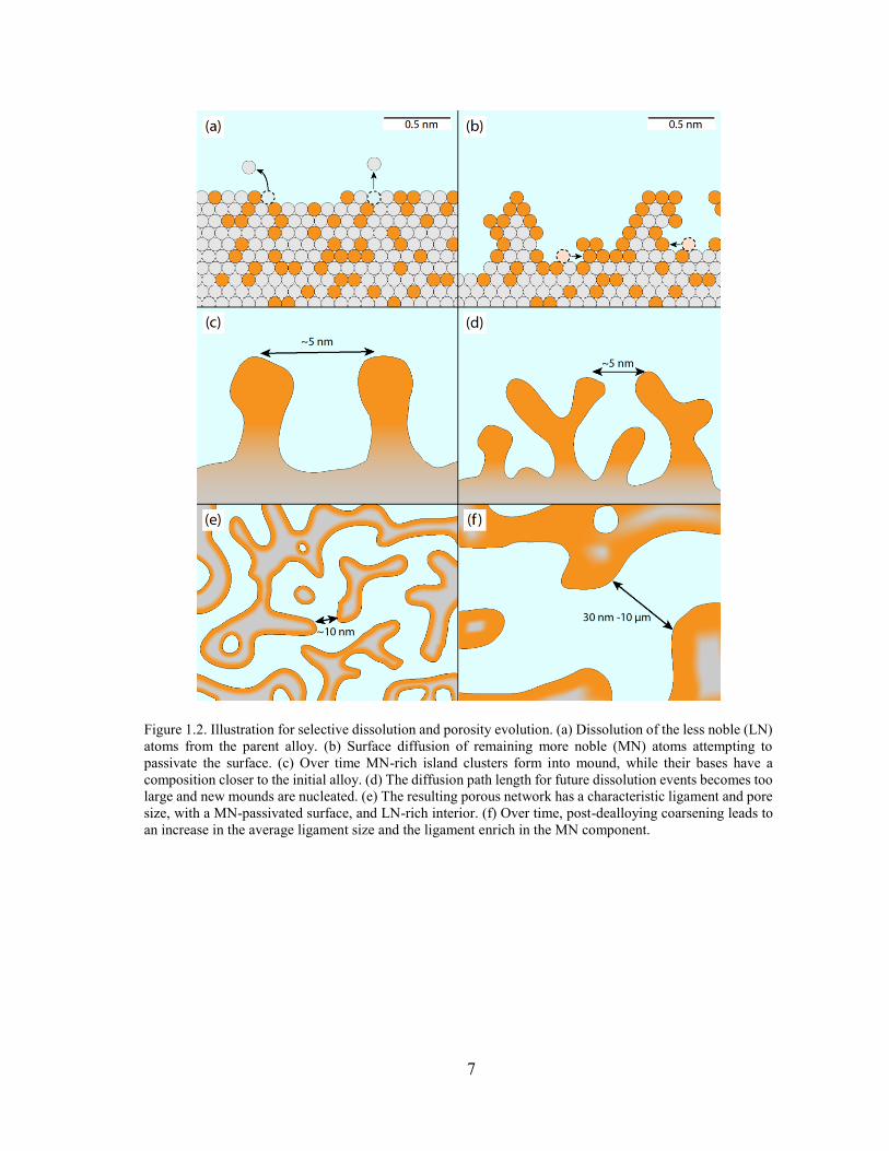
The mechanistic model is illustrated in Figure 1.2. Thermodynamically, dealloying is

favorable above a particular critical electrochemical potential, cV , which balances the free

energy reduction associated with dissolution into solution with the energetic penalty associated

with any new roughness and surface area created (18). During dissolution, LN atoms from low-

coordination surface sites are easily solvated and dissolve into the electrolyte, Figure 1.2a (19).

Dealloying is analogous to crystal growth, where the dealloying interface advances through

layer-by-layer dissolution compared to layer-by-layer growth in thin film systems. It follows

6

that the rate-limiting step of nanoporosity evolution is the dissolution of an atom from a high-

coordination site such as a terrace (20), which leads to the creation of a terrace vacancy that

then grows laterally into a vacancy cluster as lateral near-neighbors are subsequently dissolved.

During dissolution the MN component is left on the surface as adatoms at high

concentrations, Figure 1.2b. Using a regular solution model, it was shown that the equilibrium

concentration of adatoms on the surface is very low (19) and the MN component will diffuse

with the receding step edge. The MN atoms form island clusters, which grow into mounds as

the dealloying process continues, Figure 1.2c. This a type of interfacial uphill diffusion

(adatoms moving from low concentration areas to high concentration areas) mathematically

describable by Cahn-Hilliard diffusion kinetics usually associated with spinodal

decomposition (8). Eventually, the path length for diffusing MN atoms to travel to the MN-

passivated mounds becomes too large and new MN-rich regions develop, bifurcating the pores,

Figure 1.2d. Following this process of mound nucleation and bifurcation, porosity proceeds

into the bulk and a bicontinuous structure is formed with a characteristic ligament and pore

size, Figure 1.2e. At some point, it may be thought that transport of dissolved cations out of

the porous layer becomes rate-limiting, but in practice this diffusion rate is nearly ten orders

of magnitude faster than interface diffusion and electrolyte diffusion has never been observed

to be rate limiting. Nanoporous metals, however, are metastable structures and, if left in

solution, nanoporous metals will undergo post-dealloying coarsening, Figure 1.2f, to reduce

their large interfacial area. As a result, the average ligament size increases and LN atoms left

in the interior of the ligaments are exposed and dissolved. In an extreme case (as t ), the

structure will coarsen into a large lump consisting only of the MN component.

7

Figure 1.2. Illustration for selective dissolution and porosity evolution. (a) Dissolution of the less noble (LN)

atoms from the parent alloy. (b) Surface diffusion of remaining more noble (MN) atoms attempting to

passivate the surface. (c) Over time MN-rich island clusters form into mound, while their bases have a

composition closer to the initial alloy. (d) The diffusion path length for future dissolution events becomes too

large and new mounds are nucleated. (e) The resulting porous network has a characteristic ligament and pore

size, with a MN-passivated surface, and LN-rich interior. (f) Over time, post-dealloying coarsening leads to

an increase in the average ligament size and the ligament enrich in the MN component.

8

1.3 Parting limit critical potential, bicontinuous structure

Historically, dealloying systems have been characterized by two key parameters: the

parting limit, or percolation threshold cp , defined as the fraction of the LN species above

which dealloying occurs, and the critical potential, CV , defined as the minimum potential

required for bulk dealloying. The parting limit and critical potential were defined early in the

development of dealloying theory (21), but the understanding of both concepts have been

refined in the last decade.

1.3.1 The Parting Limit

The parting limit is the critical alloy composition necessary for a structure to fully dealloy;

this does not necessarily imply porosity evolution and only asks the question whether or not

the dissolving liquid can travel from one end of the sample to the other. Another way of

considering this problem is whether there is a network/chain of atoms (of the LN component),

which goes through the entire sample. If the composition is below the parting limit the structure

will not fully dealloy, and if the composition is above the parting limiting it will fully dealloy.

For electrochemical dealloying of AgxAu1-x the parting limit is ~55 at.% Ag, however the

percolation threshold for an fcc lattice is only ~20 at.%. Recent work by Artymowicz showed

that this difference can be explained by considering high-density clusters (22). Specifically,

the study examined the high-density percolation threshold cp m , which denotes that a

percolation chain/path exists composed of Ag atoms with at least m Ag near-neighbors. If we

assume Ag atoms only need one Ag near-neighbor, 1cp , the critical threshold is ~20 at.%.

If, however the number of near-neighbors is increased to nine the threshold isn’t observed until

9

the Ag composition is at least ~ 60 at.%, i.e. 9 60cp (a value very similar to the observed

parting limit). The percolation clusters at these higher concentrations are 2-3 atoms wider than

1cp , and it is thought that there is a geometric requirement for ion solvation; if the chain is

too small the LN component is unable to coordinate with anions in solution and dissolve.

Kinetic factors such as surface diffusion and dissolution can alter the observed threshold,

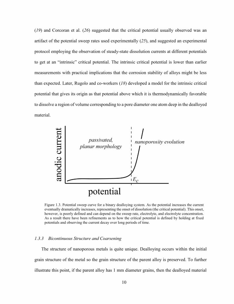
however this has not been extensively studied.

1.3.2 The Critical Potential

The idea of a critical potential, CV , is grounded in the field of corrosion science (10, 23,

24) and is an important concept because it represents the onset of selective dissolution. This

has implications in corrosion and pitting corrosion of the important aluminum alloy 2024 as

well as stress-corrosion cracking in brass and stainless steel alloys (25). The critical potential,

however, is poorly defined by a potential sweep as can be seen in Figure 1.3. It is clear that as

the potential increases, the current - associated with dissolution of the LN component -

eventually increases exponentially. Unfortunately, the exact value of “the onset of selective

dissolution” is unclear; empirically, it has been defined as the value when the current is above

~ 21 mA cm . Going back to our model in section 1.2, the critical potential is the value where

the surface dissolution rate (itself a function of the applied potential) overcomes the passivation

of the MN component (where the surface diffusivity is not a function of applied potential). The

critical potential is a function of alloy composition, typically decreasing with decreasing LN

composition. However, as the composition varies toward 100% of the LN component, the

critical potential does not tend toward the reversible dissolution potential for that element, as

would be expected, and instead was typically a few hundred millivolts higher (18). Erlebacher

10

(19) and Corcoran et al. (26) suggested that the critical potential usually observed was an

artifact of the potential sweep rates used experimentally (25), and suggested an experimental

protocol employing the observation of steady-state dissolution currents at different potentials

to get at an “intrinsic” critical potential. The intrinsic critical potential is lower than earlier

measurements with practical implications that the corrosion stability of alloys might be less

than expected. Later, Rugolo and co-workers (18) developed a model for the intrinsic critical

potential that gives its origin as that potential above which it is thermodynamically favorable

to dissolve a region of volume corresponding to a pore diameter one atom deep in the dealloyed

material.

1.3.3 Bicontinuous Structure and Coarsening

The structure of nanoporous metals is quite unique. Dealloying occurs within the initial

grain structure of the metal so the grain structure of the parent alloy is preserved. To further

illustrate this point, if the parent alloy has 1 mm diameter grains, then the dealloyed material

Figure 1.3. Potential sweep curve for a binary dealloying system. As the potential increases the current

eventually dramatically increases, representing the onset of dissolution (the critical potential). This onset,

however, is poorly defined and can depend on the sweep rate, electrolyte, and electrolyte concentration.

As a result there have been refinements as to how the critical potential is defined by holding at fixed

potentials and observing the current decay over long periods of time.

11

will also have 1 mm diameter grains, where each grain is nanoporous with ligaments

maintaining the same crystal orientation throughout. Nanoporous metals have been compared

to sintered structures, however, this is an incorrect statement because the porous networks are

single crystalline within each grain and lack internal boundaries. Due to this feature, diffusion

pathways are very large. This imparts unique geometric features to nanoporous metals: namely

that they possess regions of positive, negative, and saddle point curvature in a topologically

complex network. Such complex topologies have been of significant recent interest (27–32),

and methods have been developed to describe the topology of nanoporous metals (33, 34),

while the dynamics of topology evolution have been studied by KMC and MD (35, 36).

Coarsening of nanoporous metals is driven by thermodynamic surface energy reduction

(35–37). The results of these studies indicate that structure evolution tends to proceed via

pinch-off Rayleigh instabilities which reduce the local genus (the number of “handles” in the

structure). One implication is that inverse Rayleigh instabilities - a tunnel breaking up into a

series of voids - can also occur, which in turn explain the TEM observations of large voids

within the ligaments of np-Au reported in (38).

1.4 Conditions for electrochemical dealloying/limits of tunability

One reason for the growing popularity of studying dealloyed nanoporous metals is that they

are very easy to make. A homogeneous alloy precursor, of whatever shape or form factor, is

simply immersed into an acid that selectively dissolves one component away. As long as the

remaining component is free to diffuse along the acid/alloy interface, porosity generally forms.

However, the major drawback to this technique is that there are several requirements for

porosity evolution (19):

12

1. The electrochemical reduction potential between the MN and LN components

needs to be several hundred millivolts. For instance, in the Ag-Au system, the

difference between the standard reductions potentials of Ag and Au is ~1V .

However, in the Ni-Cu system – which does not evolve porosity – the difference in

the two standard reduction potentials is ~500 mV . The critical potential of an alloy

system typically sits between the reduction potentials of the two elements; in the

case of Ni-Cu it is difficult to perform selective dissolution, and both elements

simultaneously dissolve. Certain chemical tricks can be used to achieve potential-

independent selective dissolution, but this has only been reported for one system.

2. The parting limit imposes a restriction on the composition range to fabricate a

porous material. Below the parting limit the system is passivated and porosity does

not occur. There is also an upper limit on the alloy composition where if there is

too little of the MN component the structure does not hold together. This is difficult

to predict a priori and the parting limit can vary system to system. For instance, Zn-

Cu systems only require 20 at.% of the LN component for porosity evolution to

occur.

3. The alloying components must form a homogeneous solid solution. This is not a

strict requirement, in fact intermetallic and glassy alloys have been dealloyed, but

these structures do not have uniform ligament sizes. As a result, reporting size-

dependent properties becomes difficult.

4. The final requirement is that the surface diffusivity of the MN component needs to

fall within a certain window, i.e. a Goldilocks Principle: If the surface diffusivity

13

is too low the MN clusters, and subsequent mounds (Figure 1.2), are unable to form.

The system will dealloy but porosity evolution will not occur. Conversely, if the

surface diffusivity is too high the structure will passivate and bulk dealloying will

occur.

Due to these requirements, dealloying has been restricted to noble-metal systems, Figure

1.4, which are often expensive and are limited to catalysis applications. This figure illustrates

the lack of diversity of porous materials at the start of my PhD studies (2010) and will be

compared with the current state of dealloyed materials in Chapter 6.

1.5 Liquid Metal Dealloying

The requirements laid out in section 1.5 demonstrate that although electrochemical

dealloying is an easy technique, it can only be applied to metal systems that meet certain

requirements. Elements that are prone to oxidation, such as Ti or Al, can never be fabricated

Figure 1.4. Periodic table showing the elements (highlighted blue) which have been successfully

fabricated into nanoporous metals via dealloying. Note that all of the elements are noble metals,

demonstrating the limitations of current dealloying techniques.

14

by electrochemical techniques, and atoms with slow surface mobilities (e.g. Ta, W), will not

diffuse fast enough to form porous structures. The concept of dealloying has recently been

generalized to be any form of liquid-mediated dissolution, representing a paradigm shift in this

community.

Harrison & Wagner (39) first examined this idea in 1959 by looking at metal alloy

corrosion in molten metals and salts, but this idea did not catch on until Kato and coworkers

(40) reported making porous Ti in 2011 by dealloying Ti-Cu alloys in molten Mg. Analogous

to the critical potential, the dissolving component has a negative enthalpy of mixing with the

liquid phase, which thermodynamically drives the dissolution process. Unlike electrochemical

dealloying, dissolution is always favorable and there is no critical potential. Preliminary studies

of liquid metal dealloying (LMD) have shown that the morphologies are similar to

electrochemical dealloying, which is to be expected as long as the two competing mechanisms

(dissolution and surface diffusion) are the same (41, 42). We will come back to this concept in

Chapter 3 for the development of new alloy systems.

1.6 Mechanical Properties

Nanoporous metals are an attractive material for structure applications because they consist

of ~1018 nanoscale objects (for 10 nm ligaments in 1 cm3 of material), and should have similar

size-dependent strengthening – increasing strength with decreasing size – as is seen in

micropillar and nanowire systems. The wealth of the work on the size-dependence of the yield

strength in nanoporous metals has been performed on np-Au, however, the scaling laws are

expected to be the same for all bicontinuous nanoporous metals. The mechanical properties of

np-Au have been examined by many research groups using a variety of mechanical techniques

15

including tension, compression and hardness testing (43–69). A compilation of the data is

given in Table A.1 and Figure 1.5. There is significant scatter (addressed below), however the

data demonstrates an overall increase in strength with decreasing ligament size, suggesting that

there is an expression to relate the strength of the porous material to its feature size.

16

Figure 1.5. Yield strength versus ligament size for reported values of np-Au in the literature from various

mechanical tests: hardness values (square), compression values (circle), thin film stress values

(pentagon), tension values (triangle), simulation values (diamond), and deflection tension testing

(upside-down triangle). It is apparent that there is a trend of increasing strength with decreasing ligament

size, however there is a large amount of scatter associated with samples having different relative

densities.

17

1.6.1 Scaling Laws and Gibson-Ashby Relations

Despite being a network of connected nanostructures, nanoporous metals are still high-

density foams and have decreased mechanical properties compared to their fully dense

nanowire, micropillar, or nanocrystalline counterparts. The underlying strength of nanoporous

metals are commonly estimated using the empirical Gibson-Ashby (GA) relations for foams

(70). The GA equations for the yield strength and elastic modulus of a foam are given by

n

foam bulk

y yC

(1.1)

Enfoam bulk

EE C E (1.2)

Here, C and EC are geometric constants taken to be 0.3C and 1.0EC , bulk

y and

bulkE are the bulk yield strength and elastic modulus, is the relative density of the material

( foam bulk ), and both n and En are exponents dependent on the microstructure of the

solid material, but taken to be 3 2 and 2 , respectively, for bending-dominated behavior.

It has been noted in simulations by Sun et al. (71) that ligaments in np-metals undergo both

bending and tensile deformation, and the values for C , EC , n , and En need to be carefully

considered when being applied to a particular system of materials. The values of C and n

will be addressed in Chapter 5.

Previous work by Hodge and coworkers (46, 49) expressed the size-dependence using a

Hall-Petch relationship, but individual ligaments are not constrained by adjacent grains and the

ligaments are more aptly compared to micropillars/nanowires as suggested by several other

research groups (43, 57, 61, 66, 67). The equation for the yield strength as a function of

ligament size is given by

m

y o A , (1.3)

18

where o is the scale-independent yield strength, is the ligament size, and A and m

are empirical constants. The first term is very small and can be neglected (72), and the yield

strength becomes

m

y A . (1.4)

Combining the yield strength and Gibson-Ashby relation yields the equation

n

foam m

y C A

. (1.5)

Note, however, that the power-law relationship is grounded in statistics. Specifically, the

power-law relationship in micropillars is linked to the probability of finding the maximum size

of a dislocation source in a material with a given diameter and dislocation density, as discussed

in recent work by El-Awady, who established a size-dependent Taylor-strengthening law for

dislocation-mediated plasticity in micropillars (73). El-Awady points out that the

strengthening mechanism relies heavily on the dislocation density in the material and, in the

case of plasticity, knowledge of the kinetic evolution of the dislocation density of the material

during deformation. Unfortunately, to our knowledge there have only been two qualitative

studies of dislocation microstructure in micropillars (74, 75), let alone for nanoporous metals,

and we cannot compare Eq. (1) with this more rigorous model.

There is no size-dependent scaling law for the elastic modulus of nanoporous metals

because it is not expected to change dramatically above 10 nm as pointed out by Weissmuller

et al. (48). Large sample (mm-scale) experiments have shown dramatic manifestations of

elastic behavior such as macroscopic actuation caused by electrocapillary forces (changes in

surface stress with applied electrochemical potential) in solution and gas-phase environments

(3, 76–80).It has been suggested that excess elasticity on the surface might decrease or increase

the elastic modulus, and was reported in simulations of materials with 2-4 nm ligaments by

19

Sun et al. and Farkas et al. (62, 71), but experiments in nanoporous metals generally show no

change in modulus. One set of experiments by Mathur & Erlebacher inferred the modulus of

np-Au by examination of the buckling of thin films (81), showing an increase in the modulus

with decreasing ligament size, but the authors argued that it was a geometric manifestation and

did not originate from the ligaments. The effects of capillary forces and altering the surface

stress of nanoporous metals have been discussed in detail previously and can be found in

Reference (48) and those therein.

1.6.2 Dislocation Activity

Dislocation activity in nanoporous metals is expected to be different because individual

ligaments are observed to be ductile, but the bulk structure tends to be brittle (at least in

tension). This was first observed in a fracture toughness study by Li and Sieradzki (82) where

a ductile-brittle transition was observed in np-Au when the sample size was significantly larger

than the ligament size. Pure tension tests confirmed this brittle behavior (58, 61, 69),

contrasting with the ductile behavior observed in compression and hardness testing. This

tension-compression asymmetry was observed in MD simulations by Farkas et al. (62), but

only for ligaments below 15-20 nm and was attributed to the surface stress response of the

ligaments.

TEM experiments, MD simulations, and an EBSD study all showed significant dislocation

activity inside the ligaments, even at sizes as small as 3 nm (60, 62, 63, 67, 71). Due to the

small ligament sizes in these samples, perfect dislocations are not observed but there is a large

density of twins, stacking faults, and Shockley partial dislocations. MD simulations showed

that Shockley partials are emitted from the surface, and quickly pass through ligaments, leaving

20

behind twins and stacking faults. TEM studies confirm these observations and noted that this

behavior is similar to pure Au wires 50 nm in diameter. In fact, dislocations don’t always

terminate on the surface, and can move through ligaments and eventually into nodes. An EBSD

study on 55 nm ligament np-Au by Jin and coworkers (56) demonstrated the evolution of a

dislocation cell structure, suggesting dislocations in porous metals were able to move a

distance larger than the ligament diameter and can be stored.

All of this work suggests that nanoporous metals are ductile, at least locally, and it is

difficult to have coherent, macroscopic plasticity where a dislocation can travel large distances

though the highly porous network. Dislocations easily terminate on surfaces and uniform

deformation is impossible. This informs understanding of the brittle behavior in tension,

whereas compression testing masks this lack of coherency either through densification or

inherently preventing early catastrophic failure. We will discuss these limitations and design

strategies for new bicontinuous structures in Chapter 5.

21

Chapter 2 Dealloying in Finite Systems

2.1 Summary

In this chapter we examine dealloying in binary nanoparticles in order to understand how

porosity evolves in confined systems where the chemical potential term dominates. The Gibbs-

Thomson effect (the reduction of local chemical potential due to nanoscale curvature) predicts

that nanoparticles of radius r dissolve at lower electrochemical potentials than bulk materials,

decreasing as 1 r . However, we show here that if the particle is an alloy –susceptible to

selective dissolution (dealloying) and nanoporosity evolution – then complete selective

electrochemical dissolution and porosity evolution requires a higher electrochemical potential

than the comparable bulk planar material, increasing empirically as 1 r . This is a kinetic

effect, which we demonstrate via kinetic Monte Carlo (KMC) simulation. Our model shows

that in the initial stages of dissolution, the less noble particle component is easily stripped from

the nanoparticle surface, but owing to an increased mobility of the more noble atoms, the

surface of the particle quickly passivates. At a fixed electrochemical potential, porosity and

complete dealloying can only evolve if fluctuations in the surface passivation layer are

22

sufficiently long-lived to allow dissolution from percolating networks of the less-noble

component that penetrate through the bulk of the particle.

2.2 Background

Porosity evolution can occur during dealloying when the dissolution rate is fast enough

relative to the surface diffusion rate of the undissolved component, with ligament and pore

sizes in some cases less than 5 nm. Dealloying has been used to fabricate bulk metals for

catalysis with high surface areas, however this form factor is not always useful (12, 83, 84). In

the case of bulk np-NiPt, the mass activity for oxygen reduction drops as porosity extends into

the bulk of the material. A function of the overpotential, oxygen will diffuse an average

distance before being reduced to water. This suggests that there is an optimum dealloying depth

for a porous catalyst and it is useful to consider finite systems. In the case of a nanoparticle,

the diameter can be finely tuned and it can be dealloyed to produce a nanoporous nanoparticle.

Dealloyed nanoparticles are potentially excellent electrocatalysts (85, 86), combining the

high surface area/volume features of traditional nanoparticles with the ability to tune

composition and morphology for improved functionality. Nanoporous particles offer

additional functionality because the porous region can be filled with secondary phases to form

nanoreactors (12). Nanoporous metals generally exhibit unusual physical behavior associated

with their structure including nanoscale manifestations of thermodynamic surface stress (87)

and high magnetoresistance (88). Typically dealloying of nanoparticles is accomplished by

electrochemical potential cycling between prescribed voltage limits, sometimes yielding a

variety of dealloyed nanoparticle types including core-shell and nanoporous structures.

23

Thermodynamically, dealloying is favorable above a particular critical electrochemical

potential Ecrit that balances the free energy reduction associated with dissolution into solution

with the energetic penalty associated with any new roughness and surface area created (18).

The energy gain associated with electrochemical dissolution is a strong function of the

curvature of the surface, and for single component materials the electrochemical potential

decreases with particle radius r as a function of 1/r due to the Gibbs-Thomson effect (89, 90).

The electrochemical stability of nanoparticles has been previously studied, and the relationship

for the dissolution voltage (in millivolts) is given as:

2nn

M MM M

M ME r E r

nF

(2.1)

where nM ME r is the size-dependent standard reduction potential of the metal species M,

nM ME is the bulk standard reduction potential, M is the surface energy, M is the molar

volume, n is the number of electrons per mole product, F is the Faraday constant, and r is the

radius of the nanoparticle. Using standard values for 2 2Pt e Pt , the relationship

becomes:

2 1011 133 2Pt Pt

E r mV (2.2)

An experimental plot of the stability of Pt nanoparticles can be seen in Figure 2.1. The effect

does not become dramatic until the radius is smaller than 2 nm, however there is a 200 mV

difference between the bulk value and a 2 nm radius particle, which is significant for an

industrial application.

24

It might be expected that the potential at which porosity forms in a nanoparticle should also

decrease with decreasing radii, but here we report the results of kinetic Monte Carlo

simulations (KMC) showing that this potential actually increases with 1/r in alloy

nanoparticles. The origin of this effect lies in the details of nanoparticle alloy dissolution –

generally, regardless of potential, dealloying nanoparticles initially and quickly tends to form

noble-metal passivated particles. Porosity only forms over longer timescales if the dissolution

rate is high enough to form pits during transient surface fluctuations that expose less-noble

atoms buried under step edges to the external environment. Such surface fluctuations increase

in frequency but decrease in duration with smaller particle size because of the rise in surface

mobility associated with the Gibbs-Thomson effect (such fluctuations can be considered the

initial manifestation of the melting point suppression in nanoparticles).

Figure 2.1. Electrochemical dissolution potential versus 2 r for Pt nanoparticles from Ref. (89). This

decrease in stability reflects a lower limit on Pt nanoparticle size for catalytic applications.

25

2.3 Experimental Methods

To study selective dissolution in alloy nanoparticles, we used the KMC simulation code

MESOSIM, a full description of which can be found in Ref. (19). Briefly, MESOSIM has

been optimized to reflect time and energy scales associated with the prototypical Ag-Au

dealloying system (leading to np-Au), but the general trends here should be applicable to

dealloyable systems that remain single phase. Simulations are initialized by placing atoms on

a 3-dimensional fcc lattice and the type of atom (Ag or Au) is assigned at random based on a

weighted probability determined by the composition of the alloy. The time evolution of the

system is governed by the KMC algorithm. In KMC, if there are N total events that can occur,

each one indexed by i and possessing rate ki , the time for a single event to occur is

1

lnN

i

i

t k

where ξ is a random number in (0,1]. Within this time the probability of an

event occurring is 1

1

N

i i j

j

P k k

. KMC simulations progress by picking a random event

according to its weighted probability (more unstable events are weighted heavier than stable

ones) and then the time is incremented accordingly. Our model here draws on the model

introduced in Ref (91) and uses a simple bond-breaking model to capture the generic

morphological evolution physics occurring over experimental timescales. Specifically, rates

for surface diffusion and dissolution at a potential are given by the expressions

1 exp Bdiff

b

nEk v

k T

, and 2 exp B

diss

b

nEk v

k T

, where

13 1

1 10 secv , 4 1

2 10 secv ,

0.15eVBE for all bond energies, and n is the number of bonds. These parameters have

been shown in other studies to accurately model dissolution current vs potential behavior (8,

91, 92) the parameters also successfully model coarsening in nanoporous nanoparticles (35)

26

that agree with timescales of experimental studies of coarsening of np-Au (which we note are

generally much longer than any of the timescales discussed in this work) (93); and recently an

experimental measurement of the activation barrier for dissolution of Ag from a terrace site

was measured, and found to be consistent with a bond energy between 0.1-0.2 eV (20).

2.4 Results and Discussion

Figure 2.2 shows a representative time evolution of a simulated nanoparticle of radius

30 and composition 75 at. % Ag. Overall, three different compositions were examined: 65,

75, and 85 at. % Ag; and four different nanoparticle radii: 8, 11, 18, 30 1 atom diameters.

These values approximately correspond to nanoparticle diameters of ~4, 6, 10, and 17 nm. The

compositions were chosen to be representative of the composition range typically found in

porosity-forming dealloying systems (8, 19). Smaller particles were not studied because the

roughness that evolved in the initial stages of dissolution was greater in amplitude than the

particle diameter, and porosity never evolved. Particles were dealloyed under constant

potential at 300K and ran between 104-105 simulated seconds or ~5x108 iterations. The

behavior exemplified by the particle in Figure 2.2 shows the following characteristics: (a) at

short times, t < 102 sec., the outmost silver atoms are quickly stripped. Unlike the case of a

bulk, planar surface, there are always low-coordination Ag atoms sitting at step edges at facet

boundaries that facilitate such stripping; (b) at intermediate times t < 103 sec. , the particle is

passivated with a monolayer of gold, which surface diffuses until the particle approaches the

equilibrium Wulff shape (if we start the simulations with particle shapes already equilibrated

to the Wulff shape rather than a sphere, our results are unchanged); (c) over long time periods,

regions of the bulk are exposed to the external environment due to fluctuations in the outermost

27

layer; (d) in some cases, these fluctuations are long-lived enough to allow further attack into

the interior of the nanoparticle. An important point here is that fluctuations exposing the

interior also appear in stage (a), but the concurrent dissolution of the outermost silver is

roughening the surface so quickly that there are always nearby gold atoms that can diffuse into

terrace vacancies resulting in transient passivation.

In dealloying of bulk planar materials, the critical potential is a sharp threshold

separating porosity formation from surface passivation (25). Analogously in nanoparticles, we

find an increase in the propensity for porosity evolution to exist as the electrochemical potential

Figure 2.2. Time evolution of a simulated Ag-Au (white spheres: Ag; dark spheres: Au) nanoparticle (r

= 30, 75 at. % Ag) under constant potential ( 0.98 eV ). Initially the surface is Ag rich; it is easily

stripped off and the surface roughens. The remaining Au atoms quickly form a passivating monolayer

and a pseudo-equilibrated Wulff shape; eventually, a long-lived surface fluctuation reveals a percolating

network of silver atoms in the bulk that dissolves to form a nanoporous nanoparticle.

28

increases, but this threshold is not sharp. To quantify this observation, for each particular

radius and electrochemical potential we generated a histogram over the course of many runs

(Figure 2.3), typically many thousand, showing the final volume of the particle after being

subjected to a dissolution potential for some fixed, but long, period of time (104 sec).

Near a potential for porosity evolution PE , distinct from and larger than the critical potential

for the bulk planar alloy, we see two Gaussian distributions corresponding to two final particle

volumes. The distribution at smaller volume corresponds to fully dealloyed and porous

particles that have lost the majority of their less-noble component mass, and the other

corresponds to particles that have undergone only superficial surface dealloying and become

passivated with the noble component. For this latter case, there is still a significant amount of

Figure 2.3. Histogram data of 2000 runs of a r = 18 particle, 85 at. %Ag, under constant dissolution

potential 0.975 eV . The Gaussian at smaller number of atoms corresponds to dealloyed and porous

nanoparticles while the Gaussian at larger number of atoms corresponds to passivated, but non-porous

nanoparticles. The initial number of atoms for this particle radius was approximately 43.68 10 .

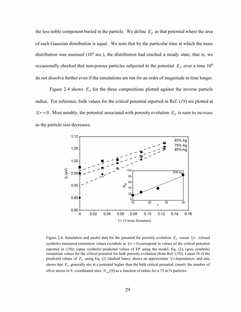
29

the less noble component buried in the particle. We define PE as that potential where the area

of each Gaussian distribution is equal. We note that by the particular time at which the mass

distribution was assessed (104 sec.), the distribution had reached a steady state; that is, we

occasionally checked that non-porous particles subjected to the potential PE over a time 104

do not dissolve further even if the simulations are run for an order of magnitude in time longer.

Figure 2.4 shows PE for the three compositions plotted against the inverse particle

radius. For reference, bulk values for the critical potential reported in Ref. (19) are plotted at

1 0r . Most notably, the potential associated with porosity evolution PE is seen to increase

as the particle size decreases.

Figure 2.4. Simulation and model data for the potential for porosity evolution PE versus 1 r . (closed

symbols) measured simulation values (symbols at 1 0r correspond to values of the critical potential

reported in (19)); (open symbols) predicted values of EP using the model, Eq. (2); (grey symbols)

simulation values for the critical potential for bulk porosity evolution (from Ref. (19)). Linear fit of the

predicted values of PE using Eq. (2) (dashed lines), shows an approximate 1 r dependence, and also

shows that PE generally sits at a potential higher than the bulk critical potential. (inset): the number of

silver atoms in 9- coordinated sites 0AgN as a function of radius for a 75 at.% particles.

30

This observation should not be interpreted to mean that it is more difficult energetically to

dissolve silver atoms from smaller particles than from larger ones. All the particles here

quickly lose silver from their initial surface, and, in accordance with the Gibbs-Thomson

effect, at fixed potential smaller particles tend to lose their surface silver more quickly because

they have a higher fraction of low-coordinated step and kink sites (90). However, for the same

reason, the gold atoms left behind on the alloy particle surface are much more mobile on the

smaller particles and thus quickly passivate the interior. It is possible that reduction of the

ratio diff dissk k could reduce such passivation at a fixed particle size and potential, but it is

unclear how to experimentally achieve this.

We necessarily conclude that PE is fundamentally kinetic in origin, containing a

complex choreography of surface composition fluctuations convoluted with the geometric

connectivity of the more reactive component under the passivating gold surface. The

ingredients that need to be included in a kinetic model for PE include:

(i) An observation that the initial stage of porosity evolution in particles must be gold-

passivated particles and not a surface with an appreciable concentration of silver. After this

initial stage, there are a few silver atoms exposed on the surface on the low-index facets, but

the majority of silver atoms still on the surface sit along facet boundaries in 10- and 11-

coordinated sites (see, for instance, Figure 2.5). For this reason, the number of exposed silver

atoms at this stage of evolution increases approximately linearly with the particle radius.

31

(ii) The majority of surface diffusion events that can lead to further exposure of silver

to the electrolyte, or reduction of silver coordination, are fluctuations at step edges that reduce

the coordination of 10- and 11-coordinated silver atoms to 9-coordinated terrace sites

susceptible to attack by electrolyte. Over long periods of simulated time, of order 104 sec,

many Ag atoms are transiently exposed to the electrolyte. The 9- coordination number

corresponds geometrically to a terrace atom in a (111)-oriented surface, and it has been shown

that this is likely the maximum coordination for which dissolution occurs (20, 22); physically,

more highly coordinated atoms are thought not to be sterically complexable by anions in

solution. Within the model, the lifetime of the fluctuation exposing Ag atoms is independent

Figure 2.5. Snapshots of passivated particles as a function of particle size. As the particle size increases

the fraction of silver atoms on terrace sites decreases and the majority are found underneath step edges.

32

of the dissolution potential. At the very least, for porosity to form, this lifetime must be larger

than the average time to dissolve silver from such a terrace site (Figure 2.6).

(iii) Finally, assuming the Ag atom is dissolved within the lifetime of a surface

fluctuation, porosity can form only if the surface Ag atom is connected to a percolation network

of other Ag atoms through the bulk of the particle. In contrast to the early stages of dissolution,

Figure 2.6 Surface fluctuation lifetime data for r = 8 particles (top) and r = 30 particles (bottom). The

time interval t is the lifetime of a 9 Ag atom coordinated terrace site. The peak at 6~ 10 sec.

corresponds to surface fluctuations associated with adatom motion, and the peak at ~10 sec. corresponds

to fluctuations at kink sites. We set kinkt to the center of the latter peak, and the area under the kink

distribution to kinkP .

33

where there are many Au atoms diffusing on the surface that are readily available to passivate

low-coordinate surface defects, the surface vacancies associated with dissolution of silver

atoms during these surface fluctuations are very long-lived. As a result, we observe that if a

percolation network of silver atoms starts to dissolve after the particle has reached the pseudo-

equilibrated Wulff shape, the entire particle will almost instantaneously dealloy and become

porous. It can be seen in Figure 2.7 that the error associated with the probability a surface atom

is connected to a percolation network becomes quite large as the particle size decreases. This

is result of having a finite system and represents the length scales below which the existence

of high-density percolation networks disappears. This results in a distribution of dealloyed

morphologies in nanoparticles including porous, core-shell, and passivated nanoparticles

Figure 2.7 Probability that a surface silver atom is connected to a percolation pathway in the nanoparticle.

If this atom is selected to dissolve the entire particle will evolve porosity. This probability is weakly size-

dependent, but most importantly dependent on the alloy composition.

34

Taken together, these observations lead to a first order master equation describing the rate

of change of the number of exposed 9-coordinated silver atoms AgN :

Ag

Agdiss kink perc

dNk P P N

dt (2.3)

Here, dissk is the dissolution frequency from a 9-coordinated site, kinkP is the probability a

kink site has fluctuated with large-enough amplitude to expose a silver atom, and percP is the

probability this silver atom is connected to a percolation network into the bulk. Because a

single dissolution event at this stage tends to lead to porosity evolution, the simplest criterion

for PE is determined by the condition that over a period of time t equal to the lifetime of the

step edge fluctuation the surface silver concentration decreases by one: 0 1Ag AgN t N

. Solving Eq. (2.3) under this condition and noting that the simulation rule

exp 9diss B P Bk E E k T , we find PE is determined by

0 119 ln ln

0

Ag

P B b

kink perc Ag

NE E k T

vP P t N

(2.4)

The simulation model allows percP , 0AgN , kinkP and t to be quantitatively measured

independently. For percolation and 0AgN , particle dissolution was halted upon completion

of the passivation layer, and 9-coordinated silver atoms were counted and checked to see

whether or not they belonged to a percolation network. A high-density percolation (HDP)

threshold criterion was used to determine if a silver atom belonged to a percolation network,

following Ref. (22), requiring Ag atoms to be counted in the percolating network if at least

nine of its twelve potential neighbors are also silver. As discussed in Ref. (22), this criterion

35

is equivalent to the physically reasonable requirement that there be enough free volume around

a surface silver atom for it to be solvated and dissolved by the electrolyte. Not surprisingly

over the particle sizes examined, we find little size dependence of the probability of belonging

to such a percolation network, with the probabilities equaling ~42%, ~81%, and ~97%, for

compositions of 65, 75 and 85 at. % Ag, Figure 2.7. For 0AgN , we find a weak linear

dependence (see inset of Figure 2.4) on the particle radius, reflecting how most of the exposed

silver atoms sit on facet boundary regions, the length of which increases linearly with particle

radius.

The largest particle size-dependence is found for kinkP and t , the measures associated

with fluctuations that lead to transient exposure buried of surface silver atoms. To quantify

this effect, gold-passivated particles were again generated, but then silver atoms were not

allowed to dissolve or diffuse during the further course of the simulation. These simulations

tracked the time interval between a silver atom becoming 9-coordinated, and then becoming

buried (i.e., re-passivated) by surface diffusing gold. Histograms of these time intervals for

radius 8 and radius 30 particles are shown in Figure 2.6, and exhibit a rich complexity. For

both particle sizes shown, we see that the majority of fluctuations are short-lived – 10-6 to 10-

7 sec. – with a slight shift as the size increases to radius 30. These fluctuations are associated

with gold adatoms moving over silver atoms embedded in terraces. Longer-lived fluctuations

are associated with surface diffusion of gold with increasing coordination, so, for instance, the

peak centered around 1 to 10 seconds corresponds to particular fluctuations of interest

involving atoms at kink sites that expose 9-coordinated silver atoms. The difference in

frequency distribution with particle size is straightforwardly explained as a Gibbs-Thomson

effect: Surfaces on the 8r particles are extremely unstable and Ag terrace passivation is

36

controlled by adatom events, but as the radius increases the concentration of highly mobile

low-coordination surface atoms decreases and a majority of the passivation events become

controlled by lower-coordination surface atoms participating in attachment/detachment events

at kink sites. As the longer-lived fluctuations are the ones that ultimately lead to porosity

evolution, we associate kinkP and t with the longer-lived kink-site fluctuations, kinkP being

the area under the peak associated with kinkt .

Using the independently measured values for the time interval, percolation and kink

probabilities, and terrace concentration data into Eq. (2.4) we find good agreement with the

model and the measured values of PE (see Figure 2.4). The slopes for both the simulation and

analytical models for 65 and 75 at.% Ag are approximately the same, but the slope for the 85

at. % simulation data is steeper than that predicted by Eq. (2.4). We resolve this discrepancy

by noting that at high silver fractions, the pseudo-Wulff particle has approximately 15% of its

surface silver atoms on (001) facets, in addition to the majority (111) positions. This means

the average activation barrier for dissolution in this case is slightly smaller than 9 b PE E . In

fact, we find good agreement between model and simulation using 8.9 b PE E in Eq. (2.4) at

the 85 at. % composition, as shown in Figure 2.4.

2.5 Conclusions

The work presented in this chapter impacts tuning the composition and morphology of

dealloyed nanoparticles in the following ways. First, it may require surprisingly high

electrochemical potentials to both fully dealloy a nanoparticle and ensure that every particle in

a batch is porous. In experiments, this is often accomplished by electrochemical cycling which

has the effect of “artificially” increasing the magnitude, lifetime and frequency of surface

37

compositional fluctuations. Second, the work here suggests that stymieing the surface mobility

of the more noble (passivating) component can lead to more facile porosity evolution in

nanoparticles, perhaps by adsorbing a self-assembled monolayer or dealloying under

conditions where this component forms a stable oxide (94, 95).

To summarize, the size dependence of surface site duration, percolation probability,

and concentration of surface sites has been examined for binary alloy fcc nanoparticles. A first

order rate equation provides a reasonable explanation of the increase in the electrochemical

potential necessary for porosity evolution, and we identify the primary source of the increase

to be a Gibbs-Thomson effect acting upon the gold-passivation layer on the particle. While

for small particles there are many small fluctuations in the surface morphology, these

fluctuations are too short-lived to lead to further dissolution. Porosity evolution occurs when

fluctuations are long-enough lived to allow silver dissolution, and surface fluctuation lifetime

increases with particle radius. The results presented in this chapter have been published in (96)

38

Chapter 3 Liquid Metal Dealloying: A New Concept in Porosity

Evolution

3.1 Summary

Dealloying is typically considered an electrochemical process, but corrosion can occur in

a variety of liquid environments, including liquid metals and molten salts. Liquid metal

embrittlement is relevant for a variety of applications, such as galzanized coatings, solders,

brazes, and weld-metals (97–100), but the concept of using this process for porosity evolution

has never garnered interest or been extensively studied. In this chapter we challenge the notion

that dealloying is restricted to electrochemical systems, and extend liquid metal corrosion to

the fabrication of porous structures.

3.2 Background

3.2.1 Liquid Metal Dealloying

Liquid metal embrittlement is generally concerned with grain boundary weakening, and

the accepted mechanism is that the liquid metal forms an intermetallic compound with the

39

parent metal at the grain boundary, destroying the internal interface and lowering the energy

of the system (97–100). This field of study focuses on corrosion along grain boundaries and

not within the grains themselves, and only considers alloy systems where the concentration of

the dissolving component is very low. The idea of using a liquid metal to selectively dissolve

a binary alloy (where the concentration of the dissolving component is higher) was introduced

by Harrison & Wagner in 1959 when they dissolved noble metal alloys such as Cu-Au and Cu-

Ni in metal baths of Bi and Ag, respectively (39). They observed a rough interface and the

formation of a porous structure but this idea did not catch on as a fabrication method –

presumably because the ligaments of the porous structure were hundreds of microns. As a

result the idea remained untouched until 2011 when Kato and coworkers fabricated porous Ti

using liquid Mg as a dealloying medium. As mentioned in Chapter 1, it is very challenging to

fabricate porous materials out of elements with low standard reduction potentials such as Ti;

there are very few alloying components that have a substantially lower reduction potentials

and elements in this reduction potential range are prone to oxidation, inhibiting porosity

evolution.

Another drawback to electrochemical dealloying mentioned in Chapter 1 is that the

surface diffusivity of the remaining component cannot be too fast or too slow. To illustrate this

point, a primary goal of this dissertation was to fabricate porous Ta by electrochemically

dealloying V-Ta precursors (Figure 3.1). This alloy system met the first three requirements

listed in section 1.4, however (in the opposite case of Chapter 2) the surface diffusivity of Ta

was too low for porosity to evolve. A recent publication by Chen & Sieradzki provided a

framework for porosity evolution as a function of the homologous temperature (reaction

temperature normalized by the element’s melting point), demonstrating that Pt is the highest

40

melting point element that can be fabricated at room temperature using electrochemical

dealloying (101). Unfortunately, this work was not published until three years after this

electrochemical dealloying experiment and there was no literature value for the surface

diffusivity of Ta in electrolyte solutions. As a result, we did not fully understand the challenges

of electrochemically dealloying V-Ta alloys and why porosity evolution did not occur.

Liquid metal dealloying (LMD) overcomes this surface diffusivity challenge because the

homologous temperature is much higher – metals are liquid at temperatures hundreds of

degrees higher than electrolyte solutions – which enables porosity evolution. Instead of a

critical potential, LMD uses enthalpies of mixing to control dissolution (41, 42). Specifically,

the liquid metal is chosen to have a negative enthalpy of mixing with the dissolving

component(s) and a positive enthalpy of mixing with the remaining component(s). A schematic

of LMD can be seen in Figure 3.2. Kato & Wada have since published several manuscripts

Figure 3.1. Failure of dealloying V-Ta. This systems meets the first three requirements of laid out in

section 1.4: (a) Ta and V have a large distance between their onset potentials (greater than 1V ), is a

solid solution, and we should expect to see dealloying over a similar composition range as the Ag-Au

system. (b) The fault of this system is that the surface diffusion rate is too slow and the alloy falls apart

when V is dissolved. The dark region is undealloyed Ta-V, and the white region is cracked Ta.

41

describing different LMD systems, focusing on dealloying in molten Mg to produce porous

Fe, Cr, Nb, and Si.

3.2.2 The Ti-Refractory Element System

The remainder of the chapters in this thesis are centered on Ti-X alloys. Using Kato’s work

as inspiration we developed a unique liquid metal dealloying system by immersing Ti-rich

refractory alloys into liquid Cu. Parent alloys of Ti-X, where X is a refractory element/alloy

(e.g., W, Re, Os, Mo, Nb, V), are immersed in a bath of molten Cu. Cu has high Ti solubility

but is immiscible with X. This concept is easily understood by examining a collage of Ti-Ta-

Cu binary phase diagrams, Figure 3.3. Molten Cu dissolves Ti out of the alloy while allowing

the refractory component to diffuse along the metal/liquid interface and reorganize into a

porous network. Copper remains in the pores and fills the dealloyed phase volume as it

penetrates into the parent alloy. The dissolved Ti diffuses out of the sample into the much

larger Cu bath, which acts as a reservoir, effectively diluting it within the composite. After the

dealloying process is completed, a dense bicontinuous composite with a characteristic ligament

Figure 3.2. Schematic of liquid metal dealloying. (a) Parent alloy (dark gray) is immersed into a liquid

metal bath (orange). (b) Zoom-in of the dashed region in (a) showing the dealloyed region (light gray)

and the direction of the dealloying front (into the parent alloy).

42

diameter is formed upon cooling. A nanoporous structure can be excavated by

electrochemically dissolving the Cu phase, and the low surface mobility of Ta at room

temperature in an electrolyte prevents the material from coarsening while sitting in solution.

Referring back to the idea of the homologous temperature, the ligament size can be tuned by

altering the temperature of the bath. Generally, micron-sized ligaments are formed in Cu melts,

but we can fabricate smaller ligaments by adding constituents to the bath, lowering its melting

point. Specifically, by adding Ag and Bi to molten Cu we can fabricate molten baths with

lower melting points across the range 400-1000 oC.

Our dealloying strategy is general to all the refractory elements, but this chapter focuses

on Ti-Ta and Ti-W alloys. It should be clarified that the bicontinuous structure is the result of

a pattern forming instability during dealloying (identical to electrochemical dealloying) and all

of the parent Ti-X alloys are homogenous, solid solution BCC alloys across the composition

range at all processing temperatures.

Figure 3.3 Relevant phase diagrams to understand liquid metal dealloying to make np-Ta. (left) Ti/Ta;

this system forms a homogeneous solid solution over its entire composition range. (center) Ti/Cu; during

LMD, Ti is dissolved from the Ti/Ta ingot and dissolved (up to 70 at. %) in molten Cu alloys. (right)

Ta/Cu; during LMD, the remaining Ta does not dissolve in Cu, even molten copper, and reorganizes itself

into a porous network via interface diffusion between itself and the melt.

43


Ti65Ta35, Ti75Ta25, Ti85Ta15, and Ti75W25 (99.9 wt.% Ti, 99.9 wt.% Ta, and 99.9 wt.% W)

alloy buttons were prepared via arc melting Ti, Ta, and W powders by the Materials

Preparation Center at Ames Laboratory, which is supported by the US DOE, Basic Energy

Sciences. A ~30g Ti95Ta5 alloy was prepared in-house by radio-frequency (RF) induction using

an Ambrel Ekoheat 45 kW system by melting Ti (99.995 wt.%), and Ta (99.95 wt.%) pellets

from Kurt Lesker in a water-cooled copper crucible from Arcast Inc. under flowing Ar (99.999

wt.%). 1 cm3 (~9 g) ingots were cut using wire electrical discharge machining (EDM), and

then annealed via induction melting in an ultra-high vacuum (10-8 torr) environment at ~ 1500

oC for 72 hours in a ultra-high purity alumina crucible cast in-house using materials from

Cotronics Corp. These ingots were then rolled into a foil 150 micrometers thick and 1-cm×1-

cm foils were cut from this master foil. The smaller foil was then annealed in a cast alumina

crucible for 8 hours via induction melting in an ultra-high vacuum (10-8 torr) environment at ~

1500 oC.

Separately, the liquid metal bath (consisting of some ratio of Cu, Ag, and Bi, all 99.99%

purity) was pre-melted in a graphite crucible using radio-frequency induction heating under

flowing Ar gas and solidified to form a 5-10 g ingot. The annealed Ti-X foil was then placed

in a different cast alumina crucible, the Cu/Ag/Bi ingot was placed on top of the foil, and the

crucible was heated slowly using radio-frequency induction heating under flowing 5% H2-

95%Ar gas until the copper melted (see Figure 3.2 for reference to this experiment). The melt

was maintained at the same power to keep the temperature constant, and power was applied

for a fixed time (anywhere between 1 and 60 minutes). After this time the power was turned

off and the system was allowed to cool to room temperature.

44

Dealloyed samples were examined using a JEOL scanning electron microscope (SEM) and

energy-dispersive X-ray spectroscopy (EDS) was used to determine the composition of each

phase. We examined both the composites formed after dealloying and the underlying porous

refractory by chemically dissolving the Cu/Ag/Bi phase. The porous metals were smooth and

easy to image, however the composites needed to be polished for imaging. Composite samples

were mounted in Struers PolyFast conductive epoxy, and underwent: grinding steps of 400

grit, 600 grit; diamond polishing steps of 9 µm, 3 µm, 1 µm; and a final polishing step.

3.4 Results and Discusison

3.4.1 Proof of Concept

To test the idea laid out in section 3.2.2 we immersed a Ti-Ta sample into molten Cu for

~5 minutes and examined the dealloyed material. Figure 3.4.a shows the resulting Ta/Cu

composite, where the light region is Ta and the dark region is Cu. In order to excavate the

porous structure we immersed the sample in dilute nitric acid to dissolve out the Cu phase,

Figure 3.4b. We performed an EDS map (Figure 3.4c,d), which confirmed our initial

hypothesis that the Ta and Cu phases will not mix; there was, however, residual Ti in the Cu

phase which will be addressed in Chapter 4. The structures created using molten Cu have large

features, with ligaments on the order of 1 m . We will address ligament refinement below.

45

3.4.2 Temperature Effects

As mentioned in section 3.2.2, lowering the homologous temperature, and thus the

surface diffusivity of the remaining component, will refine the ligament size in these materials;

surface diffusivity has an Arrhenius dependence and will be suppressed at lower temperatures.

This can be done by fabricating a lower melting point bath or altering the melting point of the

Figure 3.4 Bulk composites made by liquid metal dealloying. (a) Scanning electron microscopy (SEM)

micrograph of a polished a Ta-Cu composite, showing a grain boundary triple junction. (b) SEM

micrograph of a Ta-Cu composite with the Cu matrix phase dissolved away to reveal the nanoporous

refractory dealloyed phase and a Ta-rich grain boundary. (c) SEM micrograph of a polished Ta-Cu

composite for elemental mapping, with an ~5 μm ligament size. (d) Elemental mapping overlay of (c):

Green is Ta, red is Cu, and blue is residual Ti in the Cu-rich matrix phase.

46

remaining component. To test this idea we immersed Ti-Ta samples into baths of Cu32Ag68 (

780mT C ) and and Cu20Ag40Bi40 ( 600mT C ), Figure 3.5. It was difficult to image the

nanocomposite of these materials, e.g. Ta/ Cu32Ag68, so we chemically dissolved the Cu/Ag/Bi

phase and imaged the nanoporous Ta, measuring approximate ligament sizes of 100 and 30

nm, respectively.

We can also choose an element that has a higher melting point than Ta such as W. To

test this idea we immersed Ti-W samples in molten Cu. W oxidizes in solution so the material

was imaged as a composite and it can be seen that the ligament size is approximately 100 nm.

Additionally, the Ti-W parent alloy only had 25 at.% W and as a result the composite has a

much higher ratio of the Cu phase, which can alter the mechanical properties of the material.

This will be addressed in Chapter 5.

Figure 3.5 Dependence of ligament size on temperature in Porous Ta. (a) SEM micrograph of porous Ta

with ~100 nm ligaments, dealloyed in Cu32Ag68 ( 780mT C ). (b) SEM micrograph of porous Ta with

~50 nm ligaments, dealloyed in Cu20Ag40Bi40 ( 600mT C ).

47

3.4.3 Morphology of the Dealloyed Structure

The bicontinuous structure is the result of concurrent dissolution and surface smoothening

events, and considered a characteristic of nanoporous metals made via dealloying. For

electrochemical dealloying the morphology is ubiquitous and there is no composition effect on

the morphology. Dealloying Ag60Au40 or Ag75Au35 alloys yield the same porous Au structure,

with minor differences in the ligament composition and the ligament:pore ratio. This is not the

case for liquid metal dealloying and we observe dramatically different structures in Ti-Ta

alloys dealloyed in Cu. It can be seen in Figure 3.7 that the morphology evolves from droplets

(5 at.% Ta) into a connected bicontinuous structure (35 at.% Ta) as the Ta concentration

increases.

Figure 3.6 W-Cu nanocomposite fabricated by immersing Ti-W alloy in molten Cu. Due to its higher

melting point, W rearranges into a porous structure with ~100 nm ligaments, compared to the 1 µm

ligaments in Ta alloys dealloyed in molten Cu.

48

We will only discuss this idea conceptually, but the kinetics of growth in LMD are

governed by a competition of diffusion-coupled growth and interfacial spinodal

decomposition. In electrochemical dealloying the initiation of porosity evolution is controlled

by interfacial spinodal decomposition, but it is unclear how dealloying proceeds into the bulk

of the material– owing to the short experimental time scales and difficulty in modeling the

electrolyte solution. In contrast, liquid metal dealloying is easily captured using phase field

modeling, which is a technique known for effectively modeling the solid/liquid metal interface.

Using phase field modeling, it was recently shown that spinodal decomposition only occurs at

the beginning of liquid metal dealloying (102). After the initial surface destabilization, bulk

dealloying occurs by a diffusion-coupled growth mechanism (note that the Ta ligaments in the

15 at.% Ta sample looks very similar to eutectic lamellae). Similar to eutectic growth, lateral

diffusion of Ta controls the growth at the dealloying interface; depending on the alloy

composition, Ta at the interface is either able to maintain diffusion-coupled growth (such as in

Figure 3.7 Morphology of TiTa samples at the dealloying interface (bottom of the images) at four

different compositions. It is apparent that the structure becomes more connected as the Ta content

increases.

49

25 and 35 at.% Ta), or the dealloyed structure detaches (5 and 15 at.% Ta) and new Ta-rich

regions need to be reformed by interfacial spinodal decomposition. It might be thought that the

interface velocity plays a role in the morphology, however dealloyed structures are self-similar

and we have not seen the morphology at the interface change in experiments ( 0 210 10

seconds) or phase field modeling ( 9 610 10 seconds).

This variety of morphologies has not been observed in electrochemical dealloying

presumably because the dissolved species rapidly diffuses away into the electrolyte and does

not remain near the surface of the porous structure. We have conducted preliminary LMD

experiments which show that the concentration of the dissolved species in the liquid phase

plays a role in the dealloying rate – increasing the concentration of the dissolved species lowers

the driving force – and also the dealloyed morphology that forms – increasing the dissolved

species results in a more connected structure although the mechanism is unclear. A detailed

study of the kinetics of LMD will be addressed in Chapter 4.

3.5 Conclusions

In this chapter we demonstrated that liquid metal dealloying can be used to fabricate new

porous materials that were unable to be fabricated using electrochemical techniques. Using

Kato’s work as inspiration, we developed a unique LMD system by immersing Ti-rich

refractory alloys into molten Cu/Ag/Bi baths. During this immersion, Ti is selectively

dissolved while the refractory element rearranges at the interface according to interfacial

spinodal decomposition. This is identical to electrochemical dealloying, however, new

morphologies in the dealloyed structure emerges due to the appearance of diffusion-coupled

growth. Depending on the concentration of the remaining refractory component the resulting

50

structure can take the form of droplets, lamellae, or a connected porous network. In addition

to tuning the morphology of the resulting structure the ligament size can be altered by changing

the homologous temperature. The homologous temperature is a function of the reaction

temperature, i.e. the bath temperature, and the melting point of the remaining component. The

work laid out in this chapter has been included in a patent application and recently submitted

work (102).

51

Chapter 4 Kinetics of Liquid Metal Dealloying

4.1 Summary

In this chapter we conduct an in-depth study of the kinetics and fundamental microstructure

evolution mechanisms during liquid metal dealloying (LMD) using Ti-Ta alloys immersed in

molten Cu as a model system. LMD has recently emerged as a novel technique to fabricate

bulk nanostructures using a bottom-up self-organization process, however the literature lacks

fundamental studies of this kinetic process. We developed a model that describes LMD after

examining the effects of key parameters in our system by varying the alloy composition,

dealloying duration, and dealloying temperature. Liquid metal dealloying has been analogized

to electrochemical dealloying, however this work demonstrates several key differences. In

particular, the rate-limiting step in electrochemical dealloying is the dissolution of a terrace

atom whereas the rate-limiting step in LMD is diffusion of the dissolving component away

from the dealloying interface.

52

4.2 Background

Liquid metal dealloying has recently been used to fabricate bulk nanoporous and

nanocomposite materials for a variety of applications including electrochemical capacitors, Li-

ion battery anodes, and high-strength structural materials (4, 7, 40, 45, 103). A majority of the

work on this subject has focused on the characterization and properties of nanomaterials made

by LMD. However, a recent phase field model has addressed some fundamental mechanisms

of formation and the variety of morphologies that can be produced during LMD, which was

briefly addressed in Chapter 3 [PA/Alain]. The purpose of this chapter is to experimentally

investigate the kinetic parameters which affect dealloying, with an eye towards optimizing the

fabrication of nanocomposite and nanoporous materials. For this study we chose our model

LMD system of Ti-Ta alloys immersed in molten Cu. As demonstrated in the previous chapter,

the Ti-Ta system is not limited to dealloying in molten Cu, and later in this chapter we briefly

examine LMD of TiTa alloys in molten baths containing Cu, Ag, and Bi.


Experiments were carried out by immersing Ti-Ta alloy samples into Cu baths; we varied

the alloy composition, immersion time and reaction temperature to investigate how these

parameters affected the dealloying depth, ligament size, and concentration profile in the liquid

phase.

Ti-Ta alloys were prepared in-house by radio-frequency (RF) induction using an Ambrel

Ekoheat 45 kW system by melting Ti (99.995 wt.%), and Ta (99.95 wt.%) pellets from Kurt

Lesker in a water-cooled copper crucible from Arcast Inc. under flowing Ar (99.999 wt.%).

After casting the ingots were annealed under flowing Ar (99.999 wt.%) for a minimum of 10

53

hours and checked for homogeneity using energy-dispersive X-ray spectroscopy (EDS).

Master ingots of ~30 g were made of the following compositions: Ti70Ta30, Ti65Ta35, Ti55Ta45¸

Ti40Ta60, Ti30Ta70, Ti20Ta80. Approximately 1g samples (roughly 6x2x10 mm) were cut for

LMD from the master ingots using wire electrical discharge machining (wire EDM). After

cutting, Ta wires were spot-welded onto one end of the sample for the immersion experiments

and samples were lightly sanded with 600 grit to remove the recast layer from wire EDM.

Prior to immersion, a 40 g molten Cu (99.99 wt.%) bath was prepared in a high-purity

alumina crucible cast in-house with materials from Cotronics at a preset temperature (1160,

1240, 1305, or 1360 oC). Temperature measurements were made using a Ircon Modline 5

infrared camera with a Yokogawa controller set to the emissivity of molten Cu. Prior to

immersion, the sample was brought inside the RF coils –without touching the bath – and heated

to avoid thermal gradients between the sample and the bath. The sample was then immersed

into molten Cu for a fixed time (between 10 and 120 seconds) and then removed from the bath,

halting the dealloying process.

Cross sections of the nanocomposites were prepared using wire EDM. The cross sections

were mounted in Struers PolyFast conductive epoxy, and underwent: grinding steps of 400

grit, 600 grit; diamond polishing steps with grits of 9 µm, 3 µm, 1 µm; and a final polishing

step of 0.05 µm. Composites were characterized using a JEOL scanning electron microscope

(SEM) and ImageJ was used to measure dealloying depth and average ligament sizes. EDS

was used to determine the composition of each phase as a function of depth. The dealloying

depth was determined by averaging ~40 measurements taken from four images, which were

from different regions of the sample. The average ligament size was determined by averaging

54

over ~20 measurements for a given depth. The composition for a given depth was determined

by averaging over an area with a 1-5 µm diameter.


4.4.1 Dealloying Depth Data

Figure 4.1 shows raw data for dealloying depth as a function of time for three different

compositions and four different temperatures. Error bars are not included, but all depth

measurements had an error below 30 µm and the majority had an error below 15 µm. Three

obvious trends are apparent: the dealloying depth increases with time, the dealloying depth

increases with temperature (at fixed time), and the dealloying depth decreases with increasing

Ta composition. The data also appears to have a power-law relationship with time. Below, we

introduce a dissolution model to interpret our data and understand the dealloying depth’s

functional dependence on time and temperature. Figure 4.2 shows a panel of SEM images with

typical cross sections (here, of Ti55Ta45 dealloyed for 20 seconds at four different

temperatures), illustrating our measurements of dealloying depth.

4.4.2 Dissolution Model

We treat the LMD process as a 1-D Stefan problem, the general class of free boundary

problems where a phase boundary can move with time (104). The original Stefan problem

described the temperature distribution in the liquid phase during the solidification/melting of

ice, which is analogous to the Ti concentration profile in the liquid phase during LMD.

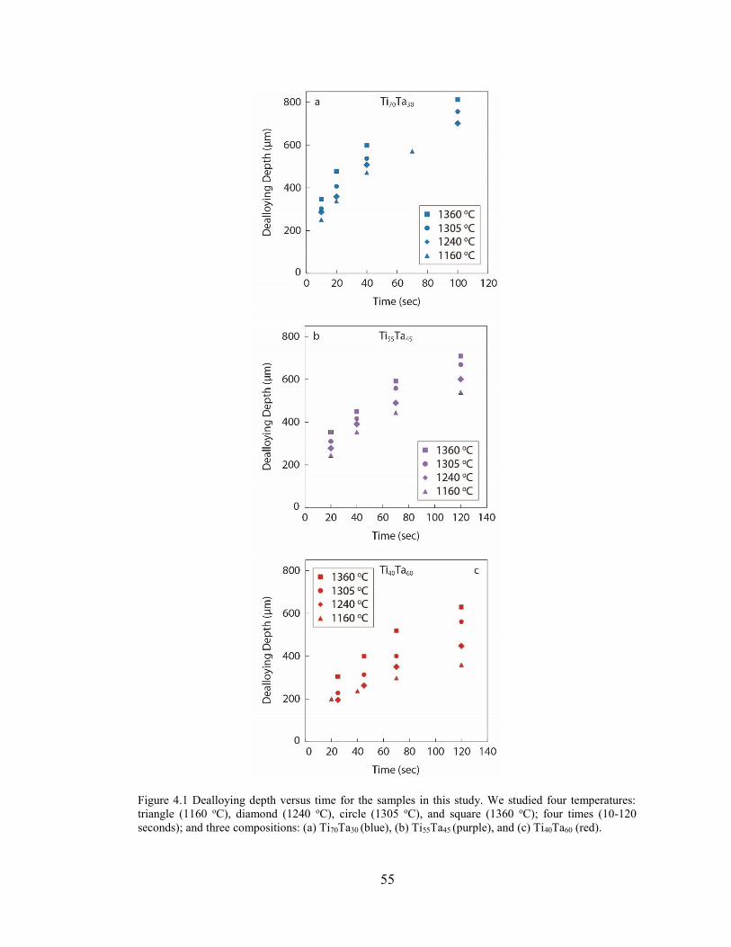
55

Figure 4.1 Dealloying depth versus time for the samples in this study. We studied four temperatures:

triangle (1160 oC), diamond (1240 oC), circle (1305 oC), and square (1360 oC); four times (10-120

seconds); and three compositions: (a) Ti70Ta30 (blue), (b) Ti55Ta45 (purple), and (c) Ti40Ta60 (red).

56

Figure 4.2 Scanning electron microscopy (SEM) micrographs of Ti55Ta45 samples dealloyed in molten

Cu for 20 seconds at four temperatures. The dealloying interface is sharp and flat, and the dealloyed

region has a natural contrast due to the different compositions; the dark phase is Cu and the light phase

is Ta. The top two images were taken at 200x magnification and the bottom two were taken at 270x

magnification, but it can be seen that dealloying depth increases with increasing time.

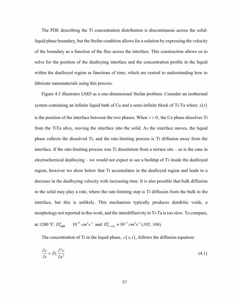
57

The PDE describing the Ti concentration distribution is discontinuous across the solid-

liquid phase boundary, but the Stefan condition allows for a solution by expressing the velocity

of the boundary as a function of the flux across the interface. This construction allows us to

solve for the position of the dealloying interface and the concentration profile in the liquid

within the dealloyed region as functions of time, which are central to understanding how to

fabricate nanomaterials using this process.

Figure 4.3 illustrates LMD as a one-dimensional Stefan problem. Consider an isothermal

system containing an infinite liquid bath of Cu and a semi-infinite block of Ti-Ta where s t

is the position of the interface between the two phases. When 0t , the Cu phase dissolves Ti

from the TiTa alloy, moving the interface into the solid. As the interface moves, the liquid

phase collects the dissolved Ti, and the rate-limiting process is Ti diffusion away from the

interface. If the rate-limiting process was Ti dissolution from a terrace site – as is the case in

electrochemical dealloying – we would not expect to see a buildup of Ti inside the dealloyed

region, however we show below that Ti accumulates in the dealloyed region and leads to a

decrease in the dealloying velocity with increasing time. It is also possible that bulk diffusion

in the solid may play a role, where the rate-limiting step is Ti diffusion from the bulk to the

interface, but this is unlikely. This mechanism typically produces dendritic voids, a

morphology not reported in this work, and the interdiffusivity in Ti-Ta is too slow. To compare,

at 1200 oC 9 2 110S

Ti TaD cm s and 5 2 110L

Ti CuD cm s

(105, 106).

The concentration of Ti in the liquid phase, ,c x t , follows the diffusion equation:

2

2L

c cD

t x

(4.1)

58

where LD is the diffusivity of Ti in liquid Cu. The Stefan condition at the moving boundary,

x s t , is

,Ti Ti

S L L

ds cc c D s t t

dt x

(4.2)

where Ti

Sc is the concentration of Ti in the solid at the interface, and Ti

Lc is the concentration

of Ti in the liquid at the interface.

Figure 4.3. Illustration of liquid metal dealloying. The dealloyed region (dashed lines) is bounded on the

left by molten Cu (orange) and on the right by undealloyed Ti-Ta (gray). The interface between the solid

and the liquid Cu is initially at 0x , and when 0t molten Cu dissolves Ti out of the solid, moving

the interface, s t , towards the right ( t

s t

). The Ta atoms are left behind, reorganizing into a

porous network.

59

An expression for the concentration profile is derived in Appendix B.1 and is given by Eq.

(B.6), repeated here:

,2

Ti TiTiL

L

c c xc x t erf c

erf D t

(4.3)

Here, Tic is the concentration in the Cu bath and λ can be fit experimentally or determined

numerically from the analytical solution derived in Appendix B.2, Eq. (B.10), repeated here:

2Ti Ti

L

Ti Ti

S L

c cerf e

c c

. (4.4)

It is noted in Appendix B.1, but we would like to emphasize that Eq. (4.3) accounts for the

effects of induction heating and the solution given by Eq. (B.4) should be used if the LMD

experiment uses resistive heating. In the case of induction heating we assume that the edge of

the sample will always have the same Ti concentration as the bulk liquid, i.e. 0, Tic x t c

. We introduce this assumption because induction melting induces eddy currents, which add

convection to system outside of the dealloyed region. The degree of convection could be

backed out by immersing samples at different rotation rates, controlling the convection and

measuring the concentration profile (this is similar to a rotating disc electrode setup in

electrochemistry), but that is experimentally challenging and beyond the scope of this work.

The inherent convection caused by induction melting creates a beneficial and serendipitous

steep concentration gradient at the outer geometric surface of the sample; we predict an

increase in the dealloying rate compared to dealloying in a typical resistive-heating furnace.

60

4.4.3 Concentration Profiles

In general, Eq. 3 fits our data well, with one caveat. As shown by example in Figure 4.4,

our data deviates from our model near the original outer surface of our samples, where the raw

data shows a relatively greater concentration of Ti. We believe this deviation is due to

coarsening of the Ta-rich ligaments, and is analogous to post-dealloying coarsening in

electrochemical dealloying where the ligaments enrich in the noble component (9, 107).

During coarsening, Ti inside the ligaments become exposed to the surface through Ta-mediated

surface smoothening and genus-reduction events, and then dissolve into the liquid phase (35).

This surface diffusion process has an approximate 1 4t dependence and has a minor effect on

the dealloying velocity (section 3.4) (35, 37). The Ta-rich ligaments can be considered finite

point sources of Ti, and it can be seen in Figure 4.5 that Eq. (4.3) better fits the concentration

profile at later times when the ligaments near the edge of the sample become depleted in Ti.

Using Eq. (B.5), we performed a least squares fit on the experimental data for 1240 oC for each

composition (Ti70Ta30, Ti55Ta45¸ and Ti40Ta60), and obtained values for the diffusivity (Table

4.1) very close to the literature value (106). The literature value is from a series of experiments

by Shurygin & Shantarin where they measured Ti dissolution in molten Cu across the range

1100-1400 oC using a rotating Ti rod to overcome connective transfer and determine a true

diffusion coefficient for Ti in molten Cu. We excluded the portion where the experimental

curves deviate from the model due to ligament coarsening during the fit, however as shown in

Figure 4.5 this region is quite small for the longer times and is not a significant source of error.

61

Figure 4.4. Comparison of Ti concentration in the Cu phase versus distance away from the dealloying

interface between the experimental data (blue markers) and the analytical model (dashed lines) using the

two different boundary conditions. The analytical model matches well if we assume the Ti concentration

at the edge of the sample is always zero, which is the result of electromagnetic stirring caused by induction

melting. The deviation between the model and the experimental data at distances far from the interface

is due to ligament coarsening, which adds extra Ti to the Cu bath.

62

Figure 4.5. Ti Concentration versus distance away from the dealloying interface for Ti70Ta30 at 1240 oC.

Experimental data (blue markers) compared with Eq. (B.5) at different times: (a) 10 seconds, (b) 20

seconds, (c) 40 seconds, and (d) 70 seconds. Eq. (B.5) was simultaneously fit across all times yielding

5 2 11240 6.5 10LD C cm s , agreeing well with the literature value

5 2 1(1240 ) 7.0 10Ti CuD C cm s

.

63

4.4.4 Dealloying Depth

An expression for the dealloying depth is derived in Appendix B.2, Eq. (B.11), repeated

here:

24 Ls t D t . (4.5)

We used Eq. (4.4) and the experimentally measured concentrations to determine λ for each

composition, and backed-out the diffusivity and activation energy for each composition by

collapsing the data from each temperature onto the curve 24s t t , where Lt t D ,

0 expL a BD D E k T , aE is the activation energy for Ti diffusion in molten Cu, and T is

the temperature of the reaction. The values determined from this fit are listed in Table 4.1, and

activation barriers for all compositions less than Ta60 agree well with literature values.

However, the fit 0D values differ by two orders of magnitude from the literature value. We

suggest this discrepancy is due to the additional Ti added to the bath from ligament coarsening:

i.e., extra Ti at the edge of the sample reduces the driving force for Ti diffusion away from the

dealloying front, and a more rigorous form of Eq. (4.5) would include a second, albeit minor,

term with a 1 4t dependence to reflect this effect. It is also possible that the tortuosity of the

dealloyed structure may interfere with Ti diffusion, increasing the diffusion path length from

the dealloying interface to the edge of the sample. Thus, we hypothesize relaxing the form of

Eq. (4.5) to

24n

Ls t D t (4.6)

and allow the exponent n to be determined from the experimental fit. Figure 4.6 is a plot of

the collapsed data versus t and it can be seen that each data set has close groupings.

64

The values for the exponent were found to be close to 0.5n , with70 30

0.38Ti Tan ,

55 450.41Ti Tan , and

40 600.45Ti Tan . It is reasonable that the exponent for the Ti70Ta30 data set is

lower than the Ti55Ta45 and Ti40Ta60 data sets because there will be more residual Ti in the Ta

ligaments, which will lead to a larger effect from coarsening. Consistent with this idea, we see

the exponent approach 0.5n as we increase the Ta concentration. The values of 0D for all

compositions using Eq. (6) to fit s t are within an order of magnitude of the literature value

and agree much better than the fit using Eq. (4.5). The activation energies for Ti70Ta30, Ti55Ta45

were found to be 0.67 eV and 0.69 eV , respectively, which is very close to the literature value

0.715Ti CuE eV . Interestingly, the value for Ti40Ta60 , 1.29aE eV , was much higher than

samples at lower Ta composition, suggesting a different mechanism became the rate limiting

step. This could either be a switch to attachment/detachment-limited regime such as seen in

electrochemical dealloying, or an effect of the morphology of the dealloyed structure, which

will be addressed in section 3.6.2.

Table 4.1 Kinetic parameters determined for the compositions in this study.

Composition 2 1(1240 )LD C cm s n 2 1

0 ( )D cm s ( )aE eV

literature value 57.0 10 - 0.5 21.7 10 0.715

Ti70Ta30 56.5 10 0.99 0.38 4,*4.6 10 2,**3.4 10

*0.45 **0.67

Ti55Ta45 53.3 10 0.915 0.41 4,*8.2 10 3,**6.5 10

*0.57 **0.69

Ti40Ta60 54.8 10 0.88 0.45 2,*4.8 10 1,**1.2 10

*1.17 **1.29

* indicates parameter fit using Eq. (4.5) **indicates parameter fit using Eq. (4.6)

65

Our final comment on the dealloying depth is the effect of grain boundaries, which can

significantly alter the kinetics. Figure 4.7 is a cross-section of a Ti65Ta35 sample (dealloying

depth data not included in this work due to the ingot’s small grain size) dealloyed at 1160 oC

for 120 seconds. The dealloying interface is much rougher than the ones Figure 4.2, making it

difficult to measure an accurate dealloying depth. We speculate that this is the result of

different grains dealloying at different rates, but more importantly from grainboundaries

themselves.

We observed grainboundaries are always dissolved first during LMD, replacing the solid-

solid interface between adjacent grains with a solid-liquid-solid interface; at later times the

Figure 4.6 Collapsed dealloying depth versus scaled time 0 exp a Bt t D E k T for Ti40Ta60 (red),

Ti55Ta45 (purple), and Ti70Ta30 (blue). The symbol shape corresponds to the experimental temperature:

triangle (1160 oC), diamond (1240 oC), circle (1305 oC), and square (1360 oC). Dashed lines: fits to the

data using the relationship 24n

Ls t D t . The values of ,0D ,

aE , and n were determined for each

data set and are listed in Table 4.1.

66

regions between grains fully detach and a thick Ta-rich region appears (Figure 4.7). It is not

accurate to call these regions grain boundaries because the solid-solid interface is destroyed

during dealloying, but we will use this name out of convenience. Dealloying is slower in

regions where grainboundaries are perpendicular to the dealloying direction, and we think it is

reasonable to conclude the boundaries impede Ti diffusing away from the dealloying interface.

For this reason we made sure that all of the starting alloys in this study were sufficiently

annealed, and most samples had an average grain size of ~500 um. We caution future work to

be aware that boundaries can alter the kinetics, and it is desirable to have as large grains as

possible to dealloy to large depths.

Figure 4.7. Effect of grain boundaries on dealloying kinetics. Ti65Ta35 (dealloyed depth data not included

in this work) sample dealloyed at 1160 oC for 120 seconds. The grains in this structure are small, causing

an inhomogenous dealloying interface, contrasting with Figure 4.2. It can also been seen that the

boundaries dissolve faster than the interior of the grains.

67

4.4.5 Parting Limit

We will briefly discuss the parting limit in liquid metal dealloying, which has been

extensively studied in electrochemical dealloying (18, 23, 108). This concept was introduced

in section 1.3.1, but it is worth reiterating that the parting limit, or percolation threshold cp , is

the critical alloy composition (defined in the percentage of the dissolving component)

necessary for a structure to fully dealloy. For dealloying it is important to introduce the concept

of high-density percolation, cp m , which denotes that a percolation path exists composed of

atoms [of the dissolving species] with at least m neighbors. We expect The Ti-Ta alloy system

to have a higher percolation threshold than fcc dealloying systems such as Ag-Au because the

bcc lattice has fewer nearest neighbors. This idea is corroborated by 1 24.5bcc

cp , whereas

1 19fcc

cp at.%.

In this study we did not characterize a parting limit in detail; however, out data suggests it

likely sits around 40 at.% Ti. We attempted to dealloy Ti30Ta70 and Ti20Ta80 samples but did

not observe any significant dissolution. Samples from both alloys were immersed into molten

Cu for several minutes, and we only saw small channels of Cu near the surface of the sample

which were no wider than 500 nm and no longer than tens of microns. Previous work in

electrochemical dealloying has demonstrated that surface dealloying can always occur due to

low coordination at the surface, but this does not imply the sample will fully dealloy.

Analogously, liquid metal embrittlement can occur in systems with no dissolving component

such as Al embrittlement by Ga. We were able to dealloy Ti40Ta60, however the activation

barrier for this composition was almost twice that of the activation barrier for Ti55Ta45 and

Ti70Ta30; it is possible 40 at.% Ti is just above the percolation threshold. This low parting limit

is surprising but other fcc dealloying systems such as Al-Cu and Zn-Cu have thresholds close

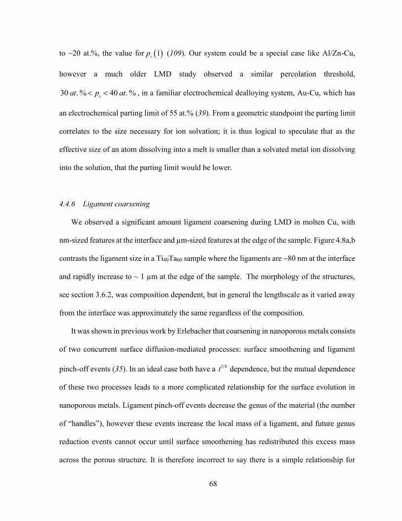
68

to ~20 at.%, the value for 1cp (109). Our system could be a special case like Al/Zn-Cu,

however a much older LMD study observed a similar percolation threshold,

30 . % 40 . %cat p at , in a familiar electrochemical dealloying system, Au-Cu, which has

an electrochemical parting limit of 55 at.% (39). From a geometric standpoint the parting limit

correlates to the size necessary for ion solvation; it is thus logical to speculate that as the

effective size of an atom dissolving into a melt is smaller than a solvated metal ion dissolving

into the solution, that the parting limit would be lower.

4.4.6 Ligament coarsening

We observed a significant amount ligament coarsening during LMD in molten Cu, with

nm-sized features at the interface and µm-sized features at the edge of the sample. Figure 4.8a,b

contrasts the ligament size in a Ti40Ta60 sample where the ligaments are ~80 nm at the interface

and rapidly increase to ~ 1 µm at the edge of the sample. The morphology of the structures,

see section 3.6.2, was composition dependent, but in general the lengthscale as it varied away

from the interface was approximately the same regardless of the composition.

It was shown in previous work by Erlebacher that coarsening in nanoporous metals consists

of two concurrent surface diffusion-mediated processes: surface smoothening and ligament

pinch-off events (35). In an ideal case both have a 1 4t dependence, but the mutual dependence

of these two processes leads to a more complicated relationship for the surface evolution in

nanoporous metals. Ligament pinch-off events decrease the genus of the material (the number

of “handles”), however these events increase the local mass of a ligament, and future genus

reduction events cannot occur until surface smoothening has redistributed this excess mass

across the porous structure. It is therefore incorrect to say there is a simple relationship for

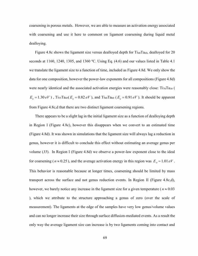
69

coarsening in porous metals. However, we are able to measure an activation energy associated

with coarsening and use it here to comment on ligament coarsening during liquid metal

dealloying.

Figure 4.8c shows the ligament size versus dealloyed depth for Ti40Ta60, dealloyed for 20

seconds at 1160, 1240, 1305, and 1360 oC. Using Eq. (4.6) and our values listed in Table 4.1

we translate the ligament size to a function of time, included as Figure 4.8d. We only show the

data for one composition, however the power-law exponents for all compositions (Figure 4.8d)

were nearly identical and the associated activation energies were reasonably close: Ti70Ta30 (

1.30aE eV ) , Ti55Ta45( 0.82aE eV ), and Ti40Ta60 ( 0.91aE eV ). It should be apparent

from Figure 4.8c,d that there are two distinct ligament coarsening regions.

There appears to be a slight lag in the initial ligament size as a function of dealloying depth

in Region I (Figure 4.8c), however this disappears when we convert to an estimated time

(Figure 4.8d). It was shown in simulations that the ligament size will always lag a reduction in

genus, however it is difficult to conclude this effect without estimating an average genus per

volume (35). In Region I (Figure 4.8d) we observe a power-law exponent close to the ideal

for coarsening ( 0.25n ), and the average activation energy in this region was 1.01AE eV .

This behavior is reasonable because at longer times, coarsening should be limited by mass

transport across the surface and not genus reduction events. In Region II (Figure 4.8c,d),

however, we barely notice any increase in the ligament size for a given temperature ( 0.03n

), which we attribute to the structure approaching a genus of zero (over the scale of

measurement). The ligaments at the edge of the samples have very low genus/volume values

and can no longer increase their size through surface diffusion-mediated events. As a result the

only way the average ligament size can increase is by two ligaments coming into contact and

70

fusing together. This appears to be a very slow process, and the ligament size does not increase

significantly in Region II.

4.4.7 Morphology

In Chapter 3 we noted that the morphology of structures fabricated using liquid metal

dealloying can be dramatically different depending on parent alloy composition. We observed

a morphology transition from Ta droplets to a connected, porous Ta network as the parent alloy

composition changed from Ti95Ta5 to Ti65Ta35. In this current study we are only examining

connected structures, and report subtle changes in the morphology. Specifically we see an

increase in the connectivity of the structures as we increase from 30-60 at.% Ta, which in turn

affected the stability of the Ta network at longer times (Figure 4.9).

We observed good mechanical integrity when the Ta concentration was greater than ~30

at.%, owing to the connectivity in the porous network, which is a major reason why this work

focuses on Ta-rich alloys. Samples with lower Ta concentrations were mechanically stable for

short immersion times (less than 10 seconds), but fell apart during longer immersions (greater

than 20 seconds). Only samples with at least 30 at.% Ta were robust enough to hold together

during long immersion experiments (up to 120 seconds). Ligament pinch-off mediated

coarsening decreases the connectivity of the porous structure with increasing time, and

eventually ruins the mechanical integrity of the sample. Not only did the connectivity depend

on time but also on the Ta composition. For comparison, Figure 4.9 shows the connectivity of

the ligaments change at the edge of the sample from disconnected blobs in the Ti70Ta30 sample

to a highly connected structure in the Ti40Ta60 sample. This effect is quite significant in Cu

71

baths, however it should be less obvious in lower-melting point baths where the ligaments do

not coarsen significantly past their formation size.

It was mentioned in section 3.4 that the activation energy for Ti diffusion in molten Cu for

the Ti40Ta60 composition was quite high, almost twice that for Ti55Ta45 and Ti70Ta30. It is

possible that the high connectivity at the interface significantly limits the diffusion path for Ti

atoms out of the dealloyed structure, and the limiting mechanism becomes a pinch-off event to

allow the Ti atom to “escape” this highly tortuous region. This activation energy was very

similar to the activation energy for coarsening in section 3.6.1, however it is very difficult to

deconvolute pinch-off events from surface smoothening events.

Figure 4.8. Ligament coarsening during LMD using Ti40Ta60 as an example. (a) SEM micrograph of the

dealloying interface (bottom of the image) showing ligaments ~80 nm at the interface. (b) SEM

micrograph of the edge of the sample (bottom of the image) showing ~1.5 µm ligaments at the edge of

the sample. (c) Ligament size versus distance from interface. (d) Ligament size versus estimated time.

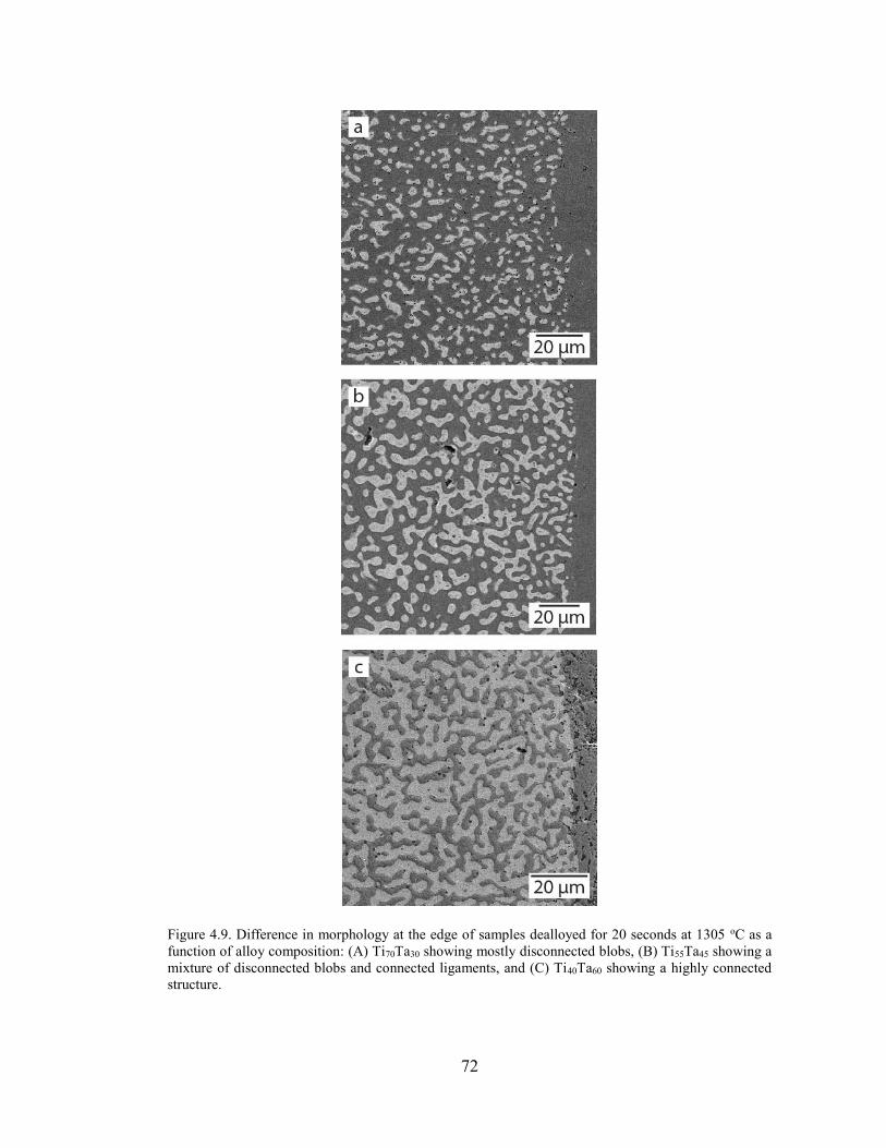
72

Figure 4.9. Difference in morphology at the edge of samples dealloyed for 20 seconds at 1305 oC as a

function of alloy composition: (A) Ti70Ta30 showing mostly disconnected blobs, (B) Ti55Ta45 showing a

mixture of disconnected blobs and connected ligaments, and (C) Ti40Ta60 showing a highly connected

structure.

73

4.4.8 Homologous Temperature Effects

We demonstrated in Chapter 3 that by adding Ag and Bi to molten Cu we can fabricate

molten baths with lower melting points and thus refine the ligament size of the porous structure.

What we left out of that discussion was that each sample was dealloyed for a significant time,

and the samples were only dealloyed to a depth of 150 m .

The only drawback to making alloy baths is maintaining a high solubility of the dissolving

component. Across this temperature range, Bi( ) and Ag( ) have at most 4 and 2 at.% Ti

solubility, respectively, although it is unclear how Cu affects the solubility. Referring back to

Eq. (B.10) and Eq. (4.6) the dealloying rate is highly dependent on the solubility in the liquid

phase as well as the concentration in the liquid bath. As a result, the dealloying rate becomes

very sensitive to the size of the bath, and large quantities are needed to dealloy thin samples.

Future work will need to explore balancing the addition of components to the liquid bath to

suppress coarsening without killing the dealloying rate.

4.5 Summary and Conclusions

We examined the kinetics of liquid metal dealloying by varying the parent alloy

composition, dealloying temperature, and dealloying time. The values measured for the

diffusivity and activation energy confirm that the rate-limiting step in the dealloying process

is Ti diffusion away from the dealloying interface and out of the dealloyed structure, however

a second mechanism may become dominant when the alloy composition is close to the parting

limit. Serendipitously, induction heating adds convection to the system, and we predict an

increase in the dealloying rate compared to dealloying using resistive heating. The dealloying

depth has a power-law relationship with an exponent close to 0.5n , with a deviation

74

attributed to ligament coarsening adding extra Ti to the Cu bath. Ligament coarsening is very

fast at this temperature, increasing from 80 nm to 1 µm in just 10 seconds. We observe two

distinct power-law exponents during coarsening owing to ligament pinch-off and surface

smoothening events occurring simultaneously. To stymie coarsening we performed LMD

experiments in lower-melting point baths, however the low Ti solubility in these baths made it

difficult to dealloy to large depths (of order 1 mm). There is a challenge in LMD to fabricate

bulk structures with nm-sized ligaments, and future work will need to address this issue.

Nevertheless, this chapter is meant to develop a framework for liquid metal dealloying, and

lays the groundwork for future research in this field.

75

Chapter 5 Mechanical Properties of Refractory-based

Nanocomposites

5.1 Summary

In this chapter we explore the mechanical properties of nanocomposites fabricated using

liquid metal dealloying (LMD). The compressive strength of metal single-crystalline

micropillars has been shown to increase with decreasing diameter, but translating this size-

dependent strength enhancement to bulk materials has been a challenge; joining of

macroscopic materials is inherently challenging and it would be costly to create nano-truss

materials using a similar technique (110). Recent efforts have produced ~1 mm3 lattice

materials 20 nm features, however this requires a complex combination of lithographic laser

writing and decomposition of polymers (110–112). Here we utilize LMD as a potential

fabrication route for bulk nanostructured materials. The LMD process results in

nanocomposites with two distinct phases: a single-crystalline refractory metal network

embedded in a Cu-rich matrix. The properties of each phase has the potential to be tailored,

and the nanocomposites demonstrate an increase in yield strength that scales with network

feature size.

76

5.2 Background

It is a well-established principle in the mechanics of crystalline materials that smaller

microstructural features yield stronger materials. There are numerous manifestations of this

effect, including variations in grain size, metallic film thickness, indentation depth, nanowire

and micropillar diameter, and ligament diameter in nanoporous metals. The central idea is that

dislocation activity is different in reduced volumes where interactions with free surfaces can

lead to dislocation starvation, source truncation, or pileup (113). An important point of

distinction is that these mechanisms can be divided into extrinsic factors (e.g. external crystal

dimension) and intrinsic factors (e.g. precipitate size) (114). Modern physical metallurgy is

founded on designing materials with precisely controlled intrinsic microstructures, e.g.

solution and precipitation hardened materials, however extrinsic effects have the potential to

play an important role because small-volume materials (e.g. metallic whiskers) approach the

theoretical strength of a material (113, 115, 116). In order to develop new materials with

extrinsic “microstructures” recent academic efforts have focused on assembling bulk structures

out of nano-scale materials (111, 112).

Nanoporous metals (np-metals) are an interesting class of materials because they are a self-

assembled structure and 3~ 1 mm of material can be fabricated easily in a laboratory setting

(43–45). Electrochemical dealloying is quite slow, with an etch rate of ~ 1 secnm , however

we showed in the previous chapter that liquid metal dealloying is capable of etching at a rate

of ~ 15 secm . Interestingly, the limiting factor in dealloying is the depth of a component,

and large volumes could be produced providing the surface area of the component is much

larger than its thickness. However, in full disclosure the largest np-metal fabricated to date is

77

3~ 1 cm and there are significant challenges in scaling up the material which will only be

addressed when these materials have found an industrial application (1, 45).

Despite only being used in laboratory setting, np-metals have a high degree of tunability,

with the most obvious parameter being the ligament size. To illustrate this point, the as-

fabricated ligament size of np-Au is ~10 nm, however the material can be coarsened to ~10

µm by heating in a furnace at 650 oC for 10 minutes while retaining a self-similar structure

(13, 35, 82). As discussed in the previous chapter the ligament size follows a 1 4t relationship,

and it is expected that larger ligament sizes ( 100 m ) could take days to fabricate.

Additionally, the starting alloy composition can be altered, resulting in different densities as

well as altering the final ligament composition. More radical changes have involved multiple-

step dealloying to produce bimodal hierarchical porosity, or adding ternary alloying

components to alter the surface chemistry.

5.2.1 Ligament Size Effect in the Yield Strength of Nanoporous Metals

The purpose of this section is to discuss the mechanical properties of np-metals reported in

the literature. Using literature data from 15 different publications in Chapter 1, we will address

the current limitations and provide an outlook on the future of these materials.

The wealth of the work on the size-dependence of the yield strength in np-metals has been

performed on np-Au, however, the scaling laws are expected to be the same for all bicontinuous

np-metals (46–49, 51, 53–55, 57, 61). The first important point to address is why yield strength

values reported for np-Au have reduced properties compared to bulk Au. Examining Figure

1.5 reveals that only one research group measured yield strengths above the value for bulk Au

(~100 MPa) (117, 118). Np-metals have been commonly compared to metallic foams, which

78

have reduced properties compared to their bulk counterparts. Following the Gibson-Ashby

(GA) relation for bending dominant behavior, 3 2

foam

y , where is the relative density.

The GA relation was derived for low-density foams with high aspect ratios (thickness/length

ratio), however np-metals have low aspect ratios where 1t l (66). Nevertheless, we should

be able to construct a purely empirical relationship for the yield strength of np-metals as a

function of the relative density. Before we can determine the yield strength dependence on

relative density we need to establish what fully-dense material we can compare np-metals to.

There are many possibilities – Au micropillars, nanocrystalline Au, Au nanowires, and Au thin

films – but we will start be examining the size-dependent behavior of np-Au in literature.

Figure 5.1 shows a plot of three different data sets of np-Au: two are hardness data of two

different densities compiled from References (46, 56, 66) , and one data set is compression

data of a different density from Reference (66). Care was taken to use only relative densities

* where there was a significant amount of data, and data sets with relative densities greater

than 0.02 were not considered to be the same density. There is a disagreement in the field

regarding conversion of hardness to a yield strength for nanoporous metals, which we will

discuss below, but we ignore this for now because the conversion uses a scalar and we are only

interested in the power-law exponent m from the data.

It is readily apparent that there is a different power-law exponent m associated with each

relative density * , even though in principle the exponent should be density-independent.

Nevertheless, the three data sets display similar scaling, and averaging them yields a power-

law exponent 0.59m , which is in close agreement with the power-law exponent reported

for single crystal Au micropillars ( 0.61m ) by Volkert & Lilleodden (119) and the general

power-law for micropillars ( 0.66m ) reported by Dou & Derby (72). There is an obvious

79

error in our adaption of the hardness/yield data from the References (since they don’t fall on

each other), but there is also a seldom-reported error inherently in nanoporous metal data sets,

namely, the ligaments in nanoporous metals are three-dimensional shapes and the standard

deviation of an average ligament size and length can easily be 20 30% within each data

set. This variation is a direct result of coarsening in porous metals. It should also be expected

that the larger ligaments are weaker and play a significant role in the macroscopic mechanical

behavior. This idea could be tested by statistically analyzing what percentage of large

ligaments would be necessary to induce premature failure.

Regardless, it is important to emphasize that the average value of the power-law is

generally larger than the Hall-Petch exponent 0.5m and smaller than thin films where the

strength scales with the inverse of the film thickness, which is to be expected because

nanoporous metals are single crystalline within each grain and are not confined materials. We

do not believe it is reasonable to compare np-metals to dislocation-starved structures because

TEM studies by Balk & Minor have shown that these materials, as formed, have dislocations

present which are activated during deformation and do not immediately run out of the sample

as shown in in situ TEM studies on 200 nm Ni nanopillars (60, 113, 120). An interesting study

on defect-free Mo micropillars showed that there was no increase in strength with decreasing

feature size and the reported stress for every diameter was approximately the theoretical yield

strength (121, 122); this same work also reported that dislocation starvation did not occur in

any of these structures after yielding. It is apparent that there are disagreements in the field of

nanomechanics as to the underlying material behavior at the nanoscale and research is ongoing

to fully explain experimental observations. In any case, we have shown that np-metals show

size-dependent behavior with a power-law similar to that of micro- and nano-pillar materials.

80

As mentioned, Figure 5.1 includes hardness data, which is not an issue when considering

size-dependent strengthening, but becomes relevant when comparing the data to yield strength

values measured by compression and tension testing. For dense metals the hardness-to-yield

strength conversion relationship is typically 3 yH , where H is the Vickers hardness, but

metallic foams with relative densities below 0.3 are fully compressible materials and all

deformation is transferred into densification of the ligaments, resulting in the relationship

yH (46, 51, 56). There have been discrepancies between hardness and yield strength data

in nanoporous metals deriving from conflicting observations of transverse plastic strain, which

Figure 5.1. Hardness and yield strength data versus ligament diameter for three different densities from

References (46, 56, 66). It is apparent that the strength increases with decreasing feature size, with a

power-law exponent similar to that in single crystal micropillars.

81

is used to determine the plastic Poisson’s ratio and ultimately the true H vs. y relationship.

Compression testing by Volkert et al. and Briot & Balk (57, 66) yielded a plastic Poisson’s

ratio of ~ 0.2 for materials with 0.33 and * 0.35 , which yields the relation

2.65 yH . In a different study, Jin and coworkers (56) determined a plastic Poisson’s ratio

of ~ 0.0 for materials with 0.26 and 0.275 , however there was a limited number of

samples tested so it is difficult to confirm this result. Despite observing no plastic strain, the

authors in the latter work agreed that the hardness values matched well with their compression

values when they used the conversion 3 yH . It is difficult to make a conclusion regarding

the plastic Poisson’s ratio because neither group tested the same relative density.

Simulation work has also examined the effect of a plastic Poisson’s ratio: finite element

modeling by Huber et al. (64) demonstrated the plastic transverse strain went to zero with

increasing disorder/randomization in the ligaments. A set of molecular dynamics experiments

by Farkas et al. (62) demonstrated a plastic Poisson’s ratio close to zero for samples tested in

compression, and a large plastic Poisson’s ratio ( 0.45 0.6 ) for samples tested in tension; and

a recent MD study by Bao-nam et al. (63) showed no transverse strain in compression testing.

Unfortunately, these MD simulations looked at materials with relative densities 0.3 and

are not directly applicable to experimental differences. A third set of MD simulations by Sun

et al. (71) looked at different densities in tension but did not comment on transverse strain.

Despite the differences between these research groups, the hardness data matches well with

the compression and tension data if a scalar prefactor 2.65 or 3 is used. Thus, we think it is

reasonable to conclude that yH is likely most appropriate. For the following discussion

we used a prefactor of 2.65.

82

The above discussion suggests that the function form of the size-dependent yield strength

of np-Au is similar to that of micropillars. If we can make such an analogy, it follows that we

can treat Au micropillars as a fully-dense material ( 1 ) and solve for the Gibson-Ashby

(GA) parameters C and n by collapsing the three data sets in Figure 5.1 onto the Au-

micropillar data; this exercise yields average values of 1.38C and 2.71n . These are

similar to the values reported by Briot & Balk (66), where 1.939C and 2.618n , and

significantly different from the values of C and n expected in bending-dominant behavior

underpinning Equations (1.1) and (1.2). It was pointed out by Liu & Antoniou (123) that the

GA relation is true for long-cell walls, but nanoporous metals have short ligaments with low

aspect ratios and are expected to behave differently. Unfortunately these empirically derived

constants do not reveal the underpinning deformation mechanism(s) of nanoporous metals, and

in situ experiments will be necessary to conclude their true behavior.

The goal of determining the GA parameters is to negate the effect of the relative density to

compare size-dependent strengthening for a variety of nanoporous materials using the

relationship n

foam bulk

y yC

. The data in Table A.1 represents foam

y , and we can back

out bulk

y using the values of C and n determined above. Figure 5.2a shows the bulk yield

strength versus ligament size we would expect if these materials were fully dense. The dashed

line corresponds to a fit using the data from Au micro- and nanopillars (119), and appears as

an average for the corrected data. Finally, Figure 5.2b is the bulk yield strength, material-

normalized data for all mechanical data on nanoporous metals, including values of nanoporous

Ag, Cu, Pd, and Ti. Unfortunately there is still significant deviation, an order of magnitude,

reflecting how difficult it is to fabricate consistent samples between research groups.

83

Figure 5.2. Corrected and normalized yield strength data for np-Au and all nanoporous metals.

84

5.2.2 Nanoporous Metal-Based Composites for Enhanced Ductility

The previous sections have shown that nanoporous metals show size-dependent

strengthening, however their low-densities diminish the effects of this property. Additionally,

as mentioned in Chapter 1, these materials are macroscopically brittle. Clearly there is a need

to develop strategies to improve the mechanical integrity of these materials in order for them

to find real-world application. Researchers have developed several different

strengthening/toughening strategies to enhance the mechanical properties of dealloyed

nanoporous metals. These strategies include creating core-shell structures, refining the pore

size, and filling the void space with an electrolyte or polymer (43–45, 59, 76, 124, 125).

The first observation of altering the properties in np-Au was reported by Senior & Newman

(125), where they observed that np-Au became very flexible when the pores were filled with

DI water. This work was briefly explored in (126), however, the material had a yield strength

and elastic modulus lower than np-Au because it was a metal-water composite. Abdolrahim et

al. (59) explored the idea of coating the ligaments of np-Au with Ni, and observed a five-fold

increase in the strength of the material compared to np-Au. The Ni phase underwent significant

twinning, accommodating plasticity in the material and may have allowed for work hardening

in the Au phase, leading to a macroscopically ductile material. Similar strengthening has been

observed in coated micropillars and confirm that the performance increase is not the result of

a skin-thickness effect. More recent strengthening strategies to improve the mechanical

properties of nanoporous metals have involved infiltrating the porous phase with a secondary

material. Wang & Weissmuller (43, 44) examined metal-polymer composites, and saw

significant increases in ductility and strength, even achieving 10% strain in tension. These

composites are fully dense materials and are expected to undergo different modes of

85

deformation, similar to those observed in (59, 127, 128), and Gibson-Ashby relations are not

applicable in these materials. We will explore this in the following sections, but a size-

dependent rule of mixtures model may be more appropriate.

In this chapter we expand on the idea of filling the pores of nanoporous metals, using the

LMD process to create high-strength composite materials by allowing the dealloying medium

to solidify inside the pores. The composite materials we fabricated show a ten-fold increase in

yield strength when we decrease the feature sizes from 10 µm ( ~ 250 MPa ) to 70 nm (

~ 2.5 GPa ), while still retaining plastic behavior. This is the first report of metal-metal

bicontinuous nanocomposite materials and the first assessment of their mechanical behavior.


5.3.1 Ingot and Bath Preparation

50g Ti65Ta35, Ti20Ta80, and Ti75W25 alloy buttons were prepared by the Materials

Preparation Center at Ames Laboratory. The raw materials used were Ti (99.9 wt.%), Ta (99.9

wt.%), and W (99.9 wt.%). The Ti-W alloy has an extremely high melting point, and the as-

received button was not fully dense; the button was remelted by Arcast, Inc. using a water-

cooled cold crucible. Approximately 1 cm3 ingots for LMD were cut using wire electrical

discharge machining (EDM), and then annealed via induction melting in a ultra-high vacuum

(10-8 torr) environment at ~ 1500 oC for 72 hours.

Metal baths for the LMD process were prepared by premelting ~20 g ingots of Cu, and

Cu32Ag68. Commercially pure Cu (99.99 wt .%), and Ag (99.99 wt. %) pellets were melted in

a graphite crucible under flowing Ar. Control samples of Cu90Ti10, Cu75Ti25, Cu65Ti35, and

86

Cu50Ti50 were fabricated in-house using induction melting using Ti (99.98 wt.%) and Cu used

above.

5.3.2 Composite Fabrication

Composites were fabricated using an LMD process by immersing individual Ti-X ingots

into a 20 g bath of molten Cu/Ag in an ultra-high purity alumina crucible cast in-house using

materials from Cotronics Corp. Induction melting was used to heat the samples under flowing

Ar (99.99%), and the LMD process was run for a set time. Samples details are included in

Table 5.4.

Table 5.1. Mechanical data from microtensile tests.

Sample Ligament Size

(µm)

Immersion Time

(sec)

Number of

Tests

Type of Test

Ta/Cu 10.56 0.31 20 4 compression




Ta/CuAg 0.500 0.020 20 20 nanoindentation



W/Cu 0.656 0.107 20 4 compression

W/Cu 1.154 0.200 15 4 compression

W/Cu 1.500 0.050 15 10 microindentation





87

We cut, polished and imaged cross sections to ensure full Cu penetration into the Ti-X ingots

and that the nanocomposites had a uniform ligament size. Nanocomposite samples were

mounted in Struers PolyFast conductive epoxy, and underwent: grinding steps of 400 grit, 600

grit; diamond polishing steps of 9 µm, 3 µm, 1 µm; and a final polishing step of .05 µm.

Composites were characterized using a JEOL scanning electron microscope (SEM) and ImageJ

was used to measure dealloying depth and average ligament sizes. EDS was used to determine

the composition of each phase as a function of depth. Average ligament sizes were determined

by drawing lines across SEM images in ImageJ and measuring ligaments diameters along the

line. At least 50 ligaments were measured from multiple images. We did not quantify the grain

size in the Cu phase or the volume fraction and size of the CuTi precipitates although they are

expected to play an important role in the mechanical properties. Compositions of the Ta and

Cu phases in the composites were measured using energy-dispersive X-ray spectroscopy

(EDS). A summary of the compositional data can be found in Table 5.2.

Table 5.2. Compositional data for Ta/Cu and Ta/CuAg composites.

Material ( .%)Ta at ( .%)Cu at ( .%)Ti at ( .%)Ag at

Ta phase (3,5.2 µm) 80 5 0 20 5 0

Cu phase (3,5.2 µm) 0 75 8 25 8 0

Ta phase (7.7,10.6 µm) 80 5 0 20 5 0

Cu phase (7.7,10.6 µm) 0 90 3 10 3 0

Ta phase (70, 117, 500 nm) 77 10 0 23 10 0

CuAg phase (70, 117, 500 nm) 0 35 2 59 2 6 2

88

5.3.3 Mechanical Testing

Microtensile testing was performed at a strain rate of 42 10 using a 445 N load cell

with a resolution of 0.426 N, and strain was measured using a digital image correlation method

reported in previous works (129, 130). The cross-sectional area was determined from five SEM

measurements per sample with a standard deviation of 3 % , which corresponds to a stress

variation of 8 MPa. Compression testing was performed at a strain rate of 32 10 using a

20 45kN N load cell, and strain was measured using digital image correlation.

Compression sample dimensions were measured using Mitutoyo digital calipers, and the total

error in stress measurement was 16.9 MPa. Details of the stress-strain curves and digital

image correlation for strain estimates are included in Appendix C.1.

Nanoindentation testing was performed using a Nanomechanics iNano indenter with a

Berkovich tip. A continuous stiffness measurement technique was used and samples were

indented at a constant strain rate of 10.2 s up to a depth of 500 nm, and values were averaged

over the depth range 200–500 nm.

5.3.4 W/Cu TEM and APT Preparation

W/Cu nanocomposite specimens were prepared for Transmission Electron Microscopy

(TEM) and atom problem tomography (APT) by Eric Xu and Mingwei Chen at Tohoku

University, Sendai, Japan.

Thin foils for scanning transmission electron microscopy (STEM) observations were

prepared by ion milling at the ion energy of 2 kV and an incident angle of ±6. The TEM

specimens were cooled by liquid N2 during ion milling. Sharp tip specimens for atom probe

tomography (APT) were made by electrochemical micro-polishing and followed by focused

89

ion beam milling to reduce the size of the tips down to a few hundred of nanometers (JIB-

4601F, JEOL). The finished tip profiles were examined by scanning electron microscopy

(SEM) for APT reconstruction. The data acquisition was performed using a local electrode

atom probe (LEAP 4000HR) equipped with an energy compensated reflectron, by which the

mass resolution can be greatly improved. The APT acquisition temperature was set at 50 K,

and the pulse frequency and pulse fraction were 200 kHz and 20%, respectively. The

CAMECA Integrated Visualization and Analysis Software (IVAS 3.6.6) package was used for

data processing and three-dimensional (3-D) atomic reconstruction.

The STEM observations were conducted on a JEOL JEM-2100F instrument equipped with

double spherical aberration correctors for probe forming and image forming lenses. High-angle

annular dark-field (HAADF) STEM images were taken using an annular-type detector with a

collection angle ranging from 100 to 267 mrad, while bright-field (BF) STEM images were

simultaneously recorded using a STEM BF detector. Chemical analyses were carried out by

means of electron energy loss spectroscopy (EELS) and energy dispersive X-ray spectroscopy

(EDX). EELS and EDX elemental mapping and spectra were acquired using a Gatan GIF

Tridiem and JEOL JED-2300T, respectively.

90


5.4.1 Tantalum-based composites

5.4.1.1 Compression and Hardness Testing

Figure 5.3 displays bulk, metal-metal composite samples fabricated by our own variation

of the LMD process. In this figure we show ~1 cm3 Ta/Cu material fabricated from a TiTa

starting material with ~500 µm grains. Figure 5.4 illustrates the features of this bicontinuous

composite: The new material is polycrystalline, consisting of individual, single-crystal bcc

refractory micropillar networks (the “dealloyed phase”), and a rapidly solidified Cu phase (the

“matrix phase"), containing Cu-Ti intermetallic precipitates.

Figure 5.3. Bulk nanocomposites made by liquid metal dealloying. (A) Examples of as-made Ta-Cu

nanocomposites; ~1 cm3 ingot (left), compression testing sample (center), microtensile sample (right).

91

Figure 5.5a shows graphs of engineering stress versus engineering strain from compression

tests on macroscale samples (~5-7 mm3) at a strain rate of 3 12 10 s . There is an increase in

yield strength y for samples with smaller ligament size and all samples show significant

plastic strain before failure. There is an obvious question as to whether or not we can compare

these four compression samples with each other. Table 5.2 illustrates that the Ta phase

ligaments are approximately the same however the Cu phase has significantly different

compositions. Table 5.3 shows that the yield strength for reference samples of Cu90Ti10 and

Cu75Ti25 differ significantly ( ~ 350 MPa ), however a rule of mixtures estimate for the bulk

composite (yield strength multiplied by volume fraction) shows the yield strength is only off

by ~ 100 MPa . It is likely there are additional discrepancies in the microstructure of the Cu

phase at different ligament sizes which were unable to be captured by our reference samples

Figure 5.4 Bicontinuous metal/metal composite. This is a new microstructure, featuring two

interpenetrating phases. Unlike precipitation hardening the secondary phase is continuous, and unlike

multilayered materials the phases are constrained in two dimensions.

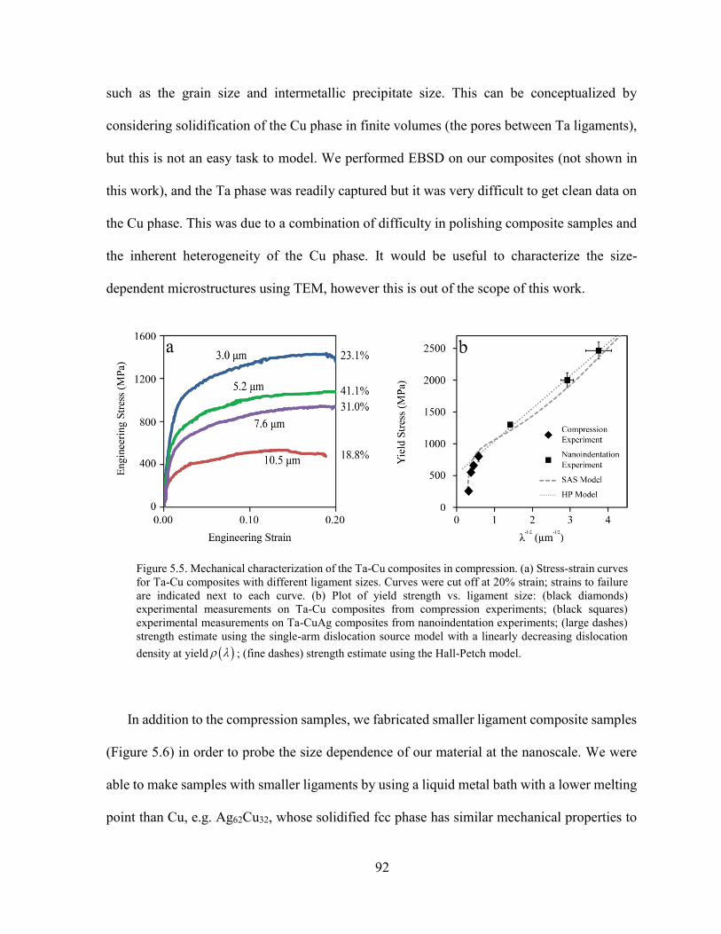
92

such as the grain size and intermetallic precipitate size. This can be conceptualized by

considering solidification of the Cu phase in finite volumes (the pores between Ta ligaments),

but this is not an easy task to model. We performed EBSD on our composites (not shown in

this work), and the Ta phase was readily captured but it was very difficult to get clean data on

the Cu phase. This was due to a combination of difficulty in polishing composite samples and

the inherent heterogeneity of the Cu phase. It would be useful to characterize the size-

dependent microstructures using TEM, however this is out of the scope of this work.

In addition to the compression samples, we fabricated smaller ligament composite samples

(Figure 5.6) in order to probe the size dependence of our material at the nanoscale. We were

able to make samples with smaller ligaments by using a liquid metal bath with a lower melting

point than Cu, e.g. Ag62Cu32, whose solidified fcc phase has similar mechanical properties to

Figure 5.5. Mechanical characterization of the Ta-Cu composites in compression. (a) Stress-strain curves

for Ta-Cu composites with different ligament sizes. Curves were cut off at 20% strain; strains to failure

are indicated next to each curve. (b) Plot of yield strength vs. ligament size: (black diamonds)

experimental measurements on Ta-Cu composites from compression experiments; (black squares)

experimental measurements on Ta-CuAg composites from nanoindentation experiments; (large dashes)

strength estimate using the single-arm dislocation source model with a linearly decreasing dislocation

density at yield ; (fine dashes) strength estimate using the Hall-Petch model.

93

Cu, Table 5.3. We assessed these materials using nanoindentation and estimated the yield

strength using 2.65y H . The materials were exceptionally hard and the data is included

in Figure 5.5b along with the yield strength data from compression testing.

In order to understand our material’s size dependent strengthening we compared the yield

strength data to two popular strengthening models used for nanostructured materials: the

single arm source dislocation model and the Hall-Petch model. The parameters used in the

following discussion can be found in Table 5.3. The single arm source model is used to

describe the strengthening behavior in single-crystal micropillars, and the critically resolved

shear stress CRSS is given by

0 0.5 lnCSRR

bb b

(5.1)

Figure 5.6. Ta composites were fabricated with smaller ligament sizes using a CuAg (~780 oC melting

point) liquid metal bath. (A) ~500 nm Ta-CuAg nanocomposite. (B) ~70 nm Ta-CuAg nanocomposite.

The 50 nm final polishing step can cause damage to surface ligaments when the ligaments are of a

comparable size.

94

where 0 is the lattice friction stress, is the shear modulus, b is the magnitude of the

Burgers vector, is the dislocation density at yielding, is a geometric constant with a value

0.12 , and is the average length of the weakest single arm dislocation source (131). The

Hall-Petch model is used to describe the strengthening behavior in nanocrystalline and

multilayer materials, and reasonably captures the data for layers and grain sizes larger than 100

nm. The yield strength y is given by

1 2

0y kh (5.2)

where, 0 is the lattice friction stress, k is the strengthening coefficient, and h is the

characteristic lengthscale of the microstructure (typically grain size but ligament diameter in

our case) (132).

The Hall-Petch model does not fit our large ligament data, as the yield strength has a

clear non-linear relationship with 1 2 , but we see good agreement with our smaller ligament

samples (3 µm, 500 nm, 117 nm, 70 nm), yielding 0.51k MPa m , and 0 530MPa . The

value of 0 is higher than our largest ligament sample, but is comparable to a rule of mixtures

estimate 559Ta Cu

y MPa using the yield strength of Ti20Ta80 and Cu25Ti75 (Table 5.3). The

strengthening coefficient for the composite is slightly higher than either component,

0.31Tak MPa m , and 0.14Cuk MPa m , but is still in reasonably good agreement (133).

The single arm source model captures the significant size-dependent strengthening we

see at all composite lengthscales under the hypothesis that the dislocation density at yield is

itself a function of the ligament size. This is a similar analysis to Conrad who proposed the

Hall-Petch effect is the result of a higher dislocation density at smaller grain sizes (134–136);

this is simply the result of considering smaller slip lengths in finite volumes. In this model, for

95

a given strain the dislocation density the dislocation density follows a 1 2d relationship.

Adding a similar relationship we produce a modified single arm source model that accounts

for constrained volumes because we qualitatively expect significant pile up in our composites.

Fitting the model to the yield strength for the 10.5 µm ligament sample we estimate a

dislocation density at yield of 13 27.0 10 m , and fitting the model to match the yield

strength for the 70 nm ligament sample yields an increased dislocation density of

15 21.4 10 m . Plotting the dislocation density at yield versus ligament size shows a linear

increase in the dislocation density with decreasing . This estimated range of values for

dislocation densities in the composites are reasonable, and consistent with dislocation densities

reported for micropillars (75, 127).

96

In the composites here, the Ta phase is essentially a single crystal, but the Cu phase is

polycrystalline, and one mechanism (single arm source or Hall-Petch) may dominate

depending on the ligament size. Each phase in the composite is geometrically constrained so

we expect both phases to have the same strain, Ta Cu , but we do not expect both phases to

have the same stress because they do not have equal volume fractions. This is a complex system

and it is not obvious that Equations (5.1) or (5.2) can fully capture dislocation evolution and

interactions in these bicontinuous composites without refinement. Regardless of the

Table 5.3 Material parameters used in our analysis.

Material ( )y MPa ( )E GPa

( )GPa

(A)b

3( )g cm

0 ( )MPa

Cu90Ti10 566 48* 159 6*

61 2** 2.556Cu 7.25* 34.8Cu

Cu75Ti25 900 52* 142 11* 55 4**

2.556Cu

6.75* 34.8Cu

Ti20Ta80 376 41* 200 10* 77 4**

2.83Ta 9.55* 47Ta

Ta/Cu 442ROM

559ROM

180 10* 69 4**

2.68RoM

8.8* 40RoM

Ta/CuAg

(500 nm)

1300 33*** 170 6* 65 2** - - -

Ta/CuAg

(117 nm)

1200 117*** 158 12* 61 5** - - -

Ta/CuAg

(70 nm)

2466 133*** 175 10* 67 4** - - -

CuAg 220 16*** 157 6*

60 2**

- - -

* -Experimentally measured

** -Estimated from experimental using the relationship: 2.6E

*** -Converted from hardness using the relationship: / 2.65y hardness

GA-Gibson-Ashby estimate

Cu-Property of elemental Copper (115), Ta-Property of elemental Tantalum (140)

ROM-Rule of mixtures estimate

97

strengthening mechanism(s), excavation of the dealloyed refractory phase after deformation

shows evidence of dislocation activity through the presence of slip traces (Figure 5.7a,b) in the

Ta phase. The Ta ligaments (Figure 5.7c) have obvious Cu-rich inclusions (confirmed by EDS)

that result from Rayleigh instabilities during coarsening and are not seen in the parent alloy

(35).

Similar to coated micropillars or passivated thin films, dislocation activity in the NPM

composite was neither stochastic nor catastrophic (128, 137, 138). For these reasons, the

composites studied here are able to strain harden and support large plastic strains, and

ultimately fail via delamination within grains (Figure 5.7c). Moreover, the composite

architecture allows for incorporation of size-scale effects without the collapse that occurs in

cellular materials and foams (111). Previous studies on the mechanical properties of dealloyed

nanoporous metals show that individual ligaments are ductile, but the overall structure is not

able to undergo significant macroscopic plastic deformation in tension (58, 61). Plasticity has

been reported in compression, with densification, dislocation motion, and dislocation storage

occurring simultaneously (56). In contrast, the fully-dense network microstructure of our bulk

composites manifests size-dependent mechanical properties associated with the internal

lengthscales that evolved during dealloying without any additional strain associated with

densification.

98

5.4.1.2 Microtensile Results

Due to a difficulty in sample preparation, we only tested a small number of Ta/Cu samples,

3 of which were ductile. The three ductile samples were from a preliminary batch and the four

brittle samples were from a second batch of dealloyed samples. We will discuss in the

following section the origins of ductile and brittle behavior in these materials, but for now we

will refer the reader to Figure 5.8 and Figure 5.9 to show how drastically different the two

batches were. Table 5.4 includes the yield strength data determined from the samples tested in

tension along with Ta and Cu references.

The average ligament size of the samples was ~ 6 µm and the average yield strength of the

ductile samples was ~ 645 MPa , which agrees well with the observed trend in our

compression measurements (our modified SAS model predicts 6 600y m MPa ). Figure

5.10 compares a stress-strain curve of the Ta/Cu composite to curves for pure Ta and pure Cu.

The composite is stronger than either component (although these are not representative

components), but is not as ductile. During all load tests the grips often lagged and we did not

have good correlation with the DIC software during the initial loading. As a result the modulus

Figure 5.7. Deformed Ta-Cu composites. (a) SEM micrograph of the deformed composite. (b) SEM

micrograph of the dealloyed Ta phase, excavated after deformation. (c) SEM micrograph of a deformed

Ta-Cu composite near to failure, showing delamination between the Ta and Cu phases.

99

values during the initial loading are not accurate and the modulus needed to be determined

during load/unload cycles. The load/unload cycles resulted in accurate modulus values for the

Ta and Cu samples, but we observed a hysteresis during two load/unload cycles for one of the

three Ta/Cu samples (Figure 5.11), and measured a very low modulus value ( ~ 75 GPa ). It is

possible there is time-dependent behavior associated with reversible twinning in the Cu phase

or destruction of the Ta/Cu interface, but we need to perform more tests to conclusively

determine what happened.

Interestingly, all of the composites experienced their maximum stress at yield. Once the

samples began to yield the behavior was almost perfectly plastic. In compression we observed

work hardening at all ligament sizes, but we do not have enough statistics to conclude the

behavior in tension. In section 4.4.7 we discussed how the connectivity of the structure is

strongly dependent on composition, time, and temperature; it is possible the samples we tested

in tension did not have a high enough connectivity to take advantage of the interlocked

structure. This work was performed before our in-depth kinetic study and it will be worthwhile

to revisit these experiments with our new knowledge base. Large batches of samples for

microtensile testing can dipped into baths of Cu and the microstructure can be more finely

tuned. Nevertheless, it is quite promising that some of the tensile samples were ductile because

this is the first reporting of a ductile nanoporous material.

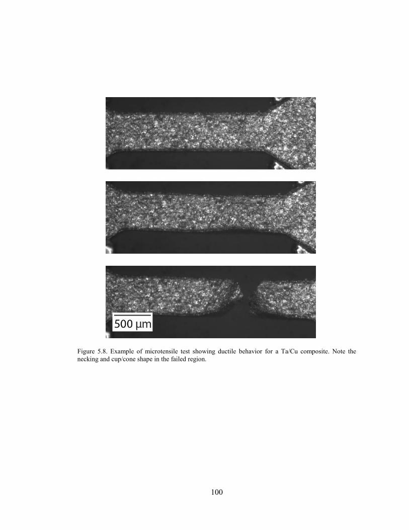
100

Figure 5.8. Example of microtensile test showing ductile behavior for a Ta/Cu composite. Note the

necking and cup/cone shape in the failed region.

101

Figure 5.9. Example of microtensile test showing a ductile behavior for a Ta/Cu composite. Note the

sharp crack at ~45o angle and lack of plastic deformation in the sample.

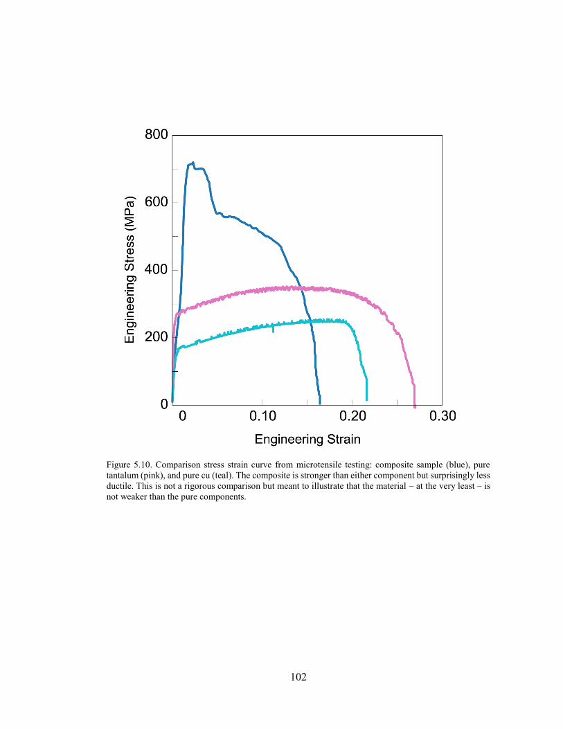
102

Figure 5.10. Comparison stress strain curve from microtensile testing: composite sample (blue), pure

tantalum (pink), and pure cu (teal). The composite is stronger than either component but surprisingly less

ductile. This is not a rigorous comparison but meant to illustrate that the material – at the very least – is

not weaker than the pure components.

103

Figure 5.11. Stress strain curve for one of the Ta/Cu composite samples where two unload/load cycles

were performed. There was significant lag and a slight hysteresis in the behavior.

104

Table 5.4. Mechanical data from microtensile tests.

Sample Yield Strength

(MPa)

Maximum Stress

(MPa)

Modulus

(GPa)

Strain at Failure

Ta/Cu 1 720 * - 0.108

Ta/Cu 2 535 * - 0.164

Ta/Cu 3 683 * 74 0.069

Ta/Cu 4 255 * - 0.0015

Ta/Cu 5 225 * - 0.0028

Ta/Cu 6 170 * - 0.0029

Ta/Cu 7 142 * - 0.0012

Ta 1 230 363 180 0.269

Ta 2 215 352 175 0.35

Ta 3 210 366 - 0.22

Cu 1 120 237 85 0.30

Cu 2 110 220 80 0.224

Cu 3 112 254 - 0.216

*indicates same as yield strength

105

5.4.1.3 Grain Boundary Character

High tortuosity in the interface between the matrix and dealloyed phases helps delay direct

delamination between phases and early failure as seen in multilayers (139) and allows for large

strains compared to the constituent phases alone. However, there are still subtle effects of the

structure of grain boundaries on work hardening and failure at scales much larger than the

ligaments (Figure 5.12). For instance, within a batch of compression samples with 7 μm feature

sizes, all had the same yield strength, but some samples underwent significant deformation –

over 65% strain – and significantly work hardened to compressive engienering stresses near

2.0 GPa without failing while others failed at ~950 MPa and 31% strain (Figure 5.12a). Similar

effects were observed in microtensile tests (Figure 5.12b): samples with identical feature sizes

and compositions had drastically different plasticity behaviors. Unlike in compression, where

all samples underwent some amount of plastic deformation, microtensile specimens were

either ductile or brittle.

The primary difference between the samples in Figure 5.12c,d and the samples in Figure

5.12e,f was their grain boundary structure. The high-strength, large-strain samples all showed

Ta-rich grain boundaries interconnecting adjacent grains Figure 5.12c,d) in contrast to

“detached” grain boundaries seen in the weaker samples (Figure 5.12e,f). The Ta grains in our

nanocomposites are quite large, ~500 µm in diameter, and only a few are needed to span the

microtensile and compression samples. We speculate that cracks can easily propagate along

the "detached" grain boundaries, and interconnected boundaries add fracture resistance. We

showed in Figure 5.7c that if the material does not fail prematurely at a grain boundary it

eventually fails via delamination between the matrix and dealloyed phases. This dependence

on grain boundaries is troubling from a materials fabrication perspective but we think that this

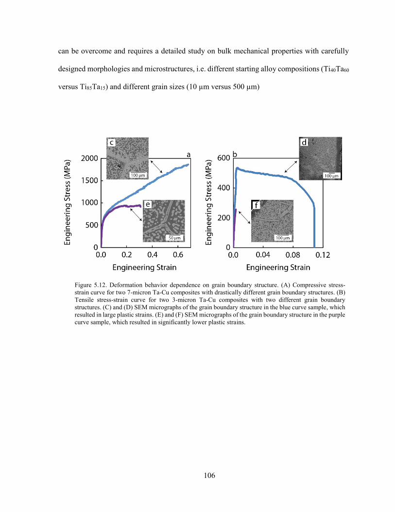
106

can be overcome and requires a detailed study on bulk mechanical properties with carefully

designed morphologies and microstructures, i.e. different starting alloy compositions (Ti40Ta60

versus Ti85Ta15) and different grain sizes (10 µm versus 500 µm)

Figure 5.12. Deformation behavior dependence on grain boundary structure. (A) Compressive stress-

strain curve for two 7-micron Ta-Cu composites with drastically different grain boundary structures. (B)

Tensile stress-strain curve for two 3-micron Ta-Cu composites with two different grain boundary

structures. (C) and (D) SEM micrographs of the grain boundary structure in the blue curve sample, which

resulted in large plastic strains. (E) and (F) SEM micrographs of the grain boundary structure in the purple

curve sample, which resulted in significantly lower plastic strains.

107

5.4.2 Tungsten-based compositions

5.4.2.1 Compression and Hardness Testing

We were also interested in studying the mechanical properties of W/Cu composites because

we can fabricate smaller ligament samples than Ta/Cu composites without needing to use lower

temperature baths. An additional benefit is that W/Cu is more of a classic composite material,

consisting of a hard brittle phase (W) and a ductile soft phase (Cu).

We fabricated compression samples of W/Cu composites with ~650 nm and ~1.1 μm

ligaments, but the dealloying was too sluggish to reliably create samples for compression

testing with smaller ligaments. Microhardness testing was used to measure the properties of

the smaller ligament sizes and we plotted the hardness versus ligament size in Figure 5.13. We

converted the compression yield strength values to a hardness value because the majority of

the data were hardness measurements, and used the relation from section 5.2.1, 2.65y H .

Performing a Hall-Petch fit we determined / 0.77W Cuk MPa m and 0 1GPa , compared

to 0.14Cuk MPa m and 3.1Wk MPa m . A rule of mixtures estimate for the composite

yields / 0.81W Cuk MPa m , in close agreement.

It is obvious that with decreasing ligament size the composite becomes stronger than either

of these estimates. We did not include a GA analysis for the bulk composite because we

showed in section 5.4.1.1 that deformation in the composite is very different from the porous

material. For comparison we included two rule of mixtures estimates for the hardness of the

bulk W/Cu composite. There are two estimates because the composition of the Cu phase varied

significantly depending on the ligament size, with smaller ligaments being associated with

higher Ti concentrations. Table 5.5 shows that although the CuTi compositions were quite

different the hardness values of the Cu75Ti25, Cu65Ti35, Cu50Ti50, compositions were nearly

108

identical. For ans estimate of the W phase we measured a hardness value of 4.6 .2 GPa for

pure tungsten. In any case these values appear to be a good lower bound for the W/Cu

composite materials.

Figure 5.13. Hardness versus ligament diameter for W/Cu. Values measured from Vickers microhardness

(orange squares), yield strength from macrocompression (orange circles) converted to hardness, Hall-

Petch fit (orange dashed), upper and lower bounds rule of mixtures estimates (purple dashed).

Table 5.5. Summary of the Cu phase composition for the W-Cu ligament sizes tested

Ligament Size

(nm)

Cu-Ti atomic composition Vickers Hardness of the Cu phase

(HV)

30 15 50 50 390 20

49 7.5 65 35 380 18

109 21 75 25 386 22

200 40 75 25 386 22

1500 50 90 10 279 14

109

Interestingly, and unlike the Ta-Cu composites, we do not observe a significant increase in

strength until the ligament size is below ~ 250 nm. A similar trend has been reported in

compression and tension experiments on tungsten micro- and nanopillars (140). This decreased

sensitivity to the sample diameter was attributed to a higher lattice resistance to dislocation

motion in W at room temperature and a stronger size dependence should be expected above

the critical temperature for W (~760 oC). This behavior at larger ligament sizes strongly

suggests that the refractory phase dominates the mechanical properties of these materials, but

further studies varying the ratio of the two phases are necessary before a conclusion can be

made.

Despite the fact that W has a higher yield strength than Ta, the W/Cu composites are

weaker than Ta/Cu composites of equivalent sizes, Figure 5.5b. This is easily explained by

noting that the Ti-W parent alloys only had 25 at.% W whereas the Ti-Ta parent alloys had 35

at.% Ta. If we assume the strength increase is only due to the refractory phase we estimate the

yield strength for a W35/Cu65 composite with ~70 nm ligaments would be ~2860 MPa, which

would place it slightly stronger than the Ta35/Cu65 composite with ~70 nm ligaments (~2500

MPa). It is interesting to consider which phase is actually controlling the mechanical

properties, but we also need to factor in the morphology (ligament connectedness), the

composition of the ligaments (not always pure refractory), and the composition of the Cu phase

(anywhere between 70 and ~0 at.% Ti). Controlled studies varying these parameters are

forthcoming.

110

5.4.2.2 TEM and HRTEM Observations

Owing to their nm-scale ligaments and bulk sample size, W/Cu specimens were examined

at Tohoku University by Eric Xu and Professor Chen using Transmission Electron Microscopy

(TEM). The primary goal was to better understand the structure of our composites, however

we were particularly interested in the Ti concentration across the W/Cu interface given the

results from Chapters 3 and 4.

Figure 5.14a-c shows a TEM micrograph of a W/Cu composite with ~50-100 nm ligaments

and Figure 5.14d-g are elemental maps of the enclosed region, and Figure 5.14h is a color

EELS map highlighting the Ti concentration. Similar to the EDS mapping we performed for

Ta/Cu composites in Chapter 3, the W and Cu phases are distinctly separate. This is expected

because the two elements are immiscible, but the TEM elemental mapping demonstrates the

interface is very sharp and appears to only be several nm wide. Additionally, due to the slow

diffusion kinetics in this system the Ti concentration is quite high. This is beneficial because

according to Table 5.5 the Cu phase becomes stronger with increasing Ti concentration.

It is also possible the Ti concentration can improve the quality of the interface between the

W and Cu phases. Simulation work by our collaborators (not shown), which mirrored the

morphology work in Chapter 3, reported a dramatic decrease in the Ti concentration at the

interface from the Cu phase (high) to the refractory phase (low). During dealloying, Ti atoms

are dissolved locally, leading to a very low concentration in the W phase and a high

concentration in the Cu phase. In order to compare theory to experiments we prepared a W/Cu

sample for atom probe tomography, Figure 5.15. As expected the Ti concentration is higher in

the Cu phase although the concentration difference is marginal. Nevertheless, we can also

confirm that the interface between the two phases is quite small, ~3 nm wide.

111

Finally, high-resolution TEM (HR-TEM) was also performed to study the quality of the

interface between the two phases, which has been shown to be incredibly important for the

mechanical properties of multilayer materials (139, 141–143). HR-TEM micrographs in Figure

5.16a-h show that the interface between the two immiscible phases is semi-coherent. This is

not observed in fcc/bcc multilayer materials, such as Cu/Nb, where there are periodic misfit

dislocations between the two phases to account for the different crystal structures. The

difference between the composites here and multilayer materials is how they are fabricated.

Multilayer materials are sputtered or evaporated (gas-to-solid growth) whereas the composite

materials in this work are solidified (liquid-to-solid growth) (132). This potentially allows for

a more benign crystallization, and thus a more coherent interface between the two phases. It

can be seen in the Fourier transforms in Figure 5.16c-h that the fcc Cu phase adopts an

orientation that matches closest with the W ligament’s crystal orientation. We did not perform

any TEM on deformed structures and are not able to comment whether this coherency aids in

plasticity across the layers or if dislocation activity is confined to each respective phase.

112

Figure 5.14. (a-c) HAADF STEM of W/Cu composite. (d-g) EDS mapping of region (c). (h) Color EELS

map showing concentration variation centered at a Ti-rich phase.

113

Figure 5.15. (a) FIB liftout of the ROI and shaped to needle (c) for atom probe tomography (APT). (b)

The reconstructed APT. (d) Line concentration profile across interface showing a sharp change between

the W and Cu phases.

114

Figure 5.16. Unfiltered HR-STEM images of the two phases, each phase were aligned along electron

beam directions. The K-S orientation relationship can be obtained

115

5.5 Summary and Conclusions

In this chapter we examined the mechanical properties of nanoporous metals and

bicontinuous composites. We showed that nanoporous metals have size-dependent

strengthening, but are weaker than expected because they are high-density metallic foams. This

challenge was overcome by creating fully-dense composite materials using liquid metal

dealloying. This work focused on Ta/Cu and W/Cu composites, but the results presented here

can extend to other liquid metal dealloying systems. We attempted to qualitatively explain this

by presenting a modified Taylor-strengthening law which included size-dependent terms for

truncated dislocation sources and dislocation densities. However, there is still significant work

left to be done before we can fully understand the underlying mechanisms in these materials.

Careful preparation of the Cu phase is necessary (grain size, volume fraction and size of CuTi

precipitates) in order to correctly report the size-dependent strengthening in these materials.

This chapter points the way to improvements in the mechanical properties of metals

through the design of bulk three-dimensional bicontinuous nancomposites, and these materials

will likely find many applications in structural applications that require high strength, ductility,

and high density of internal interfaces. The results presented in this chapter have been

published in (45).

116

Chapter 6 Conclusions and Future work

At the start of this thesis dealloying was limited to the fabrication of six relatively noble metals

(Ag, Au, Ni, Cu, Pt, and Pd), and the majority of studies focused on fabrication and the physical

properties of these nanoporous materials. Now, nearly every industrially relevant metal can

be made into a porous form factor using a dealloying process, Figure 6.1. This is largely due

to the innovation of liquid metal dealloying. We did not touch upon the possibility of using

Figure 6.1. Periodic table comparing the outlook of nanoporous metals made by dealloying at the time of

this thesis. (blue) Elements which have been successfully made porous via electrochemical dealloying.

(red) Elements which have been successfully made porous via liquid metal dealloying by Kato and

coworkers. (purple) Elements which can be made porous via liquid metal dealloying using the Ti-X

dealloying system in this work. (green) Other possible elements which can be made using other liquid

metal dealloying systems.

117

molten salts, however it is likely other elements not listed and new systems of elements

currently listed can be dealloyed using this technique.

The underlying motive of this work was to study the limits of dealloying and explore the

kinetics involved during pattern formation. Traditionally, work on dealloying is focused on

kinetics of the dissolving species, but the kinetics of the remaining species heavily influences

the properties and morphology of the final material; for example, the surface diffusivity of the

remaining species during dealloying dictates the length scale of the ligaments and pores.

Focusing on this concept we studied nanoparticle systems where the surface diffusion rate is

increased due to higher local curvatures, and dealloying of refractory systems where the

surface diffusion rate is much lower due to their high melting points. In addition, we studied

the mechanical properties of refractory-based composite materials.

It is important to remember that a dealloyed structure is metastable and will always undergo

coarsening to decrease its surface area. In fact, every dealloyed structure we experimentally

observe is a coarsened structure. For the case of np-Au it has been numerically calculated that

the initial roughening of the surface is ~ 1 nm, but observations of dealloyed films show ~ 10

nm ligaments, and bulk dealloyed samples (~ 1 mm3) show ~ 30 nm ligaments. As the

electrolyte penetrates deeper into the alloy, the previously dealloyed structure will coarsen

until the electrolyte is rinsed out. It follows that surface diffusion is the most important

parameter in dealloyed materials because it dictates the feature size as well as the ability, or

limit, of how large a sample can be made using a dealloyed technique.

During electrochemical dealloying, the critical potential represents the point where the

dissolution rate becomes comparable to the surface diffusion rate. The surface diffusivity has

been observed to change in different electrolyte solutions, and other tricks to control it have

118

been developed such as adding ternary components to the alloy to increase or decrease this

rate. We showed that the surface diffusion rate can change significantly in finite systems where

local curvatures, and thus local chemical potentials, dominate. Surface fluctuations become

short lived as the particle size decreases, and the critical potential needed to increase in order

to dealloy a system over this slower time period.

When attempting to fabricate a porous refractory material via dealloying we observed that

the surface diffusivity was too low to produce a coherent structure. Turning to the idea of the

homologous temperature, the reaction temperature necessary to produce np-Ta would ~ 400

oC. We were able to achieve this by developing our own variation of liquid metal dealloying.

Immersing Ti-rich refractory alloys into baths of Cu/Ag/Bi, we can span a dealloying

temperature range of 400 - 1600 oC, and fabricate ligaments across the range of 30 nm - 10

µm. It may be possible to fabricate Ta with 10 nm ligaments, but the homologous temperature

is only a rough guideline; due to coarsening it is not accurate to claim a specific ligament size

for a given homologous temperature, and the reported trend is only for structures that were

coarsened for extended periods of time.

From a superficial standpoint, liquid metal dealloying is identical to electrochemical

dealloying: a component is selectively dissolved while the other is allowed to remain and

diffuse along the metal/liquid interface. However, there are several key differences. First, the

characteristic morphology of electrochemically dealloyed materials is no longer present;

depending on the alloy composition, LMD can be used to produce droplets, lamellae, partially

connected structures, and fully connected structures. In full disclosure, we are not certain if we

can call any of these dealloyed structures bicontinuous. Possibly owing to the bcc lattice –

which has fewer nearest neighbor diffusion pathways – we observed significant amounts of

119

enclosed regions that are the results of inverse Rayleigh instabilities; future work will need to

address the topologies in these different structures. Second, the rate limiting step during LMD

is diffusion of the dissolving component away from the interface. In electrochemical

dealloying it has been extensively shown that the dissolution of a high coordinated site such as

a terrace atom is the rate-limiting behavior. Unlike liquid metal dealloying, once an atom is

dissolved it is rapidly transported away into the electrolyte solution. Third, the parting limit

appears to be much lower in LMD. Geometrically, the parting limit is considered to be the

space necessary for a surface atom to be complexed by ions in solution. Atoms in a liquid

metals are less “clunky” than metal-anion complexes and it is reasonable to expect the parting

to be lower. These differences lead to interesting implications for LMD. Because dissolution

is not rate-limiting the dealloying velocity is very fast, however it decays with time following

1 2~ t relationship. Electrochemical dealloying of bulk Ag-Au samples (~1 mm3) can take

several hours, or days, whereas LMD can accomplish this in several minutes. This is partially

due to significantly higher temperatures, but the different mechanism is the primary reason.

After we sufficiently understood how to dealloy refractory-based alloys we chose to

focus on the mechanical properties of these materials. The mechanical behavior of np-metals

has been extensively studied due to their unique form factor (a self-assembled bulk

nanostructure), but little work has been done to effectively explain the origin of the strength of

these materials. Compiling all of the current mechanical data we plotted the yield strength

(mostly converted from hardness values) versus ligament size. Unfortunately there was

significant scatter sample-to-sample, but this was understood by considering np-metals to be

foams which have reduced strengths and moduli from their bulk counterparts. After

normalizing the materials by their relative densities the data collapsed and an obvious size-

120

dependence appeared. The size-dependent strengthening was similar to single crystal

micropillars, however it is important to emphasize that the raw yield strength data have

generally low values. In order to fully utilize the strength effect from these small-scale

ligaments the void space needs to be filled with a secondary phase.

Serendipitously, a secondary phase infiltrates the porous material during liquid metal

dealloying. These composite materials were quite strong, showing increasing strength with

decreasing ligament size but we believe the more interesting feature of these materials are their

high interfacial area and interconnected structure. It has been shown that materials with high

interfacial areas are excellent candidates for radiation-damage tolerance. The high surface area

acts as a large sink for defects, and the inherent tortuosity of the composite should lead to a

relatively high toughness; the curvature requires a propagating crack to change its path

frequently, making failure difficult.

Looking towards the future of these materials, one of the largest challenges remaining in

the field of nanoporous metals made via dealloying is controlling coarsening that can occur

while the remainder of the material is being dealloyed. As shown in Chapter 4 this is extremely

important for liquid metal dealloying systems: the ligament size at the dealloying interface is

~ 80 nm, however the structure coarsens to ~ 1 µm in one second. Coarsening can also play a

role in the grain boundary structure, leading to weaker, detached structures at longer coarsening

times. There have been many recent papers on adding ternary components to suppress

coarsening from several research groups and we believe a solution to this issue is coming soon

(107, 144–146). Nevertheless, this work points towards the fabrication of new materials and a

new class of composite materials, all of which show promising results.

121

Appendix A

A.1 Table of Mechanical Data

Table A.1. Yield strength values adapted from literature values of nanoporous gold.

Relative

Density

Ligament

Diameter (nm)

Yield

strength

(MPa)*

Test Ref

0.2 20 24 Hardness (46)

0.25 10 62 Hardness -

0.25 30 19 Hardness -

0.25 50 14 Hardness -

0.3 40 32 Hardness -




0.3 160 15 Hardness -




0.33 40 83 Hardness -

0.35 100 69 Hardness -

0.35 19.3 37 Hardness (66)

0.42 19 64 Hardness -

0.42 19 87 Hardness -

0.2675 20 19 Hardness (56)

0.2675 27.5 14 Hardness -

0.2675 35 14 Hardness -

0.2675 40 12 Hardness -

0.2675 50 9 Hardness -

0.2675 55 10 Hardness -

0.2675 70 8 Hardness -

0.2675 250 3 Hardness -

0.4 5 373 Hardness (118)

0.4 29 279 Hardness -

0.4 126 196 Hardness -

0.25 10 65 Hardness (47)

0.25 25 20 Hardness -

0.25 50 12 Hardness -

0.42 100 55 Hardness -

0.36 15 30 Hardness (51)

0.36 13 38 Hardness -

0.36 14 50 Hardness -

122

0.359 32 42 Hardness (69)

0.35 59 40 Hardness (66)

0.35 56 41 Hardness -

0.35 75 34 Hardness -

0.35 58 47 Hardness -

0.35 55 47 Hardness -

0.35 95 30 Hardness -

0.35 60 50 Hardness -

0.35 60 26 Hardness -

0.35 198 19 Hardness -

0.275 15 27 Compression (56)

0.26 55 8 Compression -

0.33 15 100 Compression (57)

0.3 40 40 Compression (47)

0.3 23 16 Compression (58)

0.33 59.45 22 Tension (61)

0.33 32.8 27 Tension -

0.3 23 12 Tension (58)

0.352 32 65 Tension (69)

0.25 1.8 175 Simulation (62)

0.25 1.8 25 Simulation -

0.24 3.26 130 Simulation (71)

0.27 3.26 137 Simulation -

0.3 3.26 161 Simulation -

0.33 3.26 174 Simulation -

0.36 3.26 235 Simulation -

0.297 3.16 18.2 Simulation (63)

*yield strength for hardness data was estimated using the relationship 2.65y H

“-“ indicates data is from the same the reference above it

123

Appendix B

B.1 Concentration Profile

Consider an isothermal system containing an infinite liquid bath of Cu (concentration Tic

) and a semi-infinite block of Ti-Ta (concentration Ti

Sc ) where s t is the interface between

the two phases and 0 0s . When 0t , the Cu phase dissolves Ti from the TiTa alloy,

moving the interface in the positive x direction. We assume diffusion in the solid is frozen so

Ti

Sc is constant for all t . We also assume this process is near equilibrium and is constant for a

given Ti-Ta composition for all t .

There are two possible boundary conditions for the liquid phase: first, the bath is much

larger than the sample so the concentration of the liquid does not change over time and is

always its initial value , Tic t c ( 0Tic corresponds to a bath of pure Cu, but the Cu-

Ti phase diagram indicates the bath could reasonably be any CuxTi1-x concentration where

30x at.%); second, 0, Tic x t c , which accounts for electromagnetic mixing from the

RF induction coils pulling Ti away from the edge of the sample.

Summarizing our system we have:

Solid, s t x

, Ti

Sc x t c

Liquid, x s t

, Tic t c , or 0, Tic x t c

Boundary, x s t

0 0s

124

, Ti

Lc s t t c . (B.1)

In order to solve for ,c x t we rescale the problem using the substitution 2 L

x

D t and

define a function , ,F x t c x t . Eq. (4.1) becomes:

2

20

L

x dF d F

d dD t (B.2)

with the solution

12

2

CF erf C

12,

2 22 LL

x C xc x t F erf C

D tD t

. (B.3)

Using our boundary conditions from Eq. (B.1) and the solution from Eq. (B.3) we have

two possible solutions depending on the liquid phase boundary condition:

,2

1 12 2

Ti Ti Ti Ti

L L

L

L L

c c x c cc x t erf

D ts t s terf erf

D t D t

(B.4)

,2

2

Ti TiTiL

L

L

c c xc x t erf c

D ts terf

D t

(B.5)

Figure 4.4 compares the raw data along with fits for Eqs. (B.4) and (B.5) using a literature

value for the diffusivity of Ti in molten Cu, 5 2 1(1240 ) 7.0 10Ti CuD C cm s

. It is readily

apparent that the best fit is Eq. (B.5), which assumes that the edge of the sample will always

have the same Ti concentration as the liquid, i.e. 0, Tic x t c . This is a reasonable

125

assumption because induction melting induces eddy currents, which add convection to system.

We can further simplify Eq. (B.5) by defining a variable

2 L

s t

D t , yielding:

,2

Ti TiTiL

L

c c xc x t erf c

erf D t

. (B.6)

Eq. (B.6) is the final form for the concentration in the liquid phase. can be solved

numerically by fitting Eq. (B.6) to experimental data or analytically using the derivation in

Appendix A.2.

B.2 Dealloying Depth

We can use Eq. (4.2) to derive a relationship for the dealloying depth. First we define the

time derivative of the interface:

LDds

dt t

(B.7)

and the spatial derivative of Eq. (B.6) is given by

2 24

,Ti Ti x Dt Ti Ti

L L

L L

c c c e c c es t t

x erf erfD t D t

. (B.8)

Eq. (4.2) becomes

2

( ),

Ti TiTi Ti Ti TiL L LS L S L L

L

Dds c D c c ec c c c D s t t

dt x erft D t

(B.9)

and the analytical solution for is

2Ti Ti

L

Ti Ti

S L

c cerf e

c c

. (B.10)

126

We determined λ for each composition using Eq. (B.10) and the values for Ti

Lc and Ti

Sc ,

which were measured using EDS, and these values can be found in Table 4.1. Now that we

have solved for we can explicitly write the expression for the interface

24 Ls t D t . (B.11)

127

Appendix C

C.1 Complete Compression Data and DIC Analysis

Digital image correlation was used to determine the engineering strain in the compression

and tensile testing (130). The samples did not need any surface patterning because the recast

layer from the EDM provided a textured surface that was easy to track with the DIC software,

Figure C.1.

The recast layer was measured to only be ~ 10 µm, which contributes a negligible error to the

stress measurement for the bulk compression samples. At the beginning stages of this work we

tested the reliability of the DIC software and what was the appropriate resolution to accurately

track the strain. For the sample shown in Figure C.1 we chose different pixel resolutions for

tracking and compared the measurements to those directly measured from the images, Figure

Figure C.1. Ta/Cu sample for compression testing. (a) Initial sample, (b) sample after 200 seconds of

deformation, ~ 4 % strain.

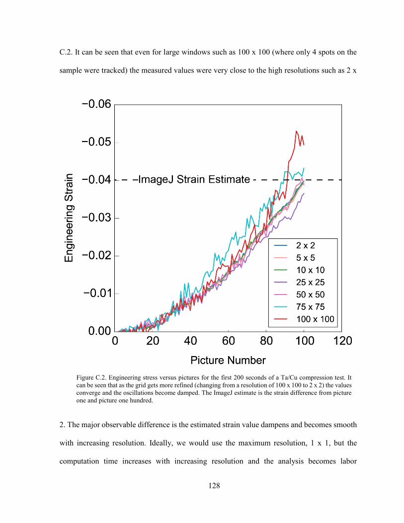
128

C.2. It can be seen that even for large windows such as 100 x 100 (where only 4 spots on the

sample were tracked) the measured values were very close to the high resolutions such as 2 x

2. The major observable difference is the estimated strain value dampens and becomes smooth

with increasing resolution. Ideally, we would use the maximum resolution, 1 x 1, but the

computation time increases with increasing resolution and the analysis becomes labor

Figure C.2. Engineering stress versus pictures for the first 200 seconds of a Ta/Cu compression test. It

can be seen that as the grid gets more refined (changing from a resolution of 100 x 100 to 2 x 2) the values

converge and the oscillations become damped. The ImageJ estimate is the strain difference from picture

one and picture one hundred.

129

intensive. For the majority of tests we used a 10 x 10 resolution, and occasionally cross-

checked the measurements with ImageJ and higher resolution runs. The remainder of this

section includes the compiled stress-strain data from the compression measurements.

Figure C.3. Engineering stress-strain curves for Ta/Cu composites with 3 µm features.

130

Figure C.4. Engineering stress-strain curves for Ta/Cu composites with 5.2 µm features.

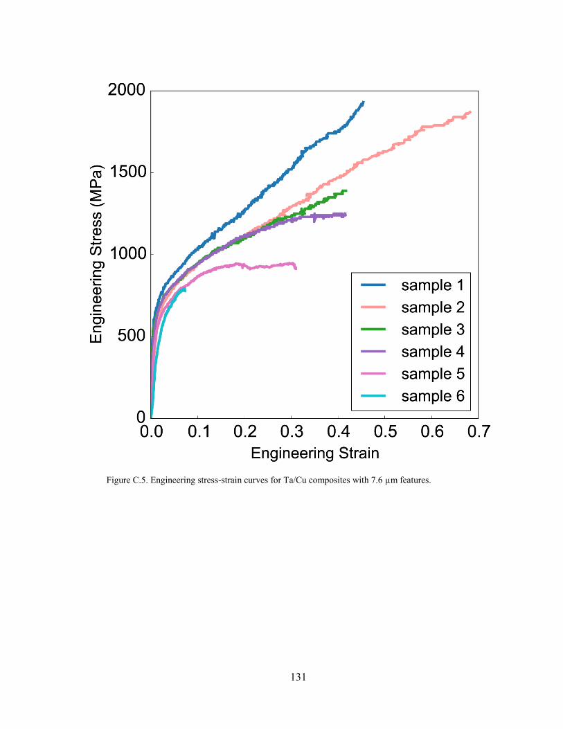
131


132


133

References

1. J. Snyder, K. Livi, J. Erlebacher, Oxygen Reduction Reaction Performance of

[MTBD][beti]-Encapsulated Nanoporous NiPt Alloy Nanoparticles. Adv. Funct. Mater.

23, 5494–5501 (2013).

2. K. Hu, D. Lan, X. Li, S. Zhang, Electrochemical DNA Biosensor Based on Nanoporous

Gold Electrode and Multifunctional Encoded DNA−Au Bio Bar Codes. Anal. Chem. 80,

9124–9130 (2008).

3. H. Jin, J. Weissmuller, A Material with Electrically Tunable Strength and Flow Stress.

Science (80-. ). 332, 1179–1182 (2011).

4. J. W. Kim et al., Optimizing niobium dealloying with metallic melt to fabricate porous

structure for electrolytic capacitors. Acta Mater. 84, 497–505 (2015).

5. X. Lang, A. Hirata, T. Fujita, M. Chen, Nanoporous metal/oxide hybrid electrodes for

electrochemical supercapacitors. Nat. Nanotechnol. 6, 232–236 (2011).

6. Y. Ito et al., High-quality three-dimensional nanoporous graphene. Angew. Chemie -

Int. Ed. 53, 4822–4826 (2014).

7. T. Wada et al., Bulk-nanoporous-silicon negative electrode with extremely high

cyclability for lithium-ion batteries prepared using a top-down process. Nano Lett. 14,

4505–4510 (2014).

8. J. Erlebacher, M. J. Aziz, a Karma, N. Dimitrov, K. Sieradzki, Evolution of

nanoporosity in dealloying. Nature. 410, 450–453 (2001).

9. J. Erlebacher, R. Seshadri, Hard Materials with Tunable Porosity. MRS Bull. 34, 561–

568 (2009).

10. K. Sieradzki, Curvature Effects in Alloy Dissolution. J. Electrochem. Soc. 140, 2868

(1993).

11. J. Erlebacher, K. Sieradzki, Pattern formation during dealloying. Scr. Mater. 49, 991–

996 (2003).

12. J. Snyder, T. Fujita, M. W. Chen, J. Erlebacher, Oxygen reduction in nanoporous metal-

ionic liquid composite electrocatalysts. Nat. Mater. 9 (2010), pp. 904–907.

13. F. Kertis et al., Structure/processing relationships in the fabrication of nanoporous gold.

JOM. 62 (2010), pp. 50–56.

14. H. Lechtman, Pre-Columbian Surface Metallurgy. Sci. Am. 250, 56–63154 (1984).

134

15. H. W. Pickering, Volume Diffusion During Anodic Dissolution of a Binary Alloy. J.

Electrochem. Soc. 115, 143 (1968).

16. A. J. Forty, Corrosion micromorphology of noble metal alloys and depletion gilding.

Nature. 282 (1979), pp. 597–598.

17. E. Seebauer, Estimating surface diffusion coefficients. Prog. Surf. Sci. 49, 265–330

(1995).

18. J. Rugolo, J. Erlebacher, K. Sieradzki, Length scales in alloy dissolution and

measurement of absolute interfacial free energy. Nat. Mater. 5, 946–949 (2006).

19. J. Erlebacher, An Atomistic Description of Dealloying. J. Electrochem. Soc. 151, C614

(2004).

20. J. Snyder, J. Erlebacher, Erratum: Kinetics of Crystal Etching Limited by Terrace

Dissolution [J. Electrochem. Soc., 157, C125 (2010)]. J. Electrochem. Soc. 157, S21

(2010).

21. H. W. Pickering, P. J. Byrne, On Preferential Anodic Dissolution of Alloys in the Low-

Current Region and the Nature of the Critical Potential. J. Electrochem. Soc. 118, 209

(1971).

22. D. M. Artymowicz, J. Erlebacher, R. C. Newman, Relationship between the parting

limit for de-alloying and a particular geometric high-density site percolation threshold.

Philos. Mag. 89, 1663–1693 (2009).

23. K. Sieradzki, R. R. Corderman, K. Shukla, R. C. Newman, Computer simulations of

corrosion: Selective dissolution of binary alloys. Philos. Mag. A. 59, 713–746 (1989).

24. R. C. Newman, R. R. Corderman, K. Sieradzki, Evidence for dealloying of austenitic

stainless steels in simulated stress corrosion crack environments. Br. Corros. J. 24, 143–

148 (1989).

25. K. Sieradzki et al., The Dealloying Critical Potential. J. Electrochem. Soc. 149, B370

(2002).

26. A. Dursun, D. V. Pugh, S. G. Corcoran, A Steady-State Method for Determining the

Dealloying Critical Potential. Electrochem. Solid-State Lett. 6, B32 (2003).

27. R. Mendoza, K. Thornton, I. Savin, P. W. Voorhees, The evolution of interfacial

topology during coarsening. Acta Mater. 54, 743–750 (2006).

28. Y. C. K. Chen-Wiegart et al., In situ imaging of dealloying during nanoporous gold

formation by transmission X-ray microscopy. Acta Mater. 61, 1118–1125 (2013).

135

29. Y. C. K. Chen-Wiegart et al., Structural evolution of nanoporous gold during thermal

coarsening. Acta Mater. 60, 4972–4981 (2012).

30. Y. C. K. Chen et al., Morphological and topological analysis of coarsened nanoporous

gold by x-ray nanotomography. Appl. Phys. Lett. 96, 213–215 (2010).

31. Y. C. K. Chen-Wiegart, S. Wang, I. McNulty, D. C. Dunand, Effect of Ag-Au

composition and acid concentration on dealloying front velocity and cracking during

nanoporous gold formation. Acta Mater. 61, 5561–5570 (2013).

32. Y. K. Chen-Wiegart et al., 3D morphological evolution of porous titanium by x-ray

micro- and nano-tomography. J. Mater. Res. 28, 2444–2452 (2013).

33. J. Erlebacher, I. McCue, Geometric characterization of nanoporous metals. Acta Mater.

60, 6164–6174 (2012).

34. T. Fujita, L. H. Qian, K. Inoke, J. Erlebacher, M. W. Chen, Three-dimensional

morphology of nanoporous gold. Appl. Phys. Lett. 92, 90–93 (2008).

35. J. Erlebacher, Mechanism of coarsening and bubble formation in high-genus

nanoporous metals. Phys. Rev. Lett. 106, 1–4 (2011).

36. K. Kolluri, M. J. Demkowicz, Coarsening by network restructuring in model

nanoporous gold. Acta Mater. 59, 7645–7653 (2011).

37. L. H. Qian, M. W. Chen, Ultrafine nanoporous gold by low-temperature dealloying and

kinetics of nanopore formation. Appl. Phys. Lett. 91, 083105 (2007).

38. H. Rösner, S. Parida, D. Kramer, C. A. Volkert, J. Weissmüller, Reconstructing a

Nanoporous Metal in Three Dimensions: An Electron Tomography Study of Dealloyed

Gold Leaf. Adv. Eng. Mater. 9, 535–541 (2007).

39. J. . Harrison, C. Wagner, The attack of solid alloys by liquid metals and salt melts. Acta

Metall. 7, 722–735 (1959).

40. T. Wada, K. Yubuta, A. Inoue, H. Kato, Dealloying by metallic melt. Mater. Lett. 65,

1076–1078 (2011).

41. M. Tsuda, T. Wada, H. Kato, Kinetics of formation and coarsening of nanoporous ??-

titanium dealloyed with Mg melt. J. Appl. Phys. 114, 113503 (2013).

42. T. Wada, H. Kato, Three-dimensional open-cell macroporous iron, chromium and

ferritic stainless steel. Scr. Mater. 68, 723–726 (2013).

43. K. Wang, J. Weissmüller, Composites of Nanoporous Gold and Polymer. Adv. Mater.

25, 1280–1284 (2013).

136

44. K. Wang et al., Nanoporous-gold-based composites: toward tensile ductility. NPG Asia

Mater. 7, e187 (2015).

45. I. McCue et al., Adv. Eng. Mater., in press, doi:10.1002/adem.201500219.

46. A. M. Hodge et al., Scaling equation for yield strength of nanoporous open-cell foams.

Acta Mater. 55, 1343–1349 (2007).

47. J. Biener et al., Size effects on the mechanical behavior of nanoporous Au. Nano Lett.

6, 2379–2382 (2006).

48. J. Weissmüller, R. C. Newman, H. Jin, A. M. Hodge, J. W. Kysar, Nanoporous Metals

by Alloy Corrosion: Formation and Mechanical Properties. MRS Bull. 34, 577–586

(2009).

49. I. C. Cheng, A. M. Hodge, Strength scale behavior of nanoporous Ag, Pd and Cu foams.

Scr. Mater. 69, 295–298 (2013).

50. J. Biener, A. M. Hodge, A. V. Hamza, Microscopic failure behavior of nanoporous gold.

Appl. Phys. Lett. 87, 1–3 (2005).

51. J. Biener, A. M. Hodge, A. V. Hamza, L. M. Hsiung, J. H. Satcher, Nanoporous Au: A

high yield strength material. J. Appl. Phys. 97, 024301–4 (2005).

52. L. a. Zepeda-Ruiz, B. Sadigh, J. Biener, A. M. Hodge, A. V. Hamza, Mechanical

response of freestanding Au nanopillars under compression. Appl. Phys. Lett. 91,

101907 (2007).

53. J. R. Hayes, a. M. Hodge, J. Biener, a. V. Hamza, K. Sieradzki, Monolithic nanoporous

copper by dealloying Mn–Cu. J. Mater. Res. 21, 2611–2616 (2006).

54. A. Hodge, J. Hayes, J. Caro, J. Biener, A. Hamza, Characterization and Mechanical

Behavior of Nanoporous Gold. Adv. Eng. Mater. 8, 853–857 (2006).

55. H.-J. Jin, D. Kramer, Y. Ivanisenko, J. Weissmüller, Macroscopically Strong

Nanoporous Pt Prepared by Dealloying. Adv. Eng. Mater. 9, 849–854 (2007).

56. H.-J. Jin et al., Deforming nanoporous metal: Role of lattice coherency. Acta Mater. 57,

2665–2672 (2009).

57. C. a. Volkert, E. T. Lilleodden, D. Kramer, J. Weissmuller, Approaching the theoretical

strength in nanoporous Au. Appl. Phys. Lett. 89, 061920 (2006).

58. T. J. Balk, C. Eberl, Y. Sun, K. J. Hemker, D. Gianola, Tensile and Compressive

Microspecimen Testing of Bulk Nanoporous Gold. JOM. 61, 26–31 (2009).

137

59. N. Abdolrahim et al., The mechanical response of core-shell structures for nanoporous

metallic materials. Philos. Mag. 93, 736–748 (2012).

60. Y. Sun, J. Ye, A. M. Minor, T. J. Balk, In situ indentation of nanoporous gold thin films

in the transmission electron microscope. Microsc. Res. Tech. 72, 232–241 (2009).

61. N. J. Briot, T. Kennerknecht, C. Eberl, T. J. Balk, Mechanical properties of bulk single

crystalline nanoporous gold investigated by millimetre-scale tension and compression

testing. Philos. Mag. 94, 847–866 (2014).

62. D. Farkas, A. Caro, E. Bringa, D. Crowson, Mechanical response of nanoporous gold.

Acta Mater. 61, 3249–3256 (2013).

63. N. D. Bao-Nam et al., Anomalous compliance and early yielding of nanoporous gold.

Acta Mater. 93, 144–155 (2015).

64. N. Huber, R. N. Viswanath, N. Mameka, J. Markmann, J. Weissmüller, Scaling laws of

nanoporous metals under uniaxial compression. Acta Mater. 67, 252–265 (2014).

65. H. L. Fan, D. N. Fang, Modeling and limits of strength of nanoporous foams. Mater.

Des. 30, 1441–1444 (2009).

66. N. J. Briot, thesis, University of Kentucky (2015).

67. R. Dou, B. Derby, Deformation mechanisms in gold nanowires and nanoporous gold.

Philos. Mag. 91, 1070–1083 (2011).

68. T. Wada, A. D. Setyawan, K. Yubuta, H. Kato, Nano- to submicro-porous β-Ti alloy

prepared from dealloying in a metallic melt. Scr. Mater. 65, 532–535 (2011).

69. D. Lee et al., Microfabrication and mechanical properties of nanoporous gold at the

nanoscale. Scr. Mater. 56, 437–440 (2007).

70. L. J. Gibson, M. F. Ashby, Cellular Solids: Structure and Properties (Cambridge

Univeristy Press, Cambridge, 1997).

71. X.-Y. Sun, G.-K. Xu, X. Li, X.-Q. Feng, H. Gao, Mechanical properties and scaling

laws of nanoporous gold. J. Appl. Phys. 113, 023505 (2013).

72. R. Dou, B. Derby, A universal scaling law for the strength of metal micropillars and

nanowires. Scr. Mater. 61, 524–527 (2009).

73. J. a. El-Awady, Unravelling the physics of size-dependent dislocation-mediated

plasticity. Nat. Commun. 6, 5926 (2015).

138

74. Q. Yu, R. K. Mishra, J. W. Morris, A. M. Minor, The effect of size on dislocation cell

formation and strain hardening in aluminium. Philos. Mag. 94, 2062–2071 (2014).

75. D. M. Norfleet, D. M. Dimiduk, S. J. Polasik, M. D. Uchic, M. J. Mills, Dislocation

structures and their relationship to strength in deformed nickel microcrystals. Acta

Mater. 56, 2988–3001 (2008).

76. H. J. Jin, J. Weissmüller, Bulk nanoporous metal for actuation. Adv. Eng. Mater. 12,

714–723 (2010).

77. H. J. Jin et al., Nanoporous au-pt alloys as large strain electrochemical actuators. Nano

Lett. 10, 187–194 (2010).

78. A. Wittstock, J. Biener, M. Bäumer, Nanoporous gold: a new material for catalytic and

sensor applications. Phys. Chem. Chem. Phys. 12, 12919–12930 (2010).

79. X.-L. Ye, H.-J. Jin, Electrochemical control of creep in nanoporous gold. Appl. Phys.

Lett. 103, 201912 (2013).

80. S.-M. Zhang, H.-J. Jin, Multilayer-structured gold/nanoporous gold composite for high

performance linear actuation. Appl. Phys. Lett. 104, 101905 (2014).

81. A. Mathur, J. Erlebacher, Size dependence of effective Young’s modulus of nanoporous

gold. Appl. Phys. Lett. 90, 061910 (2007).

82. L. Rong, Sieradzki, Ductile-Brittle Transition in Random Porous Au. Phys. Rev. Lett.

68, 1168–1171 (1992).

83. Y. Ding, M. Chen, J. Erlebacher, Metallic mesoporous nanocomposites for

electrocatalysis. J. Am. Chem. Soc. 126, 6876–6877 (2004).

84. J. Snyder, J. Erlebacher, in ECS Transactions (2011;

http://ecst.ecsdl.org/cgi/doi/10.1149/1.3635634), vol. 41, pp. 1021–1030.

85. D. Wang, P. Zhao, Y. Li, General preparation for Pt-based alloy nanoporous

nanoparticles as potential nanocatalysts. Sci. Rep. 1, 1–5 (2011).

86. S. Chen et al., Origin of oxygen reduction reaction activity on “Pt 3Co” nanoparticles:

Atomically resolved chemical compositions and structures. J. Phys. Chem. C. 113,

1109–1125 (2009).

87. S. Parida et al., Volume Change during the Formation of Nanoporous Gold by

Dealloying. Phys. Rev. Lett. 97, 035504 (2006).

88. T. Fujita et al., Unusually small electrical resistance of three-dimensional nanoporous

gold in external magnetic fields. Phys. Rev. Lett. 101, 1–4 (2008).

139

89. L. Tang et al., Electrochemical stability of nanometer-scale Pt particles in acidic

environments. J. Am. Chem. Soc. 132, 596–600 (2010).

90. L. Tang, X. Li, R. C. Cammarata, C. Friesen, K. Sieradzki, Electrochemical Stability of

Elemental Metal Nanoparticles. J. Am. Chem. Soc. 132, 11722–11726 (2010).

91. N. Combe, P. Jensen, A. Pimpinelli, Changing Shapes in the Nanoworld. Phys. Rev.

Lett. 85, 110–113 (2000).

92. S. a. Policastro et al., Surface Diffusion and Dissolution Kinetics in the Electrolyte–

Metal Interface. J. Electrochem. Soc. 157, C328 (2010).

93. Y. Ding, Y. J. Kim, J. Erlebacher, Nanoporous gold leaf: “Ancient technology

”/advanced material. Adv. Mater. 16, 1897–1900 (2004).

94. J. Snyder, K. Livi, J. Erlebacher, Dealloying Silver/Gold Alloys in Neutral Silver Nitrate

Solution: Porosity Evolution, Surface Composition, and Surface Oxides. J.

Electrochem. Soc. 155, C464 (2008).

95. T. P. Moffat, F. F. Fan, A. J. Bard, Electrochemical and Scanning Tunneling

Microscopic Study of Dealloying of Cu[sub 3]Au. J. Electrochem. Soc. 138, 3224

(1991).

96. I. McCue et al., Apparent Inverse Gibbs-Thomson Effect in Dealloyed Nanoporous

Nanoparticles. Phys. Rev. Lett. 108, 225503 (2012).

97. S. P. Lynch, Metal-induced embrittlement of materials. Mater. Charact. 28, 279–289

(1992).

98. S. P. Lynch, Solid-metal-induced embrittlement of aluminium alloys and other

materials. Mater. Sci. Eng. A. 108, 203–212 (1989).

99. M. H. Kamdar, Embrittlement by liquid metals. Prog. Mater. Sci. 15, 289–374 (1973).

100. M. G. G. Nicholas, C. F. F. Old, Liquid metal embrittlement. J. Mater. Sci. 14, 1–18

(1979).

101. Q. Chen, K. Sieradzki, Spontaneous evolution of bicontinuous nanostructures in

dealloyed Li-based systems. Nat. Mater. 12, 1102–6 (2013).

102. P.-A. Geslin, I. McCue, B. Gaskey, J. Erlebacher, A. Karma, “Topology-generating

Interfacial Pattern Formation During Liquid Metal Dealloying” (2015).

103. J. W. Kim, T. Wada, S. G. Kim, H. Kato, Sub-micron porous niobium solid electrolytic

capacitor prepared by dealloying in a metallic melt. Mater. Lett. 116, 223–226 (2014).

140

104. B. Šarler, Stefan’s work on solid-liquid phase changes. Eng. Anal. Bound. Elem. 16, 83–

92 (1995).

105. J. C. Dibbern, thesis, Massachusetts Institute of Technology (2007).

106. D. B. Butrymowicz, J. R. Manning, M. E. Read, Diffusion in copper and copper alloys.

Part III. Diffusion in systems involving elements of the groups IA, IIA, IIIB, IVB, VB,

VIB, and VIIB. J. Phys. Chem. Ref. Data. 4 (1975), p. 177.

107. X.-L. Ye et al., Primary and Secondary Dealloying of Au(Pt)-Ag: Structural and

Compositional Evolutions, and Volume Shrinkage. J. Electrochem. Soc. 161, C517–

C526 (2014).

108. K. Sieradzki, The fracture strength of solids near the percolation threshold. J. Phys. C

Solid State Phys. 18, L855–L856 (1985).

109. K. Sieradzki, The Relationship Between Dealloying and Transgranular Stress-Corrosion

Cracking of Cu-Zn and Cu-Al Alloys. J. Electrochem. Soc. 134, 1635 (1987).

110. T. a. Schaedler et al., Ultralight Metallic Microlattices. Science (80-. ). 334, 962–965

(2011).

111. L. R. Meza, S. Das, J. R. Greer, Strong, lightweight, and recoverable three-dimensional

ceramic nanolattices. Science (80-. ). 345, 1322–1326 (2014).

112. D. Jang, L. R. Meza, F. Greer, J. R. Greer, Fabrication and deformation of three-

dimensional hollow ceramic nanostructures. Nat. Mater. 12, 893–898 (2013).

113. K. J. Hemker, W. D. Nix, Seeing is believing. Nat. Mater. 7, 97 (2008).

114. J. R. Greer, J. T. M. De Hosson, Plasticity in small-sized metallic systems: Intrinsic

versus extrinsic size effect. Prog. Mater. Sci. 56, 654–724 (2011).

115. S.-W. Lee, W. D. Nix, Size dependence of the yield strength of fcc and bcc metallic

micropillars with diameters of a few micrometers. Philos. Mag. 92, 1238–1260 (2012).

116. J. R. Greer, W. C. Oliver, W. D. Nix, Size dependence of mechanical properties of gold

at the micron scale in the absence of strain gradients. Acta Mater. 53, 1821–1830 (2005).

117. Callister, Materials Science Engineering: An Introduction (Wiley).

118. M. Hakamada, M. Mabuchi, Mechanical strength of nanoporous gold fabricated by

dealloying. Scr. Mater. 56, 1003–1006 (2007).

119. C. a. Volkert, E. T. Lilleodden, Size effects in the deformation of sub-micron Au

columns. Philos. Mag. 86, 5567–5579 (2006).

141

120. Y. Sun, J. Ye, Z. Shan, A. M. Minor, T. J. Balk, The mechanical behavior of nanoporous

gold thin films. JOM. 59, 54–58 (2007).

121. H. Bei, S. Shim, G. M. Pharr, E. P. George, Effects of pre-strain on the compressive

stress–strain response of Mo-alloy single-crystal micropillars. Acta Mater. 56, 4762–

4770 (2008).

122. H. BEI et al., Compressive strengths of molybdenum alloy micro-pillars prepared using

a new technique. Scr. Mater. 57, 397–400 (2007).

123. R. Liu, A. Antoniou, A relationship between the geometrical structure of a nanoporous

metal foam and its modulus. Acta Mater. 61, 2390–2402 (2013).

124. M. M. Biener et al., Ultra-strong and low-density nanotubular bulk materials with

tunable feature sizes. Adv. Mater. 26, 4808–4813 (2014).

125. N. a Senior, R. C. Newman, Synthesis of tough nanoporous metals by controlled

electrolytic dealloying. Nanotechnology. 17, 2311–2316 (2006).

126. S. L. Choi, thesis, University of Toronto (2009).

127. R. Gu, a. H. W. Ngan, Effects of pre-straining and coating on plastic deformation of

aluminum micropillars. Acta Mater. 60, 6102–6111 (2012).

128. K. S. Ng, a. H. W. Ngan, Effects of trapping dislocations within small crystals on their

deformation behavior. Acta Mater. 57, 4902–4910 (2009).

129. D. Gianola, K. J. Hemker, M. Legros, W. N. Sharpe, Experimental Techniques for

Uncovering Deformation Mechanisms in Nanocrystalline Al Thin Films. TMS Lett. 1,

7 (2004).

130. C. Eberl, R. Thompson, D. S. Gianola, W. N. Sharpe, K. J. Hemker, Digital Image

Correlation (2006), (available at http://www.mathworks.com).

131. S. I. Rao et al., Estimating the strength of single-ended dislocation sources in micron-

sized single crystals. Philos. Mag. 87, 4777–4794 (2007).

132. a. Misra, J. P. Hirth, R. G. Hoagland, Length-scale-dependent deformation mechanisms

in incoherent metallic multilayered composites. Acta Mater. 53, 4817–4824 (2005).

133. K. T. Ramesh, Nanomaterials (Springer US, Boston, MA, 2009;

http://link.springer.com/10.1007/978-0-387-09783-1).

134. H. Conrad, K. Jung, Effect of grain size from mm to nm on the flow stress and plastic

deformation kinetics of Au at low homologous temperatures. Mater. Sci. Eng. A. 406,

78–85 (2005).

142

135. H. Conrad, Grain-size dependence of the flow stress of Cu from millimeters to

nanometers. Metall. Mater. Trans. A. 35, 2681–2695 (2004).

136. H. Conrad, S. Feuerstein, L. Rice, Effects of grain size on the dislocation density and

flow stress of niobium. Mater. Sci. Eng. 2, 157–168 (1967).

137. I. Ryu, W. Cai, W. D. Nix, H. Gao, Stochastic behaviors in plastic deformation of face-

centered cubic micropillars governed by surface nucleation and truncated source

operation. Acta Mater. 95, 176–183 (2015).

138. W. D. Nix, Mechanical properties of thin films. Metall. Trans. A. 20, 2217–2245 (1989).

139. N. A. Mara, D. Bhattacharyya, R. G. Hoagland, A. Misra, Tensile behavior of 40nm

Cu/Nb nanoscale multilayers. Scr. Mater. 58, 874–877 (2008).

140. J.-Y. Kim, D. Jang, J. R. Greer, Tensile and compressive behavior of tungsten,

molybdenum, tantalum and niobium at the nanoscale. Acta Mater. 58, 2355–2363

(2010).

141. E. G. Fu et al., Mechanical properties of sputtered Cu/V and Al/Nb multilayer films.

Mater. Sci. Eng. A. 493, 283–287 (2008).

142. N. Li et al., He ion irradiation damage in Fe/W nanolayer films. J. Nucl. Mater. 389,

233–238 (2009).

143. N. Li, N. A. Mara, Y. Q. Wang, M. Nastasi, A. Misra, Compressive flow behavior of

Cu thin films and Cu/Nb multilayers containing nanometer-scale helium bubbles. Scr.

Mater. 64, 974–977 (2011).

144. J. Snyder, P. Asanithi, A. B. Dalton, J. Erlebacher, Stabilized Nanoporous Metals by

Dealloying Ternary Alloy Precursors. Adv. Mater. 20, 4883–4886 (2008).

145. Z. Qi et al., Porous Gold with a Nested-Network Architecture and Ultrafine Structure.

Adv. Funct. Mater. 25, 2530–2536 (2015).

146. a. a. Vega, R. C. Newman, Nanoporous Metals Fabricated through Electrochemical

Dealloying of Ag-Au-Pt with Systematic Variation of Au:Pt Ratio. J. Electrochem. Soc.

161, C1–C10 (2013).

143

Vita

Ian McCue was born in Philadelphia, Pennsylvania and grew up outside of the city in

Yardley Borough. He graduated from Johns Hopkins University with a degree in Materials

Science and Engineering (2010), where his senior research design project was the fabrication

of single crystal aluminum oxide substrates for organic transistor devices. He joined Professor

Jonah Erlebacher’s research group at Johns Hopkins University in 2010 to pursue a Ph.D. in

Materials Science and Engineering studying the limits and tuenability of dealloying.

Publications

Manuscripts in Preparation (available upon request)

10. I. McCue, J. Erlebacher, “The Underlying Strength of Individual Phases in Metal/Metal

Bicontinuous Composites,” expected submission October 2015.

9. I. McCue, B. Gaskey, PA. Geslin, A. Karma, J. Erlebacher, “Kinetics of Liquid Metal

Dealloying: An Experimental Study,” expected submission September 2015.

Refereed Journal Publications

8. I. McCue, E. Benn, B. Gaskey, J. Erlebacher, “Dealloying and Dealloyed Materials,”

Annual Reviews of Materials Research, In Production.

7. PA. Geslin, I. McCue, B. Gaskey, A. Karma, J. Erlebacher, “Topology-generating

interfacial pattern formation during liquid metal dealloying,” Accepted (2015).

6. I. McCue, S. Ryan, K. Hemker, X. Xu, N. Li, M. Chen, J. Erlebacher, “Size Effects in the

Mechanical Properties of Bulk Bicontinuous Ta/Cu Nanocomposites Made by Liquid

Metal Dealloying,” Advanced Engineering Materials, Accepted (2015). DOI:

10.1002/adem.201500219.

5. X. Li, Q. Chen, I. McCue, J. Snyder, P. Crozier, J. Erlebacher, K. Sieradzki, “Dealloying

of Noble-Metal Alloy Nanoparticles,” Nano Letters, 14 (5), 2569-2577 (2014).

4. J. Erlebacher, I. McCue, "Geometric Characterization of Nanoporous Metals," Acta

Materialia, 60 (17), 6164–6174 (2012).

144

3. I. McCue, J Snyder, X Li, Q Chen, K Sieradzki, J Erlebacher, "Apparent Inverse Gibbs

Thomson Effect in Dealloyed Nanoporous Nanoparticles," Physical Review Letters, 108

(22), 225503 (2012).

2. J. Snyder, I. McCue, K. Livi, J. Erlebacher, "Structure/Processing/Properties Relationships

in Nanoporous Nanoparticles As Applied to Catalysis of the Cathodic Oxygen Reduction

Reaction," Journal of the American Chemical Society, 134 (20), 8633–8645 (2012).

1. J. Sun, O. Wilson, M. Reese, B.J. Jung, T. Dawidcyk, M. Yeh, B.M. Dhar, B.N. Pal, P.

Trottman, I. McCue, L. Berger, G.R. Blum, E. Heinemann, D. McGee, J.D. Erlebacher,

H.E. Katz, "Hands-on Preparation and Testing of Solution-Processed Semiconductor

Devices in the Undergraduate Classroom," Journal of Materials Education, 31 (5), 271-

284 (2009).

Presentations “*” denotes an invited presentation. Presenting authors are underlined.

Oral Presentations

9. I. McCue, B. Gaskey, P.-A. Geslin, A. Karma, J. Erlebacher, “Kinetics of Morphological

Evolution during Liquid Metal Dealloying” Materials Research Society Fall Meeting,

Boston, Massachusetts, to be presented December 2nd 2015 [Accepted].

8. I. McCue, S. Ryan, K. Hemker, J. Erlebacher, “Bulk Bicontinuous Ta/Cu Nanocomposites

Made by Liquid Metal Dealloying : Structure and Mechanical Properties,” Materials

Research Society Fall Meeting, Boston, Massachusetts, to be presented December 1st,

2015 [Accepted].

7. I. McCue, S. Ryan, K. Hemker, X. Xu, N. Li, M. Chen, J. Erlebacher, "Hierarchical,

Bicontinuous Refractory-Based Nanocomposites,” Materials Research Society Fall

Meeting, Graduate Student Award Talk, Boston, Massachusetts, December 2nd 2014

[Talk].

6. I. McCue, S. Ryan, K. Hemker, X. Xu, N. Li, M. Chen, J. Erlebacher, "Hierarchical,

Bicontinuous Refractory-Based Nanocomposites,” Materials Research Society Fall

Meeting, Boston, Massachusetts, December 1st 2014 [Talk].

5. I. McCue, S. Ryan, K. Hemker, X. Xu, N. Li, M. Chen, J. Erlebacher, "Mechanical

Properties of Hierarchical Refractory-Based Nanocomposites," First International

Symposium on Nanoporous Materials by Alloy Corrosion, Lake Bostol, Germany,

September 30th 2014 [Talk].

4. *J. Erlebacher, E. Benn, I. McCue, "Control of the Interface Mobility during Dealloying:

New Systems and New Materials,” Materials Research Society Fall Meeting, Boston,

Massachusetts, December 5th 2013 [Talk].

http://www.tuhh.de/t3resources/sfb986/documents/NPM_2014_technical_program.pdf






145

3. *I. McCue, J. Erlebacher, "Dealloying and Fabrication of Porous Tantalum," Gordon

Research Conference in Thin Film and Crystal Growth, Biddeford, Maine, July 9th 2013

[Talk]. Abstract was selected to give oral presentation.

2. I. McCue, J. Snyder, X. Li, Q. Chen, K. Sieradzki, and J. Erlebacher, "Apparent Inverse

Gibbs-Thomson Effect in Dealloyed Nanoporous Nanoparticles," Materials Research

Society Fall Meeting, Boston, Massachusetts, November 29th 2012 [Talk].

1. X. Li, I. McCue, J. Snyder, J. Erlebacher, K. Sieradzki, “Dealloying of Nanoparticles,”

Fall ECS Meeting, Honolulu, HI, October 11 2012 [Talk].

Poster Presentations

2. I. McCue, PA. Geslin, S. Ryan, K. Hemker, A. Karma, J. Erlebacher, "Bicontinuous

Refractory-Based Nanocomposites," Gordon Research Conference in Physical

Metallurgy, Biddeford, Maine, July 19th-24th 2015.

1. I. McCue, J. Erlebacher, "Liquid Metal Dealloying of Binary Refractory Alloys," Materials

Research Society Fall Meeting, Boston, Massachusetts, December 2nd 2013.

Patent

1. J. Erlebacher, I. McCue, "Nanostructured Composite Materials Containing Refractory

Elements," U.S. Patent Application Serial No. 13/975,659 filed on August 26, 2013

Frontiers Of Dealloying Novel Processing For Advanced ...

Documents

Transcript of Frontiers Of Dealloying Novel Processing For Advanced ...