Front Matter Template - University of Texas at Austin
115
DISCLAIMER: This document does not meet the current format guidelines of the Graduate School at The University of Texas at Austin. It has been published for informational use only.
Transcript of Front Matter Template - University of Texas at Austin

DISCLAIMER:
This document does not meet the current format guidelines of
the Graduate School at The University of Texas at Austin.
It has been published for informational use only.

Copyright
by
William Ladd Gurecky
2015

The Thesis Committee for William Ladd Gurecky
Certifies that this is the approved version of the following thesis:
Development of an MCNP6 - ANSYS FLUENT
Multiphysics Coupling Capability
APPROVED BY
SUPERVISING COMMITTEE:
Supervisor:
Erich Schneider
Steven Biegalski
Development of an MCNP6 - ANSYS FLUENT
Multiphysics Coupling Capability
by
William Ladd Gurecky, MSE
Thesis
Presented to the Faculty of the Graduate School of
The University of Texas at Austin
in Partial Fulfillment
of the Requirements
for the Degree of
Master of Science in Mechanical Engineering
The University of Texas at Austin
December, 2015

v
Acknowledgements
I acknowledge Andrew Godfrey, Ben Collins and Aaron Grahm for their guidance
in the use of VERA-CS and insight into multiphysics coupling problems. I appreciated
the lively and friendly atmosphere provided by those with whom I worked with at Oak
Ridge National Laboratory (ORNL). Most importantly, this work would not have been
possible without the direction and support of my primary academic advisor, Erich
Schneider.
Funding for this work was provided by the Consortium for Advanced Simulation
of LWR’s (CASL), a DOE innovation hub based at ORNL (contract No. DOE-
4000122526).

vi
Abstract
Development of an MCNP6 - ANSYS FLUENT
Multiphysics Coupling Capability
William Ladd Gurecky, MSME.
The University of Texas at Austin, 2015
Supervisor: Erich Schneider
This thesis presents a novel core multiphysics coupling method and its application
to geometries and thermal hydraulic operating conditions typical of U.S. PWRs. Monte
Carlo based radiation transport from the MCNP6 package and finite volume thermal
hydraulic (TH) packages provided by ANSYS-FLUENT are combined to produce results
with intra-pin resolved spatial resolution equivalent to state-of-the-art reactor physics and
multi-physics suites. The Virtual Environment for Reactor Applications (VERA) whose
development is spearheaded at Oak Ridge National Laboratory is one such example
package. Benchmark and validation tasks performed as an integral part of the
development of VERA demand intra-pin resolved pin power distributions as well as
finely spatially resolved fuel burnups. This level of detail is not provided by most other
lattice physics code packages. Intra-pin powers, for example, are reconstructed from
lower fidelity model results using empirically derived shape functions. In addition, data
sets from operating PWRs are sparse, resolved only at the inter-pin level, and prone to
experimental error. With the proposed MCNP-FLUENT model, it is possible to provide
within-pin/channel resolved power, temperature and moderator density field data.
MCNP-FLUENT iteratively solves for multiple physical fields: flow velocity,
temperature, energy deposition rate, and neutron flux. It does so by repeatedly passing
information between dedicated solvers which independently handle the neutron transport
and thermal hydraulic physics. The codes are linked by a Picard iteration scheme.
Doppler and moderator density feedbacks are explicitly treated. In contrast to preceding
generations of MCNP-FLUENT coupling implementations, the coupling framework
described employs the latest unstructured mesh capabilities of the MCNP v6.1 code to
achieve a new level of geometric and mesh tally generation flexibility. The coupling is
demonstrated by a suite of test cases spanning planar 2D geometry, singe pin and a 3x3
assembly at hot full power with TH feedbacks. Good power and eigenvalue agreement
(+/-4%, 340[pcm] respectively) is achieved for the hot full power single pin case.
Qualitative agreement in the predicted power profiles and fuel temperature distributions
is seen in the 3x3 pin geometry.

vii
Table of Contents
List of Tables ...........................................................................................................x
List of Figures ....................................................................................................... xii
CHAPTER 1 .............................................................................................................16
1.1 Introduction ......................................................................................................16
CHAPTER 2 .............................................................................................................19
2.1 Prior Art ...........................................................................................................19
2.1.1 CASL ...................................................................................................19
2.1.2 IDOM Nuclear Services .......................................................................20
2.1.3 Supercritical Water Reactor Analysis ..................................................21
2.1.4 Pseudo Material Construct ...................................................................22
2.1.5 Coupled Neutronics and TH Simulations using MCNP and FLUENT23
2.1.6 MCNP5 – STAR-CCM+ Coupling ......................................................25
2.1.7 Coupled CFD and MOC Simulations ..................................................26
2.1.8 Coupled CFD and Monte Carlo Simulations .......................................28
2.1.9 Literature Review Conclusion .............................................................29
2.2 Overview of Numerical and Physical Processes ..............................................30
2.2.1 Neutron Transport Theory ..................................................................30
2.3 Core Programs .................................................................................................34
2.3.1 Neutron Transport: MCNP6.1 .............................................................35
2.3.2 Thermal Hydraulics: ANSYS FLUENT .............................................37
2.3.3 Meshing: GMSH .................................................................................38
CHAPTER 3 .............................................................................................................39
Methodology ........................................................................................................39
3.1 Coupling Procedure ................................................................................39
3.1.1 Geometry Specification and Mesh Generation ...........................41
viii
3.1.2 MCNP .........................................................................................44
3.1.3 Grid to Grid Interpolation ...........................................................46
3.1.4 Doppler Feedback .......................................................................49
3.1.5 ANSYS FLUENT .......................................................................50
3.1.6 Picard Iterations and Convergence .............................................52
CHAPTER 4 .............................................................................................................56
Results ....................................................................................................................56
4.1 2D Unit Cell Hot Zero Power .................................................................56
4.2 2D Plane Wall .........................................................................................62
4.2.1 Plane Wall Setup .........................................................................63
4.2.2 2D Plane Wall Results ...............................................................66
4.2.3 Plane Wall Mesh to Mesh Interpolation Accuracy ....................73
4.2.4 Plane Wall Convergence Rate Study ..........................................74
4.2.5 Plane Wall Gamma Transport Sensitivity...................................78
4.2.6 Plane Wall Conclusions ..............................................................80
4.3 Full Height Single Rod ...........................................................................81
4.3.1 Problem Setup .............................................................................82
4.3.2 1x1, 75% Power Results .............................................................85
4.3.3 1x1, 100% Power Results ...........................................................89
4.3.4 1x1 Pin Cell Mesh to Mesh Interpolation Accuracy ...................92
4.3.5 1x1 Pin Cell Conclusions ............................................................93
4.4 3x3 Fuel Rod Assembly ..........................................................................94
4.4.1 3x3 Fuel Rod Assembly Problem Setup .....................................94
4.4.2 3x3, 100% Power Results ...........................................................95
4.4.3 3x3 Pin Conclusions .................................................................100
4.5 Scalability Summary .............................................................................101

ix
CHAPTER 5 ...........................................................................................................104
Conclusion ...........................................................................................................104
Appendix A ..........................................................................................................107
A-1: Thermophysical properties ................................................................107
A-2: UDF Code ...........................................................................................109
Bibliography ........................................................................................................112

x
List of Tables
Table 1) Summary of prior art. .............................................................................30
Table 2) Unit cell problem specification. ..............................................................57
Table 3) Unit cell eigenvalue results. ...................................................................59
Table 4) MPACT solver settings [8]. ....................................................................59
Table 5) Corrected volume MCNP unit cell hot zero power results......................60
Table 6) Run time vs. number of F6 tally cells. ....................................................61
Table 7) Plane wall problem setup........................................................................64
Table 8) Plane wall FLUENT settings. .................................................................65
Table 9) Coupling parameters. ..............................................................................65
Table 10) KCODE history for the plane wall case. ...............................................66
Table 11) MCNP and FLUENT mesh statistics for the 2D plane wall case..........66
Table 12) Eigenvalue results for plane wall case..................................................67
Table 13) Volume averaged mesh to mesh interpolation error for the plane wall case.
...........................................................................................................73
Table 14) KCODE sensitivity study case definitions. ..........................................75
Table 15) KCODE Convergence sensitivity study results. ....................................77
Table 16) KCODE study compute time summary. Wall times summed over all outer
iterations. 23 Cores used for FLUENT and MCNP calculations. ....78
Table 17) Fraction of energy deposited in the moderator channel. ......................79
Table 18) Single Pin problem setup. ......................................................................83
Table 19) Single full height pin coupling parameters. ...........................................83
Table 20) Single full height pin cell FLUENT parameters....................................84
Table 21) Single pin mesh statistics......................................................................84
xi
Table 22) 1x1 KCODE history. ............................................................................85
Table 23) 1x1 Full height pin cell computation time. Sum of all iterations. .......85
Table 24) Eigenvalue and convergence history for the 1x1 75% power case. ......88
Table 25) Eigenvalue and convergence history for the 1x1 100% power case. ...92
Table 26) 1x1 pin cell volume averaged quantity comparison. ............................93
Table 27) 3x3 Case meshing summary. ................................................................94
Table 28) MCNP timing results derived from unit cell, plane wall and full height
single fuel pin cases. .......................................................................102

xii
List of Figures
Figure 1: Comparison of the pseudo material mixing method with explicit Doppler
broadened cross section data on the neutron multiplication factor of a
VHTGR fuel pin. Reproduced from [11]. .........................................23
Figure 2: Coarse 4x4x4 cell meshed used in [12]. .................................................24
Figure 3: Volumetric energy deposition rates at the z+ midplane. [12] ................24
Figure 4: STAR-CCM+ mesh (left). MCNP cells (right). Reproduced from [13].25
Figure 5: STAR-CCM+ and DeCART meshes with high degrees of mesh parity.
Reproduced from [14]. ......................................................................27
Figure 6: MCNP5 cell based geometry discreteization. Reproduced from [15]. 28
Figure 7: MCNP-FLUENT coupling procedure overview. .................................40
Figure 8: Basic parts used to construct the problem geometry. Parameters defining
the part geometry are presented alongside the part figures. From left to
right: Rectangular prism, wedge, fluid quadrant. .............................42
Figure 9: MCNP UM Parts (a) and assembled problem geometry (b). Reproduced
from MCNP UM guide [19]. ............................................................42
Figure 10: A collection of rectangular prism parts constructed into a single assembly.
The underlying mesh is visible in each part......................................43
Figure 11: Unstructured mesh embeded in a traditional CSG container cell. Cells
(distinct material regions) are differentiated by color. ......................44
Figure 12: Discrete temperature field data points superimposed on an MCNP cell.47
Figure 13: Evaluation of a piecewise linear interpolation function at the centroids of
tetrahedron inside a top view of a single hexahedral element. Many
elements can comprise a single MCNP UM part. .............................48

xiii
Figure 14: Linear and log law of the wall velocity profiles as a function of y+.
Reproduced from [20]. ......................................................................52
Figure 16: Left: Top view of a pin cell finite element geometry displayed in quarter
symmetry. 6 azimuthal segregations per quartile are shown. The
discrepancy between the FE mesh and the CSG geometry is shown on
the right. ............................................................................................58
Figure 17: 2D unit cell energy deposition rate. Arbitrary scaling. .......................61
Figure 18: Side view of plane wall geometry. 2.11% enriched fuel is shown in red.
The moderator is colored blue. Reflecting surfaces are shown as dotted
lines. ..................................................................................................63
Figure 19: Left: Energy Deposition [W/m3]. Center: Temperature [K]. Right:
Moderator density [g/cc]. Geometry not to scale. .............................68
Figure 20: Left: Velocity magnitude profiles. Right: Zoom of velocity profiles
with viscous sub layer and buffer zones removed. Centerline at 0.005
[m]. ....................................................................................................69
Figure 21: Plane wall moderator temperature profiles. ........................................70
Figure 22: Fuel-Moderator interface axial temperature profile. ............................70
Figure 23: Plane wall FLUENT convergence behavior. Five outer iterations shown.
...........................................................................................................71
Figure 24: Normalized energy deposition rate inside the fuel region. ..................72
Figure 25: Left: Volume averaged fuel temperature. Right: Volume averaged
moderator temperature in the coolant channel as a function of distance to
the bottom of the active fuel. ............................................................72
Figure 26: Comparison of the plane wall energy deposition with gamma transport
enabled and disabled in MCNP. ........................................................79

xiv
Figure 27: Top view of MCNP single fuel rod geometry in quarter symmetry. ..82
Constituent pseudo-cells differentiated by color. ..................................................82
Figure 28: Coolant channel plots for the full height single pin case operating at 75%
power. Left: Moderator temperature profile. Right: Moderator density
profile. ...............................................................................................86
Figure 29: MCNP-FLUENT vs. MPACT-CTF Power distribution comparison.
Single full height pin operating at 75% power conditions. ...............86
Figure 30: MCNP-FLUENT vs. MPACT-CTF average fuel temperature
comparison. Single full height pin operating at 75% power conditions.
...........................................................................................................87
Figure 31: 1x1 pin cell CFD convergence behavior. ............................................89
Figure 32: Coolant channel plots for the full height single pin case operating at
100% power. Left: Moderator temperature profile. Right: Moderator
density profile. ..................................................................................90
Figure 33: MCNP-FLUENT vs. MPACT-CTF Power distribution comparison.
Single full height pin operating at 100% power conditions. .............91
Figure 34: MCNP-FLUENT vs. MPACT-CTF average fuel temperature
comparison. Single full height pin operating at 100% power conditions.
...........................................................................................................91
Figure 35: 3x3 case with zoned enrichment and empty central guide tube. .........95
Figure 36: Normalized pin power plot for 3x3 case. MPACT-CTF result shown as
broken black lines. ............................................................................96
Figure 37: Average moderator temperature in each pin cell as a function of axial
position. .............................................................................................97
Figure 38: Average fuel temperature as function of axial position. .....................98

xv
Figure 39: Energy deposition rate [W/m3] in the 3x3 assembly. 3.1% enriched pins
are in front. ........................................................................................98
Figure 40: Moderator density [g/cc] (left) and temperature [K] scalar fields for the
3x3 assembly. ....................................................................................99
Figure 41: Viscosity of water at 2250[psia]. ......................................................107
Figure 42: Density of water at 2250[psia]. ........................................................108
Figure 43: Isobaric specific heat of water at 2250[psia]. ...................................108
16
CHAPTER 1
1.1 Introduction
The advent of widely available High Performance Computing (HPC) facilities
enables numerical investigation of transport phenomena underlying nuclear reactor
operation with fidelity unobtainable when the majority of the currently operating reactor
fleet in the U.S. was constructed. This provides economic benefit the nuclear power
industry by helping to incrementally improve existing pressurized water reactor (PWR)
designs and to stimulate the development of entirely new reactor concepts.
To characterize reactor performance under full power conditions demands
knowledge of the spatial distribution of thermal energy generated within the core, the
transport of thermal energy through the core geometry and how the energy is utilized in
generation-side components. This work focuses on characterizing the behavior of the
reactor core at steady state (SS), hot full power (HFP) conditions.
Power distribution calculations are a precursor to reactor design and optimization.
The goal is often to achieve greater fuel utilization, and provide a sound engineering
assessment of existing reactor designs to verify and license proposals for power up rates.
Computing the power distribution in an operating PWR requires coupling radiation
transport and thermal-hydraulic (TH) physics. With the aid of modern computational
tools, this task may be accomplished with high fidelity and in a reasonable time. In all
cases, a tradeoff is made between retaining underlying physics and computational time.
In this work lattice geometries typical of operational U.S. PWRs are investigated
to demonstrate a novel core physics coupling methodology. Monte Carlo based radiation
transport performed by MCNP v6.1 [18] and finite volume computational fluid dynamics
(CFD) methods provided by ANSYS FLUENT v14.0 [20] are combined to achieve a

17
spatial resolution equivalent to state-of-the-art reactor physics and multi-physics suites.
The Virtual Environment for Reactor Applications (VERA) [8] whose development is
spearheaded at Oak Ridge National Laboratory is one such example package.
Simplifications are made in the coupling routines to decrease computation time and
algorithmic complexity. Scaling of the presented coupled solution method will be
demonstrated by moving through a series of increasingly complex geometries.
In contrast to preceding generations of MCNP-FLUENT coupling
implementations, the coupling framework described in this thesis employs the latest
unstructured mesh (UM) capabilities of the MCNP v6.1 code to achieve geometric and
mesh tally generation flexibility that was previously extraordinarily difficult to obtain.
The current method is thus not constrained to PWR-lattice geometries. Future work
could utilize the new coupling method in applications that demand the inclusion of
unstructured geometry which is not easily modeled by traditional constructive Boolean
geometry. Advanced applications may include characterizing thermal performance of
highly irradiated laboratory apparatus, such as the target at the Spallation Neutron Source
[1], cold neutron generators [2, 3], and thin foils [4]. Other potential applications include
predicting the power and temperature distribution in exotic fuel geometry, such as that
found in the High Flux Isotope Reactor at Oak Ridge National Laboratory.
This thesis is structured as follows. An overview of the key physical phenomena
to be modeled along with a description of numerical packages employed to simulate them
in a coupled fashion are presented in Chapter 2. A description of the coupling
methodology developed for this work is given in Chapter 3. Finally, results of the
coupling procedure are discussed in Chapter 4 for a variety of reactor geometries.
Results from the MCNP-FLUENT coupling framework are compared and contrasted to a

18
deterministic solution provided by the MPACT-COBRA-TF (MPACT-CTF) package
available in VERA.

19
CHAPTER 2
2.1 Prior Art
Investigating previous neutron transport and TH coupling efforts illustrates the
difficulties encountered and overcome the pursuit of scalable and comprehensive reactor
multiphysics computations. Numerical procedures which are employed in past reactor
physics coupling investigations are useful for adoption in the current work.
2.1.1 CASL
A primary emphasis of the Consortium for the Advanced Simulation of Light
Water Reactors’ (CASL) technical portfolio is the coupling neutron transport and thermal
hydraulics codes. An array of such coupled transport codes are collimated in the Virtual
Environment for Reactor Applications (VERA) [5]. A strong focus on memory efficiency
and parallel scalability is present in CASL’s work. Though Monte Carlo neutron
transport and finite volume based CFD packages are present in CASL’s portfolio by way
of SHIFT and HYDRA-TH respectively, these codes are not typically employed at the
full-core geometric complexity level. Full core reactor simulation favors deterministic
neutron transport and nodal TH codes informed by high fidelity simulation and
experimental data. By applying simplifications in the treatment of neutron and fluid
transport drastic reductions in computational requirements are achieved. MPACT
employs a 2D radial lattice - 1D axial solver methodology, splitting up the 3D transport
problem into a conglomerate of 2D MOC problems and 1D P1 transport calculations
which reduce the computational requirement when compared to a full core 3D MOC
calculation while retaining acceptable accuracy in axial and radial flux profiles. The
thermal hydraulic workhorse of the VERA-Core Simulator is nodal based code: COBRA-
TF (recently rebranded to CTF), the effects of turbulence, inter-pin mixing, and

20
subcooled boiling are incorporated into the nodal code by the use of empirically or
numerically derived correlations from higher fidelity models [6]. Reduced runtimes for a
single state point improve the prospect of carrying out core optimization exercises
spanning fuel shuffling and full-core pin-resolved burnup calculations [7].
A multitude of deterministic transport codes in VERA, operating in either a
standalone or coupled TH mode, are driven by a single unified ASCII input deck [8].
The VERA input format supports reactor lattice geometries. Problem geometries which
may be identically represented in VERA and in the current MCNP-FLUENT framework
offer an avenue for benchmarking and validation of the coupling method explored in this
thesis. To this end, the method of characteristics transport code MPACT coupled with
COBRA-CTF will be used. Though the solution procedures employed in VERA-CS
differ from the current work, the comparison of results between the two methods can
reveal strengths of finely resolved CFD and Monte-Carlo neutron transport, particularly
in cases where strong neutron absorbers are present in the problem and in cases where
macroscopic turbulent cross flow between coolant channels becomes important.
The Picard method is implemented in VERA to provide an iterative solution
procedure to the multiphysics coupling problem. The Picard iteration scheme is adopted
in this work due to its simplicity and ability to treat each component of a multiphysics
suite as a black box. No Jacobian information is needed in the Picard iteration method.
2.1.2 IDOM NUCLEAR SERVICES
ANSYS FLUENT – MCNP5/MCNPX coupling routines have been implemented
by IDOM Nuclear Services [9]. A traditional structured MCNPX mesh tally was utilized
to store energy deposition rate. The energy deposition rate was mapped to the ANSYS

21
Fluent grid and inserted as a source term into ANSYS Fluent through the user of a User
Defined Function (UDF). IDOM cites interpolation error encored at the interface of
material regions when projecting the MCNP energy deposition results onto the irregular
CFD mesh as a primary challenge. Two sources of error are reported to arise in grid to
grid interpolation:
Inexact geometry representations in the CFD mesh result in small errors in
the part volumes.
Unphysical smearing of the volumetric heat source when interpolating
between grids with different node densities.
IDOM’s implementation focuses on spent fuel storage and wall heating
computations for the ITER project, though their approach could be applied to steady state
reactor performance calculations.
The IDOM results imply that to combat mesh-to-mesh interpolation errors a high
degree of grid parity should be sought between the two codes. Significant improvements
over IDOM’s coupling procedure can be made both in ease of mesh tally generation and
complex geometry representation in MCNP by employing the latest version of the MCNP
code. MCNP v.6.1 may import unstructured meshes in the ABAQUS format [18, 19].
Interpolation error can be minimized if the MCNP mesh tally nodes lie at the same
location as the TH nodes.
2.1.3 SUPERCRITICAL WATER REACTOR ANALYSIS
A 3D Monte Carlo / nodal TH coupling scheme has been developed between
MCNP and the OpenFOAM finite volume PDE framework [10]. The problem geometry
consisted of a single full height Supercritical Water Reactor (SCWR) pin cell. The
22
problem was subdivided into 80 axial regions via an F6 energy deposition tally. The
linear heat rate [W/m] data computed by normalizing the F6 tally data was passed to a
nodal OpenFOAM TH model which computed the moderator density, temperature, and
velocity fields. Thermo-physical properties of the coolant were found by NIST-based
table look-up. The two codes were linked by the method of successive substitutions and
were iterated until a 5% relative change was seen in the axial power profile. The nodal
TH model relied upon a modified Dittus-Boelter equation to compute cladding-to-coolant
heat transfer rates. To better address the large density gradients inside of the SCWR
coolant channel a 3D TH coupling with a standard K- 𝜖 turbulence model was proposed
by the authors as future work. The MCNP-FLUENT coupling methodology will
maintain applicability to a wide variety of reactor designs, such as the SCWR concept, as
steep density gradients and turbulent mixing effects on the flow and temperature field can
be resolved by the CFD package.
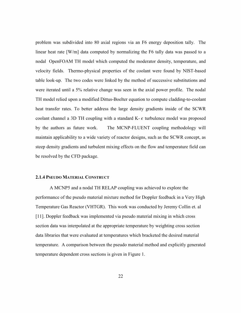
2.1.4 PSEUDO MATERIAL CONSTRUCT
A MCNP5 and a nodal TH RELAP coupling was achieved to explore the
performance of the pseudo material mixture method for Doppler feedback in a Very High
Temperature Gas Reactor (VHTGR). This work was conducted by Jeremy Collin et. al
[11]. Doppler feedback was implemented via pseudo material mixing in which cross
section data was interpolated at the appropriate temperature by weighting cross section
data libraries that were evaluated at temperatures which bracketed the desired material
temperature. A comparison between the pseudo material method and explicitly generated
temperature dependent cross sections is given in Figure 1.

23
Figure 1: Comparison of the pseudo material mixing method with explicit Doppler
broadened cross section data on the neutron multiplication factor of a
VHTGR fuel pin. Reproduced from [11].
In this figure, the pseudo material mixing procedure is shown to give similar
results when compared to explicitly Doppler broadened cross section treatment. In
Collin’s implementation, the energy dependent microscopic cross sections are weighted
by the square-root temperature distance to the bounding temperatures. This weighting
scheme is consistent with the energy dependence of the Doppler broadened cross section
resonance integral. This method of cross section interpolation is adopted in the present
work. An explanation of the pseudo material mixing procedure is given in chapter 3.
2.1.5 COUPLED NEUTRONICS AND TH SIMULATIONS USING MCNP AND FLUENT
Work conducted at the University of Illinois, Urbana by Jianwei Hu and Rizwan-
uddin resulted in another coupling of MCNP5 to ANSYS FLUENT [12]. FLUENT’s

24
User-Defined-Function (UDF) capability allowed volumetric energy deposition data from
MCNP to be read into the CFD mesh. The mesh used in FLUENT was identical to the
F6 heating mesh in MCNP, allowing a 0th
order interpolation scheme to map volumetric
heating rates to the FLUENT mesh. Doppler broadening feedback was implemented by
nearest neighbor cross section interpolation with a temperature resolution of 100K.
Figure 2: Coarse 4x4x4 cell meshed
used in [12].
Figure 3: Volumetric energy deposition rates at
the z+ midplane. [12]
Shown in figures Figure 2 andFigure 3, implementation of the coupling
methodology was limited to the relatively simple 2D slab geometry coarsely discretized
by as 4x4 grid. This geometry does not give rise to many of the coupling challenges
encountered in full scale reactor physics calculations. Regardless, the work proved the
feasibility of using user defined C functions (UDFs) to ease field data transfer and
interpolation in FLUENT and implementing an external Perl wrapping script of MCNP
and ANSYS FLUENT.

25
2.1.6 MCNP5 – STAR-CCM+ COUPLING
A masters project conducted by Jefferey Cardoni at the University of Illinois at
Urbana-Champaign demonstrated a 3D coupling of MCNP5 and STAR-CCM+ [13].
Identical to the aforementioned coupling methodologies, the method of successive
substitutions iteration scheme was employed to solve to coupled problem.
The energy deposition field was discretized using an extremely large number of
traditional MCNP cells each with an associated F7 fission heating rate tally. 7,489
individual elements were used in a single pin case and 67,401 elements in a 3x3 pin case.
The MCNP input deck was generated algorithmically. Each cell was assigned a unique
ID, such that it could be mated with its TH cell counterpart.
Figure 4: STAR-CCM+ mesh (left). MCNP cells (right). Reproduced from [13].
Shown in Figure 4, the TH mesh was constructed such that a high degree of mesh
parity was obtained, though an exact match was not pursued. A nearest neighbor
interpolation scheme was used to map volumetric heat data from MCNP to STAR-CCM.
A Perl script linked each MCNP cell with a TH cell according to a minimum distance
criterion. Neutron and gamma heating in the coolant was neglected as ~97% of the
26
recoverable fission energy is claimed to be deposited in the fuel. Therefore the author did
not tally heating rates inside the moderator or cladding.
The TH mesh was not refined near the cladding-coolant interface. In order to
obtain a convective heat transfer rate, law-of-the-wall approximations were employed by
STAR-CCM at the interface to approximate the temperature and velocity gradients at the
wall. This decision was likely made to conserve computational resources while
demonstrating the initial functionality of the coupling. Furthermore, allowing flexible
mesh cell spacing would require modification of the Perl script responsible for mesh
generation and cell linking. To avoid complications and geometric inflexibility induced
by cell-to-cell linking, the method employed in this thesis will instead employ a volume
averaging scheme to map the finely resolved TH field data into larger MCNP cells.
2.1.7 COUPLED CFD AND MOC SIMULATIONS
Work performed by a Michigan Ann Arbor, Oak Ridge National Lab and
Westinghouse Electric Company consortium coupled a method of characteristics
transport code with a CFD thermal hydraulics code to obtain high resolution pin power
and velocity profiles for a 3x3 PWR lattice geometry [14]. This work fulfilled the CASL
milestone: “Apply a baseline transport (DeCART) and CFD (STAR-CCM+) capability
with loose coupling to a PWR 3x3 fuel pin with a spacer grid to demonstrate feedback
coupling” in the Advanced Modeling Applications (AMA) CASL Focus Area (FA). This
work is distinguished from other coupling attempts because the spacer grid present in the
assembly is resolved explicitly in the TH mesh, however the spacer grid is homogenized
in the neutronics model.
27
The method of successive substitutions was used to couple the two codes
together. Convergence was obtained when the L1 neutron multiplication factor norm and
the L2 fission source distribution and temperature distribution norms reached a
satisfactorily stationary value.
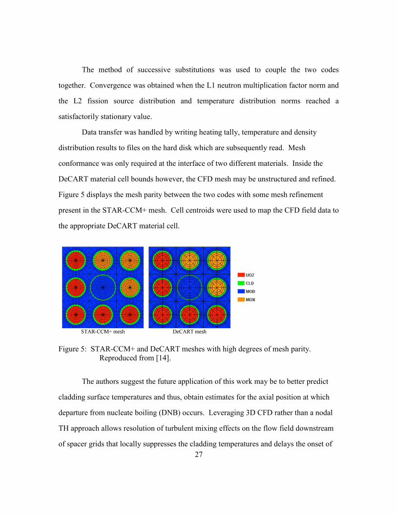
Data transfer was handled by writing heating tally, temperature and density
distribution results to files on the hard disk which are subsequently read. Mesh
conformance was only required at the interface of two different materials. Inside the
DeCART material cell bounds however, the CFD mesh may be unstructured and refined.
Figure 5 displays the mesh parity between the two codes with some mesh refinement
present in the STAR-CCM+ mesh. Cell centroids were used to map the CFD field data to
the appropriate DeCART material cell.
Figure 5: STAR-CCM+ and DeCART meshes with high degrees of mesh parity.
Reproduced from [14].
The authors suggest the future application of this work may be to better predict
cladding surface temperatures and thus, obtain estimates for the axial position at which
departure from nucleate boiling (DNB) occurs. Leveraging 3D CFD rather than a nodal
TH approach allows resolution of turbulent mixing effects on the flow field downstream
of spacer grids that locally suppresses the cladding temperatures and delays the onset of

28
DNB. Subcooled boiling rates are important to accurately predict when studying CRUD
deposition rates and TH reactor safety margins [35].
2.1.8 COUPLED CFD AND MONTE CARLO SIMULATIONS
Preceding the work of the aforementioned DeCART/STAR-CCM+ coupling, V.
Seker et. al. completed a loose coupling between MCNP5, NJOY, and STAR-CCM+
which was named McSTAR [15]. Doppler feedback was handled by interpolating pre-
computed cross sections in each material region. Discretiztion of the fuel and moderator
in MCNP was accomplished using standard MCNP cells depicted in an overhead view in
Figure 6. The cell geometry generation procedure was scripted to simplify the
construction of PWR lattice geometries.
Figure 6: MCNP5 cell based geometry discreteization. Reproduced from [15].
To demonstrate the preliminary MCNP and STAR coupling capability the
solution produced by McSTAR was compared against a coupled DeCART/STAR
simulation for a 3x3 pin problem. A maximum pin power difference of 4% was reported
between the DeCART and MCNP coupled calculations. The authors reported that 300
active cycles were utilized per outer iteration with 5e5 neutrons histories simulated per

29
cycle. A total of 12 outer Picard iterations were performed requiring approximately 100
hours of simulation time on 120 cores.
The authors recognized that due to large computation times required to reduce
uncertainty in the estimated parameters Monte Carlo neutron transport was not expected
to displace deterministic transport for large scale core design and optimization
applications. Instead, the proposed targeted use case for the MCNP5-STAR-CCM+ was
to provide an audit tool for simple, few-pin coupled PWR problems. The MCNP-
FLUENT coupling is expected to be limited to similar small-geometry applications.
2.1.9 LITERATURE REVIEW CONCLUSION
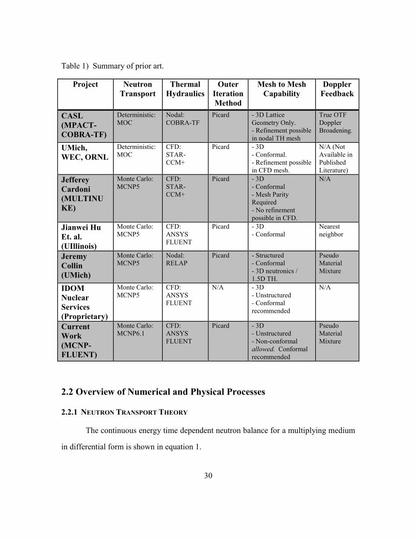
A weakness present in the majority of the coupling methods, with the notable
exception of IDOM Nuclear Services’ implementation of an MCNPX-Fluent coupling,
was the requirement for conformal CFD and heating tally meshes. This weakness is
present to reduce mesh to mesh interpolation algorithmic complexity and to reduce the
computational requirement associated with estimating volume integrals and/or computing
a mapping matrix required for a generic mesh to mesh coupling scheme. Furthermore,
enforcing mesh conformity alleviates concerns of interpolation error. A review of prior
art is presented in Table 1.
30
Table 1) Summary of prior art.
Project Neutron
Transport
Thermal
Hydraulics
Outer
Iteration
Method
Mesh to Mesh
Capability
Doppler
Feedback
CASL
(MPACT-
COBRA-TF)
Deterministic:
MOC
Nodal:
COBRA-TF
Picard - 3D Lattice
Geometry Only.
- Refinement possible
in nodal TH mesh
True OTF
Doppler
Broadening.
UMich,
WEC, ORNL
Deterministic:
MOC
CFD:
STAR-
CCM+
Picard - 3D
- Conformal.
- Refinement possible
in CFD mesh.
N/A (Not
Available in
Published
Literature)
Jefferey
Cardoni
(MULTINU
KE)
Monte Carlo:
MCNP5
CFD:
STAR-
CCM+
Picard - 3D
- Conformal
- Mesh Parity
Required
- No refinement
possible in CFD.
N/A
Jianwei Hu
Et. al.
(UIllinois)
Monte Carlo:
MCNP5
CFD:
ANSYS
FLUENT
Picard - 3D
- Conformal
Nearest
neighbor
Jeremy
Collin
(UMich)
Monte Carlo:
MCNP5
Nodal:
RELAP
Picard - Structured
- Conformal
- 3D neutronics /
1.5D TH.
Pseudo
Material
Mixture
IDOM
Nuclear
Services
(Proprietary)
Monte Carlo:
MCNP5
CFD:
ANSYS
FLUENT
N/A - 3D
- Unstructured
- Conformal
recommended
N/A
Current
Work
(MCNP-
FLUENT)
Monte Carlo:
MCNP6.1
CFD:
ANSYS
FLUENT
Picard - 3D
- Unstructured
- Non-conformal
allowed. Conformal
recommended
Pseudo
Material
Mixture
2.2 Overview of Numerical and Physical Processes
2.2.1 NEUTRON TRANSPORT THEORY
The continuous energy time dependent neutron balance for a multiplying medium
in differential form is shown in equation 1.

31
1
v
∂𝜓
∂t− 𝛀 ⋅ ∇(𝜓) − Σ𝑡(𝑥, 𝐸)𝜓 + ∫ ∫ Σ𝑠(𝑥, 𝛀′ ⋅ 𝛀, 𝐸′ → 𝐸)
4𝜋
0
∞
0
𝜓𝑑𝛀′𝑑𝐸′
+χ(x, E)
4𝜋∫ ∫ 𝜈(𝑥, 𝐸′)Σ𝑓(𝑥, 𝐸′)𝜓𝑑𝛀′𝑑𝐸′
4𝜋
0
∞
0
+𝑆
4𝜋= 0 (1)
𝜓 = 𝜓(𝑥, 𝛀, 𝐸)
The first term represents the streaming of neutrons through a point in space. The
second term is the net neutron removal rate when considering all possible neutron
interactions. The third term accounts for scattering events which redistribute the neutrons
in energy and direction. The fourth term represents neutron born in fission events. The
final term includes non-fission included neutron sources. All neutrons born from fission
are assumed to be promptly emitted. No delayed neutron contribution to the rate
equation is considered for simplicity.
In the problem of interest in this thesis, in which a fissile material provides
neutron multiplication and no fixed source is present, the time derivative may be
eliminated by scaling the neutron production rate from fission by a factor of 1/𝑘.
𝛀 ⋅ ∇(𝜓) − Σ𝑡(𝑥, 𝐸)𝜓 + ∫ ∫ Σ𝑠(𝑥, 𝛀′ ⋅ 𝛀, 𝐸′ → 𝐸)4𝜋
0
∞
0
𝜓𝑑𝛀′𝑑𝐸′
+χ(x, E)
𝑘4𝜋∫ ∫ 𝜈(𝑥, 𝐸′)Σ𝑓(𝑥, 𝐸′)𝜓𝑑𝛀′𝑑𝐸′
4𝜋
0
∞
0
= 0
The inclusion of the neutron multiplication factor results in a pseudo steady state
neutron balance. The pseudo steady state multiplying medium transport equation may be
discretized in energy, producing a set of coupled equations known as the multigroup
transport equations. The multigroup transport equation may be represented concisely in
matrix form:
𝑯𝜓 =1
𝑘χ𝑓𝑇 ∫ 𝑑𝛀𝜓
4𝜋

32
The multigroup transport operator H acts on the multigroup neutron flux vector 𝜓
to redistribute neutrons in energy due collisions and to remove neutrons due to
absorptions:
𝑯𝑔𝑔′ = 𝛿𝑔𝑔′[𝛀 ⋅ ∇ + Σ𝑡(𝑥)]𝑔𝑔 + ∫ Σ𝑠𝑔𝑔′(𝑥, 𝛀′ ⋅ 𝛀)
4𝜋
0
𝑑𝛀
The discrete energy fission probability distribution and fission multiplicity row
vectors are defined respectively:
χ = {χg1, … ΧgN
}
𝑓𝑇 = {νΣfg1, … νΣfgN
}𝑇
For compactness it is useful to define a neutron production rate vector:
𝐹(𝑥) = 𝑓𝑇 ∫ 𝑑𝛀𝜓4𝜋
Multiplying by the inverse of 𝑯 and operating on 𝜓 on both sides of transport
equation with 𝑓𝑇 ∫ 𝑑𝛀4𝜋
yields:
𝑘𝑓𝑇 ∫ 𝑑𝛀𝜓4𝜋
= χ𝑓𝑇 ∫ 𝑑𝛀4𝜋
𝐇−1𝑓𝑇 ∫ 𝑑𝛀𝜓4𝜋
Using the definition of 𝐹(𝑥) we obtain:
𝑘𝐹 = χ𝑓𝑇 ∫ 𝑑𝛀4𝜋
𝐇−1𝐹
𝐀 = χ𝑓𝑇 ∫ 𝑑𝛀4𝜋
𝐇−1
We arrive at a k-eigenvalue problem:
𝑘𝐹 = 𝑨𝐹
This equation may be numerically solved by the method of power iteration [16].
The power iterations are carried out by repeatedly applying the operator 𝑨 to an initial
guess for the angle integrated multigroup fission distribution shape, 𝐹0. At each iteration
𝑖, the vector is updated according to:

33
𝐹𝑛 = ∏ 𝑘𝑖−1
𝑖=𝑁
𝑖=0
𝑨𝑛𝐹𝑜
And the neutron multiplication factor is updated according to:
𝑘𝑖+1 =∫ 𝐹𝑖+1 𝑑𝑉
(1/𝑘𝑖) ∫ 𝐹𝑖 𝑑𝑉=
∫ 𝑨𝐹𝑖 𝑑𝑉
∫ 𝐹𝑖 𝑑𝑉
Where V is the reactor volume.
Assume there are 𝑙 eigenvalues and eigenvectors each representing a possible solution to
the eigenvalue problem shown in equation 2.
𝑨𝐹𝑙 = 𝜆𝑙𝐹𝑙
(2)
The initial guess 𝐹0 is some linear combination of the solution eigenvectors:
𝐹0 = ∑ 𝛼𝑙𝐹𝑙
𝑙
Applying A a total of n times produces:
𝑨𝑛𝐹𝑜 = ∑ 𝜆𝑙𝑛𝛼𝑙𝐹𝑙
𝑙
= 𝛼1𝜆1𝑛𝐹1 + ∑ 𝜆𝑙
𝑛𝛼𝑙𝐹𝑙
𝑙>1
(3)
Assuming atleast one positive real eigenvalue exists, and there are no duplicate
eigenvalues (all solution eigenvectors are linearly independent) then there is an ordered
sequence of eigenvalues that satisfies 𝜆1 > 𝜆2 > 𝜆3 …. According to equation 3, as n
becomes large the largest eigenvalue and corresponding eigenvector will dominate the
fission source distribution, 𝐹. This eigenvector is termed the fundamental harmonic of
the fission source distribution. The rate at which a stationary solution is achieved by
power iteration is dependent on the ratio 𝜆2 𝜆1⁄ . If this ratio is small then (𝜆𝑙 𝜆1⁄ )𝑛 tends
to 0 in relatively few power iterations. It can be shown that in cases where the root-
mean-squared distance a neutron travels before causing a fission is much smaller than the
dimensions over which the fissile material is spread gives rise to slow convergence [16].
34
Non fundamental mode eigenvectors may persist in the solution estimate over many
power iterations. This case has the potential to arise in PWR criticality calculations as
the axial and radial dimensions are large.
Briefly, there are a variety of acceleration methods available to combat slow
convergence to the fundamental mode when using power iteration to solve the k-
eigenvalue problem. The Coarse-Mesh Finite Difference (CMFD) technique is
commonly employed to damp the higher harmonics of the fission source distribution by
rebalancing the neutron population in space according to lower order approximations to
the neutron transport equation. This method has shown to be an effective means to
accelerate a variety of transport codes, including MPACT [7, 8]. Despite their
attractiveness, acceleration techniques for k-eigenvalue power iterations are not a focus
of this thesis however, incorporating a CMFD acceleration step into the MCNP KCODE
solution updates is an active area of research [17].
For every power iteration the inverse of the multigroup transport operator H must
be computed. This operation often requires iterative procedure such as the Gauss-Seidel
method to be invoked. From the perspective of MCNP, the inversion of the transport
operator is carried out implicitly by simulating many particle histories, though there is no
exact analogy to the matrix inversion operation in Monte Carlo transport methodology.
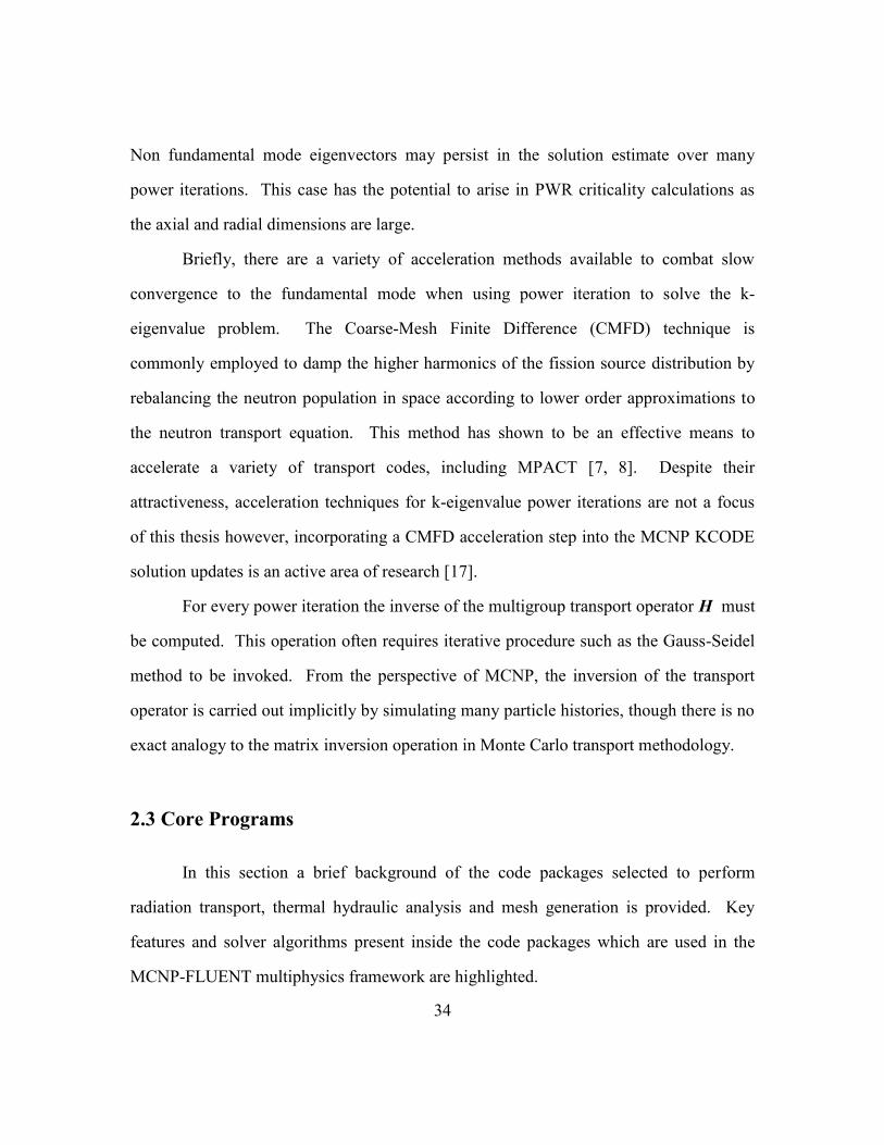
2.3 Core Programs
In this section a brief background of the code packages selected to perform
radiation transport, thermal hydraulic analysis and mesh generation is provided. Key
features and solver algorithms present inside the code packages which are used in the
MCNP-FLUENT multiphysics framework are highlighted.

35
2.3.1 NEUTRON TRANSPORT: MCNP6.1
The Monte Carlo N-Particle transport package MCNP v.6.1 is leveraged for
radiation transport [18]. This package is capable of Continuous Energy (CE) neutron and
photon transport. Monte Carlo methods in radiation transport reduce the number of
simplifications applied to the physics of simulation of particle transport at the expense of
providing only an approximate solution to the transport equation. The simulated
particles’ aggregate behavior solves the transport equation exactly in the limit as the
number of simulated particle histories approaches infinity. Interaction probabilities are
derived from experimentally obtained nuclear physics cross section data when available.
User generated cross section data can be supplied in the ACE format via the cross section
processing tool NJOY.
MCNP will be used in the KCODE mode to solve the k-eigenvalue problem
presented in equation (2). In this mode, an initial guess for the spatial neutron fission
source distribution is provided. With each simulated neutron generation, an improved
estimate for the true fission source distribution is obtained by releasing neutrons from the
previous source locations, simulating their lifetimes and finally updating the source
distribution according to the updated fission event spatial distribution. Given enough
neutron generations are simulated, the fission source distribution converges to the true
shape. The solution method is essentially the method of power iteration as described in
section 2.2.1 Neutron Transport Theory, with similar drawbacks of slow convergence for
large, loosely coupled multiplying geometries.
MCNP allows the problem domain to be spatially discretized for reaction rate
tallying enabling the end user to obtain an estimate for the local energy deposition inside
a given volume embedded in the model, for example. With the release of v6.0, MCNP
gained the capability to import unstructured meshes supplied in the ABAQUS ASCII

36
mesh file format. The unstructured mesh can be used to define a mesh tally, though the
output scalar field data is written in the EEOUT file format which significantly differs
from a MCTAL file. Detailed information on the EEOUT format may be found in the
MCNP unstructured mesh manual [19]. In addition, user specified regions in the
unstructured mesh can be treated as traditional MCNP cells in which material
composition and temperature may be assigned. This capability enables highly complex
geometry involving multiple materials to be easily defined and meshed. Before the
advent of this capability, individual MCNP macrobodies could have been combined to
form a mesh using traditional cell based reaction rate tallies. Other coupling
methodologies relied upon traditional structured mesh tallies superimposed over
constructive solid geometry cells.
When coupling equation 1 with thermal and fluid transport PDEs as is the case in
reactor calculation of interest, the energy deposition rate due to fission events must be
computed. In MCNP an F6 tally can be used to compute the local energy deposition due
to all particle iterations. The F6 tally estimates the integral given by equation 4 [18].
𝐹6 =𝑁
𝑉𝜌∭ 𝐻(𝐸)𝜙(𝑥, 𝑉, 𝑡)𝑑𝑉𝑑𝑡𝑑𝐸
𝑉,𝑡,𝐸
(4)
Where V is the volume of the F6 tally cell, 𝜌 is the mass density, N is the atomic density,
E is energy, and t is time. The heating response function H(E) is strongly dependent on
the microscopic fission cross section in instances when energy deposition due to fission
events is of primary interest with other minor contributions from neutron collision and
gamma heating. 𝜙 is the angle integrated scalar flux. The F6 tally produces results in
[𝑀𝑒𝑉/𝑔𝑟𝑎𝑚 𝑠𝑜𝑢𝑟𝑐𝑒 𝑝𝑎𝑟𝑡𝑖𝑐𝑙𝑒⁄ ] [18]. To provide a volumetric heating rate to a coupled
thermal hydraulic code requires scaling the raw F6 tally by the mass density of the

37
material and by a scalar quantity 𝐶𝑖 determined by the power normalization given in
equation 5:
𝑄𝑖 = 𝐹6𝜌𝑖𝐶𝑖 [𝑊𝑎𝑡𝑡𝑠/𝑐𝑚3]
𝑅𝑒𝑎𝑐𝑡𝑜𝑟 𝑃𝑜𝑤𝑒𝑟 = 𝑄𝑡𝑜𝑡 = ∑ 𝑄𝑖𝑉𝑖
𝑐𝑒𝑙𝑙𝑠
(5)
Where the scalar 𝐶𝑖 has units of [1/s].
2.3.2 THERMAL HYDRAULICS: ANSYS FLUENT
The following capabilities were desired from the TH modeling software:
Ease of field data transfer to and from the simulation package
Heat transport in solid bodies
Buoyancy driven flow
Arbitrarily complex geometry
Ability to include turbulence effects in a Buoyancy driven flow model
ANSYS FLUENT v. 14.0 was adopted as the TH code of choice. ANSYS
FLUENT is capable of performing all of the tasks listed above [20]. This package is
capable of conjugate heat transfer and provides built in methods to read and write field-
data to ASCII files. The package contains a multitude of turbulence models to choose
from which are compatible with buoyancy driven flow models. FLUENT is a finite
volume based Computational Fluid Dynamics (CFD) package. Multiple discretization
schemes and solution methodologies are available to the user. The Simi-Implicit Method
for Pressure Linked Equations (SIMPLE) pressure-velocity coupling scheme will be
employed in this thesis. Overviews of the finite volume discretization method for PDEs
and the SIMPLE solution algorithm may be found in [21].
38
FLUENT’s conjugate heat transfer capability allows the energy balances written
for cells inside the solid regions in the problem to be directly coupled with the energy
balances equations in the fluid portions of the mesh. This results in only one matrix
equation for the thermal energy balance to be solved per TH iteration. This reduces
overall computation time as it alleviates the need for a separate solid heat transport solver
and an additional solution coupling procedure.
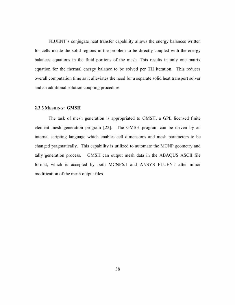
2.3.3 MESHING: GMSH
The task of mesh generation is appropriated to GMSH, a GPL licensed finite
element mesh generation program [22]. The GMSH program can be driven by an
internal scripting language which enables cell dimensions and mesh parameters to be
changed pragmatically. This capability is utilized to automate the MCNP geometry and
tally generation process. GMSH can output mesh data in the ABAQUS ASCII file
format, which is accepted by both MCNP6.1 and ANSYS FLUENT after minor
modification of the mesh output files.
39
CHAPTER 3
Methodology
The coupled physics framework simultaneously solves for multiple physical
fields, in this case flow velocity, temperature, energy deposition rate, and neutron flux. It
does so by repeatedly passing information between dedicated solvers which
independently handle the neutron transport and thermal hydraulic physics. The codes are
linked by the method of successive substitutions, or a Picard Iteration scheme which is
discussed in section 3.1.6 Picard Iterations and Convergence and is referred to as the
outer iteration scheme. This chapter describes the outer iteration scheme as well as the
implementation of the dedicated solvers which it brings together.
3.1 COUPLING PROCEDURE
Figure 7 illustrates the iterative multiphysics coupling procedure. The problem
geometry must first be defined, meshes constructed for FLUENT and MCNP, and
temperature dependent cross section data generated before the automated outer Picard
iterations begin. Scripts developed in the Python language handle all data transfer to and
from MCNP and FLUENT in addition to automating the generation of MCNP input
decks and FLUENT journal files.

40
Set Initial MCNP materials
and BCs
Define TH BCs & Allocate memory
for custom scalar field
MCNP deck generator
Problem Setup
Automated
Iterations
Gen NJOY ACE Libs
aaANSYS
Fluent
MCNP
Pseudo Material Mixer
Scalar Field Parser
END ITERATIONS
Parse MCNP F6 Tally
Normalize Heat source
Construct Finished
Journal FileCompute Cell Densities &
Temperatures
Energy Deposition Tally
Density &
Temperature
Fields
Specify Geometry
GMSH Mesh Gen
FE Meshes
CONVERGED?
Iteration = 0
Iteration++
Figure 7: MCNP-FLUENT coupling procedure overview.
Following the problem setup, the automated iteration loop is initiated, first,
computing the temperature and density in each component of the MCNP problem
geometry according to the initial conditions provided in the problem setup. MCNP is
responsible for computing the energy deposition scalar field. The energy deposition data
is passed to an preprocessor which applies a normalization to the energy deposition field
such that the total thermal power produced the be problem domain is equivalent to a user
set value.
Given boundary conditions and a volumetric heat source distribution, ANSYS
FLUENT approximately solves a coupled energy, mass, and momentum balance
throughout the problem domain to obtain solution field variables – temperature and
density – which feed back to the neutron transport calculations. The TH solution data is

41
passed into interpolation routines which compute the temperature, density and material
composition in each MCNP cell.
After MCNP is executed (for the second time), scaled residuals are computed and
checked against a converge tolerance. The process is repeated until the convergence
criteria are met or a maximum number of outer iterations are performed. The remainder
of this section explains each step of the process in detail.
3.1.1 Geometry Specification and Mesh Generation
The fundamental geometric component in MCNP is a cell. Traditionally, an
MCNP cell is defined by Boolean combinations of spatial regions. This is the
constructive solid geometry (CSG) approach to geometry specification. The current work
departs from the use of CSG techniques in favor of the flexible UM geometry
construction paradigm. To maintain consistency with standard MCNP UM terminology,
geometric components used to construct the problem are referred to as UM parts. A
variety of parts typically employed to build PWR lattice geometries are provided in
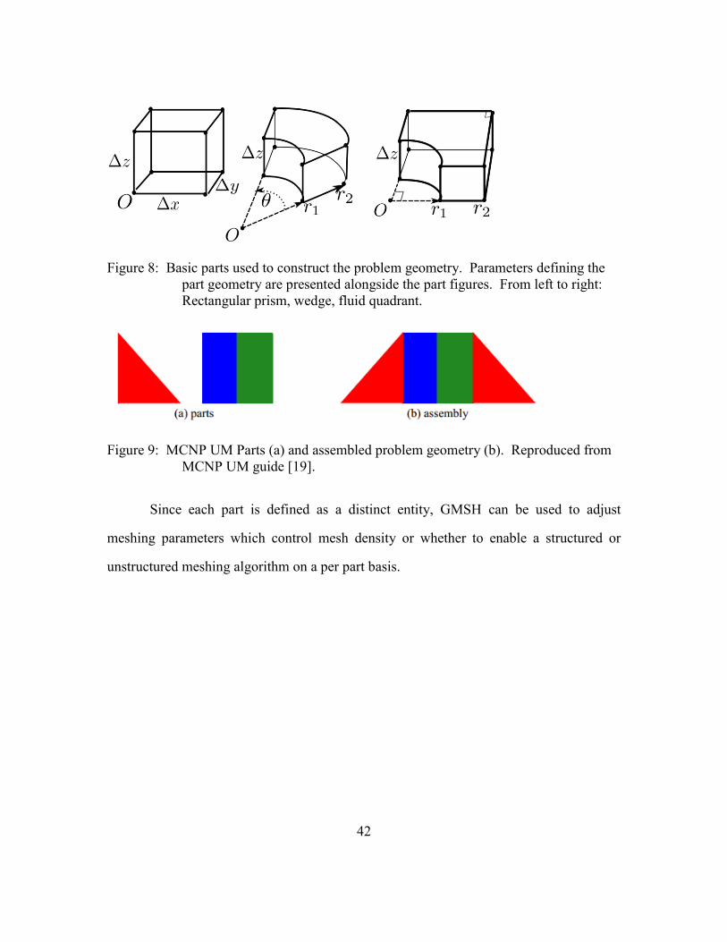
Figure 8. Figure 9 shows that assemblies are constructed from a collection of simple
parts. Each part is located in Cartesian space by specifying the part origin. In addition,
each part contains unique parameters which fully define its geometry.
42
Figure 8: Basic parts used to construct the problem geometry. Parameters defining the
part geometry are presented alongside the part figures. From left to right:
Rectangular prism, wedge, fluid quadrant.
Figure 9: MCNP UM Parts (a) and assembled problem geometry (b). Reproduced from
MCNP UM guide [19].
Since each part is defined as a distinct entity, GMSH can be used to adjust
meshing parameters which control mesh density or whether to enable a structured or
unstructured meshing algorithm on a per part basis.

43
Figure 10: A collection of rectangular prism parts constructed into a single assembly.
The underlying mesh is visible in each part.
MCNP UM parts are used define pseudo-cells in the MCNP input. Pseudo-cells
are analogous to traditional MCNP cells with minor restrictions that are irrelevant to this
work. Example input cards utilizing the MCNP unstructured meshing capability may be
found in the MCNP UM users guide [19]. Each pseudo-cell is associated with unique
material, density, and temperature information so that the cell properties may be updated
throughout the iterative solution procedure. Henceforth the prefix “pseudo” will be
dropped when referring to a region of space inside the MCNP geometry which is
assigned unique material and temperature information. MCNP UM pseudo-cell’s will be
referred to simply as cells. In addition to material properties, a Boolean is assigned to
each cell indicating whether it contains a multiplying medium so that the flagged cell can
be specified as a source region inside MCNP using the special VOLUMER keyword on
the SDEF card.
A plane wall assembly that is ready for MCNP or FLUENT import is shown in
Figure 10. MCNP pseudo-cells are differentiated by color, and the unstructured mesh is
shown as yellow lines. The mesh can be used as an F6 heating mesh tally definition
within MCNP. The same mesh can be imported into ANSYS FLUENT using the built in

44
ABAQUS mesh import functionality. In contrast to constructive solid geometry (CSG)
MCNP specification, implementation of the unstructured mesh geometric representation
technique allows one to obtain identical meshes in both MCNP and ANSYS FLUENT,
helping to eliminate grid-to-grid interpolation error issues. This is a primary benefit of
taking advantage of MCNP6.1 unstructured mesh support for multiphysics coupling
applications.
3.1.2 MCNP
All UM pseudo-cells are collected into a single assembly which is placed into a
conventional MCNP container cell. The container cell is a traditional MCNP
constructive geometry cell which is used as the problem’s bounding box. Boundary
conditions are specified on the container cell faces and particle importances are set to null
outside of the container.
Figure 11: Unstructured mesh embeded in a traditional CSG container cell. Cells
(distinct material regions) are differentiated by color.

45
Figure 11 displays the unstructured mesh placed within the container cell. In the
figure pseudo-cells are denoted by color. Each cell is associated with a corresponding
material definition in the MCNP input deck. Since each cell is tagged with a material
name, and the density of the material inside the cell is known, the appropriate material
and isotopic vector can be selected from a global inventory dictionary, e.g. a cell with a
material name “lwtr” will be assigned hydrogen and oxygen isotopes in their proper
proportions.
In each cell’s material definition, MCNP requires isotopes to be associated with
continuous energy cross section libraries. Assigning the correct cross section library to
each isotope inside a given cell depends upon the cell temperature. The cell average
temperature is computed by integrating the temperature scalar field data provided by
FLUENT simulation results inside of the cell in question. The procedure is discussed in
detail in section 3.1.3. Given the cell temperature, an approximate method known as
pseudo material mixing is used to handle Doppler feedback. Interpolation of the cross
section libraries bracketing the average cell temperature is performed. Cross section data
libraries are weighted by the relative distance to bounding cross section temperature
abscissa. This pseudo material mixing procedure is discussed in section 3.1.4.
An F6 heating tally is generated using the collective assembly mesh. The F6 tally
measures the energy deposited per unit mass due to locally deposited fission gammas,
and from neutron collisions and absorptions [18]. The raw F6 heating tally is normalized
according to equation 6 to obtain volumetric heating rates.
𝐸𝑖 =𝐶𝜌𝑖𝐹𝑖𝑉𝑖
∑ 𝜌𝑖𝐹𝑖𝑉𝑖𝑁𝑖=0
(6)
46
Where 𝑖 is the cell index, E is the total energy deposition in [Watts]. 𝐹 is the raw
F6 tally values [eV/gram/source particle], 𝜌 is the volume averaged material density in
the cell, and 𝐸𝑖/𝑉𝑖 is the volumetric heating rate inside a given MCNP mesh element. 𝐶
is a user defined scaling parameter with units of [Watts] that scales the energy deposition
tally to yield the specified amount of power when integrated over the entire problem.
It should be noted that a MCNP “continue run” operation is not permitted when
material compositions change within the problem between outer iterations due to the
pseudo material mixing procedure. Following the first Picard iteration, the previous
fission source distribution is available for use as the fission source initial guess in the
current iteration. This is accomplished with the MCNP fission source import command
line argument accompanied by a SRCTPE file [18].
3.1.3 Grid to Grid Interpolation
Field data must be exchanged between the MCNP and the FLUENT meshes. The
resolution at which material, temperature, and density information is tracked within
MCNP is only cell-resolved. Within FLUENT, temperature and density scalar fields are
comparatively finely resolved. The CFD temperature and density fields are supported at
the CFD mesh element centroids. An interpolation scheme must be employed to map the
finely resolved temperature and density scalar field information onto the coarsely
resolved Cell-based geometry description in MCNP.

47
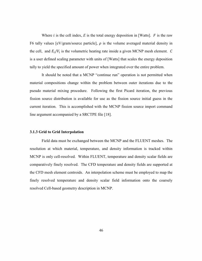
Figure 12: Discrete temperature field data points superimposed on an MCNP cell.
Discrete temperature and density field data is passed from the FLUENT
computation to MCNP. In the following example, the temperature field data is
considered. In Figure 12 an MCNP cell is presented with origin O{x0, y0, z0} alongside
discrete temperature data as received from a mesh-cell centered FLUENT data set, shown
as 𝑇𝑖. Red points indicated data which lie inside of the cell, blue data points lay outside
of the cell. A piecewise continuous linear interpolating function, 𝜓, is constructed upon
the discrete temperature data set. In equation (7 this function is integrated over the cell
volume to obtain an average temperature within the cell. The integration limits and cell
volume are easily determined from the cell parameters (𝑂, Δ𝑥, Δ𝑦, Δ𝑧) in the case of a
rectangular prism cell. In the case of more complex cell geometry the volume integral in
equation (7 is not trivial to compute.
𝑇𝑐𝑒𝑙𝑙 =
1
𝑉𝑐𝑒𝑙𝑙∫ 𝜓𝑑𝑉
𝑉
(7)
This piecewise linear interpolation procedure is particularly susceptible to
interpolation errors when large second derivatives exist in the field data. Refining the
48
number of cells in the MCNP domain reduces interpolation error at the expense of
computing time to resolve the field at a greater fidelity.
For MCNP cells of arbitrary shape a novel procedure was developed to compute
equation 7. Consider a single UM part in the MCNP geometry, for example a quarter-
cylindrical ring shaped region in the fuel. The underlying finite element mesh generated
by GMSH is comprised of simple geometric elements (arbitrary shaped hexahedron)
which are guaranteed to be convex. A 2D representation of a hexahedral element is
provided in Figure 13.
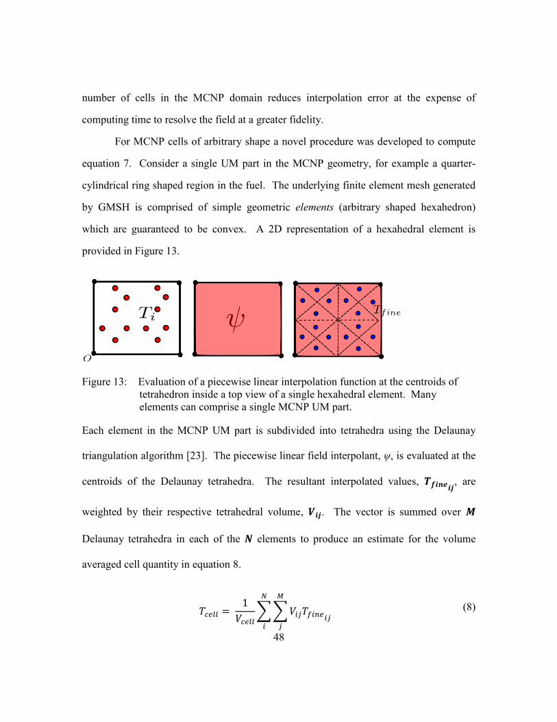
Figure 13: Evaluation of a piecewise linear interpolation function at the centroids of
tetrahedron inside a top view of a single hexahedral element. Many
elements can comprise a single MCNP UM part.
Each element in the MCNP UM part is subdivided into tetrahedra using the Delaunay
triangulation algorithm [23]. The piecewise linear field interpolant, ψ, is evaluated at the
centroids of the Delaunay tetrahedra. The resultant interpolated values, 𝑻𝒇𝒊𝒏𝒆𝒊𝒋, are
weighted by their respective tetrahedral volume, 𝑽𝒊𝒋. The vector is summed over 𝑴
Delaunay tetrahedra in each of the 𝑵 elements to produce an estimate for the volume
averaged cell quantity in equation 8.
𝑇𝑐𝑒𝑙𝑙 = 1
𝑉𝑐𝑒𝑙𝑙∑ ∑ 𝑉𝑖𝑗𝑇𝑓𝑖𝑛𝑒𝑖𝑗
𝑀
𝑗
𝑁
𝑖
(8)

49
This volume integral estimation method is applicable regardless of the FLUENT
mesh density, shape of the MCNP parts, mesh scheme implemented in each MCNP part,
or how few MCNP parts make up the problem geometry.
3.1.4 Doppler Feedback
As a component of problem setup, the nuclear data processing code, NJOY, is
executed to obtain ACE formatted Doppler broadened cross sections for every isotope
present in the problem at 50K intervals [24]. The fuel material temperatures considered
range from 300K to 1400K. Cross sections for the isotopes present exclusively inside the
moderator are generated from 300K to 700K. Equation (9 illustrates that cross sections
for the isotopes in a cell are weighted by the square root temperature distance to
bounding cross section temperature abscissa. This is consistent with the temperature
dependence of the Doppler broadened resonance integral [13, 25].
Σ𝑐𝑒𝑙𝑙 = 𝑤𝑐Σ𝑐 + (1 − 𝑤𝑐)Σℎ
(9)
With weight:
𝑤𝑐 = (√𝑇ℎ − √𝑇𝑐𝑒𝑙𝑙
√𝑇ℎ − √𝑇𝑐
)
Tc &Th are the bounding hot and cold temperatures for which Doppler-broadened
XS data exists. Σ represents the macroscopic cross section of the mixed material in a
50
cell. Expanding macroscopic cross sections in equation 10 exposes the number density of
the jth
isotope inside the mixture:
Σ𝑐𝑒𝑙𝑙 = ∑ 𝑁𝑗[𝑤𝑐(σj)𝑐 + (1 − 𝑤𝑐)(σj)ℎ]
𝑗
(10)
The weighted isotopes, 𝑤𝑐𝑁𝑗 and 𝑤ℎ𝑁𝑗, correspond to bounding lower and upper
cross sections (σj)𝑐 and (σj)ℎ respectively. The microscopic cross sections, σj, are
continuous functions of energy. According the MCNP material specification format,
cross sections for the same isotope at different temperatures may be uniquely identified
by library suffix tags. The appropriate cross section libraries can thus be selected from a
pre-generated list and the number densities can be appropriately weighted before being
written to a MCNP material card.
3.1.5 ANSYS FLUENT
After a mesh is imported into FLUENT, boundary conditions, solver options, and
material composition must be specified to complete the TH problem setup. At the inlet, a
mass flow rate and static pressure are specified. A free outflow boundary is specified at
the fluid region outlet. Symmetry boundary conditions are enforced at the radial problem
boundaries. Adiabatic boundary conditions are employed at the top and bottom of the
fuel region.
The SIMPLE iterative scheme for solving pressure velocity coupling is utilized to
solve the steady state Reynods-averaged Navier-Stokes (RANS) equations. The RANS
formulation requires relationships to describe turbulent shear stresses in order to close the
51
system of equations describing momentum and mass conservation [20]. A widely used
closure relationship is provided by the K-𝜖 turbulence model.
When using the standard K- 𝜖 wall treatment, care must be taken to ensure that
the mesh density near the fluid-cladding interface is adequate to resolve the log-law of
the wall region of the boundary layer. ANSYS recommends 60 < 𝑦+< 100 is satisfied
when using the standard K- 𝜖 wall treatment [20]. y+ is a dimensionless distance to the
wall given in by equation 11. It is used to parameterize the law-of-the wall
approximations to the velocity profile in close proximity to a no slip boundary.
𝑦+=𝑦𝑢𝜏
𝜈 (11)
Where 𝜈 is the kenimatic viscosity and 𝑦 is the distance from the wall. The shear velocity
𝑢𝜏 is given by:
𝑢𝜏 = √𝜏𝑤
𝜌
Where 𝜏𝑤 is the wall shear stress.
Enhanced wall treatments are enabled inside the FLUENT model to take
advantage of high near-wall mesh density to more accurately resolve velocity and
temperature gradients near the no-slip boundary [20]. The enhanced wall treatment
smoothly blends the linear log of the wall region with the log law of the wall relationship
at y+ values between 5 < y+ < 60. The boundary layer velocity magnitude scaled by 𝑢𝜏
is shown in Figure 14.

52
Figure 14: Linear and log law of the wall velocity profiles as a function of y+.
Reproduced from [20].
To take advantage of the enhanced wall treatment’s improved boundary layer
representation, the cell closest to the fluid-cladding boundary is ensured to have a y+
<=30 at all axial locations and for all fuel pin configurations.
3.1.6 Picard Iterations and Convergence
In this thesis, a steady state solution to the coupled neutron transport and thermal
hydraulics problem is desired. The coupling of several steady state balance equations can
be cast as a fixed point problem. A fixed point iteration scheme may be represented by
relation 12.
𝑥𝑛+1 = 𝐺(𝑥𝑛) (12)
The system variables of interest which comprise the solution vector 𝑥 are the
energy, space and direction dependent neutron flux, 𝜓, the temperature and density scalar
fields, T and 𝜌 respecitvely, and the moderator velocity field, 𝒗. The fission reaction rate
inside the fuel, a key response of interest, is dependent on these system variables.
53
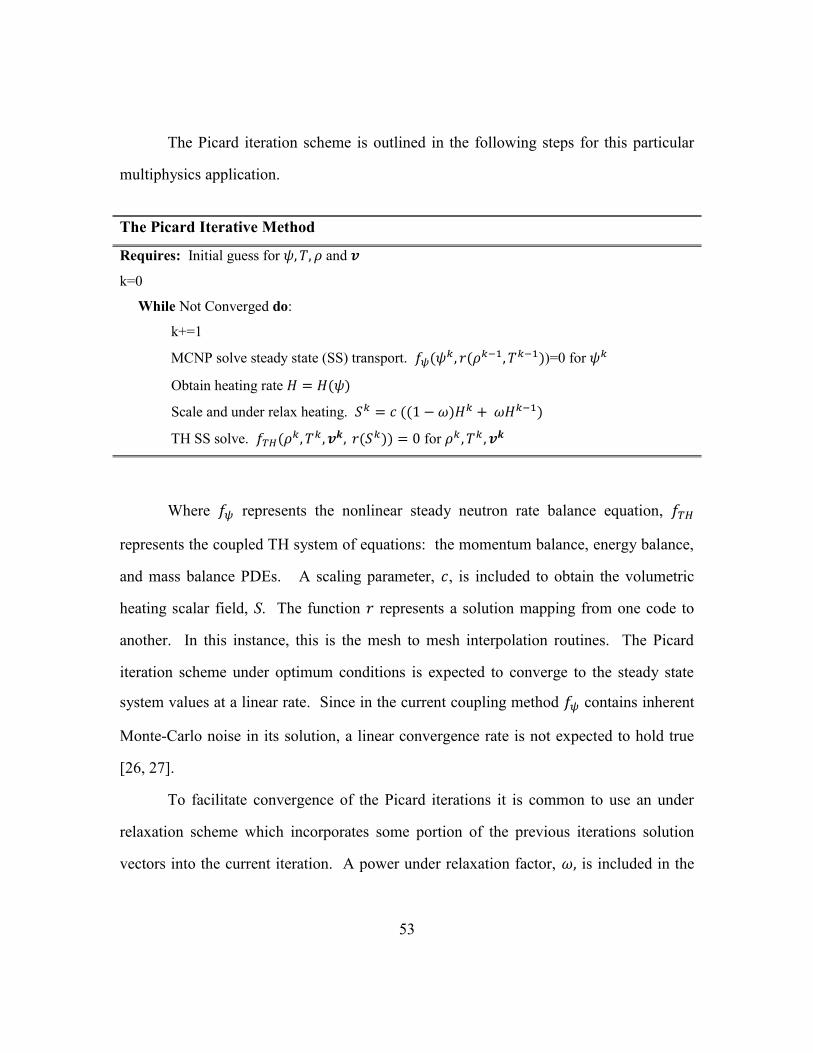
The Picard iteration scheme is outlined in the following steps for this particular
multiphysics application.
The Picard Iterative Method
Requires: Initial guess for 𝜓, 𝑇, 𝜌 and 𝒗
k=0
While Not Converged do:
k+=1
MCNP solve steady state (SS) transport. 𝑓𝜓(𝜓𝑘, 𝑟(𝜌𝑘−1, 𝑇𝑘−1))=0 for 𝜓𝑘
Obtain heating rate 𝐻 = 𝐻(𝜓)
Scale and under relax heating. 𝑆𝑘 = 𝑐 ((1 − 𝜔)𝐻𝑘 + 𝜔𝐻𝑘−1)
TH SS solve. 𝑓𝑇𝐻(𝜌𝑘, 𝑇𝑘 , 𝒗𝒌, 𝑟(𝑆𝑘)) = 0 for 𝜌𝑘 , 𝑇𝑘 , 𝒗𝒌
Where 𝑓𝜓 represents the nonlinear steady neutron rate balance equation, 𝑓𝑇𝐻
represents the coupled TH system of equations: the momentum balance, energy balance,
and mass balance PDEs. A scaling parameter, 𝑐, is included to obtain the volumetric
heating scalar field, S. The function 𝑟 represents a solution mapping from one code to
another. In this instance, this is the mesh to mesh interpolation routines. The Picard
iteration scheme under optimum conditions is expected to converge to the steady state
system values at a linear rate. Since in the current coupling method 𝑓𝜓 contains inherent
Monte-Carlo noise in its solution, a linear convergence rate is not expected to hold true
[26, 27].
To facilitate convergence of the Picard iterations it is common to use an under
relaxation scheme which incorporates some portion of the previous iterations solution
vectors into the current iteration. A power under relaxation factor, 𝜔, is included in the

54
Picard solution in the current application. This has the effect of damping oscillations in
the power profile that may be present between solution updates.
Two factors influence oscillations in the power profile between solution updates
in the current coupled system. The first is due to the repeated application of an
approximate Picard solution update procedure to system of coupled non-linear equations.
Oscillations are damped if the system has sufficient negative feedbacks, provided in the
cases investigated in this thesis by negative thermal reactivity coefficients or by
introducing artificial dampening by under relaxation. Secondly, small fluctuations due to
residual Monte Carlo noise persist in the heating tally result vector despite a slight
reduction in magnitude by under-relaxation. These small fluctuations can be defeated by
either running more particle histories in MCNP per Picard iteration or by averaging
together many past energy deposition solution vectors into the current iterate by a
weighted averaging process.
It is of interest to consider fixed point numerical methods with improved
convergence characteristics over the basic Picard iteration scheme. Principle among
them are Newton based iterations in which an approximate Jacobian computation must be
performed. If the Jacobian is computationally costly or prohibitively difficult to estimate,
motivation remains to use Jacobian free methods. To this end, the application of
Anderson acceleration to fixed point problems that arise in core simulation calculations is
an active field of research [28]. In some circumstances Anderson acceleration may be
viewed as a direct upgrade to the Picard iteration scheme. Few modifications to the
Picard algorithm, and thus the implementation in code, are required to adopt its use in
multiphysics applications. Shown in equation 13, Anderson acceleration attempts to find
a linear combination of the previous M solution vector differences, 𝐹𝑘.

55
𝐹𝑘 = 𝐺(𝑥𝑘) − 𝑥𝑘 (13)
that minimize the L2 norm:
{𝛼(𝑘)} = min𝛼
‖∑ 𝛼𝑖𝐹𝑘−𝑀+𝑖
𝑀
𝑖=0
‖ (14)
With the constraint:
∑ 𝛼𝑖 = 1
𝑖=0
Where 𝑘 is the current iteration number and 𝑀 = min ({𝑘, 𝑚}) where 𝑚 is a user set max
solution vector storage depth. In an Anderson scheme with no additional under
relaxation (sometimes referred to as mixing), the solution is updated by equation 15:
𝑥𝑘+1 = ∑ 𝛼𝑖(𝑘)
𝐺(𝑥𝑘−𝑀+𝑖)
𝑀
𝑖
(15)
This is akin to the minimal residual method for solving coupled linear equations
known as GMRES. It can be shown that Anderson acceleration does not perform as
intended if significant noise in the solution is introduced by the mapping of the old
solution vector to the new, such in the case of using Monte Carlo methods [27]. Noise in
the solution update affects the ability to meaningfully and accurately solve the Anderson
minimization problem. Despite not being able to employ Anderson acceleration directly
in the current work, it provides a good starting point for the implementation of an
improved under-relaxation strategy in future Monte Carlo – CFD style couplings.

56
CHAPTER 4
Results
In this chapter MCNP-FLUENT is applied to suite of progressively more
challenging geometries and operating conditions to demonstrate the accuracy and
scalability of the coupling method. First, a unit fuel cell at hot zero power conditions is
studied to quantify error induced in the neutron multiplication factor by using a first-
order finite element representation of the geometry in MCNP rather than the traditional,
exact constructive solid geometry (CSG) representation. Following the zero power case,
a 2D plane wall geometry three meters in height with a moderator to fuel ratio of 1:1 is
studied at full power conditions. A degree of geometric complexity is added by
simulating a single PWR fuel pin at full and 75% nominal power conditions. Finally, a
3x3 fuel pin assembly without spacer grids is modeled and the coupled solution is
contrasted against results provided by the MPCAT-CTF package available in VERA.
The collective suite of results provides data necessary to assess the scalability of
the multiphysics coupling method. Run time versus number of cells present in the
MCNP and FLUENT simulations is charted in section 4.5.
4.1 2D UNIT CELL HOT ZERO POWER
The purpose of this case is to study the reactivity worth of using MCNP’s
unstructured mesh capability to represent PWR fuel geometries with respect to the
constructive solid geometry representation of the same geometry. In addition, run time as
a function of number of elements included in the mesh is recorded.
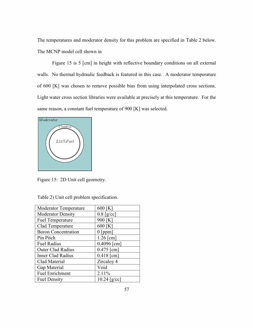
57
The temperatures and moderator density for this problem are specified in Table 2 below.
The MCNP model cell shown in
Figure 15 is 5 [cm] in height with reflective boundary conditions on all external
walls. No thermal hydraulic feedback is featured in this case. A moderator temperature
of 600 [K] was chosen to remove possible bias from using interpolated cross sections.
Light water cross section libraries were available at precisely at this temperature. For the
same reason, a constant fuel temperature of 900 [K] was selected.
Figure 15: 2D Unit cell geometry.
Table 2) Unit cell problem specification.
Moderator Temperature 600 [K]
Moderator Density 0.8 [g/cc]
Fuel Temperature 900 [K]
Clad Temperature 600 [K]
Boron Concentration 0 [ppm]
Pin Pitch 1.26 [cm]
Fuel Radius 0.4096 [cm]
Outer Clad Radius 0.475 [cm]
Inner Clad Radius 0.418 [cm]
Clad Material Zircaloy 4
Gap Material Void
Fuel Enrichment 2.11%
Fuel Density 10.24 [g/cc]

58
Figure 16: Left: Top view of a pin cell finite element geometry displayed in quarter
symmetry. 6 azimuthal segregations per quartile are shown. The
discrepancy between the FE mesh and the CSG geometry is shown on the
right.
The pin dimensions, given in Table 2 are consistent with typical Westinghouse PWR fuel
design [29]. Shown in Figure 16 an approximation of the true geometry by first order
cells gives rise to differences in both the fuel and moderator volume. This geometry
discrepancy impacts neutron moderation near the cladding moderator boundary and the
amount of fissile material in the problem. A reactivity difference of 52 [pcm] relative to
the CSG base case is seen using sixteen azimuthal fuel segments per quadrant.
Eigenvalue results for the unit cell case are presented in Table 3.
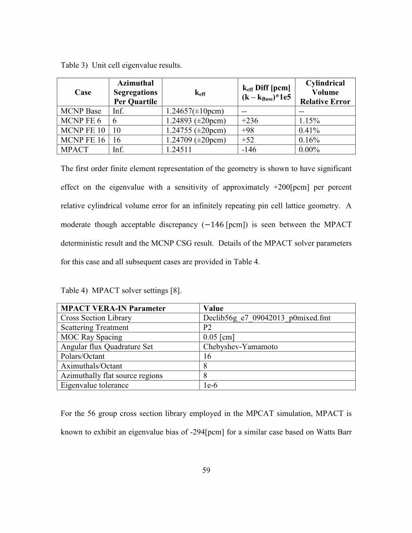
59
Table 3) Unit cell eigenvalue results.
Case
Azimuthal
Segregations
Per Quartile
keff keff Diff [pcm]
(k – kBase)*1e5
Cylindrical
Volume
Relative Error
MCNP Base Inf. 1.24657(±10pcm) -- --
MCNP FE 6 6 1.24893 (±20pcm) +236 1.15%
MCNP FE 10 10 1.24755 (±20pcm) +98 0.41%
MCNP FE 16 16 1.24709 (±20pcm) +52 0.16%
MPACT Inf. 1.24511 -146 0.00%
The first order finite element representation of the geometry is shown to have significant
effect on the eigenvalue with a sensitivity of approximately +200[pcm] per percent
relative cylindrical volume error for an infinitely repeating pin cell lattice geometry. A
moderate though acceptable discrepancy (−146 [pcm]) is seen between the MPACT
deterministic result and the MCNP CSG result. Details of the MPACT solver parameters
for this case and all subsequent cases are provided in Table 4.
Table 4) MPACT solver settings [8].
MPACT VERA-IN Parameter Value
Cross Section Library Declib56g_e7_09042013_p0mixed.fmt
Scattering Treatment P2
MOC Ray Spacing 0.05 [cm]
Angular flux Quadrature Set Chebyshev-Yamamoto
Polars/Octant 16
Aximuthals/Octant 8
Azimuthally flat source regions 8
Eigenvalue tolerance 1e-6
For the 56 group cross section library employed in the MPCAT simulation, MPACT is
known to exhibit an eigenvalue bias of -294[pcm] for a similar case based on Watts Barr
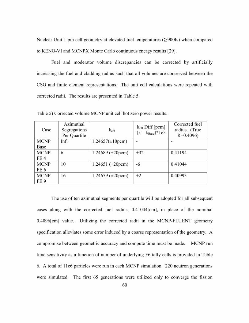
60
Nuclear Unit 1 pin cell geometry at elevated fuel temperatures (≥900K) when compared
to KENO-VI and MCNPX Monte Carlo continuous energy results [29].
Fuel and moderator volume discrepancies can be corrected by artificially
increasing the fuel and cladding radius such that all volumes are conserved between the
CSG and finite element representations. The unit cell calculations were repeated with
corrected radii. The results are presented in Table 5.
Table 5) Corrected volume MCNP unit cell hot zero power results.
Case
Azimuthal
Segregations
Per Quartile
keff keff Diff [pcm]
(k – kBase)*1e5
Corrected fuel
radius. (True
R=0.4096)
MCNP
Base
Inf. 1.24657(±10pcm) - -
MCNP
FE 4
6 1.24689 (±20pcm) +32 0.41194
MCNP
FE 6
10 1.24651 (±20pcm) -6 0.41044
MCNP
FE 9
16 1.24659 (±20pcm) +2 0.40993
The use of ten azimuthal segments per quartile will be adopted for all subsequent
cases along with the corrected fuel radius, 0.41044[cm], in place of the nominal
0.4096[cm] value. Utilizing the corrected radii in the MCNP-FLUENT geometry
specification alleviates some error induced by a coarse representation of the geometry. A
compromise between geometric accuracy and compute time must be made. MCNP run
time sensitivity as a function of number of underlying F6 tally cells is provided in Table
6. A total of 11e6 particles were run in each MCNP simulation. 220 neutron generations
were simulated. The first 65 generations were utilized only to converge the fission
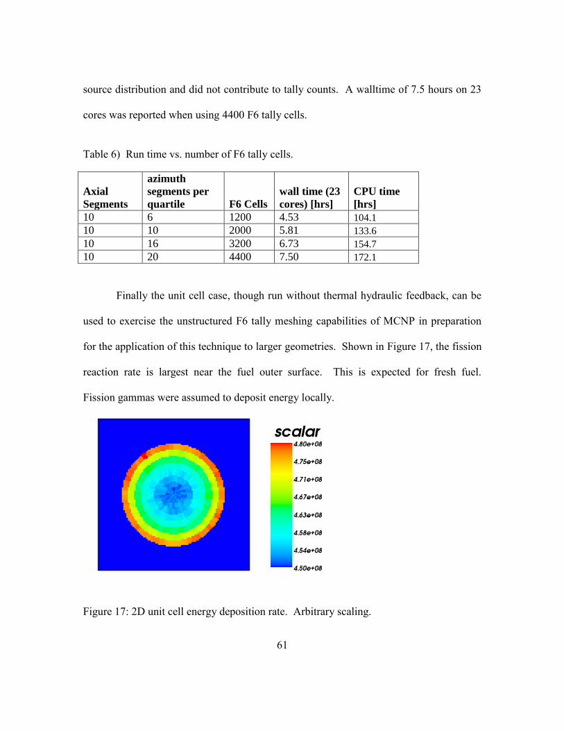
61
source distribution and did not contribute to tally counts. A walltime of 7.5 hours on 23
cores was reported when using 4400 F6 tally cells.
Table 6) Run time vs. number of F6 tally cells.
Axial
Segments
azimuth
segments per
quartile F6 Cells
wall time (23
cores) [hrs]
CPU time
[hrs]
10 6 1200 4.53 104.1
10 10 2000 5.81 133.6
10 16 3200 6.73 154.7
10 20 4400 7.50 172.1
Finally the unit cell case, though run without thermal hydraulic feedback, can be
used to exercise the unstructured F6 tally meshing capabilities of MCNP in preparation
for the application of this technique to larger geometries. Shown in Figure 17, the fission
reaction rate is largest near the fuel outer surface. This is expected for fresh fuel.
Fission gammas were assumed to deposit energy locally.
Figure 17: 2D unit cell energy deposition rate. Arbitrary scaling.
62
4.2 2D PLANE WALL
The purpose of this case is to exercise all components of the coupling
methodology using thermal hydraulic conditions and energy densities similar to a PWR
operating at low power while reducing the geometric complexity of the problem. A
convergence study was conducted for this case in which the number of MCNP particle
histories simulated per outer iteration was altered and the impact on convergence rate on
the power distribution was recorded. In addition section 4.2.5 investigates the sensitivity
of the coupled solution to the treatment of photon transport. Since this case consists of a
2D planar geometry, runtimes are kept to a minimum while the results of the sensitivity
studies remain relevant to the 3D full-height pin cell case.
This case also provides an opportunity to check for expected trends, such as
fission reaction rate depression in regions of low moderator density near the top of the
reactor geometry, effectively compressing the thermal energy production of the reactor
towards the bottom of the core slightly. The resolution of more detailed physics is also
demonstrated. A higher fission reaction rate is expected near the moderator-fuel
boundary where the thermal neutron population is largest in the fuel. A growing
boundary layer should be visible when studying velocity profiles as a function of axial
position in the moderator channel. Confidence in the software implementation of the
coupling methodology is built by successfully predicting expected trends with a
straightforward 2D case.
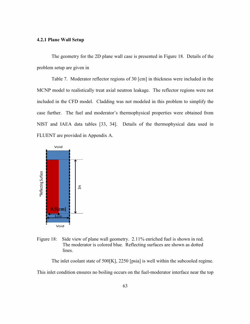
63
4.2.1 Plane Wall Setup
The geometry for the 2D plane wall case is presented in Figure 18. Details of the
problem setup are given in
Table 7. Moderator reflector regions of 30 [cm] in thickness were included in the
MCNP model to realistically treat axial neutron leakage. The reflector regions were not
included in the CFD model. Cladding was not modeled in this problem to simplify the
case further. The fuel and moderator’s thermophysical properties were obtained from
NIST and IAEA data tables [33, 34]. Details of the thermophysical data used in
FLUENT are provided in Appendix A.
Figure 18: Side view of plane wall geometry. 2.11% enriched fuel is shown in red.
The moderator is colored blue. Reflecting surfaces are shown as dotted
lines.
The inlet coolant state of 500[K], 2250 [psia] is well within the subcooled regime.
This inlet condition ensures no boiling occurs on the fuel-moderator interface near the top
0.5[cm]
64
of the coolant channel where temperatures are greatest. Ensuring boiling does not occur
simplifies the CFD calculation and problem setup by negating the need for a subcooled
boiling model.
Table 7) Plane wall problem setup.
Moderator Inlet Temperature 500 [K]
Pressure 2250 [psia]
Moderator Inlet Mass Flux 1200 [kg/m2s]
Moderator Reflector height 30 [cm]
Boron Concentration 0 [ppm]
Fuel and Moderator Half-Width 0.5 [cm]
Fuel Enrichment 2.11%
Fuel Density 10.24 [g/cc]
Active Fuel Height 3 [m]
Average Volumetric Heating (Power density) 6.0e7 [W/m3]
The parameters used in the FLUENT thermal hydraulic model are provided in Table 8. A
value of 3.4% turbulence intensity was used at the inlet as determined the empirical
relation for turbulence intensity for internal flows shown in equation 16 [20].
𝐼 = 0.16(𝑅𝑒)−1/8 (16)
With the Reynolds number given by:
𝑅𝑒 =𝜌𝑣𝐷𝑒
𝜇 (17)
And 𝐷𝑒 is the hydraulic diameter, given by equation 18:
𝐷𝑒 =4 𝐴𝑒
𝑊𝑝 (18)
Where 𝐴𝑒 is the area of the channel and 𝑊𝑝 is the wetted perimeter.
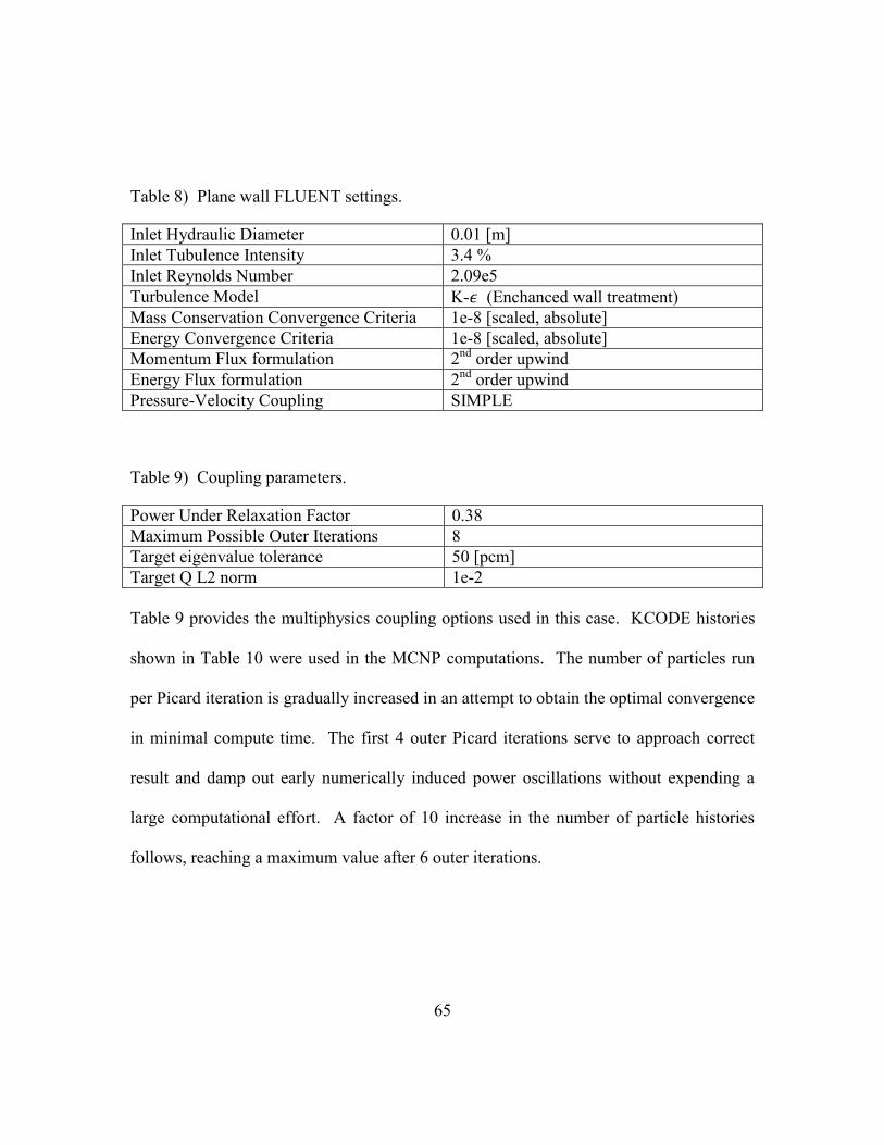
65
Table 8) Plane wall FLUENT settings.
Inlet Hydraulic Diameter 0.01 [m]
Inlet Tubulence Intensity 3.4 %
Inlet Reynolds Number 2.09e5
Turbulence Model K-𝜖 (Enchanced wall treatment)
Mass Conservation Convergence Criteria 1e-8 [scaled, absolute]
Energy Convergence Criteria 1e-8 [scaled, absolute]
Momentum Flux formulation 2nd
order upwind
Energy Flux formulation 2nd
order upwind
Pressure-Velocity Coupling SIMPLE
Table 9) Coupling parameters.
Power Under Relaxation Factor 0.38
Maximum Possible Outer Iterations 8
Target eigenvalue tolerance 50 [pcm]
Target Q L2 norm 1e-2
Table 9 provides the multiphysics coupling options used in this case. KCODE histories
shown in Table 10 were used in the MCNP computations. The number of particles run
per Picard iteration is gradually increased in an attempt to obtain the optimal convergence
in minimal compute time. The first 4 outer Picard iterations serve to approach correct
result and damp out early numerically induced power oscillations without expending a
large computational effort. A factor of 10 increase in the number of particle histories
follows, reaching a maximum value after 6 outer iterations.

66
Table 10) KCODE history for the plane wall case.
Outer Iteration Particles per
Generation
Inactive
Generations
Total Generations
1 2e4 200 400
2 2e4 ↓ 800
3 3e4 ↓ 800
4 4e4 ↓ 800
5 5e5 ↓ 800
6 ↓ ↓ 1200
7 ↓ ↓ 1200
8 ↓ ↓ 1200
A summary of the MCNP and FLUENT mesh statistics is given in Table 11. As
discussed in section 3.1.1, the MCNP geometry is coarsely subdivided into bodies inside
which unique temperatures and densities are tracked. The fuel region was subdivided
into 12 axial 2 equal-sized radial regions; the moderator channel was segregated into 12
axial regions.
Table 11) MCNP and FLUENT mesh statistics for the 2D plane wall case.
Discritization Number of Elements
Total MCNP UM parts 34
Total MCNP F6 tally cells 488
Total FLUENT cells 43452
4.2.2 2D Plane Wall Results
Eigenvalue results and convergence history of the normalized power distribution
are given in Table 12. The target eigenvalue tolerance of 50 [pcm] was easily met. The
target L2 Qnorm tolerance of 1e-2 was nearly obtained, but small fluctuations in the
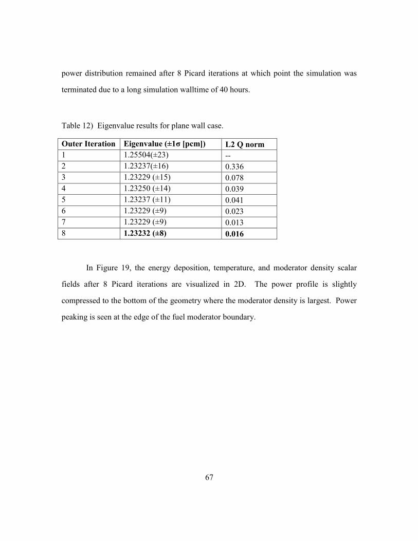
67
power distribution remained after 8 Picard iterations at which point the simulation was
terminated due to a long simulation walltime of 40 hours.
Table 12) Eigenvalue results for plane wall case.
Outer Iteration Eigenvalue (±1σ [pcm]) L2 Q norm
1 1.25504(±23) --
2 1.23237(±16) 0.336
3 1.23229 (±15) 0.078
4 1.23250 (±14) 0.039
5 1.23237 (±11) 0.041
6 1.23229 (±9) 0.023
7 1.23229 (±9) 0.013
8 1.23232 (±8) 0.016
In Figure 19, the energy deposition, temperature, and moderator density scalar
fields after 8 Picard iterations are visualized in 2D. The power profile is slightly
compressed to the bottom of the geometry where the moderator density is largest. Power
peaking is seen at the edge of the fuel moderator boundary.

68
Figure 19: Left: Energy Deposition [W/m3]. Center: Temperature [K]. Right:
Moderator density [g/cc]. Geometry not to scale.
The velocity field within the moderator channel may be extracted from the CFD results
and plotted as velocity profiles as function of axial position. Given a Reynolds number of
~2e5, well within the turbulent regime, the entrance length is estimated to be 0.34 [m] by
the empirical relationship shown in equation 19 [30].
𝐿𝑒 = 𝐷𝑒(4.4𝑅𝑒16)
(19)
Plots of the moderator velocity profiles are shown in Figure 20. Only very small changes
in the profile shape are seen past 0.5 [m] indicating a fully developed flow has been
achieved. In accordance with mass conservation, the average velocity magnitude across
the channel increases slightly as the coolant density falls as it travels up the channel.
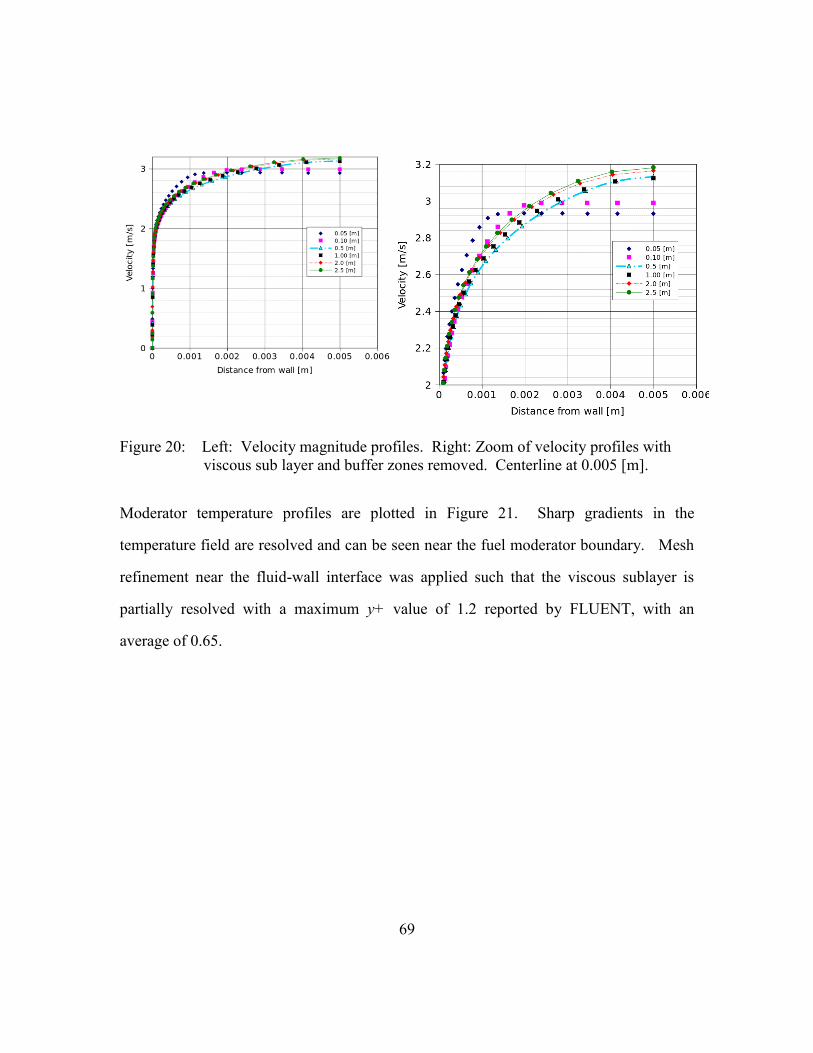
69
Figure 20: Left: Velocity magnitude profiles. Right: Zoom of velocity profiles with
viscous sub layer and buffer zones removed. Centerline at 0.005 [m].
Moderator temperature profiles are plotted in Figure 21. Sharp gradients in the
temperature field are resolved and can be seen near the fuel moderator boundary. Mesh
refinement near the fluid-wall interface was applied such that the viscous sublayer is
partially resolved with a maximum y+ value of 1.2 reported by FLUENT, with an
average of 0.65.

70
Figure 21: Plane wall moderator temperature profiles.
Figure 22: Fuel-Moderator interface axial temperature profile.
A plot of the moderate/fuel interface temperature is given in Figure 22. A maximum
moderator temperature of 543[K] is achieved near the axial position of 1.8 [m] at the fuel
moderator interface. From this plot it can be seen that energy deposition tally
information passed from MCNP to FLUENT is coarsely resolved in the axial direction in
relation to the CFD mesh. FLUENT’s built in scalar field import functionality maps the

71
incoming data to the CFD mesh utilizing a piecewise constant formulation. In addition,
axial thermal energy diffusion within the fuel is minimal due to the radialy thin geometry
and small thermal conductivity of the Uranium oxide fuel. Therefore small steps are
visible in the axial interface temperature plot.
Figure 23: Plane wall FLUENT convergence behavior. Five outer iterations shown.
Figure 23 displays mass, energy, momentum and turbulence TH balance residuals
for five consecutive outer iterations. The convergence rate of the SIMPLE iterative
method is rapid in this case: The energy and mass conservation equations were satisfied
within the specified tolerance of 1e-8 in approximately 320 SIMPLE iterations per outer
iteration. Outer iterations are visibly delimited in the residual plot as sharp increases in
the scaled residuals when the energy deposition scalar field is updated.

72
Figure 24: Normalized energy deposition rate inside the fuel region.
Figure 25: Left: Volume averaged fuel temperature. Right: Volume averaged
moderator temperature in the coolant channel as a function of distance to the
bottom of the active fuel.
Radially averaged power density and temperature results are provided in figures
Figure 24 andFigure 25 respectively. The power density plot depicts convergence
behavior by plotting multiple Picard iterations with the final solution provided as a bold
black line. These quantities are conveniently compared to results from other reactor
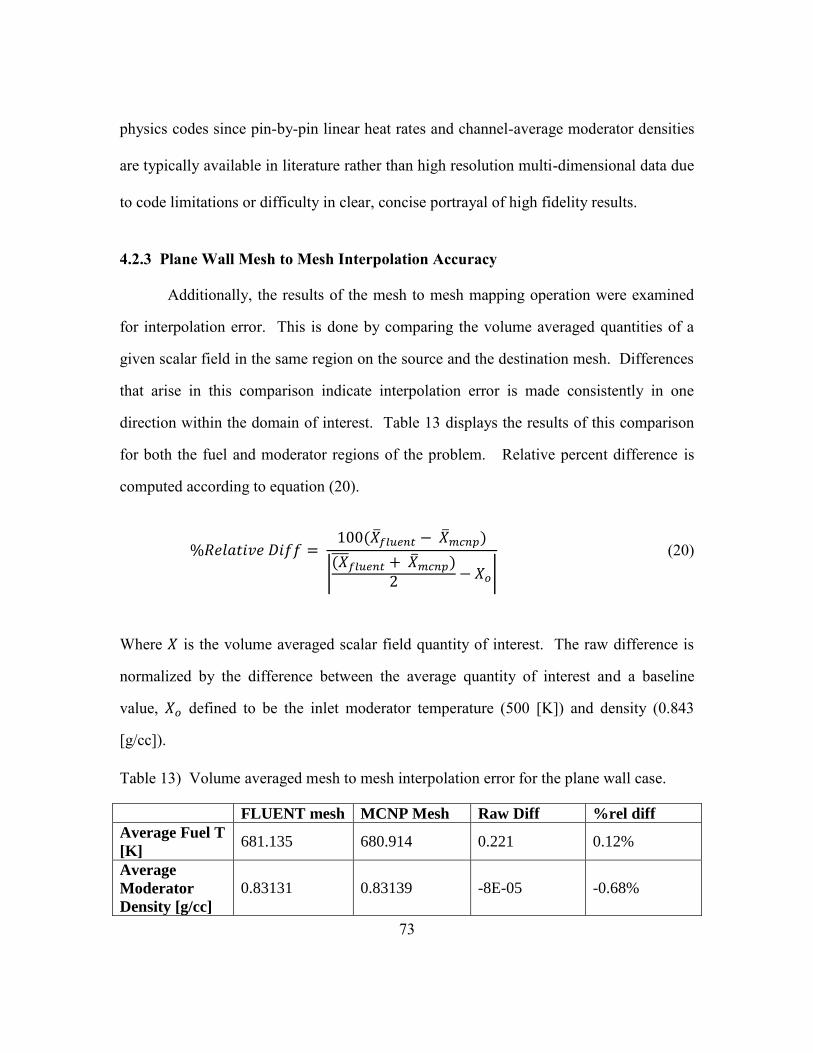
73
physics codes since pin-by-pin linear heat rates and channel-average moderator densities
are typically available in literature rather than high resolution multi-dimensional data due
to code limitations or difficulty in clear, concise portrayal of high fidelity results.
4.2.3 Plane Wall Mesh to Mesh Interpolation Accuracy
Additionally, the results of the mesh to mesh mapping operation were examined
for interpolation error. This is done by comparing the volume averaged quantities of a
given scalar field in the same region on the source and the destination mesh. Differences
that arise in this comparison indicate interpolation error is made consistently in one
direction within the domain of interest. Table 13 displays the results of this comparison
for both the fuel and moderator regions of the problem. Relative percent difference is
computed according to equation (20).
%𝑅𝑒𝑙𝑎𝑡𝑖𝑣𝑒 𝐷𝑖𝑓𝑓 = 100(��𝑓𝑙𝑢𝑒𝑛𝑡 − ��𝑚𝑐𝑛𝑝)
|(𝑋
𝑓𝑙𝑢𝑒𝑛𝑡 + ��𝑚𝑐𝑛𝑝)2 − 𝑋𝑜|
(20)
Where 𝑋 is the volume averaged scalar field quantity of interest. The raw difference is
normalized by the difference between the average quantity of interest and a baseline
value, 𝑋𝑜 defined to be the inlet moderator temperature (500 [K]) and density (0.843
[g/cc]).
Table 13) Volume averaged mesh to mesh interpolation error for the plane wall case.
FLUENT mesh MCNP Mesh Raw Diff %rel diff
Average Fuel T
[K] 681.135 680.914 0.221 0.12%
Average
Moderator
Density [g/cc]
0.83131 0.83139 -8E-05 -0.68%

74
For the plane wall case in which the MCNP and FLUENT meshes are nearly
identical due to the geometric simplicity of the problem, only small interpolation error is
seen. Interpolation error arises due to non-conformal cells (i.e. cell overlap). Bias in the
mapping is introduced if interpolation errors are consistently made in the same direction
over the domain. Since the mesh to mesh mapping routine employed in this thesis is not
conservative, minor errors are introduced in mapping between two different meshes.
Conservative mesh to mesh transfer conserves integral quantities in the solution mapping
process. See Data Transfer Kit’s documentation for information on conservative mesh to
mesh solution transfers [30].
4.2.4 Plane Wall Convergence Rate Study
Two sources of error from the neutronics calculation contribute to coupled
solution defects. Non fundamental mode harmonics may persist in the spatial neutron
flux distribution as a consequence of the iterative technique used by MCNP to solve the
k-eigenvalue problem. See section 2.2.1 for details of the iterative procedure used to
solve the k-eigenvalue problem. This source of error is reduced by running a larger
number of simulated neutron generations, effectively allowing higher harmonics to decay
away. Secondly, Monte Carlo noise is present in the heating tally. Monte Carlo noise in
the heating tally can be reduced by either by computing integrals quantities over larger
volumes, or by running a larger number of particle histories. Given limited
computational resources, a balance between grid fidelity and total number of particle
histories should be struck such that the coupled solution is independent of grid spacing.
Obtaining the ideal mesh density and number of particle histories run per outer Picard
iteration is left as an avenue for future work. The presented results only serve to quantify
the benefits of running a larger number of particle histories.
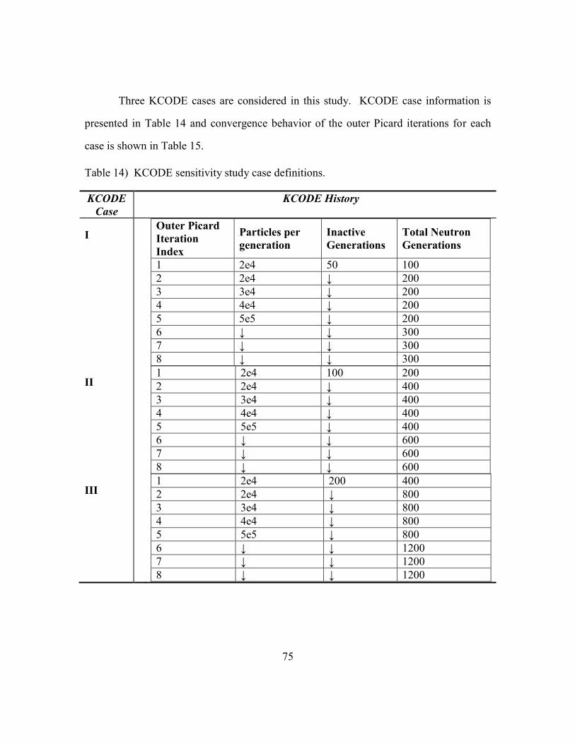
75
Three KCODE cases are considered in this study. KCODE case information is
presented in Table 14 and convergence behavior of the outer Picard iterations for each
case is shown in Table 15.
Table 14) KCODE sensitivity study case definitions.
KCODE
Case
KCODE History
I Outer Picard
Iteration
Index
Particles per
generation
Inactive
Generations
Total Neutron
Generations
1 2e4 50 100
2 2e4 ↓ 200
3 3e4 ↓ 200
4 4e4 ↓ 200
5 5e5 ↓ 200
6 ↓ ↓ 300
7 ↓ ↓ 300
8 ↓ ↓ 300
II 1 2e4 100 200
2 2e4 ↓ 400
3 3e4 ↓ 400
4 4e4 ↓ 400
5 5e5 ↓ 400
6 ↓ ↓ 600
7 ↓ ↓ 600
8 ↓ ↓ 600
III 1 2e4 200 400
2 2e4 ↓ 800
3 3e4 ↓ 800
4 4e4 ↓ 800
5 5e5 ↓ 800
6 ↓ ↓ 1200
7 ↓ ↓ 1200
8 ↓ ↓ 1200

76
The maximum relative local power (Q) difference between Picard iterations
provides an estimate of the variability is present in the power distribution and is given by
equation 21. The L2 power norm is the root mean squared (RMS) of the power profile
differences between outer iterations and is computed by equation 22.
𝑚𝑎𝑥 Δ𝑄𝑖 = max [|𝑃𝑗
𝑖 − 𝑃𝑗𝑖−1|
𝑃𝑗𝑖
] (21)
𝐿2 𝑄 𝑛𝑜𝑟𝑚𝑖 = √∑ (𝑃𝑗
𝑖 − 𝑃𝑗𝑖−1
𝑃𝑗𝑖
)
2
𝑗
(22)
Where 𝑖 is the iteration number, 𝑗 is the axial position index and P is the normalized
linear heat rate. The power normalization is performed such that for the full core, the
axial linear power [W/m] profile averages to one.
Case I exhibits good initial convergence rate, obtaining an order of magnitude
reduction in the L2 norm after 4 iterations were completed, but stagnates after 5
iterations. Further solution convergence is hampered by Monte Carlo noise present in the
heating tally result and numerical oscillations in the neutron fission source distribution.
A larger number of simulated particle histories per Picard iteration are required to further
reduce the L2 norm of the power distribution. Case II shows moderate improvement in
Picard convergence over case I; however local relative power oscillations of ±2.5%
remain after 8 outer iterations were performed. Case III, having the largest number of
particles simulated per outer iteration, achieves the tightest convergence as indicated by
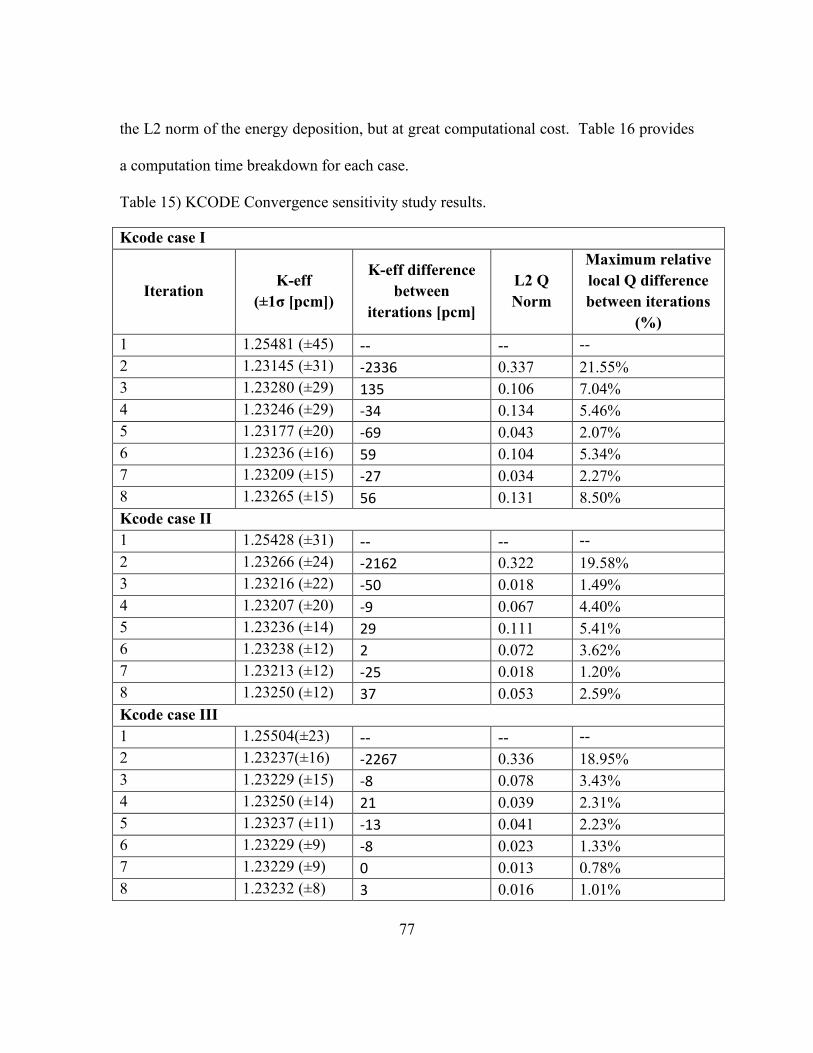
77
the L2 norm of the energy deposition, but at great computational cost. Table 16 provides
a computation time breakdown for each case.
Table 15) KCODE Convergence sensitivity study results.
Kcode case I
Iteration K-eff
(±1σ [pcm])
K-eff difference
between
iterations [pcm]
L2 Q
Norm
Maximum relative
local Q difference
between iterations
(%)
1 1.25481 (±45) -- -- --
2 1.23145 (±31) -2336 0.337 21.55%
3 1.23280 (±29) 135 0.106 7.04%
4 1.23246 (±29) -34 0.134 5.46%
5 1.23177 (±20) -69 0.043 2.07%
6 1.23236 (±16) 59 0.104 5.34%
7 1.23209 (±15) -27 0.034 2.27%
8 1.23265 (±15) 56 0.131 8.50%
Kcode case II
1 1.25428 (±31) -- -- --
2 1.23266 (±24) -2162 0.322 19.58%
3 1.23216 (±22) -50 0.018 1.49%
4 1.23207 (±20) -9 0.067 4.40%
5 1.23236 (±14) 29 0.111 5.41%
6 1.23238 (±12) 2 0.072 3.62%
7 1.23213 (±12) -25 0.018 1.20%
8 1.23250 (±12) 37 0.053 2.59%
Kcode case III
1 1.25504(±23) -- -- --
2 1.23237(±16) -2267 0.336 18.95%
3 1.23229 (±15) -8 0.078 3.43%
4 1.23250 (±14) 21 0.039 2.31%
5 1.23237 (±11) -13 0.041 2.23%
6 1.23229 (±9) -8 0.023 1.33%
7 1.23229 (±9) 0 0.013 0.78%
8 1.23232 (±8) 3 0.016 1.01%

78
Table 16) KCODE study compute time summary. Wall times summed over all outer
iterations. 23 Cores used for FLUENT and MCNP calculations.
KCODE CASE
Total MCNP
Wall Time
[hr]
Total
FLUENT
Wall Time
[hr]
Total
Overhead
Wall Time [hr]
Total [hr]
I 10.16 0.17 0.0021 10.34
II 20.19 0.17 0.0021 20.36
III 40.34 0.17 0.0021 40.51
Improving the Picard convergence rate and tolerance is a computationally
expensive endeavor for the MCNP-FLUENT coupling method. The majority of the
computational expenditure is made in the Monte Carlo calculation. As demonstrated by
the runtime results provided Table 6, significant runtime reduction can be made by
reducing the number of F6 heating tally cells in MCNP though caution should be
observed so that the predicted behavior of the coupled system is not influenced by grid
spacing. Averaging the final three L2 power norms for cases I, II, and III yields averaged
norms of 0.090, 0.048, and 0.017 respectively. For this particular geometric
configuration, a two fold increase in the total number of particles run results in a
reduction in the minimal achievable L2 power norm tolerance by a factor of
approximately ½. This benefit requires a two-fold increase in computation time.
4.2.5 Plane Wall Gamma Transport Sensitivity
Table 17 provides the fraction of energy produced by fission that was absorbed in
the moderator channel. A large fraction of the energy deposition in the moderator is due

79
to neutron collision heating while the remainder heating is due to gamma ray interactions
with the moderator. The ability to toggle photon transport and photon heating is trivial in
MCNP, requiring modification of the F6 tally card and the transport MODE card. A
0.19% increase in the energy deposited in the moderator channel was observed when
photon transport was enabled, an insignificant difference.
Table 17) Fraction of energy deposited in the moderator channel.
Gamma Transport
Average Energy
Deposition in fuel
[W]
Average Energy
Deposition in
moderator [W]
Percent energy
deposited in
moderator
Off 6813.8 245.679 3.48%
On 6806.7 259.145 3.67%
Figure 26: Comparison of the plane wall energy deposition with gamma transport
enabled and disabled in MCNP.
80
Figure 26 shows the predicted power distributions after 8 Picard iterations were
performed. The power distribution was not discernibly impacted by enabling gamma
transport. As discussed in section 4.2.4, a relative maximum percent difference of 2.2%
in the local normalized power is within the expected fluctuations in the solution due to
residual numerical oscillations in the solution. The KCODE cycle history for this study
was identical to Case II in section 4.2.4. In all remaining cases, gamma rays will not be
tracked in the MCNP simulations and assumed to deposit their energy locally when
generated by fission events.
4.2.6 Plane Wall Conclusions
The plane wall case provided a test-stand in which all aspects of the MCNP-
FLUENT coupling method could be exercised. The axial power profile was shown to be
cosine in shape with slight power bias towards the moderator inlet. Plots of the
moderator velocity field were provided to demonstrate the level of detail produced by the
CFD computations. These detailed velocity and pressure field data are required to tune
pressure loss and turbulent mixing coefficients used by lower fidelity nodal TH codes
such as CTF. Furthermore, a review of the scaled mass, energy and momentum balance
residuals provided by ANSYS FLUENT showed the excellent convergence rate of the
SIMPLE pressure-velocity coupling scheme, with only 150 iterations per outer
(FLUENT/MCNP) iteration required for this case.
Relatively small runtimes allowed an investigation of eigenvalue and power
profile convergence as a function of number of particle histories utilized in each MCNP
run. Evidence of improved convergence achieved by increasing the number of particle
81
histories run in MCNP as measured by the L2 norm of the power profile, maximum
relative change in the power profile, and change in the eigenvalue between outer
iterations was put forth in Table 15. It was concluded that a reduction in uncertainty in
the power profile (with TH feedback enabled) by a factor of two required a factor of two
increase in compute time.
In cases where the total number of particle histories per KCODE cycle
approached 0.6 billion power oscillations persisted with a maximum magnitude of
approximately 1%. The key observation is that power oscillations can be reduced but
cannot be eliminated by increasing the particle count alone.
Finally, the impact of explicit gamma transport on the axial power profile was
shown to alter the results to a degree that lies within the uncertainty inherent in the result
due to residual power oscillations. Gamma transport will not be considered in the
following cases.
4.3 FULL HEIGHT SINGLE ROD
The purpose of this case is to compare the power, fuel temperature, and moderator
temperature distributions computed by MCNP-FLUENT to a solution provided by
MPCACT-CTF. The MPACT-CTF solver parameters were set according to the values
stated previously in Table 4. This is the first and simplest instance in which a coupled
solution may be compared between the two codes. Despite the problem’s simplicity,
disparate details in the solution method, cross section data, and thermophysical material
properties between the two codes can explain some small differences in the predicted
solutions. The problem was run at both 100% and 75% of nominal PWR operating

82
power conditions. Thermophysical material properties used in the FLUENT CFD
simulations are provided in Appendix A.
4.3.1 Problem Setup
A top down view of the single quarter symmetric rod is shown in Figure 27. The
problem was run in quarter symmetry in MCNP and in FLUENT to reduce computation
time. Reflecting boundary conditions were applied on all radial surfaces.
Figure 27: Top view of MCNP single fuel rod geometry in quarter symmetry.
Constituent pseudo-cells differentiated by color.
The fuel is zoned into two equal volume radial regions. A single radial cladding region is
used. The moderator is zoned by octant. In the figure, material zones are designated by
color. Spacer grids were not included in the MCNP or FLUENT models. 30[cm] thick
axial moderator reflector regions directly above and below the active fuel region were
included into the MCNP model to properly treat neutron leakage. The reflector regions
were not modeled in FLUENT. The fuel was subdivided into 2 radial and 22 axial zones.
The moderator channel was subdivided into 2 octant zones and 22 axial zones. The
problem geometric parameters are given in Table 18.
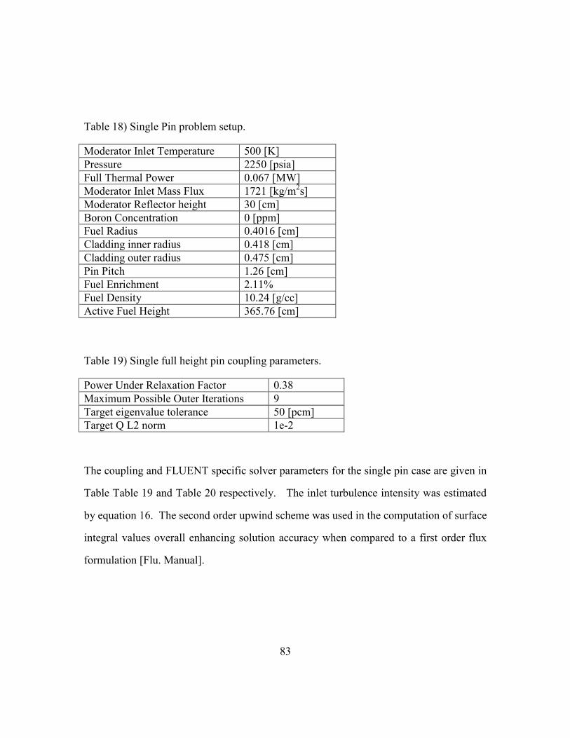
83
Table 18) Single Pin problem setup.
Moderator Inlet Temperature 500 [K]
Pressure 2250 [psia]
Full Thermal Power 0.067 [MW]
Moderator Inlet Mass Flux 1721 [kg/m2s]
Moderator Reflector height 30 [cm]
Boron Concentration 0 [ppm]
Fuel Radius 0.4016 [cm]
Cladding inner radius 0.418 [cm]
Cladding outer radius 0.475 [cm]
Pin Pitch 1.26 [cm]
Fuel Enrichment 2.11%
Fuel Density 10.24 [g/cc]
Active Fuel Height 365.76 [cm]
Table 19) Single full height pin coupling parameters.
Power Under Relaxation Factor 0.38
Maximum Possible Outer Iterations 9
Target eigenvalue tolerance 50 [pcm]
Target Q L2 norm 1e-2
The coupling and FLUENT specific solver parameters for the single pin case are given in
Table Table 19 and Table 20 respectively. The inlet turbulence intensity was estimated
by equation 16. The second order upwind scheme was used in the computation of surface
integral values overall enhancing solution accuracy when compared to a first order flux
formulation [Flu. Manual].
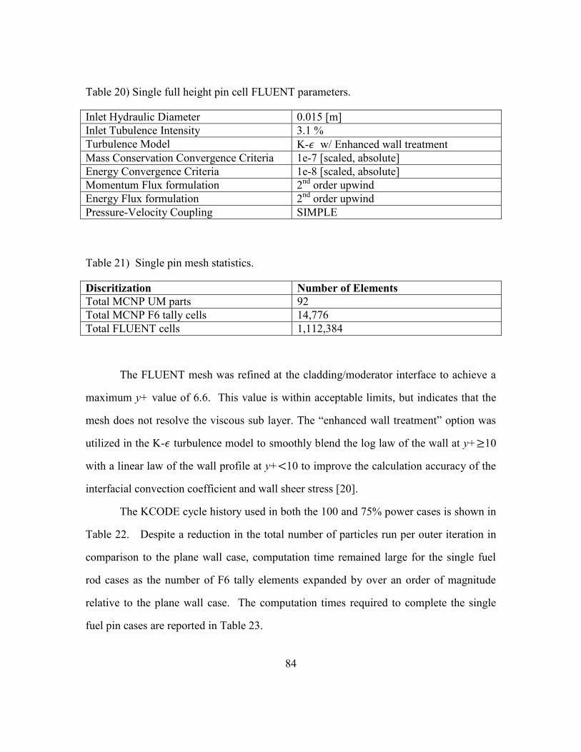
84
Table 20) Single full height pin cell FLUENT parameters.
Inlet Hydraulic Diameter 0.015 [m]
Inlet Tubulence Intensity 3.1 %
Turbulence Model K-𝜖 w/ Enhanced wall treatment
Mass Conservation Convergence Criteria 1e-7 [scaled, absolute]
Energy Convergence Criteria 1e-8 [scaled, absolute]
Momentum Flux formulation 2nd
order upwind
Energy Flux formulation 2nd
order upwind
Pressure-Velocity Coupling SIMPLE
Table 21) Single pin mesh statistics.
Discritization Number of Elements
Total MCNP UM parts 92
Total MCNP F6 tally cells 14,776
Total FLUENT cells 1,112,384
The FLUENT mesh was refined at the cladding/moderator interface to achieve a
maximum y+ value of 6.6. This value is within acceptable limits, but indicates that the
mesh does not resolve the viscous sub layer. The “enhanced wall treatment” option was
utilized in the K-𝜖 turbulence model to smoothly blend the log law of the wall at y+≥10
with a linear law of the wall profile at y+<10 to improve the calculation accuracy of the
interfacial convection coefficient and wall sheer stress [20].
The KCODE cycle history used in both the 100 and 75% power cases is shown in
Table 22. Despite a reduction in the total number of particles run per outer iteration in
comparison to the plane wall case, computation time remained large for the single fuel
rod cases as the number of F6 tally elements expanded by over an order of magnitude
relative to the plane wall case. The computation times required to complete the single
fuel pin cases are reported in Table 23.

85
Table 22) 1x1 KCODE history.
Outer Iteration Particles per
Generation
Inactive
Generations
Total Generations
1 3e4 100 400
2 3e4 200 800
3 3e4 200 800
4 3e4 300 1000
5 4e4 ↓ 1000
6 ↓ ↓ 1200
7 ↓ ↓ 1500
8 ↓ ↓ 1500
9 ↓ ↓ 1500
Table 23) 1x1 Full height pin cell computation time. Sum of all iterations.
Total MCNP
Wall Time (52
cores) [hr]
Total
FLUENT
Wall Time
(12 cores)
[hr]
Total
Overhead Wall
Time (1 core)
[hr]
Total [hr]
Total 73.60 0.87 0.051 74.52
4.3.2 1x1, 75% Power Results
The total energy produced by the fuel at 75% of the full power rating is 0.05025
[MW]. An outlet temperature of 534.26[K] is predicted by MCNP-FLUENT, a
difference of -0.4[K] compared to the MPACT-CTF result. Excellent agreement for the
moderator temperature along the length of the channel is seen in Figure 28. Since the
problem is run at steady state it is expected that the outlet moderator temperatures exhibit
excellent agreement in order to obey conservation of energy. Small differences in outlet
temperature are primarily due to differences in the thermophysical properties of water

86
between the FLUENT implementation (see Appendix A for details) and the steam tables
used in CTF [32, 33].
Figure 28: Coolant channel plots for the full height single pin case operating at 75%
power. Left: Moderator temperature profile. Right: Moderator density
profile.
Figure 29: MCNP-FLUENT vs. MPACT-CTF Power distribution comparison. Single
full height pin operating at 75% power conditions.
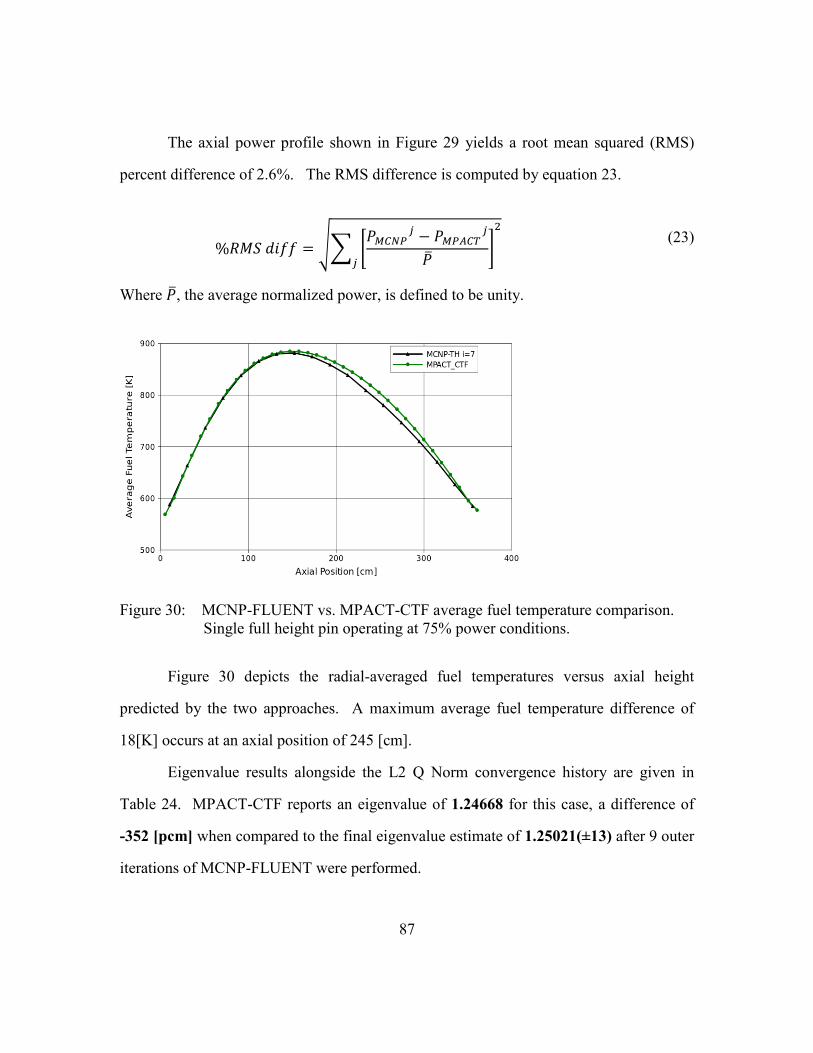
87
The axial power profile shown in Figure 29 yields a root mean squared (RMS)
percent difference of 2.6%. The RMS difference is computed by equation 23.
%𝑅𝑀𝑆 𝑑𝑖𝑓𝑓 = √∑ [𝑃𝑀𝐶𝑁𝑃
𝑗 − 𝑃𝑀𝑃𝐴𝐶𝑇𝑗
��]
2
𝑗
(23)
Where ��, the average normalized power, is defined to be unity.
Figure 30: MCNP-FLUENT vs. MPACT-CTF average fuel temperature comparison.
Single full height pin operating at 75% power conditions.
Figure 30 depicts the radial-averaged fuel temperatures versus axial height
predicted by the two approaches. A maximum average fuel temperature difference of
18[K] occurs at an axial position of 245 [cm].
Eigenvalue results alongside the L2 Q Norm convergence history are given in
Table 24. MPACT-CTF reports an eigenvalue of 1.24668 for this case, a difference of
-352 [pcm] when compared to the final eigenvalue estimate of 1.25021(±13) after 9 outer
iterations of MCNP-FLUENT were performed.
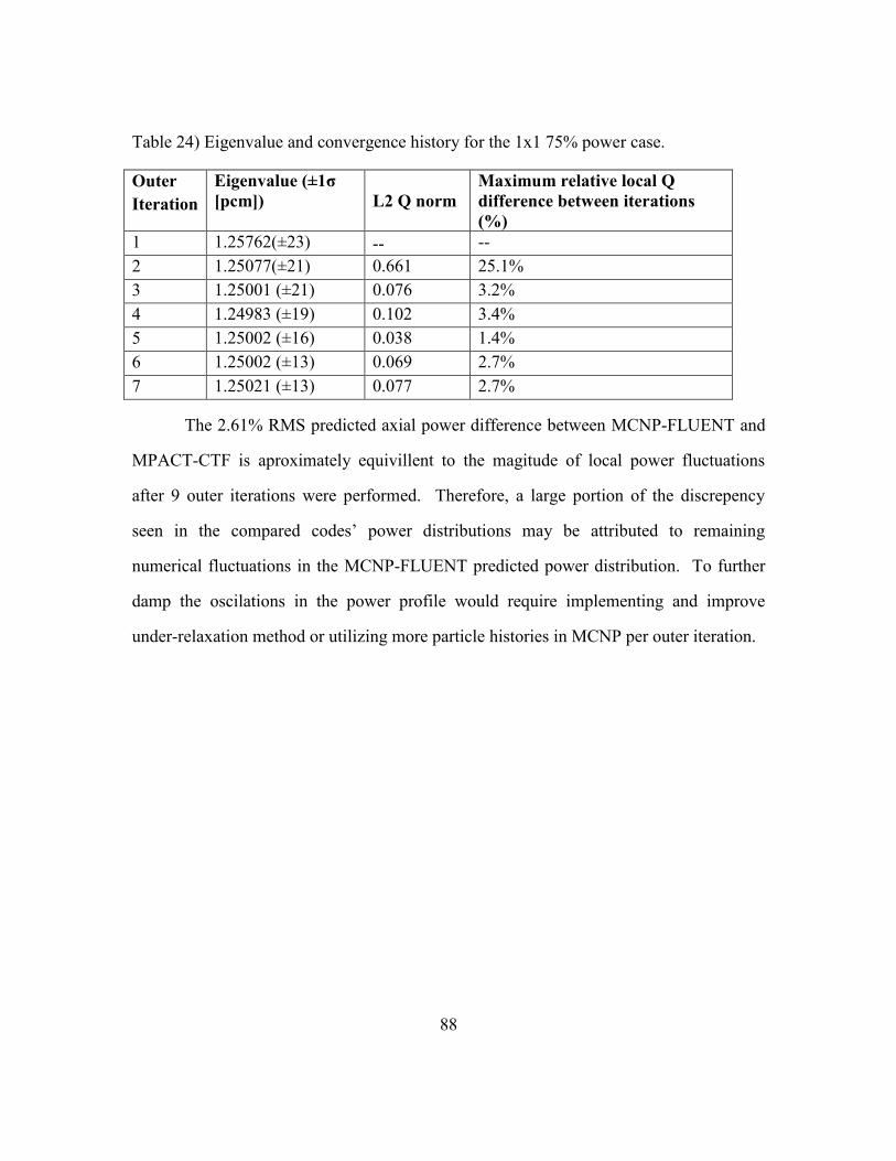
88
Table 24) Eigenvalue and convergence history for the 1x1 75% power case.
Outer
Iteration
Eigenvalue (±1σ
[pcm]) L2 Q norm
Maximum relative local Q
difference between iterations
(%)
1 1.25762(±23) -- --
2 1.25077(±21) 0.661 25.1%
3 1.25001 (±21) 0.076 3.2%
4 1.24983 (±19) 0.102 3.4%
5 1.25002 (±16) 0.038 1.4%
6 1.25002 (±13) 0.069 2.7%
7 1.25021 (±13) 0.077 2.7%
The 2.61% RMS predicted axial power difference between MCNP-FLUENT and
MPACT-CTF is aproximately equivillent to the magitude of local power fluctuations
after 9 outer iterations were performed. Therefore, a large portion of the discrepency
seen in the compared codes’ power distributions may be attributed to remaining
numerical fluctuations in the MCNP-FLUENT predicted power distribution. To further
damp the oscilations in the power profile would require implementing and improve
under-relaxation method or utilizing more particle histories in MCNP per outer iteration.
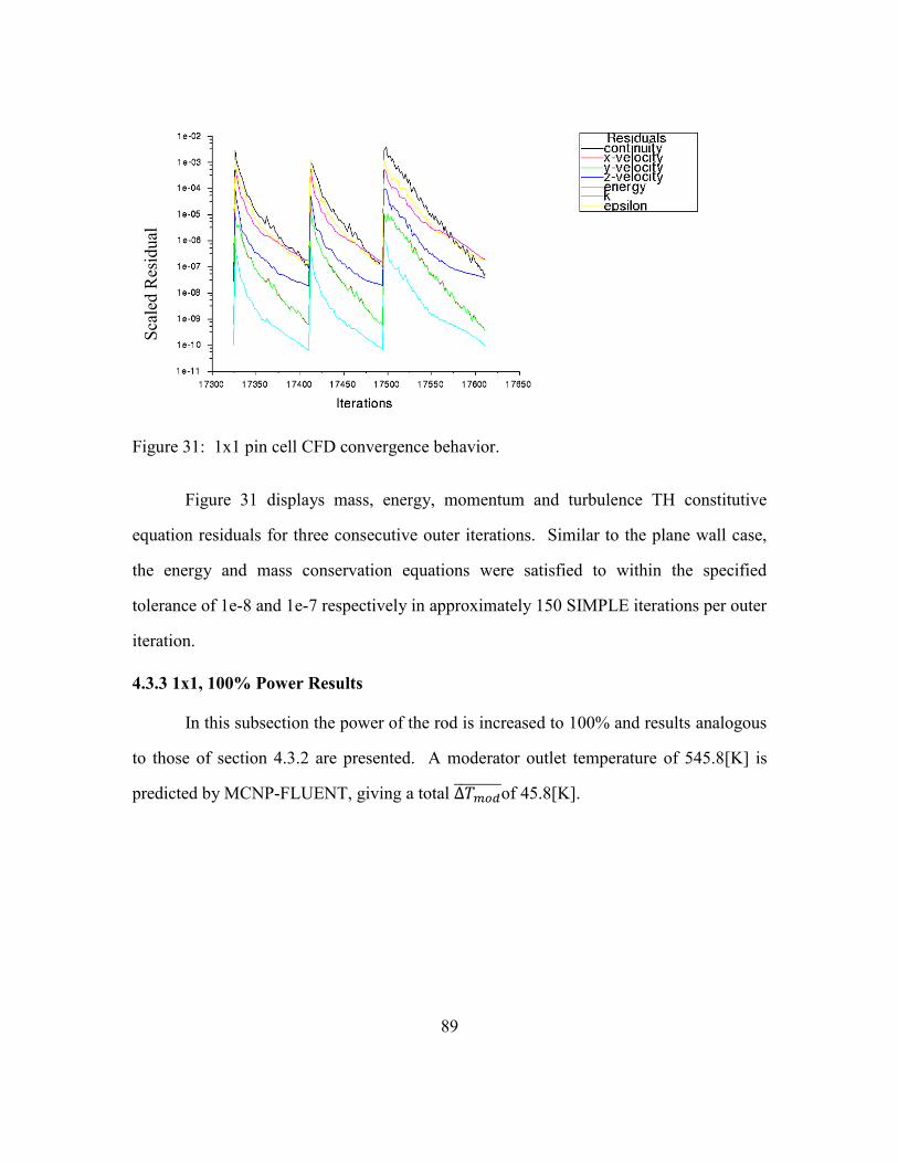
89
Figure 31: 1x1 pin cell CFD convergence behavior.
Figure 31 displays mass, energy, momentum and turbulence TH constitutive
equation residuals for three consecutive outer iterations. Similar to the plane wall case,
the energy and mass conservation equations were satisfied to within the specified
tolerance of 1e-8 and 1e-7 respectively in approximately 150 SIMPLE iterations per outer
iteration.
4.3.3 1x1, 100% Power Results
In this subsection the power of the rod is increased to 100% and results analogous
to those of section 4.3.2 are presented. A moderator outlet temperature of 545.8[K] is
predicted by MCNP-FLUENT, giving a total Δ𝑇𝑚𝑜𝑑 of 45.8[K].
Sca
led R
esid
ual

90
Figure 32: Coolant channel plots for the full height single pin case operating at 100%
power. Left: Moderator temperature profile. Right: Moderator density
profile.
In Figure 32 the MCNP-FLUENT moderator temperature and density traces
closely tracks the MPACT-CTF result. CTF yields an outlet temperature of 545.7[K]
giving and outlet temperature difference of 0.1[K].
Figure 33 displays differences in the predicted power profiles for this case. The
RMS axial power percent difference between MCNP-FLUENT and MPACT-CTF is
2.3%. The maximum relative difference is -4.0%.

91
Figure 33: MCNP-FLUENT vs. MPACT-CTF Power distribution comparison. Single
full height pin operating at 100% power conditions.
Seen in Figure 34, a maximum radially-averaged fuel temperature difference of
22[K] occurs at an axial location of 245[cm].
Figure 34: MCNP-FLUENT vs. MPACT-CTF average fuel temperature comparison.
Single full height pin operating at 100% power conditions.

92
Eigenvalue results and convergence history are provided in Table 25. MPACT-CTF
reports an eigenvalue of 1.24110 for this case, a difference of -355 [pcm] when compared
to the final MCNP-FLUENT eigenvalue result.
Table 25) Eigenvalue and convergence history for the 1x1 100% power case.
Outer
Iteration
Eigenvalue (±1σ
[pcm]) L2 Q
norm
Maximum relative local Q
difference between iterations (%)
1 1.25752 (±24) -- --
2 1.24578 (±21) 0.982 36.1%
3 1.24443 (±21) 0.140 6.2%
4 1.24487 (±18) 0.082 3.6%
5 1.24492 (±16) 0.132 5.1%
6 1.24446 (±13) 0.072 2.9%
7 1.24491 (±13) 0.062 2.7%
8 1.24468 (±12) 0.132 4.6%
9 1.24465 (±13) 0.118 3.8%
The maximum local power fluctuation in the MCNP-FLUENT coupled solution
after 9 outer iterations was approximately 3.8% in magnitude. Since a maximum power
differential of -4.0% between the compared codes was observed for this case, a large
portion of the discrepancy can be explained by numerical error due to undamped
oscillations remaining in the power profile.
4.3.4 1x1 Pin Cell Mesh to Mesh Interpolation Accuracy
Mesh to mesh interpolation error as measured by volume averaged scalar field
quantity comparisons between the MCNP and FLUENT meshes remains minimal for the
single pin case. The relative error reported in Table 26 is computed by equation (20).
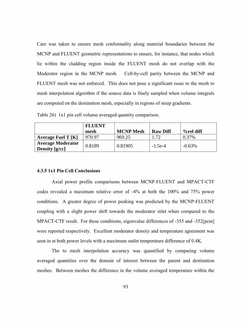
93
Care was taken to ensure mesh conformality along material boundaries between the
MCNP and FLUENT geometric representations to ensure, for instance, that nodes which
lie within the cladding region inside the FLUENT mesh do not overlap with the
Moderator region in the MCNP mesh. Cell-by-cell parity between the MCNP and
FLUENT mesh was not enforced. This does not pose a significant issue to the mesh to
mesh interpolation algorithm if the source data is finely sampled when volume integrals
are computed on the destination mesh, especially in regions of steep gradients.
Table 26) 1x1 pin cell volume averaged quantity comparison.
FLUENT
mesh MCNP Mesh Raw Diff %rel diff
Average Fuel T [K] 970.97 969.25 1.72 0.37%
Average Moderator
Density [g/cc] 0.8189 0.81905 -1.5e-4 -0.63%
4.3.5 1x1 Pin Cell Conclusions
Axial power profile comparisons between MCNP-FLUENT and MPACT-CTF
codes revealed a maximum relative error of -4% at both the 100% and 75% power
conditions. A greater degree of power peaking was predicted by the MCNP-FLUENT
coupling with a slight power shift towards the moderator inlet when compared to the
MPACT-CTF result. For these conditions, eigenvalue differences of -355 and -352[pcm]
were reported respectively. Excellent moderator density and temperature agreement was
seen in at both power levels with a maximum outlet temperature difference of 0.4K.
The to mesh interpolation accuracy was quantified by comparing volume
averaged quantities over the domain of interest between the parent and destination
meshes. Between meshes the difference in the volume averaged temperature within the

94
fuel-zone was shown to consistently remain less than 1%. Likewise, the volume
averaged moderator density between the two meshes was also less than 1%.
4.4 3X3 FUEL ROD ASSEMBLY
The 3x3 case represents a significant increase in geometric complexity compared
to the single pin, quarter symmetric case in the previous section. The 3x3 case affords
the opportunity to investigate the interplay of varied enrichments in each pin and empty
guide tubes on the axial and radial power distributions. In contrast to previous cases,
coolant cross flow plays an important role in the fluid model. Cross flow impacts the
moderator density and temperature fields which in turn affects the fuel reactivity.
Spacer grids were not included in the MCNP or FLUENT models. As in the previous
single pin case, the results of the MCNP-FLUENT calculations are compared against
solutions provided by MPACT-CTF.
4.4.1 3x3 Fuel Rod Assembly Problem Setup
The MCNP F6 tally for the 3x3 pin case contains over an order of magnitude
more cells than in the single pin, quarter symmetric case. The number of UM parts, or
equivalently the number of materials specified in the MCNP input, was increased from 92
to 3170. The total number of F6 tally cells present in the 3x3 problem are given in Table
27.
Table 27) 3x3 Case meshing summary.
Total MCNP UM parts 3,170
Total MCNP F6 Cells 208,928
Total FLUENT Cells 2,148,600
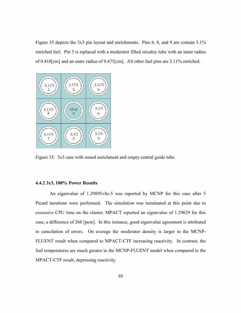
95
Figure 35 depicts the 3x3 pin layout and enrichments. Pins 6, 8, and 9 are contain 3.1%
enriched fuel. Pin 5 is replaced with a moderator filled zircaloy tube with an inner radius
of 0.418[cm] and an outer radius of 0.475[cm]. All other fuel pins are 2.11% enriched.
Figure 35: 3x3 case with zoned enrichment and empty central guide tube.
4.4.2 3x3, 100% Power Results
An eigenvalue of 1.29895±8e-5 was reported by MCNP for this case after 5
Picard iterations were performed. The simulation was terminated at this point due to
excessive CPU time on the cluster. MPACT reported an eigenvalue of 1.29629 for this
case, a difference of 266 [pcm]. In this instance, good eigenvalue agreement is attributed
to cancelation of errors. On average the moderator density is larger in the MCNP-
FLUENT result when compared to MPACT-CTF increasing reactivity. In contrast, the
fuel temperatures are much greater in the MCNP-FLUENT model when compared to the
MPACT-CTF result, depressing reactivity.

96
A normalized pin power comparison plot is given in Figure 36 for this case. The
MCNP-FLUENT model predicts peak power at a lower axial location than the MPACT-
CTF result. A maximum relative difference of 14.5% occurs at pin 4 at a location of
25[cm] from the inlet. Differences can be partially attributed to lower average moderator
densities in the immediate vicinity of the active pins at higher axial elevations in the
assembly. The lower density near the active pins is a symptom of poor moderator
mixing. In figure 37 the impact of poor flow mixing when compared to CTF is seen on
the moderator temperature profiles for each pin cell. The central channel is not heated,
and thus is contained in relatively high density, low temperature flow which does not
substantially migrate to the surrounding channels due to the absence of strong turbulent
mixing. The MPACT results suggest that the moderator experiences much more mixing
than predicted by the FLUENT model despite the absence of spacer grids.
Figure 36: Normalized pin power plot for 3x3 case. MPACT-CTF result shown as
broken black lines.
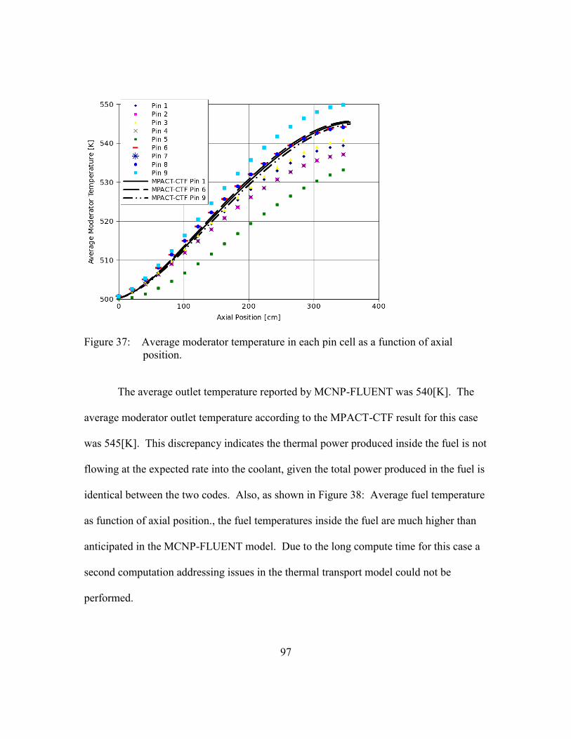
97
Figure 37: Average moderator temperature in each pin cell as a function of axial
position.
The average outlet temperature reported by MCNP-FLUENT was 540[K]. The
average moderator outlet temperature according to the MPACT-CTF result for this case
was 545[K]. This discrepancy indicates the thermal power produced inside the fuel is not
flowing at the expected rate into the coolant, given the total power produced in the fuel is
identical between the two codes. Also, as shown in Figure 38: Average fuel temperature
as function of axial position., the fuel temperatures inside the fuel are much higher than
anticipated in the MCNP-FLUENT model. Due to the long compute time for this case a
second computation addressing issues in the thermal transport model could not be
performed.

98
Figure 38: Average fuel temperature as function of axial position.
Figure 39: Energy deposition rate [W/m3] in the 3x3 assembly. 3.1% enriched pins are
in front.
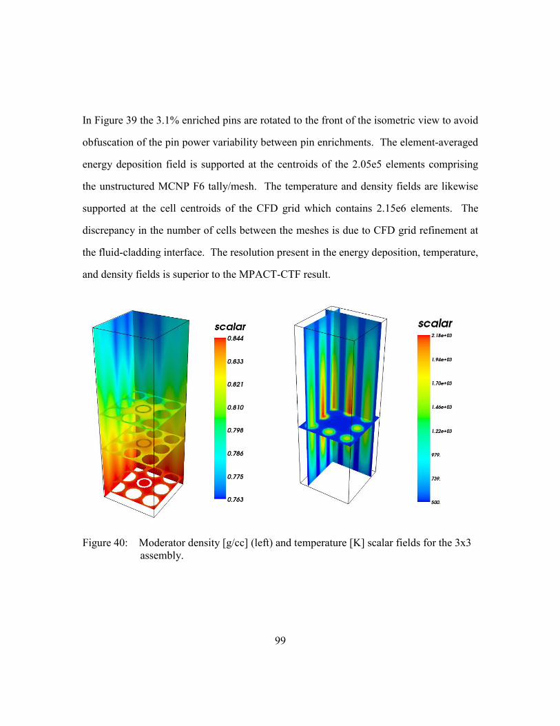
99
In Figure 39 the 3.1% enriched pins are rotated to the front of the isometric view to avoid
obfuscation of the pin power variability between pin enrichments. The element-averaged
energy deposition field is supported at the centroids of the 2.05e5 elements comprising
the unstructured MCNP F6 tally/mesh. The temperature and density fields are likewise
supported at the cell centroids of the CFD grid which contains 2.15e6 elements. The
discrepancy in the number of cells between the meshes is due to CFD grid refinement at
the fluid-cladding interface. The resolution present in the energy deposition, temperature,
and density fields is superior to the MPACT-CTF result.
Figure 40: Moderator density [g/cc] (left) and temperature [K] scalar fields for the 3x3
assembly.

100
In the moderator temperature plot given in Figure 40 the 3.1% enriched pins are located
furthest from the observer. The plot shows depression in the moderator density field
surrounding the high power, 3.1% enriched pins.
4.4.3 3x3 Pin Conclusions
The temperature field produced by MPACT-CTF differs significantly from the
result produced by the MCNP-FLUENT coupling. This difference is partially attributed
to a discrepancy in the degree of moderator mixing predicted between the CTF and
FLUENT models. In addition, the average moderator outlet temperature between the two
codes differed by 5[K], indicating the FLUENT computation did not obey energy
conservation. Addressing these issues in the thermal hydraulics model was not possible
due to exceptionally long compute times.
To complete 5 outer iterations for this problem consumed in excess of 19,000
CPU hours on 64 AMD Opteron 2.1GHz cores. This corresponds to a wall time of 12.5
days. In terms of number of F6 tally cells and number of distinct materials tracked by
MCNP the 3x3 pin configuration is approaching the limit of problem size tractable to the
MCNP-FLUENT coupling on the available computing equipment. The fidelity required
in the F6 heating tally in order to reduce aliasing error in the mapping of the volumetric
heating field to FLUENT precludes the user from coarsening the heating tally in an effort
to reduce runtimes. The FLUENT and mesh to mesh mapping runtimes were negligible
when compared to the MCNP runtime. Future improvements to the tally rendezvous and
particle tracking routines on unstructured meshes inside MCNP in addition to the the
availability of much larger computers could reduce run times.
101
4.5 SCALABILITY SUMMARY
In this section, CPU time results for MCNP are presented for a variety of cases.
CFD and overhead run times are omitted as the MCNP computation comprises >95% of
all computation time for all studied cases. Table 28 provides MCNP CPU times in
relation to the number of particles run and number of F6 tally elements. CPU time is
estimated as the number of cores multiplied by wall clock time. The timing results
include the setup and teardown time internal to the MCNP calculation. The setup time
includes the time required to build the F6 mesh from an ABAQUS unstructured mesh file
input and to setup communication between all MPI processes. Teardown time includes
the time to write results to the hard disk.

102
Table 28) MCNP timing results derived from unit cell, plane wall and full height single
fuel pin cases.
Picard
Iteration
# Mat
Cards
F6 Cells Particles/gen Total
Generations
Total
Particles
Run
CPU Time
[hrs]
Unit Cell
1 20 2000 5e4 220 1.1e7 133
1 20 3200 5e4 220 1.1e7 154
1 20 4400 5e4 220 1.1e7 172
Plane Wall
1 32 448 2e4 400 8.0e6 6
2 ↓ ↓ 2e4 800 1.6e7 12
3 ↓ ↓ 3e4 800 2.4e7 18
4 ↓ ↓ 4e4 800 3.2e7 25
5 ↓ ↓ 5e5 800 4.0e8 31
6 ↓ ↓ 5e5 1200 6.0e8 46
7 ↓ ↓ 5e5 1200 6.0e8 46
8 ↓ ↓ 5e5 1200 6.0e8 46
Full Height Pin Cell (quarter symmetry)
1 92 14776 3e4 400 1.2e7 145
2 ↓ ↓ 3e4 800 2.4e7 285
3 ↓ ↓ 3e4 800 2.4e7 287
4 ↓ ↓ 3e4 1000 3.0e7 358
5 ↓ ↓ 4e4 1000 4.0e7 358
6 ↓ ↓ 4e4 1200 4.8e7 430
7 ↓ ↓ 4e4 1500 6.0e7 712
8 ↓ ↓ 4e4 1500 6.0e7 712
9 ↓ ↓ 4e4 1500 6.0e7 712
3x3 Pin Assembly (full symmetry)
1 3170 208928 5e4 150 7.5e6 950
2 ↓ ↓ 7e4 300 2.1e7 2850
3 ↓ ↓ 8e4 500 4.0e7 2900
4 ↓ ↓ 1e5 500 5.0e7 5400
5 ↓ ↓ 2e5 500 1.0e8 6800

103
In addition to the number of F6 tally cells and total number of particles simulated, the
number of materials specified in the problem also increases the run time. A larger
number of materials demands a larger library of ACE cross sections be loaded into
memory. Given these three factors, the available timing data set is not large enough to
enable regression analyses to extrapolate run times outside of the investigated material,
F6 cell, and particle count range.
104
CHAPTER 5
Conclusion
The multiphysics coupling methods employed in this work successfully brought
together MCNP v.6.1 and ANSYS FLUENT v.14.0. The methodology allowed field data
to be passed between the two codes in an automated fashion. An under relaxed Picard
iteration scheme provided the multiphysics framework that guided the construction and
implementation of coupling routines. NJOY was employed to generate ACE formatted
Doppler broadened cross sections at specified 50K intervals which were utilized in a
pseudo material mixture routine. As discussed in section 3.1.4 Doppler Feedback, the
pseudo material mixing approach allowed the coupling methodology to account for the
effects of Doppler broadening on reactivity.
Excellent geometric and F6 tally generation flexibility was provided by
leveraging MCNP v6’s unstructured meshing capability. In principle, any geometry that
can be drawn in a Computer Aided Design (CAD) software can be incorporated into the
MCNP and ANSYS FLUENT model. Geometry construction was performed by stacking
together individually meshed “parts” to create a complete problem assembly. The
number of individual parts corresponded to the number of distinct MCNP material
regions in the problem. Control of the size and type of mesh elements used in the F6
heating tally was made possible by harnessing the unstructured meshing capabilities of
MCNP and by adopting a highly flexible mesh generation program, in this instance
GMSH. This approach to problem construction enables the methods put forth in this
thesis to be applied in cases where voxelization of organic, complicated geometries is
required. Examples include advanced reactor fuel geometries, and dose computations
involving organic geometry.

105
The single pin case conducted with no thermal hydraulic feedback and no axially
dependence exercised MCNP’s unstructured mesh tally and geometry construction
capabilities. Eigenvalue agreement between MCNP-FLUENT and MPACT-CTF was
within 150 [pcm]. The influence of using a linear finite element representation of the
curved fuel pin geometry was quantified. Artificially expanding the fuel and moderator
regions in the finite element geometry such that fuel and moderator volumes were
preserved corrected reactivity differences.
The 2D plane wall configuration with thermal hydraulic feedbacks enabled
provided a test-bed for the coupling methodology. The number of particle histories
simulated per Picard iteration performed was shown to have a substantial impact on the
heating tally tolerance. A factor of two decrease in the magnitude of local power
fluctuations was shown to require a factor of two increase in the total number of particle
histories run.
Comparisons with MPACT-CTF for the single pin case with thermal hydraulic
feedbacks yielded maximum power profile discrepancies of 4.0% at both the 75% and
100% power conditions. Eigenvalue agreements of 355[pcm] were achieved. In the 3x3
assembly, a lack of turbulent mixing and issues with energy conservation lead to large
discrepancies between the MCNP-FLUENT and MPACT-CTF solutions. A compute
time of 12.5 days for this case precluded additional coupled runs from being performed
for this case. Qualitatively correct trends in the power profiles due to varied enrichments
were predicted by MCNP-FLUENT, however. With this case, the ability to produce
results on a 2e6 element CFD mesh and a 2e5 element F6 tally was demonstrated on
modest computer hardware.
Challenges remain to be overcome as development of MCNP-FLUENT’s
coupling capabilities continues. The outer loop convergence rate in MCNP-FLUENT is

106
diminished by Monte Carlo noise; however under-relaxation was shown to dampen
statistical jitter and to facilitate convergence of Picard iterations. In future work, an
optimal under relaxation strategy similar to the method outlined in section 3.1.6, akin to
Anderson acceleration, could be implemented to further improve the convergence rate.
However, such an implementation of an optimal relaxation scheme is not straightforward
due to the presence of Monte Carlo noise introduced in the solution vector by MCNP. It
is not expected that Anderson acceleration could be used directly in the case of Monte
Carlo radiation transport - CFD coupling applications. Previous work on Anderson
acceleration can be used as a starting point for the development of a generalized strategy
for optimally choosing weighting coefficients in order to dampen power oscillations.
Improvements in the mesh to mesh solution mapping techniques are possible.
Utilizing a higher order interpolation scheme would reduce the aliasing error incurred
when mapping the F6 heating tally to the CFD grid. Data Transfer Kit (DTK) can
provide the necessary tools to reduce this aliasing error. DTK is a C++ library designed
to perform solution mapping between computational grids. DTK offers locally
conservative interpolation schemes for point cloud (mesh-free) data representations by
leveraging compactly supported radial basis functions [31]. In order to utilize DTK in
the current implementation, DTK interfaces must be developed for MCNP and ANSYS
FLUENT. The custom interfaces would then be wrapped in Python.
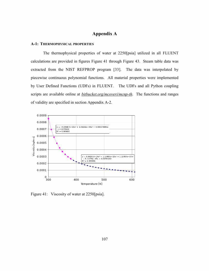
107
Appendix A
A-1: THERMOPHYSICAL PROPERTIES
The thermophysical properties of water at 2250[psia] utilized in all FLUENT
calculations are provided in figures Figure 41 through Figure 43. Steam table data was
extracted from the NIST REFPROP program [33]. The data was interpolated by
piecewise continuous polynomial functions. All material properties were implemented
by User Defined Functions (UDFs) in FLUENT. The UDFs and all Python coupling
scripts are available online at bitbucket.org/mcoveri/mcnp-th. The functions and ranges
of validity are specified in section Appendix A-2.
Figure 41: Viscosity of water at 2250[psia].

108
Figure 42: Density of water at 2250[psia].
Figure 43: Isobaric specific heat of water at 2250[psia].
Thermophysical properties of Uranium oxide and Helium fill gas were obtained from
[34]. The UDF code is provided in section A-2. In addition to material properties, the
UDF code contains the subroutine DEFINE_SOURCE which is required to allocate a
109
user defined scalar (UDS) field inside FLUENT so that a custom volumetric heat source
may be read, interpolated, and stored as a solution variable.
A-2: UDF CODE /**************** FLUENT UDF ********************/
#include "udf.h"
// H2O PROPS at 2250 psia
DEFINE_PROPERTY(H2O_density, cell, thread)
{
real t, rho;
t = C_T(cell, thread);
// w / m K
if (t < 300.)
{
rho = 1003.4;
}
else if (t < 618.01)
{
rho = -6.95709e-8*pow(t,4.)+1.17907e-4*pow(t,3.)-7.61556e-2*pow(t,2.)+21.2884*t-1151.26;
}
else
{
rho = 594.13;
}
return rho;
}
DEFINE_PROPERTY(H2O_solid_density, cell, thread)
{
real t, rho;
t = C_T(cell, thread);
// w / m K
if (t < 300.)
{
rho = 1003.4;
}
else if (t < 618.01)
{
rho = -6.95709e-8*pow(t,4.)+1.17907e-4*pow(t,3.)-7.61556e-2*pow(t,2.)+21.2884*t-1151.26;
}
else
{
rho = 594.13;
}
return rho;
}
DEFINE_PROPERTY(H2O_viscosity, cell, thread)
{
real t, mu;
t = C_T(cell, thread);
// w / m K
if (t < 380.)
{
mu = -9.09487e-10*pow(t, 3.)+1.01182e-6*pow(t, 2.)-3.78494e-4*t+0.0478904;
}
else
{
mu = 6.66161e-14*pow(t, 4.)-1.53465e-10*pow(t, 3.)+1.32487e-7*pow(t, 2.)-5.12276e-
5*t+7.63282e-3;
}
return mu;
}
DEFINE_SPECIFIC_HEAT(H2O_cp, t, Tref, h, yi)
{
110
real cp;
// real hRef;
// hRef = 0.0; // enthalpy at ref T of 298.15K
// j / mol K -> j / kg K
if (t < 460.)
{
cp = 6.7314e-8*pow(t, 4.)-5.94628e-5*pow(t, 3.)+0.0191488*pow(t, 2.)-2.40736*t+4198.27;
*h = (1./5.)*6.7314e-8*pow(t, 5.)-(1./4.)*5.94628e-5*pow(t, 4.)+(1./3.)*0.0191488*pow(t, 3.)
-(1./2.)*2.40736*pow(t, 2.)+4198.27*t
- ((1./5.)*6.7314e-8*pow(Tref, 5.)-(1./4.)*5.94628e-5*pow(Tref,
4.)+(1./3.)*0.0191488*pow(Tref, 3.)
-(1./2.)*2.40736*pow(Tref, 2.)+4198.27*Tref);
}
else if (t < 618.01)
{
cp = 7.29113e-6*pow(t, 4.)-1.43767e-2*pow(t, 3.)+10.6559*pow(t, 2.)-3512.65*t+438300;
*h = (1./5.)*7.29113e-6*pow(t, 5.)-(1./4.)*1.43767e-2*pow(t, 4.)
+(1./3.)*10.6559*pow(t, 3.)-(1./2.)*3512.65*pow(t, 2.)+438300*t
- ((1./5.)*7.29113e-6*pow(Tref, 5.)-(1./4.)*1.43767e-2*pow(Tref, 4.)
+(1./3.)*10.6559*pow(Tref, 3.)-(1./2.)*3512.65*pow(Tref, 2.)+438300*Tref);
}
else
{
cp = 7.29113e-6*pow(618.01, 4.)-1.43767e-2*pow(618.01, 3.)+10.6559*pow(618.01, 2.)-
3512.65*618.01+438300;
*h = (1./5.)*7.29113e-6*pow(618.01, 5.)-(1./4.)*1.43767e-2*pow(618.01, 4.)
+(1./3.)*10.6559*pow(618.01, 3.)-(1./2.)*3512.65*pow(618.01, 2.)+438300*618.01
- ((1./5.)*7.29113e-6*pow(Tref, 5.)-(1./4.)*1.43767e-2*pow(Tref, 4.)
+(1./3.)*10.6559*pow(Tref, 3.)-(1./2.)*3512.65*pow(Tref, 2.)+438300*Tref);
}
return cp;
}
// UO2 PROPS
DEFINE_PROPERTY(UO2_conductivity, cell, thread)
{
real t, k1;
t = C_T(cell, thread) / 1000.;
// w / m K
k1 = 100. / (7.5408 + 17.692*t + 3.6142*pow(t, 2.)) + 6400. / pow(t, 5./2.) * exp(-16.35/t);
return k1;
}
DEFINE_SPECIFIC_HEAT(UO2_cp, t, Tref, h, yi)
{
real cp;
real m;
real TT;
real TTref;
// real hRef;
// hRef = 0.0; // enthalpy at ref T of 298.15K
m = 270.0e-3; // kg / mol
TT = t/1000.;
TTref = Tref/1000.;
// j / mol K -> j / kg K
cp = (1./m) * (52.1743 + 87.951*(TT) - 84.2411*pow((TT), 2.) + 31.542*pow((TT), 3.) -
2.6334*pow((TT), 4.) - 0.71391*pow((TT), -2.));
*h = (1./m) * (
-21.1762 + 52.1743*TT + 43.9753*pow(TT, 2.) - 28.0804*pow(TT, 3.) + 7.88552*pow(TT, 4.)
- 0.52668*pow(TT, 5.) + 0.71391*pow(TT, -1.)
- ( -21.1762 + 52.1743*TTref + 43.9753*pow(TTref, 2.) - 28.0804*pow(TTref, 3.) +
7.88552*pow(TTref, 4.)
- 0.52668*pow(TTref, 5.) + 0.71391*pow(TTref, -1.))
);
return cp;
}
// ZIRC-2 PROPS
DEFINE_PROPERTY(zirc_conductivity, cell, thread)
{
real t, k1;
t = C_T(cell, thread);
// w / m K
k1 = 12.767 - 5.4348e-4*t + 8.9818e-6*pow(t, 2.);
return k1;

111
}
DEFINE_SPECIFIC_HEAT(zirc_cp, t, Tref, h, yi)
{
real cp;
// real hRef;
// hRef = 0.0; // enthalpy at ref T of 298.15K
// j / kg K
cp = 255.66 + 0.1024*t;
*h = 255.66*t + (1./2.)*0.1024*pow(t, 2.)
- (255.66*Tref + (1./2.)*0.1024*pow(Tref, 2.));
//*h = cp*(t-Tref);
return cp;
}
// He PROPS
DEFINE_PROPERTY(he_conductivity, cell, thread)
{
real t, k1;
t = C_T(cell, thread);
// w / m K
// k1 = -5.84419e-8*pow(t, 2.) + 3.66895e-4*t + 5.38251e-2; // He Prop
k1 = 0.4769772; // assuming gap of 0.0084 cm and h of 5678.3 W / m k
return k1;
}
DEFINE_PROPERTY(he_density, cell, thread)
{
real t, rho;
t = C_T(cell, thread);
// kg/m3
rho = 1.27027e-7*pow(t, 2.) - 3.15058e-4*t + 0.230879;
return rho;
}
DEFINE_SOURCE(vol_heat_source, cell, thread, dS, eqn)
{
real source;
source = C_UDSI(cell, thread, 0);
return source;
}/**************** END FLUENT UDF ********************/

112
Bibliography
[1] J.R. Haines, et. al. Spallation neutron source target station design, development, and
commissioning. Nuclear Instruments and Methods in Physics Research
Section A: Accelerators, Spectrometers, Detectors and Associated
Equipment. Volume 764, 11 November 2014, Pages 94–115
[2] Cold Neutron Source. ANSTO. Web. 23 Nov. 2015. http://www.ansto.gov.au/
[3] S.I., WU, and KIM Y.K. INSTALLATION OF COLD NEUTRON SOURCE AT
HANARO. Korea Atomic Energy Research Institute (KAERI).
http://www-
pub.iaea.org/MTCD/Publications/PDF/P1575_CD_web/datasets/papers/
A25%20Wu.pdf
[4] Technische Univ. Muenchen (Germany); Framatome ANP GmbH, Erlangen
(Germany). Intense positron source at the Munich research reactor
FRM-II. Meeting of the International Group on Research Reactors
(IGORR). Munich (Germany). 17-20 Apr 2001.
[5] B. Kochunas. D. Jabayy. T. Downar. VERA Problem 10: Restart and Shuffling in
MPACT. CASL-U-2014-0231-001. February 2015.
www.casl.gov/docs/ CASL-U-2014-0231-001.pdf
[6] T. S. Blyth. Improvement of COBRA-TF Subchannel Thermal-Hydraulics Code
(CTF) using CFD. CASL-U-2015-0020-000. December 2014.
www.casl.gov/docs/CASL-U-2015-0020-000.pdf
[7] B. Collins, et. al. Demonstration of Full Core Reactor Depletion with MPACT.
CASL-U-2014-0140-000. 2014. www.casl.gov/docs/ CASL-U-2014-
0140-000.pdf
[8] S. Palmtag, A. Godfrey. User Manual for the VERA Input Processor. CASL-U-
2014-0014-002. 2015. www.casl.gov/docs/CASL-U-2014-0014-
002.pdf
[9] Neutronics and CFD Analysis: MCNPX-ANSYS Fluent Coupling. Idom Nuclear
Services. April 2013.
[10] C. Hughes, K. Jordan, D. Schubring. Coupled Computational Heat Transfer and
Reactor Physics for SCWR. Proceedings from the ASME Heat Transfer
Summer Conference. 2013.

113
[11] J.L. Collins. et al. Pseudo Material Construct for Coupled Neutronic-Thermal-
Hydraulic Analysis of VHTGR. Transactions of the American Nuclear
Society. 2005.
[12] Jianwei, Hu, and Rizwan-uddin. "Coupled Neutronics and Thermal-Hydraulics
Simulations Using MCNP and FLUENT." Advancements in Multi-
Physics Reactor Simulation, 2008.
[13] Cardoni, Jeffery. Thesis: NUCLEAR REACTOR MULTI-PHYSICS
SIMULATIONS WITH COUPLED MCNP5 AND STAR-CCM+. U of
Illinois at Urbana-Champaign, 2011.
[14] J. Yan, B. Kochunas, M. Hursin, T. Downar, Z. Karoutas. Coupled Computational
Fluid Dynamics and MOC Neutronic Simulations of Westinghouse
PWR Fuel Assemblies with Grid Spaces. 14th
International Topical
Meeting on Nuclear Reactor Thermalhydraulics, NURETH14-254.
2011.
[15] V. Seker, J.W. Thomas, T. Downar. Reactor Physics Simulation with Coupled
Monte Carlo Calculations and Computational Fluid Dynamics.
International Conference on Emerging Nuclear Energy Systems
(ICENES). 2007.
[16] Lewis, E. E., and W. F. Miller. Computational Methods of Neutron Transport. La
Grange Park, IL, USA: American Nuclear Society, 1993.
[17] Yun, Sunghwan, and Nam Zin Cho. "Acceleration of Source Convergence in Monte
Carlo K-eigenvalue Problems via Anchoring with a P-CMFD
Deterministic Method." Annals of Nuclear Energy 37.12, 2010: 1649-
658.
[18] MCNP6 Users Manual - Code Version 6.1.1beta, LA-CP-14-00745. June 2014.
[19] R.L. Martz. The MCNP6 Book on Unstructured Mesh Geomerty: User's Guide.
LA-UR-11-05668-rev8. 2014.
[20] ANSYS INC. "Fluent 14 Theory Guide." 2009.
[21] S. Patankar. Numerical Heat Transfer and Fluid Flow. CRC Press, 1980.

114
[22] C. Geuzaine and J.-F. Remacle. Gmsh: a three-dimensional finite element mesh
generator with built-in pre- and post-processing facilities. International
Journal for Numerical Methods in Engineering 79(11), pp. 1309-1331.
2009.
[23] SciPy Reference guide v 0.14.0. The Scipy Community. http://www.scipy.org
[24] Macfarle et al. The NJOY Nuclear Data Processing System: User’s Manual. Los
Alamos USA. 1993.
[25] R. Stammler and M. Abbate, Methods of Steady-State Reactor Physics in Nuclear
Design, Academic Press 1983.
[26] R. Pawlowski, R. Bartlett, N. Belcourt, N. Hooper. R. Schmidt. A Theory Manual
for Multi-Physics Code Coupling in LIME. Sandia National Laboritory.
SAND2011-2195. 2011.
[27] Kelley, C.T., and A.R. Toth. Convergence Analysis for Anderson Acceleration.
Society for Industrial and Applied Mathematics (SIAM) Journal on
Numerical Analysis (SINUM), November 13, 2014.
[28] Toth, A.R., C.T. Kelley, S.R. Slattery, S.P. Hamilton and K.T. Clarno, "Analysis of
Anderson Acceleration on a Simplified Neutronics/Thermal Hydraulics
System," Proceedings of the ANS MC2015 - Joint International
Conference on Mathematics and Computation (M&C), Supercomputing
in Nuclear Applications (SNA) and the Monte Carlo (MC) Method,
Volume ANS MC2015 CD, April 19, 2015, Nashville, Tennessee, 2015.
[29] Godfrey, A., VERA Core Physics Benchmark Progression Problem Specifications,
Revision 4, CASL Technical Report: CASL-U-2012-0131-004, August
29, 2014.
[30] Munson, Bruce Roy, T. H. Okiishi, and Wade W. Huebsch. Fundamentals of Fluid
Mechanics. Wiley & Sons, 2009.
[31] S. R. Slattery. Mesh-Free Data Transfer Algorithms for Partitioned Multiphysics
Problems: Conservation, Accuracy and Parallelism. CASL-U-2014-
0128-000. 2014. http://www.casl.gov/docs/ CASL-U-2014-0128-
000.pdf
[32] R. Salko, M. Avramova. COBRA-TF Subchannel Thermal Hydraulics Code (CTF)
Manual. CASL-U-2015-0054-000. 2015.

115
[33] Eric. W. Lemmon, Marica L. Huber, Mark O. McLinden. REFPROP User Guide.
NIST, 2007. http://www.nist.gov/srd/upload/REFPROP8.PDF
[34] Thermophysical Properties Database for Light Water Reactors and Heavy Water
Reactors. IAEA-TECDOC-1496. 2006.
[35] Jin, M., and M. Short, Two-Phase Fluid Flow Modeling in CRUD using MAMBA-
BDM, CASL Technical Report CASL-U-2014-0143-000, February 17,
2014.