Front-door Difference-in-Differences Estimators · Front-door Difference-in-Differences Estimators*...
40
Front-door Difference-in-Differences Estimators * Adam Glynn † Konstantin Kashin ‡ [email protected] [email protected] June 12, 2014 Abstract In this paper, we develop front-door difference-in-differences estimators that utilize infor- mation from post-treatment variables in addition to information from pre-treatment covariates. Even when the front-door criterion does not hold, these estimators allow the identication of causal effects under assumptions related to standard difference-in-differences assumptions and allow the bounding of causal effects under relaxed assumptions. We illustrate these points with an application to the National JTPA (Job Training Partnership Act) Study and with an applica- tion to Florida’s early in-person voting program. For the JTPA study, we show that an experi- mental benchmark can be bracketed with front-door and front-door difference-in-differences estimates. Surprisingly, neither of these estimates use control units. For the Florida program, we nd some evidence that early in-person voting had small positive effects on turnout in 2008 and 2012. is provides a counterpoint to recent claims that early voting had a negative effect on turnout in 2008. *We thank Barry Burden, Justin Grimmer, Manabu Kuroki, Kevin Quinn, and seminar participants at Emory, Harvard, Notre Dame, NYU, Ohio State, UC Davis, and UMass Amherst for comments and suggestions. Earlier versions of this paper were presented at the 2014 MPSA Conference and the 2014 Asian Political Methodology Meeting in Tokyo. †Department of Political Science, Emory University, 327 Tarbutton Hall, 1555 Dickey Drive, Atlanta, GA 30322 (http://scholar.harvard.edu/aglynn). ‡Department of Government and Institute for Quantitative Social Science, Harvard University, 1737 Cambridge Street, Cambridge, MA 02138 (http://konstantinkashin.com). 1
Transcript of Front-door Difference-in-Differences Estimators · Front-door Difference-in-Differences Estimators*...
Front-door Difference-in-Differences Estimators*
Adam Glynn† Konstantin Kashin‡
[email protected] [email protected]
June 12, 2014
Abstract
In this paper, we develop front-door difference-in-differences estimators that utilize infor-mation frompost-treatment variables in addition to information frompre-treatment covariates.Even when the front-door criterion does not hold, these estimators allow the identi cation ofcausal effects under assumptions related to standard difference-in-differences assumptions andallow the bounding of causal effects under relaxed assumptions. We illustrate these points withan application to the National JTPA (Job Training Partnership Act) Study and with an applica-tion to Florida’s early in-person voting program. For the JTPA study, we show that an experi-mental benchmark can be bracketed with front-door and front-door difference-in-differencesestimates. Surprisingly, neither of these estimates use control units. For the Florida program,we nd some evidence that early in-person voting had small positive effects on turnout in 2008and 2012. is provides a counterpoint to recent claims that early voting had a negative effecton turnout in 2008.
*We thank Barry Burden, Justin Grimmer, Manabu Kuroki, Kevin Quinn, and seminar participants at Emory,Harvard, NotreDame, NYU,Ohio State, UCDavis, andUMassAmherst for comments and suggestions. Earlier versionsof this paper were presented at the 2014MPSAConference and the 2014Asian PoliticalMethodologyMeeting in Tokyo.
†Department of Political Science, Emory University, 327 Tarbutton Hall, 1555 Dickey Drive, Atlanta, GA 30322(http://scholar.harvard.edu/aglynn).
‡Department of Government and Institute for Quantitative Social Science, Harvard University, 1737 CambridgeStreet, Cambridge, MA 02138 (http://konstantinkashin.com).
1
1 Introduction
One of the main tenets of observational studies is that post-treatment variables should not be in-
cluded in an analysis because naively conditioning on these variables can block some of the effect
of interest, leading to post-treatment bias (King, Keohane and Verba, 1994). While this is usually
sound advice, it seems to contradict recommendations from the process tracing literature that in-
formation about mechanisms can be used to assess the plausibility of an effect (Collier and Brady,
2004; George and Bennett, 2005; Brady, Collier and Seawright, 2006).
e front-door criterion (Pearl, 1995) and its extensions (Kuroki and Miyakawa, 1999; Tian and
Pearl, 2002a,b; Shpitser and Pearl, 2006) resolve this apparent contradiction, providing a means for
nonparametric identi cation of treatment effects using post-treatment variables. Importantly, the
front-door approach can identify causal effects even when there are unmeasured common causes
of the treatment and the outcome (i.e., the total effect is confounded). However, the front-door ad-
justment has been used infrequently (VanderWeele, 2009) due to concerns that the assumptions re-
quired for point identi cation will rarely hold (Cox and Wermuth, 1995; Imbens and Rubin, 1995).
A number of papers have proposed weaker and more plausible sets of assumptions (Joffe, 2001;
Kaufman, Kaufman andMacLehose, 2009; Glynn andQuinn, 2011) that tend to correspond to con-
ceptions of process tracing. However, these approaches rely on binary or bounded outcomes, and
even in large samples these methods only provide bounds on causal effects (i.e., partial instead of
point identi cation). Additionally, these bounds on effects typically include zero. Recently, Glynn
and Kashin (2013) developed bias formulas that allow the front-door assumptions to be weakened
via sensitivity analysis. is allows for any type of outcome variable and increases the possibility
that the front-door approach will be informative (e.g., establishing that zero is not a plausible value
for the effect). In this paper, we demonstrate that the bias described in Glynn and Kashin (2013)
can sometimes be removed by a difference-in-differences approach when there is one-sided non-
compliance. Glynn and Kashin (2013) showed that with one-sided noncompliance, the front-door
2

estimator implies substituting treated noncompliers for controls. For example, if you want to study
the effect of signing up for a program, the front-door estimator compares the outcomes of those that
sign up (the treated) to the subset of those that sign up but do not show up (the treated noncompli-
ers). Contrast this with standard approaches (e.g., matching and regression) that would compare
those that sign up (the treated) with those that do not sign up (the controls).
e front-door difference-in-differences approach extends the front-door approach in the fol-
lowing manner. First, we identify the treated units of interest, which we will refer to as the group of
interest. Second, if we can identify a group of treated units distinct from our group of interest for
which we believe the treatment should have no effect, then a non-zero front-door estimate for this
group can be attributed to bias. We will refer to this group as the differencing group. For example,
in the context of the early voting application to follow, we consider the effects of an early in-person
(EIP) voting program on turnout for elections in 2008 and 2012. One differencing group we con-
sider is potential voters that used an absentee ballot in the previous election. EIP was unlikely to
have an effect on these voters, as they had already demonstrated their ability to vote by another
means of early voting. erefore, we consider non-zero front-door estimates of the turnout effect
for this group to be evidence of bias.
If we further assume that the bias for the differencing group is equal to the bias for our group of
interest, then by subtracting the front-door estimator for this group from the front-door estimator
for the group of interest, we can remove the bias from our front-door estimate for the group of
interest. Note that if all effects and bias are positive, then when the bias from the differencing group
is larger than the bias for the group of interest and/or the treatment has an effect for the differencing
group, then this differencing approach can provide a lower bound on the effect of the program. We
demonstrate this within the context of a job training study. However, we also demonstrate that the
bias for each group is related to the proportion of compliers in the group, and therefore, an equal bias
assumption is untenable without an additional adjustment. is will be described in detail below.
e paper is organized as follows. Section 2 presents the bias formulas for the front-door ap-
3
proach to estimating average treatment effects on the treated (ATT), both for the general case and
the simpli cation for nonrandomized program evaluations with one-sided noncompliance. Sec-
tion 3 presents the difference-in-differences approach for front-door estimators for the simpli ed
case and discusses the required assumptions. Section 4 presents an application of the front-door
difference-in-differences estimator to the National JTPA (Job Training Partnership Act) Study. Sec-
tion 5 presents an application of the front-door difference-in-differences estimator to election law:
assessing the effects of early in-person voting on turnout in Florida. Section 6 concludes.
2 Bias for the Front-Door Approach for ATT
In this section, we present large-sample bias formulas for the front-door approach for estimating the
average treatment effect on the treated (ATT). is is oen the parameter of interest when assessing
the effects of a program or a law. For an outcome variable Y and a binary treatment/action A, we
de ne the potential outcome under active treatment as Y(a1) and the potential outcome under con-
trol as Y(a0). Our parameter of interest is the ATT, de ned as τatt = E[Y(a1)|a1] − E[Y(a0)|a1] =
μ1|a1− μ0|a1
. We assume consistency, E[Y(a1)|a1] = E[Y|a1], so that the mean potential outcome
under active treatment for the treated units is equal to the observed outcome for the treated units
such that τatt = E[Y|a1] − E[Y(a0)|a1]. e ATT is therefore the difference between the mean out-
come for the treated units and mean counterfactual outcome for these units, had they not received
the treatment.
We also assume that μ0|a1is potentially identi able by conditioning on a set of observed co-
variates X and unobserved covariates U. To clarify, we assume that if the unobserved covariates
were actually observed, the ATT could be estimated by standard approaches (e.g., matching). For
Note that we must assume that these potential outcomes are well de ned for each individual,
and therefore we are making the stable unit treatment value assumption (SUTVA).
4
simplicity in presentation we assume that X and U are discrete, such that
μ0|a1=
∑x
∑u
E[Y|a0, x, u] · P(u|a1, x) · P(x|a1),
but continuous variables can be handled analogously. However, even with only discrete variables
we have assumed that the conditional expectations in this equation are well-de ned, such that for
all levels of X andU amongst the treated units, all units had a positive probability of receiving either
treatment or control (i.e., positivity holds).
e front-door adjustment for a set of measured post-treatment variables M can be written as
the following:
μfd0|a1=
∑x
∑m
P(m|a0, x) · E[Y|a1,m, x] · P(x|a1).
We can thus de ne the large-sample front-door estimator of ATT as:
τfdatt = μ1|a1− μfd0|a1
.
e large-sample bias in the front-door estimate of ATT, which is entirely attributable to the bias in
the front-door estimate of μ0|a1, is the following (see Appendix A.1 for a proof):
Bfdatt =
∑x
P(x|a1)∑m
∑u
P(m|a0, x, u) · E[Y|a0,m, x, u] · P(u|a1, x)
−∑x
P(x|a1)∑m
∑u
P(m|a0, x) · E[Y|a1,m, x, u] · P(u|a1,m, x).
As the bias formula shows, it is possible for the front-door approach to provide a large-sample
unbiased estimator for the ATT even in the presence of an unmeasured confounder that would
bias traditional covariate adjustment techniques such as matching and regression. Speci cally, the
front-door bias will be zero when three conditions hold: (1) E[Y|a1,m, x, u] = E[Y|a0,m, x, u], (2)
5
P(m|a0, x) = P(m|a0, x, u), and (3) P(u|a1,m, x) = P(u|a1, x). e rst will hold when Y is mean
independent of A conditional on U, M, and X, while the latter two will hold if U is independent of
M conditional on X and a0 or a1. is is an alternative derivation of the result from (Pearl, 1995),
although we focus on ATT instead of ATE and do not require the de nition of potential outcomes
beyond those required for the de nition of ATT.
For the difference-in-differences estimators we consider in this paper, we use the special case
of nonrandomized program evaluations with one-sided noncompliance. Following the literature in
econometrics on program evaluation, we de ne the program impact as the ATT where the active
treatment (a1) is assignment into a program (Heckman, LaLonde and Smith, 1999), and when M
indicates whether the active treatment (a1) was actually received. We use the short-hand notation
m1 to denote that active treatment was received and m0 if it was not.
Assumption 1 (One-sided noncompliance)
P(m0|a0, x) = P(m0|a0, x, u) = 1 for all x, u.
Assumption 1 implies that only those assigned to treatment can receive treatment, and the front-
door large-sample estimator reduces to the following under this assumption:
τfdatt = μ1|a1− μfd0|a1
= E[Y|a1]−∑x
∑m
P(m|a0, x) · E[Y|a1,m, x] · P(x|a1)
= E[Y|a1]−∑x
E[Y|a1,m0, x]︸ ︷︷ ︸treated non-compliers
·P(x|a1) (1)
=∑x
P(x|a1) · P(m1|x, a1) ·
E[Y|a1,m1, x]− E[Y|a1,m0, x]︸ ︷︷ ︸“effect” of receiving treatment
(2)
e formulas in (1) and (2) are interesting because they do not rely upon outcomes of control units
in the construction of proxies for the potential outcomes under control for treated units (see Ap-
pendix A.2 for the derivation of (2)). is is a noteworthy point that has implications for research
6
design that we will revisit subsequently. e formula in (1) can be compared to the standard large-
sample covariate adjustment for ATT:
τstdatt = μ1|a1− μstd0|a1
= E[Y|a1]−∑x
E[Y|a0, x]︸ ︷︷ ︸controls
·P(x|a1). (3)
Roughly speaking, standard covariate adjustment matches units that were assigned treatment to
similar units that were assigned control. On the other hand, front-door estimates match units that
were assigned treatment to similar units that were assigned treatment but did not receive treatment.
is sort of comparison is not typical, so it is helpful to consider the informal logic of the procedure
before presenting the formal statements of bias. e fundamental question is whether the treated
noncompliers provide reasonable proxies for the missing counterfactuals: the outcomes that would
have occurred if the treated units had not been assigned treatment. erefore, in order for the front-
door approach to be unbiased in large samples, we are effectively assuming that 1) assignment to
treatment has no effect if treatment is not received and 2) those that are assigned but don’t receive
treatment are comparable in some sense to those that receive treatment. is will be made more
precise below.
e front-door formula in (2), with the observable proportions P(x|a1) and P(m1|a1, x) mul-
tiplying the estimated effect of receiving the treatment, is helpful when considering the simpli ed
front-door ATT bias, which can be written in terms of the same observable proportions (see Ap-
pendices A.3 and A.4 for proofs):
Bfdatt =∑x
P(x|a1)P(m1|a1, x)∑u
[E[Y|a0,m0, x, u] · [P(u|a1,m1, x)− P(u|a1,m0, x)]
+{E[Y(a0)|a1,m1, x, u]
P(m1|a1, x, u)P(m1|a1, x)
− E[Y(a0)|a1,m0, x, u] ·E[Y|a1,m0,x,u]
E[Y(a0)|a1,m0,x,u] − P(m0|a1, x, u)P(m1|a1, x)
}· P(u|a1,m0, x)
]
e unobservable portion of this bias formula (i.e., everything aer the∑
u), can be difficult to
7
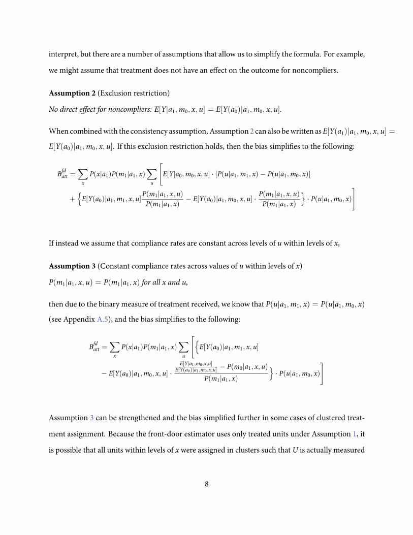
interpret, but there are a number of assumptions that allow us to simplify the formula. For example,
we might assume that treatment does not have an effect on the outcome for noncompliers.
Assumption 2 (Exclusion restriction)
No direct effect for noncompliers: E[Y|a1,m0, x, u] = E[Y(a0)|a1,m0, x, u].
When combinedwith the consistency assumption, Assumption 2 can also bewritten asE[Y(a1)|a1,m0, x, u] =
E[Y(a0)|a1,m0, x, u]. If this exclusion restriction holds, then the bias simpli es to the following:
Bfdatt =∑x
P(x|a1)P(m1|a1, x)∑u
[E[Y|a0,m0, x, u] · [P(u|a1,m1, x)− P(u|a1,m0, x)]
+{E[Y(a0)|a1,m1, x, u]
P(m1|a1, x, u)P(m1|a1, x)
− E[Y(a0)|a1,m0, x, u] ·P(m1|a1, x, u)P(m1|a1, x)
}· P(u|a1,m0, x)
]
If instead we assume that compliance rates are constant across levels of u within levels of x,
Assumption 3 (Constant compliance rates across values of u within levels of x)
P(m1|a1, x, u) = P(m1|a1, x) for all x and u,
then due to the binary measure of treatment received, we know that P(u|a1,m1, x) = P(u|a1,m0, x)
(see Appendix A.5), and the bias simpli es to the following:
Bfdatt =∑x
P(x|a1)P(m1|a1, x)∑u
[{E[Y(a0)|a1,m1, x, u]
− E[Y(a0)|a1,m0, x, u] ·E[Y|a1,m0,x,u]
E[Y(a0)|a1,m0,x,u] − P(m0|a1, x, u)P(m1|a1, x)
}· P(u|a1,m0, x)
]
Assumption 3 can be strengthened and the bias simpli ed further in some cases of clustered treat-
ment assignment. Because the front-door estimator uses only treated units under Assumption 1, it
is possible that all units within levels of x were assigned in clusters such that U is actually measured
8

at the cluster level. We present an example of this in the application, where treatment (the availabil-
ity of early in-person voting) is assigned at the state level, and therefore all units within a state (e.g.,
Florida) have the same value of u. Formally, the assumption can be stated as the following:
Assumption 4 (u is constant among treated units within levels of x)
For any two units with a1 and covariate values (x, u) and (x′, u′), x = x′ ⇒ u = u′.
When Assumption 4 holds, the u notation is redundant, and can be removed from the bias formula
which simpli es as the following:
Bfdatt =∑x
P(x|a1)P(m1|a1, x){E[Y(a0)|a1,m1, x]− E[Y(a0)|a1,m0, x] ·
E[Y|a1,m0,x]E[Y(a0)|a1,m0,x] − P(m0|a1, x)
P(m1|a1, x)
}(4)
Finally, it can be instructive to consider the formula when both Assumption 2 and Assumption 4
hold. In this scenario, the remaining bias is due to an unmeasured common cause of the mediator
and the outcome.
Bfdatt =
∑x
P(x|a1)P(m1|a1, x){E[Y(a0)|a1,m1, x]− E[Y(a0)|a1,m0, x]}
In some applications, the bias Bfdatt may be small enough for the front-door estimator to provide
a viable approach. For others, we may want to remove the bias. In the next section, we discuss a
difference-in-differences approach to removing the bias.
3 Front-door Difference-in-Differences Estimators
If we de ne the front-door estimator within levels of a covariate x as τfdatt,x, then the front-door
estimator can be written as a weighted average of strata-speci c front-door estimators where the
9
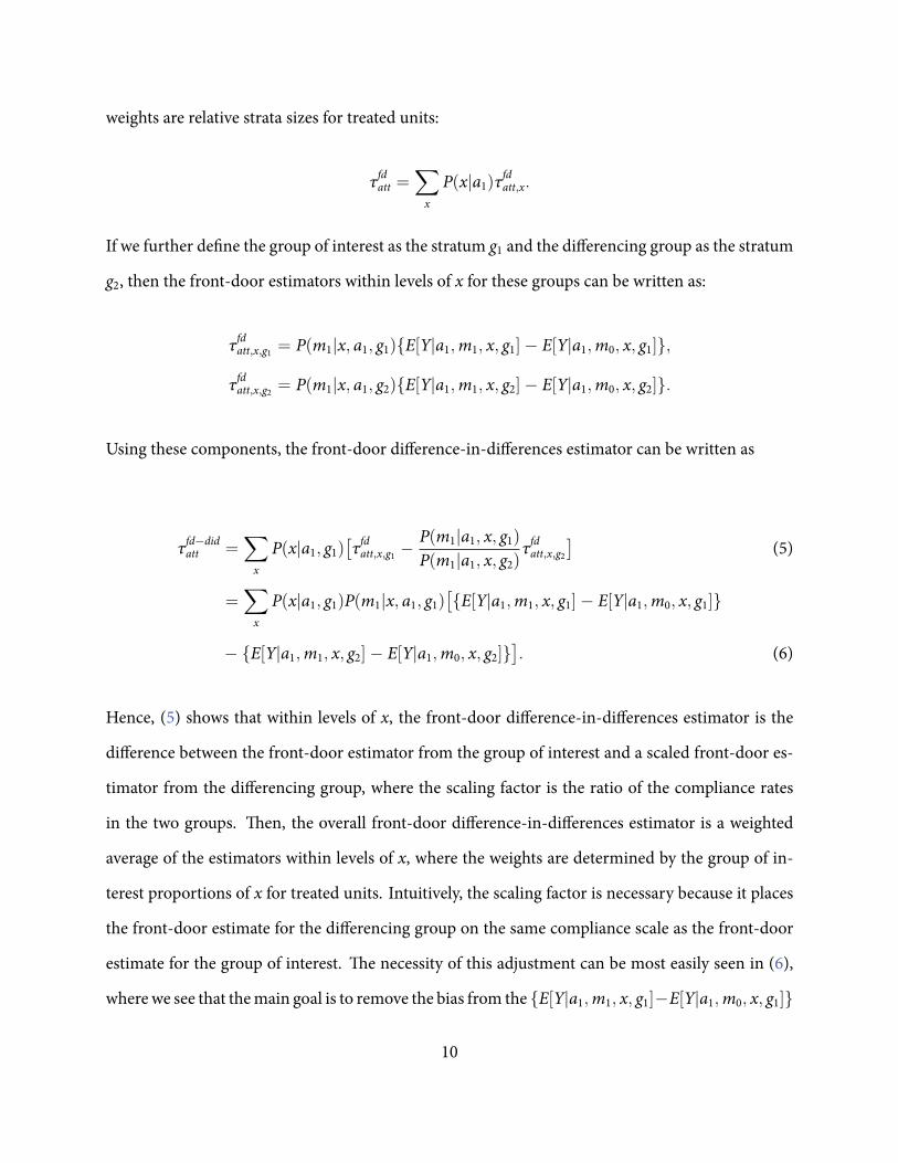
weights are relative strata sizes for treated units:
τfdatt =∑x
P(x|a1)τfdatt,x.
If we further de ne the group of interest as the stratum g1 and the differencing group as the stratum
g2, then the front-door estimators within levels of x for these groups can be written as:
τfdatt,x,g1 = P(m1|x, a1, g1){E[Y|a1,m1, x, g1]− E[Y|a1,m0, x, g1]},
τfdatt,x,g2 = P(m1|x, a1, g2){E[Y|a1,m1, x, g2]− E[Y|a1,m0, x, g2]}.
Using these components, the front-door difference-in-differences estimator can be written as
τfd−didatt =
∑x
P(x|a1, g1)[τfdatt,x,g1 −
P(m1|a1, x, g1)P(m1|a1, x, g2)
τfdatt,x,g2]
(5)
=∑x
P(x|a1, g1)P(m1|x, a1, g1)[{E[Y|a1,m1, x, g1]− E[Y|a1,m0, x, g1]}
− {E[Y|a1,m1, x, g2]− E[Y|a1,m0, x, g2]}]. (6)
Hence, (5) shows that within levels of x, the front-door difference-in-differences estimator is the
difference between the front-door estimator from the group of interest and a scaled front-door es-
timator from the differencing group, where the scaling factor is the ratio of the compliance rates
in the two groups. en, the overall front-door difference-in-differences estimator is a weighted
average of the estimators within levels of x, where the weights are determined by the group of in-
terest proportions of x for treated units. Intuitively, the scaling factor is necessary because it places
the front-door estimate for the differencing group on the same compliance scale as the front-door
estimate for the group of interest. e necessity of this adjustment can be most easily seen in (6),
wherewe see that themain goal is to remove the bias from the {E[Y|a1,m1, x, g1]−E[Y|a1,m0, x, g1]}
10
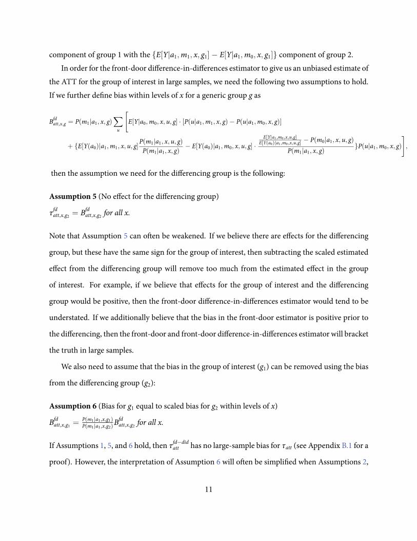
component of group 1 with the {E[Y|a1,m1, x, g1]− E[Y|a1,m0, x, g1]} component of group 2.In order for the front-door difference-in-differences estimator to give us an unbiased estimate of
the ATT for the group of interest in large samples, we need the following two assumptions to hold.If we further de ne bias within levels of x for a generic group g as
Bfdatt,x,g = P(m1|a1, x, g)
∑u
[E[Y|a0,m0, x, u, g] · [P(u|a1,m1, x, g)− P(u|a1,m0, x, g)]
+ {E[Y(a0)|a1,m1, x, u, g]P(m1|a1, x, u, g)P(m1|a1, x, g)
− E[Y(a0)|a1,m0, x, u, g] ·E[Y|a1,m0,x,u,g]
E[Y(a0)|a1,m0,x,u,g] − P(m0|a1, x, u, g)P(m1|a1, x, g)
}P(u|a1,m0, x, g)
],
then the assumption we need for the differencing group is the following:
Assumption 5 (No effect for the differencing group)
τfdatt,x,g2 = Bfdatt,x,g2 for all x.
Note that Assumption 5 can oen be weakened. If we believe there are effects for the differencing
group, but these have the same sign for the group of interest, then subtracting the scaled estimated
effect from the differencing group will remove too much from the estimated effect in the group
of interest. For example, if we believe that effects for the group of interest and the differencing
group would be positive, then the front-door difference-in-differences estimator would tend to be
understated. If we additionally believe that the bias in the front-door estimator is positive prior to
the differencing, then the front-door and front-door difference-in-differences estimator will bracket
the truth in large samples.
We also need to assume that the bias in the group of interest (g1) can be removed using the bias
from the differencing group (g2):
Assumption 6 (Bias for g1 equal to scaled bias for g2 within levels of x)
Bfdatt,x,g1 =
P(m1|a1,x,g1)P(m1|a1,x,g2)B
fdatt,x,g2 for all x.
If Assumptions 1, 5, and 6 hold, then τfd−didatt has no large-sample bias for τatt (see Appendix B.1 for a
proof). However, the interpretation of Assumption 6 will oen be simpli ed when Assumptions 2,
11
3, or 4 hold. is will be discussed in the context of the applications, but one special case is useful
to consider for illustrative purposes. When Assumptions 1 through 5 hold, then Assumption 6 is
equivalent to the following:
{E[Y(a0)|a1,m1, x, g1]− E[Y(a0)|a1,m0, x, g1]} = {E[Y(a0)|a1,m1, x, g2]− E[Y(a0)|a1,m0, x, g2]}
Note that this equality is analogous to the parallel trends assumption for standard difference-in-
differences estimators.
4 Illustrative Application: National JTPA Study
We now illustrate how front-door and front-door difference-in-differences estimates for the aver-
age treatment effect on the treated (ATT) can bracket the experimental truth in the context of the
National JTPA Study, a job training evaluation with both experimental data and a nonexperimental
comparison group. is section builds upon Glynn and Kashin (2013), which demonstrates the
superior performance of front-door adjustment compared to standard covariate adjustments like
regression and matching when estimating the ATT for nonrandomized program evaluations with
one-sided noncompliance. Speci cally for the National JTPA Study, matching adjustments using
the nonexperimental comparison group can come close to the experimental estimates only when
one has “detailed retrospective questions on labor force participation, job spells, earnings” (Heck-
man et al., 1998). However, in the absence of detailed labor force histories, Glynn andKashin (2013)
show that it is possible to create a comparison group that more closely resembles an experimental
control group using the front-door approach. Nonetheless, while the front-door approach is prefer-
able to standard covariate adjustments for the National JTPA Study, the front-door estimates exhibit
positive bias. We thus attempt to address this bias using the front-door-difference-in-differences ap-
proach developed in this paper.
12
In order to implement the difference-in-differences approach, we focus on currently or once
married adult men as the group of interest (henceforth referred to as simply married men). We
measure program impact as the ATT on 18-month earnings in the post-randomization or post-
eligibility period. For married males, the experimental benchmark is $703.27 . Since front-door
adjustment requires compliance information, we cannot use the typical over time difference-in-
differences approach to remove possible bias. However, the focus on married men enables us to
use single adult men as the differencing group in a front-door difference-in-difference approach.
Ideally, we would select a differencing group where Assumption 5 holds; that is, a group where the
treatment would have no effect. In many circumstances, though, it may not be possible to nd a
differencing group where treatment will have no effect. We were unable to nd such a group for the
JTPA Study, and indeed it is likely that Assumption 5 is violated for our differencing group because
the job training program should have effects for singlemen. However, we anticipate the effects of the
training program will be positive, yet smaller, for single men than for married men due to evidence
that marriage improves men’s productivity (e.g., see Korenman and Neumark (1991)). In this case,
the front-door difference-in-differences approach should provide a lower bound on the job training
effect for married men.
e Department of Labor implemented the National JTPA Study between November 1987 and
September 1989 in order to gauge the efficacy of the Job Training Parternship Act (JTPA) of 1982.
e Study randomized JTPA applicants into treatment and control groups at 16 study sites (referred
to as service delivery areas, or SDAs) across the United States. Participants randomized into the
treatment group were allowed to receive JTPA services, whereas those in the control group were
prevented from receiving program services for an 18-month period following random assignment
Age for adult men ranges from 22 to 54 at random assignment / eligibility screening. Once
married men comprises individuals who report that they are widowed, divorced, or separated.
See discussion of how we created our sample and the earnings data in Appendix C.
13
(Bloom et al., 1993; Orr et al., 1994). Crucially for our analysis, 61.4% of married men allowed
to receive JTPA services actually utilized at least one of those services. Moreover, the Study also
collected a nonexperimental comparison group of individuals who met JTPA eligibility criteria but
chose not to apply to the program in the rst place.⁴ Since this sample of eligible nonparticipants
(ENPs) was limited to 4 service delivery areas, we restrict our entire analysis to only these 4 sites.
4.1 Results
e front-door and front-door difference-in-differences estimates for the effect of the JTPAprogram
on married males - our group of interest - are presented in Figure 1 across a range of covariate sets.
Additionally, we present the standard covariate adjusted estimates for comparison. We use OLS
separately within experimental treated and observational control groups (the ENPs) for the stan-
dard estimates. For front-door estimates, we use OLS separately within the “experimental treated
and received treatment” and “experimental treated and didn’t receive treatment” groups. erefore,
these estimates assume linearity and additivity within these comparison groups when conditioning
on covariates, albeit we note that we obtain similar results when usingmore exiblemethods that re-
lax these parametric assumptions. e experimental benchmark (dashed line), is the only estimate
that uses the experimental control units.
First, the front-door estimates exhibit uniformly less estimation error than estimates from stan-
dard covariate adjustment across all conditioning sets in Figure 1. e error in the standard esti-
mates for the null conditioning set and conditioning sets that are combinations of age, race, and
site are negative. e error becomes becomes positive when we include baseline earnings in the
conditioning set. In sharp contrast, the stability of front-door estimates is remarkable. We thus
nd that front-door estimates are preferable to standard covariate adjustment when more detailed
⁴See Appendix C for additional information regarding the ENP sample. See Smith (1994) for
details of ENP screening process.
14
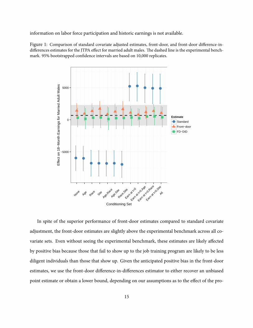
information on labor force participation and historic earnings is not available.
Figure 1: Comparison of standard covariate adjusted estimates, front-door, and front-door difference-in-differences estimates for the JTPA effect for married adult males. e dashed line is the experimental bench-mark. 95% bootstrapped con dence intervals are based on 10,000 replicates.
● ●
● ● ● ● ●
● ●● ● ●
−5000
0
5000
None
AgeRac
eSite
Age,R
ace
Age,S
ite
Race,
Site
Earn
at t=
0
Earn
at t=
0,Age
Earn
at t=
0,Rac
e
Earn
at t=
0,Site
All
Conditioning Set
Effe
ct o
n 18
−M
onth
Ear
ning
s fo
r M
arrie
d A
dult
Mal
es
Estimate
● Standard
Front−door
FD−DID
In spite of the superior performance of front-door estimates compared to standard covariate
adjustment, the front-door estimates are slightly above the experimental benchmark across all co-
variate sets. Even without seeing the experimental benchmark, these estimates are likely affected
by positive bias because those that fail to show up to the job training program are likely to be less
diligent individuals than those that show up. Given the anticipated positive bias in the front-door
estimates, we use the front-door difference-in-differences estimator to either recover an unbiased
point estimate or obtain a lower bound, depending on our assumptions as to the effect of the pro-
15
gram in the differencing group. If we believe that the JTPA program had no effect for single males
(i.e., Assumption 5 holds), andwe also believe thatAssumptions 1 and 6 hold, then the difference-in-
differences estimator will return an unbiased estimate of the effect for the group of interest in large
samples. If, on the other hand, we believe theremight be a non-negative effect for single males, then
we would obtain a lower bound for the effect for the group of interest. In this application, it is more
likely that there was positive effect of the JTPA program for single males, albeit one smaller than for
married males. Hence, the front-door difference-in-differences estimator will likely give us a lower
bound for the effect of the JTPA program formarriedmales. In fact, inmany applications wemay be
unable to nd a differencing group with no effect, yet still be able to use front-door and front-door
difference-in-differences approaches to bound the causal effect of interest given our beliefs about
the sign and relative scale of effects in the group of interest and the differencing group.
When examining the empty conditioning set, the front-door estimate that we obtain for sin-
gle males is $946.09. In order to construct the front-door difference-in-differences estimator, we
have to scale this estimate by the ratio of compliance for married males to compliance for single
males, which is equal to 0.614/0.524 ≈ 1.172. Subtracting the scaled front-door estimate for sin-
gle males from the front-door estimate for married males as shown in (5), we obtain an estimate
of $315.41. is is slightly below the experimental benchmark and thus indeed functions as lower
bound. In sharp contrast to the front-door and front-door difference-in-differences estimates that
rather tightly bound the truth, the bias in the standard estimate is -$6661.90. It is noteworthy that
the front-door estimate acts as an upper bound and the front-door difference-in-differences esti-
mate acts as a lower bound across all conditioning sets presented in Figure 1.
5 Illustrative Application: Early Voting
In this section, we present front-door difference-in-differences estimates for the average treatment
effect on the treated (ATT) of an early in-person voting program in Florida. We want to evaluate
16
the impact that the presence of early voting had upon turnout for some groups in the 2008 and 2012
presidential elections in Florida. In traditional regression or matching approaches (either cross sec-
tional or difference-in-differences), data from Florida would be compared to data from states that
did not implement early in-person voting. ese approaches are potentially problematic because
there may be unmeasured differences between the states, and these differences may change across
elections. One observable manifestation of this is that the candidates on the ballot will be differ-
ent for different states in the same election year and for different election years in the same state.
e front-door and front-door difference-in-differences approaches allows us to solve this problem
by con ning analysis to comparisons made amongst modes of voting within a single presidential
election in Florida.
Additionally, by restricting our analysis to Florida, we are able to use individual-level data from
the Florida Voter Registration Statewide database, maintained since January 2006 by the Florida
Department of State’s Division of Elections. is allows us to avoid the use of self-reported turnout,
provides a very large sample size, and makes it possible to implement all of the estimators discussed
in earlier sections because we observe the mode of voting for each individual. e data contains
two types of records by county: registration records of voters contained within voter extract les
and voter history records contained in voter history les. e former contains demographic infor-
mation - including, crucially for this paper, race - while the latter details the voting mode used by
voters in a given election. e two records can be merged using a unique voter ID available in both
le types. However, voter extract les are snapshots of voter registration records, meaning that a
given voter extract le will not contain all individuals appearing in corresponding voter history le
because individuals move in and out of the voter registration database. We therefore use voter reg-
istration les from four time periods to match our elections of interest: 2006, 2008, and 2010 book
closing records, and the 2012 post-election registration record. Our total population, based on the
total unique voter IDs that appear in any of the voter registration les, is 16.4 million individuals.
Appendix D provides additional information regarding the pre-processing of the Florida data.
17
Information on mode of voting in the voter history les allows us to de ne compliance with the
program for the front-door estimator (i.e., those that utilize EIP voting in the election for which we
are calculating the effect are de ned as compliers). Additionally, we use information on previous
mode of voting to partition the population into a group of interest and differencing groups. In order
tomaximize data reliability, we de ne our group of interest as individuals that used EIP in a previous
election (e.g., 2008 EIP voters are the group of interest when analyzing the turnout effect for the 2012
election). In other words, we are assessing what would have happened to these 2008 EIP voters in
2012 if the EIP program had not been available in 2012. To calculate the EIP effect on turnout for
the 2012 election, we separately consider 2008 and 2010 EIP voters as our groups of interest. For
the 2008 EIP effect on turnout, we rely upon 2006 EIP voters as our group of interest. An attempt to
de ne the group of interest more broadly (e.g., including non-voters) or in terms of earlier elections
(e.g., the 2004 election) would involve the use of less reliable data, and would therefore introduce
methodological complications that are not pertinent to the illustration presented here.⁵ erefore,
the estimates presented in this application are con ned only to those individuals that utilized EIP
in a previous election and hence we cannot comment on the overall turnout effect.
⁵Following Gronke and Stewart (2013), we restrict our analysis to data starting in 2006 due to its
greater reliability than data from 2004. We also might like to extend the group of interest to those
that did not vote in a previous election, but we avoid assessing either 2008 or 2012 EIP effects for
these voters because it is difficult to calculate the eligible electorate and consequently the population
of non-voters. In their analysis of the prevalence of early voting, Gronke and Stewart (2013) use all
voters registered for at least one general election between 2006 and 2012, inclusive, as the total
eligible voter pool. However, using registration records as a proxy for the eligible electorate may be
problematic (McDonald and Popkin, 2001). By focusing on the 2008 voting behavior of individuals
who voted early in 2006, we avoid the need to de ne the eligible electorate and the population of
non-voters.
18
We consider two differencing groups for each analysis: those who voted absentee and those that
voted on election day in a previous election. When considering the 2012 EIP effect for 2008 EIP
voters, for example, we use 2008 absentee and election day voters as our differencing groups. It is
likely that the 2012 EIP program had little or no effect for 2008 absentee voters and perhaps only a
minimal effect for 2008 election day voters, as these groups had already demonstrated an ability to
vote by othermeans. erefore, any apparent effects estimated for these groupswill be primarily due
to bias, and this bias can then be removed from the estimates for the group of interest. As discussed
in earlier sections, the estimates from the differencing groups must be scaled according to the level
of compliance for the group of interest. Finally, the existence of two differencing groups allows us to
conduct a placebo test by using election day voters as the group of interest and the absentee voters
as the differencing group in each case. is analysis is explored below.
Despite the limited scope of the estimates presented here, these results have some bearing on the
recent debates regarding the effects of early voting on turnout. ere have been a number of papers
using cross state comparisons that nd null results for the effects of early voting on turnout (Gronke,
Galanes-Rosenbaum and Miller, 2007; Gronke et al., 2008; Fitzgerald, 2005; Primo, Jacobmeier and
Milyo, 2007; Wol nger, Highton and Mullin, 2005), and Burden et al. (2014) nds a surprising
negative effect of early voting on turnout in 2008.⁶ However, identi cation of turnout effects from
observational data using traditional statistical approaches such as regression or matching rely on
the absence of unobserved confounders that affect both election laws and turnout (Hanmer, 2009).
If these unobserved confounders vary across elections, then traditional difference-in-differences
estimators will also be biased. See Keele and Minozzi (2013) for a discussion within the context
of election laws and turnout. Additionally, a reduction in Florida’s early voting program between
2008 and 2012 provided evidence that early votingmay encourage voter turnout (Herron and Smith,
⁶Burden et al. (2014) examine a broader de nition of early voting that includes no excuse absentee
voting.
19
2014).
e front-door estimators presented here provide an alternative approach to estimating turnout
effects with useful properties. First, front-door adjustment can identify the effect of EIP on turnout
in spite of the endogeneity of election laws that can lead to bias when using standard approaches.
Second, unlike traditional regression, matching, or difference-in-differences based estimates, the
front-door estimators considered here only require data from Florida within a given year. is
means that we can effectively include a Florida/year xed effect in the analysis, and we do not have
to worry about cross-state or cross-time differences skewing turnout numbers across elections. We
also include county xed effects in the analysis in order to control for within-Florida differences.
However, in addition to the limited scope of our analysis, it is important to note that the exclu-
sion restriction is likely violated for this application. Since early in-person voting decreases waiting
times on election day, it is possible that it actually increases turnout among those that only consider
voting on election day. is would mean that front-door estimates would understate the effect if all
other assumptions held because the front-door estimator would be ignoring a positive component
of the effect. Alternatively, Burden et al. (2014) suggest that campaign mobilization for election day
may be inhibited, such that early voting hurts election day turnout. iswouldmean that front-door
estimates would overstate the effect because the front-door estimator would be ignoring a negative
component of the effect. is can also be seen by examining the bias formula (4) (because the EIP
treatment is assigned at the state level, Assumptions 1 and 4 will hold).
Taken together, the overall effect of these exclusion restrictions is unclear and would depend
on the strength of the two violations. e predictions also become less clear once we consider the
front-door difference-in-differences approach, where additional bias in front-door estimates might
cancelwith bias in the estimates for the differencing group. For the remainder of this analysis, wewill
assume that all such violations of the exclusion restriction cancel out in the front-door difference-
in-differences estimator. is is implicit in Assumption 6.
20
5.1 Results
In order to construct the front-door estimate of the 2008 EIP effect for our group of interest, we
calculate the turnout rate in 2008 for all individuals who voted early in 2006. We also calculate the
non-complier turnout rate in 2008 by excluding all individuals who voted early in 2008 from the
previous calculation. e front-door estimate of the 2008 EIP effect for 2006 early voters is thus the
difference between the former and latter turnout rates. Quite intuitively, the counterfactual turnout
rate without EIP for the group of interest is the observed turnout rate of non-compliers in that
group. We do not devote much attention to the front-door estimates seeing as they are implausibly
large.⁷ e positive bias stems from the fact that 2006 EIP voters would be more likely to vote in
2008, even in the absence of EIP, than the 2006 non-EIP group (this group includes individuals
that did not vote in 2006). In terms of the bias formula in (4), this is equivalent to saying that
E[Y(a0)|a1,m1, x] > E[Y(a0)|a1,m0, x].
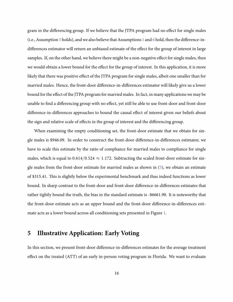
In order to address this bias, we present front-door difference-in-differences estimates for the
2008 EIP program in Figure 2. e estimates all utilize county xed effects and are calculated sepa-
rately across the racial categories.⁸ e front-door difference-in-differences estimates for the group
of interest (2006 EIP voters) are in green, with 2008 absentee voters (triangles) and 2008 election
day voters (squares) as the differencing groups. e former, for example, is constructed as the dif-
ference between front-door estimates for 2006 early voters and the front-door estimates for 2006
⁷Front-door estimates are available in Appendix E.
⁸We calculate the FD-DID estimates within each county and then average using the population
of the group of interest as the county weight. Due to very small sample sizes in a few counties, we
are occasionally unable to calculate front-door estimates. In these cases, we omit the counties from
the weighted average when calculating the front-door estimates with xed effects. We note that due
to their small size, these counties are unlikely to exert any signi cant impact upon the estimates
regardless.
21
absentee voters, with the front-door estimates for the differencing group scaled by the ratio of early
voter compliance to absentee voter compliance as shown in (5). e purple estimates in Figure 2
represent the placebo test, with 2006 election day voters standing in as the group of interest and
the absentee voters as the differencing group. In general, we note that if there exists more than one
plausible differencing group, then one should conduct the analysis using each differencing group
separately, as well as a placebo test to verify the plausibility of Assumption 5.
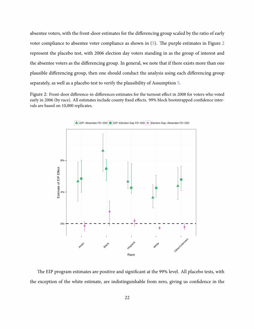
Figure 2: Front-door difference-in-differences estimates for the turnout effect in 2008 for voters who votedearly in 2006 (by race). All estimates include county xed effects. 99% block bootstrapped con dence inter-vals are based on 10,000 replicates.
0%
4%
8%
Asian
Black
Hispan
ic
Whit
e
Other
/Unk
nown
Race
Est
imat
e of
EIP
Effe
ct
EIP−Absentee FD−DID EIP−Election Day FD−DID Election Day−Absentee FD−DID
e EIP program estimates are positive and signi cant at the 99% level. All placebo tests, with
the exception of the white estimate, are indistinguishable from zero, giving us con dence in the
22
estimated EIP effects. Even if the slightly negative placebo estimate for whites indicates a true neg-
ative effect of the 2008 EIP program, and not bias, the weighted average of the green and the purple
effects (i.e., the 2008 EIP effect for the 2006 EIP and election day voters together), again produces a
slightly positive estimate. erefore, we generally nd evidence that early voting increased turnout
for the subset of individuals who voted early in 2006. Moreover, comparing the point estimates
across races, we nd some evidence that the program had a disproportionate bene t for African-
Americans.
Our methodology uses voting behavior in 2006 only to de ne groups and does not compare
turnout of voters across elections. us any differences between presidential election and midterm
election voters (see e.g. Gronke and Toffey (2008)) does not pose a prima facie problem for the
analysis. Moreover, using early voters in a midterm election as the group of interest for calculating
the EIP effect in a presidential election does not require additional assumptions beyond what one
would need if using early voters in a presidential election. Nonetheless, a potential downside of the
preceeding results is that the estimated 2008 EIP is limited to those individuals who voted early in
the 2006 midterm election, whereas we might want to extend the group of interest to early voters
in a presidential election. Unfortunately, we cannot present the estimates with the group of interest
and the differencing groups de ned in terms of 2004 behavior because the data from 2004 are not
reliable (as mentioned above). As a robustness check, we also estimate the effect of the early voting
program in the 2012 election, for which we can de ne the group of interest and the differencing
groups using 2008 voting behavior. However, as discussed above, Florida’s early voting program
was reduced between 2008 and 2012, so we should not expect the results to be equivalent.
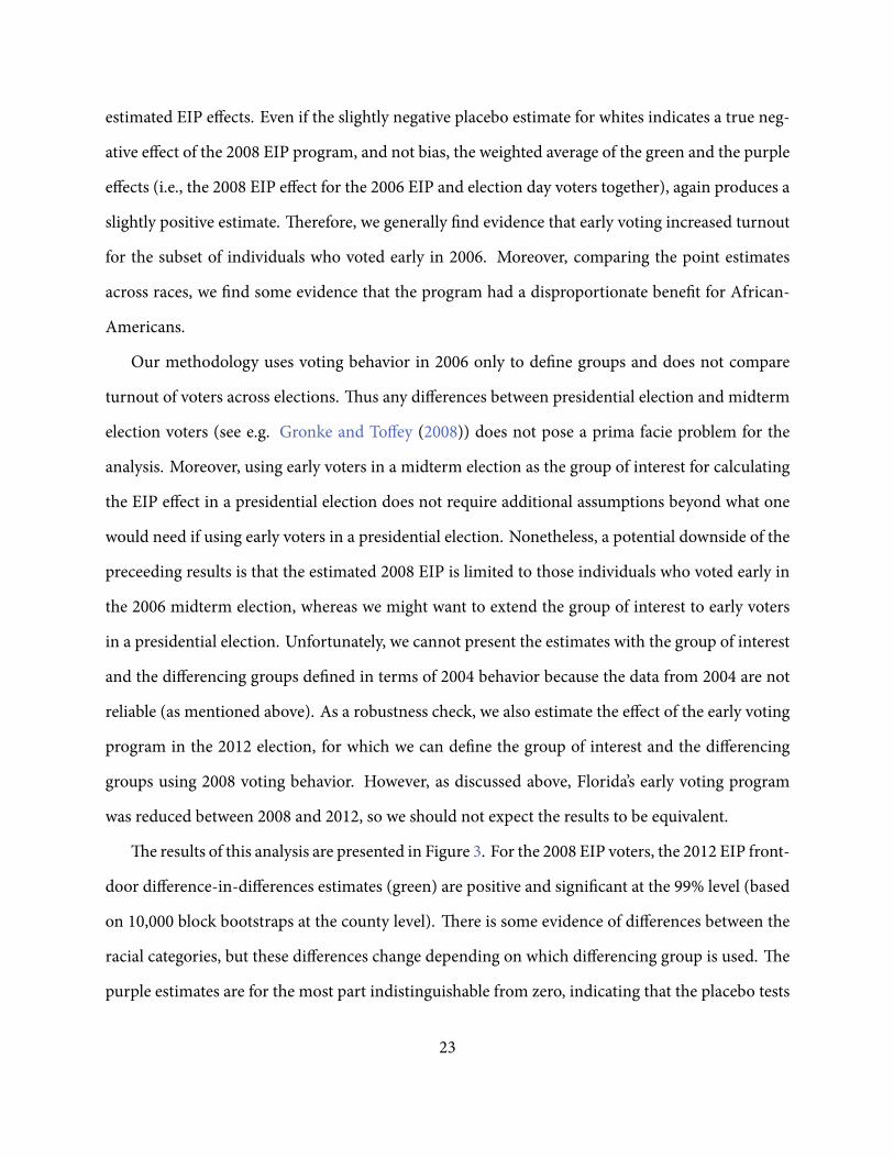
e results of this analysis are presented in Figure 3. For the 2008 EIP voters, the 2012 EIP front-
door difference-in-differences estimates (green) are positive and signi cant at the 99% level (based
on 10,000 block bootstraps at the county level). ere is some evidence of differences between the
racial categories, but these differences change depending on which differencing group is used. e
purple estimates are for the most part indistinguishable from zero, indicating that the placebo tests
23
have mostly been passed. e slightly negative purple estimate for whites again indicates either
bias, or perhaps a negative effect of the 2012 EIP program for white 2008 election day voters. Note
that even if we believe this estimate, the weighted average of the green and the purple effects for
whites (i.e., the 2012 EIP effect for the 2008 EIP and election day voters together) produces a slightly
positive estimate, albeit this estimate is indistinguishable from zero. In sum, the evidence points to
a slightly positive turnout effect of the 2012 EIP program on the 2008 EIP users.
Figure 3: Front-door difference-in-differences estimates for the turnout effect in 2012 for voters who votedearly in 2008 (by race). All estimates include county xed effects. 99% block bootstrapped con dence inter-vals are based on 10,000 replicates.
0%
1%
2%
3%
Asian
Black
Hispan
ic
Whit
e
Other
/Unk
nown
Race
Est
imat
e of
EIP
Effe
ct
EIP−Absentee FD−DID EIP−Election Day FD−DID Election Day−Absentee FD−DID
It is also notable that the size of the estimated EIP effect for 2012 is less than half the estimated
EIP effect for 2008 when looking at EIP voters as the group of interest across all races. ere are two
24
potential reasons for this. First, our estimates for the 2008 EIP program are obtained using groups
de ned by 2006midterm election behavior and as alreadymentioned, midterm election early voters
are likely different than presidential election early voters. Second, the nature of the early voting
program changed between the 2008 and 2012 elections, notably removing the option of voting early
on the Sunday prior to the election and all-together near-halving of the early voting period from 14
days to 8 days (Gronke and Stewart, 2013; Herron and Smith, 2014). is change might possibly
reduce the effect of the EIP program in 2012 when compared to 2008 - a nding consistent with the
conclusion made by Herron and Smith (2014) that individuals who voted in 2008 on the Sunday
prior to the election were disproportionately less likely to vote in 2012.
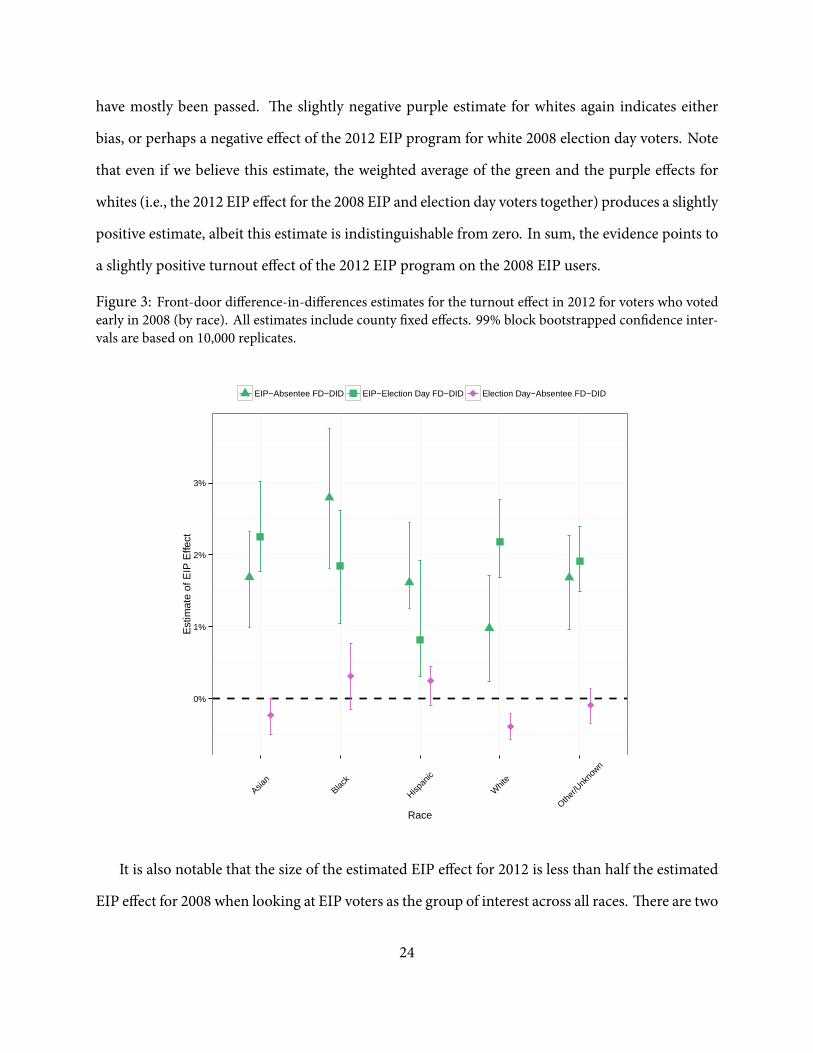
In order to isolate the consequences of the change in the early voting program from changes in
the construction of the group of interest and differencing groups, we re-estimate the effects of the
2012 EIP program using 2010 EIP voters as the group of interest (green), and using 2010 absentee
(triangles) and election day voters (squares) as the differencing groups. Placebo tests are reported
using 2010 election day voters as the group of interest and 2010 absentee voters as the differencing
group (purple). ese results are presented in Figure 4, and they are quite similar to the results in
Figure 2. is provides some evidence that if we were able to obtain reliable data from the 2004
election, our estimates for the 2008 EIP program would likely have produced something similar to
Figure 3 when using 2004 EIP voters as the group of interest, and 2004 absentee (triangles) and
election day voters (squares) as the differencing groups. However, the estimates in Figure 2 are
slightly larger than estimates in Figure 4. is is consistent with the reduction in the early voting
window for the 2012 election.
6 Conclusion
In this paper, we have developed front-door difference-in-differences estimators for nonrandom-
ized program evaluations with one-sided noncompliance and an exclusion restriction. ese esti-
25
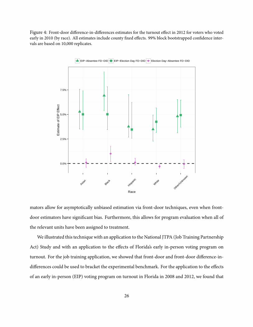
Figure 4: Front-door difference-in-differences estimates for the turnout effect in 2012 for voters who votedearly in 2010 (by race). All estimates include county xed effects. 99% block bootstrapped con dence inter-vals are based on 10,000 replicates.
0.0%
2.5%
5.0%
7.5%
Asian
Black
Hispan
ic
Whit
e
Other
/Unk
nown
Race
Est
imat
e of
EIP
Effe
ctEIP−Absentee FD−DID EIP−Election Day FD−DID Election Day−Absentee FD−DID
mators allow for asymptotically unbiased estimation via front-door techniques, even when front-
door estimators have signi cant bias. Furthermore, this allows for program evaluation when all of
the relevant units have been assigned to treatment.
We illustrated this technique with an application to theNational JTPA (Job Training Partnership
Act) Study and with an application to the effects of Florida’s early in-person voting program on
turnout. For the job training application, we showed that front-door and front-door difference-in-
differences could be used to bracket the experimental benchmark. For the application to the effects
of an early in-person (EIP) voting program on turnout in Florida in 2008 and 2012, we found that
26
for two separate differencing groups, the program had small but signi cant positive effects. While
the scope of the analysis is limited, this result provides some evidence to counter previous results in
the literature that early voting programs had either no effect or negative effects.
Finally, the results in this paper have implications for research design and analysis. First, the
examples demonstrate the importance of collecting post-treatment variables that represent compli-
ancewith, or uptake of, the treatment. Such information allows front-door and front-door difference-
in-differences analyses to be carried out as a robustness check on standard approaches. Second,
the bracketing of the experimental benchmark in the JTPA application show that control units are
not always necessary for credible causal inference. is is a remarkable nding that should make a
number of previously infeasible studies possible (e.g., when it is unethical or impossible to withhold
treatment from individuals).
27
References
Bloom, Howard S., Larry L. Orr, George Cave, Stephen Bell and Fred Doolittle. 1993. “e National
JTPA Study: Title IIA Impacts on Earnings and Employment at 18 Months.” Bethesda, MD: . 14
Brady, Henry E., David Collier and Jason Seawright. 2006. “Toward a Pluralistic Vision of Method-
ology.” Political Analysis 14:353–368. 2
Burden, Barry C., David T. Canon, Kenneth R. Mayer and Donald P. Moynihan. 2014. “Election
Laws, Mobilization, and Turnout: e Unanticipated Consequences of Election Reform.” Amer-
ican Journal of Political Science 58(1):95–109. 19, 20
Collier, David andHenry E. Brady. 2004. Rethinking Social Inquiry: Diverse Tools, Shared Standards.
Lanham, MD: Rowman & Little eld. 2
Cox, David R. and Nanny Wermuth. 1995. “Discussion of ‘Causal diagrams for empirical research’.”
Biometrika 82:688–689. 2
Fitzgerald, Mary. 2005. “Greater Convenience but not Greater Turnout: e Impact of Alterna-
tive Voting Methods on Electoral Participation in the United States.” American Politics Research
33:842–867. 19
George, A.L. and A. Bennett. 2005. Case studies and theory development in the social sciences. Mit
Press. 2
Glynn, Adam andKevinQuinn. 2011. “WhyProcessMatters for Causal Inference.”Political Analysis
19(3):273–286. 2
Glynn, Adam and Konstantin Kashin. 2013. “Front-door Versus Back-door Adjustment with Un-
measuredConfounding: Bias Formulas for Front-door andHybridAdjustments.”Working Paper.
2, 12
28
Gronke, Paul and Charles Stewart. 2013. “Early Voting in Florida.” Paper presented at the Annual
Meeting of the Midwest Political Science Association, Chicago, IL. 18, 25, 38
Gronke, Paul and Daniel Krantz Toffey. 2008. “e Psychological and Institutional Determinants
of Early Voting.” Journal of Social Issues 64(3):503–524. 23
Gronke, Paul, Eva Galanes-Rosenbaum, Peter A. Miller and Daniel Toffey. 2008. “Convenience
Voting.” Annual Review of Political Science 11:437–455. 19
Gronke, Paul, Eva Galanes-Rosenbaum and Peter Miller. 2007. “Early Voting and Turnout.” PS:
Political Science and Politics XL. 19
Hanmer, Michael J. 2009. Discount Voting: Voter Registration Reforms andeir Effects. Cambridge
University Press. 19
Heckman, James, Hidehiko Ichimura, Jeffrey Smith and Petra Todd. 1998. “Characterizing selection
bias using experimental data.” Econometrica 66:1017–1098. 12, 37
Heckman, James J., Robert J. LaLonde and Jeffrey A. Smith. 1999. e Economics and Econometrics
ofActive LaborMarket Programs. InHandbook of Labor Economics, Volume III, ed.O.Ashenfelter
and D. Card. Elsevier Science North-Holland. 6
Herron, Michael C. and Daniel A. Smith. 2014. “Race, Party, and the Consequences of Restricting
Early Voting in Florida in the 2012 General Election.” Political Research Quarterly . 19, 25
Imbens, Guido and Donald Rubin. 1995. “Discussion of ‘Causal diagrams for empirical research’.”
Biometrika 82:694–695. 2
Joffe, Marshall M. 2001. “Using information on realized effects to determine prospective causal
effects.” Journal of the Royal Statistical Society. Series B, Statistical Methodology pp. 759–774. 2
29

Kaufman, Sol, Jay S. Kaufman and Richard F. MacLehose. 2009. “Analytic bounds on causal risk
differences in directed acyclic graphs with three observed binary variables.” Journal of Statistical
Planning and Inference 139:3473–87. 2
Keele, Luke and William Minozzi. 2013. “How Much Is Minnesota Like Wisconsin? Assumptions
and Counterfactuals in Causal Inference with Observational Data.” Political Analysis 21(2):193–
216. 19
King, Gary, RobertO. Keohane and SidneyVerba. 1994. Designing Social Inquiry: Scienti c Inference
in Qualitative Research. 1 ed. Princeton University Press. 2
Korenman, Sanders and David Neumark. 1991. “Does Marriage Really Make Men More Produc-
tive?” e Journal of Human Resources 26(2):282–307. 13
Kuroki, Manabu and Masami Miyakawa. 1999. “Identi ability Criteria for Causal Effects of Joint
Interventions.” J. Japan Statist. Soc. 29(2):105–117. 2
McDonald, Michael P. and Samuel L. Popkin. 2001. “e Myth of the Vanishing Voter.” American
Political Science Review 95:963–974. 18
Orr, Larry L., Howard S. Bloom, Stephen H. Bell, Winston Lin, George Cave and Fred Doolittle.
1994. “e National JTPA Study: Impacts, Bene ts, And Costs of Title IIA.” Bethesda, MD: . 14
Pearl, Judea. 1995. “Causal diagrams for empirical research.” Biometrika 82:669–710. 2, 6
Primo, David M., Matthew L. Jacobmeier and Jeffrey Milyo. 2007. “Estimating the Impact of State
Policies and Institutions with Mixed-Level Data.” State Politics & Policy Quarterly 7:446–459. 19
Shpitser, Ilya and Judea Pearl. 2006. “Identi cation of Conditional Interventional Distributions.”
Proceedings of the Twenty Second Conference on Uncertainty in Arti cial Intelligence (UAI). 2
Smith, Jeffrey A. 1994. “Sampling Frame for the Eligible Non-Participant Sample.” Mimeo . 14
30
Stewart, Charles. 2012. “Declaration of Dr. Charles Stewart III.” State of Florida vs. United States of
America. 38
Tian, Jin and Judea Pearl. 2002a. A general identi cation condition for causal effects. In Proceedings
of the National Conference on Arti cial Intelligence. Menlo Park, CA; Cambridge, MA; London;
AAAI Press; MIT Press; 1999 pp. 567–573. 2
Tian, Jin and Judea Pearl. 2002b. On the identi cation of causal effects. In Proceedings of the Amer-
ican Association of Arti cial Intelligence. 2
VanderWeele, Tyler J. 2009. “On the relative nature of overadjustment and unnecessary adjustment.”
Epidemiology 20(4):496–499. 2
Wol nger, Raymond E., Benjamin Highton and Megan Mullin. 2005. “How Postregistration Laws
Affect the Turnout of Citizens Registered to Vote.” State Politics & Policy Quarterly 5:1–23. 19
31
A ATT Proofs
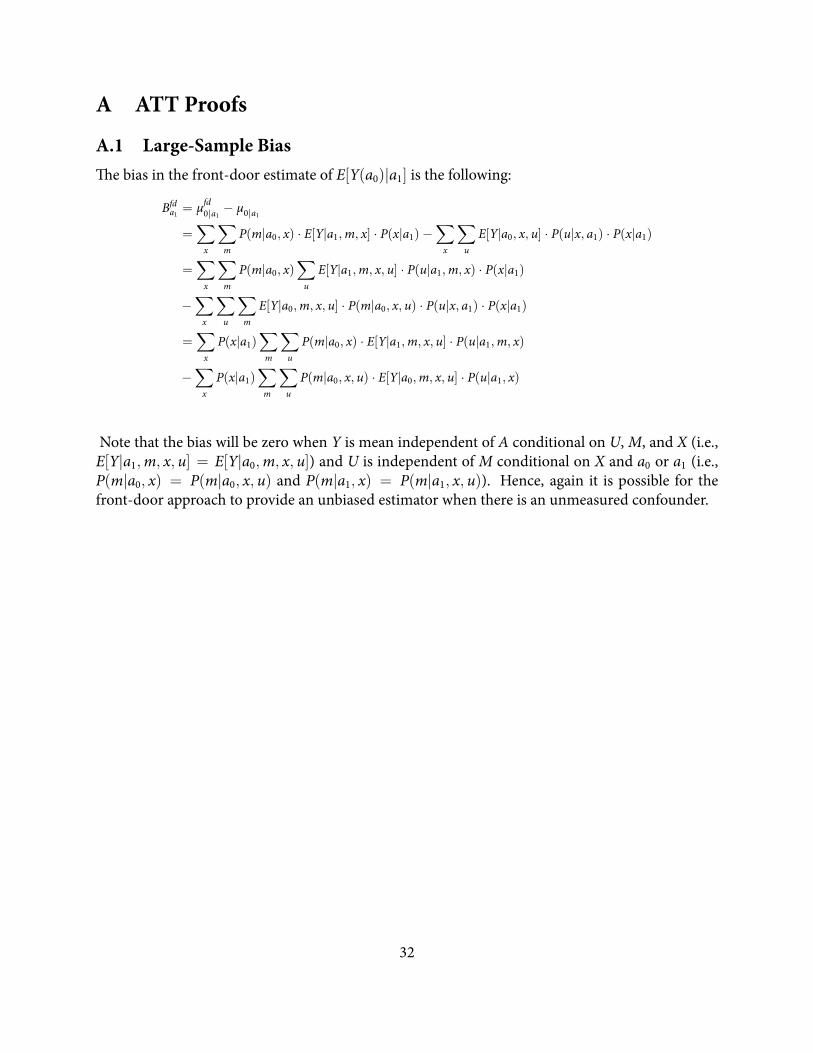
A.1 Large-Sample Biase bias in the front-door estimate of E[Y(a0)|a1] is the following:
Bfda1= μfd0|a1
− μ0|a1
=∑x
∑m
P(m|a0, x) · E[Y|a1,m, x] · P(x|a1)−∑x
∑u
E[Y|a0, x, u] · P(u|x, a1) · P(x|a1)
=∑x
∑m
P(m|a0, x)∑u
E[Y|a1,m, x, u] · P(u|a1,m, x) · P(x|a1)
−∑x
∑u
∑m
E[Y|a0,m, x, u] · P(m|a0, x, u) · P(u|x, a1) · P(x|a1)
=∑x
P(x|a1)∑m
∑u
P(m|a0, x) · E[Y|a1,m, x, u] · P(u|a1,m, x)
−∑x
P(x|a1)∑m
∑u
P(m|a0, x, u) · E[Y|a0,m, x, u] · P(u|a1, x)
Note that the bias will be zero when Y is mean independent of A conditional on U, M, and X (i.e.,E[Y|a1,m, x, u] = E[Y|a0,m, x, u]) and U is independent of M conditional on X and a0 or a1 (i.e.,P(m|a0, x) = P(m|a0, x, u) and P(m|a1, x) = P(m|a1, x, u)). Hence, again it is possible for thefront-door approach to provide an unbiased estimator when there is an unmeasured confounder.
32
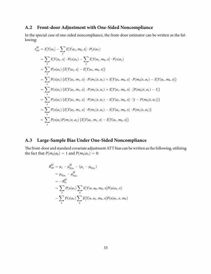
A.2 Front-door Adjustment with One-Sided NoncomplianceIn the special case of one-sided noncompliance, the front-door estimator can be written as the fol-lowing:
τfdatt = E[Y|a1]−∑x
E[Y|a1,m0, x] · P(x|a1)
=∑x
E[Y|a1, x] · P(x|a1)−∑x
E[Y|a1,m0, x] · P(x|a1)
=∑x
P(x|a1) {E[Y|a1, x]− E[Y|a1,m0, x]}
=∑x
P(x|a1) {E[Y|a1,m1, x] · P(m1|x, a1) + E[Y|a1,m0, x] · P(m0|x, a1)− E[Y|a1,m0, x]}
=∑x
P(x|a1) {E[Y|a1,m1, x] · P(m1|x, a1) + E[Y|a1,m0, x] · [P(m0|x, a1)− 1]}
=∑x
P(x|a1) {E[Y|a1,m1, x] · P(m1|x, a1)− E[Y|a1,m0, x] · [1 − P(m0|x, a1)]}
=∑x
P(x|a1) {E[Y|a1,m1, x] · P(m1|x, a1)− E[Y|a1,m0, x] · P(m1|x, a1)}
=∑x
P(x|a1)P(m1|x, a1) {E[Y|a1,m1, x]− E[Y|a1,m0, x]}
A.3 Large-Sample Bias Under One-Sided Noncompliancee front-door and standard covariate adjustmentATTbias can bewritten as the following, utilizingthe fact that P(m0|a0) = 1 and P(m0|a1) = 0:
Bfdatt = μ1 − μfd0|a1− (μ1 − μ0|a1
)
= μ0|a1− μfd0|a1
= −Bfda1
=∑x
P(x|a1)∑u
E[Y|u, a0,m0, x]P(u|a1, x)
−∑x
P(x|a1)∑u
E[Y|u, a1,m0, x]P(u|a1, x,m0)
33
Adding and subtracting∑
x P(x)∑
u E[Y|a0,m0, u] · P(u|a1,m0):
=∑x
P(x|a1)∑u
E[Y|u, a0,m0, x] · [P(u|a1, x)− P(u|a1, x,m0)]
−∑x
P(x|a1)∑u{E[Y|u, a1,m0, x]− E[Y|u, a0,m0, x]} · P(u|a1,m0, x)
Bstdatt = μ1 − μstd0|a1− (μ1 − μ0|a1
)
= μ0|a1− μstd0|a1
= −Bstda1
=∑x
P(x|a1)∑u
E[Y|u, a0,m0, x] · [P(u|a1, x)− P(u|a0, x)]
A.4 Front-door Bias Simpli catione front-door bias under one-sided noncompliance can be written as:
Bfdatt =∑x
P(x|a1)∑u
E[Y|a0,m0, x, u][P(u|a1, x)− P(u|a1,m0, x)︸ ︷︷ ︸ε
] (7)
+∑x
P(x|a1)∑u{E[Y|a0,m0, x, u]− E[Y|a1,m0, x, u]︸ ︷︷ ︸
η
}P(u|a1,m0, x). (8)
ε can be rewritten as:
ε = P(u|a1, x)− P(u|a1,m0, x)= P(u|a1,m1, x)P(m1|a1, x) + P(u|a1,m0, x)P(m0|a1, x)− P(u|a1,m0, x)= P(u|a1,m1, x)P(m1|a1, x) + P(u|a1,m0, x)[P(m0|a1, x)− 1]= P(u|a1,m1, x)P(m1|a1, x)− P(u|a1,m0, x)P(m1|a1, x)= P(m1|a1, x)[P(u|a1,m1, x)− P(u|a1,m0, x)].
34

We can also expand η as:
η = E[Y|a0,m0, x, u]− E[Y|a1,m0, x, u]= E[Y|a0, x, u]− E[Y|a1,m0, x, u]= E[Y(a0)|a0, x, u]− E[Y|a1,m0, x, u]= E[Y(a0)|a1, x, u]− E[Y|a1,m0, x, u]= E[Y(a0)|a1,m1, x, u]P(m1|a1, x, u) + E[Y(a0)|a1,m0, x, u]P(m0|a1, x, u)− E[Y|a1,m0, x, u]
= E[Y(a0)|a1,m1, x, u]P(m1|a1, x, u)− E[Y(a0)|a1,m0, x, u] · {E[Y|a1,m0, x, u]
E[Y(a0)|a1,m0, x, u]− P(m0|a1, x, u)}
= P(m1|a1, x)
E[Y(a0)|a1,m1, x, u]P(m1|a1, x, u)P(m1|a1, x)
− E[Y(a0)|a1,m0, x, u] ·E[Y|a1,m0,x,u]
E[Y(a0)|a1,m0,x,u] − P(m0|a1, x, u)P(m1|a1, x)
.
We note that the bias can be written as scaled by the compliance proportion within levels of x(P(m1|a1, x)).
We can thus rewrite front-door bias under one-sided noncompliance as:
Bfdatt =
∑x
P(x|a1)P(m1|a1, x)∑u
[E[Y|a0,m0, x, u] · [P(u|a1,m1, x)− P(u|a1,m0, x)]
+
E[Y(a0)|a1,m1, x, u]P(m1|a1, x, u)P(m1|a1, x)
− E[Y(a0)|a1,m0, x, u] ·E[Y|a1,m0,x,u]
E[Y(a0)|a1,m0,x,u] − P(m0|a1, x, u)P(m1|a1, x)
P(u|a1,m0, x)
].
A.5 Front-door Bias Under Assumption 3Assumption 3 and binary M implies that ε = 0:
P(m1|a1, x, u) =P(u|a1,m1, x) · P(m1|a1, x)
P(u|a1, x)
1 =P(u|a1,m1, x)P(u|a1, x)
P(u|a1, x) = P(u|a1,m1, x)
Since M is binary, by similar logic as above we know that P(u|a1, x) = P(u|a1,m0, x).
35
erefore:
ε = P(m1|a1, x)[P(u|a1,m1, x)− P(u|a1,m0, x)]= P(m1|a1, x)[P(u|a1, x)− P(u|a1, x)]= 0
Under Assumption 3, we can simplify front-door bias to:
Bfdatt =∑x
P(x|a1)P(m1|a1, x)∑u
[E[Y(a0)|a1,m1, x, u]
P(m1|a1, x, u)P(m1|a1, x)
− E[Y(a0)|a1,m0, x, u] ·E[Y|a1,m0,x,u]
E[Y(a0)|a1,m0,x,u] − P(m0|a1, x, u)P(m1|a1, x)
]· P(u|a1, x).
B Front-Door Difference-in-Differences Proofs
B.1 No Large-Sample Bias in the Front-door Difference-in-Differences Esti-mator
First de ne τatt,x = E[Y(a1)|a1, x] − E[Y(a0)|a1, x]. It is well known that τatt =∑
x τatt,xP(x|a1).erefore in order to show that τfd−did
att has no bias, we need only show a lack of bias for τatt,x withinlevels of x. If Assumptions 5 and 6 hold, then the front-door difference-in-differences estimator hasno large-sample bias:
τfd−didatt,x = τfdatt,x,g1 −
P(m1|a1, x, g1)P(m1|a1, x, g2)
τfdatt,x,g2
= τatt,x + Bfdatt,x,g1 −
P(m1|a1, x, g1)P(m1|a1, x, g2)
τfdatt,x,g2
= τatt,x + Bfdatt,x,g1 −
P(m1|a1, x, g1)P(m1|a1, x, g2)
Bfdatt,x,g2
= τatt,x + Bfdatt,x,g1 − Bfd
att,x,g1
= τatt,x
C National JTPA Study DataOur paper uses the following samples from the National JTPA Study: experimental active treatmentgroup, experimental control group, and the nonexperimental / eligible nonparticipant (ENP) group.For our purposes, the active treatment groupmeans receving any JTPA service, although the type of
36
services actually received varied across individuals.⁹ In this analysis, we only examine adult malesand follow the sample restrictions in Appendix B1 of Heckman et al. (1998). We also restrict ourattention to the 4 service delivery areas at which the ENP sample was collected: Fort Wayne, IN;Corpus Christi, TX; Jackson, MS, and Providence, RI. e nal sample sizes (by marital status) arepresented in Table 1.
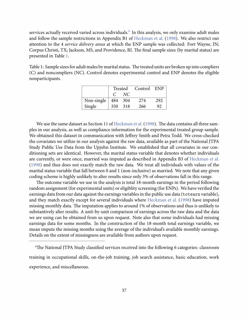
Table 1: Sample sizes for adultmales bymarital status. e treated units are brokenup into compliers(C) and noncompliers (NC). Control denotes experimental control and ENP denotes the eligiblenonparticipants.
Treated Control ENPC NC
Non-single 484 304 274 292Single 350 318 266 92
We use the same dataset as Section 11 of Heckman et al. (1998). e data contains all three sam-ples in our analysis, as well as compliance information for the experimental treated group sample.We obtained this dataset in communication with Jeffrey Smith and Petra Todd. We cross-checkedthe covariates we utilize in our analysis against the raw data, available as part of the National JTPAStudy Public Use Data from the Upjohn Institute. We established that all covariates in our con-ditioning sets are identical. However, the marital status variable that denotes whether individualsare currently, or were once, married was imputed as described in Appendix B3 of Heckman et al.(1998) and thus does not exactly match the raw data. We treat all individuals with values of themarital status variable that fall between 0 and 1 (non-inclusive) as married. We note that any givencoding scheme is highly unlikely to alter results since only 3% of observations fall in this range.
e outcome variable we use in the analysis is total 18-month earnings in the period followingrandom assignment (for experimental units) or eligiblity screening (for ENPs). We have veri ed theearnings data from our data against the earnings variables in the public use data (totearn variable),and they match exactly except for several individuals where Heckman et al. (1998) have imputedmissing monthly data. e imputation applies to around 1% of observations and thus is unlikely tosubstantively alter results. A unit-by-unit comparison of earnings across the raw data and the datawe are using can be obtained from us upon request. Note also that some individuals had missingearnings data for some months. In the construction of the 18-month total earnings variable, wemean impute the missing months using the average of the individual’s available monthly earnings.Details on the extent of missingness are available from authors upon request.
⁹e National JTPA Study classi ed services received into the following 6 categories: classroom
training in occupational skills, on-the-job training, job search assistance, basic education, work
experience, and miscellaneous.
37
D Florida Voting DataTo construct our population of eligible voters, we examine individuals that have appeared in one offour voter registration snapshots: book closing records from10/10/2006, 10/20/2008, and 10/18/2010,as well as a 2012 election recap record from 1/4/2013. is yields a total population of 16,371,725individuals that we are able to subset by race (Asian / Paci c Islander, Black (not Hispanic), His-panic, White (Not Hispanic), and Other). Note that the Other category contains individuals whoself-identify as American Indian / Alaskan Native, Multiracial, or Other, as well as individuals forwhom race is unknown. In cases where race changes across voter registration snapshots for the samevoter, we use the latest available self-reported race. Such changes affect only 1.1% of observations.e breakdown of the the population by race is presented in the rightmost column of Table 2.
We use voter history les from 08/03/2013 to subset the population by voting mode in eachelection. e voter history les required pre-processing before we could use them for estimation.As mentioned in Gronke and Stewart (2013) and Stewart (2012), there is an issue of duplicationof voter identi cation numbers within the same election. In some cases, this duplication is ratherinnocuous because the voting mode is identical across records. In these cases, we simply removeduplicate records and include the voter in our analysis. In other cases, voters are recorded as bothhaving voted in a given election and not having voted (code “N”). In these cases, we assume thatthe voter did indeed cast a ballot and use that code. Finally, there are a few instances in which avoter is recorded to have voted in multiple ways. For example, a voter history le may indicatethat a voter voted both absentee and early at a given election. While Gronke and Stewart (2013)indicates that voters may legitimately appear multiple times in the voter history le, this makes thetask of stratifying by voting mode difficult. As a result, we choose to exclude individuals who arerecorded to have voted using more than one mode. When analyzing the 2008 election subsettingby 2006 voting modes, we exclude 385 individuals. e corresponding numbers for analysis of the2012 election subsetting using 2008 and 2010 voting groups are 1951 and 2998, respectively. esegures are dwarfed by the sample sizes and thereby highly unlikely to exert any serious effect upon
our estimates.We also made several choices regarding the de nition of voting modes. Speci cally, we classi-
ed anyone who voted absentee (code “A”) and whose absentee ballot was not counted (code “B”)as having voted absentee. We classi ed anyone who voted early (code “E”) and anyone cast a pro-visional ballot early (code “F”) as having voted early. Finally, we classify anyone who voted at thepolls (code “Y”) and cast a provisional ballot at the polls (code “Z”) as having voted on election day.We do not use the code “P”, which indicates that an individual cast a provisional ballot that was notcounted since we cannot ascertain whether it was cast on election day, early, or as an absentee voter.
Another difficulty with the data is de ning the eligible electorate and thus individuals who didnot vote. While the voter history les have a code “N” for did not vote, most individuals who do notvote are not present in the voter history les at all. For example, for the 2008 election there were no“N” codes at all in the voter history les. erefore, we count an individual as not having voted in agiven election if they appeared in the voter registration les at one point but are either not presentin the voter history le for that election or are coded as “N”.
38
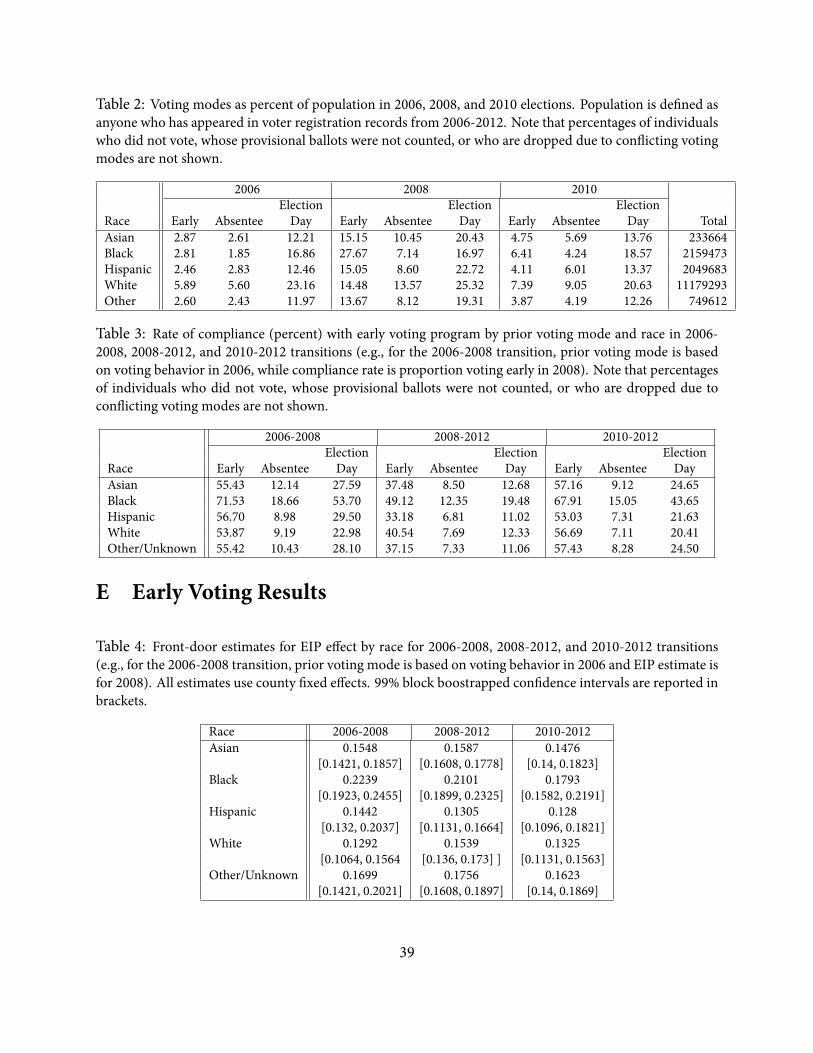
Table 2: Voting modes as percent of population in 2006, 2008, and 2010 elections. Population is de ned asanyone who has appeared in voter registration records from 2006-2012. Note that percentages of individualswho did not vote, whose provisional ballots were not counted, or who are dropped due to con icting votingmodes are not shown.
2006 2008 2010Election Election Election
Race Early Absentee Day Early Absentee Day Early Absentee Day TotalAsian 2.87 2.61 12.21 15.15 10.45 20.43 4.75 5.69 13.76 233664Black 2.81 1.85 16.86 27.67 7.14 16.97 6.41 4.24 18.57 2159473Hispanic 2.46 2.83 12.46 15.05 8.60 22.72 4.11 6.01 13.37 2049683White 5.89 5.60 23.16 14.48 13.57 25.32 7.39 9.05 20.63 11179293Other 2.60 2.43 11.97 13.67 8.12 19.31 3.87 4.19 12.26 749612
Table 3: Rate of compliance (percent) with early voting program by prior voting mode and race in 2006-2008, 2008-2012, and 2010-2012 transitions (e.g., for the 2006-2008 transition, prior voting mode is basedon voting behavior in 2006, while compliance rate is proportion voting early in 2008). Note that percentagesof individuals who did not vote, whose provisional ballots were not counted, or who are dropped due tocon icting voting modes are not shown.
2006-2008 2008-2012 2010-2012Election Election Election
Race Early Absentee Day Early Absentee Day Early Absentee DayAsian 55.43 12.14 27.59 37.48 8.50 12.68 57.16 9.12 24.65Black 71.53 18.66 53.70 49.12 12.35 19.48 67.91 15.05 43.65Hispanic 56.70 8.98 29.50 33.18 6.81 11.02 53.03 7.31 21.63White 53.87 9.19 22.98 40.54 7.69 12.33 56.69 7.11 20.41Other/Unknown 55.42 10.43 28.10 37.15 7.33 11.06 57.43 8.28 24.50
E Early Voting Results
Table 4: Front-door estimates for EIP effect by race for 2006-2008, 2008-2012, and 2010-2012 transitions(e.g., for the 2006-2008 transition, prior voting mode is based on voting behavior in 2006 and EIP estimate isfor 2008). All estimates use county xed effects. 99% block boostrapped con dence intervals are reported inbrackets.
Race 2006-2008 2008-2012 2010-2012Asian 0.1548 0.1587 0.1476
[0.1421, 0.1857] [0.1608, 0.1778] [0.14, 0.1823]Black 0.2239 0.2101 0.1793
[0.1923, 0.2455] [0.1899, 0.2325] [0.1582, 0.2191]Hispanic 0.1442 0.1305 0.128
[0.132, 0.2037] [0.1131, 0.1664] [0.1096, 0.1821]White 0.1292 0.1539 0.1325
[0.1064, 0.1564 [0.136, 0.173] ] [0.1131, 0.1563]Other/Unknown 0.1699 0.1756 0.1623
[0.1421, 0.2021] [0.1608, 0.1897] [0.14, 0.1869]
39
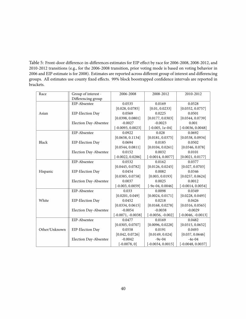
Table 5: Front-door difference-in-differences estimates for EIP effect by race for 2006-2008, 2008-2012, and2010-2012 transitions (e.g., for the 2006-2008 transition, prior voting mode is based on voting behavior in2006 and EIP estimate is for 2008). Estimates are reported across different group of interest and differencinggroups. All estimates use county xed effects. 99% block boostrapped con dence intervals are reported inbrackets.
Race Group of interest - 2006-2008 2008-2012 2010-2012Differencing groupEIP-Absentee 0.0535 0.0169 0.0528
[0.028, 0.0785] [0.01, 0.0233] [0.0352, 0.0757]Asian EIP-Election Day 0.0569 0.0225 0.0501
[0.0398, 0.0801] [0.0177, 0.0303] [0.0344, 0.0739]Election Day-Absentee -0.0027 -0.0023 0.001
[-0.0093, 0.0023] [-0.005, 1e-04] [-0.0036, 0.0048]EIP-Absentee 0.0922 0.028 0.0692
[0.0658, 0.1134] [0.0181, 0.0375] [0.0538, 0.0934]Black EIP-Election Day 0.0694 0.0185 0.0502
[0.0544, 0.0811] [0.0104, 0.0261] [0.0346, 0.078]Election Day-Absentee 0.0152 0.0032 0.0101
[-0.0022, 0.0286] [-0.0014, 0.0077] [0.0021, 0.0177]EIP-Absentee 0.0532 0.0162 0.0377
[0.0445, 0.0782] [0.0126, 0.0245] [0.027, 0.0703]Hispanic EIP-Election Day 0.0454 0.0082 0.0346
[0.0385, 0.0758] [0.003, 0.0193] [0.0257, 0.0624]Election Day-Absentee 0.0037 0.0025 0.0012
[-0.003, 0.0059] [-9e-04, 0.0046] [-0.0014, 0.0054]EIP-Absentee 0.033 0.0098 0.0349
[0.0201, 0.049] [0.0024, 0.0171] [0.0228, 0.0495]White EIP-Election Day 0.0452 0.0218 0.0426
[0.0334, 0.0615] [0.0168, 0.0278] [0.0316, 0.0565]Election Day-Absentee -0.0054 -0.0038 -0.0029
[-0.0071, -0.0038] [-0.0056, -0.002] [-0.0046, -0.0013]EIP-Absentee 0.0477 0.0169 0.0482
[0.0305, 0.0707] [0.0096, 0.0228] [0.0315, 0.0652]Other/Unknown EIP-Election Day 0.0558 0.0191 0.0493
[0.042, 0.0726] [0.0149, 0.024] [0.037, 0.0646]Election Day-Absentee -0.0042 -9e-04 -4e-04
[-0.0078, 0] [-0.0034, 0.0015] [-0.0048, 0.0037]
40