1

Structured Compressed Sensing:From Theory to Applications

Marco F. Duarte Member, IEEE, and Yonina C. Eldar, Senior Member, IEEE

Abstract

Compressed sensing (CS) is an emerging field that has attracted considerable research interest over the past fewyears. Previous review articles in CS limit their scope to standard discrete-to-discrete measurement architecturesusing matrices of randomized nature and signal models based on standard sparsity. In recent years, CS has workedits way into several new application areas. This, in turn, necessitates a fresh look on many of the basics of CS. Therandom matrix measurement operator must be replaced by more structured sensing architectures that correspond tothe characteristics of feasible acquisition hardware. The standard sparsity prior has to be extended to include a muchricher class of signals and to encode broader data models, including continuous-time signals. In our overview, thetheme is exploiting signal and measurement structure in compressive sensing. The prime focus is bridging theoryand practice; that is, to pinpoint the potential of structured CS strategies to emerge from the math to the hardware.Our summary highlights new directions as well as relations to more traditional CS, with the hope of serving bothas a review to practitioners wanting to join this emerging field, and as a reference for researchers that attempts toput some of the existing ideas in perspective of practical applications.

I. INTRODUCTION AND MOTIVATION

Compressed sensing (CS) is an emerging field that has attracted considerable research interest in the signalprocessing community. Since its introduction only several years ago [1, 2], thousands of papers have appearedin this area, and hundreds of conferences, workshops, and special sessions have been dedicated to this growingresearch field.

Due to the vast interest in this topic, there exist several excellent review articles on the basics of CS [3–5]. Thesearticles focused on the first CS efforts: the use of standard discrete-to-discrete measurement architectures usingmatrices of randomized nature, where no structure beyond sparsity is assumed on the signal or in its representation.This basic formulation already required the use of sophisticated mathematical tools and rich theory in order to

Manuscript submitted September 1, 2010; revised February 18, 2011 and June 21, 2011; accepted July 3, 2011.Copyright (c) 2011 IEEE. Personal use of this material is permitted. However, permission to use this material for any other purposes

must be obtained from the IEEE by sending a request to pubs-permissions@ieee.org.MFD was supported in part by NSF Supplemental Funding DMS-0439872 to UCLA-IPAM, P.I. R. Caflisch. YCE was supported in part

by the Israel Science Foundation under Grant no. 170/10, and by a Magneton grant from the Israel Ministry of Industry and Trade.MFD is with the Department of Electrical and Computer Engineering, University of Massachusetts, Amherst, MA 01003. Email:

mduarte@ecs.umass.eduYCE is with the Department of Electrical Engineering, Technion—Israel Institute of Technology, Haifa 32000, Israel. She is also a

Visiting Professor at Stanford University, Stanford, CA, USA. E-mail: yonina@ee.technion.ac.il

arX

iv:1

106.

6224

v2 [

cs.I

T]

28

Jul 2

011

2

analyze recovery approaches and provide performance guarantees. It was therefore essential to confine attentionto this simplified setting in the early stages of development of the CS framework.

Essentially all analog-to-digital converters (ADCs) to date follow the celebrated Shannon-Nyquist theorem whichrequires the sampling rate to be at least twice the bandwidth of the signal. This basic principle underlies themajority of digital signal processing (DSP) applications such as audio, video, radio receivers, radar applications,medical devices and more. The ever growing demand for data, as well as advances in radio frequency (RF)technology, have promoted the use of high-bandwidth signals, for which the rates dictated by the Shannon-Nyquist theorem impose severe challenges both on the acquisition hardware and on the subsequent storage andDSP processors. CS was motivated in part by the desire to sample wideband signals at rates far lower thanthe Shannon-Nyquist rate, while still maintaining the essential information encoded in the underlying signal. Inpractice, however, much of the work to date on CS has focused on acquiring finite-dimensional sparse vectorsusing random measurements. This precludes the important case of continuous-time (i.e., analog) input signals, aswell as practical hardware architectures which inevitably are structured. Achieving the holy grail of compressiveADCs and increased resolution requires a broader framework which can treat more general signal models, includingcontinuous-time signals with various types of structure, as well as practical measurement schemes.

In recent years, the area of CS has branched out to many new fronts and has worked its way into severalapplication areas. This, in turn, necessitates a fresh look on many of the basics of CS. The random matrix mea-surement operator, fundamental in all early presentations of CS, must be replaced by more structured measurementoperators that correspond to the application of interest, such as wireless channels, analog sampling hardware, sensornetworks and optical imaging. The standard sparsity prior that has characterized early work in CS has to be extendedto include a much richer class of signals: signals that have underlying low-dimensional structure, not necessarilyrepresented by standard sparsity, and signals that can have arbitrary dimensions, not only finite-dimensional vectors.

A significant part of the recent work on CS from the signal processing community can be classified into twomajor contribution areas. The first group consists of theory and applications related to CS matrices that are notcompletely random and that often exhibit considerable structure. This largely follows from efforts to model theway the samples are acquired in practice, which leads to sensing matrices that inherent their structure from the realworld. The second group includes signal representations that exhibit structure beyond sparsity and broader classesof signals, such as continuous-time signals with infinite-dimensional representations. For many types of signals,such structure allows for a higher degree of signal compression when leveraged on top of sparsity. Additionally,infinite-dimensional signal representations provide an important example of richer structure which clearly cannotbe described using standard sparsity. Since reducing the sampling rate in analog signals was one of the drivingforces behind CS, building a theory that can accommodate low-dimensional signals in arbitrary Hilbert spaces isclearly an essential part of the CS framework. Both of these categories are motivated by real-world CS involvingactual hardware implementations.

In our review, the theme is exploiting signal and measurement structure in CS. The prime focus is bridgingtheory and practice – that is, to pinpoint the potential of CS strategies to emerge from the math to the hardwareby generalizing the underlying theory where needed. We believe that this is an essential ingredient in taking CSto the next step: incorporating this fast growing field into real-world applications. Considerable efforts have beendevoted in recent years by many researchers to adapt the theory of CS to better solve real-world signal acquisition

3

challenges. This has also led to parallel low-rate sampling schemes that combine the principles of CS with therich theory of sampling such as the finite rate of innovation (FRI) [6–8] and Xampling frameworks [9, 10]. Thereare already dozens of papers dealing with these broad ideas. In this review we have strived to provide a coherentsummary, highlighting new directions and relations to more traditional CS. This material can both serve as a reviewto those wanting to join this emerging field, as well as a reference that attempts to summarize some of the existingresults in the framework of practical applications. Our hope is that this presentation will attract the interest of bothmathematicians and engineers in the desire to promote the CS premise into practical applications, and encouragefurther research into this new frontier.

This review paper is organized as follows. Section II provides background motivating the formulation of CS andthe layout of the review. A primer on standard CS theory is presented in Section III. This material serves as a basisfor the later developments. Section IV reviews alternative constructions for structured CS matrices beyond thosegenerated completely at random. In Section V we introduce finite-dimensional signal models that exhibit additionalsignal structure. This leads to the more general union-of-subspaces framework, which will play an important rolein the context of structured infinite-dimensional representations as well. Section VI extends the concepts of CS toinfinite-dimensional signal models and introduces recent compressive ADCs which have been developed based onthe Xampling and FRI frameworks. For each of the matrices and models introduced, we summarize the details ofthe theoretical and algorithmic frameworks and provide example applications where the structure is applicable.

II. BACKGROUND

We live in a digital world. Telecommunication, entertainment, medical devices, gadgets, business – all revolvearound digital media. Miniature sophisticated black-boxes process streams of bits accurately at high speeds.Nowadays, electronic consumers feel natural that a media player shows their favorite movie, or that their surroundsystem synthesizes pure acoustics, as if sitting in the orchestra instead of the living room. The digital world playsa fundamental role in our everyday routine, to such a point that we almost forget that we cannot “hear” or “watch”these streams of bits, running behind the scenes.

Analog to digital conversion lies at the heart of this revolution. ADC devices translate the physical informationinto a stream of numbers, enabling digital processing by sophisticated software algorithms. The ADC task isinherently intricate: its hardware must hold a snapshot of a fast-varying input signal steady while acquiringmeasurements. Since these measurements are spaced in time, the values between consecutive snapshots are lost. Ingeneral, therefore, there is no way to recover the analog signal unless some prior on its structure is incorporated.

After sampling, the numbers or bits retained must be stored and later processed. This requires ample storagedevices and sufficient processing power. As technology advances, so does the requirement for ever-increasingamounts of data, imposing unprecedented strains on both the ADC devices and the subsequent DSP and storagemedia. How then does consumer electronics keep up with these high demands? Fortunately, most of the data weacquire can be discarded without much perceptual loss. This is evident in essentially all compression techniquesused to date. However, this paradigm of high-rate sampling followed by compression does not alleviate the largestrains on the acquisition device and on the DSP. In his seminal work on CS [1], Donoho posed the ultimate goalof merging compression and sampling: “why go to so much effort to acquire all the data when most of what weget will be thrown away? Can’t we just directly measure the part that won’t end up being thrown away?”.

4

A. Shannon-Nyquist Theorem

ADCs provide the interface between an analog signal being recorded and a suitable discrete representation. Acommon approach in engineering is to assume that the signal is bandlimited, meaning that the spectral contentsare confined to a maximal frequency B. Bandlimited signals have limited time variation, and can therefore beperfectly reconstructed from equispaced samples with rate at least 2B, termed the Nyquist rate. This fundamentalresult is often attributed in the engineering community to Shannon-Nyquist [11, 12], although it dates back toearlier works by Whittaker [13] and Kotelnikov [14].Theorem 1. [12] If a function x(t) contains no frequencies higher than B hertz, then it is completely determinedby giving its ordinates at a series of points spaced 1/(2B) seconds apart.

A fundamental reason for processing at the Nyquist rate is the clear relation between the spectrum of x(t) andthat of its samples x(nT ), so that digital operations can be easily substituted for their analog counterparts. Digitalfiltering is an example where this relation is successfully exploited. Since the power spectral densities of analogand discrete random processes are associated in a similar manner, estimation and detection of parameters of analogsignals can be performed by DSP. In contrast, compression is carried out by a series of algorithmic steps, which,in general, exhibit a nonlinear complicated relationship between the samples x(nT ) and the stored data.

While this framework has driven the development of signal acquisition devices for the last half century, theincreasing complexity of emerging applications dictates increasingly higher sampling rates that cannot always bemet using available hardware. Advances in related fields such as wideband communication and RF technologyopen a considerable gap with ADC devices. Conversion speeds which are twice the signal’s maximal frequencycomponent have become more and more difficult to obtain. Consequently, alternatives to high rate sampling aredrawing considerable attention in both academia and industry.

Structured analog signals can often be processed far more efficiently than what is dictated by the Shannon-Nyquist theorem, which does not take any structure into account. For example, many wideband communicationsignals are comprised of several narrow transmissions modulated at high carrier frequencies. A common practice inengineering is demodulation in which the input signal is multiplied by the carrier frequency of a band of interest,in order to shift the contents of the narrowband transmission from the high frequencies to the origin. Then,commercial ADC devices at low rates are utilized. Demodulation, however, requires knowing the exact carrierfrequency. In this review we focus on structured models in which the exact parameters defining the structure areunknown. In the context of multiband communications, for example, the carrier frequencies may not be known, ormay be changing over time. The goal then is to build a compressed sampler which does not depend on the carrierfrequencies, but can nonetheless acquire and process such signals at rates below Nyquist.

B. Compressed Sensing and Beyond

A holy grail of CS is to build acquisition devices that exploit signal structure in order to reduce the samplingrate, and subsequent demands on storage and DSP. In such an approach, the actual information contents dictatethe sampling rate, rather than the dimensions of the ambient space in which the signal resides. The challenges inachieving this task both theoretically and in terms of hardware design can be reduced substantially when consideringfinite-dimensional problems in which the signal to be measured can be represented as a discrete finite-length vector.

5

This has spurred a surge of research on various mathematical and algorithmic aspects of sensing sparse signals,which were mainly studied for discrete finite vectors.

At its core, CS is a mathematical framework that studies accurate recovery of a signal represented by a vectorof length N from M N measurements, effectively performing compression during signal acquisition. Themeasurement paradigm consists of linear projections, or inner products, of the signal vector into a set of carefullychosen projection vectors that act as a multitude of probes on the information contained in the signal. In thefirst part of this review (Sections III and IV) we survey the fundamentals of CS and show how the ideas can beextended to allow for more elaborate measurement schemes that incorporate structure into the measurement process.When considering real-world acquisition schemes, the choices of possible measurement matrices are dictated bythe constraints of the application. Thus, we must deviate from the general randomized constructions and applystructure within the projection vectors that can be easily implemented by the acquisition hardware. Section IVfocuses on such alternatives; we survey both existing theory and applications for several classes of structured CSmatrices. In certain applications, there exist hardware designs that measure analog signals at a sub-Nyquist rate,obtaining measurements for finite-dimensional signal representations via such structured CS matrices.

In the second part of this review (Sections V and VI) we expand the theory of CS to signal models tailored toexpress structure beyond standard sparsity. A recent emerging theoretical framework that allows a broader classof signal models to be acquired efficiently is the union of subspaces model [15–20]. We introduce this frameworkand some of its applications in a finite-dimensional context in Section V, which include more general notions ofstructure and sparsity. Combining the principles and insights from the previous sections, in Section VI we extendthe notion of CS to analog signals with infinite-dimensional representations. This new framework, referred to asXampling [9, 10], relies on more general signal models – union of subspaces and FRI signals – together withguidelines on how to exploit these mathematical structures in order to build sensing devices that can directlyacquire analog signals at reduced rates. We then survey several compressive ADCs that result from this broaderframework.

III. COMPRESSED SENSING BASICS

Compressed sensing (CS) [1–5] offers a framework for simultaneous sensing and compression of finite-dimensionalvectors, that relies on linear dimensionality reduction. Specifically, in CS we do not acquire x directly but ratheracquire M < N linear measurements y = Φx using an M ×N CS matrix Φ. We refer to y as the measurementvector. Ideally, the matrix Φ is designed to reduce the number of measurements M as much as possible whileallowing for recovery of a wide class of signals x from their measurement vectors y. However, the fact that M < N

renders the matrix Φ rank-defficient, meaning that it has a nonempty nullspace; this, in turn, implies that for anyparticular signal x0 ∈ RN , an infinite number of signals x will yield the same measurements y0 = Φx0 = Φx forthe chosen CS matrix Φ.

The motivation behind the design of the matrix Φ is, therefore, to allow for distinct signals x, x′ within a classof signals of interest to be uniquely identifiable from their measurements y = Φx, y′ = Φx′, even though M N .We must therefore make a choice on the class of signals that we aim to recover from CS measurements.

6

A. Sparsity

Sparsity is the signal structure behind many compression algorithms that employ transform coding, and is themost prevalent signal structure used in CS. Sparsity also has a rich history of applications in signal process-ing problems in the last century (particularly in imaging), including denoising, deconvolution, restoration, andinpainting [21–23].

To introduce the notion of sparsity, we rely on a signal representation in a given basis ψiNi=1 for RN . Everysignal x ∈ RN is representable in terms of N coefficients θiNi=1 as x =

∑Ni=1 ψiθi; arranging the ψi as columns

into the N ×N matrix Ψ and the coefficients θi into the N × 1 coefficient vector θ, we can write succinctly thatx = Ψθ, with θ ∈ RN . Similarly, if we use a frame1 Ψ containing N unit-norm column vectors of length L withL < N (i.e., Ψ ∈ RL×N ), then for any vector x ∈ RL there exist infinitely many decompositions θ ∈ RN such thatx = Ψθ. In a general setting, we refer to Ψ as the sparsifying dictionary [24]. While our exposition is restrictedto real-valued signals, the concepts are extendable to complex signals as well [25, 26].

We say that a signal x is K-sparse in the basis or frame Ψ if there exists a vector θ ∈ RN with only K N

nonzero entries such that x = Ψθ. We call the set of indices corresponding to the nonzero entries the support ofθ and denote it by supp(θ). We also define the set ΣK that contains all signals x that are K-sparse.

A K-sparse signal can be efficiently compressed by preserving only the values and locations of its nonzerocoefficients, using O(K log2N) bits: coding each of the K nonzero coefficient’s locations takes log2N bits, whilecoding the magnitudes uses a constant amount of bits that depends on the desired precision, and is independentof N . This process is known as transform coding, and relies on the existence of a suitable basis or frame Ψ thatrenders signals of interest sparse or approximately sparse.

For signals that are not exactly sparse, the amount of compression depends on the number of coefficients ofθ that we keep. Consider a signal x whose coefficients θ, when sorted in order of decreasing magnitude, decayaccording to the power law

|θ(I(n))| ≤ S n−1/r, n = 1, . . . , N, (1)

where I indexes the sorted coefficients. Thanks to the rapid decay of their coefficients, such signals are well-approximated by K-sparse signals. The best K-term approximation error for such a signal obeys

σΨ(x,K) := arg minx′∈ΣK

‖x− x′‖2 ≤ CSK−s, (2)

with s = 1r − 1

2 and C denoting a constant that does not depend on N [27]. That is, the signal’s best approximationerror (in an `2-norm sense) has a power-law decay with exponent s as K increases. We dub such a signal s-compressible. When Ψ is an orthonormal basis, the best sparse approximation of x is obtained by hard thresholdingthe signal’s coefficients, so that only the K coefficients with largest magnitudes are preserved. The situation isdecidedly more complicated when Ψ is a general frame, spurring the development of sparse approximation methods,a subject that we will focus on in Section III-C.

When sparsity is used as the signal structure enabling CS, we aim to recover x from y by exploiting its sparsity.In contrast with transform coding, we do not operate on the signal x directly, but rather only have access to the

1A matrix Ψ is said to be a frame if there exist constants A, B such that A‖x‖2 ≤ ‖Ψx‖2 ≤ B‖x‖2 for all x.

7

CS measurement vector y. Our goal is to push M as close as possible to K in order to perform as much signal“compression” during acquisition as possible. In the sequel, we will assume that Ψ is taken to be the identity basisso that the signal x = θ is itself sparse. In certain cases we will explicitly define a different basis or frame Ψ thatarises in a specific application of CS.

B. Design of CS Matrices

The main design criteria for the CS matrix Φ is to enable the unique identification of a signal of interest xfrom its measurements y = Φx. Clearly, when we consider the class of K-sparse signals ΣK , the number ofmeasurements M > K for any matrix design, since the identification problem has K unknowns even when thesupport Ω = supp(x) of the signal x is provided. In this case, we simply restrict the matrix Φ to its columnscorresponding to the indices in Ω, denoted by ΦΩ, and then use the pseudoinverse to recover the nonzero coefficientsof x:

xΩ = Φ†Ωy. (3)

Here xΩ is the restriction of the vector x to the set of indices Ω, and M† = (MTM)−1MT denotes thepseudoinverse of the matrix M. The implicit assumption in (3) is that ΦΩ has full column-rank so that thereis a unique solution to the equation y = ΦΩxΩ.

We begin by determining properties of Φ that guarantee that distinct signals x, x′ ∈ ΣK , x 6= x′, lead to differentmeasurement vectors Φx 6= Φx′. In other words, we want each vector y ∈ RM to be matched to at most onevector x ∈ ΣK such that y = Φx. A key relevant property of the matrix in this context is its spark.Definition 1. [28] The spark spark(Φ) of a given matrix Φ is the smallest number of columns of Φ that arelinearly dependent.

The spark is related to the Kruskal Rank from the tensor product literature; the matrix Φ has Kruskal rankspark(Φ)− 1. This definition allows us to pose the following straightforward guarantee.Theorem 2. [28] If spark(Φ) > 2K, then for each measurement vector y ∈ RM there exists at most one signalx ∈ ΣK such that y = Φx.

It is easy to see that spark(Φ) ∈ [2,M + 1], so that Theorem 2 yields the requirement M ≥ 2K.While Theorem 2 guarantees uniqueness of representation for K-sparse signals, computing the spark of a general

matrix Φ has combinatorial computational complexity, since one must verify that all sets of columns of a certainsize are linearly independent. Thus, it is preferable to use properties of Φ that are easily computable to providerecovery guarantees. The coherence of a matrix is one such property.

Definition 2. [28–31] The coherence µ(Φ) of a matrix Φ is the largest absolute inner product between any twocolumns of Φ:

µ(Φ) = max1≤i 6=j≤N

|〈φi, φj〉|‖φi‖2‖φj‖2

. (4)

It can be shown that µ(Φ) ∈[√

N−MM(N−1) , 1

]; the lower bound is known as the Welch bound [32, 33]. Note

that when N M , the lower bound is approximately µ(Φ) ≥ 1/√M . One can tie the coherence and spark of a

matrix by employing the Gershgorin circle theorem.

8

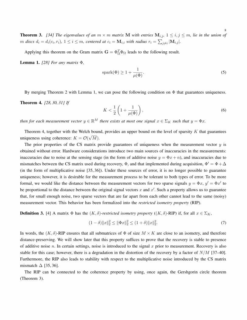
Theorem 3. [34] The eigenvalues of an m ×m matrix M with entries Mi,j , 1 ≤ i, j ≤ m, lie in the union ofm discs di = di(ci, ri), 1 ≤ i ≤ m, centered at ci = Mi,i with radius ri =

∑j 6=i |Mi,j |.

Applying this theorem on the Gram matrix G = ΦTΩΦΩ leads to the following result.

Lemma 1. [28] For any matrix Φ,

spark(Φ) ≥ 1 +1

µ(Φ). (5)

By merging Theorem 2 with Lemma 1, we can pose the following condition on Φ that guarantees uniqueness.

Theorem 4. [28, 30, 31] If

K <1

2

(1 +

1

µ(Φ)

), (6)

then for each measurement vector y ∈ RM there exists at most one signal x ∈ ΣK such that y = Φx.

Theorem 4, together with the Welch bound, provides an upper bound on the level of sparsity K that guaranteesuniqueness using coherence: K = O(

√M).

The prior properties of the CS matrix provide guarantees of uniqueness when the measurement vector y isobtained without error. Hardware considerations introduce two main sources of inaccuracies in the measurements:inaccuracies due to noise at the sensing stage (in the form of additive noise y = Φx+n), and inaccuracies due tomismatches between the CS matrix used during recovery, Φ, and that implemented during acquisition, Φ′ = Φ+∆

(in the form of multiplicative noise [35, 36]). Under these sources of error, it is no longer possible to guaranteeuniqueness; however, it is desirable for the measurement process to be tolerant to both types of error. To be moreformal, we would like the distance between the measurement vectors for two sparse signals y = Φx, y′ = Φx′ tobe proportional to the distance between the original signal vectors x and x′. Such a property allows us to guaranteethat, for small enough noise, two sparse vectors that are far apart from each other cannot lead to the same (noisy)measurement vector. This behavior has been formalized into the restricted isometry property (RIP).

Definition 3. [4] A matrix Φ has the (K, δ)-restricted isometry property ((K, δ)-RIP) if, for all x ∈ ΣK ,

(1− δ)‖x‖22 ≤ ‖Φx‖22 ≤ (1 + δ)‖x‖22. (7)

In words, the (K, δ)-RIP ensures that all submatrices of Φ of size M ×K are close to an isometry, and thereforedistance-preserving. We will show later that this property suffices to prove that the recovery is stable to presenceof additive noise n. In certain settings, noise is introduced to the signal x prior to measurement. Recovery is alsostable for this case; however, there is a degradation in the distortion of the recovery by a factor of N/M [37–40].Furthermore, the RIP also leads to stability with respect to the multiplicative noise introduced by the CS matrixmismatch ∆ [35, 36].

The RIP can be connected to the coherence property by using, once again, the Gershgorin circle theorem(Theorem 3).

9

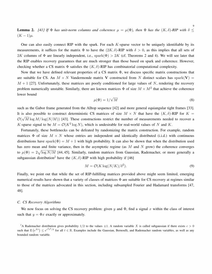
Lemma 2. [41] If Φ has unit-norm columns and coherence µ = µ(Φ), then Φ has the (K, δ)-RIP with δ ≤(K − 1)µ.

One can also easily connect RIP with the spark. For each K-sparse vector to be uniquely identifiable by itsmeasurements, it suffices for the matrix Φ to have the (2K, δ)-RIP with δ > 0, as this implies that all sets of2K columns of Φ are linearly independent, i.e., spark(Φ) > 2K (cf. Theorems 2 and 4). We will see later thatthe RIP enables recovery guarantees that are much stronger than those based on spark and coherence. However,checking whether a CS matrix Φ satisfies the (K, δ)-RIP has combinatorial computational complexity.

Now that we have defined relevant properties of a CS matrix Φ, we discuss specific matrix constructions thatare suitable for CS. An M × N Vandermonde matrix V constructed from N distinct scalars has spark(V) =

M + 1 [27]. Unfortunately, these matrices are poorly conditioned for large values of N , rendering the recoveryproblem numerically unstable. Similarly, there are known matrices Φ of size M ×M2 that achieve the coherencelower bound

µ(Φ) = 1/√M (8)

such as the Gabor frame generated from the Alltop sequence [42] and more general equiangular tight frames [33].It is also possible to construct deterministic CS matrices of size M × N that have the (K, δ)-RIP for K =

O(√M logM/ log(N/M)) [43]. These constructions restrict the number of measurements needed to recover a

K-sparse signal to be M = O(K2 logN), which is undesirable for real-world values of N and K.Fortunately, these bottlenecks can be defeated by randomizing the matrix construction. For example, random

matrices Φ of size M × N whose entries are independent and identically distributed (i.i.d.) with continuousdistributions have spark(Φ) = M + 1 with high probability. It can also be shown that when the distribution usedhas zero mean and finite variance, then in the asymptotic regime (as M and N grow) the coherence convergesto µ(Φ) = 2

√logN/M [44, 45]. Similarly, random matrices from Gaussian, Rademacher, or more generally a

subgaussian distribution2 have the (K, δ)-RIP with high probability if [46]

M = O(K log(N/K)/δ2). (9)

Finally, we point out that while the set of RIP-fulfilling matrices provided above might seem limited, emergingnumerical results have shown that a variety of classes of matrices Φ are suitable for CS recovery at regimes similarto those of the matrices advocated in this section, including subsampled Fourier and Hadamard transforms [47,48].

C. CS Recovery Algorithms

We now focus on solving the CS recovery problem: given y and Φ, find a signal x within the class of interestsuch that y = Φx exactly or approximately.

2A Rademacher distribution gives probability 1/2 to the values ±1. A random variable X is called subgaussian if there exists c > 0

such that E(eXt

)≤ ec

2t2/2 for all t ∈ R. Examples include the Gaussian, Bernoulli, and Rademacher random variables, as well as anybounded random variable.

10

When we consider sparse signals, the CS recovery process consists of a search for the sparsest signal x thatyields the measurements y. By defining the `0 “norm” of a vector ‖x‖0 as the number of nonzero entries in x,the simplest way to pose a recovery algorithm is using the optimization

x = arg minx∈RN

‖x‖0 subject to y = Φx. (10)

Solving (10) relies on an exhaustive search and is successful for all x ∈ ΣK when the matrix Φ has the sparsesolution uniqueness property (i.e., for M as small as 2K, see Theorems 2 and 4). However, this algorithm hascombinatorial computational complexity, since we must check whether the measurement vector y belongs to thespan of each set of K columns of Φ, K = 1, 2, . . . , N . Our goal, therefore, is to find computationally feasiblealgorithms that can successfully recover a sparse vector x from the measurement vector y for the smallest possiblenumber of measurements M .

An alternative to the `0 “norm” used in (10) is to use the `1 norm, defined as ‖x‖1 =∑N

n=1 |x(n)|. The resultingadaptation of (10), known as basis pursuit (BP) [22], is formally defined as

x = arg minx∈RN

‖x‖1 subject to y = Φx. (11)

Since the `1 norm is convex, (11) can be seen as a convex relaxation of (10). Thanks to the convexity, thisalgorithm can be implemented as a linear program, making its computational complexity polynomial in the signallength [49].3

The optimization (11) can be modified to allow for noise in the measurements y = Φx+ n; we simply changethe constraint on the solution to

x = arg minx∈RN

‖x‖1 subject to ‖y − Φx‖2 ≤ ε, (12)

where ε ≥ ‖n‖2 is an appropriately chosen bound on the noise magnitude. This modified optimization is known asbasis pursuit with inequality constraints (BPIC) and is a quadratic program with polynomial complexity solvers [49].The Lagrangian relaxation of this quadratic program is written as

x = arg minx∈RN

‖x‖1 + λ‖y − Φx‖2, (13)

and is known as basis pursuit denoising (BPDN). There exist many efficient solvers to find BP, BPIC, and BPDNsolutions; for an overview, see [51].

Oftentimes, a bounded-norm noise model is overly pessimistic, and it may be reasonable instead to assume thatthe noise is random. For example, additive white Gaussian noise n ∼ N (0, σ2I) is a common choice. Approachesdesigned to address stochastic noise include complexity-based regularizaton [52] and Bayesian estimation [53].These methods pose probabilistic or complexity-based priors, respectively, on the set of observable signals.The particular prior is then leveraged together with the noise probability distribution during signal recovery.Optimization-based approaches can also be formulated in this case; one of the most popular techniques is theDantzig selector [54]:

x = arg minx∈RN

‖x‖1 s. t. ‖ΦT (y − Φx)‖∞ ≤ λ√

logNσ, (14)

3A similar set of recovery algorithms, known as total variation minimizers, operate on the gradient of an image, which exhibits sparsityfor piecewise smooth images [50].

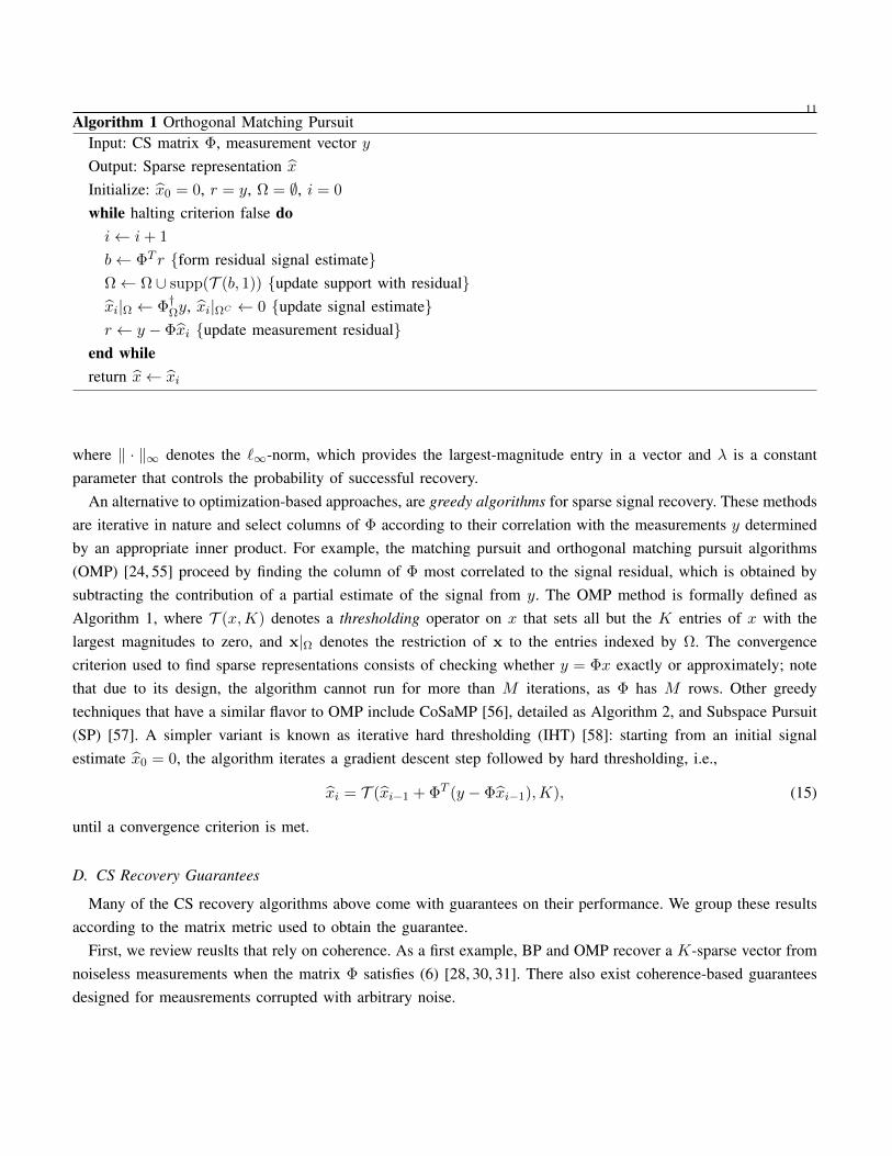
11Algorithm 1 Orthogonal Matching Pursuit

Input: CS matrix Φ, measurement vector yOutput: Sparse representation xInitialize: x0 = 0, r = y, Ω = ∅, i = 0

while halting criterion false doi← i+ 1

b← ΦT r form residual signal estimateΩ← Ω ∪ supp(T (b, 1)) update support with residualxi|Ω ← Φ†Ωy, xi|ΩC ← 0 update signal estimater ← y − Φxi update measurement residual

end whilereturn x← xi

where ‖ · ‖∞ denotes the `∞-norm, which provides the largest-magnitude entry in a vector and λ is a constantparameter that controls the probability of successful recovery.

An alternative to optimization-based approaches, are greedy algorithms for sparse signal recovery. These methodsare iterative in nature and select columns of Φ according to their correlation with the measurements y determinedby an appropriate inner product. For example, the matching pursuit and orthogonal matching pursuit algorithms(OMP) [24, 55] proceed by finding the column of Φ most correlated to the signal residual, which is obtained bysubtracting the contribution of a partial estimate of the signal from y. The OMP method is formally defined asAlgorithm 1, where T (x,K) denotes a thresholding operator on x that sets all but the K entries of x with thelargest magnitudes to zero, and x|Ω denotes the restriction of x to the entries indexed by Ω. The convergencecriterion used to find sparse representations consists of checking whether y = Φx exactly or approximately; notethat due to its design, the algorithm cannot run for more than M iterations, as Φ has M rows. Other greedytechniques that have a similar flavor to OMP include CoSaMP [56], detailed as Algorithm 2, and Subspace Pursuit(SP) [57]. A simpler variant is known as iterative hard thresholding (IHT) [58]: starting from an initial signalestimate x0 = 0, the algorithm iterates a gradient descent step followed by hard thresholding, i.e.,

xi = T (xi−1 + ΦT (y − Φxi−1),K), (15)

until a convergence criterion is met.

D. CS Recovery Guarantees

Many of the CS recovery algorithms above come with guarantees on their performance. We group these resultsaccording to the matrix metric used to obtain the guarantee.

First, we review reuslts that rely on coherence. As a first example, BP and OMP recover a K-sparse vector fromnoiseless measurements when the matrix Φ satisfies (6) [28, 30, 31]. There also exist coherence-based guaranteesdesigned for meausrements corrupted with arbitrary noise.

12Algorithm 2 CoSaMP

Input: CS matrix Φ, measurement vector y, sparsity KOutput: K-sparse approximation x to true signal xInitialize: x0 = 0, r = y, i = 0

while halting criterion false doi← i+ 1

e← ΦT r form residual signal estimateΩ← supp(T (e, 2K)) prune residualT ← Ω ∪ supp(xi−1) merge supportsb|T ← Φ†T y, b|TC ← 0 form signal estimatexi ← T (b,K) prune signal using modelr ← y − Φxi update measurement residual

end whilereturn x← xi

Theorem 5. [59] Let the signal x ∈ ΣK and write y = Φx + n. Denote γ = ‖n‖2. Suppose that K ≤(1/µ(Φ) + 1)/4 and ε ≥ γ in (12). Then the output x of (12) has error bounded by

‖x− x‖2 ≤γ + ε√

1− µ(Φ)(4K − 1), (16)

while the output x of the OMP algorithm with halting criterion ‖r‖2 ≤ γ has error bounded by

‖x− x‖2 ≤γ√

1− µ(Φ)(K − 1), (17)

provided that γ ≤ A(1 − µ(Φ)(2K − 1))/2 for OMP, with A being a positive lower bound on the magnitude ofthe nonzero entries of x.

Note here that BPIC must be aware of the noise magnitude γ to make ε ≥ γ, while OMP must be aware of thenoise magnitude γ to set an appropriate convergence criterion. Additionally, the error in Theorem 5 is proportionalto the noise magnitude γ. This is because the only assumption on the noise is its magnitude, so that n might bealigned to maximally harm the estimation process.

In the random noise case, bounds on ‖x − x‖2 can only be stated in high probability, since there is alwaysa small probability that the noise will be very large and completely overpower the signal. For example, underadditive white Gaussian noise (AWGN), the guarantees for BPIC in Theorems 5 hold with high probability when

the parameter ε = σ

√M + η

√2M , with η denoting an adjustable parameter to control the probability of ‖n‖2

being too large [60]. A second example gives a related result for the BPDN algorithm.

Theorem 6. [61] Let the signal x ∈ ΣK and write y = Φx+n, where n ∼ N (0, σ2I). Suppose that K < 1/3µ(Φ)

and consider the BPDN optimization problem (13) with λ =√

16σ2 logM . Then, with probability on the order

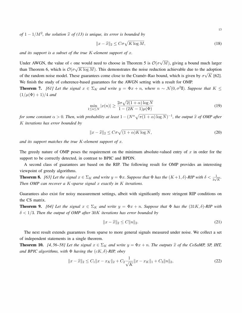
13

of 1− 1/M2, the solution x of (13) is unique, its error is bounded by

‖x− x‖2 ≤ Cσ√K logM, (18)

and its support is a subset of the true K-element support of x.

Under AWGN, the value of ε one would need to choose in Theorem 5 is O(σ√M), giving a bound much larger

than Theorem 6, which is O(σ√K logM). This demonstrates the noise reduction achievable due to the adoption

of the random noise model. These guarantees come close to the Cramer–Rao bound, which is given by σ√K [62].

We finish the study of coherence-based guarantees for the AWGN setting with a result for OMP.Theorem 7. [61] Let the signal x ∈ ΣK and write y = Φx + n, where n ∼ N (0, σ2I). Suppose that K ≤(1/µ(Φ) + 1)/4 and

min1≤n≤N

|x(n)| ≥ 2σ√

2(1 + α) logN

1− (2K − 1)µ(Φ)(19)

for some constant α > 0. Then, with probability at least 1− (Nα√π(1 + α) logN)−1, the output x of OMP after

K iterations has error bounded by

‖x− x‖2 ≤ Cσ√

(1 + α)K logN, (20)

and its support matches the true K-element support of x.

The greedy nature of OMP poses the requirement on the minimum absolute-valued entry of x in order for thesupport to be correctly detected, in contrast to BPIC and BPDN.

A second class of guarantees are based on the RIP. The following result for OMP provides an interestingviewpoint of greedy algorithms.Theorem 8. [63] Let the signal x ∈ ΣK and write y = Φx. Suppose that Φ has the (K+1, δ)-RIP with δ < 1

3√K

.Then OMP can recover a K-sparse signal x exactly in K iterations.

Guarantees also exist for noisy measurement settings, albeit with significantly more stringent RIP conditions onthe CS matrix.Theorem 9. [64] Let the signal x ∈ ΣK and write y = Φx + n. Suppose that Φ has the (31K, δ)-RIP withδ < 1/3. Then the output of OMP after 30K iterations has error bounded by

‖x− x‖2 ≤ C‖n‖2. (21)

The next result extends guarantees from sparse to more general signals measured under noise. We collect a setof independent statements in a single theorem.Theorem 10. [4, 56–58] Let the signal x ∈ ΣK and write y = Φx+ n. The outputs x of the CoSaMP, SP, IHT,and BPIC algorithms, with Φ having the (cK, δ)-RIP, obey

‖x− x‖2 ≤ C1‖x− xK‖2 + C21√K‖x− xK‖1 + C3‖n‖2, (22)

14

where xK = arg minx′∈ΣK‖x−x′‖2 is the best K-sparse approximation of the vector x when measured in the `2

norm. The requirements on the parameters c, δ of the RIP and the values of C1, C2, and C3 are specific to eachalgorithm. For example, for the BPIC algorithm, c = 2 and δ =

√2− 1 suffice to obtain the guarantee (22).

The type of guarantee given in Theorem 10 is known as uniform instance optimality, in the sense that the CSrecovery error is proportional to that of the best K-sparse approximation to the signal x for any signal x ∈ RN . Infact, the formulation of the CoSaMP, SP and IHT algorithms was driven by the goal of instance optimality, whichhas not been shown for older greedy algorithms like MP and OMP. Theorem 10 can also be adapted to recoveryof exactly sparse signals from noiseless measurements.

Corollary 11. Let the signal x ∈ ΣK and write y = Φx. The CoSaMP, SP, IHT, and BP algorithms can exactlyrecover x from y if Φ has the (cK, δ)-RIP, where the parameters c, δ of the RIP are specific to each algorithm.

Similarly to Theorem 5, the error in Theorem 10 is proportional to the noise magnitude ‖n‖2, and the boundscan be tailored to random noise with high probability. The Dantzig selector improves the scaling of the error inthe AWGN setting.

Theorem 12. [54] Let the signal x ∈ ΣK and write y = Φx + n, where n ∼ N (0, σ2I). Suppose that λ =√2(1+1/t) in (14) and that Φ has the (2K, δ2K) and (3K, δ3K)-RIPs with δ2K +δ3K < 1. Then, with probability

at least 1−N t/√π logN , we have

‖x− x‖2 ≤ C(1 + 1/t)2Kσ2 logN. (23)

Similar results under AWGN have been shown for the OMP and thresholding algorithms [61].A third class of guarantees relies on metrics additional to coherence and RIP. This class has a non-uniform flavor

in the sense that the results apply only for a certain subset of sufficiently sparse signals. Such flexibility allows forsignificant relaxations on the properties required from the matrix Φ. The next example has a probabilistic flavorand relies on the coherence property.Theorem 13. [65] Let the signal x ∈ ΣK with support drawn uniformly at random from the available

(NK

)

possibilities and entries drawn independently from a distribution P (X) so that P (X > 0) = P (X < 0). Writey = Φx and fix s ≥ 1 and 0 < δ < 1/2. If K ≤ log(N/δ)

8µ2(Φ) and√

18 logN

δlog

(K

2+ 1

)s+

2K

N‖Φ‖22 ≤ e−1/4

(1− 2−1/2

),

then x is the unique solution to BP (11) with probability at least 1− 2δ − (K/2)−s.

In words, the theorem says that as long as the coherence µ(Φ) and the spectral norm ‖Φ‖2 of the CS matrixare small enough, we will be able to recover the majority of K-sparse signals x from their measurements y.Probabilistic results that rely on coherence can also be obtained for the BPDN algorithm (13) [45].

The main difference between the guarantees that rely solely on coherence and those that rely on the RIP andprobabilistic sparse signal models is the scaling of the number of measurements M needed for successful recovery

15

of K-sparse signals. According to the bounds (8) and (9), the sparsity level that allows for recovery with highprobability in Theorems 10, 12, and 13 is K = O(M), compared with K = O(

√M) for the deterministic

guarantees provided by Theorems 5, 6, and 7. This so-called square root bottleneck [65] gives an additional reasonfor the popularity of randomized CS matrices and sparse signal models.

IV. STRUCTURE IN CS MATRICES

While most initial work in CS has emphasized the use of randomized CS matrices whose entries are obtainedindependently from a standard probability distribution, such matrices are often not feasible for real-world applica-tions due to the cost of multiplying arbitrary matrices with signal vectors of high dimension. In fact, very often thephysics of the sensing modality and the capabilities of sensing devices limit the types of CS matrices that can beimplemented in a specific application. Furthermore, in the context of analog sampling, one of the prime motivationsfor CS is to build analog samplers that lead to sub-Nyquist sampling rates. These involve actual hardware andtherefore structured sensing devices. Hardware considerations require more elaborate signal models to reduce thenumber of measurements needed for recovery as much as possible. In this section, we review available alternativesfor structured CS matrices; in each case, we provide known performance guarantees, as well as application areaswhere the structure arises. In Section VI we extend the CS framework to allow for analog sampling, and introducefurther structure into the measurement process. This results in new hardware implementations for reduced ratesamplers based on extended CS principles. Note that the survey of CS devices given in this section is by nomeans exhaustive [66–68]; our focus is on CS matrices that have been investigated from both a theoretical and animplementational point of view.

A. Subsampled Incoherent Bases

The key concept of a frame’s coherence can be extended to pairs of orthonormal bases. This enables a newchoice for CS matrices: one simply selects an orthonormal basis that is incoherent with the sparsity basis, andobtains CS measurements by selecting a subset of the coefficients of the signal in the chosen basis [69]. We notethat some degree of randomness remains in this scheme, due to the choice of coefficients selected to represent thesignal as CS measurements.

1) Formulation: Formally, we assume that a basis Φ ∈ RN×N is provided for measurement purposes, whereeach column of Φ = [φ1 φ2 . . . φN ] corresponds to a different basis element. Let Φ be an N ×M columnsubmatrix of Φ that preserves the basis vectors with indices Γ and set y = Φ

Tx. Under this setup, a different

metric arises to evaluate the performance of CS.

Definition 4. [28, 69] The mutual coherence of the N -dimensional orthonormal bases Φ and Ψ is the maximumabsolute value of the inner product between elements of the two bases:

µ(Φ,Ψ) = max1≤i,j≤N

|〈φi, ψj〉| , (24)

where ψj denotes the jth column, or element, of the basis Ψ.

The mutual coherence µ(Φ,Ψ) has values in the range[N−1/2, 1

]. For example, µ(Φ,Ψ) = N−1/2 when Φ

is the discrete Fourier transform basis, or Fourier matrix, and Ψ is the canonical basis, or identity matrix, and

16

µ(Φ,Ψ) = 1 when both bases share at least one element or column. Note also that the concepts of coherence andmutual coherence are connected by the equality µ(Φ,Ψ) = µ([Φ Ψ]). The definition of mutual coherence can alsobe extended to infinite-dimensional representations of continuous-time (analog) signals [33, 70].

2) Theoretical guarantees: The following theorem provides a recovery guarantee based on mutual coherence.Theorem 14. [69] Let x = Ψθ be a K-sparse signal in Ψ with support Ω ⊂ 1, . . . , N, |Ω| = K, and withentries having signs chosen uniformly at random. Choose a subset Γ ⊆ 1, . . . , N uniformly at random for the setof observed measurements, with M = |Γ|. Suppose that M ≥ CKNµ2(Φ,Ψ) log(N/δ) and M ≥ C ′ log2(N/δ)

for fixed values of δ < 1, C, C ′. Then with probability at least 1− δ, θ is the solution to (11).

The number of measurements required by Theorem 14 ranges from O(K logN) to O(N). It is possible toexpand the guarantee of Theorem 14 to compressible signals by adapting an argument of Rudelson and Vershyninin [71] to link coherence and restricted isometry constants.Theorem 15. [71, Remark 3.5.3] Choose a subset Γ ⊆ 1, . . . , N for the set of observed measurements, withM = |Γ|. Suppose that

M ≥ CK√Ntµ(Φ,Ψ) log(tK logN) log2K (25)

for a fixed value of C. Then with probability at least 1−5e−t the matrix ΦTΨ has the RIP with constant δ2K ≤ 1/2.

Using this theorem, we obtain the guarantee of Theorem 10 for compressible signals with the number ofmeasurements M dictated by the coherence value µ(Φ,Ψ).

3) Applications: There are two main categories of applications where subsampled incoherent bases are used. Inthe first category, the acquisition hardware is limited by construction to measure directly in a transform domain.The most relevant examples are magnetic resonance imaging (MRI) [72] and tomographic imaging [73], as wellas optical microscopy [74, 75]; in all of these cases, the measurements obtained from the hardware correspondto coefficients of the image’s 2-D continuous Fourier transform, albeit not typically selected in a randomizedfashion. Since the Fourier functions, corresponding to sinusoids, will be incoherent with functions that havelocalized support, this imaging approach works well in practice for sparsity/compressibility transforms such aswavelets [69], total variation [73], and the standard canonical representation [74].

In the case of optical microscopy, the Fourier coefficients that are measured correspond to the lowpass regime.The highpass values are completely lost. When the underlying signal x can change sign, standard sparse recoveryalgorithms such as BP do not typically succeed in recovering the true underlying vector. To treat the case ofrecovery from lowpass coefficients, a special purpose sparse recovery method was developed under the name ofNonlocal Hard Thresholding (NLHT) [74]. This technique attempts to allocate the off-support of the sparse signalin an iterative fashion by performing a thresholding step that depends on the values of the neighboring locations.

The second category involves the design of new acquisition hardware that can obtain projections of the signalagainst a class of vectors. The goal of the matrix design step is to find a basis whose elements belong to theclass of vectors that can be implemented on the hardware. For example, a class of single pixel imagers basedon optical modulators [60, 76] (see an example in Fig. 1) can obtain projections of an image against vectors thathave binary entries. Example bases that meet this criterion include the Walsh-Hadamard and noiselet bases [77].The latter is particularly interesting for imaging applications, as it is known to be maximally incoherent with the

17

A/D

DMDArray

Photodiode

Reconstruction

Scene

Bitstream

Image

Fig. 1. Diagram of the single pixel camera. The incident lightfield (corresponding to the desired image x) is reflected off a digital micro-mirrordevice (DMD) array whose mirror orientations are modulated in the pseudorandom pattern supplied by the random number generator (RNG).Each different mirror pattern produces a voltage at the single photodiode that corresponds to one measurement y(m). The process is repeatedwith different patterns M times to obtain a full measurement vector y (taken from [76]).

Haar wavelet basis. In contrast, certain elements of the Walsh-Hadamard basis are highly coherent with waveletfunctions at coarse scales, due to their large supports. Permuting the entries of the basis vectors (in a random orpseudorandom fashion) helps reduce the coherence between the measurement basis and a wavelet basis. Becausethe single pixel camera modulates the light field through optical aggregation, it improves the signal-to-noise ratioof the measurements obtained when compared to standard multisensor schemes [78]. Similar imaging hardwarearchitectures have been developed in [79, 80].

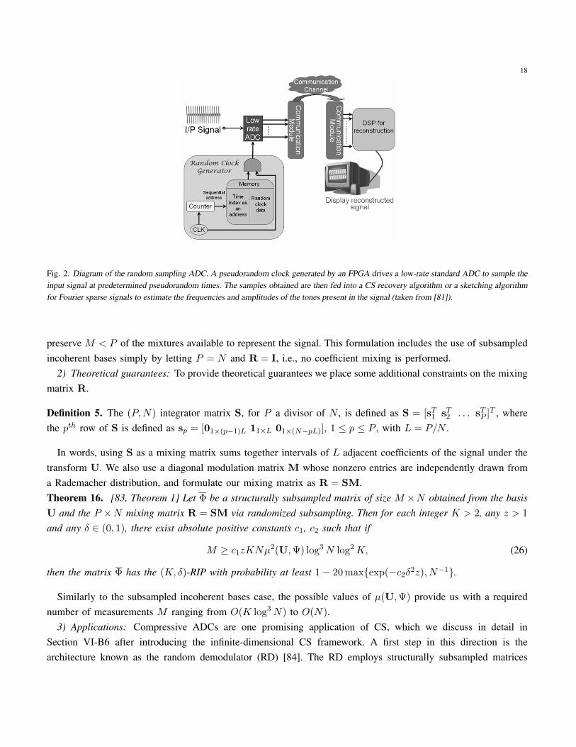
An additional example of a configurable acquisition device is the random sampling ADC [81], which is designedfor acquisition of periodic, multitone analog signals whose frequency components belong to a uniform grid(similarly to the random demodulator of Section IV-B3). The sparsity basis for the signal once again is chosento be the discrete Fourier transform basis. The measurement basis is chosen to be the identity basis, so that themeasurements correspond to standard signal samples taken at randomized times. The hardware implementationemploys a randomized clock that drives a traditional low-rate ADC to sample the input signal at specific times.As shown in Fig. 2, the random clock is implemented using an FPGA that outputs a predetermined pseudorandompulse sequence indicating the times at which the signal is sampled. The patterns are timed according to a set ofpseudorandom arithmetic progressions. This process is repeated cyclically, establishing a windowed acquisitionfor signals of arbitrary length. The measurement and sparsity framework used by this randomized ADC is alsocompatible with sketching algorithms designed for signals that are sparse in the frequency domain [81, 82].

B. Structurally Subsampled Matrices

In certain applications, the measurements obtained by the acquisition hardware do not directly correspond to thesensed signal’s coefficients in a particular transform. Rather, the observations are a linear combination of multiplecoefficients of the signal. The resulting CS matrix has been termed a structurally subsampled matrix [83].

1) Formulation: Consider a matrix of available measurement vectors that can be described as the productΦ = RU, where R is a P ×N mixing matrix and U is a basis. The CS matrix Φ is obtained by selecting M outof P rows at random, and normalizing the columns of the resulting subsampled matrix. There are two possibledownsampling stages: first, R might offer only P < N mixtures to be available as measurements; second, we only

18

Fig. 2. Diagram of the random sampling ADC. A pseudorandom clock generated by an FPGA drives a low-rate standard ADC to sample theinput signal at predetermined pseudorandom times. The samples obtained are then fed into a CS recovery algorithm or a sketching algorithmfor Fourier sparse signals to estimate the frequencies and amplitudes of the tones present in the signal (taken from [81]).

preserve M < P of the mixtures available to represent the signal. This formulation includes the use of subsampledincoherent bases simply by letting P = N and R = I, i.e., no coefficient mixing is performed.

2) Theoretical guarantees: To provide theoretical guarantees we place some additional constraints on the mixingmatrix R.

Definition 5. The (P,N) integrator matrix S, for P a divisor of N , is defined as S = [sT1 sT2 . . . sTP ]T , wherethe pth row of S is defined as sp = [01×(p−1)L 11×L 01×(N−pL)], 1 ≤ p ≤ P , with L = P/N .

In words, using S as a mixing matrix sums together intervals of L adjacent coefficients of the signal under thetransform U. We also use a diagonal modulation matrix M whose nonzero entries are independently drawn froma Rademacher distribution, and formulate our mixing matrix as R = SM.Theorem 16. [83, Theorem 1] Let Φ be a structurally subsampled matrix of size M ×N obtained from the basisU and the P ×N mixing matrix R = SM via randomized subsampling. Then for each integer K > 2, any z > 1

and any δ ∈ (0, 1), there exist absolute positive constants c1, c2 such that if

M ≥ c1zKNµ2(U,Ψ) log3N log2K, (26)

then the matrix Φ has the (K, δ)-RIP with probability at least 1− 20 maxexp(−c2δ2z), N−1.

Similarly to the subsampled incoherent bases case, the possible values of µ(U,Ψ) provide us with a requirednumber of measurements M ranging from O(K log3N) to O(N).

3) Applications: Compressive ADCs are one promising application of CS, which we discuss in detail inSection VI-B6 after introducing the infinite-dimensional CS framework. A first step in this direction is thearchitecture known as the random demodulator (RD) [84]. The RD employs structurally subsampled matrices

19

PseudorandomNumberGenerator

Seed

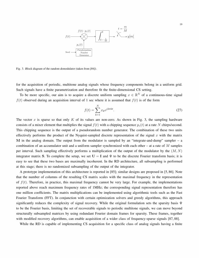
Fig. 3. Block diagram of the random demodulator (taken from [84]).

for the acquisition of periodic, multitone analog signals whose frequency components belong in a uniform grid.Such signals have a finite parametrization and therefore fit the finite-dimensional CS setting.

To be more specific, our aim is to acquire a discrete uniform sampling x ∈ RN of a continuous-time signalf(t) observed during an acquisition interval of 1 sec where it is assumed that f(t) is of the form

f(t) =

N∑

k=1

xkej2πkt. (27)

The vector x is sparse so that only K of its values are non-zero. As shown in Fig. 3, the sampling hardwareconsists of a mixer element that multiplies the signal f(t) with a chipping sequence pc(t) at a rate N chirps/second.This chipping sequence is the output of a pseudorandom number generator. The combination of these two unitseffectively performs the product of the Nyquist-sampled discrete representation of the signal x with the matrixM in the analog domain. The output from the modulator is sampled by an “integrate-and-dump” sampler – acombination of an accumulator unit and a uniform sampler synchronized with each other – at a rate of M samplesper interval. Such sampling effectively performs a multiplication of the output of the modulator by the (M,N)

integrator matrix S. To complete the setup, we set U = I and Ψ to be the discrete Fourier transform basis; it iseasy to see that these two bases are maximally incoherent. In the RD architecture, all subsampling is performedat this stage; there is no randomized subsampling of the output of the integrator.

A prototype implementation of this architecture is reported in [85]; similar designs are proposed in [5, 86]. Notethat the number of columns of the resulting CS matrix scales with the maximal frequency in the representationof f(t). Therefore, in practice, this maximal frequency cannot be very large. For example, the implementationsreported above reach maximum frequency rates of 1MHz; the corresponding signal representation therefore hasone million coefficients. The matrix multiplications can be implemented using algorithmic tools such as the FastFourier Transform (FFT). In conjunction with certain optimization solvers and greedy algorithms, this approachsignificantly reduces the complexity of signal recovery. While the original formulation sets the sparsity basis Ψ

to be the Fourier basis, limiting the set of recoverable signals to periodic multitone signals, we can move beyondstructurally subsampled matrices by using redundant Fourier domain frames for sparsity. These frames, togetherwith modified recovery algorithms, can enable acquisition of a wider class of frequency-sparse signals [87, 88].

While the RD is capable of implementing CS acquisition for a specific class of analog signals having a finite

20

parametrization, the CS framework can be adapted to infinite-dimensional signal models, enabling more efficientanalog acquisition and digital processing architectures. We defer the details to Section VI.

C. Subsampled Circulant Matrices

The use of Toeplitz and circulant structures [89–91] as CS matrices was first inspired by applications incommunications – including channel estimation and multi-user detection – where a sparse prior is placed onthe signal to be estimated, such as a channel response or a multiuser activity pattern. When compared with genericCS matrices, subsampled circulant matrices have a significantly smaller number of degrees of freedom due to therepetition of the matrix entries along the rows and columns.

1) Formulation: A circulant matrix U is a square matrix where the entries in each diagonal are all equal, andwhere the first entry of the second and subsequent rows is equal to the last entry of the previous row. Sincethis matrix is square, we perform random subsampling of the rows (in a fashion similar to that described inSection IV-B) to obtain a CS matrix Φ = RU, where R is an M × N subsampling matrix, i.e., a submatrix ofthe identity matrix. We dub Φ a subsampled circulant matrix.

2) Theoretical guarantees: Even when the sequence defining U is drawn at random from the distributionsdescribed in Section III, the particular structure of the subsampled circulant matrix Φ = RU prevents the use ofthe proof techniques used in standard CS, which require all entries of the matrix to be independent. However, itis possible to employ different probabilistic tools to provide guarantees for subsampled circulant matrices. Theresults still require randomness in the selection of the entries of the circulant matrix.Theorem 17. [91] Let Φ be a subsampled circulant matrix whose distinct entries are independent randomvariables following a Rademacher distribution, and R is an arbitrary M ×N identity submatrix. Furthermore, letδ be the smallest value for which (7) holds for all x ∈ ΣK . Then for δ0 ∈ (0, 1) we have E[δ] ≤ δ0 provided that

M ≥ Cmaxδ−10 K3/2 log3/2N, δ−2

0 K log2N log2K,

where C > 0 is a universal constant. Furthermore, for 0 ≤ λ ≤ 1,

P(δK ≥ E[δ] + λ) ≤ eλ2/σ2

, where σ2 = C ′K

Mlog2K logN,

for a universal constant C ′ > 0.

In words, if we have M = O(K1.5 log1.5N

), then the RIP required for Φ by many algorithms for successful

recovery is achieved with high probability.3) Applications: There are several sensing applications where the signal to be acquired is convolved with

the sampling hardware’s impulse response before it is measured. Additionally, because convolution is equivalentto a product operator in the Fourier domain, it is possible to speed up the CS recovery process by performingmultiplications by the matrices Φ and ΦT via the FFT. In fact, such an FFT-based procedure can also be exploited togenerate good CS matrices [92]. First, we design a matrix Φ in the Fourier domain to be diagonal and have entriesdrawn from a suitable probability distribution. Then, we obtain the measurement matrix Φ by subsampling thematrix Φ, similarly to the incoherent basis case. While this formulation assumes that the convolution during signalacquisition is circulant, this gap between theory and practice has been studied and shown to be controllable [93].

21

20

40

60

80

100

20

40

60

80

100

0

1000

2000

3000

4000

5000

(a) Coding pattern h(MURA) (b) Decoding pattern h(MURA) (c) Convolution h(MURA) ∗ h(MURA)

Figure 1. The MURA pattern for a 101×101 grid. (a) The white blocks are openings (b) The decoding pattern for (a) is nearly identical.(c) If the white blocks have value 1 and the black blocks have value 0, and the blue blocks in (b) have value −1, then the convolution ofthe matrices corresponding to this two patterns appear like a Kronecker-δ function.

holds for all subsets T with |T | ≤ 3m.8 An observation matrix R satisfying RIP with high probability is often referredto as a compressed sensing (CS) matrix. While the RIP cannot be verified for a given R, it has been shown that matriceswith entries drawn independently from some probability distributions satisfy the condition with high probability whenk ≥ Cm log(N/m) for some constant C, where m ≡ θt 0 is the number of non-zero elements in the vector θt .8

We observe yt = Rtθt + nt, where nt is white Gaussian noise. The 2 − 1 minimization

θt = arg minθt

1

2yt −Rtθt22 + τθt1 (3)

ft = W θt

will yield a highly accurate estimate of ft with very high probability.4, 11 The regularization parameter τ > 0 helps to

overcome the ill-posedness of the problem, and the 1 penalty term drives small components of θ to zero and helps createsparse solutions.

2.3.2 Coded apertures for compressed sensing

We have previously designed a coded aperture imaging mask, denoted h(CCA), such that the corresponding observationmatrix Rt satisfies the RIP.6 The measurement matrix At (recall Rt = AtW ) associated with compressive coded apertures(CCA) can be modeled as

A(CCA)t f

t = D(ft ∗ h(CCA)) (4)

where D is a downsampling operator induced by the FPA which consists of partitioning ft ∗h(CCA) into k uniformly sized

blocks and measuring the total intensity in each block. (This is sometimes referred to as integration downsampling.) Inthis case the operator At is independent of t, but we do not reflect this in the notation to be consistent throughout the paper.

The convolution of h(CCA) with a signal ft as in (4) can be computed by applying the Fourier transform F to f

t

and h(CCA), then performing element-wise matrix multiplication, and then mapping the product using the Fourier inversetransform. In linear algebra notation, this series of operation can be expressed as

h(CCA) ∗ ft = F−1CHF f

t ,

where F is the two-dimensional Fourier transform matrix, and CH is the diagonal matrix whose diagonal elements cor-respond to the transfer function H = F (h(CCA)). (This is a slight abuse of notation, since on the left hand side f

t is animage, and on the right hand side f

t is a vectorized representation of an image.) The coded aperture masks are designedso that A

(CCA)t satisfies RIP as described in (2). Specifically, the authors developed a method for randomly generating a

mask h(CCA) so that the corresponding matrix product F−1CHF is block-circulant and each block was in turn circulant,

(a) (b)

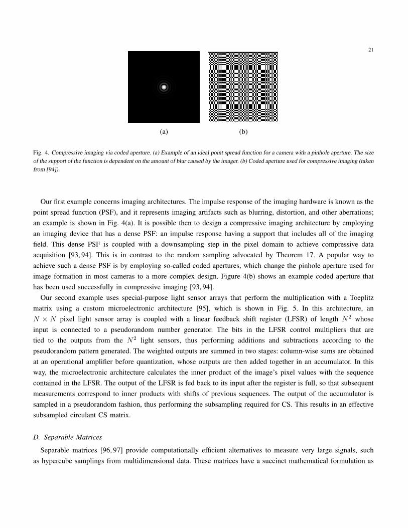
Fig. 4. Compressive imaging via coded aperture. (a) Example of an ideal point spread function for a camera with a pinhole aperture. The sizeof the support of the function is dependent on the amount of blur caused by the imager. (b) Coded aperture used for compressive imaging (takenfrom [94]).

Our first example concerns imaging architectures. The impulse response of the imaging hardware is known as thepoint spread function (PSF), and it represents imaging artifacts such as blurring, distortion, and other aberrations;an example is shown in Fig. 4(a). It is possible then to design a compressive imaging architecture by employingan imaging device that has a dense PSF: an impulse response having a support that includes all of the imagingfield. This dense PSF is coupled with a downsampling step in the pixel domain to achieve compressive dataacquisition [93, 94]. This is in contrast to the random sampling advocated by Theorem 17. A popular way toachieve such a dense PSF is by employing so-called coded apertures, which change the pinhole aperture used forimage formation in most cameras to a more complex design. Figure 4(b) shows an example coded aperture thathas been used successfully in compressive imaging [93, 94].

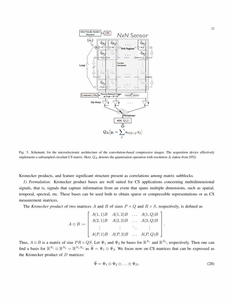
Our second example uses special-purpose light sensor arrays that perform the multiplication with a Toeplitzmatrix using a custom microelectronic architecture [95], which is shown in Fig. 5. In this architecture, anN × N pixel light sensor array is coupled with a linear feedback shift register (LFSR) of length N2 whoseinput is connected to a pseudorandom number generator. The bits in the LFSR control multipliers that aretied to the outputs from the N2 light sensors, thus performing additions and subtractions according to thepseudorandom pattern generated. The weighted outputs are summed in two stages: column-wise sums are obtainedat an operational amplifier before quantization, whose outputs are then added together in an accumulator. In thisway, the microelectronic architecture calculates the inner product of the image’s pixel values with the sequencecontained in the LFSR. The output of the LFSR is fed back to its input after the register is full, so that subsequentmeasurements correspond to inner products with shifts of previous sequences. The output of the accumulator issampled in a pseudorandom fashion, thus performing the subsampling required for CS. This results in an effectivesubsampled circulant CS matrix.

D. Separable Matrices

Separable matrices [96, 97] provide computationally efficient alternatives to measure very large signals, suchas hypercube samplings from multidimensional data. These matrices have a succinct mathematical formulation as

22

Fig. 5. Schematic for the microelectronic architecture of the convolution-based compressive imager. The acquisition device effectivelyimplements a subsampled circulant CS matrix. Here, Q∆ denotes the quantization operation with resolution ∆ (taken from [95]).

Kronecker products, and feature significant structure present as correlations among matrix subblocks.1) Formulation: Kronecker product bases are well suited for CS applications concerning multidimensional

signals, that is, signals that capture information from an event that spans multiple dimensions, such as spatial,temporal, spectral, etc. These bases can be used both to obtain sparse or compressible representations or as CSmeasurement matrices.

The Kronecker product of two matrices A and B of sizes P ×Q and R× S, respectively, is defined as

A⊗B :=

A(1, 1)B A(1, 2)B . . . A(1, Q)B

A(2, 1)B A(2, 2)B . . . A(2, Q)B...

.... . .

...A(P, 1)B A(P, 2)B . . . A(P,Q)B

.

Thus, A⊗B is a matrix of size PR×QS. Let Ψ1 and Ψ2 be bases for RN1 and RN2 , respectively. Then one canfind a basis for RN1 ⊗ RN2 = RN1N2 as Ψ = Ψ1 ⊗ Ψ2. We focus now on CS matrices that can be expressed asthe Kronecker product of D matrices:

Φ = Φ1 ⊗ Φ2 ⊗ . . .⊗ ΦD. (28)

23

If we denote the size of Φd as Md×Nd, then the matrix Φ has size M×N , with M =∏Dd=1Md and N =

∏Dd=1Nd.

Next, we describe the use of Kronecker product matrices in CS of multidimensional signals. We denote theentries of a D-dimensional signal x by x(n1, . . . , nd). We call the restriction of a multidimensional signal to fixedindices for all but its dth dimension a d-section of the signal. For example, for a 3-D signal x ∈ RN1×N2×N3 , thevector xi,j,· := [x(i, j, 1) x(i, j, 2) . . . x(i, j,N3)] is a 3-section of x.

Kronecker product sparsity bases make it possible to simultaneously exploit the sparsity properties of a multidi-mensional signal along each of its dimensions. The new basis is simply the Kronecker product of the bases usedfor each of its d-sections. More formally, we let x ∈ RN1 ⊗ . . . ⊗ RND = RN1×...×ND = R

∏Dd=1Nd and assume

that each d-section is sparse or compressible in a basis Ψd. We then define a sparsity/compressibility basis for xas Ψ = Ψ1 ⊗ . . .⊗ΨD, and obtain a coefficient vector θ for the signal ensemble so that x = Ψ θ, where x is acolumn vector-reshaped representation of x. We then have y = Φx = Φ Ψ θ.

2) Theoretical guarantees: Due to the similarity between blocks of Kronecker product CS matrices, it is easyto obtain bounds for their performance metrics. Our first result concerns the RIP.Lemma 3. [96, 97] Let Φd, 1 ≤ d ≤ D, be matrices that have the (K, δd)-RIP, 1 ≤ d ≤ D, respectively. ThenΦ, defined in (28), has the (K, δ)-RIP, with

δ ≤D∏

d=1

(1 + δd)− 1. (29)

When Φd is an orthonormal basis, it has the (K, δd)-RIP with δd = 0 for all K ≤ N . Therefore the RIP constantof the Kronecker product of an orthonormal basis and a CS matrix is equal to the RIP constant of the CS matrix.

It is also possible to obtain results on mutual coherence (described in Section III) for cases in which the basisused for sparsity or compressibility can also be expressed as a Kronecker product.Lemma 4. [96, 97] Let Φd, Ψd be bases for RNd for d = 1, . . . , D. Then

µ(Φ,Ψ) =

D∏

d=1

µ(Φd,Ψd). (30)

Lemma 4 provides a conservation of mutual coherence across Kronecker products. Since the mutual coherenceof each d-section’s sparsity and measurement bases is upper bounded by one, the number of Kronecker product-based measurements necessary for successful recovery of the multidimensional signal (following Theorems 14and 15) is always lower than or equal to the corresponding number of necessary partitioned measurements thatprocess only a portion of the multidimensional signal along its dth dimension at a time, for some d ∈ 1, . . . , D.This reduction is maximized when the d-section measurement basis Φ is maximally incoherent with the d-sectionsparsity basis Ψ.

3) Applications: Most applications of separable CS matrices involve multidimensional signals such as videosequences and hyperspectral datacubes. Our first example is an extension of the single pixel camera (see Fig. 1)to hyperspectral imaging [98]. The aim here is to record the reflectivity of a scene at different wavelengths; eachwavelength has a corresponding spectral frame, so that the hyperspectral datacube can be essentially interpreted asthe stacking of a sequence of images corresponding to the different spectra. The single pixel hyperspectral camera

24

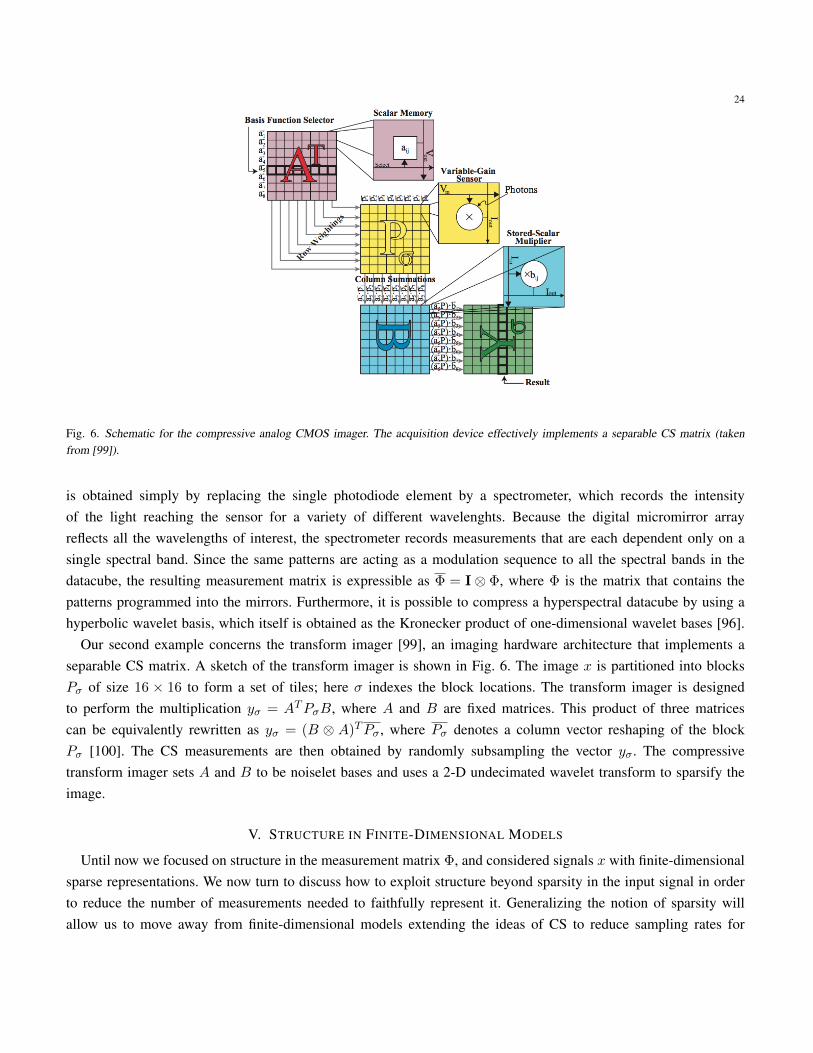
Fig. 6. Schematic for the compressive analog CMOS imager. The acquisition device effectively implements a separable CS matrix (takenfrom [99]).

is obtained simply by replacing the single photodiode element by a spectrometer, which records the intensityof the light reaching the sensor for a variety of different wavelenghts. Because the digital micromirror arrayreflects all the wavelengths of interest, the spectrometer records measurements that are each dependent only on asingle spectral band. Since the same patterns are acting as a modulation sequence to all the spectral bands in thedatacube, the resulting measurement matrix is expressible as Φ = I⊗ Φ, where Φ is the matrix that contains thepatterns programmed into the mirrors. Furthermore, it is possible to compress a hyperspectral datacube by using ahyperbolic wavelet basis, which itself is obtained as the Kronecker product of one-dimensional wavelet bases [96].

Our second example concerns the transform imager [99], an imaging hardware architecture that implements aseparable CS matrix. A sketch of the transform imager is shown in Fig. 6. The image x is partitioned into blocksPσ of size 16 × 16 to form a set of tiles; here σ indexes the block locations. The transform imager is designedto perform the multiplication yσ = ATPσB, where A and B are fixed matrices. This product of three matricescan be equivalently rewritten as yσ = (B ⊗ A)TPσ, where Pσ denotes a column vector reshaping of the blockPσ [100]. The CS measurements are then obtained by randomly subsampling the vector yσ. The compressivetransform imager sets A and B to be noiselet bases and uses a 2-D undecimated wavelet transform to sparsify theimage.

V. STRUCTURE IN FINITE-DIMENSIONAL MODELS

Until now we focused on structure in the measurement matrix Φ, and considered signals x with finite-dimensionalsparse representations. We now turn to discuss how to exploit structure beyond sparsity in the input signal in orderto reduce the number of measurements needed to faithfully represent it. Generalizing the notion of sparsity willallow us to move away from finite-dimensional models extending the ideas of CS to reduce sampling rates for

25

infinite-dimensional continuous-time signals, which is the main goal of sampling theory.We begin our discussion in this section within the finite-dimensional context by adding structure to the non-zero

values of x. We will then turn, in Section VI, to more general, infinite-dimensional notions of structure, that canbe applied to a broader class of analog signals.

A. Multiple Measurement Vectors

Historically, the first class of structure that has been considered within the CS framework has been that of multiplemeasurement vectors (MMVs) [101] which, similarly to sparse approximation, has been an area of interest in signalprocessing for more than a decade [21]. In this setting, rather than trying to recover a single sparse vector x, thegoal is to jointly recover a set of vectors xiLi=1 that share a common support. Stacking these vectors into thecolumns of a matrix X, there will be at most K non-zero rows in X. That is, not only is each vector K-sparse,but the non-zero values occur on a common location set. We use the notation Ω = supp(X) to denote the set ofindices of the non-zero rows.

MMV problems appear quite naturally in many different applications areas. Early work on MMV algorithmsfocused on magnetoencephalography, which is a modality for imaging the brain [21, 102]. Similar ideas were alsodeveloped in the context of array processing [21, 103, 104], equalization of sparse communication channels [105,106], and more recently cognitive radio and multiband communications [9, 86, 107–109].

1) Conditions on measurement matrices: As in standard CS, we assume that we are given measurements yiLi=1

where each vector is of length M < N . Letting Y be the M×L matrix with columns yi, our problem is to recoverX assuming a known measurement matrix Φ so that Y = ΦX. Clearly, we can apply any CS method to recoverxi from yi as before. However, since the vectors xi all have a common support, we expect intuitively to improvethe recovery ability by exploiting this joint information. In other words, we should in general be able to reducethe number of measurements ML needed to represent X below SL, where S is the number of measurementsrequired to recover one vector xi for a given matrix Φ.

Since |Ω| = K, the rank of X satisfies rank(X) ≤ K. When rank(X) = 1, all the sparse vectors xi aremultiples of each other, so that there is no advantage to their joint processing. However, when rank(X) is large,we expect to be able to exploit the diversity in its columns in order to benefit from joint recovery. This essentialresult is captured by the following necessary and sufficient uniqueness condition:Theorem 18. [110] A necessary and sufficient condition for the measurements Y = ΦX to uniquely determinethe jointly sparse matrix X is that

| supp(X)| < spark(Φ)− 1 + rank(X)

2. (31)

The sufficiency result was initially shown for the case rank(X) = | supp(X)| [111]. As shown in [110, 112],we can replace rank(X) by rank(Y) in (31). The sufficient direction of this condition was shown in [113] tohold even in the case where there are infinitely many vectors xi. A direct consequence of Theorem 18 is thatmatrices X with larger rank can be recovered from fewer measurements. Alternatively, matrices X with largersupport can be recovered from the same number of measurements. When rank(X) = K and spark(Φ) takes on itslargest possible value equal to M + 1, condition (31) becomes M ≥ K + 1. Therefore, in this best-case scenario,only K + 1 measurements per signal are needed to ensure uniqueness. This is much lower than the value of 2K

26

obtained in standard CS via the spark (cf. Theorem 4), which we refer to here as the single measurement vector(SMV) setting. Furthermore, as we now show, in the noiseless setting X can be recovered by a simple algorithm,in contrast to the combinatorial complexity needed to solve the SMV problem from 2K measurements for generalmatrices Φ.

2) Recovery Algorithms: A variety of algorithms have been proposed that exploit the joint sparsity in differentways. As in the SMV setting, two main approaches to solving MMV problems are based on convex optimizationand greedy methods. The analogue of (10) in the MMV case is

X = arg minX∈RN×L

‖X‖0,q subject to Y = ΦX, (32)

where we define the `p,q norms for matrices as

‖X‖p,q =

(∑

i

‖xi‖qp

)1/q

(33)

with xi denoting the ith row of X. With a slight abuse of notation, we also consider the quasi-norms with p = 0

such that ‖X‖0,q = | supp(X)| for any q. Optimization based algorithms relax the `0 norm in (32) and attempt torecover X by mixed norm minimization [17, 112, 114–117]:

X = arg minX∈RN×L

‖X‖p,q subject to Y = ΦX (34)

for some p, q ≥ 1; values of p, q = 1, 2 and ∞ have been advocated.The standard greedy approaches in the SMV setting have also been extended to the MMV case [101, 110, 114,

118–120]. The basic idea is to replace the residual vector r by a residual matrix R, which contains the residualswith respect to each of the measurements, and to replace the surrogate vector ΦT r by the q-norms of the rowsof ΦTR. For example, making these changes to OMP (Algorithm 1) yields a variant known as simultaneousorthogonal matching pursuit, shown as Algorithm 3, where X|Ω denotes the restriction of X to the rows indexedby Ω.

An alternative MMV strategy is the ReMBo (reduce MMV and boost) algorithm [113]. ReMBo first reduces theproblem to an SMV that preserves the sparsity pattern, and then recovers the signal support set; given the support,the measurements can be inverted to recover the input. The reduction is performed by merging the measurementcolumns with random coefficients. The details of the approach together with a recovery guarantee are given in thefollowing theorem.

Theorem 19. Let X be the unique K-sparse solution matrix of Y = ΦX and let Φ have spark greater than 2K.Let a be a random vector with an absolutely continuous distribution and define the random vectors y = Ya andx = Xa. Consider the random SMV system y = Φx. Then:

1) for every realization of a, the vector x is the unique K-sparse solution of the SMV;2) Ω(x) = Ω(X) with probability one.

According to Theorem 19, the MMV problem is first reduced to an SMV counterpart, for which the optimalsolution x is found. We then choose the support of X to be equal to that of x, and invert the measurement vectorsY over this support. In practice, computationally efficient methods are used to solve the SMV counterpart, which

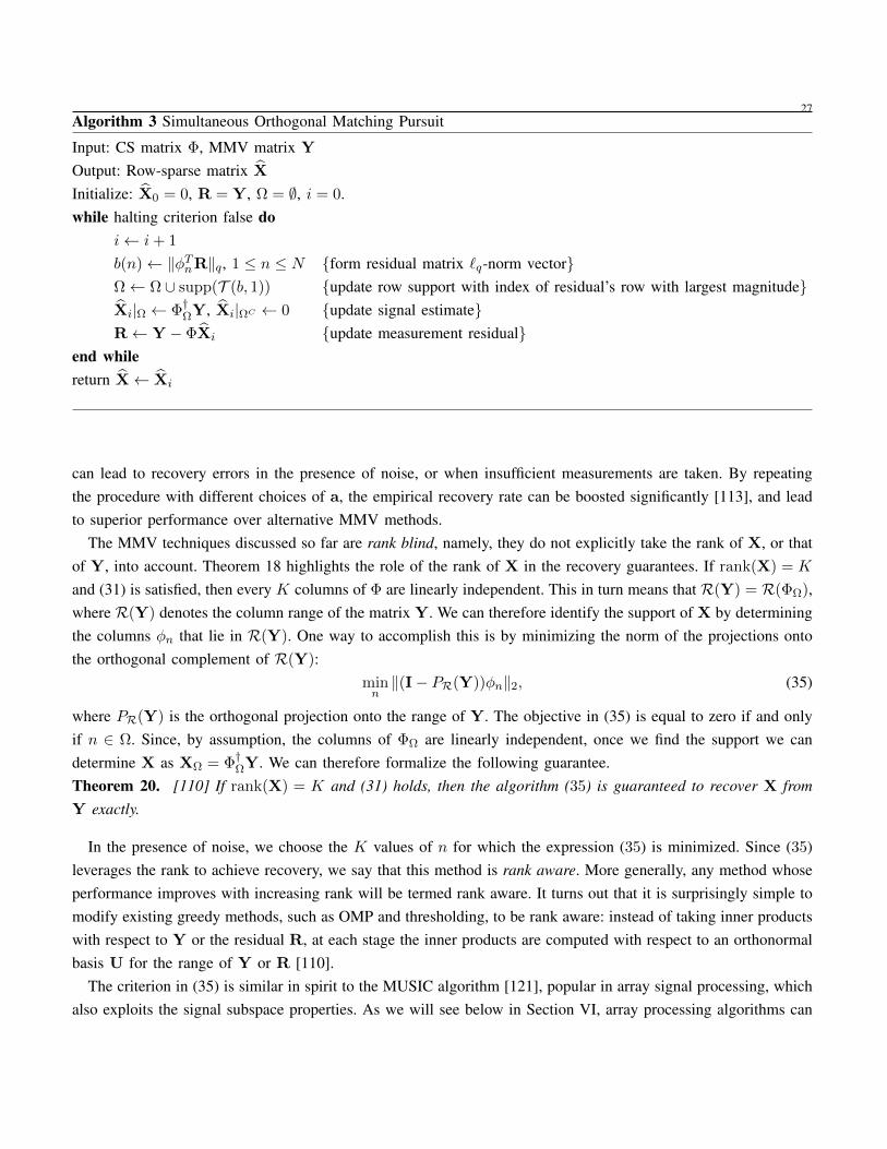
27Algorithm 3 Simultaneous Orthogonal Matching Pursuit

Input: CS matrix Φ, MMV matrix Y

Output: Row-sparse matrix X

Initialize: X0 = 0, R = Y, Ω = ∅, i = 0.while halting criterion false do

i← i+ 1

b(n)← ‖φTnR‖q, 1 ≤ n ≤ N form residual matrix `q-norm vectorΩ← Ω ∪ supp(T (b, 1)) update row support with index of residual’s row with largest magnitudeXi|Ω ← Φ†ΩY, Xi|ΩC ← 0 update signal estimateR← Y − ΦXi update measurement residual

end whilereturn X← Xi

can lead to recovery errors in the presence of noise, or when insufficient measurements are taken. By repeatingthe procedure with different choices of a, the empirical recovery rate can be boosted significantly [113], and leadto superior performance over alternative MMV methods.

The MMV techniques discussed so far are rank blind, namely, they do not explicitly take the rank of X, or thatof Y, into account. Theorem 18 highlights the role of the rank of X in the recovery guarantees. If rank(X) = K

and (31) is satisfied, then every K columns of Φ are linearly independent. This in turn means that R(Y) = R(ΦΩ),where R(Y) denotes the column range of the matrix Y. We can therefore identify the support of X by determiningthe columns φn that lie in R(Y). One way to accomplish this is by minimizing the norm of the projections ontothe orthogonal complement of R(Y):

minn‖(I− PR(Y))φn‖2, (35)

where PR(Y) is the orthogonal projection onto the range of Y. The objective in (35) is equal to zero if and onlyif n ∈ Ω. Since, by assumption, the columns of ΦΩ are linearly independent, once we find the support we candetermine X as XΩ = Φ†ΩY. We can therefore formalize the following guarantee.Theorem 20. [110] If rank(X) = K and (31) holds, then the algorithm (35) is guaranteed to recover X fromY exactly.

In the presence of noise, we choose the K values of n for which the expression (35) is minimized. Since (35)leverages the rank to achieve recovery, we say that this method is rank aware. More generally, any method whoseperformance improves with increasing rank will be termed rank aware. It turns out that it is surprisingly simple tomodify existing greedy methods, such as OMP and thresholding, to be rank aware: instead of taking inner productswith respect to Y or the residual R, at each stage the inner products are computed with respect to an orthonormalbasis U for the range of Y or R [110].

The criterion in (35) is similar in spirit to the MUSIC algorithm [121], popular in array signal processing, whichalso exploits the signal subspace properties. As we will see below in Section VI, array processing algorithms can

28

be used to treat a variety of other structured analog sampling problems.The MMV model can be further extended to include the case in which there are possibly infinitely many

measurement vectorsy(λ) = Φx(λ), λ ∈ Λ, (36)

where Λ indicates an appropriate index set (which can be countable or uncountable). Here again the assumptionis that the set of vectors x(λ), λ ∈ Λ all have common support Ω of size K. Such an infinite-set of equationsis referred to as an infinite measurement vector (IMV) system. The common, finite, support set can be exploitedin order to recover x(λ) efficiently by solving an MMV problem [113] Reduction to a finite MMV counterpart isperformed via the continuous to finite (CTF) block, which aims at robust detection of Ω. The CTF builds a frame(or a basis) from the measurements using

y(λ)Frame construct−−−−−−−−−−→ Q =

∑

λ∈Λ

y(λ)yH(λ)

Decompose−−−−−−−→ Q = VVH . (37)

Typically, Q is constructed from roughly 2K snapshots y(λ), and the (optional) decomposition allows removalof the noise space [109]. Once the basis V is determined, the CTF solves an MMV system V = ΦU withsupp(U) ≤ K. An alternative approach based on the MUSIC algorithm was suggested in [111, 122].

The crux of the CTF is that the indices of the nonidentically-zero rows of the matrix U that solves the finiteunderdetermined system V = ΦU coincide with the index set Ω that is associated with the infinite signal-setx(λ) [113], as incoporated in the follwoing theorem.

Theorem 21. [109] Suppose that the system of equations (36) has a unique K-sparse solution set with support Ω,and that the matrix Φ satisfies (31). Let V be a matrix whose column span is equal to the span of y(λ), λ ∈ Λ.Then, the linear system V = ΦU has a unique K-sparse solution with row support equal Ω.

Once Ω is found, the IMV system reduces to y(λ) = ΦΩxΩ(λ), which can be solved simply by computing thepseudo-inverse xΩ(λ) = Φ†Ωy(λ).

3) Performance guarantees: In terms of theoretical guarantees, it can be shown that MMV extensions of SMValgorithms will recover X under similar conditions to the SMV setting in the worst-case scenario [17, 112, 119]so that theoretical equivalence results for arbitrary values of X do not predict any performance gain with jointsparsity. In practice, however, multichannel reconstruction techniques perform much better than recovering eachchannel individually. The reason for this discrepancy is that these results apply to all possible input signals, and aretherefore worst-case measures. Clearly, if we input the same signal to each channel, namely when rank(X) = 1,no additional information on the joint support is provided from multiple measurements. However, as we have seenin Theorem 18, higher ranks of the input X improve the recovery ability. In particular, when rank(X) = K,rank-aware algorithms such as (35) recover the true value of X from the minimal number of measurements givenin Theorem 18. This property is not shared by the other MMV methods.

Another way to improve performance guarantees is by posing a probability distribution on X and developingconditions under which X is recovered with high probability [101, 118, 119, 123]. Average case analysis can beused to show that fewer measurements are needed in order to recover X exactly [119].

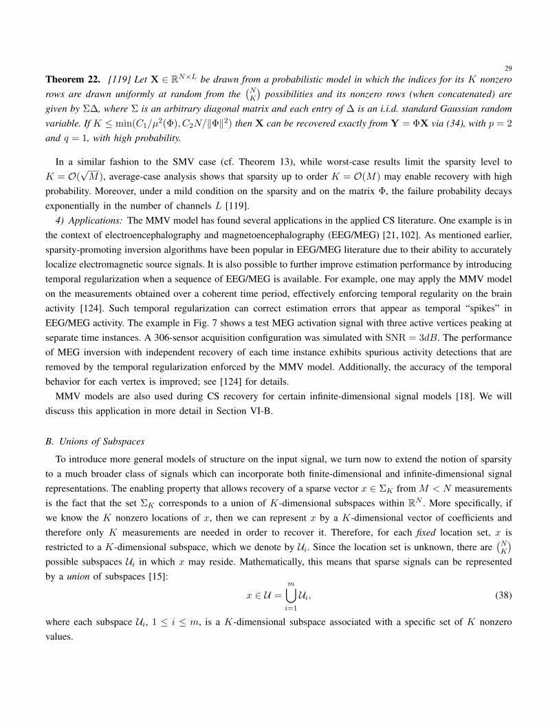
29

Theorem 22. [119] Let X ∈ RN×L be drawn from a probabilistic model in which the indices for its K nonzerorows are drawn uniformly at random from the

(NK

)possibilities and its nonzero rows (when concatenated) are

given by Σ∆, where Σ is an arbitrary diagonal matrix and each entry of ∆ is an i.i.d. standard Gaussian randomvariable. If K ≤ min(C1/µ

2(Φ), C2N/‖Φ‖2) then X can be recovered exactly from Y = ΦX via (34), with p = 2

and q = 1, with high probability.

In a similar fashion to the SMV case (cf. Theorem 13), while worst-case results limit the sparsity level toK = O(

√M), average-case analysis shows that sparsity up to order K = O(M) may enable recovery with high

probability. Moreover, under a mild condition on the sparsity and on the matrix Φ, the failure probability decaysexponentially in the number of channels L [119].

4) Applications: The MMV model has found several applications in the applied CS literature. One example is inthe context of electroencephalography and magnetoencephalography (EEG/MEG) [21, 102]. As mentioned earlier,sparsity-promoting inversion algorithms have been popular in EEG/MEG literature due to their ability to accuratelylocalize electromagnetic source signals. It is also possible to further improve estimation performance by introducingtemporal regularization when a sequence of EEG/MEG is available. For example, one may apply the MMV modelon the measurements obtained over a coherent time period, effectively enforcing temporal regularity on the brainactivity [124]. Such temporal regularization can correct estimation errors that appear as temporal “spikes” inEEG/MEG activity. The example in Fig. 7 shows a test MEG activation signal with three active vertices peaking atseparate time instances. A 306-sensor acquisition configuration was simulated with SNR = 3dB. The performanceof MEG inversion with independent recovery of each time instance exhibits spurious activity detections that areremoved by the temporal regularization enforced by the MMV model. Additionally, the accuracy of the temporalbehavior for each vertex is improved; see [124] for details.

MMV models are also used during CS recovery for certain infinite-dimensional signal models [18]. We willdiscuss this application in more detail in Section VI-B.

B. Unions of Subspaces

To introduce more general models of structure on the input signal, we turn now to extend the notion of sparsityto a much broader class of signals which can incorporate both finite-dimensional and infinite-dimensional signalrepresentations. The enabling property that allows recovery of a sparse vector x ∈ ΣK from M < N measurementsis the fact that the set ΣK corresponds to a union of K-dimensional subspaces within RN . More specifically, ifwe know the K nonzero locations of x, then we can represent x by a K-dimensional vector of coefficients andtherefore only K measurements are needed in order to recover it. Therefore, for each fixed location set, x isrestricted to a K-dimensional subspace, which we denote by Ui. Since the location set is unknown, there are

(NK

)

possible subspaces Ui in which x may reside. Mathematically, this means that sparse signals can be representedby a union of subspaces [15]:

x ∈ U =

m⋃

i=1

Ui, (38)

where each subspace Ui, 1 ≤ i ≤ m, is a K-dimensional subspace associated with a specific set of K nonzerovalues.

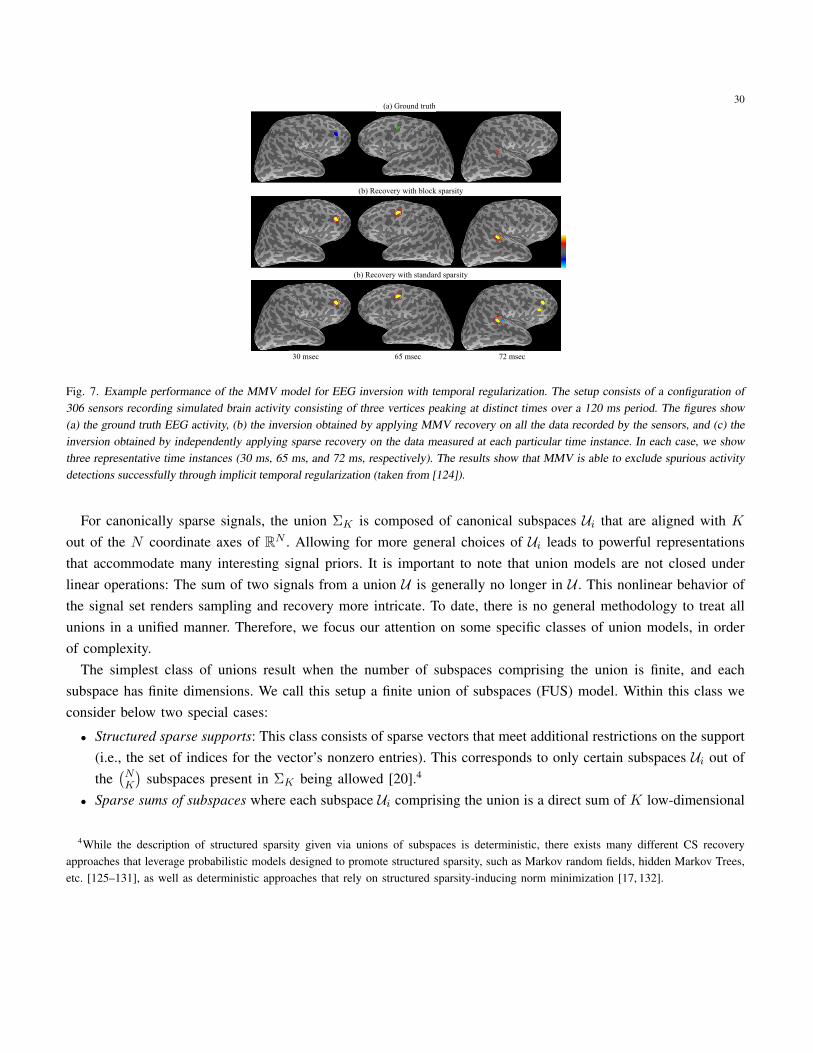
30(a) Ground truth

(b) Recovery with block sparsity

(b) Recovery with standard sparsity

30 msec 65 msec 72 msec

Fig. 7. Example performance of the MMV model for EEG inversion with temporal regularization. The setup consists of a configuration of306 sensors recording simulated brain activity consisting of three vertices peaking at distinct times over a 120 ms period. The figures show(a) the ground truth EEG activity, (b) the inversion obtained by applying MMV recovery on all the data recorded by the sensors, and (c) theinversion obtained by independently applying sparse recovery on the data measured at each particular time instance. In each case, we showthree representative time instances (30 ms, 65 ms, and 72 ms, respectively). The results show that MMV is able to exclude spurious activitydetections successfully through implicit temporal regularization (taken from [124]).

For canonically sparse signals, the union ΣK is composed of canonical subspaces Ui that are aligned with K

out of the N coordinate axes of RN . Allowing for more general choices of Ui leads to powerful representationsthat accommodate many interesting signal priors. It is important to note that union models are not closed underlinear operations: The sum of two signals from a union U is generally no longer in U . This nonlinear behavior ofthe signal set renders sampling and recovery more intricate. To date, there is no general methodology to treat allunions in a unified manner. Therefore, we focus our attention on some specific classes of union models, in orderof complexity.

The simplest class of unions result when the number of subspaces comprising the union is finite, and eachsubspace has finite dimensions. We call this setup a finite union of subspaces (FUS) model. Within this class weconsider below two special cases:

• Structured sparse supports: This class consists of sparse vectors that meet additional restrictions on the support(i.e., the set of indices for the vector’s nonzero entries). This corresponds to only certain subspaces Ui out ofthe(NK

)subspaces present in ΣK being allowed [20].4

• Sparse sums of subspaces where each subspace Ui comprising the union is a direct sum of K low-dimensional

4While the description of structured sparsity given via unions of subspaces is deterministic, there exists many different CS recoveryapproaches that leverage probabilistic models designed to promote structured sparsity, such as Markov random fields, hidden Markov Trees,etc. [125–131], as well as deterministic approaches that rely on structured sparsity-inducing norm minimization [17, 132].

31

subspaces [17]Ui =

⊕

|j|=KAj . (39)

Here Aj , 1 ≤ j ≤ m are a given set of subspaces with dimensions dim(Aj) = dj , and |j| = K denotesa sum over K indices. Thus, each subspace Ui corresponds to a different choice of K subspaces Aj thatcomprise the sum. The dimensionality of the signal representation in this case will be N =

∑mj=1 dj ; for

simplicity, we will often let dj = d for all j so that N = dm. As we show, this model leads to block sparsityin which certain blocks in a vector are zero, and others are not [120, 133, 134]. This framework can modelstandard sparsity by letting Aj , j = 1, . . . , N be the one-dimensional subspace spanned by the jth canonicalvector.

The two FUS cases above can be combined to allow only certain sums of K subspaces to be part of the union U .More complicated is the setting in which the number of possibilities is still finite while each underlying subspace

has infinite dimensions. Finally, there may be infinitely many possibilities of finite or infinite subspaces. Theselast two classes allow us to treat different families of analog signals, and will be considered in more detail inSection VI.

1) Conditions on measurement matrices: Guarantees for signal recovery using a FUS model can be developedby extending tools used in the standard sparse setting. For example, the (U , δ)-RIP for FUS models [15–17, 20]is similar to the standard RIP where instead of the inequalities in (7) having to be satisfied for all sparse vectorsx ∈ ΣK , they have to hold only for vectors x ∈ U . If the constant δ is small enough, then it can be shown thatrecovery algorithms tailored to the FUS model will recover the true underlying vector x.

An important question is how many samples are needed roughly in order to guarantee stable recovery. Thisquestion is addressed in the following proposition [16, 17, 20, 46].

Proposition 1 ([46, Theorem 3.3]). Consider a matrix Φ of size M ×N with entries independently drawn froma subgaussian distribution, and let U be composed of L subspaces of dimension D. Let t > 0 and 0 < δ < 1 beconstant numbers. If

M ≥ 36

7δ

(ln(L) +D ln

(12

δ

)+ t

), (40)

then Φ satisfies the (U , δ)-RIP with probability at least 1− e−t.

As observed in [46], the first term in (40) has the dominant impact on the required number of measurements forsparse signals in an asymptotic sense. This term quantifies the amount of measurements that are needed to codethe exact subspace where the sparse signal resides. We now specialize this result to the two FUS classes givenearlier.

• In the structured sparse supports case, L corresponds to the number of distinct K-sparse supports allowed bythe constraints, with L ≤

(NK

); this implies a reduction in the number of measurements needed as compared

to the traditional sparsity model. Additionally, D = K, since each subspace has dimension K.• For the sparse sum of subspaces setting, we focus on the case where each Aj is of dimension d; we then

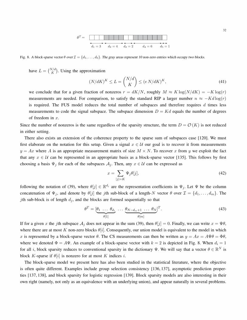
32

=

d1 = 3 d4 = 6d2 = 4 d5 = 1d2 = 2

Fig. 8. A block-sparse vector θ over I = d1, . . . , d5. The gray areas represent 10 non-zero entries which occupy two blocks.

have L =(N/dK

). Using the approximation

(N/dK)K ≤ L =

(N/d

K

)≤ (eN/dK)K , (41)

we conclude that for a given fraction of nonzeros r = dK/N , roughly M ≈ K log(N/dK) = −K log(r)

measurements are needed. For comparison, to satisfy the standard RIP a larger number n ≈ −Kd log(r)

is required. The FUS model reduces the total number of subspaces and therefore requires d times lessmeasurements to code the signal subspace. The subspace dimension D = Kd equals the number of degreesof freedom in x.

Since the number of nonzeros is the same regardless of the sparsity structure, the term D = O (K) is not reducedin either setting.

There also exists an extension of the coherence property to the sparse sum of subspaces case [120]. We mustfirst elaborate on the notation for this setup. Given a signal x ∈ U our goal is to recover it from measurementsy = Ax where A is an appropriate measurement matrix of size M ×N . To recover x from y we exploit the factthat any x ∈ U can be represented in an appropriate basis as a block-sparse vector [135]. This follows by firstchoosing a basis Ψj for each of the subspaces Aj . Then, any x ∈ U can be expressed as

x =∑

|j|=KΨjθ[j], (42)

following the notation of (39), where θ[j] ∈ Rdj are the representation coefficients in Ψj . Let Ψ be the columnconcatenation of Ψj , and denote by θ[j] the jth sub-block of a length-N vector θ over I = d1, . . . , dm. Thejth sub-block is of length dj , and the blocks are formed sequentially so that

θT = [θ1 . . . θd1︸ ︷︷ ︸θ[1]

. . . θN−dm+1 . . . θN︸ ︷︷ ︸θ[m]

]T . (43)

If for a given x the jth subspace Aj does not appear in the sum (39), then θ[j] = 0. Finally, we can write x = Ψθ,where there are at most K non-zero blocks θ[i]. Consequently, our union model is equivalent to the model in whichx is represented by a block-sparse vector θ. The CS measurements can then be written as y = Ax = AΨθ = Φθ,where we denoted Φ = AΨ. An example of a block-sparse vector with k = 2 is depicted in Fig. 8. When di = 1

for all i, block sparsity reduces to conventional sparsity in the dictionary Ψ. We will say that a vector θ ∈ RN isblock K-sparse if θ[i] is nonzero for at most K indices i.

The block-sparse model we present here has also been studied in the statistical literature, where the objectiveis often quite different. Examples include group selection consistency [136, 137], asymptotic prediction proper-ties [137, 138], and block sparsity for logistic regression [139]. Block sparsity models are also interesting in theirown right (namely, not only as an equivalence with an underlying union), and appear naturally in several problems.

33

Examples include DNA microarray analysis [140, 141], equalization of sparse communication channels [105], andsource localization [104].

We now introduce the adaptation of coherence to sparse sums of subspaces: the block-coherence of a matrix Φ

is defined asµB(Φ) = max

`,r 6=`1

dρ(ΦH [`]Φ[r]) (44)

with ρ(A) denoting the spectral norm of the matrix A. Here Φ is represented as a concatenation of column-blocksΦ[`] of size M × d:

Φ = [φ1 . . . φd︸ ︷︷ ︸Φ[1]

φd+1 . . . φ2d︸ ︷︷ ︸Φ[2]

. . . φN−d+1 . . . φN︸ ︷︷ ︸Φ[m]

]. (45)

When d = 1, as expected, µB(Φ) = µ(Φ). More generally, µB(Φ) ≤ µ(Φ).While µB(Φ) quantifies global properties of the matrix Φ, local properties are characterized by the sub-coherence

of Φ, defined as

ν(Φ) = max`

maxi,j 6=i|φHi φj |, φi, φj ∈ Φ[`]. (46)

We define ν(Φ) = 0 for d = 1. In addition, if the columns of Φ[`] are orthogonal for each `, then ν(Φ) = 0.2) Recovery algorithms: Like in the MMV setting, it is possible to extend standard sparsity-based signal

recovery algorithms to the FUS model. For example, greedy algorithms may be modified easily by changingthe thresholding T (x,K) (which finds the best approximation of x in the union of subspaces ΣK) to a structuredsparse approximation step:

MU (x) = arg minx′∈U‖x− x′‖2. (47)

For example, the CoSaMP algorithm (see Algorithm 2) is modified according to the FUS model [20] by changingthe following two steps:

• Prune residual: Ω← supp(MU2(e)).

• Prune signal: xi ←MU (b).

A similar change can be made to the IHT algorithm (15) to obtain a model-based IHT variant:

xi = MU (xi−1 + ΦT (y − Φxi−1)).

Structured sparse approximation algorithms of the form (47) are feasible and computationally efficient for a varietyof structured sparse support models [20, 142–144]. For example, the approximation algorithm MU under blocksparsity is equivalent to block thresholding, with the K blocks with the largest energies (or `2 norms) beingpreserved; we will show another example in greater detail later in this section.

For the sparse sum of subspaces setting, it is possible to formulate optimization-based algorithms for signalrecovery. A convex recovery method can be obtained by minimizing the sum of the energy of the blocks θ[i]. Towrite down the problem explicitly, we define the mixed `2/`1 norm as

‖θ‖2,I =

m∑

i=1

‖θ[i]‖2. (48)

34

We may then recover θ by solving [17, 134, 136, 137]

θ = arg minθ∈RN

‖θ‖2,I subject to y = Φθ. (49)

The optimization constraints can be relaxed to address the case of noisy measurements, in a way similar to thestandard BPIC algorithm. Generalizations of greedy algorithms to the block sparse setting have been developed in[101, 120].

3) Recovery guarantees: Many recovery methods for the FUS model inherit the guarantees of their standardcounterparts. Our first example deals with the model-based CoSaMP algorithm. Since CoSaMP requires RIP oforder 4K, here we must rely on enlarged unions of subspaces.

Definition 6. For an integer J and a FUS model U , denote the J-sum of U as the sum of subspaces

SJ(U) =⊕

|j|=JUj , (50)

following the notation of (39), which contains all sums of J signals belonging in U .

We can then pose the following guarantee.Theorem 23. [20] Let x ∈ U and let y = Φx+n be a set of noisy CS measurements. If Φ has the (S4(U), δ)-RIPwith δ ≤ 0.1, then the signal estimate xi obtained from iteration i of the model-based CoSaMP algorithm satisfies

‖x− xi‖2 ≤ 2−i‖x‖2 + 15‖n‖2. (51)

One can also show that under an additional condition on Φ the algorithm is stable to signal mismodeling [20].Similar guarantees exist for the model-based IHT algorithm [20].

Guarantees are also available for the optimization-based approach used in the sparse sum of subspaces setting.Theorem 24. [17] Let x ∈ RN and let y = Φx + n be a set of noisy CS measurements, with ‖n‖2 ≤ ε. If Φ

has the (S2(U), δ)-RIP with δ ≤√

2 − 1, then the signal estimate x obtained from (49) with relaxed constraints‖y − Φx‖2 ≤ ε satisfies

‖x− x‖2 ≤ C1K−1/2‖x−MU (x)‖2 + C2ε, (52)

where MU (x) is defined in (47), and U is a sparse sum of subspaces.

Finally, we point out that recovery guarantees can also be obtained based on block coherence.Theorem 25. [120] Both the greedy methods and the optimization-based approach of (49) recover a block-sparsevector θ from measurements y = Φθ if the block-coherence satisfies

Kd <1

2

(1

µB(Φ)+ d− (d− 1)

ν(Φ)

µB(Φ)

). (53)

In the special case in which the columns of Φ[`] are orthonormal for each `, we have ν(Φ) = 0 and therefore therecovery condition becomes Kd < (µ−1

B (Φ) + d)/2. Comparing to Theorem 4 for recovery of a conventional Kd-sparse signal we can see that, thanks to µB(Φ) ≤ µ(Φ), making explicit use of block-sparsity leads to guaranteedrecovery for a potentially higher sparsity level. These results can also be extended to both adversarial and randomadditive noise in the measurements [145].

35

...

(a) (b) (c)

Fig. 9. The class of tree-sparse signals is an example of a FUS that enforces structure in the sparse signal support. (a) Example of a tree-structured sparse support for a 1-D piecewise smooth signal’s wavelet coefficients (taken from [20]). (b) Example recovery of the N =

512 × 512 = 262144-pixel Peppers test image from M = 40000 random measurements (15%) using standard CoSaMP (SNR =17.45dB).(c) Example recovery of the same image from the same measurements using model-based CoSaMP for the tree-structured FUS model (SNR =22.6dB). In both cases, the Daubechies-8 wavelet basis was used as the sparsity/compressibility transform.

4) Applications: A particularly interesting example of structured sparse supports corresponds to tree-structuredsupports [20]. For signals that are smooth or piecewise smooth, including natural images, sufficiently smoothwavelet bases provide sparse or compressible representations θ. Additionally, because each wavelet basis elementacts as a discontinuity detector in a local region of the signal at a certain scale, it is possible to link together waveletbasis elements corresponding to a given location at neighboring scales, forming what are known as branches thatconnect at the coarsest wavelet scale. The corresponding full graph is known as a wavelet tree. For locations wherethere exist discontinuities, the corresponding branches of wavelet coefficients tend to be large, forming a connectedsubtree inside the wavelet tree. Thus, the restriction of U ⊆ ΣK includes only the subspaces corresponding to thistype of structure in the signal’s support. Figure 9(a) shows an example of a tree-sparse 1-D signal support for awavelet coefficient vector. Since the number of possible supports containing this structure is limited to L ≤ CK/Kfor a constant C, we obtain that M = O (K) random measurements are needed to recover these signals usingmodel-based recovery algorithms. Additionally, there exist approximation algorithms to implement M for this FUSmodel based on both greedy and optimization-based approaches; see [20] for more details. Figure 9(b) shows anexample of improved signal recovery from random measurements leveraging the FUS model.

In our development so far, we did not consider any structure within the subspaces comprising the unions.In certain applications it may be beneficial to add internal structure. For example, the coefficient vectors θ[j]may themselves be sparse. Such scenarios can be accounted for by adding an `1 penalty in (49) on the individualblocks [146], an approach that is dubbed C-HiLasso in [147]. This allows to combine the sparsity-inducing propertyof `1 optimization at the individual feature level, with the block-sparsity property of (49) on the group level,obtaining a hierarchically structured sparsity pattern. An example FUS model featuring sparse sums of subspacesthat exploits the additional structure described above is shown in Fig. 10. This example is based on identification

36

Fig. 10. Example of recovered digits (3 and 5) from a mixture with 60% of missing components. From left to right: noiseless mixture, observedmixture with missing pixels highlighted in red, recovered digits 3 and 5, and active set recovered for 180 different mixtures using the C-HiLassoand (13) respectively. The last two figures show the active sets of the recovered coefficients vectors θ as a matrix (one column per mixture),where black dots indicate nonzero coefficients. The coefficients corresponding to the subspace bases for digits 3 and 5 are marked as pink bands.Notice that C-HiLasso efficiently exploits the FUS model, succeeding in recovering the correct active groups in all the samples. The standardapproach (13), which lacks this stronger signal model, clearly is not capable of doing so, and active sets spread all over the groups (takenfrom [147]).

of digits; a separate subspace is trained for each digit 0, . . . , 9, and the task addressed is separation of a mixtureof digits from subsampled information. We collect bases that span each of the 10 subspaces A0, . . . ,A9 into adictionary Φ, and apply the FUS model where the subspaces Ui considered correspond to mixtures of pairs ofdigits. The FUS model allows for successful source identification and separation.

VI. STRUCTURE IN INFINITE-DIMENSIONAL MODELS

One of the prime goals of CS is to allow for reduced-rate sampling of analog signals. In fact, many of theoriginal papers in the field state this as a motivating drive for the theory of CS. In this section we focus onunion models that include a degree of infiniteness: This can come into play either by allowing for infinitely manysubspaces, by letting the subspaces have infinite dimension, or both. As we will show, the resulting models maybe used to describe a broad class of structured continuous-time signals. We will then demonstrate how such priorscan be translated into concrete hardware solutions that allow sampling and recovery of analog signals at rates farbelow that dictated by Nyquist.

The approach we present here to reduced-rate sampling is based on viewing analog signals in unions of subspaces,and is therefore fundamentally different than previous attempts to treat similar problems, [42, 84, 104, 148, 149].The latter typically rely on discretization of the analog input, and are often not concerned with the actual hardware.Furthermore, in some cases the reduced rate analog stage results in high rate DSP. In contrast, in all of the examplesbelow we treat the analog formulation directly, the DSP can be performed in real time at the low rate, and the analogfront end can be implemented in hardware using standard analog design components such as modulators, low rateanalog-to-digital converters (ADCs) and low-pass filters (LPFs). A more detailed discussion on the comparison todiscretized approaches can be found in [10, 150].

In our review, we consider three main cases:

• finite unions of infinite dimensional spaces;• infinite unions of finite dimensional spaces;• infinite unions of infinite dimensional spaces.

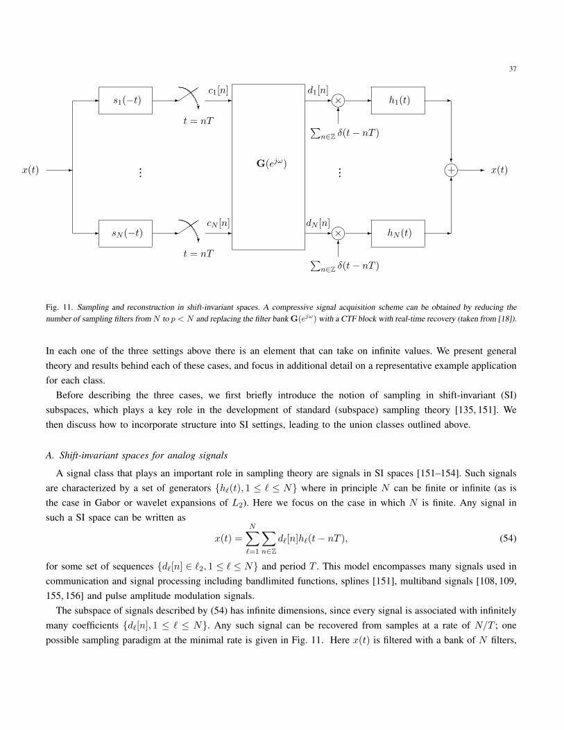
37

- sN (−t) -

?

t = nT

- - m× - hN (t) -cN [n]

∑n∈Z δ(t− nT )

6

dN [n]

... ...

- s1(−t) -

?

t = nT

- - m× - h1(t) -c1[n]

∑n∈Z δ(t− nT )

6

d1[n]

x(t) - G(ejω) m - x(t)

6

?

Fig. 11. Sampling and reconstruction in shift-invariant spaces. A compressive signal acquisition scheme can be obtained by reducing thenumber of sampling filters from N to p < N and replacing the filter bank G(ejω) with a CTF block with real-time recovery (taken from [18]).

In each one of the three settings above there is an element that can take on infinite values. We present generaltheory and results behind each of these cases, and focus in additional detail on a representative example applicationfor each class.

Before describing the three cases, we first briefly introduce the notion of sampling in shift-invariant (SI)subspaces, which plays a key role in the development of standard (subspace) sampling theory [135, 151]. Wethen discuss how to incorporate structure into SI settings, leading to the union classes outlined above.

A. Shift-invariant spaces for analog signals

A signal class that plays an important role in sampling theory are signals in SI spaces [151–154]. Such signalsare characterized by a set of generators h`(t), 1 ≤ ` ≤ N where in principle N can be finite or infinite (as isthe case in Gabor or wavelet expansions of L2). Here we focus on the case in which N is finite. Any signal insuch a SI space can be written as

x(t) =

N∑

`=1

∑

n∈Zd`[n]h`(t− nT ), (54)

for some set of sequences d`[n] ∈ `2, 1 ≤ ` ≤ N and period T . This model encompasses many signals used incommunication and signal processing including bandlimited functions, splines [151], multiband signals [108, 109,155, 156] and pulse amplitude modulation signals.

The subspace of signals described by (54) has infinite dimensions, since every signal is associated with infinitelymany coefficients d`[n], 1 ≤ ` ≤ N. Any such signal can be recovered from samples at a rate of N/T ; onepossible sampling paradigm at the minimal rate is given in Fig. 11. Here x(t) is filtered with a bank of N filters,

38

each with impulse response s`(t) which can be almost arbitrary, and the outputs are uniformly sampled with periodT . Denote by c(ω) a vector collecting the frequency responses of c`[n], 1 ≤ ` ≤ N . The signal is then recoveredby first processing the samples with a filter bank with frequency response G(ejω), which depends on the samplingfilters and the generators h`(t) (see [18] for details). In this way we obtain the vectors

d(ω) = G(ejω)c(ω) (55)

containing the frequency responses of the sequences d`[n], 1 ≤ ` ≤ N . Each output sequence is then modulatedby a periodic impulse train

∑n∈Z δ(t − nT ) with period T , followed by filtering with the corresponding analog

filter h`(t).In the ensuing subsections we consider settings in which further structure is incorporated into the generic SI

model (54). In Sections VI-B and VI-D we treat signals of the form (54) involving a small number K of generators,chosen from a finite or infinite set, respectively, while in Section VI-C we consider a finite-dimensional counterpartof (54) in which the generators are chosen from an infinite set. All of these examples lead to union of subspacesmodels for analog signals. Our goal is to exploit the available structure in order to reduce the sampling rate.

Before presenting the more detailed applications we point out that in all the examples below the philosophyis similar: we develop an analog sensing stage that consists of simple hardware devices designed to spread out(alias) the signal prior to sampling, in such a way that the samples contain energy from all subspace components.The first step in the digital reconstruction stage identifies the underlying subspace structure. Recovery is thenperformed in a subspace once the parameters defining the subspace are determined. The difference between theexamples is in how the aliasing is obtained and in the digital recovery step which identifies the subspace. Thisframework has been dubbed Xampling in [9, 10], which combines CS and sampling, emphasizing that this is ananalog counterpart to discrete CS theory and methods.

B. Finite union of infinite-dimensional subspaces

In this first case, we follow the model (38-39) where U is composed of a finite number m of subspaces, andeach subspace has infinite dimension (i.e., dj =∞ for 1 ≤ j ≤ m).

1) Analog signal model: To incorporate structure into (54) we proceed in two ways (see Section VI-D for thecomplement). In the first, we assume that only K of the N generators are active, leading to the model

x(t) =∑

|`|=K

∑

n∈Zd`[n]h`(t− nT ), (56)

where the notation |`| = K means a union (or sum) over at most K elements. If the K active generators are known,then it suffices to sample at a rate of K/T corresponding to uniform samples with period T at the output of Kappropriate filters. However, a more difficult question is whether the rate can be reduced if we know that only Kof the generators are active, but do not know in advance which ones. This is a special case of the model (39) wherenow each of the subspaces A` is a single-generator SI subspace spanned by h`(t). For this model, it is possible toreduce the sampling rate to as low as 2K/T [18]. Such rate reduction is achieved by using a bank of appropriatesampling filters that replaces the filters s`(t) in Fig. 11, followed by postprocessing via subspace reduction andsolving an MMV problem (cf. Section V-A). We now describe the main ideas underlying this approach.

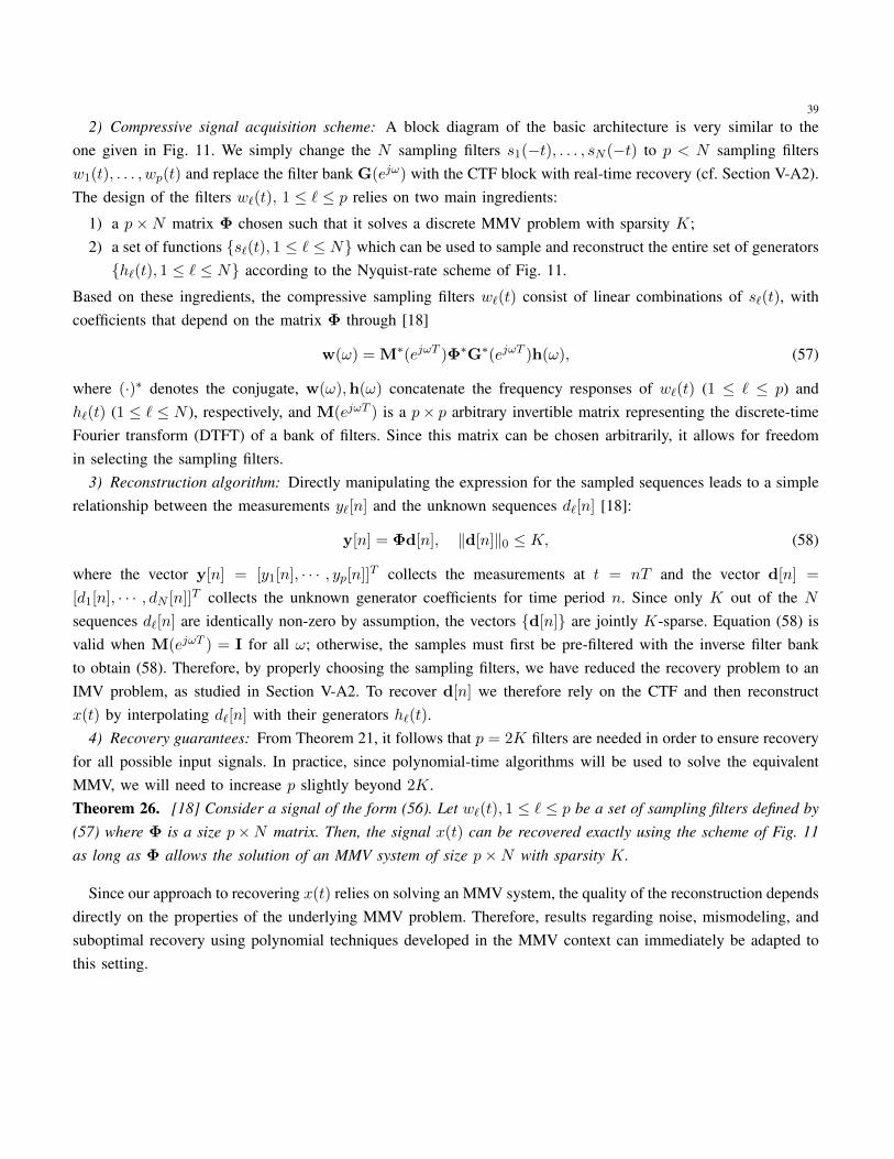
39

2) Compressive signal acquisition scheme: A block diagram of the basic architecture is very similar to theone given in Fig. 11. We simply change the N sampling filters s1(−t), . . . , sN (−t) to p < N sampling filtersw1(t), . . . , wp(t) and replace the filter bank G(ejω) with the CTF block with real-time recovery (cf. Section V-A2).The design of the filters w`(t), 1 ≤ ` ≤ p relies on two main ingredients:

1) a p×N matrix Φ chosen such that it solves a discrete MMV problem with sparsity K;2) a set of functions s`(t), 1 ≤ ` ≤ N which can be used to sample and reconstruct the entire set of generatorsh`(t), 1 ≤ ` ≤ N according to the Nyquist-rate scheme of Fig. 11.

Based on these ingredients, the compressive sampling filters w`(t) consist of linear combinations of s`(t), withcoefficients that depend on the matrix Φ through [18]

w(ω) = M∗(ejωT )Φ∗G∗(ejωT )h(ω), (57)

where (·)∗ denotes the conjugate, w(ω),h(ω) concatenate the frequency responses of w`(t) (1 ≤ ` ≤ p) andh`(t) (1 ≤ ` ≤ N ), respectively, and M(ejωT ) is a p× p arbitrary invertible matrix representing the discrete-timeFourier transform (DTFT) of a bank of filters. Since this matrix can be chosen arbitrarily, it allows for freedomin selecting the sampling filters.

3) Reconstruction algorithm: Directly manipulating the expression for the sampled sequences leads to a simplerelationship between the measurements y`[n] and the unknown sequences d`[n] [18]:

y[n] = Φd[n], ‖d[n]‖0 ≤ K, (58)

where the vector y[n] = [y1[n], · · · , yp[n]]T collects the measurements at t = nT and the vector d[n] =

[d1[n], · · · , dN [n]]T collects the unknown generator coefficients for time period n. Since only K out of the Nsequences d`[n] are identically non-zero by assumption, the vectors d[n] are jointly K-sparse. Equation (58) isvalid when M(ejωT ) = I for all ω; otherwise, the samples must first be pre-filtered with the inverse filter bankto obtain (58). Therefore, by properly choosing the sampling filters, we have reduced the recovery problem to anIMV problem, as studied in Section V-A2. To recover d[n] we therefore rely on the CTF and then reconstructx(t) by interpolating d`[n] with their generators h`(t).

4) Recovery guarantees: From Theorem 21, it follows that p = 2K filters are needed in order to ensure recoveryfor all possible input signals. In practice, since polynomial-time algorithms will be used to solve the equivalentMMV, we will need to increase p slightly beyond 2K.Theorem 26. [18] Consider a signal of the form (56). Let w`(t), 1 ≤ ` ≤ p be a set of sampling filters defined by(57) where Φ is a size p×N matrix. Then, the signal x(t) can be recovered exactly using the scheme of Fig. 11as long as Φ allows the solution of an MMV system of size p×N with sparsity K.

Since our approach to recovering x(t) relies on solving an MMV system, the quality of the reconstruction dependsdirectly on the properties of the underlying MMV problem. Therefore, results regarding noise, mismodeling, andsuboptimal recovery using polynomial techniques developed in the MMV context can immediately be adapted tothis setting.

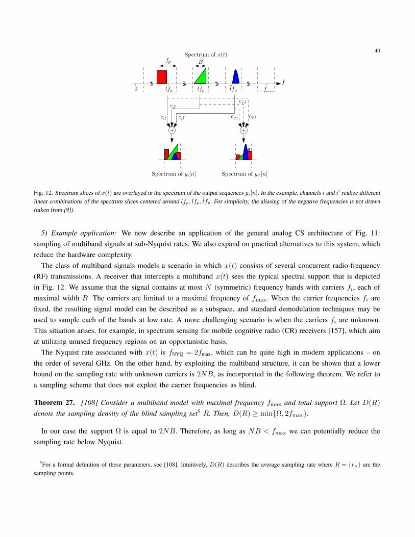
40

f0

maxf

fp

lfp lfp lfp

+

cil

cil

cil

Spectrum of x(t)

Spectrum of yi[n] Spectrum of yi′ [n]

+

ci′l

ci′ l

ci′ l

B

Fig. 12. Spectrum slices of x(t) are overlayed in the spectrum of the output sequences yi[n]. In the example, channels i and i′ realize differentlinear combinations of the spectrum slices centered around lfp, lfp, lfp. For simplicity, the aliasing of the negative frequencies is not drawn(taken from [9]).

5) Example application: We now describe an application of the general analog CS architecture of Fig. 11:sampling of multiband signals at sub-Nyquist rates. We also expand on practical alternatives to this system, whichreduce the hardware complexity.

The class of multiband signals models a scenario in which x(t) consists of several concurrent radio-frequency(RF) transmissions. A receiver that intercepts a multiband x(t) sees the typical spectral support that is depictedin Fig. 12. We assume that the signal contains at most N (symmetric) frequency bands with carriers fi, each ofmaximal width B. The carriers are limited to a maximal frequency of fmax. When the carrier frequencies fi arefixed, the resulting signal model can be described as a subspace, and standard demodulation techniques may beused to sample each of the bands at low rate. A more challenging scenario is when the carriers fi are unknown.This situation arises, for example, in spectrum sensing for mobile cognitive radio (CR) receivers [157], which aimat utilizing unused frequency regions on an opportunistic basis.

The Nyquist rate associated with x(t) is fNYQ = 2fmax, which can be quite high in modern applications – onthe order of several GHz. On the other hand, by exploiting the multiband structure, it can be shown that a lowerbound on the sampling rate with unknown carriers is 2NB, as incorporated in the following theorem. We refer toa sampling scheme that does not exploit the carrier frequencies as blind.

Theorem 27. [108] Consider a multiband model with maximal frequency fmax and total support Ω. Let D(R)

denote the sampling density of the blind sampling set5 R. Then, D(R) ≥ minΩ, 2fmax.

In our case the support Ω is equal to 2NB. Therefore, as long as NB < fmax we can potentially reduce thesampling rate below Nyquist.

5For a formal definition of these parameters, see [108]. Intuitively, D(R) describes the average sampling rate where R = rn are thesampling points.

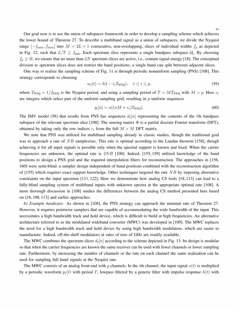
41

Our goal now is to use the union of subspaces framework in order to develop a sampling scheme which achievesthe lower bound of Theorem 27. To describe a multiband signal as a union of subspaces, we divide the Nyquistrange [−fmax, fmax] into M = 2L + 1 consecutive, non-overlapping, slices of individual widths fp as depictedin Fig. 12, such that L/T ≥ fmax. Each spectrum slice represents a single bandpass subspace Ui. By choosingfp ≥ B, we ensure that no more than 2N spectrum slices are active, i.e., contain signal energy [18]. The conceptualdivision to spectrum slices does not restrict the band positions; a single band can split between adjacent slices.

One way to realize the sampling scheme of Fig. 11 is through periodic nonuniform sampling (PNS) [108]. Thisstrategy corresponds to choosing

wi(t) = δ(t− ciTNYQ), 1 ≤ i ≤ p, (59)

where TNYQ = 1/fNYQ is the Nyquist period, and using a sampling period of T = MTNYQ with M > p. Here ciare integers which select part of the uniform sampling grid, resulting in p uniform sequences

yi[n] = x((nM + ci)TNYQ). (60)

The IMV model (58) that results from PNS has sequences d`[n] representing the contents of the `th bandpasssubspace of the relevant spectrum slice [108]. The sensing matrix Φ is a partial discrete Fourier transform (DFT),obtained by taking only the row indices ci from the full M ×M DFT matrix.

We note that PNS was utilized for multiband sampling already in classic studies, though the traditional goalwas to approach a rate of NB samples/sec. This rate is optimal according to the Landau theorem [158], thoughachieving it for all input signals is possible only when the spectral support is known and fixed. When the carrierfrequencies are unknown, the optimal rate is 2NB [108]. Indeed, [155, 159] utilized knowledge of the bandpositions to design a PNS grid and the required interpolation filters for reconstruction. The approaches in [156,160] were semi-blind: a sampler design independent of band positions combined with the reconstruction algorithmof [155] which requires exact support knowledge. Other techniques targeted the rate NB by imposing alternativeconstraints on the input spectrum [111, 122]. Here we demonstrate how analog CS tools [18, 113] can lead to afully-blind sampling system of multiband inputs with unknown spectra at the appropriate optimal rate [108]. Amore thorough discussion in [108] studies the differences between the analog CS method presented here basedon [18, 108, 113] and earlier approaches.

6) Example hardware: As shown in [108], the PNS strategy can approach the minimal rate of Theorem 27.However, it requires pointwise samplers that are capable of accommodating the wide bandwidth of the input. Thisnecessitates a high bandwidth track and hold device, which is difficult to build at high frequencies. An alternativearchitecture referred to as the modulated wideband converter (MWC) was developed in [109]. The MWC replacesthe need for a high bandwidth track and hold device by using high bandwidth modulators, which are easier tomanufacture. Indeed, off-the-shelf modulators at rates of tens of GHz are readily available.

The MWC combines the spectrum slices d`[n] according to the scheme depicted in Fig. 13. Its design is modularso that when the carrier frequencies are known the same receiver can be used with fewer channels or lower samplingrate. Furthermore, by increasing the number of channels or the rate on each channel the same realization can beused for sampling full band signals at the Nyquist rate.

The MWC consists of an analog front-end with p channels. In the ith channel, the input signal x(t) is multipliedby a periodic waveform pi(t) with period T , lowpass filtered by a generic filter with impulse response h(t) with

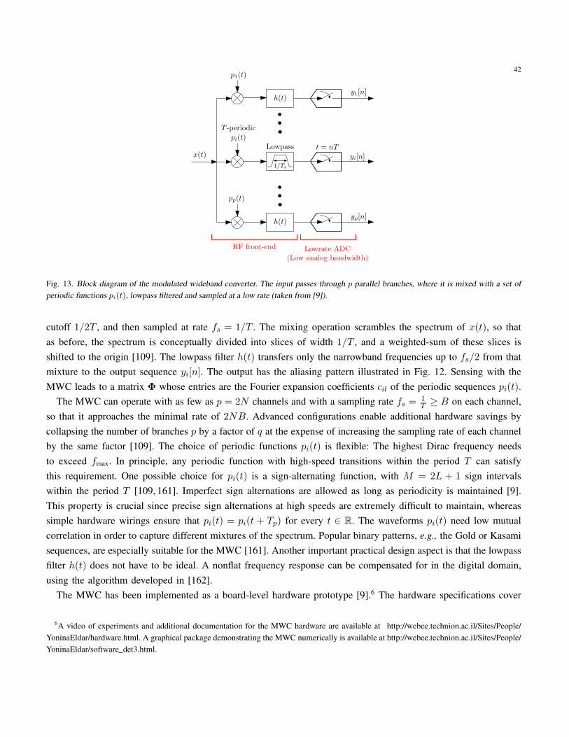
42

yi[n]

h(t)

p1(t)

h(t)

pp(t)

x(t)

yp[n]

y1[n]

Lowpass t = nT

T -periodic

1/Ts

pi(t)

RF front-end Lowrate ADC(Low analog bandwidth)

Fig. 13. Block diagram of the modulated wideband converter. The input passes through p parallel branches, where it is mixed with a set ofperiodic functions pi(t), lowpass filtered and sampled at a low rate (taken from [9]).

cutoff 1/2T , and then sampled at rate fs = 1/T . The mixing operation scrambles the spectrum of x(t), so thatas before, the spectrum is conceptually divided into slices of width 1/T , and a weighted-sum of these slices isshifted to the origin [109]. The lowpass filter h(t) transfers only the narrowband frequencies up to fs/2 from thatmixture to the output sequence yi[n]. The output has the aliasing pattern illustrated in Fig. 12. Sensing with theMWC leads to a matrix Φ whose entries are the Fourier expansion coefficients cil of the periodic sequences pi(t).

The MWC can operate with as few as p = 2N channels and with a sampling rate fs = 1T ≥ B on each channel,

so that it approaches the minimal rate of 2NB. Advanced configurations enable additional hardware savings bycollapsing the number of branches p by a factor of q at the expense of increasing the sampling rate of each channelby the same factor [109]. The choice of periodic functions pi(t) is flexible: The highest Dirac frequency needsto exceed fmax. In principle, any periodic function with high-speed transitions within the period T can satisfythis requirement. One possible choice for pi(t) is a sign-alternating function, with M = 2L + 1 sign intervalswithin the period T [109, 161]. Imperfect sign alternations are allowed as long as periodicity is maintained [9].This property is crucial since precise sign alternations at high speeds are extremely difficult to maintain, whereassimple hardware wirings ensure that pi(t) = pi(t + Tp) for every t ∈ R. The waveforms pi(t) need low mutualcorrelation in order to capture different mixtures of the spectrum. Popular binary patterns, e.g., the Gold or Kasamisequences, are especially suitable for the MWC [161]. Another important practical design aspect is that the lowpassfilter h(t) does not have to be ideal. A nonflat frequency response can be compensated for in the digital domain,using the algorithm developed in [162].

The MWC has been implemented as a board-level hardware prototype [9].6 The hardware specifications cover

6A video of experiments and additional documentation for the MWC hardware are available at http://webee.technion.ac.il/Sites/People/YoninaEldar/hardware.html. A graphical package demonstrating the MWC numerically is available at http://webee.technion.ac.il/Sites/People/YoninaEldar/software det3.html.

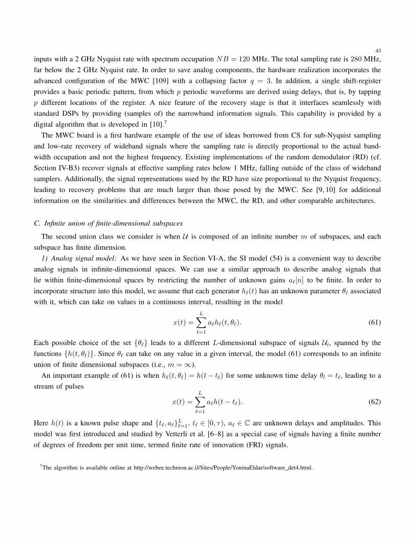
43

inputs with a 2 GHz Nyquist rate with spectrum occupation NB = 120 MHz. The total sampling rate is 280 MHz,far below the 2 GHz Nyquist rate. In order to save analog components, the hardware realization incorporates theadvanced configuration of the MWC [109] with a collapsing factor q = 3. In addition, a single shift-registerprovides a basic periodic pattern, from which p periodic waveforms are derived using delays, that is, by tappingp different locations of the register. A nice feature of the recovery stage is that it interfaces seamlessly withstandard DSPs by providing (samples of) the narrowband information signals. This capability is provided by adigital algorithm that is developed in [10].7

The MWC board is a first hardware example of the use of ideas borrowed from CS for sub-Nyquist samplingand low-rate recovery of wideband signals where the sampling rate is directly proportional to the actual band-width occupation and not the highest frequency. Existing implementations of the random demodulator (RD) (cf.Section IV-B3) recover signals at effective sampling rates below 1 MHz, falling outside of the class of widebandsamplers. Additionally, the signal representations used by the RD have size proportional to the Nyquist frequency,leading to recovery problems that are much larger than those posed by the MWC. See [9, 10] for additionalinformation on the similarities and differences between the MWC, the RD, and other comparable architectures.

C. Infinite union of finite-dimensional subspaces

The second union class we consider is when U is composed of an infinite number m of subspaces, and eachsubspace has finite dimension.

1) Analog signal model: As we have seen in Section VI-A, the SI model (54) is a convenient way to describeanalog signals in infinite-dimensional spaces. We can use a similar approach to describe analog signals thatlie within finite-dimensional spaces by restricting the number of unknown gains a`[n] to be finite. In order toincorporate structure into this model, we assume that each generator h`(t) has an unknown parameter θ` associatedwith it, which can take on values in a continuous interval, resulting in the model

x(t) =

L∑

`=1

a`h`(t, θ`). (61)

Each possible choice of the set θ` leads to a different L-dimensional subspace of signals Ui, spanned by thefunctions h(t, θ`). Since θ` can take on any value in a given interval, the model (61) corresponds to an infiniteunion of finite dimensional subspaces (i.e., m =∞).

An important example of (61) is when h`(t, θ`) = h(t− t`) for some unknown time delay θl = t`, leading to astream of pulses

x(t) =

L∑

`=1

a`h(t− t`). (62)

Here h(t) is a known pulse shape and t`, a`L`=1, t` ∈ [0, τ), a` ∈ C are unknown delays and amplitudes. Thismodel was first introduced and studied by Vetterli et al. [6–8] as a special case of signals having a finite numberof degrees of freedom per unit time, termed finite rate of innovation (FRI) signals.

7The algorithm is available online at http://webee.technion.ac.il/Sites/People/YoninaEldar/software det4.html.

44

Our goal is to sample x(t) and reconstruct it from a minimal number of samples. The primary interest is inpulses which have small time-support, and therefore the required Nyquist rate would be very high. However, sincethe pulse shape is known, the signal has only 2L degrees of freedom, and therefore, we expect the minimal numberof samples to be 2L, much lower than the number of samples resulting from Nyquist rate sampling.

A simpler version of the problem is when the signal x(t) of (62) is repeated periodically leading to the model

x(t) =∑

m∈Z

L∑

`=1

a`h(t− t` −mτ), (63)

where τ is the known period. This periodic setup is easier to treat because we can exploit the properties of theFourier series representation of x(t) due to the periodicity. The dimensionality and number of subspaces includedin the model (38) remain unchanged.

2) Compressive signal acquisition: To date, there are no general acquisition methods for signals of the form(61). Instead, we focus on the special case of (63).

Our sampling scheme follows the ideas of [6–8] and consists of a filter s(t) followed by uniform sampling ofthe output with period T = τ/N where N is the number of samples in one period, and N ≥ 2L. The resultingsamples can be written as inner products c[n] = 〈s(t− nT ), x(t)〉. The following theorem establishes propertiesof the filter s(t) that allow recovery from 2L samples.

Theorem 28. [163] Consider the τ -periodic stream of pulses of order L given by (63). Choose a set K ofconsecutive indices for which H(2πk/τ) 6= 0 where H(ω) is the Fourier transform of the pulse h(t). Then thesamples c[n] for n = 0, . . . , N − 1, uniquely determine the signal x(t) as long as N ≥ |K| ≥ 2L for any s(t)satisfying

S(ω) =

0 ω = 2πk/τ, k /∈ Knonzero ω = 2πk/τ, k ∈ Karbitrary otherwise.

(64)

Theorem 28 was initially focused on low pass filters in [6], and was later extended to arbitrary filters in [163].To see how we can recover x(t) from the samples of Theorem 28, we note that the Fourier series coefficients

X[k] of the periodic pulse stream x(t) are given by [6]:

X[k] =1

τH(2πk/τ)

L∑

`=1

a`e−j2πkt`/τ

=1

τH(2πk/τ)

L∑

`=1

a`uk` , (65)

where u` = e−j2πt`/τ . Given X[k], the problem of retrieving a` and t` in (65) is a standard problem in arrayprocessing [6, 164], and can be solved using methods developed in that context such as the matrix pencil [165],subspace-based estimators [166, 167], and the annihilating filter [8]. These methods require 2L Fourier coefficientsto determine a` and u`. In the next subsection, we show that the vector X of Fourier coefficients X[k] can becomputed from the N samples c[n] of Theorem 28.

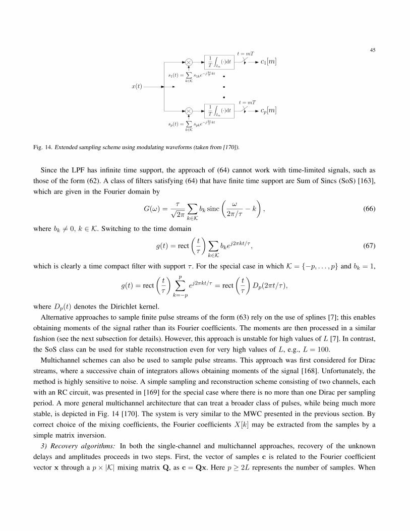
45

x(t)

1

T

!

Im

(·)dt c1[m]t = mT

cp[m]t = mT

s1(t) ="

k!Ks1ke

"j 2!T

kt

sp(t) ="

k!Kspke

"j 2!T

kt

1

T

!

Im

(·)dt

Fig. 14. Extended sampling scheme using modulating waveforms (taken from [170]).

Since the LPF has infinite time support, the approach of (64) cannot work with time-limited signals, such asthose of the form (62). A class of filters satisfying (64) that have finite time support are Sum of Sincs (SoS) [163],which are given in the Fourier domain by

G(ω) =τ√2π

∑

k∈Kbk sinc

(ω

2π/τ− k), (66)

where bk 6= 0, k ∈ K. Switching to the time domain

g(t) = rect(t

τ

)∑

k∈Kbke

j2πkt/τ , (67)

which is clearly a time compact filter with support τ . For the special case in which K = −p, . . . , p and bk = 1,

g(t) = rect(t

τ

) p∑

k=−pej2πkt/τ = rect

(t

τ

)Dp(2πt/τ),

where Dp(t) denotes the Dirichlet kernel.Alternative approaches to sample finite pulse streams of the form (63) rely on the use of splines [7]; this enables

obtaining moments of the signal rather than its Fourier coefficients. The moments are then processed in a similarfashion (see the next subsection for details). However, this approach is unstable for high values of L [7]. In contrast,the SoS class can be used for stable reconstruction even for very high values of L, e.g., L = 100.

Multichannel schemes can also be used to sample pulse streams. This approach was first considered for Diracstreams, where a successive chain of integrators allows obtaining moments of the signal [168]. Unfortunately, themethod is highly sensitive to noise. A simple sampling and reconstruction scheme consisting of two channels, eachwith an RC circuit, was presented in [169] for the special case where there is no more than one Dirac per samplingperiod. A more general multichannel architecture that can treat a broader class of pulses, while being much morestable, is depicted in Fig. 14 [170]. The system is very similar to the MWC presented in the previous section. Bycorrect choice of the mixing coefficients, the Fourier coefficients X[k] may be extracted from the samples by asimple matrix inversion.

3) Recovery algorithms: In both the single-channel and multichannel approaches, recovery of the unknowndelays and amplitudes proceeds in two steps. First, the vector of samples c is related to the Fourier coefficientvector x through a p× |K| mixing matrix Q, as c = Qx. Here p ≥ 2L represents the number of samples. When

46

using the SoS approach with a filter S(ω), Q = VS where S is a p× p diagonal matrix with diagonal elementsS∗(−2π`/τ), 1 ≤ ` ≤ p, and V is a p× |K| Vandermonde matrix with `th element given by ej2π`T/τ , 1 ≤ ` ≤ p,where T denotes the sampling period. For the multichannel architecture of Fig. 14, Q consists of the modulationcoefficients s`k. The Fourier coefficient vector x can be obtained from the samples as x = Q†c.

The unknown parameters tl, alLl=1 are recovered from x using, e.g., the annihilating filter method. Theannihilating filter r[k]Lk=0 is defined by its z-transform

R(z) =

L∑

k=0

r[k]z−k =

L∏

`=1

(1− u`z−1). (68)

That is, the roots of R(z) equal the values u` through which the delays t` can be found. It then follows that

r[k] ∗X[k] =

L∑

l=0

r[l]X[k − l] =

L∑

l=0

L∑

`=1

r[l]a`uk−l`

=

L∑

`=1

a`uk`

L∑

l=0

r[l]u−l` = 0, (69)

where the last equality is due to R(u`) = 0. Assuming without loss of generality that R[0] = 1, the identity in(69) can be written in matrix/vector form as

X[−1] . . . X[−L]

X[0] . . . X[−L+ 1]...

. . ....

X[L− 2] . . . X[−1]

r[1]

r[2]...

r[L]

=

X[0]

X[1]...

X[L− 1]

.

Thus, we only need 2L consecutive values of X[k] to determine the annihilating filter. Once the filter is found,the values t` are retrieved from the zeros u` of the z-transform in (68). Finally, the Fourier coefficients a` arecomputed using (65). For example, if we have the coefficients X[k], 0 ≤ k ≤ 2L− 1, then (65) may be written as

1

τ

1 1 . . . 1

u0 u1 . . . uL...

.... . .

...u2L0 u2L1 . . . u2LL

a1

a2...aL

=

X[0]H(0)X[1]

H(2π/τ)

...X[2L−1]

H(2π(2L−1)/τ)

.

Since this Vandermonde matrix is left-invertible, the values a` can be computed by matrix inversion.Reconstruction results for the sampling scheme based on the SoS filter with bk = 1 are depicted in Fig. 15.

The original signal consists of L = 5 Gaussian pulses, and N = 11 samples were used for reconstruction. Thereconstruction is exact to numerical precision. A comparison of the performance of various methods in the presenceof noise is depicted in Fig. 15 for a finite stream consisting of 3 and 5 pulses. The pulse-shape is a Dirac delta,and white gaussian noise is added to the samples with a proper level in order to reach the desired SNR for allmethods. All approaches operate using 2L+ 1 samples.

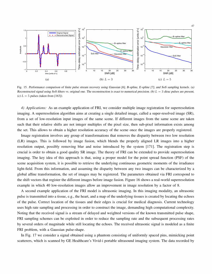
47

0 0.2 0.4 0.6 0.8 11

0.5

0

0.5

1

1.5

time [units of ]

Ampl

itude

Original SignalReconstructed Signal

(a)

5 10 15 20 25 30 35

10 6

10 4

10 2

100

102

B spline filter

Gaussian filterE spline filter

SoS filter

SNR [dB]

Tim

ede

lay

estim

atio

n er

ror [

units

of

](b) L = 3

5 10 15 20 25 30 35

10 6

10 4

10 2

100

102

B spline filter

Gaussian filter

E spline filter

SoS filter

SNR [dB]

Tim

ede

lay

estim

atio

n er

ror [

units

of

]

(c) L = 5

Fig. 15. Performance comparison of finite pulse stream recovery using Gaussian [6], B-spline, E-spline [7], and SoS sampling kernels. (a)Reconstructed signal using SoS filters vs. original one. The reconstruction is exact to numerical precision. (b) L = 3 dirac pulses are present,(c) L = 5 pulses (taken from [163]).

4) Applications: As an example application of FRI, we consider multiple image registration for superresolutionimaging. A superresolution algorithm aims at creating a single detailed image, called a super-resolved image (SR),from a set of low-resolution input images of the same scene. If different images from the same scene are takensuch that their relative shifts are not integer multiples of the pixel size, then sub-pixel information exists amongthe set. This allows to obtain a higher resolution accuracy of the scene once the images are properly registered.

Image registration involves any group of transformations that removes the disparity between two low resolution(LR) images. This is followed by image fusion, which blends the properly aligned LR images into a higherresolution output, possibly removing blur and noise introduced by the system [171]. The registration step iscrucial is order to obtain a good quality SR image. The theory of FRI can be extended to provide superresolutionimaging. The key idea of this approach is that, using a proper model for the point spread function (PSF) of thescene acquisition system, it is possible to retrieve the underlying continuous geometric moments of the irradiancelight-field. From this information, and assuming the disparity between any two images can be characterized by aglobal affine transformation, the set of images may be registered. The parameters obtained via FRI correspond tothe shift vectors that register the different images before image fusion. Figure 16 shows a real-world superresolutionexample in which 40 low-resolution images allow an improvement in image resolution by a factor of 8.

A second example application of the FRI model is ultrasonic imaging. In this imaging modality, an ultrasonicpulse is transmitted into a tissue, e.g., the heart, and a map of the underlying tissues is created by locating the echoesof the pulse. Correct location of the tissues and their edges is crucial for medical diagnosis. Current technologyuses high rate sampling and processing in order to construct the image, demanding high computational complexity.Noting that the received signal is a stream of delayed and weighted versions of the known transmitted pulse shape,FRI sampling schemes can be exploited in order to reduce the sampling rate and the subsequent processing ratesby several orders of magnitude while still locating the echoes. The received ultrasonic signal is modeled as a finiteFRI problem, with a Gaussian pulse-shape.

In Fig. 17 we consider a signal obtained using a phantom consisting of uniformly spaced pins, mimicking pointscatterers, which is scanned by GE Healthcare’s Vivid-i portable ultrasound imaging system. The data recorded by

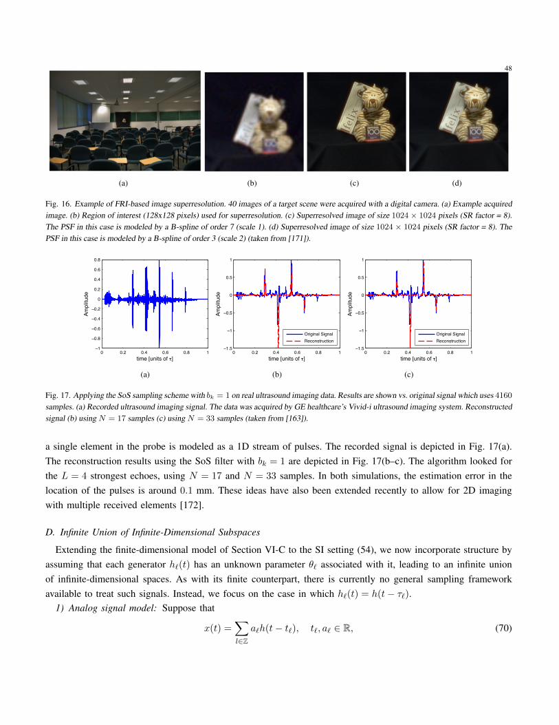
48

(a) (b) (c) (d)

Fig. 16. Example of FRI-based image superresolution. 40 images of a target scene were acquired with a digital camera. (a) Example acquiredimage. (b) Region of interest (128x128 pixels) used for superresolution. (c) Superresolved image of size 1024 × 1024 pixels (SR factor = 8).The PSF in this case is modeled by a B-spline of order 7 (scale 1). (d) Superresolved image of size 1024 × 1024 pixels (SR factor = 8). ThePSF in this case is modeled by a B-spline of order 3 (scale 2) (taken from [171]).

0 0.2 0.4 0.6 0.8 11

0.8

0.6

0.4

0.2

0

0.2

0.4

0.6

0.8

time [units of ]

Ampl

itude

(a)

0 0.2 0.4 0.6 0.8 11.5

1

0.5

0

0.5

1

time [units of ]

Ampl

itude

Original SignalReconstruction

(b)

0 0.2 0.4 0.6 0.8 11.5

1

0.5

0

0.5

1

time [units of ]Am

plitu

de

Original SignalReconstruction

(c)

Fig. 17. Applying the SoS sampling scheme with bk = 1 on real ultrasound imaging data. Results are shown vs. original signal which uses 4160

samples. (a) Recorded ultrasound imaging signal. The data was acquired by GE healthcare’s Vivid-i ultrasound imaging system. Reconstructedsignal (b) using N = 17 samples (c) using N = 33 samples (taken from [163]).

a single element in the probe is modeled as a 1D stream of pulses. The recorded signal is depicted in Fig. 17(a).The reconstruction results using the SoS filter with bk = 1 are depicted in Fig. 17(b–c). The algorithm looked forthe L = 4 strongest echoes, using N = 17 and N = 33 samples. In both simulations, the estimation error in thelocation of the pulses is around 0.1 mm. These ideas have also been extended recently to allow for 2D imagingwith multiple received elements [172].

D. Infinite Union of Infinite-Dimensional Subspaces

Extending the finite-dimensional model of Section VI-C to the SI setting (54), we now incorporate structure byassuming that each generator h`(t) has an unknown parameter θ` associated with it, leading to an infinite unionof infinite-dimensional spaces. As with its finite counterpart, there is currently no general sampling frameworkavailable to treat such signals. Instead, we focus on the case in which h`(t) = h(t− τ`).

1) Analog signal model: Suppose that

x(t) =∑

l∈Za`h(t− t`), t`, a` ∈ R, (70)

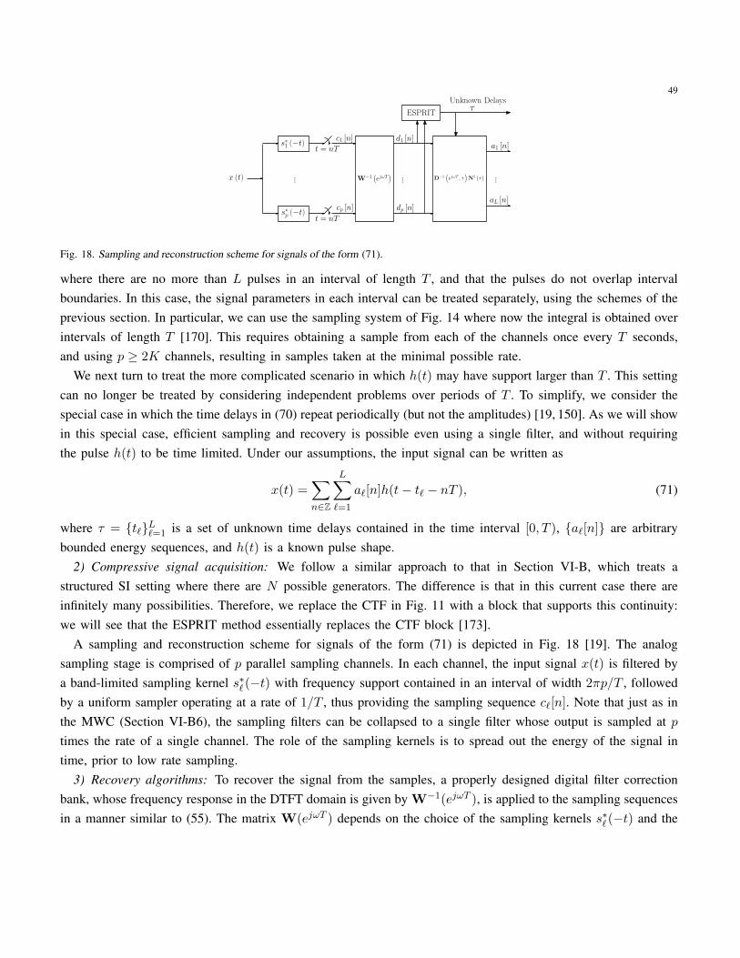
49

s!1 ("t)

...x (t)

t = nT

t = nT

...

c1 [n]

s!p ("t)

cp [n]

W"1!ej!T

"

d1 [n]

dp [n]

D!1!ej!T , !

"N† (!) ...

a1 [n]

aL [n]

ESPRIT!

Unknown Delays

Fig. 18. Sampling and reconstruction scheme for signals of the form (71).

where there are no more than L pulses in an interval of length T , and that the pulses do not overlap intervalboundaries. In this case, the signal parameters in each interval can be treated separately, using the schemes of theprevious section. In particular, we can use the sampling system of Fig. 14 where now the integral is obtained overintervals of length T [170]. This requires obtaining a sample from each of the channels once every T seconds,and using p ≥ 2K channels, resulting in samples taken at the minimal possible rate.

We next turn to treat the more complicated scenario in which h(t) may have support larger than T . This settingcan no longer be treated by considering independent problems over periods of T . To simplify, we consider thespecial case in which the time delays in (70) repeat periodically (but not the amplitudes) [19, 150]. As we will showin this special case, efficient sampling and recovery is possible even using a single filter, and without requiringthe pulse h(t) to be time limited. Under our assumptions, the input signal can be written as

x(t) =∑

n∈Z

L∑

`=1

a`[n]h(t− t` − nT ), (71)

where τ = t`L`=1 is a set of unknown time delays contained in the time interval [0, T ), a`[n] are arbitrarybounded energy sequences, and h(t) is a known pulse shape.

2) Compressive signal acquisition: We follow a similar approach to that in Section VI-B, which treats astructured SI setting where there are N possible generators. The difference is that in this current case there areinfinitely many possibilities. Therefore, we replace the CTF in Fig. 11 with a block that supports this continuity:we will see that the ESPRIT method essentially replaces the CTF block [173].

A sampling and reconstruction scheme for signals of the form (71) is depicted in Fig. 18 [19]. The analogsampling stage is comprised of p parallel sampling channels. In each channel, the input signal x(t) is filtered bya band-limited sampling kernel s∗` (−t) with frequency support contained in an interval of width 2πp/T , followedby a uniform sampler operating at a rate of 1/T , thus providing the sampling sequence c`[n]. Note that just as inthe MWC (Section VI-B6), the sampling filters can be collapsed to a single filter whose output is sampled at ptimes the rate of a single channel. The role of the sampling kernels is to spread out the energy of the signal intime, prior to low rate sampling.

3) Recovery algorithms: To recover the signal from the samples, a properly designed digital filter correctionbank, whose frequency response in the DTFT domain is given by W−1(ejωT ), is applied to the sampling sequencesin a manner similar to (55). The matrix W(ejωT ) depends on the choice of the sampling kernels s∗` (−t) and the

50Algorithm 4 ESPRIT Algorithm

Input: Signal d, number of parameters L.Output: Delays τ = t1, . . . , tL.Rdd =

∑n∈Z d [n] dH [n] construct correlation matrix

(E, σ)← SVD(Rdd) calculate SVDEs ← L singular vectors of Rdd associated with non-zero singular values.Φ = E†s↓Es↑ compute ESPRIT matrixλ1, . . . , λL ← eig(Φ) obtain eigenvaluesti ← − T

2π arg (λi), 1 ≤ i ≤ L map eigenvalues to delaysreturn τ = t1, . . . , tL

pulse shape h(t). Its entries are defined for 1 ≤ `,m ≤ p as

W(ejωT

)`,m

=1

TS∗` (ω + 2πm/T )H(ω + 2πm/T ). (72)

After the digital correction stage, it can be shown that the corrected sample vector d[n] is related to the unknownamplitude vector a[n] by a Vandermonde matrix which depends on the unknown delays [19]. Therefore, we cannow exploit known tools taken from the direction of arrival [174] and spectral estimation [164] literature to recoverthe delays τ = t1, . . . , tL, such as the well-known ESPRIT algorithm [173]. Once the delays are determined,additional filtering operations are applied on the samples to recover the sequences a`[n]. In particular, referring toFig. 18, the matrix D is a diagonal matrix with diagonal elements equal to e−jωtk , and N(τ) is a Vandermondematrix with elements e−j2πmtk/T . The ESPRIT algorithm is summarized for our setting as Algorithm 4, whereEs↓ and Es↑ denote the sub matrices extracted from Es by deleting its last/first row, respectively.

4) Recovery guarantees: The proposed algorithm is guaranteed to recover the unknown delays and amplitudesas long as p is large enough [19].

Theorem 29. [19] The sampling scheme of Fig. 18 is guaranteed to recover any signal of the form (71) as longas p ≥ 2L− η+ 1, where η is the dimension of the minimal subspace containing the vector set d[n], n ∈ Z. Inaddition, the filters s`(t) are supported on 2πp/T and must be chosen such that W(ejωT ) of (72) is invertible.

The sampling rate resulting from Theorem 29 is no larger than 2L/T since 0 ≤ η ≤ L. For certain signals, therate can be reduced to (L+1)/T . This is due to the fact that the outputs are processed jointly, similar to the MMVmodel. Evidently, the minimal sampling rate is not related to the Nyquist rate of the pulse h(t). Therefore, forwideband pulse shapes, the reduction in rate can be quite substantial. As an example, consider the setup in [175],used for characterization of ultra-wide band wireless indoor channels. Under this setup, pulses with bandwidth ofW = 1GHz are transmitted at a rate of 1/T = 2MHz. Assuming that there are 10 significant multipath components,we can reduce the sampling rate down to 40MHz compared with the 2GHz Nyquist rate.

5) Applications: Problems of the form (71) appear in a variety of different settings. For example, the model(71) can describe multipath medium identification problems, which arise in applications such as radar [176],underwater acoustics [177], wireless communications, and more. In this context, pulses with known shape are

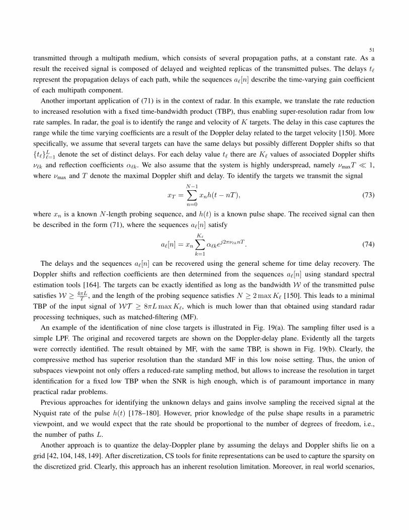
51

transmitted through a multipath medium, which consists of several propagation paths, at a constant rate. As aresult the received signal is composed of delayed and weighted replicas of the transmitted pulses. The delays t`represent the propagation delays of each path, while the sequences a`[n] describe the time-varying gain coefficientof each multipath component.

Another important application of (71) is in the context of radar. In this example, we translate the rate reductionto increased resolution with a fixed time-bandwidth product (TBP), thus enabling super-resolution radar from lowrate samples. In radar, the goal is to identify the range and velocity of K targets. The delay in this case captures therange while the time varying coefficients are a result of the Doppler delay related to the target velocity [150]. Morespecifically, we assume that several targets can have the same delays but possibly different Doppler shifts so thatt`L`=1 denote the set of distinct delays. For each delay value t` there are K` values of associated Doppler shiftsν`k and reflection coefficients α`k. We also assume that the system is highly underspread, namely νmaxT 1,where νmax and T denote the maximal Doppler shift and delay. To identify the targets we transmit the signal

xT =

N−1∑

n=0

xnh(t− nT ), (73)

where xn is a known N -length probing sequence, and h(t) is a known pulse shape. The received signal can thenbe described in the form (71), where the sequences a`[n] satisfy

a`[n] = xn

K∑

k=1

α`kej2πν`knT . (74)

The delays and the sequences a`[n] can be recovered using the general scheme for time delay recovery. TheDoppler shifts and reflection coefficients are then determined from the sequences a`[n] using standard spectralestimation tools [164]. The targets can be exactly identified as long as the bandwidth W of the transmitted pulsesatisfies W ≥ 4πL

T , and the length of the probing sequence satisfies N ≥ 2 maxK` [150]. This leads to a minimalTBP of the input signal of WT ≥ 8πLmaxK`, which is much lower than that obtained using standard radarprocessing techniques, such as matched-filtering (MF).

An example of the identification of nine close targets is illustrated in Fig. 19(a). The sampling filter used is asimple LPF. The original and recovered targets are shown on the Doppler-delay plane. Evidently all the targetswere correctly identified. The result obtained by MF, with the same TBP, is shown in Fig. 19(b). Clearly, thecompressive method has superior resolution than the standard MF in this low noise setting. Thus, the union ofsubspaces viewpoint not only offers a reduced-rate sampling method, but allows to increase the resolution in targetidentification for a fixed low TBP when the SNR is high enough, which is of paramount importance in manypractical radar problems.

Previous approaches for identifying the unknown delays and gains involve sampling the received signal at theNyquist rate of the pulse h(t) [178–180]. However, prior knowledge of the pulse shape results in a parametricviewpoint, and we would expect that the rate should be proportional to the number of degrees of freedom, i.e.,the number of paths L.

Another approach is to quantize the delay-Doppler plane by assuming the delays and Doppler shifts lie on agrid [42, 104, 148, 149]. After discretization, CS tools for finite representations can be used to capture the sparsity onthe discretized grid. Clearly, this approach has an inherent resolution limitation. Moreover, in real world scenarios,

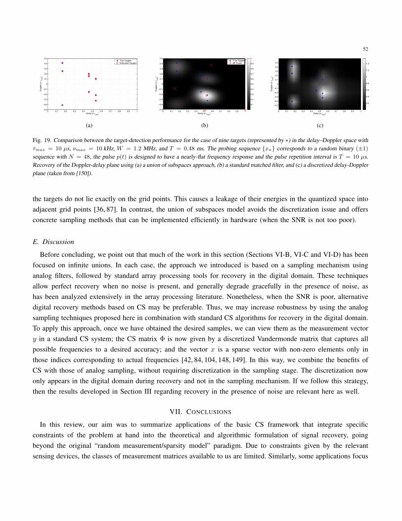
52

0 0.1 0.2 0.3 0.4 0.5 0.6 0.7 0.8 0.9 10.5

0.4

0.3

0.2

0.1

0

0.1

0.2

0.3

0.4

0.5

Delay (x max)

Dop

pler

(x

max

)

True TargetsEstimated Targets

(a)

0 0.1 0.2 0.3 0.4 0.5 0.6 0.7 0.8 0.9 10.5

0.4

0.3

0.2

0.1

0

0.1

0.2

0.3

0.4

0.5

Delay (x max)

Dop

pler

(x

max

)

0.1

0.2

0.3

0.4

0.5

0.6

0.7

0.8

0.9

1True TargetsMF Peaks

(b)

Delay (x max)

Dop

pler

(x

max

)

0 0.1 0.2 0.3 0.4 0.5 0.6 0.7 0.8 0.9 1

0.5

0.4

0.3

0.2

0.1

0

0.1

0.2

0.3

0.4

0.5

0.2

0.4

0.6

0.8

1

1.2

1.4

(c)

Fig. 19. Comparison between the target-detection performance for the case of nine targets (represented by ∗) in the delay–Doppler space withτmax = 10 µs, νmax = 10 kHz, W = 1.2 MHz, and T = 0.48 ms. The probing sequence xn corresponds to a random binary (±1)

sequence with N = 48, the pulse p(t) is designed to have a nearly-flat frequency response and the pulse repetition interval is T = 10 µs.Recovery of the Doppler-delay plane using (a) a union of subspaces approach, (b) a standard matched filter, and (c) a discretized delay-Dopplerplane (taken from [150]).

the targets do not lie exactly on the grid points. This causes a leakage of their energies in the quantized space intoadjacent grid points [36, 87]. In contrast, the union of subspaces model avoids the discretization issue and offersconcrete sampling methods that can be implemented efficiently in hardware (when the SNR is not too poor).

E. Discussion

Before concluding, we point out that much of the work in this section (Sections VI-B, VI-C and VI-D) has beenfocused on infinite unions. In each case, the approach we introduced is based on a sampling mechanism usinganalog filters, followed by standard array processing tools for recovery in the digital domain. These techniquesallow perfect recovery when no noise is present, and generally degrade gracefully in the presence of noise, ashas been analyzed extensively in the array processing literature. Nonetheless, when the SNR is poor, alternativedigital recovery methods based on CS may be preferable. Thus, we may increase robustness by using the analogsampling techniques proposed here in combination with standard CS algorithms for recovery in the digital domain.To apply this approach, once we have obtained the desired samples, we can view them as the measurement vectory in a standard CS system; the CS matrix Φ is now given by a discretized Vandermonde matrix that captures allpossible frequencies to a desired accuracy; and the vector x is a sparse vector with non-zero elements only inthose indices corresponding to actual frequencies [42, 84, 104, 148, 149]. In this way, we combine the benefits ofCS with those of analog sampling, without requiring discretization in the sampling stage. The discretization nowonly appears in the digital domain during recovery and not in the sampling mechanism. If we follow this strategy,then the results developed in Section III regarding recovery in the presence of noise are relevant here as well.

VII. CONCLUSIONS

In this review, our aim was to summarize applications of the basic CS framework that integrate specificconstraints of the problem at hand into the theoretical and algorithmic formulation of signal recovery, goingbeyond the original “random measurement/sparsity model” paradigm. Due to constraints given by the relevantsensing devices, the classes of measurement matrices available to us are limited. Similarly, some applications focus

53

on signals that exhibit structure which cannot be captured by sparsity alone and provide additional informationthat can be leveraged during signal recovery. We also considered the transition between continuous and discreterepresentations bridged by analog-to-digital converters. Analog signals are continuous-time by nature; in manycases, the application of compressed sensing to this larger signal class requires the formulation of new devices,signal models, and recovery algorithms. It also necessitates a deeper understanding of hardware considerations thatmust be taken into account in theoretical developments. This acquisition framework, in turn, motivates the designof new sampling schemes and devices that provide the information required for signal recovery in the smallestpossible representation.

While it is difficult to cover all of the developments in compressive sensing theory and hardware [66–68, 181–184], our aim here was to select few examples that were representative of wider classes of problems and thatoffered a balance between a useful theoretical background and varied applications. We hope that this summarywill be useful to practitioners in signal acquisition and processing that are interested in leveraging the features ofcompressive sensing in their specific applications. We also hope that this review will inspire further developmentsin the theory and practice underlying CS: we particularly envision extending the existing framework to broadersignals sets and inspiring new implementation and design paradigms. With an eye to the future, more advancedconfigurations of CS can play a key role in many new frontiers. Some examples already mentioned throughoutare cognitive radio, optical systems, medical devices such as MRI, ultrasound and more. These techniques holdpromise for a complete rethinking of many acquisition systems and stretch the limit of current sensing capabilities.

As we have also demonstrated, CS holds promise for increasing resolution by exploiting signal structure. Thiscan revolutionize many applications such as radar and microscopy by making efficient use of the available degreesof freedom in these settings. Consumer electronics, microscopy, civilian and military surveillance, medical imaging,radar and many other rely on ADCs and are resolution-limited. Removing the Nyquist barrier in these applicationsand increasing resolution can improve the user experience, increase data transfer, improve imaging quality andreduce exposure time – in other words, make a prominent impact on the analog-digital world surrounding us.

VIII. ACKNOWLEDGEMENTS

The authors would like to thank their colleagues for many useful comments and for their collaboration on manytopics related to this review. In particular, they are grateful to Mike Wakin for many discussions on the structure ofthe review, to Moshe Mishali, Holger Rauhut, Justin Romberg, Yao Xie, and the anonymous reviewers for offeringmany helpful comments on an early draft of the manuscript, and to Pier Luigi Dragotti, Polina Golland, LaurentJacques, Yehia Massoud, Justin Romberg, and Rebecca Willett for authorizing the use of their figures.

REFERENCES

[1] D. L. Donoho, “Compressed sensing,” IEEE Trans. Info. Theory, vol. 52, no. 4, pp. 1289–1306, Sep. 2006.[2] E. J. Candes and T. Tao, “Near optimal signal recovery from random projections: Universal encoding strategies?,” IEEE Trans. Info.

Theory, vol. 52, no. 12, pp. 5406–5425, Dec. 2006.[3] R. G. Baraniuk, “Compressive sensing,” IEEE Signal Proc. Mag., vol. 24, no. 4, pp. 118–120, 124, July 2007.[4] E. J. Candes, “Compressive sampling,” in Int. Congress of Mathematicians, Madrid, Spain, 2006, vol. 3, pp. 1433–1452.[5] E. J. Candes and M. B. Wakin, “An introduction to compressive sampling,” IEEE Signal Proc. Mag., vol. 25, no. 2, pp. 21–30, Mar.

2008.

54

[6] M. Vetterli, P. Marziliano, and T. Blu, “Sampling signals with finite rate of innovation,” IEEE Trans. Signal Proc., vol. 50, no. 6,pp. 1417–1428, 2002.

[7] P. L. Dragotti, M. Vetterli, and T. Blu, “Sampling moments and reconstructing signals of finite rate of innovation: Shannon meetsStrang-Fix,” IEEE Trans. Signal Proc., vol. 55, no. 5, pp. 1741–1757, May 2007.

[8] T. Blu, P.-L. Dragotti, M. Vetterli, P. Marziliano, and L. Coulot, “Sparse sampling of signal innovations,” IEEE Signal Proc. Mag.,vol. 25, no. 2, pp. 31–40, Mar. 2008.

[9] M. Mishali, Y. C. Eldar, O. Dounaevsky, and E. Shoshan, “Xampling: Analog to digital at sub-nyquist rates,” IET Circuits, Devicesand Systems, vol. 5, no. 1, pp. 8–20, Jan. 2011.

[10] M. Mishali and Y. C. Eldar, “Xampling: Compressed sensing for analog signals,” in Compressed Sensing: Theory and Applications,Y. C. Eldar and G. Kutyniok, Eds. Cambridge Univ. Press, 2012.

[11] H. Nyquist, “Certain topics in telegraph transmission theory,” Trans. AIEE, vol. 47, pp. 617–644, Apr. 1928.[12] C. E. Shannon, “Communications in the presence of noise,” Proc. IRE, vol. 37, pp. 10–21, Jan 1949.[13] E. T. Whittaker, “On the functions which are represented by the expansions of the interpolation theory,” Proc. Roy. Soc. Edinburgh,

vol. 35, pp. 181–194, 1915.[14] V. A. Kotelnikov, “On the transmission capacity of the ‘ether’ and of cables in electrical communications,” in All-Union Conf.

Technological Reconstruction of the Communications Sector and the Development of Low-current Engineering, 1933.[15] Y. M. Lu and M. N. Do, “A theory for sampling signals from a union of subspaces,” IEEE Trans. Signal Proc., vol. 56, no. 6, pp.

2334–2345, 2008.[16] T. Blumensath and M. E. Davies, “Sampling theorems for signals from the union of finite-dimensional linear subspaces,” IEEE

Trans. Info. Theory, vol. 55, no. 4, pp. 1872–1882, Apr. 2009.[17] Y. C. Eldar and M. Mishali, “Robust recovery of signals from a structured union of subspaces,” IEEE Trans. Info. Theory, vol. 55,

no. 11, pp. 5302–5316, 2009.[18] Y. C. Eldar, “Compressed sensing of analog signals in shift-invariant spaces,” IEEE Trans. Signal Proc., vol. 57, no. 8, pp. 2986–2997,

Aug. 2009.[19] K. Gedalyahu and Y. C. Eldar, “Time delay estimation from low rate samples: A union of subspaces approach,” IEEE Trans. Signal

Proc., vol. 58, no. 6, pp. 3017–3031, June 2010.[20] R. G. Baraniuk, V. Cevher, M. F. Duarte, and C. Hegde, “Model-based compressive sensing,” IEEE Trans. Info. Theory, vol. 56,

no. 4, pp. 1982–2001, Apr. 2010.[21] I. F. Gorodnitsky and B. D. Rao, “Sparse signal reconstruction from limited data using FOCUSS: A re-weighted minimum norm

algorithm,” IEEE Trans. Signal Proc., vol. 45, no. 3, pp. 600–616, Mar. 1997.[22] S. Chen, D. L. Donoho, and M. Saunders, “Atomic decomposition by basis pursuit,” SIAM J. Sci. Computing, vol. 20, no. 1, pp.

33–61, 1998.[23] A. M. Bruckstein, D. L. Donoho, and M. Elad, “From sparse solutions of systems of equations to sparse modeling of signals and

images,” SIAM Review, vol. 51, no. 1, pp. 34–81, Feb. 2009.[24] S. Mallat and Z. Zhang, “Matching pursuit with time-frequency dictionaries,” IEEE Trans. Signal Proc., vol. 41, no. 12, pp.

3397–3415, Dec. 1993.[25] S. Foucart, “A note on guaranteed sparse recovery via `1-minimization,” Appl. Comput. Harmon. Anal., vol. 29, no. 1, pp. 97 – 103,

2010.[26] S. Foucart and R. Gribonval, “Real versus complex null space properties for sparse vector recovery,” C. R. Acad. Sci. Paris, Ser. I,

vol. 348, no. 15–16, pp. 863–865, 2010.[27] A. Cohen, W. Dahmen, and R. A. DeVore, “Compressed sensing and best k-term approximation,” J. American Math. Society, vol.

22, no. 1, pp. 211–231, Jan. 2009.[28] D. L. Donoho and M. Elad, “Optimally sparse representation in general (nonorthogonal) dictionaries via `1 minimization,” Proc.

Nat. Acad. Sci., vol. 100, no. 5, pp. 2197–2202, Mar. 2003.[29] D.L. Donoho and Xiaoming Huo, “Uncertainty principles and ideal atomic decompositions,” IEEE Trans. Info. Theory, vol. 47, no.

7, pp. 2845–2862, Nov. 2001.[30] J. A. Tropp, “Greed is good: Algorithmic results for sparse approximation,” IEEE Trans. Info. Theory, vol. 50, no. 10, pp. 2231–2242,

Oct. 2004.

55

[31] R. Gribonval and M. Nielsen, “Sparse representations in unions of bases,” IEEE Trans. Info. Theory, vol. 49, no. 12, pp. 3320–3325,Dec. 2003.

[32] L. R. Welch, “Lower bounds on the maximum cross correlation of signals,” IEEE Trans. Info. Theory, vol. 20, no. 3, pp. 397–399,May 1974.

[33] T. Strohmer and R. Heath, “Grassmanian frames with applications to coding and communication,” Appl. Comput. Harmon. Anal.,vol. 14, no. 3, pp. 257–275, Nov. 2003.

[34] S. A. Gersgorin, “Uber die abgrenzung der eigenwerte einer matrix,” Izv. Akad. Nauk SSSR Ser. Fiz.-Mat., vol. 6, pp. 749–754, 1931.[35] M.A. Herman and T. Strohmer, “General deviants: An analysis of perturbations in compressed sensing,” IEEE J. Selected Topics in

Signal Proc., vol. 4, no. 2, pp. 342 –349, Apr. 2010.[36] Y. Chi, L. L. Scharf, A. Pezeshki, and R. Calderbank, “Sensitivity to basis mismatch in compressed sensing,” IEEE Trans. Signal

Proc., vol. 59, no. 5, pp. 2182–2195, May 2011.[37] J. Treichler, M. A. Davenport, and R. G. Baraniuk, “Application of compressive sensing to the design of wideband signal acquisition

receivers,” in U.S./Australia Joint Workshop on Defense Applications of Signal Proc. (DASP), Lihue, HI, Sep. 2009.[38] S. Aeron, V. Saligrama, and M. Zhao, “Information theoretic bounds for compressed sensing,” IEEE Trans. Info. Theory, vol. 56,

no. 10, pp. 5111–5130, Oct. 2010.[39] Z. Ben-Haim, T. Michaeli, and Y. C. Eldar, “Performance bounds and design criteria for estimating finite rate of innovation signals,”

Sep. 2010, Preprint, arXiv:1009.2221.[40] E. Arias-Castro and Y. C. Eldar, “Noise folding in compressed sensing,” IEEE Signal Proc. Letters, 2011, To appear.[41] T. T. Cai, G. Xu, and J. Zhang, “On recovery of sparse signals via `1 minimization,” IEEE Trans. Info. Theory, vol. 55, no. 7, pp.

3388–3397, July 2009.[42] M. A. Herman and T. Strohmer, “High-resolution radar via compressed sensing,” IEEE Trans. Signal Proc., vol. 57, no. 6, pp.

2275–2284, June 2009.[43] R. A. DeVore, “Deterministic constructions of compressed sensing matrices,” J. Complex., vol. 23, no. 4, pp. 918–925, Aug. 2007.[44] D. Donoho, “For most large underdetermined systems of linear equations, the minimal `1-norm solution is also the sparsest solution,”

Comm. Pure Appl. Math., vol. 59, no. 6, pp. 797–829, 2006.[45] E. J. Candes and Y. Plan, “Near-ideal model selection by `1 minimization,” Ann. Stat., vol. 37, no. 5A, pp. 2145–2177, Oct. 2009.[46] R. G. Baraniuk, M. Davenport, R. DeVore, and M. Wakin, “A simple proof of the restricted isometry property for random matrices,”

Constructive Approximation, vol. 28, no. 3, pp. 253–263, 2008.[47] D. L. Donoho and J. Tanner, “Observed universality of phase transitions in high-dimensional geometry, with implications for modern

data analysis and signal processing,” Phil. Trans. Royal Soc. A, vol. 367, no. 1906, pp. 4273–4293, Nov. 2009.[48] C. Dossal, G. Peyre, and J. Fadili, “A numerical exploration of compressed sampling recovery,” Linear Algebra and its Applications,

vol. 432, no. 7, pp. 1663 – 1679, Mar. 2010.[49] S. Boyd and L. Vanderberghe, Convex Optimization, Cambridge Univ. Press, 2004.[50] L. I. Rudin, S. Osher, and E. Fatemi, “Nonlinear total variation based noise removal algorithms,” Phys. D, vol. 60, pp. 259–268,

Nov. 1992.[51] J.A. Tropp and S.J. Wright, “Computational methods for sparse solution of linear inverse problems,” Proc. IEEE, vol. 98, no. 6, pp.

948 –958, June 2010.[52] J. Haupt and R. Nowak, “Signal reconstruction from noisy random projections,” IEEE Trans. Info. Theory, vol. 52, no. 9, pp.

4036–4048, Sep. 2006.[53] S. Ji, Y. Xue, and L. Carin, “Bayesian compressive sensing,” IEEE Trans. Signal Proc., vol. 56, no. 6, pp. 2346–2356, June 2008.[54] E. Candes and T. Tao, “The Dantzig selector: Statistical estimation when p is much larger than n,” Ann. Stat., vol. 35, no. 6, pp.

2313–2351, Dec. 2005.[55] Y. Pati, R. Rezaifar, and P. Krishnaprasad, “Orthogonal matching pursuit: Recursive function approximation with applications to

wavelet decomposition,” in Asilomar Conf. Signals, Systems, and Computers, Pacific Grove, CA, Nov. 1993.[56] D. Needell and J. A. Tropp, “CoSaMP: Iterative signal recovery from incomplete and inaccurate samples,” Appl. Comput. Harmon.

Anal., vol. 26, no. 3, pp. 301–321, May 2008.[57] W. Dai and O. Milenkovic, “Subspace pursuit for compressive sensing signal reconstruction,” IEEE Trans. Info. Theory, vol. 55,

no. 5, pp. 2230–2249, May 2009.

56

[58] T. Blumensath and M. E. Davies, “Iterative hard thresholding for compressed sensing,” Appl. Comput. Harmon. Anal., vol. 27, no.3, pp. 265–274, Nov. 2008.

[59] D. L. Donoho, M. Elad, and V. N. Temlyakov, “Stable recovery of sparse overcomplete representations in the presence of noise,”IEEE Trans. Info. Theory, vol. 52, no. 1, pp. 6–18, Jan. 2006.

[60] E. J. Candes, J. K. Romberg, and T. Tao, “Stable signal recovery from incomplete and inaccurate measurements,” Comm. Pure Appl.Math., vol. 59, no. 8, pp. 1207–1223, 2006.

[61] Z. Ben-Haim, Y. C. Eldar, and M. Elad, “Coherence-based performance guarantees for estimating a sparse vector under randomnoise,” IEEE Trans. Signal Proc., vol. 58, no. 10, pp. 5030–5043, Oct. 2010.

[62] Z. Ben-Haim and Y. C. Eldar, “The Cramer-Rao bound for estimating a sparse parameter vector,” IEEE Trans. Signal Proc., vol.58, no. 6, pp. 3384–3389, June 2010.

[63] M. B. Wakin and M. A. Davenport, “Analysis of orthogonal matching pursuit using the restricted isometry property,” IEEE Trans.Info. Theory, vol. 56, no. 9, pp. 4395–4401, Sep. 2010.

[64] T. Zhang, “Sparse recovery with orthogonal matching pursuit under RIP,” May 2010, Preprint, arXiv:1005.2449.[65] J. A. Tropp, “On the conditioning of random subdictionaries,” Appl. Comput. Harmon. Anal., vol. 25, pp. 1–24, 2008.[66] M. E. Gehm, R. John, D. Brady, R. Willett, and T. J. Schulz, “Single-shot compressive spectral imaging with a dual-disperser

architecture,” Optics Express, vol. 15, no. 21, pp. 14013–14027, Oct. 2007.[67] M. A. Neifeld and J. Ke, “Optical architectures for compressive imaging,” Appl. Optics, vol. 46, no. 22, pp. 5293–5303, July 2007.[68] A. Wagadarikar, R. John, R. Willett, and D. Brady, “Single disperser design for coded aperture snapshot spectral imaging,” Appl.

Optics, vol. 47, no. 10, pp. B44–B51, Apr. 2008.[69] E. J. Candes and J. K. Romberg, “Sparsity and incoherence in compressive sampling,” Inverse Problems, vol. 23, no. 3, pp. 969–985,

2007.[70] Y. C. Eldar, “Uncertainty relations for shift-invariant analog signals,” IEEE Trans. Info. Theory, vol. 55, no. 12, pp. 5742–5757,

Dec. 2009.[71] M. Rudelson and R. Vershynin, “On sparse reconstruction from Fourier and Gaussian measurements,” Comm. Pure Appl. Math.,

vol. 61, no. 8, pp. 1025–1171, Aug. 2008.[72] M. Lustig, D. L. Donoho, J. M. Santos, and J. M. Pauly, “Compressed sensing MRI,” IEEE Signal Proc. Mag., vol. 25, no. 2, pp.

72–82, Mar. 2008.[73] E. J. Candes, J. K. Romberg, and T. Tao, “Robust uncertainty principles: Exact signal reconstruction from highly incomplete frequency

information,” IEEE Trans. Info. Theory, vol. 52, no. 2, pp. 489–509, 2006.[74] S. Gazit, A. Szameit, Y. C. Eldar, and M. Segev, “Super-resolution and reconstruction of sparse sub-wavelength images,” Opt.

Express, vol. 17, pp. 23920–23946, 2009.[75] Y. Shechtman, S. Gazit, A. Szameit, Y. C. Eldar, and M. Segev, “Super-resolution and reconstruction of sparse images carried by

incoherent light,” Opt. Letters, vol. 35, pp. 23920–23946, April 2010.[76] M. F. Duarte, M. A. Davenport, D. Takhar, J. N. Laska, T. Sun, K. F. Kelly, and R. G. Baraniuk, “Single pixel imaging via compressive

sampling,” IEEE Signal Proc. Mag., vol. 25, no. 2, pp. 83–91, March 2008.[77] R. Coifman, F. Geshwind, and Y. Meyer, “Noiselets,” Appl. Comp. Harmonic Analysis, vol. 10, pp. 27–44, 2001.[78] R. A. DeVerse, R. R. Coifman, A. C. Coppi, W. G. Fateley, F. Geshwind, R. M. Hammaker, S. Valenti, F. J. Warner, and G. L. Davis,

“Application of spatial light modulators for new modalities in spectrometry and imaging,” in Spectral Imaging: Instrumentation,Applications, and Analysis II, San Jose, CA, Jan. 2003, vol. 4959 of Proc. SPIE, pp. 12–22.

[79] W. L. Chan, K. Charan, D. Takhar, K. F. Kelly, R. G. Baraniuk, and D. M. Mittleman, “A single-pixel terahertz imaging systembased on compressed sensing,” Appl. Phy. Letters, vol. 93, no. 12, Sep. 2008.

[80] P. Ye, J. L. Paredes, G. R. Arce, Y. Wu, C. Chen, and D. W. Prather, “Compressive confocal microscopy,” in IEEE Int. Conf.Acoustics, Speech, and Signal Proc. (ICASSP), Taipei, Taiwan, Apr. 2009, pp. 429–432.

[81] S. Pfetsch, T. Ragheb, J. Laska, H. Nejati, A. Gilbert, M. Strauss, R. Baraniuk, and Y. Massoud, “On the feasibility of hardwareimplementation of sub-nyquist random-sampling based analog-to-information conversion,” in IEEE Int. Symp. Circuits and Systems(ISCAS), Seattle, WA, May 2008, pp. 1480–1483.

[82] A.C. Gilbert, M.J. Strauss, and J.A. Tropp, “A tutorial on fast fourier sampling,” IEEE Signal Proc. Mag., vol. 25, no. 2, pp. 57–66,Mar. 2008.

57

[83] W. U. Bajwa, A. Sayeed, and R. Nowak, “A restricted isometry property for structurally subsampled unitary matrices,” in AllertonConf. Communication, Control, and Computing, Monticello, IL, Sep. 2009, pp. 1005–1012.

[84] J. A. Tropp, J. N. Laska, M. F. Duarte, J. K. Romberg, and R. G. Baraniuk, “Beyond Nyquist: Efficient sampling of sparse bandlimitedsignals,” IEEE Trans. Info. Theory, vol. 56, no. 1, pp. 520–544, Jan. 2010.

[85] T. Ragheb, J. N. Laska, H. Nejati, S. Kirolos, R. G. Baraniuk, and Y. Massoud, “A prototype hardware for random demodulationbased compressive analog-to-digital conversion,” in IEEE Midwest Symp. Circuits and Systems, Knoxville, TN, Aug. 2008, pp. 37–40.

[86] Z. Yu, S. Hoyos, and B. M. Sadler, “Mixed-signal parallel compressed sensing and reception for cognitive radio,” in IEEE Int. Conf.Acoustics, Speech, and Signal Proc. (ICASSP), Las Vegas, NV, Apr. 2008, pp. 3861–3864.

[87] M. F. Duarte and R. G. Baraniuk, “Spectral compressive sensing,” Feb. 2010, Preprint.[88] G. C. Valley and T. J. Shaw, “Compressive sensing recovery of sparse signals with arbitrary frequencies,” 2010, Preprint.[89] J. D. Haupt, W. U. Bajwa, G. Raz, and R. Nowak, “Toeplitz compressed sensing matrices with applications to sparse channel

estimation,” IEEE Trans. Info. Theory, vol. 56, no. 11, pp. 5862–5875, June 2010.[90] H. Rauhut, “Compressive sensing and structured random matrices,” in Theoretical Foundations and Numerical Methods for Sparse

Recovery, H. Rauhut, Ed., vol. 9 of Radon Series on Computational and Applied Mathematics. De Gruyter, 2010.[91] H. Rauhut, J. K. Romberg, and J. A. Tropp, “Restricted isometries for partial random circulant matrices,” Appl. Comput. Harmon.

Anal., May 2011, To appear.[92] J. K. Romberg, “Compressive sensing by random convolution,” SIAM J. Imaging Science, vol. 2, no. 4, pp. 1098–1128, Dec. 2009.[93] R. F. Marcia and R. M. Willett, “Compressive coded aperture superresolution image reconstruction,” in IEEE Int. Conf. Acoustics,

Speech, and Signal Proc. (ICASSP), Las Vegas, NV, USA, March 2008, pp. 833–836.[94] R. Marcia, Z. Harmany, and R. Willett, “Compressive coded aperture imaging,” in Computational Imaging VII, San Jose, CA, Jan.

2009, vol. 7246 of Proc. SPIE.[95] L. Jacques, P. Vandergheynst, A. Bibet, V. Majidzadeh, A. Schmid, and Y. Leblebici, “CMOS compressed imaging by random

convolution,” in IEEE Int. Conf. Acoustics, Speech, and Signal Proc. (ICASSP), Taipei, Taiwan, Apr. 2009, pp. 1113–1116.[96] M. F. Duarte and R. G. Baraniuk, “Kronecker compressive sensing,” 2009, Preprint.[97] Y. Rivenson and A. Stern, “Compressed imaging with a separable sensing operator,” IEEE Signal Proc. Letters, vol. 16, no. 6, pp.

449–452, June 2009.[98] T. Sun and K. F. Kelly, “Compressive sensing hyperspectral imager,” in Computational Optical Sensing and Imaging (COSI), San

Jose, CA, Oct. 2009.[99] R. Robucci, J. Gray, L. K. Chiu, J. K. Romberg, and P. Hasler, “Compressive sensing on a CMOS separable-transform image sensor,”

Proc. IEEE, vol. 98, no. 6, pp. 1089–1101, June 2010.[100] R. A. Horn and C. R. Johnson, Topics in matrix analysis, Cambridge University Press, 1991.[101] D. Baron, M. B. Wakin, M. F. Duarte, S. Sarvotham, and R. G. Baraniuk, “Distributed compressed sensing,” Tech. Rep. TREE-0612,

Rice University, Department of Electrical and Computer Engineering, Houston, TX, Nov. 2006.[102] J. W. Phillips, R. M. Leahy, and J. C. Mosher, “MEG-based imaging of focal neuronal current sources,” IEEE Trans. Medical

Imaging, vol. 16, no. 3, pp. 338–348, June 1997.[103] R. Gribonval, “Sparse decomposition of stereo signals with matching pursuit and application to blind separation of more than two

sources from a stereo mixture,” in IEEE Int. Conf. Acoustics, Speech, and Signal Proc. (ICASSP), Minneapolis, MN, Apr. 1993.[104] D. Malioutov, M. Cetin, and A. S. Willsky, “A sparse signal reconstruction perspective for source localization with sensor arrays,”

IEEE Trans. Signal Proc., vol. 53, no. 8, pp. 3010–3022, Aug. 2005.[105] S. F. Cotter and B. D. Rao, “Sparse channel estimation via matching pursuit with application to equalization,” IEEE Trans.

Communications, vol. 50, no. 3, pp. 374–377, Mar. 2002.[106] I. J. Fevrier, S. B. Gelfand, and M. P. Fitz, “Reduced complexity decision feedback equalization for multipath channels with large

delay spreads,” IEEE Trans. Communications, vol. 47, no. 6, pp. 927–937, June 1999.[107] J. A. Bazerque and G. B. Giannakis, “Distributed spectrum sensing for cognitive radio networks by exploiting sparsity,” IEEE Trans.

Signal Proc., vol. 58, no. 3, pp. 1847–1862, Mar. 2010.[108] M. Mishali and Y. C. Eldar, “Blind multiband signal reconstruction: Compressed sensing for analog signals,” IEEE Trans. Signal

Proc., vol. 57, pp. 993–1009, Mar. 2009.[109] M. Mishali and Y. C. Eldar, “From theory to practice: Sub-Nyquist sampling of sparse wideband analog signals,” IEEE J. Selected

Topics in Signal Proc., vol. 4, no. 2, pp. 375–391, Apr. 2010.

58

[110] M. E. Davies and Y. C. Eldar, “Rank awareness in joint sparse recovery,” Apr. 2010, Preprint, arXiv:1004.4529.[111] P. Feng, Universal minimum-rate sampling and spectrum-blind reconstruction for multiband signals, Ph.D. thesis, University of

Illinois, Urbana, IL, 1998.[112] J. Chen and X. Huo, “Theoretical results on sparse representations of multiple-measurement vectors,” IEEE Trans. Signal Proc.,

vol. 54, no. 12, pp. 4634–4643, Dec. 2006.[113] M. Mishali and Y. C. Eldar, “Reduce and boost: Recovering arbitrary sets of jointly sparse vectors,” IEEE Trans. Signal Proc., vol.

56, no. 10, pp. 4692–4702, Oct. 2008.[114] J. A. Tropp, A. C. Gilbert, and M. J. Strauss, “Algorithms for simultaneous sparse approximation. Part I: Greedy pursuit,” Signal

Proc., vol. 86, pp. 572–588, Apr. 2006.[115] J. A. Tropp, “Algorithms for simultaneous sparse approximation. Part II: Convex relaxation,” Signal Proc., vol. 86, pp. 589–602,

Apr. 2006.[116] M. Fornasier and H. Rauhut, “Recovery algorithms for vector valued data with joint sparsity constraints,” SIAM J. Numer. Anal.,

vol. 46, no. 2, pp. 577–613, 2008.[117] S. F. Cotter, B. D. Rao, K. Engan, and K. Kreutz-Delgado, “Sparse solutions to linear inverse problems with multiple measurement

vectors,” IEEE Trans. Signal Proc., vol. 53, no. 7, pp. 2477–2488, July 2005.[118] R. Gribonval, H. Rauhut, K. Schnass, and P. Vandergheynst, “Atoms of all channels, unite! Average case analysis of multi-channel

sparse recovery using greedy algorithms,” J. Fourier Anal. Appl., vol. 14, no. 5, pp. 655–687, 2008.[119] Y. C. Eldar and H. Rauhut, “Average case analysis of multichannel sparse recovery using convex relaxation,” IEEE Trans. Info.

Theory, vol. 6, no. 1, pp. 505–519, Jan. 2010.[120] Y. C. Eldar, P. Kuppinger, and H. Bolcskei, “Block-sparse signals: Uncertainty relations and efficient recovery,” IEEE Trans. Signal

Proc., pp. 3042–3054, June 2010.[121] R. O. Schmidt, “Multiple emitter location and signal parameter estimation,” in RADC Spectral Estimation Workshop, Rome, NY,

Oct. 1979, pp. 243–258.[122] P. Feng and Y. Bresler, “Spectrum-blind minimum-rate sampling and reconstruction of multiband signals,” in IEEE Int. Conf.

Acoustics, Speech, and Signal Proc. (ICASSP), Atlanta, GA, May. 1996, vol. 3, pp. 1688–1691.[123] K. Schnass and P. Vandergheynst, “Average performance analysis for thresholding,” IEEE Signal Proc. Letters, vol. 14, no. 11, pp.

828–831, Nov. 2007.[124] W. Ou, M. S. Hamalainen, and P. Golland, “A distributed spatio-temporal EEG/MEG inverse solver,” Neuroimage, vol. 44, no. 3,

pp. 932–946, Feb. 2009.[125] V. Cevher, M. F. Duarte, C. Hegde, and R. G. Baraniuk, “Sparse signal recovery using Markov Random Fields,” in Workshop on

Neural Info. Proc. Systems (NIPS), Vancouver, Canada, Dec. 2008.[126] P. Schniter, “Turbo reconstruction of structured sparse signals,” in Conf. Info. Sci. and Sys. (CISS), Princeton, NJ, Mar. 2010.[127] D. Baron, S. Sarvotham, and R.G. Baraniuk, “Bayesian compressive sensing via belief propagation,” IEEE Trans. Signal Proc., vol.

58, no. 1, pp. 269 –280, Jan. 2010.[128] L. He and L. Carin, “Exploiting structure in wavelet-based Bayesian compressive sensing,” IEEE Trans. Signal Proc., vol. 57, no.

9, pp. 3488–3497, Sep. 2009.[129] S. Ji, D. Dunson, and L. Carin, “Multi-task compressive sensing,” IEEE Trans. Signal Proc., vol. 57, no. 1, pp. 92–106, Jan. 2009.[130] L. He, H. Chen, and L. Carin, “Tree-structured compressive sensing with variational Bayesian analysis,” IEEE Signal Proc. Letters,

vol. 17, no. 3, pp. 233–236, Mar. 2010.[131] T. Faktor, Y. C. Eldar, and M. Elad, “Exploiting statistical dependencies in sparse representations for signal recovery,” Oct. 2010,

Preprint, arXiv:1010.5734.[132] R. Jenatton, J. Y. Audibert, and F. Bach, “Structured variable selection with sparsity inducing norms,” April 2009, Preprint,

arXiv:0904.3523.[133] L. Peotta and P. Vandergheynst, “Matching pursuit with block incoherent dictionaries,” IEEE Trans. Signal Proc., vol. 55, no. 9, pp.

4549–4557, Sep. 2007.[134] M. Yuan and Y. Lin, “Model selection and estimation in regression with grouped variables,” J. Roy. Stat. Soc. Ser. B Stat. Methodol.,

vol. 68, no. 1, pp. 49–67, 2006.[135] Y. C. Eldar and T. Michaeli, “Beyond bandlimited sampling,” IEEE Signal Proc. Mag., vol. 26, no. 3, pp. 48–68, May 2009.[136] F. R. Bach, “Consistency of the group lasso and multiple kernel learning,” J. Mach. Learn. Res., vol. 9, pp. 1179–1225, 2008.

59

[137] Y. Nardi and A. Rinaldo, “On the asymptotic properties of the group lasso estimator for linear models,” Electron. J. Statist., vol. 2,pp. 605–633, 2008.

[138] M. Stojnic, F. Parvaresh, and B. Hassibi, “On the reconstruction of block-sparse signals with an optimal number of measurements,”IEEE Trans. Signal Proc., vol. 57, no. 8, pp. 3075–3085, Aug. 2009.

[139] L. Meier, S. van de Geer, and P. Buhlmann, “The group lasso for logistic regression,” J. R. Statist. Soc. B, vol. 70, no. 1, pp. 53–77,2008.

[140] S. Erickson and C. Sabatti, “Empirical Bayes estimation of a sparse vector of gene expression changes,” Statistical Applications inGenetics and Molecular Biology, vol. 4, no. 1, pp. 22, 2005.

[141] F. Parvaresh, H. Vikalo, S. Misra, and B. Hassibi, “Recovering sparse signals using sparse measurement matrices in compressedDNA microarrays,” IEEE J. Selected Topics in Signal Proc., vol. 2, no. 3, pp. 275–285, June 2008.

[142] C. Hegde, M. F. Duarte, and V. Cevher, “Compressive sensing recovery of spike trains using structured sparsity,” in Workshop onSignal Proc. with Adaptive Sparse Structured Representations (SPARS), Saint Malo, France, Apr. 2009.

[143] V. Cevher, P. Indyk, C. Hegde, and R. G. Baraniuk, “Recovery of clustered sparse signals from compressive measurements,” in Int.Conf. Sampling Theory and Applications (SAMPTA), Marseille, France, May 2009.

[144] M. F. Duarte, V. Cevher, and R. G. Baraniuk, “Model-based compressive sensing for signal ensembles,” in Allerton Conf.Communication, Control, and Computing, Monticello, IL, Sep. 2009.

[145] Z. Ben-Haim and Y. C. Eldar, “Near-oracle performance of greedy block-sparse estimation techniques from noisy measurements,”2010, Preprint, arXiv:1009:0906.

[146] J. Friedman, T. Hastie, and R. Tibshirani, “A note on the group lasso and a sparse group lasso,” Jan. 2010, Preprint, arXiv:1001.0736.[147] P. Sprechmann, I. Ramirez, G. Sapiro, and Y. C. Eldar, “C-HiLasso: A collaborative hierarchical sparse modeling framework,” IEEE

Trans. Signal Proc., June 2010, To appear.[148] A. W. Habboosh, R. J. Vaccaro, and S. Kay, “An algorithm for detecting closely spaced delay/Doppler components,” in IEEE Int.

Conf. Acoustics, Speech, and Signal Proc. (ICASSP), Munich, Germany, Apr. 1997, pp. 535–538.[149] W. U. Bajwa, A. M. Sayeed, and R. Nowak, “Learning sparse doubly-selective channels,” in Allerton Conf. Communication, Control,

and Computing, Monticello, IL, Sep. 2008, pp. 575–582.[150] W. U. Bajwa, K. Gedalyahu, and Y. C. Eldar, “Identification of parametric underspread linear systems with application to super-

resolution radar,” IEEE Trans. Signal Proc., vol. 59, no. 6, pp. 2548–2561, Aug. 2011.[151] M. Unser, “Sampling—50 years after Shannon,” Proc. IEEE, vol. 88, pp. 569–587, Apr. 2000.[152] C. de Boor, R. DeVore, and A. Ron, “The structure of finitely generated shift-invariant spaces in L2(Rd),” J. Funct. Anal, vol. 119,

no. 1, pp. 37–78, 1994.[153] A. Ron and Z. Shen, “Frames and stable bases for shift-invariant subspaces of L2(Rd),” Canadian J. Mathematics, vol. 47, no. 5,

pp. 1051–1094, 1995.[154] A. Aldroubi and K. Grochenig, “Non-uniform sampling and reconstruction in shift-invariant spaces,” SIAM Review, vol. 43, pp.

585–620, 2001.[155] Y.-P. Lin and P. P. Vaidyanathan, “Periodically nonuniform sampling of bandpass signals,” IEEE Trans. Circuits Syst. II, vol. 45,

no. 3, pp. 340–351, Mar. 1998.[156] C. Herley and P. W. Wong, “Minimum rate sampling and reconstruction of signals with arbitrary frequency support,” IEEE Trans.

Info. Theory, vol. 45, no. 5, pp. 1555–1564, July 1999.[157] J. Mitola III, “Cognitive radio for flexible mobile multimedia communications,” Mobile Networks and Applications, vol. 6, no. 5,

pp. 435–441, 2001.[158] H. Landau, “Necessary density conditions for sampling and interpolation of certain entire functions,” Acta Mathematica, vol. 117,

no. 1, pp. 37–52, July 1967.[159] A. Kohlenberg, “Exact interpolation of band-limited functions,” J. Appl. Physics, vol. 24, no. 12, pp. 1432–1436, Dec. 1953.[160] R. Venkataramani and Y. Bresler, “Perfect reconstruction formulas and bounds on aliasing error in sub-nyquist nonuniform sampling

of multiband signals,” IEEE Trans. Info. Theory, vol. 46, no. 6, pp. 2173–2183, Sep. 2000.[161] M. Mishali and Y. C. Eldar, “Expected-RIP: Conditioning of the modulated wideband converter,” in IEEE Info. Theory Workshop

(ITW), Taormina, Italy, Oct. 2009, pp. 343–347.[162] Y. Chen, M. Mishali, Y. C. Eldar, and A. O. Hero III, “Modulated wideband converter with non-ideal lowpass filters,” in IEEE Int.

Conf. Acoustics, Speech, and Signal Proc. (ICASSP), Dallas, TX, Apr. 2010, pp. 3630–3633.

60

[163] R. Tur, Y. C. Eldar, and Z. Friedman, “Innovation rate sampling of pulse streams with application to ultrasound imaging,” IEEETrans. Signal Proc., vol. 59, no. 4, pp. 1827–1842, Apr. 2011.

[164] P. Stoica and R. Moses, Introduction to Spectral Analysis, Prentice-Hall, Englewood Cliffs, NJ, 1997.[165] Y. Hua and T. K. Sarkar, “Matrix pencil method for estimating parameters of exponentially damped/undamped sinusoids in noise,”

IEEE Trans. Acoust., Speech, Signal Proc., vol. 70, pp. 1272–1281, May 1990.[166] S. Y. Kung, K. S. Arun, and B. D. Rao, “State-space and singular-value decomposition-based approximation methods for the harmonic

retrieval problem,” J. Opt. Soc. Am., vol. 73, no. 122, pp. 1799–1811, December 1983.[167] B. D. Rao and K. S. Arun, “Model based processing of signals: a state space approach,” Proc. IEEE, vol. 80, no. 2, pp. 283–309,

1992.[168] J. Kusuma and V.K. Goyal, “Multichannel sampling of parametric signals with a successive approximation property,” IEEE Int.

Conf. Image Procesing (ICIP), pp. 1265 –1268, Oct. 2006.[169] C. S. Seelamantula and M. Unser, “A generalized sampling method for finite-rate-of-innovation-signal reconstruction,” IEEE Signal

Proc. Letters, vol. 15, pp. 813–816, 2008.[170] K. Gedalyahu, R. Tur, and Y. C. Eldar, “Multichannel sampling of pulse streams at the rate of innovation,” IEEE Trans. Signal

Proc., vol. 59, no. 4, pp. 1491–1504, Apr. 2011.[171] L. Baboulaz and P. L. Dragotti, “Exact feature extraction using finite rate of innovation principles with an application to image

super-resolution,” IEEE Trans. Image Proc., vol. 18, no. 2, pp. 281–298, Feb. 2009.[172] N. Wagner, Y.C. Eldar, A. Feuer, G. Danin, and Z. Friedman, “Xampling in ultrasound imaging,” in Medical Imaging: Ultrasonic

Imaging, Tomography, and Therapy, Lake Buena Vista, FL, 2011, vol. 7968 of Proc. SPIE.[173] R. Roy and T. Kailath, “ESPRIT-estimation of signal parameters via rotational invariance techniques,” IEEE Trans. Acoustics,

Speech, and Signal Proc., vol. 37, no. 7, pp. 984–995, July 1989.[174] H. Krim and M. Viberg, “Two decades of array signal processing research: the parametric approach,” IEEE Signal Proc. Mag., vol.

13, no. 4, pp. 67–94, July 1996.[175] M. Z. Win and R. A. Scholtz, “Characterization of ultra-wide bandwidth wireless indoor channels: A communication-theoretic view,”

IEEE J. Selected Areas in Communications, vol. 20, no. 9, pp. 1613–1627, Dec 2002.[176] A. Quazi, “An overview on the time delay estimate in active and passive systems for target localization,” IEEE Trans. Acoustics,

Speech, and Signal Proc., vol. 29, no. 3, pp. 527–533, 1981.[177] R. J. Urick, Principles of Underwater Sound, McGraw-Hill New York, 1983.[178] A. Bruckstein, T. J. Shan, and T. Kailath, “The resolution of overlapping echos,” IEEE Trans. Acoustics, Speech, and Signal Proc.,

vol. 33, no. 6, pp. 1357–1367, 1985.[179] M. A. Pallas and G. Jourdain, “Active high resolution time delay estimation for large BT signals,” IEEE Trans. Signal Proc., vol.

39, no. 4, pp. 781–788, Apr 1991.[180] F.-X. Ge, D. Shen, Y. Peng, and V. O. K. Li, “Super-resolution time delay estimation in multipath environments,” IEEE Trans.

Circuits Syst. I, vol. 54, no. 9, pp. 1977–1986, Sep. 2007.[181] L. Borup, R. Gribonval, and M. Nielsen, “Beyond coherence: Recovering structured time-frequency representations,” Appl. Comp.

Harm. Anal., vol. 24, no. 1, pp. 120–128, Jan. 2008.[182] R. G. Baraniuk and M. B. Wakin, “Random projections of smooth manifolds,” Foundations of Computational Mathematics, vol. 9,

no. 1, pp. 51–77, Jan. 2009.[183] E. J. Candes and Y. Plan, “Matrix completion with noise,” Proc. IEEE, vol. 98, no. 6, pp. 925–936, June 2010.[184] A. Hansen, “Generalized sampling and infinite dimensional compressed sensing,” Feb. 2011, Preprint.