Carl Zeiss AG Camera Lens Division July 2011

From the Series of Articles on Lens Names:

Planar

by

H. H. Nasse

Carl Zeiss AG Camera Lens Division 2/12

Planar – The history and features of one of photography's most important high performance lenses

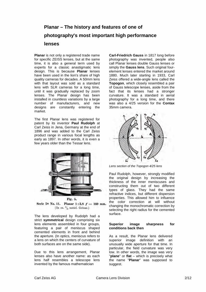
Planar is not only a registered trade name for specific ZEISS lenses, but at the same time, it is also a general term used by experts for a classic anastigmatic lens design. This is because Planar lenses have been used in the lion's share of high quality cameras for decades. A 50mm lens with that layout was sold as a standard lens with SLR cameras for a long time, until it was gradually replaced by zoom lenses. The Planar design has been installed in countless variations by a large number of manufacturers, and new designs are constantly entering the market. The first Planar lens was registered for patent by its inventor Paul Rudolph at Carl Zeiss in Jena, Germany at the end of 1896 and was added to the Carl Zeiss product range in various focal lengths as early as 1897. In other words, it is even a few years older than the Tessar lens.

The lens developed by Rudolph had a strict symmetrical design comprising six lens elements assembled in four groups, featuring a pair of meniscus shaped cemented elements in front and behind the aperture. (In optics, meniscus refers to a lens on which the centers of curvature of both surfaces are on the same side). Due to this lens arrangement, Planar lenses also have another name: as each lens half resembles a telescope lens invented by the famous mathematician

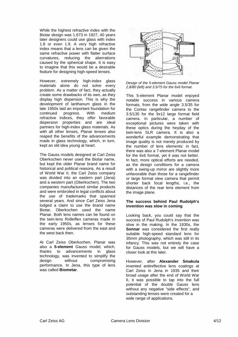
Carl-Friedrich Gauss in 1817 long before photography was invented, people also call Planar lenses double Gauss lenses or simply the Gauss lens. Such original four-element lenses entered the market around 1880. Much later starting in 1933, Carl Zeiss offered a wide-angle lens called the Topogon, which closely resembled a pair of Gauss telescope lenses, aside from the fact that its lenses had a stronger curvature. It was a standard in aerial photography for a long time, and there was also a 4/25 version for the Contax 35mm camera.

Lens section of the Topogon 4/25 lens Paul Rudolph, however, strongly modified the original design by increasing the thickness of the inner meniscuses and constructing them out of two different types of glass. They had the same refractive indices, but different dispersion properties. This allowed him to influence the color correction at will without changing the monochromatic correction by selecting the right radius for the cemented surface. Superior image sharpness for conditions back then As a result, the Planar lens delivered superior image definition with an unusually wide aperture for that time. In particular, the field curvature was very low. In other words, the image was very "plane" or flat – which is precisely what the name "Planar" was supposed to suggest.

Carl Zeiss AG Camera Lens Division 3/12

A catalog from 1897 stated the following: "When working with the Planar, keep in mind that slight overexposures can easily result from the high speed of the lens. The precise design of the Planar lens surpasses the anastigmatic double lenses introduced until now. Above all, it is especially suitable for all kinds of reproductions and yields excellent results." And since chromatic aberrations tend to be more noticeable with line originals, i.e., where the contrast between black and white is high, other models soon incorporated the same design, but featured even better chromatic correction thanks to the use of special types of glass.

Despite all of these favorable features, the Planar lens enjoyed only marginal success in the beginning. Although the older double anastigmatic lenses (later: Protar) were not quite as good, they were slightly more versatile, because the front and rear lens halves could be used alone, therefore allowing three focal lengths with a single lens. This was not possible with the Planar. The Tessar lens, which was offered starting in 1902, achieved very good results in practice and was less expensive. Above all, it was considerably lighter. In particular, the Planar lens was considerably more sensitive to bright light sources in the image due to its eight glass-to-air surfaces and unfavorable curvature. Antireflective lens coatings had not yet been invented. This meant that unwanted optical paths of several reflections in the lens created ghosts and glare in the image, because each glass-to-air surface reflected around 4% of the incident light.

It was not until the 1920s that optic designers resumed efforts to advance the double Gauss lens. Their primary objective was to increase its speed. In 1927, for example, Willy Merté at Carl Zeiss in Jena designed an entire series of lenses for 35mm cameras and 16mm movie film with a maximum aperture of f/2 and f/1.4. These new designs entered the market under the name Biotar. Its design was very similar to the original Planar lens, but it abandoned the strict symmetry approach for the radii of curvature of the surfaces and the refractive indices of the glass materials and therefore achieved additional correction parameters. Virtually all of today's fast lenses are based on the Biotar design Nearly all of today's high-speed lenses with a medium field angle (50-100mm focal length with 35mm SLR cameras) are successors to the Biotar design. The number of variations is virtually endless. To achieve maximum apertures, one or two lenses were added to the classic 6-element lens. The elements were combined into cemented components at a wide range of positions. Despite looking similar on the outside, there are major differences in performance between today's models and their predecessors, improvements which are largely attributable to the development of new glass materials.

The Planar 2/50 ZM – a modern double Gauss lens for a 35mm rangefinder camera.

Carl Zeiss AG Camera Lens Division 4/12

While the highest refractive index with the Biotar design was 1.673 in 1927, 40 years later designers could use glass with index 1.8 or even 1.9. A very high refractive index means that a lens can be given the same refractive power with flatter surface curvatures, reducing the aberrations caused by the spherical shape. It is easy to imagine that this would be a desirable feature for designing high-speed lenses. However, extremely high-index glass materials alone do not solve every problem. As a matter of fact, they actually create some drawbacks of its own, as they display high dispersion. This is why the development of lanthanum glass in the late 1950s laid an important foundation for continued progress. With medium refractive indices, they offer favorable dispersion properties and are ideal partners for high-index glass materials. As with all other lenses, Planar lenses also reaped the benefits of the advancements made in glass technology, which, in turn, kept an old idea young at heart. The Gauss models designed at Carl Zeiss Oberkochen never used the Biotar name, but kept the older Planar brand name for historical and political reasons. As a result of World War II, the Carl Zeiss company was divided into an eastern part (Jena) and a western part (Oberkochen). The two companies manufactured similar products and were embroiled in legal conflicts about the use of trademarks that spanned several years. And since Carl Zeiss Jena lodged a claim to use the brand name Biotar, Oberkochen used the name Planar. Both lens names can be found on the twin-lens Rolleiflex cameras made in the early 1950s, as lenses for these cameras were delivered from the east and the west back then. At Carl Zeiss Oberkochen, Planar was also a 5-element Gauss model, which, thanks to advancements in glass technology, was invented to simplify the design without compromising performance. In Jena, this type of lens was called Biometar.

Design of the 5-element Gauss model Planar 2,8/80 (left) and 3.5/75 for the 6x6 format. This 5-element Planar model enjoyed notable success in various camera formats, from the wide angle 3.5/35 for the Contax rangefinder camera to the 3.5/135 for the 9x12 large format field camera. In particular, a number of exceptional pictures were taken with these optics during the heyday of the twin-lens SLR camera. It is also a wonderful example demonstrating that image quality is not merely produced by the number of lens elements: in fact, there was also a 7-element Planar model for the 6x6 format, yet it was not better. In fact, more optical efforts are needed, as the design conditions for a camera with a swing-up mirror are slightly more unfavorable than those for a rangefinder or large format view camera that permit shorter back focal lengths, i.e., the distances of the rear lens element from the image plane. The success behind Paul Rudolph's invention was slow in coming Looking back, you could say that the success of Paul Rudolph's invention was slow in the making. In the 1930s, the Sonnar was considered the first really suitable high-speed standard lens for 35mm photography, which was still in its infancy. This was not entirely the case for Gauss models, but we will have a closer look at this later. However, after Alexander Smakula invented antireflective lens coatings at Carl Zeiss in Jena in 1935 and their broad usage after the end of World War II, it was possible to tap into the full potential of the double Gauss lens without any negative "side effects", and outstanding lenses were created for a wide range of applications.

Carl Zeiss AG Camera Lens Division 5/12

Planar 0,7/50 – famous for its speed, turned into a movie star thanks to Stanley Kubrick The Planar 0,7/50 from the 1960s is a famous example of the possibilities of this lens type to gain speed and it holds a world record in photography. The lens delivered an image that was four times brighter than with today's standard 1.4/50 lens. It was originally developed on behalf of NASA to take pictures of the dark side of the moon. Its fame skyrocketed when the legendary director Stanley Kubrick pushed the envelope on his quest to give his film "Barry Lyndon" a unique look by insisting on filming several scenes in candlelight. In 2011, one of these lenses was auctioned off for 90,000 euros. Unfortunately, it is practically impossible to adapt this "dream lens" to an SLR camera. It had an image circle diameter of 27mm, making it almost an APS-C, a diameter of around 90mm and weighed in at 1850 grams. And the large lens element diameters had to come very close to the film plane: the distance to the last lens vertex was only 5.3mm. It was therefore fitted with a central shutter for large-format camera optics and was precisely adjusted to a modified HASSELBLAD body.

Design and front lens of the world's fastest camera lens, the Planar 0.7/50

There were also more ‘earthly’ tasks outside of normal photography, which focused on other properties than speed, e.g., uniform definition and the total absence of distortion throughout the image field in microfilm documentation.

S-Orthoplanar for documentation on microfilm in 32x45mm format; MTF for spatial frequencies of 25, 50 and 100 Lp/mm. The radial distortion is less than 0.1%. While these lenses are also excellently suited for macrophotography, this is less the case for other members of the Planar family, which frequently can be found in second-hand markets, e.g., the S-Planar 1,1/42: This is a lens from the early days of microlithography in the semiconductor industry, corrected for the wavelength 436nm only and therefore has a resolving power of much more than 1000 Lp/mm with a depth of focus of 1.2 µm. In other words, it is the wrong choice and practically useless for everyday photography.

Carl Zeiss AG Camera Lens Division 6/12

The patent from 1896 and the basis for emerging models over the decades.

Carl Zeiss AG Camera Lens Division 7/12

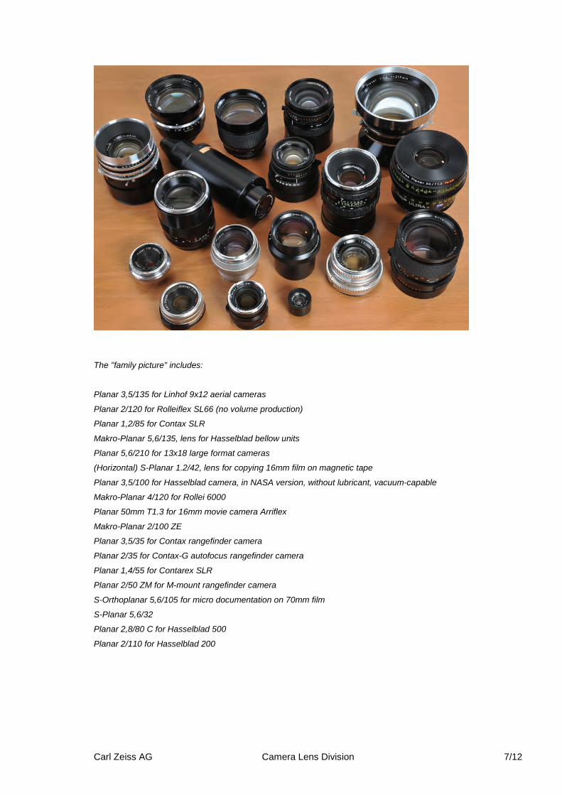
The "family picture" includes: Planar 3,5/135 for Linhof 9x12 aerial cameras

Planar 2/120 for Rolleiflex SL66 (no volume production)

Planar 1,2/85 for Contax SLR

Makro-Planar 5,6/135, lens for Hasselblad bellow units

Planar 5,6/210 for 13x18 large format cameras

(Horizontal) S-Planar 1.2/42, lens for copying 16mm film on magnetic tape

Planar 3,5/100 for Hasselblad camera, in NASA version, without lubricant, vacuum-capable

Makro-Planar 4/120 for Rollei 6000

Planar 50mm T1.3 for 16mm movie camera Arriflex

Makro-Planar 2/100 ZE

Planar 3,5/35 for Contax rangefinder camera

Planar 2/35 for Contax-G autofocus rangefinder camera

Planar 1,4/55 for Contarex SLR

Planar 2/50 ZM for M-mount rangefinder camera

S-Orthoplanar 5,6/105 for micro documentation on 70mm film

S-Planar 5,6/32

Planar 2,8/80 C for Hasselblad 500

Planar 2/110 for Hasselblad 200

Carl Zeiss AG Camera Lens Division 8/12

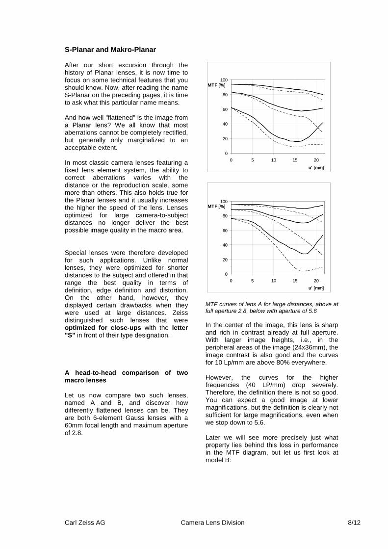
S-Planar and Makro-Planar After our short excursion through the history of Planar lenses, it is now time to focus on some technical features that you should know. Now, after reading the name S-Planar on the preceding pages, it is time to ask what this particular name means. And how well "flattened" is the image from a Planar lens? We all know that most aberrations cannot be completely rectified, but generally only marginalized to an acceptable extent. In most classic camera lenses featuring a fixed lens element system, the ability to correct aberrations varies with the distance or the reproduction scale, some more than others. This also holds true for the Planar lenses and it usually increases the higher the speed of the lens. Lenses optimized for large camera-to-subject distances no longer deliver the best possible image quality in the macro area. Special lenses were therefore developed for such applications. Unlike normal lenses, they were optimized for shorter distances to the subject and offered in that range the best quality in terms of definition, edge definition and distortion. On the other hand, however, they displayed certain drawbacks when they were used at large distances. Zeiss distinguished such lenses that were optimized for close-ups with the letter "S" in front of their type designation. A head-to-head comparison of two macro lenses Let us now compare two such lenses, named A and B, and discover how differently flattened lenses can be. They are both 6-element Gauss lenses with a 60mm focal length and maximum aperture of 2.8.

0

20

40

60

80

100

0 5 10 15 20

u' [mm]

MTF [%]

0

20

40

60

80

100

0 5 10 15 20u' [mm]

MTF [%]

MTF curves of lens A for large distances, above at full aperture 2.8, below with aperture of 5.6 In the center of the image, this lens is sharp and rich in contrast already at full aperture. With larger image heights, i.e., in the peripheral areas of the image (24x36mm), the image contrast is also good and the curves for 10 Lp/mm are above 80% everywhere. However, the curves for the higher frequencies (40 LP/mm) drop severely. Therefore, the definition there is not so good. You can expect a good image at lower magnifications, but the definition is clearly not sufficient for large magnifications, even when we stop down to 5.6. Later we will see more precisely just what property lies behind this loss in performance in the MTF diagram, but let us first look at model B:

Carl Zeiss AG Camera Lens Division 9/12

0

20

40

60

80

100

0 5 10 15 20

u' [mm]

MTF [%]

0

20

40

60

80

100

0 5 10 15 20u' [mm]

MTF [%]

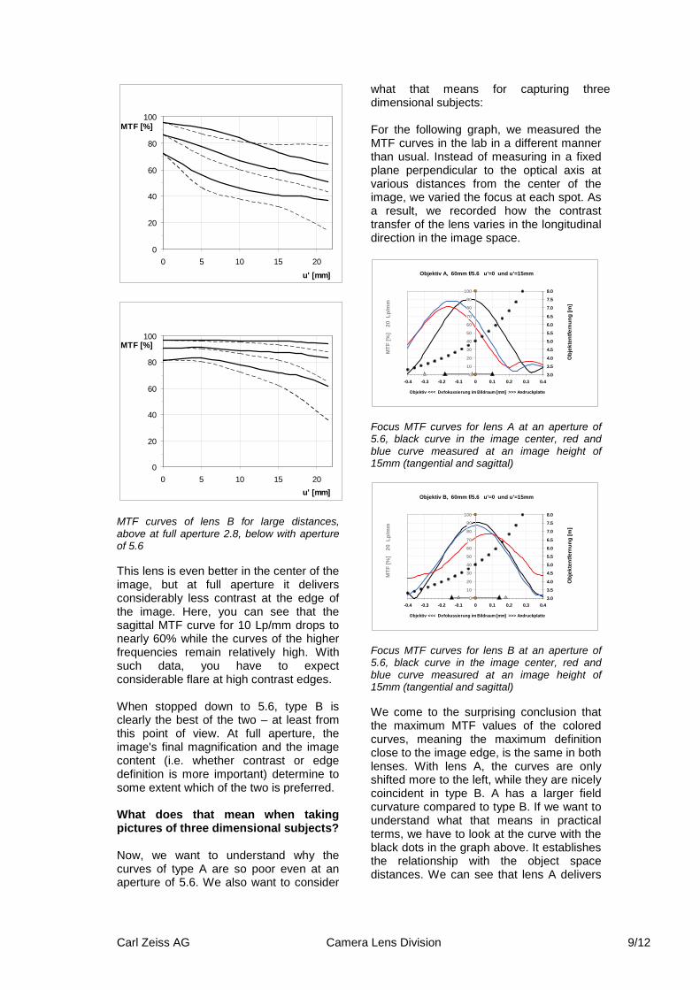
MTF curves of lens B for large distances, above at full aperture 2.8, below with aperture of 5.6 This lens is even better in the center of the image, but at full aperture it delivers considerably less contrast at the edge of the image. Here, you can see that the sagittal MTF curve for 10 Lp/mm drops to nearly 60% while the curves of the higher frequencies remain relatively high. With such data, you have to expect considerable flare at high contrast edges. When stopped down to 5.6, type B is clearly the best of the two – at least from this point of view. At full aperture, the image's final magnification and the image content (i.e. whether contrast or edge definition is more important) determine to some extent which of the two is preferred. What does that mean when taking pictures of three dimensional subjects? Now, we want to understand why the curves of type A are so poor even at an aperture of 5.6. We also want to consider

what that means for capturing three dimensional subjects: For the following graph, we measured the MTF curves in the lab in a different manner than usual. Instead of measuring in a fixed plane perpendicular to the optical axis at various distances from the center of the image, we varied the focus at each spot. As a result, we recorded how the contrast transfer of the lens varies in the longitudinal direction in the image space.

Objektiv A, 60mm f/5.6 u'=0 und u'=15mm

0

10

20

30

40

50

60

70

80

90

100

-0.4 -0.3 -0.2 -0.1 0 0.1 0.2 0.3 0.4

Objektiv <<< Defokussierung im Bildraum [mm] >>> Andruckplatte M

TF [%

] 2

0 L

p/m

m

3.0

3.5

4.0

4.5

5.0

5.5

6.0

6.5

7.0

7.5

8.0

Obj

ekte

ntfe

rnun

g [m

]

Focus MTF curves for lens A at an aperture of 5.6, black curve in the image center, red and blue curve measured at an image height of 15mm (tangential and sagittal)

Objektiv B, 60mm f/5.6 u'=0 und u'=15mm

0

10

20

30

40

50

60

70

80

90

100

-0.4 -0.3 -0.2 -0.1 0 0.1 0.2 0.3 0.4

Objektiv <<< Defokussierung im Bildraum [mm] >>> Andruckplatte

MTF

[%]

20

Lp/

mm

3.0

3.5

4.0

4.5

5.0

5.5

6.0

6.5

7.0

7.5

8.0

Obj

ekte

ntfe

rnun

g [m

]

Focus MTF curves for lens B at an aperture of 5.6, black curve in the image center, red and blue curve measured at an image height of 15mm (tangential and sagittal) We come to the surprising conclusion that the maximum MTF values of the colored curves, meaning the maximum definition close to the image edge, is the same in both lenses. With lens A, the curves are only shifted more to the left, while they are nicely coincident in type B. A has a larger field curvature compared to type B. If we want to understand what that means in practical terms, we have to look at the curve with the black dots in the graph above. It establishes the relationship with the object space distances. We can see that lens A delivers

Carl Zeiss AG Camera Lens Division 10/12

ideal definition at the image edge at approx. 4m if you focus in the center to 5 meters. If we take a picture of an attractive house with an inviting street café in front of it, this curvature can be beneficial, since the foreground is captured with greater definition. If we only want to take a picture of the facade, for example, similar to reproducing a flat image, type B would be the better choice. We would then need to stop down type A to 8 or 11 if we know its properties. Since the world in front of the camera is largely three dimensional, i.e., it has depth, the perfect flattening of lenses is not necessarily always the best solution, especially since the effort required to correct the field curvature, which is limited by volume and cost, must be weighed against other abberations. For example, it often helps to leave the curvature slightly undercorrected to correct the spherical abberation and astigmatism. We see this as a trade-off between the various strengths and weaknesses of our two examples. Comparing both lenses in close-up range with a scale of 1:10 To complete the assessment of the two lenses, we will now compare them in the close-up range at a scale of 1:10. Afterwards, it will be more difficult to determine which lens is "better":

0

20

40

60

80

100

0 5 10 15 20

u' [mm]

MTF [%]

0

20

40

60

80

100

0 5 10 15 20u' [mm]

MTF [%]

MTF curves of lens A in close-up range with a reproduction scale of 1:10, aperture 2.8 (above) and aperture 5.6

0

20

40

60

80

100

0 5 10 15 20

u' [mm]

MTF [%]

0

20

40

60

80

100

0 5 10 15 20u' [mm]

MTF [%]

MTF curves of lens B in close-up range with a reproduction scale of 1:10, aperture 2.8 (above) and aperture 5.6 Now, lens A at full aperture in the entire image field is considerably better and the curvature has disappeared. When slightly stopped down, lens B also achieves a good result, but type A has nearly ideal curves.

Carl Zeiss AG Camera Lens Division 11/12

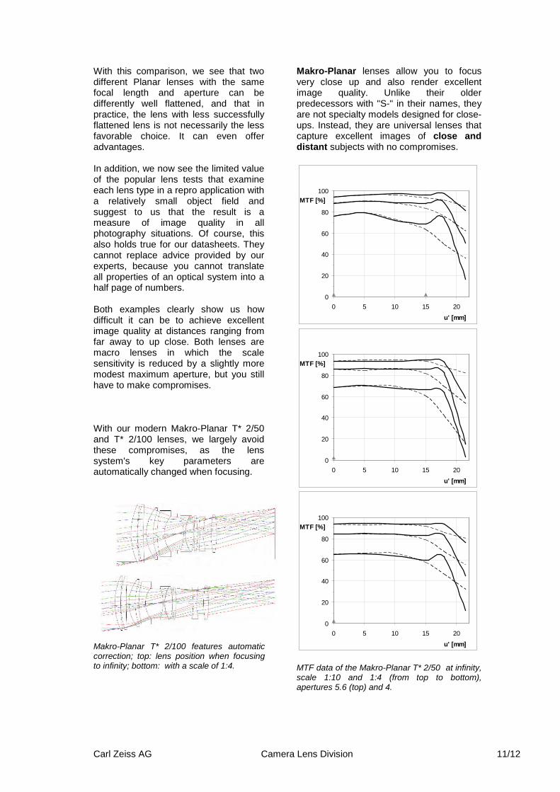
With this comparison, we see that two different Planar lenses with the same focal length and aperture can be differently well flattened, and that in practice, the lens with less successfully flattened lens is not necessarily the less favorable choice. It can even offer advantages. In addition, we now see the limited value of the popular lens tests that examine each lens type in a repro application with a relatively small object field and suggest to us that the result is a measure of image quality in all photography situations. Of course, this also holds true for our datasheets. They cannot replace advice provided by our experts, because you cannot translate all properties of an optical system into a half page of numbers. Both examples clearly show us how difficult it can be to achieve excellent image quality at distances ranging from far away to up close. Both lenses are macro lenses in which the scale sensitivity is reduced by a slightly more modest maximum aperture, but you still have to make compromises. With our modern Makro-Planar T* 2/50 and T* 2/100 lenses, we largely avoid these compromises, as the lens system's key parameters are automatically changed when focusing. Makro-Planar T* 2/100 features automatic correction; top: lens position when focusing to infinity; bottom: with a scale of 1:4.

Makro-Planar lenses allow you to focus very close up and also render excellent image quality. Unlike their older predecessors with "S-" in their names, they are not specialty models designed for close-ups. Instead, they are universal lenses that capture excellent images of close and distant subjects with no compromises.

0

20

40

60

80

100

0 5 10 15 20

u' [mm]

MTF [%]

0

20

40

60

80

100

0 5 10 15 20

u' [mm]

MTF [%]

0

20

40

60

80

100

0 5 10 15 20

u' [mm]

MTF [%]

MTF data of the Makro-Planar T* 2/50 at infinity, scale 1:10 and 1:4 (from top to bottom), apertures 5.6 (top) and 4.

Carl Zeiss AG Camera Lens Division 12/12

Useful Makro accessories: close-up lens, close-up achromats and extension rings Anyone wanting to take close-up shots with his camera for the first time can also capture images below the close-up limits of his lens with the help of affordable accessories. Close-up lenses or achromats, which are screwed into the filter thread and more or less serve the function of eyeglasses for close-up, are the best space-saving accessories and often the best choice for moderate close-ups. With standard lenses with 50mm focal length, they compensate increasing barrel-shaped distortion at short distance. If the close-up lens has a very strong refractive power, however, the system displays a significant amount of blur and flare caused by spherical aberration. This disappears once you stop down, but means you have to adjust your focus. The most reliable option is to focus with a working aperture using Life View.

Extension rings are the accessories which allow you to dive considerably deeper into the close-up range. Here, however, you cannot expect all lenses that are corrected for larger distances to render particularly good image definition with long extensions. Since in macro photography, you normally stop down the aperture further due to desired depth of focus, the definition in the center is sufficient for many subjects, but the corners are not yet really sharp with an aperture of 11. This is why it pays to buy a modern macro lens if you want to take a lot of pictures at a scale of 1:10 or closer. Once you have enjoyed outstanding ease of use and image quality, you will no longer want to do without this versatile tool ever again.

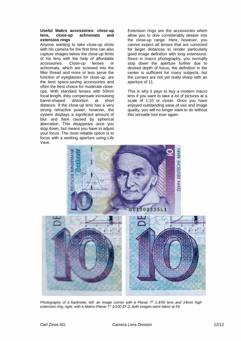
Photography of a banknote, left: an image corner with a Planar T* 1,4/50 lens and 14mm high extension ring, right: with a Makro-Planar T* 2/100 ZF.2, both images were taken at f/4.