From standard reasoning problems to non-standard … · standard reasoning problems to ......
125
From standard reasoning problems to non-standard reasoning problems and one step further Uli Sattler University of Manchester, University of Oslo [email protected]
Transcript of From standard reasoning problems to non-standard … · standard reasoning problems to ......
From standard reasoning problems
to non-standard reasoning problems
andone step further
Uli SattlerUniversity of Manchester, University of [email protected]

Some Advertisement
Some Advertisement
Cover illustration: The Description Logic logo. Courtesy of Enrico Franconi.
Baader, Horrocks,
Lutz, SattlerAn Introduction to D
escription Logic
Description Logics (DLs) have a long tradition in computer science and knowledge representation, being designed so that domain knowledge can be described and so that computers can reason about this knowledge. DLs have recently gained increased importance since they form the logical basis of widely used ontology languages, in particular the web ontology language OWL.
Written by four renowned experts, this is the first textbook on Description Logic. It is suitable for self-study by graduates and as the basis for a university course. Starting from a basic DL, the book introduces the reader to their syntax, semantics, reasoning problems and model theory, and discusses the computational complexity of these reasoning problems and algorithms to solve them. It then explores a variety of reasoning techniques, knowledge-based applications and tools, and describes the relationship between DLs and OWL.
Franz Baader is a professor in the Institute of Theoretical Computer Science at TU Dresden.
Ian Horrocks is a professor in the Department of Computer Science at the University of Oxford.
Carsten Lutz is a professor in the Department of Computer Science at the University of Bremen.
Uli Sattler is a professor in the Information Management Group within the School of Computer Science at the University of Manchester.
Designed by Zoe Naylor.
9780521873611 Baader et al. PPC C M Y
K Description LogicAn Introduction to
Franz BaaderIan Horrocks Carsten Lutz Uli Sattler
Get 20% Discount: For more information, and to order, visit:
www.cambridge.org/9780521695428 and enter the code BAADER2017 at the checkout
An Introduction toDescription Logic
Description logics (DLs) have a long tradition in computer science andknowledge representation, being designed so that domain knowledge canbe described and so that computers can reason about this knowledge. DLshave recently gained increased importance since they form the logical basisof widely used ontology languages, in particular the web ontology languageOWL. Written by four renowned experts, this is the first textbook ondescription logics. It is suitable for self-study by graduates and as the basisfor a university course. Starting from a basic DL, the book introduces thereader to their syntax, semantics, reasoning problems and model theoryand discusses the computational complexity of these reasoning problemsand algorithms to solve them. It then explores a variety of reasoningtechniques, knowledge-based applications and tools and it describes therelationship between DLs and OWL.
on this titleExpires 15 March 2018
Technische Universität, DresdenFranz Baader
University of OxfordIan Horrocks
Universität BremenCarsten Lutz
University of Manchesterand Uli Sattler
1. Introduction; 2. A basic DL; 3. A little bit of model theory; 4. Reasoning in DLs with tableaualgorithms; 5. Complexity; 6. Reasoning in the εL family of Description Logics; 7. Queryanswering; 8. Ontology languages and applications; Appendix A. Description Logicterminology; References; Index.
20% Discount
£59.99 £47.99Discount priceOriginal price
$79.99 $63.99
£29.99 £23.99Discount priceOriginal price
$39.99 $31.99
Hardback 978-0-521-87361-1
Paperback 978-0-521-69542-8
April 2017228 x 152 mm 260pp 30 b/w illus.
Standard &
Non-StandardReasoning Problems

Standard Reasoning Problems
we all know them: given decide/compute
• consistency/satisfiability
• subsumption
• classification
• query answering
• …all only involve entailment checks:
• …possibly many (classification!)
O !α
C,D,O, T ,A, . . .

we all know them: given
•
•
•
•
• …involve finding extreme X such that …
• subset-minimal or • maximally/minimally strong
• …possibly many such Xs
Non-Standard Reasoning Problems
C,D,O, T ,A, . . .
Justsp↵,Oq, PinPointp↵,Oq, . . .matchpC,P,Oq, unifypP1, P2,Oq, . . .x-modp⌃,Oq, . . .
mscpa,Oq, lcspC,D,Oq, . . .
Are
• (conservative) rewritability
• (query) inseparability
also standard reasoning problems?

(Non-)Standard Reasoning: we know how to understand problems: • decidability & computational complexity
– worst case– data– parametrised– …
understand solutions: • soundness, completeness, termination• relations between them• complexity
– see above• practicability
– worst case complexity ≠ best case complexity– amenable to optimisation– empirical evaluation

fact hermit
jfact pellet
101000
10000010000000
101000
10000010000000
Ontology/Reasoner pairs
Num
ber o
f tes
ts "ST"
N*log(N)
N^2
ST
Fig. 7: Subsumption tests carried out in relation to a naive N2 upper bound andan N log(N) upper bound, ordered by N , the number of names in eO (y: log scale).
6.1.6 Discussion
A first answer to Question 1 is that (tableau) subsumption testing does not con-tribute at all to classification time for a substantial number of ontologies. We haveestablished a empirical lower bound for BioPortal ontologies that do not involvesubsumption testing at 46%. This lower bound is even slightly naive because (1)there are most likely a number of ontologies that do not involve tests among theunsuccessfully classified ones and (2) only 33% of all ontology-reasoner pairs in-volved tests. The currently secured lower bound for ontologies actually requiringsubsumption testing lies at 14% (i.e. the 47 out of 330 ontologies for which allfour reasoners triggered a test). Note that, while this might seem like a very lownumber, these might be the 50 or so ontologies in the world that are hard andmatter, and thus worth optimising for. As a side note, the low numbers of tests forHermiT and Pellet can perhaps be explained by their internal alternative deter-ministic engines (for example internal EL-reasoners), see Section 5.1.
It is quite interesting that only 10 out of those 146 ontologies that all rea-soners processed caused at least one reasoner to fire a test—all of which are pureOWL 2 EL. Ontologies of the OWL 2 RL or OWL 2 QL family, or less expressiveontologies, did not cause any reasoner to actually fire a test. This suggests thatfor OWL 2 RL and OWL 2 QL ontologies at the very least, the application ofmodular techniques must be strictly motivated by a di↵erent argument than testavoidance or test easyfication. Another potentially interesting observation is thatontologies involving hard tests generally seem to contain rich role-level modelling,most prominently inverses and role hierarchies.
Subsumption test hardness rarely has a strong impact on classification perfor-mance. According to our threshold of “strong impact” at 40% of the overall classi-fication time, FaCT++ encountered impactful ontologies 7.8% of the time, JFact9.6% of the time, Pellet 4.2% of the time and HermiT only in 3 out of its 284 suc-
An interesting side note from our empirical evaluation: how many subsumption does classification involve?
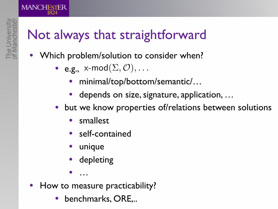
Not always that straightforward• Which problem/solution to consider when?
• e.g., • minimal/top/bottom/semantic/…
• depends on size, signature, application, …
• but we know properties of/relations between solutions
• smallest
• self-contained• unique
• depleting
• …
• How to measure practicability?
• benchmarks, ORE,..
x-modp⌃,Oq, . . .
Extension/variants of DLs
• probabilistic
• non-monotonic
• rules
• …

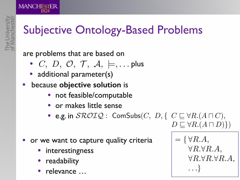
Subjective Ontology-Based Problems

are problems that are based on• plus• additional parameter(s)
Subjective Ontology-Based Problems
C, D, O, T , A, |=, . . .

are problems that are based on• plus• additional parameter(s)
Subjective Ontology-Based Problems
C, D, O, T , A, |=, . . .
SROIQ : ComSubs(C, D, { C v 8R.(A u C),D v 8R.(A uD)})
• because objective solution is • not feasible/computable • or makes little sense• e.g. in

are problems that are based on• plus• additional parameter(s)
Subjective Ontology-Based Problems
C, D, O, T , A, |=, . . .
“ t @R.A,@[email protected],@R.@[email protected],. . .u
SROIQ : ComSubs(C, D, { C v 8R.(A u C),D v 8R.(A uD)})
• because objective solution is • not feasible/computable • or makes little sense• e.g. in
are problems that are based on• plus• additional parameter(s)
Subjective Ontology-Based Problems
C, D, O, T , A, |=, . . .
“ t @R.A,@[email protected],@R.@[email protected],. . .u
• or we want to capture quality criteria• interestingness• readability• relevance …
SROIQ : ComSubs(C, D, { C v 8R.(A u C),D v 8R.(A uD)})
• because objective solution is • not feasible/computable • or makes little sense• e.g. in

A subjective OB problem:Mining TBox Axioms from KBs
or Finding Interesting Correlations

‣ learn (implicit) correlations in our data
‣ get interesting insights into domain
Mining TBox axioms from KBs
TBox
ABox
Learneraxiomaxiomaxiomaxiomaxiom
Do not confuse with (exact) learning of TBoxes (via probing queries)

Mining TBox axioms from KBs
• Correlations in KB = classical machine learning
‣ automatic generation of knowledge from data – taking background knowledge in KB into account– unbiased: let the data speak!– unsupervised (no positive/negative examples)– Semantic Data Mining
TBox
ABox
Learneraxiomaxiomaxiomaxiomaxiom
Hypotheses

Mining TBox axioms from KBs
• Which kind of hypotheses to capture correlations in KB? 1. expressive: GCIs, role inclusions 2. readable3. logically sound4. statistically sound
axiomaxiomaxiomaxiomaxiom
Hypotheses

2. Readable Hypotheses
• A hypothesis is – a small set of short axioms
• fewer than axioms• with concepts shorter than
– in a suitable DL: – free of redundancy
• no superfluous parts ✓preferred laconic justifications
nmax
`max
ALCHI . . .SROIQ
axiomaxiomaxiomaxiomaxiom
Hypotheses

3. Logically Sound Hypotheses
• A hypothesis H should be✓ informative:
✓we want to mine new axioms
✓ consistent: ✓ non-redundant among all hypotheses:
• there is no
8↵ 2 H : O 6|= ↵
O [H 6|= > v ?
axiomaxiomaxiomaxiomaxiom
Hypotheses
H 0, H 2 H : H 6= H 0 and H 0 ⌘ H

3. Logically Sound Hypotheses
• A hypothesis H should be✓ informative:
✓we want to mine new axioms
✓ consistent: ✓ non-redundant among all hypotheses:
• there is no
• Different hypotheses can be compared wrt. their✓ logical strength: ? maximally strong?
• no: overfitting!
? minimally strong? • no: under-fitting
✓ reconciliatory power• brings together terms so
far only loosely related
8↵ 2 H : O 6|= ↵
O [H 6|= > v ?
axiomaxiomaxiomaxiomaxiom
Hypotheses
H 0, H 2 H : H 6= H 0 and H 0 ⌘ H

• we need to assess data support of hypothesis
• introduce metrics that capture quality of an axiom– learn from association rule mining (ARM):
• count individuals that support a GCI– count instances, neg instances, non-instances
• using standard DL semantics, OWA, TBox, entailments,….• no ‘artificial closure’
– make sure you treat a GCI as an axiom and not as a rule• contrapositive!
– coverage, support, …, lift
4. Statistically Sound Hypotheses

Some useful notation:
• •
• relativized:
• projection tables:
4. Statistically Sound Hypotheses
C1 C2 C3 C4 …Ind1 X X X ? …Ind2 0 X X 0 …Ind3 ? ? X ? …Ind4 ? 0 ? ? …… … … … … …
Inst(C,O) := {a | O |= C(a)}UnKnpC,Oq :“ InstpJ,OqzpInstpC,Oq Y Instp C,Oqq
P(C,O) := # Inst(C,O)/# Inst(>,O)
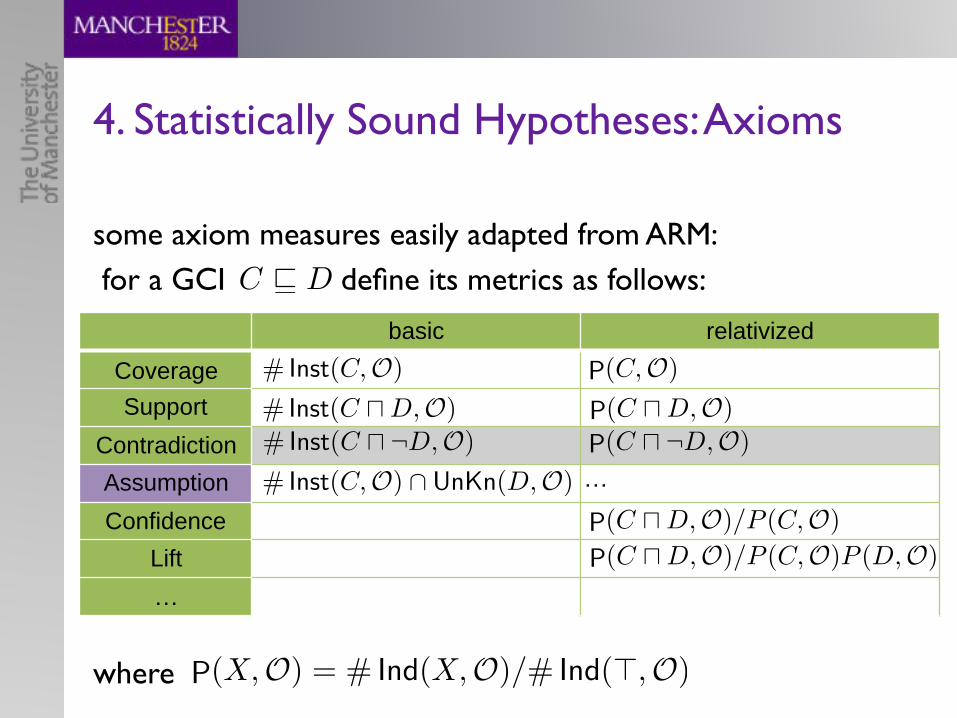
some axiom measures easily adapted from ARM: for a GCI define its metrics as follows:
4. Statistically Sound Hypotheses: Axioms
basic relativized
CoverageSupport
ContradictionAssumption …
ConfidenceLift…
# Inst(C,O)
# Inst(C uD,O)# Inst(C u ¬D,O)
# Inst(C,O) \ UnKn(D,O)
P(C u ¬D,O)P(C uD,O)
P(C,O)
P(C uD,O)/P (C,O)
P(C uD,O)/P (C,O)P (D,O)
where P(X,O) = # Ind(X,O)/# Ind(>,O)
C v D

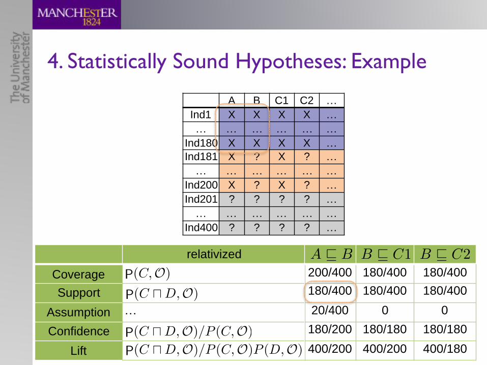
4. Statistically Sound Hypotheses: Example
A B C1 C2 …Ind1 X X X X …… … … … … …
Ind180 X X X X …Ind181 X ? X ? …… … … … … …
Ind200 X ? X ? …Ind201 ? ? ? ? …… … … … … …
Ind400 ? ? ? ? …
relativized
CoverageSupport
Assumption …
ConfidenceLift
P(C uD,O)
P(C,O)
P(C uD,O)/P (C,O)
P(C uD,O)/P (C,O)P (D,O)
200/400 180/400 180/400180/400 180/400 180/40020/400 0 0180/200 180/180 180/180400/200 400/200 400/180
A v B B v C1 B v C2

4. Statistically Sound Hypotheses: Example
A B C1 C2 …Ind1 X X X X …… … … … … …
Ind180 X X X X …Ind181 X ? X ? …… … … … … …
Ind200 X ? X ? …Ind201 ? ? ? ? …… … … … … …
Ind400 ? ? ? ? …
relativized
CoverageSupport
Assumption …
ConfidenceLift
P(C uD,O)
P(C,O)
P(C uD,O)/P (C,O)
P(C uD,O)/P (C,O)P (D,O)
0.5 0.45 0.450.45 0.45 0.450.05 0 00.45 1 1
2 2 2.22
A v B B v C1 B v C2

Oooops!
• make sure we treat GCIs as axioms and not as rules– contrapositive!
• so: turn each GCI into equivalent read below as ‘the resulting LHS’… read below as ‘the resulting RHS’…
4. Statistically Sound Hypotheses: Axioms
X t ¬Y v Y t ¬XX v YC
main relativizedCoverageSupport
ContradictionAssumption …
ConfidenceLift…
# Inst(C,O)
# Inst(C uD,O)# Inst(C u ¬D,O)
# Inst(C,O) \ UnKn(D,O)
P(C u ¬D,O)P(C uD,O)
P(C,O)
P(C uD,O)/P (C,O)
P(C uD,O)/P (C,O)P (D,O)
D

Oooops!
• make sure we treat GCIs as axioms and not as rules– contrapositive!
• so: turn each GCI into equivalent read below as ‘the resulting LHS’… read below as ‘the resulting RHS’…
4. Statistically Sound Hypotheses: Axioms
X t ¬Y v Y t ¬XX v YC
main relativizedCoverageSupport
ContradictionAssumption …
ConfidenceLift…
# Inst(C,O)
# Inst(C uD,O)# Inst(C u ¬D,O)
# Inst(C,O) \ UnKn(D,O)
P(C u ¬D,O)P(C uD,O)
P(C,O)
P(C uD,O)/P (C,O)
P(C uD,O)/P (C,O)P (D,O)
DAxiom measures are semantically faithful,
i.e., Ass(Av B,O) = Ass(¬B v ¬A,O)
Axiom measures are not semantically faithful, e.g.,
S
u
p
p
o
r
t
pA Ñ B,Oq ‰ S
u
p
p
o
r
t
pJ Ñ A \ B,Oq

Goal: mine small sets of (short) axioms
• more readable
- close to what people write
• synergy between axioms should lead to better quality
• how to measure their qualities?
4. Stat. Sound Hypotheses: Sets of Axioms

Goal: learn small sets of (short) axioms
• more readable
- close to what people write
• synergy between axioms should lead to better quality
• how to measure their qualities?• …easy:
1. rewrite set into single axiom as usual2. measure resulting axiom
4. Stat. Sound Hypotheses: Sets of Axioms

H1
Coverage 0.5 0.45 0.45 1 always!Support 0.45 0.45 0.45 0.45 min
Assumption 0.05 0 0 0.55 ?Confidence 0.45 1 1 0.45 support!
Lift 2 2 2.22 1 always!
A v B B v C1 B v C2
H1A B C1 C2 …
Ind1 X X X X …… … … … … …
Ind180 X X X X …Ind181 X ? X ? …… … … … … …
Ind200 X ? X ? …Ind201 ? ? ? ? …… … … … … …
Ind400 ? ? ? ? …
4. Stat. Sound Hypotheses: Sets of Axioms
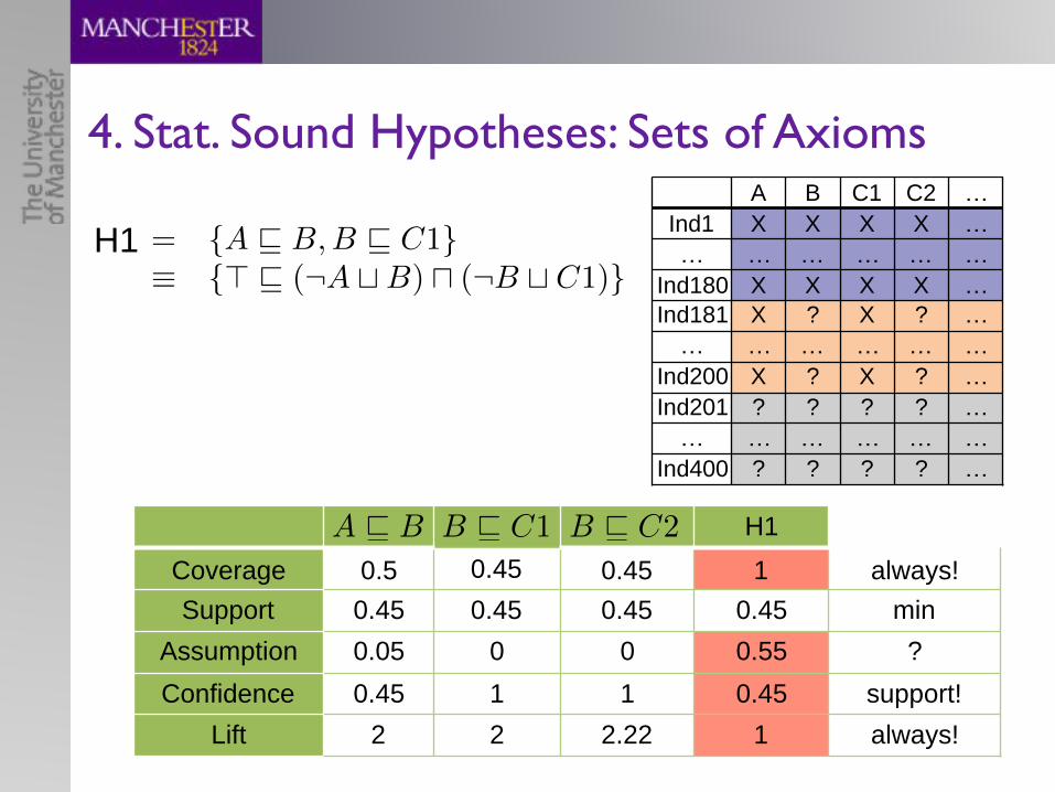
= {A v B,B v C1}⌘ {> v (¬A tB) u (¬B t C1)}
H1
Coverage 0.5 0.45 0.45 1 always!Support 0.45 0.45 0.45 0.45 min
Assumption 0.05 0 0 0.55 ?Confidence 0.45 1 1 0.45 support!
Lift 2 2 2.22 1 always!
A v B B v C1 B v C2
H1A B C1 C2 …
Ind1 X X X X …… … … … … …
Ind180 X X X X …Ind181 X ? X ? …… … … … … …
Ind200 X ? X ? …Ind201 ? ? ? ? …… … … … … …
Ind400 ? ? ? ? …
4. Stat. Sound Hypotheses: Sets of Axioms
= {A v B,B v C1}⌘ {> v (¬A tB) u (¬B t C1)}

Goal: learn small sets of (short) axioms
• more readable
- close to what people write
• synergy between axioms should lead to better quality
• how to measure their qualities?• sum/average quality of their axioms!
4. Stat. Sound Hypotheses: Sets of Axioms

A B C1 C2 …Ind1 X X X X …… … … … … …
Ind180 X X X X …Ind181 X ? X ? …… … … … … …
Ind200 X ? X ? …Ind201 ? ? ? ? …… … … … … …
Ind400 ? ? ? ? …
H1 = {A v B,B v C1}
4. Stat. Sound Hypotheses: Sets of Axioms
H1 H2
Coverage 0.5 0.45 0.45 0.475? 0.475?Support 0.45 0.45 0.45 0.45 0.45
Assumption 0.05 0 0 0.05 0.05Confidence 0.45 1 1 ? ?
Lift 2 2 2.22 ? ?
A v B B v C1 B v C2

A B C1 C2 …Ind1 X X X X …… … … … … …
Ind180 X X X X …Ind181 X ? X ? …… … … … … …
Ind200 X ? X ? …Ind201 ? ? ? ? …… … … … … …
Ind400 ? ? ? ? …
H1 H2
Coverage 0.5 0.45 0.45 0.475? 0.475?Support 0.45 0.45 0.45 0.45 0.45
Assumption 0.05 0 0 0.05 0.05Confidence 0.45 1 1 ? ?
Lift 2 2 2.22 ? ?
A v B B v C1 B v C2
= {A v B,B v C2}H2
H1 = {A v B,B v C1}
4. Stat. Sound Hypotheses: Sets of Axioms

Goal: learn small sets of (short) axioms
• more readable
- close to what people write
• synergy between axioms should lead to better quality
• how to measure their qualities?• observe that a good hypothesis
• allows us to shrink our ABox since it
• captures recurring patterns
• (minimum description length induction)
4. Stat. Sound Hypotheses: Sets of Axioms

Goal: learn small sets of (short) axioms
• more readable
- close to what people write
• synergy between axioms should lead to better quality
• how to measure their qualities?• observe that a good hypothesis
• allows us to shrink our ABox since it
• captures recurring patterns
• use this shrinkage factor to measure a hypothesis’
• fitness - support by data• braveness - number of assumptions
4. Stat. Sound Hypotheses: Sets of Axioms

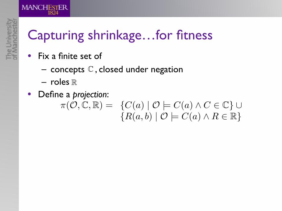
Capturing shrinkage…for fitness• Fix a finite set of
– concepts , closed under negation– roles
CR
Capturing shrinkage…for fitness• Fix a finite set of
– concepts , closed under negation– roles
CR
⇡(O,C,R) = {C(a) | O |= C(a) ^ C 2 C} [{R(a, b) | O |= C(a) ^R 2 R}
• Define a projection:

Capturing shrinkage…for fitness• Fix a finite set of
– concepts , closed under negation– roles
CR
dLen(A,O) = min{`(A0) | A0 [O ⌘ A [O}• For an ABox, define its description length:
⇡(O,C,R) = {C(a) | O |= C(a) ^ C 2 C} [{R(a, b) | O |= C(a) ^R 2 R}
• Define a projection:

Capturing shrinkage…for fitness• Fix a finite set of
– concepts , closed under negation– roles
CR
dLen(A,O) = min{`(A0) | A0 [O ⌘ A [O}• For an ABox, define its description length:
• Define the fitness of a hypothesis H:
fitn(H,O,C,R) = dLen(⇡(O,C,R), T )�dLen(⇡(O,C,R), T [H)
⇡(O,C,R) = {C(a) | O |= C(a) ^ C 2 C} [{R(a, b) | O |= C(a) ^R 2 R}
• Define a projection:

Capturing shrinkage…for braveness
⇡(O,C,R) = {C(a) | O |= C(a) ^ C 2 C} [{R(a, b) | O |= C(a) ^R 2 R}
• Define a projection:
• Fix a finite set of – concepts , closed under negation– roles
CR

Capturing shrinkage…for braveness
• Define a hypothesis’ assumptions: Ass(O, H,C,R) = ⇡(O [H,C,R) \ ⇡(O,C,R)
⇡(O,C,R) = {C(a) | O |= C(a) ^ C 2 C} [{R(a, b) | O |= C(a) ^R 2 R}
• Define a projection:
• Fix a finite set of – concepts , closed under negation– roles
CR

Capturing shrinkage…for braveness
• Define a hypothesis’ assumptions: Ass(O, H,C,R) = ⇡(O [H,C,R) \ ⇡(O,C,R)
• Define the braveness of a hypothesis H:
brave(H,O,C,R) = dLen(Ass(O, H,C,R),O)
⇡(O,C,R) = {C(a) | O |= C(a) ^ C 2 C} [{R(a, b) | O |= C(a) ^R 2 R}
• Define a projection:
Axiom set measures are semantically faithful, i.e.,
H ⌘ H0 ) fitn(H,O,C,R) = fitn(H
0 ,O,C,R)
brave(H,O,C,R) = brave(H
0 ,O,C,R)
• Fix a finite set of – concepts , closed under negation– roles
CR
A B C1 C2Ind1 X X X X… … … … …
Ind180 X X X XInd181 X ? X ?… … … … …
Ind200 X ? X ?Ind201 ? ? ? ?… … … … …
Ind400 ? ? ? ?
= {A v B,B v C2}H2
H1 = {A v B,B v C1}
4. Stat. Sound Hypotheses: Sets of Axioms
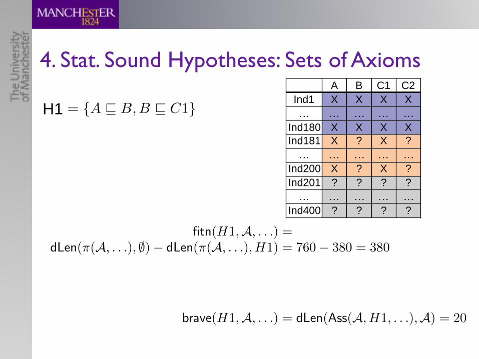
fitn(H1,A, . . .) =dLen(⇡(A, . . .), ;)� dLen(⇡(A, . . .), H1) = 760� 380 = 380
fitn(H2,A, . . .) =dLen(⇡(A, . . .), ;)� dLen(⇡(A, . . .), H2) = 760� 400 = 360
brave(H1,A, . . .) = dLen(Ass(A, H1, . . .),A) = 20
brave(H2,A, . . .) = dLen(Ass(A, H2, . . .),A) = 40

A B C1 C2Ind1 X X X X… … … … …
Ind180 X X X XInd181 X ? X ?… … … … …
Ind200 X ? X ?Ind201 ? ? ? ?… … … … …
Ind400 ? ? ? ?
= {A v B,B v C2}H2
H1 = {A v B,B v C1}
4. Stat. Sound Hypotheses: Sets of Axioms
fitn(H1,A, . . .) =dLen(⇡(A, . . .), ;)� dLen(⇡(A, . . .), H1) = 760� 380 = 380
fitn(H2,A, . . .) =dLen(⇡(A, . . .), ;)� dLen(⇡(A, . . .), H2) = 760� 400 = 360
brave(H1,A, . . .) = dLen(Ass(A, H1, . . .),A) = 20
brave(H2,A, . . .) = dLen(Ass(A, H2, . . .),A) = 40
H1 >> H2

Example: empty TBox, ABox
XA, BA, CA, C
RR
A, CRB
R
A4. Stat. Sound Hypotheses: Sets of Axioms
fitn({X v 8R.A},A, . . .) = dLen(⇡(A, . . .), ;)�dLen(⇡(A, . . .), {X v 8R.A})
= 12� 9= 3
brave({X v 8R.A},A, . . .) = dLen(Ass(A, {X v 8R.A}, . . .),A)= 1

Example: empty TBox, ABox
XA, BA, CA, C
RR
A, CRB
R
A4. Stat. Sound Hypotheses: Sets of Axioms
fitn({X v 8R.A},A, . . .) = dLen(⇡(A, . . .), ;)�dLen(⇡(A, . . .), {X v 8R.A})
= 12� 9= 3
brave({X v 8R.A},A, . . .) = dLen(Ass(A, {X v 8R.A}, . . .),A)= 1

Example: empty TBox, ABox
XA, BA, CA, C
RR
A, CRB
R
A4. Stat. Sound Hypotheses: Sets of Axioms
fitn({X v 8R.A},A, . . .) = dLen(⇡(A, . . .), ;)�dLen(⇡(A, . . .), {X v 8R.A})
= 12� 9= 3
brave({X v 8R.A},A, . . .) = dLen(Ass(A, {X v 8R.A}, . . .),A)= 1

phew…
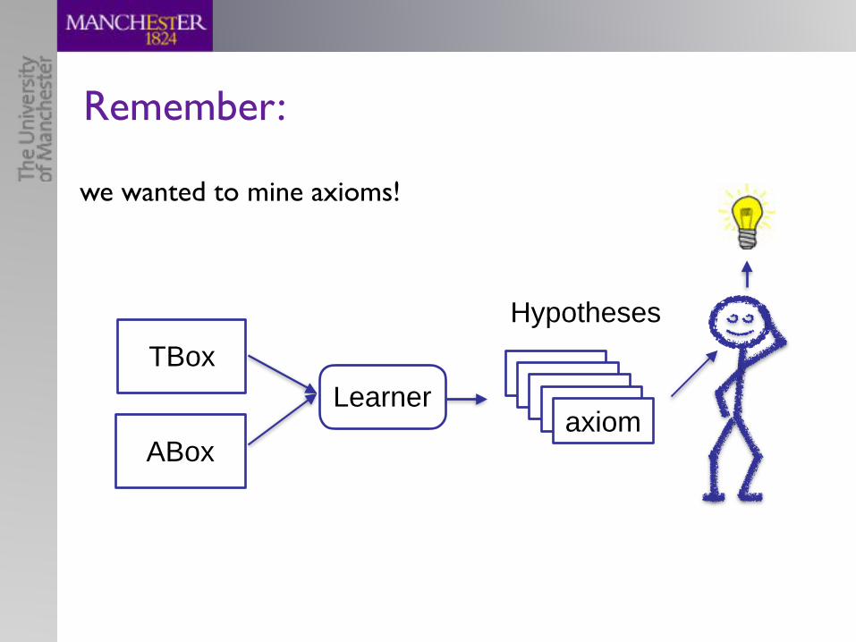
Remember:
TBox
ABox
Learneraxiomaxiomaxiomaxiomaxiom
Hypotheses
we wanted to mine axioms!

H ⌘ H 0 ) fitn(O, H,C,R) = fitn(O, H 0,C,R)
• (Sets of) axioms as Hypotheses
• Loads of measures to capture 1. axiom hypothesis’ coverage, support, assumption, lift, …2. set of axioms hypothesis fitness, braveness
• with a focus of a concept/role spaces ,
• What are their properties? – semantically faithful: …
• Can we compute these measure?– easy for (1), tricky for (2):
So, what have we got?
C R
dLen(A,O) = min{`(A0) | A0 [O ⌘ A [O}
O |= H ) Ass(O, H,C,R) = 0TBox
ABox
Learner
Hypotheses
axiom(s) m1,m2,m3,…axiom(s) m1,m2,m3,…axiom(s) m1,m2,m3,…axiom(s) m1,m2,m3,…axiom(s) m1,m2,m3,…
?
?

H ⌘ H 0 ) fitn(O, H,C,R) = fitn(O, H 0,C,R)
• (Sets of) axioms as Hypotheses
• Loads of measures to capture 1. axiom hypothesis’ coverage, support, assumption, lift, …2. set of axioms hypothesis fitness, braveness
• with a focus of a concept/role spaces ,
• What are their properties? – semantically faithful: …
• Can we compute these measure?– easy for (1), tricky for (2):
So, what have we got?
C R
dLen(A,O) = min{`(A0) | A0 [O ⌘ A [O}
O |= H ) Ass(O, H,C,R) = 0

So, what have we got? (2)
• If we can compute measure, how feasible is this?
• If “feasible”, – do these measures correlate? – how independent are they?
• For which DLs & inputs can we create & evaluate hypotheses?
• Which measures indicate interesting hypothesis?
• What is the shape for interesting hypothesis? – are longer/bigger hypotheses better?
• What do we do with them? – how do we guide users through these?

Slava implements: DL Miner4.2. DESIGNING DL-MINER 75
Ontology CleanerO
Hypothesis ConstructorL, ⌃
Hypothesis EvaluatorQ
Hypothesis Sorter rf(H)
H
qf(H, q)
DL-Miner
Figure 4.1: Architecture of DL-Miner
• Hypothesis Sorter, given the quality function qf(·),3 orders hypothesesH according to the binary relation �.4 The result is the ranking functionrf(H) that returns the quality rank of a hypothesis H 2 H.
The output of DL-Miner is a set H of hypotheses, quality function qf(·), andranking function rf(·). Domain experts and ontology engineers are supposed tonavigate through the hypotheses using the quality and ranking functions. Thus,all hypotheses can be methodically examined. Clearly, it is possible to select onlybest hypotheses if necessary. As the reader will find in the following, hypothesesof DL-Miner can, in fact, be used for various purposes and in different scenarios.
In the following, we clarify the parameters and unfold the functionality of eachblock. Hypothesis Evaluator is covered in Chapter 5, where we define qualitymeasures that can be used in Q, and Chapter 6, where we develop techniquesto compute those measures. Hypothesis Constructor is explained in Chapter 7where we show how to construct suitable concepts C (roles R) given a languagebias L and generate hypotheses H from C (R). Ontology Cleaner and HypothesisSorter are both covered in Chapter 8 where we also integrate all techniques inDL-Miner. Finally, we empirically evaluate DL-Miner in Chapter 9.
3The symbol “ ·” stands for the arguments of the function if they are clear or irrelevant.4When O and Q are clear from the context, we denote the binary relation �O,Q by �.
TBox
ABox
axiom( m1,m2,m3axiom( m1,m2,m3axiom( m1,m2,m3axiom( m1,m2,m3axiom(s) m1,m2,m3,…
parameters
Subjective Solution

Easy:
• construct all concepts C1, C2, …– finitely many thanks to language bias
• check for each whether it’s logically ok: – –
if yes, add it to• remove redundant hypotheses from H
DL Miner: Hypothesis Constructor
LCi v Cj
O [ {Ci v Cj} 6|= > v ?O 6|= Ci v Cj
H

Easy:
• construct all concepts C1, C2, …– finitely many thanks to language bias
• check for each whether it’s logically ok: – –
if yes, add it to• remove redundant hypotheses from H
DL Miner: Hypothesis Constructor
LCi v Cj
O [ {Ci v Cj} 6|= > v ?O 6|= Ci v Cj
H
Bonkers!
Even for EL,
100 concept/role names
4 max length of concepts Ci
~100,000,000 concepts Ci
~100,000,0002 GCIs to test
Bonkers!
Even for EL,
n concept/role names
k max length of concepts Ci
nk concepts Ci
n2k GCIs to test

Use a refinement operator to build Ci informed by ABox– used in concept learning, conceptual blending
• Given a logic , define a refinement operator as – a function such that,
for each
• A refinement operator is
– proper if, for all
– complete if, for all
– suitable if, for all
DL Miner: Hypothesis Constructor
L⇢ : Conc(L) 7! P(Conc(L))
C 2 L, C 0 2 ⇢(C) : C 0 v C
C 2 L, C 0 2 ⇢(C) : C 0 6⌘ C
C P L there is n,C 1 P ⇢npJq : C 1 ” C and`pC 1q § `pCq
C,C 1 P L : if C 1 à Cthen there is some n,C2 ” Cwith C 1 P ⇢npC2q

Use a refinement operator to build Ci informed by ABox– used in concept learning, conceptual blending
• Given a logic , define a refinement operator as – a function such that,
for each
• A refinement operator is
– proper if, for all
– complete if, for all
– suitable if, for all
DL Miner: Hypothesis Constructor
L⇢ : Conc(L) 7! P(Conc(L))
C 2 L, C 0 2 ⇢(C) : C 0 v C
C 2 L, C 0 2 ⇢(C) : C 0 6⌘ C
C P L there is n,C 1 P ⇢npJq : C 1 ” C and`pC 1q § `pCq
Great: there are known refinement
operators (proper, complete, suitable,…)
for ALC [LehmHitzler2010]
C,C 1 P L : if C 1 à Cthen there is some n,C2 ” Cwith C 1 P ⇢npC2q

DL Miner: Concept Constructor7.3. BOTTOM-UP CONSTRUCTION 155
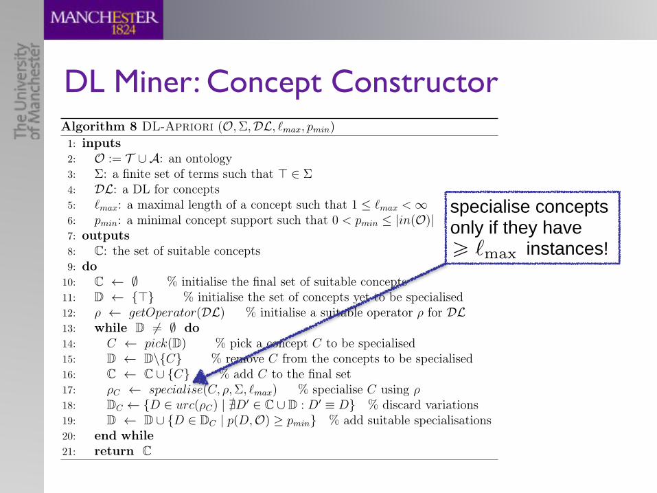
Algorithm 8 DL-Apriori (O,⌃,DL, `max, pmin)1: inputs2: O := T [A: an ontology3: ⌃: a finite set of terms such that > 2 ⌃4: DL: a DL for concepts5: `max: a maximal length of a concept such that 1 `max <16: pmin: a minimal concept support such that 0 < pmin |in(O)|7: outputs8: C: the set of suitable concepts9: do
10: C ; % initialise the final set of suitable concepts11: D {>} % initialise the set of concepts yet to be specialised12: ⇢ getOperator(DL) % initialise a suitable operator ⇢ for DL13: while D 6= ; do14: C pick(D) % pick a concept C to be specialised15: D D\{C} % remove C from the concepts to be specialised16: C C [ {C} % add C to the final set17: ⇢C specialise(C, ⇢,⌃, `max) % specialise C using ⇢18: DC {D 2 urc(⇢C) | @D0 2 C [ D : D0 ⌘ D} % discard variations19: D D [ {D 2 DC | p(D,O) � pmin} % add suitable specialisations20: end while21: return C
the respective specialised concept. The construction begins from the root node >.It repeatedly specialises every leaf node which satisfies the restrictions and is nota syntactic variation. Once there is no such leaf node, the algorithm terminates.All nodes, except leaf nodes, of the constructed tree constitute the final set ofsuitable concepts. Example 7.4 illustrates the bottom-up concept constructionusing DL-Apriori.
Example 7.4. Consider the ontology O used in Example 3.1.
O := {Man v ¬Woman, hasParent v hasChild�,
Man(Arthur), Man(Chris), Man(James),
Woman(Penelope), Woman(V ictoria),
Woman(Charlotte), Woman(Margaret),
hasParent(Charlotte, James), hasParent(Charlotte, V ictoria),
hasParent(V ictoria, Chris), hasParent(V ictoria, Penelope)
hasParent(Arthur, Penelope), hasParent(Arthur, Chris)}.
DL Miner: Concept Constructor7.3. BOTTOM-UP CONSTRUCTION 155
Algorithm 8 DL-Apriori (O,⌃,DL, `max, pmin)1: inputs2: O := T [A: an ontology3: ⌃: a finite set of terms such that > 2 ⌃4: DL: a DL for concepts5: `max: a maximal length of a concept such that 1 `max <16: pmin: a minimal concept support such that 0 < pmin |in(O)|7: outputs8: C: the set of suitable concepts9: do
10: C ; % initialise the final set of suitable concepts11: D {>} % initialise the set of concepts yet to be specialised12: ⇢ getOperator(DL) % initialise a suitable operator ⇢ for DL13: while D 6= ; do14: C pick(D) % pick a concept C to be specialised15: D D\{C} % remove C from the concepts to be specialised16: C C [ {C} % add C to the final set17: ⇢C specialise(C, ⇢,⌃, `max) % specialise C using ⇢18: DC {D 2 urc(⇢C) | @D0 2 C [ D : D0 ⌘ D} % discard variations19: D D [ {D 2 DC | p(D,O) � pmin} % add suitable specialisations20: end while21: return C
the respective specialised concept. The construction begins from the root node >.It repeatedly specialises every leaf node which satisfies the restrictions and is nota syntactic variation. Once there is no such leaf node, the algorithm terminates.All nodes, except leaf nodes, of the constructed tree constitute the final set ofsuitable concepts. Example 7.4 illustrates the bottom-up concept constructionusing DL-Apriori.
Example 7.4. Consider the ontology O used in Example 3.1.
O := {Man v ¬Woman, hasParent v hasChild�,
Man(Arthur), Man(Chris), Man(James),
Woman(Penelope), Woman(V ictoria),
Woman(Charlotte), Woman(Margaret),
hasParent(Charlotte, James), hasParent(Charlotte, V ictoria),
hasParent(V ictoria, Chris), hasParent(V ictoria, Penelope)
hasParent(Arthur, Penelope), hasParent(Arthur, Chris)}.
specialise concepts only if they have instances! • `
max
Don’t even construct most of the nk concepts Ci

Slava implements: DL Miner4.2. DESIGNING DL-MINER 75
Ontology CleanerO
Hypothesis ConstructorL, ⌃
Hypothesis EvaluatorQ
Hypothesis Sorter rf(H)
H
qf(H, q)
DL-Miner
Figure 4.1: Architecture of DL-Miner
• Hypothesis Sorter, given the quality function qf(·),3 orders hypothesesH according to the binary relation �.4 The result is the ranking functionrf(H) that returns the quality rank of a hypothesis H 2 H.
The output of DL-Miner is a set H of hypotheses, quality function qf(·), andranking function rf(·). Domain experts and ontology engineers are supposed tonavigate through the hypotheses using the quality and ranking functions. Thus,all hypotheses can be methodically examined. Clearly, it is possible to select onlybest hypotheses if necessary. As the reader will find in the following, hypothesesof DL-Miner can, in fact, be used for various purposes and in different scenarios.
In the following, we clarify the parameters and unfold the functionality of eachblock. Hypothesis Evaluator is covered in Chapter 5, where we define qualitymeasures that can be used in Q, and Chapter 6, where we develop techniquesto compute those measures. Hypothesis Constructor is explained in Chapter 7where we show how to construct suitable concepts C (roles R) given a languagebias L and generate hypotheses H from C (R). Ontology Cleaner and HypothesisSorter are both covered in Chapter 8 where we also integrate all techniques inDL-Miner. Finally, we empirically evaluate DL-Miner in Chapter 9.
3The symbol “ ·” stands for the arguments of the function if they are clear or irrelevant.4When O and Q are clear from the context, we denote the binary relation �O,Q by �.
TBox
ABox
axiom( m1,m2,m3axiom( m1,m2,m3axiom( m1,m2,m3axiom( m1,m2,m3axiom(s) m1,m2,m3,…
parameters
8.3. PUTTING ALL THE PIECES TOGETHER: DL-MINER 173
repairOntology(·)O
DL-Apriori (·)buildRolesTopDown(·)generateHypotheses(·)
L, ⌃
evaluateHypotheses(·)Q
rankHypotheses(·) rf(·)
H
qf(·)
DL-Miner
Figure 8.3: Architecture of DL-Miner with subroutines
Another property of Algorithm 11 is that it always terminates. This ensuresthat the algorithm returns an output (even though it may take long) for any legalinput parameters, i.e. satisfying the respective constraints of Algorithm 11. Theproperties of correctness, completeness, and termination of Algorithm 11 followfrom the same properties of its subroutines, see Theorem 8.1.
Theorem 8.1 (Correctness, completeness, termination). Let O, ⌃, L := (DL,`max, pmin, GR, n), Q be legal parameters of DL-Miner. Let (i) – (iii) be thefollowing conditions for a hypothesis H:
(i) H conforms to L;
(ii) H is in NNF;
(iii) eH ✓ ⌃.
Then, all following properties hold for DL-Miner:
• it terminates;
• it is correct: it returns a set H of hypotheses such that H 2 H implies H
satisfies (i) – (iii);
Complete (for the parameters provided).
DL Miner: Hypothesis Evaluator
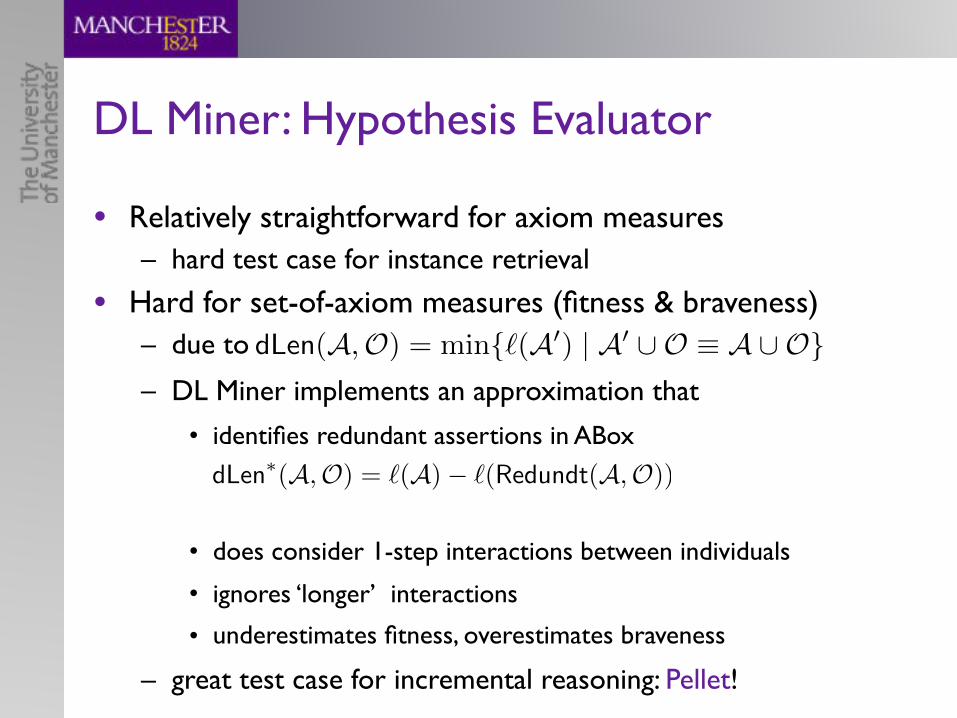
• Relatively straightforward for axiom measures– hard test case for instance retrieval
• Hard for set-of-axiom measures (fitness & braveness)– due to
– DL Miner implements an approximation that
• identifies redundant assertions in ABox
• does consider 1-step interactions between individuals
• ignores ‘longer’ interactions
• underestimates fitness, overestimates braveness
– great test case for incremental reasoning: Pellet!
dLen(A,O) = min{`(A0) | A0 [O ⌘ A [O}
dLen⇤(A,O) = `(A)� `(Redundt(A,O))

DL Miner: Hypothesis Sorter
• Last step in DL Miner’s workflow
• Easy: – throw away all hypotheses that are dominated by another one– i.e., compute the Pareto front wrt the measures provided

DL Miner: Example 176 CHAPTER 8. DL-MINER: A HYPOTHESIS MINING ALGORITHM
Given these input parameters, DL-Miner mines 536 hypotheses whose con-fidence exceeds 0.9. The following are some examples of them:
Woman u 9hasChild.> v Mother (H1)
Man u 9hasChild.> v Father (H2)
9hasChild.> v 9marriedTo.> (H3)
9marriedTo.> v 9hasChild.> (H4)
9marriedTo.Woman v Man (H5)
9marriedTo.Mother v Father (H6)
Father v 9marriedTo.(9hasChild.>) (H7)
Mother v 9marriedTo.(9hasChild.>) (H8)
9hasChild.> v Mother t Father (H9)
9hasChild.> v Man tWoman (H10)
9hasChild.> v Father tWoman (H11)
The hypotheses H1 and H2 provide descriptions for Mother and Father.The hypotheses H3 and H4 indicate interesting correlations in the data: beingmarried implies having children and vice versa. The hypotheses H1, H2, H3, H4
are already discussed in Chapter 3, as they can be obtained by other approaches.In addition to these hypotheses, DL-Miner acquires the hypotheses H5, H6,H7, H8, H9, H10, H11 (and many others) due to the flexible language bias. Thehypothesis H5 provides a description for Man, while the hypotheses H6 – H9
encode additional knowledge about Father and Mother.
The hypotheses H10 and H11 show some issues that can arise while mining hy-potheses using DL-Miner. More specifically, the hypothesis H10 seems carryingno useful knowledge in comparison to H9. The reason is that the input onto-logy Kinship (its TBox) does not capture that everyone is either a man or woman,i.e. Kinship 6|= > v Man tWoman. If the ontology captured this information, thehypothesis H9 would be uninformative and would not be mined (as DL-Minerreturns only informative hypotheses by default). On the other hand, the hypo-thesis H11 seems to be superfluous given H9 since Kinship |= Mother v Woman.Thus, acquired hypotheses can appear to be superfluous due to a poor inputTBox and due to other hypotheses considered in the context of the given TBox.
Given a Kinship Ontology,1 it mines 536 Hs with confidence above 0.9, e.g.
TBox
ABox
DL Miner
1. adapted from UCI Machine Learning Repository

DL Miner: Example 176 CHAPTER 8. DL-MINER: A HYPOTHESIS MINING ALGORITHM
Given these input parameters, DL-Miner mines 536 hypotheses whose con-fidence exceeds 0.9. The following are some examples of them:
Woman u 9hasChild.> v Mother (H1)
Man u 9hasChild.> v Father (H2)
9hasChild.> v 9marriedTo.> (H3)
9marriedTo.> v 9hasChild.> (H4)
9marriedTo.Woman v Man (H5)
9marriedTo.Mother v Father (H6)
Father v 9marriedTo.(9hasChild.>) (H7)
Mother v 9marriedTo.(9hasChild.>) (H8)
9hasChild.> v Mother t Father (H9)
9hasChild.> v Man tWoman (H10)
9hasChild.> v Father tWoman (H11)
The hypotheses H1 and H2 provide descriptions for Mother and Father.The hypotheses H3 and H4 indicate interesting correlations in the data: beingmarried implies having children and vice versa. The hypotheses H1, H2, H3, H4
are already discussed in Chapter 3, as they can be obtained by other approaches.In addition to these hypotheses, DL-Miner acquires the hypotheses H5, H6,H7, H8, H9, H10, H11 (and many others) due to the flexible language bias. Thehypothesis H5 provides a description for Man, while the hypotheses H6 – H9
encode additional knowledge about Father and Mother.
The hypotheses H10 and H11 show some issues that can arise while mining hy-potheses using DL-Miner. More specifically, the hypothesis H10 seems carryingno useful knowledge in comparison to H9. The reason is that the input onto-logy Kinship (its TBox) does not capture that everyone is either a man or woman,i.e. Kinship 6|= > v Man tWoman. If the ontology captured this information, thehypothesis H9 would be uninformative and would not be mined (as DL-Minerreturns only informative hypotheses by default). On the other hand, the hypo-thesis H11 seems to be superfluous given H9 since Kinship |= Mother v Woman.Thus, acquired hypotheses can appear to be superfluous due to a poor inputTBox and due to other hypotheses considered in the context of the given TBox.
Given a Kinship Ontology,1 it mines 536 Hs with confidence above 0.9, e.g.
TBox
ABox
DL MinerGreat - it works really well
on a toy ontology!
1. adapted from UCI Machine Learning Repository

Still: many open questions
• If we can compute measure, how feasible is this?
• If “feasible”, – do these measures correlate? – how independent are they?
• For which DLs & inputs can we create & evaluate hypotheses?
• Which measures indicate interesting hypothesis?
• What is the shape of interesting hypothesis? – are longer/bigger hypotheses better?
• What do we do with them? – how do we guide users through these?
Design, run, analyse experiments

Design, run, analyse experiments
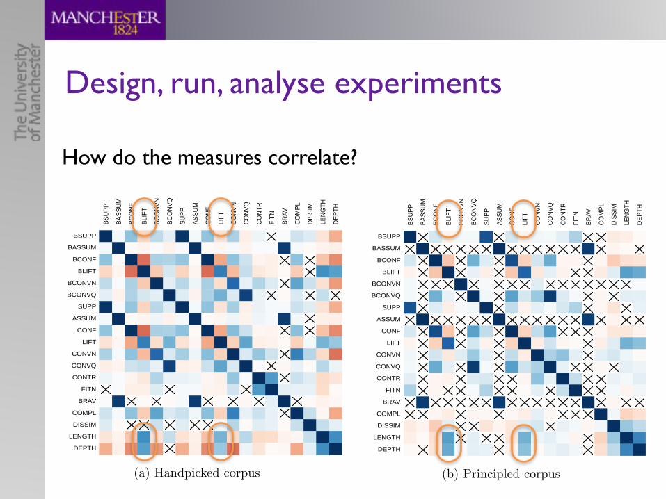
• A corpus - or two:1. handpicked corpus from related work: 16 ontologies2. principled one:
• All BioPortal ontologies with >= 100 individuals and >= 100 RAs 21 ontologies

Design, run, analyse experiments
• A corpus - or two:1. handpicked corpus from related work: 16 ontologies2. principled one:
• All BioPortal ontologies with >= 100 individuals and >= 100 RAs 21 ontologies
• Settings for hypothesis parameters: – is SHI
– RIAs with inverse, composition
– minsupport = 10– max concept length in GCIs = 4
L

Design, run, analyse experiments
• A corpus - or two:1. handpicked corpus from related work: 16 ontologies2. principled one:
• All BioPortal ontologies with >= 100 individuals and >= 100 RAs 21 ontologies
• Settings for hypothesis parameters: – is SHI
– RIAs with inverse, composition
– minsupport = 10– max concept length in GCIs = 4
• generate & evaluate up to 500 hypotheses per ontology
L

Design, run, analyse experiments
• What kind of axioms do people write? – re. readability of hypotheses:– what kind of axioms should we roughly aim for?
9.1. EXPERIMENTAL DATA 185
they constitute ⇡ 25% of the corpus, it is considerably biased towards easy on-tologies. To make the analysis more rigorous, we exclude all ontologies which donot use complex concepts from the results. Thus, 248 ontologies are retained.We gather all axioms of those ontologies, which results in 9,133,219 axioms intotal, and extract their metrics. Table 9.1 shows the proportion of axioms usinga particular DL constructor.
DL constructor C 9R.C C uD 8R.C C tD ¬CAxioms, % 99.73 67.82 1.15 0.46 0.09 0.01
Table 9.1: Use of DL constructors by axioms in BioPortal (ontologies withoutcomplex concepts are excluded)
According to Table 9.1, 99.73% of axioms are concept inclusions. Hence, allrole inclusions constitute just 0.27% of axioms. GCIs constitute around 69% ofaxioms. Interestingly, almost all of them, 98.2%, use existential restrictions thatoccur in 67.82% of axioms overall. This is much more than all other construct-ors (in descending order): conjunctions occur in 1.15%, universal restrictions in0.46%, disjunctions in 0.09%, negations in 0.01% of all axioms. In addition,disjointness axioms, which constitute 1.22% of all axioms, augment the fractionof conjunctions, if interpreted as C u D v ?, or the fraction of negations, ifinterpreted as C v ¬D.2
While Table 9.1 shows how frequently common DL constructors are usedin the axioms, it does not show how complex the axioms are. To investigatethis, we measure the length and depth of the axioms using Definition 5.1 andDefinition 5.3, respectively. In particular, we compare the proportions of shortand long axioms, the proportions of shallow and deep axioms, see Table 9.2.
mean mode 5% 25% 50% 75% 95% 99% 99.9%length 2.63 3 2 2 3 3 3 3 5depth 0.69 1 0 0 1 1 1 1 3
Table 9.2: Length and role depth of axioms in BioPortal (ontologies withoutcomplex concepts are excluded)
In Table 9.2 mean and mode are the standard statistical notions which arecalculated across all gathered axioms. For length, the mean is 2.63 and mode is
2In the OWL API disjointness axioms are handled not as concept inclusions, but as a separatetype of axioms.
Length & role depth of axioms in Bioportal - Taxonomies
9.1. EXPERIMENTAL DATA 185
they constitute ⇡ 25% of the corpus, it is considerably biased towards easy on-tologies. To make the analysis more rigorous, we exclude all ontologies which donot use complex concepts from the results. Thus, 248 ontologies are retained.We gather all axioms of those ontologies, which results in 9,133,219 axioms intotal, and extract their metrics. Table 9.1 shows the proportion of axioms usinga particular DL constructor.
DL constructor C 9R.C C uD 8R.C C tD ¬CAxioms, % 99.73 67.82 1.15 0.46 0.09 0.01
Table 9.1: Use of DL constructors by axioms in BioPortal (ontologies withoutcomplex concepts are excluded)
According to Table 9.1, 99.73% of axioms are concept inclusions. Hence, allrole inclusions constitute just 0.27% of axioms. GCIs constitute around 69% ofaxioms. Interestingly, almost all of them, 98.2%, use existential restrictions thatoccur in 67.82% of axioms overall. This is much more than all other construct-ors (in descending order): conjunctions occur in 1.15%, universal restrictions in0.46%, disjunctions in 0.09%, negations in 0.01% of all axioms. In addition,disjointness axioms, which constitute 1.22% of all axioms, augment the fractionof conjunctions, if interpreted as C u D v ?, or the fraction of negations, ifinterpreted as C v ¬D.2
While Table 9.1 shows how frequently common DL constructors are usedin the axioms, it does not show how complex the axioms are. To investigatethis, we measure the length and depth of the axioms using Definition 5.1 andDefinition 5.3, respectively. In particular, we compare the proportions of shortand long axioms, the proportions of shallow and deep axioms, see Table 9.2.
mean mode 5% 25% 50% 75% 95% 99% 99.9%length 2.63 3 2 2 3 3 3 3 5depth 0.69 1 0 0 1 1 1 1 3
Table 9.2: Length and role depth of axioms in BioPortal (ontologies withoutcomplex concepts are excluded)
In Table 9.2 mean and mode are the standard statistical notions which arecalculated across all gathered axioms. For length, the mean is 2.63 and mode is
2In the OWL API disjointness axioms are handled not as concept inclusions, but as a separatetype of axioms.
Use of DL constructors in Bioportal - Taxonomies
Restricting length of
concepts in axioms to 4 (axioms to 8)
is fine!

How do the measures correlate?
Design, run, analyse experiments9.2. EVALUATING QUALITY MEASURES AND PERFORMANCE 193
−1
−0.8
−0.6
−0.4
−0.2
0
0.2
0.4
0.6
0.8
1
BSUP
P
BASS
UM
BCON
F
BLIF
T
BCON
VN
BCON
VQ
SUPP
ASSU
M
CONF
LIFT
CONV
N
CONV
Q
CONT
R
FITN
BRAV
COM
PL
DISS
IM
LENG
TH
DEPT
H
BSUPP
BASSUM
BCONF
BLIFT
BCONVN
BCONVQ
SUPP
ASSUM
CONF
LIFT
CONVN
CONVQ
CONTR
FITN
BRAV
COMPL
DISSIM
LENGTH
DEPTH
(a) Handpicked corpus
−1
−0.8
−0.6
−0.4
−0.2
0
0.2
0.4
0.6
0.8
1
BSUP
P
BASS
UM
BCON
F
BLIF
T
BCON
VN
BCON
VQ
SUPP
ASSU
M
CONF
LIFT
CONV
N
CONV
Q
CONT
R
FITN
BRAV
COM
PL
DISS
IM
LENG
TH
DEPT
H
BSUPP
BASSUM
BCONF
BLIFT
BCONVN
BCONVQ
SUPP
ASSUM
CONF
LIFT
CONVN
CONVQ
CONTR
FITN
BRAV
COMPL
DISSIM
LENGTH
DEPTH
(b) Principled corpus
Figure 9.1: Mutual correlations of quality measures for handpicked (a) and prin-cipled (b) corpus: positive correlations are in blue, negative correlations are inred, crosses mark statistically insignificant correlations (significance level 0.05)
9.2. EVALUATING QUALITY MEASURES AND PERFORMANCE 193
−1
−0.8
−0.6
−0.4
−0.2
0
0.2
0.4
0.6
0.8
1
BSUP
P
BASS
UM
BCON
F
BLIF
T
BCON
VN
BCON
VQ
SUPP
ASSU
M
CONF
LIFT
CONV
N
CONV
Q
CONT
R
FITN
BRAV
COM
PL
DISS
IM
LENG
TH
DEPT
H
BSUPP
BASSUM
BCONF
BLIFT
BCONVN
BCONVQ
SUPP
ASSUM
CONF
LIFT
CONVN
CONVQ
CONTR
FITN
BRAV
COMPL
DISSIM
LENGTH
DEPTH
(a) Handpicked corpus
−1
−0.8
−0.6
−0.4
−0.2
0
0.2
0.4
0.6
0.8
1
BSUP
P
BASS
UM
BCON
F
BLIF
T
BCON
VN
BCON
VQ
SUPP
ASSU
M
CONF
LIFT
CONV
N
CONV
Q
CONT
R
FITN
BRAV
COM
PL
DISS
IM
LENG
TH
DEPT
H
BSUPP
BASSUM
BCONF
BLIFT
BCONVN
BCONVQ
SUPP
ASSUM
CONF
LIFT
CONVN
CONVQ
CONTR
FITN
BRAV
COMPL
DISSIM
LENGTH
DEPTH
(b) Principled corpus
Figure 9.1: Mutual correlations of quality measures for handpicked (a) and prin-cipled (b) corpus: positive correlations are in blue, negative correlations are inred, crosses mark statistically insignificant correlations (significance level 0.05)

Design, run, analyse experiments9.2. EVALUATING QUALITY MEASURES AND PERFORMANCE 197
strength, and the statistical axiom measures.
0
5
10
15
20
25
30
35
40
AXM
1
AXM
2
FITN
BRAV
CONS
INFO
R
STRE
N
REDU
N
DISS
IM
COM
PL
Runt
ime
(%)
Handpicked
Principled
(a) Quality measures
0
10
20
30
40
50
60
70
OC HC HP HE
Runt
ime
(%)
Handpicked
Principled
(b) Subroutines
Figure 9.2: Relative performance of hypothesis quality measures (a) and sub-routines (b) of DL-Miner for principled and handpicked corpus
According to Figure 9.2a, consistency is the most expensive measure whichis rather unexpected. Please recall that consistency tests whether the unionof a hypothesis and the ontology is consistent. Hence, it can be costly if theontology is large and/or expressive. Indeed, consistency is considerably morecostly for the principled corpus than for the handpicked one which is likely to bea consequence of higher expressivity of the former. The higher cost of consistencyfor the principled corpus decreases the relative contributions of other measuresfor this corpus, i.e. fitness, logical strength, etc.
The relatively high computational cost of logical strength is explained by thefact that its performance is measured by comparing a given hypothesis to allothers (in the worst case). Hence, it grows with the number of hypotheses to beevaluated. Therefore, it should be compared with other measures cautiously.
As Figure 9.2a shows, considering negation in the statistical axiom measuresis relatively expensive. Therefore, given the strong correlation between the basicand main measures, see Figure 9.1, it is sensible to replace the main measureswith their basic counterparts in certain cases, particularly if the ontology does notcontain negative information in the ABox. On the other hand, if other expensivemeasures need to be computed, the relative cost of computing all axiom measuresis not so big.
The abbreviations in Figure 9.2b stand for the respective running times asfollows: OC – ontology parsing and classification; HC – hypotheses construction
How feasible is hypothesis mining?
Par
sing
&
Cla
ssifi
catio
n
Hyp
othe
sis
C
onst
ruct
ion
Pre
para
tory
E
nt. C
heck
s
Hyp
othe
sis
Eva
luat
ion

Design, run, analyse experiments9.2. EVALUATING QUALITY MEASURES AND PERFORMANCE 197
strength, and the statistical axiom measures.
0
5
10
15
20
25
30
35
40
AXM
1
AXM
2
FITN
BRAV
CONS
INFO
R
STRE
N
REDU
N
DISS
IM
COM
PL
Runt
ime
(%)
Handpicked
Principled
(a) Quality measures
0
10
20
30
40
50
60
70
OC HC HP HE
Runt
ime
(%)
Handpicked
Principled
(b) Subroutines
Figure 9.2: Relative performance of hypothesis quality measures (a) and sub-routines (b) of DL-Miner for principled and handpicked corpus
According to Figure 9.2a, consistency is the most expensive measure whichis rather unexpected. Please recall that consistency tests whether the unionof a hypothesis and the ontology is consistent. Hence, it can be costly if theontology is large and/or expressive. Indeed, consistency is considerably morecostly for the principled corpus than for the handpicked one which is likely to bea consequence of higher expressivity of the former. The higher cost of consistencyfor the principled corpus decreases the relative contributions of other measuresfor this corpus, i.e. fitness, logical strength, etc.
The relatively high computational cost of logical strength is explained by thefact that its performance is measured by comparing a given hypothesis to allothers (in the worst case). Hence, it grows with the number of hypotheses to beevaluated. Therefore, it should be compared with other measures cautiously.
As Figure 9.2a shows, considering negation in the statistical axiom measuresis relatively expensive. Therefore, given the strong correlation between the basicand main measures, see Figure 9.1, it is sensible to replace the main measureswith their basic counterparts in certain cases, particularly if the ontology does notcontain negative information in the ABox. On the other hand, if other expensivemeasures need to be computed, the relative cost of computing all axiom measuresis not so big.
The abbreviations in Figure 9.2b stand for the respective running times asfollows: OC – ontology parsing and classification; HC – hypotheses construction
How feasible is hypothesis mining?
Works fine for classifiable ontologies.
Incremental Reasoning in Pellet works very well for ABoxes P
arsi
ng &
C
lass
ifica
tion
Hyp
othe
sis
C
onst
ruct
ion
Pre
para
tory
E
nt. C
heck
s
Hyp
othe
sis
Eva
luat
ion

Design, run, analyse experiments9.2. EVALUATING QUALITY MEASURES AND PERFORMANCE 197
strength, and the statistical axiom measures.
0
5
10
15
20
25
30
35
40
AXM
1
AXM
2
FITN
BRAV
CONS
INFO
R
STRE
N
REDU
N
DISS
IM
COM
PL
Runt
ime
(%)
Handpicked
Principled
(a) Quality measures
0
10
20
30
40
50
60
70
OC
HC HP HE
Runt
ime
(%)
Handpicked
Principled
(b) Subroutines
Figure 9.2: Relative performance of hypothesis quality measures (a) and sub-routines (b) of DL-Miner for principled and handpicked corpus
According to Figure 9.2a, consistency is the most expensive measure whichis rather unexpected. Please recall that consistency tests whether the unionof a hypothesis and the ontology is consistent. Hence, it can be costly if theontology is large and/or expressive. Indeed, consistency is considerably morecostly for the principled corpus than for the handpicked one which is likely to bea consequence of higher expressivity of the former. The higher cost of consistencyfor the principled corpus decreases the relative contributions of other measuresfor this corpus, i.e. fitness, logical strength, etc.
The relatively high computational cost of logical strength is explained by thefact that its performance is measured by comparing a given hypothesis to allothers (in the worst case). Hence, it grows with the number of hypotheses to beevaluated. Therefore, it should be compared with other measures cautiously.
As Figure 9.2a shows, considering negation in the statistical axiom measuresis relatively expensive. Therefore, given the strong correlation between the basicand main measures, see Figure 9.1, it is sensible to replace the main measureswith their basic counterparts in certain cases, particularly if the ontology does notcontain negative information in the ABox. On the other hand, if other expensivemeasures need to be computed, the relative cost of computing all axiom measuresis not so big.
The abbreviations in Figure 9.2b stand for the respective running times asfollows: OC – ontology parsing and classification; HC – hypotheses construction
How costly are the different measures?
Consistency is the most costly measure
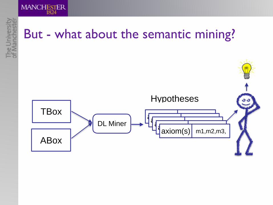
But - what about the semantic mining?
TBox
ABox
DL Miner
Hypotheses
axiom(s) m1,m2,m3,axiom(s) m1,m2,m3,axiom(s) m1,m2,m3,axiom(s) m1,m2,m3,axiom(s) m1,m2,m3,

So, what have we got? (new version)
✓ Loads of measures to capture aspects of hypotheses – mostly independent– some superfluous on positive data (unsurprisingly)
✓Hypothesis generation & evaluation is feasible – provided our ontology is classifiable – provided our search space isn’t too massive
• …focus!
• Which measures indicate interesting hypothesis?• What is the shape for interesting hypothesis?
– are longer/bigger hypotheses better?
• What do we do with them? – how do we guide users through these?

Design, run, analyse survey
Can we learn hypotheses are • usefull/interesting?
…and how does this correlate with measures?
TBox SROIQ sig = 522
ABox 169K CAs 405K RAs
DL Miner
S1: 60 Hypos unfocused S2: 60 Hypos focused
axiom(s) m1,m2,m3,axiom(s) m1,m2,m3,axiom(s) m1,m2,m3,axiom(s) m1,m2,m3,axiom(s) m1,m2,m3,
SHI |Ci| <= 4
30 high-confidence30 low-confidence

Design, run, analyse survey
Can we learn hypotheses are • usefull/interesting?
…and how does this correlate with measures?
TBox SROIQ sig = 522
ABox 169K CAs 405K RAs
DL Miner
S1: 60 Hypos unfocused S2: 60 Hypos focused
axiom(s) m1,m2,m3,axiom(s) m1,m2,m3,axiom(s) m1,m2,m3,axiom(s) m1,m2,m3,axiom(s) m1,m2,m3,
SHI |Ci| <= 4
Valid? Interesting?
30 high-confidence30 low-confidence

Design, run, analyse survey
9.4. CASE STUDIES 221
Validity Interestingness0 1 2 3 4
Wrong 6 11 30 - -Survey 1 Don’t know - 1 - 2 4
(unfocused) Correct - - - 6 -Wrong 1 - 1 - 5
Survey 2 Don’t know - - - - 49(focused) Correct - - - - 4
Table 9.10: Assessment of hypotheses acquired by DL-Miner for ntds: distribu-tion of answers in Survey 1 and Survey 2 (“-” denotes zero)
As Table 9.10 shows, Survey 1 contains 47 hypotheses deemed to be wrong,7 hypotheses unknown, and 6 hypotheses correct. The majority of wrong hypo-theses are of average interestingness (marked by 2) and the rest of wrong hypo-theses are less interesting (marked by 0 or 1). As the domain expert points outin her feedback, wrong hypotheses which are marked by the interestingness of 2indicate data bias, i.e. those are incorrect but strongly supported by the data.According to the results, unknown and correct hypotheses appear to be muchmore interesting than wrong ones: all of them, except one, have high values ofinterestingness (marked by 3 and 4). Amongst those, unknown hypotheses aremarked to be the most interesting and, according to the expert’s response, re-quire further analysis. Overall, 12 out of 60 hypotheses (20%) are found to beinteresting.
The results of Survey 2 are much different from the results of Survey 1, seeTable 9.10. While most hypotheses in Survey 1 are deemed to be wrong, mosthypotheses (49 out of 60) in Survey 2 are marked as unknown. Another noticeabledifference is that all hypotheses, except two, in Survey 2 are marked by the highestvalue of interestingness, i.e. 58 out of 60 hypotheses (⇡ 96.7%), including wrongones, are very interesting in expert’s opinion. Moreover, the expert informedus in her response that one of the wrong hypotheses, besides indicating databias, revealed an error in the ontology. Thus, if focus terms are specified by thedomain expert, the resulting focused hypotheses appear to be significantly moreinteresting than unfocused ones. This is not surprising because, by providingfocus terms, the expert expresses her interest in exploring hypotheses about thoseterms. In addition, the expert is likely to inquire into the domain area which sheknows less about. As a result, the majority of focused hypotheses are deemed to
How good/valid are the mined hypotheses?

Design, run, analyse survey
How does validity/interestingness correlate with our metrics?

Design, run, analyse survey
How does validity/interestingness correlate with our metrics?
9.4. CASE STUDIES 223
−0.7−0.6−0.5−0.4−0.3−0.2−0.1
0.00.10.20.30.40.50.60.7
LENG
THST
REN
DISS
IMBC
ONF
CONF
DEPT
HBC
ONVQ
CONV
QFI
TNBL
IFT
LIFT
BCON
VNCO
NVN
CONT
RBR
AVBA
SSUM
ASSU
MBS
UPP
SUPP
COM
PL
Corre
lation
coef
ficien
t
negative
positive
(a) Survey 1: Validity
−0.7−0.6−0.5−0.4−0.3−0.2−0.1
0.00.10.20.30.40.50.60.7
BCON
FCO
NFLE
NGTH
BCON
VQCO
NVQ
DEPT
HST
REN
BLIF
TLI
FTDI
SSIM
BCON
VNCO
NVN
CONT
RBR
AVFI
TNBS
UPP
SUPP
BASS
UMAS
SUM
COM
PL
Corre
lation
coef
ficien
t
negative
positive
(b) Survey 1: Interestingness
−0.7−0.6−0.5−0.4−0.3−0.2−0.1
0.00.10.20.30.40.50.60.7
BLIF
T
LIFT
LENG
TH
DEPT
H
DISS
IM
BCON
VQ
CONV
Q
BCON
F
CONF
BASS
UM
ASSU
M
FITN
BRAV
BSUP
P
SUPP
COM
PL
Corre
lation
coef
ficien
t
negative
positive
(c) Survey 2: Validity
−0.7−0.6−0.5−0.4−0.3−0.2−0.1
0.00.10.20.30.40.50.60.7
LENG
TH
DEPT
H
DISS
IM
BLIF
T
LIFT
BCON
F
CONF
BCON
VQ
CONV
Q
FITN
BSUP
P
SUPP
BRAV
BASS
UM
ASSU
M
COM
PL
Corre
lation
coef
ficien
t
negative
positive
(d) Survey 2: Interestingness
Figure 9.8: Correlations (in descending order) between hypothesis quality meas-ures and expert’s judgements (4 measures are not shown for Survey 2 becausetheir deviations equal zero and correlation coefficients cannot be calculated)
likely to be “general”, i.e. reflecting known, easily seen patterns of the data.Those hypotheses are not as surprising as “specific” ones which, on the contrary,are likely to reflect uncommon, hardly seen patterns of the data.
The results in Figure 9.8c are similar to the results in Figure 9.8a: the correla-tions for validity look almost equally distributed. The main difference is that liftturns from a non-indicator in Survey 1 to a strong positive indicator in Survey2. One possible reason is that Survey 2 consists of “specific” hypotheses. Suchhypotheses are likely to have a higher lift than “general” hypotheses in Survey 1(since the denominator decreases faster than the numerator, see Definition 5.16).
In comparison to Figure 9.8b for Survey 1, Figure 9.8d for Survey 2 showsconsiderably stronger correlations for interestingness. This may be caused bythe much higher fraction of interesting hypotheses in Survey 2 in comparison to
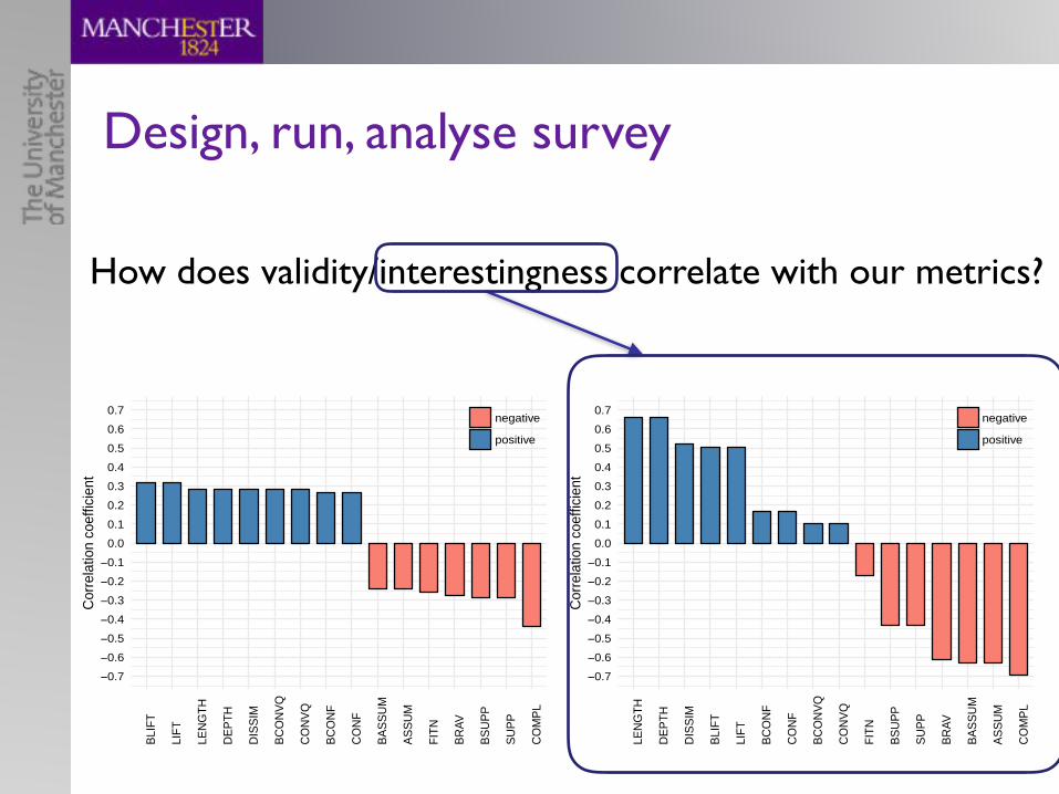

What we learned: 3 kinds of hypotheses!
TBox
ABox
DL Miner
Hypotheses
axiom(s) m1,m2,m3,axiom(s) m1,m2,m3,axiom(s) m1,m2,m3,axiom(s) m1,m2,m3,axiom(s) m1,m2,m3,
high confidence/lift/…low assumptions/braveness
1. An interesting hypothesis can give new insights into domain

Semantic Mining
What we learned: 3 kinds of hypotheses!
TBox
ABox
DL Miner
Hypotheses
axiom(s) m1,m2,m3,axiom(s) m1,m2,m3,axiom(s) m1,m2,m3,axiom(s) m1,m2,m3,axiom(s) m1,m2,m3,
high confidence/lift/…low assumptions/braveness
1. An interesting hypothesis can give new insights into domain
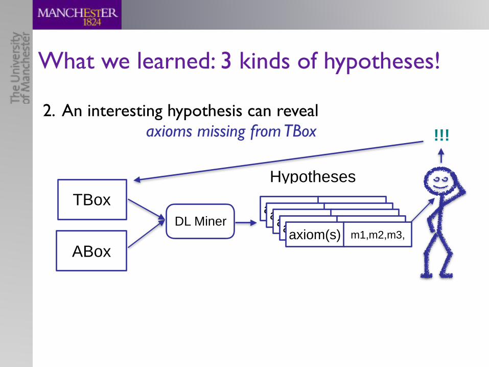
What we learned: 3 kinds of hypotheses!
TBox
ABox
DL Miner
Hypotheses
axiom(s) m1,m2,m3,axiom(s) m1,m2,m3,axiom(s) m1,m2,m3,axiom(s) m1,m2,m3,axiom(s) m1,m2,m3,
2. An interesting hypothesis can reveal axioms missing from TBox !!!

What we learned: 3 kinds of hypotheses!
TBox
ABox
DL Miner
Hypotheses
axiom(s) m1,m2,m3,axiom(s) m1,m2,m3,axiom(s) m1,m2,m3,axiom(s) m1,m2,m3,axiom(s) m1,m2,m3,
2. An interesting hypothesis can reveal axioms missing from TBox
TBox completionontology learning from data
!!!

What we learned: 3 kinds of hypotheses!
3. An interesting hypothesis can reveal bias & errors in the ontology
high confidence/lift/…low assumptions/braveness
TBox
ABox
DL Miner
Hypotheses
axiom(s) m1,m2,m3,axiom(s) m1,m2,m3,axiom(s) m1,m2,m3,axiom(s) m1,m2,m3,axiom(s) m1,m2,m3,

What we learned: 3 kinds of hypotheses!
3. An interesting hypothesis can reveal bias & errors in the ontology
high confidence/lift/…low assumptions/braveness
TBox
ABox
DL Miner
Hypotheses
axiom(s) m1,m2,m3,axiom(s) m1,m2,m3,axiom(s) m1,m2,m3,axiom(s) m1,m2,m3,axiom(s) m1,m2,m3,
???
Semantic Data Analysis

3 kinds of hypotheses - can we predict?
TBox
ABox
DL Miner
Hypotheses
axiom(s) m1,m2,m3,axiom(s) m1,m2,m3,axiom(s) m1,m2,m3,axiom(s) m1,m2,m3,axiom(s) m1,m2,m3,
high confidence/lift/… low assumptions/braveness
No - they look alike

3 kinds of hypotheses - can we predict?
TBox
ABox
DL Miner
Hypotheses
axiom(s) m1,m2,m3,axiom(s) m1,m2,m3,axiom(s) m1,m2,m3,axiom(s) m1,m2,m3,axiom(s) m1,m2,m3,
high confidence/lift/… low assumptions/braveness
No - they look alikePerhaps - with different ABoxes/other sources

Summary & Outlook• Mining rich axioms from ontologies is possible
– gives us more than we thought – expressive axioms are better!
• Fine test case for incremental/ABox reasoning
• More surveys– to better understand relevance of metrics– but we’ve got the shape now
• Redundancy in general is tricky & costly– stripping superfluous parts from concepts, (sets of) axioms
• We need even better refinement operators: – for more expressive DLs– redundancy-free– ontology-aware
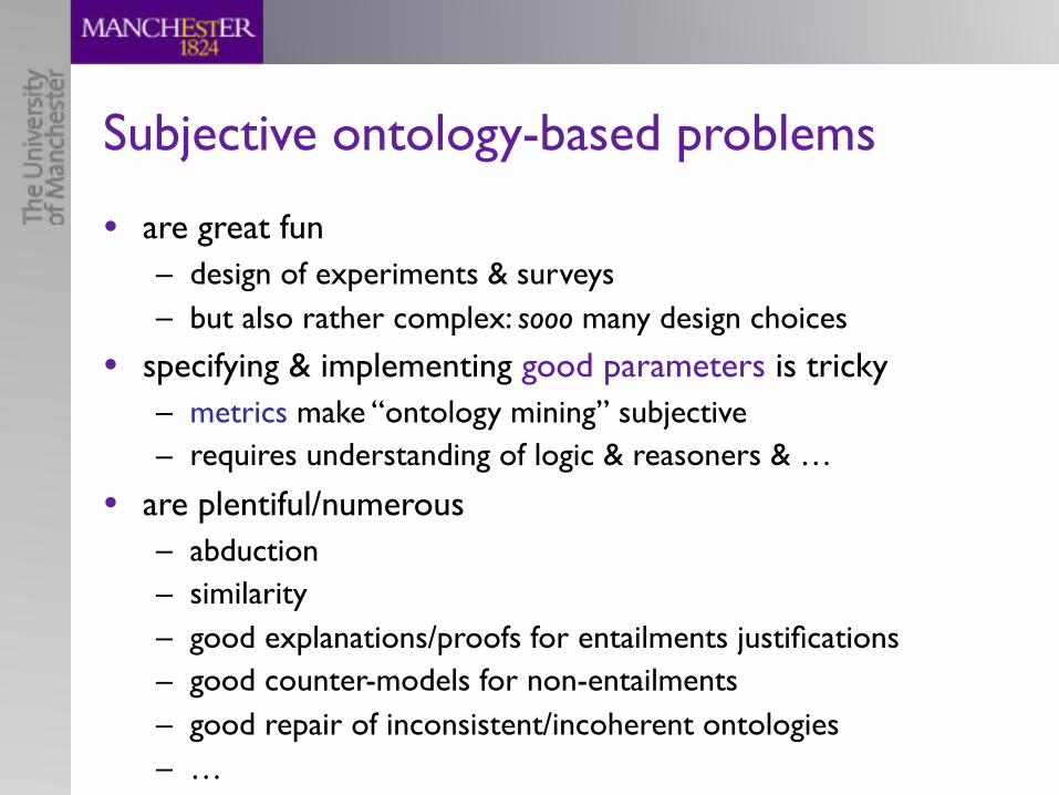
Subjective ontology-based problems
• are great fun– design of experiments & surveys– but also rather complex: sooo many design choices
• specifying & implementing good parameters is tricky– metrics make “ontology mining” subjective– requires understanding of logic & reasoners & …
• are plentiful/numerous– abduction– similarity – good explanations/proofs for entailments justifications– good counter-models for non-entailments– good repair of inconsistent/incoherent ontologies– …

Special Thanks to
Slava Sazonau

Some Advertisement
Cover illustration: The Description Logic logo. Courtesy of Enrico Franconi.
Baader, Horrocks,
Lutz, SattlerAn Introduction to D
escription Logic
Description Logics (DLs) have a long tradition in computer science and knowledge representation, being designed so that domain knowledge can be described and so that computers can reason about this knowledge. DLs have recently gained increased importance since they form the logical basis of widely used ontology languages, in particular the web ontology language OWL.
Written by four renowned experts, this is the first textbook on Description Logic. It is suitable for self-study by graduates and as the basis for a university course. Starting from a basic DL, the book introduces the reader to their syntax, semantics, reasoning problems and model theory, and discusses the computational complexity of these reasoning problems and algorithms to solve them. It then explores a variety of reasoning techniques, knowledge-based applications and tools, and describes the relationship between DLs and OWL.
Franz Baader is a professor in the Institute of Theoretical Computer Science at TU Dresden.
Ian Horrocks is a professor in the Department of Computer Science at the University of Oxford.
Carsten Lutz is a professor in the Department of Computer Science at the University of Bremen.
Uli Sattler is a professor in the Information Management Group within the School of Computer Science at the University of Manchester.
Designed by Zoe Naylor.
9780521873611 Baader et al. PPC C M Y
K Description LogicAn Introduction to
Franz BaaderIan Horrocks Carsten Lutz Uli Sattler
Get 20% Discount: For more information, and to order, visit:
www.cambridge.org/9780521695428 and enter the code BAADER2017 at the checkout
An Introduction toDescription Logic
Description logics (DLs) have a long tradition in computer science andknowledge representation, being designed so that domain knowledge canbe described and so that computers can reason about this knowledge. DLshave recently gained increased importance since they form the logical basisof widely used ontology languages, in particular the web ontology languageOWL. Written by four renowned experts, this is the first textbook ondescription logics. It is suitable for self-study by graduates and as the basisfor a university course. Starting from a basic DL, the book introduces thereader to their syntax, semantics, reasoning problems and model theoryand discusses the computational complexity of these reasoning problemsand algorithms to solve them. It then explores a variety of reasoningtechniques, knowledge-based applications and tools and it describes therelationship between DLs and OWL.
on this titleExpires 15 March 2018
Technische Universität, DresdenFranz Baader
University of OxfordIan Horrocks
Universität BremenCarsten Lutz
University of Manchesterand Uli Sattler
1. Introduction; 2. A basic DL; 3. A little bit of model theory; 4. Reasoning in DLs with tableaualgorithms; 5. Complexity; 6. Reasoning in the εL family of Description Logics; 7. Queryanswering; 8. Ontology languages and applications; Appendix A. Description Logicterminology; References; Index.
20% Discount
£59.99 £47.99Discount priceOriginal price
$79.99 $63.99
£29.99 £23.99Discount priceOriginal price
$39.99 $31.99
Hardback 978-0-521-87361-1
Paperback 978-0-521-69542-8
April 2017228 x 152 mm 260pp 30 b/w illus.