UMEA UNIVERSITY DOCTORAL DISSERTATIONS

ISBN 978-91-7459-016-6

From Protein Sequence to Structural

Instability and Disease

Lixiao Wang

Department of Chemistry

Umeå University, Sweden

Umeå 2010

Copyright © 2010 Lixiao Wang

ISBN: 978-91-7459-016-6

Printed by: Print & Media

Umeå, Sweden 2010

To my family

学而不思则罔，思而不学则殆 Learning without thinking leads to confusion

thinking without learning ends in danger

孔子 Confucius

I

Abstract

A great challenge in bioinformatics is to accurately predict protein structure and

function from its amino acid sequence, including annotation of protein domains,

identification of protein disordered regions and detecting protein stability changes

resulting from amino acid mutations. The combination of bioinformatics, genomics

and proteomics becomes essential for the investigation of biological, cellular and

molecular aspects of disease, and therefore can greatly contribute to the

understanding of protein structures and facilitating drug discovery.

In this thesis, a PREDICTOR, which consists of three machine learning methods

applied to three different but related structure bioinformatics tasks, is presented:

using profile Hidden Markov Models (HMMs) to identify remote sequence

homologues, on the basis of protein domains; predicting order and disorder in

proteins using Conditional Random Fields (CRFs); applying Support Vector

Machines (SVMs) to detect protein stability changes due to single mutation.

To facilitate structural instability and disease studies, these methods are

implemented in three web servers: FISH, OnD-CRF and ProSMS, respectively.

For FISH, most of the work presented in the thesis focuses on the design and

construction of the web-server. The server is based on a collection of structure-

anchored hidden Markov models (saHMM), which are used to identify structural

similarity on the protein domain level.

For the order and disorder prediction server, OnD-CRF, I implemented two

schemes to alleviate the imbalance problem between ordered and disordered amino

acids in the training dataset. One uses pruning of the protein sequence in order to

obtain a balanced training dataset. The other tries to find the optimal p-value cut-off

for discriminating between ordered and disordered amino acids. Both these

schemes enhance the sensitivity of detecting disordered amino acids in proteins. In

addition, the output from the OnD-CRF web server can also be used to identify

flexible regions, as well as predicting the effect of mutations on protein stability.

For ProSMS, we propose, after careful evaluation with different methods, a

clustered by homology and a non-clustered model for a three-state classification of

protein stability changes due to single amino acid mutations. Results for the non-

clustered model reveal that the sequence-only based prediction accuracy is

comparable to the accuracy based on protein 3D structure information. In the case

of the clustered model, however, the prediction accuracy is significantly improved

when protein tertiary structure information, in form of local environmental

conditions, is included. Comparing the prediction accuracies for the two models

indicates that the prediction of mutation stability of proteins that are not

homologous is still a challenging task.

Benchmarking results show that, as stand-alone programs, these predictors can be

comparable or superior to previously established predictors. Combined into a

program package, these mutually complementary predictors will facilitate the

understanding of structural instability and disease from protein sequence.

II

III

List of publications

I. Tångrot J., Wang L., Kågström B. and Sauer UH. (2006) FISH –

Family Identification of Sequence Homologues using Structure

Anchored Hidden Markov Models. Nucleic Acid Research v.34 (Web

server issue), W10-W14.

II. Tångrot J., Wang L., Kågström B. and Sauer UH. (2007) Design,

construction and use of the FISH server. In Applied Parallel Computing:

State of the Art in Scientific Computing, PARA 2006, Lecture Notes in

Computer Science, LNCS4699, Springer-Verlag, pp 647-657.

III. Wang L. and Sauer UH. (2008) OnD-CRF: predicting order and

disorder in proteins using conditional random fields. Bioinformatics,

24(11), 1401-1402.

IV. Wang L. and Sauer UH. (2010) Prediction of protein stability changes

due to single amino acid mutations. (manuscript)

IV

Abbreviations

3D Three-Dimensional

NMR Nuclear Magnetic Resonance

IDPs Intrinsically Disordered Proteins

IUPs Intrinsically Unstructured Proteins

MoRFs Molecular Recognition Features

MoREs Molecular Recognition Elements

PDB Protein Data Bank

DSSP Definition of the secondary structure of protein

HCA Hydrophobic Cluster Analysis

CASP Critical Assessment of techniques for protein

Structure Prediction

SCOP Structural Classification of Proteins

CRFs Conditional Random Fields

HMMs Hidden Markov Models

DRs Disordered Regions

ROC Receiver Operating Characteristic

AUC Area Under the Curve

SVMs Support Vector Machines

OVA One-Versus-All

OVO One-Versus-One

V

Contents

1. Introduction ................................................................................................. 1

1.1 Biological background ......................................................................... 1

1.1.1 Protein structure ........................................................................... 1

1.1.2 Intrinsically disordered protein .................................................... 4

1.1.3 Protein stability ............................................................................ 8

1.2 Machine learning in Bioinformatics .................................................. 11

1.2.1 Prediction of protein disorder .................................................... 14

1.2.2 Prediction for protein stability change due to point mutation ... 15

1.3 Research goal and scope .................................................................... 16

2. Material and methods ................................................................................ 18

2.1 Construction of FISH server .............................................................. 18

2.1.1 Structure anchored Hidden Markov Models (saHMM) ............. 18

2.1.2 Architecture of the FISH server ................................................. 19

2.2 Predicting protein order and disorder ................................................ 20

2.2.1 Dataset ....................................................................................... 20

2.2.2 Conditional random fields (CRFs)............................................. 22

2.2.3 Feature selection ........................................................................ 24

2.2.4 Model building .......................................................................... 25

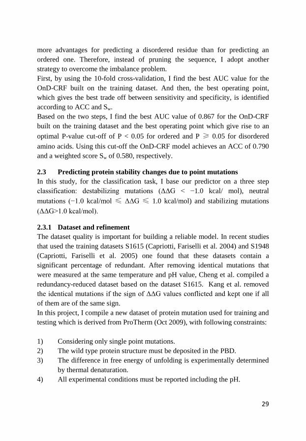
2.3 Predicting protein stability changes due to point mutations .............. 29

2.3.1 Dataset and refinement .............................................................. 29

2.3.2 Support vector machines (SVMs) .............................................. 34

2.3.3 Feature selection ........................................................................ 36

2.3.4 Non-clustered model .................................................................. 39

2.3.5 Clustered model for 3-state classification .................................. 41

3. Evaluation criteria ..................................................................................... 43

VI

3.1 Cross validation ................................................................................. 43

3.1.1 Procedures of cross-validation ................................................... 43

3.1.2 Key Application ......................................................................... 43

3.2 Assessment of classification .............................................................. 44

3.2.1 Sensitivity and specificity .......................................................... 44

3.2.2 ROC curve ................................................................................. 45

3.2.3 S-product, Sw and ACC ............................................................ 45

3.2.4 Matthews‟ correlation coefficient .............................................. 46

3.3 Assessment of Regression ................................................................. 46

3.3.1 Pearson's correlation .................................................................. 46

3.3.2 Mean absolute error (MAE) and the standard error of estimate 46

4. Contributions and relate works .................................................................. 47

4.1 Construction of FISH server (Paper I, II) .......................................... 47

4.2 Prediction of order and disorder in proteins (Paper III)..................... 48

4.3 Prediction of protein mutation-induced stability change (Paper IV) . 55

5. Conclusions ............................................................................................... 57

6. Future plan ................................................................................................. 58

7. Acknowledgement ..................................................................................... 59

8. References ................................................................................................. 61

1

1. Introduction Bioinformatics is the cross-disciplinary field that uses computational methods to

solve problems in the life sciences. The most impressive task in this field is to

develop tools and resources that aid in the analysis and interpretation of various

types of data. Development of these tools or resources requires extensive

computing knowledge, as well as a thorough understanding of biology.

1.1 Biological background

1.1.1 Protein structure

Proteins are linear polypeptides composed of 20 different naturally occurring

amino acids whose structures are shown in Figure 1. The chemical structure of

each amino acid contains a hydrogen atom (H), an amino group (NH2) and an

acid group (COOH) in common which are attached to the alpha carbon (Cα).

The side chain attached to the fourth valence of the Cα atom leads to the

different properties of each amino acid and has a major influence on how

proteins fold and stabilized. The 20 amino acids can be divided into different

classes, according to the physico-chemical properties of their side chains

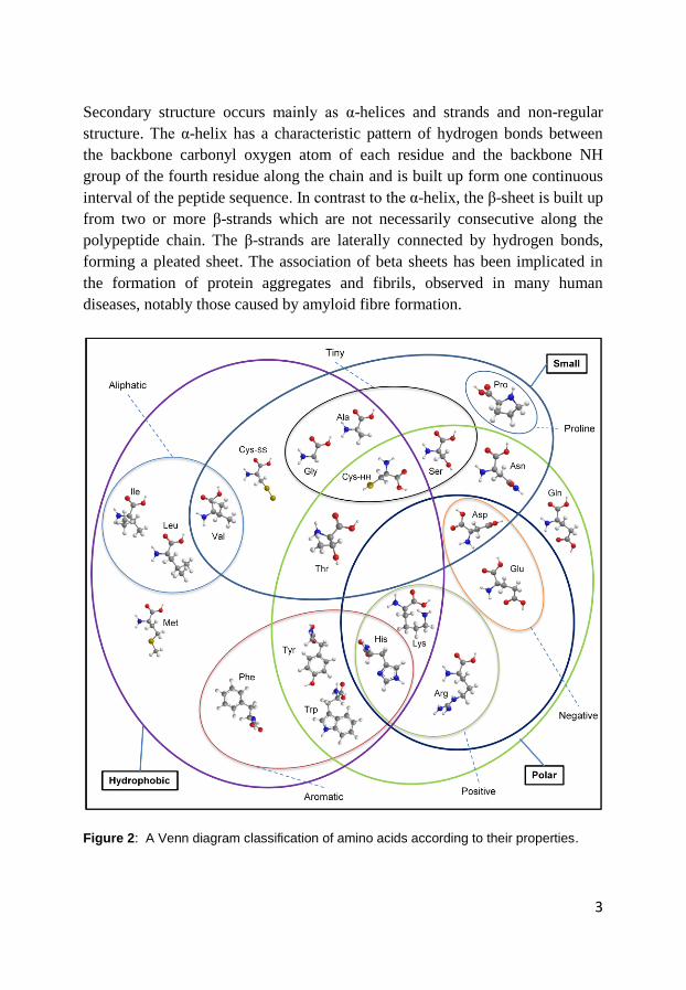
(Taylor 1986; Livingstone and Barton 1993) as shown in Figure 2. The key

features are the charge, the overall size and the hydrophobicity of the side chain.

During peptide synthesis, the ribosome connects the amino acids through

peptide bonds as the chain is extended. In general, the protein chain starts from

the N-terminal end, which contains a free amino group to the C-terminal end

that contains a free carboxyl group. The formation of a series of peptide bonds

generates a “backbone” or “main chain” from which the various side chains

project. The succession of the side chain atoms in order away from the

backbone are usually designated as β, γ, δ, ε, δ and ε.

Proteins are generally described in terms of “primary”, “secondary”, “tertiary”

and “quaternary” structure to emphasize the structural hierarchy in proteins.

The sequence of amino acids in a polypeptide chain is known as the primary

structure. Many natural protein sequences are found to be similar to varying

extents; some are virtually identical, while others show barely significant

resemblance. Any statistically significant sequence similarity is taken as an

indication that the two proteins might have a common evolutionary ancestor, in

which case they are said to be homologous. The sequence similarities between

2

homologous proteins are very powerful tools in reconstructing the process of

evolution (Wilson, Carlson et al. 1977; Felsenstein 1988). Sequence identity

and similarity are very powerful means for identifying the function of a newly

sequenced protein, so considerable effort has been invested to develop more

rapid and more powerful sequence comparison methods.

Figure 1: The chemical structure of the 20 amino acids of proteins. Only side chains are

shown, except for the first amino acid, alanine, where all atoms are shown. The bond

from the side chain to Cα is red. The full name, the three-letter and one-ltter codes are

given for each amino acid.

3

Secondary structure occurs mainly as α-helices and strands and non-regular

structure. The α-helix has a characteristic pattern of hydrogen bonds between

the backbone carbonyl oxygen atom of each residue and the backbone NH

group of the fourth residue along the chain and is built up form one continuous

interval of the peptide sequence. In contrast to the α-helix, the β-sheet is built up

from two or more β-strands which are not necessarily consecutive along the

polypeptide chain. The β-strands are laterally connected by hydrogen bonds,

forming a pleated sheet. The association of beta sheets has been implicated in

the formation of protein aggregates and fibrils, observed in many human

diseases, notably those caused by amyloid fibre formation.

Figure 2: A Venn diagram classification of amino acids according to their properties.

4

Secondary structure elements usually arrange themselves in motifs which are

formed by certain packing of secondary structure elements. Several motifs in a

protein usually combine to form compact globular structures, which are called

domains. Domains can exhibit catalytic, regulatory and recognition functions

and their combinatorial varieties supply an almost inexhaustible repertoire of

building blocks for complex signalling/regulatory systems. Domains can be

grouped into families by sequence similarities that suggest a common

evolutionary origin. Establishing such relationships has become an important

first line of analysis in any attempt to uncover the function of a novel protein, or

even to characterize an entire genome. Data bases such as the Structural

Classification of Proteins, SCOP, data base (Andreeva, Howorth et al. 2004)

contain a hierarchical clustering of domains on the class, fold, super family and

family level.

Tertiary structure describes both for the way motifs are arranged into domain

structures and for the way a single polypeptide chain folds into one or several

domains.

A fairly large number of proteins assemble into a quaternary structure, which

consists of several identical or non-identical polypeptide chains that associate

into a multimeric molecule.

The traditional view of structural biology: “one sequence, one structure, one

function” assumes that proteins are biologically active only when folded in their

native conformation. Therefore, understanding their three-dimensional structure

is the key to understanding how they function. Most protein structures are

determined by X-ray crystallography and NMR spectroscopy. X-ray crystal

structures are usually more detailed and contain some information about

flexibility, whereas NMR techniques provide additional dynamic information

concerning flexibility and motion within the protein structure.

1.1.2 Intrinsically disordered protein

In contrast to the traditional view, significant experimental and computational

data have recently confirmed that many proteins or parts of proteins lack a

specific 3D structure in their native state. Nevertheless, these proteins are able

to carry out essential biological functions in key biological processes (Wright

and Dyson 1999; Uversky, Gillespie et al. 2000; Dunker, Lawson et al. 2001;

Tompa 2002). These proteins and protein segments are collectively called

intrinsically disordered proteins, IDPs, or intrinsically unstructured proteins,

IUPs.

5

In a survey, Dunker et al. have identified at least twenty-eight different

functions that are associated with IDPs and ID/IU regions (Dunker, Brown et al.

2002). The most common function involves protein-protein interactions,

followed by protein–DNA and protein–RNA binding. Furthermore, Dunker et al.

proposed four major functional classes: molecular recognition, molecular

assembly and/or disassembly, protein post-translational modification and

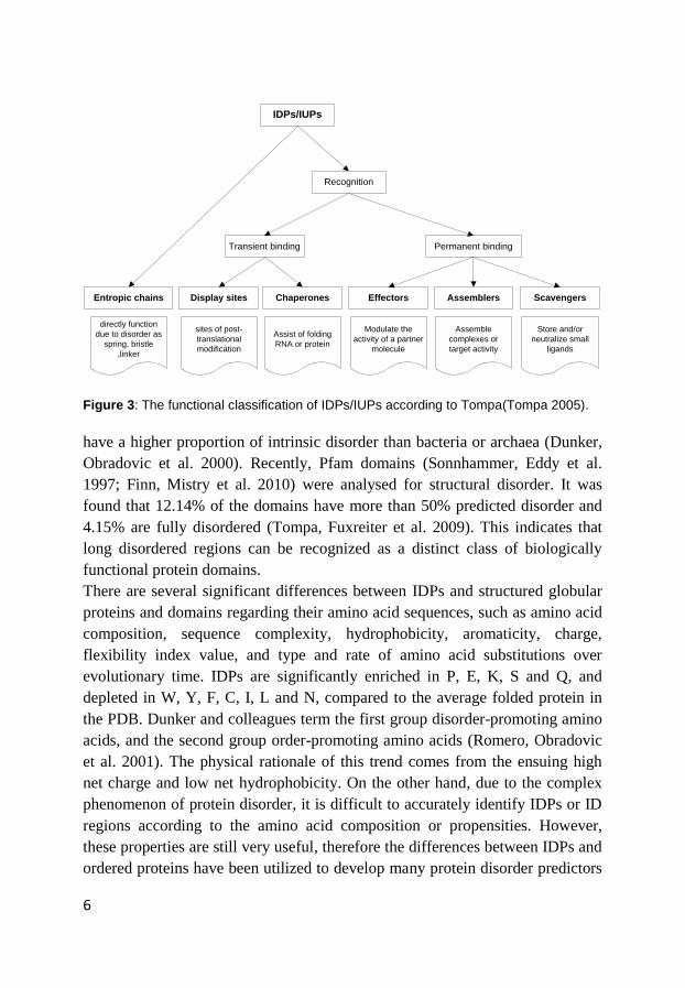
entropic chains (Dunker, Brown et al. 2002). Similarly, as shown in Figure 3,

Tompa classified these 28 functions into five distinct functional classes (Tompa

2005). Many experimental results show that disordered regions can undergo a

disorder-to-order transition upon binding to a structured complement which is

not the case for entropic chains whose functions directly stem from the

disordered state (Tompa 2005). Disorder-to-order transitions play a crucial role

in macromolecular recognition. There are numerous examples of protein-protein,

protein-nucleic acid, and protein-ligand interactions involving disordered

protein segments. A specialized subset of these interacting domains have been

recognized as „Molecular Recognition Features, MoRFs, or Molecular

Recognition Elements, MoREs‟ (Uversky, Oldfield et al. 2005) which are

protein regions that specifically participate in protein-protein interactions. These

various functions of IDPs and ID regions complement the functional repertoire

of ordered regions (Xie, Vucetic et al. 2007), which have evolved mainly to

carry out efficient catalysis (Radivojac, Iakoucheva et al. 2007).

By using bioinformatics methods, the prediction results indicate that sequence

databases such as SWISS-PROT and PIR contain proteins with significantly

higher fractions of predictions of long regions of disorder as compared to the

sequences in the PDB(Romero, Obradovic et al. 1998; Dunker, Obradovic et al.

2000; Romero, Obradovic et al. 2001). These data suggested that nature

produced proteins which are quite rich in disorder and furthermore that the PDB

is strongly biased against intrinsic disorder, probably because of the

requirement for crystallization (Romero, Obradovic et al. 1998). Further

analysis of predicted protein disorder indicates that eukaryotic proteins

6

IDPs/IUPs

Entropic chains

Recognition

Transient binding Permanent binding

Display sites Chaperones Effectors Assemblers Scavengers

directly function

due to disorder as

spring, bristle

,linker

sites of post-

translational

modification

Assist of folding

RNA or protein

Modulate the

activity of a partner

molecule

Assemble

complexes or

target activity

Store and/or

neutralize small

ligands

Figure 3: The functional classification of IDPs/IUPs according to Tompa(Tompa 2005).

have a higher proportion of intrinsic disorder than bacteria or archaea (Dunker,

Obradovic et al. 2000). Recently, Pfam domains (Sonnhammer, Eddy et al.

1997; Finn, Mistry et al. 2010) were analysed for structural disorder. It was

found that 12.14% of the domains have more than 50% predicted disorder and

4.15% are fully disordered (Tompa, Fuxreiter et al. 2009). This indicates that

long disordered regions can be recognized as a distinct class of biologically

functional protein domains.

There are several significant differences between IDPs and structured globular

proteins and domains regarding their amino acid sequences, such as amino acid

composition, sequence complexity, hydrophobicity, aromaticity, charge,

flexibility index value, and type and rate of amino acid substitutions over

evolutionary time. IDPs are significantly enriched in P, E, K, S and Q, and

depleted in W, Y, F, C, I, L and N, compared to the average folded protein in

the PDB. Dunker and colleagues term the first group disorder-promoting amino

acids, and the second group order-promoting amino acids (Romero, Obradovic

et al. 2001). The physical rationale of this trend comes from the ensuing high

net charge and low net hydrophobicity. On the other hand, due to the complex

phenomenon of protein disorder, it is difficult to accurately identify IDPs or ID

regions according to the amino acid composition or propensities. However,

these properties are still very useful, therefore the differences between IDPs and

ordered proteins have been utilized to develop many protein disorder predictors

7

for predicting disordered regions from amino acid sequences (Romero,

Obradovic et al. 2001).

Low-sequence complexity is another useful property to identify disordered

regions in amino acid sequences. Wotten, who introduced the term low

complexity for protein sequences (Wootton 1994), observed that low

complexity regions in proteins deviate significantly from the amino acid

composition typically observed for globular proteins. The reason is the

repetitive nature of their sequences and/or because few amino acids dominate

the distribution. It was shown that low-sequence complexity segments often

appear in disordered proteins (Romero, Obradovic et al. 2001). Nevertheless, it

is not a general rule. Low-complexity sequences can also form ordered structure

under some circumstances, such as coiled-coils or other fibrous proteins. So,

low-sequence complexity is limited to one single aspect of protein disorder.

Alone, it is not sufficient to accurately identify IDPs or ID regions. However, it

provides useful information for further protein sequence analysis.

Different lengths of protein disordered regions also have significant differences

in their amino acid compositions (Romero P 1997; Radivojac, Obradovic et al.

2004; Obradovic, Peng et al. 2005). The general agreement is that the length

threshold for a short disordered region is 30 amino acids.

Many IDPs are associated with a wide array of diseases, such as cancer

(Iakoucheva, Brown et al. 2002), diabetes, autoimmune diseases, cardiovascular

disease (Cheng, LeGall et al. 2006), amyloidoses, neurodegenerative diseases

(Chiti and Dobson 2006), and others. This indicates that structural disorder

poses a particular danger to the organism. Therefore, identifying and

understanding the mechanistic details of their functioning particularly with

respect to interaction with their binding partners can contribute new potential

target for future drug discovery.

8

1.1.3 Protein stability

Understanding the amino-acid sequence determinants of protein stability and

function is important for protein structure-function study. Genetic studies of

protein structure and activity generally centre on the properties of proteins

altered by deletions or point mutations (Pakula and Sauer 1989).

A wide range of experimental techniques can be used to measure the

conformational stability of a protein, often determined as the difference in

stability between the wild type protein and a variant, differing by a single amino

acid mutation. These techniques rely on specific spectroscopic methods

(Dobson and Karplus 1999), such as circular dichroism and fluorescence, and

use specific ways to initiate protein (un)folding processes. Most frequently one

uses thermal and chemical denaturation in the case of proteins.

In the simplest case, globular proteins fold and unfold spontaneously in a

reaction that can be described in terms of a simple, two-state equilibrium as

N D (1) Such two-state behaviour leads directly to an expression for the equilibrium

constant, Kd, which is a measure of the ratio of unfolded to folded protein

molecules.

dK D / N (2)

where [N] and [D] represent the concentrations of the native and denatured

states, respectively.

The difference between the Gibbs free energies of the folded and the unfolded

states, ΔG, can be calculated from Kd by:

dG RTln K (3)

where R is the gas constant, T is the absolute temperature.

The conformational changes during unfolding can be monitored by changes in

the circular dichroism (CD), UV, or fluorescence signal as a function of the

denaturant concentration (Pace 1986). For thermal denaturation monitored by

calorimetry methods, the changes in the conformational stability of the protein

are monitored by the global heat exchange between the protein and solvent as a

function of temperature (Privalov and Khechinashvili 1974).

9

Figure 4: A simplified diagram illustrates that during the folding process the protein

proceeds from a high energy unfold state to a low energy native state. The Gibbs free

energy difference between the mutant and wild-type protein is the free energy change,

ΔΔG.

The free energy change between a mutated protein and the WT protein can be

defined as

mu wtG G G (4)

If the energy change ΔΔG is positive, the mutation has increased stability. If

ΔΔG is negative, the mutation is destabilizing the protein.

Non-covalent interactions between different atoms of a protein are especially

important in defining and stabilizing the three-dimensional structure of the

protein, in which atoms distant in the covalent structure can interact at close

range. These interactions are generally considered to be of four types:

electrostatic interaction between charges and dipoles, van der Waals forces,

hydrogen bonds, and hydrophobic interactions. Owing to protein structures

containing a large number of these stabilizing interactions, it is often difficult to

imagine that a point mutation could result in a serious perturbation of structure

or stability. Experimental results show that most naturally accepted mutations

10

have negligible effect on the fitness of the organism (Shortle and Lin 1985;

Pakula, Young et al. 1986; Loeb, Swanstrom et al. 1989; Guo, Choe et al. 2004).

This forms the basis of the so called neutral theory of evolution (King and Jukes

1969; Kimura 1983), which states that many mutations do not affect the protein

much, they tend to conserve the proteins native fold and its biochemical (Bloom,

Silberg et al. 2005; Bhattacherjee and Biswas 2009).

On the other hand, as the protein goes from a denatured state with many

possible conformations to a native state with only one or a few conformations,

almost all of its freedom is lost. Generally, the ΔGfold is small, often less than

10kcal/mol under physiological condition. Thus, the native state is only

marginally stable (Savage, Elliott et al. 1993; Ruvinov, Wang et al. 1997; Vogl,

Jatzke et al. 1997; Taverna and Goldstein 2002). Similar to the introduction of

mutations, changes in pH or temperature can turn biologically active proteins in

their native state to a biologically inactive denatured state.

In protein engineering, different approaches have been used to identify

mutations that enhance protein stability, such as rational design, directed

evolution and consensus methods.

By using rational or structure-based design (Eijsink, Bjork et al. 2004), biologist

makes particular amino acid mutations to specifically improve qualities in the

protein‟s structure. These mutations can be made to improve Van der Waals‟

interactions, hydrogen bonds, salt bridges, interactions with ions, and disulfide

bridges as well as several other terms. Since site-directed mutagenesis

techniques are well-developed, this approach is inexpensive and relatively easy.

However, there is a major drawback in that the detailed structural knowledge of

a protein is often unavailable, and even when it is available, it can be extremely

difficult to predict the effects of various mutations.

Directed evolution approaches (Hida, Hanes et al. 2007) apply random

mutagenesis to the initial protein sequence, and these mutations are evaluated

for improvements of specific qualities. The mutants that perform the best are

then used for additional rounds of mutations until the researcher is satisfied with

the results. This method mimics natural evolution and requires no prior

structural knowledge of a protein. The drawback is that it requires a significant

amount of laboratory resources for performing the multiple rounds of mutations

and selections. Therefore, this approach can be both expensive and time-

consuming.

In contrast to rational design, the consensus method does not require knowledge

of the three dimensional structure of the protein and neither does it need the

11

laboratory resources required for directed evolution (Lehmann and Wyss 2001).

It tries to find shared feature or attribute between proteins within the same

family from sequence databases. Usually, the multiple sequence alignment is

first performed together the query sequence with a large number of homologous

sequences. If a majority of the homologous sequences all have the same amino

acid in a particular position and if it is different from the amino acid in the

query sequence, the consensus method states that the amino acid in the query

sequence should be mutated to the amino acid shared by the majority of the

homologous sequences. The drawback is that it requires a large number of

sequences homologous to the target protein, as well as arbitrary constraints for

picking which amino acids to mutate when there is not a clear „majority‟ amino

acid at a given position in the sequence alignment.

1.2 Machine learning in Bioinformatics

Machine learning is a subfield in computational intelligence and is concerned

with the development of algorithms and techniques that allow computers to

learn. Its key idea is to direct the computer to learn how to solve a problem

rather than explicitly give the solution to the computer.

With the exponential growth of the size of the biological databanks, analyzing

and understanding these data have become critical. Traditionally, researchers do

biological research by using their knowledge and intelligence, performing

experiments by hands and eyes, and processing data by basic statistical and

mathematical tools. Due to the huge amounts of biological data and a very large

number of possible combinations and permutations of various biological

sequences, the conventional human intelligence-based methods cannot work

effectively and efficiently. Therefore, many machine learning methods have

been developed to recognize complex patterns and make intelligent decisions

based on data. Hence, machine learning in bioinformatics has become an

important role in complex biological applications.

As shown in Figure 5, machine learning techniques have been widely applied

for knowledge extraction in six different biological domains: genomics,

proteomics, microarray, systems biology, evolution and text mining (Larranaga,

Calvo et al. 2006).

12

Figure 5: Classification of the application where machine learning methods are applied

in bioinformatics (Larranaga, Calvo et al. 2006).

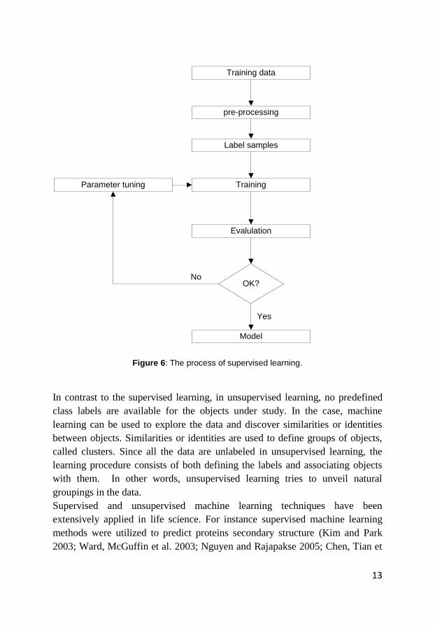
There are two main paradigms in the field of machine learning: supervised and

unsupervised learning. Both have been widely applied in biology.

Supervised learning can be formalized as the problem of inferring a function

y f x based on a training dataset 1 1 n nT x , y , ..., x , y . Usually, the

inputs, or features, are m-dimensional vectors i i, 1 i,mx x ..x . When y is

continuous, we are in the context of regression, whereas in classification

problems, y is of categorical nature. The goal in supervised learning is to

design a system able to accurately predict the class membership or continuous

values of new objects based on the available features. An overview of the

process of supervised learning is shown in Figure 6.

13

Training data

pre-processing

Label samples

Training

Evalulation

Parameter tuning

OK?

Model

No

Yes

Figure 6: The process of supervised learning.

In contrast to the supervised learning, in unsupervised learning, no predefined

class labels are available for the objects under study. In the case, machine

learning can be used to explore the data and discover similarities or identities

between objects. Similarities or identities are used to define groups of objects,

called clusters. Since all the data are unlabeled in unsupervised learning, the

learning procedure consists of both defining the labels and associating objects

with them. In other words, unsupervised learning tries to unveil natural

groupings in the data.

Supervised and unsupervised machine learning techniques have been

extensively applied in life science. For instance supervised machine learning

methods were utilized to predict proteins secondary structure (Kim and Park

2003; Ward, McGuffin et al. 2003; Nguyen and Rajapakse 2005; Chen, Tian et

14

al. 2007; Zhao and Wang 2008) and zinc-binding sites (Shu, Zhou et al. 2008)

from their amino acid sequences.

Unsupervised learning technique, such as hierarchical and k-means clustering,

gene expression data was successfully used to classify patients in different

groups and to identify new disease groups (Aach, Rindone et al. 2000; Zhu and

Zhang 2000).

1.2.1 Prediction of protein disorder

In structural biology, disorder prediction is crucial for protein sequence analysis.

For example, protein disordered regions at the N or C termini or within proteins

often make it difficult to express, purify and crystallize a protein or to measure

its NMR spectrum. Consequently, it can be essential to utilize bioinformatics

tools to predict protein disorder and unstructured regions in order to identify

potentially structured domains. This will facilitate the design of constructs for

3D structure determination and for 3D structure prediction.

Machine learning methods have been successfully applied to predict protein

disorder. There are two mainly used machine learning approaches in the protein

disorder prediction: Neural networks and Support vector machines.

The first disorder prediction method, PONDRVL-XT (Romero, Obradovic et al.

2001), was developed by using feed-forward neural networks based on local

amino acid composition, flexibility and other sequence features. Since then, an

increasing number of machine learning implementations have been developed.

The DisEMBL method(Linding, Jensen et al. 2003) is trained based on artificial

neural networks for predicting different aspect of protein disorder, such as loops

and coils defined by DSSP, loops with high B-factor and missing coordinates in

X-ray structure. PONDR VL3 (Radivojac, Obradovic et al. 2003) is also based

on a neural network but trained on a larger dataset of variously characterised

disorder region than PONDR VL-XT. DISOPRED2 (Ward, Sodhi et al. 2004)

utilizes support vector machine, SVM, for protein disorder prediction. It

incorporates information from multiple sequence alignments that was generated

for each protein using PSI-BLAST. DisPSSMP (Su, Chen et al. 2006) also

incorporates inputs from PSI-BLAST, but uses radial basis function networks as

a training algorithm. RONN (Yang, Thomson et al. 2005) uses a modified

version of radial basis function networks called bio-basis function neural

networks which incorporates information based on similarity to known

disordered segments. DISpro (CHENG, SWEREDOSKI et al. 2005) uses

recurrent networks which incorporate evolutionary information in the form of

15

profiles, predicted secondary structure and relative solvent accessibility, and

ensembles of 1D-recursive neural networks. POODLE-S and POODLE-L

extract features from phsyico-chemical properties using PSI-BLAST profiles,

and apply support vector machines to identifying short and long protein

disordered regions (Shimizu, Hirose et al. 2007).

Besides these machine learning methods, many protein disorder predictor

directly utilize the physic-chemical properties to identify disordered proteins.

FoldIndex (Prilusky, Felder et al. 2005) implement the algorithm of Uversky et

al. which is based on the average residue hydrophobicity and net charge of the

sequence. It reveals that proteins disordered region prefer to have a low

hydrophobicity and high net charge (Uversky, Gillespie et al. 2000). Based on

the results of how the Hydrophobic Cluster Analysis (HCA) (Callebaut, Labesse

et al. 1997) method was able to predict protein linkers, and combine amino

acids composition of protein disordered region, PreLink (Coeytaux and Poupon

2005) developed a computational tool for the detection of unstructured regions

according to three defined rules. IUPred (Dosztanyi, Csizmok et al. 2005) uses a

novel algorithm that estimated energy for each residue depends on the amino

acid type and the amino acid composition of its neighbouring positions.

Different predictors rely on different physicochemical features or different

implementations. Therefore, many of these predictors are complementary.

1.2.2 Prediction for protein stability change due to point mutation

A large number of diseases have been attributed to protein single mutation.

Testing of all possible relation between all single mutations and disease or

experimental characterization of their effects on stability and function would be

extremely expensive, time consuming and difficult. Consequently, different

computational methods have been developed to predict protein stability upon

single mutations.

Most of the methods predict the mutational free energy changes of the protein

based on their 3D structure. CUPAST (Parthiban, Gromiha et al. 2006) uses

coarse-grained atom potentials and torsion angle potentials to construct the

prediction model. FoldX (Guerois, Nielsen et al. 2002) and Tan et al. proposed

novel free energy functions to estimate protein stability changes. SRide

(Magyar, Gromiha et al. 2005) predict stabilizing residues based on long-range

interactions in protein structures. Huang et al. utilize a decision tree based on

the difference in amino acid properties for predicting the stability of protein

mutants. I-Mutant (Capriotti, Fariselli et al. 2004) uses a neural-network-based

16

method to predict if a given mutation increases or decreases the protein

thermodynamic stability with respect to the native structure. Auto-mute (Masso

and Vaisman 2008) is a method that combines a knowledge-based statistical

potential with machine learning techniques in the prediction.

Some predictors were developed for cases where tertiary structure information

is not available. I-Mutant2 (Capriotti, Fariselli et al. 2005) is a method based on

support vector machines that predicts protein stability changes due to single

point mutation from the sequence. Taking into account structure-dependent and

sequence-dependent information, MuPro (Cheng, Randall et al. 2006), a method

which is based on SVMs, predict the stability changes for single site mutations

in the two contexts respectively.

1.3 Research goal and scope

The ultimate goal of my research presented in this thesis is to use computational

methods to analyze high throughput data in the form of protein sequences for

understanding protein misfolding that can lead to disease. I focus specifically on

identifying ordered and disordered regions in proteins from their amino acid

sequences and predicting protein stability changes resulting from single amino

acid mutation.

In order to indentify structured domains in protein sequences we constructed the

FISH server. FISH stands for family identification with structure-anchored

hidden Markov models. The server can be used on the domain level to detect

the distant relationship of proteins. To facilitate the scientists analyzing their

protein sequences, my main contribution consisted in the implementation of the

underlying structure-anchored Hidden Markov Models (saHMMs) data base and

the web interface of the in the FISH Server.

The key goal for any protein disorder classifiers is the ability to accurately

predict protein disordered amino acids. However, if we analyze CASP7 results,

although most of the predictors achieved relative good specificities, I found the

sensitivity which stands for accuracy of correctly predicted disordered amino

acids in the automatic server group is around 0.2-0.6. These results suggest that

there is still room for improvement of the prediction accuracy for disordered

amino acids. Therefore, our approach tries to improve the prediction accuracy

for disordered amino acid, as well as achieve better overall performances.

Most machine learning methods for protein stability prediction are trained on

the dataset derived from ProTherm (Bava, Gromiha et al. 2004). However, there

are some drawbacks if one uses these data directly to train the prediction model.

17

Therefore, the first goal of this project is to obtain a refined training dataset. The

second goal is to understand how the selected sequence and structure features

affect the prediction accuracy.

18

2. Material and methods

2.1 Construction of FISH server

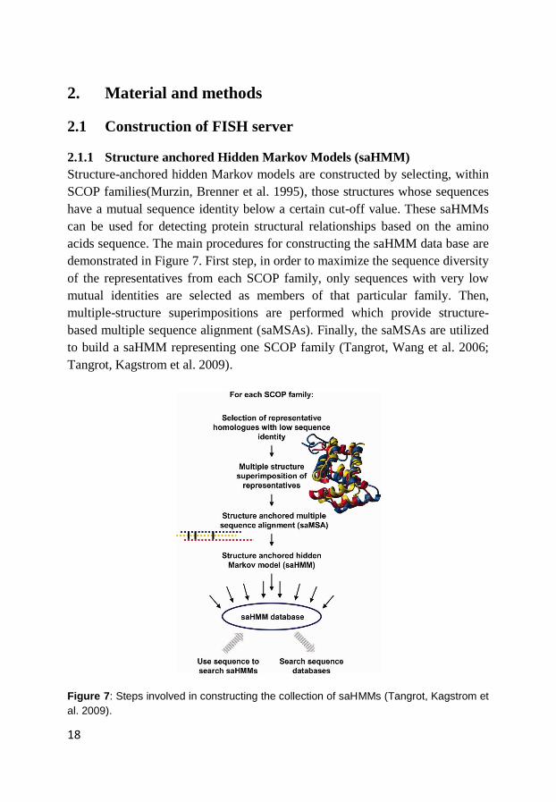
2.1.1 Structure anchored Hidden Markov Models (saHMM)

Structure-anchored hidden Markov models are constructed by selecting, within

SCOP families(Murzin, Brenner et al. 1995), those structures whose sequences

have a mutual sequence identity below a certain cut-off value. These saHMMs

can be used for detecting protein structural relationships based on the amino

acids sequence. The main procedures for constructing the saHMM data base are

demonstrated in Figure 7. First step, in order to maximize the sequence diversity

of the representatives from each SCOP family, only sequences with very low

mutual identities are selected as members of that particular family. Then,

multiple-structure superimpositions are performed which provide structure-

based multiple sequence alignment (saMSAs). Finally, the saMSAs are utilized

to build a saHMM representing one SCOP family (Tangrot, Wang et al. 2006;

Tangrot, Kagstrom et al. 2009).

Figure 7: Steps involved in constructing the collection of saHMMs (Tangrot, Kagstrom et

al. 2009).

19

2.1.2 Architecture of the FISH server

Figure 8: Schematic layout of the FISH server architecture. The user initializes a query

via the web interface. The query is processed by the query interpreter, using the

collection of saHMMs. The cross-link engine integrates information from the associated

data bases [SCOP, ASTRAL, PDB, nr (NCBI), Swiss-Prot and TrEMBL] with the results

of the query. The results assembler compiles the search results and presents them to

the user via the web interface.

Figure 8 shows an overview of architecture of the Fish server. At the heart of

the server lies a collection of 1050 saHMMs, which include all the saHMM

members. The individual saHMMs, saHMM-members, and corresponding

domain families were imported into a relational database (MySQL) and cross-

linked with other established databases which are locally available (see Figure

8).

The MySQL database is implemented on a Linux platform. The user interface is

written in Perl, PHP and JavaScript, and integrated with the Apache web server.

The user inputs a query via the web interface. The query interpreter processes

the input, using the collection of saHMMs. The cross-link engine merges

information from the associated databases with the results of the query. The

results assembler presents the outcome of the search to the user via the web

interface. The search results can be sent to the user by e-mail in the form of a

www-link and are stored on the server for 24 h.

20

2.2 Predicting protein order and disorder

2.2.1 Dataset

2.2.1.1 Training dataset

The training set was compiled by Pierre and colleagues (CHENG, et al., 2005).

It was used to train the DISpro protein predictor (Cheng, et al., 2005). This set

contains 215,612 residues, of which 13,909 (6.5%) are classified as disordered

as shown in Figure 9. Of the 13,909 disordered residues, 3,282 (23.6%) are part

of long regions of disorder (>30 AA) as shown in Table 1. These protein

sequences are extracted from the PDB, with the following constraints:

1. Crystal structures at higher than 2.5 Å resolution;

2. More than 30 amino acids in length;

3. Disordered regions at least 3 residues in length;

4. Sequence identity lower than 30%.

Figure 9: The composition of order and disordered amino acids in the training dataset.

Order94%

Disorder6%

21

Table 1: The composition of the long and short disordered regions in the training dataset.

Disordered length Regions Residues

Short(≤30aa) 1706 10627

Long(>30aa) 60 3282

2.2.1.2 Test datasets

Benchmark dataset For benchmarking, I use all 96 target sequences with known

structures available during CASP7. Residues in targets solved by Xray

crystallography were classified as disordered if no coordinates for the

crystallized residues were present. For targets solved by NMR, those residues

whose conformation was not sufficiently defined by NMR restraints, i.e.

exhibited high variability within the ensemble, or were annotated as disordered

in REMARK 465 by the experimentalists, were considered as disordered.

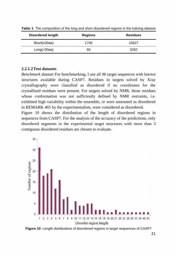
Figure 10 shows the distribution of the length of disordered regions in

sequences from CASP7. For the analysis of the accuracy of the predictions, only

disordered segments in the experimental target structures with more than 3

contiguous disordered residues are chosen to evaluate.

Figure 10: Length distributions of disordered regions in target sequences of CASP7

22

Blind test To facilitate performance comparison with other protein disorder

predictors, I used a blind test dataset that contains a balanced mixture of 80

sequences from fully ordered proteins and 79 fully disordered proteins. The

disordered regions were identified experimentally by methods other than X-ray

crystallography (Uversky, Gillespie et al. 2000). The fully ordered dataset was

annotated by PONDR® and is available from its website.

2.2.2 Conditional random fields (CRFs)

There are two kinds of models for building a probabilistic model for segment

and label sequence data: generative and discriminative models. Generative

models, such as Hidden Markov Models (HMMs) (Rabiner 1989), are based on

a model of the joint distribution p(y, x) where x and y are random variables

which range over the user supplied observation sequence that is to be labelled

and also over the corresponding sequence of labels. In order to define a joint

distribution sequence, all possible observation sequences must be enumerated

for a generative model. However, in most fields, this is difficult unless

observation elements are represented as isolated, independent from other

elements in an observation sequence. Therefore, HMMs require strict

independence assumptions over observation elements. However, most real-

world observation sequences contain multiple interacting features and long-

range dependencies between observation elements.

Our work employs discriminative models so called, conditional random fields

(CRFs) (Lafferty John, Andrew et al. 2001), which can overcome the drawbacks

of generative models. Conditional random field are powerful probabilistic

frameworks to label and segment sequential data. As a discriminative model,

CRFs directly model the conditional distribution p(y|x), and they do not need to

model the visible observation sequence x, which results in the relaxation of

strong independence assumptions over observation sequence. Moreover, CRFs

are able to model arbitrary features of observation sequences, regardless of the

relationships between them. Therefore, CRFs can overcome the inherent

shortcomings of generative models and achieve better labelling and prediction

performance.

23

Figure 11: Graphical structure of a chain-structured CRFs for sequences (Wallach

2004).

In case of chain-structured CRFs, which make a first-order Markov assumption

among label variables y that form a linear-chain, each label element of y has

access to any of the observation variables in x (see Figure 11).

More formally, let 𝒢 be an undirected model for x and y, then the fully

connected subgraphs define a set of cliques c c {{ , }}C x y . A CRF defines the

conditional probability of label sequence y given observation sequence x as:

1( | ) ( , ; ) (5)

( )c c

c C

p y x y xZ x

Where Φ is a real-valued potential function parameterized by λ, and

normalization factor

( ) ( , ) (6)c cy c CZ x y x

The potential function can be parameterized by an arbitrary set of feature

functions iF over each clique, a common form of which is

,( ; ) exp ( , ) (7)c c i i c c

i

y x F y x

The model is parameterized by a set of weights i { } , where each λi

weights the output of feature function iF . Note that in a first-order CRF,

24

cliques contain labels i i 1y , y and an arbitrary subset of observations from x.

Thus, the prediction for label yi is a function of the previous prediction yi-1 as

well as any number of features over the entire input sequence x.

In this study I use the CRF++ implementation for building CRF predictors.

CRF++, which is developed by Taku Kudo, is a simple, customizable, and open

source implementation of CRFs for segmenting and labeling sequenced data. It

was designed for generic purposes and can be applied to a variety of tasks. The

benefit of using CRF++ is that it enables us to redefine feature sets and specify

the feature templates in a flexible way (CRF++ is available at:

http://crfpp.sourceforge.net/).

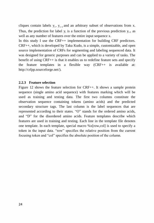
2.2.3 Feature selection

Figure 12 shows the feature selection for CRF++. It shows a sample protein

sequence (single amino acid sequence) with features marking which will be

used as training and testing data. The first two columns constitute the

observation sequence containing tokens (amino acids) and the predicted

secondary structure tags. The last column is the label sequences that are

represented according to their states. “O” stands for the ordered amino acids,

and “D” for the disordered amino acids. Feature templates describe which

features are used in training and testing. Each line in the template file denotes

one template. In each template, special macro %x[row,col] is used to specify a

token in the input data. “row” specifies the relative position from the current

focusing token and “col” specifies the absolute position of the column.

25

Figure 12: Feature selection of our models. A sliding window (size = 9) moves over the

protein sequence, and generates features according to the feature templates that

describes which features are used in training and testing.

2.2.4 Model building

2.2.4.1 Pruned CRF Model

Initially, training the CRFs model proved difficult due to a label imbalance

problem, since less than 6.5% of amino acids in the dataset are disordered. In

order to generate a more balanced training dataset, I keep only a limited number

of ordered amino acids that flank the disordered regions on both sides, and

prune the rest of the ordered sequence (see Figure 13). The rules for pruning

were determined after many rounds of optimization and are as follows: For

disordered regions, DRs, of less than or equal to 3 amino acids in length, DRs

≤ 3 aa., I keep one flanking amino acid on either side. Five flanking amino

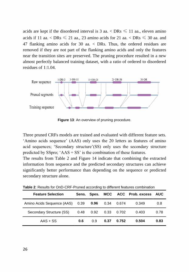
26

acids are kept if the disordered interval is 3 aa. < DRs ≤ 11 aa., eleven amino

acids if 11 aa. < DRs ≤ 21 aa., 23 amino acids for 21 aa. < DRs ≤ 30 aa. and

47 flanking amino acids for 30 aa. < DRs. Thus, the ordered residues are

removed if they are not part of the flanking amino acids and only the features

near the transition sites are preserved. The pruning procedure resulted in a new

almost perfectly balanced training dataset, with a ratio of ordered to disordered

residues of 1:1.04.

Figure 13: An overview of pruning procedure.

Three pruned CRFs models are trained and evaluated with different feature sets.

„Amino acids sequence‟ (AAS) only uses the 20 letters as features of amino

acid sequences; „Secondary structure‟(SS) only uses the secondary structure

predicted by SSpro; „AAS + SS‟ is the combination of these features.

The results from Table 2 and Figure 14 indicate that combining the extracted

information from sequence and the predicted secondary structures can achieve

significantly better performance than depending on the sequence or predicted

secondary structure alone.

Table 2: Results for OnD-CRF-Pruned according to different features combination

Feature Selection Sens. Spes. MCC ACC Prob. excess AUC

Amino Acids Sequence (AAS) 0.39 0.96 0.34 0.674 0.349 0.8

Secondary Structure (SS) 0.48 0.92 0.33 0.702 0.403 0.78

AAS + SS 0.6 0.9 0.37 0.752 0.504 0.83

27

Figure 14: Comparison of receive operating characteristic (ROC) curves based on

different feature combination.

By using 10-fold cross validation, I find that a window size of nine amino acids

results in the best template file for the feature subset selection. The optimal

value for the hyper-parameter “C” is 0.65, which trades the balance between

overfitting and underfitting. For all other parameters the default CRF++ values

are used.

Table 3: Results for the self consistency experiment.

Sequences Sens. Spec. Q2

Pruned 0.985 0.99 0.987

Original, Not-pruned 0.976 0.947 0.949

28

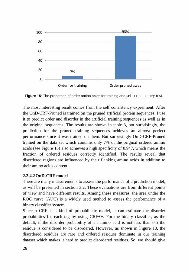
Figure 15: The proportion of order amino acids for training and self-consistency test.

The most interesting result comes from the self consistency experiment. After

the OnD-CRF-Pruned is trained on the pruned artificial protein sequences, I use

it to predict order and disorder in the artificial training sequences as well as in

the original sequences. The results are shown in table 3, not surprisingly, the

prediction for the pruned training sequences achieves an almost perfect

performance since it was trained on them. But surprisingly OnD-CRF-Pruned

trained on the data set which contains only 7% of the original ordered amino

acids (see Figure 15) also achieves a high specificity of 0.947, which means the

fraction of ordered residues correctly identified. The results reveal that

disordered regions are influenced by their flanking amino acids in addition to

their amino acids content.

2.2.4.2 OnD-CRF model

There are many measurements to assess the performance of a prediction model,

as will be presented in section 3.2. These evaluations are from different points

of view and have different results. Among these measures, the area under the

ROC curve (AUC) is a widely used method to assess the performance of a

binary classifier system.

Since a CRF is a kind of probabilistic model, it can estimate the disorder

probabilities for each tag by using CRF++. For the binary classifier, as the

default, if the disorder probability of an amino acid is not less than 0.5 the

residue is considered to be disordered. However, as shown in Figure 10, the

disordered residues are rare and ordered residues dominate in our training

dataset which makes it hard to predict disordered residues. So, we should give

7%

93%

0

20

40

60

80

100

Order for training Order pruned away

29

more advantages for predicting a disordered residue than for predicting an

ordered one. Therefore, instead of pruning the sequence, I adopt another

strategy to overcome the imbalance problem.

First, by using the 10-fold cross-validation, I find the best AUC value for the

OnD-CRF built on the training dataset. And then, the best operating point,

which gives the best trade off between sensitivity and specificity, is identified

according to ACC and Sw.

Based on the two steps, I find the best AUC value of 0.867 for the OnD-CRF

built on the training dataset and the best operating point which give rise to an

optimal P-value cut-off of P < 0.05 for ordered and P ≥ 0.05 for disordered

amino acids. Using this cut-off the OnD-CRF model achieves an ACC of 0.790

and a weighted score Sw of 0.580, respectively.

2.3 Predicting protein stability changes due to point mutations

In this study, for the classification task, I base our predictor on a three step

classification: destabilizing mutations (ΔΔG < −1.0 kcal/ mol), neutral

mutations (−1.0 kcal/mol ≤ ΔΔG ≤ 1.0 kcal/mol) and stabilizing mutations

(ΔΔG>1.0 kcal/mol).

2.3.1 Dataset and refinement

The dataset quality is important for building a reliable model. In recent studies

that used the training datasets S1615 (Capriotti, Fariselli et al. 2004) and S1948

(Capriotti, Fariselli et al. 2005) one found that these datasets contain a

significant percentage of redundant. After removing identical mutations that

were measured at the same temperature and pH value, Cheng et al. compiled a

redundancy-reduced dataset based on the dataset S1615. Kang et al. removed

the identical mutations if the sign of ΔΔG values conflicted and kept one if all

of them are of the same sign.

In this project, I compile a new dataset of protein mutation used for training and

testing which is derived from ProTherm (Oct 2009), with following constraints:

1) Considering only single point mutations.

2) The wild type protein structure must be deposited in the PBD.

3) The difference in free energy of unfolding is experimentally determined

by thermal denaturation.

4) All experimental conditions must be reported including the pH.

30

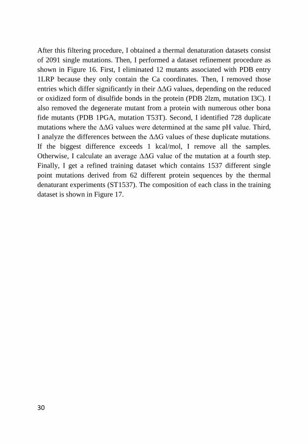
After this filtering procedure, I obtained a thermal denaturation datasets consist

of 2091 single mutations. Then, I performed a dataset refinement procedure as

shown in Figure 16. First, I eliminated 12 mutants associated with PDB entry

1LRP because they only contain the Ca coordinates. Then, I removed those

entries which differ significantly in their ΔΔG values, depending on the reduced

or oxidized form of disulfide bonds in the protein (PDB 2lzm, mutation I3C). I

also removed the degenerate mutant from a protein with numerous other bona

fide mutants (PDB 1PGA, mutation T53T). Second, I identified 728 duplicate

mutations where the ΔΔG values were determined at the same pH value. Third,

I analyze the differences between the ΔΔG values of these duplicate mutations.

If the biggest difference exceeds 1 kcal/mol, I remove all the samples.

Otherwise, I calculate an average ΔΔG value of the mutation at a fourth step.

Finally, I get a refined training dataset which contains 1537 different single

point mutations derived from 62 different protein sequences by the thermal

denaturant experiments (ST1537). The composition of each class in the training

dataset is shown in Figure 17.

31

2091 mutations from Protherm with PDB and ddG

2074 mutations

1346 different mutations728 identical mutations

669 mutation with slight

difference

(ddG difference < 1 kcal/mol)

After averaging 191 different

mutations1537 different mutations

1

2

3

4

5

Figure 16: The refinement procedure for the training dataset.

32

Figure 17: The composition of mutations according to the three classes.

Figure 18: Comparisons of amino acid frequencies considering the 20 amino acids. Blue

bars: the amino acid was replaced by any of the other 20 amino acids, e.g. Ala Xxx.

Red bar: this amino acids was used for mutation e.g. Xxx Ala.

Considering all 20 amino acids, as shown in Figure 18, the change of amino

acids to alanine is significantly more common than other mutations. This may

Destabilizing38%

Neutral53%

Stabilizing9%

0%

5%

10%

15%

20%

25%

30%

A R N D C E Q G H I L K M F P S T W Y V

Mutated

Mutation

33

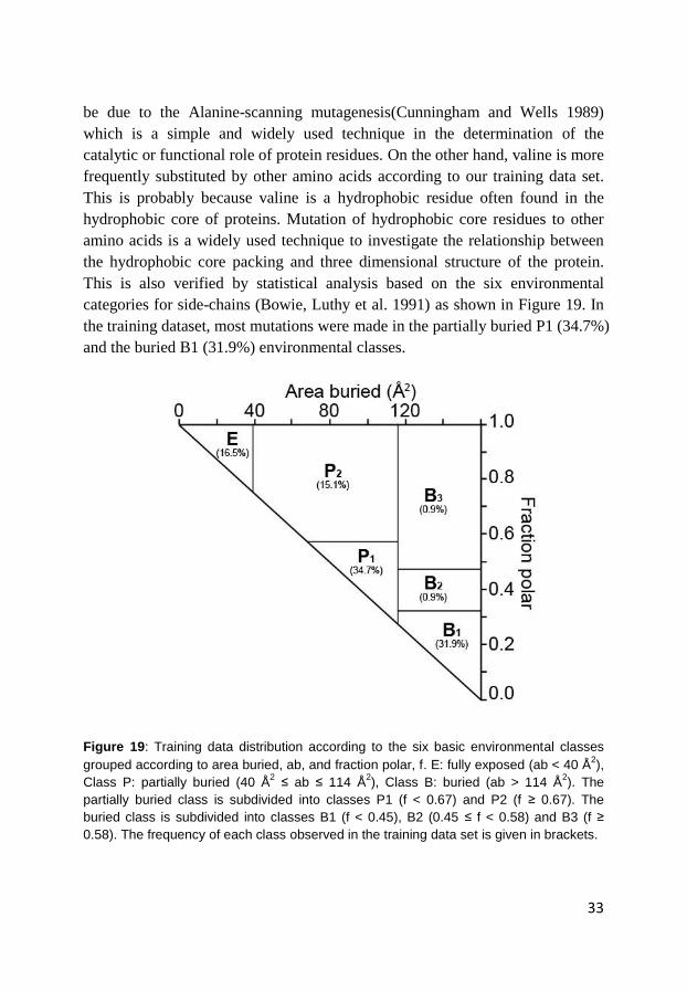
be due to the Alanine-scanning mutagenesis(Cunningham and Wells 1989)

which is a simple and widely used technique in the determination of the

catalytic or functional role of protein residues. On the other hand, valine is more

frequently substituted by other amino acids according to our training data set.

This is probably because valine is a hydrophobic residue often found in the

hydrophobic core of proteins. Mutation of hydrophobic core residues to other

amino acids is a widely used technique to investigate the relationship between

the hydrophobic core packing and three dimensional structure of the protein.

This is also verified by statistical analysis based on the six environmental

categories for side-chains (Bowie, Luthy et al. 1991) as shown in Figure 19. In

the training dataset, most mutations were made in the partially buried P1 (34.7%)

and the buried B1 (31.9%) environmental classes.

Figure 19: Training data distribution according to the six basic environmental classes

grouped according to area buried, ab, and fraction polar, f. E: fully exposed (ab < 40 Å2),

Class P: partially buried (40 Å2 ≤ ab ≤ 114 Å

2), Class B: buried (ab > 114 Å

2). The

partially buried class is subdivided into classes P1 (f < 0.67) and P2 (f ≥ 0.67). The

buried class is subdivided into classes B1 (f < 0.45), B2 (0.45 ≤ f < 0.58) and B3 (f ≥

0.58). The frequency of each class observed in the training data set is given in brackets.

34

2.3.2 Support vector machines (SVMs)

Support vector machines (SVMs) (Vapnik 1998) are the most important

algorithm in machine learning and have been successfully applied to a variety of

fields. In bioinformatics, SVMs have been widely applied to gene expression

data classification, protein 3D structure and function prediction (Cai, Liu et al.

2001) and protease function site recognition (Nanni and Lumini 2006).

The main idea of SVMs is to implicitly map data to a higher dimensional space

via a kernel function and perform classification through constructing a

maximum-margin hyperplane that optimally separates training data into two

classes. Figure 20 depicts an overview of the SVM process. When points are

separated by a nonlinear region as shown in the input space, SVMs use a kernel

function, K(x,y ) = Ø(x) × Ø(y) to calculate the dot product of Ø(x) and Ø(y)

implicitly, where x and y are input data points, Ø(x) and Ø(y) are the

corresponding data vectors in feature space, and Ø is the map from input space

to feature space. The mapped points become separable by a hyperplane in the

feature space. This hyperplane corresponds to a nonlinear curve in the original

input space.

Figure 20: An overview of the SVMs process

35

In the feature space, the two dashed lines correspond to the boundaries of two

classes respectively. The distance between the dashed lines is called the margin.

SVMs try to finds a hyperplane that is oriented so that the margin between the

support vectors is maximized. The vectors (points) that constrain the width of

the margin are the support vectors.

Originally, SVMs were developed for binary classification tasks. However,

most real life datasets are not binary classification. How to extend binary SVMs

to multi-class problem is still an on-going research. Several approaches were

constructed during the last few years. Although there are many sophisticated

approaches for multi-class SVMs, numerous experimental analysis have shown

that “One-Versus-ALL” (OVA) and “One-Versus-One” (OVO) are among the

most suitable methods for practical use.

Technically speaking, OVA is the simplest approaches for multi-class SVM. It

constructs K binary SVMs. The ith SVM is trained with all the samples from the

ith class against all the samples from the rest classes. Given a sample x to

classify, all the K SVMs are evaluated and the label of the class that has the

largest value of the decision function is chosen.

On the other hand, OVO is constructed by training binary SVMs between

pairwise classed. Therefore, an OVO model consists of K(K-1)/2 binary SVMs

for a K-class problem. Each of the K(K-1)/2 SVMs casts one vote for its

favoured class, and finally the class with most votes wins.

None of the multi-class implementation methods significantly outperforms the

others in terms of classification accuracy. The difference mainly lies in the

training time, evaluation speed and the size of the trained classifier model. For

example, as for the training time, although OVA only require K binary SVM, its

training is computationally most expensive because each binary SVM is

optimized on all the N training samples. OVO has K(K-1)/2 binary SVMs to

train, which seems much more than OVA need. However, each SVM is trained

ON 2N/k samples. The overall training speed is significantly faster than OVA.

Thus, in this study, I apply the OVO for the 3-state classification SVM because

the OVO approach can achieve better prediction accuracy and faster cross-

validation speed.

The libsvm (http://www.csie.ntu.edu.tw/~cjlin/libsvm/) support vector machine

package is used to build the 3-state classification and regression predictors. The

radial basis function (RBF) [exp (-gamma*|u-v|2)], which is a non-linear kernel

function, is used. The kernel parameters are obtained by cross-validation. The

cost parameter, C, controls the trade off between allowing training errors and

36

forcing rigid margins. It creates a soft margin that permits some

misclassifications. Increasing the value of C increases the cost of misclassifying

points and forces the creation of a more accurate model that may not generalize

well. The Gaussian width, gamma, is the inverse of the variance of the RBF.

The larger the value for gamma, the more peaked the Gaussians become around

the support vectors, and therefore the more complex the decision boundary can

be. Smaller gamma corresponds to a smoother decision boundary (Schölkopf,

Tsuda et al. 2004).

2.3.3 Feature selection

In order to investigate what information could affect the prediction accuracy of

protein stability changes, three different input and encoding strategies are

proposed: sequence-generated information only (SeqOnly), structure-generated

information only (StruOnly) and the combinations of sequence and structure

(Stru&Seq). All strategies include the experimental pH values. Different from

many previously published methods, I do not consider the experimental

temperature since it is one of the variables for thermal denaturation experiments.

For the SeqOnly strategy, the features are extracted as follow:

i) I incorporate information derived from the protein sequence by encoding

local amino acid composition of the partial wild type and mutated sequences

within an input window (size=31) centred on the mutated residue, which

includes the frequencies of each 20 amino acid, and the frequency for the spacer

character which needs to be introduced at N- and C- terminus of the protein.

ii) The physicochemical z-scales, three for a particular amino acid of the WT

protein, and three for the mutated protein, resulting in 3×2=6 z-scales for each

position. The z-scales are based on 29 principal physicochemical properties of

the amino acids, and are used to describe the deleted and the introduced amino

acids (Hellberg, Eriksson et al. 1991; Sjostrom, Rannar et al. 1995).

iii) Similar to z-scales, I derive e-scales by principle components analysis (PCA)

of the 3D-1D scoring table that contains measurements of the compatibilities of

the twenty amino acids with the eighteen environmental classes. In other words,

one maps the 20 amino acids onto the 18 environmental classes. These 18

classes include the three secondary structure states (helix, strand, loop) in

addition to the six environmental classes mentioned in Fig. 19 (Bowie, Luthy et

al. 1991). The e-scales reflect the most important compatible properties of an

amino acid, such as volume, hydrophilicity and charge.

Considering all the above, the SeqOnly method has a total of 55 inputs.

37

Most of the previously published methods, such as I-mutant2 (Capriotti,

Fariselli et al. 2005), Mupro (Cheng, Randall et al. 2006) and AutoMute (Masso

and Vaisman 2008), utilize tertiary structure information for the prediction of

stability changes. These methods use the frequency of each type of residue

within a sphere of 9 Å or 12 Å radiuses (between the Cα atoms) around the

target mutated residue as input feature. The limitation of such sphere models is

that they ignore the size, shape and orientation of amino acids, and in general do

not take into account the atomic groups that surrounding the mutated amino

acids. Figure 21 shows the neighbouring atomic groups of N101 in the T4

lysozyme protein (PDB entry 2LZM). The Cα distance between N101 and Y161

is more than 12 Å. However, the oxygen atom of the side chain of N101 is close

to OH of Y161. In order to avoid these limitations for the StruOnly strategy, I

extracted the features as follow:

i) for the first set of 26 (13×2) inputs, I define the packing densityix for each of

the 13 atomic groups (N3H0, N3H1, N3H2, N4H3, O1H0, O2H1, C3H0, C3H1,

C4H1, C4H2, C4H3, S2H0, S2H1) (Tsai, Taylor et al. 1999) surrounding the

side-chain and main-chain of mutated amino acid as:

chain=mainchain4

(8)

chain=sidechain

i

i

x

i

xif

xif

N

When considering the main-chainix , I sum each of the 13 atomic groups of

other-residues at distances less than 4 Å and then divide those numbers by 4

since there are four atomic groups (N3H1, C4H1, C3H0, and O1H0) on the

main-chain. For side-chainix , I add the number of each 13 atomic groups of

other-residue at distances smaller than 4 Å and then divide those numbers by N

which is the overall side-chain atomic groups.

In the general labels XnHm, X stands for the atom type of the non-hydrogen

atom, n its valence; Hm, the number m of hydrogen atoms attached to the atom.

E.g. C3H1 is a trigonal carbon atom with one attached hydrogen (Tsai, Taylor et

al. 1999).

ii) I include a further 12 inputs: the number of hydrogen bonds which surround

the side chain of the mutated amino acid (1 input), the six basic environmental

38

classes determined from the area of the side chain that is buried in the protein

and by the fraction of the side chain area that is exposed to polar atoms (6

inputs), the fractional accessible surface area (ASA) of side chain (1 input) and

the secondary structure of mutated the amino acids (4 inputs; helix, strand, coil

and turn). All these inputs are calculated by the VADAR program package

(Willard, Ranjan et al. 2003) from the wild type structure.

iii) The mutation information consist of 20 inputs which code for the 20

different amino acids. The input corresponding to the mutated residue type is set

to -1 and the input corresponding to the introduced residue type is set to +1. All

other inputs are set to 0.

Considering all inputs, the StruOnly method includes a total of 59 inputs.

For the Stru&Seq strategy, all sequence-generated information and structure-

generated information are combined except the 20 inputs which code for the 20

different amino acids. Finally, I obtain 94 inputs for Stru&Seq method.

Figure 21: Neighboring atomic groups of N101 in the T4 lysozyme protein (PDB entry

2LZM).

39

2.3.4 Non-clustered model

2.3.4.1 Three-state classification

In the non-clustered model we include all protein sequences in the training data

set regardless to which protein family they belong.

As shown in Table 4, combining the structure and sequence information,

(Stru&Seq model) increases the overall accuracy, ACC, by ~1.5 percent and

correlation coefficient, CC, by ~2.2 percent compared to the SeqOnly model. It

can also be seen that, the prediction accuracy of the SeqOnly model is slightly

better compared to the StruOnly model. This indicates that, for non-clustered

model, the protein sequences alone carry the necessary information for

predicting the change of protein stability. The higher the sequence identity or

the more similar the structures and function are, the better prediction results will

be achieved.

Table 4: 20-fold cross-validation on datasets ST1537 for 3-state classification of non-

clustered model

Method ACC[-] ACC[N] ACC[+] ACC CC

Stru&Seq 0.738 0.85 0.502 0.776 0.678

SeqOnly 0.739 0.827 0.484 0.761 0.656

StruOnly 0.693 0.815 0.438 0.73 0.58

Further, I noticed that the prediction of destabilizing and neutral mutation

achieve significantly better performance than the prediction accuracy of

stabilizing mutations. Considering the composition of the training datasets

based on the three classes, as shown in Figure 17, I believe this is due to the

uneven proportion of the samples of the three classes in the training datasets.

This is reasonable since it‟s harder to make protein more stable in general. On

the other hand, it means that the prediction for stabilizing mutation is still a

challenging task.

2.3.4.2 Predicting directly the values of the free energy changes (ΔΔG)

Figure 22 displays the relationship between the experimental and predicted

values of ΔΔG for the training dataset using SVM regression with Stru&Seq

method. As shown in Table 5, the performance of the regression models are

evaluated by correlation coefficient (CC), Mean Absolute Error (MAE) and

40

Standard Error of estimate (ζest). The correlation coefficient (CC) reaches values

over 0.80 for both Stru&Seq and SeqOnly method. And, when based on the

Stru&Seq method, the best MAE and ζest reach 0.665 and 1.05, respectively.

Figure 22: The correlation between the experimental and predicted values based on the

Stru&Seq method is very good.

Table 5: Results of the 20-fold cross-validation on dataset ST1537 for regression

Method CC MAE σest

Stru&Seq 0.825 0.665 1.05

SeqOnly 0.8 0.699 1.11

2.3.4.3 Prediction accuracy according to environmental class

Table 6 reports the prediction accuracy for stabilizing, neutral and destabilizing

mutations with regard to the six basic environment classes. The predicting

model was built according to the Stru&Seq scheme.

y = 0.6792x - 0.2718

-14

-12

-10

-8

-6

-4

-2

0

2

4

6

-20 -15 -10 -5 0 5 10

Pre

dic

ted

ΔΔG

Experimental ΔΔG

41

Table 6: The prediction accuracy of the training datasets based on the six environmental

classes

Enverimental class ACC[-] ACC[N] ACC[+] ACC

E0 0.73 0.87 0.5 0.8

P2 0.66 0.88 0.44 0.77

P1 0.73 0.82 0.48 0.75

B3 1 1 0.67 0.93

B2 0.75 1 0 0.86

B1 0.78 0.85 0.56 0.79

The experimental mutation under the environmental classes B2 and B3 are rare

(See Figure 19). From a biological point of view, this is probably due to the low

frequency of amino acids found in a buried and at the same time polar

environment. Analyzing the results of the other four environmental classes, I

noticed that most experimental mutations carried out in the B1and P1

environments, achieve best performance for both stabilizing and destabilizing

mutations.

2.3.5 Clustered model for 3-state classification

In order to investigate the prediction accuracy for the proteins that are not

included in our training dataset, we cluster the training data set sequences

according to the SCOP family definition (Murzin, Brenner et al. 1995). The 62

proteins are clustered together into 47 families, as shown in Figure 23. The

prediction results after 47-fold cross validation are listed in Table 7. The overall

accuracy and correlation of the predictions for protein sequences that are not

homologous to any of the training data set sequences are 0.63 and 0.37,

respectively. Both values are significantly lower than the values obtained from

the not-clustered method. This is due to the fact that when one performs 20-fold

cross validation on the non-clustered data, there are many homologues or

protein differing by just one mutation, contained in the training and test datasets.

Table 7: Results of 47-fold cross-validation on dataset ST1537 for 3-state classification

of the clustered model

Method ACC[-] ACC[N] ACC[+] ACC CC

Stru&Seq 0.54 0.78 0.09 0.63 0.37

SeqOnly 0.54 0.70 0.04 0.58 0.29

StruOnly 0.52 0.79 0.11 0.62 0.33

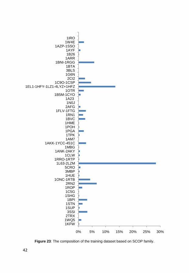
42

Figure 23: The composition of the training dataset based on SCOP family.

0% 5% 10% 15% 20% 25% 30%

1KFW1WQ52TRX3SSI

1SUP1STN1BPI

1SHG1C5G1ROP2RN2

1ONC-1RTB1HUE3MBP5CRO

1L63-2LZM1RRO-1RTP

1CLW1ANK-2AKY

1MBG1AKK-1YCC-451C

1AM71TPK1PGA1POH1HME1BVC1RN1

1FLV-1FTG2AFG1N0J1A23

1B5M-1CYO1OTR

1EL1-1HFY-1LZ1-4LYZ+1HFZ1C9O-1CSP

2CI21G6N3BLS1BTA

1BNI-1RGG1ARR1B261AYF

1AZP-1SSO1W4E1IRO

43

3. Evaluation criteria

3.1 Cross validation

In machine learning community, cross-validation is a commonly used and

widely accepted technique for estimating the generalization performance, model

comparison and optimizing learning model parameters.

3.1.1 Procedures of cross-validation

Hold-Out Validation This method randomly split the available data into a

training dataset and a test dataset. Generally, the testing data is less than a third

of the initial data. The model is trained on the training dataset, and predictive

performance is assessed using the testing data. Hold-out validation avoids the

overlap between training data and test data, yielding a more accurate estimate

for the generalization performance of the algorithm. The drawback is that this

procedure does not use all the available data and the results are highly

dependent on the choice for the training/test split.

K-fold cross validation In this approach, the data is randomly partitioned into k

equally (or nearly equally) sized subsets or folds. Of the k subsets, a different

single subset is held-out as the test data for testing the model, and the remaining

k−1 subsets are used for learning. The cross-validation process is then repeated

k times (the folds), with each of the k subsets used exactly once as the test data.

The k results from the folds then can be averaged to produce a single estimation.

Leave-One-Out Cross-validation Leave-One-Out cross-validation is a special

case of k-fold cross-validation where k is the number of data points. Leave-

one-out cross validation is useful because it does not waste data. When training,

all but one of the points are used, so the resulting regression or classification

rules are essentially the same as if they had been trained on all the data points.

The main drawback to the leave-one-out method is that it is expensive - the

computation must be repeated as many times as there are training set data points.

3.1.2 Key Application

Performance estimation Cross-validation can be used to estimate many

performance measurements such as accuracy, sensitivity, specificity, or

correlation. For example, using 10-fold cross-validation, one repeatedly uses 90%

of the data to build a model and test its accuracy on the remaining 10%. The

resulting average accuracy is likely to be somewhat of an underestimate for the

44

true accuracy when the model is trained on all data and tested on unseen data,

but in most cases this estimate is reliable, particularly if the amount of labelled

data is sufficiently large and if the unseen data follows the same distribution as

the labelled examples.

Model comparison Different predictors may use the cross-validation to compare

the predictive performance on some benchmark datasets.

Optimizing Many classifiers are parameterized and their parameters can be

tuned to achieve the best result with a particular dataset. For example, support

vector machines (SVM) use soft-margins to deal with noisy data. There is no

easy way of learning the best value for the soft margin parameter for a particular

dataset other than trying it out and seeing how it works. In such cases, cross-

validation can be performed on the training data as to measure the performance

with each value being tested. Alternatively a portion of the training set can be

reserved for this purpose and not used in the rest of the learning process. But if

the amount of labelled data is limited, this can significantly degrade the

performance of the learned model and cross-validation may be the best option.

3.2 Assessment of classification

3.2.1 Sensitivity and specificity

For binary predictions, sensitivity (Sens.) and specificity (Spec.) are commonly

used to evaluate predictive accuracy. Sens. and Spec. are defined in the

following equations:

(9)TP

TP FN

NSensitivity

N N

(10)TN

TN FP

NSpecificity

N N

In the disorder prediction, sensitivity represents the fraction of disordered

residues correctly identified in a prediction, while specificity indicates the

fraction of ordered residues correctly identified. NTP is true positive (residues

predicted and observed disordered). NFN is false negative (residues predicted

ordered but in fact disordered). NTN is true negative (residues predicted and

observed ordered). NFP is false positive (residues predicted disordered by

observed ordered).

45

3.2.2 ROC curve

The Receiver Operating Characteristic (ROC) curve is a two dimensional

measure of classification performance. It shows a classifier‟s performance as a

trade off between specificity and sensitivity.

The area under the ROC curve (AUC) is a convenient way of comparing

classifiers. A random classifier has an area of 0.5, while an ideal one has an area

of 1.

The operating point, usually a classifier, is used at a particular sensitivity, or at a

particular threshold. The ROC curve can be used to choose the best operating

point which lies on the classifier's ROC. The best operating point might be

chosen so that the classifier gives the best trade off between the costs of failing

to detect positives against the costs of raising false alarms. The best place to

operate the classifier is the point on its ROC which lies on a 45 degree line

closest to upper left corner (0, 1) of the ROC plot.

3.2.3 S-product, Sw and ACC

In order to reward the predictors more generously for correctly predicting a

disordered residue than for predicting an ordered one, in the evaluation of

CASP disorder prediction, S-score (Sw) is introduced(Jin and Dunbrack 2005;

Bordoli, Kiefer et al. 2007).

(11)d TP o FP o TN d FNw

d d o o

W N W N W N W NS

W N W N

Where Nd and No are the total number of residues observed as disordered and

ordered, respectively. Wd and Wo are weights assigned to experimentally

defined disordered and ordered residues.

To combine both sensitivity and specificity to a single measurement, the S-

product and ACC are defined as follow:

(12)productS Sens Spec

(13)2

Sens SpecACC

46

3.2.4 Matthews’ correlation coefficient

In machine learning, Matthews‟s correlation coefficient (MCC) is a

measurement for the quality of binary classifications. The MCC is defined as

follow:

(14)( )( )( )( )

TP TN FP FN

TP FP TP FN TN FP TN FN

N N N NMCC

N N N N N N N N

3.3 Assessment of Regression

3.3.1 Pearson's correlation

For protein stability prediction, the Pearson correlation coefficient (CC) is used

to determine the relationship between the predicted and experimental ΔΔG by

following equation:

2 2

( )( ) (15)

( ) ( )

x x y yCC

x x y y

For the protein stability prediction, x and y are the predicted and experimental

ΔΔG values, respectively. x and y are the sample means of the predicted and

experimental ΔΔG.

3.3.2 Mean absolute error (MAE) and the standard error of estimate

For SVM regression, the performance is also evaluated using the mean absolute

error (MAE) and the Standard error (ζest):

1

1 (16)

n

i i

i

MAE x yn

Here, ix is the prediction and iy is the experimental value. And, n is the number

of all mutations from dataset.

2( ) (17)est

y x

n

Here, y is an experimental value, x is a predicted values. The numerator is the

sum of squared differences between the experimental values and the predicted

values, and n is the number of pairs of scores.

47

4. Contributions and relate works

4.1 Construction of FISH server (Paper I, II)

In this work, the FISH server for the identification of sequence homologues on

the basis of protein domains has been developed. It is not only able to compare

a query sequence with all structure anchored hidden Markov models (saHMMs)

assign family membership on the domain level, but also can be used to discover

those proteins in a database that harbour a certain domain, independent of

sequence identity and annotation status. Moreover, the cross-link between

saHMM database and other biological databases, such as SCOP, PDB,

ASTRAL, SwissProt and TrEMBL, has been established on the server (see

Figure 24 and Figure 25). This could facilitate further exploration of the

structure and function of the query sequence.

Figure 24: Schematic view of the database cross-linking used in the FISH server

48

Figure 25: The layout of the FISH server.

4.2 Prediction of order and disorder in proteins (Paper III)

Two strategies for predicting order and disorder in proteins using conditional

random fields have been developed. I compare our two predictors (OnD-CRF-

Pruned and OnD-CRF) to fifteen previously developed protein disorder

predictors over CASP7 benchmarking dataset. Evaluation is done with respect

to the AUC, the sensitivity, Ssens, the specificity, Sspec, their product, Sprod,

the ACC and Sw. The sensitivity and specificity are interpreted as the fraction

of correctly identified disordered and ordered residues, respectively. The

49

benchmarking results for all 17 disorder prediction methods are listed in Table 8.

The comparison is divided into the fully automated server group and the human

expert group. The main difference between the categories is human groups can

make use of expertise of a knowledgeable human and time to interpret the

automated method's results while preparing their nonautomated predictions for

CASP.

Within the automatic server group, both our methods achieve better overall

performance for AUC, Sprod, ACC and Sw as well as the Sens. The performance

of OnD-CRF method is comparable to the best human expert methods, such as

ISTZORAN and fais. The results show, that OnD-CRF and OnD-CRF-Pruned

are accurate and effective methods for the fully automated prediction of

disorder in proteins.

Table 8: Comparing OnD-CRF and OnD-CRF-Pruned with prediction methods that

participated in CASP7.

Method AUC Ssens Sspec Sprod ACC Sw

CASP7 Automatic Server Group

OnD-CRFa 0.84 0.69 0.81 0.56 0.75 0.5

OnD-CRF-Pruned 0.81 0.62 0.85 0.53 0.74 0.47

DISproa 0.82 0.6 0.85 0.51 0.73 0.45

GeneSilicoMetaServerd 0.8 0.53 0.91 0.48 0.72 0.44

BIME@NTU_serva 0.8 0.59 0.84 0.5 0.72 0.43

DISOPREDa 0.84 0.43 0.95 0.41 0.69 0.38

Distilla 0.72 0.56 0.79 0.44 0.67 0.35

MBI-NTU-serva 0.8 0.33 0.97 0.32 0.65 0.3

DRIPPREDb 0.76 0.38 0.91 0.35 0.65 0.29

CASP7 Human Expert Group

ISTZORANb 0.86 0.73 0.84 0.61 0.78 0.56

faisa 0.84 0.56 0.92 0.51 0.74 0.48

CBRC-DRa 0.85 0.45 0.97 0.44 0.71 0.42

BIME@NTUc 0.8 0.54 0.88 0.47 0.71 0.42

IUPredb 0.78 0.4 0.95 0.38 0.67 0.34

CBRC-DP_DRa 0.7 0.34 0.97 0.33 0.66 0.31

Okab 0.61 0.28 0.94 0.26 0.61 0.22

Softberrya 0.7 0.2 0.97 0.2 0.59 0.17

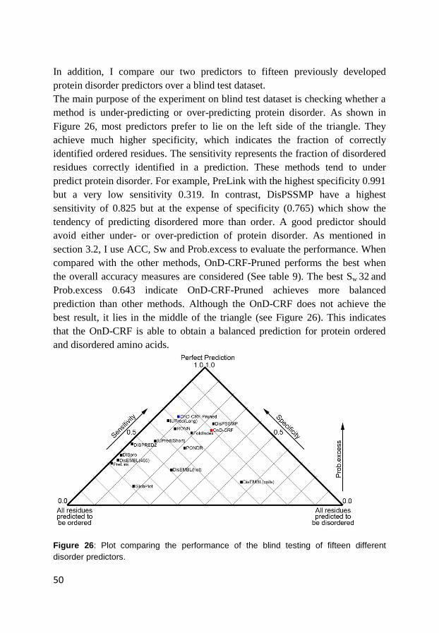
50

In addition, I compare our two predictors to fifteen previously developed

protein disorder predictors over a blind test dataset.

The main purpose of the experiment on blind test dataset is checking whether a

method is under-predicting or over-predicting protein disorder. As shown in

Figure 26, most predictors prefer to lie on the left side of the triangle. They

achieve much higher specificity, which indicates the fraction of correctly

identified ordered residues. The sensitivity represents the fraction of disordered

residues correctly identified in a prediction. These methods tend to under

predict protein disorder. For example, PreLink with the highest specificity 0.991

but a very low sensitivity 0.319. In contrast, DisPSSMP have a highest

sensitivity of 0.825 but at the expense of specificity (0.765) which show the

tendency of predicting disordered more than order. A good predictor should

avoid either under- or over-prediction of protein disorder. As mentioned in

section 3.2, I use ACC, Sw and Prob.excess to evaluate the performance. When

compared with the other methods, OnD-CRF-Pruned performs the best when

the overall accuracy measures are considered (See table 9). The best Sw 32 and

Prob.excess 0.643 indicate OnD-CRF-Pruned achieves more balanced

prediction than other methods. Although the OnD-CRF does not achieve the

best result, it lies in the middle of the triangle (see Figure 26). This indicates

that the OnD-CRF is able to obtain a balanced prediction for protein ordered

and disordered amino acids.

Figure 26: Plot comparing the performance of the blind testing of fifteen different

disorder predictors.

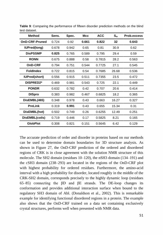
51

Table 9: Comparing the performance of fifteen disorder prediction methods on the blind

test dataset.

Method Sens. Spec. Mcc ACC Sw Prob.excess

OnD-CRF-Pruned 0.724 0.92 0.661 0.822 32 0.643

IUPred(long) 0.678 0.942 0.65 0.81 30.9 0.62

DisPSSMP 0.825 0.765 0.589 0.795 29.4 0.59

RONN 0.675 0.888 0.58 0.7815 28.2 0.563

OnD-CRF 0.794 0.751 0.544 0.7725 27.1 0.545

FoldIndex 0.722 0.815 0.54 0.7685 26.68 0.536

IUPred(short) 0.556 0.915 0.511 0.7355 23.5 0.472

DISPRED2* 0.469 0.981 0.543 0.725 22.1 0.449

PONDR 0.632 0.782 0.42 0.707 20.6 0.414

DISpro 0.383 0.982 0.467 0.6825 18.2 0.365

DisEMBL(465) 0.348 0.978 0.43 0.663 16.27 0.327

PreLink 0.319 0.991 0.43 0.655 15.34 0.31

DisEMBL(hot) 0.502 0.749 0.26 0.6255 12.49 0.251

DisEMBL(coils) 0.719 0.446 0.17 0.5825 8.21 0.165

GlobPlot 0.308 0.821 0.151 0.5645 6.42 0.129

The accurate prediction of order and disorder in proteins based on our methods

can be used to determine domain boundaries for 3D structure analysis. As

shown in Figure 27, the OnD-CRF prediction of the ordered and disordered

regions of CRK is in close agreement with the solution NMR structure of this

molecule. The SH2 domain (residues 10–120), the nSH3 domain (134–191) and

the cSH3 domain (238–293) are located in the regions of the OnD-CRF plot

with highest probability for ordered residues. Furthermore, the amino-acid

interval with a high probability for disorder, located roughly in the middle of the

CRK-SH2 domain, corresponds precisely to the highly dynamic loop (residues

65–85) connecting the βD and βE strands. The DE-loop changes its

conformation and provides additional interaction surface when bound to the

regulatory SH3 domain of Abl. (Donaldson et al., 2002). This is remarkable

example for identifying functional disordered regions in a protein. The example

also shows that the OnD-CRF trained on a data set containing exclusively

crystal structures, performs well when presented with NMR data.

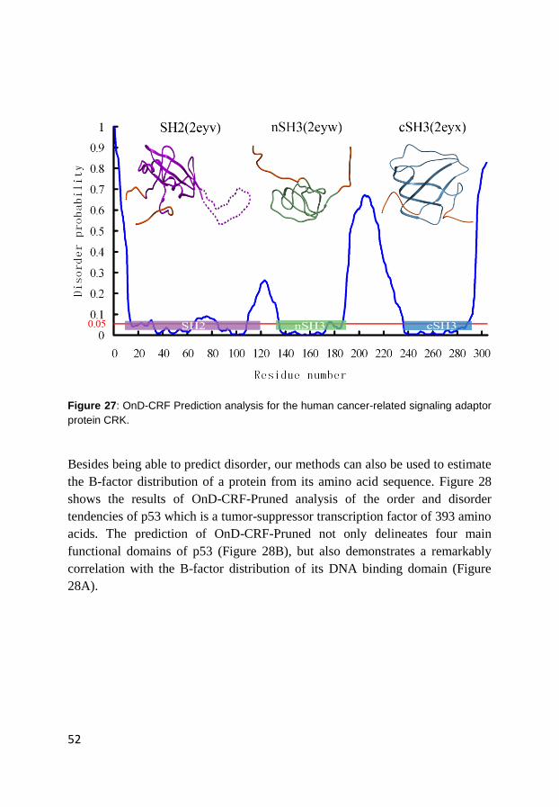
52

Figure 27: OnD-CRF Prediction analysis for the human cancer-related signaling adaptor

protein CRK.

Besides being able to predict disorder, our methods can also be used to estimate

the B-factor distribution of a protein from its amino acid sequence. Figure 28

shows the results of OnD-CRF-Pruned analysis of the order and disorder

tendencies of p53 which is a tumor-suppressor transcription factor of 393 amino

acids. The prediction of OnD-CRF-Pruned not only delineates four main

functional domains of p53 (Figure 28B), but also demonstrates a remarkably

correlation with the B-factor distribution of its DNA binding domain (Figure

28A).

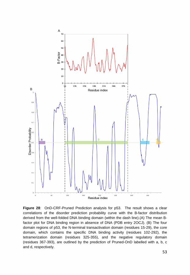
53

Figure 28: OnD-CRF-Pruned Prediction analysis for p53. The result shows a clear

correlations of the disorder prediction probability curve with the B-factor distribution

derived from the well-folded DNA binding domain (within the dash line).(A) The mean B-

factor plot for DNA binding region in absence of DNA (PDB entry 2OCJ). (B) The four

domain regions of p53, the N-terminal transactivation domain (residues 15-29), the core

domain, which contains the specific DNA binding activity (residues 102-292), the

tetramerization domain (residues 325-355), and the negative regulatory domain

(residues 367-393), are outlined by the prediction of Pruned-OnD labelled with a, b, c

and d, respectively.

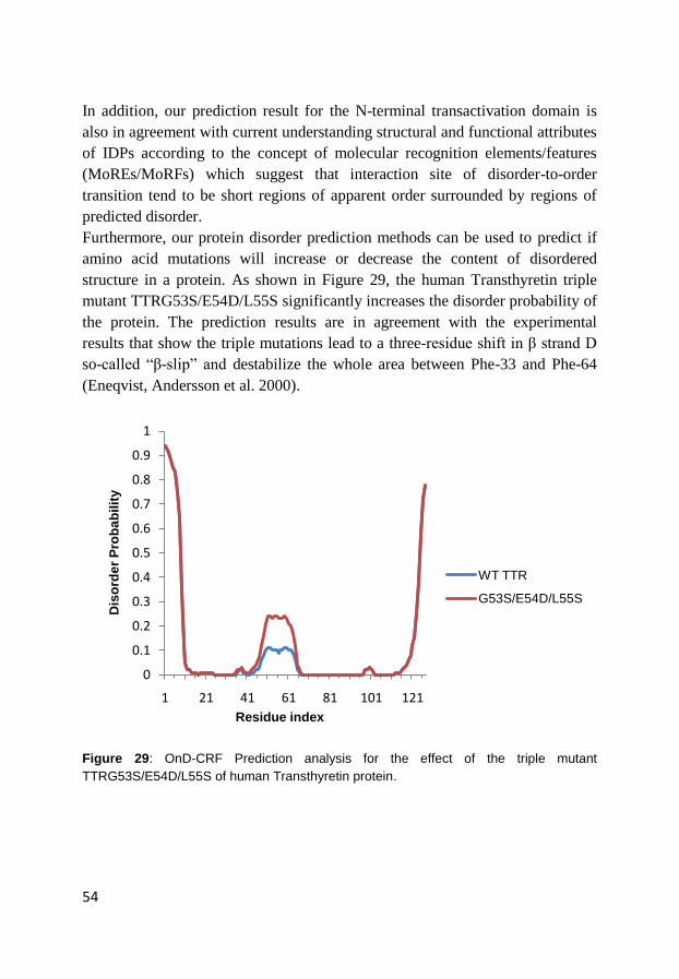
54

In addition, our prediction result for the N-terminal transactivation domain is

also in agreement with current understanding structural and functional attributes

of IDPs according to the concept of molecular recognition elements/features

(MoREs/MoRFs) which suggest that interaction site of disorder-to-order

transition tend to be short regions of apparent order surrounded by regions of

predicted disorder.

Furthermore, our protein disorder prediction methods can be used to predict if

amino acid mutations will increase or decrease the content of disordered

structure in a protein. As shown in Figure 29, the human Transthyretin triple

mutant TTRG53S/E54D/L55S significantly increases the disorder probability of

the protein. The prediction results are in agreement with the experimental

results that show the triple mutations lead to a three-residue shift in β strand D

so-called “β-slip” and destabilize the whole area between Phe-33 and Phe-64

(Eneqvist, Andersson et al. 2000).

Figure 29: OnD-CRF Prediction analysis for the effect of the triple mutant

TTRG53S/E54D/L55S of human Transthyretin protein.

0

0.1

0.2

0.3

0.4

0.5

0.6

0.7

0.8

0.9

1

1 21 41 61 81 101 121

Dis

ord

er

Pro

ba

bil

ity

Residue index

WT TTR

G53S/E54D/L55S

55

4.3 Prediction of protein mutation-induced stability change

(Paper IV)

In the last manuscript, I describe a method for predicting protein stability

changes due to single mutation, called ProSMS.

The ability to predict a protein‟s tolerance to amino acid substitutions is of

fundamental importance to understand natural protein evolution, for developing

protein engineering strategies, and for understanding the basis of genetic

diseases (Bloom, Silberg et al. 2005). In contrast to the common binary

predictors, I base our predictors on a three-state classification which introduces

in addition to the destabilizing mutations (ΔΔG < −1.0 kcal/ mol) and

stabilizing mutations (ΔΔG > 1.0 kcal/mol), as a third class the neutral

mutations (−1.0 kcal/mol ≤ ΔΔG ≤ 1.0 kcal/mol).

Moreover, based on a refined training dataset, I propose non-clustered and

clustered models for a three-state classification of protein stability changes

resulting from single amino acid mutation. Results for the non-clustered model

(see Table 4) indicate that that the prediction accuracy based only on the protein

sequence information is comparable to the accuracy when protein structure

information is included. However, for clustered model, the prediction accuracy

is significantly improved when protein tertiary structure information, in form of

local environmental conditions, are available.

From comparing the prediction accuracies of the non-clustered and the clustered

models we can conclude, that many established predictors appear to be more

accurate than they actually are. They perform well on sequences that are

homologous to sequences in the training data set, but perform worse on non-

homologous sequences. The reason is that due to the traditional k-fold cross

validation, they can only estimate the prediction ability for query proteins that

are homology related to proteins in their training datasets. Confronted with a

novel sequence, without homologue in the training data set, they will not be

able to achieve high accuracy.

The predictive model based on the 47-fold cross validated clustered training

data set, provides a realistic estimate of the lower bound for predictions, since

none of the query sequences were used for training the model.

The predictive ability of our 3-state model is then compared with the method

developed by Capriotti et al., who adopted a hypothesis of thermodynamic

reversibility of the existing experimental data, and using cross validation on 20

sub datasets which were clustered according to their sequence similarity using

56

the blastclust program in the BLAST suite. For the 3-state classification, the

best SVMs method (SVM-3D9) achieves an accuracy of 61% with a correlation

coefficient of 0.35. Our method can predict the 3-state of protein mutants with

an accuracy of 78% and a correlation of 0.68 for non-clustered model with 20-

fold cross validation, and an accuracy of 63% and a correlation of 0.37 with 47-

fold cross validation for clusterd model. Although direct comparison is not

appropriate due to the difference of datasets used in for training and test, I use a

refined experimental dataset and more elaborate cross-validation, the significant

improvement in accuracy and correlation indicates that our method is better and

more reliable.

I also compare the performance of predicting the actual free energy changes

resulting from mutation and 2-state classification by the S1948 dataset which

was used by AutoMute(Masso and Vaisman, 2008). The results are shown in

Table 10.

Table 10: Comparison of regression algorithms over S1948 dataset.

Method CC σest Regression line

ProSMS-Stru&Seq 0.9 0.9 y=0.777x-0.212

AUTO-MUTE-REPTree 0.8 1.1 y=0.5357x−0.4376

Capriotti (SVMreg) 0.7 1.3 y=0.5223x−0.4705

Based on the 20-fold cross-validate results, the correlation coefficient and the

standard error of our ProSMS method is with 0.9 and 0.9, respectively,

significantly better than the AUTO-MUTE-REPTree and Capriotti

(SVMreg)(Capriotti, et al., 2005).

For the 2-state classification, our method achieves a comparable area under the

curve (AUC) 0.91, which corresponds to a better ACC of 0.87 and MCC of 0.68,

as shown Table 11.

Table 11: Comparison of 2-state classification over the S1948 dataset.

Method ACC MCC AUC

ProSMS-Stru&Seq 0.87 0.68 0.91

AUTO-MUTE-REPTree 0.86 0.66 0.91

AUTO-MUTE-SVM 0.84 0.61 0.86

57

5. Conclusions The FISH server is a versatile tool for identifying the family membership

of domains in a query protein sequence, even in the case of very low sequence

identities to known homologues. The embedded databases cross-link engine

facilitates biologist to do further analysis.

The accurate prediction of order and disorder in proteins can be used to

identify the domain boundaries. Moreover, the inherent relations between

protein disorder and protein flexibility can be used to estimate B-factor

distribution and protein stability changes resulting from mutation.

Prediction of disorder can also be used to generate functional insight.

Different predictors rely on different feature selection and/or algorithms,

each have strengths and weaknesses. Thus, the predictors are complementary.

Comparison of predictions by different algorithms based on different physical

and/or computational principles are required.

Compiling a representative training dataset is crucial to develop a

reliable method for predicting protein stability changes due to single amino

acids mutation.

The prediction accuracy of mutation stability on clustered proteins with

respect to training dataset is still a challenging task.

58

6. Future plan At the moment, the information provided by our protein disorder

predictors are mainly the binary classification of proteins as ordered or

disordered and no more detail information of function from the disordered

regions. In the future, I am going to optimize our prediction to recognize the

regions undergoing disorder-to-order transition.

Datasets derived from ProTherm facilitate the implementations of

machine learning to predict protein stability changes from mutation. However,

as shown in section 2.3.1, there are some drawbacks for the training data set

from ProTherm with the current constrains. First, the high proportion of

mutation from other amino acids to alanine may lead to bias toward mutation

that features large-to-small residues substitutions. Second, since protein is only

marginally stable under the native state, the experimental condition, such as the

concentration of denaturants, the type of solvents, the added ion and the effect

of oxidized and reduced forms of the protein, should also be considered.

Therefore, the next step, I am going to optimize the training dataset for

predicting protein stability changes from mutation.

59

7. Acknowledgement First and most importantly, I want to express my sincere gratitude to my

supervisor, Uwe Sauer, who introduced me to the field of bioinformatics.

Thank you for giving me the opportunity to work with you. You have always

provided me with excellent ideas, the best work conditions and guided my

research forward. Secondly, my co-supervisor Michael Sjöström and Jan

Larsson, we may not have had such close supervisor/student relationship but I

appreciate your guidance and support in all issues. Thirdly, I would like to

thank Elisabeth Sauer-Eriksson, not only for your comprehensive, high-class

education in structure biology, but also for your advice and encouragement to

my research.

The fulfillment of this thesis had not been possible without plentiful support of

many other people and in particular I am indebted to:

Jeanette Tångrot, my first bioinformatics colleague and friend, for invaluable

discussion which let me enter the field of structure bioinformatics.

Marek Wilcynski for maintenance to my computer and our servers work well.

Shenghua huang It‟s so nice to have you as my roommate during these years.

You have given me numerous help both in scientific work and daily life.

Christin Grundström Thank you so much for all help you gave me.

Tobias Hainzl for all the helpful suggestions whenever I need advice.

Many thanks to all former and present members of the structural biology group

Anders Öhman, Anders Olofsson, Karina Persson, Malin Lindhagen,

Anders Karlsson, Erik Lundberg, Ulrika Hultdin, Nina Forsgren and

Aaron Dhaya Edwin.

My special thanks to Lena Lewin and Per-Erik Jansson for course

organization and administration of PhD Programme in Medical Bioinformatics

(FMB).

Many thanks to all members of Computational Life science Cluster for our

interesting discussions and productive mutual exchange of experiences.

Special thanks to Patrik Rydén for helps and suggestions and teaching me

statistics.

Maria Westling, Barbro Forsgren and Lennart Johansson, for always being

ready to help with administrative affairs.

Thanks to my Chinese friends. Nu Huang for always being concerned about my

family, Aihong Li and Sa Chen for advises and support, Hailing Yang and

Qingying Zheng, Li Wang and Junfa Liu for all the chats, Xiaohua Xu and

60

Yingfu Xie, Liping Ke and Yuqiang Sun for playing badminton together,

Ming Sheng and Changchun Chen for delicious food.

Finally, I want to thank my parents for supporting and encouraging me in all my

life. Most of all to my beloved wife, Xiaolian, and my lovely son, Zikai, with

you my life has a meaning.

This work has been supported by the Swedish Knowledge Foundation through

the Industrial PhD programme in Medical Bioinformatics at Corporate

Alliances, Karolinska Institutet as well as by BIOVITRUM AB and Umetrics

AB.

61

8. References

Aach, J., W. Rindone, et al. (2000). "Systematic management and analysis of yeast gene expression data." Genome Res 10(4): 431-445.

Andreeva, A., D. Howorth, et al. (2004). "SCOP database in 2004: refinements integrate structure and sequence family data." Nucleic Acids Res 32(Database issue): D226-229.

Bava, K. A., M. M. Gromiha, et al. (2004). "ProTherm, version 4.0: thermodynamic database for proteins and mutants." Nucleic Acids Res 32(Database issue): D120-121.

Bhattacherjee, A. and P. Biswas (2009). "Statistical theory of protein sequence design by random mutation." J Phys Chem B 113(16): 5520-5527.

Bloom, J. D., J. J. Silberg, et al. (2005). "Thermodynamic prediction of protein neutrality." Proc Natl Acad Sci U S A 102(3): 606-611.

Bordoli, L., F. Kiefer, et al. (2007). "Assessment of disorder predictions in CASP7." Proteins 69 Suppl 8: 129-136.

Bowie, J. U., R. Luthy, et al. (1991). "A method to identify protein sequences that fold into a known three-dimensional structure." Science 253(5016): 164-170.

Cai, Y. D., X. J. Liu, et al. (2001). "Support vector machines for predicting protein structural class." BMC Bioinformatics 2: 3.

Callebaut, I., G. Labesse, et al. (1997). "Deciphering protein sequence information through hydrophobic cluster analysis (HCA): current status and perspectives." Cell Mol Life Sci 53(8): 621-645.

Capriotti, E., P. Fariselli, et al. (2004). "A neural-network-based method for predicting protein stability changes upon single point mutations." Bioinformatics 20 Suppl 1: i63-68.

Capriotti, E., P. Fariselli, et al. (2005). "I-Mutant2.0: predicting stability changes upon mutation from the protein sequence or structure." Nucleic Acids Res 33(Web Server issue): W306-310.

Chen, C., Y. Tian, et al. (2007). "Prediction of protein secondary structure content using support vector machine." Talanta 71(5): 2069-2073.

Cheng, J., A. Randall, et al. (2006). "Prediction of protein stability changes for single-site mutations using support vector machines." Proteins 62(4): 1125-1132.

CHENG, J., M. J. SWEREDOSKI, et al. (2005). "Accurate Prediction of Protein Disordered Regions by Mining Protein Structure Data." Data Mining and Knowledge Discovery 11(3): 213-222.

62

Cheng, Y., T. LeGall, et al. (2006). "Abundance of intrinsic disorder in protein associated with cardiovascular disease." Biochemistry 45(35): 10448-10460.

Chiti, F. and C. M. Dobson (2006). "Protein misfolding, functional amyloid, and human disease." Annu Rev Biochem 75: 333-366.

Coeytaux, K. and A. Poupon (2005). "Prediction of unfolded segments in a protein sequence based on amino acid composition." Bioinformatics 21(9): 1891-1900.

Cunningham, B. C. and J. A. Wells (1989). "High-resolution epitope mapping of hGH-receptor interactions by alanine-scanning mutagenesis." Science 244(4908): 1081-1085.

Dobson, C. M. and M. Karplus (1999). "The fundamentals of protein folding: bringing together theory and experiment." Curr Opin Struct Biol 9(1): 92-101.

Dosztanyi, Z., V. Csizmok, et al. (2005). "The pairwise energy content estimated from amino acid composition discriminates between folded and intrinsically unstructured proteins." J Mol Biol 347(4): 827-839.

Dunker, A. K., C. J. Brown, et al. (2002). "Intrinsic disorder and protein function." Biochemistry 41(21): 6573-6582.

Dunker, A. K., C. J. Brown, et al. (2002). "Identification and functions of usefully disordered proteins." Adv Protein Chem 62: 25-49.

Dunker, A. K., J. D. Lawson, et al. (2001). "Intrinsically disordered protein." J Mol Graph Model 19(1): 26-59.

Dunker, A. K., Z. Obradovic, et al. (2000). "Intrinsic protein disorder in complete genomes." Genome Inform Ser Workshop Genome Inform 11: 161-171.

Eijsink, V. G., A. Bjork, et al. (2004). "Rational engineering of enzyme stability." J Biotechnol 113(1-3): 105-120.

Eneqvist, T., K. Andersson, et al. (2000). "The beta-slip: a novel concept in transthyretin amyloidosis." Mol Cell 6(5): 1207-1218.

Finn, R. D., J. Mistry, et al. (2010). "The Pfam protein families database." Nucleic Acids Res 38(Database issue): D211-222.

Guerois, R., J. E. Nielsen, et al. (2002). "Predicting changes in the stability of proteins and protein complexes: a study of more than 1000 mutations." J Mol Biol 320(2): 369-387.

Guo, H. H., J. Choe, et al. (2004). "Protein tolerance to random amino acid change." Proc Natl Acad Sci U S A 101(25): 9205-9210.

Hellberg, S., L. Eriksson, et al. (1991). "Minimum Analog Peptide Sets (Maps) for Quantitative Structure-Activity-Relationships." International Journal of Peptide and Protein Research 37(5): 414-424.

63

Hida, K., J. Hanes, et al. (2007). "Directed evolution for drug and nucleic acid delivery." Adv Drug Deliv Rev 59(15): 1562-1578.

Iakoucheva, L. M., C. J. Brown, et al. (2002). "Intrinsic disorder in cell-signaling and cancer-associated proteins." J Mol Biol 323(3): 573-584.

Jin, Y. and R. L. Dunbrack, Jr. (2005). "Assessment of disorder predictions in CASP6." Proteins 61 Suppl 7: 167-175.

Kim, H. and H. Park (2003). "Protein secondary structure prediction based on an improved support vector machines approach." Protein Eng 16(8): 553-560.

Kimura, M. (1983). "The neutral theory of molecular evolution." King, J. L. and T. H. Jukes (1969). "Non-Darwinian evolution." Science 164(881):

788-798. Lafferty John, M. Andrew, et al. (2001). "Conditional random fields: Probabilistic models for segmenting and labeling sequence data." Proc. 18th

International Conf. on Machine Learning: 282–289. Larranaga, P., B. Calvo, et al. (2006). "Machine learning in bioinformatics." Brief

Bioinform 7(1): 86-112. Lehmann, M. and M. Wyss (2001). "Engineering proteins for thermostability:

the use of sequence alignments versus rational design and directed evolution." Curr Opin Biotechnol 12(4): 371-375.

Linding, R., L. J. Jensen, et al. (2003). "Protein disorder prediction: implications for structural proteomics." Structure 11(11): 1453-1459.

Livingstone, C. D. and G. J. Barton (1993). "Protein sequence alignments: a strategy for the hierarchical analysis of residue conservation." Comput Appl Biosci 9(6): 745-756.

Loeb, D. D., R. Swanstrom, et al. (1989). "Complete mutagenesis of the HIV-1 protease." Nature 340(6232): 397-400.

Magyar, C., M. M. Gromiha, et al. (2005). "SRide: a server for identifying stabilizing residues in proteins." Nucleic Acids Res 33(Web Server issue): W303-305.

Masso, M. and Vaisman, II (2008). "Accurate prediction of stability changes in protein mutants by combining machine learning with structure based computational mutagenesis." Bioinformatics 24(18): 2002-2009.

Murzin, A. G., S. E. Brenner, et al. (1995). "SCOP: a structural classification of proteins database for the investigation of sequences and structures." J Mol Biol 247(4): 536-540.

Nanni, L. and A. Lumini (2006). "MppS: An ensemble of support vector machine based on multiple physicochemical properties of amino acids." Neurocomputing 69(13-15): 1688-1690.

64

Nguyen, M. N. and J. C. Rajapakse (2005). "Two-stage multi-class support vector machines to protein secondary structure prediction." Pac Symp Biocomput: 346-357.

Obradovic, Z., K. Peng, et al. (2005). "Exploiting heterogeneous sequence properties improves prediction of protein disorder." Proteins 61 Suppl 7: 176-182.

Pace, C. N. (1986). "Determination and analysis of urea and guanidine hydrochloride denaturation curves." Methods Enzymol 131: 266-280.

Pakula, A. A. and R. T. Sauer (1989). "Genetic analysis of protein stability and function." Annu Rev Genet 23: 289-310.

Pakula, A. A., V. B. Young, et al. (1986). "Bacteriophage lambda cro mutations: effects on activity and intracellular degradation." Proc Natl Acad Sci U S A 83(23): 8829-8833.

Parthiban, V., M. M. Gromiha, et al. (2006). "CUPSAT: prediction of protein stability upon point mutations." Nucleic Acids Res 34(Web Server issue): W239-242.

Prilusky, J., C. E. Felder, et al. (2005). "FoldIndex: a simple tool to predict whether a given protein sequence is intrinsically unfolded." Bioinformatics 21(16): 3435-3438.

Privalov, P. L. and N. N. Khechinashvili (1974). "A thermodynamic approach to the problem of stabilization of globular protein structure: a calorimetric study." J Mol Biol 86(3): 665-684.

Rabiner, L. R. (1989). "A tutorial on hidden Markov models and selected applications in speech recognition." 257–286.

Radivojac, P., L. M. Iakoucheva, et al. (2007). "Intrinsic disorder and functional proteomics." Biophys J 92(5): 1439-1456.

Radivojac, P., Z. Obradovic, et al. (2003). "Prediction of boundaries between intrinsically ordered and disordered protein regions." Pac Symp Biocomput: 216-227.

Radivojac, P., Z. Obradovic, et al. (2004). "Protein flexibility and intrinsic disorder." Protein Sci 13(1): 71-80.

Romero, P., Z. Obradovic, et al. (1998). "Thousands of proteins likely to have long disordered regions." Pac Symp Biocomput: 437-448.

Romero, P., Z. Obradovic, et al. (2001). "Sequence complexity of disordered protein." Proteins 42(1): 38-48.

Romero P, O. Z., Kissinger CR, Villafranca JE, Dunker AK (1997). "Identifying Disordered Regions in Proteins from Amino Acid Sequence." In Proceedings of IEEE International Conference on Neural Networks Houston TX.

65

Ruvinov, S., L. Wang, et al. (1997). "Engineering the independent folding of the subtilisin BPN' prodomain: analysis of two-state folding versus protein stability." Biochemistry 36(34): 10414-10421.

Savage, H. J., C. J. Elliott, et al. (1993). "Lost Hydrogen-Bonds and Buried Surface-Area - Rationalizing Stability in Globular-Proteins." Journal of the Chemical Society-Faraday Transactions 89(15): 2609-2617.

Schölkopf, B., K. Tsuda, et al. (2004). Kernel methods in computational biology. Cambridge, Mass., MIT Press.

Shimizu, K., S. Hirose, et al. (2007). "POODLE-S: web application for predicting protein disorder by using physicochemical features and reduced amino acid set of a position-specific scoring matrix." Bioinformatics 23(17): 2337-2338.

Shortle, D. and B. Lin (1985). "Genetic analysis of staphylococcal nuclease: identification of three intragenic "global" suppressors of nuclease-minus mutations." Genetics 110(4): 539-555.

Shu, N., T. Zhou, et al. (2008). "Prediction of zinc-binding sites in proteins from sequence." Bioinformatics 24(6): 775-782.

Sjostrom, M., S. Rannar, et al. (1995). "Polypeptide Sequence Property Relationships in Escherichia-Coli Based on Auto Cross Covariances." Chemometrics and Intelligent Laboratory Systems 29(2): 295-305.

Sonnhammer, E. L., S. R. Eddy, et al. (1997). "Pfam: a comprehensive database of protein domain families based on seed alignments." Proteins 28(3): 405-420.

Su, C. T., C. Y. Chen, et al. (2006). "Protein disorder prediction by condensed PSSM considering propensity for order or disorder." BMC Bioinformatics 7: 319.

Tangrot, J., L. Wang, et al. (2006). "FISH--family identification of sequence homologues using structure anchored hidden Markov models." Nucleic Acids Res 34(Web Server issue): W10-14.

Tangrot, J. E., B. Kagstrom, et al. (2009). "Accurate domain identification with structure-anchored hidden Markov models, saHMMs." Proteins 76(2): 343-352.

Taverna, D. M. and R. A. Goldstein (2002). "Why are proteins marginally stable?" Proteins 46(1): 105-109.

Taylor, W. R. (1986). "The classification of amino acid conservation." J Theor Biol 119(2): 205-218.

Tompa, P. (2002). "Intrinsically unstructured proteins." Trends Biochem Sci 27(10): 527-533.

Tompa, P. (2005). "The interplay between structure and function in intrinsically unstructured proteins." FEBS Lett 579(15): 3346-3354.

66

Tompa, P., M. Fuxreiter, et al. (2009). "Close encounters of the third kind: disordered domains and the interactions of proteins." Bioessays 31(3): 328-335.

Tsai, J., R. Taylor, et al. (1999). "The packing density in proteins: standard radii and volumes." J Mol Biol 290(1): 253-266.

Uversky, V. N., J. R. Gillespie, et al. (2000). "Why are "natively unfolded" proteins unstructured under physiologic conditions?" Proteins 41(3): 415-427.

Uversky, V. N., C. J. Oldfield, et al. (2005). "Showing your ID: intrinsic disorder as an ID for recognition, regulation and cell signaling." J Mol Recognit 18(5): 343-384.

Vapnik, V. (1998). Statistical Learning Theory. Statistical Learning Theory. Vogl, T., C. Jatzke, et al. (1997). "Thermodynamic stability of annexin V E17G:

Equilibrium parameters from an irreversible unfolding reaction." Biochemistry 36(7): 1657-1668.

Wallach, H. M. (2004). "Conditional Random Fields: An Introduction." Ward, J. J., L. J. McGuffin, et al. (2003). "Secondary structure prediction with

support vector machines." Bioinformatics 19(13): 1650-1655. Ward, J. J., J. S. Sodhi, et al. (2004). "Prediction and functional analysis of

native disorder in proteins from the three kingdoms of life." J Mol Biol 337(3): 635-645.

Willard, L., A. Ranjan, et al. (2003). "VADAR: a web server for quantitative evaluation of protein structure quality." Nucleic Acids Res 31(13): 3316-3319.

Wootton, J. C. (1994). "Non-globular domains in protein sequences: automated segmentation using complexity measures." Comput Chem 18(3): 269-285.

Wright, P. E. and H. J. Dyson (1999). "Intrinsically unstructured proteins: re-assessing the protein structure-function paradigm." J Mol Biol 293(2): 321-331.

Xie, H., S. Vucetic, et al. (2007). "Functional anthology of intrinsic disorder. 1. Biological processes and functions of proteins with long disordered regions." J Proteome Res 6(5): 1882-1898.

Yang, Z. R., R. Thomson, et al. (2005). "RONN: the bio-basis function neural network technique applied to the detection of natively disordered regions in proteins." Bioinformatics 21(16): 3369-3376.

Zhao, Y. and Z. Wang (2008). "[RNA secondary structure prediction based on support vector machine classification]." Sheng Wu Gong Cheng Xue Bao 24(7): 1140-1148.

67

Zhu, J. and M. Q. Zhang (2000). "Cluster, function and promoter: analysis of yeast expression array." Pac Symp Biocomput: 479-490.