FROM PHYSICS TO MUSIC.pdf
75
i FROM PHYSICS TO MUSIC: AN ANALYSIS OF THE ROLE OF OVERTONES IN THE IMPROVEMENT OF CHORAL TONE By LEONARD BONN STARKER Submitted in partial fulfillment of the requirements for the degree of Magister Musicae in the Faculty of Arts at the Nelson Mandela Metropole University January 2011 Supervisor: Professor Zelda Potgieter
Transcript of FROM PHYSICS TO MUSIC.pdf

8/11/2019 FROM PHYSICS TO MUSIC.pdf
http://slidepdf.com/reader/full/from-physics-to-musicpdf 1/75
i
FROM PHYSICS TO MUSIC: AN ANALYSIS OF THE
ROLE OF OVERTONES IN THE IMPROVEMENT OF
CHORAL TONE
By
LEONARD BONN STARKER
Submitted in partial fulfillment of the requirements for the
degree of Magister Musicae in the Faculty of Arts at the
Nelson Mandela Metropole University
January 2011
Supervisor: Professor Zelda Potgieter
8/11/2019 FROM PHYSICS TO MUSIC.pdf
http://slidepdf.com/reader/full/from-physics-to-musicpdf 2/75
ii
DECLARATION BY STUDENT
FULL NAME: LEONARD BONN STARKER
STUDENT NUMBER: 204072310
QUALIFICATION: MAGISTER MUSICAE IN APPLIED
CHORAL CONDUCTING
DECLARATION:
In accordance with Rule G4.6.3, I hereby declare that the above mentioned
treatise is my own work and that it has not previously been submitted for
assessment to another university or for another qualification.
SIGNATURE:
DATE: JANUARY 2011

8/11/2019 FROM PHYSICS TO MUSIC.pdf
http://slidepdf.com/reader/full/from-physics-to-musicpdf 3/75
iii
ACKNOWLEDGEMENTS
I am deeply indebted and incredibly grateful to:
Peter and Junita Lamprecht van Dijk – it is a priviledge to learn from you.
Thank you for opening new horizons – I value your mentorship and
friendship.
Zelda Potgieter – without your help I would not have cleared the last
hurdle.
Louise, Lisa, Lieva and Lilan – my most precious critics, supporters and
friends. Thank you encouraging me to see this through!

8/11/2019 FROM PHYSICS TO MUSIC.pdf
http://slidepdf.com/reader/full/from-physics-to-musicpdf 4/75
iv
DECLARATION OF ETH ICS
I hereby declare that this research was conducted with due cognizance of theethical considerations involved.
Signature:
Name: Leonard Bonn StarkerDate: January 2011
Place: Cape Town
8/11/2019 FROM PHYSICS TO MUSIC.pdf
http://slidepdf.com/reader/full/from-physics-to-musicpdf 5/75
v
ABSTRACT
Numerous studies exist examining the link in solo singers between timbre and overtone
spectra. The purpose of this study is to examine if similar results can be obtained by applying
the same techniques to choral singing. The study is aimed at non-scientific readers and
therefore introduces the subject with background to the relevant physics. In this study a
number of recorded samples of choirs were taken from www.youtube.com and analyzed. The
analysis included computation of long-term average spectra (LTAS) and singing power ratio‟s
(SPR), which provided an indication of the relative energy in the higher overtone region of
every choir. This was compared to a binary value judgment of the choirs. The results indicate
that the SPR as applied to soloists cannot be directly applied to choirs. A link between SPR
and a perceived “good” choral tone could exist but would have to be interpreted differently
than in the case of soloists. It was also found that a possible link could exist between
frequency peaks in LTAS and a choir‟s intonation.
_____________________________________________________________
KEY WORDS
Timbre; choral tone; overtone; singing power ratio (SPR); long-term average spectrum
(LTAS);

8/11/2019 FROM PHYSICS TO MUSIC.pdf
http://slidepdf.com/reader/full/from-physics-to-musicpdf 6/75
vi
CONTENTS
Page
Declaration by student ii
Acknowledgements iii
Declaration of Ethics iv
Abstract v
Key Words v
List of Figures viii
Index of Tables ix
Chapter 1: Background: Defining the Scope and Terms of the Study
1.1 Introduction to this study 3
1.2 Defining a “good” choral tone 4
1.3 The physics of sound 8
1.3.1 Defining sound 8
1.3.2 Measuring sound waves 9
1.3.3 Properties of mechanical waves relevant to this study 12
1.4 How sound is produced in the human body 17
1.4.1 The anatomy of the vocal tract 17
1.4.2 The sound producing process 22
1.4.3 The resonant voice and the singer‟s formant 27
1.5 Summary 29
Chapter 2: The Singing Power Ratio (SPR) as an Objective Measure
of Choral Tone
2.1 Introduction 30
2.2 Defining Long-Term Average Spectrum Analysis (LTAS)
and the Singing Power Ratio (SPR) 31
Chapter 3: The Research Method and Its Application
3.1 Sound samples 32
3.2 Research respondents 33
3.3 Mean and maximum sound pressure 34
3.4 Acoustic analysis 34
8/11/2019 FROM PHYSICS TO MUSIC.pdf
http://slidepdf.com/reader/full/from-physics-to-musicpdf 7/75
vii
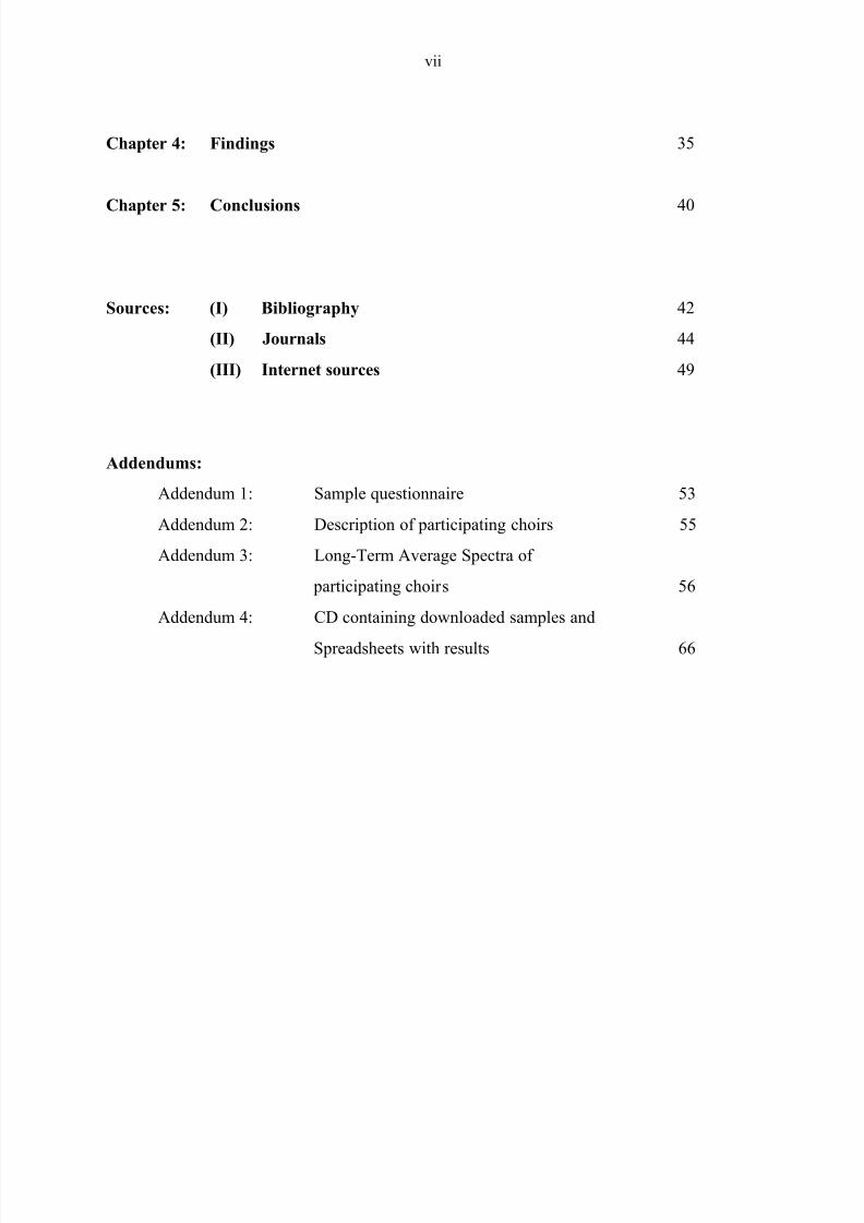
Chapter 4: Findings 35
Chapter 5: Conclusions 40
Sources: (I) Bibliography 42
(II) Journals 44
(III) Internet sources 49
Addendums:
Addendum 1: Sample questionnaire 53
Addendum 2: Description of participating choirs 55
Addendum 3: Long-Term Average Spectra of
participating choirs 56
Addendum 4: CD containing downloaded samples and
Spreadsheets with results 66

8/11/2019 FROM PHYSICS TO MUSIC.pdf
http://slidepdf.com/reader/full/from-physics-to-musicpdf 8/75
viii
L IST OF F IGURES
Page
Figure 1.1 The Sound Wave Created by a Tuning Fork 7
Figure 1.2 How a Vibrating Tuning Fork Causes Air Column Resonance 12
Figure 1.3 Standing Wave Patterns 14
Figure 1.5 The Larynx 16
Figure 1.6 Vocal Folds 17
Figure 1.7 The Mechanism Controlling the Vocal Folds 18Figure 1.8 Jussi Bjoerling Spectral Analysis 26
8/11/2019 FROM PHYSICS TO MUSIC.pdf
http://slidepdf.com/reader/full/from-physics-to-musicpdf 9/75
ix
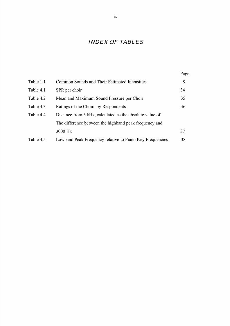
I NDEX OF TABLES
Page
Table 1.1 Common Sounds and Their Estimated Intensities 9
Table 4.1 SPR per choir 34
Table 4.2 Mean and Maximum Sound Pressure per Choir 35
Table 4.3 Ratings of the Choirs by Respondents 36
Table 4.4 Distance from 3 kHz, calculated as the absolute value of
The difference between the highband peak frequency and
3000 Hz 37
Table 4.5 Lowband Peak Frequency relative to Piano Key Frequencies 38
8/11/2019 FROM PHYSICS TO MUSIC.pdf
http://slidepdf.com/reader/full/from-physics-to-musicpdf 10/75
1
CHAPTER 1: BACKGROUND: DEFINING THE SCOPE AND
TERMS OF STUDY
1.1 INTRODUCTION TO THIS STUDY
Although there are many articles and books on formants and overtones produced by soloists
like opera singers and specifically about the so-called singer‟s formant, little research has
been done about the “collective formants” or overtones of a group of singers such as in a
choir. Sundberg notes that:
Most people who use their voices for musical purposes are choir singers. Still, very little
research has been devoted to choir singing, perhaps because it is generally regarded as a
less heroic and spectacular form of voice use than solo singing (Sundberg, 1987:4).
He continues:
Choral singing is probably the most widespread type of singing. Therefore the particular
voice usage under such conditions is an important subject to research. Yet almost all
research on the singing voice concerns operatic singing. ….there are not many facts to
report about choral singing (Sundberg, 1987:134).
Choral directors and voice teachers often strongly disagree about what the effects of choral
singing would be on the vocal development of a singing student. Sundberg (1987:141)
demonstrates that this is an international phenomenon when he writes: “Choral directors and
singing teachers sometimes heatedly discuss whether or not future solo singers should sing in
choirs: is choral singing advantageous for learning solo singing?” It is my experience that at
at least two major universities in South Africa singing students are strongly discouraged from
singing in the university choirs. Informal discussions with voice teachers and vocal students at
those universities show that singing in a choir is regarded by voice teachers as detrimental to
the vocal development of their students. This stands in contrast with students of orchestral
instruments that are not only encouraged by their teachers to play in ensembles and
orchestras, but find it compulsory to do so when studying at tertiary institutions. However,
there exists very little empirical evidence to support arguments on both sides of the vocal
divide. When Sundberg writes “Lively discussions tend to emerge when the base of objective
knowledge is fragile; the less one knows the stronger one feels” , the importance of adding
vocal research focusing in a choral environment becomes clear.
8/11/2019 FROM PHYSICS TO MUSIC.pdf
http://slidepdf.com/reader/full/from-physics-to-musicpdf 11/75
2
When it comes to “good” or “poor” voices, there is distinct lack of tools to deal with the
subject on an unambiguous and scientific level. “Good” or “bad” is most often determined by
the subjective perspective of the listener. This study therefore starts off by trying to define a
“good” choral tone. It then deals with some of the physics underlying sound, including
defining the terminology involved in measuring sound waves, as that knowledge is
fundamental to fully understanding overtones. It then links the knowledge of sound waves
with the sound producing mechanism in the human body. With that background the reader is
now able to understand what is meant by the singing power ratio (SPR) and a long-term
average spectrum analysis (LTAS). The study then analyses the LTAS and SPR for a number
of sound samples of choirs, comparing it to a binary value judgment by a panel, to establish a
possible link between SPR and a “good” choral tone.
1.2 DEFINING A “GOOD” CHORAL TONE
The four main properties of musical sound are generally agreed to be pitch, dynamics, tone
colour (timbre) and meter. Three of these, namely pitch, dynamics and meter, each have an
extensive language capable of describing them very well. We have instruments to measure
and words to describe how “high” or “low” a note is. The musical terminology that describes
how different notes that are grouped together relate to each other, both horizontally (melody)
and vertically (harmony) is well developed. We can scientifically measure the loudness of a
note and we have terminology to give a performer an indication of what dynamic level is to
be expected. Western music notation also makes it easy for a composer to convey detailed
information regarding rhythm and tempo to a performer. There is a solid body of knowledge,
grounded in academia, available to both the performer and the listener to thoroughly quantify,
describe, analyze and/or criticize these aspects of a musical performance. There are also
physical tools available for this process, tools that can be tremendously helpful, but
sometimes also extremely intimidating: seeing an adjudicator at a choral competition picking
up a pitch fork at the end of a performance to check if the choir is still in tune, for example,
can be very unnerving for singers who have just sung their hearts out! We have thus both the
(scientific) language and the necessary tools (pitch fork; correctly tuned instruments;
metronome) to guide both the performer seeking to correctly interpret a piece of music and

8/11/2019 FROM PHYSICS TO MUSIC.pdf
http://slidepdf.com/reader/full/from-physics-to-musicpdf 12/75
3
the adjudicator /examiner that has to decide how “correct” or “good” a particular performance
was in terms of pitch, dynamics and meter.
However, when it comes to tone colour (or “timbre”), we seem to be at a loss when we need
to unambiguously describe what we hear. We understand timbre to be that quality of sound
that distinguishes two instruments from each other at the same pitch and loudness to the
human ear (Handel, 2004:588), or that portion of sound that makes an individual voice
unique, or the sound quality that distinguishes a “good” choral tone from a “poor” one. But
“as early as the twelfth century, the translator Dominicus Gundissalinus noted that there were
no words to describe differences in sound quality; different sounds had no names of their
own, but were described by analogy with other senses” (Fales, 2002:92). McAdams describes
timbre as “the psycho-acoustician's multidimensional waste-basket category for everything
that cannot be labeled pitch or loudness” (McAdams & Bregman, 1979:34). This is further
stressed by Fales when she writes: “We have a peculiar amnesia in regard to timbre, but we‟re
not deaf to timbre: we hear it, we use it – no one has much trouble telling instruments apart –
but we have no language to describe it. With no domain-specific adjectives, timbre must be
described in metaphor or by analogy to other senses, and this is true in many, many languages
of the world” (Fales, 2002:57).
Although musicologists have not yet parameterized timbre as they have done to pitch,
dynamics and meter, this does not mean that a listener has no ability to add a qualitative value
to what he or she is hearing. In his master‟s treatise A critical investigation of the effectiveness
of warm-ups as technical exercises for the improvement of choral tone (Van Zyl, 2006), for
example, Lionel van Zyl does not find it necessary to define a good choral tone, but bases his
study on the assumption that the reader and listener will recognize it when it is heard.
Western music‟s focus on melody and harmony and neglect of timbre in forma lizing the
music system is described as “pitch centrism” by Cornelia Fales when she comments as
follows on recordings of Burundi Whispered Inanga made in 1950:
[...]Merriam‟s recordings of the music betray the subtle bias of what has come to be called “pi tch
centrism” or “timbre deafness”, a perceptual proclivity on the part of western listeners, including
ethnomusicologists, to focus on melody in music where the dominant parameter is timbre. Listeners
from a culture where pitch is governed by law while timbre is governed by taste, where musical
execution is judged correct or incorrect according to variations in pitch, while variations in other
parameters of music are judged pleasing or displeasing – such listeners would be surprised and
perhaps disoriented to find the opposite polarity in evaluations of the Whispered Inanga. A
performance of the Inanga is judged incorrect if the expected timbral effect is imprecisely executed,
8/11/2019 FROM PHYSICS TO MUSIC.pdf
http://slidepdf.com/reader/full/from-physics-to-musicpdf 13/75
4
whereas wide deviations in pitch are considered ornamental, expressive or if unsuccessful, in bad
taste or inappropriate. (Fales, 2002:56).
She continues:
To the general (western) listener, pitch and loudness are variable characteristics of sound, timbre is a
condition; pitch and loudness are things a sound does, timbre is what a sou nd is […] As scholars,indeed as listeners, we have a difficult time describing timbre. […] - it is only by deliberate effort
that we conceptualize it as a distinctly ongoing, dynamic feature of music with the same clarity as
pitch or meter […] We may have difficulty in describing, or even conceptualizing timbre as an
independent musical parameter on the basis of direct examination, but we use it easily to distinguish
or characterize sounds (Fales, 2002:60).
Vurma and Ross (2002:383) discuss the use of metaphoric language by professional singers
and singing instructors in the development of a good vocal tone. They argue that expressions
such as e.g. “supported voice” and “directed to the mask” carry well defined meaning in the
singing environment even though it is often impossible to literally describe or understand the
difference between a “supported” and an “unsupported” voice.
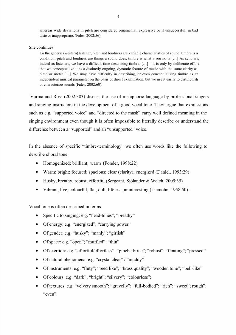
In the absence of specific “timbre-terminology” we often use words like the following to
describe choral tone:
Homogenized; brilliant; warm (Fonder, 1998:22)
Warm; bright; focused; spacious; clear (clarity); energized (Daniel, 1993:29)
Husky, breathy, robust, effortful (Sergeant, Sjölander & Welch, 2005:35)
Vibrant, live, colourful, flat, dull, lifeless, uninteresting (Liemohn, 1958:50).
Vocal tone is often described in terms
Specific to singing: e.g. “head-tones”; “breathy”
Of energy: e.g. “energized”; “carrying power”
Of gender: e.g. “husky”; “manly”; “girlish” Of space: e.g. “open”; “muffled”; “thin”
Of exertion: e.g. “effortful/effortless”; “pinched/free”; “robust”; “floating”; “pressed”
Of natural phenomena: e.g. “crystal clear” / “muddy”
Of instruments: e.g. “fluty”; “reed like”; “brass quality”; “wooden tone”; “bell-like”
Of colours: e.g. “dark”; “bright”; “silvery”; “colourless”;
Of textures: e.g. “velvety smooth”; “gravelly”; “full- bodied”; “rich”; “sweet”; rough”;
“even”.
8/11/2019 FROM PHYSICS TO MUSIC.pdf
http://slidepdf.com/reader/full/from-physics-to-musicpdf 14/75
5
Timbre is also sometimes described in the context of breath control, e.g. “connected” or
“supported”.
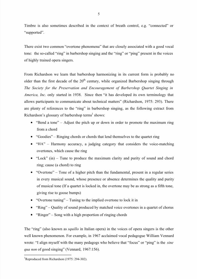
There exist two common “overtone phenomena” that are closely associated with a good vocal
tone: the so-called “ring” in barbershop singing and the “ring” or “ping” present in the voices
of highly trained opera singers.
From Richardson we learn that barbershop harmonizing in its current form is probably no
older than the first decade of the 20 th century, while organized Barbershop singing through
The Society for the Preservation and Encouragement of Barbershop Quartet Singing in
America, Inc. only started in 1938. Since then “it has developed its own terminology that
allows participants to communicate about technical matters” (Richardson, 1975: 293). There
are plenty of references to the “ring” in barbershop singing, as the following extract from
Richardson‟s glossary of barbershop terms1 shows:
“Bend a tone” – Adjust the pitch up or down in order to promote the maximum ring
from a chord
“Goodies” – Ringing chords or chords that lend themselves to the quartet ring
“HA” – Harmony accuracy, a judging category that considers the voice-matching
overtones, which cause the ring
“Lock” (in) – Tune to produce the maximum clarity and purity of sound and chord
ring; cause (a chord) to ring
“Overtone” – Tone of a higher pitch than the fundamental, present in a regular series
in every musical sound, whose presence or absence determines the quality and purity
of musical tone (If a quartet is locked in, the overtone may be as strong as a fifth tone,
giving rise to goose bumps)
“Overtone tuning” – Tuning to the implied overtone to lock it in
“Ring” – Quality of sound produced by matched voice overtones in a quartet of chorus
“Ringer” – Song with a high proportion of ringing chords
The “ring” (also known as squillo in Italian opera) in the voices of opera singers is the other
well known phenomenon. For example, in 1967 acclaimed vocal pedagogue William Vennard
wrote: “I align myself with the many pedagogs who believe that “focus” or “ping” is the sinequa non of good singing” (Vennard, 1967:156).
1Reproduced from Richardson (1975: 294-302).

8/11/2019 FROM PHYSICS TO MUSIC.pdf
http://slidepdf.com/reader/full/from-physics-to-musicpdf 15/75
6
1.3 THE PHYSICS OF SOUND
In order to fully understand concepts such as overtones, the barbershop “ring” and the
singer‟s formant, it is necessary to have a thorough technical understanding of what “sound”
is and how it is produced in the human vocal tract.
1.3.1 Defining Sound
Sound can be defined as a longitudinal, mechanical pressure-wave, transporting energy from
one location to another through an elastic medium (Henderson, 2006a:1, 2006b:1).
A mechanical wave does not have mass and is therefore not an entity like a particle. It
represents the movement of a disturbance through a medium. A very good example of a
mechanical wave is the so-called “Mexican wave” seen at sports events: a portion of the
crowd in the stadium stand up, wave their arms and sit down. They are followed by the people
on e.g. their right (depending on which direction the wave is travelling) and as they in turn sit
down, the people on their right follow. Thus, the “stand up, wave, sit down” action travels
around the stadium. It is obvious that the people performing the action do not travel around
the stadium, only the action. The people in the stadium would represent the medium through
which the wave travels. If they are all sitting quietly, the medium would be said to be in
equilibrium. When someone stands up the equilibrium of the medium is disturbed and it is
this disturbance that moves around the stadium and is called a wave. A mechanical wave
cannot exist if there is no medium through which it can travel. The absence of a medium
explains why sound cannot travel through a vacuum.
Electromagnetic waves differ from mechanical waves in that they require no medium to
propagate. Examples of electromagnetic waves are visible light, infrared waves, microwaves
and radio waves. Other examples of mechanical waves are waves in a pond, sound in the air,
sound under water, the vibrations in a violin string, vibrations in the steering wheel of a motor
car with unbalanced tires and the shock waves of an earth quake.
Sound travels through the air as a pressure-wave. All sound waves are created by a vibrating
object which could be, for example, the vocal chords of a person, the vibrating strings and
soundboard of a guitar or violin or, as mentioned by Harby (1998:2), the vibrating air column
in a trumpet or flute. Vibrations from the source are passed on to the surrounding air particles,
which in turn start to vibrate. As an air particle starts to vibrate, the air-pressure at that point

8/11/2019 FROM PHYSICS TO MUSIC.pdf
http://slidepdf.com/reader/full/from-physics-to-musicpdf 16/75
7
changes slightly. This “change in air - pressure” is passed on to the air particle‟s nearest
neighbours, causing them in turn to be displaced from their equilibrium positions, i.e. to start
vibrating. This particle interaction continues throughout the entire medium, until the energy
transferred to the medium by the source is completely dissipated.
If the direction of the disturbance (e.g. the up-and-down movement of the crowd in the sports
stadium) is perpendicular to the direction in which the waves are moving, it is said to be a
transverse wave. If the direction of the disturbance is parallel to the direction of wave
propagation, it is said to be a longitudinal wave. Sound waves are longitudinal pressure-
waves.
The longitudinal motion of the sound wave creates regions in the air where the air particles
are compressed together (i.e. areas of “high” pressure”) and other regions where the air
particles are spread apart (i.e. areas of “low” pressure”.) These regions are known as
compressions and rarefactions respectively. The compressions and rarefactions are not static,
but move through the medium, leaving the vibrating air particles behind, much like water
waves moving through a pond leave the water molecules behind (Henderson, 2006c:1).
Figure 1.1 depicts a sound wave created by a tuning fork propagating through the air in an
open tube. The compressions and rarefactions are labeled.
Figure 1.1. The Sound Wave Created by a Tuning Fork 2
1.3.2 Measuring sound waves
The wavelength of a sound wave is measured as the distance from one compression to the
next adjacent compression or the distance from one rarefaction to the next adjacent
rarefaction. The frequency of a sound wave is the number of compressions (or rarefactions)
that pass by a specific point in one second. It is measured in Hertz (Hz.). A frequency of 200
2 Reproduced from Henderson (2006c:1)
8/11/2019 FROM PHYSICS TO MUSIC.pdf
http://slidepdf.com/reader/full/from-physics-to-musicpdf 17/75
8
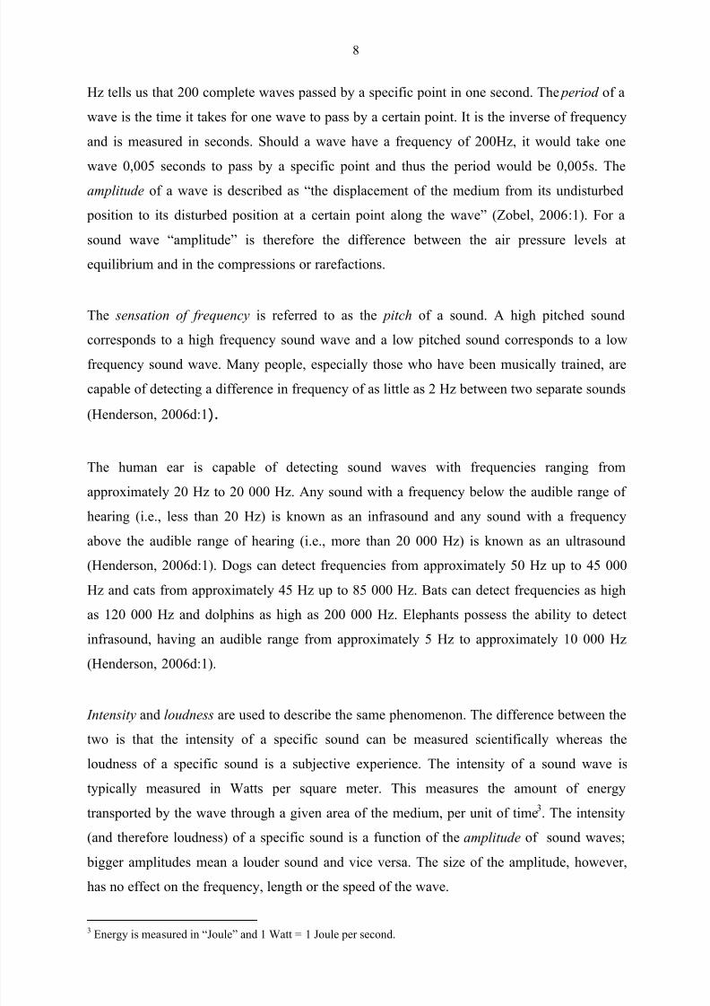
Hz tells us that 200 complete waves passed by a specific point in one second. The period of a
wave is the time it takes for one wave to pass by a certain point. It is the inverse of frequency
and is measured in seconds. Should a wave have a frequency of 200Hz, it would take one
wave 0,005 seconds to pass by a specific point and thus the period would be 0,005s. The
amplitude of a wave is described as “the displacement of the medium from its undisturbed
position to its disturbed position at a certain point along the wave” (Zobel, 2006:1). For a
sound wave “amplitude” is therefore the difference between the air pressure levels at
equilibrium and in the compressions or rarefactions.
The sensation of frequency is referred to as the pitch of a sound. A high pitched sound
corresponds to a high frequency sound wave and a low pitched sound corresponds to a low
frequency sound wave. Many people, especially those who have been musically trained, are
capable of detecting a difference in frequency of as little as 2 Hz between two separate sounds
(Henderson, 2006d:1).
The human ear is capable of detecting sound waves with frequencies ranging from
approximately 20 Hz to 20 000 Hz. Any sound with a frequency below the audible range of
hearing (i.e., less than 20 Hz) is known as an infrasound and any sound with a frequency
above the audible range of hearing (i.e., more than 20 000 Hz) is known as an ultrasound
(Henderson, 2006d:1). Dogs can detect frequencies from approximately 50 Hz up to 45 000
Hz and cats from approximately 45 Hz up to 85 000 Hz. Bats can detect frequencies as high
as 120 000 Hz and dolphins as high as 200 000 Hz. Elephants possess the ability to detect
infrasound, having an audible range from approximately 5 Hz to approximately 10 000 Hz
(Henderson, 2006d:1).
Intensity and loudness are used to describe the same phenomenon. The difference between the
two is that the intensity of a specific sound can be measured scientifically whereas the
loudness of a specific sound is a subjective experience. The intensity of a sound wave is
typically measured in Watts per square meter. This measures the amount of energy
transported by the wave through a given area of the medium, per unit of time3. The intensity
(and therefore loudness) of a specific sound is a function of the amplitude of sound waves;
bigger amplitudes mean a louder sound and vice versa. The size of the amplitude, however,
has no effect on the frequency, length or the speed of the wave.
3 Energy is measured in “Joule” and 1 Watt = 1 Joule per second.
8/11/2019 FROM PHYSICS TO MUSIC.pdf
http://slidepdf.com/reader/full/from-physics-to-musicpdf 18/75
9
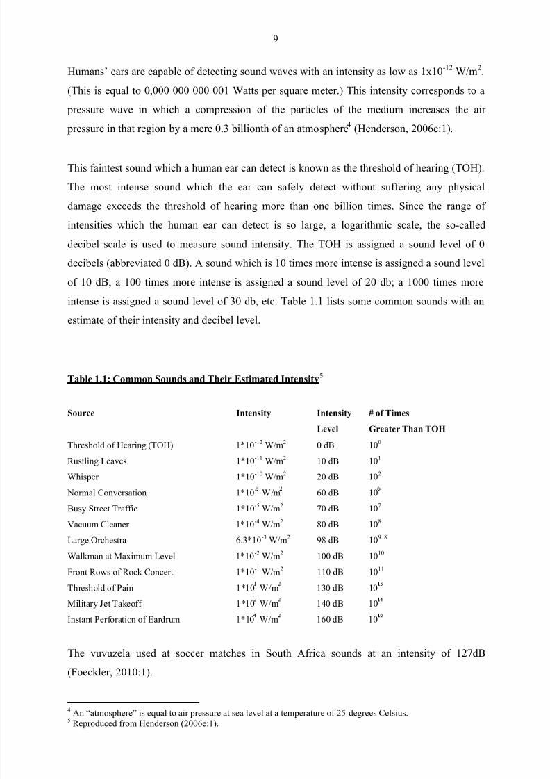
Humans‟ ears are capable of detecting sound waves with an intensity as low as 1x10 -12 W/m2.
(This is equal to 0,000 000 000 001 Watts per square meter.) This intensity corresponds to a
pressure wave in which a compression of the particles of the medium increases the air
pressure in that region by a mere 0.3 billionth of an atmosphere4 (Henderson, 2006e:1).
This faintest sound which a human ear can detect is known as the threshold of hearing (TOH).
The most intense sound which the ear can safely detect without suffering any physical
damage exceeds the threshold of hearing more than one billion times. Since the range of
intensities which the human ear can detect is so large, a logarithmic scale, the so-called
decibel scale is used to measure sound intensity. The TOH is assigned a sound level of 0
decibels (abbreviated 0 dB). A sound which is 10 times more intense is assigned a sound level
of 10 dB; a 100 times more intense is assigned a sound level of 20 db; a 1000 times more
intense is assigned a sound level of 30 db, etc. Table 1.1 lists some common sounds with an
estimate of their intensity and decibel level.
Table 1.1: Common Sounds and Their Estimated Intensity5
Source Intensity Intensity
Level
# of Times
Greater Than TOH
Threshold of Hearing (TOH) 1*10-12
W/m2 0 dB 10
0
Rustling Leaves 1*10-11
W/m2 10 dB 10
1
Whisper 1*10-10
W/m2 20 dB 10
2
Normal Conversation 1*10-
W/m 60 dB 10
Busy Street Traffic 1*10-5
W/m2 70 dB 10
7
Vacuum Cleaner 1*10-4
W/m2 80 dB 10
8
Large Orchestra 6.3*10-3
W/m2 98 dB 10
9. 8
Walkman at Maximum Level 1*10-2
W/m2 100 dB 10
10
Front Rows of Rock Concert 1*10-1
W/m2 110 dB 10
11
Threshold of Pain 1*10 W/m 130 dB 10
Military Jet Takeoff 1*10 W/m 140 dB 10
Instant Perforation of Eardrum 1*10 W/m 160 dB 10
The vuvuzela used at soccer matches in South Africa sounds at an intensity of 127dB
(Foeckler, 2010:1).
4 An “atmosphere” is equal to air pressure at sea level at a temperature of 25 degrees Celsius.
5 Reproduced from Henderson (2006e:1).
8/11/2019 FROM PHYSICS TO MUSIC.pdf
http://slidepdf.com/reader/full/from-physics-to-musicpdf 19/75
10
As previously mentioned, the loudness of a sound is a subjective experience which will vary
from one individual to the next. Factors that can influence experiences of loudness include the
age of the listener and the frequency of the sound. According to Ostrem and Fields the human
ear is not uniformly sensitive to all frequencies. For instance, the ear is most sensitive to
pitches in the 1000-3000Hz range. Lower or higher pitches, even if sung/produced at the same
volume, will sound softer by comparison ( A few Acoustics and Physics Basics, 2009 ).
1.3.3 Properties of mechanical waves relevant to this study
When two objects with mass collide they will either bounce off each other or stick together
after the collision. However, when two waves collide they pass through each other continuing
after the collision as before. At the point of collision they interact with each other and
interference takes place: during the moment of collision the amplitudes of the two waves
combine to form resultant amplitude. Constructive interference takes place when the sum of
the two waves‟ amplitudes is larger than the individual amplitudes, as is the case for sound
waves when two rarefactions or compressions cross each other. Destructive interference takes
place when the sum is smaller than the individual amplitudes, as when a rarefaction from one
sound wave interacts with a compression from another sound wave (Van Zyl, Craül, Meyer &
Oosthuizen, 2002:59). Constructive interference leads to a louder sound and destructive
interference is often the cause of so-called “dead spots” in an auditorium.
The interface of two different media is referred to as a boundary and the behaviour of a wave
at that boundary is described as its boundary behavior. Upon reaching a boundary two things
will happen to a wave travelling through a medium: a) a portion of the wave is reflected and
returns the way it came, b) a portion of the wave is transmitted into the new medium (a
phenomenon known as transmission). The wave which returns to where it came from is
known as the reflected pulse. The amount of energy which becomes reflected (as a wave
travelling in the opposite direction from where it came,) is dependent upon the dissimilarity of
the two mediums. The less similar the two mediums on each side of the boundary are, the
more reflection and the less transmission will occur (Henderson, 2006j:1). A sound wave
traveling through a cylindrical tube will eventually come to the end of the tube. The end of the
tube represents a boundary between the enclosed air in the tube and the expanse of air outside
of the tube. Upon reaching the end of the tube, the sound wave will undergo partial reflection
and partial transmission. This is significant for understanding sounds produced by the human
vocal tract and will be further discussed later in this chapter. If a sound is continuously
generated at one end of a tube, the pulse that is reflected off the other end of the tube will

8/11/2019 FROM PHYSICS TO MUSIC.pdf
http://slidepdf.com/reader/full/from-physics-to-musicpdf 20/75
11
interfere with the sound waves coming towards it and this interference will result in a sound
spectrum unique to the type of instrument.
As mentioned earlier, all sound waves are created as a result of a vibrating object (Van Zyl,
Craül, Meyer & Oosthuizen, 2002:55). Nearly all objects, when hit or struck or plucked or
strummed or somehow disturbed, will vibrate. If you blow over the top of a bottle, for
example, the air inside will vibrate. When each of these objects vibrates, they tend to do so at
a particular frequency or a set of frequencies called the natural frequency of the object .
(Henderson, 2006l:1). If the amplitude of the vibrations is large enough and if the natural
frequency of the object is within the human frequency range, the vibrating object will produce
sound waves which are audible.
There is a vast difference in loudness between the sounds of an acoustic guitar and an
unplugged electric guitar. Although the strings of both instruments vibrate at identical natural
frequencies, the vibrating strings of the acoustic guitar are capable of forcing the wood of the
sound box into vibrating at that same frequency. The sound box in turn forces air particles
inside the box to vibrate at the same frequency as the string. The louder sound is produced
because of the greater surface area of vibrating particles. When a vibrating object forces an
adjoining or interconnected object into vibrational motion it is referred to as forced vibration.
(Henderson, 2009m:1).
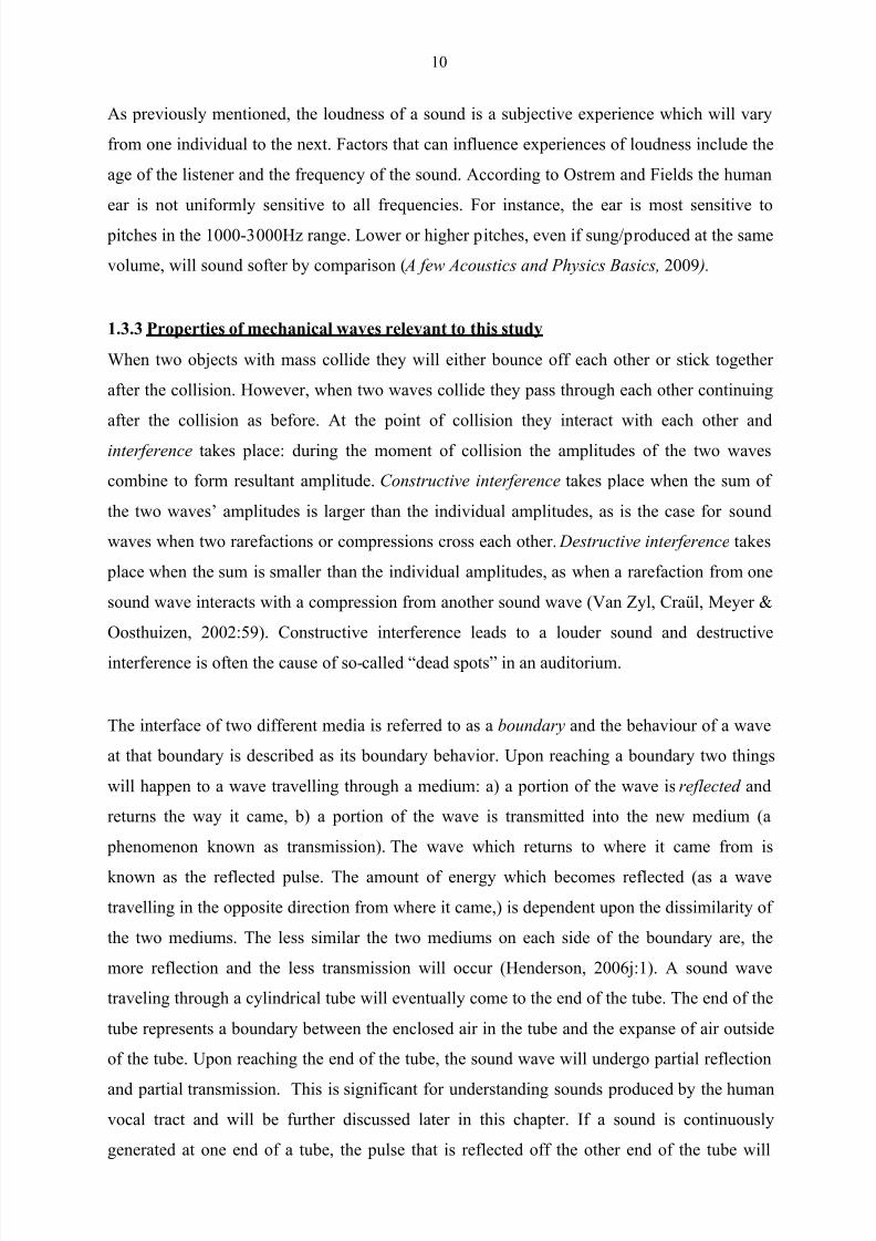
The use of a resonance tube illustrates this phenomenon. It consists of a hollow, cylindrical
tube partially filled with water and connected to a water reservoir as in figure 1.2. A tuning
fork is held at the opening of the resonance tube. The vibrating tines of the tuning fork
(vibrating at their own natural frequency) force the air column in the resonance tube to vibrate
at the same frequency as the tuning fork. The sound of the air column‟s vibration will only be
audible if the natural frequency of the air column matches that of the tuning fork. When this
happens, resonance occurs. The natural frequency of the resonance tube depends on the
diameter of the tube, the smoothness of its surface and the length of the air column in the
tube. In this instance the tube diameter and the surface of the tube remain constant, but the
length of the air column can be altered by raising and lowering the water column in the tube.
Increasing the length of the air column in the tube will decrease the natural frequency of the
air column and vice versa. By raising or lowering the water level of a resonance tube, the
natural frequency of the air in the tube can be matched to the frequency of the vibrating
tuning fork. When this occurs resonance is achieved and a loud sound becomes audible.
8/11/2019 FROM PHYSICS TO MUSIC.pdf
http://slidepdf.com/reader/full/from-physics-to-musicpdf 21/75
12
Figure 1.2: How a Vibrating Tuning Fork Causes Air Column Resonance6
Brass instruments produce sound in a similar manner. Vibrations produced at the mouthpiece
sets the air column in the instrument into vibration. It is the vibration of this air column which
produces the sound that is heard (Harby, 1998: 20). The length of the air column inside the
tube is adjusted by lengthening and shortening the brass tube by either using valves or sliding
the tube. Opening and closing holes in the tube also affects the resonance frequency of the air
column. The vibration of the lips against the mouthpiece produces a range of frequencies.Those frequencies that match the natural frequencies of the air column inside the instrument
are amplified and result in big vibrations and a big sound. (Henderson, 2006p:1)
The quality or timbre of the sound produced by a vibrating object is dependent upon the
natural frequencies of the sound waves produced by the object. The natural frequency (or set
of frequencies) of a wind instrument is a characteristic of its size and shape only and is not
determined by the material from which it is made. This was demonstrated by physicist JohnW. Coltman at a conference on music and human adaptation at Virginia Tech. He played the
same tune twice on a flute without the audience being able to see the instrument. He then
asked the audience to comment on any differences between the two performances. When no
one in the audience could find a difference he revealed that the first time he played the tune, it
was on a simple cherry wood flute and the second time it was on a flute of identical design,
except that it was made of concrete (Harby, 1998: 20).
6 Reproduced from Henderson (2006p:1).

8/11/2019 FROM PHYSICS TO MUSIC.pdf
http://slidepdf.com/reader/full/from-physics-to-musicpdf 22/75
13
When an object is forced into resonance vibrations at one of its natural frequencies, it vibrates
in such a manner that a standing wave pattern is formed within the object. A standing wave
pattern results from the interference of two or more waves moving along the same medium. In
the case of an air column in a hollow tube with a vibrational source at the one end,
interference takes place between incident waves from the source and reflected waves from the
boundary. Nodal and antinodal positions form as a result of the interference. Antinodal
positions are the result of constructive interference (resulting in larger amplitudes at those
points) and nodal positions are the result of destructive interference (resulting in zero
amplitudes at those points). These positions along the medium appear to be standing still
hence the name “standing wave pattern” for this phenomenon. Standing wave patterns are
always characterized by an alternating pattern of nodes and antinodes.
The frequencies at which standing wave patterns are formed are known as harmonic
frequencies. At any frequency other than a harmonic frequency, the interference of reflected
and incident waves results in a wave pattern which is irregular and non-repeating (Henderson,
2006o:1) and sounds to the ear like noise. The natural frequencies of an object are therefore
merely the harmonic frequencies at which standing wave patterns are established within that
object.
A tuning fork produces a “pure tone”, i.e. it sounds at a single frequency, similar to the
electronic production of a single sine wave. However, when sounded at a specific pitch, the
vibrating air column in all wood and brass instruments and in the human vocal tract produce a
set of harmonic frequencies related to each other. Standing wave patterns help us understand
the relationship between the frequencies in the resulting harmonic frequency set.
For any vibrating air column, antinodes (the result of constructive interference) will be
present at any open-end and nodes (the result of destructive interference) at any closed end. If
both ends of the air column are open there will be an antinode at each end with a node in the
middle. Standing wave patterns for the fundamental frequency (or first harmonic) and next
two can therefore be represented as in figure 1.3.
8/11/2019 FROM PHYSICS TO MUSIC.pdf
http://slidepdf.com/reader/full/from-physics-to-musicpdf 23/75
14
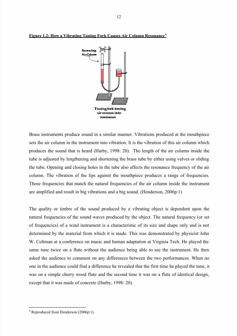
Figure 1.3 Standing Wave Patterns7
If only one of the two lines representing waves in the first harmonic in figure 1.3 is regarded,
it is clear that the length of the air column is equal to half the wavelength of the fundamental
frequency. Adding one more node and antinode to the standing wave pattern will produce the
second harmonic as illustrated in the second harmonic in figure 1.3. In this case the length of
the wave is equal to the length of the air column. Compared to the pattern of the first
harmonic, there are now twice as many waves present in the air columns. The frequency of
the second harmonic is therefore twice the frequency of the first harmonic.
Adding another node and antinode will produce the third harmonic resulting in four antinodes
and three nodes in the air column. In this case there are now one and a half waves present in
the length of the air column. This is equal to three times the numbers of waves present for the
fundamental (or first harmonic.) The frequency of the third harmonic is therefore three times
the frequency of the fundamental. For every node and antinode added to the pattern a
harmonic is added to the frequency set (Henderson, 2006q:1 ).
From the above it follows that all the harmonics in a given frequency set are whole number
multiples of the fundamental frequency (i.e. the first harmonic) and that all the harmonics in
the set are related to each other by whole number ratios.
7 Reproduced from Henderson (2006q:1).
8/11/2019 FROM PHYSICS TO MUSIC.pdf
http://slidepdf.com/reader/full/from-physics-to-musicpdf 24/75
15
The natural frequencies of wood and brass instruments are associated with the standing wave
patterns by which the air column in that object could vibrate that would lead to resonance.
The natural frequencies of a musical instrument are also referred to as the harmonics of the
instrument.
The human vocal tract can be modelled as different combinations of open and closed ended
tubes. Because of the unique construction of the vocal tract, there are numerous natural
frequencies called “formants” built into the instrument. These formants not only determine
which vowels are produced by the singer, but also “much of the personal timbre of the voice”
(Sundberg, 1987:3).
1.4 How sound is produced in the human body
1.4.1 The anatomy of the vocal tract (VT)
The pharynx, or throat, is a hollow tube that extends from the posterior nose to the esophagus
(a tube that connects the pharynx with the stomach) and trachea (windpipe that connects the
pharynx with the lungs). It is divided into the nasopharynx (the area behind the nasal
cavities), the oropharynx (the area around the mouth) and the laryngopharynx (the area above
the trachea and esophagus). The posterior wall of the pharynx consists of the cervical
vertebrae and the side walls are composed of muscle. The anterior wall is first the larynx tube,
next the epiglottis and finally the tongue. There is a cavity between the root of the tongue and
the upper part of the epiglottis. The pharynx is lined with mucous membrane.
The larynx, or voice box as it is more commonly known, is a narrow, short tube, between one
and two centimeters long, that is inserted into the bottom part of the pharynx. The larynx‟s
outer wall of cartilage (the thyroid cartilage) is called the Adam‟s apple. At the top of the
larynx is the glottis, containing the vocal folds (or vocal “chords”). Since air as well as fluids
and food pass through the pharynx, a flap of connective tissue called the epiglottis (“on top
of”- glottis), closes over the larynx during swallowing. In newborn infants, the larynx is
initially further forward and higher relative to its position in the adult body. The larynx
descends as the child grows so that in adult humans, the larynx is found in the anterior neck at
the level of the C3 – C6 vertebrae while in infants at the level of the C2 – C3 vertebrae.

8/11/2019 FROM PHYSICS TO MUSIC.pdf
http://slidepdf.com/reader/full/from-physics-to-musicpdf 25/75
16
Figure 1.4: The Vocal Tract (VT)8
As illustrated in figure 1.5, the main parts of the larynx are the cricothyroid membrane (conus
elasticus), the thyroid-, cricoid- and arytenoid-cartilages and the muscles that control their
movement.
The upper free edge of the conus elasticus is the vocal ligament (or vocal true folds.) Viewed
from the top, the vocal folds form a “V” inside the larynx. Opening and closing of the vocal
folds is controlled by the arytenoid cartilages which separate (“abduct”) or pull together
(“adduct”) the rear end with a rotating movement. The vocal folds can be lengthened and
shortened by controlled movement of the arytenoid cartilage. The longer the vocal folds, the
lower the pitch ranges of the voice. The vocal fold length does not significantly depend on
body length; rather Sundberg reports that it has been found by Sawashima et al. (1983) that
there is a significant correlation between vocal folds length and the circumference of the neck
(Sundberg, 1987:6).
The space between the vocal folds is called the rima glottidis. The ventricular folds are also
known as the “false” vocal chords.
8 Reproduced from Academic Dictionaries and Encyclopedias. Accessed from
http://en.academic.ru/dic.nsf/enwiki/39443 on 8 September 2010.

8/11/2019 FROM PHYSICS TO MUSIC.pdf
http://slidepdf.com/reader/full/from-physics-to-musicpdf 26/75
17
Figure 1.5 The Larynx9
Figure 1.6 Vocal Folds10
9 Reproduced from Larynx. http://www.wesnorman.com/lesson11.htm
10 Reproduced from Gray‟s Anatomy of the Human Body, 1918. Accessed from
http://en.wikipedia.org/wiki/File:Gray956.png on 21 September 2010.

8/11/2019 FROM PHYSICS TO MUSIC.pdf
http://slidepdf.com/reader/full/from-physics-to-musicpdf 27/75
18
Figure 1.7 The Mechanism Controlling the Vocal Folds11
(A) The parts of the larynx involved in breathing and vocalization.
vp – vocal process (lengthening|shortening of vocal folds;
abduction|adduction of vocal folds)
mp – muscular process
ac – arytenoid cartilage
(B) The muscles of the larynx
11 Reproduced from Larynx. http://www.wesnorman.com/lesson11.htm

8/11/2019 FROM PHYSICS TO MUSIC.pdf
http://slidepdf.com/reader/full/from-physics-to-musicpdf 28/75
19
(C) The movements that take place between the arytenoid and cricoid cartilages
AD – adduction
AB – abductionAP – anterior-posterior sliding
ML – medial-lateral sliding
The dots in the arytenoid cartilage are the vertical axis around which
it rotates.
Muscles exert a pull force when they are contracted and therefore shortened. They cannotexert a push force, but are extended either when relaxed or as the result of other muscles
being contracted. The following muscle actions result in vocal cord manipulation:
Transverse arytenoid muscles contract to pull the arytenoid cartilages toward each
other resulting in medial-lateral sliding and adduction (ML)
Contraction of the lateral cricoarytenoid muscles cause the arytenoid cartilages to
rotate which results in adduction. (AD)
Contraction of the posterior cricoarytenoid muscle rotates the arytenoid cartilageslaterally and causes abduction (separation of the vocal chords.) (AB)
Thyroarytenoid muscles pulls the arytenoid cartilages forward (i.e. towards the thyroid
cartilage) which loosens the vocal chords. (AP)
Abduction and adduction enables one to hold your breath and to shift from unvoiced to voiced
sounds and vice versa. In order to produce a voiced sound, the vocal folds must be adducted,
whereas in order to produce an unvoiced sound like whispering or an “s”, the vocal folds must be abducted (“open”).
The combination of the larynx, pharynx and mouth is called the vocal tract and vocal tract
length is defined by Sundberg as the distance from the glottis to the lip opening (Sundberg,
1987:20).

8/11/2019 FROM PHYSICS TO MUSIC.pdf
http://slidepdf.com/reader/full/from-physics-to-musicpdf 29/75
20
1.4.2 The sound producing process
There are three systems involved in the sound producing process: breath, the sound source
and the sound filter. Together they produce a result unique to humans among mammals on our
planet: the ability to create complex language and therefore to communicate complicated
ideas using our voices.
Apart from the fact that an oxygen|carbon dioxide exchange (essential for living), takes place
in the lungs, they also act as an air compressor, capable of providing a constant airflow
through the glottis and vocal tract. The airstream serves two purposes: it acts as resonator in
the vocal tract and it activates and sustains the vocal folds in their function as oscillator.
According to Sundberg the activation process can be explained by the Bernoulli principle
(Sundberg, 1987:12).
Daniel Bernouli was a Swiss mathematician that lived from 1700 to 1782. His most important
work was on the basic properties of fluid dynamics, including fluid flow, pressure, density
and velocity, and his biggest legacy is the Bernoulli principle, which states that as the speed
of a moving fluid increases, the pressure within that fluid decreases. An important application
of this principle is found in the design of airplane wings. The wings are curved on the upper
side and flat underneath. When the aircraft is moving, airflow on the upper side is therefore
faster as the air on that side has a longer distance to travel. The resultant decrease in air
pressure creates a force perpendicular to the movement of the plane, strong enough to lift the
plane off the ground. The speed of fluids and gasses flowing through a confined space like a
pipe (or a pharynx) will increase if the pipe is narrowed. As the speed increases, the pressure
in the constricted portion of the pipe decreases creating a pull force toward the centre of the
pipe.
In order to speak (or sing) the vocal folds are adducted by contracting the lateral
cricoarytenoid muscles. As the vocal folds approach each other, the tube through which air is
flowing is narrowed and the air pressure between the vocal folds drops. This results in a force
pulling the vocal force together. As they touch the airflow is interrupted and air pressure in
the subglottic area builds. This forces the focal folds apart and the air starts flowing again,
repeating the process. By alternately opening and closing, the vibrating vocal folds generate
an acoustic signal composed of variations in the air pressure. The frequency of the tone that is
generated is equal to the “opening and closing” frequency of the vocal folds, in other words,
8/11/2019 FROM PHYSICS TO MUSIC.pdf
http://slidepdf.com/reader/full/from-physics-to-musicpdf 30/75
21
the vibration frequency of the vocal folds. The vocal folds are thus able to act as an oscillator ,
i.e. the source of an acoustic signal. Sundberg states that without the Bernoulli effect voice
sounds would not be possible as nerve signals from the brain, instructing the relevant muscles
to adduct and abduct the vocal folds in order to sustain a vibration, are much too slow to
produce the frequencies needed (Sundberg, 1987:14).
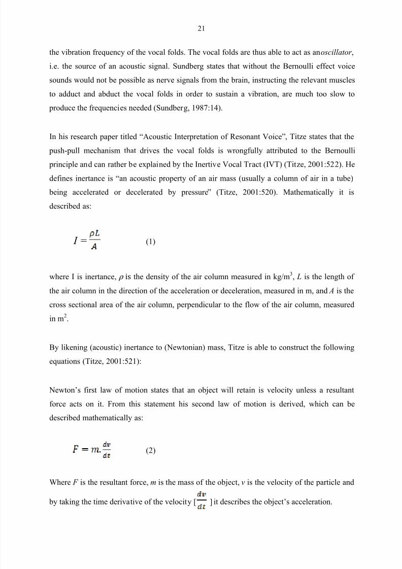
In his research paper titled “Acoustic Interpretation of Resonant Voice”, Titze states that the
push-pull mechanism that drives the vocal folds is wrongfully attributed to the Bernoulli
principle and can rather be explained by the Inertive Vocal Tract (IVT) (Titze, 2001:522). He
defines inertance is “an acoustic property of an air mass (usually a column of air in a tube)
being accelerated or decelerated by pressure” (Titze, 2001:520). Mathematically it is
described as:
I = (1)
where I is inertance, ρ is the density of the air column measured in kg/m 3, L is the length of
the air column in the direction of the acceleration or deceleration, measured in m, and A is the
cross sectional area of the air column, perpendicular to the flow of the air column, measured
in m2.
By likening (acoustic) inertance to (Newtonian) mass, Titze is able to construct the following
equations (Titze, 2001:521):
Newton‟s first law of motion states that an object will retain is velocity unless a resultant
force acts on it. From this statement his second law of motion is derived, which can be
described mathematically as:
(2)
Where F is the resultant force, m is the mass of the object, v is the velocity of the particle and
by taking the time derivative of the velocity [ ] it describes the object‟s acceleration.

8/11/2019 FROM PHYSICS TO MUSIC.pdf
http://slidepdf.com/reader/full/from-physics-to-musicpdf 31/75
22
F can be replaced by P.A (pressure times cross-sectional area in a tube), m can be replaced by
ρ LA (density times length times cross sectional area) and v can be replaced by [ ] (volume
flow per unit area).
Equation 2 now becomes:
P.A = ( .L.A). (3)
Treating A as a constant and substituting equation 1 into it reduces this equation to:
P = [ ] . = I . (4)
Comparing equations 2 and 4 demonstrates the analogy between Newtonian mass and
acoustic inertance. Newton‟s second law states that the acceleration of an object is directly
proportional to the resultant force applied to it for a constant mass. Similarly the acceleration
of the air column particles is directly proportional to the pressure for a constant Inertance. The
air column in the pharynx is accelerated and decelerated by the supra-glottal pressure
described by P in equation 4. It is interesting to note that for frequencies below the first
formant, all the air particles in the entire vocal tract move in the same direction, but not at the
same speed. For frequencies above the first formant, however, movement of the air particles
in the vocal tract is not uniform because sound produced by the vocal chords creates regions
of compression and rarefaction and there are multiple reflected waves creating a number of
standing waves with alternatively high and low regions of particle velocity and pressure. The
vocal folds in the glottis create what is called a phase reversal of the particle velocity (Titze,
2001:521). This simply means that the air particles in the supra-glottal area are accelerated
and decelerated by the opening and closing of the vocal folds. Similar to Sundberg‟s
explanation of the sound source process, the closed vocal folds are driven apart by sub-glottal
pressure; when they open, air-particles accelerate ( is positive), whereas when the vocal
folds start closing because of their elastic recoil, air-particles decelerate ( is negative).
From equation 4 we see that a positive acceleration ( ) results in a higher supra-glottal

8/11/2019 FROM PHYSICS TO MUSIC.pdf
http://slidepdf.com/reader/full/from-physics-to-musicpdf 32/75
23
pressure; this raises the pressure throughout the glottis and helps drive the vocal folds apart.
When the air-particle flow decelerates, it leads to a lower supra-glottal pressure, lowering the
pressure in the entire glottis helping to pull the vocal chords together. This process can be
seen as a non-linear feedback mechanism, where the pressure in the vocal tract, which is
created by the vocal fold movement, drives the vocal fold movement, which in turn feeds
back into the pressure, which in turn feeds back into the vocal fold movement.12 By putting
the supra-glottal pressure in phase with the velocity of the vocal folds, the inertive vocal tract
thus assists vocal fold vibration. Titze states that a highly inertant vocal tract not only makes
it easier for vocal fold vibration to be initiated and sustained, it also “ provides the push-pull
mechanism that is often attributed to the Bernoulli Effect (and wrongfully so)” (Titze,
2001:522).
Sundberg uses the term phonation to refer to the process of generating sound by means of
vocal fold vibrations. He describes the resulting sound as a primary sound and refers to it as
the voice source (Sundberg, 1987:10). If a person was to sing different vowels at the same
loudness and on the same pitch, e.g. A413 (at 440Hz), the voice source would be identical for
all vowels. This implies that in order to produce different vowels, the voice source is changed
or filtered as the sound moves from the glottis to the lips or rather, through the resonator.
During phonation the vocal folds generate an entire spectrum of tones. The lowest tone is
called the fundamental and the rest harmonics or overtones. Together, the fundamental and
overtones are called partials and their frequencies form a harmonic series. Partial number N
will always have a frequency N times that of the lowest partial, i.e. the fundamental. As stated
earlier in this chapter, the frequencies of partials are integer multiples of the fundamental
frequency.
The vocal tract (combination of larynx, pharynx and mouth) has certain inherent resonant
frequencies called formant frequencies that are completely determined by its length and
shape. Partials that match or are close to the vocal tract‟s formant f requencies are
strengthened as the phonated sound travels through it. Different vocal tract shapes therefore
produce different sets of strengthened partials and result both in different vowels uttered by a
12A typical example of non-linear feedback occurs when a microphone is used in front of a speaker: speaking
into the microphone creates sound by the speaker which feeds into the microphone. This quickly leads to a veryloud and often painful noise. 13
The lowest A on the piano is referred to as A0 and the lowest C is referred to as C1, which would make the A
above middle C, A4. Scientific pitch notation. Wikipedia. 2010. Accessed 14 October 2010.
http://en.wikipedia.org/wiki/Scientific_pitch_notation
8/11/2019 FROM PHYSICS TO MUSIC.pdf
http://slidepdf.com/reader/full/from-physics-to-musicpdf 33/75
24
single individual, as well as the perception of individual timbre produced by different singers.
The vocal tract is shaped by the lips, jaw opening, tongue, velum and larynx, which Sundberg
collectively refers to as the articulators (Sundberg, 1987:22). By way of example, he describes
the following actions of the articulators:
The lips can be rounded and spread as we smile. The lower mandible can be moved
upward and downward and also, to some extent, anteriorly and posteriorly. The tongue
can be given a number of different shapes. It can bulge upward and forward, so that it
reaches the hard palate, or upward and backward, so that it approaches the velum, or
downward and backward, so that it constricts the pharynx cavity. The velum can be
raised and lowered. When it is raised, it shuts the connection between the vocal and
nasal tracts; and when it is lowered, the passage between the nose and mouth cavities is
open. Not only can the larynx be raised and lowered, but it can also assume different
shapes, particularly because of the very mobile arytenoid cartilages (Sundberg,
1987:22).
The resonant frequencies (i.e. formants) created by the articulators thus determine the partial
pattern of the filtered sound by changing the shape of the vocal tract. The frequencies of
formants are generally lowered by a narrowing of the lip opening and a lengthening of the
vocal tract (like e.g. protruding lips). Sundberg notes that the first formant frequency
(corresponding to the fundamental of the partial spectrum) responds mainly to changes in the
jaw opening and the second formant frequency to the shape of the tongue. Generally the third
formant frequency is determined by the size of the cavity immediately behind the teeth
created by the tip of the tongue. By moving the articulators the first three formants are easily
manipulated. However, the fourth and fifth formant frequencies are more difficult to
manipulate and are more dependent on vocal tract length than on the specific position of the
articulators. The fourth formant is also very dependent on the shape of the larynx tube
(Sundberg, 1987:23).
Sundberg finally states that vowels are mainly determined by frequencies of the first two
formants. If, for example, the first formant frequency is between 350 and 500Hz and the
second formant frequency between 600 and 800Hz, the vowel will be an /o:/. He also states
that, while vowels are generally defined by the first two formants, voice colour, or timbre, is
mainly determined by the third, fourth and higher formants (Sundberg, 1987:24).
1.4.3 The resonant voice and the singer’s formant
As demonstrated at the start of this chapter, singers use metaphoric language to describe their
experience of acoustic phenomena and singing teachers use it to achieve certain (acoustic)
8/11/2019 FROM PHYSICS TO MUSIC.pdf
http://slidepdf.com/reader/full/from-physics-to-musicpdf 34/75
25
outcomes by their students. A resonant voice is, e.g. often experienced as a sensory perception
of head vibrations, which leads teachers and singers to believe that facial tissues and bone
structures resonate. However the only resonator 14 in those regions that has thus far been
identified resonates at 150Hz. According to Titze it is more likely to be an energy absorber, as
the viscous dissipation within the tissue is very high and acoustic radiation from the tissue
surface is very poor (Titze, 2001:520). Titze further explains that voice production is an
energy conversion process and during phonation aerodynamic energy is converted into
acoustic energy with the sound propagating throughout the entire airway system. He
maintains that if the energy conversion process at the glottis is efficient, vibrations are
distributed all over the head, neck and thorax and especially in the maxillary bony structures
(the hard palate, upper teeth and cheek bones). This results in the false perception amongst
many people that the entire body acts as a resonator when you sing, whereas in fact the human
body contributes nothing to the sound – all the sound produced during singing comes from the
larynx and the air passages, not from “the chest, the back, the belly the buttocks or the legs”
(Titze, 2008:99). Conversely, when the energy conversion process is poor, the vibrations
remain more localised at the glottis with vibrational energy dissipated into the vocal fold
tissues. Vurma and Ross are therefore quite correct when they state that singers “do not
usually employ the term resonance for its scientific meaning, but rather use it loosely to
describe vocal timbre” (Vurma and Ross, 2002:384).
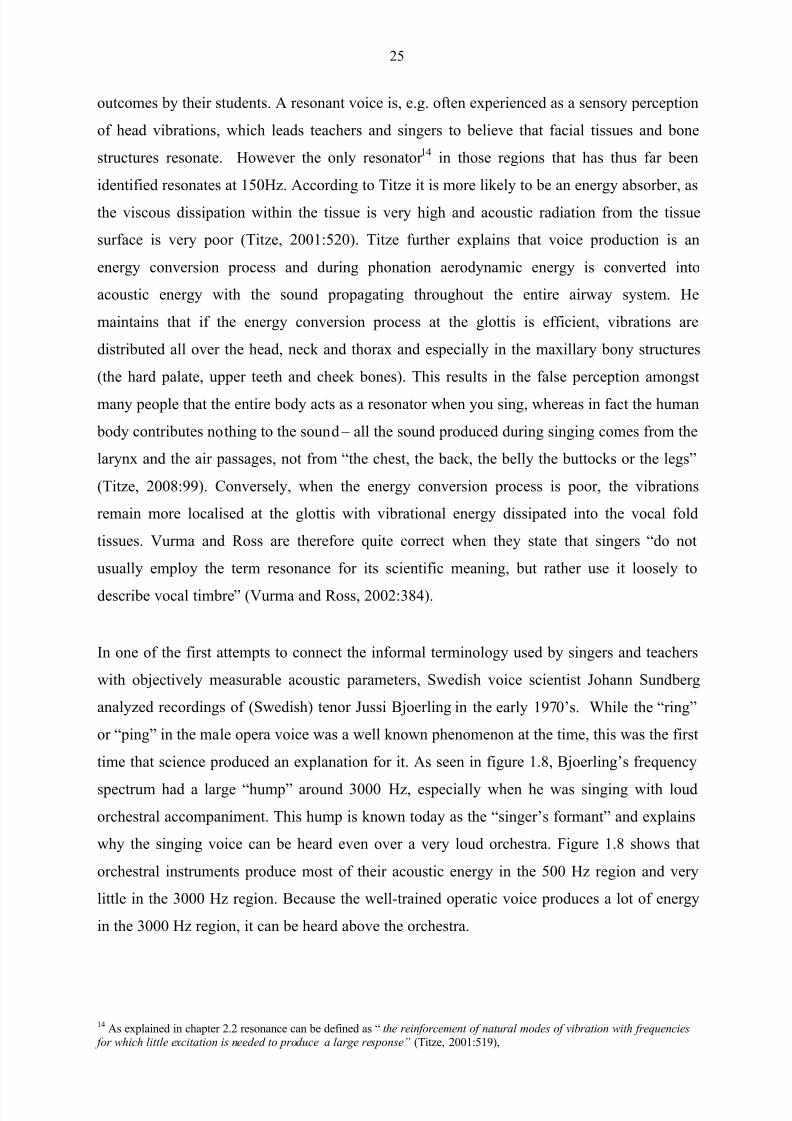
In one of the first attempts to connect the informal terminology used by singers and teachers
with objectively measurable acoustic parameters, Swedish voice scientist Johann Sundberg
analyzed recordings of (Swedish) tenor Jussi Bjoerling in the early 1970‟s. While the “ring”
or “ping” in the male opera voice was a well known phenomenon at the time, this was the first
time that science produced an explanation for it. As seen in figure 1.8, Bjoerling‟s frequency
spectrum had a large “hump” around 3000 Hz, especially when he was singing with loud
orchestral accompaniment. This hump is known today as the “singer‟s formant” and explains
why the singing voice can be heard even over a very loud orchestra. Figure 1.8 shows that
orchestral instruments produce most of their acoustic energy in the 500 Hz region and very
little in the 3000 Hz region. Because the well-trained operatic voice produces a lot of energy
in the 3000 Hz region, it can be heard above the orchestra.
14 As explained in chapter 2.2 resonance can be defined as “ the reinforcement of natural modes of vibration with frequencies for which little excitation is needed to produce a large response” (Titze, 2001:519),
8/11/2019 FROM PHYSICS TO MUSIC.pdf
http://slidepdf.com/reader/full/from-physics-to-musicpdf 35/75
26
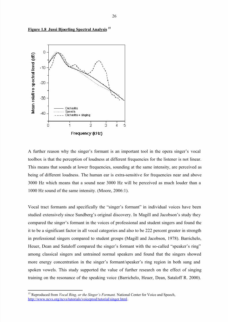
Figure 1.8 Jussi Bjoerling Spectral Analysis15
A further reason why the singer‟s formant is an important tool in the opera singer‟s vocal
toolbox is that the perception of loudness at different frequencies for the listener is not linear.
This means that sounds at lower frequencies, sounding at the same intensity, are perceived as being of different loudness. The human ear is extra-sensitive for frequencies near and above
3000 Hz which means that a sound near 3000 Hz will be perceived as much louder than a
1000 Hz sound of the same intensity. (Moore, 2006:1).
Vocal tract formants and specifically the “singer‟s formant” in individual voices have been
studied extensively since Sundberg‟s original discovery. In Magill and Jacobson‟s study they
compared the singer‟s formant in the voices of professional and student singers and found the
it to be a significant factor in all vocal categories and also to be 222 percent greater in strength
in professional singers compared to student groups (Magill and Jacobson, 1978). Barrichelo,
Heuer, Dean and Sataloff compared the singer‟s formant with the so-called “speaker‟s ring”
among classical singers and untrained normal speakers and found that the singers showed
more energy concentration in the singer‟s formant/speaker‟s ring region in both sung and
spoken vowels. This study supported the value of further research on the effect of singing
training on the resonance of the speaking voice (Barrichelo, Heuer, Dean, Sataloff R. 2000).
15 Reproduced from Vocal Ring, or the Singer’s Formant. National Center for Voice and Speech,
http://www.ncvs.org/ncvs/tutorials/voiceprod/tutorial/singer.html.
8/11/2019 FROM PHYSICS TO MUSIC.pdf
http://slidepdf.com/reader/full/from-physics-to-musicpdf 36/75
27
Miller, Sulter, Schutte and Wolf compared vocal tract formants in singing and nonperiodic
phonation and found that a skilled practitioner can match the first two formants of sung
phonation to nonperiodic phonation with a high degree of accuracy, and that this imitative
process is not primarily based on a pre-conceived posture of the vocal tract. This led them to
conclude that the control mechanism for adjustment of the vocal tract in nonperiodic
phonation is primarily aural (Miller, Sulter, Schutte & Wolf, 1995).
1.5 Summary
This chapter began with the problematisation of existing notions of a “good” choral tone,
highlighting the lack of appropriate theorization of timbre in particular. A brief explanation ofthose physical properties of sound and of the human vocal mechanism which may serve to
provide for such theorization was then given, on which basis a brief overview of the work of
Sundberg and other scholars on the singer‟s formant followed. As highlighted at the start of
this treatise, however, Sundberg has acknowledged that much work in this regard remains to
be done in the case of choral music (Sundberg, 1987: 134). In the following chapter I
therefore attempt to do just that. In selected examples of choral music performances, I attempt
to interrogate the relationship between intuitive value judgments of “good” or “poor” choral
tone, on the one hand, and, on the other hand, the results of the physical analysis of the
spectra of choral formants.
_____________________________________________________________
8/11/2019 FROM PHYSICS TO MUSIC.pdf
http://slidepdf.com/reader/full/from-physics-to-musicpdf 37/75
28
CHAPTER 2: THE SINGING POWER RATI O (SPR) AS AN
OBJECTIVE MEASURE OF CHORAL TONE
2.1 INTRODUCTION
Chapter two highlighted the current lack of appropriate tools to unambiguously distinguish
between a “good ” and a “poor” vocal tone. This does not however, prevent thousands of such
judgments from being made every day. One of the most obvious examples is the judging that
takes place in popular reality TV programs such as “Idols” or “SA‟s got Talent”. Not only
does a panel of supposedly expert judges decide on the quality of a contestant‟s voice; all theviewers feel themselves equally qualified to decide whether a particular singer is “talented” or
not. After all, as the Afrikaans poet, C J Langenhoven anecdotally is claimed to have said: “I
may not be able to lay an egg, but I will know if one is off.”
In their respective studies, Watts, Barnes-Burroughs, Estis and Blanton (2006) as well as
Kenny and Mitchell (2007) describe how binary judgments regarding singing talent (i.e.
“present” vs. “not present”; or “at a required level” vs. “not at a required level”) are routinely
used by, admittedly, professional and experienced adjudicators to judge persons in auditions
for tertiary education programmes and scholarships and in classical music competitions.
However, Kenny makes note of the fact that factors like day, time of day, performer order and
listener fatigue can all affect judgment consistency. He also notes that very little research to
date has linked expert judgments or rankings with acoustic and perceptual factors of vocal
quality (Kenny, 2007:2). In a survey of more than 1000 professional voice teachers that
queried what factors where most important in judging whether an untrained voice expressed
singing talent, Watts et al (2006:83) found that the three most important variables were
intonation, timbre and musicality. As demonstrated in chapter two, ALL the information
about intonation and timbre that reaches the listener or adjudicator, is locked up in the
overtone spectrum. The two studies mentioned in this paragraph are part of an attempt by
voice scientists to unlock the secrets of the overtone spectrum in order to scientifically
quantify and measure timbre.

8/11/2019 FROM PHYSICS TO MUSIC.pdf
http://slidepdf.com/reader/full/from-physics-to-musicpdf 38/75
29
2.2 DEFINING LTAS AND SPR
A long-term average spectrum (LTAS) averages spectral features of the sound signal over
time and thus displays the average sound level in decibels vs. different frequency bands for a
sound sample. It is useful for analysis of voice quality in speech or sung passages of at least
40 seconds and is insensitive to the exact linguistic or musical content (Nordenberg,
Sundberg, 2003:2). It has been used to differentiate between singing styles (pop versus
classical) and different levels of professional achievement (Kenny, Mitchell, 2007:2).
Nordenberg also reports that it has been related to voice quality and gender (Nordenberg,
Sundberg, 2003:93). It clearly demonstrates the presence of the so-called “singer‟s formant”
(a spectral reinforcement around 3kHz) in trained classical and operatic voices.
The information in an LTAS can be reduced to a single meaningful number by computing the
ratio of energies above and below 2 kHz. The Singing Power Ratio (SPR) is calculated by
measuring the ratio of peak intensities between the 2 – 4 kHz and 0 – 2 kHz frequency bands
obtained from an LTAS. The particular frequency bands are chosen because they encompass
the “ring” or “ping” or “singer‟s formant” in the trained opera voice which corresponds to the
resonant quality of the singing voice (Watts et al, 2006: 85). Watts et al (2006) demonstrate
that the SPR can successfully be used as an objective measure of singing voice quality in
untrained talented and non-talented singers. In their methodology they calculate the SPR by
subtracting amplitude of the strongest partial between 2 and 4 kHz from the level of the
strongest partial between 0 and 2 kHz. A lower SPR would indicate greater energy in the
higher harmonics which would influence the perception of voice quality in a positive manner.
The specific research questions that this study aims to answer are the following: 1) Is there a
correlation between the average Singing Power Ratios of a sample of choirs taken from the
public domain and ranked as having a “good” or “poor” sound quality, and the ranking? 2)
Do choirs ranked as “good” on average have a peak in intensity closer to the singer‟s formant
of 3 kHz than those ranked lower? It is hypothesized that on average the SPR of higher
ranked choirs will be lower than that of lower ranked choirs and that higher ranked choirs will
demonstrate an energy peak closer to the singer‟s formant than lower ranked choirs.
_____________________________________________________________
8/11/2019 FROM PHYSICS TO MUSIC.pdf
http://slidepdf.com/reader/full/from-physics-to-musicpdf 39/75
30
CHAPTER 3: THE RESEARCH METHOD AND I TS
APPLICATION
3.1 SOUND SAMPLES
Twenty recordings of “O Magnum Mysterium” by Morten Lauridsen were downloaded from
Youtube using RealPlayer Plus version 14.0.1.609. Samples were converted to uncompressed
.wav audio files and saved. The only criterium used in selecting the samples were availability.
Morten Lauridsen is professor of composition at the University of Southern California
Thornton School of Music. According to his website “O Magnum Mysterium” is one of the
“all-time best selling choral octavos” by publisher Theodore Presser. It was decided to use
this piece because it has been recorded by a large number of choirs and there were at least 20
examples available on Youtube (Morten Lauridson Publications, 2011:1).
Amongst the 20 performances of “O Magnum Mysterium” thus accessed were:
12 University choirs
4 Adult choirs
3 High School choirs
1 Cathedral choir
The sample was also composed of two male voice choirs, two female voice choirs and 16
SATB choirs. Choir sizes varied from vocal ensembles (8 voices) up to 120 voices. A
summary of the choirs, together with links to the respective Youtube sites, are given in
addendum 2.
Recordings were of variable quality, ranging from handheld video recorders with much
audience noise to “ripped” cd‟s. Sound levels and recording devices were uncontrolled and
varied. Recordings of varied quality where deliberately selected since I hypothesized that the
quality of recording level would be reflected in the overtone spectrum and would therefore
influence the decision as to whether a choir had a “good” or “poor” sound.
For the purpose of this study the choirs are not identified.

8/11/2019 FROM PHYSICS TO MUSIC.pdf
http://slidepdf.com/reader/full/from-physics-to-musicpdf 40/75
31
After the recordings were downloaded a sample of each recording was created using
WavePad Audio Editor Version 4.46 to create samples of bars 22 to 34 of the composition in
question. Each .wav sample sound file was created in a PCM Uncompressed format using
settings of 48,000 Hz, 32Bit, Mono. In one case the sample had to be lengthened to bar 35 in
order to get a sample longer than 40 seconds. Sample lengths vary from 40.411 seconds up to
1minute 18 seconds.
3.2 RESEARCH RESPONDENTS
In the different studies involving LTAS and SPR referred to in a previous chapter, experts
were used to determine whether a voice was “good” or “poor”, “acceptable” or
“unacceptable”. These experts made use of years of teaching and performing experience in
making their judgment calls. It remains, however, a subjective view as even an expert‟s
opinion is influenced by his/her concept of an “ideal sound”. From my own experience I
found some of the factors influencing the “ideal choral sound” to be a person‟s cultural
background and choral experience. To paraphrase (the misquoted) Plato, “beauty is (indeed to
some extent) in the eye of the beholder” (Heart, 1997:1). In this study the adjudicating panel
consisted of 50 members of the Pro Cantu Youth Choir of Cape Town, who range in age from
14 to 25 and hail from diverse cultural backgrounds.
The 20 sound samples were played on a mini hi-fi system to the assembled group of 50
respondents. The loudness of each sample was manually adjusted when necessary to ensure
that loudness remained consistent throughout the listening experience. Each member was
provided with a questionnaire and instructed to enter an evaluation of every choir‟s sound or
“voice” relative to the rest of the samples (See addendum 1). Every choir was thus evaluated
on a scale of 1 – 5, where 1 was considered “poor sound, far worse than the rest”, 3 was
considered “average sound, same as the rest” and 5 was considered “fantastic sound, far
better than the rest”. The purpose of the exercise was to divide the samples into two groups
and then to compare the average SPR of the two groups. Having gone through the listening
and ranking exercise on my own beforehand, I realised that if I had used a 3 point scale, i.e.
“average”, “above average” and “below average”, the bulk of the samples would probably
have been rated as average and separating two distinct groups would have been more difficult.
Using a 5 point scale increased the granularity of respondents‟ replies and thus served the
purpose of making the “average” group smaller than with a 3 point scale.

8/11/2019 FROM PHYSICS TO MUSIC.pdf
http://slidepdf.com/reader/full/from-physics-to-musicpdf 41/75
32
Respondents were instructed that giving a choir a mark of 1 did not necessarily mean it was a
bad sound, simply that it was worse than the rest and that the purpose of adjudicating was to
divide the sample of 20 choirs into two groups. Before adjudication started a random selection
of four samples were played to the panel so that they could form an idea as to what the
standard was against which they should measure each choir. They were asked to write down
their first, instinctive reaction. For purposes of possible later referencing, respondents were
asked to provide their names at the top of their questionnaires. Participation was entirely
voluntary.
After adjudication, the average ranking by the respondents for each sample was calculated,
the averages were ranked and the median of the averages were calculated. The samples where
then placed in one of two groups, depending on whether they ranked above the median or
below the median. The groups were labeled “above” and “below”. If the average of a
particular sample was found to be equal to the median, it would be included in the “above”
group.
The listening experience was presented to the 50 respondents on an occasion when they were
meeting together as Pro Cantu members for the first time after recent auditions, and thus there
was amongst them a 21:29 split between experienced choir members and new members. In
order to test if differing choral backgrounds and levels of prior exposure to choral sound
played a role in their decision making, the results in this study are analyzed 1) using the full
sample of choirs and 2) using a sample consisting of only those choirs on which both the
experienced members and the non-experienced members agreed about ranking a choir above
or below the median.
3.3 MEAN AND MAXIMUM SOUND PRESSURE
One of the pitfalls of using LTAS is that it is not uniformly affected by vocal loudness across
the frequency spectrum. In their study “Effect on LTAS of vocal loudness variation” (2003) ,
Norden and Sundberg report that increased vocal loudness causes a larger increase of LTAS
levels at 3 kHz than at 0.5 kHz. This means that when comparing SPR‟s of a choir that is
recorded singing the same song twice, but at different levels of loudness, the louder version
will have stronger partials in the 2 – 4kHz range and therefore exhibit an SPR falsely
signifying a better sound experience than would otherwise be the case. Since the purpose of

8/11/2019 FROM PHYSICS TO MUSIC.pdf
http://slidepdf.com/reader/full/from-physics-to-musicpdf 42/75
33
the study is limited to establishing whether there is a link between a choir‟s SPR and
respondent preference (rather than to determine which choirs have better sounds than the
rest), in this context it is therefore not important why one choir exhibits a lower (or higher)
SPR than another choir; the importance lies rather in merely whether or not it is preferred by
the respondents whilst exhibiting a lower (or higher) SPR. Nevertheless, choirs of whom both
the mean and the maximum sound pressure fell outside 2 standard deviations of the group
mean were excluded from the sample in a secondary investigation in order to examine the
effect of recording loudness on the adjudication respondents‟ preferences.
3.4 ACOUSTIC ANALYSIS
Acoustic analyses of the sample audio files were performed in PRAAT, version 5.2.05
(Boersma and Weenink, 2006). The following analyses were performed on each sound file:
The mean and maximum sound pressure was determined for the audio file (using
parabolic interpolation)
A long-term average spectrum analysis (LTAS) using a 100Hz bandwidth was created
Using the LTAS data, a maximum sound pressure and its corresponding frequency
was determined (using parabolic interpolation) for each sound file in a) the 0 – 2 kHz
range and b) the 2 – 4 kHz range. The corresponding frequency was determined using
linear interpolation.
A graphic representation of each sample‟s LTAS is presented in addendum 3.
The data was then copied into Microsoft Excel for further analysis.
_____________________________________________________________
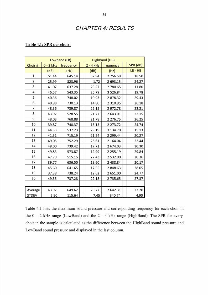
8/11/2019 FROM PHYSICS TO MUSIC.pdf
http://slidepdf.com/reader/full/from-physics-to-musicpdf 43/75
34
CHAPTER 4: RESULTS
Table 4.1: SPR per choir:
Lowband (LB) HighBand (HB)
Choir # 0 - 2 kHz frequency 2 - 4 kHz frequency SPR (dB)
(dB) (Hz) (dB) (Hz) LB - HB
1 51.44 645.14 32.94 2 756.59 18.50
2 25.99 323.96 1.72 2 693.15 24.27
3 41.07 637.28 29.27 2 780.65 11.80
4 46.57 543.35 26.79 3 526.84 19.78
5 40.36 748.02 10.93 2 878.32 29.43
6 40.98 730.13 14.80 2 310.95 26.187 48.36 739.87 26.15 2 972.78 22.21
8 43.92 528.55 21.77 2 643.01 22.15
9 48.03 768.88 21.78 2 276.75 26.25
10 39.87 740.37 15.13 2 273.72 24.74
11 44.33 537.23 29.19 3 134.70 15.13
12 41.51 715.19 21.24 2 299.44 20.27
13 49.05 752.29 26.61 2 164.04 22.44
14 48.00 739.42 17.71 2 674.03 30.30
15 49.83 573.87 19.99 2 255.19 29.84
16 47.79 515.15 27.43 2 532.00 20.36
17 39.77 636.50 19.60 2 438.84 20.17
18 45.60 641.65 17.55 2 848.63 28.05
19 37.38 738.24 12.62 2 651.00 24.77
20 49.55 737.28 22.18 2 735.65 27.37
Average 43.97 649.62 20.77 2 642.31 23.20
STDEV 5.90 115.64 7.45 340.74 4.90
Table 4.1 lists the maximum sound pressure and corresponding frequency for each choir in
the 0 – 2 kHz range (LowBand) and the 2 – 4 kHz range (HighBand). The SPR for every
choir in the sample is calculated as the difference between the HighBand sound pressure and
LowBand sound pressure and displayed in the last column.

8/11/2019 FROM PHYSICS TO MUSIC.pdf
http://slidepdf.com/reader/full/from-physics-to-musicpdf 44/75
35
Table 4.2: Mean and Maximum Sound Pressure per Choir:
Mean Max
Choir # Mean (Pa) Max (Pa) 2 STDEV's
1 -0.0000242 0.57 1 1
2 0.0000103 0.06 1 0
3 -0.0000042 0.43 1 1
4 0.0000021 0.63 1 1
5 0.0001874 0.53 0 1
6 -0.0000130 0.48 1 1
7 -0.0000114 0.88 1 0
8 0.0000113 0.41 1 1
9 -0.0000023 0.74 1 1
10 -0.0000016 0.34 1 1
11 0.0000276 0.55 1 1
12 0.0000004 0.32 1 1
13 -0.0000239 0.75 1 1
14 -0.0000008 0.78 1 0
15 -0.0000615 0.72 0 0
16 0.0000129 0.61 1 1
17 0.0000084 0.26 1 0
18 0.0000010 0.56 1 1
19 0.0000002 0.30 1 0
20 -0.0000102 0.98 1 0
Average 0.0000054 0.54
STDEV 0.0000465 0.23
Upper Limit 0.0000520 0.77
Lower Limit -0.0000411 0.31
The “Mean” and “Max” columns were marked “1” if the particular choir‟s values fell within 2
standard deviations of the group mean and “0” if not. From table 4.2 it follows that choirs 2,
5, 7, 14, 15, 17, 19 and 20 were excluded in a secondary analysis.
After adjudication, the average ranking of each choir was calculated and choirs were placed
into either the “Above” (the median ranking) or “Below” (the median ranking) group. Table
3.3 displays (I) the full sample of choirs, each with its calculated SPR, (II) a sample where
choirs whose mean and maximum pressure fell outside 2 standard deviations from the group
mean were excluded and (III) a sample where the choirs about whom the “experienced” and
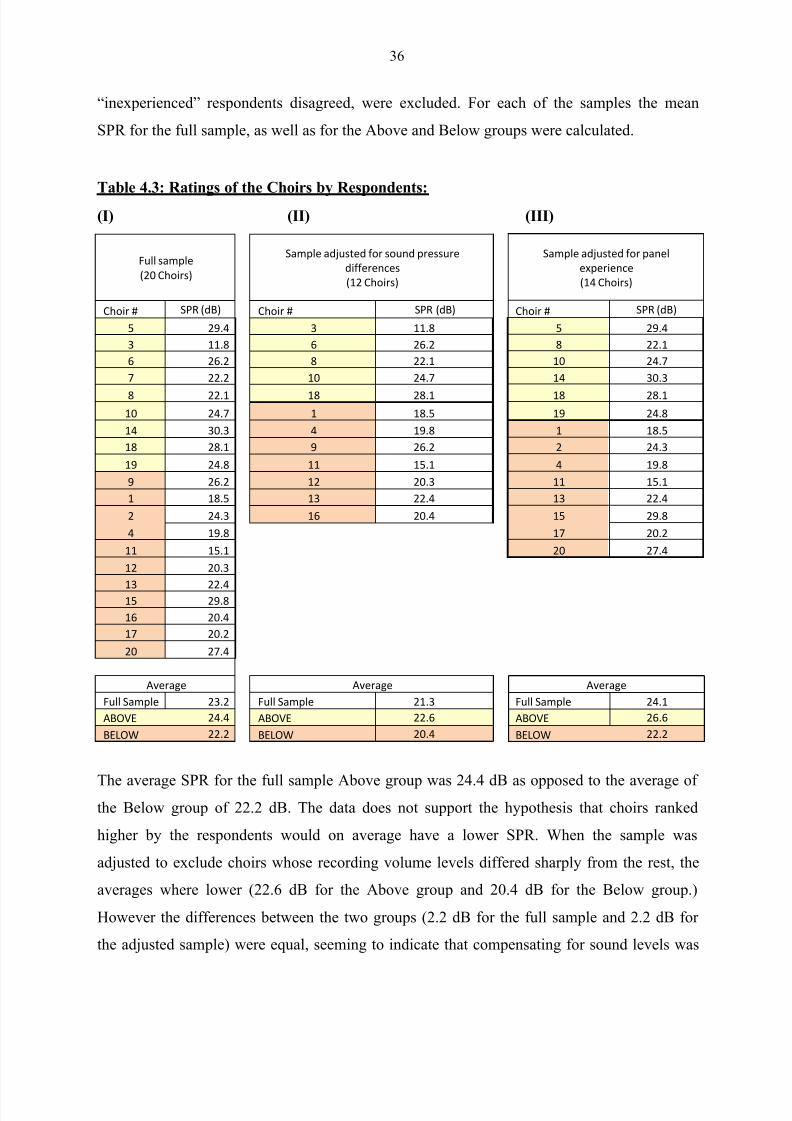
8/11/2019 FROM PHYSICS TO MUSIC.pdf
http://slidepdf.com/reader/full/from-physics-to-musicpdf 45/75
36
“inexperienced” respondents disagreed, were excluded. For each of the samples the mean
SPR for the full sample, as well as for the Above and Below groups were calculated.
Table 4.3: Ratings of the Choirs by Respondents:
(I) (II) (III)
Full sample
(20 Choirs)
Sample adjusted for sound pressure
differences
(12 Choirs)
Sample adjusted for panel
experience
(14 Choirs)
Choir # SPR (dB) Choir # SPR (dB) Choir # SPR (dB)
5 29.4 3 11.8 5 29.4
3 11.8 6 26.2 8 22.1
6 26.2 8 22.1 10 24.7
7 22.2 10 24.7 14 30.3
8 22.1 18 28.1 18 28.1
10 24.7 1 18.5 19 24.8
14 30.3 4 19.8 1 18.5
18 28.1 9 26.2 2 24.3
19 24.8 11 15.1 4 19.8
9 26.2 12 20.3 11 15.1
1 18.5 13 22.4 13 22.4
2 24.3 16 20.4 15 29.8
4 19.8 17 20.2
11 15.1 20 27.4
12 20.3
13 22.415 29.8
16 20.4
17 20.2
20 27.4
Average Average Average
Full Sample 23.2 Full Sample 21.3 Full Sample 24.1
ABOVE 24.4 ABOVE 22.6 ABOVE 26.6
BELOW 22.2 BELOW 20.4 BELOW 22.2
The average SPR for the full sample Above group was 24.4 dB as opposed to the average ofthe Below group of 22.2 dB. The data does not support the hypothesis that choirs ranked
higher by the respondents would on average have a lower SPR. When the sample was
adjusted to exclude choirs whose recording volume levels differed sharply from the rest, the
averages where lower (22.6 dB for the Above group and 20.4 dB for the Below group.)
However the differences between the two groups (2.2 dB for the full sample and 2.2 dB for
the adjusted sample) were equal, seeming to indicate that compensating for sound levels was
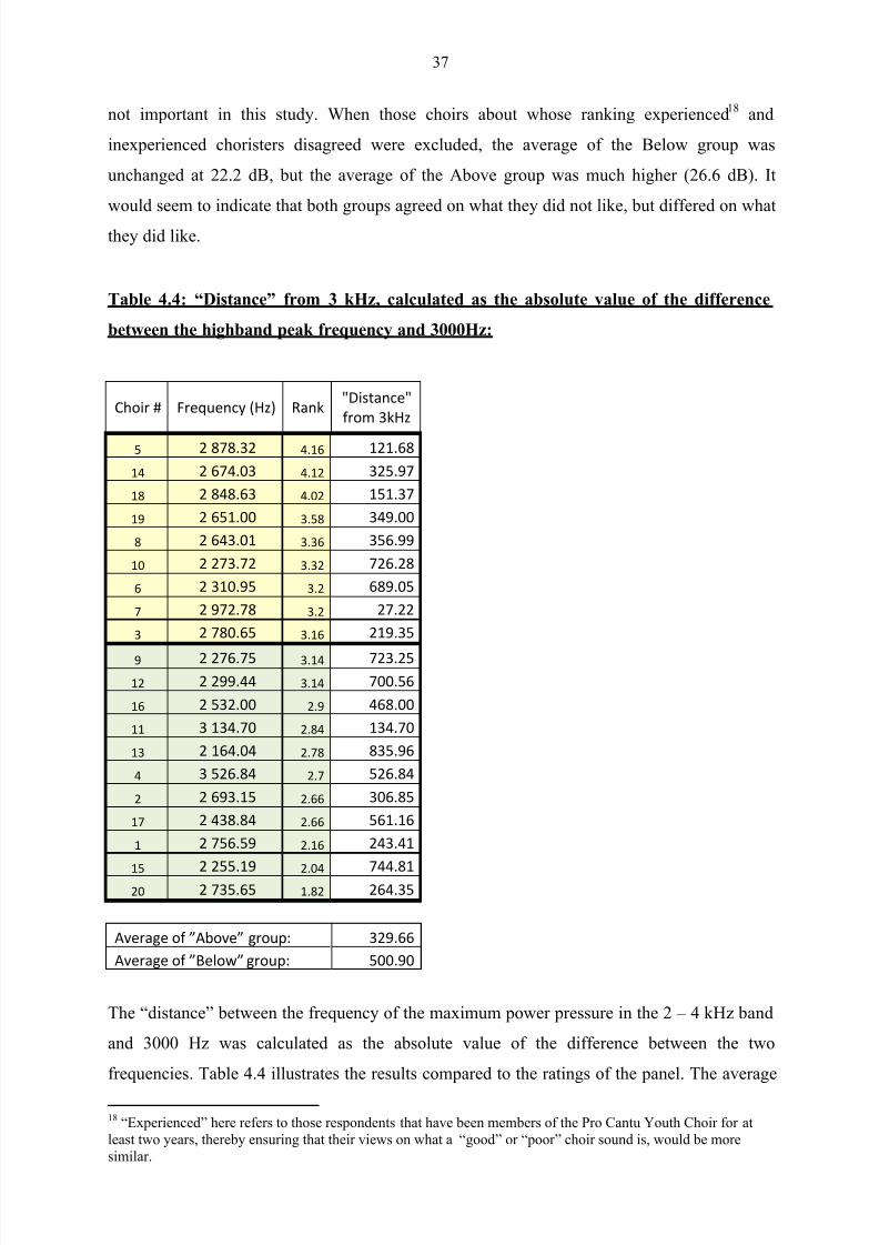
8/11/2019 FROM PHYSICS TO MUSIC.pdf
http://slidepdf.com/reader/full/from-physics-to-musicpdf 46/75
37
not important in this study. When those choirs about whose ranking experienced18 and
inexperienced choristers disagreed were excluded, the average of the Below group was
unchanged at 22.2 dB, but the average of the Above group was much higher (26.6 dB). It
would seem to indicate that both groups agreed on what they did not like, but differed on what
they did like.
Table 4.4: “Distance” from 3 kHz, calculated as the absolute value of the difference
between the highband peak frequency and 3000Hz:
Choir # Frequency (Hz) Rank"Distance"
from 3kHz
5 2 878.32 4.16 121.68
14 2 674.03 4.12 325.97
18 2 848.63 4.02 151.37
19 2 651.00 3.58 349.00
8 2 643.01 3.36 356.99
10 2 273.72 3.32 726.28
6 2 310.95 3.2 689.05
7 2 972.78 3.2 27.22
3 2 780.65 3.16 219.35
9 2 276.75 3.14 723.25
12 2 299.44 3.14 700.56
16 2 532.00 2.9 468.00
11 3 134.70 2.84 134.70
13 2 164.04 2.78 835.96
4 3 526.84 2.7 526.84
2 2 693.15 2.66 306.85
17 2 438.84 2.66 561.16
1 2 756.59 2.16 243.41
15 2 255.19 2.04 744.8120 2 735.65 1.82 264.35
Average of ”Above” group: 329.66
Average of ”Below” group: 500.90
The “distance” between the frequency of the maximum power pressure in the 2 – 4 kHz band
and 3000 Hz was calculated as the absolute value of the difference between the two
frequencies. Table 4.4 illustrates the results compared to the ratings of the panel. The average
18 “Experienced” here refers to those respondents that have been members of the Pro Cantu Youth Choir for at
least two years, thereby ensuring that their views on what a “good” or “ poor ” choir sound is, would be more
similar.

8/11/2019 FROM PHYSICS TO MUSIC.pdf
http://slidepdf.com/reader/full/from-physics-to-musicpdf 47/75
38
“distance” of the Above group from 3 kHz was 329,66 Hz and for the Below group it was
500.90 Hz. This would suggest that the choirs that were preferred by the panelists had energy
peaks in the spectra closer to the singer‟s formant than the rest.
Table 4.5: Lowband Peak Frequency Relative to Piano Key Frequencies:19
Choir #Frequency
(Hz)
Piano
Key
3 637 D#5 | E5
5 748 F#5 | G5
6 730 F5 | F#5
7 740 F#5 | G5
8 529 C5
10 740 F#5
14 739 F#5
18 642 D#5 | E5
19 738 F#5
1 645 D#5 | E5
2 324 E4
4 543 C5 | C#5
9 769 F#5 | G5
11 537 C5 | C#512 715 F5 | F#5
13 752 F#5 | G5
15 574 C5 | C#5
16 515 B4 | C5
17 636 D#5 | E5
20 737 F#5
Average
All 650 D#5 | E5
Above 694 F5
Below 614 D#5
As seen in table 4.5 the average frequency peak in the lower band for all the choirs was 650
Hz, corresponding to a note just below E5 on the piano. The average for the Above group was
694 Hz, (very close to F5 on the piano) and the average for the Below group was 614 Hz (just
below D#5.) This might be an indication of each choir‟s ability to sing the music in question
on pitch and might therefore have played a significant role in whether the respondents
19 Piano key frequencies obtained from Wikipedia, 2010. http://en.wikipedia.org/wiki/Piano_key_frequencies
8/11/2019 FROM PHYSICS TO MUSIC.pdf
http://slidepdf.com/reader/full/from-physics-to-musicpdf 48/75
39
classified such a choir in the Above or Below group. The average frequency peaks of the
LSAT curves relative to a choir‟s ability to perform on pitch is a subject t hat needs to be
examined in a further investigation.
_____________________________________________________________
8/11/2019 FROM PHYSICS TO MUSIC.pdf
http://slidepdf.com/reader/full/from-physics-to-musicpdf 49/75
40
CHAPTER 5: CONCLUSIONS
Although the difference in average SPR between the Above and Below groups is relatively
small, the primary hypothesis of this study is not confirmed by these results. On average the
Singing Power Ratio‟s of the choirs that were preferred by the panel, w ere higher than those
of the non-preferred choirs. This is in contrast with soloists where the SPR‟s of the preferred
voices are on average lower than for non-preferred voices. This suggests that singing power
ratios might be an important variable in analyzing a choir‟s timbre or tone, but it would need
to be interpreted differently. It should be noted however, that the sample size was too small
for statistically conclusive results but it does suggest strongly that examining SPR‟s in a
choral context warrants further investigation.
One of the biggest differences between this study and studies done with solo singers was the
value of the frequency peak in the lower band. In studies with soloists the strongest peak in
the lower band was found to be on the frequency of the fundamental. In this study the
strongest peak was in the fundamental note-range of the soprano voices in the choir. This
suggests that the peak values in the lower band of the LTAS for a choir are stronger than for a
soloist as the energy at this frequency is a combination of the fundamental of the sopranovoices in the choir as well as the first and second overtones of the lower voices. This
phenomenon could explain why the hypothesis was not confirmed by the test results. SPR for
a soloist is calculated as the difference between the strongest frequency band below 2 kHz,
(almost always the fundamental) and the strongest frequency band above 2 kHz. However, the
calculated SPR‟s for this emerged as the difference between the sum of the lower voice
overtones and the upper voice fundamentals on the one hand, and the strongest frequency
band above 2 kHz. This implies that the SPR of soloists and of groups of singers such as in a
choir, are not directly comparable, except if the choir members would all be singing the exact
same note. The results further strongly suggest that singing power ratios for choirs singing in
four or more part harmony will be generally different than the average SPR‟s of the individual
choir members. It would be extremely valuable to conduct further research into this subject in
order to compare the results of a choir‟s SPR with 1) the SPR of each voice group in the choir
and 2) that of the average SPR of each individual member.
The fact that the results of the full sample and the sample that was adjusted to compensate for
recording volume levels were very similar, suggests that meaningful trends could possibly be
8/11/2019 FROM PHYSICS TO MUSIC.pdf
http://slidepdf.com/reader/full/from-physics-to-musicpdf 50/75
41
deducted from samples available in the public domain such as Youtube. However, further
investigation is needed whereby poorer quality public domain samples are compared to the
original recordings before strong conclusions can be drawn.
As stated at the start of this treatise, there exists very little research attempting to scientifically
quantify and analyze timbre for choirs. Analyzing overtone spectra does however provide
important information about the timbre quality of a singer and of a group of singers.
However, the tools that are being developed to analyze solo voices (e.g. SPR‟s) are not likely
to be widely applied in the foreseeable future in real time to adjudicate between good and bad
voices and this is even truer in the case of choral singing. At this stage of development a
possible use of SPR could be to track a specific choir‟s vocal development over a certain time
period, e.g. over two years, by measuring and analyzing it at regular intervals, thereby giving
valuable feedback to the choir‟s vocal coach.
Although the sample size in this study was small, the results point to the need for further in-
depth studies that investigate ways to scientifically quantify timbre in the choir world. This
knowledge will add to our understanding of what constitutes a “good” choral sound and will
contribute to efforts aimed at training choirs and developing wonderful instruments.
_____________________________________________________________

8/11/2019 FROM PHYSICS TO MUSIC.pdf
http://slidepdf.com/reader/full/from-physics-to-musicpdf 51/75
42
SOURCES 20
(I) BIBLIOGRAPHY
Brown, O. 1996. Discover your voice. Clifton Park, NY: Thomson Delmar Learning.
Brewer, M. 2004. Fine-Tune Your Choir . London: Faber Music.
Coffin, B. 1980. Coffin’s Overtones of Bel Canto. Lanham, Maryland: Scarecrow Press.
Ericson, E, Ohlin, G & Spångberg, L. 1974. Choral Conducting. Chapel Hill, N.C.:Hinshaw
Music.
20 Please note that for some electronic journals a Digital Object Identifier (DOI) rather than a web
address is supplied. The following information is extracted from website of The International DOI
Foundation which can be accessed at http://www.doi.org:
The Digital Object Identifier (DOI®) System is for identifying content objects in the
digital environment. DOI® names are assigned to any entity for use on digital networks.
They are used to provide current information, including where they (or information about
them) can be found on the Internet. Information about a digital object may change over
time, including where to find it, but its DOI name will not change.
The DOI System provides a framework for persistent identification, managing intellectual
content, managing metadata, linking customers with content suppliers, facilitating
electronic commerce, and enabling automated management of media. DOI names can be
used for any form of management of any data, whether commercial or non-commercial.
The system is managed by the International DOI Foundation, an open membership
consortium including both commercial and non-commercial partners, and has recently
been accepted for standardisation within ISO. Over 45 million DOI names have been
assigned by DOI System Registration Agencies in the US, Australasia, and Europe.
Using DOI names as identifiers makes managing intellectual property in a networked
environment much easier and more convenient, and allows the construction of automated
services and transactions.
The relevant document is found by typing the DOI number into the search box at http://dx.doi.org/

8/11/2019 FROM PHYSICS TO MUSIC.pdf
http://slidepdf.com/reader/full/from-physics-to-musicpdf 52/75
43
Fenton, W & Johnson, S. 1990. Choral Musicianship: A Director’s Guide to Better Singing
Lebanon, Indiana: Houston Publishing.
Kenny, D & Mitchell, H. 2007. The Vocal audition process: Do you hear what I hear? In
Maimets-Volk, K, Parnutt, R, Marin, M, Ross, J (Eds.) Proceedings of the third Conference
on Interdisciplinary Musicology (CIM07), Talin, Estonia. Accessed from
http://www.composer.in.th/docs/CIM07_Mitchell-Kenny_Open%20throat%20technique.pdf
on 14 December 2010.
Miller, R. 1993. Training Tenor Voices. Belmont, CA: Schirmer Books.
Miller, R. 2008. Securing Baritone, Bass-Baritone and Bass Voices. New York: Oxford
University Press.
Mouton, J. 2001. How to succeed in your Master’s & Doctoral Studies. Pretoria: Van Schaik
Publishers.
Per-Gunnar, A. 2008. Choral intonation. Transl: R Carrol. Stockholm: Germans Musikförlag.
Rogers, E. 1960. Physics for the Enquiring Mind . Princeton: Princeton University Press.
Sawashima, M, Hirose, H, Honda, K, Yoshioka, H, Hibi, S.R, Kawase, N & Yamada M.
1983. Stereoendoscopic measurements of the laryngeal structure. In Vocal fold physiology.
Contemporary research and clinical issues, ed. D.M. Bless and J.H. Abbs, 264-76. San
Diego: College-Hill. In Sundberg, J. 1987. The Science of the Singing Voice. Dekalb, Illinois:
Northern Illinois University Press.
Sundberg, J. 1987. The Science of the Singing Voice. Dekalb, Illinois:Northern Illinois
University Press.
Van Tongeren, M. 2002. Overtone Singing: Physics and Metaphysics of Harmonics in East
and West, Second Edition. Amsterdam: Fusica.

8/11/2019 FROM PHYSICS TO MUSIC.pdf
http://slidepdf.com/reader/full/from-physics-to-musicpdf 53/75
44
Van Zyl, E.J, Craül, V, Meyer, A & Oosthuizen, E. 2002. Second Edition. Ken & Verstaan.
Natuur- en Skeikunde Graad 10. Cambridge: Cambridge University Press : 55-60.
Van Zyl, L. 2006. A critical investigation of the effectiveness of warm-ups as technical
exercises for the improvement of choral tone. Unpublished masters‟ treatise, Nelson Mandela
Metropolitan University, Port Elizabeth.
Vennard, W. 1967. Singing, the mechanism and the Technic, Fifth Edition. New York: Carl
Fischer
(II) JOURNALS
Amir, N. 2004. “Some insight into the acoustics of the didjeridu.” In Applied Acoustics.
65(12): 1181-1196. Accessed on 23 June 2010. DOI: 10.1016/j.apacoust.2004.05.005.
Barrichelo, V, Heuer, R, Dean, C & Sataloff R. 2000. “Comparison of Singer‟s Formant,
Speaker‟s Ring, and LTA Spectrum Among Classical Singers and Untrained Normal
Speakers.” In Journal of Voice 15(3): 344-350.
Beckers, G.J.L, Suthers, R.A. & Ten Cate, C. 2003. “Pure-Tone Birdsong by Resonance
Filtering of Harmonic Overtones”. In Proceedings of the National Academy of Sciences of the
United States of America 100(12):7372-7376. Accessed on 14 December 2009.
http://www.jstor.org/stable/3139484.
Belin, P. 2006. “Voice processing in human and non-human primates”. In Philosophical
Transactions of the Royal Society, London B 2006 361(1476): 2091-2107. Accessed on 14
December 2009. http://rstb.royalsocietypublishing.org/ DOI: 10.1098/rstb.2006.1933.
Bergee, M. & Platt, M. 2003. “Influence of selected variables on solo and small-ensemble
festival ratings.” In Journal of Research in Music Education. 51(4):342-353. In Kenny, D,
Mitchell, H. 2007. The Vocal audition process: Do you hear what I hear? In Maimets-Volk,
K, Parnutt, R, Marin, M, Ross, J (Eds.) Proceedings of the third Conference on
Interdisciplinary Musicology (CIM07), Talin, Estonia.

8/11/2019 FROM PHYSICS TO MUSIC.pdf
http://slidepdf.com/reader/full/from-physics-to-musicpdf 54/75
45
Berndtsson, G. 1996. “The KTH Rule System for Singing Synthesis.” In Computer Music
Journal 20(1): 76-91. Accessed on 14 December 2009. http://www.jstor.org/stable/3681274 .
Daniel, M. 1993. “Balancing Space and Energy in Choral Voices.” In Music Educator’s
Journal. 80(1): 29-31; 51. Accessed on 14 December 2009.
http://www.jstor.org/stable/3398651.
Darwin, C. 2007. “Listening to speech in the presence of other sounds.” In Philosophical
Transactions of the Royal Society, London B 2008 363(1493): 1011-1021. Accessed on 14
December 2009. DOI: 10.1098/rstb.2007.2156.
Diehl, R. 2007. “Acoustic and auditory phonetics: the adaptive design of speech sound
systems.” In Philosophical Transactions of the Royal Society, London B 2008 363: 965-978.
Accessed on 14 December 2009. DOI: 10.1098/rstb.2007.2153.
Ekholm, E. 2000. “The Effect of Singing Mode and Seating Arrangement on Choral Blend
and Overall Choral Sound.” In Journal of Research in Music Education. 48(2): 123-135.
Accessed on 14 December 2009. http://www.jstor.org/stable/3345571.
Fales, C. 2002. “The paradox of timbre”. In Ethnomusicology. 46(1): 56 – 95. Accessed on 14
December 2009. http://www.jstor.org/stable/852808.
Fonder, M. 1998. “Defining and Realizing Your Band‟s Ideal Tone”. In Music Educator’s
Journal. 85(4): 22-25. Accessed on 15 December 2009. http://www.jstor.org/stable/3399141.
Goodwin, A. 1980. “An acoustical study of individual voices in choral blend.” In Journal of
Research in Music Education. 28:(2): 119-128. Accessed on 14 December 2009.
http://www.jstor.org/stable/3344820.
Handel, S & Erickson, M.L. 2004. “Sound Source Identification: The Possible Role of Timbre
Transformations.” In Music Perception: An Interdisciplinary Journal . 21(4):587-610.
Accessed on 19 June 2010. http://www.jstor.org/stable/40285869.
Harby, K. 1998. “Unsound Reasoning.” In Scientific American . March 1998: 20-21.
8/11/2019 FROM PHYSICS TO MUSIC.pdf
http://slidepdf.com/reader/full/from-physics-to-musicpdf 55/75
46
Huston, H.W. 1984. “The Gest of Breath.” In Theatre Journal. 36(2):199-211. Accessed on
24 December 2009. http://www.jstor.org/stable/3206992.
Jacobson, I. 1939. “The Vowel Formant in Vocal Music.” In Music Educators Journal.
26 (3): 21-22. Accessed on 14 December 2009. http://www.jstor.org/stable/3385548 .
Joliveau, E, Smith, J & Wolfe, J. 2004. “Tuning of vocal tract resonance by sopranos.” In
Nature. 427: 116. Accessed on 10 January 2010. http://www.nature.com.
DOI: 10.1038/427116a.
Kinsler, L. "Resonance (acoustics and mechanics)", in AccessScience@McGraw-Hill .
Accessed on 19 June 2010. http://www.accessscience.com, DOI 10.1036/1097-8542.582800.
Levin, T & Edgerton, M. 1999. “The Throat Singers of Tuva.” In Scientific American,
September 1999: 80-87.
Liemohn, E. 1958. “Intonation and Blend in the A Cappella Choir.” In Music Educator’s Journal. 44(6): 50-51. Accessed on 14 December 2009. http://www.jstor.org/stable/3388732.
Lots, I.S. & Stone, L. 2008. “Perception of musical consonance and dissonance: an outcome
of neural synchronisation.” In Journal of the Royal Society Interface. 2008 5: 1429-1434.
Accessed on 14 December 2009. DOI: 10.1098/rsif.2008.0143.
Magill, P & Jacobson, L. 1978, “A Comparison of the Singing Formant in the Voices of
Professional and Student Singers.” In Journal of Research in Music Education 26(4): 456-
469. Accessed on 14 December 2009. http://www.jstor.org/stable/3690716.
Mayer, F.C. 1964. “The Relationship of Blend and Intonation in the Choral Art.” In Music
Educators’ Journal 51(1): 109-110. Accessed on 14 December 2009.
http://www.jstor.org/stable/3390263.
McAdams, S & Bregman, A. 1979. “Hearing Musical Streams”. In Computer Music Journal.
3(4): 26-43; 60. Accessed on 23 December 2009. http://www.jstor.org/stable/4617866.

8/11/2019 FROM PHYSICS TO MUSIC.pdf
http://slidepdf.com/reader/full/from-physics-to-musicpdf 56/75
47
McAdams, S. & Cunible, J. 1992. ”Perception of Timbral Analogies.” In Philosophical
Transactions of the Royal Society, London B 1992 336: 383-389. Accessed on 14 December
2009. DOI: 10.1098/rstb.1992.0072.
McAdams, S. 1999. “Perspectives on the Contribution of Timbre to Musical Structure.” In
Computer Music Journal . 23(3): 85-102. Accessed on 15 December 2009.
http://www.jstor.org/stable/3681242.
McGarry, R.J. 1984. “Equal Temperament, Overtones and the Ear.” In Music Educators’
Journal 70(7): 54-56. Accessed on 14 December 2009. http://www.jstor.org/stable/3400850.
Miller, D.G, Sulter, A.M, Schutte, H.K & Wolf, R. 1997. “Comparison of Vocal Tract
Formants in Singing and Nonperiodic Phonation.” In Journal of Voice 11(1):1-11.
Moore, B. 2002. “Interference effects and phase sensitivity in hearing.” In Philosophical
Transactions of the Royal Society, London A 2002 360: 833-858. Accessed on 14 December
2009. DOI: 10.1098/rsta.2001.0970.
Moore, B. 2007. “Basic auditory processes involved in the analysis of speech sounds.” In
Philosophical Transactions of the Royal Society, London B 2008 363: 947-963. Accessed on
14 December 2009. DOI: 10.1098/rstb.2007.2152.
Musser, G. 1999. “Forming Formants.” In Scientific American, September 1999: 84.
Nordenberg, M & Sundberg, J. 2003. “Effect on LTAS of vocal loudness variation.” In TMH-
QPSR, KTH, (Speech, Music and Hearing. KTH, Stockholm, Sweden). 45:93-100. Accessed
on 14 December 2010.
http://www.speech.kth.se/prod/publications/files/qpsr/2003/2003_45_1_093-100.pdf
Richardson, D. 1975. “The Jargon of Barbershop.” In American Speech 50(3/4): 293-304.
Accessed on 14 December 2009. http://www.jstor.org/stable/3088008.
Rossing, T.D. "Musical acoustics". In AccessScience@McGraw-Hill , Accessed on 19 June
2010. http://www.accessscience.com, DOI 10.1036/1097-8542.440500.

8/11/2019 FROM PHYSICS TO MUSIC.pdf
http://slidepdf.com/reader/full/from-physics-to-musicpdf 57/75
48
Sergeant, D, Sjölander, P & Welch, G. 2005. “Listeners‟ Identification of gender differences
in children‟s singing.” In Research Studies in Music Education 24(1):28-39. Accessed on 21
January 2010. http://www.jstor.org/pss/40319402.
Smith, J. 2007. “Ask the experts”. In Scientific American, September 2007: 124.
Titze, I. 2001. “Acoustic Interpretation of Resonant Voice.” In Journal of Voice 15(4):519-
528.
Titze, I. 2008. “The Human Instrument.” In Scientific American, January 2008: 94-101.
Vurma, A & Ross, J. 2002. “Where Is a Singer‟s Voice if It is Placed „Forward‟?” In Journal
of Voice 16(3):383-391.
Warner, D. 1982. “ Notes from the Timbre Space.” In Perspectives of New Music 21(1/2): 15-
22. Accessed on 15 December 2009. http://www.jstor.org/stable/832866.
Watts, C, Barnes-Burroughs, K, Estis, J & Blanton, D. 2006. “The Singing Power Ratio as an
Objective Measure of Singing Voice Quality in Untrained Talented and Nontalented Singers.”
In Journal of Voice 20(1):82-88.
Weinberger, N. 2004. “Music and the Brain.” In Scientific American, November 2004: 89-95.
Wessel, D. 1979. “Timbre Space as a Musical Control Structure.” In Computer Music
Journal. 3(2): 45-52. Accessed 23 December 2009. http://www.jstor.org/stable/3680283.
(III) INTERNET SOURCES
A few Acoustics and Physics Basics. National Center for Voice and Speech. Accessed on 26
December 2009. http://www.ncvs.org/ncvs/tutorials/voiceprod/tutorial/refresh.html .

8/11/2019 FROM PHYSICS TO MUSIC.pdf
http://slidepdf.com/reader/full/from-physics-to-musicpdf 58/75
49
Arytenoid Cartilage. Accessed on 11 October 2010.
http://en.academic.ru/dic.nsf/enwiki/1178050 .
Boersma, P & Weenink, D. 2006. Praat: Doing phonetics by computer. Accessed 23 October
2009. http://www.fon.hum.uva.nl/praat/.
Daniel Bernoulli. 1998. Accessed on 12 October 2010. http://www-history.mcs.st-
and.ac.uk/Mathematicians/Bernoulli_Daniel.html .
Foeckler, C. 2010. Vuvuzela Unplugged. Accessed on 25 June 2010.
http://www.aolnews.com/the-grid/article/how-loud-are-world-cup-vuvuzela-horns/19515894 .
Heart, S. 1997. Quotes on Beauty. Accessed on 15 December 2010.
http://www.sfheart.com/beauty_quotes.html .
Henderson, T. 2006a. Sound is a mechanical wave. Accessed 26 December 2009.
http://www.physicsclassroom.com/class/sound/u11l1a.cfm .
Henderson, T. 2006b. Sound is a longitudinal wave. Accessed 26 December 2009.
http://www.physicsclassroom.com/class/sound/u11l1b.cfm .
Henderson, T. 2006c. Sound is a pressure wave. Accessed 26 December 2009.
http://www.physicsclassroom.com/class/sound/u11l1c.cfm .
Henderson, T. 2006d. Pitch and frequency. Accessed 26 December 2009.
http://www.physicsclassroom.com/class/sound/u11l2a.cfm .
Henderson, T. 2006e. Intensity and the Decibel Scale. Accessed 26 December 2009.
http://www.physicsclassroom.com/class/sound/u11l2b.cfm .
Henderson, T. 2006f. The Speed of Sound. Accessed 26 December 2009.
http://www.physicsclassroom.com/class/sound/u11l2c.cfm .

8/11/2019 FROM PHYSICS TO MUSIC.pdf
http://slidepdf.com/reader/full/from-physics-to-musicpdf 59/75
50
Henderson, T. 2006g. The Human Ear. Accessed 26 December 2009.
http://www.physicsclassroom.com/class/sound/u11l2d.cfm .
Henderson, T. 2006h. Interference and Beats. Accessed 26 December 2009.
http://www.physicsclassroom.com/class/sound/u11l3a.cfm .
Henderson, T. 2006i. The Doppler Effect and Shock Waves. Accessed 26 December 2009.
http://www.physicsclassroom.com/class/sound/u11l3b.cfm .
Henderson, T. 2006j. Boundary Behaviour. Accessed 26 December 2009.
http://www.physicsclassroom.com/class/sound/u11l3c.cfm .
Henderson, T. 2006k. Reflection, Refraction and Diffraction. Accessed 26 December 2009.
http://www.physicsclassroom.com/class/sound/u11l3d.cfm .
Henderson, T. 2006l. Natural Frequency. Accessed 26 December 2009.
http://www.physicsclassroom.com/class/sound/u11l4a.cfm .
Henderson, T. 2006m. Forced Vibration. Accessed 26 December 2009.
http://www.physicsclassroom.com/class/sound/u11l4b.cfm .
Henderson, T. 2006n. Standing Wave Patterns. Accessed 26 December 2009.
http://www.physicsclassroom.com/class/sound/u11l4c.cfm .
Henderson, T. 2006o. Fundamental Frequency and Harmonics. Accessed 26 December 2009.
http://www.physicsclassroom.com/class/sound/u11l4d.cfm .
Henderson, T. 2006p. Resonance. Accessed 26 December 2009.
http://www.physicsclassroom.com/class/sound/u11l5a.cfm .
Henderson, T. 2006q. Open-End Air Columns. Accessed 26 December 2009.
http://www.physicsclassroom.com/class/sound/u11l5c.cfm .

8/11/2019 FROM PHYSICS TO MUSIC.pdf
http://slidepdf.com/reader/full/from-physics-to-musicpdf 60/75
51
Leeds, J. 2009. The Power of Sound. Accessed 23 December 2009.
http://appliedmusic.com/psycho.html .
Marquis, G. 2010. Lab 1 Introduction. Accessed 13 June 2010.
http://sharepoint.emcc.edu/faculty/gmarquis/PHY124.htm .
MedicineNet.com. Accessed 5 September 2010. http://www.medterms.com.
Mitchell, M. 2003. Animated Demonstration of Ber noulli’s Principle. Accessed 12 October
2010. http://home.earthlink.net/~mmc1919/venturi.html .
Moore, G. 2006. More on Perception of Loudness. Lecture notes for course: Physics 224 at
McGill University, Montreal, Canada. Accessed on 22 December 2010.
http://www.physics.mcgill.ca/~guymoore/ph224/notes/lecture13.pdf .
Mortin Lauridsen Publications. Accessed on 6 January 2011.
http://homepage.mac.com/kennesten/lauridsen/index2.html
Norman, W. 1999a. Larynx. Accessed 11 October 2010.
http://www.wesnorman.com/lesson11.htm.
Norman, W. 1999b. The Anatomy Lesson. Accessed 11 October 2010.
http://www.wesnorman.com/ .
O‟Connor, K. 2009. Vibrato: What it is and how to develop it . Accessed 7 July 2009.
http://www.singwise.com/cgi-bin/main.pl?section=articles&doc=Vibrato&page=1 .
Piano Key Frequencies. 2010. Wikipedia. Accessed on 15 December 2010.
http://en.wikipedia.org/wiki/Piano_key_frequencies .
Pharynx. Academic Dictionaries and encyclopedias. Accessed on 6 September 2010.
http://en.academic.ru/dic.nsf/enwiki/39443 .
8/11/2019 FROM PHYSICS TO MUSIC.pdf
http://slidepdf.com/reader/full/from-physics-to-musicpdf 61/75
52
Russell, D. 2001. Longitudinal and Transverse Wave Motion. Accessed 28 December 2009.
http://paws.kettering.edu/~drussell/Demos/waves/wavemotion.html .
Scientific Pitch Notation. Wikipedia. 2010. Accessed 14 October 2010.
http://en.wikipedia.org/wiki/Scientific_pitch_notation .
Timbre. Statemaster Encyclopedia. Accessed 23 December 2009.
http://www.statemaster.com/encyclopedia/Timbre .
Vocal Ring, or the Singer’s Formant. National Center for Voice and Speech. Accessed on 26
December 2009. http://www.ncvs.org/ncvs/tutorials/voiceprod/tutorial/singer.html .
Wood, S. 2005. Praat for beginners. Accessed 9 February 2007.
http://person2.sol.lu.se/SidneyWood/praate/whatform.html .
Zobel, E. 2006. Parts of a Wave. Accessed 28 December 2009.
http://zonalandeducation.com/mstm/physics/waves/partsOfAWave/waveParts.htm .
8/11/2019 FROM PHYSICS TO MUSIC.pdf
http://slidepdf.com/reader/full/from-physics-to-musicpdf 62/75
53
ADDENDUMS
ADDENDUM 1: QUESTIONAIRE
Name:
This questionnaire forms part of an investigation to establish the link between overtones and
the perceived quality of a choir‟s sound.
In watching reality television programs like “Idols” and “SA‟s got Talent” viewers and judges
are constantly deciding whether a participant has a “good” voice or not. You are requested to
judge the quality of each choir‟s “voice” when listening to the clips that will be played to you.
You will hear ten extracts from songs taken from YouTube. Please rate every clip only on the
quality of the choir‟s sound. Try not to be influenced by whether you like or dislike the song
and by your judgment about the performer‟s interpretation of the song. Also try to not let the
technical quality of the recording influence your decision. The clips will be played in two
rounds. During the first round, do nothing, simply listen. When they are played the second
time, please rate each clip on a scale of 1 – 5 where
1 – Poor sound; far worse than the rest
2 – Not-so-good sound; i.e. not quite on par with the rest
3 – Average sound; same as the rest
4 – Good sound; better than rest
5 - Fantastic sound far better than the rest
Please note that “average” might still be good! If all the choirs are good and they sound the
same, then they should all be marked “average”. The purpose of this exercise is to rank the
choirs, not to establish an absolute value for “good” or “poor”.
Choir 1 1 2 3 4 5
Choir 2 1 2 3 4 5
Choir 3 1 2 3 4 5
Choir 4 1 2 3 4 5
Choir 5 1 2 3 4 5
Choir 6 1 2 3 4 5
Choir 7 1 2 3 4 5

8/11/2019 FROM PHYSICS TO MUSIC.pdf
http://slidepdf.com/reader/full/from-physics-to-musicpdf 63/75
54
Choir 8 1 2 3 4 5
Choir 9 1 2 3 4 5
Choir 10 1 2 3 4 5
Choir 11 1 2 3 4 5
Choir 12 1 2 3 4 5
Choir 13 1 2 3 4 5
Choir 14 1 2 3 4 5
Choir 15 1 2 3 4 5
Choir 16 1 2 3 4 5
Choir 17 1 2 3 4 5
Choir 18 1 2 3 4 5
Choir 19 1 2 3 4 5
Choir 20 1 2 3 4 5
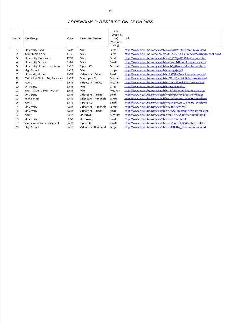
8/11/2019 FROM PHYSICS TO MUSIC.pdf
http://slidepdf.com/reader/full/from-physics-to-musicpdf 64/75
55
ADDENDUM 2: DESCRIPTION OF CHOIRS
Choir # Age Group Voice Recording Device
Size
(Small: <
20 )
(Medium:
< 40)
Link
1 University Choir SATB Mics Large http://www.youtube.com/watch?v=wqalXYh_A0I&feature=related
2 Adult Male Voice TTBB Mics Large http://www.youtube.com/comment_servlet?all_comments=1&v=ki2nheCrwEA
3 University Male Voice TTBB Mics Small http://www.youtube.com/watch?v=X_jP22jwG34&feature=related
4 University Female SSAA Mics Small http://www.youtube.com/watch?v=KVAnRGFsiws&feature=related
5 University alumni - Late teen SATB Ripped CD Medium http://www.youtube.com/watch?v=HkSgUw4lvuc&feature=related
6 High School SATB Mics Large http://www.youtube.com/watch?v=KspgKjAgYfI
7 University alumni SATB Videocam | Tripod Small http://www.youtube.com/watch?v=1J0O8wTzvIc&feature=related
8 Cathedral Choir | Boy Sopranos SATB Mics | prof TV Medium http://www.youtube.com/watch?v=Q7ch7uottHU&feature=related
9 Adult SATB Videocam | Tripod Medium http://www.youtube.com/watch?v=u09AnfsFyik&feature=related
10 University SATB Mics Large http://www.youtube.com/watch?v=GqCtbR8PktU
11 Youth Choir (university age) SATB Mics Medium http://www.youtube.com/watch?v=j2YuHS-vVn4&feature=related
12 University SATB Videocam | Tripod Small http://www.youtube.com/watch?v=cHOtfLvrjI8&feature=related
13 High School SATB Videocam | Handheld Large http://www.youtube.com/watch?v=Buo6tyQqBWI&feature=related
14 Adult SATB Ripped CD Small http://www.youtube.com/watch?v=Buo6tyQqBWI&feature=related
15 University SATB Videocam | Handheld Large http://www.youtube.com/watch?v=7pnA2UzKAv0
16 University SATB Videocam | Tripod Small http://www.youtube.com/watch?v=EvvARM0dmq8&feature=related
17 Adult SATB Unknown Medium http://www.youtube.com/watch?v=zIEEeVZVYjo&feature=related
18 University SSAA Unknown Small http://www.youtube.com/watch?v=0rPK6nHReG4
19 Young Adult (university age) SATB Ripped CD Small http://www.youtube.com/watch?v=nn5ken3RJBo&feature=related
20 High School SATB Videocam |Handheld Large http://www.youtube.com/watch?v=58cfORxy_Rc&feature=related
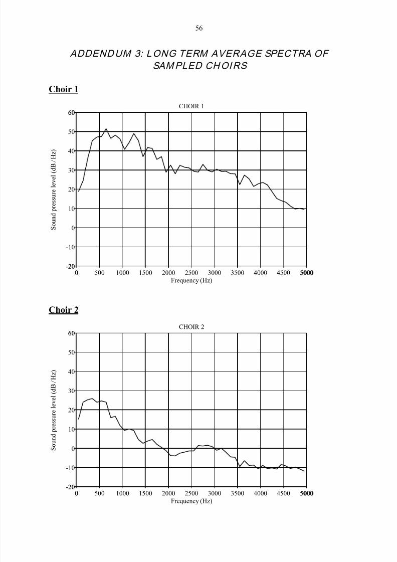
8/11/2019 FROM PHYSICS TO MUSIC.pdf
http://slidepdf.com/reader/full/from-physics-to-musicpdf 65/75
56
ADDENDUM 3: LONG TERM AVERAGE SPECTRA OF
SAMPLED CHOIRS
Choir 1
Frequency (Hz)
0 5000
S o u n d p r e s s u
r e l e v e l ( d B / H z )
-20
60
-20
-10
0
10
20
30
40
50
60
0 500 1000 1500 2000 2500 3000 3500 4000 4500 5000
CHOIR 1
Choir 2
Frequency (Hz)0 5000
S o u n d p r e s s u r e l e v e l (
d B / H z )
-20
60
-20
-10
0
10
20
30
40
50
60
0 500 1000 1500 2000 2500 3000 3500 4000 4500 5000
CHOIR 2

8/11/2019 FROM PHYSICS TO MUSIC.pdf
http://slidepdf.com/reader/full/from-physics-to-musicpdf 66/75
57
Choir 3
Frequency (Hz)
0 5000
S o u n d p r e s s u r e l e v e l ( d B / H z )
-20
60CHOIR 3
0 500 1000 1500 2000 2500 3000 3500 4000 4500 5000-20
-10
0
10
20
30
40
50
60
Choir 4
Frequency (Hz)
0 5000
S o u n d p r e s s u r e l e v e l ( d B / H z )
-20
60
-20
-10
0
10
20
30
40
50
60
0 500 1000 1500 2000 2500 3000 3500 4000 4500 5000
CHOIR 4

8/11/2019 FROM PHYSICS TO MUSIC.pdf
http://slidepdf.com/reader/full/from-physics-to-musicpdf 67/75
58
Choir 6
Frequency (Hz)
0 5000
S o
u n d p r e s s u r e l e v e l ( d B / H z )
-20
60
0 500 1000 1500 2000 2500 3000 3500 4000 4500 5000-20
-10
0
10
20
30
40
50
60CHOIR 6
Choir 7
Frequency (Hz)
0 5000
S o u n d p r e s s
u r e l e v e l ( d B / H z )
-20
60
-20
-10
0
10
20
30
40
50
60
0 500 1000 1500 2000 2500 3000 3500 4000 4500 5000
CHOIR 7
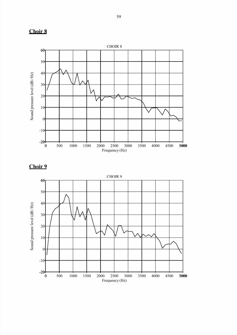
8/11/2019 FROM PHYSICS TO MUSIC.pdf
http://slidepdf.com/reader/full/from-physics-to-musicpdf 68/75
59
Choir 8
Frequency (Hz)
0 5000
S o
u n d p r e s s u r e l e v e l ( d B / H z )
-20
60CHOIR 8
-20
-10
0
10
20
30
40
50
60
0 500 1000 1500 2000 2500 3000 3500 4000 4500 5000
Choir 9
Frequency (Hz)
0 5000
S o u n d p r e s s u r e l e v e l ( d B / H z )
-20
60CHOIR 9
-20
-10
0
10
20
30
40
50
60
0 500 1000 1500 2000 2500 3000 3500 4000 4500 5000
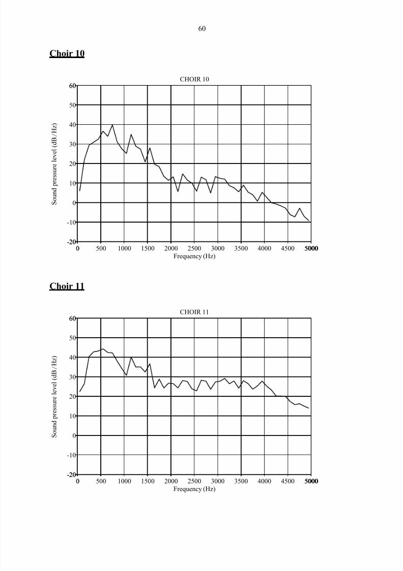
8/11/2019 FROM PHYSICS TO MUSIC.pdf
http://slidepdf.com/reader/full/from-physics-to-musicpdf 69/75
60
Choir 10
Frequency (Hz)
0 5000
S o
u n d p r e s s u r e l e v e l ( d B / H z )
-20
60
0 500 1000 1500 2000 2500 3000 3500 4000 4500 5000-20
-10
0
10
20
30
40
50
60CHOIR 10
Choir 11
Frequency (Hz)
0 5000
S o u n d p r e s s u r e l e v e l ( d B / H z )
-20
60
0 500 1000 1500 2000 2500 3000 3500 4000 4500 5000-20
-10
0
10
20
30
40
50
60CHOIR 11
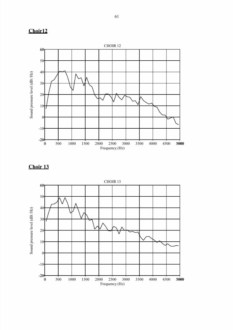
8/11/2019 FROM PHYSICS TO MUSIC.pdf
http://slidepdf.com/reader/full/from-physics-to-musicpdf 70/75
61
Choir12
Frequency (Hz)
0 5000
S o
u n d p r e s s u r e l e v e l ( d B / H z )
-20
60
0 500 1000 1500 2000 2500 3000 3500 4000 4500 5000-20
-10
0
10
20
30
40
50
60CHOIR 12
Choir 13
Frequency (Hz)
0 5000
S o u n d p r e s s u r e
l e v e l ( d B / H z )
-20
60
-20
-10
0
10
20
30
40
50
60
0 500 1000 1500 2000 2500 3000 3500 4000 4500 5000
CHOIR 13
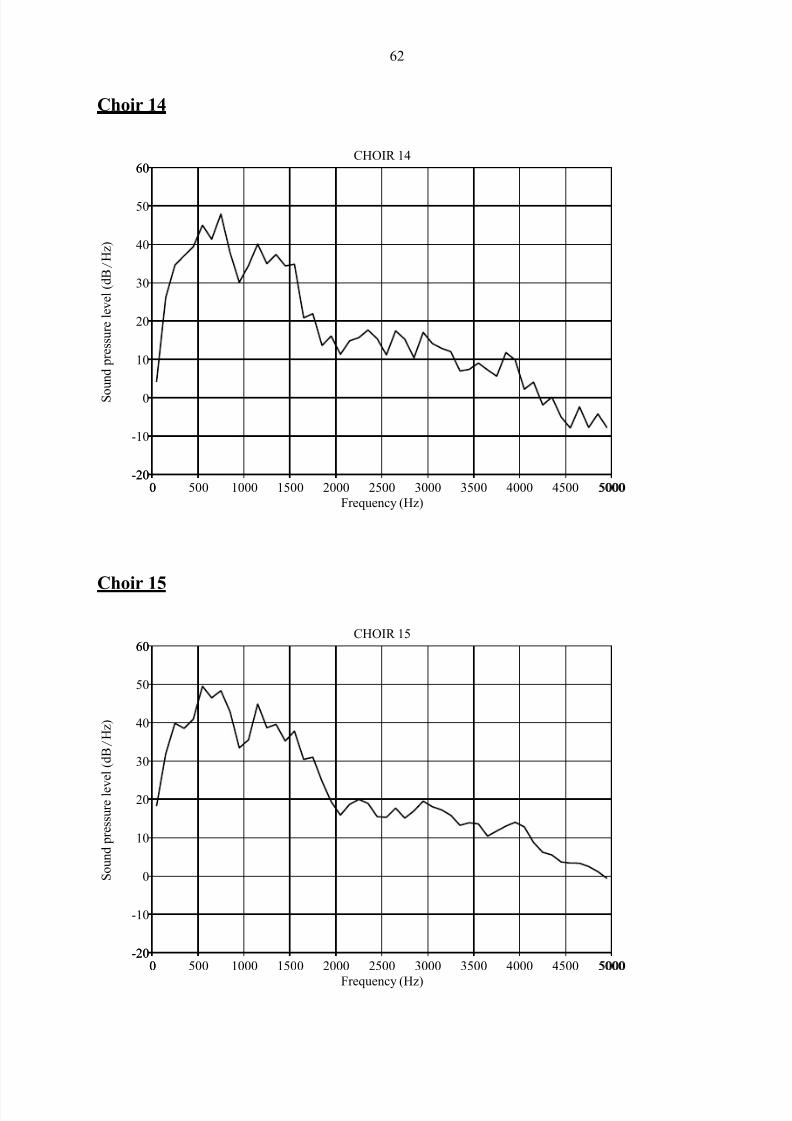
8/11/2019 FROM PHYSICS TO MUSIC.pdf
http://slidepdf.com/reader/full/from-physics-to-musicpdf 71/75
62
Choir 14
Frequency (Hz)
0 5000
S o
u n d p r e s s u r e l e v e l ( d B / H z )
-20
60
0 500 1000 1500 2000 2500 3000 3500 4000 4500 5000-20
-10
0
10
20
30
40
50
60CHOIR 14
Choir 15
Frequency (Hz)
0 5000
S o u n d p r e s s u r e l e v
e l ( d B / H z )
-20
60
0 500 1000 1500 2000 2500 3000 3500 4000 4500 5000-20
-10
0
10
20
30
40
50
60CHOIR 15

8/11/2019 FROM PHYSICS TO MUSIC.pdf
http://slidepdf.com/reader/full/from-physics-to-musicpdf 72/75
63
Choir 16
Frequency (Hz)
0 5000
S o
u n d p r e s s u r e l e v e l ( d B / H z )
-20
60CHOIR 16
-20
-10
0
10
20
30
40
50
60
0 500 1000 1500 2000 2500 3000 3500 4000 4500 5000
Choir 17
Frequency (Hz)0 5000
S o u n d p r e s s u r e l e v e l
( d B / H z )
-20
60CHOIR 17
0 500 1000 1500 2000 2500 3000 3500 4000 4500 5000
-20
-10
0
10
20
30
40
50
60

8/11/2019 FROM PHYSICS TO MUSIC.pdf
http://slidepdf.com/reader/full/from-physics-to-musicpdf 73/75
64
Choir 18
Frequency (Hz)
0 5000
S o
u n d p r e s s u r e l e v e l ( d B / H z )
-20
60CHOIR 18
0 500 1000 1500 2000 2500 3000 3500 4000 4500 5000-20
-10
0
10
20
30
40
50
60
Choir 19
Frequency (Hz)
0 5000
S o u n d p r e s s u r e l e
v e l ( d B / H z )
-20
60CHOIR 19
0 500 1000 1500 2000 2500 3000 3500 4000 4500 5000-20
-10
0
10
20
30
40
50
60

8/11/2019 FROM PHYSICS TO MUSIC.pdf
http://slidepdf.com/reader/full/from-physics-to-musicpdf 74/75
65
Choir 20
Frequency (Hz)
0 5000
S o
u n d p r e s s u r e l e v e l ( d B / H z )
-20
60CHOIR 20
0 500 1000 1500 2000 2500 3000 3500 4000 4500 5000-20
-10
0
10
20
30
40
50
60

8/11/2019 FROM PHYSICS TO MUSIC.pdf
http://slidepdf.com/reader/full/from-physics-to-musicpdf 75/75
66
ADDENDUM 4: CD CONTAI NING SOUND SAMPLES AND
SPREADSHEETS WITH RESULTS