From Newton's law to the linear Boltzmann equation without ...

From Newton’s law to the linear Boltzmannequation without cut-off

Nathalie Ayi (1)

(1)Universite Pierre et Marie Curie

27 Octobre 2017

Nathalie AYI Seminaire LJLL 27 Octobre 2017 1 / 35

Organisation of the talk

1- Physical and historical context of the result2- Difficulty in our framework3- Presentation of the usual tools for the proof4- Adaptation of the tools + new strategy in our context


Context

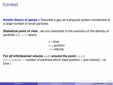
Kinetic theory of gases = Describe a gas as a physical system constituted ofa large number of small particles.

Statistical point of view : we are interested in the evolution of the density ofparticles f(t, x, v) where

t = timex = positionv = velocity

For all infinitesimal volume dxdv around the point (x, v):f(t, x, v)dxdv = number of particles which have position x and velocity v attime t.


Historical results:• A fundamental example, the Boltzmann equation (1872) = the evolution

equation for the density of particles of a sufficiently rarefied gas.

∂tf + v.∇xf︸︷︷︸free transport

= Q(f, f)︸︷︷︸localized binary collisions

• In the sixth problem of Hilbert (1900), idea = Boltzmann equation asan intermediate step in the transition between atomistic and contiuousmodel for gas dynamics.


The Boltzmann-Grad scaling

Change of scale = passage to the limit on one precise parameter of thesystem

Boltzmann-Grad scaling = N →∞, Nεd−1 = 1.

Rarefied gas : Nεd � 1, not too much collisions.


Historical Panorama

Lanford proved the derivation of the Boltzmann equation from systems ofparticles in the context of hard-spheres (1975).

Particles bounces off according to the laws of elastic reflection.


Proof recently improved by Gallagher, Saint-Raymond and Texier, Pulvirenti,Saffirio and Simonella in the context of hard-spheres and short rangepotentials.

(Figure: The Boltzmann equation and its application, Cercignani.)

Our context: infinite-range potentials.


The Boltzmann equation without cut-off

The Boltzmann equation

∂tf + v.∇xf =∫

Rd

∫Sd−1

(f ′f ′1 − ff1)b(v − v1, ν)dνdv1

b(v − v1, ν) = cross-section, θ = deviation angle

b(v − v1, ν) = b(|v − v1|, cos(θ))

integrability with respect to θ ⇒ Boltzmann with cut-offnon-integrability with respect to θ ⇒ Boltzmann without cut-off

ExampleInverse-power law potentials: Φ(r) = 1

rs−1 , s > 2. The cross-sectionsatisfies

b(|v − v1|, cos θ) = q(cosθ)|v − v1|γ ,

sind−2θq(cos θ) ∼ Cθ−1−α, α > 0


Hard-spheres, Short range potentials⇒ Boltzmann with cut-off

Difficulty = infinite range potential⇒ singularity due to grazing collisions⇒ Boltzmann without cut-off

Intuitive idea= use of compensation between gain and loss terms

f(v)f(v1) ≈ f(v′)f(v′1)

The Boltzmann equation

∂tf + v.∇xf =∫

Rd

∫Sd−1

(f ′f ′1 − ff1)b(v − v1, ν)dνdv1


The Hard-spheres case

Microscopic Model: for i ∈ {1, . . . , N},dxidt

= vi, xi, vi ∈ Rd

dvidt

= 0, |xi(t)− xj(t)| > ε.

If |xi − xj | = ε,v′i = vi + ((vj − vi) · ν)νv′j = vj − ((vj − vi) · ν)ν

Appropriate quantities:

fN (t, ZN ) = distribution function of N particles

with zi = (xi, vi), ZN = (z1, . . . , zN ). Marginal of order one :

f(1)N (t, x1, v1) =

∫fNdx2 . . . dxNdv2 . . . dvN .


Formal justification of the limit

Liouville equation + Green formula⇒

∂tf(1)N + v1 · ∇x1f

(1)N = (N − 1)εd−1

∫Sd−1×Rd

[f

(2)N (t, x1, v

′1, x1 + εν, v′2)

−f (2)N (t, x1, v1, x1 − εν, v2)

]((v2 − v1) · ν)+dνdv2.

N →∞,

∂tf + v1 · ∇x1f =∫

Sd−1×Rd

[f (2)(t, x1, v

′1, x1, v

′2)

−f (2)(t, x1, v1, x1, v2)]

((v2 − v1) · ν)+dνdv2

If f (2)(Z2) = f(z1)f(z2)⇒ the Boltzmann equation.

Key notion = Propagation of chaos.


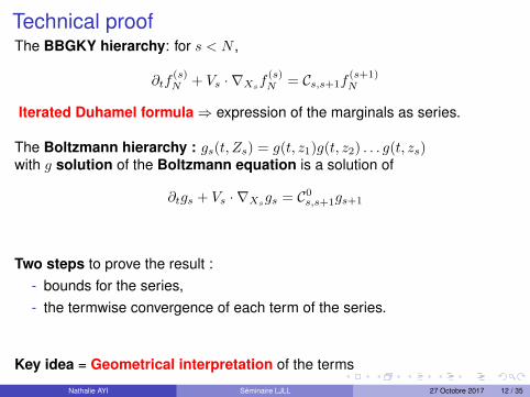
Technical proofThe BBGKY hierarchy: for s < N ,

∂tf(s)N + Vs · ∇Xsf

(s)N = Cs,s+1f

(s+1)N

Iterated Duhamel formula⇒ expression of the marginals as series.

The Boltzmann hierarchy : gs(t, Zs) = g(t, z1)g(t, z2) . . . g(t, zs)with g solution of the Boltzmann equation is a solution of

∂tgs + Vs · ∇Xsgs = C0s,s+1gs+1

Two steps to prove the result :- bounds for the series,- the termwise convergence of each term of the series.

Key idea = Geometrical interpretation of the terms


Iterated Duhamel’s formula.Duhamel’s formula:

f(s)N (t) = Ts(t)f (s)

N (0) +∫ t

0Ts(t− t1)Cs,s+1f

(s+1)N (t1)dt1.

The BBGKY series:

f(s)N (t) =

N−s∑n=0

∫ t

0

∫ t1

0. . .

∫ tn−1

0Ts(t−t1)Cs,s+1Ts+1(t1−t2)Cs+1,s+2 . . . Ts+n(tn)

f(s+n)N (0)dtn . . . dt1.

The Boltzmann series:

g(s)(t) =∑n≥0

∫ t

0

∫ t1

0. . .

∫ tn−1

0T 0s (t−t1)C0

s,s+1T 0s+1(t1−t2)C0

s+1,s+2 . . . T 0s+n(tn)

g(s+n)(0)dtn . . . dt1

Strategy: Notion of pseudo-trajectories.Nathalie AYI Seminaire LJLL 27 Octobre 2017 13 / 35

pt

pt1

pt20

v1

v2

v3

FIGURE : Representation of a pseudo-trajectory associated to the term∫ t

0

∫ t1

0T1(t− t1)C1,2T2(t1 − t2)C2,3T3(t2)f (3)

N (0)dt2dt1 for the BBGKY hierar-

chy.


pt

pt1

pt20

v1

v2

v3

FIGURE : Representation of a pseudo-trajectory associated to the term∫ t

0

∫ t1

0T 0

1 (t− t1)C01,2T 0

2 (t1 − t2)C02,3T 0

3 (t2)f (3)N (0)dt2dt1 for the Boltzmann hi-

erarchy.

Strategy: Coupling of the pseudo-trajectories.


Recollision

pt

pt∗

pt1

pt20

v1

v2

v3

Figure: An example of a recollision between particles 1 and 2 at time t∗.

Strategy: Geometrical control of the recollisions


Strategy of the proof and limit

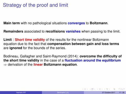
Main term with no pathological situations converges to Boltzmann.

Remainders associated to recollisions vanishes when passing to the limit.

Limit : Short time validity of the results for the nonlinear Boltzmannequation due to the fact that compensation between gain and loss termsare ignored for the bounds of the series.

Bodineau, Gallagher and Saint-Raymond (2014): overcome the difficulty ofthe short time validity in the case of a fluctuation around the equilibrium⇒ derivation of the linear Boltzmann equation.


The infinite range potential case

Difficulty = The singularity prevents the single-use of Lanford’s approach.

Ideas =- framework of perturbation around the equilibrium,- ∇Φ = ∇φ>R +∇Φ<R,- new terms with presence of derivatives⇒ weak approach.


ResultMicroscopic Model: for i ∈ {1, . . . , N}, xi ∈ Td, vi ∈ Rd,

dxidt

= vi,

dvidt

= −1ε

∑j 6=i∇Φ(xi − xj

ε).

Tagged particle in a gas at equilibrium:

f0N (ZN ) := MN,β(ZN )ρ0(x1)

ρ0 density of probability on Td, MN,β Gibbs measure: for β > 0

MN,β(ZN ) := 1ZN

(β

2π

)dN/2exp(−βHN (ZN ))

with HN (ZN ) :=∑

1≤i≤N

12 |vi|

2 +∑

1≤i<j≤NΦ((xi − xj

ε).


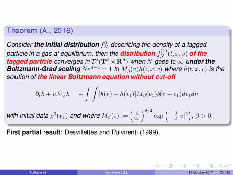
Theorem (A., 2016)

Consider the initial distribution f0N describing the density of a tagged

particle in a gas at equilibrium, then the distribution f(1)N (t, x, v) of the

tagged particle converges in D′(Td ×Rd) when N goes to∞ under theBoltzmann-Grad scaling Nεd−1 = 1 to Mβ(v)h(t, x, v) where h(t, x, v) is thesolution of the linear Boltzmann equation without cut-off

∂th+ v.∇xh = −∫ ∫

[h(v)− h(v1)]Mβ(v1)b(v − v1)dv1dν

with initial data ρ0(x1) and where Mβ(v) :=(β

2π

)d/2exp

(−β2 |v|

2)

, β > 0.

First partial result: Desvillettes and Pulvirenti (1999).


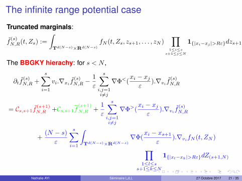
The infinite range potential case

Truncated marginals:

f(s)N,R(t, Zs) :=

∫Td(N−s)×Rd(N−s)

fN (t, Zs, zs+1, . . . , zN )∏

1≤i≤ss+1≤j≤N

1{|xi−xj |>Rε}dzs+1 . . . dzN

The BBGKY hierachy: for s < N ,

∂tf(s)N,R +

s∑i=1

vi.∇xi f(s)N,R −

1ε

s∑i,j=1i 6=j

∇Φ<(xi − xjε

).∇vi f(s)N,R

= Cs,s+1f(s+1)N,R +Cs,s+1f

(s+1)N,R + 1

ε

s∑i,j=1i 6=j

∇Φ>(xi − xjε

).∇vi f(s)N,R

+ (N − s)ε

s∑i=1

∫Td(N−s)×Rd(N−s)

∇Φ(xi − xs+1

ε).∇vifN (t, ZN )∏

1≤l≤ss+1≤k≤N

1{|xl−xk|>Rε}dZ(s+1,N)


Duhamel’s formula:

f(s)N,R(t, Zs) = Ss(t)f (s)

N,R(0, Zs)

+∫ t

0Ss(t− t1)Cs,s+1f

(s+1)N,R (t1, Zs)dt1

+∫ t

0Ss(t− t1)Cs,s+1f


+1ε

s∑i,j=1i 6=j

∫ t

0Ss(t− t1)

[∇Φ>(xi − xj

ε).∇vi f

(s)N,R

](t1, Zs)dt1

+(N − s)ε

s∑i=1

∫ t

0Ss(t− t1)

[∫Td(N−s)×Rd(N−s)

∇Φ(xi − xs+1

ε).∇vifN

∏1≤l≤s

s+1≤k≤N

1{|xl−xk|>Rε}dZ(s+1,N)

(t1, Zs)dt1


Obstacles to the convergence

Four possible obstacles to the convergence:- the very long-range interactions,- clusters (or multiple simultaneous interactions),- the presence of recollisions,- super-exponential collision process.


The pruning process

Definition

Let τ > 0 and denote t := Kτ for some large integer K. We split [0, t] into∪1≤k≤K [(k − 1)τ, kτ ]. We call a collision tree “of controlled size” a collisiontree such that it has less than nk = 2k branch points on the interval[t− kτ, t− (k − 1)τ ].We call a collision tree with super-exponential growth a collision treewhich does not satisfy the above property.


Figure: A super-exponential tree (Source: The Brownian Motion as the limitof a deterministic system of hard-spheres, Bodineau et al).


Obstacles to the convergence

Four possible obstacles to the convergence:- the very long-range interactions,- clusters (or multiple simultaneous interactions),- the presence of recollisions,- super-exponential collision process.

Iteration on the term:∫ t

0Ss(t− t1)Cs,s+1f

(s+1)N,R (t1, Zs)dt1.

New strategy = truncations at each iteration step.


Truncations to avoid pathological situations

Elimination of recollisions: notion of good configurations.

Definition

The set of good configuration Gk(ε0) is defined as follows:

Gk(ε0) := {Zk ∈ Tdk ×Rdk|∀u ∈ [0, t] ∀i 6= j d(xi − uvi, xj − uvj) ≥ ε0}.

Bad sets to remove geom(s+k) :s+ k − 1 particles in a good configuration −→ after a delay δ, the s+ kparticles are in a good configuration.


Truncations associated to the elimination of recollisions:- cutting off the energy of the system via a smooth function such that

χE2(x) =

{1 if |x| ≤ E2

0 if |x| ≥ E2 + 1.

χE2(Hk(Zk)) := χ{Hk(Zk)≤E2} for all integer k,

- separation of the collision times by δ.Additional truncation:

- small relative velocities via a smooth function such that

χη(x) ={

0 if |x| ≤ η/21 if |x| ≥ η

χ{∀i∈{1,...,k}|vi−vk+1|≥η} :=k∏i=1

χη(vi − vk+1).


One iteration:

∫ t

0Ss(t− t1)Cs,s+1f


=∫ t

t−δSs(t− t1)Cs,s+1f


+∫ t−δ

0Ss(t− t1)Cs,s+1

(1− χ{Hs+1(Zs+1)≤E2}

)f


+∫ t−δ

0Ss(t− t1)Cs,s+1χ{Hs+1(Zs+1)≤E2}χgeom(s+1)f


+∫ t−δ

0Ss(t− t1)Cs,s+1χ{Hs+1(Zs+1)≤E2}

(1− χgeom(s+1)

) (1− χ{∀i∈{1,...,s}|vi−vs+1|≥η}

)f


+∫ t−δ

0Ss(t− t1)Cs,s+1χ{Hs+1(Zs+1)≤E2}

(1− χgeom(s+1)

)χ{∀i∈{1,...,s}|vi−vs+1|≥η}

f(s+1)N,R (t1, Zs)dt1.


Definition of the operators:

Qs,s(t) := Ss(t)

Qs,s+n(t) :=∫ t−δ

0

∫ t1−δ

0. . .

∫ tn−1−δ

0Ss(t− t1)Cs,s+1χHs+1

(1− χgeom(s+1)

)χηs+1 . . .

. . .Ss+n−1(tn−1 − tn)Cs+n−1,s+nχHs+n

(1− χgeom(s+n)

)χηs+nSs+n(tn)dtn . . . dt1.

Remainders associated to the long-range part:

rPot,as,m+1(0, t, Zs) :=m∑n=0

∫ t−nδ

0Qs,s+n(t− tn+1)

1ε

s+n∑i,j=1i 6=j

[∇Φ>(

xi − xjε

).∇vi f(s+n)N,R

](tn+1, Zs)dtn+1


rPot,bs,m+1(0, t, Zs) :=m∑n=0

∫ t−nδ

0Qs,s+n(t− tn+1)

(N − (s+ n))ε

s+n∑i=1

[∫Td(N−(s+n))×Rd(N−(s+n))

∇Φ(xi − xs+n+1

ε).∇vifN

∏1≤l≤s+n

s+n+1≤k≤N

1{|xl−xk|>Rε}dZ(s+n,N)

(tn+1, Zs)dtn+1.


Control of the new terms

Maximum Principle for the Liouville equation⇒ A priori estimates on thetruncated marginals.

Problem: Control on the marginals but not on the derivatives of the marginals⇒Weak approach.


Advantage of the iteration method

no pathological situations⇒ easy to pass from Zm(tm) to z (state ofparticle 1 at time t) via changes of variables such as

Td ×Rd × [0, t− δ]× Sd−1 ×Rd × · · · × [0, tm−1 − δ]× Sd−1 ×Rd → T(m+1)d ×R(m+1)d

(z, t1, ν2, v2, . . . , tm, νm+1, vm+1) 7→ Zm+1 = Zm+1(tm).

Key point: z Lipschitz function of (x1, v1, . . . , xm+1, vm+1)

Tools to prove it: study of the reduced dynamics- bound on the microscopic time of interaction thanks to the lower

bound on relative velocites,- use of the Cauchy-Lipschitz theorem, ∇Φ being Lipschitz,- Lipschitz character of the collision times.


Proposition

The function (x1, v1, . . . , xk+1, vk+1) 7→ z = z(x1, v1, . . . , xk+1, vk+1), where(x1, v1, . . . , xk+1, vk+1) is the state of the k + 1 particles after k collisionsat time t+k+1 (i.e. before the k + 1-th collision) on a pseudo-trajectory is a

(CR,η,ε)k-Lipschitz function with CR,η,ε = CReCR3/η

η | cos(π2 − ε

)|ε

and C is a constant

which can only depend on ∇Φ.

Lipschitz control associated to the pseudo-trajectories =⇒ bound of theremainder associated to the long-range part controlled by(

eCR3η

)2K+1

‖∇Φ>‖∞.

Limit of the approach: Very decreasing potentials.


Thank you for your attention.


From Newton's law to the linear Boltzmann equation without ...

Documents

Transcript of From Newton's law to the linear Boltzmann equation without ...