From Monte Carlo to Bayes Theory: The Role of Uncertainty ... Bayes To Monte_Carlo AFES.pdf · From...

www.senergyworld.com

From Monte Carlo to Bayes Theory: The Role of Uncertainty in Petrophysics.

Simon Stromberg

Global Technical Head of Petrophysics

Senergy

Subsurface Characterisation

The main goal of the oil-industry geoscience professional is

to characterise the complete range of possible

configurations of the subsurface for a given set of data

and related analogues.

This characterisation of the subsurface should lead to a

comprehensive description of uncertainty that leads to the

complete disclosure of the financial risk of further

exploration, appraisal or development of a potential

hydrocarbon resource.

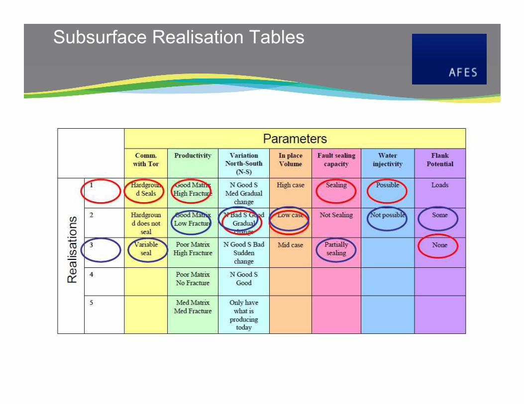
Subsurface Realisation Tables

Petrophysical workflows

Calculate

Volume of

Clay

Calculate Clay

Corrected

Porosity

Calculate Clay

Corrected

Saturation

Apply cut-offs for

net sand,

reservoir and pay

and averages

Volume of Clay

Effective and Total

Porosity

Effective and Total

Water Saturation

Average Vcl, Por, Phi

And HPVOL

Petrophysical Base Case Interpretation

Methods of Uncertainty Analysis

• Parameter sensitivity analysis

• Partial derivative analysis

• Monte Carlo Simulation

• Bayesian Analysis for Diagnostic Reliability

Sensitivity Analysis of Input Parameters – Single Parameter

• For example:

• Volume of clay cut-off

for net reservoir

• If VCL <= 0.3 and

• If PHIE >= 0.1 then

• The interval is flagged

as net reservoir

Sensitivity Analysis of Input Parameters – Single Parameter

Sensitivity Analysis of Input Parameters – Single Parameters

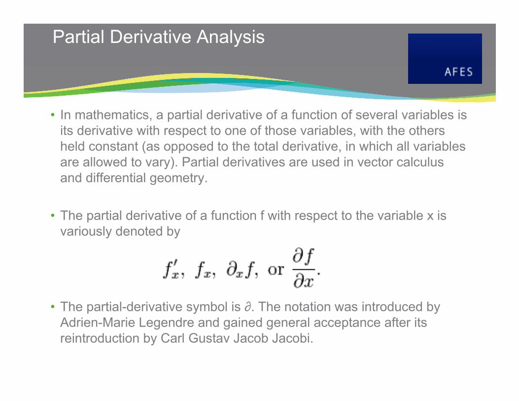
Partial Derivative Analysis

• In mathematics, a partial derivative of a function of several variables is

its derivative with respect to one of those variables, with the others

held constant (as opposed to the total derivative, in which all variables

are allowed to vary). Partial derivatives are used in vector calculus

and differential geometry.

• The partial derivative of a function f with respect to the variable x is

variously denoted by

• The partial-derivative symbol is ∂. The notation was introduced by

Adrien-Marie Legendre and gained general acceptance after its

reintroduction by Carl Gustav Jacob Jacobi.

Partial Derivative Analysis – Example

• Volume of a cone is:

• The partial derivative of the volume with respect to the

radius is

• Which describes the rate at which the volume changes

with change in radius if the height is kept constant.

Partial Derivative Analysis for Waxman-Smits Equation for Saturation

( ) ( )

( ) ( ) ( )SwRt

A

RwA

Sw

QvBRwRt

n

m

n

FQvBRwSwnSwE

E

SwFRw

n

Sw

E

FRw

m

Sw

AE

FRw

A

Sw

E

FRwmSw

RwE

Sw

Rw

Sw

RtE

Rw

Rt

Sw

nn

Swm

m

SwA

A

SwSwRw

Rw

SwRt

Rt

SwSw

m

Sw

⋅⋅

⋅

⋅

⋅⋅

+⋅

−

−

−

=⋅⋅+⋅−+=

⋅⋅−=

∂∂⋅⋅

−=∂∂

⋅⋅

=∂

∂

⋅⋅⋅

−=∂

∂⋅

=∂∂

⋅−=

∂∂

⋅∂

∂+

⋅∂∂

+

⋅∂

∂+

⋅

∂∂

+

⋅∂∂

+

⋅∂∂

=

=

2

2

222222

1

;1

ln;

ln;

;;

1

φ

φ

φφφ

δδδδφφ

δδδ

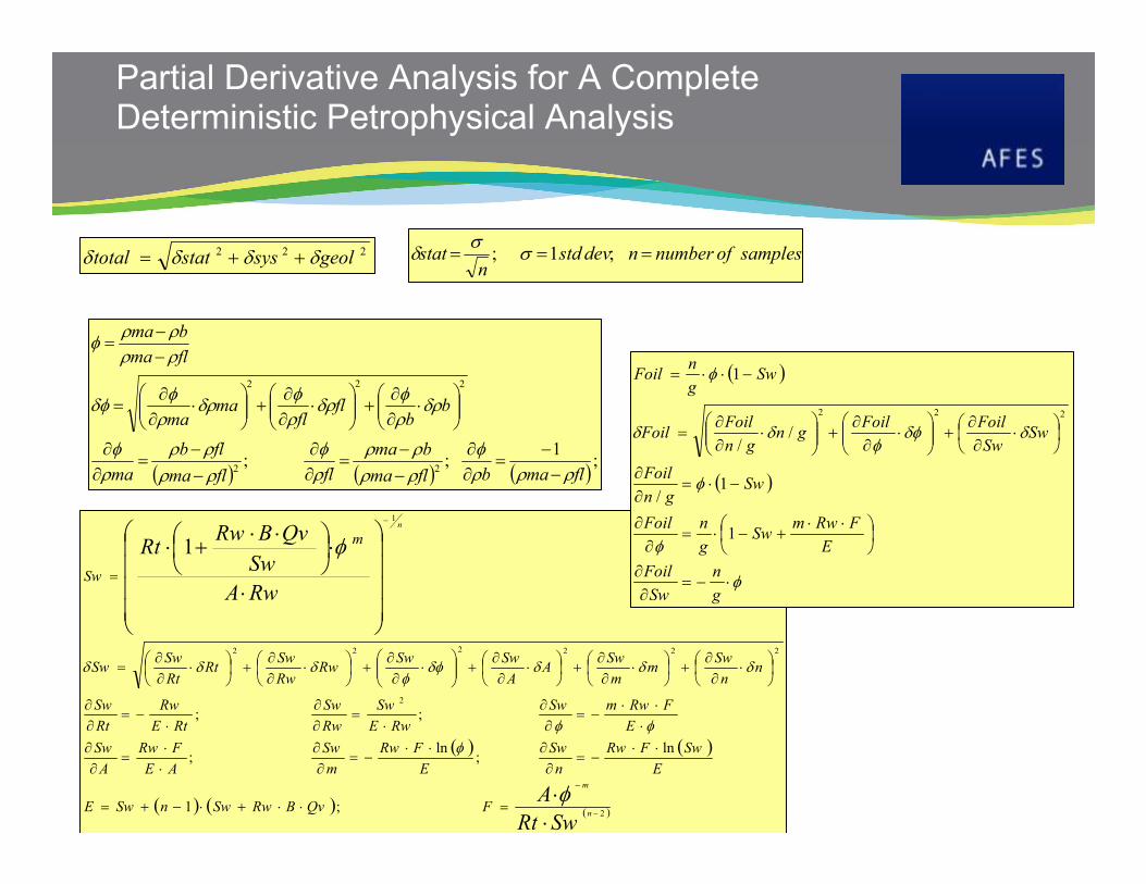
Partial Derivative Analysis for A Complete Deterministic Petrophysical Analysis

( ) ( )

( ) ( ) ( )SwRt

A

RwA

Sw

QvBRwRt

n

m

n

FQvBRwSwnSwE

E

SwFRw

n

Sw

E

FRw

m

Sw

AE

FRw

A

Sw

E

FRwmSw

RwE

Sw

Rw

Sw

RtE

Rw

Rt

Sw

nn

Swm

m

SwA

A

SwSwRw

Rw

SwRt

Rt

SwSw

m

Sw

⋅⋅

⋅

⋅

⋅⋅

+⋅

−

−

−

=⋅⋅+⋅−+=

⋅⋅−=

∂∂⋅⋅

−=∂

∂⋅⋅

=∂

∂

⋅⋅⋅

−=∂

∂⋅

=∂∂

⋅−=

∂∂

⋅∂

∂+

⋅∂

∂+

⋅∂

∂+

⋅

∂∂

+

⋅∂∂

+

⋅∂∂

=

=

2

2

222222

1

;1

ln;

ln;

;;

1

φ

φ

φφφ

δδδδφφ

δδδ

( ) ( ) ( );

1;;

22

222

flmabflma

bma

flflma

flb

ma

bb

flfl

mama

flma

bma

ρρρφ

ρρρρ

ρφ

ρρρρ

ρφ

δρρφ

δρρφ

δρρ

φδφ

ρρρρ

φ

−−

=∂∂

−

−=

∂∂

−

−=

∂∂

⋅

∂∂

+

⋅

∂∂

+

⋅

∂∂

=

−−

=

( )

( )

φ

φ

φ

δδφφ

δδ

φ

⋅−=∂

∂

⋅⋅+−⋅=

∂∂

−⋅=∂∂

⋅∂

∂+

⋅

∂∂

+

⋅

∂∂

=

−⋅⋅=

g

n

Sw

Foil

E

FRwmSw

g

nFoil

Swgn

Foil

SwSw

FoilFoilgn

gn

FoilFoil

Swg

nFoil

1

1/

//

1

222

222 geolsysstattotal δδδδ ++= samplesofnumberndevstdn

stat === ;1; σσ

δ

Partial Derivative – Input Data

Zonal Averages

well zone gross net n2g por Sw

1 HSGHL 45.6 30.8 0.676 0.264 0.364

2 HSGHL 19.9 11.9 0.595 0.243 0.478

4 HSGHL 44.8 22.2 0.497 0.256 0.347

5 HSGHL 31.3 11.7 0.376 0.266 0.319

6 HSGHL 5.7 0.0 0.000 0.000 1.000

7 HSGHL 40.0 12.2 0.305 0.239 0.292

8 HSGHL 46.8 16.2 0.345 0.270 0.393

Sumavs

Partial Derivative – Input Uncertainty

Field: Zone:

parameter value 1 std dev part error % error parameter value 1 std dev part error % error

count 6 count 6

w average 0.258 0.013 w average 0.636 0.065

δδδδstat 0.005 2.0% δδδδstat 0.027 4.2%

rhob 2.224 0.010 -0.006 -2.3% Rt 10.723 1.072 -0.026 -4.1%

rhoma 2.650 0.010 0.004 1.7% Rw 0.300 0.060 0.021 3.4%

rhofl 1.000 0.020 0.003 1.2% por 0.258 0.010 -0.017 -2.7%

A 1.000 0.001 0.000 0.0%

m 1.800 0.150 0.052 8.2%

n 2.000 0.200 0.052 8.2%

B 7.000 1.400 -0.030 -4.7%

Qv 0.245 0.025 -0.015 -2.4%

δδδδsys 0.008 3.2% δδδδsys 0.089 14.1%

δδδδgeol 0.000 0.0% δδδδgeol 0.000 0.0%

average 0.258 δδδδtotal 0.010 3.8% average 0.636 δδδδtotal 0.093 14.7%

count 7 count 6

w average 0.449 0.222 w average 0.074 0.022

δδδδstat 0.084 18.7% n/g 0.449 0.131 0.021 29.1%

por 0.258 0.010 0.005 6.5%

Sh 0.636 0.093 -0.011 -14.7%

δδδδgeol 0.100 22.3% δδδδsys 0.024 33.2%

average 0.449 δδδδtotal 0.131 29.1% average 0.074 δδδδtotal 0.024 33.2%

Foil=n/g*por*Shnet/gross

Porosity Hydrocarbon Saturation

Partial Derivative Analysis Results

porosity Hydrocarbon Saturation

Uncertainty (Normal) Distribution Curves

net/gross Foil

0.0

0.1

0.2

0.3

0.4

0.5

0.6

0.7

0.8

0.9

1.0

0.00 0.10 0.20 0.30 0.40

porosity

dis

trib

uti

on

0.0

5.0

10.0

15.0

20.0

25.0

30.0

35.0

40.0

45.0

avg=0.258, std=0.010, std=3.8% µ−3σ=0.229, µ+3σ=0.287

0.0

0.1

0.2

0.3

0.4

0.5

0.6

0.7

0.8

0.9

1.0

0.00 0.20 0.40 0.60 0.80 1.00

Sh

dis

trib

uti

on

0.0

0.5

1.0

1.5

2.0

2.5

3.0

3.5

4.0

4.5

avg=0.636, std=0.093, std=14.7% µ−3σ=0.356, µ+3σ=0.916

0.0

0.1

0.2

0.3

0.4

0.5

0.6

0.7

0.8

0.9

1.0

0.00 0.05 0.10 0.15 0.20 0.25 0.30

Foil

dis

trib

uti

on

0.0

2.0

4.0

6.0

8.0

10.0

12.0

14.0

16.0

18.0

avg=0.074, std=0.024, std=33.2% µ−3σ=0.000, µ+3σ=0.147

0.0

0.1

0.2

0.3

0.4

0.5

0.6

0.7

0.8

0.9

1.0

0.00 0.20 0.40 0.60 0.80 1.00net/gross

dis

trib

uti

on

0.0

0.5

1.0

1.5

2.0

2.5

3.0

3.5

avg=0.449, std=0.131, std=29.1% µ−3σ=0.057, µ+3σ=0.840

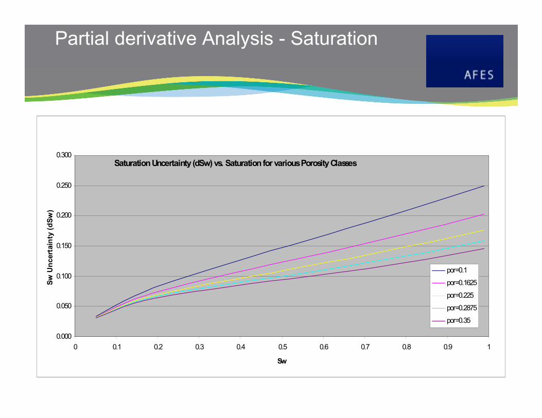
Partial derivative Analysis - Saturation

Saturation Uncertainty (dSw) vs. Saturation for various Porosity Classes

0.000

0.050

0.100

0.150

0.200

0.250

0.300

0 0.1 0.2 0.3 0.4 0.5 0.6 0.7 0.8 0.9 1

Sw

Sw

Un

cert

ain

ty (

dS

w)

por=0.1

por=0.1625

por=0.225

por=0.2875

por=0.35

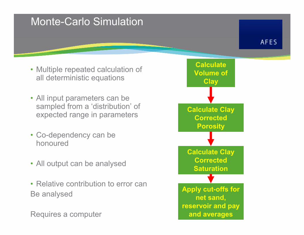
Monte-Carlo Simulation

• Multiple repeated calculation of all deterministic equations

• All input parameters can be sampled from a ‘distribution’ of expected range in parameters

• Co-dependency can be honoured

• All output can be analysed

• Relative contribution to error can

Be analysed

Requires a computer

Calculate

Volume of

Clay

Calculate Clay

Corrected

Porosity

Calculate Clay

Corrected

Saturation

Apply cut-offs for

net sand,

reservoir and pay

and averages

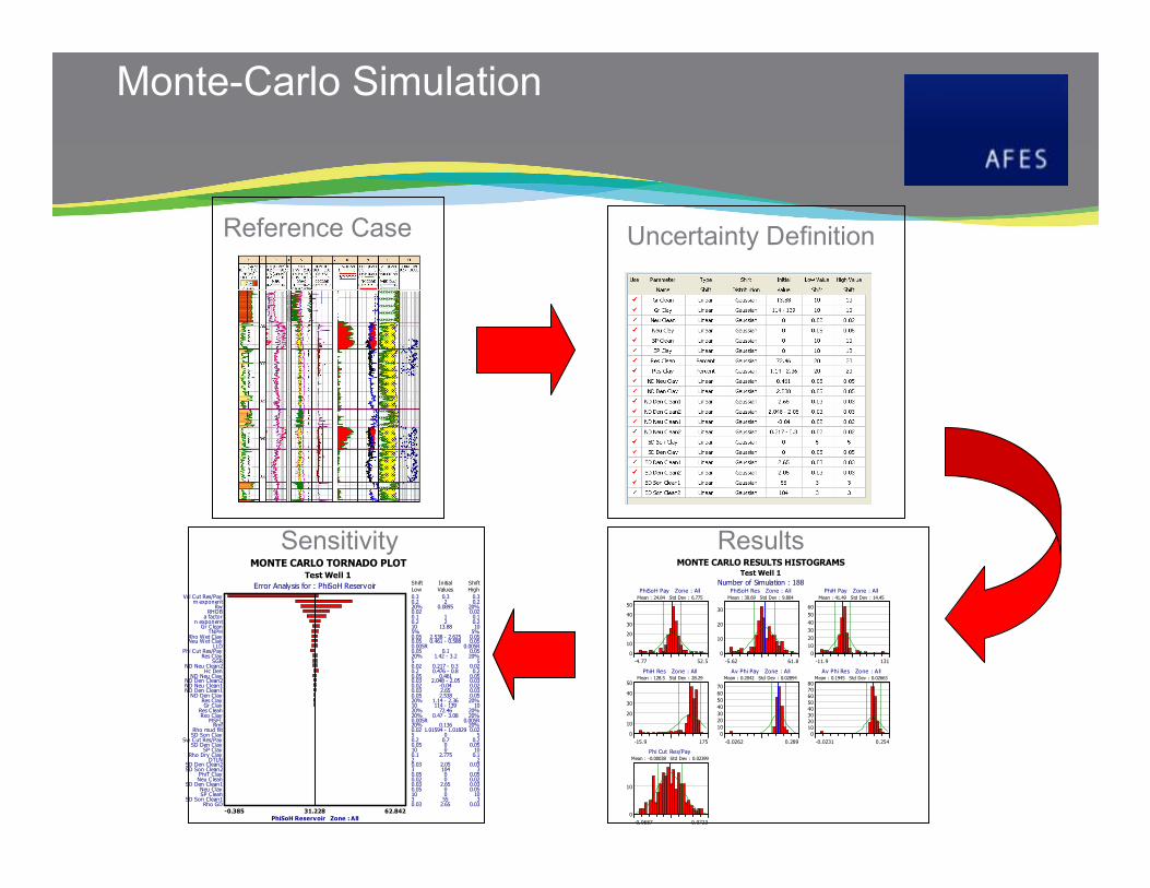
Monte-Carlo Simulation

Reference Case Uncertainty Definition

MONTE CARLO RESULTS HISTOGRAMSTest Well 1

Number of Simulation : 188PhiSoH Pay Zone : AllMean : 24.84 Std Dev : 6.775

0

10

20

30

40

50

-4.77 52.5

PhiSoH Res Zone : AllMean : 30.69 Std Dev : 9.804

0

10

20

30

-5.62 61.8

PhiH Pay Zone : A llMean : 41.49 Std Dev : 14.45

0

10

20

30

40

50

60

-11.9 131

PhiH Res Zone : AllMean : 128.5 Std Dev : 28.29

0

10

20

30

40

50

-15.9 175

Av Phi Pay Zone : AllMean : 0.2042 Std Dev : 0.02894

0

10

20

30

40

50

60

70

-0.0262 0.289

Av Phi Res Zone : A llMean : 0.1945 Std Dev : 0.02663

01020304050

607080

-0.0231 0.254

Phi Cut Res/PayMean : -0.00038 Std Dev : 0.02399

0

10

-0.0687 0.0723

ResultsMONTE CARLO TORNADO PLOT

Test Well 1

Error Analysis for : PhiSoH Reservoir

Rho GDSD Son Clean1

SP CleanNeu C lay

SD Den Clean1Neu C leanPhiT C lay

SD Son Clean2SD Den Clean2

DTLNRho Dry C lay

SP C laySD Den C lay

Sw Cut Res/PaySD Son C layRho mud filt

RmfMSFL

Rxo C layRes CleanGr C layRes C lay

ND Den C layND Den Clean1ND Neu Clean1ND Den Clean2ND Neu C lay

Hc DenND Neu Clean2

SGRRes C lay

Phi Cut Res/PayLLD

Neu Wet C layRho Wet C lay

TNPHGr Clean

n exponenta factorRHOB

Rwm exponent

Vcl Cut Res/Pay

0.03 2.65 0.033 55 310 0 100.05 0 0.050.03 2.65 0.030.02 0 0.020.05 0 0.053 104 30.03 2.05 0.032 20.1 2.775 0.110 0 100.05 0 0.050.2 0.7 0.25 0 50.02 1.01594 - 1.01829 0.0220% 0.136 20%0.005R 0.005R20% 0.47 - 3.08 20%20% 72.46 20%10 114 - 139 1020% 1.14 - 2.36 20%0.05 2.538 0.050.03 2.65 0.030.02 -0.04 0.020.03 2.048 - 2.05 0.030.05 0.461 0.050.2 0.476 - 0.8 0.20.02 0.217 - 0.3 0.025 520% 1.42 - 3.2 20%0.05 0.1 0.050.005R 0.005R0.05 0.461 - 0.588 0.050.05 2.538 - 2.625 0.055% 5%10 13.88 100.2 2 0.20.1 1 0.10.02 0.0220% 0.0895 20%0.2 2 0.20.3 0.3 0.3

ShiftLow

InitialValues

ShiftHigh

31.228-0.385 62.842

PhiSoH Reservoir Zone : All

Sensitivity

Models and Equations

ResultsMONTE CARLO RESULTS HISTOGRAMS

Test Well 1

Number of Simulation : 408PhiSoH Pay Zone : AllMean : 24.86 Std Dev : 6.198

0

20

40

60

80

100

-5.49 60.4

HPVOL (ft)

SensitivityMONTE CARLO TORNADO PLOT

Test Well 1

Error Analysis for : PhiSoH Pay

DTLN

Rho mud filt

Rho GD

Rho Dry C lay

PhiT C lay

Res Clean

MSFL

Rxo Clay

ND Den Clay

Res C lay

ND Den Clean1

Rmf

Gr C lay

ND Neu Clean1

ND Den Clean2

ND Neu Clay

ND Neu Clean2

Phi Cut Res/Pay

Res C lay

TNPH

LLD

Hc Den

SGR

Neu Wet C lay

Rho Wet C lay

Gr Clean

a factor

n exponent

RHOB

Rw

m exponent

Sw Cut Res/Pay

Vcl Cut Res/Pay

2 2

0.02 1.01594 - 1.01829 0.02

0.03 2.65 0.03

0.1 2.775 0.1

0.05 0 0.05

20% 72.46 20%

0.005R 0.005R

20% 0.47 - 3.08 20%

0.05 2.538 0.05

20% 1.14 - 2.36 20%

0.03 2.65 0.03

20% 0.136 20%

10 114 - 139 10

0.02 -0.04 0.02

0.03 2.048 - 2.05 0.03

0.05 0.461 0.05

0.02 0.217 - 0.3 0.02

0.05 0.1 0.05

20% 1.42 - 3.2 20%

5% 5%

0.005R 0.005R

0.2 0.476 - 0.8 0.2

5 5

0.05 0.461 - 0.588 0.05

0.05 2.538 - 2.625 0.05

10 13.88 10

0.1 1 0.1

0.2 2 0.2

0.02 0.02

20% 0.0895 20%

0.2 2 0.2

0.2 0.7 0.2

0.3 0.3 0.3

ShiftLow

InitialValues

ShiftHigh

9.9920.023 19.962

PhiSoH Pay Zone : 3

Bayesian Analysis For Reliability

Bayes allows modified probabilities to be calculated based on

1. The expected rate of occurrence in nature

2. A diagnostic test that is less than 100% reliable

For example

• There is a 1:10,000 (0.0001%) occurrence of a rare disease in the population

• There is a single test of the disease that is 99.99% accurate

• A patient is tested positive for that disease

• What is the likelihood that the patient tested positive actually has the disease?

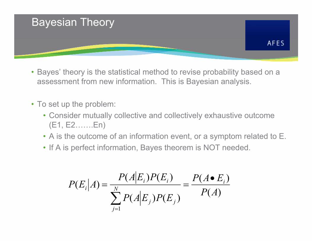
Bayesian Theory

• Bayes’ theory is the statistical method to revise probability based on a

assessment from new information. This is Bayesian analysis.

• To set up the problem:

• Consider mutually collective and collectively exhaustive outcome

(E1, E2…….En)

• A is the outcome of an information event, or a symptom related to E.

• If A is perfect information, Bayes theorem is NOT needed.

)(

)(

)()(

)()()(

1

AP

EAP

EPEAP

EPEAPAEP i

N

j

jj

ii

i

•==

∑=

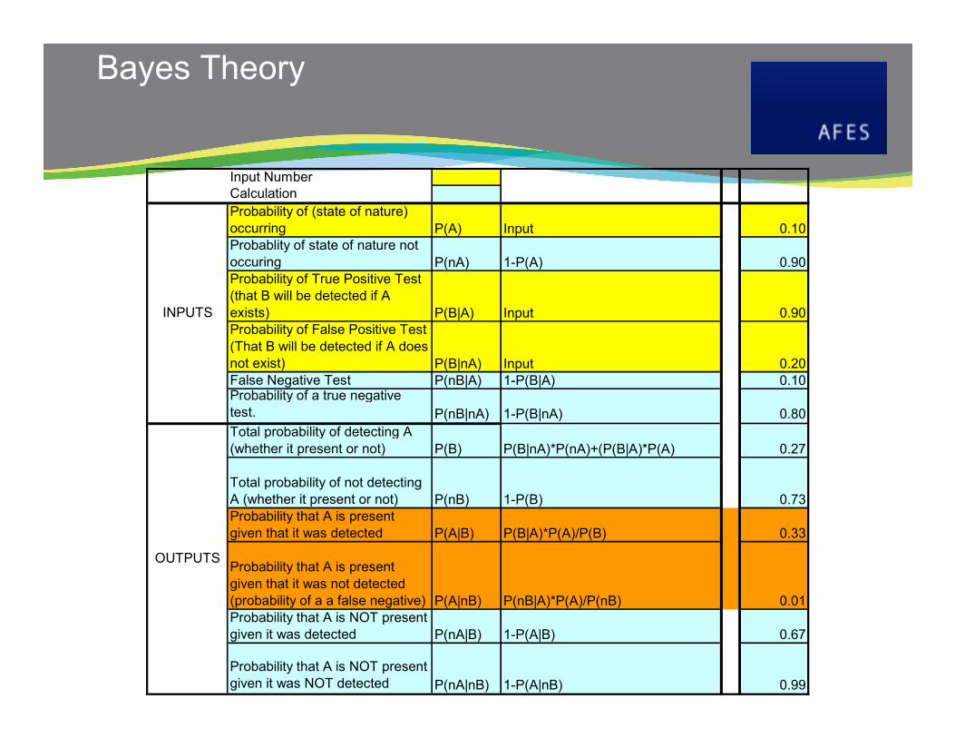
Bayes Theory

Input Number

Calculation

Probability of (state of nature)

occurring P(A) Input 0.10

Probablity of state of nature not

occuring P(nA) 1-P(A) 0.90

Probability of True Positive Test

(that B will be detected if A

exists) P(B|A) Input 0.90

Probability of False Positive Test

(That B will be detected if A does

not exist) P(B|nA) Input 0.20

False Negative Test P(nB|A) 1-P(B|A) 0.10Probability of a true negative

test. P(nB|nA) 1-P(B|nA) 0.80

Total probability of detecting A

(whether it present or not) P(B) P(B|nA)*P(nA)+(P(B|A)*P(A) 0.27

Total probability of not detecting

A (whether it present or not) P(nB) 1-P(B) 0.73

Probability that A is present

given that it was detected P(A|B) P(B|A)*P(A)/P(B) 0.33


given that it was not detected

(probability of a a false negative) P(A|nB) P(nB|A)*P(A)/P(nB) 0.01

Probability that A is NOT present

given it was detected P(nA|B) 1-P(A|B) 0.67


given it was NOT detected P(nA|nB) 1-P(A|nB) 0.99

INPUTS

OUTPUTS

Using AVO to De-risk Explorationand The Impact of Diagnosis Reliability

• AVO Anomaly

• Information

• Our geophysicist has evaluated AVO anomalies and has

assessed that:

• There is a 10% chance of geological success

• There is a 90% chance of seeing an AVO if there is a discovery

• There is a 20% chance of seeing a false anomaly if there is no

discovery

• Question

• If we have a 10% COS based on the geological interpretation

and an anomaly is observed, what is the revised COS if an

AVO is observed

• What is the added value of AVO

AVO

Geologocal COS

1 Discovery

1.1 Anomaly 9%90%

1.2 No Anomaly 1%10%

10%

2 No Discovery

2.1 Anomaly 18%20%

2.2 No Anomaly 72%80%

90%

AVO-Bayes Theory

Input Number

Calculation

Probability of (state of nature)

occurring P(A) Input 0.10

Probablity of state of nature not

occuring P(nA) 1-P(A) 0.90

Probability of True Positive Test

(that B will be detected if A

exists) P(B|A) Input 0.90

Probability of False Positive Test

(That B will be detected if A does

not exist) P(B|nA) Input 0.20

False Negative Test P(nB|A) 1-P(B|A) 0.10Probability of a true negative

test. P(nB|nA) 1-P(B|nA) 0.80

Total probability of detecting A

(whether it present or not) P(B) P(B|nA)*P(nA)+(P(B|A)*P(A) 0.27

Total probability of not detecting

A (whether it present or not) P(nB) 1-P(B) 0.73


given that it was detected P(A|B) P(B|A)*P(A)/P(B) 0.33


given that it was not detected

(probability of a a false negative) P(A|nB) P(nB|A)*P(A)/P(nB) 0.01


given it was detected P(nA|B) 1-P(A|B) 0.67


given it was NOT detected P(nA|nB) 1-P(A|nB) 0.99

INPUTS

OUTPUTS

AVO

• AVO Anomaly

• Question

• If we have a 10% COS based on the geological interpretation

and an anomaly is observed, what is the revised COS if an

AVO is observed

• What is the added value of AVO

• Answer based on Bayes is that if there is an AVO anomaly

there is a 33% chance it is a discovery.

• Also we can calculate, if there in NO AVO anomaly then the

chance it is a discovery is 1%/

Assessing Critical Porosity inShallow Hole Sections

• Synopsis of SPE paper in press

• New technique for deriving porosity from sonic logs in

oversize boreholes

• Sonic porosity used to determine of porosity is at critical

porosity

• Critical porosity 42 to 45 p.u.

• If lower than critical porosity rock is load bearing

• Near or at critical porosity the rocks may have insufficient

strength to contain the forces of shutting in the well

• Sonic porosity (using the new technique) is used to

determine if rock is below critical porosity and used as part

of the justification for NOT running a conductor

Case Study: Assessing Critical Porosity inShallow Hole Sections

• LWD acoustic compression slowness below the drive pipe

• LWD sonic device optimised for large bore holes

• Data showed conclusive evidence of absence of hazards and

were immediately accepted as waiver for running the diverter

and conductor string of casing

• DTCO used to asses if rock consolidated (below critical

porosity)

• Gives the resultant DTCO and porosity interpretation

• Raymer Hunt Gardner model with shale correction

• No mention of the reliability of the interpretation

• Processed DTCO accuracy

• Interpretation model uncertainty

Assessing Critical Porosity inShallow Hole Sections

• Question

• What is the potential impact of tool accuracy and model

uncertainty on the interpretation

• Should this be considered as part of the risk management

for making the decision on running the conductor

• What is the reliability of the method and measurement

for preventing the unnecessary running of diverter and

conductor string of casing

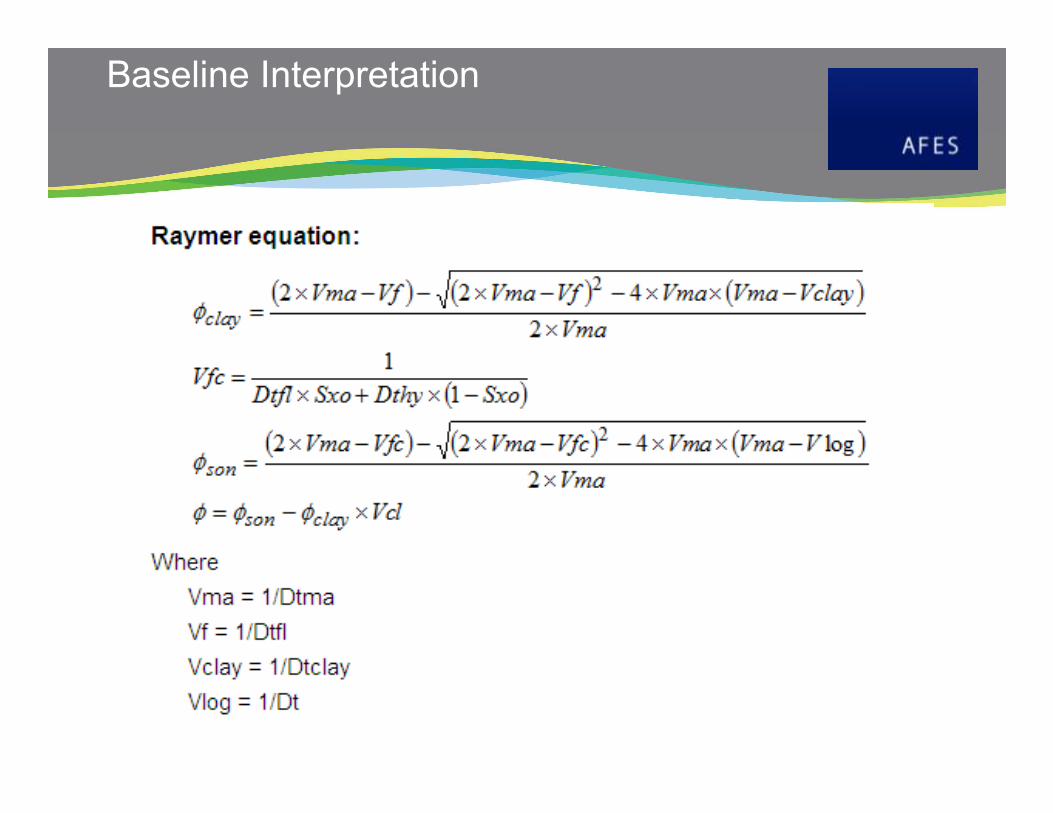
Baseline Interpretation

Baseline Interpretation

• DT matrix = 55.5 usec/ft

• DT Fluid = 189 usec/ft

• DT wet clay = 160 usec/ft

• (uncompacted sediment)

• VCL from GR using linear method

BigSonicScale : 1 : 500

DEPTH (999.89FT - 1500.37FT) 09/01/2010 15:16DB : Test (-1)

1

GR (GAPI)0. 150.

2

DEPTH(FT)

3

DTCO (usec/ft)300. 100.

4

PHIT (Dec)0.5 0.

1000

1100

1200

1300

1400

15001

GR (GAPI)0. 150.

2

DEPTH(FT)

3


4

PHIT (Dec)0.5 0.

Rock above CP

BigSonicScale : 1 : 500

DEPTH (999.89FT - 1500.37FT) 10/09/2010 10:47DB : Test (1)

1

GR (GAPI)0. 150.

2

DEPTH(FT)

3


4

PHIT (Dec)0.5 0.

ResFlag ()0. 10.

1000

1100

1200

1300

1400

15001

GR (GAPI)0. 150.

2

DEPTH(FT)

3


4

PHIT (Dec)0.5 0.

ResFlag ()0. 10.

Phi Cut Res Cutoff Sensitivity Data

Wells: BigSonic

Net Reservoir - All Zones��

Phi Cut Res Cutoff

0.40.30.20.1

Net R

eserv

oir

300

250

200

150

100

50

P10P50P90

Uncertainty Analysis (Monte Carlo)

Distribution Default + -

DTCO (usec/ft) Gaussian log 5 5

GR clean Gaussian 17 10 10

GR Clay Gaussian 84 10 10

DT wet clay (usec/ft) Gaussian 159 5 5

DT Matrix (usec/ft) Gaussian 55.5 5 5

DT Water (usec/ft) Gaussian 189 5 5

Cutoff for critical

Porosity (v/v) Square 0.42 0.03 0.01

Uncertainty Analysis (Monte Carlo)

• Footage where porosity exceeds critical porosity

• Gross Section =

• P10 = 0ft

• P50 = 23 ft

• P90 = 62.5 ft

MONTE CARLO RESULTS HISTOGRAMSBigSonic

Number of Simulation : 2000Net Res Zone : All

Mean : 29.01 Std Dev : 25.93

0

50

100

150

200

250

300

-10 110

MONTE CARLO TORNADO PLOTBigSonic

Error Analysis for : Net Reservoir

Sonic Wet Clay

DTCO

Sonic matrix

Sonic water

Gr Clay

Phi Cut Res/Pay

Gr Clean

5 159 5

5 5

5 55.5 5

5 189 5

10 84 10

0.03 0.42 0.01

10 17 10

ShiftLow

InitialValues

ShiftHigh

12.207-57.575 81.988

Net Reservoir Zone : 1

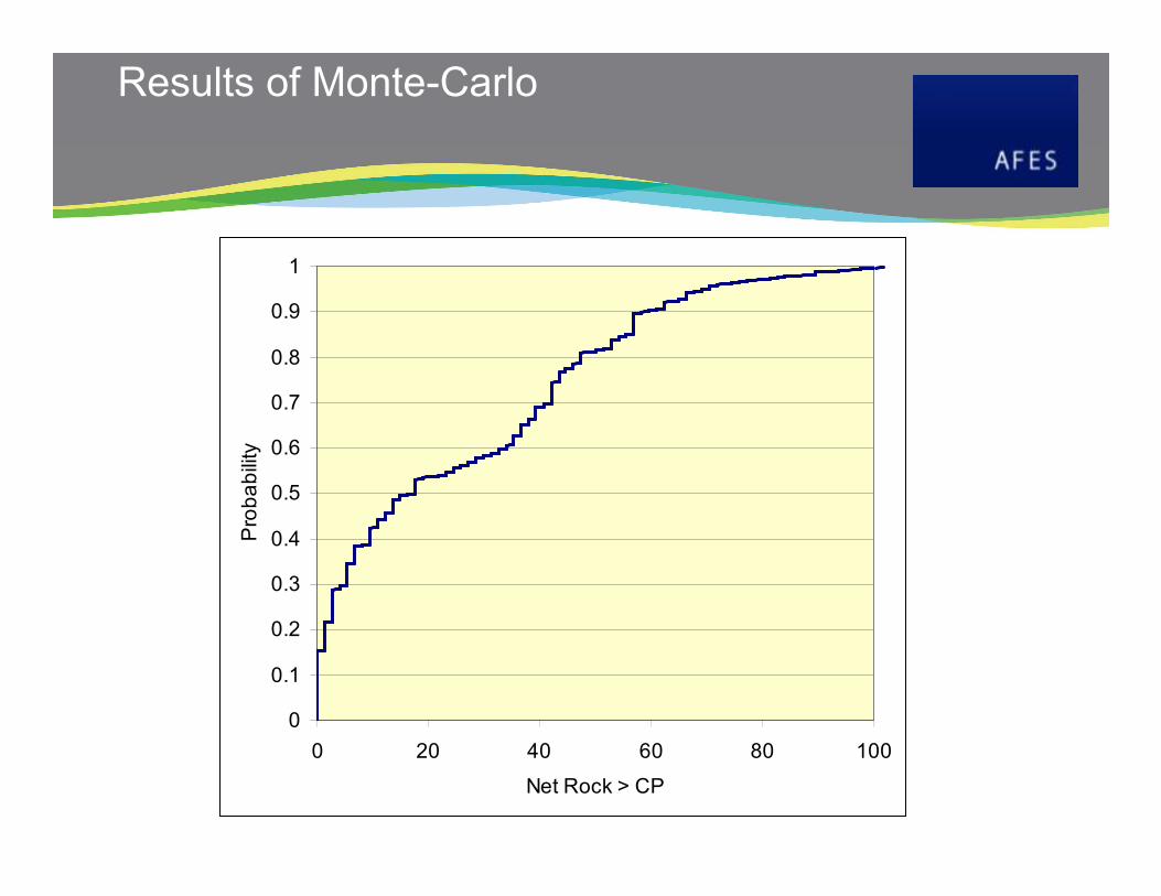
Results of Monte-Carlo

0

0.1

0.2

0.3

0.4

0.5

0.6

0.7

0.8

0.9

1

0 20 40 60 80 100

Net Rock > CP

Pro

ba

bili

ty

Tornado Plot

MONTE CARLO TORNADO PLOTBigSonic

Error Analysis for : Net Reservoir

Sonic Wet Clay

DTCO

Sonic matrix

Sonic water

Gr Clay

Phi Cut Res/Pay

Gr Clean

5 159 5

5 5

5 55.5 5

5 189 5

10 84 10

0.03 0.42 0.01

10 17 10

ShiftLow

InitialValues

ShiftHigh

12.207-57.575 81.988

Net Reservoir Zone : 1

Conclusions from Monte Carlo

• The model processed DTCO and model uncertainty leads

to significant doubt that the rock is below critical porosity

• The most important considerations are:

• The clay volume and clay correction

• The actual porosity value for critical porosity (0.41 to 0.45)

• Tool Accuracy is not a concern (+/- 5 usec/ft)

• A good question to ask is what is the tool accuracy given the

new processing technique and challenges of running sonic

in big bore-holes?

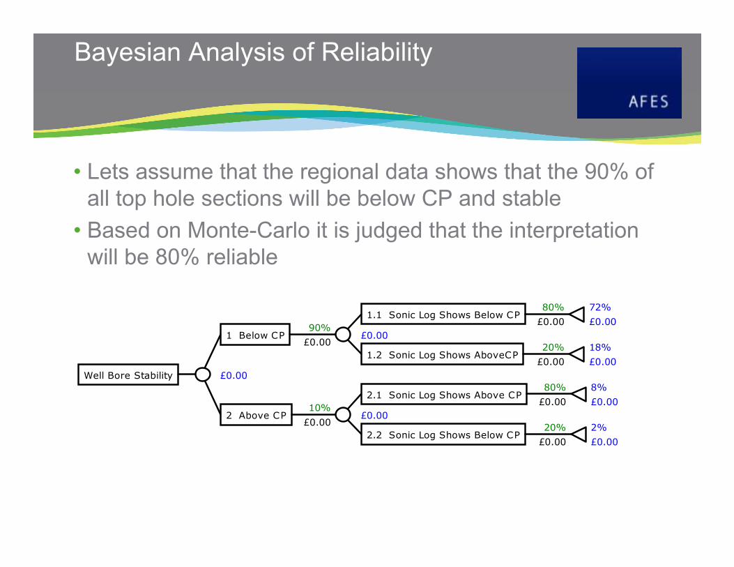
Bayesian Analysis of Reliability

• Lets assume that the regional data shows that the 90% of

all top hole sections will be below CP and stable

• Based on Monte-Carlo it is judged that the interpretation

will be 80% reliable

Well Bore Stability

1 Below CP

1.1 Sonic Log Shows Below CP72%

£0.00

80%

£0.00

1.2 Sonic Log Shows AboveCP18%

£0.00

20%

£0.00

£0.0090%

£0.00

2 Above CP

2.1 Sonic Log Shows Above CP8%

£0.00

80%

£0.00

2.2 Sonic Log Shows Below CP2%

£0.00

20%

£0.00

£0.0010%

£0.00

£0.00

Bayesian Inversion of Tree

Critical Porosity

1 Log Shows "BCP"

1.1 BCP (0.72/0.74) 72%97%

1.2 ACP (0.02/0.74) 2%3%

74%

2 LOG Shows "ACP"

2.1 BCP (0.18/0.26) 18%69%

2.2 ACP (0.08/0.26) 8%31%

26%

% Wells below CP regionally 0.9

Reliability of the log 0.8

"BCP" "ACP"

BCP 0.72 0.18

ACP 0.02 0.08

0.74 0.26

If Log shows BCP 0.97

If Log Shows ACP 0.31

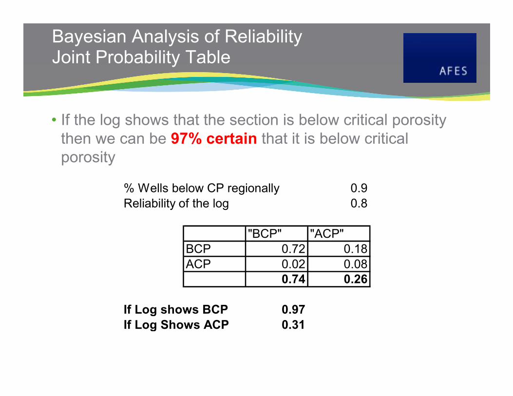
Bayesian Analysis of ReliabilityJoint Probability Table

• If the log shows that the section is below critical porosity

then we can be 97% certain that it is below critical

porosity



"BCP" "ACP"

BCP 0.72 0.18

ACP 0.02 0.08

0.74 0.26



Bayesian Analysis 2

• What if only 60% of the wells in the area are below critical

porosity. What is the value of the sonic?

• If the sonic log shows below CP there is an 86% chance it

is really below CP



"BCP" "ACP"

BCP 0.48 0.12

ACP 0.08 0.32

0.56 0.44



Reliability of Diagnosis Chart

0.00

0.20

0.40

0.60

0.80

1.00

1.20

0.5 0.6 0.7 0.8 0.9 1

Log Diagnostic Reliability

Pro

ba

bilit

y th

at

Inte

rva

l is

Belo

w C

P

0.2

0.4

0.6

0.8

1

Regional Data

% of well above

Below Cp

Conclusions From Reliability Analysis

• If the Sonic is 100% reliable as a diagnosis of the well

being above or below CP then the log data then we can be

sure the interval is above/below CP

• If the Sonic log is not 100% reliable then we need to take

into account

• Regional data trends

• Reliability of the Sonic log

• If we believe that the sonic log is less than 100%

diagnostic then there is always a risk that the well will be

above CP, even if the log data shows otherwise.

Conclusions

• The most important task of the geoscientist is to make statements about

• Range of possible subsurface outcomes based on:

• Uncertainty

• Diagnostic reliability of data

• There are several ways to analyse the range of outcomes based onuncertain input parameters

• Single parameter sensitivity

• Partial derivative analysis

• Monte-Carlo simulation

• Bayes’ analysis for diagnostic reliability

• The results of uncertainty and reliability analysis can be counter intuitive

From Monte Carlo to Bayes Theory: The Role of Uncertainty ... Bayes To Monte_Carlo AFES.pdf · From...

Documents

Transcript of From Monte Carlo to Bayes Theory: The Role of Uncertainty ... Bayes To Monte_Carlo AFES.pdf · From...