From mine to coast: transport infrastructure and the

direction of trade in developing countries

Roberto Bonfatti

University of Nottingham

Steven Poelhekke

VU University Amsterdam, Tinbergen Institute, and De Nederlandsche Bank ∗

March 11, 2013

Abstract

Mine-related transport infrastructure specializes in connecting mines to the coast, and

not so much to neighboring countries. This is most clearly seen in developing countries,

whose transport infrastructure was originally designed to facilitate the export of natural

resources in colonial times. We provide first econometric evidence that mine-to-coast trans-

port infrastructure matters for the pattern of trade of developing countries, and can help

explaining their low level of regional integration. The main idea is that, to the extent that

it can be used not just to export natural resources but also to trade other commodities, this

infrastructure may bias a country’s structure of transport costs in favor of overseas trade,

and to the detriment of regional trade. We investigate this potential bias in the context

∗Views expressed are those of the authors and do not necessarily reflect official positions of De NederlandscheBank nor of the Eurosystem of central banks. We are grateful to Brian Kovak, Torfinn Harding, Pierre-LouisVezina, Tony Venables, seminar participants at the University of Oxford, VU University Amsterdam, the EBRD,the 2011 CSAE Conference in Oxford, the 2012 Rocky Mountain Empirical Trade Conference in Vancouver, andthe 2012 ETSG for helpful comments and suggestions.Both authors are also affiliated with OxCarre and CESIfo.

1

of a gravity model of trade. Our main findings are that coastal countries with more mines

import less than average from their neighbors, and this effect is stronger when the mines

are located in such a way that the related infrastructure has a stronger potential to affect

trade costs. Consistently with the idea that this effect is due to mine-to-coast infrastruc-

ture, landlocked countries with more mines import less than average from their non-transit

neighbors, but more then average from their transit neighbors. Furthermore, this effect is

specific to mines and not to oil and gas fields, arguably because pipelines cannot possibly

be used to trade other commodities. We discuss the potential welfare implications of our

results, and relate these to the debate on the economic legacy of colonialism for developing

countries.

JEL Codes: F14, F54, Q32, R4.

Keywords: Mineral Resources, Transport Infrastructure, Regional Trade Integration,

Gravity Model, Economic Legacy of Colonialism.

1 Introduction

The economic legacy of colonialism has attracted renewed attention in recent years, as a number

of empirical papers have sought to test various theoretical arguments about the effect of colonial

policies on contemporary economic performance (for two recent contributions, see Feyrer and

Sacerdote, 2009, and Iyer, 2010). One argument that has received little attention by modern

economists, but that was hugely influential in the past, holds colonial policies responsible for

destroying local and regional trade in the colonies, to the benefit of trade between the colonies

and the colonizer. In the long-run, the argument goes, this led to an adverse pattern of special-

ization, whereby all high value-added activities are undertaken overseas, and the former colonies

are bound to a condition of dependency on their former colonial masters (e.g. Dos Santos, 1970;

Amin, 1972). Key to this result, it is claimed, was investment in transport infrastructure. Colo-

nial rails and roads were constructed to connect the interior to the coast; they were intended to

facilitate the export of raw materials and the import of European manufactures, and had nothing

2

to do with the needs of local and regional trade (e.g. Rodney, 1982, p. 209).1 By strengthening

the comparative advantage of overseas manufactures, this infrastructure contributed to displac-

ing existing local and regional producers. Colonial transport infrastructure has persisted over

time, contributing to explain the former colonies’ little regional integration and disappointing

economic performance after decolonization.

A casual look at a map of colonial transport infrastructure immediately illustrates why this

argument may have gained considerable popularity. Map 1 in Appendix A describes West and

East African railways in the 1960s, the years following independence. The map clearly shows

that colonial railways mostly connected the interior to the coast, while there were very few links

connecting neighboring countries; furthermore, many of the latter links were designed primarily

to connect the interior of a landlocked country to the coast. Strikingly, this pattern seems

to have remained unaltered in the thirty years following independence. Map 2 describes the

structure of African railways in the 1990s, which appears to be very similar to those in the

previous map. In Appendix B, we provide a case study of Ghana, a resource-rich country where

the colonial transport infrastructure had a clear interior-to-coast pattern, and has persisted after

decolonization.

While an interior-to-coast pattern of transport infrastructure does not per se allow us to

conclude that such infrastructure is sub-optimal, such a conclusion actually permeates the con-

temporary trade and development literature. For example, the trade literature has repeatedly

documented the fact that intra-African trade is “too small” compared to what the gravity model

of trade predicts, and that much of it can be attributed to the poor quality of transport infras-

tructure (e.g. Limao and Venables, 2001).2 Sachs et al. (2004, p. 182) explicitly blame this

on interior-to-coast transport infrastructure: “Not only does sub-Saharan Africa have extremely

low per capita densities of rail and road infrastructure, but indeed existing transport systems

were largely designed under colonial rule to transport natural resources from the interior to the

nearest port. As a result, cross-country transport connections within Africa tend to be extremely

1A second key rationale of colonial investment in infrastructure was to facilitate the establishment of militaryand political control over the interior.

2This is quite evident in the raw data: African countries were less than half as likely to import from neighborsthan the average OECD country in 2006, and imported only a quarter of all their imports from other Africancountries (see Table 1 in Appendix D).

3

poor and are in urgent need of extension, to reduce intraregional transport costs and promote

cross-border trade”. The African Development Bank has recently taken up this challenge, by

drafting an ambitious plan to improve the overland connections between Sub-Saharan African

countries (Buys et al., 2006).3

In this paper, we provide first econometric evidence that the current small volumes of regional

trade in developing countries may be attributed to their specialization in the export of natural

resources, and the related stock of interior-to-coast transport infrastructure. In particular, we

focus on the impact of mine-to-coast infrastructure. Drawing inspiration from some of the ar-

guments of dependency theorists, we formulate and test the following hypothesis. International

specialization implies that developing countries tend to export their mineral resources to devel-

oped countries. Because developed countries are mostly located in overseas continents from the

perspective of developing countries, such exports will require the construction of transport infras-

tructure connecting mineral-rich regions of the interior to the coast, and from there to overseas

markets. Thus, we expect that developing countries with a larger number of active mines will

have a larger and better stock of transport infrastructure (rail, roads, and ports) connecting their

mines to the coast. To the extent that such infrastructure can also be used to import a broad set

of goods, it will reduce the transport costs on import from overseas countries disproportionately

more than on imports from regional trading partners. Furthermore, if such infrastructure has

dominated national infrastructural investment (because of the long-run effect of colonial policies,

or because of other reasons that we discuss below), these countries’ overall structure of transport

costs will also be biased in favor of imports from overseas countries. Thus, we expect that, on

average, a larger number of active mines should result in “trade re-direction effect” in developing

countries, favoring imports from overseas countries to the detriment of imports from regional

trading partners.

We build our empirical strategy on the following steps. We begin by estimating a gravity

model of bilateral trade flows (controlling for importer and exporter fixed effects and a range of

measures of trade costs) to show that, indeed, countries with more mines import less than average

3The authors estimate that the realization of such a plan would expand overland trade by about $250 billionover 15 years, greatly outweighing the cost of initial upgrading and annual maintainance.

4

from regional trading partners, here simply defined as countries with which the destination

country shares a border. This qualifies the standard gravity result that neighboring countries

trade more with each other, and may eliminate it or even overturn it for countries that have

a sufficiently larger number of mines.4 When we split the sample in OECD vs non-OECD

destinations, we find that this trade re-direction effect disappears for the first group of countries,

while it is still there for the second group of countries. This is prima-facie evidence in favor of our

hypothesis, since we would have expected a larger number of mines to have a trade re-direction

effect in developing countries, and in developing countries only.5

While we would like to test directly whether or not this trade re-direction effect of mines

can be attributed to the existence of mine-to-coast transport infrastructure, lack of data on the

size, quality and direction of transport infrastructure for a sufficiently large number of countries

prevents us from following that approach. We therefore use a number of strategies to test our

hypothesis indirectly.

First, our hypothesis predicts that the trade re-direction effect should be stronger when the

(exogenous) location of mines is such that the related transport infrastructure has a stronger

impact on trade costs. For example, imagine to draw a straight line connecting a mine to the

closest point on the coast. If this line cuts through many cities, we expect the mine-to-coast

transport infrastructure associated with the mine to have a large potential for trade re-direction,

since its presence will affect the transport costs faced by a large proportion of the country’s

population. We construct an index capturing the ‘trade re-direction potential’ of a country’s

mines, and test for the prediction that, for a given number of mines, the trade re-direction effect

is stronger in countries with a higher value of the index.

The second strategy derives from the existence of landlocked countries in our sample. Devel-

oping, landlocked countries will also tend to export most of their mineral resources to overseas

countries. However, for these countries the mine-to-coast transport infrastructure will necessarily

4For example, we find that the positive neighbor effect on trade disappears altogether for the 40 most importantmining countries.

5Developed countries will tend to retain a larger part of their mineral resources for domestic or regionalconsumption, and a larger number of mines will then be less likely to result in a network of transport infrastructurethat is more biased in favor of overseas trade. Moreover, it is only in developing countries that the negative long-run impact of colonial investment should be apparent.

5

cut through at least one “transit” neighbor. If mine-to-coast transport infrastructure is what is

driving the trade re-direction effect, such effect should disappear for imports from transit neigh-

bors. This is because these countries benefit from the mine-to-coast transport infrastructure just

as much as overseas countries do, if not more. We thus adopt a specification where we distinguish

between transit and “normal” neighbors , and test for any difference in the trade re-direction

effect between the two. We also expect that mines should only have a systematically different

impact on imports from transit neighbors (relative to normal neighbors) in non-OECD countries,

but not in OECD countries.

Finally, our last strategy is a falsification exercise. This is based on the observation that, if

mine-to-coast transport infrastructure is what is driving the trade re-direction effect of mines,

this effect should disappear when we look at specific types of mineral resources that are unlikely

to generate infrastructure that can be used by other trades as well. We therefore add the number

of oil and gas fields to our main specification, on the premise that oil and gas, differently from

other mineral resources, are mostly transported through pipelines.

We find compelling evidence in favor of our hypothesis. First, for a given number of mines

in the destination country, we find that the trade re-direction effect is larger when the index

measuring the trade re-direction potential of the country’s mines is higher. In other words, the

exogenous location of mines has an independent effect on the direction of national trade, and this

is consistent with the existence of mine-to-coast transport infrastructure associated with those

mines. While this effect is non significant for non-OECD destinations, it is highly significant in

a subset of all African destinations. Next, we find that landlocked destination countries with

a larger number of mines import less the average from their normal neighbors, but more than

average from their transit neighbors. As expected, this effect holds only for (less developed)

non-OECD countries. Finally, our falsification exercise yields the desired result: there is no

trade re-direction effect associated with the number of oil and gas fields nor their location, and

this results extends to all of our subsamples.

These results are consistent with the idea that specialization in the export of natural resources

has, through transport infrastructure, a trade re-direction effect that penalizes regional trade.

One must be very careful in drawing quick welfare implications from these results, however.

6

For one thing, even if the interior-to-port transport infrastructure is biased in favor of imports

from overseas countries, it will still decreases overall national transport costs. Since this will

have positive welfare implications for domestic consumers and producers, we cannot draw any

clear welfare implications for the country where the interior-to-coast transport infrastructure is

built. Furthermore, we cannot conclude that developing countries with more mines trade less

with neighbors in absolute terms. This is because all of our specifications include importer fixed

effects, which will absorb any positive (or negative) effect that the mines have on national trade.

Still, our results allow us to make some interesting conjectures on possible welfare implica-

tions. The interior-to-coast transport infrastructure is likely to have a negative welfare effect on

local and regional industries that compete with imports from overseas countries. For these in-

dustries, such infrastructure may entail a substantial reduction in market access, which may lead

to severe efficiency losses (e.g. Collier and Venables, 2010). More in general, the segmentation

of regional markets may lead to a suboptimal size of regional centers of production (e.g. cities),

and thus to an overall fall in productivity (ibid.). Such small-market effects are often thought to

be consequential for the capacity of developing countries to achieve economic growth (e.g. Sachs

et al., 2004, p. 131). Clearly, we expect these effects to be particularly negative for regional

trading partners, since these countries do not benefit from a direct reduction in transport costs.

The paper is organized as follows. The next section discusses the related literature, after

which we construct a simple gravity model that illustrates our idea and derives our hypothesis

in sections 3 and 4. After describing the data in section 5, we test our hypothesis in section 6.

We then use section 7 to discuss welfare implications, and section 8 to conclude.

2 Related literature

The paper is related to a growing literature on the impact of infrastructure on economic perfor-

mance. A first group of papers have studied the long-term impact of infrastructure. For example,

Banerjee et al. (2012) find that Chinese areas that were “treated” with a railway connection

in late 19th century were somewhat richer in 1986, but did not benefit disproportionately from

subsequent Chinese growth. Faber (2012) finds the construction of highways in China favored the

7

concentration of industrial activity in larger locations, to the detriment of smaller ones. Jedwab

and Moradi (2012) focus on the long-term impact of colonial railways in Ghana, finding that

places that were connected by the railway are more developed today. A second group of pa-

pers have focused on the impact of infrastructure on market integration and welfare. Donaldson

(2012) finds that colonial railroads in India had a major impact on trade integration between

Indian regions and with the rest of the world, implying a positive welfare effect. Keller and Shiue

(2008) find that railways had a stronger market integration effect on 19th century Europe than

custom liberalizations and monetary unions.6 We contribute to this literature by investigating

the asymmetric market integration effect of transport infrastructure. Furthermore, while the

above-mentioned literature focuses on exogenous variation in the placement of infrastructure, we

explicitly test a hypothesis that relates the placement of infrastructure to a country’s natural

resources.

The idea that a country’s natural resource production may adversely bias national trade

patterns dates back to the so-called “Dependency School”. This held that integration in the world

economy has put developing countries in a position of dependency, whereby, by specializing in

the export of primary products and becoming dependent on the world economy for imports of all

other products, they fall in a condition of underdevelopment. This process was facilitated by the

colonial and neo-colonial relation that these countries entertained with some of the key players

in the world economy. This thesis took its origins in the famous work on developing countries’

terms of trade by Prebisch (1950) and Singer (1950), and became very influential in the 1960s and

1970s as an antithesis to modernization theories.7 The argument that transport infrastructure

played a key role in all this has been made, among others, by Rodney (1982, p. 209), and

Freund (1998). For example, Rodney states that “The combination of being oppressed, being

exploited, and being disregarded is best illustrated by the pattern of the economic infrastructure

of African colonies: notably, their roads and railways. These had a clear geographical distribution

according to the extent to which particular regions needed to be opened up to import-export

activities. [...] There were no roads connecting different colonies and different parts of the same

6A third paper in this literature is Michaels (2008). The paper looks at the labor market effect of a decreasein trade costs within the US, as brought about by highway construction in the 1950s.

7See Dos Santos (1970) and Amin (1972) for details.

8

colony in a manner that made sense with regard to Africa’s needs and development. All roads

and railways led down to the sea. They were built to extract gold or manganese or coffee or

cotton. They were built to make business possible for the timber companies trading companies,

and agricultural concessions firms, and for white settlers. Any catering to African interests was

purely coincidental.”However, to the best of our knowledge, no other paper has systematically

tested this with data on mines.

Our paper looks for evidence that developing countries’ transport infrastructure - much of

which was inherited from colonial times - biases this country’s structure of international trade

against regional integration. Because of this, the paper is related to the literature on the eco-

nomic legacy of colonial empires. This has been very prolific in recent years, after the seminal

paper by Acemoglu et al. (2001) argued that much of today’s comparative development can be

explained with different institutional investments made by colonizers in different colonies. Recent

contributions include Nunn (2008), on the long-run consequences of the slave trade on Africa;

Huillery (2009), on the long-run effects of public investment in colonial French Africa; and Iyier

(2010) on the comparative long-run impact of direct versus indirect colonial rule in India. We

contribute to this literature by looking at the long-run effect of colonial investment in infras-

tructure. Although Huilery (2009) and the above-mentioned studies by Banerjee et al. (2012)

and Jedwab and Morady (2012) also look at this, we test for a specific hypothesis regarding the

negative impact of colonial infrastructure on contemporary regional trade.

The literature on the pattern of intra-African trade has investigated the openness to trade of

African countries among each other, relative to the standard provided by the gravity equation.

For example, Limao and Venables (2001) find that trade between pairs of Sub-Saharan African

(SSA) countries is significantly lower than trade between pairs of non SSA countries, even after

controlling for income, per capita income, neighbors and other standard geographical variables

such as distance and an island dummy. However after controlling for a rough measure of national

infrastructure,8 this difference becomes significantly positive. They also find that the negative

effect of distance on bilateral trade flows is larger for SSA than for non-SSA pairs.

8The authors use Canning (1998)’s index of road, paved road and railway densities and telephone lines percapita.

9

In our mechanism, the need to export natural resources leads to a biased structure of transport

costs in developing countries, which favors trade with overseas trading partners to the detriment

of trade with regional trading partners. Because a fall in transport costs has a similar effect

on trade patterns as a fall in tariffs, our mechanism is conceptually related to the literature on

North-South vs South-South trade agreements (or custom unions). Such literature has sought to

understand whether the interests of developing countries in the South are better served by trade

agreements with developed countries in the North, or with neighboring developing countries. For

example, Venables (2003) finds that for a medium-income developing country, to sign a custom

union with developed countries may be less welfare-enhancing than to sign it with a low-income

neighbor, while for the latter the opposite is likely to be true.

The literature on the resource curse (see van der Ploeg, 2011, for a recent survey) has pre-

sented various arguments why natural resource booms may not be a great source of domestic

growth for developing countries. Our results suggest that they may not be a great source of

growth for regional trading partners either, if they are accompanied by an infrastructure-driven

re-orientation of trade towards overseas countries. Because of these implications, the paper

is related to the literature on international growth spillovers (e.g. Easterly and Levine, 1998;

Roberts and Deichman, 2009), and particularly those papers that look at natural resource booms

explicitly (e.g. Venables, 2009).

3 Model

We begin from a standard gravity equation specifying the expected imports of country d (“des-

tination”) from country o (“origin”):

ln impod = k − ln τ̃od + ao + ad + vod, (1)

where k is a constant, τ̃od is an index capturing all costs incurred to import goods from o to

d, ao and ad are origin and destination fixed effects, and vod is a random error. Our goal is to

determine how τ̃od will depend on the number of mines in d, for all possible o.

10

Consider first a world with a number of separate continents, but only coastal countries. A

stylized image of such a world is represented in Figure 4, Panel I (Appendix C), which represents

a destination country and n origin countries (oi), both on the same continent as d (i = 1, ..., 5)

and on separate continents or “overseas” (i = 6, ..., n). Overseas origin countries are connected

to the destination country through a sea route, terminating at port P . The existence of mines in

the destination country will normally be associated with the existence of mine-related transport

infrastructure, some of which will be connecting the mines to foreign markets. In the figure, the

potential location of such infrastructure is represented by all the lines that connect mine M to

foreign countries.

Assume that the mine-related transport infrastructure connecting d to some oi is usable by

other trades as well, thus reducing d’s cost of importing from oi. The question then arises: on

average, will this favor imports from all oi in a roughly similar manner, or will it be systematically

biased in favor of some oi?

Assume that d is a developing country from now on. Developing countries export most of their

natural resources to industrialized countries, and these are located overseas from the perspective

of most developing countries. It follows that we expect d’s mine-related infrastructure to be more

likely to connect point M to point P - from where the natural resources can be shipped overseas

- than to neighboring countries. In other words, we expect d’s mine-related infrastructure to be

likely to have a “mine-to-coast” trajectory. In Figure 4, this is represented by the fact that the

line connecting M to P is thicker than the lines connecting M to neighboring countries.9

To the extent that d’s imports from neighbors are less likely to be routed through P than

imports from non-neighbors, one hypothesis that we may then put forward is that the mine-

related transport infrastructure will be more likely to reduce transport costs on import from

i = 6, ..., n than on imports from i = 1, ..., 5. Because the same logic applies to each mine

existing in d, we expect this effect of mine-related transport infrastructure to be stronger, the

larger is the number of mines in d (the more points M there are).

9Developing countries have also largely inherited their transport infrastructure from colonial times. Sincecolonizers were primarily interested in the export of natural resources, the mine-to-coast transport infrastructureis likely to dominate these countries’ transportation system, resulting in the asymmetric pattern illustrated inFigure 4

11

Denote by φ6N the probability that the mine-related infrastructure connects point M to point

P (that is, it has a mine-to-coast trajectory), and by φN the probability that it connects it

to a neighboring country. We then expect that, if d is a developing country, φ6N > φN should

hold.10 Next, suppose that we are able to construct an index αd ∈ [0, 1], measuring the extent

to which the mine-to-coast transport infrastructure overlaps with the location of d’s consumers

(for example, with cities), and thus actually contributes to reducing their import costs. In the

next section, we will construct this index in such as way as to exploit the location of mines as a

source of exogenous variation. We then hypothesize that d’s cost of importing from some oi is

determined as follows:

ln τ̃od = ln τod −NodφNγMd − (1−Nod)φ6Nγ (1 + αd)Md − δNod, (2)

where Nod is a neighbor dummy, γ > 0 is a parameter that measures the extent to which,

on average, the mine-related transport infrastructure is usable by other trades as well, Md is

defined as ln(1 + md), where md is the number of active mines in d, and δ > 0 is a parameter

that allows for the fact that transport costs may be lower between neighboring countries for

reason that have nothing to do with mine-related infrastructure. The term τod is then implicitly

defined as the cost of importing from some non-neighboring oi when d has no mines (that is,

there is no point M). The second and third terms in the above expressions capture the positive

effect that the mine-related infrastructure is expected to have on d’s import costs. Provided that

d is a developing country - provided that φ6N > φN - we expect this effect to be stronger for

imports from o6, ..., on (for which Nod = 0) than for imports from o1, ..., o5 (for which Nod = 1).

Furthermore, we expect this difference to be larger, the more d’s mine-to-coast infrastructure

happen to overlap with the location of its consumers (the larger is αd).11

Next, consider a world in which there are also landlocked countries, and consider the im-

pact of mine-related transport infrastructure on a landlocked destination country. This case is

10For developed countries, we expect these two probabilities to be very small (since developed countries tendto export a smaller proportion of their natural resources) and roughly similar to each other (since developedcountries are both neighbors and non-neighbors from the perspective of many developed countries). Both factorssuggests that the difference between φ 6N and φN should be close to zero for developed countries.

11Which we later construct on the basis of the relative location of cities, ports, and mines.

12

represented in Panel II of Figure 4. As for the case of a coastal d, we expect that, if d is a

developing country, its mine-related infrastructure will be more likely to connect M to P than

to a neighboring country. From a landlocked d, however, P can only be reached by first passing

through a transit neighbor such as o3. It follows that, for a landlocked d, we still expect the

mine-related transport infrastructure to be more likely to reduce transport costs on imports from

o6, ..., on than from non-transit neighbors such as o1, o2, o4 or o5. However the two probabilities

should be roughly the same for o6, ..., on and d’s transit neighbor, o3.

To account for the existence of landlocked destination countries, we modify equation (2) as

follows:

ln τ̃od = ln τod −NodφNγMd − (1−Nod)φ6Nγ (1 + αd)Md − δNod

−NodTodLdγ(φ6N − φN

)Md −NodTodLdγφ

6NαdMd − ζTod, (3)

where Tod is a dummy that takes value 1 if and only if oi and d are in a transit relation, Ld

is a landlocked dummy for the destination country, and ζ > 0 is a parameter that captures the

fact that transport costs may be lower between countries in a transit relation, for reason that

have nothing to do with mine-related infrastructure. To interpret equation (3), consider how the

second row modifies the expression of transport costs for a landlocked d (Ld = 1). Basically, we

still expect the effect of mine-related infrastructure to be stronger for imports from o6, ..., on than

from o1, o2, o4 and o5 (for which Nod = 1, Tod = 0), but not from o3 (for which Nod = Tod = 1),

where the marginal effect of Md is the same as in the case of o6, ..., on ((1 + αd)Md).

Re-arranging equation (3) yields:

ln τ̃od = ln τod − φ6Nγ (1 + αd)Md+

+(φ6N − φN

)γMdNod + φ6NγMdNodαd − δNod−

−NodTodLd

(φ6N − φN

)γMd −NodTodLdγφ

6NαdMd − ζNodTod (4)

Having constructed an expression for the expected impact of mines on transport costs, we can

plug this back into our gravity equation, Eq. (1). Because the term φ6Nγ (1 + αd)Md captures

13

characteristics of the destination country only, we can - with a slight abuse of notation - include

it in d’s fixed effect. The gravity equation then becomes:

ln impod = k − ln τod + ao + ad+

+ β1NodMd + β2NodMdαd + β3Nod+

+ β4NodTodLdMd + β5NodTodLdMdαd + β6NodTod + vod, (5)

where β1 ≡ −(φ6N − φN

)γ, β2 ≡ −φ6Nγ, β3 ≡ δ, β4 ≡ (φ6N − φN)γ, β5 = φ6Nγ, β6 = ζ.

Equation (5) is our main theoretical equation. The variables contained in the first row of equation

(5), as well as Nod and Tod, are standard gravity variables, and we expect β3, β6 > 0: neighbors

trade more with each other, and that effect is stronger for neighbors that are also in a transit

relation.

Our coefficients of interest are β1, β2, β4, β5. Our hypothesis implies that, if we run (5) for

developing destination countries, it should be β1, β2 < 0 as long as the mine-related transport

infrastructure is such to be physically usable by other trades as well (e.g. roads or railways,

for which γ > 0). This is because a larger number of mines is associated with a better stock

of mine-related infrastructure, which in developing countries is disproportionately likely to have

a mine-to-coast trajectory. This disproportionately reduces the cost of importing goods from

overseas countries, penalizing imports from neighbors (β1 < 0). This trade re-direction effect

is stronger, the more the mine-to-coast infrastructure overlaps with the route naturally used

by domestic consumers to import from overseas countries (β2 < 0). To run (5) for developed

destination countries, or for the case in which the mine-related transport infrastructure cannot be

possible used by other trades (e.g. pipelines, for which γ = 0), should instead yield β1 = β2 = 0.

Our hypothesis also implies that, if and only if β1, β2 < 0, we should also find that β4, β5 > 0:

in the case of a landlocked destination country importing from its transit neighbor, the trade re-

direction effect of the mine-to-coast transport infrastructure should be reduced (if not completely

offset) by the fact that this infrastructure will have to cut through the transit neighbor to reach

the coast.

14

4 The impact of the location of mines on import routes

In the previous section, we have hypothesized that the mine-related infrastructure of a developing

destination country is disproportionately likely to have a mine-to-coast trajectory, and may thus

reduce import costs from overseas more than from neighbors. We now construct the mine impact

index α ∈ [0, 1], measuring the extent to which the mine-to-coast infrastructure overlaps with

the location of d’s consumers, and thus actually contributes to reducing their imports costs from

overseas. Our approach is to consider how the geographical position of mines compares to that of

cities, and how the ideal position of a port intended for the exports of mines’ products compares

to that of the country’s main container port. The index offers a stylized interpretation of all

potentially relevant geography, but this provides in our view the simplest sufficient approximation

without having to resort to a full cost-benefit analysis of all possible routes and transport modes.

Consider a generic destination country d. Denote by C the geographical center point of

cities, by M that of mines, and by P the country’s main container port. Imagine to draw a line

connecting C to P . A representation is provided in either panels of Figure 5. Next, draw the

perpendicular dropping from M to the CP segment, and call I the point where the two lines

intersect (Figure 5, panel I). Alternatively, if the perpendicular falls outside the segment CP ,

connect point M to point C (Figure 5, panel II). Finally, call S the closest coastal point to M .12

Our proposed index is:

αd = 0 if πd below average

αd = 1 if πd above average,(6)

where:

πd = Pr {mines use P} ∗ Pr {mines use CP} ∗ share of CP used by mines, (7)

12Notice that in many cases (e.g. Congo, the DRC, Kazakhstan, Zambia) point S may be in a third country.

15

and where:

Pr {mines use P} =

MS+1MP+1

if MS < MP

1 if MS > MP(8)

Pr {mines use CP} =

MP+1MI+IP+1

if IP < CP

MP+1MC+CP+1

if IP > CP(9)

share of CP used by mines =

IP+1CP+1

if IP < CP

1 if IP > CP.(10)

Equations (6)-(10) suggests that our mine impact index is a discrete version of a continuous

mine-impact index index πd. The latter is the product of three distinct terms. The first term is

the probability that the mines use P to export their products, as opposed to the ideal, purpose-

built port. Because P is the country’s main container port, it is logical to expect that a large

proportion of the country’s overseas imports will be shipped through this port. Thus, a logical

prerequisite for the mine-to-coast infrastructure to reduce transport costs for overseas imports is

that such infrastructure converges to P . We proxy for the probability that this happens through

the expression in equation (8), whose logic is explained in either panel of Figure 5.13 Basically,

mine-owners face a choice between exporting the resources through P , or establishing a purpose-

built port somewhere else along the country’s coast. We assume that the ideal location for such

a port is S, that is the closest coastal point to M . Mine-owners only base their choice on the

relative distance of P and S: the closer is P relative to S, the higher is the probability that they

choose P . At the two extremes, if M is on the coast (M = S) and P is infinitely far, mine-owners

always chooe S; if P is actually the closest coastal point to M (P = S), mine-owners always

choose P .

The second term is the probability that the mines use a route overlapping with CP to reach

P , as opposed to a more direct route. Since CP is the most direct route between the cities and P ,

it is logical to expect that a large proportion of the country’s overseas imports will be channelled

through this route. Thus, a pre-requisite for the mine-to-coast infrastructure to reduce transport

costs for overseas imports is that such infrastructures overlaps with CP . We proxy for the

13Notice that, as required of a probability, this expression takes value between 0 and 1.

16

probability that this happens by the expression in equation (9), whose logic is also illustrated

in Figure 5. Having decided to ship their resources through P , mine-owners face the choice of

whether to use, at least partially, the connection CP , or rather use a more direct route such as

MP . As for the choice between P and S, mine-owners make a distance-based decision. However,

we now need to distinguish two cases. When M is located as in the first panel of Figure 5, mine-

owners compare the direct route MP to a route that joins CP on its closest point (segment CI)

and then continues along a portion of CP to the port (segment IP ). The first row of equation

(9) captures the outcome of the mine-owners’ choice in this case. The smaller is MI+IP relative

to MP , the higher is the probability that mine-owners carry the resources to P using, at least

in part, CP . At the two extremes, if M is located on CP (MI = 0, IP = MP ), mine owners

always use CP . If CI = IP , mine-owners use CP with a lower probability√

2∗IP+12∗IP+1

.14

The case when M is located as in the second panel of Figure 5 is treated very similarly,

except that mine-owners now compare the direct route MP to a route that joins MP at point

M (segment MC) and then continues along the whole of CP to the port. The second row

of equation (9) captures the fact that the smaller is MC + CP relative to MP , the higher the

probability that mine-owners use CP . As in the previous case, this probability is defined between

1 and√

2∗IP+12∗IP+1

.

Finally, for a given probability that the mines use port P to ship their resources, and reach

it through CP , the third term in equation (7) captures the extent to which the mine-related

infrastructure will actually improve CP . We assume such impact to be proportional to the share

of CP that the mine-related infrastructure actually overlaps with. Thus, when M is located as

in the first panel of Figure (5), the impact of the mine-related infrastructure is larger, the larger

is IP relative to CP (and ranges from 0 to 1 as I moves from P to C). When M is located as in

the second panel of Figure (5), the impact of the mine related infrastructure is always maximum

(that is, 1).

Having constructed the index πd, we then take a discrete version of it and use it as a our mine

impact index (αd). Although it is possible to work with πd directly, we found that this did not

lead to meaningful results. This probably means that our approximation is not accurate enough,

14Thus, the probability that mine-owners use CP is defined between√

2∗IP+12∗IP+1 and 1.

17

for example because it omits some other relevant feature of geography or because of variation in

the modes of transport of different goods in different countries. However, without other priors

on how to measure the true impact of the location of mines on city-port infrastructure and total

imports, we choose to split the sample into two groups: those with a ‘high’ score, and those

with a ‘low’ score of πd. The index αd is then attributed value 1 when πd is above the average,

value 0 when it is below. It is unlikely that these two groups would change composition much

by choosing a different definition of πd. For example, we indeed find that the results based on

the indicator are robust to using different metrics of point C.

We conclude this section by considering the case of landlocked countries as illustrated in

Figure 6. Denote by CT the geographical center point of cities in the transit country, and by P T

that country’s main container port. Then, we construct the index just as indicated in (6)-(10),

except that we substitute P with P T and CP with CCTP T . The latter is a hypothetical line

connecting C to P through CT .

5 Data

To estimate the effect of mine-related transport infrastructure on trade we need bilateral trade

flows between as many countries as possible, as well as a measure of mine-related transport

infrastructure. For trade, we rely on the UN Comtrade database which reports all known bilateral

trade flows between countries in the world based on the nationality of the buyer and seller.15 We

measure the value of trade at the importing country and use the 2006 cross-section, which should

cover more countries (particularly for Africa) and be of better quality than historical data. Even

for this recent year, we find that out of 49,506 (223 by 223-1) possible trade flows only 57% are

positive, while the other observations are coded as missing in Comtrade. Within Africa, there

are 55 by 54 possible trade flows, and in 2006 we observe 60% positive flows. No trade flows are

missing between OECD countries. Our typical regression will be able to include around 24,000

observations.

Our ideal explanatory variable would be a measure of mine-related transport infrastructure

15SITC Rev. 2, downloaded on Oct 30th, 2009.

18

that takes into account not only the amount of infrastructure, but also its quality and direction

(that is, whether it has a mine-to-coast trajectory or not). Although data exists on the total

length of the paved road and rail network in many countries, we cannot observe the quality and

direction of mine-related infrastructure directly. As explained in the previous section, we will

therefore use the number of active mines as a proxy for the amount and quality of mine-related

infrastructure. We will work under the identifying assumption that, in developing countries (and

in these only), mines tend to have a mine-to-coast trajectory, and that the effect of this on

transport costs will also depend on the location of mines, and on the type of resource exported.

For us to be able to estimate equation (5), we first of all need data on the number of active

mines in each country (Md). To calculate the index αd, we also need data on the geographical

midpoint of mines in each country (point M in Figures 5 and 6 ), the urban population weighted

geographical midpoint of main cities (point C), the location of the country’s main container port

(point P ), and the point on the shoreline nearest to point M (point S). Finally, we need data

on the specific neighbor that each landlocked country uses for transit (Tod).

A comprehensive source of data on the location of mines across the world is available from the

US Geological Survey’s Mineral Resources Data System (MRDS).16 MRDS registers the location

in geographic coordinates of metallic and nonmetallic mineral resources throughout the world.

It was intended for use as reference material supporting mineral resource and environmental

assessments on local to regional scale worldwide. Available series are deposit name, location,

commodity, deposit description, development status, geologic characteristics, production, re-

serves, year of discovery, year of first production, and references, although many entries contain

missing values. The database is unfortunately focused on the geological setting of mineral de-

posits rather than on production and reserve information. The full database contains 305,832

records, but after extensive cleaning we are left with 20,900 mines.17 Within this selection of

16Edition 20090205. Source: http://tin.er.usgs.gov/mrds/.17Our empirical strategy requires that we focus on mines that were active in 2006 (or ceased activity not too

long before then, since for these mine-related infrastructure will still be in place), and for whom we know thelocation. We thus drop the following records: OPER TYPE is processing plant or offshore; PROD SIZE ismissing, small, none or undetermined; WORK TYPE is water or unknown; YR LST PRD was before 1960; DEVSTAT is prospect, plant, occurrence, or unknown; SITE NAME is unnamed or unknown; and mines for whichthe coordinates fall outside their country’s mainland.

19

mines 66% are located in the US, while the remaining 7122 mines cover 129 countries.18 The

MRDS data gives us both the number of mines in each country (Md) and their location, allowing

us to calculate point M .19

To calculate point C, we used data on cities from the UN’s “World Urbanization Prospects”

database of urban agglomerations with at least 750,000 inhabitants in 2010, to which we add

hand collected city coordinates. We choose the earliest available figure for population (1950),

because current population sizes may have been influenced by infrastructure itself. To identify

point P , we proceed in several steps. First, we use the “World Port Ranking 2009” provided by

the American Association of Port Authorities (AAPA) to infer the main container port for all

countries with at least one port included in the ranking. For countries that are not included in

the AAPA ranking, we use, when possible, Maersk’s website, to track the port used by Maersk

Line - the world’s leading container shipping company - to import a container from Shanghai into

the country’s capital.20 Finally, for countries that are neither included in the AAPA ranking nor

reached by Maersk Line, we identify the main commercial port by conducting a series of internet

searches.21 We coded as “port co-ordinates” those of the port’s nearest city, which we got from

the World Urbanization Prospects database, and, for smaller cities, from Wikipedia/GeoHack.

The Maersk data also allows to identify, per each landlocked country, the specific neighbor

that this country uses for transit (Tod).

Table 3 in Appendix D reports the top 40 countries according to the number of mines in

combination with the mine impact index πd.22 The US is clearly over-represented while China

for example is probably under-represented. The table also shows that there is little correlation

18We have considered, and rejected, the possibility of using an alternative database of mines. The privatecompany Raw Materials Group (RMG) also provides a database with metallic and nonmetallic mineral resourcescovering the world. The data has better information on the mine status in different years (although this infor-mation is still quite incomplete). However, within the RMG database we observe at least one mine in only 96countries, versus 133 countries in the MRDS data. This means that the RMG data excludes mines in three OECDcountries, 11 African countries and a further 23 non-OECD countries, among which for example Mozambiqueand Senegal are known to be significant current producers of respectively aluminium and phosphates.

19Full details on how we calculated point M for each country, given the location of the country’s mine, isprovided in the online technical appendix.

20Maersk Line has the largest market share (18%) according to http://www.shippingcontainertrader.com/facts.shtml.21This led us to take Shanghai as the reference port for Kyrgystan, Tajikistan and Mongolia, Poti for Tur-

menistan and Uzbekistan, and St Petersburg for Kazakhstan.22The top three products are gold, sand & gravel, and copper. Other heavy ores such as iron and aluminium

(bauxite) which are usually transported by rail rank seventh and eighth and each represent 3% of all mines.

20

between the number of mines, and the extent to which the mine-related infrastructure is expected

to reduce the cost of importing from overseas (measured by πd). For example, Canada has many

mines but these are too remote to affect infrastructure corridors much. In Chile the mines are

so far from cities that they are most likely to have dedicated ports which cannot easily be used

for imports by cities. In contrast, Guatemala has much fewer mines, but these are quite close to

infrastructure between cities and ports. The average value for the index πd is 0.46. We therefore

categorize countries with πd > 0.46 as those where city-port corridors are affected by mining,

αd = 1 (such as South Africa), and those with πd < 0.46 as those where city-port corridors are

not affected by mining, αd = 0 (such as France).

Table 4 shows, for major groups of countries, summary statistics on the number of mines

and the mine impact index, both in its continuous and discrete version (πd and αd). Landlocked

countries, from which the shipping costs to export resources are much higher, tend to have fewer

mines, but the mines in these countries tend to affect infrastructure more (although this is less

clear when we collapse the index into a dummy). The table also shows that Africa does not have

so many mines even though many African countries depend on natural resource production.

However, the index value is high in Africa suggesting that mines have a large influence on the

transport costs between ports and cities.

Finally, we always control for a broad set of standard multilateral resistance terms, taken

from Head et al. (2010). These are ln distance, the log of distance between countries; Shared

language, a dummy equal to one if both countries share a language; Shared legal, a dummy equal

to one if both countries share the same legal origin; ColHist, a dummy equal to one if both

trading partners were once or are still (as of 2006) in a colonial relationship; RTA, a dummy

equal to one if both trading partners belong to a regional trade agreement; Both WTO, a dummy

equal to one if both are members of the WTO; Shared currency, a dummy equal to one if they

share a currency; and ACP, which is a dummy equal to one for trade between EC/EU countries

and members of the ‘Asia−Caribbean−Pacific’ preferential tariff agreement for former European

colonies.

21

6 Results

This section is organized in four parts. In section 6.1, we present our baseline specification.

This is a simplified version of equation (5), where we show that countries with more mines trade

proportionately less with neighbors. In the next three sections, we present evidence that such

trade re-direction effect of mines is due to mine-to-coast infrastructure. In sections 6.2 and 6.3,

we progressively enrich our specification as suggested by equation (5). In particular, in section

6.2 we look at whether the trade re-direction effect is affected by the exogenous location of

mines. In section 6.3, we look at whether the trade re-direction effect is different for landlocked

countries importing from their transit neighbor. We conclude in section 6.4, where we return to

our baseline specification and conduct a falsification exercise by comparing the trade re-direction

effect of mines versus oil fields.

6.1 The trade re-direction effect of mines

Our baseline specification is a simplified version of equation (5), where we assume β2 = β4 =

β5 = β6 = 0. Our results are reported in Table 5. For a world sample of bilateral trade (column

a) we find the usual determinants of trade: it decreases in distance, but increases in country-

pair characteristics that make trade easier, such as a common language, legal origin, a former

colonial relationship, and membership of trade agreements.23 For our main variables of interest,

NMd and N ,24 we find that a country imports twice as much from its neighbors than from its

non-neighbors (1.068*100%), but this effect is smaller, the larger is the number of mines in the

destination country.25 Figure 7 summarizes this relationship. The figure plots the marginal effect

of being neighbors on trade, as a function of the number of mines in the destination country. As

23An indicator for ACP treatment of imports into the European Union (or preceding associations), which alsoincludes many African former colonies, affects trade negatively. Head et al. (2010) found that the sign of thisvariable is very sensitive to the specification used. We find that it does increase trade for African countries(column e).

24To simplify the notation, we drop the “od”subscripts from pair-specific variables from now on.25We have also experimented with changing the dependent variable to non-resource imports instead of total

imports. We still find negative and significant effects of mines on trade with neighbors, and a significantly negativeeffect of the index interaction in the African sample as before. The negative effect is no longer significant for theaverage non-OECD country, but the neighbor effect still disappears for non-OECD countries with many mines.However, the proposed infrastructure channel applies to both non-resource and resource imports which shouldeach face lower transportation costs. Total trade is therefore our preferred dependent variable.

22

we increase the number of mines, the marginal effect of N decreases. Countries with 33 mines or

more (exp 3.5) (i.e. those listed in Table 1) do not import significantly more from their neighbors

than from any other country. In the extreme case of the US, which has the largest number of

mines in the sample, we even find a negative marginal effect of N . Our results hold if we exclude

this extreme case (column b of Table 5). Since countries with a larger number of active mines

will have a larger and better stock of mine-related infrastructure, this is prima facie evidence

in favor of our hypothesis - that mine-related infrastructure has a mine-to-coast trajectory, and

thus re-directs trade towards overseas countries and away from regional trading partner.

If our hypothesis is right, we should also observe that mines only have a trade re-direction

effect in developing countries. This is because mine-related infrastructure will be much less likely

to have a mine-to-coast trajectory in developed countries. When we split the sample in OECD

and non-OECD destinations (columns c and d), we find precisely this result. OECD destinations

do not import significantly more from neighbors, and this does not depend on the number of

mines. Also the effect of distance is smaller. This could imply that economically developed

OECD countries are well enough connected with all trading partners through good roads, rail

and ports. On the contrary, we do find a trade re-direction effect for non-OECD and African

destinations, although this is not significant for the average country in Africa. Because the

interaction is between a dummy and a continuous variable, however, the coefficient, its variance,

and the covariance between NMd and N determine a range for which also the African countries

do not import significantly more from neighbors. This occurs if they have more than about 20

mines.

Looking at the illustrative maps of infrastructure in Africa suggests that the trade re-direction

relationship may depend explicitly on the position of mines relative to urban centers and existing

trade routes. This will be examined next.

6.2 Does the location of mines matter?

We now enrich our baseline specification by including the mine impact index αd. In terms of

equation (5), we allow for β2 6= 0. The mine impact index is constructed using the geographical

location of mines. It measures the extent to which the hypothetical mine-to-coast infrastructure

23

cuts through a country’s cities, and thus its potential to re-direct trade. Thus, the index provides

an exogenous source of variation that we can use to test for our hypothesis that mine-to-coast

infrastructure is responsible for the trade re-direction effect documented in section 6.1. In Table

6, we add the triple interaction NMdαd to our baseline specification.26 To interpret the coefficient

on the interactions, we proceed in two steps. First, we calculate the marginal effect of Md on

imports from neighbors, and look at how this depends on the value of the index, αd. Second,

we calculate the marginal effect of N on imports for a range of Md, and look at how this second

marginal effect depends on the value of the index.

By setting N = 1, we initially focus on imports from neighbors. Due to the triple interaction

between N , Md and αd, the size of the marginal effect of Md, and its significance, will depend

on the mine impact index αd.27 Re-writing equation (5) with β3 = β4 = β5 = 0 yields:

ln impod = k − ln τod + ao + ad+

+ β1NodMd + β2NodMdαd + β3Nod + vod. (11)

For trade between neighbors, the marginal effect of Md equals:

∂ ln impod

∂Md

∣∣∣∣Nod=1

= β̂1 + β̂2αd (12)

And its standard error follows as:

s.e. =

√Varβ̂1 + α2

dVarβ̂2 + 2αdCov(β̂1, β̂2) (13)

26We do not report controls from now on, although these are always included in the regression.27Consider the various components of the triple interaction NodMdαd. Terms Nod and NodMd are included in

equation 11, and so are terms Md, αd and Mdαd (since they are absorbed by the destination fixed effect). We havealso experimented with including the term Nodαd in our regressions. When we do so, our results do not change,with the only exception that the negative coefficient on NodMdαd for the Africa sample becomes non-significant(and the coefficient on Nodαd is also negative and non significant). Nevertheless, the marginal effect graphs reveala declining neighbor effect on trade as the number of mines increases, which is worse for countries with a highindex value. We prefer not to include this term for the following two reasons. On one hand, there is no cleartheoretical reason to include it. In fact, to do so would be equivalent to hypothesizing that the geographicallocation of mines - in the very specific sense implied by the index αd - matters, per se - that is, independentlyon the number of mines - for how much a country trades with its neighbors. We consider this to be unrealistic.Also, this term may soak up much of the variation in Mdαd in our Africa sample, and this may explain why thecoefficient on NodMdαd is less precisely estimated when we include it.

24

Figures 8, 9, and 10 display the marginal effect of Md on imports from neighbors for a sample

of all, non-OECD and African destinations respectively, with dashed 95% confidence bands. A

∗ denotes values significant at 90% confidence. Whereas in the world sample the index αd does

not change the marginal effect of Md (reflecting the small β2 coefficient in Table 6), we find that

for non-OECD destinations and African destinations, the marginal effect is only significant and

negative for countries with a high value of the index (αd = 1). In other words, a larger number

of mines re-direct trade away from neighbors only in countries where the hypothetical mine-to-

coast transport infrastructure has a high potential for re-directing trade. This implies that, for

example, remote Chilean mines (which have a below-average πd score of 0.06) have much less

influence on the direction of trade than South African mines do (which have an above-average

score of 0.75), since Chilean mines are much farther from import routes.

In figures 11 and 12 we take a different look at the same regressions. We now take the

derivative of ln imp with respect to N (as we did for figure 7) and calculate this marginal effect

as it depends on Md (with asterisks now denoting 95% confidence). However, because of the

interaction with αd, we can now draw two different lines, one for αd = 0 and one for αd = 1. For

a zero score of Md we automatically also have a zero score for the mine impact index, and trade

between neighbors is unaffected. However, as the number of mines increases along the x-axis

trade is increasingly directed away from neighbors. Figure 11 suggests that the trade re-direction

effect is stronger (given by a steeper line) for countries where the mine-to-coast infrastructure

has a high potential for re-directing trade (αd = 1). For a value of about 55 mines or more

(= exp 4), we find that countries do not trade more with neighbors than with non-neighbors if

αd = 0. But if αd = 1, we find that also countries with more than 27 mines (= exp 3.3) do

not trade more with neighbors. The reason is that in these countries, the mines are positioned

in such way that the associated mine-to-coast transport infrastructure improves existing trade

routes between cities and ports, causing a large decline in trade costs with overseas countries,

relative to trade costs with neighbors.

In figure 12 we find a different pattern for African destinations. A relatively small number of

6 mines (= exp 1.8) causes the marginal effect of N to become insignificant, but only if combined

with a high index score (the dashed line). The fact that the latter effects is more apparent for

25

Africa could provide an explanation for limited intra-African trade. The upward sloping line for

αd = 0, which we investigate next, could be due to trade between landlocked countries and their

transit neighbor, a feature that is relatively common in Africa.

6.3 Landlocked countries importing from transit neighbors

Next, we enrich our baseline specification by looking at the effect of mines on the direction of

trade in landlocked countries. While we would ideally like to estimate equation (5) in full, the

number of landlocked countries is too small to provide us with sufficient variation in the mine

impact index, αd.28 We thus return to a more parsimonious specification where β2 = 0, and

allow for β4, β6 6= 0 in this section.

If mine-to-coast infrastructure is the mechanism behind the trade re-direction effect of mines,

then this effect should disappear for landlocked countries importing from their transit neighbor.

This is because for these specific neighbors, a larger stock of mine-to-coast infrastructure should

be good news, not bad news. For example, Uganda’s railway crosses Kenya to reach the sea:

but then the railway should decrease the cost of importing from Kenya, as well as from overseas

countries. Thus, landlocked countries with a larger number of mines should still import pro-

portionately less from “normal” neighbors, but they should import proportionately more from

transit neighbors. Since it is hard to think of an alternative story for why this should be true,

we believe this would be strong evidence in favor of our hypothesis.

In Table 7 we add the two interactions NTLdMd and NT to our baseline specification. We

define T as a dummy equal to one if two neighboring countries are in a transit relation, and

by Ld a destination landlocked dummy. Thus, if NTLd = 1, we are looking at the case of a

landlocked destination country importing from its transit neighbor. As before, we interpret the

coefficients on the two interactions graphically. Figures 13 and 14 summarize the findings of

Table 7 for a sample of non-OECD and African destinations respectively. The solid line in these

figures represents the marginal effect of N on trade, as in Figure 7, but for destination countries

that are not both landlocked and in a transit relationship with the origin country. Again, we

28In addition to the fact that not many countries are landlocked, we don’t have information for the mine impactindex for a few of them.

26

find that a higher number of mines re-direct trade away from neighbors, to the extent that

the positive marginal effect of neighbor may disappear for a high enough number of mines. The

dashed line graphs the marginal effect of N on imports by landlocked countries from their transit

neighbors. As expected, the more mines these landlocked countries have, the more they import

from their transit neighbor. The difference between the solid and the dashed line is remarkable

for non-OECD destinations, but is even starker for African destinations.

Comparing Tables 5 and 7 we see that the value of Md for which the marginal effect of N

becomes insignificant drops for all samples, once we take into account that some neighbors are

transit neighbors and therefore benefit from the destination country having a high number of

mines.

6.4 Mines versus oil fields

In the previous three sections, we have used the number of mines as a proxy for mine-to-coast

infrastructure. A potential problem with this proxy is that resource exports could also have

asymmetric income effects on trade, over and above the symmetric income effects which are

controlled for by origin and destination dummies (such as an increase in GDP). For example, if

developing countries spend their resource income on luxury goods which they purchase on world

markets rather than on neighboring markets, this would lead to a trade re-direction effect very

similar to the one we find. Alternatively, we could be picking up the fact that countries with

more mines import lots of mine-related machinery, which they also tend to purchase on world

markets. While this alternative channel could not explain why the location of mines matter

alongside their number (as shown in section 6.2 and 6.3), we use this section to further address

this issue.

A natural falsification exercise is to investigate whether oil and gas fields have a similar trade

re-direction effect to that of mines. While the income channel should still be at play for oil

and gas fields, the infrastructure channel should not. To see why, recall that the infrastructure

channel relies on the assumption that the mine-to-coast infrastructure can be used not only to

export the minerals, but also to import a broad set of commodities. But while metals and other

non-hydrocarbon minerals are mostly transported through roads and railways, oil and gas are

27

mostly transported through pipelines. Clearly, the former may also be used for imports, while

the latter cannot.29 Thus, if the trade re-direction effect is due to income, it should be there for

both mines and oil and gas fields. If it is due to mine-to-coast infrastructure, on the contrary, it

should be there for mines only.

We extend our regressions in section 6.2 with a measure of oil and gas fields. We use data from

Horn (2003), who reports 878 on- and offshore oil and gas fields with a minimum pre-extraction

size of 500 million barrels of oil equivalent (MMBOE), including year of discovery from 1868-

2003, geographic coordinates and field size measures. This data set builds on previous data sets

(e.g. Halbouty et al. 1970), and attempts to include every giant oilfield discovered around the

world. Oil, condensate and gas are summed, with a factor of 1/.006 applied to convert gas trillion

cubic feet to oil equivalent million barrels. We define OGd as the log of the number of onshore

fields plus one (since offshore fields should not affect overland infrastructure) and recalculate the

index dummy αOGd measuring the likelihood of fields affecting connections between cities and

ports, similarly as we did for mines. The top-20 countries with oil and gas fields are reported

in Table 8 together with the index value πOGd . As before, we collapse the index into a dummy

equal to one for values of πOGd lager than average, which is larger than 0.33.

Results are reported in Table 9, where the main regressions of Table 6 are augmented with

the neighbor dummy interacted with OGd and an interaction of the latter with αOGd . We still

pick up a negative effect of mines on trade with neighbors in the World sample, the non-US

sample and in Africa if αd = 1, while the effect for the non-OECD sample has become less

significant. Importantly, we do not find a negative effect of oil and gas fields on trade with

neighbors.30 We conclude from this falsification exercise that number of mines leads to a smaller

trade re-direction effect, and that the main channel is mine-to-coast infrastructure rather than

any asymmetric income effects.

We provide various robustness checks in Appendix E (available on line). In particular, we

29Pipelines may have an effect through the construction of maintenance and access roads, but we expect thisto be small.

30Since the data on oil and gas fields also includes the field’s pre-extraction size in millions of barrels of oilequivalent, we also experimented with redefining OGd as the log of one plus the volume of reserves in the country.Also, we changed the calculation of the midpoint of oil and gas fields such that the midpoint is proportionallycloser to larger fields. This led to qualitatively identical results. However, pre-extraction field size is probablyonly a rough measure of current field size.

28

try to control for the size of countries, run a two-step regression to estimate both the external

and internal margin of trade, and re-run our regressions after dropping all countries that are

reported as having zero mines. Our main results turn out to be robust to all of these alternative

specifications.

7 Welfare

So far, we have not discussed the welfare implications of our findings. Although we find evidence

for trade re-direction as a result of mine-to-coast infrastructure, this does automatically imply

that such infrastructure must have a negative welfare effect.

First, our results do now allow us to rule out that, thanks to mine-to-coast infrastructure,

countries with more mines import more from all countries. This is because all of our specifications

include destination fixed effects, which absorb any effect that the infrastructure may have on

average imports. Thus, even if mine-to-coast infrastructure results in a reduction in transport

costs that is biased in favor of overseas countries, it may still reduce transport costs on imports

from neighbors as well. For example, some neighboring countries may also be able to take

advantage of a line connecting the interior to a port, if some of their exports are best routed

through the latter.31

Next, even if the mine-to-coast infrastructure reduced imports from neighbors in absolute

terms, this needs not be bad for the country where the infrastructure is built. The opening up

of new mines will typically relax the budget constraint faced by the government, particularly

in cash-starved developing countries. Thus, the mine-to-coast infrastructure may simply add

to the country’s pre-existing transport network, implying a reduction in overall transport costs.

Furthermore, even if the mine-to-coast infrastructure bites into the government’s infrastructure

budget, we cannot rule out that its construction is welfare maximizing, given the importance of

resource exports for developing countries.

The fact that we cannot draw precise welfare implications from our results, however, does

not imply that such results are not important from a welfare perspective. There are several

31For example, country o1 in figure 4, panel I, could channel its export to d through port P , and thus alsobenefit from a better connection between P and M .

29

reasons to believe that the mine-to-coast infrastructure may have a negative welfare effect, both

on neighboring countries and on the country where it is built.

For the former, any positive welfare implication must come from the possibility of lower

transport costs, if they also use the mine-to-coast infrastructure to trade with the country where

it is built. However this route may not be economical, or even accessible, to many of them,

for which the welfare impact of mine-to-coast infrastructure would then have to be negative.32

Furthermore, even neighbors that use the mine-to-coast infrastructure may, as a result of such

infrastructure, face much tougher competition from overseas countries. Since the latter may

include highly efficient industrialized countries, such an enhanced level of competition may be

very detrimental for a burgeoning regional industry.

Cheaper imports from overseas countries may also be detrimental for the domestic industry

of the country where the mine-to-coast infrastructure is built, since this will face both tougher

competition at home, and no additional benefit in terms of expanded regional markets. This

effect should be bigger, the more the mine-to-coast infrastructure bites into the government’s

infrastructure budget, and is thus associated with a deterioration in regional infrastructure.

Ultimately, the importance of these effects is likely to depend on the kind of government opti-

mization that has led to the construction of the mine-to-coast infrastructure. There is more than

one reason to suspect that such optimization may not be welfare-maximizing. “Contemporary”

reasons include, first, the fact that the trade re-direction effect of mine-to-coast infrastructure

may not be immediately evident to governments, or that these may have their own political

agenda that favors the realization of quick profit from the export of natural resources. Sec-

ond, there may be difficult co-ordination issues between countries in the construction of regional

infrastructure, whereas the mine-to-coast infrastructure faces fewer problems of this sort.

Even more important, however, may be the historical reasons underlying the existence of the

mine-to-coast infrastructure. Specifically, much of this infrastructure was built in colonial times,

when the maximization of the welfare of colonies was typically not their government’s primary

goal. Although our results are not conclusive evidence in favor of dependency theories, they are

32In the example used in footnote 31, the overland connection between o1 and d may still be the cheapest evenafter the establishment of a better connection between P and M . In that case, the improved connection betweenP and M would play to o1’s disadvantage.

30

consistent with the argument that colonial investment in interior-to-coast transport infrastructure

has had a long-run adverse effect on the regional integration of developing countries. It is an

important task for future research to try and establish the causal effect of this and other related

colonial policies on contemporary economic performance and welfare.

8 Conclusions

An old but influential critique of colonialism holds colonial policies responsible for bringing long-

lasting damage to the regional trade of former colonies. Interior-to-coast transport infrastructure

is singled out as one of these policies. By biasing the structure of transport costs in favor of

overseas countries, it is claimed, this type of infrastructure disproportionately favored trade with

overseas countries, to the detriment of regional trade.

We have presented first econometric evidence that current mine-to-coast infrastructure - much

of which was inherited from colonial times - matters for the current pattern of trade of developing

countries, and can help explain their low level of regional integration. Developing countries with a

larger number of mines import proportionately less from regional trade partners. Three separate

facts suggest that this trade re-direction effect is likely to be due to mine-to-coast infrastructure.

First, the effect is stronger when the location of mines is such that the associated mine-to-coast

infrastructure has a high potential for re-directing trade. Second, the trade re-direction effect is

inverted for landlocked countries importing from their transit neighbor. This is consistent with

the fact that the mine-to-coast infrastructure will have to cut through the transit neighbor, and

will thus bias transport costs not against it, but in its favor. Finally, the trade re-direction effect

disappears if we use the number of oil and gas fields instead of mines. Arguably, this is because

oil and gas, differently from other mineral resources, are transported through pipelines, which

do not have the capacity to bias a country’s general transport costs.

Although it is hard to draw precise welfare implications from our results, there are a number

of well-known reasons why little regional integration may be detrimental to the domestic industry

of the country where the interior-to-coast infrastructure is built, and of its neighbors. More in

general, our results lend support to the idea that colonial investment in infrastructure - which

31

was clearly not undertaken with the maximization of colonial welfare as a primary goal - has

had a long-run effect on contemporary trade patterns. We believe this may have important

implications for the debate on the economic legacy of colonialism.

One important related question is why the interior-to-coast infrastructure persisted over time,

if it was inefficient. We believe there are at least three complementary explanations. The first is

that there are very high fixed costs to producing new transport infrastructure, which may make

it hard to re-orient the structure of a country’s transport network. In addition, the construction

of regional transport infrastructure may involve difficult coordination issues among neighboring

countries. The second explanation is based on institutions. According to Acemoglu and Robinson

(2012), colonizers mostly left behind bad political institutions, whereby a ruling elite does not

have an incentive to provide the good economic institutions that would spur sustained economic

growth. A balanced transport network may well be among these under-provided institutions,

particularly given that mine-to-coast transport infrastructure will already serve very well the

elite’s revenue-collecting needs. Finally, mine-to-coast transport infrastructure may be favored

by overseas donors, whose trade it disproportionately favors. This may be particularly true in

the case of recent Chinese aid to Africa, which is typically tied to the negotiations of trade deals,

and paid out in the form of large infrastructural projects. We believe these hypotheses offer

fascinating avenues for future research.

References

[1] Acemoglu Daron, Simon Johnson and James A. Robinson (2001). “The colonial origins of

comparative development: an empirical investigation”, American Economic Review, Vol.

91, No. 1369-1401.

[2] Acemoglu, Daron and James A. Robinson (2012). Why Nations Fail - The Origins of Power,

Prosperity and Poverty, London, Profile.

[3] Amin, Samir (1972). “Underdevelopment and Development in Black Africa - Origins and

Contemporary Forms”, in the Journal of Modern African Studies, Vol. 10, No. 4, pp. 503-

32

524.

[4] Banerjee, Abhijit, Esther Duflo, and Nancy Qian (2012). “On the Road: Access to Trans-

portation Infrastructure and Economic Growth in China”, NBER Working Papers, No.

17897.

[5] Buys, Piet, Uwe Deichmann and David Wheeler (2006). “Road Network Upgrading and

Overland Trade Expansion in Sub-Saharan Africa”, World Bank Policy Research Working

Papers, No. 4097, December 2006.

[6] Canning, David (1998). “A Database of World Infrastructure Stock, 1950-1995”, in World

Bank Policy Research Working Papers, No. 1929.

[7] Center for African Studies, University of Edinburgh (1969). Proceedings of a Seminar Held

in the Center of African Studies, University of Edinburgh, 31st October and 1st November

1969.

[8] Collier, P. and Anthony J. Venables (2010). “Trade and Economic Performance: Does

Africas Fragmentation Matter?”, in Lin, Justin Yifu, and Boris Pleskovic (Eds.), People,

Politics and Globalization, World Bank, 2009 ABCDE Conference.

[9] Djankov, S., R. La Porta, F. Lopez-de-Silanes, and A. Shleifer (2002). The Regulation of

Entry, Quarterly Journal of Economics, Vol. 117, pp. 1-37.

[10] Donaldson, Dave (2012). “Railroads of the Raj: Estimating the Impact of Transportation

Infrastructure”, mimeo, MIT.

[11] Dos Santos, T. (1970). “The Structure of Dependence”, American Economic Review 60(2),

231-236.

[12] Easterly, W. and R. Levine (1998). “Troubles with Neighbors: Africa’s Problem, Africa’s

Opportunity”, in the Journal of African Economies 7(1), 120-142.

[13] Faber, Benjamin (2012). “Trade Integration, Market Size, and Industrialization: Evidence

from Chinas National Trunk Highway System”, mimeo, LSE.

33

[14] Feyrer, J.D. and B. Sacerdote (2009). “Colonialism and modern income: islands as natural

experiments”, in Review of Economics and Statistics, Vol. 91, No. 2, pp. 245-262.

[15] Freund, B. (1998). The Making of Contemporary Africa the Development of African Society

Since 1800, Basingstoke (UK), MacMillan Press.

[16] Halbouty, M.T., A. Meyerhoff, R.E. King, R.H. Dott, D. Klemme and T. Shabad, (1970).

“World’s Giant Oil and Gas Fields, Geologic Factors Affecting Their Formation, and Basin

Classification: Part I: Giant Oil and Gas Fields.”in AAPG Memoir 14: Geology of Giant

Petroleum Fields, pp. 502-528.

[17] Head, K., T. Mayer and J. Ries (2010). “The erosion of colonial trade linkages after inde-

pendence”, Journal of International Economics, Vol. 81, No. 1, pp. 1-14.

[18] Heckman, James J. (1979). “Sample Selection Bias as a Specification Error”, in Economet-

rica, Vol. 47, No. 1, pp. 153-161.

[19] Helpman, E., M. Melitz and Y. Rubinstein (2008). “Estimating trade flows: trading partners

and trade volumes”, in Quarterly Journal of Economics, Vol. 123, No. 2, pp. 441-487.

[20] Horn, M.K. (2003) “Giant Fields 1868-2003 (CD-ROM)”, in Halbouty, M.K., ed., Giant Oil

and Gas Fields of the Decade, 1990-1999, Housto, AAPG Memoir 78.

[21] Huillery, E. (2009). “History Matters: The Long-Term Impact of Colonial Public Invest-

ments in French West Africa”, American Economic Journal: Applied Economics, Vol. 1,

No. 2, pp. 176-21.

[22] Iyer, L. (2010). “Direct versus Indirect Colonial Rule in India: Long-term Consequences”,

The Review of Economics and Statistics, Vol. 92, No. 4, pp. 693-713.

[23] Jedwab, Remi and Alexander Moradi (2012). “Colonial Investment and Long-Term Devel-

opment in Africa: Evidence form Ghanaian Railroads”, mimeo, LSE.

[24] Keller, Wolfgang and Carol H. Shiue (2008). “Institutions, Technology, and Trade”, NBER

Working Papers, No. 13913.

34

[25] Limao, Nuno and Antony A. Venables (2001). “Infrastructure, Geographical Disadvantage,

Transport Costs, and Trade”, in The World Bank Economic Review, Vol. 15, No. 3, pp.

451-479.

[26] Michaels, Guy (2008). “The Effect of Trade on the Demand for Skill: Evidence from the

Interstate Highway System”, Review of Economics and Statistics, Vol. 90, No. 4, pp. 683-701.

[27] Nunn N. (2008). “The long-term effects of Africas slave trades”, Quarterly Journal of

Econonics, No. 123, pp. 139-176.

[28] Perdersen, P.O. (2001). “The Freight Transport and Logistical System of Ghana”, in CDR

Working Papers, Copenhagen, Center for Development Research.

[29] van der Ploeg, F. (2011). “Natural Resources: Curse of Blessing?” in the Journal of Eco-

nomic Literature 49(2), 366-420.

[30] Prebisch, R. (1950). The Economic Development of Latin America and Its Principal Prob-

lems. New York: United Nations.

[31] Roberts, M. and U. Deichmann (2009). “International Growth Spillovers, Geography and

Infrastructure”, in Policy Research Working Papers, Washington, the World Bank.

[32] Rodney, W. (1982). How Europe Underdeveloped Africa, Washington DC, Howard University

Press.

[33] Sachs, J.D., J.W. McArthur, G. Schmidt-Traub, M. Kruk, C. Bahadur, M. Faye and G.

McCord (2004). “Ending Africas Poverty Trap”, in Brookings Papers on Economic Activity

2004(1), 117-226.

[34] Santos Silva, J. M. C. and Silvana Tenreyro (2006). “The Log of Gravity”, in Review of

Economics and Statistics, Vol. 88, No. 4, pp. 641-658.

[35] Singer, H. (1950). “The Distribution of Gains between Investing and Borrowing Countries”,

American Economic Review, Vol. 40, pp. 473-485.

35

[36] Taafe, E., R. Morrill and P. Gould (1963). “Transport Expansion in Underdeveloped Coun-

tries: A Comparative Analysis”, in the Geographical Review 53(4), 503-529.

[37] Venables, A.J. (2003). “Winners and Losers from Regional Integration Agreements”, in the

Economic Journal 113, 747-761.

[38] Venables, A.J. (2009). “Economic Integration in Remote Resource-Rich Regions”, in Ox-

CARRE Research Papers, No. 22.

36

Appendices

A Maps

Figure 1: African Colonial Railways, 1960s. Source: Center of African Studies, University ofEdinburgh (1969).

37

Figure 2: African railways, 1990s.

38

B Ghana: a case study

Figure 3: Ghana, transportation system, 2001. Source: Pedersen (2001).

Until the second half of 19th century, Ghana’s transportation system33 consisted of a network

of narrow trails used for head carriage, and a large number of small ports in fierce competition

with one another.34 As the British established full control over Ghana in 1901, investments

to upgrade the interior-to-coast infrastructure were rapidly undertaken. The need to establish

military control over contested parts of the interior had primary importance in the specific case

of Ghana,35 but the wish to export mineral and agricultural resources was also very important.

The Western Railway connecting the port of Sekondi to the inland city of Kumasi was completed

in 1904. Its main economic goal was to export gold from the mines around Tarkwa and cocoa

33This case study is based on Taafe et al. (1960) and Pedersen (2001).34These ports, which belonged to different European colonizers, exported slaves, gold, and later also palm oil,

rubber and timber.35The region around Kumasi was contested between the British and the Ashanti, whereas parts of the North-

East were contested between the British and the French.

39

from the area around Kumasi, and to import mining equipment and food for the growing local

population. In 1944, it was extended westward, to tap the manganese and bauxite deposits of

Awaso. Similarly, the Eastern Railway connecting the port of Accra to Kumasi (completed in

1923) and the Central Railway connecting the two lines (completed in 1956) had the primary

economic goal of exporting cocoa, produced in the area to the North and North-West of Accra.

As a result of the railways, Accra and Sekondi - with their newly-built port terminals at Takoradi

(1928), and Tema (1962) - completely displaced the other smaller ports on the Ghanaian cost.

As the railways developed, so did the road network. In the South, the roads were initially

feeder roads that worked for the railways. Later, trunk roads were constructed, that competed

with the railways for essentially the same trade flows. Not surprisingly, most of the trunk roads

had a trajectory that followed closely that of the railways. One exception was the road from

Accra to the Eastern city of Hohoe, that was built to prevent the cocoa production of that

region to be exported through the neighboring French port of Lome’. In the North, where it

did not face competition from the railways, the road network developed much faster. Although

the main rationale for the construction of the Kumasi-Tamale and Hohoe-Yendi trunk roads was

political,36 these roads also facilitated the transportation of food from the North to the mining

and plantation economy of the South. From the 1950s onwards, the road network became the

most important component of the Ghanaian transportation system.

After decolonization, the Ghanaian transportation system underwent a period of physical

deterioration and declining rail and road traffic. This reached its lowest point in 1983. After

that year, the government and international donors started a road rehabilitation program that,

by the late 1990s, brought the system back to the levels of efficiency of the early 1970s. Overall,

the structure of the national transportation system underwent very little change between 1960

and 2000.

At the beginning of the 21st century, almost all of Ghanaian foreign trade is handled by the

Takoradi and Tema ports, whereas very little trade is handled by the country’s various overland

entry points. The country’s main exports - gold, bauxite, manganese, cocoa and timber37 - are

36The former was instrumental to establishing administrative control over Northern Ghana, whereas the latterwas associated with the political desire to forge a link between Ghana and British Togoland.

37In recent years, the export of offshore oil has become an important component of Ghanian trade.

40

transported through the old colonial railways and roads from the interior to the sea. Ghana im-

ports liquid and dry bulk commodities, but also containerized goods for a large overall value.38

A large portion of these find its final destination in the Accra and Sekondi area, but a substan-

tial portion is transported through the interior along the old colonial roads, after having been

uploaded on trucks.39

In summary, Ghana is an example of a country where a rich endowment of mineral and

agricultural resources resulted in a colonial system of transport infrastructure that displays a

clear interior-to-coast pattern. Such system survived almost unchanged in the decades after

independence, and still completely determines the direction followed by the country’s foreign

trade flows. Because of its interior-to-coast pattern, the Ghanaian transportation system is

likely to bias the country’s transport costs in favor of overseas trading partners, and to the

detriment of regional trading partners. This, in turn, may have important consequences for the

possibility of economic integration in this region.

C Figures

38To avoid returning empty containers, cocoa and timber exports are also increasingly containerized39Because of distortive custom regulations as well as a much higher volume of imports relative to exports, most

manufactured goods do not travel overland on containers, but are loaded on trucks at the port of arrival.

41

•M

•P

oi, i = 6, ..., n

o1

o2 o3 o4

o5

d

Panel I: coastal d

•M

•P

oi, i = 6, ..., n

o2

o1

d

o5

o4o3

Panel II: landlocked d

Figure 4: Mine-related transport infrastructure, coastal and landlocked destination

•P

•C

•M

•S

• I

Panel I: IP < CP

•P

•C

•M

•S

Panel II: IP > CP

Figure 5: Construction of the mine impact index, coastal countries

42

•P T

•C

•M

•S

• CT

• I

Figure 6: Construction of the mine impact index, landlocked countries

**

* * * * * * * * ** ****** * * *****

*

−2−1

01

2M

arg.

effe

ct b

eing

nei

ghbo

rs o

n ln

trad

e

0 2 4 6 8 10ln number of mines, destination

95% conf. * = 90% conf.

Figure 7: Marginal effect of N on imports, World sample (reg. 5a)

43

*

*

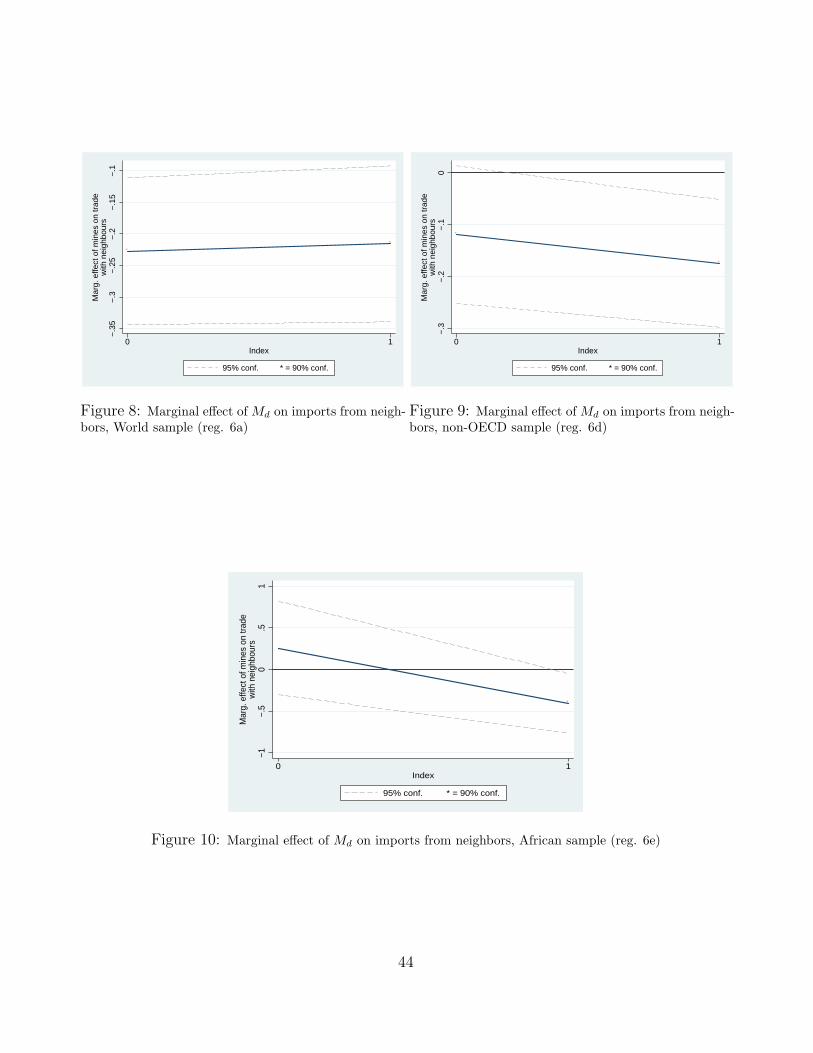
−.3

5−

.3−

.25

−.2

−.1

5−

.1

Mar

g. e

ffect

of m

ines

on

trad

ew

ith n

eigh

bour

s

0 1Index

95% conf. * = 90% conf.

Figure 8: Marginal effect of Md on imports from neigh-bors, World sample (reg. 6a)

*

*

−.3

−.2

−.1

0

Mar

g. e

ffect

of m

ines

on

trad

ew

ith n

eigh

bour

s

0 1Index

95% conf. * = 90% conf.

Figure 9: Marginal effect of Md on imports from neigh-bors, non-OECD sample (reg. 6d)

*

−1−.

50

.51

Mar

g. e

ffect

of m

ines

on

trade

with

nei

ghbo

urs

0 1Index

95% conf. * = 90% conf.

Figure 10: Marginal effect of Md on imports from neighbors, African sample (reg. 6e)

44

**

* * * * * * *** ****** * * * * ****

*

**

** * * * ***

****** * *

0.5

1M

arg.

effe

ct b

eing

nei

ghbo

rs o

n ln

trad

e

0 2 4 6ln number of mines, destination

For Index = 0 For Index = 1* = 95% conf.

Figure 11: Marginal effect of N on imports, non-OECDsample (reg. 6d)

** * * * * * * * * * * * *

*

**

* * * *

−1

01

23

Mar

g. e

ffect

bei

ng n

eigh

bors

on

ln tr

ade

0 2 4 6ln number of mines, destination

For Index = 0 For Index = 1* = 95% conf.

Figure 12: Marginal effect of N on imports, Africasample (reg. 6e)

Figure 13: Marginal effect of N on imports, non-OECDsample (reg. 7d)

Figure 14: Marginal effect of N on imports, Africasample (reg. 7e)

45

D Tables

Table 1: Imports as a share of total imports1

destination: origin: mean sd min maxOECD neighbors 29% 20% 0% 74%Africa neighbors 14% 22% 0% 89%ROW neighbors 17% 20% 0% 90%Africa Africa, non-neighbors 11% 12% 0% 57%

1 ROW is the world minus OECD and Africa. Means are means across coun-tries for 2006 bilateral trade volumes in dollars. Missing and zero bilateraltrade flows are treated as zero. I.e., 29% implies that the average OECDcountry imports a volume of its known import flows from neighboring coun-tries that represents 29% of all of its known imports.

Table 2: Imports as a share of total imports

destination: origin: mean sd min maxOECD neighbors 29% 20% 0% 74%non-OECD neighbors 16% 21% 0% 90%Africa neighbors 14% 22% 0% 89%non-Africa neighbors 19% 21% 0% 90%non-Africa, non-OECD neighbors 17% 20% 0% 90%Africa Africa, non-neighbors 11% 12% 0% 57%World neighbors 18% 21% 0% 90%

Note: Means are means across countries within the given sample for bilateral tradevolumes in dollars. Missing and zero bilateral trade flows are treated as zero. I.e., 29%implies that the average OECD country imports a volume of its known import flowsfrom neighboring countries that represents 29% of all of its known imports. The OECDmean is significantly higher than all other means. The mean of the share of imports byAfrican countries from non-neighboring African countries is significantly lower than allother means except the mean of the share of imports by African countries from neighbors.The other means are not significantly different at 95% confidence.

46

Table 3: Top mining countries and mine impact index πd

Country Mines πd Country Mines πd

United States 14090 0.29 China 93 0.56Mexico 713 0.30 Panama 85 0.82Brazil 610 0.79 South Korea 84 0.57Peru 528 0.66 India 80 0.41Argentina 416 0.60 France 75 0.38Canada 358 0.13 Philippines 57 0.05Guyana 344 0.55 Guatemala 54 0.96Colombia 337 0.34 Honduras 51 0.31Russia 314 0.27 Zimbabwe 50 0.46Australia 303 0.18 Spain 46 0.56Venezuela 254 0.35 Dominican R. 40 0.59South Africa 241 0.75 Turkey 37 0.52Uruguay 209 0.88 Laos 35 0.31Jamaica 165 0.51 Egypt 35 0.14Bolivia 161 0.08 Thailand 35 0.40Chile 159 0.06 Italy 35 0.05Japan 129 0.07 Sweden 35 0.06Cuba 129 0.09 Finland 32 0.36New Zealand 118 0.00 Germany 31 0.77Ecuador 108 0.79 Papua NG 26 0.14

Note: πd ∈ [0, 1] is an index capturing the extent to which themine-to-coast infrastructure overlaps with the location of d’s con-sumers, and thus reduces their cost of importing from overseas.

47

Table 4: Summary stats

Region Mean Md Mean πd Mean αd

Non-landlockedWorld 118.73 0.45 0.53World ex-US 38.90 0.45 0.54OECD 672.38 0.34 0.35non-OECD 31.31 0.48 0.58Africa 10.56 0.64 0.88LandlockedWorld 9.05 0.50 0.50World ex-US 9.05 0.50 0.50OECD 2.50 0.46 0.75non-OECD 10.32 0.51 0.45Africa 5.67 0.56 0.50

Note: Md equals the log of the number of mines in eachcountry, plus one; πd ∈ [0, 1] is an index capturing theextent to which the mine-to-coast infrastructure overlapswith the location of d’s consumers, and thus reduces theircost of importing from overseas; αd is a dummy equal to 1if πd is larger than its average of 0.46.

48

Table 5: The trade redirection effect of minesDep. Var. = ln trade (a) (b) (c) (d) (e)

World non-US OECD non-OECD AfricaNMd -0.222*** -0.224*** -0.135 -0.148*** -0.144

(0.051) (0.052) (0.097) (0.053) (0.184)N 1.068*** 1.059*** 0.184 0.990*** 1.258***

(0.156) (0.157) (0.337) (0.164) (0.314)ln distance -1.545*** -1.551*** -1.332*** -1.585*** -1.759***

(0.027) (0.027) (0.070) (0.030) (0.093)Shared language 0.875*** 0.888*** 0.253** 0.895*** 0.786***

(0.054) (0.054) (0.123) (0.059) (0.103)Shared legal 0.341*** 0.347*** 0.485*** 0.320*** 0.079

(0.037) (0.037) (0.074) (0.041) (0.082)ColHist 0.856*** 0.860*** 0.902*** 0.946*** 1.283***

(0.101) (0.102) (0.152) (0.123) (0.236)RTA 0.531*** 0.517*** -0.105 0.867*** 0.393***

(0.058) (0.058) (0.129) (0.072) (0.151)Both WTO 0.340*** 0.346*** 2.596*** 0.335** -0.194

(0.128) (0.128) (0.536) (0.132) (0.240)Shared currency 0.234 0.248* -0.351** 1.102*** 1.283***

(0.145) (0.146) (0.158) (0.194) (0.268)ACP -0.216*** -0.220*** -0.349*** 0.337*

(0.071) (0.071) (0.073) (0.195)

∂ ln imp/∂N = 0 forMd ≥ 3.7 3.6 0 4.4 3.6

Observations 23,122 22,933 5,063 18,059 5,571R-squared 0.730 0.727 0.805 0.697 0.679

Note: N = neighbour; NMd = Neighbour * mines in the destination country. Origin and destinationfixed effect included. Robust standard errors in parentheses: *** p< 0.01, ** p< 0.05, * p< 0.1. non-USsample excludes the US as a destination. OECD sample is OECD destinations only and non-OECDexcludes OECD countries as destinations. Africa sample refers to bilateral trade flows for which thedestination is Africa.

49

Table 6: Bias in the direction of trade and mine impact dummy

Dep. Var. = ln trade (a) (b) (c) (d) (e)World non-US OECD non-OECD Africa

NMd -0.227*** -0.231*** -0.138 -0.119* 0.259(0.059) (0.062) (0.095) (0.067) (0.287)

NMdαd 0.012 0.015 0.030 -0.055 -0.662**(0.068) (0.070) (0.136) (0.075) (0.292)

N 1.066*** 1.057*** 0.158 0.995*** 1.380***(0.156) (0.157) (0.363) (0.164) (0.305)

∂ ln imp/∂N = 0for αd = 1 & Md ≥ 3.5 3.5 0 3.6 2.1

Observations 23122 22933 5063 18059 5571R-squared 0.730 0.727 0.805 0.697 0.680

Note: N = neighbour; NMd = Neighbour * mines in the destination country; NMdαd = NMd * mineimpact index in the destination country. Origin and destination fixed effects are included, and so are thecontrols listed in Table 5. Robust standard errors in parentheses: *** p< 0.01, ** p< 0.05, * p< 0.1.non-US sample excludes the US as a destination. OECD sample is OECD destinations only and non-OECD excludes OECD countries as destinations. Africa sample refers to bilateral trade flows for whichthe destination is Africa.

50

Table 7: Larger bias in the direction of trade for non-transit countries

Dep. Var. = ln trade (a) (b) (c) (d) (e)World non-US OECD non-OECD Africa

NMd -0.218*** -0.220*** -0.135 -0.146*** -0.259(0.050) (0.052) (0.097) (0.052) (0.179)

N 0.960*** 0.951*** 0.205 0.869*** 1.310***(0.157) (0.159) (0.343) (0.164) (0.315)

NTLdMd 0.415 0.414 0.253 0.478* 1.662***(0.265) (0.266) (0.188) (0.256) (0.395)

NT 0.683* 0.685* -0.495* 0.759* -0.202(0.396) (0.397) (0.261) (0.445) (0.726)

∂ ln imp/∂N = 0for non-transit & Md ≥ 3.3& ≤ 3.6 3.3 0 3.9 2.7

Observations 23122 22933 5063 18059 5571R-squared 0.730 0.727 0.805 0.697 0.680

Note: N = neighbor; NMd = neighbor * mines in the destination country; NTLdMd = neighbor andtransit * a dummy equal to one for landlocked destination countries * mines in the destination country;NT = neighbor and transit. Origin and destination fixed effects are included, and so are the controlslisted in Table 5. Robust standard errors in parentheses: *** p< 0.01, ** p< 0.05, * p< 0.1. non-USsample excludes the US as a destination. OECD sample is OECD destinations only and non-OECDexcludes OECD countries as destinations. Africa sample refers to bilateral trade flows for which thedestination is Africa.

Table 8: Top countries with onshore oil and gas fields

Country onshore fields πOGd Country onshore fields πOG

d

Russia 143 0.11 Canada 13 0.05United States 78 0.24 Nigeria 13 0.02Iran 53 0.03 Algeria 12 0.48Saudi Arabia 41 0.11 Uzbekistan 11 0.55Iraq 26 0.63 Oman 10 0.19Libya 23 0.20 United Arab Emirates 10 0.07China 21 0.51 Kazakhstan 9 0.17Venezuela 20 0.55 Kuwait 8 0.76Mexico 15 0.01 Indonesia 8 0.30Turkmenistan 14 0.76 Colombia 7 0.42

51

Table 9: Mines and oil and gas fields

Dep. Var. = ln trade (a) (b) (c) (d) (e)World non-US OECD non-OECD Africa

NMd -0.231*** -0.233*** -0.218 -0.088 0.244(0.070) (0.072) (0.184) (0.077) (0.290)

NMdαd 0.034 0.037 0.104 -0.053 -0.616**(0.074) (0.075) (0.168) (0.080) (0.293)

NOGd 0.038 0.041 0.219 -0.059 -0.139(0.091) (0.091) (0.392) (0.092) (0.200)

NOGdαOGd -0.199 -0.200 -0.537 -0.136 -0.282

(0.146) (0.146) (0.607) (0.146) (0.385)N 1.090*** 1.078*** 0.271 1.038*** 1.455***

(0.159) (0.160) (0.418) (0.169) (0.336)

Observations 23122 22933 5063 18059 5571R-squared 0.730 0.727 0.805 0.697 0.680

Note: N = neighbour; NMd = Neighbour * mines in the destination country; NMdαd = NMd * mineimpact index in the destination country; NOGd = Neighbour * oil and gas fields in the destinationcountry; NOGdα

OGd = N)Gd * oil and gas field impact index in the destination country. Origin and

destination fixed effects are included, and so are the controls listed in Table 5. Robust standard errors inparentheses: *** p< 0.01, ** p< 0.05, * p< 0.1. non-US sample excludes the US as a destination. OECDsample is OECD destinations only and non-OECD excludes OECD countries as destinations. Africasample refers to bilateral trade flows for which the destination is Africa.1

52

E Technical Appendix - Not for Publication

E.1 Measuring the mine impact index

To measure the mine impact index we need to find first the geographical midpoint of mines in

each country (M), the urban population weighted geographical midpoint of main cities (C), the

location of the country’s main container port (P ), and the point on the shoreline nearest to point

M (S). For point M , given the latitude and longitude of each mine i in country j, we calculate

their geographic midpoint on the globe as follows:

M latj = arctan(zj,

√x2

j + y2j )/π ∗ 180

M lonj = arctan(yj, xj)/π ∗ 180,

where:

xj =∑

i

cos(latitudei ∗ π/180) ∗ cos(longitudei ∗ π/180)/Ij

yj =∑

i

cos(latitudei ∗ π/180) ∗ sin(longitudei ∗ π/180)/Ij

zj =∑

i

sin(latitudei ∗ π/180)/Ij,

and where Ij is the total number of mines with available WGS 84 coordinates in country j.

We follow a similar procedure for point C. However, instead of summing over each mine i,

we sum over each city, and weigh each city by its population in 1950.40 The data on cities comes

from the UN’s “World Urbanization Prospects” database of urban agglomerations with at least

750,000 inhabitants in 2010, to which we add hand collected city coordinates. We choose the

earliest available figure for population, because current population sizes may have been influenced

by infrastructure itself. With weights, zj becomes:∑

i sin(latitudei ∗ π/180) ∗ pi/∑

i pij where

pij is the population of city i in country j. The midpoint of cities will thereforee be relatively

closer to the largest city, reflecting the fact that infrastructure that connects cities with the main

40Results are robust to using current (2005) population.

53

port will be located mostly near larger cities.

Point P captures the location of the country’s main commercial port. To identify this point

for all countries in our sample, we proceed in several steps. First, we use the “World Port

Ranking 2009” provided by the American Association of Port Authorities (AAPA) to infer the

main container port for all countries with at least on port included in the ranking. For countries

that are not included in the AAPA ranking, we use, when possible, Maersk’s website, to track

the port used by Maersk Line - the world’s leading container shipping company - to import

a container from Shanghai into the country’s capital.41 Finally, for countries that are neither

included in the AAPA ranking nor reached by Maersk Line, we identify the main commercial

port by conducting a series of internet searches.42 We coded as “port co-ordinates” those of

the port’s nearest city, which we got from the World Urbanization Prospects database, and, for

smaller cities, from Wikipedia/GeoHack.

To find point S, the coastal point closest to the midpoint of the mines, we rely on the

“Global Self-consistent, Hierarchical, High-resolution Shoreline Database” (GSHHSD) provided

by the National Oceanic and Atmospheric Administration (NOAA).43 The database provides the

co-ordinates of all coastlines in the world, and comes in four levels of detail (1 =land, 2 =lake,

3 =island in lake, 4 =pond in island in lake) and five resolutions. For our purposes, it is best

to use level 1, which excludes the possibility that we find S on the shore of a lake, and a low

resolution, which builds up the world’s coastlines from 64, 000 coordinates.44 For each country,

we calculate the distance between point M and each coastal point, and pick S as the coastal point

that minimizes such distance. Following this procedure, point S for the mines of South Africa

is only 50km from the actual port of Durban, while point S for the mines of the Democratic

Republic of Congo turns out to be on the coast of Angola.

Having identified points M , P and S for each country in our sample, we move to calculate

the mine impact index as described in (6)-(8). To accurately measure distances between pairs

41Maersk Line has the largest market share (18%) according to http://www.shippingcontainertrader.com/facts.shtml.42This led us to take Shanghai as the reference port for Kyrgystan, Tajikistan and Mongolia, Poti for Tur-

menistan and Uzbekistan, and St Petersburg for Kazakhstan.43http://www.ngdc.noaa.gov/mgg/shorelines/gshhs.html44An intermediate level of detail would use 380, 000 coordinates, and quickly increase the time it takes to

calculate distances.

54

of points, we use navigation formulas.45 The distances MP , MS, and CP are great circle

distances.46 To find the distance MI (the distance between M and I, where I is the point on the

course from C to P that is nearest to point M) we use the great circle distance CM if point I

lies behind the stretch CP , which is when IP > CP . If point I lies on CP , we use the absolute

“cross track error”: xteCMP = | arcsin(sin(CM) ∗ sin(crsCM − crsCP ))| (with coordinates in

radians), where crsCM is the course from C to M and crsCP is the course from C to P .47 The

distance IP is then found by calculating the “along track distance”: arcsin(√{(sin(CM))2 −

(sin(xteCMP ))2}/ cos(xteCMP )).

E.2 Robustness

E.2.1 Do large countries trade more with neighbors?

The number of mines in a country depends on geology and exploration, but there is also the

possibility that larger countries have more subsoil assets per se. For example, a simple log-

linear regression of mines on surface area and income per capita yields a significant elasticity of

surface area of 0.59. In turn, because of their size and long borders, large countries may trade

disproportionately more with neighboring countries. This section explores this possibility by

adding an interaction between the log of surface area in km2 (which we label by Ad) and the

neighbor dummy to our main specification (the one reported in Table 6). The result is given

in Table 10. Larger countries do appear to trade more with neighbors than smaller countries

(except in Africa), even while controlling for the average effect of distance. However this effect

does not explain why we find a negative effect of mines on trade. In fact, since larger countries

have more mines and tend to trade more with neighbors, the trade re-direction effect is stronger

after we control for country size.

45See http://williams.best.vwh.net/avform.htm46That is, the distance between C and P is equal to arccos(sin(latc)∗ sin(latp)+cos(latc)∗cos(latp)∗cos(lonc−

lonp)), with coordinates in radians.47These can be found as: mod (arctan(sin(lonc−M lon)∗cos(M lat), cos(latc)∗sin(M lat)−sin(latc)∗cos(M lat)∗

cos(lonc −M lon)), 2π).

55

E.2.2 “Zeros in trade” and “zeros in mines”

Building on the recent literature on estimating trade flows allowing for the number of trading

partners (Helpman et al., 2008), and the econometric literature on sample selection bias as a

specification error (Heckman, 1979) we offer two-stage estimates of the determinants of both the

external and internal margin in trade. We present this as a robustness exercise because we use a

2006 cross-section of trade with relatively few “zero” observations, which means that we loose few

observations by taking the log of trade.48 Within the sample bounded by the control variables

we observe positive trade for 88 percent of possible trade flows, while for example Helpman et

al. (2008) observe only 45 percent positive values in the 1986 cross section of trade.

To tackle the problem of zeroes in trade data, we correct for sample selection bias arising

from omitted variables that measure the impact of the number of firms that engage in trade

to a particular country. We adopt an agnostic approach and specify probit equations for the

first stage to estimate the probability that a particular country exports to another country and

use the resulting predictions in the second stage to estimate the determinants of bilateral trade.

The advantage of this method is that the decision to enter foreign markets through exports and

the amount of trade are determined separately. Alternative methods such as simple OLS on the

selected sample of positive trade have to assume that both decisions are independent, while a

Tobit regression makes the strong assumption that both decisions can be captured by the same

model. The nonlinear Poisson Pseudo Maximum Likelihood model proposed by Santos Silva

and Tenreyro (2006) allows inclusion of both zero and non-zero trade flows and estimates the

combined effect of the external and the internal margin, but tends to underestimate the number

of zero flows, in addition to assuming homogenous coefficients for both entry and the amount of

trade. We favor the two-stage method but report PPML estimates as well.

Although the two-step method is not necessary to obtain consistent estimates, an instrument

is needed for otherwise the identification comes off the functional form assumption (normality).

We thus need at least one variable that determines entry in foreign markets but does not also

determine the volume of trade. We closely follow Helpman et al. (2008) who find evidence that

48The raw COMTRADE data has only positive and missing observations. An alternative source, the IMFdirections of trade database, reports mostly zeros where COMTRADE reports missing trade. We thereforeassume that missing trade represents no trade in COMTRADE as well.

56

the decision to export is well determined by measures of the cost of entry in a foreign market,

while entry costs do not affect the amount of trade.49 We offer a small improvement in that entry

cost, proxied by a dummy variable equal to one if the combined amount of days and procedures

it takes to start a business is above median, is measured in 1999 (Djankov et al., 2002) and is

therefore more likely to affect 2006 trade than 1986 trade. We start from our main specification

(the one reported in Table 6), and estimate the following two-stage model for non-resource FDI

with the Heckman (1979) correction:

Pr(impod > 0)|NodMd, NodMdαd, Nod, ln τod) = Φ(γ1NodMd + γ2NodMdαd + γ3Nod + γ ln τod)

(14)

E[ln impod|impod > 0, NodMd, NodMdαd, Nod, ln τod, ao, ad] =

= k − ln τod + ao + ad + β1NodMd + β2NodMdαd + β3Nod + ρodσodφod + vod

(15)

where Φ(.) indicates the cumulative normal density function and ρod are the correlations

between unobserved determinants of decisions to enter into trade and unobserved determinants

of trade once entry has occurred. The term φod = ϕ(.)/[1−Φ(.)] denotes the inverse Mills ratio,

where ϕ(.) denotes the standard normal density function. This ratio is included in the second

stage (15) to correct for sample selection bias and is calculated from the estimated parameters

of the first stage (14). By including the inverse Mills ratio in the second stage, estimating the

coefficients and realizing that the standard deviation σod cannot be zero, the null hypothesis that

ρodσod = 0 is equivalent to testing for sample selectivity.

Table 11 reports the result. For each region we report the first-stage probit that determines

entry into foreign markets, and the second-stage regression with the inverse Mill’s ratio. The

latter is significant in all but the OECD sample, where countries trade with most other countries.

In all cases, the first stage shows that mines make it less likely that countries trade with neighbors

49This can be rationalized using recent theories that split entry costs into fixed and variable costs, and predictthat only the most productive firms can overcome the fixed costs.

57

at all, consistently with our hypothesis; and that entry costs correlate negatively with trade.

Moving to the volume of trade in the second stage, we still find that countries with more mines

import relatively less from neighbors. Again, we find that in Africa this effect is only significant

and negative if mines have a high potential for re-directing trade (αd = 1).

For completeness, we also report the PPML estimates, which as explained above, more re-

strictively assume the same model for both margins of trade. In this case the estimates are

somewhat less significant, as shown by Table 12.

Finally, we also address censoring of the variable Md. Based on the notion that the existence

of subsoil assets - and therefore mines - depends mostly on geology (which is essentially random),

we have added one unit to the count variable of the number of mines, to prevent selection on a

sample with only non-zero mines. The second rationale for doing this is that it is unlikely that

any country truly has no mine at all, while it is probably due to random measurement error that

some mines do not appear in the MRDS data. We perform a final check and regress trade on an

interaction between neighbor and mines, where mines is the log number of mines as reported by

the US Geological Survey (Table 13). Panel A includes only NMd, while Panel B also includes

NMdαd. Selecting only countries with at least one mine leads to a sample reduction from 23120

to 16318, a reduction of 29 percent. Nevertheless, we still observe a significant trade re-direction

effect, which in Africa depends on the mine impact index as before.

58

Table 10: Large countries trade more with neighbors

Dep. Var. = ln trade (a) (b) (c) (d) (e)World non-US OECD non-OECD Africa

NMd -0.334*** -0.342*** -0.599*** -0.199*** 0.229(0.068) (0.070) (0.226) (0.077) (0.290)

NMdαd -0.000 0.005 -0.047 -0.060 -0.673**(0.069) (0.070) (0.126) (0.076) (0.294)

NAd 0.174*** 0.177*** 0.806** 0.121** 0.108(0.052) (0.052) (0.357) (0.054) (0.137)

N -0.883 -0.927 -8.475** -0.367 0.022(0.605) (0.605) (3.809) (0.622) (1.780)

Observations 23120 22931 5063 18057 5571R-squared 0.730 0.727 0.805 0.697 0.680

Note: N = neighbour; NMd = Neighbour * mines in the destination country; NMdαd = NMd * mineimpact index in the destination country.; NAd Neighbor * log area in km2 of the destination country.Origin and destination fixed effect included. Robust standard errors in parentheses: *** p< 0.01, **p< 0.05, * p< 0.1. non-US sample excludes the US as a destination. OECD sample is OECD destinationsonly and non-OECD excludes OECD countries as destinations. Africa sample refers to bilateral tradeflows for which the destination is Africa.

59

Tab

le11

:H

eckm

an2-

step

esti

mat

ion

Sam

ple:

Wor

ldno

n-U

SO

EC

Dno

n-O

EC

DA

fric

aM

etho

d:pr

obit

OL

Spr

obit

OL

Spr

obit

OL

Spr

obit

OL

Spr

obit

OL

SD

ep.

var.

istr

ade

in:∈

(0,1

)ln

∈(0,1

)ln

∈(0,1

)ln

∈(0,1

)ln

∈(0,1

)ln

1st

stag

e1s

tst

age

1st

stag

e1s

tst

age

1st

stag

eNM

d-0

.017

***

-0.2

35**

*-0

.018

***

-0.2

39**

*-0

.004

***

-0.1

32-0

.024

**-0

.141

**-0

.021

**0.

191

(0.0

06)

(0.0

62)

(0.0

06)

(0.0

62)

(0.0

01)

(0.1

10)

(0.0

10)

(0.0

66)

(0.0

10)

(0.2

95)

NM

dα

d-0

.002

0.01

3-0

.002

0.01

7-0

.003

**0.

039

0.01

4-0

.043

0.01

5-0

.629

**(0

.008

)(0

.068

)(0

.009

)(0

.068

)(0

.001

)(0

.131

)(0

.014

)(0

.076

)(0

.013

)(0

.293

)N

-0.0

23*

1.06

2***

-0.0

24*

1.05

2***

0.01

4***

0.15

4-0

.064

**0.

949*

**0.

005

1.46

0***

(0.0

14)

(0.1

72)

(0.0

14)

(0.1

72)

(0.0

04)

(0.3

90)

(0.0

25)

(0.1

73)

(0.0

11)

(0.2

89)

lndi

stan

ce-0

.053

***

-1.5

64**

*-0

.054

***

-1.5

72**

*-0

.002

***

-1.3

25**

*-0

.098

***

-1.6

58**

*-0

.033

***

-1.9

31**

*(0

.003

)(0

.031

)(0

.003

)(0

.031

)(0

.001

)(0

.071

)(0

.004

)(0

.034

)(0

.004

)(0

.096

)Sh

ared

lang

uage

0.03

1***

0.89

2***

0.03

1***

0.90

7***

0.00

20.

244*

0.05

6***

0.94

6***

0.02

7***

0.90

1***

(0.0

03)

(0.0

59)

(0.0

03)

(0.0

59)

(0.0

01)

(0.1

26)

(0.0

06)

(0.0

63)

(0.0

04)

(0.1

05)

Shar

edle

gal

0.01

0***

0.34

5***

0.01

1***

0.35

1***

0.00

1*0.

478*

**0.

018*

**0.

333*

**0.

004

0.11

6(0

.002

)(0

.040

)(0

.002

)(0

.040

)(0

.001

)(0

.075

)(0

.004

)(0

.044

)(0

.003

)(0

.083

)C

olH

ist

0.00

60.

854*

**0.

006

0.85

8***

0.00

30.

896*

**-0

.029

0.90

2***

0.23

9***

1.18

0***

(0.0

16)

(0.1

27)

(0.0

17)

(0.1

28)

(0.0

02)

(0.1

60)

(0.0

44)

(0.1

33)

(0.0

31)

(0.2

46)

RT

A0.

041*

**0.

521*

**0.

043*

**0.

506*

**0.

017*

**-0

.105

0.06

4***

0.87

7***

0.01

1*0.

313*

*(0

.007

)(0

.066

)(0

.007

)(0

.067

)(0

.003

)(0

.129

)(0

.012

)(0

.080

)(0

.006

)(0

.154

)B

oth

WT

O0.

010*

*0.

327*

*0.

010*

*0.

332*

*-0

.001

2.61

9***

0.01

30.

316*

*0.

019*

**-0

.130

(0.0

05)

(0.1

39)

(0.0

05)

(0.1

39)

(0.0

04)

(0.5

33)

(0.0

08)

(0.1

40)

(0.0

07)

(0.2

40)

Shar

edcu

rren

cy0.

008

0.23

00.

008

0.24

30.

001

-0.3

51**

0.01

11.

181*

**-0

.008

1.31

6***

(0.0

08)

(0.1

76)

(0.0

09)

(0.1

78)

(0.0

03)

(0.1

63)

(0.0

15)

(0.2

13)

(0.0

08)

(0.2

74)

AC

P-0

.025

***

-0.1

89**

*-0

.025

***

-0.1

92**

*-0

.043

***

-0.2

87**

*-0

.035

**0.

463*

*(0

.007

)(0

.072

)(0

.007

)(0

.072

)(0

.013

)(0

.074

)(0

.016

)(0

.198

)E

ntry

cost

s-0

.006

*-0

.006

*0.

001

-0.0

14**

-0.0

08*

(0.0

03)

(0.0

03)

(0.0

01)

(0.0

06)

(0.0

05)

Inve

rse

Mill

’sra

tio

0.19

4**

0.21

1**

-0.3

890.

584*

**1.

362*

**(0

.087

)(0

.088

)(0

.362

)(0

.098

)(0

.162

)

%ze

rotr

ade

22%

23%

8%26

%28

%O

bser

vati

ons

2978

323

122

2959

222

933

5476

5063

2430

718

059

7694

5571

R-s

quar

ed0.

730

0.72

70.

805

0.69

80.

685

Not

e:E

ntry

cost

sis

adu

mm

yeq

ual

toon

eif

the

sum

ofth

enu

mbe

rof

days

and

proc

edur

esth

atar

ene

cess

ary

tost

art

abu

sine

ssar

eab

ove

med

ian.N

=ne

ighb

our;NM

d=

Nei

ghbo

ur*

min

esin

the

dest

inat

ion

coun

try;NM

dα

d=NM

d*

min

eim

pact

inde

xin

the

dest

inat

ion

coun

try.

Tra

de-p

air

clus

tere

dst

anda

rder

rors

inpa

rent

hese

s:**

*p<

0.01

,**

p<0.

05,*

p<0.

1.no

n-U

Ssa

mpl

eex

clud

esth

eU

Sas

ade

stin

atio

n.O

EC

Dsa

mpl

eis

OE

CD

dest

inat

ions

only

and

non-

OE

CD

excl

udes

OE

CD

coun

trie

sas

dest

inat

ions

.A

fric

asa

mpl

ere

fers

tobi

late

ral

trad

eflo

ws

for

whi

chth

ede

stin

atio

nis

Afr

ica.

60

Table 12: Poisson PMLE estimatesDep. var.= trade, with .=0 (a) (b) (c) (d) (e)

Panel A World non-US OECD non-OECD AfricaNMd -0.000 -0.061* 0.012 -0.152*** -0.213**

(0.026) (0.034) (0.026) (0.036) (0.096)N 0.291*** 0.412*** 0.397*** 0.680*** 1.162***

(0.112) (0.124) (0.121) (0.158) (0.324)

Panel B World non-US OECD non-OECD AfricaNMd 0.000 -0.064* 0.013 -0.166*** -0.192*

(0.026) (0.038) (0.026) (0.039) (0.113)NMdαd -0.011 0.014 -0.006 0.030 -0.027

(0.033) (0.035) (0.034) (0.036) (0.111)N 0.301*** 0.405*** 0.404*** 0.679*** 1.162***

(0.116) (0.124) (0.125) (0.157) (0.324)

% zero trade 22% 23% 8% 26% 28%Observations 29783 29592 5476 24307 7694

Note: N = neighbour; NMd = Neighbour * mines in the destination country; NMdαd = NMd *mine impact index in the destination country. Origin and destination fixed effect included. Robuststandard errors in parentheses: *** p< 0.01, ** p< 0.05, * p< 0.1. non-US sample excludes the US asa destination. OECD sample is OECD destinations only and non-OECD excludes OECD countries asdestinations. Africa sample refers to bilateral trade flows for which the destination is Africa.

61

Table 13: Observations with only non-zero mines

Dep. Var. = ln trade (a) (b) (c) (d) (e)Panel A World non-US OECD non-OECD AfricaNMd -0.268*** -0.272*** -0.181* -0.206*** 0.004

(0.056) (0.058) (0.094) (0.062) (0.240)N 1.315*** 1.310*** 0.222 1.237*** 1.079**

(0.194) (0.196) (0.309) (0.222) (0.465)

Observations 16,318 16,129 4,347 11,971 3,857R-squared 0.736 0.732 0.805 0.702 0.699

Panel B World non-US OECD non-OECD AfricaN -0.275*** -0.282*** -0.180* -0.180** 0.341

(0.064) (0.067) (0.093) (0.075) (0.327)NMdαd 0.016 0.020 -0.012 -0.050 -0.629**

(0.069) (0.070) (0.136) (0.076) (0.310)N 1.311*** 1.306*** 0.233 1.243*** 1.261***

(0.194) (0.196) (0.321) (0.223) (0.451)

Observations 16318 16129 4347 11971 3857R-squared 0.736 0.732 0.805 0.702 0.700

Note: N = neighbour; NMd = Neighbour * mines in the destination country. Origin and destinationfixed effect included. Robust standard errors in parentheses: *** p< 0.01, ** p< 0.05, * p< 0.1. non-USsample excludes the US as a destination. OECD sample is OECD destinations only and non-OECDexcludes OECD countries as destinations. Africa sample refers to bilateral trade flows for which thedestination is Africa.

62