From Laser Scanner point clouds to 3D modeling of the ...
67
Hochschule Karlsruhe – Technik und Wirtschaft University of Applied Sciences Fakultät für Fakultät für Informationsmanagement und Medien Master´s Programme Geomatics Master´s Thesis of María Cristina Gómez Peribáñez FROM LASER SCANNER POINT CLOUDS TO 3D MODELING OF THE VALENCIAN SILO-YARD IN BURJASSOT First Referee: Prof. Dr.-Ing. H. Saler Second Referee: Prof. Dr.-Ing. V. Tsioukas (AUTH) Third Referee: Prof. Dr.-Ing. F. Buchón (UPV) Karlsruhe, September 2017
Transcript of From Laser Scanner point clouds to 3D modeling of the ...

Hochschule Karlsruhe – Technik und Wirtschaft
University of Applied Sciences
Fakultät für Fakultät für Informationsmanagement und Medien
Master´s Programme Geomatics
Master´s Thesis
of
María Cristina Gómez Peribáñez
FROM LASER SCANNER POINT CLOUDS TO 3D MODELING
OF THE VALENCIAN SILO-YARD IN BURJASSOT
First Referee: Prof. Dr.-Ing. H. Saler
Second Referee: Prof. Dr.-Ing. V. Tsioukas (AUTH)
Third Referee: Prof. Dr.-Ing. F. Buchón (UPV)
Karlsruhe, September 2017

I | P a g e
Acknowledgement
I would like to express my sincere thanks to all those who have
made this Master Thesis possible, especially to the program Baden-
Württemberg Stipendium.
I would like to thank my tutors Heinz Saler, Vassilis Tsioukas and
Fernando Buchón, for the time they have given me, for their help and
support in this project.
To my parents, family and friends, I would also like to thank you for
your daily support to complete this project. Especially to Irini for all her
help.
Thanks.
María Cristina Gómez Peribáñez

Hochschule Karlsruhe – Technik und Wirtschaft
Aristotle University of Thessaloniki -Faculty of Engineering
University Polytechnic of Valencia
1 | P a g e
Table of contents
Acknowledgement ......................................................................................................................... I
Table of contents .......................................................................................................................... 1
List of figures ................................................................................................................................ 3
List of tables ................................................................................................................................. 6
Introduction ................................................................................................................................... 7
1. Introduction ........................................................................................................................ 7
2. Justification ........................................................................................................................ 7
Main part ...................................................................................................................................... 8
3. Theoretical basis ............................................................................................................... 8
3.1. 3D Laser scanning ..................................................................................................... 8
3.2. Point cloud processing ............................................................................................... 8
3.3. 3D modeling ............................................................................................................... 9
4. Location of research ........................................................................................................ 10
4.1. Meaning of “Silo” ...................................................................................................... 11
4.2. Cultural and historical significance of Valencian Silo-Yard ...................................... 11
5. Material resources and technical equipment ................................................................... 13
6. Description of the primary data collection process .......................................................... 14
6.1. Primary data collection ............................................................................................. 14
7. Methodology .................................................................................................................... 15
7.1. Model of data analysis .............................................................................................. 15
7.2. Schedule of activities ................................................................................................ 16
7.3. Processing with SCENE to align the raw point clouds ............................................. 17
7.3.1. Description of the SCENE software .................................................................. 17
7.3.2. Align Scans ....................................................................................................... 18
7.3.3. Colorize scans ................................................................................................... 22
7.3.4. Deleted points which not belong to the model .................................................. 23
7.3.5. Create the Point Cloud from Scans ................................................................... 25
7.3.6. Export final data ................................................................................................ 25
7.4. Processing with CloudCompare to georeferencing the point clouds ........................ 26
7.4.1. Description of the CloudCompare software ...................................................... 26
7.4.2. Register between two clouds ............................................................................ 26
7.4.3. Estimation error after transformation ................................................................. 28
7.4.4. TLS Scans Georeferenced ................................................................................ 29
7.4.5. Export final data ................................................................................................ 29
7.5. Processing with 3DReshaper to generate the 3D model ......................................... 30
7.5.1. Description of the 3DReshaper software .......................................................... 30

Hochschule Karlsruhe – Technik und Wirtschaft
Aristotle University of Thessaloniki -Faculty of Engineering
University Polytechnic of Valencia
2 | P a g e
7.5.2. Merge data by zones ......................................................................................... 33
7.5.3. Subdivide the point clouds in Silos and corridors (P0) ...................................... 35
7.5.4. Delete the electrical installation and targets (P1) .............................................. 38
7.5.5. Automatically filter data noise (P2) .................................................................... 41
7.5.6. Create 3D mesh (P3) ........................................................................................ 42
7.5.7. Smooth the mesh (P4) ...................................................................................... 43
7.5.8. Colorize or texturing the mesh (P5) .................................................................. 43
7.5.9. Merging all the meshes ..................................................................................... 46
7.5.10. Reduced mesh .............................................................................................. 47
7.5.11. Translated mesh ............................................................................................ 48
7.5.12. Scripts with 3DReshaper ............................................................................... 49
7.5.13. Some problems or errors detected ................................................................ 49
7.6. Processing with Agisoft PhotoScan to create the texture ......................................... 51
7.6.1. Description of the Agisoft PhotoScan ................................................................ 51
7.6.2. Generated the orthomosaic in RGB .................................................................. 51
7.6.3. Applied the thermal images to the 3D model .................................................... 54
7.7. Processing with Blender to create the virtual reality ................................................. 56
7.7.1. Description of the Blender software .................................................................. 56
7.7.2. Compacting the images of a 3D model ............................................................. 56
7.7.3. Create virtual reality .......................................................................................... 58
7.7.4. Export final data ................................................................................................ 60
7.7.5. The game’s instructions .................................................................................... 61
Conclusion .................................................................................................................................. 62
8. Conclusion ....................................................................................................................... 62
References ................................................................................................................................. 63
9. References ...................................................................................................................... 63
Appendix I: Silo Volume in Plan View ........................................................................................ 65

Hochschule Karlsruhe – Technik und Wirtschaft
Aristotle University of Thessaloniki -Faculty of Engineering
University Polytechnic of Valencia
3 | P a g e
List of figures
Figure 4.1. Location map of the Burjassot municipality (Valencia-loc.svg 2010) ....................... 10
Figure 4.2. Bird’s-eye-view of the Valencian Silo-Yard (Bing maps 2017) ................................ 10
Figure 4.3. Public transport near the Valencian Silo-Yard (Google Maps 2017). ...................... 10
Figure 4.4. Cross section of the Valencian Silo-Yard, where underground granaries and buildings are depicted (Valls, 2014). .......................................................................................... 11
Figure 6.1. Inside Scans (22 scans, left) and outside Scans (51 scans, right) of the Valencia Silo-Yard ..................................................................................................................................... 14
Figure 7.1. Processing scheme to obtain the 3D model ............................................................. 15
Figure 7.2. Gantt diagram of the 3D Modeling in Valencian Silo-Yard (Smartsheet 2016). ....... 16
Figure 7.3. Sensors properties “Silos022” (left) and “Silos028” (right) with measure of GPS (SCENE) ..................................................................................................................................... 18
Figure 7.4. Correspondence view of “Silos 022” (green) and “Silos028” (red) (SCENE) ........... 18
Figure 7.5. Incorporate new points and force correspondences between shown scans” by hand (SCENE) ..................................................................................................................................... 19
Figure 7.6. Place scan by Target Based (SCENE) .................................................................... 19
Figure 7.7. Transformation and correspondence view, before place scan “Silos012” (SCENE) 20
Figure 7.8. Target common between two scans (“Silos022” – “Silos021”) (SCENE) ................. 20
Figure 7.9. Correspondence view all scans inside (SCENE) ..................................................... 21
Figure 7.10. Correspondence view, place scans between 023 and 039, added the new scans between 041 and 060 (SCENE) ................................................................................................. 21
Figure 7.11. Error in the “Place Scans” with “Silos058”, “Silos054” and “Silos060” (SCENE) ... 21
Figure 7.12. Correspondence view after finished the place scan (SCENE) ............................... 22
Figure 7.13. Results of the final place scan by top view (SCENE) ............................................. 22
Figure 7.14. Before and after of delete the scattered points outside (SCENE) .......................... 23
Figure 7.15. Planar View outside (left) and inside (right) the Valencian Silo-Yard (SCENE) ..... 23
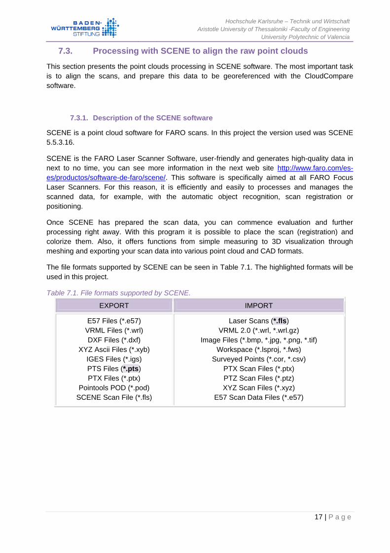
Figure 7.16. Selection zone in planar view outside (left) and inside (right) the Valencian Silo-Yard (SCENE) ............................................................................................................................ 24
Figure 7.17. 3D View of the selected zone of the scan outside (left) and inside (right) the Valencian Silo-Yard (SCENE) .................................................................................................... 24
Figure 7.18. Selection polygon with the invalid data points outside (left) and inside (right) the Valencian Silo-Yard (SCENE) .................................................................................................... 24
Figure 7.19. Selection polygon with the incorrect points from the scanner (SCENE) ................ 24
Figure 7.20. Create Point Cloud and 3D view (SCENE) ............................................................ 25
Figure 7.21. Export scans in PTS file (SCENE) ......................................................................... 25
Figure 7.22. Open point clouds in PTS format (CloudCompare) ................................................ 26
Figure 7.23. Registration values of UAV cloud (reference) and TLS cloud (CloudCompare) .... 27
Figure 7.24. Transformation matrix TLS to UAV (CloudCompare) ............................................. 27
Figure 7.25. Transformation matrix TLS to UAV in TXT file (Notepad++) .................................. 27
Figure 7.26. View of the TLS point cloud colorize by distance and histogram by approximate distances (CloudCompare) ......................................................................................................... 29

Hochschule Karlsruhe – Technik und Wirtschaft
Aristotle University of Thessaloniki -Faculty of Engineering
University Polytechnic of Valencia
4 | P a g e
Figure 7.27. Parameters to export the PTS format compatible with 3DReshaper (CloudCompare) ................................................................................................................................................... 29
Figure 7.28. Range of features include in the software 3DReshaper (3D Reshaper 2015). ...... 30
Figure 7.29. Schema about which scan belongs to each zone .................................................. 33
Figure 7.30. Diagram of the processes in 3DReshaper ............................................................. 34
Figure 7.31. Filter clouds, noise reduction (3DReshaper 17.0.6.24515) .................................... 35
Figure 7.32. Schema of the location and numbering of each silo and corridor (orthophoto (Soubry 2016)) ........................................................................................................................... 35
Figure 7.33. Selected cloud to separate Corridor_01 (left) and Silo_01 (right) (3DReshaper) .. 36
Figure 7.34. Example of noise elimination in 3DReshaper (3DReshaper) ................................. 36
Figure 7.35. Selected clouds to merge in a cloud “Corridor_01” (3DReshaper) ........................ 36
Figure 7.36. Scans inside of the building (3DReshaper) ............................................................ 37
Figure 7.37. Planes perpendicular to every silo (3DReshaper) .................................................. 37
Figure 7.38. Separating the corridor into two parts (3DReshaper) ............................................. 38
Figure 7.39. Example of the electrical installation and targets to be deleted (3DReshaper) ...... 38
Figure 7.40. Data segmentation with default value (3DReshaper) ............................................. 39
Figure 7.41. Fragment segmentation 5mm (3DReshaper) ......................................................... 39
Figure 7.42. First point cloud of wall (left) and first point cloud of electrical installation (right) (3DReshaper) ............................................................................................................................. 39
Figure 7.43. Non-optimal segmentation (3DReshaper) .............................................................. 40
Figure 7.44. Manually separating of electrical installation (3DReshaper) .................................. 40
Figure 7.45. Process of removing parts of the targets (3DReshaper) ........................................ 40
Figure 7.46. Delete noise from the stairs (3DReshaper) ............................................................ 41
Figure 7.47. RGB picture of the plastic cover (Valenciabonita 2017), before to deleting the noise (left), and deleting the noise of the plastic cover (right) (3DReshaper) ...................................... 41
Figure 7.48. Noise reduction iteration 1, points to delete (blue) (3DReshaper) ......................... 42
Figure 7.49. Filled holes before (left) and after (right) (3DReshaper) ........................................ 42
Figure 7.50. Refined mesh to 3mm before (left) and after (right) (3DReshaper) ....................... 43
Figure 7.51. Mosaics of Silo_01 ................................................................................................. 45
Figure 7.52. Insert reference points to texturing the mesh (3DReshaper) ................................. 45
Figure 7.53. Adjusting the textures in the silo (3DReshaper) ..................................................... 46
Figure 7.54. Joined two mesh (3DReshaper) ............................................................................. 46
Figure 7.55. Comparing between the original mesh and the reduced mesh 1mm (3DReshaper) ................................................................................................................................................... 48
Figure 7.56. Separate the first three silos of the reduced mesh of 1 mm (3DReshaper) ........... 48
Figure 7.57. Translated mesh (3DReshaper) ............................................................................. 48
Figure 7.58. Scanner error (3DReshaper) .................................................................................. 50
Figure 7.59. Removed the Scanner error (3DReshaper) ........................................................... 50
Figure 7.60. OBJ file imported into Geomagic (left) and imported into Blender (right) (Geomagic Studio 2014, Blender v2.78) ....................................................................................................... 50
Figure 7.61. Dazzled image (left) and corrected image (right) (Photoshop) .............................. 54

Hochschule Karlsruhe – Technik und Wirtschaft
Aristotle University of Thessaloniki -Faculty of Engineering
University Polytechnic of Valencia
5 | P a g e
Figure 7.62. Aligned photos of the thermal images of “Silo_01” (Agisoft PhotoScan) ............... 54
Figure 7.63. Creating the final thermal texture of the 3DReshaper model (Agisoft PhotoScan) 55
Figure 7.64. Comparison of the original mesh with the PhotoScan texture mesh (3DReshaper) ................................................................................................................................................... 55
Figure 7.65. “Smart UV project” executed (Blender 2.78) .......................................................... 57
Figure 7.66. Recommended resolution values (left) and creation of the new image (right) (Blender) ..................................................................................................................................... 57
Figure 7.67. Baked texture of the “Silo_01” (Blender) ................................................................ 57
Figure 7.68. Assigning the new texture of an image (Blender) .................................................. 58
Figure 7.69. Cube parent with the camera and the light as children (Blender) .......................... 58
Figure 7.70. Game logic of the cube (camera) (Blender) ........................................................... 59
Figure 7.71. Silos color game logic by pressing the number “1” (Blender) ................................ 59
Figure 7.72. Efficiency of the virtual reality of the silos (Blender) ............................................... 60
Figure 7.73. Explicative diagram of the emplacement of the silos in the Valencian Silo-Yard ... 60
Figure Appendix I. Silo Volume in Plan View (3DReshaper) ..................................................... 65

Hochschule Karlsruhe – Technik und Wirtschaft
Aristotle University of Thessaloniki -Faculty of Engineering
University Polytechnic of Valencia
6 | P a g e
List of tables
Table 5.1. Features of Focus 3D X 130 (FARO n.d.). ................................................................ 13
Table 7.1. File formats supported by SCENE. ........................................................................... 17
Table 7.2. View of the point cloud aligned in three points distributed on the square (CloudCompare) ......................................................................................................................... 28
Table 7.3. File formats of Point Cloud supported by 3DReshaper (3D Reshaper 2015). .......... 31
Table 7.4. File formats of Mesh supported by 3DReshaper (3D Reshaper 2015). .................... 32
Table 7.5. Sample of a 3D silo model but with different textures (3DReshaper) ........................ 43
Table 7.6. Samples of different grade of reduction (3DReshaper) ............................................. 47
Table 7.7. Script to save the point clouds (3DReshaper) ........................................................... 49
Table 7.8. Process of generating the interior texture in RGB (Agisoft PhotoScan) .................... 51

Hochschule Karlsruhe – Technik und Wirtschaft
Aristotle University of Thessaloniki -Faculty of Engineering
University Polytechnic of Valencia
7 | P a g e
Introduction
1. Introduction
This Master-Thesis Project is named “From Laser Scanner point clouds to 3D modeling of the
Valencian Silo-Yard in Burjassot”. The principal objective is promoting the cultural heritage
through geomatics. In this way, the 3D model will be established in the Valencian Silo-Yard.
The topic of this thesis is to give significance to the responsibility of cultural heritage through
geomatics. This is within the “Tri-national Cultural Heritage Documentation projects (2015-
2018)”. Taken part in the framework of the Baden-Württemberg-STIPENDIUM for university
students – BWS plus, a program of the Baden-Württemberg Stiftung. In addition, this thesis
supports the importance of proceeding to updating the data processing.
The purpose or finality of this Master Thesis is to create a virtual reality of the 3D model of the
Valencian Silo-Yard, using the data obtained in April of 2016 from the Laser Scanner and the
pictures to take the color for the 3D model.
2. Justification
This project is carried out to transfer the great importance of the implementation of Geomatics
non-destructive techniques, in order to define the characteristics and help to analyze the
Valencian Silo-Yard. Including the use of non-destructive techniques, the historical
constructions are preserved. In addition, this project is carried out to transfer what has been
learned, explaining how a real project can be developed under normal conditions.
The contribution of this document is to transfer exactly how it might be constructing a 3D model.
Additionally, with this task, my double degree studies will be completed in the “International
Master Program of Geomatics” of the University of Applied Sciences (Hochschule Karlsruhe),
and in turn, in the “Master in Geomatic and Geographic information engineering” of the
University Polytechnic of Valencia.
It is hoped that with this type of projects more people in the community can benefit and this also
could help to generate new 3D models by other professionals.
In this kind of projects it is possible that there are limitations with the software, because it will
need to process many point clouds of all the Scans of the work. For example, this project had
around 70 scans. However, the common possibility is that the hardware has not enough
memory.

Hochschule Karlsruhe – Technik und Wirtschaft
Aristotle University of Thessaloniki -Faculty of Engineering
University Polytechnic of Valencia
8 | P a g e
Main part
3. Theoretical basis
This section explains the theoretical background of this project in different areas of interest.
3.1. 3D Laser scanning
3D laser scanners are being considered in many application areas ranging from cultural
heritage documentation, industry and manufacturing, surveying to medicine. Terrestrial Laser
Scanning (TLS) is a non-invasive measurements that works on basic principles of measuring
the distance from the sensor to the surface of an object. This is the same principle as LIDAR
(Light Detection and Ranging) system.
From a 3D point cloud measured with TLS, it allows to make a complex and accurate 3D model
of an object in relatively short time. If the TLS isn’t equipped with high-resolution digital camera,
it must take precisely photographs, to obtain a model of an object with true color representation.
Some advantages from the 3D Laser Scanning are that a dense point cloud is faster obtained
with precision and accuracy. And some disadvantages of large areas are inefficiency when
captured and time-consuming work (Setkowicz, 2014).
3.2. Point cloud processing
A point cloud is a representation in three dimensions of an object or environment. Registration
is the process where two or more point clouds are aligned into one single cloud, it is required
that some common features are shared by multiple scans.
In order to avoid incomplete point clouds, several scans are required and registered to obtain an
acceptable point cloud.
It depends on the registration software if it requires or not specific reference targets. If the
software has a target-free registration process, it relies on surfaces and corners captured in
multiple scans. Two common specific reference target types are spheres and checkerboards
placed in the scanned environment.
The spheres have a highly reflective surface, a known diameter and precise roundness. The
spherical shape allows the target to be scanned from any direction and accurate localization of
the sphere centre point which is then used as reference point.
The checkerboard target consists of two black squares in checkerboard formation printed. This
target is not properly acquired when placed in a steep angle in reference to the scanner, for this
reason, the targets placement require careful planning in order to achieve good results. The
centre intersection point is used as a reference point by the registration software.
In the scanned area invalid artifacts and invalid data points are usually found. These
disturbances generated error in the point clouds measured by a 3D laser scanner. Also, spatial
data from adjacent areas is considered to be present in the scanned area as defective points.

Hochschule Karlsruhe – Technik und Wirtschaft
Aristotle University of Thessaloniki -Faculty of Engineering
University Polytechnic of Valencia
9 | P a g e
With the use of filters erroneous points are eliminated and it is complemented by manual
deletion of incorrect points.
Point clouds usually are vast which in turn requires large amounts of RAM, a powerful CPU and
adequate GPU for a smooth handling process. Depending on the data set, this process can be
extremely taxing for computer hardware (Rex & Stoli, 2014).
3.3. 3D modeling
This section focuses mostly on the generation of the polygonal surface, triangulation or mesh
generation. It is the core part of almost all reconstruction programs.
The triangulation based on a conversion of a set of points into a polygonal model (mesh). This
operation usually generates vertices, edges and faces. These components together make up
the small elements, in two dimensions they are triangles or quadrilaterals and in the three
dimensions they are tetrahedrons. Therefore, the triangulation can be performed in 2D or in 3D,
according to the geometry of the input data. However, this project is only focus in the 3D.
The results of 3D triangulation are much more complicated than a 2D triangulation. The input
data could be simple polyhedron (sphere), non-simple polyhedron (torus) or point clouds. In this
case point clouds are used.
Usually the polygons created need some post-processing operations mainly manually, for
example, refinements to correct imperfections or errors in the surface and single triangles
editing.
Certain operations consist in edges correction, triangle insertion or polygons editing. The edges
correction process allows that the faces can be split, contracted or moved to another location.
The triangles insertion method allows that the holes can be filled constructing polygonal
structures that respect the area around. Also, this method through radial basis function or
volumetric approach can be repaired incomplete meshes. The polygons editing operation
allows that the number of polygons can be reduced, preserving the shape of the object or fixing
boundary points. Also, the polygonal model can be improved adding new vertices and adjusting
the coordinates of existing vertices. Moreover spikes can be removed with smooth functions.
Generally these editing operations to refine and perfect the polygonal surface when the model
was created where applied (Remondino, 2003).

Hochschule Karlsruhe – Technik und Wirtschaft
Aristotle University of Thessaloniki -Faculty of Engineering
University Polytechnic of Valencia
10 | P a g e
4. Location of research
The study site is in the Valencian Silo-Yard, which is located in the Burjassot municipality, in
Valencia province, Spain. This can be seen in Figure 4.1.
Figure 4.1. Location map of the Burjassot municipality (Valencia-loc.svg 2010)
The bird eye view of the Valencian Silo-Yard can be seen in Figure 4.2.
Figure 4.2. Bird’s-eye-view of the Valencian Silo-Yard (Bing maps 2017)
It is located in the centre of the town and it is very accessible by public transport from Valencia,
for example, tram or metro (Figure 4.3). The tram stations of line 4 near the Valencian Silo-
Yard are “La Granja”, “Sant Joan” or “Campus”. And the closest metro station is “Burjassot (line
1).
Figure 4.3. Public transport near the Valencian Silo-Yard (Google Maps 2017).

Hochschule Karlsruhe – Technik und Wirtschaft
Aristotle University of Thessaloniki -Faculty of Engineering
University Polytechnic of Valencia
11 | P a g e
The position of the Valencian Silo-Yard in EPSG 25830, that is, ETRS89 UTM Zone 30N, the
North coordinate is “722514”, and the East coordinate is “4376472”. Furthermore, geographic
coordinates in geodetic system WGS-84, on the one hand, as decimal degrees the latitude is
“39º.5090” and the longitude is “-0º.4118”. On the other hand, expressed in degrees, minutes
and seconds, the latitude is 39°30'32"N and the longitude is 00°24'42"W.
4.1. Meaning of “Silo”
“Silo” according to “Real Academia Española” has the following three meanings. The first
meaning says dry place where wheat or other grains, seeds or fodder are stored. The second
meaning says underground, deep and dark. And the thirdly meaning says it is an underground
missile tank.
In this project the meaning of “Silo” is combination of the first and second meaning. Therefore,
in this case “Silo” means that it is a dry, underground, deep and dark place where wheat are
stored.
4.2. Cultural and historical significance of Valencian Silo-Yard
The “Silos” are subterranean granaries excavated on the top of a hill for cereal preservation, in
this case wheat in order to prevent rainwater accumulation and hydrothermal conditions for
wheat preservation.
The following description presents the standard silo morphology in the Valencian Silo-Yard. The
shape is similar to a bottle with a wide chamber and a narrow cylindrical neck at the top. The
entrance of the underground space consists of a small circular mouth of 60-70 cm diameter,
after that, the neck is a small narrow downward of 0.80 – 1.00 m deep. The diameter is 4 – 8 m
and 5.5 – 12 m deep, including the neck, in a clay soil. In these underground barns there was
capacity from 30 m3 to 260 m3. The Figure 4.4 can help us understand the meaning of “Silo” of
Valencian Silo-Yard.
Figure 4.4. Cross section of the Valencian Silo-Yard, where underground granaries and
buildings are depicted (Valls, 2014).

Hochschule Karlsruhe – Technik und Wirtschaft
Aristotle University of Thessaloniki -Faculty of Engineering
University Polytechnic of Valencia
12 | P a g e
The underground grain storage for wheat preservation was very important for the population
subsistence. In 1573, following this purpose, it was constructed in Burjassot a region that was
selected owing to favorable economic, geographical, topographic and geological aspects; it is 5
km away from Valencia downtown. The wheat stored in the Middle Ages was brought in from
Castile (Central-Spain) using terrestrial transport, as well as from Sicily through shipment.
Throughout history, the total number of former excavated silos in the Valencian Silo-Yard could
have reached 49 silos, but some of these ruined silos were buried.
The Valencian silos fell in disuse because of the 1936-39 Spanish Civil War and the introduction
of new industrial techniques. Since then, the architectural underground ensemble completely
lost its original use and it led to evolutionary deterioration (Valls, 2014).

Hochschule Karlsruhe – Technik und Wirtschaft
Aristotle University of Thessaloniki -Faculty of Engineering
University Polytechnic of Valencia
13 | P a g e
5. Material resources and technical equipment
This section presents the resources used in the development of the project, differentiating the
resources used in field work that the resources used in cabinet work.
During the period of field work it was necessary to take the data:
- Laser Scanner: FARO Focus 3D X130 (Table 5.1) Table 5.1. Features of Focus 3D X 130 (FARO n.d.).
Range Focus3D X 130 0.6 – 130 m
Measurement speed Up to 976,000 points / second
Ranging error ± 2 mm
Integr. colour camera Up to 70 mio. pixel
Laser class Laser class 1
Weight 5,2 kg
Multi-Sensor GPS, Compass, Height Sensor, Dual Axis Compensator
Size 240 x 200 x 100 mm
Scanner control Via touch-screen display and WLAN
- Tripod - Targets check-board - Polyester spheres - Second battery
During the period of cabinet in this type of project, it is usually required to have a software to
process the raw data from the Laser Scanner, in this project SCENE was used. But also, there
exist other software for processing the scans, for example, Cyclone (Leica Cyclone 3D Point
Cloud Processing Software), or CloudCompare that is a free software.
The software required in terms of modeling the data is 3DReshaper, Geomagic or Polyworks.
And the free software for 3D animation is Blender or Unit.
Therefore, in this master thesis the necessary software that will be used in this project is
SCENE, CloudCompare, Agisoft PhotoScan, 3DReshaper, Blender and Notepad ++, among
other.

Hochschule Karlsruhe – Technik und Wirtschaft
Aristotle University of Thessaloniki -Faculty of Engineering
University Polytechnic of Valencia
14 | P a g e
6. Description of the primary data collection process
This section presents some process to collect the primary data. The following is a short
description of the main points to think before starting out in the field. These are:
- Strategy planning about the places where it is necessary to put the Laser Scanner to take measurements, using orthophotos from official agency. In this case “Valencian Cartographic Institute” (http://www.icv.gva.es/va/inicio ).
- Also, it is necessary to visit the object of study place. To know their characteristics and the real situation. For instance, inside of the Silos, because it is impossible to see in the orthophotos.
- It should be noted that the scans will have a minimum overlapping with each other. To be obtained an aligned effective.
After that, the work could be executed in the field. In general, the first task is to review if the
planned positions of the Laser Scanner in the previous study are fine. And put the targets in the
place of the measurement.
Finally, outside of the building about 50 scans are registered with GPS position integrated in the
FARO Laser Scanner. And inside of the building about 23 scans are registered without GPS
position.
This project took part in the “Tri-national Cultural Heritage Documentation projects (2015-2018)”,
the work in the field was made by the students that participated in the program the last year.
These data were used to do the 3D model this year. In addition, this year we will did the
measurements in the archaeological excavation area in Vergina (Greece), this is the next step
in the "Tri-national Cultural Heritage Documentation projects (2015-2018).
In this case, the data collection took place in Burjassot, from 14th to 15th April 2016.
6.1. Primary data collection
The primary data used in this project are the registered 22 inside scans (Figure 6.1, left), 51
outside scans (Figure 6.1, right) at the Valencian Silo-Yard (Burjassot), and the images inside
the silos.
Figure 6.1. Inside Scans (22 scans, left) and outside Scans (51 scans, right) of the Valencia
Silo-Yard

Hochschule Karlsruhe – Technik und Wirtschaft
Aristotle University of Thessaloniki -Faculty of Engineering
University Polytechnic of Valencia
15 | P a g e
7. Methodology
This section explains the methodology of how to perform the processes to create the 3D model
using the Laser Scanner data. The methodological framework is defined in the following
sections through the process with different software. For example, SCENE software is for
processing Laser Scan data, … .
7.1. Model of data analysis
This section presents the model analysis using the primary data (Figure 7.1).
Figure 7.1. Processing scheme to obtain the 3D model
•Import
•Align, delete noise
•Export Point Cloud
SCENE
(Point Cloud)
•Georreferencing Point Cloud
•Estimation error
CloudCompare
(Point Cloud) •Import Images
•Create orthomosaics
•Edit images with Photoshop
•Export
Photoscan
(Images)
•Import , filter noise
•Process 3D mesh
•Textured 3D model
•Export 3D model
3DReshaper
(3D Model)
•Import
•Create the virtual realiy of the 3D model
•Export virtual reality
Blender
(3D Animation)

Hochschule Karlsruhe – Technik und Wirtschaft
Aristotle University of Thessaloniki -Faculty of Engineering
University Polytechnic of Valencia
16 | P a g e
7.2. Schedule of activities
This section presents the schedule of activities thought Gantt diagram. In this diagram (Figure
7.2), specifying the activities in function of the time, sequentially, from the starting date until the
finish date.
Figure 7.2. Gantt diagram of the 3D Modeling in Valencian Silo-Yard (Smartsheet 2016).
Hochschule Karlsruhe – Technik und Wirtschaft
Aristotle University of Thessaloniki -Faculty of Engineering
University Polytechnic of Valencia
17 | P a g e
7.3. Processing with SCENE to align the raw point clouds
This section presents the point clouds processing in SCENE software. The most important task
is to align the scans, and prepare this data to be georeferenced with the CloudCompare
software.
7.3.1. Description of the SCENE software
SCENE is a point cloud software for FARO scans. In this project the version used was SCENE
5.5.3.16.
SCENE is the FARO Laser Scanner Software, user-friendly and generates high-quality data in
next to no time, you can see more information in the next web site http://www.faro.com/es-
es/productos/software-de-faro/scene/. This software is specifically aimed at all FARO Focus
Laser Scanners. For this reason, it is efficiently and easily to processes and manages the
scanned data, for example, with the automatic object recognition, scan registration or
positioning.
Once SCENE has prepared the scan data, you can commence evaluation and further
processing right away. With this program it is possible to place the scan (registration) and
colorize them. Also, it offers functions from simple measuring to 3D visualization through
meshing and exporting your scan data into various point cloud and CAD formats.
The file formats supported by SCENE can be seen in Table 7.1. The highlighted formats will be
used in this project.
Table 7.1. File formats supported by SCENE.
EXPORT IMPORT
E57 Files (*.e57)
VRML Files (*.wrl)
DXF Files (*.dxf)
XYZ Ascii Files (*.xyb)
IGES Files (*.igs)
PTS Files (*.pts)
PTX Files (*.ptx)
Pointools POD (*.pod)
SCENE Scan File (*.fls)
Laser Scans (*.fls)
VRML 2.0 (*.wrl, *.wrl.gz)
Image Files (*.bmp, *.jpg, *.png, *.tif)
Workspace (*.lsproj, *.fws)
Surveyed Points (*.cor, *.csv)
PTX Scan Files (*.ptx)
PTZ Scan Files (*.ptz)
XYZ Scan Files (*.xyz)
E57 Scan Data Files (*.e57)

Hochschule Karlsruhe – Technik und Wirtschaft
Aristotle University of Thessaloniki -Faculty of Engineering
University Polytechnic of Valencia
18 | P a g e
7.3.2. Align Scans
The first task was to import the raw data measured from April 2016, in the SCENE software.
This project was subdivided into two parts, within Silos and outside of Silos (Silos-Yard).
Once the data was analyzed, it was checked that the scans measured inside of the Silos didn’t
have GPS Position. Therefore, it was necessary to found some scans that had measurements
within the Silos inlet and in the street with GPS position. The scans did not meet both conditions.
The scan that had measurements inside and outside was “Silos022”, and the scan that had
overlapping with "Silos022" and it had GPS position was the "Silos028" scan among others
(Figure 7.3). Therefore, the scans that connected both parts of the project were "Silos022" and
"Silos028" (Figure 7.4).
Figure 7.3. Sensors properties “Silos022” (left) and “Silos028” (right) with measure of GPS
(SCENE)
Figure 7.4. Correspondence view of “Silos 022” (green) and “Silos028” (red) (SCENE)
Then, it was decided to take the "Silos028" scan to reference (right click on the scan >
Operations > Registration > Reference Scan). Because, this scan had GPS position and
between this scan and the “Silos022” scan there were connection points. The “Silos022” scan
was the connection to the interior of the Silos. The methodology used for aligning scans is
explained below for each zone.

Hochschule Karlsruhe – Technik und Wirtschaft
Aristotle University of Thessaloniki -Faculty of Engineering
University Polytechnic of Valencia
19 | P a g e
7.3.2.1. Inside “Place scans” one by one
To begin the alignment scans, the "place scan by target" methodology was used, adding the
scans one by one. This is explained below.
Firstly, It was necessary to identify the target (checkerboards, spheres, …) manually or
automatically (automatic process, right click on the scan > Operations > Find Objects>
Checkerboards, Spheres). As soon as the process of finding objects was finished, it was
sometimes necessary to find the landmarks that the program could not find or insert new points.
The following button was used to force the correspondence of targets between two scans
(Figure 7.5).
Figure 7.5. Incorporate new points and force correspondences between shown scans” by
hand (SCENE)
Once the correspondence was completed, the “place scans” by the targets must be done
(Operations> Registration > Place Scan > Target Based) with the parameters that appear in
Figure 7.6. The “Silos028” scan was used as reference scan.
Figure 7.6. Place scan by Target Based (SCENE)
Then, when the last one "Place Scans" had a correct error, the following scan inside the corridor
was continued incorporate and processing one by one. To summarize the process, the main
points are:

Hochschule Karlsruhe – Technik und Wirtschaft
Aristotle University of Thessaloniki -Faculty of Engineering
University Polytechnic of Valencia
20 | P a g e
o Import the next scan inside of the Silos (Figure 7.7).
Figure 7.7. Transformation and correspondence view, before place scan “Silos012”
(SCENE)
o Find targets automatic (spheres and checkerboards) (Figure 7.8).
Figure 7.8. Target common between two scans (“Silos022” – “Silos021”) (SCENE)
o Place scans by target with the new scan. If the place scan was correct, incorporate a new scan. If it was not correct, more points were searched that exist in both scans. Also, it was
possible to apply “place scans - cloud to cloud”. o Update “Scan Manager”, With “Apply”, to include the new data in the global adjustment.
Continuing the process, between the “Silos004” and “Silos005” scan there were no connection
points. Therefore, with the use of “Quick view” the Silos005” scan had continuity with “Silos003”.
The continuation of the “Silos003” scan was “Silos002” scan. The continuation of the “Silos002”
scan was “Silos004” scan. The continuation of the “Silos004” scan was “Silos001” scan.
When the whole process was finished (Figure 7.9), the mean error of place scans inside was
2.7 mm.

Hochschule Karlsruhe – Technik und Wirtschaft
Aristotle University of Thessaloniki -Faculty of Engineering
University Polytechnic of Valencia
21 | P a g e
Figure 7.9. Correspondence view all scans inside (SCENE)
7.3.2.2. Outside “Place scans”
In order to start the outside alignment scans, the “Place scans” processing outside of the scans
had been started in new cluster from “Silos023” scan until “Silos040” scan, the reference scan
was the “Silos028” scan. And added in the cluster the scans from the “Silos040” to the “Silos060”
(Figure 7.10), to make the “Place scans - cloud to cloud”. Then, it did the same process with the
next scans (“Silos061” – “Silos073”).
Figure 7.10. Correspondence view, place scans between 023 and 039, added the new
scans between 041 and 060 (SCENE)
When the “Place scans” process had some error, as in Figure 7.11, in this case the first three
scans had position error; it had been moved to the correct position and updated the process.
Figure 7.11. Error in the “Place Scans” with “Silos058”, “Silos054” and “Silos060” (SCENE)

Hochschule Karlsruhe – Technik und Wirtschaft
Aristotle University of Thessaloniki -Faculty of Engineering
University Polytechnic of Valencia
22 | P a g e
7.3.2.3. “Place scans” with all scans
To place all scans, in the first place all scans were moved to one cluster and updated the “Place
scans”; the first results obtained can be seen in Figure 7.12.
Figure 7.12. Correspondence view after finished the place scan (SCENE)
The final mean error in the adjustment results was 2.1 mm, see Figure 7.13.
Figure 7.13. Results of the final place scan by top view (SCENE)
7.3.3. Colorize scans
In this project, there was only color in some scans, because they had to optimize the time to
complete all the measurements with the laser scanner in one day. Therefore, the camera
images were used in order to give the color to the 3D model wherever possible.
The scans having color in this project were some scans of Silos inside and one zone in the
street, the name of the scans were: “Silos007”, “Silos009”, “Silos010”, “Silos011”, “Silos012”,
“Silos014”, “Silos015”, “Silos017”, “Silos042”, “Silos043”, “Silos044”, “Silos045”, “Silos046”,
“Silos047”, “Silos048”, “Silos049”, “Silos050”. I only applied the pictures in the scans that had
color, (right-click on the cluster > Operations > Color/Pictures > Apply Pictures).

Hochschule Karlsruhe – Technik und Wirtschaft
Aristotle University of Thessaloniki -Faculty of Engineering
University Polytechnic of Valencia
23 | P a g e
7.3.4. Deleted points which not belong to the model
The deleting process can be performed in this step prior to exporting data or later in the
modeling software.
To eliminate the incorrect points it was possible to use “SCENE”, “Pointools Edit” or
“3DReshaper” software. Considering the advantages and disadvantages of SCENE, the two
last software were rejected. SCENE was used because it was not necessary to export new data
(this data was non-georeferenced). To begin, the scattered points out of the principal area were
removed, see Figure 7.14.
Figure 7.14. Before and after of delete the scattered points outside (SCENE)
Then, the spheres, people or wrong points were deleted, the methodology used is described
below. Firstly, the “Planar view” of a scan was opened (right click in the scan >View > Planar
View) to identify objects to be deleted (Figure 7.15).
Figure 7.15. Planar View outside (left) and inside (right) the Valencian Silo-Yard (SCENE)
Secondly, the selection zone was opened in “3D View” to clean the points which didn’t belong to
the model (right click on the selected zone (yellow zone) > View > 3D View), see Figure 7.16.
And the 3D view of the selected zone can be seen in Figure 7.17.
Hochschule Karlsruhe – Technik und Wirtschaft
Aristotle University of Thessaloniki -Faculty of Engineering
University Polytechnic of Valencia
24 | P a g e
Figure 7.16. Selection zone in planar view outside (left) and inside (right) the Valencian
Silo-Yard (SCENE)
Figure 7.17. 3D View of the selected zone of the scan outside (left) and inside (right) the
Valencian Silo-Yard (SCENE)
Thirdly, a selected polygon with wrong points was created to erase the selection (right click >
Delete Inside Selection), see Figure 7.18. An example of incorrect points from the laser scanner
is shown in Figure 7.19.
Figure 7.18. Selection polygon with the invalid data points outside (left) and inside (right)
the Valencian Silo-Yard (SCENE)
Figure 7.19. Selection polygon with the incorrect points from the scanner (SCENE)
This process was performed in each sphere, object, person, or points which didn’t belong to the
model in the scans, one by one.

Hochschule Karlsruhe – Technik und Wirtschaft
Aristotle University of Thessaloniki -Faculty of Engineering
University Polytechnic of Valencia
25 | P a g e
7.3.5. Create the Point Cloud from Scans
The dense point cloud was created with the process “Project Point Cloud / Scan Point Cloud
Settings”. The result of the 3D view of the point cloud can be seen in Figure 7.20.
Figure 7.20. Create Point Cloud and 3D view (SCENE)
7.3.6. Export final data
Before the export of the final data, it was very important to know which format can read the
software of the following step. Also, it was a good idea to try to open an exported file in the
following software, because sometimes the software could not open the new information
correctly and it was necessary to make changes.
In this case, the export format was PTS, since this was the best format for 3DReshaper
software. SCENE allowed exporting all the data in the same file or scan to scan. As this was a
large project, the last option was selected. In addition, it was possible to choose the grid
spacing to reduce the point clouds, this is subsampling (Figure 7.21).
Figure 7.21. Export scans in PTS file (SCENE)

Hochschule Karlsruhe – Technik und Wirtschaft
Aristotle University of Thessaloniki -Faculty of Engineering
University Polytechnic of Valencia
26 | P a g e
7.4. Processing with CloudCompare to georeferencing the point clouds
This section explains how CloudCompare can be used to georeference the scans. For this, it is
necessary to know the rotation degrees and the translation meters of the data. These
parameters are obtained with this program.
7.4.1. Description of the CloudCompare software
The version used in this project was CloudCompare version 2.8 beta.
CloudCompare is an Open Source Software. This software can be used to treat 3D point clouds
and meshes. At the origin, this software was designed to compare between two dense 3D point
clouds. Nowadays, this software allows more generic processing of the point cloud and other
advanced algorithms (CloudCompare 2017).
7.4.2. Register between two clouds
The purpose of the registration between two clouds was to align the Terrestrial Laser Scanner
(TLS) cloud with the UAV cloud which had the correct position.
In order to align the scans, it was necessary to use only the coincidental part between both
clouds. In this case, the corresponding zone to fitting was the Silos square without the part of
the cross. The information of the Laser Scanner was reduced by a filter of a 5x5 grid spacing in
SCENE, due to the fact that CloudCompare could not handle the large point clouds. As soon as
both clouds were successfully adjusted, the processing of point clouds began.
First of all, both point clouds were loaded in CloudCompare (Figure 7.22). The cloud
coordinates were automatically reduced 722400 m in North, and 4376500 m in East, because
these coordinates were very large.
Figure 7.22. Open point clouds in PTS format (CloudCompare)
Once both clouds were selected, click on the “Finely registers already (roughly) aligned
entities (clouds or meshes)” tool, (this tool is in the top menu, Tools > Registration > Fine
registration (ICP)) (Figure 7.23). This tool uses the Interactive Closest Point (ICP) algorithm to
minimize the difference between two point clouds.

Hochschule Karlsruhe – Technik und Wirtschaft
Aristotle University of Thessaloniki -Faculty of Engineering
University Polytechnic of Valencia
27 | P a g e
Figure 7.23. Registration values of UAV cloud (reference) and TLS cloud (CloudCompare)
This process returned a transformation matrix TLS to UAV, which can be seen in Figure 7.24.
Also, it was possible to export the matrix in TXT format with more decimal digits, see Figure
7.25.
Figure 7.24. Transformation matrix TLS to UAV (CloudCompare)
Figure 7.25. Transformation matrix TLS to UAV in TXT file (Notepad++)
The position of the point cloud was checked visually after the transformation (Table 7.2).

Hochschule Karlsruhe – Technik und Wirtschaft
Aristotle University of Thessaloniki -Faculty of Engineering
University Polytechnic of Valencia
28 | P a g e
Table 7.2. View of the point cloud aligned in three points distributed on the square (CloudCompare)
Combined Clouds UAV Cloud TLS Cloud
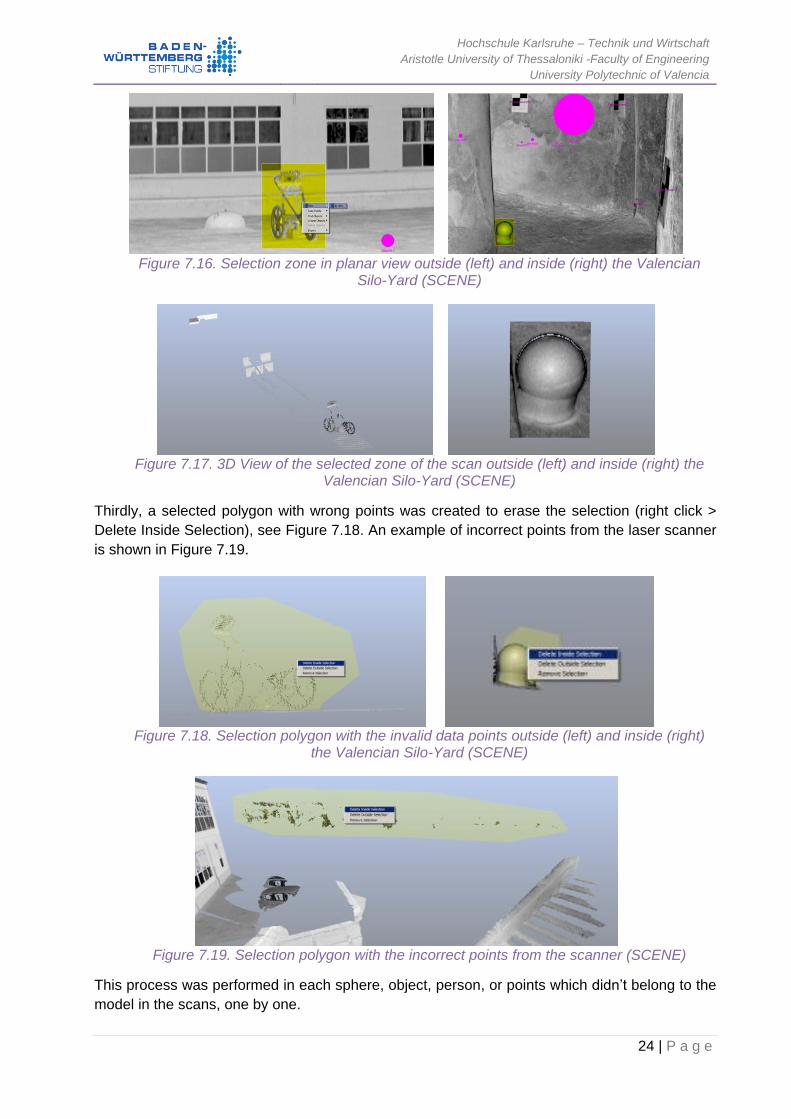
7.4.3. Estimation error after transformation
The tool “Distance computation” was used in order to obtain the estimation error that is the
distance between two clouds. To open this tool, in the top menu “Tools > Distance >
Cloud/Cloud Dist.”
In this case the reference cloud was from the UAV and the compared cloud was from the TLS,
the result obtained was 0.033 m of mean distance and a standard deviation of 0.024. These
results indicate that the aligned between both clouds was correct, see Figure 7.26. Therefore, it
was possible to continue with the georeferencing of the TLS scans.
Hochschule Karlsruhe – Technik und Wirtschaft
Aristotle University of Thessaloniki -Faculty of Engineering
University Polytechnic of Valencia
29 | P a g e
Figure 7.26. View of the TLS point cloud colorize by distance and histogram by approximate
distances (CloudCompare)
7.4.4. TLS Scans Georeferenced
After doing some test with different scans, it was necessary to move the scans one by one in
CloudCompare. The best way of applying the transformation matrix was loading the point
clouds which were used for the acquisition of the matrix, and then loading the scan to
georeference (exported from SCENE). As the coordinates of the point clouds were too large,
CloudCompare translated the data near the origin (0, 0). When the point cloud was loaded, the
tool that was executed was “Apply transformation” (this instrument is in the top menu “Edit >
Apply transformation (Ctrl+T)”), using the transformation matrix TLS to UAV (Figure 7.25).
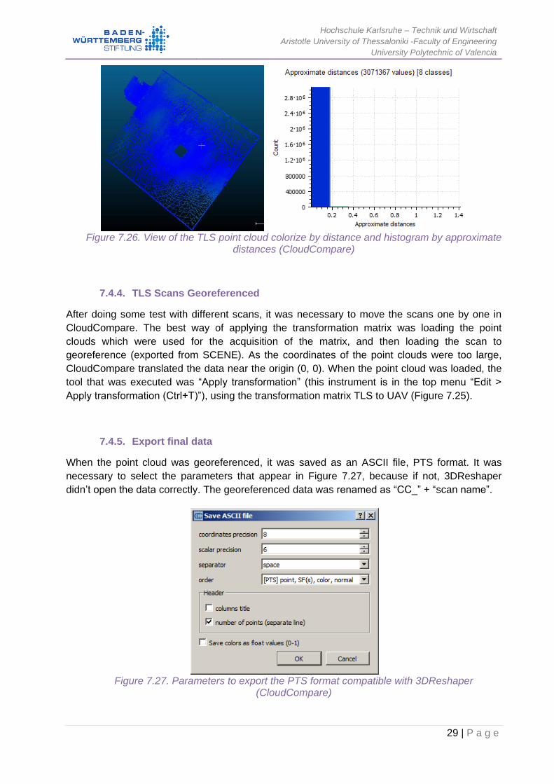
7.4.5. Export final data
When the point cloud was georeferenced, it was saved as an ASCII file, PTS format. It was
necessary to select the parameters that appear in Figure 7.27, because if not, 3DReshaper
didn’t open the data correctly. The georeferenced data was renamed as “CC_” + “scan name”.
Figure 7.27. Parameters to export the PTS format compatible with 3DReshaper
(CloudCompare)

Hochschule Karlsruhe – Technik und Wirtschaft
Aristotle University of Thessaloniki -Faculty of Engineering
University Polytechnic of Valencia
30 | P a g e
7.5. Processing with 3DReshaper to generate the 3D model
This section presents the 3D model processing in 3DReshaper software. The most important
task is cleaning the point clouds, creating the mesh and texturing the model.
7.5.1. Description of the 3DReshaper software
In this project the version used of 3DReshaper was 17.0.6.24515, version of April 28th, 2017.
3DReshaper is an easy-to-use dedicated to point cloud processing for various applications, like
Cultural Heritage, Architecture, Geology, Mine, Quarry, Digital Terrain Modeling, Civil
Engineering or Shipbuilding.
It includes a wide range of features, see Figure 7.28.
Figure 7.28. Range of features include in the software 3DReshaper (3D Reshaper 2015).
The following is a more detailed explanation of these features that we will use in this project.
These are Scripts, Point Clouds, 3D Meshes and Textures.
Scripts: (Scripting, JavaScript, Automation) In this project we will use this JavaScript environment to write own functions in order to
automate repetitive tasks. For instance, erase the noise, save the point cloud in different steps
of the process. Because if at any time it is necessary to compare with the old data, this is
possible.
3DReshape gives us some scripts and documentation free when we install the software or in
the web site in the download section. This information is inside of the program folder, it has a
file “Help for script” where you can find all information about the library of 3DReshaper. And
three folders: “Samples” with the project examples, “Script-Samples” and “Script-Tutorials” with
the code samples of some tasks usually made with 3DReshaper.
These custom commands can be run inside of 3DReshaper, also in silent mode if neither input
nor display is required, or with a dialog box containing parameters to set.

Hochschule Karlsruhe – Technik und Wirtschaft
Aristotle University of Thessaloniki -Faculty of Engineering
University Polytechnic of Valencia
31 | P a g e
Point Cloud Processing: (segmentation, noise detection, regular sampling, smart reduction) This module is a tool to process 3D point clouds, it is possible to import one or several point
clouds whatever their origin and size. The file formats supported by 3DReshaper can be seen in
the Table 7.3. The highlighted formats will be used in this project.
Table 7.3. File formats of Point Cloud supported by 3DReshaper (3D Reshaper 2015).
EXPORT IMPORT
ASCII FILES (*.asc / *.csv …)
Binary files (*.nsd)
Leica Geosystems (*.pts, *.ptx)
IGES (*.igs)
LAS (*.las)
AutoDesk DXF (*.dxf)
Fichiers ASCII (asc / csv / xyz / yxz– raw…)
Leica Geosystems (*.pts - .pcs - .pcst - .pcg - .pcsx -
.pcix - .pci - .pci - .ptx)
Leica Nova MS50 (*.sdb / *.xml)
ShapeGrabber (*.3pi)
STL file Binary (*.nsd)
Tool path (*.iso)
AutoDesk DXF (*.dxf)
STL (*.stl)
DMIS file (*.dms)
DMIS ASCII files - only the section "SET of POINT
(*.rmr)
GSCAN file (*.gsn)
Confocal Scanning Laser Microscope (*.csv)
NIKON Nexiv video measuring system (*.csv)
Perceptron SWB/SWL (*.swb / *.swl)
Polyworks (*.psl)
Leica T-Scan + Steinbichler (*.ac)
LIDAR data (*.las)
Autres ASCII (*.*)
Zoller and Fröhlich *(.zfs - *.zfc)
PLY points without triangles (*.ply)
ESRI ASCII (raster format *.asc)
FARO (*.fls - *.fws)
POLYWORKS (*.psl)
Coreview (*.atr / *.ftr)
E57 (*.E57 files)
LandXML files (*.xml)
The most important step in this project is to process or prepare the Point Cloud. These will be
implemented through noise detection, segmentation, regular sampling, smart reduction … in
order to save time with the subsequent step (meshing).
Some of the functions that provide 3DReshaper are for processing the point clouds. For
instance, it is possible to import point clouds without limit of the imported number of points.
There is “Clever reduction” to keep best points and remove points only where density is the
highest. Also exists “Automatic segmentation”, automatic or manual separation and cleaning,
“Density homogenization” for extract the best points evenly spaced, automatic “noise
measurement reduction”. Others tools allow change the colors according to a given direction.
Fusion. Registration, Alignment and Best Fit. It is possible to make a 3D comparison with a
mesh or a CAD model, Planar sections. 3DReshaper give the opportunity to representation in
several modes: textured, shaded, intensity (information depending on the imported data). These
are some of the most important tools of 3DReshaper for point clouds.

Hochschule Karlsruhe – Technik und Wirtschaft
Aristotle University of Thessaloniki -Faculty of Engineering
University Polytechnic of Valencia
32 | P a g e
3d Meshing: (3d Meshing, 3D Modeling, Ground Extraction, Mesh Improvement) This module is one of the most powerful, because the process of large point clouds obtains
light-weight, accurate and aesthetic models quickly.
The software provides different strategies to give the best meshing in accordance with the
quality of the original point cloud and the expectations that we want to obtain.
The software developers recommend in case of noisy point clouds two steps to be made to get
a perfect solution. In a first step, a very rough mesh is created in order to have quickly the
global shape. And in a second step, this rough mesh is refined with the point cloud by adding
triangles where we have the details.
Another suggestions or recommendations are using specific triangle reorganization. This
consists of meshing along curvatures is a 3DReshaper feature that enables to organize
triangles according to local curvature. The triangle reorganization follows the "flow" of the shape
so that sharp angles and small radii are better respected.
This powerful technique of "specific triangle reorganization" significantly improves the quality of
the 3D meshed models, with greater accuracy of the shape, especially in sharp angles and
small radius areas, with better aesthetics and smoothing of the shapes and lower number of
triangles needed to reach final tolerance of the model.
When the meshes are created, this software offers many tools to improve the mesh, for
example, the tool “Smoothing” to keep details but improve the general aspect, “Holes filling” is
used to treat a zone that could not be scanned or to obtain a closed model. The tool
“Decimation” is order to reduce the size of your meshes. The tool “Sharp Edges Reconstruction”
is to obtain perfect edges even if they are not scanned with a very high density. The tool
“Constraint Meshing” is to use a poly-line as a break-line in the mesh. These are some tool of
many others.
This software also has two other tools that are not used in this project but are important to know
that exist. One of these tools is “Ground Extractor” dedicated to creating a DTM. And another
tool is “Building Extractor” which is used to create simplified meshes.
The file formats supported by 3DReshaper can be seen in the Table 7.4.
Table 7.4. File formats of Mesh supported by 3DReshaper (3D Reshaper 2015).
EXPORT IMPORT
Ascii and binary STL format (*.stl)
Binary PBI format (*.pbi)
DXF 3Dface format (*.dxf)
Ascii POLY format (*.poly)
Vertices only (*.asc)
DXF polyline (*.dxf)
Universal IDEAS (*.unv)
OBJ formats (*.obj)
STEP file (*.stp)
Ascii Leica format (*.msh)
VRML 2 (*.wrl / *.vml / *.iv)
PLY (*.ply)
STL format (*.stl)
Binary PBI format (*.pbi)
DXF 3Dface format (*.dxf)
Ascii POLY format (*.poly)
OBJ format (*.obj)
Ascii Leica format (*.msh)
MDL format (*.mdl)
VRML files (*.wrl / *.vrml / *.iv)
OFF files (*.off)
PLY (*.ply)

Hochschule Karlsruhe – Technik und Wirtschaft
Aristotle University of Thessaloniki -Faculty of Engineering
University Polytechnic of Valencia
33 | P a g e
Camera & Textures: (Texture Mapping, Ortho-Photo, Mesh Coloration, Camera Calibration, Texture Atlas) This module is very important for obtaining a realistic product, because it is a manager to apply
textures on a mesh and a way to add details.
The software providers recommended three ways to map the texture. The fist way, it is use the
camera internal parameters (focal length or sensor size) and the external parameters (position
and orientation) to precede an automatic mapping. The second way, it is use couples of points
(point on the mesh and point on the picture) to compute automatically the camera parameters.
And the last way is use both some camera parameters and couples of points if some
information is missing. Also, it is possible to use ortho-photos or ortho-images to textured
meshes or exported through several formats (as OBJ or VRML) in order to be used in other
softwares.
This software also has three others functions: “Fully Automatic Texture Mapping”, “Camera
Calibration”, “Simply apply Color on Meshes”.
7.5.2. Merge data by zones
In order to optimize the work in this large-project, it was necessary to subdivide the heritage
area into seven big zones, see Figure 7.29. Also, some of these zones were subdivided again
to make the 3D model.
Figure 7.29. Schema about which scan belongs to each zone
The first zone alludes to the inside of the Silos, this was composed by scan numbers 002, 003,
005, 006, 007, 008, 009, 010, 011, 012, 013, 014, 015, 016, 017, 018, 019, 020, 021 and 022.
Some of these scans have color.
The rest of the zones allude outside of the Silos, the second zone was the north - east wall
which gave access inside of the silos. This zone was composed of the scans 021 - 031 and 057.
The third zone was the stairs which gave access to the Silos square, this was composed by the
scan numbers 023, 050 - 064. The fourth zone referred to the south - west wall, the scans of

Hochschule Karlsruhe – Technik und Wirtschaft
Aristotle University of Thessaloniki -Faculty of Engineering
University Polytechnic of Valencia
34 | P a g e
this wall had color, and the numbers of scans were from scan 042 until scan 050. The fifth zone
corresponds with the north - west wall, this zone was composed by scans number 038-042 and
065. The sixth zone corresponded with the building of the church, the numbers of the scans
were 030-041 and 065. And the last part was the seventh zone, which corresponded with the
Silos square, these numbers of scans were from the scan 066 up to the scan 073.
Finally, this project explains the 3D modeling inside the Silos, the diagram of the processes can
be seen in Figure 7.30. And outside the Silos, it was explained by another participant (Yepes
2017). In order to separate the project for each student, at this point the scans which had one
part inside and another outside were separated in two parts; these scans were
“CC_silos_Silos022” and “CC_silos_Silos021”. The obtained results were renamed as
“CC_silos_Silos022_inside”, “CC_silos_Silos022_outside”, “CC_silos_Silos021_inside” and
“CC_silos_Silos021_outside”.
This separate work was merged in the last part to visualize the complete Valencian Silo-Yard in
virtual reality.
Figure 7.30. Diagram of the processes in 3DReshaper
Process 0
(P0)
• Separate point clouds in silos and corridors
• Subdivide the silos and corridors into two parts
Process 1
(P1)
• Remove the electric installation
• Delete targets and some invalid points
Process 2
(P2)
• Filtering noise
Process 3
(P3)
• Create mesh
• Refine mesh with point cloud
Process 4
(P4)
• Smooth mesh
Process 5
(P5)
• Clorize the mesh with the cloud points
• Or texturize the mesh with the images of Agisoft PhotoScan
Process 6
(P6)
• Merge meshes, reduce meshes
• Translate mesh and export it

Hochschule Karlsruhe – Technik und Wirtschaft
Aristotle University of Thessaloniki -Faculty of Engineering
University Polytechnic of Valencia
35 | P a g e
7.5.3. Subdivide the point clouds in Silos and corridors (P0)
At the beginning, the noise reduction was tested, but the points which appeared in pink (Figure
7.31) in the preview will be deleted. At that moment, the process was not applicable, because
these points defined the corridor. The same situation happened in other scans. Therefore, the
filter noise will be applied later, once the clouds will be combined and separated by corridors
and silos, and the illumination deleted.
Figure 7.31. Filter clouds, noise reduction (3DReshaper 17.0.6.24515)
Seven corridors and six silos that composed the study are inside the Valencian Silo-Yard, all the
interior scans were measured in high resolution. The silos and corridors are catalogued in the
scheme of the Figure 7.32.
Figure 7.32. Schema of the location and numbering of each silo and corridor (orthophoto
(Soubry 2016))
The methodology to subdivide the point clouds in 3DReshaper is described below. This process
was done in every silo and corridor, one by one. It consisted of separating out the point clouds,
afterward grouping parts of point clouds in a cloud and renaming this point cloud.
Firstly, it was necessary to load all the scans that had some data of this corridor or this Silos,
(3D > Import > Point Cloud). Secondly, all point clouds were selected, then it was to click on the
“Clear / Separate Cloud(s)” tool (this instrument is in the top menu, Cloud > Clean / Separate
Cloud(s) > Keep the two parts), and the points were inserted around the corridor or silo to

Hochschule Karlsruhe – Technik und Wirtschaft
Aristotle University of Thessaloniki -Faculty of Engineering
University Polytechnic of Valencia
36 | P a g e
separate them from the others clouds. Each selected cloud was painted in a different color,
these fragments of clouds were very important to complete the corridors (Figure 7.33).
Figure 7.33. Selected cloud to separate Corridor_01 (left) and Silo_01 (right) (3DReshaper)
Thirdly, some noise was erased which was not detected in SCENE. This process was done
before merging the clouds, because it was easier to eliminate noise from a scan. Some
examples can be seen in Figure 7.34.
Figure 7.34. Example of noise elimination in 3DReshaper (3DReshaper)
Finally, the separated clouds were selected and then executing the “Merge Clouds” tool (this
instrument is in the top menu, Cloud > Merge Clouds), see in Figure 7.35. Then the combined
cloud was renamed following the nomenclature of the Figure 7.32.
Figure 7.35. Selected clouds to merge in a cloud “Corridor_01” (3DReshaper)
The 3D model inside the building was not done, because there were not sufficient scans in this
area and this part was not very important (Figure 7.36).

Hochschule Karlsruhe – Technik und Wirtschaft
Aristotle University of Thessaloniki -Faculty of Engineering
University Polytechnic of Valencia
37 | P a g e
Figure 7.36. Scans inside of the building (3DReshaper)
When all the clouds were classified between corridors and silos, it was the moment to erase the
electrical installation and the targets. Due to the morphology of the Silo, this one was measured
from the interior. Therefore, some planes were created to divide the silos in two parts to see
inside.
7.5.3.1. Separate the silo into two parts
The methodology to separate the silo into two parts in 3DReshaper is described below. Firstly, it
was necessary to create the plane into the Silo (the tool is in the top menu, Construct > Plane >
Plane / Draw). In order to do the plane perpendicular, it was necessary to inset zero in the z
axis, which fixed the normal and in the z axis which fixed the second axis. A plane was created
in each silo, see Figure 7.37.
Figure 7.37. Planes perpendicular to every silo (3DReshaper)
Secondly, the silo cloud and its plane was selected and then the “Separate with object” tool was
executed (this instrument is in the top menu, Cloud > Separate with object). Finally, the two
clouds obtained for each silo was renamed with the name of the cloud + “_1” or “_2”. This
process was performed for each Silo.

Hochschule Karlsruhe – Technik und Wirtschaft
Aristotle University of Thessaloniki -Faculty of Engineering
University Polytechnic of Valencia
38 | P a g e
7.5.3.2. Separate the corridor into two parts
Also, the corridors were separated, but the “Clear / Separate Cloud(s)” tool was executed (this
instrument is in the top menu, Cloud > Clean / Separate Cloud(s) > Keep the two parts), see
Figure 7.38 . Finally, the two clouds obtained for each corridor were renamed with the name of
the cloud + “_1” or “_2”. This process was performed for every corridor.
Figure 7.38. Separating the corridor into two parts (3DReshaper)
7.5.4. Delete the electrical installation and targets (P1)
This process of separating the electrical installation and targets of the point cloud was the most
important step to obtain a correct 3D model.
Depending on the point cloud, it was sometimes possible to use the data segmentation to
separate the electrical installation, but in other cases this was not useful. Both methods are
explained below. An example of the electrical installation and the target to be cleaned can be
seen in Figure 7.39.
Figure 7.39. Example of the electrical installation and targets to be deleted (3DReshaper)
7.5.4.1. Data segmentation for deleting the electrical installation
The following is a description of the methodology to delete the electrical installation through the
data segmentation in silos and corridors. Firstly, it was necessary to load half -silo point cloud or
half -corridor point cloud, (3D > Import > Point Cloud). It was selected and afterwards the “Filter
/ Explode Cloud(s)” tool was executed (this instrument is in the top menu, Cloud > Filter /
Explode Cloud(s) > Explode with distance). With this tool, it was necessary to change the value

Hochschule Karlsruhe – Technik und Wirtschaft
Aristotle University of Thessaloniki -Faculty of Engineering
University Polytechnic of Valencia
39 | P a g e
of the distance and check the preview to obtain the result expected (Figure 7.40). The different
colors will be separated into different point clouds.
Figure 7.40. Data segmentation with default value (3DReshaper)
Due to the result of Figure 7.40, it was not possible to apply the segmentation to a half -silo.
Therefore, the part around the electrical installation was extracted and then the segmentation
was applied to this fragment (Figure 7.41). In this case, the optimal result was obtained using
5mm in the segmentation distance.
Figure 7.41. Fragment segmentation 5mm (3DReshaper)
Secondly, all point clouds that belong to the wall were merged into a point cloud. And the other
point clouds that belong to the electrical installation were merged into another point cloud
(Figure 7.42). Usually, some parts of the electrical installation appeared on the wall cloud. In
order to delete these parts it was possible to use another segmentation or to manually separate
these parts (Cloud > Clean / Separate Cloud(s) > Keep the two parts).
Figure 7.42. First point cloud of wall (left) and first point cloud of electrical installation (right) (3DReshaper)
Finally, when the electrical installation was separated from the fragment of the point cloud, this
fragment was combined with the half -silo or half –corridor and renamed like “p1_”+ cloud name.
This process was realized for each half -silo and each half -corridor.

Hochschule Karlsruhe – Technik und Wirtschaft
Aristotle University of Thessaloniki -Faculty of Engineering
University Polytechnic of Valencia
40 | P a g e
7.5.4.2. Delete the electrical installation without segmentation
The obtained results of the segmentation of point clouds sometimes were not useful to separate
the electrical installation (Figure 7.43). Therefore, in these cases, the electrical installation was
separated by hand.
Figure 7.43. Non-optimal segmentation (3DReshaper)
The methodology to separate manually the electrical installation is described below. Firstly, the
half of the point cloud was selected and the “Clear / Separate Cloud(s)” tool was executed, later
points were inserted around the object to separate it (Figure 7.44). As soon as the electrical
installation was separated, the final step was the same that the final step of data segmentation.
Figure 7.44. Manually separating of electrical installation (3DReshaper)
7.5.4.3. Delete targets
The following is a description of the methodology to remove manually the parts of the targets in
the half -silos and in the half –corridors due to the fact that some targets were changing the
morphology of the silo or the corridor, because these targets were not completely pasted to the
wall. This process was very similar to the manual separation of the electrical installation. The
“Clear / Separate Cloud(s)” tool was used only to separate the parts which were not preserving
the geometry of the silo wall (Figure 7.45), it was performed for every target.
Figure 7.45. Process of removing parts of the targets (3DReshaper)
The points that are conserved of the target were used to generate the 3D model, but not to give
the color to the model on the place that did not have photos.

Hochschule Karlsruhe – Technik und Wirtschaft
Aristotle University of Thessaloniki -Faculty of Engineering
University Polytechnic of Valencia
41 | P a g e
7.5.4.4. Delete points in some zones
Sometimes, the mistake of overlapping was taking place when the different scans were
superposed. For example, the overlap error appears on the stairs, this can be seen in Figure
7.46, which was deleted to avoid the noise in the mesh.
Figure 7.46. Delete noise from the stairs (3DReshaper)
The atypical case also occurs in the stairs (Corridor_07), due to a plastic cover or something
similar that covers the ruined wall. The Laser Scanner could measure the wall behind the plastic
cover, but also some parts of the plastic cover. These wrong points were very difficult to erase,
see Figure 7.47.
Figure 7.47. RGB picture of the plastic cover (Valenciabonita 2017), before to deleting the
noise (left), and deleting the noise of the plastic cover (right) (3DReshaper)
7.5.5. Automatically filter data noise (P2)
The noise filtering process was performed, when the electrical installation and targets were
deleted. This process deleted some random noise points, and also the intensity was chosen to
be applied.
The following describes the methodology to filter the noise of the point cloud obtained in the
previous process (Process 1 - Delete the electrical installation and targets) in 3DReshaper.
Firstly, the scans with half -corridor or half -silo were loaded, (3D > Import > Point Cloud).
Afterwards, the point cloud was selected and the “Noise reduction” tool was executed (this
instrument is in the top menu, Cloud > Filter / Explode Cloud(s) > Noise reduction), the
“intensity 0” was normally used (Figure 7.48), because otherwise, the points which had no noise
were deleted. Usually, this process was executed in three iterations. For each iteration, it
sometimes deleted around a maximum of 0.1% of the total number of points. In some cases,
this percentage might be higher, it revised that the points to delete of blue color were noise
points. This process was done for each half -corridor and each half -silo, which was renamed as
“p2_”+ cloud name.

Hochschule Karlsruhe – Technik und Wirtschaft
Aristotle University of Thessaloniki -Faculty of Engineering
University Polytechnic of Valencia
42 | P a g e
Figure 7.48. Noise reduction iteration 1, points to delete (blue) (3DReshaper)
Secondly, every half -cloud was merged with the other half -cloud in the same zone. Both point
clouds were selected, afterwards the “Merged Clouds” tool was executed (this instrument is in
the top menu, Cloud > Merged Clouds). Then, the noise reduction was applied once again and
it was renamed as “p2_”+ cloud name of the zone+ “_3”.
7.5.6. Create 3D mesh (P3)
In order to create a realistic 3D mesh, it was created in two steps. The first step was creating a
gross 3D mesh without details to fill the holes, and the second step was creating a refined mesh
to visualize the bricks and details on the walls. The following is a description of the methodology
of the 3D mesh creation of silos and corridors of the last process (Process 2 - Automatically
filter data noise).
Firstly, the point cloud was selected and the “3D mesh” tool was executed, (the instrument is in
the top menu, Mesh > 3D Mesh). Normally, in this step it is appropriate to use approximately
three centimeters, this means that the mesh had a 3 cm of precision.
Secondly, the 3D mesh was checked, sometimes it was necessary to fill some small holes. In
order to do this, the mesh was selected and then the “Fill holes” tool was executed, (the
instrument is in the top menu, Mesh > Fill holes), see Figure 7.49.
Figure 7.49. Filled holes before (left) and after (right) (3DReshaper)
Thirdly, when all holes were filled, it was time to refine the mesh with the corresponding point
cloud obtained in the process 2 (P2). The mesh and the point cloud were selected and then the
“Refine Mesh / From a point cloud” tool was executed (this instrument is in the top menu, Mesh
> Refine Mesh > From a point cloud). Normally the mesh was refined to three millimeters

Hochschule Karlsruhe – Technik und Wirtschaft
Aristotle University of Thessaloniki -Faculty of Engineering
University Polytechnic of Valencia
43 | P a g e
(Figure 7.50), this means that the model had a 3 mm of precision. Only in the “Silo_02” was
refined to 1 mm to see the bricks in the model. In this step the 3D mesh was improved.
Figure 7.50. Refined mesh to 3mm before (left) and after (right) (3DReshaper)
Fourthly, once the 3D mesh was checked, sometimes it was necessary to eliminate some
spikes. To do this, the mesh was selected and then the “Eliminate Spikes” tool was executed,
(the instrument is in the top menu, Mesh > Eliminate Spikes). Finally, the obtained mesh was
renamed with “p3_”+cloud name of the zone. This process was performed for each silo and
each corridor.
7.5.7. Smooth the mesh (P4)
The next step was to smooth the mesh, which was obtained from the last process (Process 3 -
Create 3D mesh). In order to smooth the mesh, it was selected and the “Regular Smoothing”
tool was executed, (the instrument is in the top menu, Mesh > Smooth mesh > Regular
Smoothing). Normally, in this step the “keep details” property was used in the mesh in order not
to lose detail. Finally, the mesh obtained was renamed with “p4_”+ cloud name of the zone, for
example, “p4_Silo_03.ply”. This process was performed for every silo and corridor.
7.5.8. Colorize or texturing the mesh (P5)
The following is a description of how the silos meshes and corridors meshes of the last process
(Process 4 - Smooth the mesh) were colorized. Some samples of a silo with different textures
can be seen in the Table 7.5. The texture of the 3D mesh was applied through two different
methodologies (using color images or color of the Laser Scanner), with different results.
Table 7.5. Sample of a 3D silo model but with different textures (3DReshaper)
A. Without
texture
(Obtained in the
process 4)

Hochschule Karlsruhe – Technik und Wirtschaft
Aristotle University of Thessaloniki -Faculty of Engineering
University Polytechnic of Valencia
44 | P a g e
B. Texture with
intensity value of
the Scanner
C. Texture with
Scanner color
D. Texture with
orthomosaic
(only available in
3 of 6 Silos),
obtained with
Agisoft
PhotoScan
With the intensity value of the Scanner, the corridors meshes were colored, because in the
measurements the color was not taken. The texture with the color of the Scanner was used to
color the silos meshes, where they were not photographed. And the texture with the ortho-
mosaic obtained with Agisoft PhotoScan was used to texture the first three silos of the entrance.
The methodology of these options is explained below.
7.5.8.1. Colorize the mesh
This process was used in corridors and silos without images. To color the mesh, it was selected
and the “Take Color form Cloud” tool was executed, (the instrument is in the top menu, Mesh >
Take Color from Cloud), (Table 7.5 – B, Table 7.5 – C,). Normally, in areas where there were no
color points, the average color was taken from the closest points. Also, it was possible to
choose the distance and the default color to paint the mesh when that distance was exceeded.
Finally, the mesh obtained was renamed with “p5_”+ cloud name of the zone. This process was
performed for each silo and each corridor. This mesh was exported in PLY format, in order to
store the colored mesh.

Hochschule Karlsruhe – Technik und Wirtschaft
Aristotle University of Thessaloniki -Faculty of Engineering
University Polytechnic of Valencia
45 | P a g e
7.5.8.2. Texturing the mesh
This process was used in the first three silos from the street access, in these silos there were
images and thermal images. In this method, mosaics were used (Figure 7.51) from Agisoft
PhotoScan generated with normal images. It is explained in the next chapter.
Figure 7.51. Mosaics of Silo_01
The methodology to texture the mesh is described below. Firstly, the mesh was selected and
afterwards the “Texture From Pictures - From Reference Points” tool was executed (the
instrument is in the top menu, Image > Texture From Pictures > From Reference Points). It was
very difficult to insert the reference points, due to, there were no regular objects as windows in
this place. The point cloud was used to place the reference points, see Figure 7.52. When the
image was fixed in the mesh, the reference points were exported into a TXT file with the name
of the image and the silo, this file will be necessary later.
Figure 7.52. Insert reference points to texturing the mesh (3DReshaper)
Secondly, the images were edited in Photoshop software to eliminate the targets and the
electrical installation, as these objects were not in the mesh. Thirdly, the new images modified
in Photoshop and the reference points of every image were imported. Since the images had the
same dimension as the images used in the first step, all the images were located in the correct
place.

Hochschule Karlsruhe – Technik und Wirtschaft
Aristotle University of Thessaloniki -Faculty of Engineering
University Polytechnic of Valencia
46 | P a g e
Fourthly, in this software we had the opportunity to choose manually which triangle was texture
by each image, this allowed to give a realistic result. The mesh was selected, afterwards the
“Adjust Textures” tool was executed (this instrument is in the top menu, Image > Adjust
Textures), see Figure 7.53.
Figure 7.53. Adjusting the textures in the silo (3DReshaper)
Finally, the mesh obtained was renamed with “p5_” + cloud name of the zone. This process was
performed only in the first three silos. This mesh was exported in OBJ format which stored the
mesh and the images that were used to texturing the mesh.
7.5.9. Merging all the meshes
The following is a description of the methodology for combining all meshes in one mesh. The
“Merge Common Borders” tool was executed, as it was not maintaining the color of the mesh,
the topology was recreated to combine common boundaries, due to this, it was necessary to
use another tool. To do this, the two meshes were selected and the “Join 2 Contours” tool was
executed (this tool is in the top menu, Mesh > Join 2 Contours), this tool joined two meshes on
a surface, see Figure 7.54. This process was necessary to avoid holes between silos and
corridors.
Figure 7.54. Joined two mesh (3DReshaper)

Hochschule Karlsruhe – Technik und Wirtschaft
Aristotle University of Thessaloniki -Faculty of Engineering
University Polytechnic of Valencia
47 | P a g e
7.5.10. Reduced mesh
The goal to reduce the mesh was that the model was represented by fewer triangles, but with
the same range of quality. This was achieved so that the software could run more rapid and
storage less space on the disc. Depending on the purpose of the model it was possible to be
reduced more or less. In other words, the model could maintain more or less detail, but for the
cultural heritage aim it was necessary to have high resolution. For example, in the plane
surfaces not so many triangles were necessary.
In this case the morphology of the silos and the corridors had the same characteristics, for this
reason the reduction was applied to the fused mesh. To do this, the mesh was selected and the
“Reduce” tool was executed (this instrument is in the top menu, Mesh > Reduce). In order to
analyze if this reduction had many changes in the model, it was necessary to check the model
with the next tool, so that the original mesh and the reduced mesh was selected, afterwards the
“Compare / Inspect” tool was executed (this instrument is in the top menu, Measure > Compare
/ Inspect). Some samples with different deviation values can be seen in Table 7.6, the first
reduction of Table 7.6, the reduction ratio was very high, but it was not appropriate in this case
because all details disappeared. In this project, it was very important to conserve the bricks or
other details. Therefore, between the second and third reduction the reduction rate was similar,
the third reduction was chosen, maximal deviation of 1 mm, because the model was not
distorted and the morphology of the silos and corridors was maintained.
Table 7.6. Samples of different grade of reduction (3DReshaper)
A. Information
about the first
reduction
Average deviation: 0.00380 m
Maximal deviation: 0.01000 m
Reduction rate: 98.4%
B. Information
about the
second
reduction
Average deviation: 0.00074 m
Maximal deviation: 0.00300 m
Reduction rate: 68.3%
C. Information
about the third
reduction
Average deviation: 0.00048 m
Maximal deviation: 0.00100 m
Reduction rate: 65.8%
The characteristic of the reduction chosen (Table 7.6 – C.) had a maximal deviation of 1 mm,
and the reduction rate is 65.8% respect of the original mesh, more than 90% of the surface
changes its position less than 1 mm. Looking at the Figure 7.55, the maximal change in the
reduced mesh with regard to the original mesh was 3.7 mm in less than 0.01% of the total

Hochschule Karlsruhe – Technik und Wirtschaft
Aristotle University of Thessaloniki -Faculty of Engineering
University Polytechnic of Valencia
48 | P a g e
surface. The original mesh had about three million triangles and the reduced mesh to 1 mm had
about one million triangles, the difference in the number of triangles was high, the model was
reduced two million triangles. This reduction was very important.
Figure 7.55. Comparing between the original mesh and the reduced mesh 1mm
(3DReshaper)
Then, the first three silos were separated, as the RGB or thermal texture was changed. These
silos were separated in this step, since the clean cut between the silos and corridors was
perfect. There were no holes when the texture was changed, see Figure 7.56. These silos were
colored with the texture, the process can be seen in section “7.5.8.2 Texturing the mesh”.
Figure 7.56. Separate the first three silos of the reduced mesh of 1 mm (3DReshaper)
7.5.11. Translated mesh
When all the processes were done, it was time to apply the translation to the model. To do this,
the final meshes were selected and the “Translation” tool was used (this instrument is in the top
menu, Construct > Translation), in order to create a new object translated.
Figure 7.57. Translated mesh (3DReshaper)

Hochschule Karlsruhe – Technik und Wirtschaft
Aristotle University of Thessaloniki -Faculty of Engineering
University Polytechnic of Valencia
49 | P a g e
In order to know the distance to be translated, it was consulted on the official website of the
Valencian community (ICV – Terrasit), to obtain the coordinates of the point where the
coordinate origin was near the Valencian Silo-Yard. Therefore, the translated values were “-
722430 m” in North and “- 4376410 m” in East, this translation was done not to have problems
when using this data in another software and not 3DReshaper, because another software
cannot open the project in the original coordinates.
The colored meshes were exported to the PLY format, and the textured meshes were exported
to the OBJ format. In addition, with this program, it was possible to obtain the volume of the
meshes, whichcan be seen in “Appendix I”.
7.5.12. Scripts with 3DReshaper
The programming in JavaScript language was used with the “Script > Run” tool, the example of
the code can be seen in Table 7.7. This script was developed to save the loaded point clouds in
the 3DReshaper software (“.rsh”).
Table 7.7. Script to save the point clouds (3DReshaper)
p0_Save_Clouds_load_in_rsh.js
// Set the current directory to our containing folder
var curDir = CurrentScriptPath();
print(curDir);
// Load all the clouds of the rsh file
var clouds = SCloud.All(2);
print('clouds: '+clouds);
for( var num_cloud=0 ; num_cloud < clouds.length ; num_cloud++){
cloud = clouds[num_cloud];
print('nube: '+cloud);
var name =cloud.GetName();
var res = cloud.Save(curDir+'/save/'+name+'.pts');
if (res.ErrorCode != 0)
throw new Error('Save cloud failed : '+num_cloud);
}
print('Finished, save cloud.');
7.5.13. Some problems or errors detected
7.5.13.1. Errors in Scanner measurements
In the measurements that were taken inside the silos, there was some error in the upper part,
due to this the Laser Scanner measured twice the same zone. The points were very close to
each other but in a different position. Therefore, it made noise in the model. The problem can be
seen in Figure 7.58. To do this, one of the repeated parts was deleted manually so that no noise
appears in the model. The erasing process can be seen in Figure 7.59.
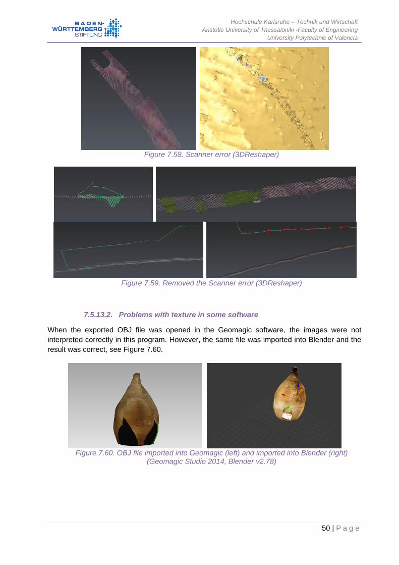
Hochschule Karlsruhe – Technik und Wirtschaft
Aristotle University of Thessaloniki -Faculty of Engineering
University Polytechnic of Valencia
50 | P a g e
Figure 7.58. Scanner error (3DReshaper)
Figure 7.59. Removed the Scanner error (3DReshaper)
7.5.13.2. Problems with texture in some software
When the exported OBJ file was opened in the Geomagic software, the images were not
interpreted correctly in this program. However, the same file was imported into Blender and the
result was correct, see Figure 7.60.
Figure 7.60. OBJ file imported into Geomagic (left) and imported into Blender (right)
(Geomagic Studio 2014, Blender v2.78)

Hochschule Karlsruhe – Technik und Wirtschaft
Aristotle University of Thessaloniki -Faculty of Engineering
University Polytechnic of Valencia
51 | P a g e
7.6. Processing with Agisoft PhotoScan to create the texture
This section presents the image processing in Agisoft PhotoScan software. The most important
task is to create the orthomosaics with the RGB images and to texture the model with the
thermal images.
7.6.1. Description of the Agisoft PhotoScan
In this project the version that we use is Agisoft PhotoScan, version 1.2.6.2834.
Agisoft PhotoScan is a photogrammetric image processing product and generates 3D spatial
data. Mainly this software is used for documentation of cultural heritage and GIS applications
(Agisoft 2017).
7.6.2. Generated the orthomosaic in RGB
In order to generate the interior texture of the silos it was necessary to follow the steps of the
Table 7.8.
Table 7.8. Process of generating the interior texture in RGB (Agisoft PhotoScan)
1. Add the Photos
2. Align the photos, where the “pair preselection” was chosen “generic”, the paired search of points before and after the image was not used.
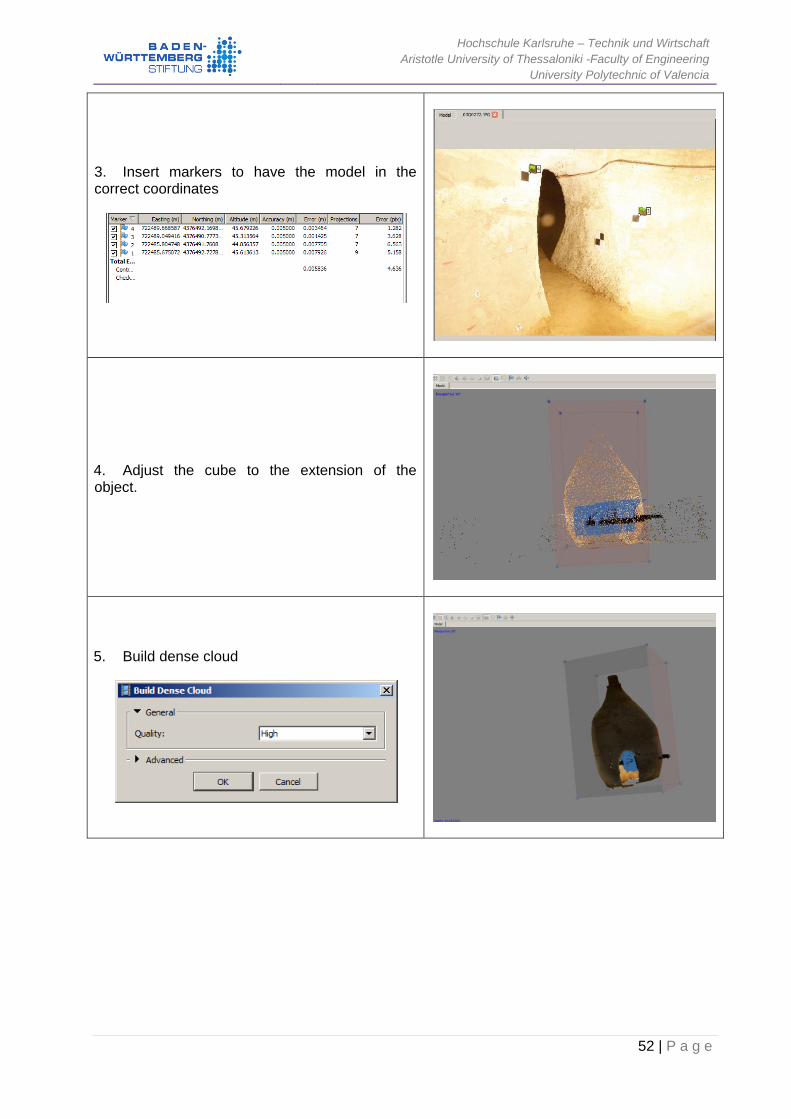
Hochschule Karlsruhe – Technik und Wirtschaft
Aristotle University of Thessaloniki -Faculty of Engineering
University Polytechnic of Valencia
52 | P a g e
3. Insert markers to have the model in the correct coordinates
4. Adjust the cube to the extension of the object.
5. Build dense cloud

Hochschule Karlsruhe – Technik und Wirtschaft
Aristotle University of Thessaloniki -Faculty of Engineering
University Polytechnic of Valencia
53 | P a g e
6. Build the mesh, in this case it was necessary to use the surface type as “Arbitrary”, because it was not a DEM (Digital elevation model)
7. Build orthomosaic, the projection plane to be exported were:
- Top XY - Front XZ - Back XZ - Right YZ - Left YZ - Bottom XY
8. Export orthomosaic
As soon as some orthomosaics had some wrong parts, some pictures were turned off and then
recreated (Figure 7.61)

Hochschule Karlsruhe – Technik und Wirtschaft
Aristotle University of Thessaloniki -Faculty of Engineering
University Polytechnic of Valencia
54 | P a g e
Figure 7.61. Dazzled image (left) and corrected image (right) (Photoshop)
This exported orthomosaic was used in 3Dreshaper to import this texture to the mesh. This data
was used in the section “7.5.8.2. Texturing the mesh”.
7.6.3. Applied the thermal images to the 3D model
These thermal images were not modified with Photoshop to remove the targets and the
electrical installation. In this case, the thermal texture was applied to the mesh in PhotoScan.
This process is described below for each silo.
7.6.3.1. Thermal texture of Silo 01 and Silo03
Since these images did not have a good resolution and quality, also they were taken half-silo
and then the other half-silo in “Silo_01”. The software didn’t recognize well the correspondence
between images, because the photographs were not taken in continuous circles. It only
recognized similarities between some images, this can be seen in Figure 7.62.
Figure 7.62. Aligned photos of the thermal images of “Silo_01” (Agisoft PhotoScan)
Then, the model obtained from 3DReshaper (Tools > Import > Import Mesh) was imported,
once it was loaded, afterwards the texture was created to see which images were not appearing
in the texture. In order to complete the model, new marks were assigned and only these photos
were realigned. Finally, the thermal texture of the model from 3DReshaper was created and can
be seen in Figure 7.63.

Hochschule Karlsruhe – Technik und Wirtschaft
Aristotle University of Thessaloniki -Faculty of Engineering
University Polytechnic of Valencia
55 | P a g e
Figure 7.63. Creating the final thermal texture of the 3DReshaper model (Agisoft
PhotoScan)
In the last step, the model was exported with the texture in OBJ format (File > Export model).
Then, the model was compared in 3DReshaper with the original mesh to see that its geometry
was not modified, see Figure 7.64.
Figure 7.64. Comparison of the original mesh with the PhotoScan texture mesh
(3DReshaper)
7.6.3.2. Thermal texture of Silo 02
There was no access to the images of “Silo 02” to do the same process of that in the previous
section. Nevertheless, we had access to the final data of last year, using the last year’s thermal
model created by Carbonell obtained from the model used in Unity software by Hadabay.
Then this model of the silo was imported into 3DReshaper to create the orthomosaic of the
same views that was obtained in PhotoScan. Finally, these images were applied as in the
section “7.5.8.2. Texturing the mesh”.

Hochschule Karlsruhe – Technik und Wirtschaft
Aristotle University of Thessaloniki -Faculty of Engineering
University Polytechnic of Valencia
56 | P a g e
7.7. Processing with Blender to create the virtual reality
This section presents the processing in Blender software. The most important task was to
compact the images used by a 3D model in an image and create the virtual reality.
7.7.1. Description of the Blender software
Blender is free and open source software, as a community-driven project under the GNU
General Public License (GPL). It is a cross-platform and runs equally well on Linux, Windows,
and Macintosh computers.
Blender supports the entirety of the 3D pipeline—modeling, rigging, animation, simulation,
rendering, compositing and motion tracking, even video editing and game creation. This
software also has Bender’s API for scripting to customize the application and write the
specialized tools.
The following is a more detailed explanation of the modules that can be used in Blender if there
is sufficient time in this work.
Camera and Object tracking With this module the aim is to create an animation to show the 3D modeling of the Valencian
Silo-Yard resulting from the 3DReshaper software.
This module includes auto and manual tracking of the camera and object, a powerful camera
reconstruction and a real-time preview of the tracked footage and 3D scene.
Game Creation This module is included in Blender, it is a complete game engine, it allows to create a fully
featured 3D game right inside Blender.
This module includes for example, theability to port the models to any third-party game engine.
It is possible to create or code with own game logic, also Python scripting API for advanced
control and AI. It is supported for all OpenGLTM dynamic lighting, toon shading, animated
materials as well as Normal and Parallax Mapping. It is allowed to playback games inside
Blender without compiling or preprocessing 3D spatial audio using OpenAL.
7.7.2. Compacting the images of a 3D model
The 3D models exported from 3DReshaper of the first three silos with RGB texture, exported
their six images with every model, so when trying to import this data into the virtual reality these
images of the meshes were very big.
The solution to this problem was to process this data with Blender and unify all the images to
one image per model. The tool that was used was “Object UV Editing”, this tool allowed
integrating all the images in one image. Firstly, the mesh was imported in OBJ format, when all
sub-meshes were selected. Then click “MultiObject UV Editing” (Tool > MultiObject UV Editing),
to edit the UV (these are the coordinates that assign to each vertex of the model, the value of
the texture) of the sub-meshes at the same time. Secondly, a new UVMap was created and the

Hochschule Karlsruhe – Technik und Wirtschaft
Aristotle University of Thessaloniki -Faculty of Engineering
University Polytechnic of Valencia
57 | P a g e
“Smart UV Project” (Mesh > Unwrap > Smart UV Project) was executed, which can be seen in
Figure 7.65.
Figure 7.65. “Smart UV project” executed (Blender 2.78)
Thirdly, at the time of assigning the texture to the mesh, a new image with the resolution was
created (Figure 7.66, left) to generate the texture there. In the case of the silos 4096 x 4096
pixels were used, see Figure 7.66. Then, the “Bake” button was clicked to bake the image with
the texture of the selected objects. The result can be seen in Figure 7.67.
Figure 7.66. Recommended resolution values (left) and creation of the new image (right)
(Blender)
Figure 7.67. Baked texture of the “Silo_01” (Blender)

Hochschule Karlsruhe – Technik und Wirtschaft
Aristotle University of Thessaloniki -Faculty of Engineering
University Polytechnic of Valencia
58 | P a g e
Fourthly, when the texture was created, all sub-meshes were joined (Ctrl + j), the old UVMap
and the old textures were deleted. Subsequently, the new image was loaded and assigned the
new UVMap, see Figure 7.68.
Figure 7.68. Assigning the new texture of an image (Blender)
This process was performed with all meshes that were included in the virtual reality (inside the
silos and also outside the silos with the results of Yepes (2017) where more than one image
was used in the texturing process. Sometimes, it was necessary to apply a rotation of -90º in x
with the OBJ format for the correct visualization in Blender.
7.7.3. Create virtual reality
The most important thing was the object that travels on the 3D model. The camera (1,5 meters
from the floor) and the light was associated with the cube, the objects were selected and clicked
on “Object > Parent > Object > Set Parent to Object”. It is not able to cross the walls (Physics
type > Dynamic), the parameters can be seen in Figure 7.69. With this process the children of
the cube are the camera and the light, in other words, when the cube moves the children also
move.
Figure 7.69. Cube parent with the camera and the light as children (Blender)

Hochschule Karlsruhe – Technik und Wirtschaft
Aristotle University of Thessaloniki -Faculty of Engineering
University Polytechnic of Valencia
59 | P a g e
This object can be moved with the mouse and the arrows, the game logic of the cube can be
seen in Figure 7.70. The movements were:
o Move proceed: up arrow o Move back: down arrow o Turn left: left arrow or move mouse o Turn right: right arrow or move mouse o Movement of the view: move mouse o Jump: right-click mouse
Figure 7.70. Game logic of the cube (camera) (Blender)
The texture in the first three silos (“Silo_01”, “Silo_02”, “Silo_03”) can be chosen pressing some
keys: (the logic game can be seen in Figure 7.71)
o If you press the number “1” key on the keyboard: The color to visualize is the color mesh (the color of the laser scanner colors the mesh)
o If you press the number “2” key on the keyboard: The texture to visualize is the real texture – realistic color (normal camera color)
o If you press the number “3” key on the keyboard: The texture to visualize is the thermal texture (color of thermal pictures with thermal camera)
Figure 7.71. Silos color game logic by pressing the number “1” (Blender)

Hochschule Karlsruhe – Technik und Wirtschaft
Aristotle University of Thessaloniki -Faculty of Engineering
University Polytechnic of Valencia
60 | P a g e
The efficiency of the virtual reality with the silos was very good, the frame-time was around 16.7
ms can be seen in Figure 7.72.
Figure 7.72. Efficiency of the virtual reality of the silos (Blender)
7.7.4. Export final data
In order to export the final virtual reality of the Valencian Silo-Yard with the model inside and
outside of the silos. It was necessary to activate the Add-ons “Save As Game Engine Runtime”.
Then, it was clicked File > Export > Game Engine Runtime. This tool generated all the files
necessary to open the virtual reality on any computer. It depends on the characteristics of the
computer if the game may take a little longer to start the virtual reality. The final result integrated
in the virtual reality of Blender can be understood in Figure 7.73.
Figure 7.73. Explicative diagram of the emplacement of the silos in the Valencian Silo-Yard

Hochschule Karlsruhe – Technik und Wirtschaft
Aristotle University of Thessaloniki -Faculty of Engineering
University Polytechnic of Valencia
61 | P a g e
7.7.5. The game’s instructions
In order to visualize the virtual reality was clicked on the file
“Final_Silos_Burjassot_AYepes_MCGomez.blend.exe”. The movements in the virtual reality,
when it was loaded (the image of the Silos appears):
o Press any key to start o Move proceed: up arrow o Move back: down arrow o Turn left: left arrow or move mouse o Turn right: right arrow or move mouse o Movement of the view: move mouse o Jump: right-click mouse o Change the texture of the first three silos:
If you press the number “1” key on the keyboard: The color to visualize is the color mesh (the color of the laser scanner colors the mesh)
If you press the number “2” key on the keyboard: The texture to visualize is the real texture – realistic color (normal camera color)
If you press the number “3” key on the keyboard: The texture to visualize is the thermal texture (color of thermal pictures with thermal camera)
o Press “ESC” on the keyboard to exit

Hochschule Karlsruhe – Technik und Wirtschaft
Aristotle University of Thessaloniki -Faculty of Engineering
University Polytechnic of Valencia
62 | P a g e
Conclusion
8. Conclusion
With the completion of the project, all objectives have been completed and the knowledge about
the operation of specialized programs such as SCENE, CloudCompare, 3DReshaper, Agisoft
PhotoScan and Photoshop has been increased, among others.
The realization of this work has been very interesting and rewarding, due to that the Valencian
Silo-Yard had been never visited, the results of the project are faithful to the reality of 2016. This
is true, because some people that participated in the field work in Burjassot checked the results
of the 3D model obtained. With the help of virtual reality, the importance and the appearance of
this heritage area of the Middle age can be imagined.
In conclusion, with this project, the information measured in the 2016 campaign in Burjassot can
be merged, and will be of easy interaction for the people. These types of projects are crucial
because they preserve the history and the culture. Thanks to the heritage recording, the
knowledge about this place will be possible after the fall of the historic monument. Consequently,
studies like this can promote and increase the tourism in these areas and approach difficult
places like caves.
Some reflections on this topic of projects was that in this kind of projects normally there isn’t any
mentioning of how the final model in the documentation can be obtained, due to this, this thesis
was done like a tutorial of a possibility about the work done in the Valencian Silo-Yard. In that
way when someone needs to do the same, he just has to follow the steps, but it is possible that
in other work the same steps can be use but in another sequence. For that, it was very
important to do testing of the results of every process, this was the only way to fulfill the correct
3D model and patience with the software.

Hochschule Karlsruhe – Technik und Wirtschaft
Aristotle University of Thessaloniki -Faculty of Engineering
University Polytechnic of Valencia
63 | P a g e
References
9. References
Agisoft 2017, Agisoft. Available from: http://www.agisoft.com/ [1 June 2017].
Bing maps 2017, Bing. Available from: https://www.bing.com/mapspreview [17 May 2017].
Blender n.d., Stichting Blender Foundation. Available from: https://www.blender.org/about/ [11
May 2017].
CloudCompare 2017, CloudCompare. Available form: http://www.cloudcompare.org/ [25 May
2017].
FARO n.d., SCENE software de documentación 3D de FARO. Available from:
http://www.faro.com/es-es/productos/software-de-faro/scene/informaci%c3%b3n [9 May2017].
Google maps 2017, Google. Available from: https://www.google.gr/maps/ [17 May 2017].
Remondino, F 2003, 'From point cloud to surface: the modeling and visualization problem’,
International Archives of the Photogrammetry, Remote Sensing and Spatial Information
Sciences, Vol. XXXIV-5/W10. Available from:
https://daim.idi.ntnu.no/masteroppgaver/011/11944/masteroppgave.pdf [21 May 2017].
Rex, D & Stoli, S 2014, Applications of 3D Laser Scanning in a Production Environment, Master
thesis. Available from: http://publications.lib.chalmers.se/records/fulltext/202372/202372.pdf ,
Chalmers University of Thechnology.
Rodríguez, A 2016, Estudio de captura de datos con escáner laser terrestre (TLS) para
aplicación en el modelado de información para la edificación (BIM), Master Thesis. Available
from: http://tauja.ujaen.es/bitstream/10953.1/2920/1/PFM_AliciaRguezJuarez.pdf , University of
Jaén.
Setkowicz, J.A. 2014, Evaluation of algorithms and tools for 3D modelling of laser scanning data,
Master Thesis, Norwegian University of Science and Technology. Available from:
https://daim.idi.ntnu.no/masteroppgaver/011/11944/masteroppgave.pdf .
Smartsheet 2016, Smartsheet. Available from: https://es.smartsheet.com/software-diagrama-
gantt [20 May 2017].
Soubry, I 2016, The Valencian Silo-Yard through Geomatics. Available from: https://www.linkedin.com/pulse/valencian-silo-yard-through-geomatics-irini-soubry [15 July 2017].
Terrasit 2017, ver 2D, Institut Cartogràfic Valencià. Available from:
http://terrasit.gva.es/sites/default/static/visor/2d/visorICVGeo.php [17 May 2017].
Valenciabonita 2017, Los Silos de Burjassot: recorrido por una de las joyas subterráneas de la
ingeniería valenciana, Valencia Bonita. Available from: http://valenciabonita.es/2016/09/21/los-
silos-de-burjassot-recorrido-por-una-de-las-joyas-subterraneas-de-la-ingenieria-valenciana/ [15
July 2017].

Hochschule Karlsruhe – Technik und Wirtschaft
Aristotle University of Thessaloniki -Faculty of Engineering
University Polytechnic of Valencia
64 | P a g e
Valencia-loc.svg 2010, Wikimedia, wiki, 25 April 2015. Available from:
https://commons.wikimedia.org/wiki/File:Valencia-loc.svg#metadata [15 May 2017].
Valls, A 2014, Silos de Burjassot (S.XVI) - Origen y desarrollo constructivo - Evolución de sus
estructuras - Estado de conservación, PhD thesis, Polythechnic University of Valencia.
3D Reshaper 2015, Technodigit part of Hexagon. Available from:
http://www.3dreshaper.com/en/software-en/ [10 May 2017].
Yepes 2017, From UAV photogrammetry to 3D modeling of the Valencian Silo-Yard in Burjassot,
Master Thesis study program Geomatics, Hochschule Karlsruhe.

Hochschule Karlsruhe – Technik und Wirtschaft
Aristotle University of Thessaloniki -Faculty of Engineering
University Polytechnic of Valencia
65 | P a g e
Appendix I: Silo Volume in Plan View
Figure Appendix I. Silo Volume in Plan View (3DReshaper)