From Kalman to Hodrick-Prescott ﬁlter - ubalt.edu Kalman to Hodrick-Prescott ﬁlter Theory and...

From Kalman to Hodrick-Prescott filterTheory and Application

Emina CardamoneEconomics 616

April 26, 2006

Emina Cardamone Economics 616 () From Kalman to Hodrick-Prescott filter April 26, 2006 1 / 22

Outline

1 IntroductionPreliminariesLiterature Review

2 ModelGeneral ModelSpecific Model

3 Estimation and Results

4 Conclusion and Suggested ExtensionsReferences


Beginnings of the Kalman Filter

Rudolph E. Kalman (1960) published a paper in the Journal of BasicEngineering describing a recursive solution to the discrete-datalinear filtering problem.Its usage has spread into a tremendously broad range of areas,such as nuclear medicine, chemistry, satellite orbit estimation,statistics, finance, econometrics, etc.Produces an estimate of some unobservable system state xt at timet, using the measurements y0, y1, ..., yt of some observable variableyt.Traditional AR, MA, and ARMA models versus optimal controltheory way of representing dynamic phenomena through statespace models.


Kalman Filter in Economics Literature

MacroeconomicsChen (2001): real interest rates, inflation, and the term structure ofinterest rate under the expectations hypothesis.Harvey and Timbur (2003):trends and cycles in U.S. investmentand GDP.Koopman and Bos (2004): state space model and the stochasticvolatility model, modeling and forecasting using U.S. monthlyinflation rates.Kuttner (1994): estimating potential output, potential real GDP ismodeled as an unobserved stochastic trend.Laubach and Williams (2003): time-varying natural rates ofinterest and output and trend growth.Burmeister and Wall (1982): German hyperinflation, rationalexpectations.


Kalman Filter in Economics Literature

MicroeconomicsTegene (1990, 1991): estimating price, income and advertisingelasticities in order to examine structural changes in the demandfor alcoholic beverages and cigarettes in the U.S.Engle and Watson (1981): consider the unobserved factorsunderlying metropolitan wage rate for Los Angeles, based onobservations of sectoral wages within the Standard MetropolitanStatistical Area.


Motivation for this paper

Hodrick and Prescott (1997): “Postwar U.S. Business Cycles: AnEmpirical Investigation”

use the Kalman filter to develop their own so-called HP filter,propose a procedure for representing a time series as the sum of asmoothly varying trend component and a cyclical component.use several macroeconomic time series - GNP, inflation,unemployment rate.

In this paper, I analyze U.S. GDP quarterly data using their proposedmethod.


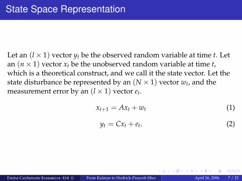
State Space Representation

Let an (l × 1) vector yt be the observed random variable at time t. Letan (n × 1) vector xt be the unobserved random variable at time t,which is a theoretical construct, and we call it the state vector. Let thestate disturbance be represented by an (N × 1) vector wt, and themeasurement error by an (l × 1) vector et.

xt+1 = Axt + wt (1)

yt = Cxt + et. (2)


Noise Processes Assumptions

E(

wte′τ

)= 0 for all t, τ. (3)

E(

wtw′τ

)=

{Q for t = τ0 otherwise,

(4)

E(

ete′τ

)=

{R for t = τ0 otherwise.

(5)


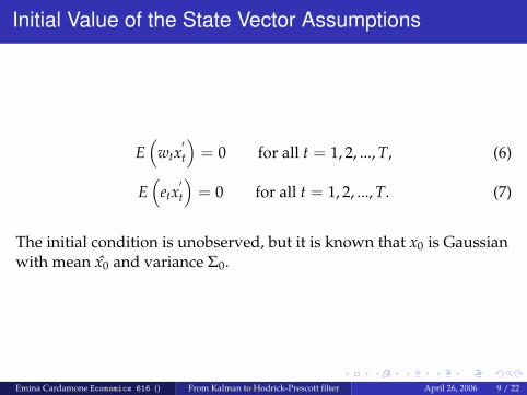
Initial Value of the State Vector Assumptions

E(

wtx′t

)= 0 for all t = 1, 2, ..., T, (6)

E(

etx′t

)= 0 for all t = 1, 2, ..., T. (7)

The initial condition is unobserved, but it is known that x0 is Gaussianwith mean x̂0 and variance Σ0.


Example

Let A = 0.9, C = 1, Σ0 = 40, 000, x0 = 1000, Q = 100, R = 10, 000, andwe observe y1 = 1200.

The results from the time update equations are:x1|0 = Ax0 = 0.9 ∗ 1000 = 900,

Σ1|0 = 0.92 ∗ 40, 000 + 100 = 32, 500.

The results from the measurement update equations are:K1 = Σ1|0C(C2Σ1|0 + R)−1 = 0.7647,

x̂1|1 = x1|0 + K1(y1 − Cx1|0) = 1129,

Σ1|1 = Σ1|0(1 − K1C) + RK21 = 7647.


HP Filter

The HP filter decomposes yt into a time trend or growth component,gt, and a stationary residual or cyclical component ,ct. Then the seriescan be modeled as follows:

yt = gt + ct, (13)

where the unobservable growth component g is

gt = 2gt−1 − gt−2 + εt. (14)


HP Filter State Space Representation

xt =(

gtgt−1

), A =

(2 −11 0

), C =

(1 0

), wt =

(εt0

).


HP Filter

The simple HP filter gives an estimate of the unobserved variable asthe solution to the following minimization problem:

MinT

∑t=1

(yt − gt)2 + λT−1

∑t=2

[(gt+1 − gt)− (gt − gt−1)]2, (15)

with respect to {gt}Tt=1.

The ratio of variances between ct and εt is λ in the HP filter function.We take λ = 1600.


Unit Root Tests

Examine three models:

∆yt = δyt−1 + vt, (16)

such that yt is a random walk,

∆yt = β1 + δyt−1 + vt, (17)

such that yt is a random walk with drift, and

∆yt = β1 + β2t + δyt−1 + vt, (18)

such that yt is a random walk with drift around a stochastic trend.

The hypothesis being tested is whether δ = 0, the time series isnonstationary, against the alternative δ < 0, the time series isstationary.


Unit Root Tests

ADF t statistic Critical Value at 5%5.810 -1.944-0.135 -2.895-1.642 -3.462

Table: Unit Root Test for GDP

Therefore, the data is nonstationary, or in other words, it has a unitroot.


GDP as Sum of Trend Component and CyclicalComponent

1970 1972 1974 1976 1978 1980 1982 1984 1986 1988 19907.92

8.04

8.16

8.28

8.40

8.52LGDPHPSMOOTH

Figure: 1Emina Cardamone Economics 616 () From Kalman to Hodrick-Prescott filter April 26, 2006 17 / 22

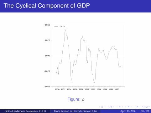
The Cyclical Component of GDP

1970 1972 1974 1976 1978 1980 1982 1984 1986 1988 1990-0.050

-0.025

0.000

0.025

0.050CYCLE

Figure: 2


Conclusion

Present a theoretical overview of the discrete Kalman filter.Test the given theoretical framework empirically.The Hodrick-Prescott (1997) filter was rewritten in a state spaceform, and it was estimated by maximum likelihood method withthe Kalman filter.The nature of the comovements of the cyclical component of theU.S. GDP time series is very different from the comovements ofthe slowly varying trend component.


Extensions

Possible extensions include the following:

Check how different paramter values of λ would change theresults of the estimation.Examine the validity of the model, and the serial correlationproperties of the data.Examine how well the Kalman filter could forecast trends andcycles based on the GDP data that was used in the paper.


References

Hamilton, James, Time Series Analysis, Princeton University Press,Princeton, NJ, 1994.

Bishop, Gary and Welch, Greg, An introduction to the Kalman filter,Department of Computer Science, University of North Carolina atChapel Hill, on the web at http://www.cs.unc.edu/welch.

Moore, John and Anderson, Brian, Optimal filtering, Prentice-Hall, Inc.,Englewood Cliffs, NJ, 1979.


References

Hodrick, Robert J. and Prescott, Edward C., Postwar U.S. BusinessCycles: An Empirical Investigation, Journal of Money, Credit andBanking, Vol. 29, No.1, February 1997.

Kuttner, Kenneth, Estimating potential output as a latent variable,ASA Journal of Business and Economic Statistics, Vol. 12, No. 3, July 1994.

Ljungqvist, Lars and Sargent, Thomas J., Recursive macroeconomictheory, Cambridge, Massachusetts, MIT Press, 2004.


From Kalman to Hodrick-Prescott ﬁlter - ubalt.edu Kalman to Hodrick-Prescott ﬁlter Theory and...

Documents

Transcript of From Kalman to Hodrick-Prescott ﬁlter - ubalt.edu Kalman to Hodrick-Prescott ﬁlter Theory and...