From forward modelling of MT phases over 90 towards 2D...

From forward modelling of MT phases over 90◦ towards

2D anisotropic inversion

X. Chen1,2, U. Weckmann1, K. Tietze1,3

1Helmholtz Centre Potsdam - German Research Center for Geosciences,Germany

2University of Potsdam, Institute of Geosciences, Germany

3Free University of Berlin, Institute of Geological Sciences, Germany

[email protected], [email protected], [email protected]

Abstract

Within the framework of the German - South African geo-scientific research initiative Ink-

aba yeAfrica several magnetotelluric (MT) field experiments were conducted along the Agulhas-

Karoo Transect in South Africa. This transect crosses several continental collision zones between

the Cape Fold Belt, the Namaqua Natal Mobile Belt and Kaapvaal Craton. Along the profile

we can identify areas (> 10km) with phases over 90◦. This phenomenon usually occurs in pres-

ence of electrical anisotropy. Due to the dense site spacing we are able to observe this behaviour

consistently at several sites.

In this presentation we focus on the profile section between Prince Albert and Mosselbay. With

isotropic 2D inversion we are able to explain most features in the MT data but not the abnormal

phase behavior. With several anisotropic forward modelling studies we have tested the influence

of anisotropy parameters on the MT responses. In a first step we use simple 2D models with

embedded zones of electrical anisotropy to get a basic understanding of anisotropic responses. In

a second step isotropic 2D inversion results serve as background models in which we included

anisotropic zones, e.g. to fit the abnormal phase curves. These resolution tests are necessary and

important for the future development of a 2D inversion with spatially constraint anisotropy.

1 IntroductionFor a 2D geoelectric model with a finite system of homogeneous, but generaly anisotropic blocks the

electrical conductivity is a tensor instead of a scalar quantity. It is symmetric and positive-definite.

Due to its symmetry the conductivity tensor σ within each layer of model can be diagonalized and ex-

pressed by three principal conductivities σ1, σ2, σ3 and a rotation matrix, which can be decomposed

into three elementary Euler’s rotations αS, αD, αL respectively.

σ =

⎛⎝ σxx σxy σxz

σyx σyy σyzσzx σzy σzz

⎞⎠

= Rz(−αS)Rx(−αD)Rz(−αL)

⎛⎝ σ1 0 0

0 σ2 0

0 0 σ3

⎞⎠Rz(αL)Rx(αD)Rz(αS)

where Rx and Rz are elementary rotation matrices around the coordinate axis x and z, respectively.The

angles αS, αD, αL are typically called anisotropy strike, dip and slant, respectively.

In this work we investigate the feasibility of use of 2D forward anisotropy modelling to simulate

phases over 90◦ which we observed in field data from the MT survey in South Africa. Using the 2D

anisotropy forward modelling algorithm of Pek and Verner (1997) we vary the model parameters in23. Schmucker-Weidelt-Kolloquium für Elektromagnetische Tiefenforschung,

Heimvolkshochschule am Seddiner See, 28 September - 2 Oktober 2009 88

order to gain a basic understanding of the MT transfer function in presence of anisotropy. First we

will give a brief introduction of the survey area and then we will show the results of 2D isotropic

inversion and 2D anisotropic forward modelling.

2 Survey areaWithin the framework of the German - South African geo-scientific research initiative Inkaba yeAfrica

four magnetotelluric (MT) field experiments were conducted along the Agulhas-Karoo Transect in

South Africa (Weckmann et al., 2007, Stankiewicz et al., 2008). These transects cross several con-

tinental collision zones and their respective units, such as the Cape Fold Belt, the Namaqua Natal

Mobile Belt and the Kaapvaal Craton. The MT profile on which we focus in this paper is located in

AgulhasPlateau

CFB

Agulhas-Falkland Fracture Zone

Mo

zam

biq

ue

Rid

ge

MT

NVR

WRR

SCCB

BMA

Offshore seismics

KaapvaalCraton

Karoo

TranskeiBasin

MT2 profile

NNMBSCCB

Figure 1: Left: Map of the Agulhas-Karoo Geoscience Transect with MT Profiles (red lines) across

Cape Fold Belt , the Namaqua Natal Mobile Belt and the Kaapvaal Craton. Right: The profile MT2

contains 46 broad band MT sites and 8 broad band / long period MT sites. It extends 120 km from

Prince Albert in the North to Mosselbay in the South and covers the entire Cape Fold Belt.

the Cape Fold Belt. In total, 54 MT sites were deployed along this 120 km long profile MT 2 (Fig. 1).

It extends from Prince Albert in the North to Mosselbay in the South and covers the entire Cape Fold

Belt (CFB), its inliers, the Oudtshoorn and the Kaaimans Basins, the Swartberg and the Outeniequa

Mountain ranges and several major thrusts and faults.

3 Data and isotropic 2D inversionAlong the profile MT2 we acquired 5-component MT data at all stations in a period range from

0.001s to 1000s using GPS synchronized S.P.A.M. MkIII (Ritter et al., 1998) and CASTLE broadband

instrument. Metronix MFS06/06 induction coil magnetometer and non-polarizable Ag/AgCl telluric

electrodes were used to record natural magnetic and electric field variations. The data were processed

with the EMERALD software package (Ritter et al., 1998) using both robust single site and remote

reference techniques. At some sites, for which a suitable reference site was not available and the

data were affected by cultural noise (extensive farming), we applied the frequency domain selection

scheme after Weckmann et al. (2005) to improve data quality.

23. Schmucker-Weidelt-Kolloquium für Elektromagnetische Tiefenforschung, Heimvolkshochschule am Seddiner See, 28 September - 2 Oktober 2009

89

Figure 2: Pseudo-sections of TE and TM mode apparent resistivity and phase (x direction pointing

west).We can observe phase values over 90 degrees in the middle of the profile in both TE and TM

component (marked with black ellipses in the upper panel). Two exemplary sites (site 121 and site

116) are displayed as apparent resistivity, phase and induction arrows (Wiese convention) over period.

The red arrows in the pseudo-sections show the location of the selected sites. We can identify that the

phases, (especially in the TE component) leave the first quadrant at a minimum period of 10 s, but

typically at longer periods of 100-1000 s.


90

After data processing, we applied different strike and dimensionality analyses, e.g. the ellipticity

analysis after Becken & Burkhardt (2004), obtaining an electromagnetic strike direction of −90◦, i.e.

East-West direction. This is in general compatible with the tectonic grain of the CFB. Furthermore,

most of the data seem to be compatible with a 2D interpretation approach. However, in a limited area

we observe impedance phases exceeding 90 degrees at long periods. They typically appear in both,

TE and TM mode, and persit in either component even if we rotate the coordinate system (Fig. 2).

Figure 3: TE and TM mode data used for isotropic 2D inversion. Prior to inversion they were rotated

into a common coordinate system according to the geoelectric strike direction of ≈ 90◦ (obtained by

strike and phase tensor analysis). Data with phases over 90◦ are discarded from the data base.

For an isotropic 2D inversion approach we use RLM2D (Rodi & Mackie, 2001, implemented in

the WinGlink software package). Before starting a 2D inversion we have to make sure that large phase

values over 90◦ are excluded as they cannot be fitted by a 2D inversion approach. Figure 3 shows

the data which were finally used for 2D inversion. Figure 4 displays our preferred 2D conductivity

image of the upper 35 km together with a section of the geological map after Halbich et al. (1993).

The inversion was started from a homogeneous half-space of 100Ωm with τ = 10 using TE and

TM component, with intermediate inclusion of the vertical magnetic transfer function. Within the

framework of this work, we refrain from interpreting conductivity anomalies in a geological context,

but focus on the area where phases over 90◦ occur. One of the most prominent conductivity anomalies

is a triangular shaped, highly conductive structure in the middle of the profile. In this area we also

observe phases leaving the quadrant. This conductivity anomaly is required by the data which is

compatible with a 2D interpretation approach; however, we believe that the phases over 90◦ are caused

by some electrically anisotropic structures in this area (in Fig. 4 between black dashed lines). We

should also note that the deep part of this area only possesses a very limited resolution (in Fig. 4

marked with semitransparent mask) because most of the data which relates to this part are excluded

in order to satisfy the 2D isotropic procedure (see Fig. 3). Similar phase behaviour was explained

with crustal anisotropy by Weckmann et al. (2003) and Heise & Pous (2003), where data within old

continental collision zones in Namibia and on the Iberian Peninsula, respectively. In both cases the

data could be fit by using a shallow and a deeper electrically anisotropic zone with different anisotropy

strike.

4 Anisotropic forward modellingIsotropic 2D inversion is adequate to explain the data in most parts along the profile but it is very

unsatisfactory not being able to include phases greater than 90 degrees and thus neglect a substantial

amount of data. In order to develop a 2D inversion with spatially constraint anisotropy, resolution

tests and synthetic modelling studies are necessary. In a first step towards the constraint anisotropic23. Schmucker-Weidelt-Kolloquium für Elektromagnetische Tiefenforschung,

Heimvolkshochschule am Seddiner See, 28 September - 2 Oktober 2009 91

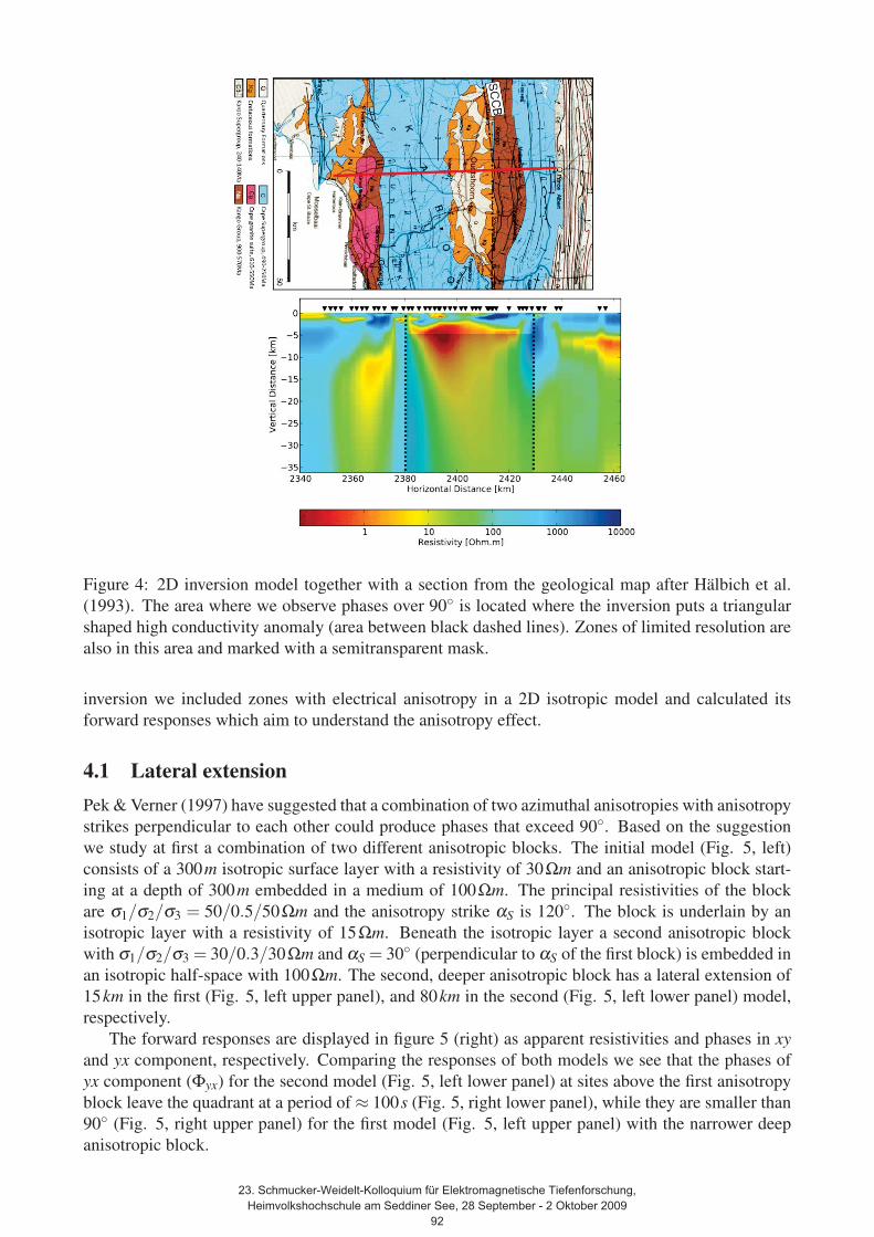
Figure 4: 2D inversion model together with a section from the geological map after Halbich et al.

(1993). The area where we observe phases over 90◦ is located where the inversion puts a triangular

shaped high conductivity anomaly (area between black dashed lines). Zones of limited resolution are

also in this area and marked with a semitransparent mask.

inversion we included zones with electrical anisotropy in a 2D isotropic model and calculated its

forward responses which aim to understand the anisotropy effect.

4.1 Lateral extensionPek & Verner (1997) have suggested that a combination of two azimuthal anisotropies with anisotropy

strikes perpendicular to each other could produce phases that exceed 90◦. Based on the suggestion

we study at first a combination of two different anisotropic blocks. The initial model (Fig. 5, left)

consists of a 300m isotropic surface layer with a resistivity of 30Ωm and an anisotropic block start-

ing at a depth of 300m embedded in a medium of 100Ωm. The principal resistivities of the block

are σ1/σ2/σ3 = 50/0.5/50Ωm and the anisotropy strike αS is 120◦. The block is underlain by an

isotropic layer with a resistivity of 15Ωm. Beneath the isotropic layer a second anisotropic block

with σ1/σ2/σ3 = 30/0.3/30Ωm and αS = 30◦ (perpendicular to αS of the first block) is embedded in

an isotropic half-space with 100Ωm. The second, deeper anisotropic block has a lateral extension of

15km in the first (Fig. 5, left upper panel), and 80km in the second (Fig. 5, left lower panel) model,

respectively.

The forward responses are displayed in figure 5 (right) as apparent resistivities and phases in xyand yx component, respectively. Comparing the responses of both models we see that the phases of

yx component (Φyx) for the second model (Fig. 5, left lower panel) at sites above the first anisotropy

block leave the quadrant at a period of ≈ 100s (Fig. 5, right lower panel), while they are smaller than

90◦ (Fig. 5, right upper panel) for the first model (Fig. 5, left upper panel) with the narrower deep

anisotropic block.


92

Figure 5: Models (left) and their forward responses (right). The models differ only in lateral extension

of anisotropy block. The lateral extension of the second block is about 15km in the first model (left

upper panel) and 80km (left lower panel) in the second model. The major difference in the responses

appears in the yx component. Phases over 90◦ occur if the lateral extension of the deeper anisotropy

block is greater than it of the shallower anisotropy block.

4.2 DepthIn a second step, we used the same anisotropy parameters as described above. The initial model

consists of a 300m isotropic surface layer and a isotropic half-space with resisitivity of 100Ωm. Two

anisotropy blocks are embedded in the half-space. The first block started at depth of 300m and shaped

as a trapezoid. In this attempt we vary the depth of the second block. In the first model (Fig. 6, left

upper panel) the second block started at a depth of 1.8km and in the second model (Fig. 6, left lower

panel) started at a depth of 6.8km.

In the forward responses (Fig. 6, right) we see that the phases Φyx for the second model become

larger than 90◦ at periods > 10s at sites above the first block, while they for the first model are

all smaller than 90◦. In this attempt the second anisotropy block has always sufficiently greater

lateral extension than the first anisotropy block, but we only see the phase anomalies by model with

anisotropy block in adequate depth. Besides the lateral extension of the anisotropy block, also the

depth is one of those key conditions under which phase anomalies appear.

4.3 Rotation angleIn a third test we use a similar model as described above for step two. The model contains a 300misotropic surface layer and an isotropic half-space with resisitivity of 100Ωm. Two anisotropic blocks

are embedded in the half-space. The first block starts directly beneath the surface layer and the

second block in a depth of 6km. They have the principal resistivities σ1/σ2/σ3 = 50/0.5/50Ωm and

σ1/σ2/σ3 = 30/0.3/30Ωm, respectively. In this attempt we vary the anisotropy strike angle αS1 and

αS2 for both blocks.

The forward response for the model with αS1 = αS2 = 0◦ is displayed in the right upper panel

of figure 7. The phases of the yx component approach 90◦ for long periods. For αS1 = 60◦ and

αS2 = 120◦ (Fig. 7, left lower panel) the yx component phases become larger than 90◦ for periods

> 10s, while they stay below 90◦ for αS1 = 90◦ and αS2 = 120◦ (Fig. 7, right lower panel). Comparing

the three examples, we see that model with different combination of strike angle in both shallow and


93

Figure 6: Models (left) and their forward responses (right). The models differ by depth of the second

anisotropy block. In the first model (left upper panel) the second block starts in a depth of 1.8kmand in the second model (left lower panel) the block starts in a depth of 6.8km. The phases of yxcomponent for the model with the deeper anisotropic block become larger than 90◦ at periods > 10sat sites above the first block. For the model with the shallower block all phases are smaller than 90◦.

αS1 and αS2 αS1 = 0◦ and αS2 = 0◦

αS1 = 60◦ and αS2 = 120◦ αS1 = 90◦ and αS2 = 120◦

Figure 7: Model (left upper panel) and its forward responses with different anisotropy strike angles.

The model contains the same surface layer, background medium and resistivities for both anisotropic

blocks as the models in fig. 6. We vary the strike angles αS1 and αS2 for the shallow and the deep

block (left upper panel). The forward responses are displayed as apparent resistivities and phases in

xy and yx component.


94

deep blocks produce forward responses with pronounced difference. This can be observed not only in

yx component (ρa(yx) and Φyx ) but also in xy component (ρa(xy) and Φxy ). A possible explanation is

that a change of strike angle forces the current flow to change its preferred direction from the shallow

to the deep block. According to this fact we may conclude that the anisotropy strike angle influences

forward responses significantly and phase greater than 90◦ will appear if the strike angle of both

blocks differ by an adequate amount.

5 ConclusionsPhases greater than 90◦ can only be modelled by a combination of a deep and a shallow anisotropic

block. We varied several model parameters to study the changes in forward responses. For our models

we can conclude that phases out of the first quadrant occur when: (i) the anisotropy ratio (σmax/σmin)

is high (for both blocks); (ii) the deep anisotropic block has a much larger lateral extension than the

shallow block; (iii) the deep anisotropic block is located in greater depth; (iv) the angles of anisotropy

of both blocks differ by a considerable amount. In our models the difference should be at least 45◦ so

that the preferred direction of current flow changes significantly from the shallow to the deep block.

ReferencesBecken, M., & Burkhardt, H. (2004). An ellipticity criterion in magnetotelluric tensor analysis.

Geophys. J. Int., 159, 69–82.

Eisel, M., & Haak, V. (1999). Macro-anisotropy os the electrical conductivity of the crust: a magneto-

telluric study from the German continental Deep Drilling site (KTB). Geophys. J. Int., 136, 109–

122.

Halbich, I. (1993). Cape Fold Belt – Agulhas Bank Transect across Gondwana suture, southern

Africa. Geosci. Transect, 9, 18 pp. AGU, Washington, D. C.

Heise, W., & Pous, J. (2003). Anomalous phases exceeding 90◦ in magnetotellurics: anisotropic

model studies and a field example. Geophys. J. Int., 155, 308–318.

Kellett, R. L., Mareschal, M., & Kurtz, R. D. (1992). A model of lower crustal electrical anisotropy

for the Pontiac Subprovince of the Canadian Shield. Geophys. J. Int., 111, 141–150.

Mareschal, M., Kellett, R. L., Kurtz, R. D., Ludden, J. N., Ji, S., & Bailey, R. C. (1995). Archaean

cratonic roots, mantle shear zones and deep electrical anisotropy. Nature, 375, 134–137.

O’Brien, D. P., & Morrison, H. F. (1967). Electromagnetic fields in an N-layer anisotropic half space.

Geophysics, 32, 668–677.

Pek, J., & Verner, T. (1997). Finite-difference modelling of magneto-telluric fields in two-dimensional

anisotropic media. Geophys. J. Int., 128, 505–521.

Reddy, I. K., & Rankin, D. (1975). Magnetotelluric response of lateerally inhomogeneous and

anisotropic media. Geophysics, 40, 1035–1045.

Ritter, O., Junge, A., & Dawes, G. J. K. (1998). New equipment and processing for magnetotelluric

remote reference observations. Geophys. J. Int., 132, 535–548.

Rodi, W., & Mackie, R. L. (2001). Nonlinear conjugate gradients algorithm for 2-d magnetotelluric

inversion. Geophysics, 66, 174–187.


95

Stankiewicz, J., Ryberg, T., Schulzw, A., Lindeque, A., Weber, M., & de Wit, M. (2007). Initial

results from wide-angle seismic refraction lines in the southern Cape. South African Journal ofGeology, 110, 407–418.

Weckmann, U., Jung, A., Branch, T., & Ritter, O. (2007). Comparison of electrical conductivity

structures and 2D magnetic modelling along two profiles crossing the Beattie Magnetic Anomaly,

South Africa. South African Journal of Geology, 110, 449–464.

Weckmann, U., Magunia, A., & Ritter, O. (2005). Effective noise separation for magnetic single site

data processing using a frequency domain selection scheme. Geophys. J. Int., 161, 635–652.

Weckmann, U., Ritter, O., & Haak, V. (2003). A magnetotelluric study of the damara belt in namibia

– 2. MT phases over 90◦ reveal the internal structure of the Waterberg Fault/Omaruru Lineament.

Phys. Earth Planet. Inter., 138(2), 91–112.


96

From forward modelling of MT phases over 90 towards 2D...

Documents

Transcript of From forward modelling of MT phases over 90 towards 2D...