
'Deixis and Pragmatics' for Handbook of Pragmatics Stephen C ...

Dines Bjørner∗
From Domains to RequirementsThe Triptych Approach to Software Engineering
August 30, 2009: 13:10
To be submitted, Summer 2009, to Springer
Berlin Heidelberg NewYorkHongKong LondonMilan Paris Tokyo
∗Fredsvej 11, DK-2840 Holte, Danmark, E–Mail: [email protected], URL: www.imm.dtu.dk/˜db

VI
s1
c© 2009 Dines Bjørner

Dedication
My parents:
Else Margrethe Sigrid Bjørner (Christensen) 1905–1993Ivar Hainau (Christensen) 1907–1971
— for a classical childhood and youth.


Part I
Opening

Preface
acm-abs
This Textbook is Different ! s2
This textbook is different in a number of ways:
1. The Triptych Dogma : The dogma “says”:
• Before software can be designed one must understand the requirements.• Before requirements can be prescribed one must understand the domain.
This dogma carries the two main parts of the book:
• Part IV: Domains and• Part V: Requirements.
No other ‘Software Engineering’ textbook (other than [19] of the approximately 2400page [17–19]) propagates this dogma.
2. Domain Engineering : s3
This is a new phase of software development. It is thoroughly treated in Chap. 7. It is explainedand motivated in Chaps. 2–3.
No other ‘Software Engineering’ textbook (other than [19]) covers ‘Domain Engineer-ing’ — and the present volume covers that topic in a novel (read: “improved”) way.
3. Derivation of Requirements from Domain Models : s4
Requirements development is here presented in a way which differs fundamentally and signif-icantly from how it has been presented by past textbooks on ‘Software Requirements Engi-neering’. This novel and simpler approach, as based on careful domain descriptions, both innarrative and in formal form is thoroughly treated in Chap. 8.
No other ‘Software Engineering’ textbook (other than [19]) covers Requirements Engi-neering in this novel and logical way and the current treatment significantly improvesthat of [19].
4. Proper Conceptualisation (Part III): s5
Software development is a highly intellectual process. Among the constituent sets of theories,principles and techniques of software development are those of ‘Abstraction & Modelling’,‘Semiotics’ and ‘Specification Ontology’. These are treated in separate chapters of this book.
No other ‘Software Engineering’ textbook (other than [17–19]) covers these three con-cepts, ‘Abstraction & Modelling’, ‘Semiotics’ and ‘Specification Ontology’, in this sim-plified way.
We shall very briefly explain these three concepts. s6
4.1 Abstraction & Modelling Chapter 4:Abstraction relates to conquering complexity of description through the judicious use ofabstraction, where abstraction, briefly, is the act and result of omitting consideration of(what would then be called) details while, instead, focusing on (what would therefore becalled) important aspects.

XII
s7
Modelling relates to choosing between (i) property- and model-oriented specification; (ii)a suitable balance between analogic, analytic and iconic modelling; (iii) descriptive andprescriptive modelling as for domain modelling, respectively requirements modelling; and(iv) extensional versus intentional models.Modelling also has to decide “for which purposes” a model shall serve: to gain understanding,to get inspiration and to inspire, to present, educate and train, to assert and predict and toimplement requirements derived from domain models.
4.2 Semiotics Chapter 5: s8
Semiotics deal with the form, i.e., the syntax, in which we express concepts; the meaning,i.e., the semantics, of what is being expressed; and the reason, i.e., the pragmatics, of whywe express something and the chosen form of expression.Since all we really ever do when expressing domains, requirements and software is toproduce textual documents it is of utmost importance that we command these three facetsof semiotics.
4.3 Specification Ontology 1 Chapter 6: s9
How do we present descriptions ? The technical means of expressing the phenomena andconcepts of domains form a meta-ontology. And the description itself is an ontology ofthe domain. In Chap. 6 we advance three “faces” of ontological nature: (i) the simpleentity, operation, event and behaviour approach to description; (ii) the mereology of simpleentities; and (iii) the laws of description !
Our treatment of ‘Abstraction & Modelling’, ‘Semiotics’ and ‘Specification Ontology’,above are quite novel and constitute, in our opinion, quite a significant improvementof [19].
5. Examples : s10
The book carries more that 140 substantial both informal and formal examples. Almost halfare several pages long.
No other ‘Software Engineering’ textbook (not even [17–19]) carries so many informal-&formal examples, examples that are substantial — and the present volume ties themany examples more strongly together.
6. Projects : s11
In Appendix D there is a list of annotated course project proposals. A course — based onthis book — is proposed to consist of both ‘formal’ class lectures — covering this book —and ‘informal’ tutoring sessions —advising students on how to proceed using the book in engi-neering both a domain description and a requirements prescription for one of the projects listed inAppendix D. That appendix will give some hints, to both lecturers (course project tutors) andstudents. Hints to lecturers on how to use this book in the ‘formal’ class lectures is given in as12
separate booklet that is (i.e., will be) available on the Internet.We cannot overemphasise the pedagogical and didactical need to both give the ‘formal’ classlectures and the course project ‘informal’ tutoring sessions:• “learn by doing”• “but on a science-based foundation”.
Chapter-by-Chapter Overviews13
(Chapter 1) We start by providing a background for this study.s14
1Ontology is the philosophical study of the nature of being, existence or reality in general, as well asof the basic categories of being and their relations. Traditionally listed as a part of the major branch ofphilosophy known as metaphysics, ontology deals with questions concerning what entities exist or can besaid to exist, and how such entities can be grouped, related within a hierarchy, and subdivided accordingto similarities and differences [Wikipedia].

XIII
(Chapter 2) We introduce the concepts of domains, that is, potential or actual application domainsfor software. s15
(Chapter 3) We then motivate the study of domains where such studies aim at creating both preciseinformal and formal descriptions of domains – (and) where formal descriptions are limited to what we cantoday mathematically formalise. s16
(Chapter 4) Abstraction and modelling are keywords in specifications and we shall therefore verybriefly summarise a few key concepts – including property- and model-oriented abstractions. We shallalso, likewise very briefly, overview a tool for formal abstraction: the main specification language. RSL, ofthis book and its use in achieving abstractions. s17
(Chapter 5) We take a very brief look at issues of semiotics: pragmatics, semantics and syntax. Theprime goal of software engineering work is description, prescription and specification, that is: producingdocuments, that is, informal and formal texts. Texts have syntax — what we write has meaning (i.e.,semantics), and the reason we wrote it down is motivated, i.e., is pragmatics. s18
(Chapter 6) What is it that we are describing (as for domains), prescribing (as for requirements)and specifying (as for software designs)? We shall suggest that the descriptions (etc.) focus on entitiesand behaviours, functions and events – and shall therefore briefly summarise these concepts (and likewisebriefly exemplify their abstract modelling) before deploying this “specification ontology” in domain andin requirements engineering. s19
(Chapter 7) Domain engineering is then outlined in terms of its many stages: [i] information documentcreation, [ii] identification of domain stake-holders, [iii] business process rough sketching, [iv] domain ac-quisition, [v] domain analysis and concept formation, [vi] domain terminologisation, [vii] domain modelling– the major stage – [viii] domain model verification (checking, testing), [ix] domain description validation,and [x] domain theory creation. Emphasis is put on business process description (Sect. 7.2) and on the s20
six sub-stages of domain modelling: (a) intrinsics, (b) support technologies, (c) management and organ-isation, (d) rules and regulations, (e) scripts and (f) human behaviour (Sects. 7.3–7.8). A final section,Sect. 7.9 summarises the opening and closing stages of domain engineering: stakeholder identification andliaison, acquisition, business processes, terminoligisation, respectively verification, model checking, testing,validation and domain theory issues. s21
(Chapter 8) It is finally outlined, in some detail, how major parts of requirements can be system-atically “derived” from domain descriptions: in three major sub-stages: [A] domain requirements, [B]interface requirements and [C] machine requirements – where our contribution is solely placed in sub-stages [A–B]. In this part it is briefly argued why current requirements engineering appears to be based s22
on a flawed foundation. Emphasis is put on the pivotal steps of domain requirements in which (a) businessprocesses are re-engineering (Sect. 8.5); (b) domain requirements are projected, instantiated, made moredeterministic, extended and fitted (Sect. 8.6); (c) interface requirements are “created” while consideringthe simple entities, functions, events and behaviours shared that are (to be) shared between the domainand the machine (Sect. 8.8); and (d) machine requirements are laboriously enumerated and instantiated(Sect. 8.9). A final section, Sect. 8.10 summarises the opening and closing stages of requirements engineer- s23
ing: stakeholder identification and liaison, acquisition, business process re-engineering, terminoligisation,respectively verification, model checking, testing, validation, satisfiability & feasibility and requirementstheory issues.
A Lecture Schedule Proposal
Each of the lectures, Lectures 1–18, listed below, is thought of as a double lecture session of (two)50 minute lectures separated by a 10 minute break.
Lectures marked (⊖) can be omitted entirely.In this way the listed 18 lectures can be “cut” to 14.
1. Lecture 1:
• Opening XII–XIII• Background 3–4
2. Lecture 2:• What are Domains ? 5–18• Motivation for Domain Engineering 19–
20
3. Lecture 3: Abstraction & Modelling – I
• Abstraction 23–27
4. Lecture 4: Abstraction & Modelling – II
• Abstraction 27–31
• Modelling 31–35
5. Lecture 5: Semiotics ⊖

XIV
• Syntax 37–46• Semantics & Pragmatics 46–53
6. Lecture 6: A Specification Ontology – I
• Simple Entities 55–63• Behaviours 63–66
7. Lecture 7: A Specification Ontology – II
• Functions 66–69• Events 69–73
8. Lecture 8: Domain Engineering – I
• Opening Stages 77–84• Intrinsics 84–88
9. Lecture 9: Domain Engineering – II
• Supp.Techns. 88–93• Mgt. & Org. 93–96
10. Lecture 10: Domain Engineering – III
• Rules & Regs. 96–98
• Scripts 98–123
11. Lecture 11: Domain Engineering – IV
• Human Behaviour 123–128• Closing Stages 128–129
12. Lecture 12: Requirements Engineering – I
• Opening Stages and Acquisition 133–134• Business Processes 134–141
13. Lecture 13: Requirements Engineering – II
• Domain Requirements 141–153
14. Lecture 14: Requirements Engineering – III
• Interface Requirements 153–164
15. Lecture 15: Requirements Engineering – IV
• Machine Requirements 165–173• Closing Stages 173–174• Closing 177–177
Appendix C (Pages 223–228). provides a lecturers’ guide to using this textbook.
Course Project Tutoring
In addition to the lectures it is strongly suggested that each day, for example, a morning doublelecture is given, there is also an afternoon two hour project tutoring session. More about this inAppendix. D (Pages 229–234).

Contents
Dedication . . . . . . . . . . . . . . . . . . . . . . . . . . . . . . . . . . . . . . . . . . . . . . . . . . . . . . . . . . . . . . . . . . . . . . . . . . . . . . VII
Part I Opening
Preface . . . . . . . . . . . . . . . . . . . . . . . . . . . . . . . . . . . . . . . . . . . . . . . . . . . . . . . . . . . . . . . . . . . . . . . . . . . . . . . . . XIThis Textbook is Different ! . . . . . . . . . . . . . . . . . . . . . . . . . . . . . . . . . . . . . . . . . . . . . . . . . . . . . . . . . . . . XIChapter-by-Chapter Overview . . . . . . . . . . . . . . . . . . . . . . . . . . . . . . . . . . . . . . . . . . . . . . . . . . . . . . . . . . XIIA Lecture Schedule Proposal . . . . . . . . . . . . . . . . . . . . . . . . . . . . . . . . . . . . . . . . . . . . . . . . . . . . . . . . . . . XIII
Course Project Tutoring . . . . . . . . . . . . . . . . . . . . . . . . . . . . . . . . . . . . . . . . . . . . . . . . . . . . . . . . . XIV
Part II Introduction
1 Background . . . . . . . . . . . . . . . . . . . . . . . . . . . . . . . . . . . . . . . . . . . . . . . . . . . . . . . . . . . . . . . . . . . . . . . . . 3
2 What are Domains? . . . . . . . . . . . . . . . . . . . . . . . . . . . . . . . . . . . . . . . . . . . . . . . . . . . . . . . . . . . . . . . . . 52.1 Delineation . . . . . . . . . . . . . . . . . . . . . . . . . . . . . . . . . . . . . . . . . . . . . . . . . . . . . . . . . . . . . . . . . . . 5
Definition 1: Domain . . . . . . . . . . . . . . . . . . . . . . . . . . . . . . . . . . . . . . . . . . 5Definition 2: Domain Description . . . . . . . . . . . . . . . . . . . . . . . . . . . . . . . 5
2.1.1 Elements, Aims and Objectives of Domain Science(I) . . . . . . . . . . . . . . . . . . . . . . 5Definition 3: Phenomenon . . . . . . . . . . . . . . . . . . . . . . . . . . . . . . . . . . . . . 5Definition 4: Concept . . . . . . . . . . . . . . . . . . . . . . . . . . . . . . . . . . . . . . . . . 5
2.1.2 Physics versus Domain Science . . . . . . . . . . . . . . . . . . . . . . . . . . . . . . . . . . . . . . . . . 6General . . . . . . . . . . . . . . . . . . . . . . . . . . . . . . . . . . . . . . . . . . . . . . . . . . . . . . . . . . . . . . 6Spatial Attributes of Phenomena and Concepts . . . . . . . . . . . . . . . . . . . . . . . . . . . 7Simple Entities versus Attributes . . . . . . . . . . . . . . . . . . . . . . . . . . . . . . . . . . . . . . . . 7
2.1.3 Constituent Sciences of Domain Science . . . . . . . . . . . . . . . . . . . . . . . . . . . . . . . . . 7Knowledge Engineering . . . . . . . . . . . . . . . . . . . . . . . . . . . . . . . . . . . . . . . . . . . . . . . . 7Computer Science . . . . . . . . . . . . . . . . . . . . . . . . . . . . . . . . . . . . . . . . . . . . . . . . . . . . . 7
Definition 5: Computer Science . . . . . . . . . . . . . . . . . . . . . . . . . . . . . . . . 7Computing Science . . . . . . . . . . . . . . . . . . . . . . . . . . . . . . . . . . . . . . . . . . . . . . . . . . . . 7
Definition 6: Computing Science . . . . . . . . . . . . . . . . . . . . . . . . . . . . . . . 72.1.4 Elements, Aims and Objectives of Domain Science (II) . . . . . . . . . . . . . . . . . . . . 7
2.2 Informal Examples . . . . . . . . . . . . . . . . . . . . . . . . . . . . . . . . . . . . . . . . . . . . . . . . . . . . . . . . . . . . . 8Example 1: Air Traffic (I) . . . . . . . . . . . . . . . . . . . . . . . . . . . . . . . . . . . . . 8Example 2: Banking . . . . . . . . . . . . . . . . . . . . . . . . . . . . . . . . . . . . . . . . . . 8Example 3: Container Line Industry . . . . . . . . . . . . . . . . . . . . . . . . . . . . 8Example 4: Health Care . . . . . . . . . . . . . . . . . . . . . . . . . . . . . . . . . . . . . . . 8Example 5: “The Market” . . . . . . . . . . . . . . . . . . . . . . . . . . . . . . . . . . . . . 8Example 6: Oil Industry . . . . . . . . . . . . . . . . . . . . . . . . . . . . . . . . . . . . . . . 8Example 7: Public Government . . . . . . . . . . . . . . . . . . . . . . . . . . . . . . . . 8Example 8: Railways . . . . . . . . . . . . . . . . . . . . . . . . . . . . . . . . . . . . . . . . . . 9

XVI Contents
Example 9: Road System . . . . . . . . . . . . . . . . . . . . . . . . . . . . . . . . . . . . . . 92.3 An Initial Domain Description Example . . . . . . . . . . . . . . . . . . . . . . . . . . . . . . . . . . . . . . . . . . 9
Example 10: Transport Net (I) . . . . . . . . . . . . . . . . . . . . . . . . . . . . . . . . . 92.4 Preliminary Summary . . . . . . . . . . . . . . . . . . . . . . . . . . . . . . . . . . . . . . . . . . . . . . . . . . . . . . . . . . 172.5 Structure of Book . . . . . . . . . . . . . . . . . . . . . . . . . . . . . . . . . . . . . . . . . . . . . . . . . . . . . . . . . . . . . 172.6 Exercises . . . . . . . . . . . . . . . . . . . . . . . . . . . . . . . . . . . . . . . . . . . . . . . . . . . . . . . . . . . . . . . . . . . . . 18
3 Motivation for Domain Descriptions . . . . . . . . . . . . . . . . . . . . . . . . . . . . . . . . . . . . . . . . . . . . . . . . . . . 193.1 Domain Descriptions of Infrastructure Components . . . . . . . . . . . . . . . . . . . . . . . . . . . . . . . 193.2 Domain Descriptions for Software Development . . . . . . . . . . . . . . . . . . . . . . . . . . . . . . . . . . . 19
Dogma: The D,S |= R Dogma . . . . . . . . . . . . . . . . . . . . . . . . . . . . . . . . . 203.3 Discussion . . . . . . . . . . . . . . . . . . . . . . . . . . . . . . . . . . . . . . . . . . . . . . . . . . . . . . . . . . . . . . . . . . . . 20
Part III Proper Conceptualisation
4 Abstraction & Modelling . . . . . . . . . . . . . . . . . . . . . . . . . . . . . . . . . . . . . . . . . . . . . . . . . . . . . . . . . . . . . 234.1 Abstraction . . . . . . . . . . . . . . . . . . . . . . . . . . . . . . . . . . . . . . . . . . . . . . . . . . . . . . . . . . . . . . . . . . . 23
4.1.1 From Phenomena to Concepts . . . . . . . . . . . . . . . . . . . . . . . . . . . . . . . . . . . . . . . . . . 234.1.2 From Narratives to Formalisations . . . . . . . . . . . . . . . . . . . . . . . . . . . . . . . . . . . . . . . 234.1.3 Examples of Abstraction . . . . . . . . . . . . . . . . . . . . . . . . . . . . . . . . . . . . . . . . . . . . . . . 23
Example 11: Model-oriented Directory . . . . . . . . . . . . . . . . . . . . . . . . . . 24Example 12: Networked Social Structures . . . . . . . . . . . . . . . . . . . . . . . 24Example 13: Railway Nets . . . . . . . . . . . . . . . . . . . . . . . . . . . . . . . . . . . . . 24Example 14: A Telephone Exchange . . . . . . . . . . . . . . . . . . . . . . . . . . . . 27Formalisation of Property-oriented State . . . . . . . . . . . . . . . . . . . . . . . . . . 28Operation Signatures . . . . . . . . . . . . . . . . . . . . . . . . . . . . . . . . . . . . . . . . . . 29Model-oriented State . . . . . . . . . . . . . . . . . . . . . . . . . . . . . . . . . . . . . . . . . . 29Efficient States . . . . . . . . . . . . . . . . . . . . . . . . . . . . . . . . . . . . . . . . . . . . . . . 30Formalisation of Action Types . . . . . . . . . . . . . . . . . . . . . . . . . . . . . . . . . . 30Pre/Post and Direct Operation Definitions . . . . . . . . . . . . . . . . . . . . . . . . 30Multi-party Call . . . . . . . . . . . . . . . . . . . . . . . . . . . . . . . . . . . . . . . . . . . . . . 30Call Termination . . . . . . . . . . . . . . . . . . . . . . . . . . . . . . . . . . . . . . . . . . . . . . 30Subscriber Busy . . . . . . . . . . . . . . . . . . . . . . . . . . . . . . . . . . . . . . . . . . . . . . 31
4.1.4 Mathematics and Formal Specification Languages . . . . . . . . . . . . . . . . . . . . . . . . . 314.2 Modelling . . . . . . . . . . . . . . . . . . . . . . . . . . . . . . . . . . . . . . . . . . . . . . . . . . . . . . . . . . . . . . . . . . . . 31
4.2.1 Property-oriented Modelling . . . . . . . . . . . . . . . . . . . . . . . . . . . . . . . . . . . . . . . . . . . . 324.2.2 Model-oriented Modelling . . . . . . . . . . . . . . . . . . . . . . . . . . . . . . . . . . . . . . . . . . . . . . 32
4.3 Model Attributes . . . . . . . . . . . . . . . . . . . . . . . . . . . . . . . . . . . . . . . . . . . . . . . . . . . . . . . . . . . . . . 324.3.1 Analogic, Analytics and Iconic Models . . . . . . . . . . . . . . . . . . . . . . . . . . . . . . . . . . . 32
Example 15: Analogic, Analytic and Iconic Models . . . . . . . . . . . . . . . 324.3.2 Descriptive and Prescriptive Models . . . . . . . . . . . . . . . . . . . . . . . . . . . . . . . . . . . . . 33
Example 16: Descriptive and Prescriptive Models . . . . . . . . . . . . . . . . 334.3.3 Extensional and Intensional Models . . . . . . . . . . . . . . . . . . . . . . . . . . . . . . . . . . . . . . 34
Example 17: Extensional Model Presentations . . . . . . . . . . . . . . . . . . . 34Example 18: Intensional Model Presentations . . . . . . . . . . . . . . . . . . . . 34
4.4 Roles of Models . . . . . . . . . . . . . . . . . . . . . . . . . . . . . . . . . . . . . . . . . . . . . . . . . . . . . . . . . . . . . . . 344.5 Exercises . . . . . . . . . . . . . . . . . . . . . . . . . . . . . . . . . . . . . . . . . . . . . . . . . . . . . . . . . . . . . . . . . . . . . 35
5 Semiotics . . . . . . . . . . . . . . . . . . . . . . . . . . . . . . . . . . . . . . . . . . . . . . . . . . . . . . . . . . . . . . . . . . . . . . . . . . . 375.1 An Overview . . . . . . . . . . . . . . . . . . . . . . . . . . . . . . . . . . . . . . . . . . . . . . . . . . . . . . . . . . . . . . . . . . 37
Definition 18: Semiotics . . . . . . . . . . . . . . . . . . . . . . . . . . . . . . . . . . . . . . . 37Definition 19: Syntax . . . . . . . . . . . . . . . . . . . . . . . . . . . . . . . . . . . . . . . . . 37Definition 20: Semantics . . . . . . . . . . . . . . . . . . . . . . . . . . . . . . . . . . . . . . 38Definition 21: Pragmatics . . . . . . . . . . . . . . . . . . . . . . . . . . . . . . . . . . . . . . 38
5.2 Syntax . . . . . . . . . . . . . . . . . . . . . . . . . . . . . . . . . . . . . . . . . . . . . . . . . . . . . . . . . . . . . . . . . . . . . . . 385.2.1 BNF Grammars . . . . . . . . . . . . . . . . . . . . . . . . . . . . . . . . . . . . . . . . . . . . . . . . . . . . . . . 39
Definition 22: Character . . . . . . . . . . . . . . . . . . . . . . . . . . . . . . . . . . . . . . . 39Example 19: Characters . . . . . . . . . . . . . . . . . . . . . . . . . . . . . . . . . . . . . . . 39

Contents XVII
Definition 23: Alphabet . . . . . . . . . . . . . . . . . . . . . . . . . . . . . . . . . . . . . . . 39Example 20: Alphabet . . . . . . . . . . . . . . . . . . . . . . . . . . . . . . . . . . . . . . . . 39Definition 24: Terminal . . . . . . . . . . . . . . . . . . . . . . . . . . . . . . . . . . . . . . . . 39Example 21: Terminals . . . . . . . . . . . . . . . . . . . . . . . . . . . . . . . . . . . . . . . . 39Definition 25: Non-terminal . . . . . . . . . . . . . . . . . . . . . . . . . . . . . . . . . . . . 39Example 22: Non-terminals . . . . . . . . . . . . . . . . . . . . . . . . . . . . . . . . . . . . 39Definition 26: BNF Rules . . . . . . . . . . . . . . . . . . . . . . . . . . . . . . . . . . . . . . 39Example 23: BNF Rules . . . . . . . . . . . . . . . . . . . . . . . . . . . . . . . . . . . . . . . 39Definition 27: BNF Grammar . . . . . . . . . . . . . . . . . . . . . . . . . . . . . . . . . . 39Example 24: BNF Grammar: Banks . . . . . . . . . . . . . . . . . . . . . . . . . . . . . 40Definition 28: Meaning of a BNF Grammar . . . . . . . . . . . . . . . . . . . . . . 40Example 25: Meaning of a BNF Grammar . . . . . . . . . . . . . . . . . . . . . . . 41
5.2.2 Concrete Type Syntax . . . . . . . . . . . . . . . . . . . . . . . . . . . . . . . . . . . . . . . . . . . . . . . . . 41Definition 29: Concrete Type Syntax . . . . . . . . . . . . . . . . . . . . . . . . . . . . 41Example 26: A Concrete Type Syntax: Banks . . . . . . . . . . . . . . . . . . . . 41Definition 30: Meaning of Concrete Type Syntax . . . . . . . . . . . . . . . . . 42
5.2.3 Abstract Type Syntax . . . . . . . . . . . . . . . . . . . . . . . . . . . . . . . . . . . . . . . . . . . . . . . . . . 44Definition 31: Abstract Type Syntax Definition . . . . . . . . . . . . . . . . . . . 44Definition 32: Abstract Type Syntax . . . . . . . . . . . . . . . . . . . . . . . . . . . . 44Example 27: An Abstract Type Syntax: Arithmetic Expressions . . . . 44
Analytic Grammars: Observers and Selectors . . . . . . . . . . . 44Synthetic Grammars: Generators . . . . . . . . . . . . . . . . . . . . . 44
Example 28: An Abstract Type Syntax: Banks . . . . . . . . . . . . . . . . . . . 45Abstract Syntax of Semantic Types . . . . . . . . . . . . . . . . . . . 45Abstract Syntax of Syntactic Types . . . . . . . . . . . . . . . . . . . 45
5.2.4 Abstract Versus Concrete Type Syntax . . . . . . . . . . . . . . . . . . . . . . . . . . . . . . . . . . 46Example 29: Comparison: Abstract and Concrete Banks . . . . . . . . . . . 46
5.3 Semantics . . . . . . . . . . . . . . . . . . . . . . . . . . . . . . . . . . . . . . . . . . . . . . . . . . . . . . . . . . . . . . . . . . . . 465.3.1 Denotational Semantics . . . . . . . . . . . . . . . . . . . . . . . . . . . . . . . . . . . . . . . . . . . . . . . . 47
Definition 33: Denotational Semantics . . . . . . . . . . . . . . . . . . . . . . . . . . 47Example 30: A Denotational Language Semantics: Banks . . . . . . . . . 47
5.3.2 Behavioural Semantics . . . . . . . . . . . . . . . . . . . . . . . . . . . . . . . . . . . . . . . . . . . . . . . . . 49Definition 34: Behavioural Semantics . . . . . . . . . . . . . . . . . . . . . . . . . . . 49Example 31: A Behavioural Semantics . . . . . . . . . . . . . . . . . . . . . . . . . . 50
5.3.3 Axiomatic Semantics . . . . . . . . . . . . . . . . . . . . . . . . . . . . . . . . . . . . . . . . . . . . . . . . . . 51Definition 35: Axiomatic Semantics . . . . . . . . . . . . . . . . . . . . . . . . . . . . . 51Example 32: An Axiomatic Semantics: Banks . . . . . . . . . . . . . . . . . . . . 51
5.4 Pragmatics . . . . . . . . . . . . . . . . . . . . . . . . . . . . . . . . . . . . . . . . . . . . . . . . . . . . . . . . . . . . . . . . . . . 52Example 33: Pragmatics: Banks . . . . . . . . . . . . . . . . . . . . . . . . . . . . . . . . 52
5.5 Discussion . . . . . . . . . . . . . . . . . . . . . . . . . . . . . . . . . . . . . . . . . . . . . . . . . . . . . . . . . . . . . . . . . . . . 535.6 Exercises . . . . . . . . . . . . . . . . . . . . . . . . . . . . . . . . . . . . . . . . . . . . . . . . . . . . . . . . . . . . . . . . . . . . . 53
6 A Specification Ontology . . . . . . . . . . . . . . . . . . . . . . . . . . . . . . . . . . . . . . . . . . . . . . . . . . . . . . . . . . . . . 55Example 34: Transport Net (II) . . . . . . . . . . . . . . . . . . . . . . . . . . . . . . . . 55
6.1 Russel’s Logical Atomism . . . . . . . . . . . . . . . . . . . . . . . . . . . . . . . . . . . . . . . . . . . . . . . . . . . . . . 556.1.1 Metaphysics and Methodology . . . . . . . . . . . . . . . . . . . . . . . . . . . . . . . . . . . . . . . . . . 556.1.2 The Particulars [Phenomena - Things - Entities - Individuals] . . . . . . . . . . . . . . . 56
6.2 Entities . . . . . . . . . . . . . . . . . . . . . . . . . . . . . . . . . . . . . . . . . . . . . . . . . . . . . . . . . . . . . . . . . . . . . . 56Definition 36: Entity . . . . . . . . . . . . . . . . . . . . . . . . . . . . . . . . . . . . . . . . . . 56
6.3 Simple Entities and Behaviours . . . . . . . . . . . . . . . . . . . . . . . . . . . . . . . . . . . . . . . . . . . . . . . . . 566.3.1 Simple Entities . . . . . . . . . . . . . . . . . . . . . . . . . . . . . . . . . . . . . . . . . . . . . . . . . . . . . . . . 57
Definition 37: Simple Entity . . . . . . . . . . . . . . . . . . . . . . . . . . . . . . . . . . . 57Example 35: Simple Entities . . . . . . . . . . . . . . . . . . . . . . . . . . . . . . . . . . . 57Example 36: Attributes . . . . . . . . . . . . . . . . . . . . . . . . . . . . . . . . . . . . . . . . 58Example 37: Continuous Entities . . . . . . . . . . . . . . . . . . . . . . . . . . . . . . . 58Example 38: Discrete Entities . . . . . . . . . . . . . . . . . . . . . . . . . . . . . . . . . . 59Example 39: Atomic Entities . . . . . . . . . . . . . . . . . . . . . . . . . . . . . . . . . . . 59Example 40: Composite Entities (1) . . . . . . . . . . . . . . . . . . . . . . . . . . . . 59

XVIII Contents
Example 41: Composite Entities (2) . . . . . . . . . . . . . . . . . . . . . . . . . . . . 59Definition 38: Mereology . . . . . . . . . . . . . . . . . . . . . . . . . . . . . . . . . . . . . . 60Example 42: Mereology: Parts and Wholes (1) . . . . . . . . . . . . . . . . . . . 60
6.3.2 Behaviours . . . . . . . . . . . . . . . . . . . . . . . . . . . . . . . . . . . . . . . . . . . . . . . . . . . . . . . . . . . 63Definition 39: Behaviours . . . . . . . . . . . . . . . . . . . . . . . . . . . . . . . . . . . . . . 63Example 43: Entities and Behaviours . . . . . . . . . . . . . . . . . . . . . . . . . . . 63Example 44: Mereology: Parts and Wholes (2) . . . . . . . . . . . . . . . . . . . 64
6.4 Functions and Events . . . . . . . . . . . . . . . . . . . . . . . . . . . . . . . . . . . . . . . . . . . . . . . . . . . . . . . . . . 666.4.1 Functions . . . . . . . . . . . . . . . . . . . . . . . . . . . . . . . . . . . . . . . . . . . . . . . . . . . . . . . . . . . . . 66
Definition 40: Function . . . . . . . . . . . . . . . . . . . . . . . . . . . . . . . . . . . . . . . . 666.4.2 Events . . . . . . . . . . . . . . . . . . . . . . . . . . . . . . . . . . . . . . . . . . . . . . . . . . . . . . . . . . . . . . . 68
Definition 41: Event . . . . . . . . . . . . . . . . . . . . . . . . . . . . . . . . . . . . . . . . . . 68Example 45: Interesting Internal Events . . . . . . . . . . . . . . . . . . . . . . . . . 68Example 46: External Events . . . . . . . . . . . . . . . . . . . . . . . . . . . . . . . . . . . 68
6.5 On Descriptions . . . . . . . . . . . . . . . . . . . . . . . . . . . . . . . . . . . . . . . . . . . . . . . . . . . . . . . . . . . . . . . 696.5.1 What Is It that We Describe ? . . . . . . . . . . . . . . . . . . . . . . . . . . . . . . . . . . . . . . . . . . 696.5.2 Phenomena Identification . . . . . . . . . . . . . . . . . . . . . . . . . . . . . . . . . . . . . . . . . . . . . . 696.5.3 Problems of Description . . . . . . . . . . . . . . . . . . . . . . . . . . . . . . . . . . . . . . . . . . . . . . . . 696.5.4 Observability . . . . . . . . . . . . . . . . . . . . . . . . . . . . . . . . . . . . . . . . . . . . . . . . . . . . . . . . . . 70
Simple Observability . . . . . . . . . . . . . . . . . . . . . . . . . . . . . . . . . . . . . . . . . . . . . . . . . . . 70Not-so-Simple, Simple Entity Observability . . . . . . . . . . . . . . . . . . . . . . . . . . . . . . . 70
6.5.5 On Denoting . . . . . . . . . . . . . . . . . . . . . . . . . . . . . . . . . . . . . . . . . . . . . . . . . . . . . . . . . . 706.5.6 A Dichotomy . . . . . . . . . . . . . . . . . . . . . . . . . . . . . . . . . . . . . . . . . . . . . . . . . . . . . . . . . 716.5.7 Suppression of Unique Identification . . . . . . . . . . . . . . . . . . . . . . . . . . . . . . . . . . . . . 716.5.8 Laws of Domain Descriptions . . . . . . . . . . . . . . . . . . . . . . . . . . . . . . . . . . . . . . . . . . . 71
Preliminaries . . . . . . . . . . . . . . . . . . . . . . . . . . . . . . . . . . . . . . . . . . . . . . . . . . . . . . . . . . 71Some Domain Description Laws . . . . . . . . . . . . . . . . . . . . . . . . . . . . . . . . . . . . . . . . . 72
Domain Description Law: Unique Identifiers . . . . . . . . . . . . . . . . . . . . . . 72Domain Description Law: Unique Phenomena . . . . . . . . . . . . . . . . . . . . 72Domain Description Law: Space Phenomena Consistency . . . . . . . . . . 72Domain Description Law: Space/Time Phenomena Consistency . . . . 72
Discussion . . . . . . . . . . . . . . . . . . . . . . . . . . . . . . . . . . . . . . . . . . . . . . . . . . . . . . . . . . . . 736.6 Exercises . . . . . . . . . . . . . . . . . . . . . . . . . . . . . . . . . . . . . . . . . . . . . . . . . . . . . . . . . . . . . . . . . . . . . 73
Part IV Domains
7 Domain Engineering . . . . . . . . . . . . . . . . . . . . . . . . . . . . . . . . . . . . . . . . . . . . . . . . . . . . . . . . . . . . . . . . . 777.1 The Core Stages of Domain Engineering . . . . . . . . . . . . . . . . . . . . . . . . . . . . . . . . . . . . . . . . . 777.2 Business Processes . . . . . . . . . . . . . . . . . . . . . . . . . . . . . . . . . . . . . . . . . . . . . . . . . . . . . . . . . . . . 77
Definition 42: Business Process . . . . . . . . . . . . . . . . . . . . . . . . . . . . . . . . 777.2.1 General Remarks . . . . . . . . . . . . . . . . . . . . . . . . . . . . . . . . . . . . . . . . . . . . . . . . . . . . . . 787.2.2 Rough Sketching . . . . . . . . . . . . . . . . . . . . . . . . . . . . . . . . . . . . . . . . . . . . . . . . . . . . . . 78
Principle: 3 Describing Domain Business Process Facets . . . . . . . . . . 787.2.3 Examples (I) . . . . . . . . . . . . . . . . . . . . . . . . . . . . . . . . . . . . . . . . . . . . . . . . . . . . . . . . . . 78
Example 47: A Business Plan Business Process . . . . . . . . . . . . . . . . . . 78Example 48: A Purchase Regulation Business Process . . . . . . . . . . . . 79Example 49: A Comprehensive Set of Administrative Business
Processes . . . . . . . . . . . . . . . . . . . . . . . . . . . . . . . . . . . . . . . . 797.2.4 Methodology . . . . . . . . . . . . . . . . . . . . . . . . . . . . . . . . . . . . . . . . . . . . . . . . . . . . . . . . . 80
Definition 43: Business Process Engineering . . . . . . . . . . . . . . . . . . . . . 80Principle: 1 Business Processes . . . . . . . . . . . . . . . . . . . . . . . . . . . . . . . . 80Principle: 3 Describing Domain Business Process Facets . . . . . . . . . . 80Technique 1: Business Processes . . . . . . . . . . . . . . . . . . . . . . . . . . . . . . . 80Tool 1: Business Processes . . . . . . . . . . . . . . . . . . . . . . . . . . . . . . . . . . . . 80
7.2.5 Examples (II) . . . . . . . . . . . . . . . . . . . . . . . . . . . . . . . . . . . . . . . . . . . . . . . . . . . . . . . . . 80Example 50: Air Traffic Business Processes . . . . . . . . . . . . . . . . . . . . . . 81Example 51: Freight Logistics Business Processes . . . . . . . . . . . . . . . . 82Example 52: Harbour Business Processes . . . . . . . . . . . . . . . . . . . . . . . . 82

Contents XIX
Example 53: Financial Service Industry Business Processes . . . . . . . . 82Example 54: Railway and Train Business Processes . . . . . . . . . . . . . . . 83
7.2.6 Discussion . . . . . . . . . . . . . . . . . . . . . . . . . . . . . . . . . . . . . . . . . . . . . . . . . . . . . . . . . . . . 847.3 Domain Intrinsics . . . . . . . . . . . . . . . . . . . . . . . . . . . . . . . . . . . . . . . . . . . . . . . . . . . . . . . . . . . . . 84
Definition 44: Domain Intrinsics . . . . . . . . . . . . . . . . . . . . . . . . . . . . . . . . 84Example 55: An Oil Pipeline System . . . . . . . . . . . . . . . . . . . . . . . . . . . . 84
7.3.1 Principles . . . . . . . . . . . . . . . . . . . . . . . . . . . . . . . . . . . . . . . . . . . . . . . . . . . . . . . . . . . . . 887.3.2 Discussion . . . . . . . . . . . . . . . . . . . . . . . . . . . . . . . . . . . . . . . . . . . . . . . . . . . . . . . . . . . . 88
7.4 Domain Support Technologies . . . . . . . . . . . . . . . . . . . . . . . . . . . . . . . . . . . . . . . . . . . . . . . . . . 88Definition 45: Domain Support Technology . . . . . . . . . . . . . . . . . . . . . . 88Example 56: Railway Switch Support Technology . . . . . . . . . . . . . . . . . 88Example 57: Air Traffic (II) . . . . . . . . . . . . . . . . . . . . . . . . . . . . . . . . . . . . 89Example 58: Street Intersection Signalling . . . . . . . . . . . . . . . . . . . . . . . 89
7.4.1 A Formal Characterisation of a Class of Support Technologies . . . . . . . . . . . . . . 92Schema: A Support Technology Evaluation Scheme . . . . . . . . . . . . . . 92
7.4.2 Discussion . . . . . . . . . . . . . . . . . . . . . . . . . . . . . . . . . . . . . . . . . . . . . . . . . . . . . . . . . . . . 937.4.3 Principles . . . . . . . . . . . . . . . . . . . . . . . . . . . . . . . . . . . . . . . . . . . . . . . . . . . . . . . . . . . . . 93
7.5 Domain Management and Organisation . . . . . . . . . . . . . . . . . . . . . . . . . . . . . . . . . . . . . . . . . . 93Definition 46: Strategy . . . . . . . . . . . . . . . . . . . . . . . . . . . . . . . . . . . . . . . . 93Definition 47: Tactics . . . . . . . . . . . . . . . . . . . . . . . . . . . . . . . . . . . . . . . . . 93Definition 48: Resource Monitoring . . . . . . . . . . . . . . . . . . . . . . . . . . . . . 94Definition 49: Resource Control . . . . . . . . . . . . . . . . . . . . . . . . . . . . . . . . 94Definition 50: Management . . . . . . . . . . . . . . . . . . . . . . . . . . . . . . . . . . . . 94Definition 51: Organisation . . . . . . . . . . . . . . . . . . . . . . . . . . . . . . . . . . . . 94Example 59: Management and Organisation . . . . . . . . . . . . . . . . . . . . . 94
7.5.1 Principles . . . . . . . . . . . . . . . . . . . . . . . . . . . . . . . . . . . . . . . . . . . . . . . . . . . . . . . . . . . . . 967.5.2 Discussion . . . . . . . . . . . . . . . . . . . . . . . . . . . . . . . . . . . . . . . . . . . . . . . . . . . . . . . . . . . . 96
7.6 Domain Rules and Regulations . . . . . . . . . . . . . . . . . . . . . . . . . . . . . . . . . . . . . . . . . . . . . . . . . . 96Definition 52: Domain Rule . . . . . . . . . . . . . . . . . . . . . . . . . . . . . . . . . . . . 96Definition 53: Domain Regulation . . . . . . . . . . . . . . . . . . . . . . . . . . . . . . 97Example 60: Trains Entering and/or Leaving Stations . . . . . . . . . . . . . 97Example 61: Rail Track Train Blocking . . . . . . . . . . . . . . . . . . . . . . . . . . 97
7.6.1 A Formal Characterisation of Rules and Regulations . . . . . . . . . . . . . . . . . . . . . . . 97Schema: A Rules and Regulations Specification Pattern . . . . . . . . . . 97
7.6.2 Principles . . . . . . . . . . . . . . . . . . . . . . . . . . . . . . . . . . . . . . . . . . . . . . . . . . . . . . . . . . . . . 987.6.3 Discussion . . . . . . . . . . . . . . . . . . . . . . . . . . . . . . . . . . . . . . . . . . . . . . . . . . . . . . . . . . . . 98
7.7 Domain Scripts, Licenses and Contracts . . . . . . . . . . . . . . . . . . . . . . . . . . . . . . . . . . . . . . . . . 98Definition 54: Script . . . . . . . . . . . . . . . . . . . . . . . . . . . . . . . . . . . . . . . . . . 98Example 62: Timetables . . . . . . . . . . . . . . . . . . . . . . . . . . . . . . . . . . . . . . . 98
The Syntax of Timetable Scripts . . . . . . . . . . . . . . . . . . . . . 99Well-formedness of Journies . . . . . . . . . . . . . . . . . . . . . . . . . 99
Definition 55: Licenses . . . . . . . . . . . . . . . . . . . . . . . . . . . . . . . . . . . . . . . . 102Definition 56: Contract . . . . . . . . . . . . . . . . . . . . . . . . . . . . . . . . . . . . . . . . 102Example 63: A Health Care License Language . . . . . . . . . . . . . . . . . . . 103
Patients and Patient Medical Records . . . . . . . . . . . . . . . . . 103Medical Staff . . . . . . . . . . . . . . . . . . . . . . . . . . . . . . . . . . . . . 103Professional Health Care . . . . . . . . . . . . . . . . . . . . . . . . . . . . 103A Notion of License Execution State . . . . . . . . . . . . . . . . . . 103The License Language . . . . . . . . . . . . . . . . . . . . . . . . . . . . . . 104
Example 64: A Public Administration License Language . . . . . . . . . . . 105The Three Branches of Government . . . . . . . . . . . . . . . . . . 105Documents . . . . . . . . . . . . . . . . . . . . . . . . . . . . . . . . . . . . . . . 105Document Attributes . . . . . . . . . . . . . . . . . . . . . . . . . . . . . . . 105Actor Attributes and Licenses . . . . . . . . . . . . . . . . . . . . . . . . 106Document Tracing . . . . . . . . . . . . . . . . . . . . . . . . . . . . . . . . . 106A Document License Language . . . . . . . . . . . . . . . . . . . . . . 106
Example 65: A Bus Services Contract Language . . . . . . . . . . . . . . . . . 108A Synopsis . . . . . . . . . . . . . . . . . . . . . . . . . . . . . . . . . . . . . . . 108

XX Contents
A Pragmatics and Semantics Analysis . . . . . . . . . . . . . . . . . 109Contracted Operations, An Overview. . . . . . . . . . . . . . . . . . 109Syntax . . . . . . . . . . . . . . . . . . . . . . . . . . . . . . . . . . . . . . . . . . . 109Execution State . . . . . . . . . . . . . . . . . . . . . . . . . . . . . . . . . . . 112Communication Channels . . . . . . . . . . . . . . . . . . . . . . . . . . . 115Run-time Environment . . . . . . . . . . . . . . . . . . . . . . . . . . . . . 116The System Behaviour . . . . . . . . . . . . . . . . . . . . . . . . . . . . . 116Semantic Elaboration Functions . . . . . . . . . . . . . . . . . . . . . . 117Discussion . . . . . . . . . . . . . . . . . . . . . . . . . . . . . . . . . . . . . . . . 123
7.7.1 Principles . . . . . . . . . . . . . . . . . . . . . . . . . . . . . . . . . . . . . . . . . . . . . . . . . . . . . . . . . . . . . 1237.7.2 Discussion . . . . . . . . . . . . . . . . . . . . . . . . . . . . . . . . . . . . . . . . . . . . . . . . . . . . . . . . . . . . 123
7.8 Domain Human Behaviour . . . . . . . . . . . . . . . . . . . . . . . . . . . . . . . . . . . . . . . . . . . . . . . . . . . . . 123Definition 57: Human Behaviour . . . . . . . . . . . . . . . . . . . . . . . . . . . . . . . 123Example 66: A Casually Described Bank Script . . . . . . . . . . . . . . . . . . 123Example 67: A Formally Described Bank Script . . . . . . . . . . . . . . . . . . 124Example 68: Bank Staff or Programmer Behaviour . . . . . . . . . . . . . . . 125Example 69: A Human Behaviour Mortgage Calculation . . . . . . . . . . 125Example 70: Transport Net Building . . . . . . . . . . . . . . . . . . . . . . . . . . . . 126
Sub-example: A Diligent Operation . . . . . . . . . . . . . . . . . . 126Sub-example: A Sloppy via Delinquent to Criminal
Operation . . . . . . . . . . . . . . . . . . . . . . . . . . . 1277.8.1 A Meta Characteristic of Human Behaviour . . . . . . . . . . . . . . . . . . . . . . . . . . . . . . 127
Schema: A Human Behaviour Specification Pattern . . . . . . . . . . . . . . 1277.8.2 Principles . . . . . . . . . . . . . . . . . . . . . . . . . . . . . . . . . . . . . . . . . . . . . . . . . . . . . . . . . . . . . 1287.8.3 Discussion . . . . . . . . . . . . . . . . . . . . . . . . . . . . . . . . . . . . . . . . . . . . . . . . . . . . . . . . . . . . 128
7.9 Opening and Closing Stages . . . . . . . . . . . . . . . . . . . . . . . . . . . . . . . . . . . . . . . . . . . . . . . . . . . . 1287.9.1 Opening Stages . . . . . . . . . . . . . . . . . . . . . . . . . . . . . . . . . . . . . . . . . . . . . . . . . . . . . . . 128
Stakeholder Identification and Liaison . . . . . . . . . . . . . . . . . . . . . . . . . . . . . . . . . . . . 128Domain Acquisition . . . . . . . . . . . . . . . . . . . . . . . . . . . . . . . . . . . . . . . . . . . . . . . . . . . . 128Domain Analysis . . . . . . . . . . . . . . . . . . . . . . . . . . . . . . . . . . . . . . . . . . . . . . . . . . . . . . 128Terminoligisation . . . . . . . . . . . . . . . . . . . . . . . . . . . . . . . . . . . . . . . . . . . . . . . . . . . . . . 128
7.9.2 Closing Stages . . . . . . . . . . . . . . . . . . . . . . . . . . . . . . . . . . . . . . . . . . . . . . . . . . . . . . . . 128Verification, Model Checking and Testing . . . . . . . . . . . . . . . . . . . . . . . . . . . . . . . . 129Domain Validation . . . . . . . . . . . . . . . . . . . . . . . . . . . . . . . . . . . . . . . . . . . . . . . . . . . . . 129Domain Theory . . . . . . . . . . . . . . . . . . . . . . . . . . . . . . . . . . . . . . . . . . . . . . . . . . . . . . . 129
7.9.3 Domain Engineering Documentation . . . . . . . . . . . . . . . . . . . . . . . . . . . . . . . . . . . . . 1297.9.4 Conclusion . . . . . . . . . . . . . . . . . . . . . . . . . . . . . . . . . . . . . . . . . . . . . . . . . . . . . . . . . . . . 129
7.10 Exercises . . . . . . . . . . . . . . . . . . . . . . . . . . . . . . . . . . . . . . . . . . . . . . . . . . . . . . . . . . . . . . . . . . . . . 129
Part V Requirements
8 Requirements Engineering . . . . . . . . . . . . . . . . . . . . . . . . . . . . . . . . . . . . . . . . . . . . . . . . . . . . . . . . . . . . 1338.1 Characterisations . . . . . . . . . . . . . . . . . . . . . . . . . . . . . . . . . . . . . . . . . . . . . . . . . . . . . . . . . . . . . . 133
Definition 58: IEEE Definition of ‘Requirements’ . . . . . . . . . . . . . . . . . 133Principle: 4 Requirements Engineering [1] . . . . . . . . . . . . . . . . . . . . . . . 133Principle: 5 Requirements Engineering [2] . . . . . . . . . . . . . . . . . . . . . . . 133Definition 59: Requirements . . . . . . . . . . . . . . . . . . . . . . . . . . . . . . . . . . . 133
8.2 The Core Stages of Requirements Engineering . . . . . . . . . . . . . . . . . . . . . . . . . . . . . . . . . . . . 1348.3 On Opening and Closing Requirements Engineering Stages . . . . . . . . . . . . . . . . . . . . . . . . . 1348.4 Requirements Acquisition . . . . . . . . . . . . . . . . . . . . . . . . . . . . . . . . . . . . . . . . . . . . . . . . . . . . . . 1348.5 Business Process Re-Engineering . . . . . . . . . . . . . . . . . . . . . . . . . . . . . . . . . . . . . . . . . . . . . . . . 134
Definition 60: Business Process Re-Engineering . . . . . . . . . . . . . . . . . . 1348.5.1 Michael Hammer’s Ideas on BPR . . . . . . . . . . . . . . . . . . . . . . . . . . . . . . . . . . . . . . . 1358.5.2 What Are BPR Requirements? . . . . . . . . . . . . . . . . . . . . . . . . . . . . . . . . . . . . . . . . . . 1368.5.3 Overview of BPR Operations . . . . . . . . . . . . . . . . . . . . . . . . . . . . . . . . . . . . . . . . . . . 1368.5.4 BPR and the Requirements Document . . . . . . . . . . . . . . . . . . . . . . . . . . . . . . . . . . . 136
Requirements for New Business Processes . . . . . . . . . . . . . . . . . . . . . . . . . . . . . . . . 136

Contents XXI
Place in Narrative Document . . . . . . . . . . . . . . . . . . . . . . . . . . . . . . . . . . . . . . . . . . . 136Place in Formalisation Document . . . . . . . . . . . . . . . . . . . . . . . . . . . . . . . . . . . . . . . 137
Principle: 6 Documentation . . . . . . . . . . . . . . . . . . . . . . . . . . . . . . . . . . . . 1378.5.5 Intrinsics Review and Replacement . . . . . . . . . . . . . . . . . . . . . . . . . . . . . . . . . . . . . . 137
Definition 61: Intrinsics Review and Replacement . . . . . . . . . . . . . . . . 137Example 71: Intrinsics Replacement . . . . . . . . . . . . . . . . . . . . . . . . . . . . 137
8.5.6 Support Technology Review and Replacement . . . . . . . . . . . . . . . . . . . . . . . . . . . . 137Definition 62: Support Technology Review and Replacement . . . . . . . 137Example 72: Support Technology Review and Replacement . . . . . . . . 137
8.5.7 Management and Organisation Re-Engineering . . . . . . . . . . . . . . . . . . . . . . . . . . . 138Definition 63: Management and Organisation Re-Engineering . . . . . . 138Example 73: Management and Organisation Re-Engineering . . . . . . . 138
8.5.8 Rules and Regulations Re-Engineering . . . . . . . . . . . . . . . . . . . . . . . . . . . . . . . . . . . 138Definition 64: Rules and Regulation Re-Engineering . . . . . . . . . . . . . . 138Example 74: Rules and Regulations Re-Engineering . . . . . . . . . . . . . . . 138
8.5.9 Script Re-Engineering . . . . . . . . . . . . . . . . . . . . . . . . . . . . . . . . . . . . . . . . . . . . . . . . . . 139Definition 65: Script Re-Engineering . . . . . . . . . . . . . . . . . . . . . . . . . . . . 139Example 75: Health-care Script Re-Engineering . . . . . . . . . . . . . . . . . . 139
8.5.10 Human Behaviour Re-Engineering . . . . . . . . . . . . . . . . . . . . . . . . . . . . . . . . . . . . . . . 139Definition 66: Human Behaviour Re-Engineering . . . . . . . . . . . . . . . . . 139Example 76: Human Behaviour Re-Engineering . . . . . . . . . . . . . . . . . . 139
8.5.11 A Specific Example of BPR . . . . . . . . . . . . . . . . . . . . . . . . . . . . . . . . . . . . . . . . . . . . . 139Example 77: A Toll-road System (I) . . . . . . . . . . . . . . . . . . . . . . . . . . . . 139
8.5.12 Discussion: Business Process Re-Engineering . . . . . . . . . . . . . . . . . . . . . . . . . . . . . 140Who Should Do the Business Process Re-Engineering? . . . . . . . . . . . . . . . . . . . . 140General . . . . . . . . . . . . . . . . . . . . . . . . . . . . . . . . . . . . . . . . . . . . . . . . . . . . . . . . . . . . . . 141
8.6 Domain Requirements . . . . . . . . . . . . . . . . . . . . . . . . . . . . . . . . . . . . . . . . . . . . . . . . . . . . . . . . . 1418.6.1 A Small Domain Example . . . . . . . . . . . . . . . . . . . . . . . . . . . . . . . . . . . . . . . . . . . . . . 141
Example 78: A Domain Example: an ‘Airline Timetable System’ . . . 1418.6.2 Acquisition . . . . . . . . . . . . . . . . . . . . . . . . . . . . . . . . . . . . . . . . . . . . . . . . . . . . . . . . . . . 1428.6.3 Projection . . . . . . . . . . . . . . . . . . . . . . . . . . . . . . . . . . . . . . . . . . . . . . . . . . . . . . . . . . . . 142
Definition 67: Projection . . . . . . . . . . . . . . . . . . . . . . . . . . . . . . . . . . . . . . 142Example 79: Projection: A Road Maintenance System . . . . . . . . . . . . 142Example 80: Projection: A Toll-road System . . . . . . . . . . . . . . . . . . . . . 143
8.6.4 Instantiation . . . . . . . . . . . . . . . . . . . . . . . . . . . . . . . . . . . . . . . . . . . . . . . . . . . . . . . . . . 144Definition 68: Instantiation . . . . . . . . . . . . . . . . . . . . . . . . . . . . . . . . . . . . 144Example 81: Instantiation: A Road Maintenance System . . . . . . . . . . 144Example 82: Instantiation: A Toll-road System . . . . . . . . . . . . . . . . . . . 144
8.6.5 Determination . . . . . . . . . . . . . . . . . . . . . . . . . . . . . . . . . . . . . . . . . . . . . . . . . . . . . . . . 145Definition 69: Determination . . . . . . . . . . . . . . . . . . . . . . . . . . . . . . . . . . . 145Example 83: Timetable System Determination . . . . . . . . . . . . . . . . . . . 146Example 84: Determination: A Road Maintenance System . . . . . . . . 148Example 85: Determination: A Toll-road System . . . . . . . . . . . . . . . . . 148
8.6.6 Extension . . . . . . . . . . . . . . . . . . . . . . . . . . . . . . . . . . . . . . . . . . . . . . . . . . . . . . . . . . . . . 149Definition 70: Extension . . . . . . . . . . . . . . . . . . . . . . . . . . . . . . . . . . . . . . . 149Example 86: Timetable System Extension . . . . . . . . . . . . . . . . . . . . . . . 149Example 87: Extension: A Toll-road System . . . . . . . . . . . . . . . . . . . . . 150
8.6.7 Fitting . . . . . . . . . . . . . . . . . . . . . . . . . . . . . . . . . . . . . . . . . . . . . . . . . . . . . . . . . . . . . . . 150Definition 71: Fitting . . . . . . . . . . . . . . . . . . . . . . . . . . . . . . . . . . . . . . . . . . 150Example 88: Fitting: Road Maintenance and Toll-road Systems . . . . 151
8.7 A Caveat: Domain Descriptions versus Requirements Prescriptions . . . . . . . . . . . . . . . . . . 1518.7.1 Domain Phenomena . . . . . . . . . . . . . . . . . . . . . . . . . . . . . . . . . . . . . . . . . . . . . . . . . . . 1518.7.2 Requirements Concepts . . . . . . . . . . . . . . . . . . . . . . . . . . . . . . . . . . . . . . . . . . . . . . . . 1518.7.3 A Possible Source of Confusion . . . . . . . . . . . . . . . . . . . . . . . . . . . . . . . . . . . . . . . . . 1518.7.4 Relations of Requirements Concepts to Domain Phenomena . . . . . . . . . . . . . . . 1518.7.5 Sort versus Type Definitions . . . . . . . . . . . . . . . . . . . . . . . . . . . . . . . . . . . . . . . . . . . . 152
Example 89: Domain Types and Observer Functions . . . . . . . . . . . . . . 152Example 90: Requirements Types and Decompositions . . . . . . . . . . . . 152

XXII Contents
Discussion . . . . . . . . . . . . . . . . . . . . . . . . . . . . . . . . . . . . . . . . . . . . . . . . . . . . . . . . . . . . 1538.8 Interface Requirements . . . . . . . . . . . . . . . . . . . . . . . . . . . . . . . . . . . . . . . . . . . . . . . . . . . . . . . . 153
8.8.1 Acquisition . . . . . . . . . . . . . . . . . . . . . . . . . . . . . . . . . . . . . . . . . . . . . . . . . . . . . . . . . . . 1538.8.2 Shared Simple Entity Requirements . . . . . . . . . . . . . . . . . . . . . . . . . . . . . . . . . . . . . . 153
Definition 72: Shared Simple Entity . . . . . . . . . . . . . . . . . . . . . . . . . . . . . 153Example 91: Shared Simple Entities: Railway Units . . . . . . . . . . . . . . . 153Example 92: Shared Simple Entities: Toll-road Units . . . . . . . . . . . . . . 153Example 93: Shared Simple Entities: Transport Net Data
Representation . . . . . . . . . . . . . . . . . . . . . . . . . . . . . . . . . . . 153Example 94: Representation of Transport Net Hubs . . . . . . . . . . . . . . 154Example 95: Shared Simple Entities: Transport Net Data Initialisation155
8.8.3 Shared Operation Requirements . . . . . . . . . . . . . . . . . . . . . . . . . . . . . . . . . . . . . . . . . 157Definition 73: Shared Operation . . . . . . . . . . . . . . . . . . . . . . . . . . . . . . . . 157Example 96: Shared Operations: Personal Financial Transactions . . . 157
8.8.4 Shared Event Requirements . . . . . . . . . . . . . . . . . . . . . . . . . . . . . . . . . . . . . . . . . . . . 160Definition 74: Shared Event . . . . . . . . . . . . . . . . . . . . . . . . . . . . . . . . . . . . 160
8.8.5 Shared Behaviour Requirements . . . . . . . . . . . . . . . . . . . . . . . . . . . . . . . . . . . . . . . . . 161Definition 75: Shared Behaviour . . . . . . . . . . . . . . . . . . . . . . . . . . . . . . . . 161Example 97: Shared Behaviours: Personal Financial Transactions . . . 161
Discussion . . . . . . . . . . . . . . . . . . . . . . . . . . . . . . . . . . . . . . . . . . . . . . . . . . . . . . . . . . . . 1648.9 Machine Requirements . . . . . . . . . . . . . . . . . . . . . . . . . . . . . . . . . . . . . . . . . . . . . . . . . . . . . . . . . 165
Definition 76: Machine Requirements . . . . . . . . . . . . . . . . . . . . . . . . . . . 1658.9.1 An Enumeration of Machine Requirements Issues . . . . . . . . . . . . . . . . . . . . . . . . . 1658.9.2 Performance Requirements . . . . . . . . . . . . . . . . . . . . . . . . . . . . . . . . . . . . . . . . . . . . . 165
Definition 77: Performance Requirements . . . . . . . . . . . . . . . . . . . . . . . 165Example 98: Timetable System Performance . . . . . . . . . . . . . . . . . . . . . 165
General . . . . . . . . . . . . . . . . . . . . . . . . . . . . . . . . . . . . . . . . . . . . . . . . . . . . . . . . . . . . . . 166Example 99: Timetable System Users and Staff . . . . . . . . . . . . . . . . . . 166Example 100: Storage and Speed for n-Transfer Travel Inquiries . . . 167
Storage Requirements . . . . . . . . . . . . . . . . . . . . . . . . . . . . . . . . . . . . . . . . . . . . . . . . . 167Machine Cycle Requirements . . . . . . . . . . . . . . . . . . . . . . . . . . . . . . . . . . . . . . . . . . . 167Other Resource Consumption . . . . . . . . . . . . . . . . . . . . . . . . . . . . . . . . . . . . . . . . . . . 167
8.9.3 Dependability Requirements . . . . . . . . . . . . . . . . . . . . . . . . . . . . . . . . . . . . . . . . . . . . 167Definition 78: Failure . . . . . . . . . . . . . . . . . . . . . . . . . . . . . . . . . . . . . . . . . . 167Definition 79: Error . . . . . . . . . . . . . . . . . . . . . . . . . . . . . . . . . . . . . . . . . . . 167Definition 80: Fault . . . . . . . . . . . . . . . . . . . . . . . . . . . . . . . . . . . . . . . . . . . 167Definition 81: Machine Service . . . . . . . . . . . . . . . . . . . . . . . . . . . . . . . . . 167Definition 82: Dependability . . . . . . . . . . . . . . . . . . . . . . . . . . . . . . . . . . . 167Definition 83: Dependability Attribute . . . . . . . . . . . . . . . . . . . . . . . . . . 168
Accesability Requirements . . . . . . . . . . . . . . . . . . . . . . . . . . . . . . . . . . . . . . . . . . . . . . 168Definition 84: Accessibility . . . . . . . . . . . . . . . . . . . . . . . . . . . . . . . . . . . . . 168Example 101: Timetable Accessibility . . . . . . . . . . . . . . . . . . . . . . . . . . . 169
Availability Requirements . . . . . . . . . . . . . . . . . . . . . . . . . . . . . . . . . . . . . . . . . . . . . . . 169Definition 85: Availability . . . . . . . . . . . . . . . . . . . . . . . . . . . . . . . . . . . . . . 169Example 102: Timetable Availability . . . . . . . . . . . . . . . . . . . . . . . . . . . . 169
Integrity Requirements . . . . . . . . . . . . . . . . . . . . . . . . . . . . . . . . . . . . . . . . . . . . . . . . . 169Definition 86: Integrity . . . . . . . . . . . . . . . . . . . . . . . . . . . . . . . . . . . . . . . . 169
Reliability Requirements . . . . . . . . . . . . . . . . . . . . . . . . . . . . . . . . . . . . . . . . . . . . . . . . 169Definition 87: Reliability . . . . . . . . . . . . . . . . . . . . . . . . . . . . . . . . . . . . . . . 169Example 103: Timetable Reliability . . . . . . . . . . . . . . . . . . . . . . . . . . . . . 169
Safety Requirements . . . . . . . . . . . . . . . . . . . . . . . . . . . . . . . . . . . . . . . . . . . . . . . . . . . 169Definition 88: Safety . . . . . . . . . . . . . . . . . . . . . . . . . . . . . . . . . . . . . . . . . . 169Example 104: Timetable Safety . . . . . . . . . . . . . . . . . . . . . . . . . . . . . . . . 169
Security Requirements . . . . . . . . . . . . . . . . . . . . . . . . . . . . . . . . . . . . . . . . . . . . . . . . . 170Definition 89: Security . . . . . . . . . . . . . . . . . . . . . . . . . . . . . . . . . . . . . . . . 170Example 105: Timetable Security . . . . . . . . . . . . . . . . . . . . . . . . . . . . . . . 170Example 106: Hospital Information System Security . . . . . . . . . . . . . . 170
Robustness Requirements . . . . . . . . . . . . . . . . . . . . . . . . . . . . . . . . . . . . . . . . . . . . . . 170
Contents XXIII
Definition 90: Robustness . . . . . . . . . . . . . . . . . . . . . . . . . . . . . . . . . . . . . . 1708.9.4 Maintenance Requirements . . . . . . . . . . . . . . . . . . . . . . . . . . . . . . . . . . . . . . . . . . . . . 170
Definition 91: Maintenance Requirements . . . . . . . . . . . . . . . . . . . . . . . 170Adaptive Maintenance Requirements . . . . . . . . . . . . . . . . . . . . . . . . . . . . . . . . . . . . 171
Definition 92: Adaptive Maintenance . . . . . . . . . . . . . . . . . . . . . . . . . . . 171Example 107: Timetable System Adaptability . . . . . . . . . . . . . . . . . . . . 171
Corrective Maintenance Requirements . . . . . . . . . . . . . . . . . . . . . . . . . . . . . . . . . . . 171Definition 93: Corrective Maintenance . . . . . . . . . . . . . . . . . . . . . . . . . . 171Example 108: Timetable System Correct-ability . . . . . . . . . . . . . . . . . . 171
Perfective Maintenance Requirements . . . . . . . . . . . . . . . . . . . . . . . . . . . . . . . . . . . 171Definition 94: Perfective Maintenance . . . . . . . . . . . . . . . . . . . . . . . . . . 171Example 109: Timetable System Perfectability . . . . . . . . . . . . . . . . . . . 171
Preventive Maintenance Requirements . . . . . . . . . . . . . . . . . . . . . . . . . . . . . . . . . . . 171Definition 95: Preventive Maintenance . . . . . . . . . . . . . . . . . . . . . . . . . . 171
Extensional Maintenance Requirements . . . . . . . . . . . . . . . . . . . . . . . . . . . . . . . . . . 171Definition 96: Extensional Maintenance . . . . . . . . . . . . . . . . . . . . . . . . . 171Example 110: Timetable System Extendability . . . . . . . . . . . . . . . . . . . 171
8.9.5 Platform Requirements . . . . . . . . . . . . . . . . . . . . . . . . . . . . . . . . . . . . . . . . . . . . . . . . . 172Definition 97: Platform . . . . . . . . . . . . . . . . . . . . . . . . . . . . . . . . . . . . . . . . 172Definition 98: Platform Requirements . . . . . . . . . . . . . . . . . . . . . . . . . . . 172Example 111: Space Satellite Software Platforms . . . . . . . . . . . . . . . . . 172
Development Platform Requirements . . . . . . . . . . . . . . . . . . . . . . . . . . . . . . . . . . . . 172Definition 99: Development Platform Requirements . . . . . . . . . . . . . . 172
Execution Platform Requirements . . . . . . . . . . . . . . . . . . . . . . . . . . . . . . . . . . . . . . . 172Definition 100: Execution Platform Requirements . . . . . . . . . . . . . . . . 172
Maintenance Platform Requirements . . . . . . . . . . . . . . . . . . . . . . . . . . . . . . . . . . . . 172Definition 101: Maintenance Platform Requirements . . . . . . . . . . . . . . 172
Demonstration Platform Requirements . . . . . . . . . . . . . . . . . . . . . . . . . . . . . . . . . . . 172Definition 102: Demonstration Platform Requirements . . . . . . . . . . . . 172
Discussion . . . . . . . . . . . . . . . . . . . . . . . . . . . . . . . . . . . . . . . . . . . . . . . . . . . . . . . . . . . . 1728.9.6 Documentation Requirements . . . . . . . . . . . . . . . . . . . . . . . . . . . . . . . . . . . . . . . . . . . 173
Definition 103: Documentation Requirements . . . . . . . . . . . . . . . . . . . . 1738.9.7 Discussion: Machine Requirements . . . . . . . . . . . . . . . . . . . . . . . . . . . . . . . . . . . . . . 173
8.10 Opening and Closing Stages . . . . . . . . . . . . . . . . . . . . . . . . . . . . . . . . . . . . . . . . . . . . . . . . . . . . 1738.10.1 Opening Stages . . . . . . . . . . . . . . . . . . . . . . . . . . . . . . . . . . . . . . . . . . . . . . . . . . . . . . . 173
Stakeholder Identification and Liaison . . . . . . . . . . . . . . . . . . . . . . . . . . . . . . . . . . . . 173Requirements Acquisition . . . . . . . . . . . . . . . . . . . . . . . . . . . . . . . . . . . . . . . . . . . . . . 173Requirements Analysis . . . . . . . . . . . . . . . . . . . . . . . . . . . . . . . . . . . . . . . . . . . . . . . . . 173Terminoligisation . . . . . . . . . . . . . . . . . . . . . . . . . . . . . . . . . . . . . . . . . . . . . . . . . . . . . . 173
8.10.2 Closing Stages . . . . . . . . . . . . . . . . . . . . . . . . . . . . . . . . . . . . . . . . . . . . . . . . . . . . . . . . 173Verification, Model Checking and Testing . . . . . . . . . . . . . . . . . . . . . . . . . . . . . . . . 174Requirements Validation . . . . . . . . . . . . . . . . . . . . . . . . . . . . . . . . . . . . . . . . . . . . . . . 174Requirements Satisfiability & Feasibility . . . . . . . . . . . . . . . . . . . . . . . . . . . . . . . . . . 174Requirements Theory . . . . . . . . . . . . . . . . . . . . . . . . . . . . . . . . . . . . . . . . . . . . . . . . . . 174
8.10.3 Requirements Engineering Documentation . . . . . . . . . . . . . . . . . . . . . . . . . . . . . . . 1748.10.4 Conclusion . . . . . . . . . . . . . . . . . . . . . . . . . . . . . . . . . . . . . . . . . . . . . . . . . . . . . . . . . . . . 174
8.11 Exercises . . . . . . . . . . . . . . . . . . . . . . . . . . . . . . . . . . . . . . . . . . . . . . . . . . . . . . . . . . . . . . . . . . . . . 174
Part VI Closing
9 Conclusion . . . . . . . . . . . . . . . . . . . . . . . . . . . . . . . . . . . . . . . . . . . . . . . . . . . . . . . . . . . . . . . . . . . . . . . . . . 1779.1 What Have We Achieved ? . . . . . . . . . . . . . . . . . . . . . . . . . . . . . . . . . . . . . . . . . . . . . . . . . . . . . 1779.2 What Have We Omitted ? . . . . . . . . . . . . . . . . . . . . . . . . . . . . . . . . . . . . . . . . . . . . . . . . . . . . . 1779.3 What Have We Not Been Able to Cover ? . . . . . . . . . . . . . . . . . . . . . . . . . . . . . . . . . . . . . . . 1779.4 What Is Next ? . . . . . . . . . . . . . . . . . . . . . . . . . . . . . . . . . . . . . . . . . . . . . . . . . . . . . . . . . . . . . . . 1779.5 How Do You Now Proceed ? . . . . . . . . . . . . . . . . . . . . . . . . . . . . . . . . . . . . . . . . . . . . . . . . . . . 177
10 Acknowledgements . . . . . . . . . . . . . . . . . . . . . . . . . . . . . . . . . . . . . . . . . . . . . . . . . . . . . . . . . . . . . . . . . . 179

XXIV Contents
11 Bibliographical Notes . . . . . . . . . . . . . . . . . . . . . . . . . . . . . . . . . . . . . . . . . . . . . . . . . . . . . . . . . . . . . . . . 181References . . . . . . . . . . . . . . . . . . . . . . . . . . . . . . . . . . . . . . . . . . . . . . . . . . . . . . . . . . . . . . . . . . . . . . . . . . 181
Part VII Appendices
A An RSL Primer . . . . . . . . . . . . . . . . . . . . . . . . . . . . . . . . . . . . . . . . . . . . . . . . . . . . . . . . . . . . . . . . . . . . . . 191A.1 Types . . . . . . . . . . . . . . . . . . . . . . . . . . . . . . . . . . . . . . . . . . . . . . . . . . . . . . . . . . . . . . . . . . . . . . . . 191
A.1.1 Type Expressions . . . . . . . . . . . . . . . . . . . . . . . . . . . . . . . . . . . . . . . . . . . . . . . . . . . . . . 191Atomic Types . . . . . . . . . . . . . . . . . . . . . . . . . . . . . . . . . . . . . . . . . . . . . . . . . . . . . . . . . 191Composite Types . . . . . . . . . . . . . . . . . . . . . . . . . . . . . . . . . . . . . . . . . . . . . . . . . . . . . . 191
A.1.2 Type Definitions . . . . . . . . . . . . . . . . . . . . . . . . . . . . . . . . . . . . . . . . . . . . . . . . . . . . . . . 193Concrete Types . . . . . . . . . . . . . . . . . . . . . . . . . . . . . . . . . . . . . . . . . . . . . . . . . . . . . . . 193Subtypes . . . . . . . . . . . . . . . . . . . . . . . . . . . . . . . . . . . . . . . . . . . . . . . . . . . . . . . . . . . . . 193Sorts — Abstract Types . . . . . . . . . . . . . . . . . . . . . . . . . . . . . . . . . . . . . . . . . . . . . . . . 194
A.2 The RSL Predicate Calculus . . . . . . . . . . . . . . . . . . . . . . . . . . . . . . . . . . . . . . . . . . . . . . . . . . . . . 194A.2.1 Propositional Expressions . . . . . . . . . . . . . . . . . . . . . . . . . . . . . . . . . . . . . . . . . . . . . . . 194A.2.2 Simple Predicate Expressions . . . . . . . . . . . . . . . . . . . . . . . . . . . . . . . . . . . . . . . . . . . 194
A.3 Quantified Expressions . . . . . . . . . . . . . . . . . . . . . . . . . . . . . . . . . . . . . . . . . . . . . . . . . . . . . . . . . 194A.4 Concrete RSL Types: Values and Operations . . . . . . . . . . . . . . . . . . . . . . . . . . . . . . . . . . . . . . 195
A.4.1 Arithmetic . . . . . . . . . . . . . . . . . . . . . . . . . . . . . . . . . . . . . . . . . . . . . . . . . . . . . . . . . . . . 195A.4.2 Set Expressions . . . . . . . . . . . . . . . . . . . . . . . . . . . . . . . . . . . . . . . . . . . . . . . . . . . . . . . 195
Set Enumerations . . . . . . . . . . . . . . . . . . . . . . . . . . . . . . . . . . . . . . . . . . . . . . . . . . . . . 195Set Comprehension . . . . . . . . . . . . . . . . . . . . . . . . . . . . . . . . . . . . . . . . . . . . . . . . . . . . 195
A.4.3 Cartesian Expressions . . . . . . . . . . . . . . . . . . . . . . . . . . . . . . . . . . . . . . . . . . . . . . . . . . 196Cartesian Enumerations . . . . . . . . . . . . . . . . . . . . . . . . . . . . . . . . . . . . . . . . . . . . . . . . 196
A.4.4 List Expressions . . . . . . . . . . . . . . . . . . . . . . . . . . . . . . . . . . . . . . . . . . . . . . . . . . . . . . . 196List Enumerations . . . . . . . . . . . . . . . . . . . . . . . . . . . . . . . . . . . . . . . . . . . . . . . . . . . . . 196List Comprehension . . . . . . . . . . . . . . . . . . . . . . . . . . . . . . . . . . . . . . . . . . . . . . . . . . . . 196
A.4.5 Map Expressions . . . . . . . . . . . . . . . . . . . . . . . . . . . . . . . . . . . . . . . . . . . . . . . . . . . . . . 196Map Enumerations . . . . . . . . . . . . . . . . . . . . . . . . . . . . . . . . . . . . . . . . . . . . . . . . . . . . 196Map Comprehension . . . . . . . . . . . . . . . . . . . . . . . . . . . . . . . . . . . . . . . . . . . . . . . . . . . 197
A.4.6 Set Operations . . . . . . . . . . . . . . . . . . . . . . . . . . . . . . . . . . . . . . . . . . . . . . . . . . . . . . . . 197Set Operator Signatures . . . . . . . . . . . . . . . . . . . . . . . . . . . . . . . . . . . . . . . . . . . . . . . 197Set Examples . . . . . . . . . . . . . . . . . . . . . . . . . . . . . . . . . . . . . . . . . . . . . . . . . . . . . . . . . 197Informal Explication . . . . . . . . . . . . . . . . . . . . . . . . . . . . . . . . . . . . . . . . . . . . . . . . . . . 198Set Operator Definitions . . . . . . . . . . . . . . . . . . . . . . . . . . . . . . . . . . . . . . . . . . . . . . . 198
A.5 Cartesian Operations . . . . . . . . . . . . . . . . . . . . . . . . . . . . . . . . . . . . . . . . . . . . . . . . . . . . . . . . . . 199A.5.1 List Operations . . . . . . . . . . . . . . . . . . . . . . . . . . . . . . . . . . . . . . . . . . . . . . . . . . . . . . . 199
List Operator Signatures . . . . . . . . . . . . . . . . . . . . . . . . . . . . . . . . . . . . . . . . . . . . . . . 199List Operation Examples . . . . . . . . . . . . . . . . . . . . . . . . . . . . . . . . . . . . . . . . . . . . . . . 199Informal Explication . . . . . . . . . . . . . . . . . . . . . . . . . . . . . . . . . . . . . . . . . . . . . . . . . . . 200List Operator Definitions . . . . . . . . . . . . . . . . . . . . . . . . . . . . . . . . . . . . . . . . . . . . . . . 200
A.5.2 Map Operations . . . . . . . . . . . . . . . . . . . . . . . . . . . . . . . . . . . . . . . . . . . . . . . . . . . . . . . 201Map Operator Signatures and Map Operation Examples . . . . . . . . . . . . . . . . . . . 201Map Operation Explication . . . . . . . . . . . . . . . . . . . . . . . . . . . . . . . . . . . . . . . . . . . . . 201Map Operation Redefinitions . . . . . . . . . . . . . . . . . . . . . . . . . . . . . . . . . . . . . . . . . . . 202
A.6 λ-Calculus + Functions . . . . . . . . . . . . . . . . . . . . . . . . . . . . . . . . . . . . . . . . . . . . . . . . . . . . . . . . 202A.6.1 The λ-Calculus Syntax . . . . . . . . . . . . . . . . . . . . . . . . . . . . . . . . . . . . . . . . . . . . . . . . . 202A.6.2 Free and Bound Variables . . . . . . . . . . . . . . . . . . . . . . . . . . . . . . . . . . . . . . . . . . . . . . 203A.6.3 Substitution . . . . . . . . . . . . . . . . . . . . . . . . . . . . . . . . . . . . . . . . . . . . . . . . . . . . . . . . . . 203A.6.4 α-Renaming and β-Reduction . . . . . . . . . . . . . . . . . . . . . . . . . . . . . . . . . . . . . . . . . . . 203A.6.5 Function Signatures . . . . . . . . . . . . . . . . . . . . . . . . . . . . . . . . . . . . . . . . . . . . . . . . . . . 203A.6.6 Function Definitions . . . . . . . . . . . . . . . . . . . . . . . . . . . . . . . . . . . . . . . . . . . . . . . . . . . 204
A.7 Other Applicative Expressions . . . . . . . . . . . . . . . . . . . . . . . . . . . . . . . . . . . . . . . . . . . . . . . . . . . 204A.7.1 Simple let Expressions . . . . . . . . . . . . . . . . . . . . . . . . . . . . . . . . . . . . . . . . . . . . . . . . . 204A.7.2 Recursive let Expressions . . . . . . . . . . . . . . . . . . . . . . . . . . . . . . . . . . . . . . . . . . . . . . . 204A.7.3 Predicative let Expressions . . . . . . . . . . . . . . . . . . . . . . . . . . . . . . . . . . . . . . . . . . . . . 205
Contents XXV
A.7.4 Pattern and “Wild Card” let Expressions . . . . . . . . . . . . . . . . . . . . . . . . . . . . . . . . . 205A.7.5 Conditionals . . . . . . . . . . . . . . . . . . . . . . . . . . . . . . . . . . . . . . . . . . . . . . . . . . . . . . . . . . 205A.7.6 Operator/Operand Expressions . . . . . . . . . . . . . . . . . . . . . . . . . . . . . . . . . . . . . . . . . . 206
A.8 Imperative Constructs . . . . . . . . . . . . . . . . . . . . . . . . . . . . . . . . . . . . . . . . . . . . . . . . . . . . . . . . . 206A.8.1 Statements and State Changes . . . . . . . . . . . . . . . . . . . . . . . . . . . . . . . . . . . . . . . . . 206A.8.2 Variables and Assignment . . . . . . . . . . . . . . . . . . . . . . . . . . . . . . . . . . . . . . . . . . . . . . 207A.8.3 Statement Sequences and skip . . . . . . . . . . . . . . . . . . . . . . . . . . . . . . . . . . . . . . . . . . 207A.8.4 Imperative Conditionals . . . . . . . . . . . . . . . . . . . . . . . . . . . . . . . . . . . . . . . . . . . . . . . . 207A.8.5 Iterative Conditionals . . . . . . . . . . . . . . . . . . . . . . . . . . . . . . . . . . . . . . . . . . . . . . . . . . 207A.8.6 Iterative Sequencing . . . . . . . . . . . . . . . . . . . . . . . . . . . . . . . . . . . . . . . . . . . . . . . . . . . 207
A.9 Process Constructs . . . . . . . . . . . . . . . . . . . . . . . . . . . . . . . . . . . . . . . . . . . . . . . . . . . . . . . . . . . . 208A.9.1 Process Channels . . . . . . . . . . . . . . . . . . . . . . . . . . . . . . . . . . . . . . . . . . . . . . . . . . . . . . 208A.9.2 Process Composition . . . . . . . . . . . . . . . . . . . . . . . . . . . . . . . . . . . . . . . . . . . . . . . . . . 208A.9.3 Input/Output Events . . . . . . . . . . . . . . . . . . . . . . . . . . . . . . . . . . . . . . . . . . . . . . . . . . 208A.9.4 Process Definitions . . . . . . . . . . . . . . . . . . . . . . . . . . . . . . . . . . . . . . . . . . . . . . . . . . . . 208
A.10 Simple RSL Specifications . . . . . . . . . . . . . . . . . . . . . . . . . . . . . . . . . . . . . . . . . . . . . . . . . . . . . . 209
B Indexes . . . . . . . . . . . . . . . . . . . . . . . . . . . . . . . . . . . . . . . . . . . . . . . . . . . . . . . . . . . . . . . . . . . . . . . . . . . . . 211B.1 Concept Index . . . . . . . . . . . . . . . . . . . . . . . . . . . . . . . . . . . . . . . . . . . . . . . . . . . . . . . . . . . . . . . . . 211B.2 Definition Index . . . . . . . . . . . . . . . . . . . . . . . . . . . . . . . . . . . . . . . . . . . . . . . . . . . . . . . . . . . . . . . . 215B.3 Example Index . . . . . . . . . . . . . . . . . . . . . . . . . . . . . . . . . . . . . . . . . . . . . . . . . . . . . . . . . . . . . . . . . 217B.4 Symbol Index . . . . . . . . . . . . . . . . . . . . . . . . . . . . . . . . . . . . . . . . . . . . . . . . . . . . . . . . . . . . . . . . . . 218
Part VIII Lecturers Material
C Lecturers’ Guide to Using This Book . . . . . . . . . . . . . . . . . . . . . . . . . . . . . . . . . . . . . . . . . . . . . . . . . . 223C.1 Narratives and Formalisations . . . . . . . . . . . . . . . . . . . . . . . . . . . . . . . . . . . . . . . . . . . . . . . . . . . . 223C.2 Use of Textbook . . . . . . . . . . . . . . . . . . . . . . . . . . . . . . . . . . . . . . . . . . . . . . . . . . . . . . . . . . . . . . . 224C.3 Use of Lecture Slides . . . . . . . . . . . . . . . . . . . . . . . . . . . . . . . . . . . . . . . . . . . . . . . . . . . . . . . . . . . 224C.4 A Single or A Two Semester Course . . . . . . . . . . . . . . . . . . . . . . . . . . . . . . . . . . . . . . . . . . . . . . . 225C.5 Lecture-by-Lecture Guide . . . . . . . . . . . . . . . . . . . . . . . . . . . . . . . . . . . . . . . . . . . . . . . . . . . . . . . . 225
C.5.1 Lecture 1 . . . . . . . . . . . . . . . . . . . . . . . . . . . . . . . . . . . . . . . . . . . . . . . . . . . . . . . . . . . . . 225A: Opening (XII–XIII) . . . . . . . . . . . . . . . . . . . . . . . . . . . . . . . . . . . . . . . . . . . . . . . . . . . 225B: Background (3–4) . . . . . . . . . . . . . . . . . . . . . . . . . . . . . . . . . . . . . . . . . . . . . . . . . . . 225
C.5.2 Lecture 2 . . . . . . . . . . . . . . . . . . . . . . . . . . . . . . . . . . . . . . . . . . . . . . . . . . . . . . . . . . . . . 225A: What are Domains ? (5–18) . . . . . . . . . . . . . . . . . . . . . . . . . . . . . . . . . . . . . . . . . . . 225B: Motivation for Domain Engineering (19–20) . . . . . . . . . . . . . . . . . . . . . . . . . . . . . . 225
C.5.3 Lecture 3: Abstraction & Modelling (I) . . . . . . . . . . . . . . . . . . . . . . . . . . . . . . . . . . . . . 225A: Abstraction (23–24) . . . . . . . . . . . . . . . . . . . . . . . . . . . . . . . . . . . . . . . . . . . . . . . . . . 225B: Abstraction (24–27) . . . . . . . . . . . . . . . . . . . . . . . . . . . . . . . . . . . . . . . . . . . . . . . . . . 226
C.5.4 Lecture 4 Abstraction & Modelling (II) . . . . . . . . . . . . . . . . . . . . . . . . . . . . . . . . . . . . . 226A: Abstraction (27–31) . . . . . . . . . . . . . . . . . . . . . . . . . . . . . . . . . . . . . . . . . . . . . . . . . . 226B: Modelling (31–35) . . . . . . . . . . . . . . . . . . . . . . . . . . . . . . . . . . . . . . . . . . . . . . . . . . . 226
C.5.5 Lecture 5: Semiotics . . . . . . . . . . . . . . . . . . . . . . . . . . . . . . . . . . . . . . . . . . . . . . . . . . . . 226A: Syntax (37–46) . . . . . . . . . . . . . . . . . . . . . . . . . . . . . . . . . . . . . . . . . . . . . . . . . . . . . . 226B: Semantics and Pragmatics (46–53) . . . . . . . . . . . . . . . . . . . . . . . . . . . . . . . . . . . . . 226
C.5.6 Lecture 6: A Specification Ontology – I . . . . . . . . . . . . . . . . . . . . . . . . . . . . . . . . . . . . 226A: (55–63) . . . . . . . . . . . . . . . . . . . . . . . . . . . . . . . . . . . . . . . . . . . . . . . . . . . . . . . . . . . . 226B: (63–66) . . . . . . . . . . . . . . . . . . . . . . . . . . . . . . . . . . . . . . . . . . . . . . . . . . . . . . . . . . . . 226
C.5.7 Lecture 7: A Specification Ontology – II . . . . . . . . . . . . . . . . . . . . . . . . . . . . . . . . . . . . 226A: (66–69) . . . . . . . . . . . . . . . . . . . . . . . . . . . . . . . . . . . . . . . . . . . . . . . . . . . . . . . . . . . . 226B: (69–73) . . . . . . . . . . . . . . . . . . . . . . . . . . . . . . . . . . . . . . . . . . . . . . . . . . . . . . . . . . . . 226
C.5.8 Lecture 8: Domain Engineering – I . . . . . . . . . . . . . . . . . . . . . . . . . . . . . . . . . . . . . . . . 226A: Opening Stages (77–84) . . . . . . . . . . . . . . . . . . . . . . . . . . . . . . . . . . . . . . . . . . . . . . 226B: Intrinsics (84–88) . . . . . . . . . . . . . . . . . . . . . . . . . . . . . . . . . . . . . . . . . . . . . . . . . . . . 226
C.5.9 Lecture 9: Domain Engineering – II . . . . . . . . . . . . . . . . . . . . . . . . . . . . . . . . . . . . . . . . 226A: Supp.Techns. (88–93) . . . . . . . . . . . . . . . . . . . . . . . . . . . . . . . . . . . . . . . . . . . . . . . . 226B: Mgt. & Org. (93–96) . . . . . . . . . . . . . . . . . . . . . . . . . . . . . . . . . . . . . . . . . . . . . . . . . 226

XXVI Contents
C.5.10 Lecture 10: Domain Engineering – III . . . . . . . . . . . . . . . . . . . . . . . . . . . . . . . . . . . . . . 226A: Rules & Regs. (96–98) . . . . . . . . . . . . . . . . . . . . . . . . . . . . . . . . . . . . . . . . . . . . . . . . 227B: Scripts (98–123) . . . . . . . . . . . . . . . . . . . . . . . . . . . . . . . . . . . . . . . . . . . . . . . . . . . . . 227
C.5.11 Lecture 11: Domain Engineering – IV . . . . . . . . . . . . . . . . . . . . . . . . . . . . . . . . . . . . . . 227A: Human Behaviour (123–128) . . . . . . . . . . . . . . . . . . . . . . . . . . . . . . . . . . . . . . . . . . 227B: Closing Stages (128–129) . . . . . . . . . . . . . . . . . . . . . . . . . . . . . . . . . . . . . . . . . . . . . 227
C.5.12 Lecture 12: Requirements Engineering – I . . . . . . . . . . . . . . . . . . . . . . . . . . . . . . . . . . 227A: Opening Stages and Acquisition (133–134) . . . . . . . . . . . . . . . . . . . . . . . . . . . . . . . 227B: Business Processes (134–141) . . . . . . . . . . . . . . . . . . . . . . . . . . . . . . . . . . . . . . . . . . 227
C.5.13 Lecture 13: Requirements Engineering – II . . . . . . . . . . . . . . . . . . . . . . . . . . . . . . . . . . 227A: Domain Requirements (141–145) . . . . . . . . . . . . . . . . . . . . . . . . . . . . . . . . . . . . . . . 227B: Domain Requirements (145–153) . . . . . . . . . . . . . . . . . . . . . . . . . . . . . . . . . . . . . . . 227
C.5.14 Lecture 14: Requirements Engineering – III . . . . . . . . . . . . . . . . . . . . . . . . . . . . . . . . . 227A: Interface Requirements (153–156) . . . . . . . . . . . . . . . . . . . . . . . . . . . . . . . . . . . . . . 227B: Interface Requirements (157–164) . . . . . . . . . . . . . . . . . . . . . . . . . . . . . . . . . . . . . . 227
C.5.15 Lecture 15: Requirements Engineering – IV . . . . . . . . . . . . . . . . . . . . . . . . . . . . . . . . . 227A: Machine Requirements (165–173) . . . . . . . . . . . . . . . . . . . . . . . . . . . . . . . . . . . . . . 227B: Closing Stages (173–174) . . . . . . . . . . . . . . . . . . . . . . . . . . . . . . . . . . . . . . . . . . . . . 227C: Closing (Chapter 9) (177–177) . . . . . . . . . . . . . . . . . . . . . . . . . . . . . . . . . . . . . . . . . 227
C.6 Commensurate Formalisations . . . . . . . . . . . . . . . . . . . . . . . . . . . . . . . . . . . . . . . . . . . . . . . . . . . . 227
D Lecturers’ Guide to Projects . . . . . . . . . . . . . . . . . . . . . . . . . . . . . . . . . . . . . . . . . . . . . . . . . . . . . . . . . . 229D.1 Project Assignments: Textbook Topic-by-Topic . . . . . . . . . . . . . . . . . . . . . . . . . . . . . . . . . . . . . . 229D.2 Project Topics . . . . . . . . . . . . . . . . . . . . . . . . . . . . . . . . . . . . . . . . . . . . . . . . . . . . . . . . . . . . . . . . . 232
D.2.1 Infrastructure Components . . . . . . . . . . . . . . . . . . . . . . . . . . . . . . . . . . . . . . . . . . . . . . . 232D.2.2 Components of Components of ... Infrastructure Components . . . . . . . . . . . . . . . . . . 233
D.3 Project Groups . . . . . . . . . . . . . . . . . . . . . . . . . . . . . . . . . . . . . . . . . . . . . . . . . . . . . . . . . . . . . . . . . 234D.4 Weekly Project Reports . . . . . . . . . . . . . . . . . . . . . . . . . . . . . . . . . . . . . . . . . . . . . . . . . . . . . . . . . 234D.5 Project Tutoring . . . . . . . . . . . . . . . . . . . . . . . . . . . . . . . . . . . . . . . . . . . . . . . . . . . . . . . . . . . . . . . 234
D.5.1 Weekly “Class” Tutoring Sesssion . . . . . . . . . . . . . . . . . . . . . . . . . . . . . . . . . . . . . . . . . 234D.5.2 Individual Project Group Tutoring Sesssion . . . . . . . . . . . . . . . . . . . . . . . . . . . . . . . . . 234
D.6 Project Report Format . . . . . . . . . . . . . . . . . . . . . . . . . . . . . . . . . . . . . . . . . . . . . . . . . . . . . . . . . . 234D.7 Course Project Phases . . . . . . . . . . . . . . . . . . . . . . . . . . . . . . . . . . . . . . . . . . . . . . . . . . . . . . . . . . 234
D.7.1 Introductory Concepts Phase: Lectures 1–7 . . . . . . . . . . . . . . . . . . . . . . . . . . . . . . . . . 234D.7.2 Domain Engineering Phase: Lectures 8–12 . . . . . . . . . . . . . . . . . . . . . . . . . . . . . . . . . . 234D.7.3 Requirements Engineering Phase: Lectures 13–16 . . . . . . . . . . . . . . . . . . . . . . . . . . . . 234D.7.4 Final Course Phase . . . . . . . . . . . . . . . . . . . . . . . . . . . . . . . . . . . . . . . . . . . . . . . . . . . . . 234
D.8 Course Evaluation . . . . . . . . . . . . . . . . . . . . . . . . . . . . . . . . . . . . . . . . . . . . . . . . . . . . . . . . . . . . . . 234D.8.1 Course Exam . . . . . . . . . . . . . . . . . . . . . . . . . . . . . . . . . . . . . . . . . . . . . . . . . . . . . . . . . . 234D.8.2 Project Evaluation . . . . . . . . . . . . . . . . . . . . . . . . . . . . . . . . . . . . . . . . . . . . . . . . . . . . . . 234


Part II
Introduction


1
Background
s24 acm-intro
This book is written on the background of three more-or-less independent lines of (a) morethan 40 years of speculations, by our community, about, proposals for, and, obviously, practice ofsoftware engineering [114]; (b) about 40 years of progress in program verification [79], and (c) ofalmost 50 years of formal specification of first programming language semantics [11, 103,107,112,135], then software designs, then requirements, and now, finally domains. s25
This book is also written on the background of many efforts that seek to merge these lines —as witnessed in strand (c) above: (d) notably there is the effort to express abstractions and theirrefinement [80], for example, (e) such as these abstractions and refinements, with respect abstractdata structures and abstract operations, were (first) facilitated in VDM [26,27,55,56], and, (g) withrespect to process abstractions, such as they were facilitated in CSP [81, 82, 130,134]. s26
Over 30+ years of determined efforts in the areas of formal specification languages [25] and re-finement [27,92–94]; and of their deployment in many industrial projects, this line of research andexperimental development has been manifested in at least three notable forms: (i) the systematic-to-rigorous development of an Ada compiler using VDM [28]; (ii) the commercialisation of anindustry-strength tool set for the VDM Specification Language, VDM-SL, by the Japanese softwarehouse CSK1; and (iii) the publication of [17–19]. s27
All this research and development, (1) 35+ years of doing advanced type experimental, explo-rative and actually overseeing real, industry-strength commercial software developments, (2) 30+years of teaching the underlying approaches, semantics, formal specification, and refinement in asoftware engineering setting, and (3) putting students on the road to found and direct some eightsoftware houses (now with some 600 former students) — based on student MSc and PhD projects— and survive in the business, makes me conclude that the basic elements to be included in aproper software engineering education and to be regularly practised by the graduating softwareengineers include the following concepts: (a) a firm grasp on the simple use of discrete mathemat- s28
ics: sets, Cartesians, sequences, maps, functions (including the λ-Calculus), and simple universalalgebras; (b) a firm grasp on the simple use of mathematical logic; (c) a firm grasp on the simpleuse of abstract and concrete types and their values, sub-types and derived types (such as foundin several formal specification languages); (d) a firm grasp on the simple use of the semiotics con-cepts of syntax, semantics and pragmatics, including the formalisation of syntax and semantics —in various forms: “classical” operational semantics, denotational semantics, structural operationalsemantics, etc. [40, 67, 128, 133, 141, 144]; (e) a firm grasp on the simple use of property- as well s29
as model-oriented abstractions as facilitated by such formal specification languages as Alloy [90],B and Event B [1,33], RAISE [17–19,61,62,64], VDM [26,27,55,56] or Z [77,78,137,138,145]; (f)a firm grasp on the simple use of the diagrammatic specification approaches provided by finite
state automata and finite state machines (any reasonable textbook on formal languages andautomata theory should do), MSC (message sequence charts) [86–88], Petri nets [91,115,123–125]and Statecharts [71–74,76]; (g) a firm grasp on the use some temporal logic approach to specify s30
1http://www.csk.com/support e/vdm/index.html

4 1 Background
time dependent behaviours, DC (duration calculus) [148,149], ITL (interval temporal logic) [53,113],the Pnueli/Manna approach [100–102], or TLA+ [96,97,105,106]; and (h) a firm grasp on the simpleuse of CSP (communicating sequential processes) [81, 82, 130,134].
This book will overview some, we think crucial, aspects of software engineering on this back-ground. (We shall not cover Items (f–g).)

2
What are Domains?
s31 acm-wad
2.1 Delineation
Definition 1 – Domain: By a domain, or, more precisely an application domain, we shallunderstand (i) a suitably delineated area of human activity, that is, (ii) a universe of discourse,something for which we have what we will call a domain-specific terminology, (iii) such that thisdomain has reasonably clear interfaces to other such domains.
s32
Definition 2 – Domain Description: By a domain description we shall understand (i) a set ofpairs of informal, for ex., English language, and formal, say mathematical, texts, (ii) which arecommensurate, that is, the English text “reads” the formulas, and (iii) which describe the simpleentities, operations, events and behaviours of a domain in a reasonably comprehensive manner.
We use the simpler term ‘domain’ in lieu of the longer term ‘application domain’. The prefix (ofthe latter) shall indicate that we are eventually referring to computer application.
2.1.1 Elements, Aims and Objectives of Domain Science(I) s33
What will emerge from this book are the contours of ‘domain science’: the study and knowledgeof domains. We shall here start the sketching of these contours.
In order to better understand what domain engineering is about we contrast it to physics.But first we must make a distinction between the terms ‘phenomenon’ (phenomena) and ‘concept’(concepts).
s34
Definition 3 – Phenomenon: By a phenomenon we understand an observable fact, that is, atemporal or spatio/temporal individual (particular, “thing”) of sensory experience as distinguishedfrom a noumenon1, that is a fact of scientific interest susceptible to scientific description andexplanation.
s35
Definition 4 – Concept: By a concept we understand something conceived in the mind, athought, an abstract or generic idea generalized from particular instances.
1Noumenon: a posited object or event as it appears in itself independent of perception by the senses.

6 2 What are Domains?
2.1.2 Physics versus Domain Science s36
General
Physicists study ‘mother nature’:
“Physics (Greek: physis φυσις meaning ‘nature’), a natural science, is the study of matterand its motion through space-time and all that derives from these, such as energy andforce. More broadly, it is the general analysis of nature, conducted in order to understandhow the world and universe behave.” [Wikipedia]
Domain scientists and engineers study ‘domains’:
“Domains are here seen as predominantly man-made universes, that is, as areas of hu-man activity, where the emphasis is on the structures (entities) conceived and built byhumans (the domain owners, managers, designers, domain enterprise workers, etc.), andthe operations that are initially requested, or triggered, by humans (the domain users).”
s37
In physics (as characterised above) the physicists, in principle, do not include human actions andbehaviour in their study.2
In domain science and engineering the scientists and engineers, in principle, do include humanactions and behaviours in their study.s38
In physics physicists model usually continuous state values of the chosen sub-universe, thatis, the dynamics of observable or postulated state component values, and their principle tools arethose of differential equations, integral calculi, statistics, etc. Space and time plays a core role.s39
In domain science and engineering the scientists and engineers model (i) algebraic3 structuresof the chosen sub-universe (in addition to their usually discrete “state” values and operations),(ii) how simple entities are composed, (not only just their atomic but also composite values), (iii)how these structures may expand or retract, that is, operations on structures, not just on values.Space and time normally plays only a secondary role.s40
The tools of domain scientists and engineers are those of careful, precise informal (i.e., nar-rative) natural language and likewise careful abstractions expressed in some formal specificationlanguages emphasising the algebraic nature of entities and their operations. That is, tools thatoriginate with computer and computing scientists.s41
Why not use the same tools as physicists do? Well, they are simply not suited for the problemsat hand. Firstly the states of physics typically vary continuously, whereas those of domains typicallyvary in discrete steps. Secondly the number of state variables of physics do usually not vary, whereasthose of domain do — whole structures “collapse” or “expand” (sometimes “wholesale”, sometimes“en detail”). Thirdly the models of physics, by comparison to those of domains, contain “only afew types” of oftentimes thousands of state variables — almost all modelled as reals, or vectors,matrices, tensors, etc., of reals, whereas those of domains contain very many, quite different types— sometimes atomic, sometimes composite, but rarely modelled in matrix form.s42
Models of physics, as already mentioned, express continuous phenomena. Models of domains,as also already mentioned, express logic properties of discrete, algebraic structures.
For those and several other reasons the tools of physicists are quite different from the tools ofdomain scientists and engineers.s43
In theoretical physics there is no real concern for computability. Mathematical models them-selves provide the answers. For domain engineering there is a real concern for computability. Themathematical models often serve as a basis for requirements for software, that is, for computing.Hence it was natural that the tools of domain science and engineering originated with the formalspecification languages that were and are used for specifying software.
2The claimed possibility that humans are the origin, through their use of fossil energy sources, of thedepletion of the ozon layer, does not mean that the physicists, in their model include human actions andbehaviour: if physicists do consider humans as the “culprits”, then that still does not enter into theirmodels !
3Recall that an algebra is a usually finite set of possibly infinite classes (i.e., types) of usually discreteentities and a usually finite set of operations whose signature ranges of the entity types.

2.1 Delineation 7
Spatial Attributes of Phenomena and Concepts s44
Some phenomena (p:P) (types over and values of such types) enjoy the meta-linguistic L property,L for Location. Let any phenomenon be subject to the meta-linguistic predicate, has L, andfunction, obs L:
typeP,C
valuehas L: P → Bool
obs L: P∼→ L, pre obs L(e): has L(e)
axiom∀ p,p′:P •
has L(p)∧has L(p′) ∧ p6=p′ ⇒ obs L(p) 6= obs L(p′)s45
We consider L (for Locations) to be an attribute of those phenomena which satisfy the has Lproperty.
Simple Entities versus Attributes s46
We make a distinction between simple entities and attributes. Simple entities are phenomena orconcepts that may be separable parts of other simple entities; that may (thus) be composed intoother (composite) simple entities; and that otherwise possess one or more attributes. Attributes s47
are properties of simple entity phenomena that together form atomic simple entities, or characterisecomposite entities apart, i.e., in isolation from their sub-entities; that cannot be “removed” froma simple entity otherwise possessing such attributes; and that may be modelled as values of simpleor composite types.
2.1.3 Constituent Sciences of Domain Science s48
Knowledge Engineering
“Knowledge engineering is an engineering discipline that involves integrating knowledgeinto computer systems in order to solve complex problems normally requiring a high levelof human expertise.” [Wikipedia]
Knowledge (science and) engineering [54], what humans know and believe, promise and commit,what is necessary, probable and/or possible, is a proper part of domain science — but we omitany treatment of this fascinating topic.
Computer Science s49
Definition 5 – Computer Science: Computer science is the study and knowledge about the“things” that may exist inside computers.
Computing Science
Definition 6 – Computing Science: is the study and knowledge how to construct the “things”that may exist inside computers.
2.1.4 Elements, Aims and Objectives of Domain Science (II) s50
So computing science and knowledge (science and) engineering are both part of domain science.Computer science, notably with its emphasis on algebraic structures and mathematical (modal)logics provide some of the foundations for the studies of computing science and knowledge (scienceand) engineering

8 2 What are Domains?
2.2 Informal Examples s51
We will give several informal examples. For each of these examples we shall very briefly mentionobservable simple entity, operation, event and behaviour phenomena as well as concepts.s52
Example 1 – Air Traffic (I): The domain-specific terminology includes such entities as: aircraft,ground, terminal, area and continental control towers and centers, air-lanes, etc. The modelled atomicand composite structures and operations include airspace as consisting of air-lanes, airports and variouscontrol towers; traffic modelled as function from time to aircraft positions in airspace; operations ofaircraft take-off, guidance and landing; events of communication between pilots and control towers; etcetera, [12]
See Example 50: Air Traffic Business Processes starting Page 81.s53
Example 2 – Banking: The domain-specific terminology includes such terms as: clients; bankswith demand/deposit accounts with yield and interest rates and credit limits and with open, deposit,withdraw, transfer, statement and close operations; and with mortgage accounts and loan approval,payment installation, loan defaulting, etc.; and bankruptcy, payment due, credit limit exceeded, etc.events; et cetera; et cetera.
s54
See Examples 66–69.
Example 3 – Container Line Industry: The domain-specific terminology includes such terms as:container, container line, container vessel (bay, row, stack, etc.), container terminal port (quay, crane,stack/stacking, etc.), sea lane, etc, container stowage, et cetera, [20].
s55
Example 4 – Health Care: The domain-specific terminology includes such terms as: citizen cumpatient, medical staff, hospital, ward, bed, operating theatre, patient medical journal, anamnese4,analysis, diagnostics, treatment, etc., hospitalisation plan, et cetera, [44].
See Example 63: A Health Care License Language starting Page 103.s56
Example 5 – “The Market”: The domain-specific terminology includes such terms as: consumer,retailer, wholesaler and producer; merchandise, order, price, quantity, in-store, back-order, etc.; supplychain; inquire, order, inspect delivered goods, accept goods, pay; failure of delivery, default on payments,etc.; et cetera. [14].
s57
Example 6 – Oil Industry: The domain-specific terminology includes such terms as: oil field, pumpand platform; oil pipeline, pipe, flow pump, valve, etc.; oil refinery; oil tanker, harbour, etc. [21].
more to come
See Example 55: An Oil Pipeline System starting Page 84.s58
Example 7 – Public Government: The domain-specific terminology includes such terms as:citizens, lawmakers, administrators, judges, etc., law-making, law-enforcing (central and local govern-ment administration) and law-judging (“the judiciary”), documents: law drafts, laws, public admin-istration templates, forms and letters, verdicts, etc., document creation, editing, reading, copying,distribution and shredding, etc. [45].
more to come
See Example 64: A Public Administration License Language starting Page 105.s59
4Anamnese: the patients’ history of illness, including the most present.

2.3 An Initial Domain Description Example 9
Example 8 – Railways: The domain-specific terminology includes such terms as: railway net withtrack units such as linear, simple switches, simple crossover, crossover switches, signals, etc. [15]; trains;passengers, tickets, reservations; timetable and train traffic; train schedules [119], train rostering [140],train maintenance plan [120], etc.
more to come
See Example 56: Railway Switch Support Technology starting Page 88. s60
Example 9 – Road System: The domain-specific terminology includes such terms as: hubs (inter-sections) and links (road segments), open and close hub and link traversal directions, hub semaphores,etc. [22].
more to come
See Example 10: Transport Net (I) starting Page 9 and Example 34: Transport Net (II) startingPage 55.
2.3 An Initial Domain Description Example s61
Before we delve into pragmatic and methodological issues of domain engineering we need anexample which show the both informal and formal form in which we express a domain description.
The example is that of describing a transport net. s62acm-transportnet
Example 10 – Transport Net (I): acm-transportnet
1. There are hubs and links.2. There are nets, and a net consists of a set of two or more hubs and one or more links.
type1 H, L,2 N = H-set × L-set
axiom2 ∀ (hs,ls):N • card hs≥2 ∧ card ks≥1
RSL Explanation
• 1: The type clause type H, L, defines two abstract types, also called sorts, H and L, of what is A.1.2
Pg.194meant to abstractly model “real” hubs and nets. H and L are hereby introduced as type (i.e., sort)names.(The fact that the type clause (1) is “spread” over two lines is immaterial.)
• 2: the type clause type N = H-set × L-set defines a concrete type N (of what is meant to abstractlymodel “real” nets).⋆ The equal sign, , defines the meaning of the left-hand side type name, N, to be that of the
meaning of⋆ H-set×L-set, namely Cartesian groupings of, in this case, pairs of sets of hubs (H-set) and sets A.4.3
of links (L-set), that is,Pg.192[9]
⋆ × is a type operator which, when infix applied to two (or more) type expressions yields the typeof all groupings of values from respective types, and
⋆ -set is a type operator which, when suffix applied, to, for example H, i.e., H-set, constructs, Pg.192[7]
A.4.2the type power-set of H, that is, the type of all finite subsets of type H.
⋆ Similarly for L-set.

10 2 What are Domains?
(The fact that type clause (2), as it appears in the formalisation, is not preceded immediately bythe literal type, is (still) immaterial: it is part of the type clause starting with type and ending withthe clause 2.)
• 2: The axiom axiom ∀ (hs,ls):N • card hs≥2 ∧ card ks≥1 A.2,A.4.6
Pg.198[30]• Thus we see that a type clause starts with the keyword (or literal) type and ends just before another
such specification keyword, here axiom. That is, a type clause syntactically consists of the keywordtype followed by one or more sort and concrete type definitions (there were three above).
• And we see that a fragment of a formal specification consists of either type clauses, or axioms, orA.10
of both, or, as we shall see later, “much more” !End of RSL Explanation
s63
3. There are hub and link identifiers.4. Each hub (and each link) has an own, unique hub (respectively link) identifiers (which can be
observed from the hub [respectively link]).
type3 HI, LI
value4a obs HI: H → HI, obs LI: L → LI
axiom4b ∀ h,h′:H, l,l′:L • h 6=h′ ⇒
obs HI(h)6=obs HI(h′) ∧ l 6=l′⇒obs LI(l)6=obs LI(l′)
RSL Explanation
• 3: introduces two new sorts;• 4a: introduces two new observer functions:A.6.5
⋆ → is here an infix type operators.Pg.192[13]
⋆ Infixing L and LI it constructs the type of functions (i.e., function values) which apply to valuesof type L and yield values of type LI.
and• 4b: expresses the uniqueness of identifiers.
End of RSL Explanations64
In order to model the physical (i.e., domain) fact that links are delimited by two hubs and that one ormore links emanate from and are, at the same time incident upon a hub we express the following:
5. From any link of a net one can observe the two hubs to which the link is connected.a) We take this ‘observing’ to mean the following: From any link of a net one can observe the
two distinct identifiers of these hubs.6. From any hub of a net one can observe the one or more links to which are connected to the hub.
a) Again: by observing their distinct link identifiers.7. Extending Item 5: the observed hub identifiers must be identifiers of hubs of the net to which the
link belongs.8. Extending Item 6: the observed link identifiers must be identifiers of links of the net to which the
hub belongs
We used, above, the concept of ‘identifiers of hubs’ and ‘identifiers of links’ of nets. We define, below,functions (iohs, iols) which calculate these sets.s65
value5a obs HIs: L → HI-set,6a obs LIs: H → LI-set,
axiom5b ∀ l:L • card obs HIs(l)=2 ∧6b ∀ h:H • card obs LIs(h)≥1 ∧

2.3 An Initial Domain Description Example 11
∀ (hs,ls):N •
5a) ∀ h:H • h ∈ hs ⇒ ∀ li:LI • li ∈ obs LIs(h) ⇒∃ l′:L • l′ ∈ ls ∧ li=obs LI(l′) ∧ obs HI(h) ∈ obs HIs(l′) ∧
6a) ∀ l:L • l ∈ ls ⇒∃ h′,h′′:H • h′,h′′⊆hs ∧ obs HIs(l)=obs HI(h′),obs HI(h′′)
7 ∀ h:H • h ∈ hs ⇒ obs LIs(h) ⊆ iols(ls)8 ∀ l:L • l ∈ ls ⇒ obs HIs(h) ⊆ iohs(hs)
valueiohs: H-set → HI-set, iols: L-set → LI-setiohs(hs) ≡ obs HI(h)|h:H•h ∈ hsiols(ls) ≡ obs LI(l)|l:L•l ∈ ls
RSL Explanation
• 5a,6a: Two observer functions are introduced.• 5b,6b: Universal quantification secure that all hubs and links have prerequisite number of unique A.3
(reference) identifiers.⋆ 5a): We read ∀ h:H • h ∈ hs ⇒ ∀ li:LI • li ∈ obs LIs(h) ⇒ ∃ l′:L • l′ ∈ ls ∧ li=obs LI(l′) ∧
obs HI(h) ∈ obs HIs(l′): For all hubs (h) of the net (∀h:H•h∈hs) it is the case (⇒) that forall link identifiers (li) of that hub (∀li:LI•li∈obs LIs(h)) it is the case that there exists a link ofthe net (∃l′:L•l′∈ls) where that link’s (l′’s) identifier is li and the identifier of h is observed inthe link l′.
⋆ 6a): We read ∀ l:L • l ∈ ls⇒ ∃ h′,h′′:H • h′,h′′ ⊆hs ∧ obs HIs(l) = obs HI(h′), obs HI(h′′):for all ... further reading is left as exercise to the reader.
• 7: Reading is left as exercise to the reader.• 8: Reading is left as exercise to the reader.• iohs,iols: These two lines define the signature: name and type of two functions. A.6.5
• iohs(hs) calculates the set (...) of all hub identifiers (obs HI(h)) for which h is a member of theA.4.2
Pg.195
set, hs, of net hubs.• iols(ls) calculates in the same manner as does iohs(hs).
A.4.2We can read the set comprehension expression to the left of the definition symbol ≡: “the set of
Pg.195all obs LI(l) for which (|) l is of type L and such that (•) l is in ls”.
End of RSL Explanations66
In the above extensive example we have focused on just five entities: nets, hubs, links and theiridentifiers. The nets, hubs and links can be seen as separable phenomena. The hub and link identifiersare conceptual models of the fact that hubs and links are connected — so the identifiers are abstractmodels of ‘connection’, or, as we shall later discuss it, the mereology of nets, that is, of how nets arecomposed. These identifiers are attributes of entities.
Links and hubs have been modelled to possess link and hub identifiers. A link’s “own” link identifierenables us to refer to the link, A link’s two hub identifiers enables us to refer to the connected hubs.Similarly for the hub and link identifiers of hubs.
To illustrate the concept of operations5 on transport nets we postulate those which “build” and“maintain” the transport nets, that is those road net or rail net (or other) development constructionswhich add or remove links. (We do not here consider operations which “just” add or remove hubs.)By an operation designator we shall understand the syntactic clause whose meaning (i.e., semantics)is that of an action being performed on a state. The state is here the net. We can also think of anoperation designators as a “command”.
Initialising a net must then be that of inserting a link with two new hubs into an “empty” net.Well, the notion of an empty net has not been defined. The axioms, which so far determine nets andwhich has been given above, appears to define a “minimal” net as just that: two linked hubs ! s67
First we treat the syntax of operation designators (“commands”).
9. To a net one can insert a new link in either of three ways:
5We use the terms functions and operations synonymously.

12 2 What are Domains?
a) Either the link is connected to two existing hubs — and the insert operation must thereforespecify the new link and the identifiers of two existing hubs;
b) or the link is connected to one existing hub and to a new hub — and the insert operation musttherefore specify the new link, the identifier of an existing hub, and a new hub;
c) or the link is connected to two new hubs — and the insert operation must therefore specifythe new link and two new hubs.
d) From the inserted link one must be able to observe identifier of respective hubs.10. From a net one can remove a link. The removal command specifies a link identifier.
s68
type9 Insert == Ins(s ins:Ins)9 Ins = 2xHubs | 1x1nH | 2nHs9a) 2xHubs == 2oldH(s hi1:HI,s l:L,s hi2:HI)9b) 1x1nH == 1oldH1newH(s hi:HI,s l:L,s h:H)9c) 2nHs == 2newH(s h1:H,s l:L,s h2:H)
axiom9d) ∀ 2oldH(hi′,l,hi′′):Ins • hi′6=hi′′ ∧ obs LIs(l)=hi′,hi′′ ∧∀ 1old1newH(hi,l,h):Ins • obs LIs(l)=hi,obs HI(h) ∧∀ 2newH(h′,l,h′′):Ins • obs LIs(l)=obs HI(h′),obs HI(h′′)
type10 Remove == Rmv(s li:LI)
RSL Explanation
• 9: The type clause type Ins = 2xHubs | 1x1nH | 2nHs introduces the type name Ins and defines itto be the union (|) type of values of either of three types: 2xHubs, 1x1nH and 2nHs.Pg.192[16]
⋆ 9a): The type clause type 2xHubs == 2oldH(s hi1:HI, s l:L, s hi2:HI) defines the type 2xHubsto be the type of values of record type 2oldH(s hi1:HI,s l:L,s hi2:HI), that is, Cartesian-like,Pg.193
or “tree”-like values with record (root) name 2oldH and with three sub-values, like branches ofa tree, of types HI, L and HI. Given a value, cmd, of type 2xHubs, applying the selectors s hi1,s l and s hi2 to cmd yield the corresponding sub-values.
⋆ 9b): Reading of this type clause is left as exercise to the reader.⋆ 9c): Reading of this type clause is left as exercise to the reader.⋆ 9d): The axiom axiom has three predicate clauses, one for each category of Insert commands.
3 The first clause: ∀ 2oldH(hi′,l,hi′′):Ins • hi′6=hi′′ ∧ obs HIs(l) = hi′, hi′′ reads as follows: For all record structures, 2oldH(hi′,l,hi′′), that is, values of type Insert (which in this
case is the same as of type 2xHubs), that is values which can be expressed as a record with root name 2oldH and with three
sub-values (“freely”) named hi′, l and hi′′
(where these are bound to be of type HI, L and HI by the definition of 2xHubs), the two hub identifiers hi′ and hi′′ must be different, and the hub identifiers observed from the new link, l, must be the two argument hub
identifiers hi′ and hi′′.3 Reading of the second predicate clause is left as exercise to the reader.3 Reading of the third predicate clause is left as exercise to the reader.
The three types 2xHubs, 1x1nH and 2nHs are disjoint: no value in one of them is the same value asin any of the other merely due to the fact that the record names, 2oldH, 1oldH1newH and 2newH,are distinct. This is no matter what the “bodies” of their record structure is, and they are here alsodistinct: (s hi1:HI,s l:L,s hi2:HI), (s hi:HI,s l:L,s h:H), respectively (s h1:H,s l:L,s h2:H).
• 10; The type clause type Remove == Rmv(s li:LI)⋆ (as for Items 9b) and 9c))⋆ defines a type of record values, say rmv,⋆ with record name Rmv and with a single sub-value, say li of type LI⋆ where li can be selected from by rmv selector s li.

2.3 An Initial Domain Description Example 13
End of RSL Explanation
s69
Then we consider the meaning of the Insert operation designators.
11. The insert operation takes an Insert command and a net and yields either a new net or chaos forthe case where the insertion command “is at odds” with, that is, is not semantically well-formedwith respect to the net.
12. We characterise the “is not at odds”, i.e., is semantically well-formed, that is:
• pre int Insert(op)(hs,ls),
as follows: it is a propositional function which applies to Insert actions, op, and nets, (hs.ls), andyields a truth value if the below relation between the command arguments and the net is satisfied.Let (hs,ls) be a value of type N.
13. If the command is of the form 2oldH(hi′,l,hi′) then⋆1 hi′ must be the identifier of a hub in hs,⋆s2l must not be in ls and its identifier must (also) not be observable in ls, and⋆3 hi′′ must be the identifier of a(nother) hub in hs.
s70
14. If the command is of the form 1oldH1newH(hi,l,h) then⋆1 hi must be the identifier of a hub in hs,⋆2 l must not be in ls and its identifier must (also) not be observable in ls, and⋆3 h must not be in hs and its identifier must (also) not be observable in hs.
15. If the command is of the form 2newH(h′,l,h′′) then⋆1 h′ — left to the reader as an exercise (see formalisation !),⋆2 l — left to the reader as an exercise (see formalisation !), and⋆3 h′′ — left to the reader as an exercise (see formalisation !).
Conditions concerning the new link (second ⋆s, ⋆2, in the above three cases) can be expressedindependent of the insert command category.
s71
value
11 int Insert: Insert → N∼→ N
12′ pre int Insert: Ins → N → Bool12′′ pre int Insert(Ins(op))(hs,ls) ≡
⋆2 s l(op)6∈ ls ∧ obs LI(s l(op)) 6∈ iols(ls) ∧case op of
13) 2oldH(hi′,l,hi′′) → hi′,hi′′∈ iohs(hs),14) 1oldH1newH(hi,l,h)→
hi ∈ iohs(hs) ∧ h 6∈ hs ∧ obs HI(h)6∈ iohs(hs),15) 2newH(h′,l,h′′) →
h′,h′′∩ hs= ∧ obs HI(h′),obs HI(h′′)∩ iohs(hs)=end
RSL Explanation
• 11: The value clause value int Insert: Insert → N∼→ N names a value, int Insert, and defines its
type to be Insert → N∼→ N, that is, a partial function (
∼→) from Insert commands and nets (N) tonets.(int Insert is thus a function. What that function calculates will be defined later.)
• 12′: The predicate pre int Insert: Insert → N → Bool function (which is used in connection withint Insert to assert semantic well-formedness) applies to Insert commands and nets and yield truthvalue true if the command can be meaningfully performed on the net state.
• 12′′: The action pre int Insert(op)(hs,ls) (that is, the effect of performing the function pre int Inserton an Insert command and a net state is defined by a case distinction over the category of theInsert command. But first we test the common property:

14 2 What are Domains?
• ⋆2: s l(op)6∈ls∧obs LI(s l(op))6∈iols(ls), namely that the new link is not an existing net link andthat its identifier is not already known.⋆ 13): If the Insert command is of kind 2oldH(hi’,l,hi”) then hi′,hi′′∈ iohs(hs), that is, then the
two distinct argument hub identifiers must not be in the set of known hub identifiers, i.e., ofthe existing hubs hs.
⋆ 14): If the Insert command is of kind 1oldH1newH(hi,l,h) then ... exercise left as an exercisesto the reader.
⋆ 15): If the Insert command is of kind 2newH(h’,l,h”) ... exercise left as an exercises to the reader.The set intersection operation is defined in Sect. A.4.6 on page 197 Item 23 on page 198.
End of RSL Explanation
s72
16. Given a net, (hs,ls), and given a hub identifier, (hi), which can be observed from some hub in thenet, xtr H(hi)(hs,ls) extracts the hub with that identifier.
17. Given a net, (hs,ls), and given a link identifier, (li), which can be observed from some link in thenet, xtr L(li)(hs,ls) extracts the hub with that identifier.
value
16: xtr H: HI → N∼→ H
16: xtr H(hi)(hs, ) ≡ let h:H•h ∈ hs ∧ obs HI(h)=hi in h endpre hi ∈ iohs(hs)
17: xtr L: HI → N∼→ H
17: xtr L(li)( ,ls) ≡ let l:L•l ∈ ls ∧ obs LI(l)=li in l endpre li ∈ iols(ls)
RSL Explanation
• 16: Function application xtr H(hi)(hs, ) yields the hub h, i.e. the value h of type H, such that (•)Pg.205
h is in hs and h has hub identifier hi.• 16: The wild-card, , expresses that the extraction (xtr H) function does not need the L-set
argument.• 17: Left as an exercise for the reader.
End of RSL Explanation
s73
18. When a new link is joined to an existing hub then the observable link identifiers of that hub mustbe updated to reflect the link identifier of the new link.
19. When an existing link is removed from a remaining hub then the observable link identifiers of thathub must be updated to reflect the removed link (identifier).
value
aLI: H × LI → H, rLI: H × LI∼→ H
18: aLI(h,li) as h′
pre li 6∈ obs LIs(h)post obs LIs(h′) = li ∪ obs LIs(h) ∧ non I eq(h,h′)
19: rLI(h′,li) as hpre li ∈ obs LIs(h′) ∧ card obs LIs(h′)≥2post obs LIs(h) = obs LIs(h′) \ li ∧ non I eq(h,h′)
RSL Explanation
• 18: The add link identifier function aLI:⋆ The function definition clause aLI(h,li) as h′ defines the application of aLI to a pair (h,li) to
yield an update, h′ of h.⋆ The pre-condition pre li 6∈ obs LIs(h) expresses that the link identifier li must not be observable
h.

2.3 An Initial Domain Description Example 15
⋆ The post-condition post obs LIs(h) = obs LIs(h′) \ li ∧ non I eq(h,h′) expresses that thelink identifiers of the resulting hub are those of the argument hub except (\) that the argument Pg.198[25]
link identifier is not in the resulting hub.• 19: The remove link identifier function rLI:
⋆ The function definition clause rLI(h′,li) as h defines the application of rLI to a pair (h′,li) toyield an update, h of h′.
⋆ The pre-condition clause pre li ∈ obs LIs(h′) ∧ card obs LIs(h′)≥2 expresses that the linkidentifier li must not be observable h.
⋆ post-condition clause post obs LIs(h) = obs LIs(h′) \ li ∧ non I eq(h,h′) expresses thatthe link identifiers of the resulting hub are those of the argument hub except that the argumentlink identifier is not in the resulting hub.
End of RSL Explanation
s74
20. If the Insert command is of kind 2newH(h’,l,h”) then the updated net of hubs and links, has• the hubs hs joined, ∪, by the set h′,h′′ and• the links ls joined by the singleton set of l.
21. If the Insert command is of kind 1oldH1newH(hi,l,h) then the updated net of hubs and links, has21.1 : the hub identified by hi updated, hi′, to reflect the link connected to that hub.21.2 : The set of hubs has the hub identified by hi replaced by the updated hub hi′ and the new
hub.21.2 : The set of links augmented by the new link.
22. If the Insert command is of kind 2oldH(hi’,l,hi”) then22.1–.2 : the two connecting hubs are updated to reflect the new link,22.3 : and the resulting sets of hubs and links updated.
s75
int Insert(op)(hs,ls) ≡⋆i case op of20 2newH(h′,l,h′′) → (hs ∪ h′,h′′,ls ∪ l),21 1oldH1newH(hi,l,h) →21.1 let h′ = aLI(xtr H(hi,hs),obs LI(l)) in21.2 (hs\xtr H(hi,hs)∪h,h′,ls ∪l) end,22 2oldH(hi′,l,hi′′) →22.1 let hsδ = aLI(xtr H(hi′,hs),obs LI(l)),22.2 aLI(xtr H(hi′′,hs),obs LI(l)) in22.3 (hs\xtr H(hi′,hs),xtr H(hi′′,hs)∪ hsδ,ls ∪l) end⋆j end⋆k pre pre int Insert(op)(hs,ls)
RSL Explanation
• ⋆i–⋆j: The clause case op of p1 → c1, p2 → c2, . . . pn → cn end is a conditional clause.• ⋆k: The pre-condition expresses that the insert command is semantically well-formed — which
means that those reference identifiers that are used are known and that the new link and hubs arenot known in the net.
• ⋆i + 20: If op is of the form 2newH(h′,l,h′′ then — the narrative explains the rest;else
• ⋆i + 21: If op is of the form 1oldH1newH(hi,l,h) then⋆ 21.1: h′ is the known hub (identified by hi) updated to reflect the new link being connected to
that hub,⋆ 21.2: and the pair [(updated hs,updated ls)] reflects the new net: the hubs have the hub originally
known by hi replaced by h′, and the links have been simple extended (∪) by the singleton setof the new link;

16 2 What are Domains?
else• ⋆i + 22: 22: If op is of the form 2oldH(hi′,l,hi′′) then
⋆ 22.1: the first element of the set of two hubs (hsδ) reflect one of the updated hubs,⋆ 22.2: the second element of the set of two hubs (hsδ) reflect the other of the updated hubs,⋆ 22.3: the set of two original hubs known by the argument hub identifiers are removed and
replaced by the set hsδ;else — well, there is no need for a further ‘else’ part as the operator can only be of either of thethree mutually exclusive forms !
End of RSL Explanation
s76
23. The remove command is of the form Rmv(li) for some li.24. We now sketch the meaning of removing a link:
a) The link identifier, li, is, by the pre int Remove pre-condition, that of a link, l, in the net.b) That link connects to two hubs, let us refer to them as h′ and h′.c) For each of these two hubs, say h, the following holds wrt. removal of their connecting link:
i. If l is the only link connected to h then hub h is removed. This may mean that• either one• or two hubsare also removed when the link is removed.
ii. If l is not the only link connected to h then the hub h is modified to reflect that it is nolonger connected to l.
d) The resulting net is that of the pair of adjusted set of hubs and links.
s77
value
23 int Remove: Rmv → N∼→ N
24 int Remove(Rmv(li))(hs,ls) ≡24a) let l = xtr L(li)(ls), hi′,hi′′ = obs HIs(l) in24b) let h′,h′′ = xtr H(hi′,hs),xtr H(hi′′,hs) in24c) let hs′ = cond rmv(h′,hs) ∪ cond rmv H(h′′,hs) in24d) (hs\h′,h′′ ∪ hs′,ls\l) end end end24a) pre li ∈ iols(ls)
cond rmv: LI × H × H-set → H-setcond rmv(li,h,hs) ≡24(c)i) if obs HIs(h)=li then 24(c)ii) else sLI(li,h) endpre li ∈ obs HIs(h)
RSL Explanation
• 23: The int Remove operation applies to a remove command Rmv(li) and a net (hs,ls) and yieldsa net — provided the remove command is semantically well-formed.
• 24: To Remove a link identifier by li from the net (hs,ls) can be formalised as follows:⋆ 24a): obtain the link l from its identifier li and the set of links ls, and⋆ 24a): obtain the identifiers, hi′,hi′′, of the two distinct hubs to which link l is connected;⋆ 24b): then obtain the hubs h′,h′′ with these identifiers;⋆ 24c): now examine cond rmv each of these hubs (see Lines 24(c)i)–24(c)ii)). The examination function cond rmv either yields an empty set or the singleton set of one
modified hub (a link identifier has been removed). 24c) The set, hs′, of zero, one or two modified hubs is yielded. That set is joined to the result of removing the hubs h′,h′′ and the set of links that result from removing l from ls.

2.5 Structure of Book 17
The conditional hub remove function cond rmv⋆ 24(c)i): either yields the empty set (of no hubs) if li is the only link identifier inh,⋆ 24(c)ii): or yields a modification of h in which the link identifier li is no longer observable.
End of RSL Explanation
This ends Example 10
2.4 Preliminary Summary s78
acm-wad
So domain descriptions are both informal and formal descriptions: narratives and formalisationsof the domain as it is; no references are to be made to requirements let alone to software (beingrequired).
Domain descriptions can never be normative. s79
We should be able to foresee a time, say 10 years from now, ideally, where there are a number oftext- and reference-book like domain descriptions for a large variety of domains: air traffic, airports,financial services institutions (banks, brokers, stock and other commodities [metal, crops, oil, etc.]exchanges, portfolio management, credit cards, insurance, etc.), transportation (container lines,airlines, railways, commuter bus transports, etc.), assembly manufacturing, gas and oil pipelines,health care, etc. s80
But although these domain descriptions should represent quite extensive and detailed modelsthey are only indicative. Any one software house which specialises in software (or, in general ITsystems) within one (or more) of these domains will, when doing their requirements engineeringtasks do so most likely on instantiated, i.e., modified, such domain descriptions.
We will never be able to describe a domain completely.
2.5 Structure of Book s81
In Sect. 3 we motivate why creating and analysing domain models is a necessity for requirementsdevelopment — as well as, in general, for that of just plainly understanding the man-made worldaround us.
Key issues of abstraction and modelling need be identified and briefly discussed. This is donein Sect. 4.
In describing domains, in prescribing requirements and in specifying software we must somehowstructure our narratives and our formalisations. One way of doing so is around the dual conceptsof entities and behaviours and of functions and events. This specification ontology is outlined inSect. 6.
Sections 7 and 8 constitute the two major sections of this paper.In Sect. 7 we outline and exemplify domain modelling terms of six facets of, i.e., ways of viewing
a domain. These facets are (i) the intrinsics, (ii) the support technologies, (iii) the managementand organisation, (iv) the rules and regulations, (v) the scripts and (vi) the human behaviour —as these facets cast different, revealing light on the domain. We consider our emphasis on domainengineering and especially the identification of these facets and the principles and techniques fortheir description to be a contribution.
In Sect. 8 we show how major aspects of requirements can be systematically “derived” fromthe domain description. We put double quotes around ‘derived’ so that we can emphasise that thederivation cannot be automated. But major assists can be made in formally relating the result-ing domain- and interface requirements prescriptions to the domain description. From Sect. 8 ittherefore transpires that we structure our requirements prescriptions into three parts: (i) domainrequirements prescriptions, (ii) interface requirements prescriptions and (iii) machine requirementsprescriptions. The former, (i), are those requirements which can be expressed solely using termsfrom the domain. The latter, (iii), are those requirements which, in principle, can be expressed

18 2 What are Domains?
solely using terms from the machine, that is, the hardware and the software being required. Inter-face requirements are those which are concerned which phenomena and concepts that are sharedbetween the domain, the environment of the machine, and the machine. Thus interface require-ments are expressed using terms from both the domain and the machine. For domain requirementswe identify a number of “derivation” operators: projection, instantiation, determination, extensionand fitting. And for interface requirements we structure these around requirements for the initial-isation and refreshment of shared entities, requirements for interactive computations of sharedfunctions, and so forth.
We consider our emphasis on the “derivation” of requirements and especially the identificationof these principles and techniques of both domain and interface requirements to be a contribution.
In Sect. 9 we conclude. Our conclusion includes an outline of future research.
more to come
• • •Appendix A presents an ultra-short introduction to the RAISE formal Specification Language RSL
[17–19,61, 62, 64].
2.6 Exercises
See Items 1–2 (of Appendix D, starting Page 229).

3
Motivation for Domain Descriptions
s82 acm-mfdd
There are two basic reasons for creating domain descriptions. One is general and is related tothe understanding of the world around and, to some extent, within us; the other is in relation tothe development of IT systems, notably software.
3.1 Domain Descriptions of Infrastructure Components s83
We use here a term, ‘infrastructure’, that we ought first define.according to the World Bank, ‘infrastructure’1. is an umbrella term for many activities referred
to as ‘social overhead capital’ by some development economists, and encompasses activities thatshare technical and economic features (such as economies of scale and spill-overs from users tonon-users).2 s84
We take a more technical view, and see infrastructures as concerned with supporting othersystems or activities.
A first reason for pursuing the research and experimental engineering of domain descriptions— both informal narratives and formal specifications — is to achieve understanding, insight and,eventually, theories of domains being thus described. s85
A second reason for domain engineering is to create, not necessarily normative models, butmodels which can be instantiated to fit a current constellation of a number of these institutionswith the aim of studying possible business process re-engineering proposals, yes even to generatesuch proposals, see Sect. 8.5, or with the aim of software development, see Sect. 3.2. s86
A third reason for domain engineering is to create (again not necessarily normative) descriptionswhose narrative parts can be used in company training and in school education,
3.2 Domain Descriptions for Software Development s87
The reasons given in Sect. 3.1 are independent of whether one aims at developing software for asegment of the described domain or not.
But, a reason for pursuing the research and experimental engineering of domain descriptionscan, nevertheless be that one wishes to develop software support for entities, operations, eventsand behaviours and in the supporting technologies, management and organisation, rules andregulations, scripts and the possible human behaviours (that is, the business processes) s88
So here is the dogma that guides us:
1Winston Churchill is quoted as having said, in the House of Commons, in 1946: . . . the young Labourite
speaker, that we just heard, obviously wishes to impress his constituency with the fact that he has attended
Eton and Oxford when he uses such modern terms as ‘infrastructure’ . . .2I thank Jan Goossenarts for bringing the text of this paragraph to my attention.
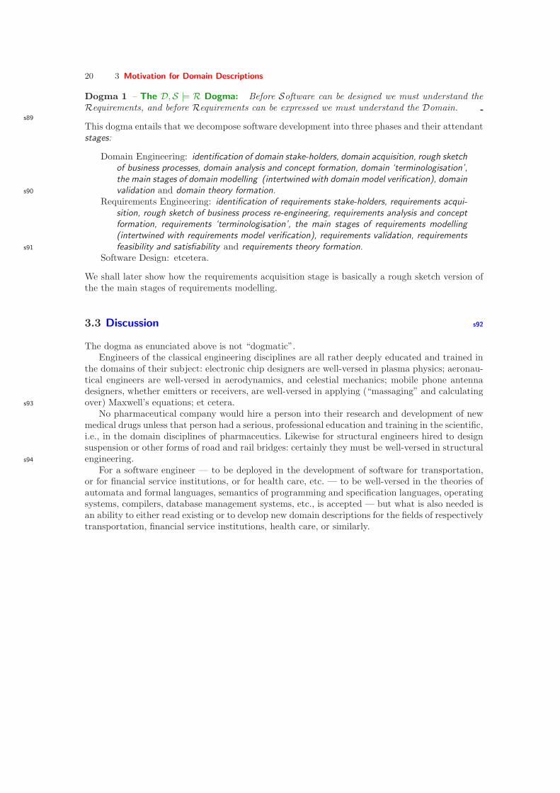
20 3 Motivation for Domain Descriptions
Dogma 1 – The D,S |= R Dogma: Before Software can be designed we must understand theRequirements, and before Requirements can be expressed we must understand the Domain.
s89
This dogma entails that we decompose software development into three phases and their attendantstages:
Domain Engineering: identification of domain stake-holders, domain acquisition, rough sketchof business processes, domain analysis and concept formation, domain ‘terminologisation’,the main stages of domain modelling (intertwined with domain model verification), domainvalidation and domain theory formation.s90
Requirements Engineering: identification of requirements stake-holders, requirements acqui-sition, rough sketch of business process re-engineering, requirements analysis and conceptformation, requirements ‘terminologisation’, the main stages of requirements modelling(intertwined with requirements model verification), requirements validation, requirementsfeasibility and satisfiability and requirements theory formation.s91
Software Design: etcetera.
We shall later show how the requirements acquisition stage is basically a rough sketch version ofthe the main stages of requirements modelling.
3.3 Discussion s92
The dogma as enunciated above is not “dogmatic”.Engineers of the classical engineering disciplines are all rather deeply educated and trained in
the domains of their subject: electronic chip designers are well-versed in plasma physics; aeronau-tical engineers are well-versed in aerodynamics, and celestial mechanics; mobile phone antennadesigners, whether emitters or receivers, are well-versed in applying (“massaging” and calculatingover) Maxwell’s equations; et cetera.s93
No pharmaceutical company would hire a person into their research and development of newmedical drugs unless that person had a serious, professional education and training in the scientific,i.e., in the domain disciplines of pharmaceutics. Likewise for structural engineers hired to designsuspension or other forms of road and rail bridges: certainly they must be well-versed in structuralengineering.s94
For a software engineer — to be deployed in the development of software for transportation,or for financial service institutions, or for health care, etc. — to be well-versed in the theories ofautomata and formal languages, semantics of programming and specification languages, operatingsystems, compilers, database management systems, etc., is accepted — but what is also needed isan ability to either read existing or to develop new domain descriptions for the fields of respectivelytransportation, financial service institutions, health care, or similarly.
Part III
Proper Conceptualisation


4
Abstraction & Modelling
s95 acm-aam
4.1 Abstraction
Abstraction relates to conquering complexity of description through the judicious use of abstrac-tion, where abstraction, briefly, is the act and result of omitting consideration of (what would thenbe called) details while, instead, focusing on (what would therefore be called) important aspects.
4.1.1 From Phenomena to Concepts s96
Phenomena are “things” that we can point to. They are often referred to as ‘individuals’ sincewhat is pointed to is a single specimen of possibly many “similar” instances of phenomena. We canthen, when “figuratively pointing to” an individual (a phenomenon), either keep “talking about”just that one individual, or we can ‘abstract’ to the class of all ‘similar’ phenomena. When we dothe latter then we have abstracted from a phenomenon, that is, a specific value, to a concept, i.e.,to the type of all such values.
4.1.2 From Narratives to Formalisations s97
We describe domains both informally, in terms of concise natural language narratives, and formally,using one or more formal specification languages. The terms of the natural language narrativedesignate concepts nouns typically denoting types and values of simple entities; verbs typicallydenoting operations over entities; etcetera. These terms are chosen carefully to correspond, as faras is reasonable in order to achieve a readable natural language text, to names of types, values,operations, etc., of the formal specification.Thus there is, in fact, a “two-way relation” between the s98
choice of mathematical abstractions of the formal specification and the terms of the narrative; theobjective is to bring “an as close as possible” relation between the narrative and the formalisation.
4.1.3 Examples of Abstraction s99
Example 10 illustrated two forms of abstraction: (i) model-oriented abstraction and (ii) property-oriented abstraction.
The model-oriented abstraction of Example 10 is illustrated by the modelling of nets as pairsof sets of hubs and links, cf. Item 2 on page 9: N = H-set × L-set, as well as by the concrete typesyntax types of link insertion and remove commands and their semantics, Items 9–24d (Pages 11–16).
The property-oriented abstraction of Example 10 is illustrated by the sorts and observersrelating to hubs and links, cf. Items 1 on page 9, 3–8 (Pages 10–11).
In this section we shall give some small examples of abstractions. s100

24 4 Abstraction & Modelling
Example 11 – Model-oriented Directory:
25. Terminal directory entries are files and files are further undefined.26. A directory consists of a finite set of uniquely (directory identifier) distinguished entries.27. A directory is either a file or is a directory.
type25. FILE, DId26. DIR = Did →m Entry27. Entry = FILE | DIR
Directories are modelled as maps. The specification abstracts from representation of directory identifiersand files.
s101
Example 12 – Networked Social Structures: People live in communities. People of communitiesmay network with people of distinct other communities. And people of such network may network withpeople of distinct other networks. We formulate this in a narrative and we formalise the narrative.s102
28. People are at the heart of any social structure.29. A region consists of a finite set of one or more communities and a finite set of zero, one or more
social networks.30. A community consists of a non-empty, finite set of people.31. A social network consists of a non-empty, finite set of two or more people, such that
a) all people of a network belong to distinct communities of the region, (i.e., no two people of anet belong to the same community),
b) and, if they also are members of other networks, then they all belong to distinct other networks(i.e., no two people of a network belong to the same other networks),
s103
type28. P29. R′ = C-set × N-set, R = |(cs,ns):R′
•cs 6=|30. C′ = P-set, C = |c:C′
•c 6=|31. N′ == mkN(sn:P-set), N = |mkN(ps):N′
•card ps≥2|axiom∀ (cs,ns):R •
31a. ∀ n:N • n ∈ ns ⇒card n = cardc|c:C•c ∈ cs ∧ n ∩ c 6= ∧
31b. ∃ p:P • p ∈ n ∧∃ n′:N • n′ ∈ ns ∧ n 6=n′ ∧ p ∈ n′ ⇒∀ p:P • p ∈ n ⇒∃ n′′:N • n′′ ∈ ns ∧ n 6=n′′ ∧ p ∈ n′′ ∧
card n′ = cardn′′|n′′:N•n′′ ∈ ns ∧ n′′ ∩ n′ 6= s104
Formula line cardn=cardc|c:C•c∈cs∧n∩c 6=, the first of the two lines starting with card, expressesthat the number of persons in the network is the same as the number of the communities to whichthese persons belong. The fact that n∩c 6= can be proven to be the same as card(n∩c)=1 is left asan exercise.
Formula line cardn′=cardn′′|n′′:N•n′′∈ns∧n′′∩ n′6=, the second of the two lines starting withcard, expresses that the number of persons in the network for the case that at least one of the personsin the network is a member of some other network, is the same as the number of the networks towhich all other persons of the n must belong. The fact that n′′∩n′ 6= can be proven to be the sameas card(n′′∩n′)=1 is left as an exercise.
s105
Example 13 – Railway Nets: We bring a variant of Example 10.

4.1 Abstraction 25
32. A railway net consists of one or more lines and two or more stations.
type32. RN, LI, ST
value32. obs LIs: RN → LI-set32. obs STs: RN → ST-set
axiom32. ∀ n:RN • card obs LIs(n) ≥ 1 ∧ card obs STs(n) ≥ 2
s10633. A railway net consists of rail units.
type33. U
value33. obs Us: RN → U-set
34. A line is a linear sequence of one or more linear rail units.
axiom34. ∀ n:RN, l:LI • l ∈ obs LIs(n) ⇒ lin seq(l)
s10735. The rail units of a line must be rail units of the railway net of the line.
value34. obs Us: LI → U-set
axiom35. ∀ n:RN, l:LI • l ∈ obs LIs(n) ⇒ obs Us(l) ⊆ obs Us(n)
36. A station is a set of one or more rail units.
value36. obs Us: ST → U-set
axiom36. ∀ n:RN, s:ST • s ∈ obs STs(n) ⇒ card obs Us(s) ≥ 1
s10837. The rail units of a station must be rail units of the railway net of the station.
axiom37. ∀ n:RN, s:ST • s ∈ obs STs(n) ⇒ obs Us(s) ⊆ obs Us(n)
38. No two distinct lines and/or stations of a railway net share rail units.
axiom38. ∀ n:RN,l,l′:LI•l,l′⊆obs LIs(n)∧l 6=l′⇒obs Us(l)∩ obs Us(l′)=38. ∀ n:RN,l:LI,s:ST•l ∈ obs LIs(n)∧s ∈ obs STs(n)⇒obs Us(l)∩ obs Us(s)=38. ∀ n:RN,s,s′:ST•s,s′⊆obs STs(n)∧s 6=s′⇒obs Us(s)∩ obs Us(s′)=
s10939. A station consists of one or more tracks.
type39. Tr
value39. obs Trs: ST → Tr-set
axiom39. ∀ s:ST•card obs Trs(s)≥1
40. A track is a linear sequence of one or more linear rail units.

26 4 Abstraction & Modelling
axiom40. ∀ n:RN,s:ST,t:Tr•s ∈ obs STs(n)∧t ∈ obs Trs(s)⇒lin seq(t)
s11041. No two distinct tracks share rail units.
axiom41. ∀ n:RN,s:ST,t,t′:Tr•s ∈ obs STs(n)∧t,t′⊆obs Trs(s)∧t 6=t′⇒obs Us(t) ∩ obs Us(t′)=
42. The rail units of a track must be rail units of the station (of that track).
value42. obs Us: Tr → U-set
axiom42. ∀ rn:RN,st:ST,tr:TR •
st ∈ obs STs(rn)∧tr ∈ obs Trs(st)⇒obs Us(tr)⊆obs Us(st)
s11143. A rail unit is either a linear, or is a switch, or a is simple crossover, or is a switchable crossover,
etc., rail unit.
value43. is Linear: U → Bool43. is Switch: U → Bool43. is Simple Crossover: U → Bool43. is Switchable Crossover: U → Bool
44. A rail unit has one or more connectors.
type44. K
value44. obs Ks: U → K-set
s11245. A linear rail unit has two distinct connectors. A switch (a point) rail unit has three distinct con-
nectors. Crossover rail units have four distinct connectors (whether simple or switchable), etc.
axiom∀ u:U •
is Linear(u) ⇒ card obs Ks(u)=2∧is Switch(u) ⇒ card obs Ks(u)=3∧is Simple Crossover(u) ⇒ card obs Ks(u)=4∧is Switchable Crossover(u) ⇒ card obs Ks(u)=4
46. For every connector there are at most two rail units which have that connector in common.
axiom46. ∀ n:RN • ∀ k:K • k ∈ ∪obs Ks(u)|u:U•u ∈ obs Us(n)
⇒cardu|u:U•u ∈ obs Us(n)∧k ∈ obs Ks(u)≤2
s11347. Every line of a railway net is connected to exactly two distinct stations of that railway net.
axiom47. ∀ n:RN,l:LI • l ∈ obs LIs(n) ⇒∃ s,s′:ST • s,s′ ⊆ obs STs(n) ∧ s 6=s′ ⇒
let sus=obs Us(s),sus′=obs Us(s′),lus=obs Us(l) in∃ u,u′,u′′,u′′′:U • u ∈ sus ∧
u′ ∈ sus′ ∧ u′′,u′′′ ⊆ lus ⇒let sks = obs Ks(u), sks′ = obs Ks(u′),

4.1 Abstraction 27
lks = obs Ks(u′′), lks′ = obs Ks(u′′′) in∃!k,k′:K•k 6=k′∧sks ∩ lks=k∧sks′ ∩ lks′=k′
end end
s11448. A linear sequence of (linear) rail units is an acyclic sequence of linear units such that neighbouring
units share connectors.
value48. lin seq: U-set → Bool
lin seq(us) ≡∀ u:U • u ∈ us ⇒ is Linear(u) ∧∃ q:U∗
• len q = card us ∧ elems q = us ∧∀ i:Nat • i,i+1 ⊆ inds q ⇒ ∃ k:K • obs Ks(q(i)) ∩ obs Ks(q(i+1)) = k ∧len q > 1 ⇒ obs Ks(q(i)) ∩ obs Ks(q(len q)) =
This ends Example 13s115
Example 14 – A Telephone Exchange:The example is “borrowed” — in edited form — from J.C.P. Woodcock and M. Loomes’ book
Software Engineering Mathematics [146]1
We start the informal description by presenting a synopsis and its immediate analysis: s116
• Synopsis: The simple telephone exchange system serves to efficiently honour requests for con-ference calls amongst any number of subscribers, whether immediately connectable, whereby theybecome actual, or being queued, i.e., deferred (or pending) for later connection. s117
• Analysis: The concepts of subscribers and calls are central: In this example we do not furtheranalyse the concept of subscribers. A call is either an actual call, involving two or more subscribersnot involved in any other actual calls, or a call is a deferred call, i.e., a requested call that is notactual, because one or more of the subscribers of the deferred call is already involved in actual calls.We shall presently pursue the concepts of requested, respectively actual calls, and only indirectlywith deferred calls.
s118
The structure of the types of interest are first described. We informally describe first the basis types,then their composition. (i) Subscribers: There is a class (S) of further undefined subscribers. (ii)Connections: There is a class (C) of connections. A connection involves one subscriber, the ‘caller’,and any number of one or more other subscribers, the ‘called’. (iii) Exchange: At any time an exchange s119
reflects (i.e., is in a state which records) a number of requested connections and a number of actualconnections (a) such that no two actual connections share any subscribers, (b) such that all actualconnections are also requested connections, and (c) such that there are no requested calls that arenot actual and share no subscribers in common with any other actual connection. (That is: The actualconnections are all that can be made actual out of the requested connections. This part addresses theefficiency issue referred to above.) (iv) Requested connections: The set of all requested connections for s120
a given exchange forms a set of connections. (v) Actual connections: The set of all actual connections,for a given exchange, forms a subset of its requested connections such that no two actual connectionsshare subscribers.
In this example we shall also be able to refer to the exchange, later to be named X, as ‘the state’(of the telephone exchange system). We shall later have a great deal more to say about the conceptof state.
1Permission to “lift” this example (converting it, however, from Z into RAISE, and providing it witha property-oriented solution) has been granted by Prof., Dr J.C.P. Woodcock (February 28, 2001).

28 4 Abstraction & Modelling
Formalisation of Property-oriented State s121
typeS, C, X
valueobs Caller: C → Sobs Called: C → S-setobs Requests: X → C-setobs Actual: X → C-set
subs: C → S-setsubs(c) ≡ obs Caller(c) ∪ obs Called(c)
subs: C-set → S-setsubs(cs) ≡ ∪ subs(c) | c:C • c ∈ cs
s122The overloaded function name subs stands for two different functions. One observes (“extracts”) theset of all subscribers said to be engaged in a connection. The other likewise observes the set of allsubscribers engaged in any set of connections. We shall often find it useful to introduce such auxiliaryfunctions.s123
axiom[ 1 ] ∀ c:C, ∃ s:S •
[ 2 ] s = obs Caller(c) ⇒ s 6∈ obs Called(c),
[ 3 ] ∀ x:X •
[ 4 ] let rcs = obs Requests(x),[ 5 ] acs = obs Actual(x) in[ 6 ] acs ⊆ rcs ∧[ 7 ] ∀ c,c′:C • c 6= c′ ∧ c,c′ ⊆ acs ⇒[ 8 ] obs Caller(c) 6= obs Caller(c′) ∧[ 9 ] obs Called(c) ∩ obs Called(c′) = ∧[ 10 ] ∼∃ c:C • c ∈ rcs \ acs •
[ 11 ] subs(c) ∩ subs(acs) = end
Let us annotate the above specification. [1] For all connections there exists a subscriber such that [2]the subscriber is a caller, but not a called subscriber. [3] For all telephone exchanges (i.e., telephoneexchange states), [4–5] let us observe the requested and the actual connections. [6] The actual onesmust also be requested connections, and [7] for any two different actual connections, [8] their callersmust be different, [9] the callers and the ones called cannot share subscribers, and [10] there must notbe a requested, but not actual connection [11] which could be an actual connection. That is all suchconnections must have some subscriber in common with some actual connection.s124
The last two lines above express the efficiency criterion mentioned earlier.We can express a law that holds about the kind of exchanges that we are describing:
theorem∀ x:X •
obs Actual(x)= ≡ obs Requests(x)=s125
The law expresses that there cannot be a non-empty set of deferred calls if there are no actual calls.That is, at least one deferred call can be established should a situation arise in which a last actual callis terminated and there is at least one deferred call.
The law is a theorem that can be proved on the basis of the telephone exchange system axiomsand a proof system for sets.

4.1 Abstraction 29
Operation Signatures s126
The following operations, involving telephone exchanges, can be performed: (i) Request: A caller indi-cates, to the exchange, the set of one or more other subscribers with which a connection (i.e., a call)is requested. If the connection can be effected then it is immediately made actual, else it is deferredand (the connection) will be made actual once all called subscribers are not engaged in any actualcall. (ii) Caller Hang: A caller, engaged in a requested call, whether actual or not, can hang up, i.e.,terminate, if actual, and then on behalf of all called subscribers also, or can cancel the requested (butnot yet actual) call. (iii) Called Hang: Any called subscriber engaged in some actual call can leave s127
that call individually. If that called subscriber is the only called subscriber (“left in the call”), then thecall is terminated, also on behalf of the caller. (iv) is Busy: Any subscriber can inquire as to whetherany other subscriber is already engaged in an actual call. (v) is Called: Any subscriber can inquire asto the identities of all those (zero, one or more) callers who has requested a call with the inquiringsubscriber. s128
First the signatures:
valuenewX: Unit → Xrequest: S × S-set → X → X
caller hang: S → X∼→ X
called hang: S → X∼→ X
is busy: S → X → Boolis called: S → X → Bool
s129The generator function newX is an auxiliary function. It is needed only to make the axioms cover allstates of the telephone exchange system. In a sense it generates an empty, that is, an initial state.Usually such empty state generator functions are “paired” with a similar test for empty state observerfunction. s130
Then we get the axioms:
axiom∀ x:X • obs Requests(x)= ≡ x=newX(),∀ x:X,s,s′:S,ss:S-set •
∼is busy(s,newX()) ∧s 6=s′ ⇒
s ∈ ss ⇒ is busy(s)(request(s′,ss)(x)) ∧s 6∈ ss ⇒ is busy(s)(request(s′,ss)(x)) ≡ is busy(s)(x),... etcetera ...
s131We leave the axiom incomplete. Our job was to illustrate the informal and formal parts of a property-oriented specification, not to do it completely.
Model-oriented State s132
typeSC = | ss | ss:S-set • card ss ≥ 2 |R = C-setA = C-setX = | (r,a) | (r,a):R×A • a ⊆ r ∧ ⋂
a = |

30 4 Abstraction & Modelling
Efficient States s133
There is a notion of telephone exchange system efficiency, a constraint that governs its operation,hence the state, at any one time. The efficiency criterion says that all requested calls that can actuallybe connected are indeed connected:
value
eff X: X∼→ Bool
eff X(r,a) ≡ ∼∃ a′:A • a ⊂ a′ ∧ (r,a′) ∈ X
Formalisation of Action Types s134
typeCmd = Call | Hang | BusyCall′ == mk Call(p:S,cs:C)Call = | c:Call′ • card cs(c) ≥ 1 Hang == mk Hang(s:S)Busy == mk Busy(s:S)
Pre/Post and Direct Operation Definitions s135
We shall, for each operation, define its meaning both in terms of pre/post conditions and in terms ofa direct “abstract data type algorithm”.
Multi-party Call s136
A multi-party call involves a (primary, s) caller and one or more (secondary, ss) callees. Enacting sucha call makes the desired connection a requested connection. If none of the callers are already engagedin an actual connection then the call can be actualised. A multi-party call cannot be made by a callerwho has already requested other calls.s137
value
int Call: Call∼→ X
∼→ Xint Call(mk Call(p,cs))(r,) as (r′,a′)pre p 6∈ ⋃
rpost r′ = r ∪ p ∪ cs ∧ eff X(r′,a′)
int Call(mk Call(p,cs))(r,a) ≡let r′ = r ∪ p ∪ cs,
a′ = a ∪ if (p ∪ cs ∩ ⋃a) =
then p ∪ cs else end in(r′,a′) endpre p 6∈ ⋃
r
The above pre/post-definition (of int Call) illustrates the power of this style of definition. No algo-rithm is specified, instead all the work is expressed by appealing to the invariant!
Call Termination s138
It takes one person, one subscriber, to terminate a call.

4.2 Modelling 31
value
int Hang: Hang → X∼→ X
int Hang(mk Hang(p))(r,a) as (r′,a′)pre existS c:C • c ∈ a ∧ p ∈ apost r′ = r \ c|c:C • c ∈ r ∧ p ∈ c ∧ eff X(r′,a′)
int Hang(mk Hang(p))(r,a) ≡let r′ = r \ c | c:C • c ∈ a ∧ p ∈ c ,
a′ = a \ c | c:C • c ∈ r ∧ p ∈ c inlet a′′ = a′ ∪ c | c:C • c ∈ r′ ∧ c
⋂a′ = in
(r′,a′′) end endpre existS c:C • c ∈ a ∧ p ∈ a
The two ways of defining the above int Hang function again demonstrate the strong abstractionalfeature of defining by means of pre/post-conditions.
Subscriber Busy s139
A line (that is, a subscriber) is only ‘busy’ if it (the person) is engaged in an actual call.
value
int Busy: S → X∼→ Bool
int Busy(mk Busy(p))( ,a) as bpre truepost if b then p ∈ ⋃
a else p 6∈ ⋃a end
int Busy(mk Busy(p))( ,a) ≡ p ∈ ⋃a
Here, perhaps not so surprisingly, we find that the explicit function definition is the most straightforward.This ends Example 14
4.1.4 Mathematics and Formal Specification Languages s140
Using mathematical concepts has shown to be the most powerful way of expressing abstractions.The discrete mathematical concepts of sets, Cartesians, sequences, maps, that is, enumerablefunctions and functions, as well as mathematical logic and algebras has served mathematicianswell for quite some time and will serve professional software engineers well. s141
Formal specification languages, like Alloy [90], Event B [1, 33], RSL [17–19, 61, 62, 64], VDM[26, 27, 55, 56], Z [77, 78, 137, 138, 145] and others, embody the above-mentioned mathematical
concepts in quite readable forms. The current book favours the RAISE specification language RSL.The first use of the RSL notation was in Example 10 starting Page 9. That first use of RSL will beextensively annotated and with margin references to sections and pages of Appendix A.
4.2 Modelling s142
Definition 7 Model: A model is the mathematical meaning of a description of a domain, or aprescription of requirements, or a specification of software, i.e., is the meaning of a specificationof some universe of discourse.
s143
Definition 8 Modelling: Modelling is the act (or process) of identifying appropriate phenomenaand concepts and of choosing appropriate abstractions in order to construct a model (or a set ofmodels) which reflects appropriately on the universe of discourse being modelled.

32 4 Abstraction & Modelling
4.2.1 Property-oriented Modelling s144
Definition 9 Property-oriented Modelling: By property-oriented modelling we shall under-stand a modelling which emphasises the properties of what is being modelled, through suitable useof abstract types, that is, sorts, of postulated observer (obs ), generator (mk ) and type checking( is ) functions, and axioms over these.
4.2.2 Model-oriented Modelling s145
Definition 10 Model-oriented Modelling: By abstract, but model-oriented modelling we shallunderstand a modelling which expresses the properties of what is being modelled, through suitableuse of mathematical concepts such as sets, Cartesians, sequences, maps (finite domain, enumerablefunctions), and functions (in the sense of λ-Calculus functions).
4.3 Model Attributes s146
Specifications achieve their intended purpose by emphasising one or more attributes. Either: (i.1)analogic, (i.2) analytic and/or (i.3) iconic; and then either: (ii.1) descriptive or (ii.2) prescriptive;and finally either: (iii.1) extensional or (iii.2) intensional. That is, a model may, at the sames147
time (although time has nothing to do with this aspect of models), be one or more of analogic,analytic and iconic; expressed either only descriptive, or mostly descriptive (with some prescriptiveaspects), or only prescriptive, or mostly prescriptive (etc.); and expressed either only extensional,or mostly extensional (with some aspects), or only intensional, or mostly intensional (etc.). Wemay claim that a good model blends the above consciously and judiciously — including featuringexactly (or primarily) one attribute from each of the three categorisations. We next take a lookat these model attributes.
4.3.1 Analogic, Analytics and Iconic Models s148
Definition 11 Analogic Model: An analogic model resembles some other universe than the uni-verse of discourse purported to be modelled.
Definition 12 Analytic Model: An analytic model is a mathematical specification: It allowsanalysis of the universe of discourse being modelled.
Definition 13 Iconic Model: An iconic model is an “image” of the universe of discourse that isthe target of our attention.
s149
Example 15 – Analogic, Analytic and Iconic Models: We lump three kinds of examples intoone larger example:
• Analogic models: (1) The symbol, on the visual display screen of your computer, of a trash can,denoting an ability to delete files.2 (2) A four-pole, electric circuit network of resistors, inductances,capacitors and current or voltage supplies can be used to analogically model some aspects of thebehaviour of certain mechanical vibration and/or spring dampening aggregations. (3) A tomographicimage of, say the brain, with its colour-enhanced “blots” is an analogic model of a cross section ofthat brain!s150
2Thus Macintosh systems, although undoubtedly so-called “user-friendly”, got the concept namewrong: The Macintosh ‘trash can’ symbol is not an icon! It is an analogic!

4.3 Model Attributes 33
• Analytic models: (4) The differential equations whose variables model spatial x, y, z coordinatesand the temporal t dimension, and whose constant, m, model the mass of a stone, may be ananalytic model of the dynamics of the throwing of such a stone in a vacuum. (5) A description,in RSL, involving quantities that purport to model bank accounts, their balance, time, etc., maybe an analytic model of a banking system — in the real world — provided the model reflects atleast “some of the things that can go wrong” in actual life. (6) A graph with labelled nodes andweighted arcs may be used as a model of a road net with cities and distances between these, andcan be used for the computation of shortest distances, etc. s151
• Iconic models: Typical iconic models are certain advisory or judicially binding traffic signs: (7) Theroadside sign showing, typically in Sweden, an Elk, denoting that elks may be crossing the roadahead at any time; (8) the roadside sign showing an automobile (from behind) "underlined"
with two crossing S curves, denoting that the road surface ahead may be slippery and hencethat automobiles may spin out of control; and (9) the roadside sign showing a crossed-out horn,denoting that use of the automobile horn is not allowed.
Observe that a model may possess characteristics of more than one of the above attributes.
4.3.2 Descriptive and Prescriptive Models s152
Definition 14 Descriptive Model: A descriptive model 3 describes something already existing.
Definition 15 Prescriptive Model: A prescriptive model 4 models something as yet to be im-plemented.
s153
Thus domain specifications are descriptive, while requirements specifications are prescriptive. A re-quirements specification prescribes properties that the intended software (cum computing system)shall satisfy. A software specification prescribes certain kinds of computations. s154
We remind the reader that we use the terms model and specification near synonymously. Aspecification defines a set of zero, one or more, possibly even an infinity, of models. But we usethe term the model in connection with a given specification to stand for the general member ofthe set of models. Hence when we use the term model below, please read specification. s155
Example 16 – Descriptive and Prescriptive Models: A descriptive model: A railway net consistsof two or more distinct stations and one or more distinct railway lines. A railway line consists of alinear sequence of one or more linear rail units. Any railway line connects exactly two distinct stations.A route is a sequence of one or more, and if more, then connected railway lines. Two railway lines areconnected if they have the connecting station in common. s156
A prescriptive model: The train timetable shall, for each train journey, list all station visits. A traintimetable station visit shall list the name of the station visited, the time of arrival of the train, the timeof departure of the train. No train timetable train journey entry lists the same station twice. Timesof train departures and train arrivals shall be compatible with reasonable stops at stations and withthe distance between stations visited. Two immediately time-consecutive train timetable station visitsmust be compatible with the railway net: It shall be possible to route a train between such consecutivestations.
s157
Notice in the descriptive model the unhedged use of the verbs consists, connects, is and are. Adescription is indicative: 5 It tells what there is. Likewise notice in the prescriptive model the useof the (compelling) verbs shall and must. A prescription is putative: 6 It tells what there will be.
3Descriptive: factually grounded or informative rather than normative, prescriptive, or emotive [139].4Prescriptive: to lay down a rule [139].5Indicative: of, relating to, or constituting a verb form or set of verb forms that represents the denoted
act or state as an objective fact [139].6Putative: of “putare” to think, assumed to exist [139].

34 4 Abstraction & Modelling
4.3.3 Extensional and Intensional Models s158
Definition 16 Extensional Model: An extensional model 7 (black, opaque box) presentationmodels something as if observed by someone external to the universe of discourse.
Definition 17 Intensional Model: An intensional model 8 in logic, correlative words that in-dicate the reference of a term or concept. Intension indicates the internal content of a term orconcept that constitutes its formal definition. .
s159
Intensional versus extensional meaning: (i) intensional meaning: consists of the qualities or at-tributes the term connotes (the attributes of class membership); (ii) extensional meaning: consistsof the qualities or attributes the term denotes (the class members themselves).
Connotation: the suggesting of a meaning by a word apart from the thing it explicitly namesor describes.
Denotation: a direct specific meaning as distinct from an implied or associated idea. (glass (orwhite), transparent box) presentation models the internal structure of the universe of discourses160
An extensional model presents, i.e., reflects, the behaviour as seen from an outside. In that senseone may claim, but the claim cannot be justified from extensionality alone, that an extensionalmodel focuses on properties, on what the thing that is being modelled offers an outside world, i.e.,users of that thing. If a model is expressed in a property-oriented style, then we can claim theconverse: that the model is extensional!
An intensional model presents the internal mechanisms of what is being modelled in a waythat may explain why it has the extension that it might have.s161
The subject of intension and extension, in mathematical logic as well as in philosophy, is not aclosed book. It is still very much subject to analysis, redefinition, rethinking. In this paper we shallrestrict ourselves to the views expressed above. Extension is the “black box” view of observingonly externally perceivable properties of what is being specified. Intension is the “glass box” viewof observing some, most or all of the inner workings of what is being specified.
Example 17 – Extensional Model Presentations: (1) To explain the square root function,√
n =r, by explaining that r × r = n ∧ r ≥ 0 is to give an extensional definition, hence model.
(2) To explain a stack extensionally we may define (a) the stack sorts for elements and stacks, (b)the signatures of the empty, pop, top and push functions, and (c) the axioms which relate sorts andoperations.
s162
Example 18 – Intensional Model Presentations: (1) To explain the square root function,√
n,by presenting, e.g., the Newton–Raphson algorithm ([121] pp. 230, 347, 355 and 360), is to give anintensional definition, hence model.
(2) An intensional model of stacks may model stacks as lists of (extensionally modelled) elements,and define the (i) empty, (ii) pop, (iii) top, and (iv) push functions in terms of (i) constructing theempty list, of (ii) yielding the tail of a list, of (iii) yielding the head element of a list, and (iv) ofconcatenating a supplied element to the front of the list.
4.4 Roles of Models s163
We pursue modelling for one or more reasons:(i) To gain understanding: in the process of modelling we are forced to come to grips with
many issues of the universe of discourse.(ii) To get inspiration and to inspire: abstraction often invites such generalisations that induce,
in the writer, or in the reader, desires of change.(iii) To present, educate and train: a model can serve as the basis for presentations to others
for the purposes of awareness, education or training.s164
7Extensional: concerned with objective reality.8Intensional: TBD

4.5 Exercises 35
(iv) To assert and predict: a mathematical, including a formal model, usually allows abstractinterpretation — in the “vernacular”: calculations, computations — that simulates, estimates orotherwise expresses potential properties of the universe of discourse.
(v) To implement: two kinds of implementations can be suggested: in business process re-engineering we propose the re-engineeringof some domain on the basis of a model and in computingsystems design we base the development of requirements on a domain specification and we basesoftware design on requirements.
4.5 Exercises
See Items 3–4 (of Appendix D, starting Page 230).


5
Semiotics
s165 acm-semiotics
5.1 An Overview
The following decomposition of language concepts and their explication is taken from [6]. Thesyntax-semantics-pragmatics sub-structuring is believed to be due to Morris [34–36,108,109,147].In fact, the term ‘semiotics’, as we use it, is really to be taken in its widest meaning [37].
Definition 18 – Semiotics: Semiotics is the study of and knowledge about the structure of all‘sign systems’. We divide this study (and our knowledge) into three parts: syntax, semantics andpragmatics.
Conventional natural language as spoken (written) by people is but one ‘sign’ system. Examplesof sign systems are sound (audio), sight (visual), touch (tactile), smell and taste — and in allcontexts: dance, film, politics, eating and clothing [37]. s166
Definition 19 – Syntax: Syntax is the study of and knowledge about how signs (words) can beput together to form correct sentences and of how sentence-signs relate to one another.
We shall understand signs (words) and sentences in a wide sense. Programs in a programing lan-guages and specifications in a formal specification language will here be considered to be sentences.and variable and function identifiers (a, ab, id, fct, etc.); constants (0, 1, 2, . . . , true, false, chaos,etc.); expressions and statements; statement and expression symbols (such as value operators s167
(+,−, /, ∗,×, 7→, etc.), and dom, rng, elems, len, card) etc.; type operators (Boolean, integer,
real, char, string, etc., and -set, -infset, ∗, ω, →,∼→, →m , ×); parentheses ((, ), , , [, ] etc.);
comma (,); semicolon (;); assignment symbols (:=, =, ←); definition symbols (≡, ::=) etc.) andliterals (such as begin, end, let, in, cases, of, while, do, type, value, axiom, etc.) will here beconsidered words. s168
But also diagrams, say technical drawings and actual layout of, for example, buildings andrailway tracks, will be considered sentences, and the boxes and lines of diagrams, and the variousvisual (proper) sub-components of actual physical phenomena will be considered words. That is, we s169
consider phenomena such as geographical and geodetic maps; buildings, and their “accompanying”architectural and engineering drawings; railway tracks (lines and stations) and their “accompany-ing” engineering drawings; cities and city plans; etc., as languages [5]. GIS and CAD/CAM systemsthus translate descriptions of such phenomena into database structures and GIS and CAD/CAMsystem user commands are compiled and executed as language programs in the context of thesedatabases. s170
We define syntaxes in terms of either BNF grammars or RSL types. We distinguish between syn-tactic types and semantic types. The syntactic types designate sentences and words. The semantictypes designate meanings (of sentences and words).

38 5 Semiotics
Definition 20 – Semantics: Semantics is the study of and knowledge about the meaning ofwords, sentences, and structures of sentences.
s171
Let
typeSynType, SemType
designate syntactic, respectively semantic types. Then
valueM: SynType → SemType
presents the signature of a semantic function M. It assumes all syntactic inputs to be well-formed.If the syntax of SynType is such as to allow ill-formed sentences, then we must define a well-formedness function:
valueWf SynType: SynType → Bool
and the signature of M must be sharpened:
value
M: SynType∼→ SemType
s172
Definition 21 – Pragmatics: Pragmatics is the study of and knowledge about the use of words,sentences and structures of sentences, and of how contexts affect the meanings of words, sentences,etc.
5.2 Syntax s173
We recall our definition: syntax is the study of and knowledge about how signs (words) can beput together to form correct sentences and of how sentence-signs relate to one another.
We shall divide our presentation of syntax into three parts: (i) BNF grammars, (ii) concretetype syntax and (iii) abstract type syntax. These three are just three increasingly more abstractways of dealing with syntax.s174
The subject of syntax goes well beyond our software engineering treatment. The computerscience topic of formal languages and automata theory studies far wider consequences of gram-mars and syntax than we cover. Seminal books are [83]1 The computing science topic of regularexpression recognizers and context free language parsers likewise goes well beyond our coverage —and their study is important for the software engineer to implement efficient software for languagehandling. Seminal books are [4].2s175
BNF grammars define sets of strings of characters; concrete type syntaxes define sets of math-ematical structures (numbers, Booleans, sets, Cartesians, maps and functions over concrete typevalues); and abstract type syntaxes define properties of simple phenomena and concept entities.We say that BNF grammars and concrete type syntaxes define simple phenomena and conceptentities in a model-oriented fashion whereas abstract type syntaxes define simple phenomena andconcept entities in a property-oriented fashion.
1 Dines: Find more recent references.2 Dines: Find more recent references.

5.2 Syntax 39
5.2.1 BNF Grammars s176
BNF stands for Backus Naur Form. BNF grammars, as we shall see, stand for sets of finite lengthstrings of characters, including blanks and punctuation marks.
Definition 22 – Character: A character is a symbol that can be displayed (on paper, on acomputer screen, or otherwise).
Example 19 – Characters: Our example is the conventional example of characters from an En-glish/American computer keyboard: a, A, b, B, c, C, ..., z, Z, 0, 1, 2, 3, 4, 5, 6, 7, 8, 9, !, @, #, $, %,&, *, ˜, (, ), , , [, ], -, +, ’, ”, <, >, ., ,, :, ;, ?, /, |, [blank], etc.
s177
Definition 23 – Alphabet: An alphabet is a finite set of characters.
Example 20 – Alphabet: Three examples, Ai,Aj ,Ak, of subsets of the above characters:
• Ai : a,b,[blank],O,|• Aj : a,b,c,d,e,f,g,h,i,j,k,l,m,n,o,p,q,r,s,t,u,v,w,x,y,z,[blank]• Ak : 0,1,2,3,4,5,6,7,8,9,[blank],a,b,c,d,e,f,g,h,i,j,k,l,m,n,o,p,q,r,s,t,u,v,w,x,y,z
s178
Definition 24 – Terminal: By a terminal we understand a sequence of one or more charactersof some given alphabet.
Example 21 – Terminals:
• a, b, c, 0, 1;• a, aa, aaa, abc, 0, 1, 00, 01, 001;• open, deposit, withdraw, close, account, client, number.
s179
Definition 25 – Non-terminal: By a non-terminal we understand a specially highlighted sequenceof one or more characters, not necessarily from the alphabet of a given set of terminals.
Example 22 – Non-terminals:
• <| Command>|,• <| Open>|, <| Deposit>|, <| Withdraw>|, <| Close>|• <| ClientName>|, <| AccountNumber>|,• <| Cash>|, <| Amount>|
s180
Definition 26 – BNF Rules: By a BNF rule we understand a triple: (L, ::=, As) where L isa non-terminal and As is a finite set of zero, one or more alternatives where an alternative is afinite sequence of zero, one or more non-terminals and/or terminals. ::= is the definition symbol.
Example 23 – BNF Rules:
• <| Command>| ::= <| Open>| | <| Close>|• <| Open>| ::= client <| ClientName>| opens account• <| Withdraw>| ::= client <| ClientName>| withdraws <| Amount>|
from account <| AccountNumber>|
s181
Definition 27 – BNF Grammar: By a BNF grammar we understand a quadruple
(N , T ,R,G)

40 5 Semiotics
• N is an alphabet of non-terminals,• T is an alphabet of terminals,
• R is a set of rules,• G is a non-terminal,
such that G is in N ; all the left hand sides of rules in R are in N ; all the non-terminals of righthand sides of rules in R are distinct and together form N ; and all the terminals of right handsides of rules in R are in T .
s182
Example 24 – BNF Grammar: Banks: The ... (Identifiers,Alphanumerics,Numerals) are not partof the syntax.
N : <| Command>|, <| Open>|, <| Deposit>|, <| Withdraw>|, <| Close>|, <| ClientName>|,<| AccountNumber>|, <| Amount>|
T : client,opens account,deposits,into account,withdraws,from account,closes account . . .... ∪ Identifiers ∪ Alphanumerics ∪ Numerals
R : <| Command>| ::= <| Open>| | <| Deposit>| | <| Withdraw>| | <| Close>|<| Open>| ::= client <| ClientName>| opens account<| Deposit>| ::= client <| ClientName>| deposits <| Amount>| into account <| AccountNumber>|<| Withdraw>| ::= client <| ClientName>| withdraws <| Amount>| from account <| AccountNumber>|<| Close>| ::= client <| ClientName>| closes account <| AccountNumber>|<| ClientName>| ::= ... Identifiers<| AccountNumber>| ::= ... Alphanumerics<| Amount>| ::= ... Numerals
G : <| Command>|
s183
The “... ∪ Identifiers ∪ Alphanumerics ∪ Numerals” which is not part of the syntax, ought befully defined by a somewhat longer BNF grammar.
The example showed one form of BNF grammars. In the below definition of the meaning ofBNF grammars we abstract from the above forms of rules for BNF grammars.
Examples 26 on the facing page and 28 on page 45 follow up on this example of a BNF grammarby presenting a concrete type syntax, respectively an abstract type syntax for “supposedly” thesame command language.s184
Definition 28 – Meaning of a BNF Grammar: The meaning of a BNF grammar is a language,that is, a possibly infinite set of finite length strings over the terminal alphabet of the BNF grammar.To properly define this language, for any BNF grammar we shall proceed, formally, as follows:
Let N and T denote the alphabets of non-terminals and terminals.Let r : (n, ℓ1, ℓ2, . . . , ℓm) designate a rule, r, that is: n : N and ℓi : (N |T )∗, for m ≥ 0, 1 ≤
i ≤ m where (N |T )∗ denotes the possibly infinite set of finite length strings over non-terminal andterminal characters.
Let G : (N, T, R, n0) where G names the grammar, N the alphabet of non-terminals, T thealphabet of terminals, R the finite set of rules (over N and T ), and n0 a distinguished non-terminalof N .
G is constrained as follows: no two distinct rules, (n, ls) and (n′, ls′) in G have n = n′, thatis: all left hand side non-terminals are distinct and together they form N , and there is a ruler : (n, ℓ1, ℓ2, . . . , ℓm) in R such that n = n0.s185
Let sisj denote the concatenation of strings si and sj.Let sUs′ be a string over (N |T )∗.Let (U, ℓ1, ℓ2, . . . , ℓi, . . . , ℓm) be a rule in R.Then sUs′ →G sℓis′ means: from sUs′, by means of rule (U, ℓ1, ℓ2, . . . , ℓm) of G,
we derive, →G, sℓis′.If, in some rule (U, ℓ1, ℓ2, . . . , ℓi, . . . , ℓm), m = 0, that is, the rule is (U, ), then sUs′ →G
ss′.

5.2 Syntax 41
If sp →G sq, sq →G sr, ..., and sv →G sw, then sp →G∗ sw (and thus sp →G
∗ sr, sp →G∗ sw,
etc. — assuming sp →G∗ sv).
The meaning of →G is specific to the given Grammar.Now the meaning, L(G) is defined as follows:
LG = s | n0 →G∗ s ∧ s ∈ T ∗
s186
Some BNF grammars are such that LG is empty: no derivation, →G, and hence →G∗, results in
terminal strings. s187
Example 25 – Meaning of a BNF Grammar: First we show a form of BNF grammar which ismore in line with the above definition.
N = E, C, V, P, I, B,T = 0, 1, 2, 3, 4, 5, . . . , a, b, c, . . . , z,+,−, ∗, /,R =0 E = C | V | P | I | B,1 C = 0 | 1 | 2 | 3 | 4 | 5 . . .,2 V = a | b | c | . . . | z,3 P = −E,4 I = E O E,5 O = + | − | ∗ | /,6 B = ( E ) n0 = E
s188
Then we show a derivation of the expression 5 + (a/3) +−c from E:
E → 0I → 4E O E → 0C O E → 15 O E → 55 + E → 05 + I → 45 + E O E → 65 + B O E → 45 + ( E ) O E → 05 + ( I ) O E → 4
5 + ( E O E ) O E → 05 + ( V O E ) O E → 25 + ( a O E ) O E → 55 + ( a / E ) O E → 05 + ( a / C ) O E → 15 + ( a / 3 ) O E → 55 + ( a / 3 ) + E → 05 + ( a / 3 ) + P → 35 + ( a / 3 ) + −E → 05 + ( a / 3 ) + − V → 25 + ( a / 3 ) + − c
s189
Please disregard that we have, in the above derivation, always replaced the leftmost non-terminal. Thatis of no consequence. The fact that the BNF grammar is ambiguous, that is, allows entirely distinctderivation sequences to lead to the same final string also should be disregarded. It is, at most, perhaps,an unfortunate choice of grammar !
5.2.2 Concrete Type Syntax s190
Definition 29 – Concrete Type Syntax: By a concrete type syntax we shall understand thedefinition of a set of mathematical structures such as sets, Cartesians, lists, maps and functions.
s191
Example 26 – A Concrete Type Syntax: Banks:
49. There are clients, c:C, account numbers a:A and money, m:M.50. A bank record client accounts and account balances.51. Client accounts map client names to a finite number of zero, one or more account numbers.

42 5 Semiotics
52. Account balances map account numbers into money balances.53. All client accounts are recorded by the account balances, and the account balances record only
accounts listed by one or more clients.
type49. C, A, Money50. Bank = Clients × Accounts51. Clients = C →m A-set52. Accounts = A →m Moneyaxiom53. ∀ (cs,acs):Bank • ∪ rng cs = dom acs
s192The two sentences of Item 53 (53.1) All client accounts are recorded by the account balances, and(53.2) the account balances record all accounts listed by clients. correspond to:
axiom53. ∀ (cs,acs):Bank •
53.1 ∪ rng cs ⊆ dom acs53.2 dom acs ⊆ ∪ rng cs
Hence formula line 53.s193
We then give a concrete type syntax for a bank/client comand language first hinted at in Example 24on page 40.
54. To the syntactic types we include client identifications, account numbers, money (i.e., cash) andamounts of such.
55. There are open, deposit, withdraw and close commands.56. Open commands identify the client.57. Deposit commands identify the client, the account number and the monies to be deposited.58. Withdraw commands identify the client, the account number and the amount of monies to be
withdrawn.59. Close commands identify the client and the account to be closed.
s194
54. C, A, Money, Amount55. Command = Open | Deposit | Withdraw | Close56. Open == mkO(c:C)57. Deposit == mkD(c:C,a:A,m:Money)58. Withdraw == mkW(c:C,a:A,amount:Amount)59. Close == mkC(c:C,a:A)
This example will be followed up by Examples 28 on page 45 and 29 on page 46.s195
Definition 30 – Meaning of Concrete Type Syntax: We explain both the syntactic RSL typedefinitions, expressions and their meaning. First the syntax.
60. There are two kinds of type definitions:a) simple type definitions which have a left hand side type name and a right hand side type
expression (separated by an equal sign: ‘=’),b) record type definitions which have a left hand side type name and a right hand side pair of a
record constructor name and a parenthesized list of pairs of distinct selector and not necessarilydistinct type names (where the left and the right is separated by a double equal sign: ‘==’).
61. Type, record constructor and selector names are identifiers.s196
62. A type expression is either

5.2 Syntax 43
a) a Boolean (Bool) orb) an integer number (Intg) orc) a natural number (Nat) ord) a real number (Real) type name, or ise) a set (A-set) orf) a Cartesian (A×B×. . .×C) or
g) a list (A∗) or
h) a map (A →m B) or
i) a partial (A∼
→B) or
j) a total function (A→B) type expression, or is
k) a set of (alternative, |) type expressions.
The below only shows how such type definitions and expressions may look like when we (otherwise)write them. That is, the below type definitions and expressions are not type definitions and propertype expressions. s197
Type Definition Examples:60a. TN = TE60b. TN == RN(s1:TN1,s2:TN2,...,sn:TNm)
Type Expression Examples:62. TE =62a. Bool62b. Int62c. Nat62d. Real
62e. TE-set62f. TE1×TE2×...×TEm62g. TE∗
62h. TEi →m TEj
62i. TEi∼
→ TEj62j. TEi → TEj62k. TE1 | TE2 | ... | TEm
where: m≥2
In an concrete type syntax of two or more type definitions all left hand side type names are distinct, alltype names occurring in right hand side record constructor and type expressions are defined by an abstractor concrete type syntax, and no set (62e.) or function (62h.,62i.) type is defined recursively. Now to the s198
meaning of a concrete type syntax.
• The meaning of a type name is the meaning of the right hand side⋆ type expression TE⋆ or record constructor expression RN(s1:TN1,s2:TN2,...,sn:TNm).
We shall use a concept of the meanings being “sets” of values. The practicing software engineer mayconsider these “sets” just as normal set. But, for reasons not explained here, but based in a properdefinition of a mathematical semantics for RSL, they are not sets in the usual sense of mathematics. s199
• The meaning of a type expression depends on its form:⋆ Bool: the “set” false,true,chaos;⋆ Intg: the “set” of all integers: . . . ,-3,-2,-1,0,1,2,3,. . . ;⋆ Nat: the “set” of all natural numbers 0,1,2,3,. . . ;⋆ Real: the “set” of all real number m/n | m,n :Nat, n 6= 0;⋆ TE-set: the “set” of all finite sets of zero, one or more elements, ei, of TE: . . . ei, ej , . . . , ek. . . ;⋆ TE1×TE2×...×TEm: the “set” of all Cartesians . . . , (eTE1i
, eTE2i, . . . , eTEmn), . . . ;
⋆ TE∗: the “set” of all finite length sequences (or lists) of zero, one or more elements, ei, of TE:. . . ,〈ei, ej , . . . , ek〉,. . . ;
⋆ TEi →m TEj: the “set” of all finite maps (that is, finite definition set discrete functions) fromelements, eik
, of TEi to elements, ejℓ, of TEj: . . . ,[. . . ,eik
7→ejℓ,. . . ]. . . ; s200
⋆ TEi∼
→TEj: the “set” of all partial functions from some, but not all elements, eik, of TEi, to elements,
ejℓ, of TEj: λei : TEi • ETEj;
3
⋆ TEi→TEj: the “set” of all total functions from elements eik, of type TEi, to elements, ejℓ
, of TEj:λei • Ej ; and
⋆ TE1|TE2|...|TEm: the “set” which is a “union” of the “sets” denoted by the TEi for i=1,2,. . . ,m.• The meaning of a record constructor type definition, Tn == RN(s1:TN1, s2:TN2, ..., sn:TNm), is the
“set” of all records, . . . , RN(te1,te2,. . . ,tem), . . . , where tei is any value of type TEi for all i.
s201
Where the meaning of a BNF grammar is a possibly infinite set of strings over a terminal alphabet,the meaning of a concrete type syntax is a possibly infinite “set” of mathematical values: Booleans,numbers, sets, Cartesians, lists, maps, partial and total functions, where the elements of sets,Cartesians, lists and maps, and where the function argument and results values are any of thevalues of any of these mathematical values.
The RSL type constructs also allow infinite sets, TE-infset, and infinite length lists, TEω.
3The expression λe : Ti • ETjdenotes the function which when applied to elements v, of type Ti, yields
a value (of type Tj) of expression ETjwhere all free occurrences of e are replaced by v.

44 5 Semiotics
5.2.3 Abstract Type Syntax s202
The first abstract syntax proposal was put forward by John McCarthy in [103] where an analyticabstract syntax was given for arithmetic expressions the latter in what McCarthy calls a syntheticmanner. In an analytic abstract syntax we postulate, as sorts, a class of terms as a subset of allthe “things” that can be analysed. And we associate a number of observer functions with these.
Definition 31 – Abstract Type Syntax Definition: By an abstract type syntax definition wemean a set of one or more sorts, that is, type names, a set of one or more observer, of zero, one ormore selector and zero, and one or more constructor (‘make’) function signatures (function namesand argument and result types over these sorts) and a set of axioms which which range over thesorts and defines the observer, selector and constructor (‘make’) functions.
s203
Definition 32 – Abstract Type Syntax: By an abstract type syntax we mean a set of sort valuesof named type with observer, selector and constructor (‘make’) functions where the sort values andthe functions satisfy the axioms.
s204
Example 27 – An Abstract Type Syntax: Arithmetic Expressions: First we treat the notion ofanalytic grammar, then that of synthetic grammar.
Analytic Grammars: Observers and Selectors For a “small” language of arithmetic expressions wefocus just on constants, variables, and infix sum and product terms:
typeA, Term
valueis term: A → Boolis const: Term → Boolis var: Term → Bool
is sum: Term → Boolis prod: Term → Bools addend: Term → Terms augend: Term → Terms mplier: Term → Terms mpcand: Term → Term
s205axiom∀ t:Term •
(is const(t) ∧ ∼ (is var(t) ∨ is sum(t) ∨ is prod(t))) ∧(is var(t) ∧ ∼ (is const(t) ∨ is sum(t) ∨ is prod(t))) ∧(is sum(t) ∧ ∼ (is const(t) ∨ is var(t) ∨ is prod(t))) ∧(is prod(t) ∧ ∼ (isc const(t) ∨ isv ar(t) ∨ is sum(t))),
∀ t:A • is term(t) ≡(is var(t) ∨ is const(t) ∨ is sum(t) ∨ is prod(t)) ∧(is sum(t) ≡ is term(s addend(t)) ∧ is term(s augend(t))) ∧(is prod(t) ≡ is term(s mplier(t)) ∧ is term(s mpcand(t)))
s206A is a universe of “things”: some are terms, some are not! The terms are restricted, in this example,to constants, variables, two argument sums and two argument products. How a sum is representedone way or another is immaterial to the above. Thus one could think of the following external, writtenrepresentations: a + b, +ab, (PLUS A B), or 7a × 11b.s207
Synthetic Grammars: Generators A synthetic abstract syntax introduces generators of sort values,i.e., as here, of terms:
valuemk sum: Term × Term → Termmk prod: Term × Term → Term
axiom∀ u,v:Term •
is sum(mk sum(u,v)) ∧ is prod(mk prod(u,v)) ∧s addend(mk sum(u,v)) ≡ u ∧ s augend(mk sum(u,v)) ≡ v ∧

5.2 Syntax 45
s mplier(mk prod(u,v)) ≡ u ∧ s apcand(mk prod(u,v)) ≡ v ∧is sum(t) ⇒ mk sum(s addend(t),s augend(t)) ≡ t ∧is prod(t) ⇒ mk prod(s mplier(t),s mpcand(t)) ≡ t
McCarthy’s notion of abstract syntax, both the analytic and the synthetic aspects, are found in mostabstraction languages, thus are also in RSL.
s208
The previous example illustrated the expression of an abstract type syntax for a syntactic typeof arithmetic expressions. The next example illustrates the expression of an abstract type syntaxfor a semantic type of banks as well as expression of an abstract type syntax for a syntactic typeof client commands. The example “pairs” with Example 26 on page 41. s209
Example 28 – An Abstract Type Syntax: Banks:We refer (back) to Example 26 on page 41.
Abstract Syntax of Semantic Types
63. There are banks (BANK) and clients (C), and client have accounts (A) with amounts (Amount)of money (M).
64. From a bank one can observe its set of clients (by their client identifications, C),65. and its set of accounts (by their account numbers, A).66. From a bank one can observe the account numbers of a client.67. For every bank client there is at least one account.68. From a bank one can observe the money of an account of a client.
s210
type63 BANK, C, A, Amount, Mvalue64 obs Cs: BANK → C-set65 obs As: BANK → A-set66 obs As: BANK × C → A-set
pre obs As(bank,c): c ∈ obs Cs(bank)axiom∀ bank:BANK •
67 ∀ c:C • c ∈ obs Cs(bank) ⇒ obs As(bank,c)⊆obs As(bank)type68 obs M: BANK × C × A → M
pre obs M(bank,c,a): c ∈ obs Cs(bank)∧a ∈ obs As(bank,c)
s211
Abstract Syntax of Syntactic Types
69. There are bank transaction commands (Command) and these are either open (Open), deposit(Deposit), withdraw (Withdraw) or close (Close) commands.
70. One can observe whether a command is an open, or a deposit, or a withdraw, or a close command.71. From any command one can observe the identity of the client issuing the command.72. From other that open commands one can observe the number of the account “against” which the
client is directing the transaction.73. From a deposit command one can observe the cash money being deposited.74. From a withdraw command one can observe the amount of cash money to be withdrawn.
s212
type69 cmd:Command, Open, Deposit, Withdraw, Amount, Closevalue70 is Open, is Deposit, is Withdraw, is Close: Command → Bool71 obs C: Command → C
72 obs A: Command∼→ A
46 5 Semiotics
pre obs A(cmd): ∼is Open(cmd)
73 obs M: Command∼→ M
pre obs M(cmd): is Deposit(cmd)
74 obs Amount: Command∼→ Amount
pre obs Amount(cmd): is Withdraw(cmd)
5.2.4 Abstract Versus Concrete Type Syntax s213
Example 29 – Comparison: Abstract and Concrete Banks: We refer (back) to Examples 26 onpage 41 and 28 on the preceding page. The former presented a concrete type syntax of both semanticand syntactic types related to banking. The latter presented an abstract type syntax of both semanticand syntactic types related to banking. Supposedly the two notion of banks are the same ! We formulatethis as follows: The meaning of the model-oriented definition of Example 26 is a model of the meaningof the property-oriented definition of Example 28. The properties expressed by Example 28 are satisfiedby the meaning of Example 26.
Usually a property-oriented definition has many, usually an infinite set of models. We now shows214
three “other” model-oriented definitions of the semantic types of banks.
typeBANK1=(C →m A-set)×(A →m M)
typeBANK2=A →m (C-set×M)
typeBANK3=(C×A×M)-set
The first model is that of Example 26 with its invariant as expressed in Item 53 on page 42. The secondmodel requires the following invariant
axiom∀ bank2:BANK2 • ∀ (cs,m):(C-set×M) • (cs,m)∈ rng bank2⇒cs 6=
s215The third model is like a relational database-oriented model. Each Cartesian (c,a,m) in any bank3 islike a relation tuple. But two different Cartesians with same account number, (c,a,m), (c′,a,m′) musthave same cash balance:
typeBANK3=(C×A×M)-set
axiom∀ bank3:BANK3 •
∀ (c,a,m),(c′,a′,m′):(C×A×M) •
(c,a,m),(c′,a′,m′)⊆bank3 ∧ a=a′ ⇒ m=m′.
For each of the four models: Example 26 and the three above, one can define the observer observerfunctions of Example 28 and prove its axioms.
5.3 Semantics s216
We recall our definition of semantics: semantics is the study of and knowledge about the meaningof words, sentences, and structures of sentences.
We consider two forms of semantics definition styles: denotational and behavioural. Both willbe briefly characterised and both will be “amply” exemplified. There are many (other) semanticsdefinition styles: but we shall leave it to other textbooks to fill you in on those, and even ourpresentation of the two “announced” styles need a deeper treatment than the present softwareengineering coverage. We refer to [17, Chaps. 19–21] and [18, Chaps. 7 and Chaps. 16-19] for amore thorough software engineering coverage and to [40, 67, 128, 133, 141, 144] for computer andcomputing science in-depth treatments.

5.3 Semantics 47
5.3.1 Denotational Semantics s217
Definition 33 – Denotational Semantics: By a denotational semantics we understand a se-mantics which to simple sentences ascribe a mathematical function and to composite sentencesascribe a semantics which is a homomorphic composition of the meaning of the simpler parts.
s218
Example 30 – A Denotational Language Semantics: Banks: We continue Example 26. Weaugment the simple sentences of commands with a ‘command’ which is a list of simple commands:
typeCommand′ = Command | CmdListComdList == mkCL(cl:Command∗)Response == ok | nokd |nokw | nokc | mkM(m:M)
The meaning of a command is a bank to bank state change and a response value.
value
M: Command′ → BANK∼→ BANK × Response
s219The nokd, nokw, and nokc responses “signal” the client that command arguments were erroneous.
Opening an account is always possible, but for the other simple commands the client must beknown by the bank and the account must be an account of that client. For the withdraw commandthe amount to be withdrawn must be less than or equal to the account balance. The response valueserves to record these conditions for a successful transaction as well as “containing” the “returned”monies in the case of the withdraw and close commands. s220
value
M: Command′ → BANK∼→ BANK × Response
M(cmd)(bank) ≡case cmd of
mkO(c) → Open(c)(bank),mkD(c,a) → Deposit(c,a)(bank),mkW(c,m) → Withdraw(c,a,am)(bank),mkC(c,a) → Close(c,a)(bank),mkCL(cl) → Compose(cl)(bank)(ok)
ends221
Next we define the five auxiliary semantic functions, Open, Deposit, Withdraw, Close and ComposeThe auxiliary functions Open, Deposit, Withdraw and Closefunction definitions show the denotationalprinciple of ascribing simple functions, in BANK
∼→BANK, to simple commands. The latter, Compose,is defined first. It shows the denotational principle of homomorphic composition. s222
value
Compose: Command∗ → BANK∼→ BANK × Response
Compose(cl)(bank)(r) ≡if cl=〈〉
then (bank,r)else let (r′,bank′) =M(hd cl)(bank) in Compose(tl cl)(bank′)(r′) end
end
The homomorphic composition is that of function composition: Compose(tl cl) being applied to thebank part, (bank′), of the result of M(hd cl)(bank).The “continuation” Response argument, r, ofCompose is there to “clean” up, by “removing”, the intermediate response results. s223
valuem0:MOpen: C → BANK → BANK × Response

48 5 Semiotics
Open(c)(bank) ≡let a:A • a 6∈ dom acs inlet cs′ = if c 6∈ dom cs then [ c 7→a ] else [ c 7→cs(c)∪a ] end,
acs′ = acs ∪ [ a 7→m0 ] in((cs′,acs′),ok) end end
We annotate this function definition:
• let a:A • a 6∈ dom acs expresses that a “fresh, hitherto unused” account number is “fetched”;• let cs′ = if c 6∈ dom cs then [ c 7→a ] else [ c 7→cs(c)∪a ] end, expresses that the new Clients
components updates the “input” component cs as follows: if the client is not (yet) known bythe bank then the new cs′ is the old cs with a new mapping (7→) from c to the singleton seta;
• acs′ = acs ∪ [ a 7→m0 ] expresses that the new Accounts component joins (∪) the mapping (7→)from a to a zero valued Money value; and
• (cs′,acs′) expresses the “new” bank.s224
value
Deposit: C × A × M → BANK∼→ BANK × Response
Deposit(c,a,m)(cs,acs) ≡if c ∈ dom cs ∧ a ∈ cs(c)
then ((cs,acs†[ a 7→AddM(acs(a),m) ]),ok)else ((cs,acs),nokd)
endAddM: M × M → M
We annotate this function definition:
• The if argument a ∈ cs(c) expresses that account a should be an account of client c;• (cs,acs†[ a 7→AddM(acs(a),m) ]) expresses the “updated” bank:
⋆ the Clients component cs is unchanged;⋆ the Accounts component acs is updated to reflect that the cash money m has been added,
AddM, to the previous balance acs(a) of the a account;• ((cs,acs),nokd) expresses the “not ok” result of an unchanged bank.
s225
value
Withdraw: C × A × Amount → BANK∼→ BANK × Response
Withdraw(c,a,am)(cs,acs) ≡if c ∈ dom cs ∧ a ∈ cs(c) ∧ LessEqM(am,ConvM(acs(a)))
then ((cs,acs†[ a 7→SubM(am,acs(a)) ]),mkM(ConvM(am)))else ((cs,acs),nokw)
end
SubM: M × M∼→ M
ConvM: (M → Amount)|(Amount → M)LessEqM: Amount × Amount → Bool
We annotate this function definition:
• The if argument: if c ∈ dom cs ∧ a ∈ cs(c) ∧ LessEqM(am,ConvM(acs(a))) expresses that theclient must be known, that the account must be one of that client and that the amount to bewithdrawn must be less than or equal to the in-going account balance;
• the Clients component, cs, of the new bank is unchanged;• the Accounts component, acs†[ a 7→SubM(am,acs(a)) ] is an update of the previous acs component
where account a is updated (†) to a balance which is the previous balance, acs(a), minus thewithdrawn amount of money (am);

5.3 Semantics 49
• the ((cs,acs),nokw) expresses the “not ok” result of an unchanged bank.• The SubM function subtracts monies.• The ConvM function converts money into their face value (and vice versa).• The LessEqM compares two money face values.
s226
value
Close: C × A → BANK∼→ BANK × (nok|M)
Close(c,a)(cs,acs) ≡if c ∈ dom cs ∧ a ∈ cs(c)
then let cs′ = cs‖[ c′7→cs(c′)\a|c′:C•c′ ∈ dom cs∧a ∈ cs(c′) ],acs′ = acs\a in((cs′,acs′),acs(a)) end
else ((cs,acs),nokc)end
We annotate this function definition:
• The if argument c ∈ dom cs ∧ a ∈ cs(c) expresses that the client must be known (by the bank)and that the account must be one of that client;
• let cs′ = cs‖[ c 7→cs(c)\a|c:C•c ∈ dom cs∧a ∈ cs(a) ] expresses that the update Clients part,cs′, of the new bank reflect that all clients, not just the command-issuing client c, that sharethis account (a) will have their association with that account removed.
• acs′ = acs\a expresses that the update Accounts part, acs′, of the new bank reflect thataccount a has been removed.
• ((cs′,acs′),acs(a)) expresses the new bank “value” and that any monies of the closed accountare being return to client c;
• ((cs,acs),nokc) expresses the “not ok” result of an unchanged bank.• It is only in this function definition that we reveal that accounts may be shared. How such
accounts got share we do not reveal — such sharing could be effected by a ‘Share’ command:
typeCommand′′ == Command′ | mkSc1:C,a:A,c2:C.
The fact that we have not dealt with the issue of who “owns” (and can close an account) andwho “co-shares” (and cannot close an account) is of no consequence for our main purpose ofthis example, namely showing semantics of a client/banking command language.
• • •s227
The nokd, nokw, and nokc responses could, in a requirements prescriptions be detailed, for exampleas follows:
• nokd: "client or account deposit arguments were wrong",• nokw: "client or account deposit arguments were wrong or amount to be withdrawn
was too large", and• nokc: "client or account deposit arguments were wrong";
And, of course, even these more informative “diagnostics” can be sharpened to reflect the con-junction of the if predicates.
5.3.2 Behavioural Semantics s228
Definition 34 – Behavioural Semantics: By a behavioural semantics we shall here understanda semantics which emphasises concurrency properties of the language being modelled.
s229

50 5 Semiotics
Example 31 – A Behavioural Semantics: We continue Example 30.
75. There are a number of clients, each is considered a distinct cyclic behaviour76. indexed by a (well: the) unique Client index.
value75. client: C ... → Unit
The Unit designates a “never ending” client behaviour. The . . . will now be “filled in”.s230
77. Each client communicates with one bank (with communication modelled in terms of channelinput/output (c?, c!cmd)).
78. There is one cyclic bank behaviour.
77. channel ch[ c ]|c:C Command|Response75. client: c:C × CΣ → out,in cb[ c′ ]|c′:C\c Unit78. bank: BANK → in,out ch[ c ]|c:C Unit
s231
79. Client behaviours (over some internal state, cσ [not explained]) alternatea) between doing nothing, skip, in relation to the bank, andb) arbitrarily issuing, based on some property of its local state,c) a client/banking command to the bankd) and waiting for a response from the bank —e) based on which the client updates its local state and continues.
80. We do not detail the predicate over choice of commands and the local client state nor the localclient state update.
s232
type79. CΣvalue79. client(c,cσ) ≡79a. (skip ; client(c,cσ))
⌈⌉79b. (let cmd:Command′ • P(cmd,cσ) in79c. ch[ c ]!cmd;79d. let r = ch[ c ]? in79e. client(c,client state update(cmd,r,cσ)) end end)
80. P : Command′ × CΣ → Bool80. client state update: Command′ × Response × CΣ → CΣ
s233
81. The bank alternates between serving any of its customers.82. Sooner or later, if ever a client, c, issues a command, cmd, that command and its origin is received.83. The command interpretation results in a possibly new bank and a response.84. The response is communicated to the issuing client.85. And the bank continues in the possibly new bank state.
value81. bank(β) ≡82. let (c,cmd) = ⌈⌉⌊⌋ch[ c ]?|c:C in83. let (β′,r) =M(cmd)(β) in84. ch[ c ]!r;85. bank(β′) end end

5.3 Semantics 51
5.3.3 Axiomatic Semantics s234
Definition 35 – Axiomatic Semantics: By an axiomatic semantics we understand a pair ofabstract type presentations of syntactic and semantic types and a set of axioms which express themeaning of some syntactic values in terms of semantic values.
s235
Example 32 – An Axiomatic Semantics: Banks: We continue Example 28. We now give anaxiomatics semantics of the simple commands of Example 28. We start by recalling semantic andsyntactic types and observer functions. First the semantic types:
type63 BANK, C, A, Amount, Mvalue64 obs Cs: BANK → C-set65 obs As: BANK → A-set66 obs As: BANK × C → A-set
pre obs As(bank,c): c ∈ obs Cs(bank)axiom∀ bank:BANK •
67 ∀ c:C • c ∈ obs Cs(bank) ⇒ obs As(bank,c)⊆obs As(bank)type68 obs M: BANK × C × A → M
pre obs M(bank,c,a): c ∈ obs Cs(bank)∧a ∈ obs As(bank,c)
s236Then the syntactic types:
type69 cmd:Command, Open, Deposit, Withdraw, Amount, Closevalue70 is Open, is Deposit, is Withdraw, is Close: Command → Bool71 obs C: Command → C
72 obs A: Command∼→ A
pre obs A(cmd): ∼is Open(cmd)
73 obs M: Command∼→ M
pre obs M(cmd): is Deposit(cmd)
74 obs Amount: Command∼→ Amount
pre obs Amount(cmd): is Withdraw(cmd)s237
The semantic function signatures are:
valueopen: Open → BANK → BANK × Adeposit: Deposit → BANK → BANK × (ok|nok)withdraw: Withdraw → BANK → BANK × (mkM(m:M)|nok)close: Close → BANK → BANK × (mkM(m:M)|nok)
s238We shall illustrate an axiomatic semantics of just Open commands.
valuem0:M
axiom∀ bank:Bank∀ op:Open •
let c = obs C(op),(bank′,a) = open(op)(bank),cs = obs Cs(bank), cs′ = obs Cs(bank′),

52 5 Semiotics
acs = obs As(bank), acs′ = obs As(bank′),cacs = if c ∈ obs Cs(bank) then obs As(bank,c) else end,cacs′ = obs As(bank′,c) in
cs\c = cs′\c ∧ c ∈ cs′ ∧ a 6∈ acs ∧ a 6∈ cacs′ ∧acs′ = acs ∪a ∧ cacs′ = cacs ∪a ∧ m0=obs M(bank′,c,a) ∧∀ c′:C • c′ ∈ cs\c ⇒ obs As(bank,c′)=obs As(bank′,c′) ∧∀ a:A • a ∈ obs As(bank,c′) ⇒ obs M(bank,c′,a)=obs M(bank′,c′,a)
ends239
The reader is encouraged to formulate the axiomatic semantics for the Deposit, Withdraw and Closecommands. This ends Example 32
5.4 Pragmatics s240
We recall our definition of pragmatics: pragmatics is the study of and knowledge about the use ofwords, sentences and structures of sentences, and of how contexts affect the meanings of words,sentences, etc.
Recall that we “extended” the notion of sentences and words to include building drawings,city plans, machine drawings, production floor machinery, radio circuit diagrams, railway tracklayouts, enterprise organisation charts, et cetera, We think of these two or three dimensionalartefacts as designating systems.s241
Rather than dwelling on how, for example bank clients may use the client/banking languageof command, we shall, in our example we therefore emphasise
• mostly the pragmatics of both what and how⋆ we choose to domain model (describe) and⋆ requirements prescribeand
• to some extent also the pragmatics of why these systems are endowed with certain structurings.
We shall emphasise “the use of words, sentences and structures of sentences,” and not say muchabout “how contexts affect the meanings of words, sentences, etc.”s242
Example 33 – Pragmatics: Banks: The pragmatics of what we describe of banks is determined bythe pedagogics of giving as simple, yet as “convincing” examples of syntactic and semantic types andboth denotational (albeit a rather “simplistic example of that) without embellishing the example withtoo many kinds of banking services (for example, intra-bank account transfers, mortgages, statementrequests, etc.).s243
The pragmatics of how we describe banks is determined by the didactics of covering both con-crete type syntaxes and abstract type syntaxes of syntactic types, and covering both denotational andbehavioural semantics definitions.s244
The pragmatics of why we describe banks is determined by our wish to convince the reader that itis not a difficult software engineering task to give easy and realistic domain descriptions of important,seemingly “large” infrastructure components (such as banks).s245
The pragmatics related to “how contexts affect the meanings” includes that we do not, in Exam-ples 26, 28, 29, and 30–31, describe other financial institutions such as portfolio (wealth and investment)management, insurance companies, credit card companies, brokers, trader, commodity and stock ex-changes, let alone include the modelling of several banks. These other institutions and banks form onepossible context of our model and hence our model limits the meaning of client/banking commands.Another possible context is provided by the personal diligent or casual or delinquent or sloppy, etc.,behaviour of client. The human behaviours are not modelled, but must eventually be modelled (cf.Sect. 7.8’s Examples 68 on page 125 and 69 on page 125).

5.6 Exercises 53
s246
Pragmatics is not about empirical aspects of software engineering. The pragmatics that we referto, in the above definition, is that of staff and users of banks. The pragmatics that we coveredin the example is that of the pedagogics and didactics of presenting a methodology for softwareengineering. s247
The aspects of software engineering that we cover, namely that of domain and requirementsengineering, are not empirical sciences, or, more precisely the methodologies of domain and require-ments engineering are not based on studies of the behaviour of neither domain nor requirementsengineers. The aspects of software engineering that we put forward in this book are based on s248
computing science4 and computing science, like mathematics, upon which it is based, is not anempirical science.5 s249
The pragmatics of the kind of domains in the context of the way in which we wish to describethese domains and prescribe requirements for computing systems to serve in these domains is farfrom studied.
We, but this is only a personal remark and not a scientific conjecture, venture to claim thatperhaps one cannot formalise pragmatics, that is, that pragmatics is what cannot be formalised.But this is just a “hunch” !
5.5 Discussion s250
We summarise this chapter on semiotics by first recalling our definition: Semiotics is the study ofand knowledge about the structure of all ‘sign systems’. In accordance with some practice we havedivided our presentation into three parts: syntax, semantics and pragmatics. s251
BNF grammars were first6 made known (in the late 1950s) in connection with the work ondefining the first block structured programming language, Algol 60 [9]. So BNF grammars werefor defining the one-dimensional, i.e., textual layout of programming languages. In Sect. 5.1 weenlarge the scope of syntax to also embody the definition of the structure of ‘systems’ (that is,domains) such as mentioned there (Page 37). The “language” of systems is the possibly infiniteset of utterings that staff and users, i.e., system stake holders express when working with (or in)the system. We exemplified this only briefly and in terms of client/banking commands. We make, s252
in this chapter and in this book, a distinction between using syntax definitions to define syntactictypes versus using syntax definitions to define semantic types.
more to come
We encourage readers to embark on studies of the (albeit informal) pragmatics of domains.
5.6 Exercises
See Items 5–6 (of Appendix D, starting Page 230).
4Software engineering is applied computing science.5Although some may reasonably claim that Mathematics is what Mathematicians do, that is not, in our
opinion, the same as saying: let us therefore study how all those people who claim they are mathematiciansare doing call what they mathematics and let the result of such an empirical study determine whatmathematics is!
6 Dines: Find reference to Don Knuth’s “paper” on ancient Indian’s knowing of “BNF”.


6
A Specification Ontology
s253 acm-aso
The point of philosophy is to start with something so simpleas not to seem worth stating,
and to end with something so paradoxicalthat no one will believe it.
Bertrand Russell
The Philosophy of Logical Atomism
The Monist1, The Open Court Publ.Co., Chicago, USA
Vol. XXVIII 1918: pp 495-527
Vol. XXIX 1919: pp 32-63, 190-222, 345-380s254
The basic approach to description (prescription and specification) is to describe algebras. We take asomewhat “novel” approach to this: We describe simple entities and functions (i.e., operations) overthese, as for any algebra; and then we focus on behaviours of simple entities as sequences of functioninvocations and events, where events are the results of usually external function invocations. Inaddition we describe (prescribe and specify) both informally, by means of precise narratives andformally — here in the RAISE specification language RSL [17–19,61, 62, 64]. s255
Example 34 – Transport Net (II): In Example 10 nets, hubs and links are examples of simpleentities of (Pages 9–11). (Hub and link identifiers are not simple entities, they are entity attributes.)The link insert and delete operations (Pages 11–17) of that example are examples of operations.The situation that a link suddenly “disappears” (a road segment is covered by a mudslide, or a bridgecollapses) are examples of events (that can be “mimicked” by the remove link operation). The sequenceof many insert, some remove and a few link disappearances form a behaviour.
6.1 Russel’s Logical Atomism s256
6.1.1 Metaphysics and Methodology
Russell’s metaphysical view can be expressed as follows: the world consists of a plurality ofindependent existing particulars (phenomena, things, entities, individuals2) exhibiting qualitiesand standing in relations.
Russell’s methodology for doing philosophy was follow a process of analysis, whereby oneattempts to define or construct more complex notions or vocabularies in terms of simpler ones. s257
1See http://www.archive.org/search.php?query=title%3A(the monist) AND creator%3A(Hegeler In-stitute)
2We consider the terms ‘particulars’, ‘phenomena’, ‘things’, ‘entities’ and ‘individuals’ to be synony-mous.

56 6 A Specification Ontology
Russell’s idea of logical atomism can be expressed as consisting of both the metaphysics andthe methodology as basically outlined above.
We shall later in this chapter take up Russell’s line of inquiry.
6.1.2 The Particulars [Phenomena - Things - Entities - Individuals] s258
So which are the particulars, that is, the phenomena that we are to describe? Well, they are theparticulars of the domain. How do we describe them? Well, we shall now introduce our descriptionontology. By ‘ontology’ is meant
the philosophical study of the nature of being, existence or reality in general, as well as of thebasic categories of being and their relations. Traditionally listed as a part of the major branchof philosophy known as metaphysics, ontology deals with questions concerning what entitiesexist or can be said to exist, and how such entities can be grouped, related within a hierarchy,and subdivided according to similarities and differences.3
s259
We can speak both of a domain ontology and a description ontology. First, in this section, weshall cover the notion of description ontology, or, as we shall generalise it, specification ontology.The purpose of having a firm understanding of, hopefully a good specification ontology is to bebetter able to produce good domain ontologies. Later in following chapters we shall outline howto construct pleasing domain ontologies.s260
Our specification (description, prescription) ontology emphasises, as also mentioned in theabove indented and slanted quote, the basic categories of being and their relations and how suchentities can be grouped, related within a hierarchy, and subdivided according to similarities and differ-ences.
The basic description categories, that is, the grouping, hierarchy, subdivision of means of descrip-tion are these: (i) simple entities4, (ii) operations (over entities), (iii) events (involving entities)and (iv) behaviours.s261
We should here bring a reasoned argument, of philosophical nature, in order to motivate thissubdivision of specification means. Instead we postulate this subdivision and hope that the reader,after having read this chapter, will accept the subdivision.
6.2 Entities s262
We have used and we shall be using the term ‘entity’ extensively in this book. Other, synonymousterms are ‘particular’ and ‘individual’.
Definition 36 – Entity: By an entity we shall understand a phenomenon or a concept which iseither inert (in which case we shall call it a ‘simple entity’), or “like” a function, or an event, ora behaviour.
6.3 Simple Entities and Behaviours s263
We lump two of the description categories: simple entities and behaviours in this section. The rea-son is that we wish to highlight a duality: simple entities as exhibiting behaviours, and behavioursare evolving around simple entities. In the vernacular one often refers to a phenomenon using aname that both covers that phenomenon as a simple entity and as a behaviour.
3http://en.wikipedia.org/wiki/Ontology4We shall consider all four categories of description items as entities, but single out simple entities as
a category of its own.

6.3 Simple Entities and Behaviours 57
Example: A bank as a simple, in this case composite entity with demand/deposit accounts,mortgage accounts, and clients; and a bank as a behaviour with clients opening and closing ac-counts, depositing into and withdrawing from accounts, etc., and with events such a interest ratechange, attempts at withdrawing below the credit limits, etc. 2
Rather than further motivating this duality, let us cover the two notions and show how theyrelate.
6.3.1 Simple Entities s264
Definition 37 – Simple Entity: By a simple entity we shall here understand a phenomenon thatwe can designate, viz. see, touch, hear, smell or taste, or measure by some instrument (of physics,incl. chemistry).
s265
Example 35 – Simple Entities: (i) From air traffic we illustrate aircraft, terminal control towers,ground control towers, regional control centers and continental control centers as simple entities. (ii)From the financial service industry we illustrate money (cash), securities instruments (like stocks, bonds,a transacted credit card slip, etc.), banks, brokers, traders, stock exchanges, commodities exchanges,bank and mortgage accounts, etc. as simple entities. (iii) From health care we illustrate citizens andpotential patients, medical staff, wards, beds, medicine and operating theatres as simple entities. (iv)From railway systems we illustrate train stations and rail tracks, their constituent (linear, switch,crossover, etc.) rail units, trains, train wagons, tickets, passengers, timetables, station and train staffas simple entities.
• • • s266
We model simple entities by stating their types.
typeA, B, C, D, E, F, G. H, JaT
cT = A × B-set × C∗ × (D→m E) × (F→G) × (H∼→J)
valueobs A: aT → Aobs Bs: aT → B-setobs Dl: aT → C∗
obs mEF: aT → D→m Eobs−tfGH: aT → F→G
obs pfJK: aT → H∼→J
A, B, C, D, E, F, G, H, J and aT are sorts, that is, abstract types. cT is a (concrete) type definition. Itdefines values ct:cT to be Cartesians (groupings, records, structures) consisting of six components:an A value, a value consisting of a set of zero, one or more B values, a value consisting of a listof zero, one or more C values, a value which is a finite definition set function, that is, a mapfrom D values to E values, a value which is a total function from F values to G values, and avalue which is a partial function from H values to J values. Let us assume that values of type aTcontain (at least) six distinguishable components, like those of aT then we can define correspondingobserver functions. So for sort, i.e., abstract type, values, one can always define observer functionsas appropriate. s267
Our specification language, here RSL, allows us to define Cartesian, set, list, map, partialfunction and total function types. It also allows us to define sorts and observer functions. Thesepossibilities permit us to model composite entities as follows: unordered collections of sub-entitiesas sets, ordered collections of sub-entities as lists, finite sets of uniquely “marked” sub-entitiesas maps, and infinite or indefinite sets of uniquely “marked” sub-entities as functions, partial ortotal.

58 6 A Specification Ontology
• • • s268
A simple entity has properties5. A simple entity is either continuous or is discrete, and then it iseither atomic or composite.s269
By an attribute we mean a property of an entity a simple entity has properties pi, pj , . . . , pk.Typically we express attributes by a pair of a type designator: the attribute is of type V , and avalue: the attribute has value v (of type V , i.e., v : V ). A simple entity may have many properties.
s270
Example 36 – Attributes: A continuous simple entity, like ‘oil’, may have the following attributes:class: mineral, kind: Brent-crude, amount: 6 barrels, price: 45US $/barrel.
typeOil, Barrel, PriceClass == mineral|organicKind == brent crude|brent sweet light crude|oseberg|ecofisk|forties
valueobs Class: Oil → Classobs Kind: Oil → Kindobs No of Barrels: Oil → Natobs Price: Oil → Price
s271An atomic simple entity, like a ‘person’, may have the following attributes: gender : male, name: DinesBjørner, age: (“oh well, too old anyway”), height: 178cm, weight: (“oh well, too much anyway”).
typePerson, Age, HeightGender == female|male
valueobs Gender: Person → Genderobs Age: Person → Ageobs Height: Person → Height
s272A composite simple entity, like a railway system, may have the following attributes: country: Denmark,name: DSB, electrified: partly, owner : independent public enterprise owned by Danish Ministry ofTransport.
typeRS, Owner, Name, Owner,Country == denmark!norway|sweden|...Electrified == no|partly|yes
valueobs Country: RS → Countryobs Name: RS → Nameobs Electrified: RS → Electrifiedobs Owner: RS → Owner
The above informal and formal descriptions are just rough sketches.s273
A simple entity is said to be continuous if it can be arbitrarily decomposed into smaller parts eachof which still remain simple continuous entities of the same simple entity kind.
Example 37 – Continuous Entities: Examples of continuous entities are: oil, i.e., any fluid, air,i.e., any gas, time period and a measure of fabric.

6.3 Simple Entities and Behaviours 59
s274
A simple entity is said to be discrete if its immediate structure is not continuous. A simple discreteentity may, however, contain continuous sub-entities.
Example 38 – Discrete Entities: Examples of discrete entities are: persons, rail units, oil pipes,a group of persons, a railway line (of one or more rail units) and an oil pipeline (of one or more oilpipes, pumps and valves).
s275
A simple entity is said to be atomic if it cannot be meaningfully decomposed into parts wherethese parts have a useful “value” in the context in which the simple entity is viewed and whilestill remaining an instantiation of that entity. s276
Example 39 – Atomic Entities: Thus a ‘physically able person’, which we consider atomic, can,from the point of physical ability, not be decomposed into meaningful parts: a leg, an arm, a head, etc.Other atomic entities could be a rail unit, an oil pipe, or a hospital bed.
The only thing characterising an atomic entity is its attributes.A simple entity, c, is said to be composite if it can be meaningfully decomposed into sub-entities
that have separate meaning in the context in which c is viewed. s277
Example 40 – Composite Entities (1): A railway net (of a railway system) can be decomposedinto a set of one or more train lines and a set of two or more train stations. Lines and stations arethemselves composite entities.
typeRS, RN, Line, Station
valueobs RN: RS → RNobs Lines: RN → Line-setobs Stations: RN → Station-set
axiom∀ rs:RS,rn:RN • let rn = obs RN(rs) in
card obs Lines(rn)≥2 ∧ card obs Stations(rn)≥1 end
s278
Example 41 – Composite Entities (2): An Oil industry whose decomposition include: one ormore oil fields, one or more pipeline systems, one or more oil refineries and one or more one or moreoil product distribution systems. Each of these sub-entities are also composite.
typeOil Industry, Oil Field, Pipeline System, Refinery, Distrib System
valueobs Oil Field: Oil Industry → Oil Field-setobs Pipeline System: Oil Industry → Pipeline System-setobs Refineries: Oil Industry → Refinery-setobs Distrib Systems: Oil Industry → Distrib System-set
axiom[ all observed sets are non−empty ]
s279
Composite simple entities are thus characterisable by their attributes, their sub-entities, and themereology of how these sub-entities are put together.
5We shall refrain from a deeper, more ontological discussion of what is meant by properties [58, 104].Suffice it here to state that properties are what we can model in terms of types, values (including functions)and axioms.

60 6 A Specification Ontology
Definition 38 – Mereology: Mereology is the theory of parthood relations: of the relations ofpart to whole and the relations of part to part within a whole.
We shall exemplify the above in the following, abstract example.s280
Example 42 – Mereology: Parts and Wholes (1): We speak of systems as assemblies. From anassembly we can immediately observe a set of parts. Parts are either assemblies or units. For the timebeing we do not further define what units are.
typeS = A, A, U, P = A | U
valueobs Ps: A → P-set
s281Parts observed from an assembly are said to be immediately embedded in that assembly.
"outermost" Assembly
A
D311 D312
C31
B3
C12
B1
Units
Assemblies
B4
C11
C21
C32
B2
C33
System = Environment
Fig. 6.1. Assemblies and Units “embedded” in an Environment
Figure 6.1 is not our way of modelling a composite simple entity. The formulas above and below isour way of modelling simple entities. Figure 6.1 is just an illustration, a diagrammatic interpretation,of what the formulas describe. (The same remarks apply also to that of Fig. 6.2 on the facing page.)s282
For the time being we omit any reference to an environment.Embeddedness generalises to a transitive relation. All parts thus observable from a system are
distinct.Given obs Ps we can define a function, xtr Ps, which applies to an assembly, a, and which extracts
all parts embedded in a. The functions obs Ps and xtr Ps define the meaning of embeddedness.
valuextr Ps: A → P-setxtr Ps(a) ≡
let ps = obs Ps(a) in ps ∪ ∪xtr Ps(a′)|a′:A•a′ ∈ ps end
s283
Parts have unique identifiers.
typeAUI

6.3 Simple Entities and Behaviours 61
valueobs AUI: P → AUI
axiom∀ a:A •
let ps = obs Ps(a) in∀ p′,p′′:P • p′,p′′⊆ps ∧ p′6=p′′ ⇒ obs AUI(p′)6=obs AUI(p′′) ∧∀ a′,a′′:A • a′,a′′⊆ps ∧ a′6=a′′ ⇒ xtr Ps(a′)∩ xtr Ps(a′′)= end
s284We shall now add to this a rather general notion of parts being otherwise related. That notion is oneof connectors.
Connectors may, and usually do provide for connections — between parts. A connector is an abilitybe be connected. A connection is the actual fulfillment of that ability. Connections are relations betweentwo parts. Connections “cut across” the “classical” parts being part of the (or a) whole and parts beingrelated by embeddedness or adjacency. s285
A
D311 D312
C31
B3
C12
B1
Units
Assemblies
B4
C11
C21
C32"outermost" Assembly
K2
B2
C33
K1
System = Environment
Fig. 6.2. Assembly and Unit Connectors: Internal and External
s286
Figure 6.2 “repeats” Fig. 6.1 on the facing page but “adds” connectors. The idea is that connectorsallow an assembly to be connected to any embedded part, and allow two adjacent parts to be connected.
In Fig. 6.2 assembly A is connected, by K2, (without, as we shall later see, interfering with assemblyB1), to part C11; the “external world” is connected, by K1 to B1, etcetera. Thus we make, to begin with,a distinction between internal connectors that connect two identified parts, and external connectorsthat connect an identified part with an external world. Later we shall discuss more general forms ofconnectors. s287
From a system we can observe all its connectors. From a connector we can observe its uniqueconnector identifier and the set of part identifiers of the parts that the connector connects, two if itis an internal connectors, one if it is an external connector. All part identifiers of system connectorsidentify parts of the system. All observable connector identifiers of parts identify connectors of thesystem. s288
typeK
valueobs Ks: S → K-setobs KI: K → KI
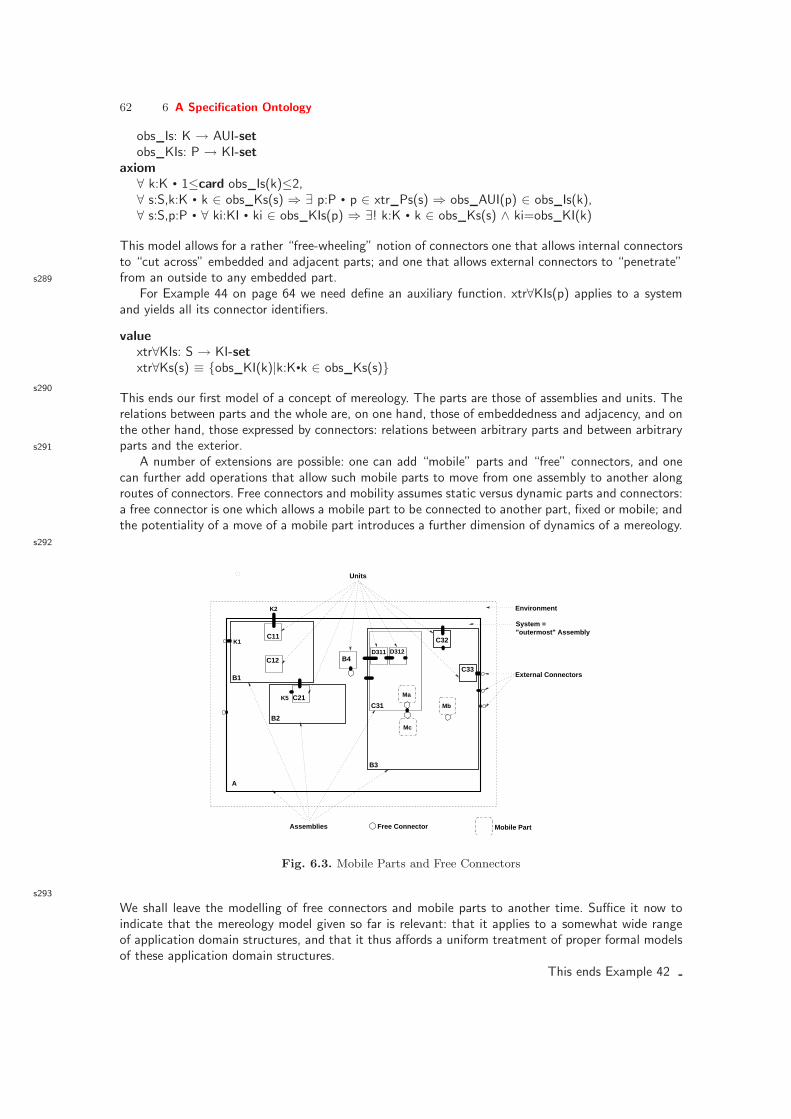
62 6 A Specification Ontology
obs Is: K → AUI-setobs KIs: P → KI-set
axiom∀ k:K • 1≤card obs Is(k)≤2,∀ s:S,k:K • k ∈ obs Ks(s) ⇒ ∃ p:P • p ∈ xtr Ps(s) ⇒ obs AUI(p) ∈ obs Is(k),∀ s:S,p:P • ∀ ki:KI • ki ∈ obs KIs(p) ⇒ ∃! k:K • k ∈ obs Ks(s) ∧ ki=obs KI(k)
This model allows for a rather “free-wheeling” notion of connectors one that allows internal connectorsto “cut across” embedded and adjacent parts; and one that allows external connectors to “penetrate”from an outside to any embedded part.s289
For Example 44 on page 64 we need define an auxiliary function. xtr∀KIs(p) applies to a systemand yields all its connector identifiers.
valuextr∀KIs: S → KI-setxtr∀Ks(s) ≡ obs KI(k)|k:K•k ∈ obs Ks(s)
s290This ends our first model of a concept of mereology. The parts are those of assemblies and units. Therelations between parts and the whole are, on one hand, those of embeddedness and adjacency, and onthe other hand, those expressed by connectors: relations between arbitrary parts and between arbitraryparts and the exterior.s291
A number of extensions are possible: one can add “mobile” parts and “free” connectors, and onecan further add operations that allow such mobile parts to move from one assembly to another alongroutes of connectors. Free connectors and mobility assumes static versus dynamic parts and connectors:a free connector is one which allows a mobile part to be connected to another part, fixed or mobile; andthe potentiality of a move of a mobile part introduces a further dimension of dynamics of a mereology.
s292
Environment
System =
A
D311 D312
C31
B3
C12
B1
Units
Assemblies
B4
C11
C21
C32"outermost" Assembly
External Connectors
K2
B2
K5 Ma
Mc
Mb
Mobile PartFree Connector
C33
K1
Fig. 6.3. Mobile Parts and Free Connectors
s293
We shall leave the modelling of free connectors and mobile parts to another time. Suffice it now toindicate that the mereology model given so far is relevant: that it applies to a somewhat wide rangeof application domain structures, and that it thus affords a uniform treatment of proper formal modelsof these application domain structures.
This ends Example 42

6.3 Simple Entities and Behaviours 63
s294
Summarising we find, for discrete simple entities, that atomic entities are characterisable by theirattributes (as well as by the operations that apply to entity arguments); and that compositeentities are characterisable by their attributes, the sub-entities from which they are made up andthe mereology, i.e., the part-whole relations between these sub-entities (as well as by the operationsthat apply to entity arguments). Continuous entities we treat almost as we treat atomic entitiesexcept that we can speak of, i.e., define, functions that decompose a continuous entity of kindC into an arbitrary number of continuous entities of the same kind C, and vice-versa: compose acontinuous entity of kind C from an arbitrary number of continuous entities of the same kind C.
6.3.2 Behaviours s295
Behaviours can be simple, sequential, and behaviours can be highly composite. To define be-haviours we need notions of states and actions: By a domain state we mean any collection of simpleentities — so designated by the domain engineer. By a domain action we mean the invocation ofan operation which “changes” the state.6 s296
Definition 39 – Behaviours: (i) By a behaviour we shall understand either a simple, sequentialbehaviour, or a simple parallel (or concurrent) behaviour, or a communicating behaviour. (ii) Bya simple, sequential behaviour we shall understand a sequence of actions and events (the latterto be defined shortly). (iii) By a simple parallel (or concurrent) behaviour we shall understand aset of simple, sequential behaviours. (iv) By a communicating behaviour we shall understand a setof simple parallel behaviours which in addition (to being simple parallel behaviours) communicatemessages between one-another.
s297
We shall base our formal specification of behaviours on the use of CSP (Hoare’s CommunicatingSequential Processes [81,82,130,134]). Other concurrency formalisms can, of course, be used: Petrinets [91,115,123–125], Message Sequence Charts (MSCs) [86–88], Statecharts [71–74,76], or other.
Communication, between two behaviours (CSP processes), P and Q is in CSP expressed by theCSP output and input clauses: ch ! e, respectively ch ? where ch designates a CSP channel. s298
typeA, B, M
channelch:M
valueav:A, bv:BS = P(av) ‖ Q(bv)P: A → out ch UnitP(a) ≡ ... ch!E(a) ... P(a′)Q: B → in ch UnitQ(b) ≡ ... let v = ch? in ... Q(b′) end
P Q
ch ?
V
ch ! E(a)s299
where a, a′ and b, b′ designate process P, respectively process Q state values provided to processinvocations (with a′ and b′ resulting from “calculations” not shown in the bodies of the definitionsof P and Q. av and bv are initial entities. S is the overall system behaviour of two communicatingbehaviours operating in parallel (‖). M designates the type of the messages sent over channel ch.
We shall now show a duality between entities and behaviours. The background for this dualityis the following: In everyday parlance we speak of some domain phenomena both as being entitiesand as embodying behaviours. s300
Example 43 – Entities and Behaviours: A train is the composite entity of one or more engines(i.e., locomotives) and one or more passenger and/or freight cars.
6Since we shall be expressing our formalisations in a pure, functional language, state changes areexpressed by functions whose signature include state entity types both as arguments and as results.

64 6 A Specification Ontology
typeTrain, Engine, PassCar, FreightCarCar = PassCar|FreightCar
valueobs Engine: Train → Engineobs Carl: Train → Car∗
axiom∀ tr:Train • card obs Carl(tr)>0
s301A train is also the behaviour whose state include the time dependent train location and the states ofthese engines and cars and whose sequence of actions comprise the arrival and stop of the train atstations, the unloading and loading of passengers and freight at stations, the start-up and departureof trains from stations and the continuous movement, initially at accelerated speeds, then constantspeed, finally at decelerating speeds along the rail track between stations — occasionally allowing forstops at track segment blocking signals. A train behaviour event could be that a cow presence of thetrack causes interrupt of scheduled train behaviour. Et cetera.s302
typeT, Loc,TrainBehaviour = T →m Train
channelnet channel (is at station|Bool)
valueobs Loc: Train → Loctrain: Train → T → out,in net channel → Unittrain(tr)(t) ≡
if is at Station(obs Loc(tr))then
let (tr′,t′) = stop train(tr)(t);let (tr′′,t′′) = load unload passengers and freight(tr′)(t′) inlet (tr′′′,t′′′) = move train(tr′′)(t′′) in
[ assert: ∼is at Station(obs Loc(tr′′′)) ]train(eσ′′,(el′,pfl′),loc′)(t′) end end end
elselet (tr′,t′) = move train(tr)(t) in train(tr′)(t′) end
ends303
Here we leave undefined a number of auxiliary functions:
valueis at Station: Loc → out,in net channel Boolstop train: Train → T → Train × Tload unload passengers and freight: Train → T → Train × Tmove train: Train → T → Train × T
The above “model” of a train behaviour is really not of the kind (of models) that we shall eventuallyseek. The predicate is at Station communicates with the net behaviour (not shown). The functionload unload passengers and freight communicates with the net behaviour (platforms, marshallingyards, etc., not shown). It is a rough sketch meant only to illustrate the process behaviour.
s304
Example 42 illustrated a very general class of mereologies. The next example, Example 44 willshow how the duality between entities and behaviours can be “drawn” to an ultimate conclusion !
s305
Example 44 – Mereology: Parts and Wholes (2): The model of mereology presented in Exam-ple 42 on page 60 (Pages 60–62) focused on the following simple entities

6.3 Simple Entities and Behaviours 65
• the assemblies,• the units and• the connectors.
To assemblies and units we associate CSP processes, and to connectors we associate CSP channels,one-by-one [81, 82, 130,134]. s306
The connectors form the mereological attributes of the model.To each connection we associate a CSP channel, it is “anchored” in two parts: if a part is a unit then
in “its corresponding” unit process, and if a part is an assembly then in “its corresponding” assemblyprocess.
From a system assembly we can extract all connector identifiers. They become indexes into an arrayof channels. Each of the connector channel identifiers is mentioned in exactly one unit or one assemblyprocess. s307
From a system which is an assembly, we can extract all the connector identifiers as well as allthe internal connector identifiers. They become indexes into an array of channels. Each of the externalconnector channels is mentioned in exactly one unit or one assembly process; and each of these internalconnection channels is a mentioned in exactly two unit or assembly processes. The xtr∀KIs(s) belowwas defined in Example 42 (Page 62). s308
values:Skis:KI-set = xtr∀KIs(s)
typeChMap = AUI →m KI-set
valuecm:ChMap = [ obs AUI(p)7→obs KIs(p)|p:P•p ∈ xtr Ps(s) ]
channelch[ i|i:KI•i ∈ kis ] MSG
valuesystem: S → Processsystem(s) ≡ assembly(s)
s309
valueassembly: a:A→in,out ch[ cm(i) ]|i:KI•i ∈ cm(obs AUI(a)) processassembly(a) ≡MA(a)(obs AΣ(a)) ‖‖ assembly(a′)|a′:A•a′ ∈ obs Ps(a) ‖‖ unit(u)|u:U•u ∈ obs Ps(a)
obs AΣ: A → AΣ
MA: a:A→AΣ→in,out ch[ cm(i) ]|i:KI•i ∈ cm(obs AUI(a)) processMA(a)(aσ) ≡ MA(a)(AF(a)(aσ))
AF : a:A → AΣ → in,out ch[ em(i) ]|i:KI•i ∈ cm(obs AUI(a))×AΣ
s310The unit process is defined in terms of the recursive meaning function MU function which requiresaccess to all the same channels as the unit process.
valueunit: u:U → in,out ch[ cm(i) ]|i:KI•i ∈ cm(obs UI(u)) processunit(u) ≡ MU (u)(obs UΣ(u))obs UΣ: U → UΣ
MU : u:U → UΣ → in,out ch[ cm(i) ]|i:KI•i ∈ cm(obs UI(u)) process

66 6 A Specification Ontology
MU (u)(uσ) ≡ MU(u)(UF(u)(uσ))
UF : U → UΣ → in,out ch[ em(i) ]|i:KI • i ∈ cm(obs AUI(u)) UΣ
s311The meaning processesMU andMA are generic. Their sole purpose is to provide a never ending recur-sions. “In-between” they “makes use” of assembly, respectively unit specific functions here symbolisedby AF and UF .s312
The assembly function “first” “functions” as a compiler. The ‘compiler’ translates an assemblystructure into three process expressions: the MA(a)(aσ, aρ) invocation, the parallel composition ofassembly processes, a′, one for each sub-assembly of a, and the parallel composition of unit processes,one for each unit of assembly a — with these three process expressions “being put in parallel”. Therecursion in assembly ends when a sub-. . . -assembly consists of no sub-sub-. . . -assemblies. Then thecompiling task ends and the many generatedMA(a)(aσ, aρ) andMU(u)(uσ, uρ) process expressionsare invoked.s313
We can refine the meaning of connectors. Each connector, so far, was modelled by a CSP channel.CSP channels serve both as a synchronisation and as a communication medium. We now suggest tomodel it by a process. A channel process can be thought of as having four channels and a bufferingprocess. Connector, κ:K, may connect parts πi, πj . The four channels could be thought of as indexedby (κ, πi), (πi, κ), (κ, πj) and (πj , κ). The process buffer could, depending on parts pi, pj , be eitherqueues, sets, bags, stacks, or other. This ends Example 44
s314
The duality between simple entities and behaviours has the attributes of atomic as well as ofcomposite entities become the state in which the entity behaviours evolve.
Whereas — in principle — the mereology of how sub-entities compose into entities are modelledas in Example 42, namely in terms of sorts, observer functions and axioms over unique identifiersof simple entities, their attributes are usually modelled in a more model-oriented way, in terms ofmathematical sets, Cartesians, sequences and maps.
6.4 Functions and Events s315
We shall consider events to be special cases of function invocations.
6.4.1 Functions
Definition 40 – Function: By a function we shall understand something (a functional entity)which when applied to an entity, which we shall call an argument of the function, yields a resultwhich is also an entity.
We shall refer to the application of a function to an argument as an invocation. Functions arecharacterised by the function signature or just signature and by their function definition. We showa number of function (and process) signatures:s316
typeA, B, M1, M2
channelchi:MI, cho:MO
The above type definitions and channel declarations are used below:
valuef0: A → Bf1: Unit → Bf2: Unit → Unitf3: A → Unitf4: A → in chi B
f5: A → in chi out cho Bf6: A → out cho Bf7: A → in chi Unitf8: A → in chi out cho Unitf9: A → out cho Unit

6.4 Functions and Events 67
In Example 44 we used the literal process where we now, and in future, shall use the more properRSL term Unit. The reason for using process in the example was that the term ‘unit’ was used toname a sort of simple entities. s317
• f0 designates a (“pure, applicative”) function from A into B.• f1 designates a constant function: takes no argument, i.e., invocation is expressed by f1(), but
yields a (constant) value in B.• f2 designates a process (i.e., a process function, one that never terminates). Invocation is
expressed by f2(),• f3 designates a process, accepting arguments in A and otherwise never terminating.• f4 designates a function, accepting arguments in A and inputs, of type MI, on channel chi and
otherwise terminating yielding a value of type B.• f5 designates a function, accepting arguments in A, and inputs, of type MI, on channel chi,
offers outputs, of type MO, on channel cho, and otherwise terminating yielding a value of typeB. s318
• f6 designates a function, accepting arguments in A, offers outputs, of type MO, on channel cho,and otherwise terminating yielding a value of type B.
• f7 designates a function, accepting arguments in A, and inputs, of type MI, on channel chi andotherwise never terminating.
• f8 f7 designates a function, accepting arguments in A, inputs, of type MI, on channel chi, offersoutputs, of type MO, on channel cho, and otherwise never terminating.
• f9 designates a function, accepting arguments in A, offers outputs, of type MO, on channel cho,and otherwise never terminating.
s319
For functions f4–f9 you may replace A by Unit to obtain further signatures. Thus the literal Unit,to the left of the→ designates that no input is to be provided, and to the right of the→ designatesa never ending process. s320
We show a number of function signatures exemplifying “Currying”:
typeA, B, C, D
valuef′: A × B × C → Df′′: A × B → C → Df′′′: A → B → C → D
invocation examples:f′(a,b,c)f′′(a,b)(c)f′′′(a)(b)(c)
s321
We show two forms of function definitions:
typeA, B
value
f: A∼→ B
f(a) as bpre P(a)post Q(a,b)
typeA, B
value
g: A → B [ A∼→ B ]
g(a) ≡ E(a)[ pre P(a) ]
s322
f is defined by a pair of pre/post conditions expressed by the predicates P(a) and Q(a,b) re-spectively. The clause ‘as b’ expresses that the result is named b g and allows Q to refer to theresult.
g is defined by an explicit (“abstract algorithmic”) expression E(a). To avoid cluttering E(a)with basically a test on P(a) (should g not be total on A, that test is brought as a pre condition.

68 6 A Specification Ontology
6.4.2 Events s323
Definition 41 – Event: By an event we shall generally understand a state change that satisfiesa given predicate:
typeΣ
valueeventi: Σ × Σ → Bool
Given two states: σ, σ′, if eventi(σ,σ′) holds then we say that event eventi has occurred.s324
This definition of an event is much too general. Of course, the domain (or requirements or softwaredesign) engineer is the one who decides which events to describe. But we shall accept it on formalgrounds. More pragmatically we shall introduces the notions of internal event and external event.Most actions cause events — and they are all internal events. And most of these internal eventsare (usually) “uninteresting”.s325
A few internal events are interesting, that is, cause state changes “over-and-above” thoseprimarily intended by the action.
Example 45 – Interesting Internal Events: Examples of what we would term interesting internalevents are: Banking: A bank changes its interest rates; Train Traffic: a train is cancelled, etc.; OilPipeline: a pipeline runs dry of oil (due, for example, to valve and pump settings); and Health Care: apatient is give a wrong medicine (a form of medical malpractice).
s326
External events are events cause by “functions” beyond “our” control. That is, we postulate thatsome, maybe we could call it “demonic” function caused an event.
Example 46 – External Events: Examples of external events are: Banking: a major debitor defaultson a loan; Train Traffic: a train runes off the tracks; Oil Pipeline: a pipeline bursts; and Health Care:a patient dies.
s327
Internal events are typically modelled by providing the usual function, that is, action definitionswith a suitable case distinction based on the eventi predicate.
valuefunction: A → Σ → Σ × Bfunction(a)(σ) ≡
let (σ′,b) = action(a)(σ) inif eventi(σ,σ′)
then cope with internal event(a)(σ,σ′)else (σ′,b) end end
action: A → Σ → Σ × Bcope with internal event: A → (Σ×Σ) → Σ × B
s328We may model external events as inputs on channels that can thus be said to “originate” in theenvironments — but for which functions definitions set aside an alternative choice of acceptingsuch inputs from the environment.
typeA, B, Σ, Event
channelx ch:Event
valuefunction: A → Σ → in x ch Σ Bfunction(a)(σ) ≡
action(a)(σ)

6.5 On Descriptions 69
⌈⌉let event = x ch ? in cope with external event(a)(event)(σ) end
action: A → Σ → Σ × Bcope with external event: A → Event → Σ → Σ × B
6.5 On Descriptions s329
We refer to the subsections of Sect. 2.1, Pages 5–7.The discussion of this section amounts to establishing a meta-theory of domains, that is, a
theory of the abstract, conceptual laws of describing domains in contrast to a theory of any onespecific domain, that is, a theory of the concrete, physical and human laws of the described domain.
In our discussion we will rely on understanding specifically referenced examples. This under-standing might very well be improved as a result of understanding the message of this section.
6.5.1 What Is It that We Describe ? s330
What is it that our descriptions denote ?7 The answer is: the “things” that the nouns of ourdescription “points to” are the actual things, “out there”, in the domain. The denoted individualsare not “figs of our imagination”8. They are ‘real’, ‘actual’, can be pointed to, seen, heard, touched,smelled, or otherwise measured by physical, including chemical/physical apparatus(es) !
Therefore there can be no “identical” copies. If two sensed or measured phenomena are “equal”then they are the same phenomenon.
6.5.2 Phenomena Identification s331
We have in various examples, as from Example 10 on page 9 introduced the abstract conceptof unique identifiers: of hubs and links (Example 10 on page 9), of parts (assemblies and units)(Example 42 on page 60), and in many later examples. These unique identifications are, in a sense,a mere technicality. We need the unique identifications when we wish to express mereologicalproperties such a “part of”, “next to”, “connected to”, etcetera. Therefore, if two sensed or s332
measured and described phenomena are “equal”, except for their postulated unique identification,then they are still the same phenomenon, and there is a problem of description. We next turn tosuch ’problems of description’.
6.5.3 Problems of Description s333
We can illustrate a number of ‘problems of description’. (i) Unique identifications: two (or more)hubs that are claimed to have distinct hub identifiers, cf. Example 10 on page 9, but otherwisehave identical values for all conceivable attributes, including spatial location must be the samehub, i.e., have identical hub identifier; (ii) Observability: if from a hub, cf. Example 10 on page 9,we can observe a link, hence all its connected links, and, vice versa, from a link we can observeits connected hubs, and not merely their identifiers, but the ‘real’ phenomena, then we can arguethat we can observe, from any hub the entire net: all hubs and all links, and that is counter to ourintuition, we claim, of how we observe.
7This question is just another way of expressing the question of the title of this subsection (i.e.,Sect. 6.5.1).
8I apologize to more philosophically inclined readers: ours is not a discourse on ontology in the philo-sophical sense: What may exists ? etcetera. Our setting is computing science and software engineering— so we have no qualms about postulating that what I can sense, every person in full control of all hersenses can sense and in an identical way !
70 6 A Specification Ontology
6.5.4 Observability s334
That is: we reject the dogma: “The Universe in a Single Atom”9, that is, that all can be observedfrom a single “position”.
But this rejection begs the issue “What Do We Mean by Observability ?”In the following we shall treat observability of simple entities and their attributes on par, that
is, not make a distinction. Later we shall make a distinction between observing simple entities andobserving attributes.
Simple Observability s335
The simple part of an answer to this question, and, mind you, it is an answer that is based onour computing science and software engineering viewpoint, concerns that which can be physicallyobserved of any domain phenomenon “itself”, that is, of the phenomenon observed in isolation.That part of the answer goes like this: of a physically manifested phenomenon we can observe allthat can be physically sensed: seen, heard, smelled, tasted, and touched; as well as measured byphysical/chemical apparatus(es).
Not-so-Simple, Simple Entity Observability s336
The not-so-simple part of an answer focuses on simple entities and concerns that which can bephysically observed of the “immediate” mereology of the simple entity “itself”, that is, of theparts to which that simple entity is connected. Here the answer is: One can observe immediates337
phenomenological and conceptual connections, that is, the simple entity parts that are connectedto the entity under review, and by reference to their identity — hence the need for the identityconcept; and similarly for operations, event and behaviours: which operations directly invoke otheroperations, directly cause events, and, in general, directly participate in behaviours; which events“trigger” operations, other events, and, in general, directly participate in behaviours; and whichbehaviours synchronise and/or communicate with other behaviours.
6.5.5 On Denoting s338
Yes, we do know that Bertrand Russel wrote a famous paper with this title [131]. But our in-tention here is less ‘lofty’, and, perhaps not ! When, above, we write: the denoted individualsare not “figs of our imagination” and they are ‘real’, ‘actual’, can be pointed to, seen, heard,touched, smelled, or otherwise measured by physical, including chemical/physical apparatus(es),then it is our intention that we express. We can make that claim as far as the informal narrativedescription is concerned. But when our description is formalised, then what ? Our formal descrip-tion language has a semantics. That semantics ascribes to our formalisation some mathematicalvalues, structures. That is, our narrative is of the ‘real thing’, and our formalisation is a model ofthe real thing. So there are two notions of ‘denoting’ at play here. an informal one: the relations339
between the narrative description and the physical (incl. human) phenomena and a formal one:the relation between the syntax of our formal description and its semantics, i.e., ‘the model’. Thetwo notions relate, but only informally: enumerated lines of the narrative has been “syntactically”,that is informally, related to “identically” numbered formula lines, with the informal claim that anumbered narrative line “means” the same as the same-numbered formula line !
9Also the title of a book by HH The 14thDalai Lama: ‘The Universe in a Single Atom’: Reason andFaith

6.5 On Descriptions 71
6.5.6 A Dichotomy s340
Example 42 (Pages 60–63), we now claim, has the narrative denote classes of real phenomena andhas the formalisation model the syntax and syntactic well-formedness of a large class of such realphenomena. Later, in Example 44, (Pages 64–66), we now claim, has the (the same) narrative (asin Example 42) indicate conceptual semantic models of with the formalisation explicitly designat-ing classes of such semantics models. So the transition between the two examples, Example 42 s341
and Example 44, signal a reasonably profound “shift” from (informally) designating actual phe-nomena and (formally) denoting their algebraic structures, to, informally and formally, referringto semantic models in terms of behaviours and states. There is no dichotomy here, just a shift ofabstraction.
6.5.7 Suppression of Unique Identification s342
When comparing, for example, two simple entities one is comparing not only their attributes butalso, when the entities are composite, their sub-entities. Concerning unique identifiers of simpleentities we have this to say: We can decide to either include unique identifiers as an entity attribute,or we can decide that such identifiers form a third kind of observable property of a simple entitythe two others being (“other”) attributes — as we see fit to define and the possible sub-entities ofcomposite entities. Either way, we need to introduce a meta-linguistic operator10, say s343
SI : Simple observable entity value → Anonymous simple entity value
The concept of an anonymous value is also meta-linguistic. The anonymous value is basically “thesame, i.e., “identical” value as is the simple entity value (from which, through SI
11, it derives) withthe single exception that the simple entity value “possesses” the unique identifier of the observableentity value and the anonymous entity value does not.
6.5.8 Laws of Domain Descriptions s344
Preliminaries
When we wish to distinguish one simple entity phenomenon from another then we say that thetwo (“the one and the other”) are distinct. To be distinct to us means that the two phenomenahave distinct, that is, unique identifiers. Being simple entity phenomena, separately observablein the domain, means that their spatial (positional) properties are distinct. That is their anony-mous values are distinct. Meta-linguistically, that is, going outside the RSL framework12, we can“formalise” this: s345
typeA [ A models a type of simple entity phenomena ]I13 [ I models the type of unique A identifiers ]
valueobs I: A → I
axiom∀ a,a′:A • obs I(a)6=obs I(a′) ⇒ SI(a)6=SI(a
′)
s346
10The operator SI is meta-linguistic with respect to RSL: it is not part of RSL, but applies to RSL values.11The S stands for “suppress” and the I for the suppressed unique identifier.12but staying within a proper mathematical framework — once we have understood the mathematical
properties of SI and proper RSL values and ‘anonymous’ values (which, by the way, are also RSL values)13We have here emphasized I , the type name of the type of unique A identifiers. Elsewhere in this book
we treat types of unique identifiers of different types of observable simple entities as “ordinary” RSL types.Perhaps we should have “singled” such unique identifier type names out with a special font ? Well, we’llleave it as is !

72 6 A Specification Ontology
The above applies to any kind of observable simple entity phenomenon A. It does not necessarilyapply to simple entity concepts.
Example: Two uniquely identified timetables may have their anonymous values be the exactsame value. 2s347
Simple entity phenomena, in our ontology, are closely tied to space/time “co-ordinates” —with no two simple entity phenomena sharing overlapping space. Concepts are, in our ontology,not so constrained, that is, we allow “copies” although uniquely named ! That is, two seeminglydistinct concepts may be the same when “stripped” of their unique names !
Some Domain Description Laws s348
We shall just bring a few domain description laws here. Enough, we hope, to spur further researchinto ‘laws of description’.s349
Domain Description Law 1 – Unique Identifiers: If two observable simple entities have the sameunique identifier then they are the same simple entity.
Any domain description must satisfy this law. The domain describer must, typically throughaxioms, secure that the domain description satisfy this law. Thus there is a proof obligation to bedispensed, namely that the unique identifier law holds of a domain description.s350
Domain Description Law 2 – Unique Phenomena: If two observable simple entities have differentunique identifiers then their values, “stripped” of their unique identifiers are different.
Any domain description must satisfy this law. The domain describer must, typically throughaxioms, secure that the domain description satisfy this law. Thus there is a proof obligation to bedispensed, namely that the unique phenomena law holds of a domain description.s351
Domain Description Law 3 – Space Phenomena Consistency: Two otherwise unique, and hencedistinctly observable phenomena can, spatially, not overlap.
s352
We can express the Space/Time Phenomena Consistency Law meta-linguistically, yet in a propermathematical manner:
typeE [ E is the type name of a class of observable simple entity phenomena ]I [ I is the type name of unique E identifiers ]L [ L is the type name of E locations ]
valueobs I: E → Iobs L: E → L
axiom∀ e,e′:E • obs I(e)6=obs I(e′) ⇒ obs L(e) ⊓ obs L(e′) = ∅
We can assume that this law always holds for otherwise unique, and hence distinctly observablephenomena.s353
Domain Description Law 4 – Space/Time Phenomena Consistency: If a simple entity (that hasthe location property), at time t is at location ℓ, and at time t′ (larger than t) is at location ℓ′ (differentfrom ℓ), then it moves monotonically from ℓ to ℓ′ during the interval (t, t′).
Specialisations of this law are, for example, that if the movement is of two simple entities, liketwo trains, along a single rail track and in the same direction, then where train si is in front oftrain sj at time t, train sj cannot be in front of train si at time t′ (where t′− t is some small timeinterval).

6.6 Exercises 73
Discussion s354
There are more domain description laws. And there are most likely laws that have yet to be“discovered” ! Any set of laws must be proven consistent. And any domain description must beproven to adhere to these (and “the” other) laws. We decided to bring this selection of laws becausethey are a part of the emerging ‘domain science’. Laws 3 on the preceding page and 4 on the facingpage are also mentioned, in some other form, in [132].
Are these domain description laws laws of the domain or of their descriptions, that is, are theydomain laws ? We leave the reader to ponder on this !
6.6 Exercises
See Items 7–10 (of Appendix D, starting Page 230).


Part IV
Domains


7
Domain Engineering
s355 acm-tsode-1
7.1 The Core Stages of Domain Engineering
The core stages of domain engineering are those of modelling the following domain facets: intrinsics(Sect. 7.3), support technologies (Sect. 7.4), management and organisation (Sect. 7.5),rules andregulations (Sect. 7.6), scripts (contracts and licenses) (Sect. 7.7) and human behaviour (Sect. 7.8)of the domain. s356
An important stage of domain engineering is that of rough sketching the business processes.This stage is “sandwiched” in-between the opening stages of domain acquisition and domainanalysis. s357
The decomposition of these core stages into exactly these facet description stages is one ofpragmatics. Experience has shown that this decomposition into modelling stages leads to a suitablebase for a final model. That is, the domain engineers may follow, more-or-less strictly the facetstage sequence hinted at above but the domain engineers may, very well, in the end, present thefinal domain description without clear delineations, in the description, between these facets. Inother words, the decomposition and the principles of each individual facet stage, we think, providesa good set of guidelines for the domain engineers on how to proceed. s358
These core stages are preceded by a number of opening stages and succeeded by a number ofclosing stages.
The opening and closing stages, cf. Sects. 7.9.1 on page 128 and 7.9.2 on page 128, except forthe business process sketching stage, are here considered less germane to the proper understandingof the domain concept.
7.2 Business Processes s359
The rough-sketching of business processes shall serve as an “easiest”, informal way of starting themore systematic domain acquisition process.
Definition 42 – Business Process: By a business process we understand the procedurally de-scribable aspects, of one or more of the ways in which a business, an enterprise, a factory, etc.,conducts its yearly, quarterly, monthly, weekly and daily processes, that is, regularly occurringchores. The business processes may include strategic, tactical and operational management and s360
work-flow planning and decision activities; and the administrative, and where applicable, the mar-keting, the research and development, the production planning and execution, the sales and theservice (work-flow) activities — to name some.

78 7 Domain Engineering
7.2.1 General Remarks s361
A domain is often known to its stakeholders by the various actions they play in that domain. Thatis, the domain is known by the various sequences of entities, functions and events the stakeholdersare exposed to, are performing and are influenced by. Such sequences are what we shall hereunderstand as business processes.s362
In our ongoing example, that of railway systems, informal examples of business processes are:for a potential passenger to plan, buy tickets for, and undergo a journey. For the driver of thelocomotive the sequence of undergoing a briefing of the train journey plan, taking possession ofthe train, checking some basic properties of that train, negotiating its start, driving it down theline, obeying signals and the plan, and, finally entering the next station, stopping at a platform,and concluding a trip of the train journey — all that constitutes a business process. For a traindispatcher, the monitoring and control of trains and signals during a work shift constitutes abusiness process.s363
Describing domain intrinsics focuses on the very essentials of a domain. It can sometimes be abit hard for a domain engineer, in collaboration with stakeholders, to decide which are the domainintrinsics. It can often help (the process of identifying the domain intrinsics) if one alternatively, orhand in hand analyses and describes what is known as the business processes. From a descriptionof business processes one can then analyse which parts of such a description designate, i.e., areabout or relate to, which facets.
7.2.2 Rough Sketching s364
Initially the domain engineer proceeds by sketching. We use the term rough sketching1 to em-phasise that a rough sketch is just a preparatory document. A roughly sketched business processappears easier to make, that is, gets one started more easily. A rough sketch business process doesnot have to conform to specific principles about what to describe first, whether to first describephenomena or concepts; whether to first describe discrete facts or continuous; whether to firstdescribe atomic facts or composite; whether to first describe informally or formally; etcetera.s365
Principle 1 – Describing Domain Business Process Facets: As part of understanding any (atleast human-made) domain it is important to delineate and describe its business processes. Initiallythat should preferably be done in the form of rough sketches. These rough sketches should —again initially — focus on identifiable simple entities, functions, events and behaviours. Naturally,being business processes, identification of behaviours comes first. Then be prepared to rework thesedescriptions as the modelling of domain facets starts in earnest.
s366
Roughly sketched business processes help the domain engineer in the more general domain acqui-sition effort. Domain stakeholders can be asked to sketch the business processes they are part of.The domain engineer, interacting with the domain stakeholder can clarify open points about asketched business process. And the domain engineer can elicit facts about the domain as inspiredby someone else’s sketch.
7.2.3 Examples (I) s367
Example 47 – A Business Plan Business Process: The board of any company instructs its chiefexecutive officer (CEO) to formulate revised business plans.2 Briefly, a business plan is a plan for howthe company — strategically, tactically and, to some extent, operationally — wishes to conduct itsbusiness: what it strives for, product-wise, image-wise, market-share-wise, financially, etc. The CEOdevelops a business plan in consultation with executive layers of (i.e., with strategic) management.Strategic management (in-between) discusses the plan (which the CEO wishes to submit to the Board)with tactical management, etc. Once generally agreed upon, the CEO submits the plan to the Board.
s368
1To both say ‘rough’ and ‘sketching’ may, perhaps be saying the same thing twice: sketches usuallyare rough.
2A business plan is not the same as a description of the business’ processes.

7.2 Business Processes 79
Example 48 – A Purchase Regulation Business Process: In our “example company”, purchase ofequipment must adhere to the following — roughly sketched — process: Once the need for acquisitionof one or more units of a certain equipment, or a related set of equipment, has been identified, the staffmost relevant to take responsibility for the use of this equipment issues a purchase inquiry request. Thepurchase inquiry request is sent to the purchasing department. The purchasing department investigatesthe market and reports back to the person who issued the request with a purchase inquiry reportcontaining facts about zero, one or more possible equipment choices, their prices, and their purchase(i.e., payment), delivery, service and guarantee conditions. The person who issued the purchase inquiry s369
request may now proceed to issue a purchase request order, attach the purchase inquiry report andsend this to the relevant budget controlling manager for acceptance. If purchase is approved then thepurchasing department is instructed to issue, to the chosen supplier, a purchase request order. Oncethe supplier delivers the ordered equipment, the purchasing department inspects the delivery and issuesan equipment inspection report. An invoice from the supplier for the above-mentioned equipment isonly paid if the equipment inspection report recommends to do so. Otherwise the delivered equipmentis returned to the supplier.
s370
Example 49 – A Comprehensive Set of Administrative Business Processes: The Universityof California at Irvine (UCI), had their Administrative and Business Services department suggest, as alearning example, the description of a number of business processes. The “learning” had to do, actually,with business process re-engineering (BPR). So we really should bring the below example into Sect. 8.5!We quote from their home Web page [142]: s371
1. Human Resources: “Examine the hiring business process of the University, including the applicantprocess. Special emphasis should be given to simplifying the process, identifying those parts wherethere is no value added — i.e., where those parts of the process which one considers simplifying“away” add no value. Increase speed of response to applicant and units, and reduce process costswhile achieving high quality.” s372
2. Renovation: “Review the campus’ remodelling and alterations business process, and develop rec-ommendations to improve Facilities Management services to UCI departments for small projects(under $50,000) and minor capital projects (up to $250,000). Special emphasis should be givento simplifying the process; identifying those parts where there is no value added to the customer’sproduct; to increase speed and flexibility of response; and to reduce process costs while achievinghigh quality.” s373
3. Procurement: “Review the campus procurement business process and develop recommendations/-solutions for process improvement. The redesigned process should provide “hassle-free” purchasing,give a quick response time to the purchaser, be economical in terms of all costs, be reasonablyerror-free and be compliant with (US) Federal procurement standards.” s374
4. Travel: “Study the travel business process from the stage when a staff member identifies the needto travel to the time when reimbursement is received. Analyze and redesign the process through asix step program based on the following business process improvement (BPI) principles: (i) simplifythe process, (ii) identify those parts where there is no value added to the customer, increase (iii)speed and (iv) flexibility of response, (v) improve clarity for responsibilities and (vi) reduce processcosts while meeting customer expectations from travel services. The redesign should reflectcustomerneeds, service, economy of operation and be in compliance with applicable regulations.” s375
5. Accounts payable: “Redesign the accounts payable business process to meet the following func-tional objectives (in addition to BPI measures): Payment for goods and services must assure thatvendors receive remittance in a timely manner for all goods and services provided to the University.Significantly improve the operation’s ability to serve campus customers while maintaining financialsolvency and adequate internal controls.” s376
6. Parking: “Review how parking permits are sold to students, faculty and staff with the intent ofomitting unnecessary steps and redundant data collection. The redesigned process should achievea dramatic reduction in time spent by people standing in line to purchase a permit, and reduceadministrative time (and cost) in recording and tracking permit sales.”

80 7 Domain Engineering
Please observe that the above examples illustrate requests for possible business process re-engineering— but that they also give rough-sketch glimpses of underlying business processes.
7.2.4 Methodology s377
Definition 43 – Business Process Engineering: By business process engineering we understandthe identification of which business processes should be subject to precise description, describingthese and securing their general adoption (acceptance) in the business, and enacting these businessprocess descriptions
s378
Principle 2 – Business Processes: Human-made universes of discourse3 entail the conceptof business processes. The principle of business processes states that the description of businessprocesses is indispensable in any description of a human-made universe of discourse. The principleof business processes also states that describing these is not sufficient: all facets must be described
s379
Principle 3 – Describing Domain Business Process Facets: As part of understanding any(at least human-made) domain it is important to delineate and describe its business processes.Initially that should preferably be done in the form of rough sketches. These rough sketches should— again initially — focus on identifiable entities, functions, events and behaviours. Naturally,being business processes, identification of behaviours comes first. Then be prepared to rework thesedescriptions as other facets are being described in depth
s380
Technique 1 – Business Processes: The basic technique of describing a human-made uni-verse of discourse involves: (i) identification and description of a suitably comprehensive set ofbehaviours: the behaviours of interest and the environment; (ii) identification and description, foreach behaviour, of the entities characteristic of this behaviour; (iii) identification and description,for each entity, of the functions that apply to entities, or from which entities are yielded; (iv)identification and description, for each behaviour, of the events that it shares — either with otherspecifically identified behaviours of interest, or with a further, abstract, environment
s381
Tool 1 – Business Processes: Further techniques and the basic tools for describing businessprocesses include: (1) RSL/CSP definition of processes, where one suitably defines their input/outputsignatures, associated channel names and types, and their process definition bodies;4 (2) Petris382
nets;5 (3) message and live sequence charts for the definition of interaction between behaviours;6
(4) statecharts for the definition of highly complex, typically interwoven behaviours;7 and (5) theusual, full complement of RSL’s type, function value, and axiom constructs and their abstracttechniques for modelling entities and functions
7.2.5 Examples (II) s383
We rough-sketch a number of examples. In each example we start, according to the principles andtechniques enunciated above, with identifying behaviours, events, and hence channels and the typeof entities communicated over channels, i.e. participating in events. Hence we shall emphasise, inthese examples, the behaviour, or process diagrams. We leave it to other examples to presentother aspects, so that their totality yields the principles, the techniques and the tools of domaindescription.s384
3Examples of human-made universes of discourse are: public administration, manufacturing industries(mechanical, chemical, medical, woodworking, etc.), transportation, the financial service industry (banks,insurance companies, securities instrument brokers, traders and exchanges, portfolio management, etc.),agriculture, fisheries, mining, etc.
4RSL/CSP [81,82,130,134] was covered in detail in Vol. 1, Chap. 21.5Petri Nets [91,115,123–125] were covered in detail in Vol. 2, Chap. 12.6Message [86–88] and live sequence charts [39,75,95] were covered in detail in Vol. 2, Chap. 13.7Statecharts [71–74,76] were covered in detail in Vol. 2, Chap. 14.
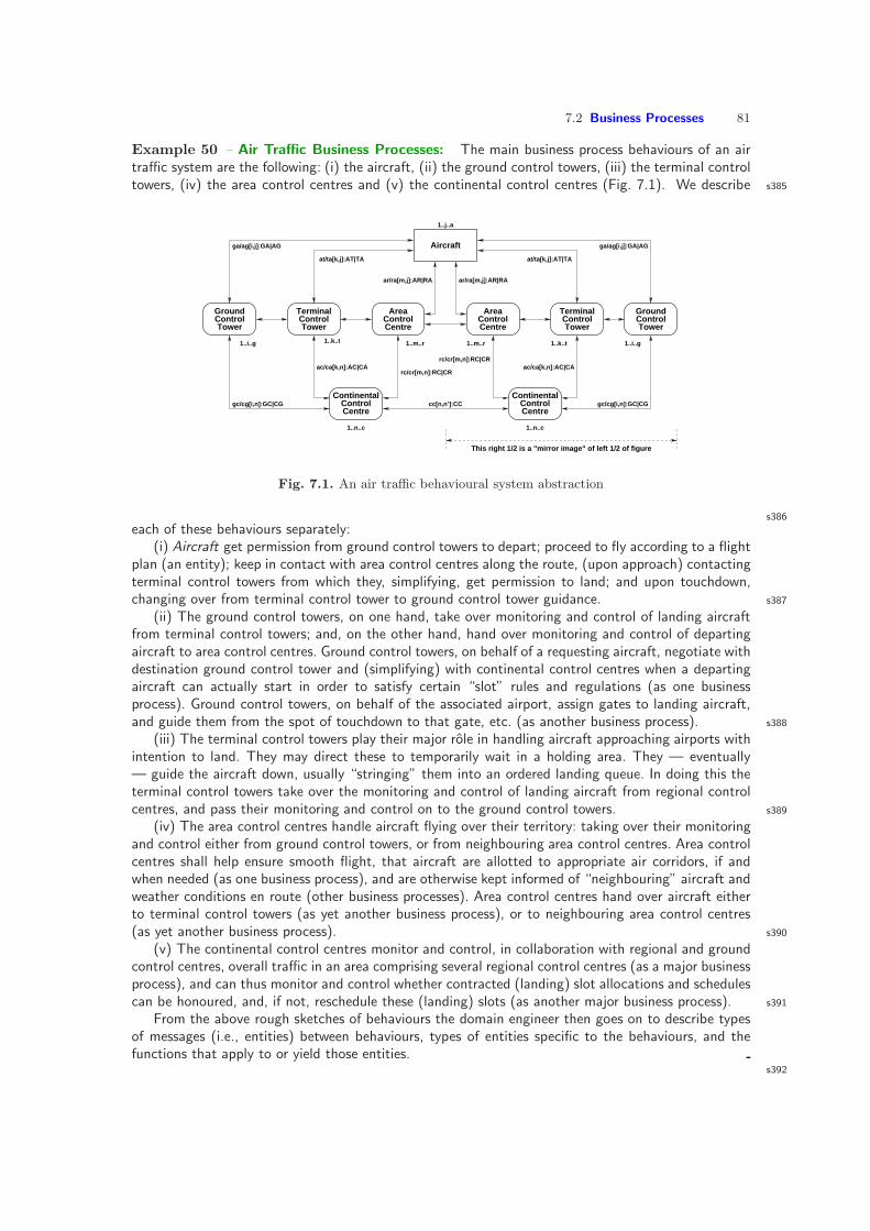
7.2 Business Processes 81
Example 50 – Air Traffic Business Processes: The main business process behaviours of an airtraffic system are the following: (i) the aircraft, (ii) the ground control towers, (iii) the terminal controltowers, (iv) the area control centres and (v) the continental control centres (Fig. 7.1). We describe s385
GroundControlTower
Aircraft
ControlTower
Continental
Control ControlControl
Control ControlContinental
TowerTower
GroundControl
1..k..t 1..m..r
1..n..c 1..n..c
1..j..a
1..i..g 1..m..r 1..k..t 1..i..g
This right 1/2 is a "mirror image" of left 1/2 of figure
ac/ca[k,n]:AC|CA
cc[n,n’]:CC
rc/cr[m,n]:RC|CRac/ca[k,n]:AC|CA
rc/cr[m,n]:RC|CR
ga/ag[i,j]:GA|AG ga/ag[i,j]:GA|AG
at/ta[k,j]:AT|TA at/ta[k,j]:AT|TA
gc/cg[i,n]:GC|CG
ar/ra[m,j]:AR|RA ar/ra[m,j]:AR|RA
gc/cg[i,n]:GC|CG
Terminal TerminalAreaArea
Centre Centre
CentreCentre
Fig. 7.1. An air traffic behavioural system abstraction
s386
each of these behaviours separately:(i) Aircraft get permission from ground control towers to depart; proceed to fly according to a flight
plan (an entity); keep in contact with area control centres along the route, (upon approach) contactingterminal control towers from which they, simplifying, get permission to land; and upon touchdown,changing over from terminal control tower to ground control tower guidance. s387
(ii) The ground control towers, on one hand, take over monitoring and control of landing aircraftfrom terminal control towers; and, on the other hand, hand over monitoring and control of departingaircraft to area control centres. Ground control towers, on behalf of a requesting aircraft, negotiate withdestination ground control tower and (simplifying) with continental control centres when a departingaircraft can actually start in order to satisfy certain “slot” rules and regulations (as one businessprocess). Ground control towers, on behalf of the associated airport, assign gates to landing aircraft,and guide them from the spot of touchdown to that gate, etc. (as another business process). s388
(iii) The terminal control towers play their major role in handling aircraft approaching airports withintention to land. They may direct these to temporarily wait in a holding area. They — eventually— guide the aircraft down, usually “stringing” them into an ordered landing queue. In doing this theterminal control towers take over the monitoring and control of landing aircraft from regional controlcentres, and pass their monitoring and control on to the ground control towers. s389
(iv) The area control centres handle aircraft flying over their territory: taking over their monitoringand control either from ground control towers, or from neighbouring area control centres. Area controlcentres shall help ensure smooth flight, that aircraft are allotted to appropriate air corridors, if andwhen needed (as one business process), and are otherwise kept informed of “neighbouring” aircraft andweather conditions en route (other business processes). Area control centres hand over aircraft eitherto terminal control towers (as yet another business process), or to neighbouring area control centres(as yet another business process). s390
(v) The continental control centres monitor and control, in collaboration with regional and groundcontrol centres, overall traffic in an area comprising several regional control centres (as a major businessprocess), and can thus monitor and control whether contracted (landing) slot allocations and schedulescan be honoured, and, if not, reschedule these (landing) slots (as another major business process). s391
From the above rough sketches of behaviours the domain engineer then goes on to describe typesof messages (i.e., entities) between behaviours, types of entities specific to the behaviours, and thefunctions that apply to or yield those entities.
s392

82 7 Domain Engineering
Example 51 – Freight Logistics Business Processes:
S[1]
S[2]
S[s]
T[1] T[2] T[t]
R[1]
R[2]
R[r]
C[c]C[2]C[1]H[h]H[2]H[1] ... ...
......
......
......
F[1] F[2] F[f]
th/ht[1..t,1..h]:TH|HT
hc/ch[1..h,1..c]:HC|CH
sf/fs
[1..s
,1..f
]:SF
|FS
fh/h
f[1..f
,1..h
]:FG
|HF
tc/c
t[1..t
,1..c
]:TC
|CT
fr/rf[1..f,1..r]:FR|RF
sr/rs[1..s,1..r]:SR|RS
ft/tf[1..f,1..t]:FT|TF
Logistics Firms Transport Companies
Hubs
Senders Receivers
Conveyors
Fig. 7.2. A freight logistics behavioural system abstraction
s393
The main business process behaviours of a freight logistics system are the following: (i) the senders offreight, (ii) the logistics firms which plan and coordinate freight transport, (iii) the transport companieson whose conveyors freight is being transported, (iv) the hubs between which freight conveyors “plytheir trade”, (v) the conveyors themselves and (vi) the receivers of freight (Fig. 7.2).
A detailed description for each of the freight logistics business process behaviours listed aboveshould now follow. We leave this as an exercise to the reader to complete.
s394
Example 52 – Harbour Business Processes: The main business process behaviours of a harboursystem are the following: (i) the ships who seek harbour to unload and load cargo at a harbour quay,(ii) the harbour-master who allocates and schedules ships to quays, (iii) the quays at which ships berthand unload and load cargo (to and from a container area) and (iv) the container area which temporarilystores (“houses”) containers (Fig. 7.3 on the next page).s395
s396 There may be other parts of a harbour: a holding area for ships to wait before being allowed toproperly enter the harbour and be berthed at a buoy or a quay, or for ships to rest before proceeding;as well as buoys at which ships may be anchored while unloading and loading. We shall assume thatthe reader can properly complete an appropriate, realistic harbour domain.
A detailed description for each of the harbour business process behaviours listed above should nowfollow. We leave this as an exercise to the reader to complete.
s397
Example 53 – Financial Service Industry Business Processes: The main business process be-haviours of a financial service system are the following: (i) clients, (ii) banks, (iii) securities instrumentbrokers and traders, (iv) portfolio managers, (v) (the, or a, or several) stock exchange(s), (vi) stockincorporated enterprises and (vii) the financial service industry “watchdog”. We rough-sketch the be-haviour of a number of business processes of the financial service industry.s398
s399 (i) Clients engage in a number of business processes: (i.1) they open, deposit into, withdraw from,obtain statements about, transfer sums between and close demand/deposit, mortgage and other ac-counts; (i.2) they request brokers to buy or sell, or to withdraw buy/sell orders for securities instruments

7.2 Business Processes 83
...
...
......
...
...
... ...
Harbour Master
QuayQ1
QuayQ2
QuayQq
ShipS1
Ship
ShipSs
Con
tain
er A
rea
qh/hq[2]:QH|HQ
sh/hs[s’]:SH|HS
Ss’sq/qs[s’,2]:SQ|QS
Fig. 7.3. A harbour behavioural system abstraction
Clients
Banks
B[1] B[2] B[b]
P[1] P[2] P[p]
C[c]
C[2]
C[1]
BrokersTraders
T[1]
T[2]
T[1]
cb/bc[1..c,1..b]:CB|BC
ct/tc[1..c,1..t]:CT|TC
cp/pc[1..c,1..p]:CP|PC
bt/tb[1..b,1..t]:BT|TB
pt/tp[1..p,1..t]:PT|TP
pb/b
p[1.
.p,1
..b]:P
B|B
P
Portfolio Managers
The
Fin
ance
Indu
stry
"W
atch
dog"
wb/bw[1..b]:WB|BW
wt/tw[1..t]:WT|TW
wp/pw[1..p]:WP|PW
ws:WS
sw:SW
SE
ExchangeStock
I[1]I[1] I[2] I[i]
...
...
...
... ...
is/si[1..i]:IS|SI
Fig. 7.4. A financial behavioural system abstraction
(bonds, stocks, futures, etc.); and (i.3) they arrange with portfolio managers to look after their bankand securities instrument assets, and occasionally they re-instruct portfolio managers in those respects.
s400
(ii) Banks engage with clients, portfolio managers, and brokers and traders in exchanges related toclient transactions with banks, portfolio managers, and brokers and traders, as well as with these ontheir own behalf, as clients.
(iii) Securities instrument brokers and traders engage with clients, portfolio managers and the stockexchange(s) in exchanges related to client transactions with brokers and traders, and, for traders, aswell as with the stock exchange(s) on their own behalf, as clients. s401
(iv) Portfolio managers engage with clients, banks, and brokers and traders in exchanges related toclient portfolios.
(v) Stock exchanges engage with the financial service industry watchdog, with brokers and traders,and with the stock listed enterprises, reinforcing trading practices, possibly suspending trading of stocksof enterprises, etc.
(vi) Stock incorporated enterprises engage with the stock exchange: They send reports, accordingto law, of possible major acquisitions, business developments, and quarterly and annual stockholderand other reports.
(vii) The financial industry watchdog engages with banks, portfolio managers, brokers and tradersand with the stock exchanges.
s402
Example 54 – Railway and Train Business Processes: This example emphasises the simpleentities that enable specific business processes. The net of lines and stations, cf. Fig. 7.5 on thefollowing page[A], made up from simple units, cf. Fig. 7.5 on the next page[B], enable train traffic.

84 7 Domain Engineering
And train traffic gives rise to a number of business processes: train journies (say, according to atimetable) [13]; the selling of train tickets including reservation of seats; the controlling of signals suchthat trains can move in and out of stations and along tracks between stations [15]; track and trainmaintenance [120]; staff rostering [140]; et cetera.s403
[A] Connector Connection
Linear Unit
SwitchTrack
Siding
Station
Switchable Crossover
Line
Station
Crossover
Turnout / PointTrack / Line / Segment/ Linear Unit / Switch Unit
/ Rigid CrossingSwitchable CrossoverUnit / Double Slip
Connectors − in−between are Units
Simple Crossover Unit
[B]
Fig. 7.5. [A] A “model” railway net. An Assembly of four Assemblies:Two stations and two lines; Lines here consist of linear rail units;stations of all the kinds of units shown in Fig. 7.5[B].There were 66 connections at last count and three “dangling” connectors
7.2.6 Discussion s404
We shall take up the concept of business processes in Sect. 8 where, in Sect. 8.5 we introduce theimportant topic of ‘business process re-engineering’.
7.3 Domain Intrinsics s405
Definition 44 – Domain Intrinsics: By domain intrinsics we shall understand the very basicsupon which a domain is based, the very essence of that domain, the simple entities, operations,events and behaviours without which none of the other facets of the domain can be described.
The choice as to which simple entities, operations, events and behaviours “belong” to intrinsicsis a pragmatic choice. It is taken, by the domain engineers, based on those persons’ choice ofabstraction and modelling techniques and tools. It is a choice that requires quite some experience,quite some years of training, including studying other persons’ domain descriptions of similar orother domains.s406
Example 55 – An Oil Pipeline System:Statics of Pipeliness407
86. From an oil pipeline system, cf. Fig. 7.6 on the facing page, one can observe units and connectors.87. Units are either pipe, or (flow, not extraction) pump, or valve, or join or fork units.88. Units and connectors have unique identifiers.89. From a connector one can observe the ordered pair of the identity of two (actual or pseudo) from-,
respectively to-units that the connector connects.s408
type86 OPLS, U, Kvalue

7.3 Domain Intrinsics 85
Pump
Valve
Join
Fork
Pipe
JoinForkPumpValve
Connector
Units
Fig. 7.6. An oil pipeline system with 23 units (19 pipes) and 26 connectors
86 obs Us: OPLS → U-set, obs Ks: OPLS → K-set87 is PiU, is PuU, is VaU, is JoU, is FoU: U → Bool [ mutually exclusive ]type88 UI, KIvalue88 obs UI: U → UI, obs KI: K → KIaxiom [ uniqueness of identifiers ]88 ∀ opls:OPLS,u,u′:U,k,k′:K •
u,u′⊆obs Us(opls)∧k,k′⊆obs Ks(opls)∧u 6=u′∧k 6=k′⇒obs UI(u)6=obs UI(u′)∧obs KI(u)6=obs KI(u′)
value89 obs UIp: K → (UI|nil) × (UI|nil)
s409A pseudo unit identity is here modelled by nil. nil shall indicate that connector from, respectivelyto-unit does not exist, that is, that the unit is an input, or an output, or both an input and an outputof the oil pipeline system.
90. From a unit one can observe the identity of the connectors that provide input to, respectively thatprovide output from that unit — the two sets of identities are disjoint.
91. From a pipe, pump and valve units we can observe one input and one output connector identifier.From join units we can observe one output and two or more input connector identifiers, and froma fork unit the “reverse”: one input and two or more output connector identifiers.
92. Given an oil pipeline system and a connector of that system, the observable ordered pair of actualidentities of from- and to-units indeed do identify distinct units of that oil pipeline system.
93. No two connectors connect the same pair of units.s410
value90 obs iKIs, obs oKIs: U → KI-setaxiom90 ∀ u:U • obs iKIs(u) ∩ obs oKIs(u) = 91 ∀ u:U •
is PiU(u)∨is VaU(u)∨is PuU(u) ⇒ card obs iKIs(u)=1=card obs oKIs(u) ∧is JoU(u) ⇒ card obs iKIs(u)≥2 ∧ card obs oKIs(u)=1 ∧is FoU(u) ⇒ card obs oKIs(u)≥2 ∧ card obs iKIs(u)=1
92 ∀ opls:OPLS,k:K: k ∈ obs Ks(opls) ⇒let (fui,tui) = obs UIp(k) infui 6=nil ⇒ exist!u:U •
u ∈ obs Us(opls)∧fui=obs UI(u)∧obs KI(k)∈ obs oKIs(u) ∧

86 7 Domain Engineering
tui 6=nil ⇒ exist!u:U •
u ∈ obs Us(opls)∧tui=obs UI(u)∧obs KI(k)∈ obs iKIs(u) end93 ∀ ols:OPLS,k,k′:K • k,k′⊆obs Ks(opls)∧k 6=k′⇒
let ((fui,tui),(fui′,tui′)) = (obs UIp(k),obs UIp(k′)) innil 6=fui∧fui=fui′⇒tui 6=tui′∧ nil 6=tui∧tui=tui′⇒fui 6=fui′ end
s411
94. An oil pipeline system thus has a set of input units, a set of output units and a set of routes frominput to output units.
95. It follows from the above definitions that two two sets are non-empty.
value94 iUs,oUs: OPLS → U-set94 iUs(opls) ≡
u|u:U•u ∈ obs Us(opls)∧let ikis = obs iKIs(u) in∼∃ u′:U•u′isin obs Us(opls)∧ikis ∩ obs oKIs(u′)6= end
94 oUs(opls) ≡u|u:U•u ∈ obs Us(opls)∧
let okis = obs oKIs(u) in∼∃ u′:U•u′isin obs Us(opls)∧okis ∩ obs iKIs(u′)6= end
lemma:95 ∀ opls:OPLS • iUs(opls) 6= ∧ oUs(opls) 6=
s412
96. We introduce the concept of a route being a special sequence of units.97. Basis Clause: A unit, u, provides a route, < u >, of the oil pipeline system.98. Inductive Clause: If r and r′ are routes of the oil pipeline system
a) and the last unit, u of r, has an output connector identifierb) which is an output connector identifier of the first unit, u′ of r′,then their concatenation is a route of the oil pipeline system.
99. Extremal Clause: Only such sequences of units are routes if that follows from a finite set ofapplications of clauses 97 and 98.
s413
type96 R′ = U∗
96 R = | r:R′• wfR(r) |
value96 wfR: R′ → Bool96 wfR(r) ≡
case r of97 〈u〉 → true,98 r′r′′ → wfR(r′) ∧ wfR(r′′)98a-98b ∧ obs oKIs(len r′)∩ obs iKIS(hd r′′)6=
end96 routes: U-set → R-set96 routes(us) ≡97 let urs = 〈u〉|u:U•u ∈ us in97 let rs = urs ∪98 r′r′′|r′,r′′:R•r′,r′′⊆rs ∧98a-98b obs oKIs(len r′) = obs iKIs(hd r′′)99 rs end end
s414
100. An oil pipeline system is well-formed, if — in addition to the earlier mentioned constraints —

7.3 Domain Intrinsics 87
a) there is a route from any input unit to some output unit,b) there is a route leading to any output unit from some input unit andc) the system of units and connectors “hang together”, that is, there is not a partition of these
such that the sum of their routes equals the routes of the whole.s415
axiom100 ∀ opls:OPLS •
100a ∀ iu:U • iu ∈ obs iUs(opls) ⇒100a ∃ ou:U • ou ∈ obs oUs(opls) ∧100a ∃ r:R • r ∈ routes(opls) ∧100a hd r = iu ∧ r(len r) = ou ∧100b ∀ ou:U • ou ∈ obs oUs(opls) ⇒100b ∃ iu:U • iu ∈ obs iUs(opls) ∧100b ∃ r:R • r ∈ routes(opls) ∧100b hd r = iu ∧ r(len r) = ou ∧100c ∼∃ us,us′:U-set • us⊂obs Us(opls) ∧ us′⊂obs Us(opls)100c ∧ us ∩ us′ = ∧ us ∪ us′ = obs Us(opls)100c ⇒ routes(us)∪ rotes(us′)
s416Dynamics of Pipelines
101. There is oil, o : O, and there is oil flow, f : F . We do not bother how oil volume is measured, butall oil is measured with the same measuring unit. Oil flow is measured by that measuring unit persome time units (for example, barrels per second).
102. One can observe the oil contained in oil pipeline units.103. One can observe the oil flowing into and out of connectors of oil pipeline units.104. Units leak oil.105. The sum of the oil flowing into a unit minus its leak equals the sum of the oil flowing out of the
unit.s417
type101 O, Fvalue102 obs O: U → O103 obs ioFs: U → (KI→m F)×(KI→m F)104 obs Leak: U → Faxiom103 ∀ u:U •
let (ikis,okis) = (obs iKIs(u),obs iKIs(u)), (iflow,oflow) = obs ioFs(u) indom iflow = ikis ∧ dom oflow = okis end
105 ∀ u:U • in F(u) − obs Leak(u) = out F(u)value
in F,out F: KI→m F → Fin F(fm),out F(fm) ≡ case fm of [ ]→f0,[ ki 7→f ]∪ fm′→f⊕in F(fm′) end
⊕: F × F → Ff0:F
f0 is our way of designating the ‘zero’ flow, and ⊕ is our way of adding two flows. s418
106. Valve units can be in either of two states: closed or open.107. Valves, when closed, also leak – in addition to “the usual” leak of units.108. Pump units can be in either of two states: pumping or not pumping.109. If a valve unit is closed then the flows into and out from the unit are characterised by two leak
flows.

88 7 Domain Engineering
110. If a pump unit is not pumping then the flows into and out from the unit are characterised to bethe same minus the leak of the pump unit.
111. If a pump unit is pumping then the flows into and out from the unit a characterised to still be thesame minus the leak of the pump unit.
s419
value106 is open: U → Bool107 obs Valve Leak: U → F108 is pumping: U → Boolaxiom109 ∀ u:U • is VaU(u) ∧ ∼is open(u) ⇒
in F(u) = obs Leak(u) ∧ out F(u) = obs Valve Leak(u)110-111 ∀ u:U • is PuU(u) ⇒ in F(u) − obs Leak(u) = out F(u)
s420
112. One can speak of the total leak of an oil pipeline system.113. And one can speak of the total flow of oil into and the total flow of oil out from an oil pipeline
system.114. And, consequently one can conjecture a ‘law’ of oil pipeline systems: “what flows in is either lost
to leaks or flows out”.s421
value112 total Leak: U-set → F112 total Leak(us) ≡ case us of →f0,u∪ us′→obs Leak(u) ∪ total Leak(us′) end113 total in F, total out F: OPLS → F113 total in F(opls) ≡ tot in F(obs iUs(opls))113 total out F(opls) ≡ tot out F(obs oUs(opls))113 tot io F: U-set → F113 tot in F(us) ≡ case us of →f0,u∪ us′→in F(u) ∪ tot in F(us′) end113 tot out F(us) ≡ case us of →f0,u∪ us′→out F(u) ∪ tot out F(us′) endlemma:114 ∀ opls:OPLS • total in F(opls) − total Leak(obs Us(opls) = total in F(opls)
This ends Example 55
7.3.1 Principles s422
7.3.2 Discussion s423
7.4 Domain Support Technologies s424
acm-tsode-2
Definition 45 – Domain Support Technology: By domain support technology we mean a humanor man-made technological device for the support of entities and behaviours, operations and eventsof the domain — with such a support thus enabling the existence of such phenomena and conceptsin the domain.
s425
Example 56 – Railway Switch Support Technology: In “ye olde” days a railway switch (pointmachine [British], turn-out [US English], aguielette [French], sporskifte [Danish], weiche [German]) wasoperated by a human, a railroad staff member; later, when quality of steel wires and pullers improved, theswitch position could be controlled from the station cabin house; further on, in time, such mechanicalgear was replaced by electro-mechanical gears, and, most recently, the monitoring and control of groupsof switched could be (interlock) done with electronics interfacing to the electro-mechanics.
Usually, as hinted at in Example 56, several technologies may co-exist.s426

7.4 Domain Support Technologies 89
Example 57 – Air Traffic (II): By air traffic we mean the time and position continuous movementof aircraft in and out of airports and in airspace, that is, for every time point there is a set of aircraft inairspace each with their (not necessarily) distinct positions where an aircraft position is some triple oflatitude (φ), longitude (λ) and (true, indicated, height, pressure, or density) altitude (above sea level,above the terrain over which aircraft flying, etc.). s427
typeTime, Aircraft, PositioncAirTraffic = Time → (Aircraft →m Position)
How do we know the position of aircraft at any one time ? That is, can we record the continuousmovement ? In the above model time is assumed to be a linear, dense point set. But can we record,measure, that ? The answer is: no we cannot ! s428
We, on the ground, can observe with our eyes, with binoculars, and with the aid of some radar(support) technology. The aircraft pilots can record altitude with a pressure altimeter (an aneroid barom-eter), and LORAN or a Global Navigation Satellite System (together with an aircraft chronome-ter) for determination of latitude and longitude.
In any case, whether human or physical instrument-aided observation, one cannot record continu-ously. Instead any human or instrument awareness of movement is time and position discretised.
typeTime, Aircraft, PositioncAirTraffic = Time →m (Aircraft →m Position)
s429The difference between continuous and discretised air traffic, that is, between dAirTraffic and cAirTraf-fic, is the discretisation of Time.
The way we get from cAirTraffic to dAirTraffic is by applying some SupportTechnology:
valueSupportTechnology: cAirTraffic → dAirTraffic
illustration:axiom∀ cmvnt:cAirTraffic •
∃ dmvnt:dAirTraffic • dmvnt=SupportTechnology(cmvnt)
This ends Example 57
Example 57 just hints at the concept of ‘support technology’. Section 7.4.1 on page 92 enlargesupon the class of support technologies that enable the observation and recording of movement. s430
Example 58 – Street Intersection Signalling: In this example of a support technology we shall acm-sis
illustrate an abstraction of the kind of semaphore signalling one encounters at road intersections, thatis, hubs.
The example is indeed an abstraction: we do not model the actual “machinery” of road sensors,hub-side monitoring & control boxes, and the actuators of the green/yellow/red semaphore lamps. But,eventually, one has to, all of it, as part of domain modelling.
To model signalling we need to model hub and link states. s431
We claim that the concept of hub and link states is an intrinsics facet of transport nets. We nowintroduce the notions ofhub and link states and state spaces and hub and link state changing operations.A hub (link) state is the set of all traversals that the hub (link) allows.A hub traversal is a triple ofidentifiers: of the link from where the hub traversal starts, of the hub being traversed, and of the linkto where the hub traversal ends. A link traversal is a triple of identifiers: of the hub from where thelink traversal starts, of the link being traversed, and of the hub to where the link traversal ends. A hub(link) state space is the set of all states that the hub (link) may be in. A hub (link) state changingoperation can be designated by the hub and a possibly new hub state (the link and a possibly new linkstate). s432

90 7 Domain Engineering
typeLΣ′ = L Trav-setL Trav = (HI × LI × HI)LΣ = | lnkσ:LΣ′
• syn wf LΣlnkσ |value
syn wf LΣ: LΣ′ → Boolsyn wf LΣ(lnkσ) ≡∀ (hi′,li,hi′′),(hi′′′,li′,hi′′′′):L Trav • ⇒
((hi′,li,hi′′),(hi′′′,li′,hi′′′′) ∈ lnkσ ⇒ li = li′ ∧hi′6=hi′′ ∧ hi′′′6=hi′′′′ ∧ hi′,hi′′ = hi′′′,hi′′′′)
typeHΣ′ = H Trav-setH Trav = (LI × HI × LI)HΣ = | hubσ:HΣ′
• wf HΣhubσ |value
syn wf HΣ: HΣ′ → Boolsyn wf HΣ(hubσ) ≡∀ (li′,hi,li′′),(li′′′,hi′,li′′′′):H Trav •
(li′,hi,li′′),(li′′′,hi′,li′′′′)⊆hubσ ⇒ hi = hi′
s433The above well-formedness only checks syntactic well-formedness, that is well-formedness when onlyconsidering the traversal designator, not when considering the “underlying” net. Semantic well-formedness takes into account that link identifiers designate existing links and that hub identifiersdesignate existing hub.s434
valuesem wf LΣ: LΣ → N → Boolsem wf HΣ: HΣ → N → Boolsem wf LΣ(lnkσ)(ls,hs) ≡ lnkσ 6=⇒∀ (hi,li,hi′): LΣ • (hi,li,hi′) ∈ lnkσ ⇒∃ h,h′:H • h,h′⊆hs ∧ obs HI(h)=hi ∧ obs HI(h′)=hi′
∃ l:L • l ∈ ls ∧ obs LI(l)=lipre syn wf LΣ(lnkσ)
sem wf HΣ(hubσ)(ls,hs) ≡ hubσ 6=⇒∀ (li,hi,li′): HΣ • (li,hi,li′) ∈ hubσ ⇒∃ l,l′:L • l,l′⊆ls ∧ obs LI(l)=li ∧ obs LI(l′)=li′
∃ h:H • h ∈ hs ∧ obs HI(l)=hipre syn wf HΣ(hubσ)
xtr LIs: HΣ → LI-setxtr LIs(hubσ) ≡ li,li′|(li,hi,li′):H Trav • (li,hi,li′) ∈ hubσxtr HI: HΣ → HIxtr HI(hubσ) ≡ let (li,hi,li′):H Trav • (li,hi,li′) ∈ hubσ in hi endpre: hubσ 6=xtr LI: LΣ → LIxtr LIs(lnkσ) ≡ let (hi,li,hi′):L Trav • (hi,li,hi′) ∈ hubσ in li endpre: lnkσ 6=
s435xtr HIs: LΣ → HI-setxtr HIs(lnkσ) as hispre: lnkσ 6=post his=hi,hi′|(hi,li,hi′):L Trav • (hi,li,hi′) ∈ hubσ∧ card his=2
typeHΩ = HΣ-set, LΩ = LΣ-set
valueobs HΩ: H → HΩ, obs LΩ: L → LΩ

7.4 Domain Support Technologies 91
axiom∀ h:H • obs HΣ(h) ∈ obs HΩ(h) ∧ ∀ l:L • obs LΣ(l) ∈ obs LΩ(l)
valuechg HΣ: H × HΣ → H, chg LΣ: L × LΣ → Lchg HΣ(h,hσ) as h′
pre hσ ∈ obs HΩ(h) post obs HΣ(h′)=hσchg LΣ(l,lσ) as l′
pre lσ ∈ obs LΩ(h) post obs HΣ(l′)=lσ
s436Well, so far we have indicated that there is an operation that can change hub and link states. But onemay debate whether those operations shown are really examples of a support technology. (That is, onecould equally well claim that they remain examples of intrinsic facets.) We may accept that and thenask the question: How to effect the described state changing functions ? In a simple street crossinga semaphore does not instantaneously change from red to green in one direction while changing fromgreen to red in the cross direction. Rather there is are intermediate sequences of, for example, notnecessarily synchronised green/yellow/red and red/yellow/green states to help avoid vehicle crashesand to prepare vehicle drivers. Our “solution” is to modify the hub state notion. s437
typeColour == red | yellow | greenX = LI×HI×LI×Colour [ crossings of a hub ]HΣ = X-set [ hub states ]
valueobs HΣ: H → HΣ, xtr Xs: H → X-setxtr Xs(h) ≡(li,hi,li′,c)|li,li′:LI,hi:HI,c:Colour•li,li′⊆obs LIs(h)∧hi=obs HI(h)
axiom∀ n:N,h:H • h ∈ obs Hs(n) ⇒ obs HΣ(h)⊆xtr Xs(h) ∧∀ (li1,hi2,li3,c),(li4,hi5,li6,c′):X •
(li1,hi2,li3,c),(li4,hi5,li6,c′)⊆obs HΣ(h) ∧li1=li4 ∧ hi2=hi5 ∧ li3=li6 ⇒ c=c′
s438We consider the colouring, or any such scheme, an aspect of a support technology facet. There remains,however, a description of how the technology that supports the intermediate sequences of colourchanging hub states.
We can think of each hub being provided with a mapping from pairs of “stable” (that is non-yellow coloured) hub states (hσi,hσf ) to well-ordered sequences of intermediate “un-stable’ (that isyellow coloured) hub states paired with some time interval information 〈(hσ′, tδ′), (hσ′′, tδ′′), . . . ,(hσ′···′, tδ′···′)〉 and so that each of these intermediate states can be set, according to the time intervalinformation,8 before the final hub state (hσf ) is set. s439
typeTI [ time interval ]Signalling = (HΣ × TI)∗
Sema = (HΣ × HΣ) →m Signallingvalue
obs Sema: H → Sema,chg HΣ: H × HΣ → H,chg HΣ Seq: H × HΣ → Hchg HΣ(h,hσ) as h′
pre hσ ∈ obs HΩ(h) post obs HΣ(h′)=hσchg HΣ Seq(h,hσ) ≡
let sigseq = (obs Sema(h))(obs Σ(h),hσ) in sig seq(h)(sigseq) endsig seq: H → Signalling → H
8Hub state hσ′′ is set tδ′ time unites after hub state hσ′ was set.

92 7 Domain Engineering
sig seq(h)(sigseq) ≡if sigseq=〈〉 then h elselet (hσ,tδ) = hd sigseq in let h′ = chg HΣ(h,hσ);wait tδ;sig seq(h′)(tl sigseq) end end end
This ends Example 58
Example 58 hinted at another class of support technologies, a class whose members illustrate howabstract concepts (of phenomena) are ‘implemented’.
7.4.1 A Formal Characterisation of a Class of Support Technologies s440
acm-tsode-2
We have presented an abstraction of the physical phenomenon of a road intersection semaphore.That abstraction has to be further concretised. The electronic, electro-mechanical or other and thedata communication monitoring of incoming street traffic and the semaphore control box controlof when to start and end semaphore switching, etcetera, must all be detailed.s441
Schema 1 – A Support Technology Evaluation Scheme: Let the support technology be one forobserving and recording the movement of cars along roads, trains along rail tracks, aircraft in airspace(along air-lanes), or “some such thing”. We can evaluate the quality of “some such” support technologyby interpreting the following specification pattern:
Let is close be a predicate which holds if two positions are close to one-another. Proximity is afuzzy notion, so let the is close predicate be “tunable”, i.e., by set to “any degree” of closeness.s442
typeVehicle, Positioncontinuous Movement = Time → (Vehicle →m Position)discrete Movement = Time →m (Vehicle →m Position)
valueobs and record Mvmt: continuous Movement → discrete Movementis close: Position × Position → Boolquality Support Technology: is close → Boolquality Support Technology(is close) ≡∀ cmvt:continuous Movement •
let dmvt = obs and record Mvmt(cvmt) indom dvmt ⊆ DOMAIN cvmt ∧∀ t:Time • t ∈ dom dvmt∀ v:Vehicle • v ∈ dom dvmt(t) ⇒ is close(((cvmt)(t))(v),((dvmt)(t))(v)) end
s443The above scheme can be interpreted as follows: For any given sub-domain of movement, be it roadtraffic, train traffic, air traffic or other, there is a set of technologies that enable observation andrecording of such traffic. For a given such technology and a given such traffic, that is, a traffic along aspecific route, the predicate is close has to be “instantiated”, i.e., “tuned”. Then, to test whether thetechnology delivers an acceptable observation and recording, that is, is of a necessary and sufficientquality, a laboratory experiment — usually quite a resource (equipment, cost and time) consumingaffair — has to be carried out before accepting acquisition and installation of that technology forthat route. The experiment ideally compares the actual traffic to that observed and recorded by thes444
contemplated technology. But the actual traffic “does not exist in any recorded form”. Hence a “highestpossible” movement recording (reference) support technology must first be (experimentally) developedand made available. We then say that whatever that reference technology represents is the actual, butdiscretised movement. It is that reference movement which is now compared — using is close — tothe discretised movement recorded by the support technology being tested.

7.5 Domain Management and Organisation 93
7.4.2 Discussion s445
For more detailed modelling of specific support technologies, including more concrete models ofmovement sensors and recorders and of street intersection signals, one will undoubtedly needuse other formalisms than the ones mainly used in this paper, for example: Message and LiveSequence Charts, MSCs and LSCs [86–88] and [39,75,95], Petri nets [91,115,123–125], Statecharts[71–74, 76], SCs, Duration Calculus [148, 149], DC, Temporal Logic of Actions [96, 97, 105, 106],TLA+, Temporal Logic of Reactive Systems [53, 100,101,113,117], STeP [29,99], etcetera
7.4.3 Principles s446
7.5 Domain Management and Organisation s447
The term management usually conjures an image of an institution of owners, two or three layersof (hierarchical or matrix) stratified management, workers, and of clients. s448
Management is about resources and resources come in many shapes and forms: manifest equip-ment, buildings, land, services and/or production goods, financial assets (liquid cash, bonds, stocks,etc.), staff (personnel), customer allegiance, and goodwill9. s449
Management decisions as to the monitoring and controlling of resources are often, for pragmaticreasons, classified as strategic, tactical and operational monitor and control decisions and actions.
The borderlines between strategic and tactical, and between tactical and operational monitorand control decisions and actions is set by pragmatic concerns, that is, are hard to characteriseprecisely. But we shall try anyway. s450
Definition 46 – Strategy: By strategy we shall understand the science and art of formulatingthe goals of an enterprise and of employing the political, economic, psychological, and institutionalresources of that enterprise to achieve those goals.
s451
Definition 47 – Tactics: By tactics we shall understand the art or skill of employing availableresources to accomplish strategic goals.
s452
We introduce three kinds of entities to model an essence of strategic, tactical and operationalmanagement. Let RES (for resources) designate an indexed set of resources; let ENV (for environ-ment) designate a binding of resource names to resource locations and some of their more staticproperties — such a schedules, and let Σ (for state) designate the association of resource locationsto the more dynamic properties (attributes) of resources, then we might be able to delineate thethree major kinds of actions: s453
typeA, B, C, RES, ENV, Σ
valuestrategic action: A → RES → ENV → Σ → REStactical action: B → RES → ENV → Σ → ENVoperational action: C → RES → ENV → Σ → Σ
A, B and C are “inputs” chosen by management to reflect strategic or tactical decisions.Sometimes tactical actions also change the state:
typetactical action: B → RES → ENV → Σ → Σ × ENV
s454A strategic action, strategic action(a)(res)(ρ)(σ) as res′, in principle does not change the environ-ment and state but sets up a new set of resources, res′, for which “future” business is transacted.
9Goodwill: the favor or advantage that a business has acquired especially through its brands and itsgood reputation

94 7 Domain Engineering
A tactical action, tactical action(a)(res)(ρ)(σ) as ρ′, changes the environment — typically thescheduling and allocation components of environments.
Operational actions, operational action(a)(res)(ρ)(σ) as σ′, changes the state.The above strategy/tactics/operations “abstraction” is an idealised “story”.s455
Definition 48 – Resource Monitoring: By the monitoring of resources we mean the regularkeeping track of these resources: their current value, state-of-quality, location, usage, etc. — in-cluding changes in these (i.e., trends).
s456
Definition 49 – Resource Control: By the controlling of resources we mean the acquisition(usually as the result of converting one resources into another), regular scheduling and allocationand final disposal (sale, renewal or “letting go”) of these resources.
s457
Definition 50 – Management: By management we mean the strategic, tactical and operationalmonitoring and controlling of resources .
Definition 51 – Organisation: By organisation we mean the stratification (arranging into gradedclasses) of management and enterprise actions.
s458acm-mao
Example 59 – Management and Organisation: We continue Examples 42 (Pages 60–62) and 44(Pages 64–66).
We can claim that the set of models of the description given in Example 42 includes that ofenterprise management and organisation. We refer to Fig. 7.7.s459
... ... ......
...
......
...... ... ...
A
Bx By
Ca Cb Cc
Dp Dq Dr Ds Dv Dw
A
Bx By
Ca Cb
Dp
Dq
Dr
Ds
Cc
Dv
Dw
...
...
... ... ...
...
Fig. 7.7. Conventional hierarchical organigram and its mereology diagram
The small, quadratic round-corner boxes of Fig. 7.7 can be thought of as designating staff or other(atomic) resources.s460
We will now define a number of strategic/tactical operations on the organisation of an enterprise.For simplicity, bit without any loss of generality, we assume a notion of void parts, that is parts with noconnections and, if assemblies, then with no sub-parts. The operations to be defined can be considered‘primitive’ only in the sense that more realistic operations on non-void parts can be defined in termsof these primitive operations.
Given this interpretation we can now postulate a number of management operations (over a givensystem s).s461
115. Assign a new, void resource p, to a given assembly (i.e., division or department) identified by i.116. Move a given, void resource identified by i, from an assembly identified by fi to another assembly
identified by tj .117. Delete a given, void resource identified by i.
We ignore, for the time, the issue of connectors. In order to model these operations we need firstintroduce some concepts:s462

7.5 Domain Management and Organisation 95
118. Given a system, s, and a part, p, of that system,119. the sequence 〈π1, π2, ..., πn−1, π〉120. is the sequence of part identifiers such that π1 is that of the assembly that s is,121. that is, is the 1st level part that embraces p, πn
122. is the identifier of p, and ıi, for 1<i<n,123. is the i’th level part embracing p.
s463
valuevoid P: P → Boolvoid P(p) ≡ obs KIs(p)= ∧ is A(p) ⇒ obs Ps(p)=
typePath = AUI∗
value
gen Path: P → A∼→ Path
gen Path(p)(a) ≡〈obs AUI(a)〉if p=a then 〈〉else let a′:A • a′ ∈ obs Ps(a)∧p ∈ xtr Ps(a′) in gen Path(p)(a′) end endpre: p ∈ a ∪ xtr Ps(a)
gen all Paths: A → Path-setgen all Paths(a) ≡ gen Path(p)(a)|p:P•p ∈ xtr Ps(a)
s464
124. Assigning a new, void part, p, to a system, s, results in a new system, s′. p is in this new system.Let the path to p be πℓ. Let the set of all paths of s be pths. Then the set of all paths of s′ ispths ∪ πℓ. Thus it follows that the set, ps′, of all parts of s′, is p together with the set, ps, ofall parts of s : ps′ = ps ∪ p.
125. Moving a given, void part, p, of a system, s, results in a new system s′. Let the path to p in s beπℓ, and let the path to p in s′ be πℓ′. Then the set of paths of the two systems relate as follows:pths \ πℓ = pths′ \ πℓ′ and ps′ = ps ∪ p.
126. Deleting a given, void part, p, from a system, s, results in a new system, s′. The new systemhas exactly one less path than the set of all paths of s. And we have: pths \ πℓ = pths′ andps′ = ps \ p.
s465
semantic typesS, A, U, P=A|U
value
get P: S → (AI|UI)∼→ P
get P(s)(i) ≡ let p:P • p ∈ xtr Ps(s)∧obs AUI(p)=i in p endpre ∃ p:P • p ∈ xtr Ps(s)∧obs AUI(p)=i
syntactic typesMgtOp = AP | MP | DP | MA | CAAP == AsgP(pt:P,ai:AI)MP == MovP(ai:AI,fai:AI,tai:AI)DP == DelP(ai:AI)
s466
value
int MgtOp: MgtOp∼→ S
∼→ S
int MgtOp(AsgP(p,i))(s) as s′
pre void P(p) ∧ obs AUI(p)6∈ xtr AUIs(s)

96 7 Domain Engineering
post obs Ps(s) ∪ u = obs Ps(s′) ∧ obs Ks(s)=obs Ks(s′) ∧gen all Paths(s)∪gen Path(p)(s′)=gen all Paths(s′)
int MgtOp(MovP(i,fi,ti))(s) as s′
pre void P(get P(s)(i)) ∧ i 6=fi∧i 6=ti∧fi 6=ti∧i,fi,ti⊆xtr AUIs(s)post obs Ps(s) = obs Ps(s′) ∧ obs Ks(s)=obs Ks(s′) ∧
gen all Paths(s)\gen Path(p)(s) = gen all Paths(s′)\gen Path(p)(s′)
int MgtOp(DelP(i))(s) as s′
pre void P(get P(s)(i)) ∧ i ∈ xtr AUIs(s)post obs Ps(s′) = obs Ps(s)\get P(s)(i) ∧ obs Ks(s)=obs Ks(s′) ∧
gen all Paths(s′)=gen all Paths(s)\gen Path(p)(s)s467
Similar connector operations can be postulated (narrated and formalised):
127. Insert a new (internal or external) connector, k, in a system s between parts i and j, or justemanating from (incident upon) part i;
128. Move a given connector’s connections from parts i, j to parts i, k, ℓ, k or k, j; and129. Delete a given connector.
These operations would have to suitably update connected parts’ connector identifier attributes.The hierarchical organigram of Fig. 7.7 on page 94 portrays one organisation form. So-called matrix-
organisations, cf. Fig. 7.8 are likewise modelled by the mereology concept introduced in Examples 42and 44.s468
...
...
...
...
...
...
...
...
...
AB C11
C21 E2i2
E2in
E1i1 E1i2 E1im
Ga Gb Gc
Gd
Ge Gf
F
E2i1B2
B1
Fig. 7.8. Conventional matrix organigram; mereology diagram is hinted at.
We see, in Fig. 7.8, the use of connectors to underscore the two hierarchies: the strategic and tactical(B1 and B2) and the matrix-sharing of production and service facilities (F, Ga, . . . , Gf ).
This ends Example 59
7.5.1 Principles s469
acm-tsode-2
7.5.2 Discussion s470
7.6 Domain Rules and Regulations s471
Definition 52 – Domain Rule: By a domain rule we understand a text which prescribes howhumans and/or technology are expected to behave, respectively function. A domain rule text thus

7.6 Domain Rules and Regulations 97
denotes a predicate over states, the state before, σβ, and the state after, σα, a human or a technologyaction. If the predicate is satisfied, then the rule has been adhered to, i.e., the rule has not been“broken”. The ‘after’ state, σα, following a rule that has been broken in some ‘before’ state will bereferred to as a ‘rule-braking state’.
s472
Definition 53 – Domain Regulation: By a domain regulation we understand a text which pre-scribes [remedial] actions to be taken in case a domain rule has been “broken”. A domain reg-ulation text thus denotes an action, i.e., a state-to-state transformation, one that transforms a‘rule-braking state’ σα into a (new ‘after’) state, σoκ, in which the rule now appears to not havebeen broken.
s473
Example 60 – Trains Entering and/or Leaving Stations: For some train stations there is the rulethat no two trains may enter and/or leave that station within any (sliding “window”) n minute interval— where n typically is 2. If train engine men disregard this rule they may be subject to disciplinaryaction — as determined by some subsequent audit — and the train may be otherwise diverted throughactions from the train station cabin tower.
s474
Example 61 – Rail Track Train Blocking: Usually rail tracks, that is, longer sequences of linearrail units connecting two train stations are composed of two or more blocks (also sequences of linearrail units). The train blocking rule for trains moving along such rail tracks (obviously in the samedirection) is that there must always be an empty block between any two ‘neighbouring’ trains. (Wemay consider the connecting stations to serve the role of such blocks.) Again, if the rule is broken bysome train engine man, then that person may be subject to disciplinary action — as determined bysome subsequent audit — et cetera.
7.6.1 A Formal Characterisation of Rules and Regulations s475
Schema 2 – A Rules and Regulations Specification Pattern:Let Σ designate the state space of a domain; let Rule designate the syntax category of rules; let
RULE designate the semantic type of rules, that is, the denotation of Rules: predicates over pairs of(before and after) states; let Stimulus designate the syntax category of stimuli that cause actions, hencestate changes, that is, let STIMULUS finally designate the semantic type of Stimuli. valid stimulus isnow a predicate which “tests” whether a given stimulus and a given rule in a given state, σ, leads toa not-been-broken state. s476
typeRule, Stimulus, ΣRULE = Σ × Σ → BoolSTIMULUS = Σ → Σ
valueMrule: Rule → RULEMstimulus: Stimulus → STIMULUSValid stimulus: Stimulus → Rule → Σ → BoolValid stimulus(stimulus)(rule)(σ) ≡
((Mrule)(rule))(σ,(Mstimulus(stimulus))(σ))
s477Let Rule and Regulation designate the syntax category of pairs of rules and related regulations; letRegulation designate the semantic type of regulations, that is, the denotation of Regulations: statetransformers from broken to ok states. s478
typeRegulationRule and Regulation = Rule × RegulationREGULATION = Σ → Σ

98 7 Domain Engineering
valueMregulation: Regulation → REGULATION
axiom∀ (rule syntax,regulation syntax):Rule and Regulation, stimulus:Stimulus, σ:Σ •
∼Valid stimulus(stimulus)(rule syntax)(σ) ⇒∃ σ′:Σ •
(Mregulation(regulation syntax))(σ)=σ′
∧ (Mrule(rule syntax))(σ,σ′)
The formal characterisation expresses, in its last lines, that for every rule that may be brokenthere must be a regulation which “brings” the enterprise “back-on-track”, back to an acceptablestate in which the rule is no longer broken.
7.6.2 Principles s479
Rules and regulations are best treated by separately describinging their pragmatics, their seman-tics, and their syntax — the latter two were hinted at in Sect. 7.6.1.
7.6.3 Discussion s480
Many more examples could be given, and also formalised. We leave that to the next section,Sect. 7.7.
7.7 Domain Scripts, Licenses and Contracts s481
acm-tsode-3
Definition 54 – Script: By a domain script we shall understand a structured text which can beinterpreted as a set of rules (“in disguise”).
s482cacm-timetable
Example 62 – Timetables: We shall view timetables as scripts.In this example (that is, Pages 98–102) we shall first narrate and formalise the syntax, including the
well-formedness of timetable scripts, then we consider the pragmatics of timetable scripts, includingthe bus routes prescribed by these journey descriptions and timetables marked with the status of itscurrently active routes, and finally we consider the semantics of timetable, that is, the traffic theydenote.
In Example. 65 on contracts for bus traffic, we shall assume the timetable scripts of this section.s483
We all have some image of how a timetable may manifest itself. Figure 7.9 shows some such images.
Fig. 7.9. Some bus timetables: Italy, India and Norway
s484

7.7 Domain Scripts, Licenses and Contracts 99
What we shall capture is, of course, an abstraction of “such timetables”. We claim that the enumeratednarrative which now follows and its accompanying formalisation represents an adequate description.Adequate in the sense that the reader “gets the idea”, that is, is shown how to narrate and formalisewhen faced with an actual task of describing a concept of timetables.
In the following we distinguish between bus lines and bus rides. A bus line description is basically asequence of two or more bus stop descriptions. A bus ride is basically a sequence of two or more timedesignators.10 A bus line description may cover several bus rides. The former have unique identificationsand so has the latter. The times of the latter are the approximate times at which the bus of that bus lineand bus identification is supposed to be at respective stops. You may think of the bus line identificationto express something like “The Flying Scotsman”, and the bus ride identification something like “The4.50 From Paddington”.
The Syntax of Timetable Scripts
130. Time is a concept covered earlier. Bus lines and bus rides have unique names (across any set oftime tables). Hub and link identifiers, HI, LI, were treated from the very beginning.
131. A TimeTable associates to Bus Line Identifiers a set of Journies.132. Journies are designated by a pair of a BusRoute and a set of BusRides.133. A BusRoute is a triple of the Bus Stop of origin, a list of zero, one or more intermediate Bus Stops
and a destination Bus Stop.134. A set of BusRides associates, to each of a number of Bus Identifiers a Bus Schedule.135. A Bus Schedule a triple of the initial departure Time, a list of zero, one or more intermediate bus
stop Times and a destination arrival Time.136. A Bus Stop (i.e., its position) is a Fraction of the distance along a link (identified by a Link
Identifier) from an identified hub to an identified hub.137. A Fraction is a Real properly between 0 and 1.138. The Journies must be well formed in the context of some net.
s485
type130. T, BLId, BId131. TT = BLId →m Journies132. Journies′ = BusRoute × BusRides133. BusRoute = BusStop × BusStop∗ × BusStop134. BusRides = BId →m BusSched135. BusSched = T × T∗ × T136. BusStop == mkBS(s fhi:HI,s ol:LI,s f:Frac,s thi:HI)137. Frac = |r:Real•0<r<1|138. Journies = |j:Journies′•∃ n:N • wf Journies(j)(n)|
The free n in ∃ n:N • wf Journies(j)(n) is the net given in the license. s486
Well-formedness of Journies
139. A set of journies is well-formed140. if the bus stops are all different11,141. if a defined notion of a bus line is embedded in some line of the net, and142. if all defined bus trips (see below) of a bus line are commensurable.
value139. wf Journies: Journies → N → Bool139. wf Journies((bs1,bsl,bsn),js)(hs,ls) ≡
10We do not distinguish between a time and a time description. That is, when we say August 30, 2009,13: 10 we mean it either as a description of the time at which this text that you are now reading wasLATEX compiled, and as “that time !”.
11This restriction is, strictly speaking, not a necessary domain property. But it simplifies our subsequentformulations.

100 7 Domain Engineering
140. diff bus stops(bs1,bsl,bsn) ∧141. is net embedded bus line(〈bs1〉bsl〈bsn〉)(hs,ls) ∧142. commensurable bus trips((bs1,bsl,bsn),js)(hs,ls)
s487
143. The bus stops of a journey are all different144. if the number of elements in the list of these equals the length of the list.
value143. diff bus stops: BusStop × BusStop∗ × BusStop → Bool143. diff bus stops(bs1,bsl,bsn) ≡144. card elems 〈bs1〉bsl〈bsn〉 = len 〈bs1〉bsl〈bsn〉
s488We shall refer to the (concatenated) list (〈bs1〉bsl〈bsn〉 = len 〈bs1〉bsl〈bsn〉) of all bus stops asthe bus line.
145. To explain that a bus line is embedded in a line of the net146. let us introduce the notion of all lines of the net, lns,147. and the notion of projecting the bus line on link sector descriptors.148. For a bus line to be embedded in a net then means that there exists a line, ln, in the net, such
that a compressed version of the projected bus line is amongst the set of projections of that lineon link sector descriptors.
s489
value145. is net embedded bus line: BusStop∗ → N → Bool145. is net embedded bus line(bsl)(hs,ls)146. let lns = lines(hs,ls),147. cbln = compress(proj on links(bsl)(elems bsl)) in148. ∃ ln:Line • ln ∈ lns ∧ cbln ∈ projs on links(ln) end
s490
149. Projecting a list (∗) of BusStop descriptors (mkBS(hi,li,f,hi′)) onto a list of Sector Descriptors((hi,li,hi′))
150. we recursively unravel the list from the front:151. if there is no front, that is, if the whole list is empty, then we get the empty list of sector descriptors,152. else we obtain a first sector descriptor followed by those of the remaining bus stop descriptors.
value149. proj on links: BusStop∗ → SectDescr∗
149. proj on links(bsl) ≡150. case bsl of151. 〈〉 → 〈〉,152. 〈mkBS(hi,li,f,hi′)〉bsl′ → 〈(hi,li,hi′)〉proj on links(bsl′)152. end
s491
153. By compression of an argument sector descriptor list we mean a result sector descriptor list withno duplicates.
154. The compress function, as a technicality, is expressed over a diminishing argument list and adiminishing argument set of sector descriptors.
155. We express the function recursively.156. If the argument sector descriptor list an empty result sector descriptor list is yielded;157. else158. if the front argument sector descriptor has not yet been inserted in the result sector descriptor list
it is inserted else an empty list is “inserted”159. in front of the compression of the rest of the argument sector descriptor list.

7.7 Domain Scripts, Licenses and Contracts 101
s492
153. compress: SectDescr∗ → SectDescr-set → SectDescr∗
154. compress(sdl)(sds) ≡155. case sdl of156. 〈〉 → 〈〉,157. 〈sd〉sdl′ →158. (if sd ∈ sds then 〈sd〉 else 〈〉 end)159. compress(sdl′)(sds\sd) end
In the last recursion iteration (line 159.) the continuation argument sds\sd can be shown to beempty: . s493
160. We recapitulate the definition of lines as sequences of sector descriptions.161. Projections of a line generate a set of lists of sector descriptors.162. Each list in such a set is some arbitrary, but ordered selection of sector descriptions. The arbitrariness
is expressed by the “ranged” selection of arbitrary subsets isx of indices, isx⊆inds ln, into the lineln. The “ordered-ness” is expressed by making that arbitrary subset isx into an ordered list isl,isl=sort(isx).
type160. Line′ = (HI×LI×HI)∗ axiom ... type Line = ...value161. projs on links: Line → Line′-set161. projs on links(ln) ≡162. 〈isl(i)|i:〈1..len isl〉〉|isx:Nat-set•isx⊆inds ln∧isl=sort(isx)
s494
163. sorting a set of natural numbers into an ordered list, isl, of these is expressed by a post-conditionrelation between the argument, isx, and the result, isl.
164. The result list of (arbitrary) indices must contain all the members of the argument set;165. and “earlier”elements of the list must precede, in value, those of “later” elements of the list.
value163. sort: Nat-set → Nat∗
163. sort(isx) as isl164. post card isx = lsn isl ∧ isx = elems isl ∧165. ∀ i:Nat • i,i+1⊆inds isl ⇒ isl(i)<isl(i+1)
s495
166. The bus trips of a bus schedule are commensurable with the list of bus stop descriptions if thefollowing holds:
167. All the intermediate bus stop times must equal in number that of the bus stop list.168. We then express, by case distinction, the reality (i.e., existence) and timeliness of the bus stop
descriptors and their corresponding time descriptors – and as follows.169. If the list of intermediate bus stops is empty, then there is only the bus stops of origin and
destination, and they must be exist and must fit time-wise. s496
170. If the list of intermediate bus stops is just a singleton list, then the bus stop of origin and thesingleton intermediate bus stop must exist and must fit time-wise. And likewise for the bus stop ofdestination and the the singleton intermediate bus stop.
171. If the list is more than a singleton list, then the first bus stop of this list must exist and must fittime-wise with the bus stop of origin.
172. As for Item 171 but now with respect to last, resp. destination bus stop.173. And, finally, for each pair of adjacent bus stops in the list of intermediate bus stops174. they must exist and fit time-wise.
s497

102 7 Domain Engineering
value166. commensurable bus trips: Journies → N → Bool166. commensurable bus trips((bs1,bsl,bsn),js)(hs,ls)167. ∀ (t1,til,tn):BusSched•(t1,til,tn)∈ rng js∧len til=len bsl∧168. case len til of169. 0 → real and fit((t1,t2),(bs1,bs2))(hs,ls),170. 1 → real and fit((t1,til(1)),(bs1,bsl(1)))(hs,ls)∧fit((til(1),t2),(bsl(1),bsn))(hs,ls),171. → real and fit((t1,til(1)),(bs1,bsl(1)))(hs,ls)∧172. real and fit((til(len til),t2),(bsl(len bsl),bsn))(hs,ls)∧173. ∀ i:Nat•i,i+1⊆inds til ⇒174. real and fit((til(i),til(i+1)),(bsl(i),bsl(i+1)))(hs,ls) end
s498
175. A pair of (adjacent) bus stops exists and a pair of times, that is the time interval between them,fit with the bus stops if the following conditions hold:
176. All the hub identifiers of bus stops must be those of net hubs (i.e., exists, are real).177. There exists links, l, l′, for the identified bus stop links, li, li′,178. such that these links connect the identified bus stop hubs.179. Finally the time interval between the adjacent bus stops must approximate fit the distance between
the bus stops180. The distance between two bus stops is a loose concept as there may be many routes, short or long,
between them.181. So we leave it as an exercise to the reader to change/augment the description, in order to be able
to ascertain a plausible measure of distance.182. The approximate fit between a time interval and a distance must build on some notion of average
bus velocity, etc., etc.183. So we leave also this as an exercise to the reader to complete.
s499
175. real and fit: (T×T)×(BusStop×BusStop) → N → Bool175. real and fit((t,t′),(mkBS(hi,li,f,hi′),mkBS(hi′′,li′,f′,hi′′′)))(hs,ls) ≡176. hi,hi′,hi′′,hi′′′⊆his(hs)∧177. ∃ l,l′:L•l,l′⊆ls∧(obs LI(l)=li∧obs(l′)=li′)∧178. obs HIs(l)=hi,hi′∧obs HIs(l′)=hi′′,hi′′′∧179. afit(t′−t)(distance(mkBS(hi,li,f,hi′),mkBS(hi′′,li′,f′,hi′′′))(hs,ls))
180. distance: BusStop × BusStop → N → Distance181. distance(bs1,bs2)(n) ≡ ... [ left as an exercise ! ] ...
182. afit: TI → Distance → Bool183. [ time interval fits distance between bus stops ]
This ends Example 62s500acm-tsode-3
Definition 55 – Licenses: By a domain license we shall understand a right or permission grantedin accordance with law by a competent authority to engage in some business or occupation, to dosome act, or to engage in some transaction which but for such license would be unlawful MerriamWebster On-line [139].
s501
Definition 56 – Contract: By a domain contract we shall understand very much the same thingas a license: a binding agreement between two or more persons or parties — one which is legallyenforceable.

7.7 Domain Scripts, Licenses and Contracts 103
s502
The concepts of licenses and licensing express relations between actors (licensors (the authority)and licensees), simple entities (artistic works, hospital patients, public administration and citizendocuments) and operations (on simple entities), and as performed by actors. By issuing a licenseto a licensee, a licensor wishes to express and enforce certain permissions and obligations: whichoperations on which entities the licensee is allowed (is licensed, is permitted) to perform. As sucha license denotes a possibly infinite set of allowable behaviours. s503
We shall consider four kinds of entities: (i) digital recordings of artistic and intellectual nature:music, movies, readings (“audio books”), and the like, (ii) patients in a hospital: as represented alsoby their patient medical records, (iii) documents related to public government: citizen petitions,law drafts, laws, administrative forms, letters between state and local government adminsitratorsand between these and citizens, court verdicts, etc., and (iv) bus timetables, as part of contractsfor a company to provide bus servises. s504
The permissions and obligations issues are: (i) for the owner (agent) of some intellectual prop-erty to be paid (i.e., an obligation) by users when they perform permitted operations (rendering,copying, editing, sub-licensing) on their works; (ii) for the patient to be professionally treated —by medical staff who are basically obliged to try to cure the patient; (iii) for public administratorsand citizens to enjoy good governance: transparency in law making (national parliaments andlocal prefectures and city councils), in law enforcement (i.e., the daily administration of laws),and law interpretation (the judiciary) — by agents who are basically obliged to produce certaindocuments while being permitted to consult (i.e., read, perhaps copy) other documents; (iv) forcitizens to enjoy timely and reliable bus services and the local government to secure adequateprice-performance standards. s505
cacm-hcll
Example 63 – A Health Care License Language:Citizens go to hospitals in order to be treated for some calamity (disease or other), and by doing so
these citizens become patients. At hospitals patients, in a sense, issue a request to be treated with theaim of full or partial restitution. This request is directed at medical staff, that is, the patient authorisesmedical staff to perform a set of actions upon the patient. One could claim, as we shall, that thepatient issues a license. s506
Patients and Patient Medical Records So patients and their attendant patient medical records (PMRs)are the main entities, the “works” of this domain. We shall treat them synonymously: PMRs as surro-gates for patients. Typical actions on patients — and hence on PMRs — involve admitting patients,interviewing patients, analysing patients, diagnosing patients, planning treatment for patients, actuallytreating patients, and, under normal circumstance, to finally release patients. s507
Medical Staff Medical staff may request (‘refer’ to) other medical staff to perform some of theseactions. One can conceive of describing action sequences (and ‘referrals’) in the form of hospitalisation(not treatment) plans. We shall call such scripts for licenses. s508
Professional Health Care The issue is now, given that we record these licenses, their being issued andbeing honoured, whether the handling of patients at hospitals follow, or does not follow properly issuedlicenses.
We refer to the abstract syntax formalised below (that is, formulas 1.–5.). The work on the specificform of the syntax has been facilitated by the work reported in [8].12 s509
A Notion of License Execution State In the context of the Artistic License Language licensees couldbasically perform licensed actions in any sequence and as often as they so desired. There were, ofcourse, some obvious constraints. Operations on local works could not be done before these had beencreated — say by copying. Editing could only be done on local works and hence required a prior actionof, for example, copying a licensed work. In the context of hospital health care most of the actionscan only be performed if the patient has reached a suitable state in the hospitalisation. We refer toFig. 7.10 on the next page for an idealised hospitalisation plan.
s510
12As this work, [8], has yet to be completed the syntax and annotations given here may change.

104 7 Domain Engineering
Admit
Interview
Plan
Analysis
Analyse
Diagnose
Treatment
Plan
Treat
Analyse
Release
YES
YES
YES
YES
YES
YES
More Analysis ?
Analysis finished ?
More analysis needed ?
? More diagnosis
Analysis follo
w−up ?
More treatm
ent ?? Is patient OK
YESYES
More analysis needed ?
9
8
7
6
5
4
3
2
1
Fig. 7.10. An example hospitalisation plan. States: 1,2,3,4,5,6,7,8,9
s511
We therefore suggest to join to the licensed commands an indicator which prescribe the (set of) state(s)of the hospitalisation plan in which the command action may be performed.
Two or more medical staff may now be licensed to perform different (or even same !) actions insame or different states. If licensed to perform same action(s) in same state(s) — well that may be“bad license programming” if and only if it is bad medical practice ! One cannot design a languageand prevent it being misused!s512
The License Language The syntax has two parts. One for licenses being issued by licensors. And onefor the actions that licensees may wish to perform.
type0. Ln, Mn, Pn1. License = Ln × Lic2. Lic == mkLic(staff1:Mn,mandate:ML,pat:Pn)3. ML == mkML(staff2:Mn,to perform acts:CoL-set)4 CoL = Cmd | ML | Alt5. Cmd == mkCmd(σs:Σ-set,stmt:Stmt)6 Alt == mkAlt(cmds:Cmd-set)7. Stmt = admit | interview | plan-analysis | do-analysis
| diagnose | plan-treatment | treat | transfer | release
s513
The above syntax is correct RSL. But it is decorated! The subtypes |boldface keyword| are insertedfor readability.
(0.) Licenses, medical staff and patients have names.(1.) Licenses further consist of license bodies (Lic).(2.) A license body names the licensee (Mn), the patient (Pn), and,(3.) through the “mandated” licence part (ML), it names the licensor (Mn) and which set of
commands (C) or (o) implicit licenses (L, for CoL) the licensor is mandated to issue.

7.7 Domain Scripts, Licenses and Contracts 105
(4.) An explicit command or licensing (CoL) is either a command (Cmd), or a sub-license (ML) oran alternative.
s514
(5.) A command (Cmd) is a state-labelled statement.(3.) A sub-license just states the command set that the sub-license licenses. As for the Artistic
License Language the licensee chooses an appropriate subset of commands. The context “inherits” thename of the patient. But the sub-licensee is explicitly mandated in the license!
(6.) An alternative is also just a set of commands. The meaning is that either the licensee chooseto perform the designated actions or, as for ML, but now freely choosing the sub-licensee, the licensee(now new licensor) chooses to confer actions to other staff.
s515
(7.) A statement is either an admit, an interview, a plan analysis, an analysis, a diagnose, a plantreatment, a treatment, a transfer, or a release directive Information given in the patient medical reportfor the designated state inform medical staff as to the details of analysis, what to base a diagnosis on,of treatment, etc.
s516
8. Action = Ln × Act9. Act = Stmt | SubLic10. SubLic = mkSubLic(sublicensee:Ln,license:ML)
(8.) Each action actually attempted by a medical staff refers to the license, and hence the patientname.
(9.) Actions are either of an admit, an interview, a plan analysis, an analysis, a diagnose, a plantreatment, a treatment, a transfer, or a release actions. s517Each individual action isonly allowed in a state σ if the action directive appears in the named license and the patient (medicalrecord) designates state σ.
(10.) Or an action can be a sub-licensing action. Either the sub-licensing action that the licenseeis attempting is explicitly mandated by the license (4. ML), or is an alternative one thus implicitlymandated (6.). The full sub-license, as defined in (1.–3.) is compiled from contextual information.
This ends Example 63s518cacm-pall
Example 64 – A Public Administration License Language:
The Three Branches of Government By public government we shall, following Charles de Secondat,baron de Montesquieu (1689–1755)13, understand a composition of three powers: the law-making(legislative), the law-enforcing and the law-interpreting parts of public government. Typically nationalparliament and local (province and city) councils are part of law-making government, law-enforcinggovernment is called the executive (the administration), and law-interpreting government is called thejudiciary [system] (including lawyers etc.). s519
Documents A crucial means of expressing public administration is through documents.14 We shalltherefore provide a brief domain analysis of a concept of documents. (This document domain descriptionalso applies to patient medical records and, by some “light” interpretation, also to artistic works —insofar as they also are documents.)
s520
Documents are created, edited and read ; and documents can be copied, distributed, the subject ofcalculations (interpretations) and be shared and shredded . s521
Document Attributes With documents one can associate, as attributes of documents, the actors whocreated, edited, read, copied, distributed (and to whom distributed),shared, performed calculations andshredded documents.
With these operations on documents, and hence as attributes of documents one can, again con-ceptually, associate the location and time of these operations. s522
13De l’esprit des lois (The Spirit of the Laws), published 174814Documents are, for the case of public government to be the “equivalent” of artistic works.

106 7 Domain Engineering
Actor Attributes and Licenses With actors (whether agents of public government or citizens) onecan associate the authority (i.e., the rights) these actors have with respect to performing actions ondocuments. We now intend to express these authorisations as licenses.s523
Document Tracing An issue of public government is whether citizens and agents of public governmentact in accordance with the laws — with actions and laws reflected in documents such that the actiondocuments enables a trace from the actions to the laws “governing” these actions.
We shall therefore assume that every document can be traced back to its law-origin as well as toall the documents any one document-creation or -editing was based on.s524
A Document License Language The syntax has two parts. One for licenses being issued by licensors.And one for the actions that licensees may wish to perform.
type0. Ln, An, Cfn1. L == Grant | Extend | Restrict | Withdraw2. Grant == mkG(license:Ln,licensor:An,granted ops:Op-set,licensee:An)3. Extend == mkE(licensor:An,licensee:An,license:Ln,with ops:Op-set)4. Restrict == mkR(licensor:An,licensee:An,license:Ln,to ops:Op-set)5. Withdraw == mkW(licensor:An,licensee:An,license:Ln)6. Op == Crea|Edit|Read|Copy|Licn|Shar|Rvok|Rlea|Rtur|Calc|Shrd
s525
type7. Dn, DCn, UDI8. Crea == mkCr(dn:Dn,doc class:DCn,based on:UDI-set)9. Edit == mkEd(doc:UDI,based on:UDI-set)10. Read == mkRd(doc:UDI)11. Copy == mkCp(doc:UDI)12a. Licn == mkLi(kind:LiTy)12b. LiTy == grant | extend | restrict | withdraw13. Shar == mkSh(doc:UDI,with:An-set)14. Rvok == mkRv(doc:UDI,from:An-set)15. Rlea == mkRl(dn:Dn)16. Rtur == mkRt(dn:Dn)17. Calc == mkCa(fcts:CFn-set,docs:UDI-set)18. Shrd == mkSh(doc:UDI)
s526(0.) The are names of licenses (Ln), actors (An), documents (UDI), document classes (DCn) andcalculation functions (Cfn).
(1.) There are four kinds of licenses: granting, extending, restricting and withdrawing.(2.) Actors (licensors) grant licenses to other actors (licensees). An actor is constrained to always
grant distinctly named licenses. No two actors grant identically named licenses.15 A set of operationson (named) documents are granted.s527
(3.–5.) Actors who have issued named licenses may extend, restrict or withdraw the license rights(wrt. operations, or fully).
(6.) There are nine kinds of operation authorisations. Some of the next explications also explainparts of some of the corresponding actions (see (16.–24.).
(7.) There are names of documents (Dn), names of classes of documents (DCn), and there areunique document identifiers (UDI).s528
(8.) Creation results in an initially void document which isnot necessarily uniquely named (dn:Dn) (but that name is uniquely associated with the unique doc-
ument identifier created when the document is created16) typed by a document class name (dcn:DCn)
15This constraint can be enforced by letting the actor name be part of the license name.16— hence there is an assumption here that the create operation is invoked by the licensee exactly (or
at most) once.

7.7 Domain Scripts, Licenses and Contracts 107
and possibly based on one or more identified documents (over which the licensee (at least) has readingrights). We can presently omit consideration of the document class concept. “based on” means thatthe initially void document contains references to those (zero, one or more) documents.17 The “basedon” documents are moved from licensor to licensee. s529
(9.) Editing a document may be based on “inspiration” from, that is, with reference to a numberof other documents (over which the licensee (at least) has reading rights). What this “be based on”means is simply that the edited document contains those references. (They can therefore be traced.)The “based on” documents are moved from licensor to licensee if not already so moved as the resultof the specification of other authorised actions. s530
(10.) Reading a document only changes its “having been read” status (etc.) — as per [16]. Theread document, if not the result of a copy, is moved from licensor to licensee — if not already so movedas the result of the specification of other authorised actions. s531
(11.) Copying a document increases the document population by exactly one document. All pre-viously existing documents remain unchanged except that the document which served as a masterfor the copy has been so marked. The copied document is like the master document except that thecopied document is marked to be a copy (etc.) — as per [16]. The master document, if not the resultof a create or copy, is moved from licensor to licensee if not already so moved as the result of thespecification of other authorised actions. s532
(12a.) A licensee can sub-license (sL) certain operations to be performed by other actors.(12b.) The granting, extending, restricting or withdrawing permissions, cannot name a license (the
user has to do that), do not need to refer to the licensor (the licensee issuing the sub-license), andleaves it open to the licensor to freely choose a licensee. One could, instead, for example, constrainthe licensor to choose from a certain class of actors. The licensor (the licensee issuing the sub-license)must choose a unique license name. s533
(13.) A document can be shared between two or more actors. One of these is the licensee, theothers are implicitly given read authorisations. (One could think of extending, instead the licensingactions with a shared attribute.) The shared document, if not the result of a create and edit or copy,is moved from licensor to licensee — if not already so moved as the result of the specification of otherauthorised actions. Sharing a document does not move nor copy it. s534
(14.) Sharing documents can be revoked. That is, the reading rights are removed.(15.) The release operation: if a licensor has authorised a licensee to create a document (and that
document, when created got the unique document identifier udi:UDI) then that licensee can releasethe created, and possibly edited document (by that identification) to the licensor, say, for comments.The licensor thus obtains the master copy. s535
(16.) The return operation: if a licensor has authorised a licensee to create a document (and thatdocument, when created got the unique document identifier udi:UDI) then that licensee can returnthe created, and possibly edited document (by that identification) to the licensor — “for good”! Thelicensee relinquishes all control over that document. s536
(17.) Two or more documents can be subjected to any one of a set of permitted calculationfunctions. These documents, if not the result of a creates and edits or copies, are moved from licensorto licensee — if not already so moved as the result of the specification of other authorised actions.Observe that there can be many calculation permissions, over overlapping documents and functions.
(18.) A document can be shredded. It seems pointless to shred a document if that was the onlyright granted wrt. document. s537
17. Action = Ln × Clause18. Clause = Cre | Edt | Rea | Cop | Lic | Sha | Rvk | Rel | Ret | Cal | Shr19. Cre == mkCre(dcn:DCn,based on docs:UID-set)20. Edt == mkEdt(uid:UID,based on docs:UID-set)21. Rea == mkRea(uid:UID)22. Cop == mkCop(uid:UID)23. Lic == mkLic(license:L)
17They can therefore be traced (etc.) — as per [16].

108 7 Domain Engineering
24. Sha == mkSha(uid:UID,with:An-set)25. Rvk == mkRvk(uid:UID,from:An-set)25. Rev == mkRev(uid:UID,from:An-set)26. Rel == mkRel(dn:Dn,uid:UID)27. Ret == mkRet(dn:Dn,uid:UID)28. Cal == mkCal(fct:Cfn,over docs:UID-set)29. Shr == mkShr(uid:UID)
s538A clause elaborates to a state change and usually some value. The value yielded by elaboration of theabove create, copy, and calculation clauses are unique document identifiers. These are chosen bythe “system”.s539
(17.) Actions are tagged by the name of the license with respect to which their authorisation anddocument names has to be checked. No action can be performed by a licensee unless it is so authorisedby the named license, both as concerns the operation (create, edit, read, copy, license, share, revoke,calculate and shred) and the documents actually named in the action. They must have been mentionedin the license, or, created or copies of downloaded (and possibly edited) documents or copies of these— in which cases operations are inherited.s540
(19.) A licensee may create documents if so licensed — and obtains all operation authorisationsto this document.
(20.) A licensee may edit “downloaded” (edited and/or copied) or created documents.(21.) A licensee may read “downloaded” (edited and/or copied) or created and edited documents.(22.) A licensee may (conditionally) copy “downloaded” (edited and/or copied) or created and
edited documents. The licensee decides which name to give the new document, i.e., the copy. All rightsof the master are inherited to the copy.s541
(23.) A licensee may issue licenses of the kind permitted. The licensee decides whether to do soor not. The licensee decides to whom, over which, if any, documents, and for which operations. Thelicensee looks after a proper ordering of licensing commands: first grant, then sequences of zero, oneor more either extensions or restrictions, and finally, perhaps, a withdrawal.s542
(24.) A “downloaded” (possibly edited or copied) document may (conditionally) be shared withone or more other actors. Sharing, in a digital world, for example, means that any edits done after theopening of the sharing session, can be read by all so-granted other actors.s543
(25.) Sharing may (conditionally) be revoked, partially or fully, that is, wrt. original “sharers”.(26.) A document may be released. It means that the licensor who originally requested a document
(named dn:Dn) to be created now is being able to see the results — and is expected to comment onthis document and eventually to re-license the licensee to further work.s544
(27.) A document may be returned. It means that the licensor who originally requested a document(named dn:Dn) to be created is now given back the full control over this document. The licensee willno longer operate on it.s545
(28.) A license may (conditionally) apply any of a licensed set of calculation functions to “down-loaded” (edited, copied, etc.) documents, or can (unconditionally) apply any of a licensed set of calcu-lation functions to created (etc.) documents. The result of a calculation is a document. The licenseeobtains all operation authorisations to this document (— as for created documents).
(29.) A license may (conditionally) shred a “downloaded” (etc.) document.This ends Example 64
acm-tsode-3
s546cacm-bscl Example 65 – A Bus Services Contract Language:
In a number of steps (‘A Synopsis’, ‘A Pragmatics and Semantics Analysis’, and ‘Contracted Op-erations, An Overview’) we arrive at a sound basis from which to formulate the narrative. We shall,however, forego such a detailed narrative. Instead we leave that detailed narrative to the reader. (Thedetailed narrative can be “derived” from the formalisation.)
A Synopsis :s547
Contracts obligate transport companies to deliver bus traffic according to a timetable. The timetableis part of the contract. A contractor may sub-contract (other) transport companies to deliver bus traffic

7.7 Domain Scripts, Licenses and Contracts 109
according to timetables that are sub-parts of their own timetable. Contractors are either public transportauthorities or contracted transport companies. Contracted transport companies may cancel a subset ofbus rides provided the total amount of cancellations per 24 hours for each bus line does not exceed acontracted upper limit18. The cancellation rights are spelled out in the contract19. A sub-contractorcannot increase a contracted upper limit for cancellations above what the sub-contractor was told (inits contract) by its contractor20. Etcetera.
A Pragmatics and Semantics Analysis : s548
The “works” of the bus transport contracts are two: the timetables and, implicitly, the designated(and obligated) bus traffic. A bus timetable appears to define one or more bus lines, with each bus linegiving rise to one or more bus rides. We assume a timetable description along the lines of Sect. 62.Nothing is (otherwise) said about regularity of bus rides. It appears that bus ride cancellations mustbe reported back to the contractor. And we assume that cancellations by a sub-contractor is fur-ther reported back also to the sub-contractor’s contractor. Hence eventually that the public transportauthority is notified. s549
Nothing is said, in the contracts, such as we shall model them, about passenger fees for bus ridesnor of percentages of profits (i.e., royalties) to be paid back from a sub-contractor to the contractor.So we shall not bother, in this example, about transport costs nor transport subsidies. But will leavethat necessary aspect as an exercise.
The opposite of cancellations appears to be ‘insertion’ of extra bus rides, that is, bus rides notlisted in the time table, but, perhaps, mandated by special events21 We assume that such insertionsmust also be reported back to the contractor. s550
We assume concepts of acceptable and unacceptable bus ride delays. Details of delay acceptabilitymay be given in contracts, but we ignore further descriptions of delay acceptability. but assume thatunacceptable bus ride delays are also to be (iteratively) reported back to contractors.
We finally assume that sub-contractors cannot (otherwise) change timetables. (A timetable changecan only occur after, or at, the expiration of a license.) Thus we find that contracts have definite periodof validity. (Expired contracts may be replaced by new contracts, possibly with new timetables.) s551
Contracted Operations, An Overview So these are the operations that are allowed by a contractoraccording to a contract: (i) start: to perform, i.e., to start, a bus ride (obligated); (ii) cancel: tocancel a bus ride (allowed, with restrictions); (iii) insert: to insert a bus ride; and (iv) subcontract: tosub-contract part or all of a contract. s552
Syntax We treat separately, the syntax of contracts (for a schematised example see Page 109) and thesyntax of the actions implied by contracts (for schematised examples see Page 110).
Contracts
An example contract can be ‘schematised’:
cid: contractor cor contracts sub-contractor ceeto perform operations
"start","cancel","insert","subcontract"with respect to timetable tt.
s553
We assume a context (a global state) in which all contract actions (including contracting) takes placeand in which the implicit net is defined. s554
184. contracts, contractors and sub-contractors have unique identifiers CId, CNm, CNm.185. A contract has a unique identification, names the contractor and the sub-contractor (and we assume
the contractor and sub-contractor names to be distinct). A contract also specifies a contract body.
18We do not treat this aspect further in this book.19See Footnote 18.20See Footnote 18.21Special events: breakdown (that is, cancellations) of other bus rides, sports event (soccer matches),
etc.

110 7 Domain Engineering
186. A contract body stipulates a timetable and the set of operations that are mandated or allowed bythe contractor.
187. An Operation is either a "start" (i.e., start a bus ride), a bus ride "cancel"lation, a bus ride"insert", or a "subcontract"ing operation.
s555
type184. CId, CNm185. Contract = CId × CNm × CNm × Body186. Body = Op-set × TT187. Op == ′′start′′ | ′′cancel′′ | ′′insert′′ | ′′subcontract′′
An abstract example contract:(cid,cnmi,cnmj,(′′start′′,′′cancel′′,′′insert′′,′′sublicense′′,tt))
s556
Actions
Concrete example actions can be schematised:
(a) cid: conduct bus ride (blid,bid) to start at time t(b) cid: cancel bus ride (blid,bid) at time t(c) cid: insert bus ride like (blid,bid) at time t
The schematised license (Page 109) shown earlier is almost like an action; here is the action form:
(d) cid: sub-contractor cnm′ is granted a contract cid′
to perform operations ”conduct”,”cancel”,”insert”,sublicense”with respect to timetable tt′.
s557
All actions are being performed by a sub-contractor in a context which defines that sub-contractor cnm,the relevant net, say n, the base contract, referred here to by cid (from which this is a sublicense),and a timetable tt of which tt′ is a subset. contract name cnm′ is new and is to be unique. Thesubcontracting action can (thus) be simply transformed into a contract as shown on Page 109.s558
typeAction = CNm × CId × (SubCon | SmpAct) × TimeSmpAct = Start | Cancel | InsertConduct == mkSta(s blid:BLId,s bid:BId)Cancel == mkCan(s blid:BLId,s bid:BId)Insert = mkIns(s blid:BLId,s bid:BId)SubCon == mkCon(s cid:CId,s cnm:CNm,s body:(s ops:Op-set,s tt:TT))
examples:(a) (cnm,cid,mkSta(blid,id),t)(b) (cnm,cid,mkCan(blid,id),t)(c) (cnm,cid,mkIns(blid,id),t)(d) (cnm,cid,mkCon(cid′,(′′conduct′′,′′cancel′′,′′insert′′,′′sublicense′′,tt′),t))
where: cid′ = generate CId(cid,cnm,t) See Item/Line 190 on the facing page
s559We observe that the essential information given in the start, cancel and insert action prescriptions isthe same; and that the RSL record-constructors (mkSta, mkCan, mkIns) make them distinct.s560
Uniqueness and Traceability of Contract Identifications
188. There is a “root” contract name, rcid.189. There is a “root” contractor name, rcnm.

7.7 Domain Scripts, Licenses and Contracts 111
value188 rcid:CId189 rcnm:CNm
s561All other contract names are derived from the root name. Any contractor can at most generate onecontract name per time unit. Any, but the root, sub-contractor obtains contracts from other sub-contractors, i.e., the contractor. Eventually all sub-contractors, hence contract identifications can bereferred back to the root contractor. s562
190. Such a contract name generator is a function which given a contract identifier, a sub-contractorname and the time at which the new contract identifier is generated, yields the unique new contractidentifier.
191. From any but the root contract identifier one can observe the contract identifier, the sub-contractorname and the time that “went into” its creation.
value190 gen CId: CId × CNm × Time → CId
191 obs CId: CId∼→ CIdL [pre obs CId(cid):cid 6=rcid ]
191 obs CNm: CId∼→ CNm [pre obs CNm(cid):cid 6=rcid ]
191 obs Time: CId∼→ Time [pre obs Time(cid):cid 6=rcid ]
s563
192. All contract names are unique.
axiom192 ∀ cid,cid′:CId•cid 6=cid′⇒192 obs CId(cid)6=obs CId(cid′) ∨ obs CNm(cid)6=obs CNm(cid′)192 ∨ obs LicNm(cid)=obs CId(cid′)∧obs CNm(cid)=obs CNm(cid′)192 ⇒ obs Time(cid)6=obs Time(cid′)
s564
193. Thus a contract name defines a trace of license name, sub-contractor name and time triple, “allthe way back” to “creation”.
typeCIdCNmTTrace = TraceTriple∗
TraceTriple == mkTrTr(CId,CNm,s t:Time)value193 contract trace: CId → LCIdCNmTTrace193 contract trace(cid) ≡193 case cid of193 rcid → 〈〉,193 → contract trace(obs LicNm(cid))〈obs TraceTriple(cid)〉193 end
193 obs TraceTriple: CId → TraceTriple193 obs TraceTriple(cid) ≡193 mkTrTr(obs CId(cid),obs CNm(cid),obs Time(cid))
s565The trace is generated in the chronological order: most recent contract name generation times last.
Well, there is a theorem to be proven once we have outlined the full formal model of this contractlanguage: namely that time entries in contract name traces increase with increasing indices.
theorem∀ licn:LicNm •
∀ trace:LicNmLeeNmTimeTrace • trace ∈ license trace(licn) ⇒∀ i:Nat • i,i+1⊆inds trace ⇒ s t(trace(i))<s t(trace(i+1))
s566

112 7 Domain Engineering
Execution State
Local and Global States
Each sub-contractor has an own local state and has access to a global state. All sub-contractors accessthe same global state. The global state is the bus traffic on the net. There is, in addition, a notionof running-state. It is a meta-state notion. The running state “is made up” from the fact that thereare n sub-contractors, each communicating, as contractors, over channels with other sub-contractors.The global state is distinct from sub-contractor to sub-contractor – no sharing of local states betweensub-contractors. We now examine, in some detail, what the states consist of.s567
Global State
The net is part of the global state (and of bus traffics). We consider just the bus traffic.
194. Bus traffic is a modelled as a discrete function from densely positioned time points to a pair of the(possibly dynamically changing) net and the position of busses. Bus positions map bus numbersto the physical entity of busses and their position.
195. A bus is positioned either196. at a hub (coming from some link heading for some link), or197. on a link, some fraction of the distance from a hub towards a hub, or198. at a bus stop, some fraction of the distance from a hub towards a hub.
s568
type136. BusStop == mkBS(s fhi:HI,s ol:LI,s f:Frac,s thi:HI)
194. BusTraffic = T →m (N × (BusNo →m (Bus × BPos)))195. BPos = atHub | onLnk | atBS196. atHub == mkAtHub(s fl:LI,s hi:HI,s tl:LI)197. onLnk == mkOnLnk(s fhi:HI,s ol:LI,s f:Frac,s thi:HI)198. atBSt == mkAtBS(s fhi:HI,s ol:LI,s f:Frac,s thi:HI)
Frac = |f:Real•0<f<1|
We shall consider BusTraffic (with its Net) to reflect the global state.s569
Local Sub-contractor Contract States: Semantic Types
A sub-contractor state contains, as a state component, the zero, one or more contracts that thesub-contractor has received and that the sub-contractor has sublicensed.
typeBody = Op-set × TTLicΣ = RcvLicΣ×SubLicΣ×LorBusΣRcvLicΣ = LorNm→m (LicNm→m (Body×TT))SubLicΣ = LeeNm→m (LicNm→m Body)LorBusΣ ... [ see ′′Local sub-contractor Bus States: Semantic Types′′ next ] ...
(Recall that LorNm and LeeNm are the same.)In RecvLics we have that LorNm is the name of the contractor by whom the contract has been
granted, LicNm is the name of the contract assigned by the contractor to that license, Body is the bodyof that license, and TT is that part of the timetable of the Body which has not (yet) been sublicensed.
In DespLics we have that LeeNm is the name of the sub-contractor to whom the contract has beendespatched, the first (left-to-right) LicNm is the name of the contract on which that sublicense is based, the second (left-to-right) LicNm is the name of the sublicense, and License is the contract named bythe second LicNm.s570
Local Sub-contractor Bus States: Semantic Types

7.7 Domain Scripts, Licenses and Contracts 113
The sub-contractor state further contains a bus status state component which records which busesare free, FreeBusΣ, that is, available for dispatch, and where “garaged”, which are in active use,ActvBusΣ, and on which bus ride, and a bus history for that bus ride, and histories of all past busrides, BusHistΣ. A trace of a bus ride is a list of zero, one or more pairs of times and bus stops. A bushistory, BusHistory, associates a bus trace to a quadruple of bus line identifiers, bus ride identifiers,contract names and sub-contractor name.22 s571
typeBusNoBusΣ = FreeBusesΣ × ActvBusesΣ × BusHistsΣFreeBusesΣ = BusStop →m BusNo-setActvBusesΣ = BusNo →m BusInfoBusInfo = BLId×BId×LicNm×LeeNm×BusTraceBusHistsΣ = Bno →m BusInfo∗
BusTrace = (Time×BusStop)∗
LorBusΣ = LeeNm →m (LicNm →m ((BLId×BId)→m (BNo×BusTrace)))
A bus is identified by its unique number (i.e., registration) plate (BusNo). We could model a bus byfurther attributes: its capacity, etc., for for the sake of modelling contracts this is enough. The twocomponents are modified whenever a bus is commissioned into action or returned from duty, that is,twice per bus ride. s572
Local Sub-contractor Bus States: Update Functions
valueupdate BusΣ: Bno×(T×BusStop) → ActBusΣ → ActBusΣupdate BusΣ(bno,(t,bs))(actσ) ≡
let (blid,bid,licn,leen,trace) = actσ(bno) inactσ†[ bno 7→(licn,leen,blid,bid,trace〈(t,bs)〉) ] endpre bno ∈ dom actσ
update FreeΣ ActΣ:BNo×BusStop→BusΣ→BusΣ
update FreeΣ ActΣ(bno,bs)(freeσ,actvσ) ≡let ( , , , ,trace) = actσ(b) inlet freeσ′ = freeσ†[ bs 7→ (freeσ(bs))∪b ] in(freeσ′,actσ\b) end endpre bno 6∈ freeσ(bs) ∧ bno ∈ dom actσ
s573
update LorBusΣ:LorNm×LicNm×lee:LeeNm×(BLId×BId)×(BNo×Trace)→LorBusΣ→out l to l[ leen,lorn ]|lorn:LorNm•lorn ∈ leenms\leen LorΣ
update LorBusΣ(lorn,licn,leen,(blid,bid),(bno,tr))(lbσ) ≡l to l[ leenm,lornm ]!Licensor BusHistΣMsg(bno,blid,bid,libn,leen,tr) ;lbσ†[ leen 7→(lbσ(leen))†[ licn 7→((lbσ(leen))(licn))†[ (blid,bid)7→(bno,trace) ] ] ]pre leen ∈ dom lbσ ∧ licn ∈ dom (lbσ(leen))
update ActΣ FreeΣ:LeeNm×LicNm×BusStop×(BLId×BId)→BusΣ→BusΣ×BNo
update ActΣ FreeΣ(leen,licn,bs,(blid,bid))(freeσ,actvσ) ≡let bno:Bno • bno ∈ freeσ(bs) in
22In this way one can, from the bus history component ascertain for any bus which for whom (sub-contractor), with respect to which license, it carried out a further bus line and bus ride identified tour andits trace.

114 7 Domain Engineering
((freeσ\bno,actvσ ∪ [ bno 7→(blid,bid,licnm,leenm,〈〉) ]),bno) endpre bs ∈ dom freeσ ∧ bno ∈ freeσ(bs) ∧ bno 6∈ dom actvσ ∧ [ bs exists ... ]
s574
Constant State Values
There are a number of constant values, of various types, which characterise the “business of contractholders”. We define some of these now.
199. For simplicity we assume a constant net — constant, that is, only with respect to the set ofidentifiers links and hubs. These links and hubs obviously change state over time.
200. We also assume a constant set, leens, of sub-contractors. In reality sub-contractors, that is, trans-port companies, come and go, are established and go out of business. But assuming constancydoes not materially invalidate our model. Its emphasis is on contracts and their implied actions —and these are unchanged wrt. constancy or variability of contract holders.s575
201. There is an initial bus traffic, tr.202. There is an initial time, t0, which is equal to or larger than the start of the bus traffic tr.203. To maintain the bus traffic “spelled out”, in total, by timetable tt one needs a number of buses.204. The various bus companies (that is, sub-contractors) each have a number of buses. Each bus,
independent of ownership, has a unique (car number plate) bus number (BusNo).These buses have distinct bus (number [registration] plate) numbers.
205. We leave it to the reader to define a function which ascertain the minimum number of buses neededto implement traffic tr.
s576
value199. net : N,200. leens : LeeNm-set,201. tr : BusTraffic, axiom wf Traffic(tr)(net)202. t0 : T • t0 ≥ min dom tr,203. min no of buses : Nat • necessary no of buses(itt),204. busnos : BusNo-set • card busnos ≥ min no of buses205. necessary no of buses: TT → Nat
s577
206. To “bootstrap” the whole contract system we need a distinguished contractor, named init leen,whose only license originates with a “ghost” contractor, named root leen (o, for outside [thesystem]).
207. The initial, i.e., the distinguished, contract has a name, root licn.208. The initial contract can only perform the "sublicense" operation.209. The initial contract has a timetable, tt.210. The initial contract can thus be made up from the above.
s578
value206. root leen,init ln : LeeNm • root leen 6∈ leens ∧ initi leen ∈ leens,207. root licn : LicNm208. iops : Op-set = ′′sublicense′′,209. itt : TT,210. init lic:License = (root licn,root leen,(iops,itt),init leen)
s579
Initial Sub-contractor Contract States
typeInitLicΣs = LeeNm →m LicΣ
valueilσ:LicΣ=([ init leen 7→ [ root leen 7→ [ iln 7→ init lic ] ] ]
∪ [ leen 7→ [ ] | leen:LeeNm • leen ∈ leenms\init leen ],[ ],[ ])

7.7 Domain Scripts, Licenses and Contracts 115
s580
Initial Sub-contractor Bus States
211. Initially each sub-contractor possesses a number of buses.212. No two sub-contractors share buses.213. We assume an initial assignment of buses to bus stops of the free buses state component and for
respective contracts.214. We do not prescribe a “satisfiable and practical” such initial assignment (ibσs).215. But we can constrain ibσs.216. The sub-contractor names of initial assignments must match those of initial bus assignments,
allbuses.217. Active bus states must be empty.218. No two free bus states must share buses.219. All bus histories are void.
s581
type211. AllBuses′ = LeeNm →m BusNo-set212. AllBuses = |ab:AllBuses′•∀ bs,bs′⊆rng ab∧bns 6=bns′⇒bns ∩ bns′=|213. InitBusΣs = LeeNm →m BusΣvalue212. allbuses:Allbuses • dom allbuses = leenms ∪ root leen ∧ ∪ rng allbuses = busnos
213. ibσs:InitBusΣs214. wf InitBusΣs: InitBusΣs → Bool215. wf InitBusΣs(iσs) ≡216. dom iσs = leenms ∧217. ∀ ( ,abσ, ):BusΣ•( ,abσ, ) ∈ rng iσs ⇒ abσ=[ ] ∧218. ∀ (fbiσ,abiσ),(fbjσ,abjσ):BusΣ •
218. (fbiσ,abiσ),(fbjσ,abjσ)⊆rng iσs218. ⇒ (fbiσ,actiσ)6=(fbjσ,actjσ)218. ⇒ rng fbiσ ∩ rng fbjσ = 219. ∧ actiσ=[ ]=actjσ
Communication Channels : s582
The running state is a meta notion. It reflects the channels over which contracts are issued; messagesabout committed, cancelled and inserted bus rides are communicated, and fund transfers take place. s583
Sub-Contractor↔Sub-Contractor Channels
Consider each sub-contractor (same as contractor) to be modelled as a behaviour. Each sub-contractor(licensor) behaviour has a unique name, the LeeNm. Each sub-contractor can potentially communicatewith every other sub-contractor. We model each such communication potential by a channel. For nsub-contractors there are thus n× (n− 1) channels.
channel l to l[ fi,ti ] | fi:LeeNm,ti:LeeNm • fi,ti⊆leens ∧ fi 6=ti LLMSGtype LLMSG = ...
We explain the declaration: channel l to l[ fi,ti ] | fi:LeeNm, ti:LeeNm • fi 6=ti LLMSG. It prescribesn × (n − 1) channels (where n is the cardinality of the sub-contractor name sets). Each channel isprescribed to be capable of communicating messages of type MSG. The square brackets [...] definesl to l (sub-contractor-to-sub-contractor) as an array.
We shall later detail the BusRideNote, CancelNote, InsertNote and FundXfer message types. s584
Sub-Contractor↔Bus Channels

116 7 Domain Engineering
Each sub-contractor has a set of buses. That set may vary. So we allow for any sub-contractor topotentially communicate with any bus. In reality only the buses allocated and scheduled by a sub-contractor can be “reached” by that sub-contractor.
channel l to b[ l,b ] | l:LeeNm,b:BNo • l ∈ leens ∧ b ∈ busnos LBMSGtype LBMSG = ...
s585
Sub-Contractor↔Time Channels
Whenever a sub-contractor wishes to perform a contract operation that sub-contractor needs know thetime. There is just one, the global time, modelled as one behaviour: time clock.
channel l to t[ l ] | l:LeeNm • l ∈ leens LTMSGtype LTMSG = ...
s586
Bus↔Traffic Channels
Each bus is able, at any (known) time to ascertain where in the traffic it is. We model bus behavioursas processes, one for each bus. And we model global bus traffic as a single, separate behaviour.
channel b to tr[ b ] | b:BusNo • b ∈ busnos LTrMSGtype BTrMSG == reqBusAndPos(s bno:BNo,s t:Time) | (Bus×BusPos)
s587
Buses↔Time Channel
Each bus needs to know what time it is.
channel b to t[ b ] | b:BNo • b ∈ busnos BTMSGtype BTMSG ...
s588
Run-time Environment :So we shall be modelling the transport contract domain as follows: As for behaviours we have this tosay. There will be n sub-contractors. One sub-contractor will be initialised to one given license. Youmay think of this sub-contractor being the transport authority. Each sub-contractor is modelled, inRSL, as a CSP-like process. With each sub-contractor, li, there will be a number, bi, of buses. Thatnumber may vary from sub-contractor to sub-contractor. There will be bi channels of communicationbetween a sub-contractor and that sub-contractor’s buses, for each sub-contractor. There is one globalprocess, the traffic. There is one channel of communication between a sub-contractor and the traffic.Thus there are n such channels.s589
As for operations, including behaviour interactions we assume the following. All operations of allprocesses are to be thought of as instantaneous, that is, taking nil time ! Most such operations arethe result of channel communications either just one-way notifications, or inquiry requests. Both theformer (the one-way notifications) and the latter (inquiry requests) must not be indefinitely barred fromreceipt, otherwise holding up the notifier. The latter (inquiry requests) should lead to rather immediateresponses, thus must not lead to dead-locks.
The System Behaviour :s590
The system behaviour starts by establishing a number of licenseholder and bus ride behaviours andthe single time clock and bus traffic behaviourss591
valuesystem: Unit → Unitsystem() ≡
licenseholder(init leen)(ilσ(init leen),ibσ(init leen))‖ (‖ licenseholder(leen)(ilσ(leen),ibσ(leen))
| leen:LeeNm•leen ∈ leens\init leen)
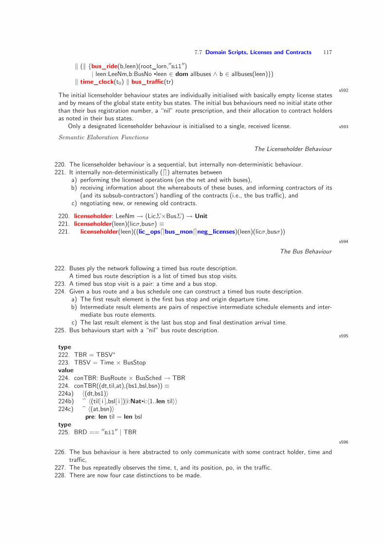
7.7 Domain Scripts, Licenses and Contracts 117
‖ (‖ bus ride(b,leen)(root lorn,′′nil′′)| leen:LeeNm,b:BusNo •leen ∈ dom allbuses ∧ b ∈ allbuses(leen))
‖ time clock(t0) ‖ bus traffic(tr)s592
The initial licenseholder behaviour states are individually initialised with basically empty license statesand by means of the global state entity bus states. The initial bus behaviours need no initial state otherthan their bus registration number, a “nil” route prescription, and their allocation to contract holdersas noted in their bus states.
Only a designated licenseholder behaviour is initialised to a single, received license. s593
Semantic Elaboration Functions
The Licenseholder Behaviour
220. The licenseholder behaviour is a sequential, but internally non-deterministic behaviour.221. It internally non-deterministically (⌈⌉) alternates between
a) performing the licensed operations (on the net and with buses),b) receiving information about the whereabouts of these buses, and informing contractors of its
(and its subsub-contractors’) handling of the contracts (i.e., the bus traffic), andc) negotiating new, or renewing old contracts.
220. licenseholder: LeeNm → (LicΣ×BusΣ) → Unit221. licenseholder(leen)(licσ,busσ) ≡221. licenseholder(leen)((lic ops⌈⌉bus mon⌈⌉neg licenses)(leen)(licσ,busσ))
s594
The Bus Behaviour
222. Buses ply the network following a timed bus route description.A timed bus route description is a list of timed bus stop visits.
223. A timed bus stop visit is a pair: a time and a bus stop.224. Given a bus route and a bus schedule one can construct a timed bus route description.
a) The first result element is the first bus stop and origin departure time.b) Intermediate result elements are pairs of respective intermediate schedule elements and inter-
mediate bus route elements.c) The last result element is the last bus stop and final destination arrival time.
225. Bus behaviours start with a “nil” bus route description.s595
type222. TBR = TBSV∗
223. TBSV = Time × BusStopvalue224. conTBR: BusRoute × BusSched → TBR224. conTBR((dt,til,at),(bs1,bsl,bsn)) ≡224a) 〈(dt,bs1)〉224b) 〈(til[ i ],bsl[ i ])|i:Nat•i:〈1..len til〉〉224c) 〈(at,bsn)〉
pre: len til = len bsltype225. BRD == ′′nil′′ | TBR
s596
226. The bus behaviour is here abstracted to only communicate with some contract holder, time andtraffic,
227. The bus repeatedly observes the time, t, and its position, po, in the traffic.228. There are now four case distinctions to be made.

118 7 Domain Engineering
229. If the bus is idle (and a a bus stop) then it waits for a next route, brd′ on which to engage.230. If the bus is at the destination of its journey then it so informs its owner (i.e., the sub-contractor)
and resumes being idle.231. If the bus is ‘en route’, at a bus stop, then it so informs its owner and continues the journey.232. In all other cases the bus continues its journey
s597
value226. bus ride: leen:LeeNm × bno:Bno → (LicNm × BRD) →226. in,out l to b[ leen,bno ], in,out b to tr[ bno ], in b to t[ bno ] Unit226. bus ride(leen,bno)(licn,brd) ≡227. let t = b to t[ bno ]? in227. let (bus,pos) = (b to tr[ bno ]!reqBusAndPos(bno,t) ; b to tr[ bno ]?) in228. case (brd,pos) of229. (′′nil′′,mkAtBS( , , , )) →229. let (licn,brd′) = (l to b[ leen,bno ]!reqBusRid(pos);l to b[ leen,bno ]?) in229. bus ride(leen,bno)(licn,brd′) end230. (〈(at,pos)〉,mkAtBS( , , , )) →230s l to b[ l,b ]!BusΣMsg(t,pos);230 l to b[ l,b ]!BusHistΣMsg(licn,bno);230 l to b[ l,b ]!FreeΣ ActΣMsg(licn,bno) ;230 bus ride(leen,bno)(ilicn,′′nil′′),231. (〈(t,pos),(t′,bs′)〉brd′,mkAtBS( , , , )) →231s l to b[ l,b ]!BusΣMsg(t,pos) ;231 bus ride(licn,bno)(〈(t′,bs′)〉brd′),232. → bus ride(leen,bno)(licn,brd) end end end
s598In formula line 227 of bus ride we obtained the bus. But we did not use “that” bus ! We we maywish to record, somehow, number of passengers alighting and boarding at bus stops, bus fees paid,one way or another, etc. The bus, which is a time-dependent entity, gives us that information. Thuswe can revise formula lines 230s and 231s:
Simple: 230s l to b[ l,b ]!BusΣMsg(pos);Revised: 230r l to b[ l,b ]!BusΣMsg(pos,bus info(bus));
Simple: 231s l to b[ l,b ]!BusΣMsg(pos);Revised: 231r l to b[ l,b ]!BusΣMsg(pos,bus info(bus));
typeBus Info = Passengers × Passengers × Cash × ...
valuebus info: Bus → Bus Infobus info(bus) ≡ (obs alighted(bus),obs boarded(bus),obs till(bus),...)
It is time to discuss our description (here we choose the bus ride behaviour) in the light of our claimof modeling “the domain”. These are our comments:
• First one should recognise, i.e., be reminded, that the narrative and formal descriptions are alwaysabstractions. That is, they leave out few or many things. We, you and I, shall never be able todescribe everything there is to describe about even the simplest entity, operation, event or behaviour.
•••
s599
The Global Time Behaviour

7.7 Domain Scripts, Licenses and Contracts 119
233. The time clock is a never ending behaviour — started at some time t0.234. The time can be inquired at any moment by any of the licenseholder behaviours and by any of the
bus behaviours.235. At any moment the time clock behaviour may not be inquired.236. After a skip of the clock or an inquiry the time clock behaviour continues, non-deterministically
either maintaining the time or advancing the clock!s600
value233. time clock: T →233. in,out l to t[ leen ] | leen:LeeNm • leen ∈ leenms233. in,out b to t[ bno ] | bno:BusNo • bno ∈ busnos Unit233. time clock:(t) ≡235. (skip ⌈⌉234. (⌈⌉⌊⌋l to t[ leen ]? ; l to t[ leen ]!t | leen:LeeNm•leen ∈ leens)234. ⌈⌉ (⌈⌉⌊⌋b to t[ bno ]? ; b to t[ bno ]!t | bno:BusNo•bno ∈ busnos)) ;236. (time clock:(t) ⌈⌉ time clock(t+δt))
s601
The Bus Traffic Behaviour
237. There is a single bus traffic behaviour. It is, “mysteriously”, given a constant argument, “the”traffic, tr.
238. At any moment it is ready to inform of the position, bps(b), of a bus, b, assumed to be in thetraffic at time t.
239. The request for a bus position comes from some bus.240. The bus positions are part of the traffic at time t.241. The bus traffic behaviour, after informing of a bus position reverts to “itself”.
s602
value237. bus traffic: TR → in,out b to tr[ bno ]|bno:BusNo•bno ∈ busnos Unit237. bus traffic(tr) ≡239. ⌈⌉⌊⌋ let reqBusAndPos(bno,time) = b to tr[ b ]? in assert b=bno238. if time 6∈ dom tr then chaos else240. let ( ,bps) = tr(t) in238. if bno 6∈ dom tr(t) then chaos else238. b to tr[ bno ]!bps(bno) end end end end | b:BusNo•b ∈ busnos ;241. bus traffic(tr)
s603
License Operations
242. The lic ops function models the contract holder choosing between and performing licensed oper-ations.We remind the reader of the four actions that licensed operations may give rise to; cf. the abstractsyntax of actions, Page 110.
243. To perform any licensed operation the sub-contractor needs to know the time and244. must choose amongst the four kinds of operations that are licensed. The choice function, which we
do not define, makes a basically non-deterministic choice among licensed alternatives. The choiceyields the contract number of a received contract and, based on its set of licensed operations, ityields either a simple action or a sub-contracting action.
245. Thus there is a case distinction amongst four alternatives.246. This case distinction is expressed in the four lines identified by: 246.247. All the auxiliary functions, besides the action arguments, require the same state arguments.
s604

120 7 Domain Engineering
value242. lic ops: LeeNm → (LicΣ×BusΣ) → (LicΣ×BusΣ)242. lic ops(leen)(licσ,busσ) ≡243. let t = (time channel(leen)!req Time;time channel(leen)?) in244. let (licn,act) = choice(licσ)(busσ)(t) in245. (case act of246. mkCon(blid,bid) → cndct(licn,leenm,t,act),246. mkCan(blid,bid) → cancl(licn,leenm,t,act),246. mkIns(blid,bid) → insrt(licn,leenm,t,act),246. mkLic(leenm′,bo) → sublic(licn,leenm,t,act) end)(licσ,busσ) end end
cndct,cancl,insert: SmpAct→(LicΣ×BusΣ)→(LicΣ×BusΣ)sublic: SubLic→(LicΣ×BusΣ)→(LicΣ×BusΣ)
s605
Bus Monitoring
Like for the bus ride behaviour we decompose the bus monitoring behaviour into two behaviours.The local bus monitoring behaviour monitors the buses that are commissioned by the sub-contractor.The licensor bus monitoring behaviour monitors the buses that are commissioned by sub-contractorssub-contractd by the contractor.
valuebus mon: l:LeeNm → (LicΣ×BusΣ)
→ in l to b[ l,b ]|b:BNo•b ∈ allbuses(l) (LicΣ×BusΣ)bus mon(l)(licσ,busσ) ≡
local bus mon(l)(licσ,busσ) ⌈⌉ licensor bus mon(l)(licσ,busσ)
s606
248. The local bus monitoring function models all the interaction between a contract holder and itsdespatched buses.
249. We show only the communications from buses to contract holders.250.251.252.253.254.255.256.257.258.
s607
248. local bus mon: leen:LeeNm → (LicΣ×BusΣ)249. → in l to b[ leen,b ]|b:BNo•b ∈ allbuses(l) (LicΣ×BusΣ)248. local bus mon(leen)(licσ:(rlσ,slσ,lbσ),busσ:(fbσ,abσ)) ≡250. let (bno,msg) = ⌈⌉⌊⌋(b,l to b[ l,b ]?)|b:BNo•b ∈ allbuses(leen) in254. let (blid,bid,licn,lorn,trace) = abσ(bno) in251. case msg of252. BusΣMsg(t,bs) →256. let abσ′ = update BusΣ(bno)(licn,leen,blid,bid)(t,bs)(abσ) in256. (licσ,(fbσ,abσ′,histσ)) end,258. BusHistΣMsg(licn,bno) →258. let lbσ′ =258. update LorBusΣ(obs LorNm(licn),licn,leen,(blid,bid),(b,trace))(lbσ) in258. l to l[ leen,obs LorNm(licn) ]!Licensor BusHistΣMsg(licn,leen,bno,blid,bid,tr);

7.7 Domain Scripts, Licenses and Contracts 121
258. ((rlσ,slσ,lbσ′),busσ) end257. FreeΣ ActΣMsg(licn,bno)→258. let (fbσ′,abσ′) = update FreeΣ ActΣ(bno,bs)(fbσ,abσ) in258. (licσ,(fbσ′,abσ′)) end258. end end end
s608
259.260.261.262.263.
s609
259. licensor bus mon: lorn:LorNm → (LicΣ×BusΣ)259. → in l to l[ lorn,leen ]|leen:LeeNm•leen ∈ leenms\lorn (LicΣ×BusΣ)259. licensor bus mon(lorn)(licσ,busσ) ≡259. let (rlσ,slσ,lbhσ) = licσ in259. let (leen,Licensor BusHistΣMsg(licn,leen′′,bno,blid,bid,tr))
= ⌈⌉⌊⌋(leen′,l to l[ lorn,leen′ ]?)|leen′:LeeNm•leen′ ∈ leenms\lorn in259. let lbhσ′ =259. update BusHistΣ(obs LorNm(licn),licn,leen′′,(blid,bid),(bno,trace))(lbhσ) in259. l to l[ leenm,obs LorNm(licnm) ]!Licensor BusHistΣMsg(b,blid,bid,lin,lee,tr);259. ((rlσ,slσ,lbhσ′),busσ)259. end end end
s610
License Negotiation
264.265.266.267.268.269.270.271.272.273.274.275.
s611
264.265.266.267.268.269.270.271.272.273.274.
s612
The Conduct Bus Ride Action

122 7 Domain Engineering
276. The conduct bus ride action prescribed by (ln,mkCon(bli,bi,t′) takes place in a context and shallhave the following effect:a) The action is performed by contractor li and at time t. This is known from the context.b) First it is checked that the timetable in the contract named ln does indeed provide a journey,
j, indexed by bli and (then) bi, and that that journey starts (approximately) at time t′ whichis the same as or later than t.
c) Being so the action results in the contractor, whose name is “embedded” in ln, receivingnotification of the bus ride commitment. s613
d) Then a bus, selected from a pool of available buses at the bust stop of origin of journey j,is given j as its journey script, whereupon that bus, as a behaviour separate from that ofsub-contractor li, commences its ride.
e) The bus is to report back to sub-contractor li the times at which it stops at en route bus stopsas well as the number (and kind) of passengers alighting and boarding the bus at these stops.
f) Finally the bus reaches its destination, as prescribed in j, and this is reported back to sub-contractor li.
g) Finally sub-contractor li, upon receiving this ‘end-of-journey’ notification, records the bus asno longer in actions but available at the destination bus stop.
s614
276.276a)276b)276c)276d)276e)276f)276g)
s615
The Cancel Bus Ride Action
277. The cancel bus ride action prescribed by (ln,mkCan(bli,bi,t′) takes place in a context and shallhave the following effect:a) The action is performed by contractor li and at time t. This is known from the context.b) First a check like that prescribed in Item 276b) is performed.c) If the check is OK, then the action results in the contractor, whose name is “embedded” in ln,
receiving notification of the bus ride cancellation.That’s all !
s616
277.277a)277b)277c)
s617
The Insert Bus Ride Action
278. The insert bus ride action prescribed by (ln,mkIns(bli,bi,t′) takes place in a context and shall havethe following effect:a) The action is performed by contractor li and at time t. This is known from the context.b) First a check like that prescribed in Item 276b) is performed.c) If the check is OK, then the action results in the contractor, whose name is “embedded” in ln,
receiving notification of the new bus ride commitment.d) The rest of the effect is like that prescribed in Items 276d)–276g).
s618

7.8 Domain Human Behaviour 123
278.278a)278b)278c)278d)
s619
The Contracting Action
279. The subcontracting action prescribed by (ln,mkLic(li′,(pe′,ops′,tt′))) takes place in a context andshall have the following effect:a) The action is performed by contractor li and at time t. This is known from the context.b) First it is checked that timetable tt is a subset of the timetable contained in, and that the
operations ops are a subset of those granted by, the contract named ln.c) Being so the action gives rise to a contract of the form (ln′,li,(pe′,ops′,tt′),li′). ln′ is a unique
new contract name computed on the basis of ln, li, and t. li′ is a sub-contractor name chosenby contractor li. tt′ is a timetable chosen by contractor li. ops′ is a set of operations likewisechosen by contractor li.
d) This contract is communicated by contractor li to sub-contractor li′.e) The receipt of that contract is recorded in the license state.f) The fact that the contractor has sublicensed part (or all) of its obligation to conduct bus rides
is recorded in the modified component of its received contracts.s620
279.279a)279b)279c)279d)279e)279f)
s621
Discussion This ends Example 65acm-tsode-3
7.7.1 Principles s622
7.7.2 Discussion s623
7.8 Domain Human Behaviour s624
acm-tsode-4
Definition 57 – Human Behaviour: By human behaviour we mean any of a quality spectrumof carrying out assigned work: from (i) careful, diligent and accurate, via (ii) sloppy dispatch,and (iii) delinquent work, to (iv) outright criminal pursuit.
s625
Example 66 – A Casually Described Bank Script: Our formulation amounts to just a (casual)rough sketch. It is followed by a series of three larger examples (Examples 67–69). Each of theseelaborate on the theme of (bank) scripts.
The problem area is that of how repayments of mortgage loans are to be calculated. At any onetime a mortgage loan has a balance, a most recent previous date of repayment, an interest rate and ahandling fee. When a repayment occurs, then the following calculations shall take place: (i) the interest s626
on the balance of the loan since the most recent repayment, (ii) the handling fee, normally consideredfixed, (iii) the effective repayment — being the difference between the repayment and the sum of theinterest and the handling fee — and the new balance, being the difference between the old balanceand the effective repayment. s627

124 7 Domain Engineering
We assume repayments to occur from a designated account, say a demand/deposit account. Weassume that bank to have designated fee and interest income accounts.
(i) The interest is subtracted from the mortgage holder’s demand/deposit account and added tothe bank’s interest (income) account. (ii) The handling fee is subtracted from the mortgage holder’sdemand/deposit account and added to the bank’s fee (income) account. (iii) The effective repaymentis subtracted from the mortgage holder’s demand/deposit account and also from the mortgage bal-ance. Finally, one must also describe deviations such as overdue repayments, too large, or too smalls628
repayments, and so on. This ends Example 66s629
Example 67 – A Formally Described Bank Script: First we must informally and formally definethe bank state:
There are clients (c:C), account numbers (a:A), mortgage numbers (m:M), account yields (ay:AY)and mortgage interest rates (mi:MI). The bank registers, by client, all accounts (ρ:A Register) andall mortgages (µ:M Register). To each account number there is a balance (α:Accounts). To eachmortgage number there is a loan (ℓ:Loans). To each loan is attached the last date that interest waspaid on the loan.
s630
valuer, r′:Real axiom ...
typeC, A, M, DateAY′ = Real, AY = | ay:AY′
• 0<ay≤r |MI′ = Real, MI = | mi:MI′ • 0<mi≤r′ |Bank′ = A Register × Accounts × M Register × LoansBank = | β:Bank′ • wf Bank(β)|A Register = C →m A-setAccounts = A →m BalanceM Register = C →m M-setLoans = M →m (Loan × Date)Loan,Balance = PP = Nat
s631Then we must define well-formedness of the bank state:
valueay:AY, mi:MI
wf Bank: Bank → Boolwf Bank(ρ,α,µ,ℓ) ≡ ∪ rng ρ = dom α ∧ ∪ rng µ = dom ℓ
axiomay<mi [ ∧ ... ]
s632We — perhaps too rigidly — assume that mortgage interest rates are higher than demand/depositaccount interest rates: ay<mi.
Operations on banks are denoted by the commands of the bank script language. First the syntax:
typeCmd = OpA | CloA | Dep | Wdr | OpM | CloM | PayOpA == mkOA(c:C)CloA == mkCA(c:C,a:A)Dep == mkD(c:C,a:A,p:P)Wdr == mkW(c:C,a:A,p:P)OpM == mkOM(c:C,p:P)Pay == mkPM(c:C,a:A,m:M,p:P,d:Date)

7.8 Domain Human Behaviour 125
CloM == mkCM(c:C,m:M,p:P)Reply = A | M | P | OkNokOkNok == ok | notok
valueperiod: Date × Date → Days [ for calculating interest ]before: Date × Date → Bool [ first date is earlier than last date ]
s633And then the semantics:
int Cmd(mkPM(c,a,m,p,d))(ρ,α,µ,ℓ) ≡let (b,d′) = ℓ(m) inif α(a)≥p
thenlet i = interest(mi,b,period(d,d′)),
ℓ′ = ℓ † [ m 7→ℓ(m)−(p−i) ]α′ = α † [ a 7→α(a)−p,ai 7→α(ai)+i ] in
((ρ,α′,µ,ℓ′),ok) endelse
((ρ,α′,µ,ℓ),nok)end endpre c ∈ dom µ ∧ a ∈ dom α ∧ m ∈ µ(c)post before(d,d′)
interest: MI × Loan × Days → P
This ends Example 67s634
Example 68 – Bank Staff or Programmer Behaviour: Let us assume a bank clerk, “in ye olde”days, when calculating, say mortgage repayments (cf. Example 67).
We would characterise such a clerk as being diligent, etc., if that person carefully follows themortgage calculation rules, and checks and double-checks that calculations “tally up”, or lets others doso. We would characterise a clerk as being sloppy if that person occasionally forgets the checks alludedto above. We would characterise a clerk as being delinquent if that person systematically forgets thesechecks. And we would call such a person a criminal if that person intentionally miscalculates in such away that the bank (and/or the mortgage client) is cheated out of funds which, instead, may be divertedto the cheater. s635
Let us, instead of a bank clerk, assume a software programmer charged with implementing anautomatic routine for effecting mortgage repayments (cf. Example 67).
We would characterise the programmer as being diligent if that person carefully follows the mort-gage calculation rules, and throughout the development verifies and tests that the calculations arecorrect with respect to the rules. We would characterise the programmer as being sloppy if that personforgets certain checks and tests when otherwise correcting the computing program under development.We would characterise the programmer as being delinquent if that person systematically forgets thesechecks and tests. And we would characterise the programmer as being a criminal if that person in-tentionally provides a program which miscalculates the mortgage interest, etc., in such a way that thebank (and/or the mortgage client) is cheated out of funds. This ends Example 68
s636
Example 69 – A Human Behaviour Mortgage Calculation: Example 67 gave a semantics to themortgage calculation request (i.e., command) as would a diligent bank clerk be expected to performit. To express, that is, to model, how sloppy, delinquent, or outright criminal persons (staff?) couldbehave we must modify the int Cmd(mkPM(c,a,m,p,d′))(ρ,α,µ,ℓ) definition.
int Cmd(mkPM(c,a,m,p,d))(ρ,α,µ,ℓ) ≡let (b,d′) = ℓ(m) in

126 7 Domain Engineering
if q(α(a),p) /∗ α(a)≤p∨α(a)=p∨α(a)≤p∨... ∗/then
let i = f1(interest(mi,b,period(d,d′))),ℓ′ = ℓ † [ m 7→f2(ℓ(m)−(p−i)) ]α′ = α † [ a 7→f3(α(a)−p),ai 7→f4(α(ai)+i),
a“staff” 7→f“staff”(α(a“staff”)+i) ] in((ρ,α′,µ,ℓ′),ok) end
else((ρ,α′,µ,ℓ),nok)
end endpre c ∈ dom µ ∧ m ∈ µ(c)
q: P × P∼→ Bool
f1,f2,f3,f4,f“staff”: P∼→ P [ typically: f“staff” = λp.p ]
s637The predicate q and the functions f1, f2, f3, f4 and f“staff” of Example 67 are deliberately left un-defined. They are being defined by the “staffer” when performing (incl., programming) the mortgagecalculation routine.
The point of Example 67 is that one must first define the mortgage calculation script precisely asone would like to see the diligent staff (programmer) to perform (incl., correctly program) it before onecan “pinpoint” all the places where lack of diligence may “set in”. The invocations of q, f1, f2, f3, f4
and f“staff” designate those places.The point of Example 67 is also that we must first domain-define, “to the best of our ability” all
the places where human behaviour may play other than a desirable role. If we cannot, then we cannotclaim that some requirements aim at countering undesirable human behaviour. This endsExample 69
s638
Example 70 – Transport Net Building:We show the example in two stages: First we show a description of a diligent operation; then of a
less careful operation.
Sub-example 1 (of Example 70 – ) A Diligent Operation: The int Insert operation of Example 10Page 11 was expressed without stating necessary pre-conditions:
11 23 The insert operation takes an Insert command and a net and yields either a new net or chaos forthe case where the insertion command “is at odds” with, that is, is not semantically well-formedwith respect to the net. s639
12 We characterise the “is not at odds”, i.e., is semantically well-formed, that is: pre int Insert(op)(hs,ls),as follows: it is a propositional function which applies to Insert actions, op, and nets, (hs.ls), andyields a truth value if the below relation between the command arguments and the net is satisfied.Let (hs,ls) be a value of type N.
13 If the command is of the form 2oldH(hi′,l,hi′) then⋆1 hi′ must be the identifier of a hub in hs,⋆2 l must not be in ls and its identifier must (also) not be observable in ls, and⋆3 hi′′ must be the identifier of a(nother) hub in hs.
s640
14 If the command is of the form 1oldH1newH(hi,l,h) then⋆1 hi must be the identifier of a hub in hs,⋆2 l must not be in ls and its identifier must (also) not be observable in ls, and⋆3 h must not be in hs and its identifier must (also) not be observable in hs.
15 If the command is of the form 2newH(h′,l,h′′) then⋆1 h′ — left to the reader as an exercise (see formalisation !),
23See Page 13 for Item 11 et cetera.

7.8 Domain Human Behaviour 127
⋆2 l — left to the reader as an exercise (see formalisation !), and⋆3 h′′ — left to the reader as an exercise (see formalisation !).
s641
value12′ pre int Insert: Ins → N → Bool12′′ pre int Insert(Ins(op))(hs,ls) ≡⋆2 s l(op)6∈ ls ∧ obs LI(s l(op)) 6∈ iols(ls) ∧
case op of13 2oldH(hi′,l,hi′′) → hi′,hi′′⊆iohs(hs),14 1oldH1newH(hi,l,h)→ hi ∈ iohs(hs)∧h 6∈ hs∧obs HI(h)6∈ iohs(hs),15 2newH(h′,l,h′′) → h′,h′′∩ hs=∧obs HI(h′),obs HI(h′′)∩ iohs(hs)=
end
These must be carefully expressed and adhered to in order for staff to be said to carry out the linkinsertion operation accurately. This ends Sub-example 70.1
s642
Sub-example 2 (of Example 70 – ) A Sloppy via Delinquent to Criminal Operation: We replacesystematic checks (∧) with partial checks (∨), etcetera, and obtain various degrees of sloppy todelinquent, or even criminal behaviour.
value12′ pre int Insert: Ins → N → Bool12′′ pre int Insert(Ins(op))(hs,ls) ≡⋆2 s l(op)6∈ ls ∧ obs LI(s l(op)) 6∈ iols(ls) ∧
case op of13 2oldH(hi′,l,hi′′) → hi′ ∈ iohs(hs)∨hi′′isin iohs(hs),14 1oldH1newH(hi,l,h)→ hi ∈ iohs(hs)∨h 6∈ hs∨obs HI(h)6∈ iohs(hs),15 2newH(h′,l,h′′) → h′,h′′∩ hs=∨obs HI(h′),obs HI(h′′)∩ iohs(hs)=
end
This ends Sub-example 70.2
This ends Example 70
7.8.1 A Meta Characteristic of Human Behaviour s643
Commensurate with the above, humans interpret rules and regulations differently, and not alwaysconsistently — in the sense of repeatedly applying the same interpretations. s644
Schema 3 – A Human Behaviour Specification Pattern:
type
[ 1 ] α: Action = Σ∼→ Σ-infset
value[ 2 ] hum int: Rule → Σ → RUL-infset[ 3 ] action: Stimulus → Σ → Σ
[ 4 ] hum beha: Stimulus × Rules → Action → Σ∼→ Σ-infset
[ 5 ] hum beha(sy sti,sy rul)(α)(σ) as σset[ 6 ] post[ 7 ] σset = α(σ) ∧ action(sy sti)(θ) ∈ θset[ 8 ] ∧ ∀ σ′:Σ•σ′ ∈ σset ⇒[ 9 ] ∃ se rul:RUL•se rul ∈ hum int(sy rul)(σ)⇒se rul(σ,σ′)

128 7 Domain Engineering
s645
The above is, necessarily, sketchy: [1] There is a possibly infinite variety of ways of interpretingsome rules. [2] A human, in carrying out an action, interprets applicable rules and chooses onewhich that person believes suits some (professional, sloppy, delinquent or criminal) intent. “Suits”means that it satisfies the intent, i.e., yields true on the pre/post-configuration pair, when theaction is performed — whether as intended by the ones who issued the rules and regulations ornot. We do not cover the case of whether an appropriate regulation is applied or not.
The above-stated axioms express how it is in the domain, not how we would like it to be. Forthat we have to establish requirements.
7.8.2 Principles s646
7.8.3 Discussion s647
7.9 Opening and Closing Stages s648
acm-tsode-e
We cover in this section the following aspects of domain engineering:
• opening stages (Sect. 7.9.1);• closing stages (Sect. 7.9.2); and• domain engineering documentation — (Sect. 7.9.3).
Sections
7.9.1 Opening Stages s649
For completeness, we shall briefly list the opening stages of domain engineering. They are:
1. domain stake-holder identification (and subsequent liaison);2. rough sketching of business processes;3. domain acquisition literature study, Internet study, on-site interviews, questionnaire prepara-
tion, questionnaire fill-in, and questionnaire handling — resulting in a great number of domaindescription units;
4. domain analysis (based on domain description units) and concept formation, and5. domain “terminologisation”.
Stakeholder Identification and Liaison s650
Domain Acquisition s651
Domain Analysis s652
Terminoligisation s653
7.9.2 Closing Stages s654
For completeness, we shall, as in Sect. 7.9.1, briefly list the closing stages of domain engineering.They are:
1. domain verification, model checking and testing – the assurance of properties of the formalisationof the domain model (Sect. 7.9.2);
2. domain validation – the assurance of the veracity of the informal, i.e., the narrative domaindescription (Sect. 7.9.2); and
3. domain theory formation (Sect. 7.9.2).
Other than this brief mentioning we shall not cover these, from an engineering view-point ratherimportant stages — but refer to [19].

7.10 Exercises 129
Verification, Model Checking and Testing s655
Domain Validation s656
Domain Theory s657
7.9.3 Domain Engineering Documentation s658
7.9.4 Conclusion s659
7.10 Exercises
See Items 11–18 (of Appendix D, starting Page 231).


Part V
Requirements


8
Requirements Engineering
s660 acm-rtre-a
8.1 Characterisations
Definition 58 – IEEE Definition of ‘Requirements’: By a requirements we understand (cf.IEEE Standard 610.12 [85]): “A condition or capability needed by a user to solve a problem orachieve an objective”.
s661
Principle 4 – Requirements Engineering [1]: Prescribe only those requirements that can beobjectively shown to hold for the designed software.
Principle 5 – Requirements Engineering [2]: When prescribing requirements, formulate, atthe same time, tests (theorems, properties for model checking) whose actualisation should showadherence to the requirements
s662
Definition 59 – Requirements: By requirements we shall understand a document which pre-scribes desired properties of a machine: (i) what entities the machine shall “maintain”, and whatthe machine shall (must; not should) offer of (ii) functions and of (iii) behaviours (iv) while alsoexpressing which events the machine shall “handle”.
s663
A requirements prescription ideally specifies externally observable properties of simple entities,functions, events and behaviours of the machine such as the requirements stake-holders wishthem to be. s664
Above we used the term ‘ideally’. Even in good practice the requirements engineer may, hereand there in the requirements prescription, resort to prescribe the requirements more by how iteffects the what rather than only (i.e., ‘ideally’) prescribe the requirements by what the machineis to offer. s665
The machine is what is required, that is, the hardware and software that is to be designedand which are to satisfy the requirements.
It is a highlight of this document that requirements engineering has a scientific foundationand that that scientific foundation is the domain theory, that is the properties of the domain asmodelled by a domain description. s666
Conventional requirements engineering, as covered in a great number of software engineeringtextbooks [65, 116, 118, 136, 143], does not have (such) a scientific foundation. This foundationallows us to pursue requirements engineering in quite a new manner.
The key idea of the kind of requirements engineering that we shall present is that a major partof the requirements can be systematically “derived” from a description of the domain in which therequirements ‘reside’.

134 8 Requirements Engineering
8.2 The Core Stages of Requirements Engineering s667
The core stages of requirements engineering are therefore those of ‘deriving’ the following re-quirements facets: business process re-engineering (Sect. 8.5), domain requirements1 (Sect. 8.6 onpage 141), interface requirements2 (Sect. 8.8 on page 153) and machine requirements3 (Sect. 8.9on page 165).
8.3 On Opening and Closing Requirements Engineering Stages s668
We refer to Sect. 8.10.
8.4 Requirements Acquisition s669
acm-rtre-a
Requirements ‘reside’ in the domain. That means: one can not possibly utter a reasonably com-prehensive set of requirements without stating the domain “to which they apply”. Therefore wefirst describe the domain before we next prescribe the requirements. And therefore we shall “baseour requirements acquisition” on a supposedly existing domain description.s670
To ‘base our requirements acquisition . . . etc.’ shall mean that we carefully go through thedomain description (found most appropriate for the requirements at hand) with the requirementsstake-holders asking them a number of questions. Which these questions are will be dealt withsoon.
For domain acquisition there were, in principle, no prior domain description documents, really,to refer to. Hence an elaborate set of procedures had to be followed in order to solicit and elicitdomain acquisition units. Before such elicitation could be done in any systematic fashion thedomain engineer had to study the domain, by whatever informal means available. Now there isthe domain description.s671
From a purely linguistic point of view we can think of decomposing requirements acquisitionrelative to the domain description along three axes: the first axis of domain requirements — beingthose which can be expressed solely using terms from the domain; the second axis of machinerequirements — being those which can be expressed solely using terms from the machine; and thethird axis of interface requirements — being those which can be expressed using terms from boththe domain and the machine.
The next three sections, Sects. 8.6–8.9, shall therefore be structured into two parts: the respec-tive requirements acquisition part and the corresponding requirements modelling part.acm-bpr
8.5 Business Process Re-Engineering s672
We remind the reader of Sect. 7.2 (in which we covered the concept of ‘business processes’).
Definition 60 – Business Process Re-Engineering: By business process re-engineering we un-derstand the reformulation of previously adopted business process descriptions, together with ad-ditional business process engineering work.
s673
Business process re-engineering (BPR) is about change, and hence BPR is also about changemanagement. The concept of workflow is one of these “hyped” as well as “hijacked” terms: Theysound good, and they make you “feel” good. But they are often applied to widely different subjects,albeit having some phenomena in common. By workflow we shall, very loosely, understand thephysical movement of people, materials, information and “centre (‘locus’) of control” in someorganisation (be it a factory, a hospital or other).
1Domain requirements are in conventional textbooks referred to as functional requirements2Interface requirements are in conventional textbooks referred, more-or-less, to as user requirements.3Machine requirements are in conventional textbooks referred, more-or-less, to as system requirements.

8.5 Business Process Re-Engineering 135
8.5.1 Michael Hammer’s Ideas on BPR s674
Michael Hammer, a guru of the business process re-engineering “movement”, states [69]:
1. Understand a method of re-engineering before you do it for serious.
So that is what this section is about.
2. One can only re-engineer processes.
Clearly Hammer utters an untenable dogma. We ma-u also need to re-engineer such phenomenaas simple entities and functions.
3. Understanding the process is an essential first step in re-engineering.
And then he goes on to say: “but an analysis of those processes is a waste of time. You mustplace strict limits, both on time you take to develop this understanding and on the length of thedescription you make.” Needless to say we question this latter part of the third item.
4. If you proceed to re-engineer without the proper leadership, you are making a fatal mistake.If your leadership is nominal rather than serious, and isn’t prepared to make the requiredcommitment, your efforts are doomed to failure.
By leadership is basically meant: “upper, executive management”.
5. Re-Engineering requires radical, breakthrough ideas about process design. Re-Engineeringleaders must encourage people to pursue stretch goals4 and to think out of the box; to thisend, leadership must reward creative thinking and be willing to consider any new idea. s675
This is clearly an example of the US guru, “new management”-type ‘speak’ !
6. Before implementing a process in the real world create a laboratory version in order to testwhether your ideas work. . . . Proceeding directly from idea to real-world implementation is(usually) a recipe for disaster.
Our careful both informal and formal description of the existing domain processes, as covered inSect. 7, as well as the similarly careful prescription of the re-engineered business processes shall,in a sense, make up for this otherwise vague term “laboratory version”.
7. You must re-engineer quickly. If you can’t show some tangible results within a year, you willlose the support and momentum necessary to make the effort successful. To this end “scopecreep” must be avoided at all cost. Stay focused and narrow the scope if necessary in order toget results fast.
We obviously do not agree, in principle and in general, with this statement.
8. You cannot re-engineer a process in isolation. Everything must be on the table. Any attemptsto set limits, to preserve a piece of the old system, will doom your efforts to failure.
We can only agree. But the wording is like mantras. As a software engineer, founded in science,such statements as the above are not technical, are not scientific. They are “management speak”.
9. Re-Engineering needs its own style of implementation: fast, improvisational, and iterative.
We are not so sure about this statement either! Professional engineering work is something oneneither does fast nor improvisational.
10. Any successful re-engineering effort must take into account the personal needs of the individualsit will affect. The new process must offer some benefit to the people who are, after all, beingasked to embrace enormous change, and the transition from the old process to the new onemust be made with great sensitivity as to their feelings.
4A ‘stretch goal’ is a goal, an objective, for which, if one wishes to achieve that goal, one has to stretchoneself.

136 8 Requirements Engineering
This is nothing but a politically correct, pat statement! It would not pass the negation test: Nobodywould claim the opposite. Real benefits of re-engineering often come from not requiring as manypeople, i.e., workers and management, in the corporation as before re-engineering. Hence: Whatabout the “feelings” of those laid off?
8.5.2 What Are BPR Requirements? s676
Two “paths” lead to business process re-engineering:
• A client wishes to improve enterprise operations by deploying new computing systems (i.e.,new software). In the course of formulating requirements for this new computing system aneed arises to also re-engineer the human operations within and without the enterprise.
• An enterprise wishes to improve operations by redesigning the way staff operates within the en-terprise and the way in which customers and staff operate across the enterprise-to-environmentinterface. In the course of formulating re-engineering directives a need arises to also deploy newsoftware, for which requirements therefore have to be enunciated.
One way or the other, business process re-engineering is an integral component in deploying newcomputing systems.
8.5.3 Overview of BPR Operations s677
We suggest six domain-to-business process re-engineering operations. They are based on the facetsthat were prominent in the process of constructing a domain description.
1. introduction of some new and removal of some old intrinsics;2. introduction of some new and removal of some old support technologies;3. introduction of some new and removal of some old management and organisation substruc-
tures;4. introduction of some new and removal of some old rules and regulations;5. related scripting; and6. introduction of some new and removal of some old work practices (relating to human be-
haviours);
8.5.4 BPR and the Requirements Document s678
Requirements for New Business Processes
The reader must be duly “warned”: The BPR requirements are not for a computing system, butfor the people who “surround” that (future) system. The BPR requirements state, unequivocally,how those people are to act, i.e., to use that system properly. Any implications, by the BPRrequirements, as to concepts and facilities of the new computing system must be prescribed (also)in the domain and interface requirements.
Place in Narrative Document s679
We shall thus, in Sects. 8.5.5–8.5.9, treat a number of BPR facets. Each of whatever you decideto focus on, in any one requirements development, must be prescribed. And the prescription mustbe put into the overall requirements prescription document.s680
As the BPR requirements “rebuilds” the business process description part of the domain de-scription5, and as the BPR requirements are not directly requirements for the machine, we findthat they (the BPR requirements texts) can be simply put in a separate section.s681
5— Even if that business process description part of the domain description is “empty” or nearly so!

8.5 Business Process Re-Engineering 137
There are basically two ways of “rebuilding” the domain description’s business process’s de-scription part (DBP ) into the requirements prescription part’s BPR requirements (RBPR). Eitheryou keep all of D as a base part in RBPR, and then you follow that part (i.e., RBPR) with state-ments, R′
BPR, that express the new business process’s “differences” with respect to the “old”(DBP ). Call the result RBPR. Or you simply rewrite (in a sense, the whole of) DBP directly into s682
RBPR, copying all of DBP , and editing wherever necessary.
Place in Formalisation Document s683
The above statements as how to express the “merging” of BPR requirements into the overallrequirements document apply to the narrative as well as to the formalised prescriptions.
Principle 6 – Documentation: We may assume that there is a formal domain description, DBP ,(of business processes) from which we develop the formal prescription of the BPR requirements.We may then decide to either develop entirely new descriptions of the new business processes, s684
i.e., actually prescriptions for the business re-engineered processes, RBPR; or develop, from DBP ,using a suitable schema calculus, such as the one in RSL, the requirements prescription RBPR, bysuitable parameterisation, extension, hiding, etc., of the domain description DBP .
8.5.5 Intrinsics Review and Replacement s685
Definition 61 – Intrinsics Review and Replacement: By intrinsics review and replacement weunderstand an evaluation as to whether current intrinsics stays or goes, and as to whether newerintrinsics need to be introduced.
s686
Example 71 – Intrinsics Replacement: A railway net owner changes its business from owning,operating and maintaining railway nets (lines, stations and signals) to operating trains. Hence themore detailed state changing notions of rail units need no longer be part of that new company’sintrinsics while the notions of trains and passengers need be introduced as relevant intrinsics.
Replacement of intrinsics usually point to dramatic changes of the business and are usually notdone in connection with subsequent and related software requirements development.
8.5.6 Support Technology Review and Replacement s687
Definition 62 – Support Technology Review and Replacement: By support technology reviewand replacement we understand an evaluation as to whether current support technology as used inthe enterprise is adequate, and as to whether other (newer) support technology can better performthe desired services.
s688
Example 72 – Support Technology Review and Replacement: Currently the main informationflow of an enterprise is taken care of by printed paper, copying machines and physical distribution. Allsuch documents, whether originals (masters), copies, or annotated versions of originals or copies, aresubject to confidentiality. As part of a computerised system for handling the future information flow,it is specified, by some domain requirements, that document confidentiality is to be taken care of byencryption, public and private keys, and digital signatures. However, it is realised that there can bea need for taking physical, not just electronic, copies of documents. The following business process s689
re-engineering proposal is therefore considered:Specially made printing paper and printing and copyingmachines are to be procured, and so are printers and copiers whose use requires the insertion of specialsignature cards which, when used, check that the person printing or copying is the person identifiedon the card, and that that person may print the desired document. All copiers will refuse to copysuch copied documents — hence the special paper. Such paper copies can thus be read at, but notcarried outside the premises (of the printers and copiers). And such printers and copiers can register

138 8 Requirements Engineering
who printed, respectively who tried to copy, which documents. Thus people are now responsible forthe security (whereabouts) of possible paper copies (not the required computing system). The above, s690
somewhat construed example, shows the “division of labour” between the contemplated (required,desired) computing system (the “machine”) and the “business re-engineered” persons authorised toprint and possess confidential documents.
It is implied in the above that the re-engineered handling of documents would not be feasiblewithout proper computing support. Thus there is a “spill-off” from the business re-engineered worldto the world of computing systems requirements.
8.5.7 Management and Organisation Re-Engineering s691
Definition 63 – Management and Organisation Re-Engineering: By management and organ-isation re-engineering we understand an evaluation as to whether current management principlesand organisation structures as used in the enterprise are adequate, and as to whether other man-agement principles and organisation structures can better monitor and control the enterprise.
s692
Example 73 – Management and Organisation Re-Engineering: A rather complete comput-erisation of the procurement practices of a company is being contemplated. Previously procurementwas manifested in the following physically separate as well as designwise differently formatted paperdocuments: requisition form, order form, purchase order, delivery inspection form, rejection and returnform, and payment form. The supplier had corresponding forms: order acceptance and quotation form,delivery form, return acceptance form, invoice form, return verification form, and payment acceptanceform. The current concern is only the procurement forms, not the supplier forms. The proposed domains693
requirements are mandating that all procurer forms disappear in their paper version, that basically onlyone, the procurement document, represents all phases of procurement, and that order, rejection andreturn notification slips, and payment authorisation notes, be effected by electronically communicatedand duly digitally signed messages that represent appropriate subparts of the one, now electronic pro-curement document. The business process re-engineering part may now “short-circuit” previous staff’ss694
review and acceptance/rejection of former forms, in favour of fewer staff interventions.The new business procedures, in this case, subsequently find their way into proper domain require-
ments: those that support, that is monitor and control all stages of the re-engineered procurementprocess.
8.5.8 Rules and Regulations Re-Engineering s695
Definition 64 – Rules and Regulation Re-Engineering: By rules and regulations re-engineeringwe understand an evaluation as to whether current rules and regulations as used in the enterpriseare adequate, and as to whether other rules and regulations can better guide and regulate theenterprise.
Here it should be remembered that rules and regulations principally stipulate business engineeringprocesses. That is, they are — i.e., were — usually not computerised.s696
Example 74 – Rules and Regulations Re-Engineering: Our example continues that of Example 60on page 97. We kindly remind the reader to re-study that example. Assume now, due to re-engineeredsupport technologies, that interlock signalling can be made magnitudes safer than before, withoutinterlocking. Thence it makes sense to re-engineer the rule of Example 60 from: In any three-minuteinterval at most one train may either arrive to or depart from a railway station into: In any 20-secondinterval at most two trains may either arrive to or depart from a railway station.
This re-engineered rule is subsequently made into a domain requirements, namely that the softwaresystem for interlocking is bound by that rule.

8.5 Business Process Re-Engineering 139
8.5.9 Script Re-Engineering s697
On one hand, there is the engineering of the contents of rules and regulations, and, on anotherhand, there are the people (management, staff) who script these rules and regulations, and theway in which these rules and regulations are communicated to managers and staff concerned. s698
Definition 65 – Script Re-Engineering: By script re-engineering we understand evaluation asto whether the way in which rules and regulations are scripted and made known (i.e., posted) tostakeholders in and of the enterprise is adequate, and as to whether other ways of scripting andposting are more suitable for the enterprise.
s699
Example 75 – Health-care Script Re-Engineering: We refer to Example 63 (Pages 103–105). Letus assume that the situation before this business re-engineering process starts, in relation to hospitalhealth-care, was that there was no physically visible notion of a health-care license language, but the therequirements now calls for such a language to be introduced with as much computer & communicationsupport as is reasonable and that the hospital(s) in question are to become “paper-less”. Now we canforesee a number of business process re-engineering based on the concept that such a health-care licenselanguage has been designed. For every action performed by a medical staff, whether an admittance, s700
annamnese, planning analysis, carrying out our analysis, diagnostics, treatment planning, treatment(in all forms), et cetera, action (cf. Fig. 7.10 on page 104), there now has to be prescribed, by andfor the hospital health-care staff a BPR prescription, which outlines what the staff members must doin preparation of the action, the action (probably nothing new here), and in concluding the action sothat the medical staff performs the necessary “chores” assumed by the health-care license languagesoftware.
8.5.10 Human Behaviour Re-Engineering s701
Definition 66 – Human Behaviour Re-Engineering: By human behaviour re-engineering weunderstand an evaluation as to whether current human behaviour as experienced in the enterpriseis acceptable, and as to whether partially changed human behaviours are more suitable for theenterprise.
s702
Example 76 – Human Behaviour Re-Engineering: A company has experienced certain lax atti-tudes among members of a certain category of staff. The progress of certain work procedures thereforeis re-engineered, implying that members of another category of staff are henceforth expected to followup on the progress of “that” work.
In a subsequent domain requirements stage the above re-engineering leads to a number of require-ments for computerised monitoring of the two groups of staff.
8.5.11 A Specific Example of BPR s703
Example 77 – A Toll-road System (I):Example 10 (Pages 9–17) outline a generic model of a domain of roads (links) and their intersections
(hubs). We shall base some of the requirements examples of Sect. 8 on an instantiation of that domainmodel (Example 10) to a specific toll-road system. In this example we shall rough sketch that toll-roadsystem. First we refer to Fig. 8.1 on the following page. s704
s705We first explain the kind of toll-roads semi-generically hinted at by Fig. 8.1 on the next page.The core of the (semi-generic) toll-road is the “linear” stretch of pairs of one-way links (ℓjj+1
, ℓj+1j)
between adjacent hubs hj and hj+1. This is the actual toll-road. In order to enter and leave the toll-roadthere are entries and exits. These are in the form of toll plazas tpi. Simple two-way links, ℓj, connecttoll plaza tpj (via toll plaza intersection tij to toll-road intersection hj . s706
We must here state that toll plazas are equipped with toll booths for cars entering the toll-roadsystem and for cars leaving the toll-road system.

140 8 Requirements Engineering
tp1 tp2 tp3 tpntpn−1tpj
l12
l32
l23 l34 lj−1j
ljj−1l43 lj+1j
ljj+1
ln−1n−2
ln−1n
lnn−1
ln−2n−1
l21
l1 l2 l3 lj ln−1 ln
h2h1 h3 hj hn−1 hn
Fig. 8.1. A simple, linear toll road net:tpi: tboll plaza i,ti1, tin: terminal (or toll plaza) intersection k,hk: intermediate intersection (hub) k, 1<k<nℓi: toll plaza link i,lxy: toll-way link from ix to iy , y=x+1 or y=x-1 and 1≤x<n.
The basic business process of this toll-road system includes (i) the maintenance of all roads, inter-sections and toll plaza toll booths; (ii) the travel, through the toll-road system of a toll-paying car; and(iii) the monitoring and control of toll-paying car traffic within the toll-road system. s707
We shall only summarise the travel (i) business process: (1) A car enters the toll-road system at tollplaza tpi. (2) A toll booth gate prevents the car from fully entering the system. (3) The car is issueda toll slip by an entry toll-booth at toll plaza tpi. (4) The toll-booth gate allows the car from enteringthe system. (5) The car travels along toll plaza link ℓj to toll-road hub hj . [Let, in the following hj
now be hi.] (6) At toll-road hub hi the car decides whether to continue driving along the toll-roads708
proper or to leave the toll-road system along toll plaza link ℓj to toll plaza tpi. In the latter case thebusiness process description continues with Item (8). (7) The car travels, along toll-road link eitherℓii+1
or ℓii−1, between toll-road hub hi and hub hi+1 respectively hub hi+−. [Let, in the following this
target hub now be hi.] The next business process step is now described in Item (6). (8) At toll plazatpi the car enters an exit toll-booth. (9) A toll-booth gate prevents the car from leaving the toll-roadsystem. (10) The previously issued toll slip is now presented at the toll-booth. (11) The toll-booths709
calculates the fare from entry plaza to exit plaza6. (13) The car (driver) somehow7 (14) The toll-boothgate allows the car to leave the toll-road system. (15) The car leaves the toll-road system.
This ends Example 77
8.5.12 Discussion: Business Process Re-Engineering s710
Who Should Do the Business Process Re-Engineering?
It is not in our power, as software engineers, to make the kind of business process re-engineeringdecisions implied above. Rather it is, perhaps, more the prerogative of appropriately educated,trained and skilled (i.e., gifted) other kinds of engineers or business people to make the kinds ofdecisions implied above. Once the BP re-engineering has been made, it then behooves the clientstakeholders to further decide whether the BP re-engineering shall imply some requirements, ornot.s711
Once that last decision has been made in the affirmative, we, as software engineers, can thenapply our abstraction and modelling skills, and, while collaborating with the former kinds ofprofessionals, make the appropriate prescriptions for the BPR requirements. These will typicallybe in the form of domain requirements, which are covered extensively in Sect. 8.6.
6We shall not detail this calculation. Its proper calculation may involve that the system has traced thecar’s passage through all hubs.
7We shall not detail that “somehow”: whether it is by cash payment, via credit card, or by means ofa toll-road system credit mechanism “built-into” the car.

8.6 Domain Requirements 141
General s712
Business process re-engineering is based on the premise that corporations must change their wayof operating, and, hence, must “reinvent” themselves. Some corporations (enterprises, businesses,etc.) are “vertically” structured along functions, products or geographical regions. This oftenmeans that business processes “cut across” vertical units. Others are “horizontally” structuredalong coherent business processes. This often means that business processes “cut across” functions,products or geographical regions. In either case adjustments may need to be made as the business(i.e., products, sales, markets, etc.) changes. We otherwise refer to currently leading books onbusiness process re-engineering: [68, 69, 84, 89].
8.6 Domain Requirements s713
acm-rtre-b
8.6.1 A Small Domain Example
In exemplifying several of the very many kinds of domain and machine requirements we need asmall domain description. This small domain description will be that of a timetable, cf. Exam-ple 78. The sequence of machine requirements examples based on Example 78 will, furthermore,be expressed using the scheme and class modularisation constructs of RSL. s714
tt0
Example 78 – A Domain Example: an ‘Airline Timetable System’:We choose a very simple domain: that of a traffic timetable, say flight timetable. In the domain
you could, in “ye olde days”, hold such a timetable in your hand, you could browse it, you could lookup a special flight, you could tear pages out of it, etc. There was no end as to what you could do tosuch a timetable. So we will just postulate a sort, TT, of timetables. s715
Airline customers, clients, in general, only wish to inquire a timetable (so we will here omit treatmentof more or less “malicious” or destructive acts). But you could still count the number of digits “7” inthe timetable, and other such ridiculous things. So we postulate a broadest variety of inquiry functions,qu:QU, that apply to timetables, tt:TT, and yield values, val:VAL. s716
Specifically designated airline staff may, however, in addition to what a client can do, update thetimetable. But, recalling human behaviours, all we can ascertain for sure is that update functions,up:UP, apply to timetables and yield two things: another, replacement timetable, tt:TT, and a result,res:RES, such as: “your update succeeded”, or “your update did not succeed”, etc. In essence this isall we can say for sure about the domain of timetable creations and uses. s717
We can view the domain of the timetable, clients and staff as a behaviour which nondeterministicallyalternates (⌈⌉) between the client querying the timetable client 0(tt), and the staff updating the samestaff 0(tt). s718
scheme TI TBL 0 =class
typeTT, VAL, RESQU = TT → VALUP = TT → TT × RES
valueclient 0: TT → VAL, client 0(tt) ≡ let q:QU in q(tt) endstaff 0: TT → TT × RES, staff 0(tt) ≡ let u:UP in u(tt) end
tim tbl 0: TT → Unittim tbl 0(tt) ≡
(let v = client 0(tt) in tim tbl 0(tt) end)⌈⌉ (let (tt′,r) = staff 0(tt) in tim tbl 0(tt′) end)
end

142 8 Requirements Engineering
The timetable function, tim tbl, is here seen as a never ending process, hence the type Unit. Itnondeterministically8 alternates between “serving” the clients and the staff. Either of these two non-deterministically chooses from a possibly very large set of queries, respectively updates.
This ends Example 78
8.6.2 Acquisition s719
acm-rtre-b
Common to the acquisition and modelling of domain requirements are the following sub-stages:
• projection,
• instantiation,
• determination,
• extension and
• fitting.
sub-stages.
With each and every stake-holder group the domain engineer(s) go through the domain de-scription and asks the following questions:
• Which of the simple entities, functions, events and behaviour (parts) of the domain do youwish to be represented somehow in, i.e., projected onto the machine ?s720
• Which of the simple entities, functions, events and behaviour (parts) of the domain do youwish to be less generic, more instantiated in the machine ?
• Which of the simple entities, functions, events and behaviour (parts) of the domain do youwish to appear more deterministic in the machine ?
• Are there simple entities, functions, events and behaviours that could be in the domain but arenot there because their “existence” is not feasible — if so, with computing and communicationare they now feasible and should the domain thus be extended ?
• Given that there may be several, parallel ongoing requirements development for related partsof the domain, should they be fitted ?
s721
For each of these five sub-stages of domain requirements the acquisition consists in asking thesequestions and marking the domain description cum emerging domain requirements document withthe answers:
• circling-in the domain description parts that are to be part of the domain requirements (i.e.,projection)
• marking those parts with possible directives as to instantiation and determination;• making adequate notes on possible extensions• and fittings.
Once this domain requirements acquisition has taken place for all groups of stake-holders therequirements engineers can proceed to interface requirements acquisition, Sect. 8.8.1.
8.6.3 Projection s722
Definition 67 – Projection: By domain projection we understand an operation that appliesto a domain description and yields a domain requirements prescription. The latter represents aprojection of the former in which only those parts of the domain are present that shall be of interestin the ongoing requirements development
s723arms-projection
Example 79 – Projection: A Road Maintenance System: The requirements are for a road main-tenance system. That is, maintenance of link and hub (road segment and road intersection) surfaces,the monitoring of their quality and road repair.
8The nondeterminism referred to is internal in the sense that no outside behaviour influences thechoice.
9Formula numbers refer to narrative text items as from Page 9 etc.

8.6 Domain Requirements 143
Instead of listing all the phenomena and concepts of the domain that are “projected away”, we listthose few that remain: hubs, links, hub identifiers and link identifiers; nets, corresponding observerfunctions, and corresponding axioms.
s724
type1: H, L,9
2: N = H-set × L-setaxiom
2: ∀ (hs,ls):N • card hs≥2 ∧ card ks≥1type
3: HI, LIvalue
4a: obs HI: H → HI, obs LI: L → LIaxiom
4b: ∀ h,h′:H, l,l′:L • h 6=h′
⇒ obs HI(h)6=obs HI(h′) ∧ l 6=l′⇒obs LI(l)6=obs LI(l′)
s725
value5a: obs HIs: L → HI-set6a: obs LIs: H → LI-set5b: ∀ l:L • card obs HIs(l)=2 ∧6b: ∀ h:H • card obs LIs(h)≥1 ∧5a: ∀ (hs,ls):N • ∀ h:H • h ∈ hs ⇒ ∀ li:LI • li ∈ obs LIs(h) ⇒
∃ l′:L • l′ ∈ ls ∧ li=obs LI(l′) ∧ obs HI(h) ∈ obs HIs(l′) ∧6a: ∀ l:L • l ∈ ls ⇒
∃ h′,h′′:H • h′,h′′⊆hs ∧ obs HIs(l)=obs HI(h′),obs HI(h′′)7: ∀ h:H • h ∈ hs ⇒ obs LIs(h) ⊆ iols(ls)8: ∀ l:L • l ∈ ls ⇒ obs HIs(h) ⊆ iohs(hs)
iohs: H-set → HI-set, iols: L-set → LI-setiohs(hs) ≡ obs HI(h)|h:H•h ∈ hsiols(ls) ≡ obs LI(l)|l:L•l ∈ ls
This ends Example 79s726acm-rtre-b
atrs-projectionExample 80 – Projection: A Toll-road System: For the ‘Toll-road System’, as outlined in Ex-ample 77, in addition to what was projected for the ‘Road Maintenance System’ of Example 79, thefollowing entities and most related functions are projected: hubs, links, hub and link identifiers; nets,that is, hub state and hub state spaces and link states and link state spaces, corresponding observerfunctions, corresponding axioms and syntactic and semantic wellformedness predicates.
s727
typeLΣ′ = L Trav-setL Trav = (HI × LI × HI)LΣ = | lnkσ:LΣ′
• syn wf LΣlnkσ |HΣ′ = H Trav-setH Trav = (LI × HI × LI)HΣ = | hubσ:HΣ′
• wf HΣhubσ |HΩ = HΣ-set, LΩ = LΣ-set
valueobs HΣ: H → HΣ, obs LΣ: L → LΣobs HΩ: H → HΩ, obs LΩ: L → LΩ

144 8 Requirements Engineering
axiom∀ h:H • obs HΣ(h) ∈ obs HΩ(h) ∧ ∀ l:L • obs LΣ(l) ∈ obs LΩ(l)
For hubs, links, hub identifiers and link identifiers and nets see the above projection; and for the missingaxioms and wellformedness predicates see Example 58 (Pages 89–91).
This ends Example 80
8.6.4 Instantiation s728
acm-rtre-b
Definition 68 – Instantiation: By domain instantiation we understand an operation that appliesto a (projected and possibly determined) domain description, i.e., a requirements prescription, andyields a domain requirements prescription, where the latter has been made more specific, usuallyby constraining a domain description
s729arms-
instantiation Example 81 – Instantiation: A Road Maintenance System: We continue Example 79.
11. The road net consist of a sequence of one or more road segments.12. A road segment can be characterised by a pair of hubs and a pair of links connected to these hubs.13. Neighbouring road segments share a hub.14. All hubs are otherwise distinct.15. All links are distinct.16. The two links of a road segment connects to the hubs of the road segment.17. We can show that road nets are specific instances of concretisations of the former, thus more
abstract road nets.
s730
type11 RN = RS∗,12 RS = H × (L × L) × Haxiom∀ rn:RN •
13 ∀ i:Nat • i,i+1⊆inds rn ⇒ let ( , ,h)=rn(i),(h′, , )=rn(i+1) in h=h′ end ∧14 len rn + 1 = cardh,h′|h,h′:H•(h, ,h′)∈ elems rn ∧15 2∗(len rn) = cardl,l′|l,l′:L•( ,(l,l′), )∈ elems rn ∧16 ∀ (h,(l,l′),h′):RS • (h,(l,l′),h′) ∈ elems rn ⇒
obs Σ(l)=(obs HI(h),obs HI(h′)) ∧ obs Σ(l′)=(obs HI(h′),obs HI(h))value17 abs N: RN → N
abs N(rsl) ≡(h,h′|(h, ,h′):RS • (h, ,h′) ∈ elems rsl,l,l′|( ,(,l,l′), ):RS • ( .(l,l′), ) ∈ elems rsl)
This ends Example 81s731acm-rtre-b
atrs-instantiation Example 82 – Instantiation: A Toll-road System: We continue Example 80. The 1st versiondomain requirements prescription, Example 80, is now updated with respect to the properties of thetoll-road net: We refer to Fig. 8.1 on page 140 and the preliminary description given in Example 77.There are three kinds of hubs: tollgate hubs and intersection hubs: terminal intersection hubs andproper, intermediate intersection hubs. Tollgate hubs have one connecting two way link. linking thetollgate hub to its associated intersection hub. s732Terminal intersection hubs have threeconnecting links: (i) one, a two-way link, to a tollgate hub, (ii) one one-way link emanating to a nextup (or down) intersection hub, and (iii) one one-way link incident upon this hub from a next up (ordown) intersection hub. Proper intersection hubs have five connecting links: one, a two way link, to atollgate hub, two one way links emanating to next up and down intersection hubs, and two one way

8.6 Domain Requirements 145
links incident upon this hub from next up and down intersection hub. (Much more need be narrated.)As a result we obtain a 2nd version domain requirements prescription.
s733
typeTN = ((H × L) × (H × L × L))∗ × H × (L × H)
valueabs N: TN → Nabs N(tn) ≡ (tn hubs(tn),tn hubs(tn))pre wf TN(tn)
tn hubs: TN → H-set,tn hubs(hll,h,( ,hn)) ≡h,hn ∪ thj,hj|((thj,tlj),(hj,lj,lj′)):((H×L)×(H×L×L))•((thj,tlj),(hj,lj,lj′))∈ elems hlll
tn links: TN → L-settn links(hll, ,(ln, )) ≡ln ∪ tlj,lj,lj′|((thj,tlj),(hj,lj,lj′)):((H×L)×(H×L×L))•((thj,tlj),(hj,lj,lj′))∈ elems hlll
theorem ∀ tn:TN • wf TN(tn) ⇒ wf N(abs N(tn))
s734
typeLnkM == plaza | way
valuewf TN: TN → Boolwf TN(tn:(hll,h,(ln,hn))) ≡
wf Toll Lnk(h,ln,hn)(plaza) ∧ wf Toll Ways(hll,h) ∧wf State Spaces(tn) [ to be defined under Determination ]
wf Toll Ways: ((H×L)×(H×L×L))∗ × H → Boolwf Toll Ways(hll,h) ≡∀ j:Nat • j,j+1⊆inds hll ⇒
let ((thj,tlj),(hj,ljj′,lj′j)) = hll(j),( ,(hj′, , )) = hll(j+1) inwf Toll Lnk(thj,tlj,hj)(plaza) ∧wf Toll Lnk(hj,ljj′,hj′)(way) ∧ wf Toll Lnk(hj′,lj′j,hj)(way) end ∧let ((thk,tlk),(hk,lk,lk′)) = hll(len hll) inwf Toll Lnk(thk,tlk,hk)(plaza) ∧wf Toll Lnk(hk,lk,hk′)(way) ∧ wf Toll Lnk(hk′,lk′,hk)(way) end
s735
wf Toll Lnk: (H×L×H) → LnkM → Boolwf Toll Lnk(h,l,h′)(m) ≡
obs Ps(l)=(obs HI(h),obs LI(l),obs HI(h′)),(obs HI(h′),obs LI(l),obs HI(h)) ∧obs Σ(l) = case m of
plaza → obs Ps(l),way → (obs HI(h),obs LI(l),obs HI(h′)) end
This ends Example 82
8.6.5 Determination s736acm-rtre-b
Definition 69 – Determination: By domain determination we understand an operation thatapplies to a (projected) domain description, i.e., a requirements prescription, and yields a domainrequirements prescription, where the latter has made deterministic, or specific, some functionresults or some behaviours of the former

146 8 Requirements Engineering
s737tt1-dd
Example 83 – Timetable System Determination: We make airline timetables more specific,tt0-dd
more deterministic. There are given notions of departure and arrival times, and of airports, and ofairline flight numbers.s738
scheme TI TBL 2 =extend TI TBL 1 with
classtype
T, An, Fnend
s739A timetable consists of a number of air flight journey entries. Each entry has a flight number, and alist of two or more airport visits. an airport visit consists of three parts: An airport name, and a pair of(gate) arrival and departure times.s740
scheme TI TBL 3 =extend TI TBL 2 with
classtype
JR′ = (T × An × T)∗
JR = | jr:JR′• len jr ≥ 2 ∧ ... |
TT = Fn →m JRend
We illustrate just one, simple form of airline timetable queries. A simple airline timetable query eitherjust browses all of an airline timetable, or inquires of the journey of a specific flight. The simple browses741
query thus need not provide specific argument data, whereas the flight journey query needs to providea flight number. A simple update query inserts a new pairing of a flight number and a journey to thetimetable, whereas a delete query need just provide the number of the flight to be deleted.s742
The result of a query is a value: the specific journey inquired, or the entire timetable browsed. Theresult of an update is a possible timetable change and either an “OK” response if the update couldbe made, or a “Not OK” response if the update could not be made: Either the flight number of thejourney to be inserted was already present in the timetable, or the flight number of the journey to bedeleted was not present in the timetable.s743
That is, we assume above that simple airline timetable queries only designate simple flights, withone aircraft. For more complex air flights, with stopovers and changes of flights, see Sect. 86 onpage 149.
You may skip the rest of the example, its formalisation, if your reading of this paper does notinclude the various formalisations. First, we formalise the syntactic and the semantic types:
scheme TI TBL 3Q =extend TI TBL 3 with
classtype
Query == mk brow() | mk jour(fn:Fn)Update == mk inst(fn:Fn,jr:JR) | mk delt(fn:Fn)VAL = TTRES == ok | not ok
end
Then we define the semantics of the query commands:s744
scheme TI TBL 3U =extend TI TBL 3 with
class

8.6 Domain Requirements 147
valueMq: Query → QUMq(qu) ≡
case qu ofmk brow() → λtt:TT•tt,mk jour(fn)→ λtt:TT • if fn ∈ dom tt
then [ fn 7→tt(fn) ] else [ ] endend end
And, finally, we define the semantics of the update commands: s745
scheme TI TBL 3U =extend TI TBL 3 with
classMu: Update → UPMu(up) ≡
case qu ofmk inst(fn,jr) → λtt:TT •
if fn ∈ dom ttthen (tt,not ok) else (tt ∪ [ fn 7→jr ],ok) end,
mk delt(fn) → λtt:TT •
if fn ∈ dom ttthen (tt \ fn,ok) else (tt,not ok) end
end end
We can “assemble” the above into the timetable function — calling the new function the timetablesystem, or just the system function. s746
Before we had:
valuetim tbl 0: TT → Unittim tbl 0(tt) ≡
(let v = client 0(tt) in tim tbl 0(tt) end)⌈⌉ (let (tt′,r) = staff 0(tt) in tim tbl 0(tt′) end)
Now we get:
valuesystem: TT → Unitsystem() ≡
(let q:Query in let v =Mq(q)(tt) in system(tt) end end)⌈⌉ (let u:Update in let (r,tt′) =Mu(q)(tt) in system(tt′) end end)
s747Or, for use in Example 99:
system(tt) ≡ client(tt) ⌈⌉ staff(tt)
client: TT → Unitclient(tt) ≡
let q:Query in let v =Mq(q)(tt) in system(tt) end end
staff: TT → Unitstaff(tt) ≡
let u:Update in let (r,tt′) =Mu(q)(tt) in system(tt′) end end

148 8 Requirements Engineering
We remind the reader that the above example can be fully understood by just reading the rough-sketch texts, that is, without reading their formalisations.
This ends Example 83s748acm-rtre-b
arms-
determination
Example 84 – Determination: A Road Maintenance System: We continue Example 81.Weshall, in this example, claim that the following items constitute issues of more determinate nature ofthe ‘Road Management System’ under development. fixing the states of links and hubs; endowing linksand hubs with such attributes as road surface material (concrete, asphalt, etc.), state of road surfacewear-and-tear, hub and link areas, say in m2, time units needed for and cost of ordinary cleaning ofm2s of hub and link surface; time units needed for and cost of ordinary repairs of m2s of hub and linksurface; etcetera.s749
18. The two links of a road segment are open for traffic in one direction and in opposite directionsonly.
19. Hubs are always in the same state, namely one that allows traffic from incoming links to continueonto all outgoing links.
20. Hubs and Links have a number of attributes that allow for the monitoring and planning of hub andlink surface conditions, i.e., whether in ordinary or urgent need of cleaning and/or repair.
s750
axiom∀ rn:RN •
18 ∀ (h,(l,l′),h′):RS • (h,(l,l′),h′) ∈ elems rn ⇒obs LΣl(l) = (obs HI(h),obs LI(l),obs HI(h′)) ∧obs LΣl(l′) = (obs HI(h′),obs LI(l′),obs HI(h)) ∧
19 ∀ i:Nat • i,i+1⊆inds rn •
let ((h,(l,l′),h′),(h′,(l′′,l′′′),h′′)) = (rn(i),rn(i+1)) incase i of
1 → obs HΣ(h) = (obs LI(l),obs HI(h),obs LI(l′)),len rn → obs HΣ(h′) = (obs LI(l′),obs HI(h′),obs LI(l)),→ obs HΣ(h′)
= (obs LI(l),obs HI(h′),obs LI(l′)),(obs LI(l),obs HI(h′),obs LI(l′))end end
type20 Surface, WearTear, Area, OrdTime, OrdCost, RepTime, RepCost, ...value20 obs Surface: (H|L)→Surface, obs WearTear: (H|L)→WearTear, ...
This ends Example 84s751acm-rtre-b
atrs-
determination
Example 85 – Determination: A Toll-road System: We continue Example 82. We single out onlytwo ’determinations’: The link state spaces. There is only one link state: the set of all paths throughthe link, thus any link state space is the singleton set of its only link state. The hub state spaces arethe singleton sets of the “current” hub states which allow these crossings: (i) from terminal link backto terminal link, (ii) from terminal link to emanating tollway link, (iii) from incident tollway link toterminal link, and (iv) from incident tollway link to emanating tollway link. Special provision must bemade for expressing the entering from the outside and leaving toll plazas to the outside.s752
wf State Spaces: TN → Boolwf State Spaces(hll,hn,(thn,tln)) ≡
let ((th1,tl1),(h1,l12,l21)) = hll(1),((thk,ljk),(hk,lkn,lnk)) = hll(len hll) in
wf Plaza(th1,tl1,h1) ∧ wf Plaza(thn,tln,hn) ∧wf End(h1,tl1,l12,l21,h2) ∧ wf End(hk,tln,lkn,lnk,hn) ∧

8.6 Domain Requirements 149
∀ j:Nat • j,j+1,j+2⊆inds hll ⇒let (,(hj,ljj,lj′j)) = hll(j),((thj′,tlj′),(hj′,ljj′,lj′j′)) = hll(j+1) inwf Plaza(thj′,tlj′,hj′) ∧ wf Interm(ljj,lj′j,hj′,tlj′,ljj′,lj′j′) end end
wf Plaza(th,tl,h) ≡obs HΣ(th) = [ crossings at toll plazas ](external,obs HI(th),obs LI(tl)),
(obs LI(tl),obs HI(th),external),(obs LI(tl),obs HI(th),obs LI(tl)) ∧
obs HΩ(th)=obs HΣ(th) ∧obs LΩ(tl) = obs LΣ(tl)
s753
wf End(h,tl,l,l′) ≡obs HΣ(h) = [ crossings at 3−link end hubs ](obs LI(tl),obs HI(h),obs LI(tl)),(obs LI(tl),obs HI(h),obs LI(l)),(obs LI(l′),obs HI(h),obs LI(tl)),(obs LI(l′),obs HI(h),obs LI(l)) ∧
obs HΩ(h) = obs HΣ(h) ∧obs LΩ(l) = obs LΣ(l) ∧ obs LΩ(l′) = obs LΣ(l′)
wf Interm(ul 1,dl 1,h,tl,ul,dl) ≡obs HΣ(h) = [ crossings at properly intermediate, 5−link hubs ]
(obs LI(tl),obs HI(h),obs LI(tl)),(obs LI(tl),obs HI(h),obs LI(dl 1)),(obs LI(tl),obs HI(h),obs LI(ul)),(obs LI(ul 1),obs HI(h),obs LI(tl)),(obs LI(ul 1),obs HI(h),obs LI(ul)),(obs LI(ul 1),obs HI(h),obs LI(dl 1)),(obs LI(dl),obs HI(h),obs LI(tl)),(obs LI(dl),obs HI(h),obs LI(dl 1)),(obs LI(dl),obs HI(h),obs LI(ul)) ∧obs HΩ(h) = obs HΣ(h) ∧ obs LΩ(tl) = obs LΣ(tl) ∧obs LΩ(ul) = obs LΣ(ul) ∧ obs LΩ(dl) = obs LΣ(dl)
Not all determinism issues above have been fully explained. But for now we should — in principle —be satisfied. This ends Example 85
8.6.6 Extension s754
acm-rtre-b
Definition 70 – Extension: By domain extension we understand an operation that applies to a(projected and possibly determined and instantiated) domain description, i.e., a (domain) require-ments prescription, and yields a (domain) requirements prescription. The latter prescribes thata software system is to support, partially or fully, an operation that is not only feasible but alsocomputable in reasonable time
s755tt1-de
Example 86 – Timetable System Extension:We assume a projected and instantiated timetable (see Sect. 83 on page 146).A query of a timetable may, syntactically, specify an airport of origin, ao, an airport of destination,
ad, and a maximum number, n, of intermediate stops. The query semantically designates the set of allthose trips of one up to n direct air journeys between ao and ad, i.e., trips where the passenger maychange flights (up to n− 1 times) at intermediate airports. s756
scheme TI TBL 3C =extend TI TBL 3 with
classtype
Query′ == Query | mk conn(fa:An,ta:An,n:Nat)VAL′ = VAL | CNS
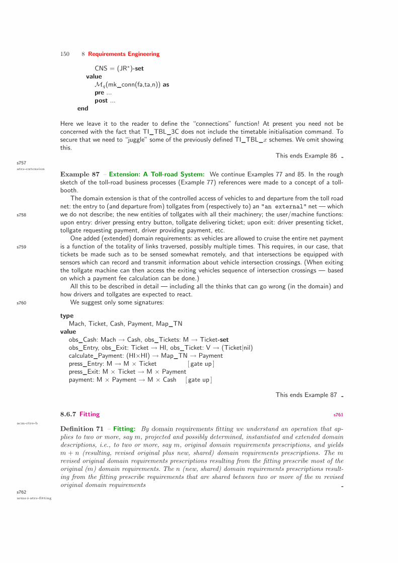
150 8 Requirements Engineering
CNS = (JR∗)-setvalueMq(mk conn(fa,ta,n)) aspre ...post ...
end
Here we leave it to the reader to define the “connections” function! At present you need not beconcerned with the fact that TI TBL 3C does not include the timetable initialisation command. Tosecure that we need to “juggle” some of the previously defined TI TBL x schemes. We omit showingthis.
This ends Example 86s757atrs-extension
Example 87 – Extension: A Toll-road System: We continue Examples 77 and 85. In the roughsketch of the toll-road business processes (Example 77) references were made to a concept of a toll-booth.
The domain extension is that of the controlled access of vehicles to and departure from the toll roadnet: the entry to (and departure from) tollgates from (respectively to) an "an external" net — whichwe do not describe; the new entities of tollgates with all their machinery; the user/machine functions:s758
upon entry: driver pressing entry button, tollgate delivering ticket; upon exit: driver presenting ticket,tollgate requesting payment, driver providing payment, etc.
One added (extended) domain requirements: as vehicles are allowed to cruise the entire net paymentis a function of the totality of links traversed, possibly multiple times. This requires, in our case, thats759
tickets be made such as to be sensed somewhat remotely, and that intersections be equipped withsensors which can record and transmit information about vehicle intersection crossings. (When exitingthe tollgate machine can then access the exiting vehicles sequence of intersection crossings — basedon which a payment fee calculation can be done.)
All this to be described in detail — including all the thinks that can go wrong (in the domain) andhow drivers and tollgates are expected to react.
We suggest only some signatures:s760
typeMach, Ticket, Cash, Payment, Map TN
valueobs Cash: Mach → Cash, obs Tickets: M → Ticket-setobs Entry, obs Exit: Ticket → HI, obs Ticket: V → (Ticket|nil)calculate Payment: (HI×HI) → Map TN → Paymentpress Entry: M → M × Ticket [ gate up ]press Exit: M × Ticket → M × Paymentpayment: M × Payment → M × Cash [ gate up ]
This ends Example 87
8.6.7 Fitting s761
acm-rtre-b
Definition 71 – Fitting: By domain requirements fitting we understand an operation that ap-plies to two or more, say m, projected and possibly determined, instantiated and extended domaindescriptions, i.e., to two or more, say m, original domain requirements prescriptions, and yieldsm + n (resulting, revised original plus new, shared) domain requirements prescriptions. The mrevised original domain requirements prescriptions resulting from the fitting prescribe most of theoriginal (m) domain requirements. The n (new, shared) domain requirements prescriptions result-ing from the fitting prescribe requirements that are shared between two or more of the m revisedoriginal domain requirements
s762arms+atrs-fitting
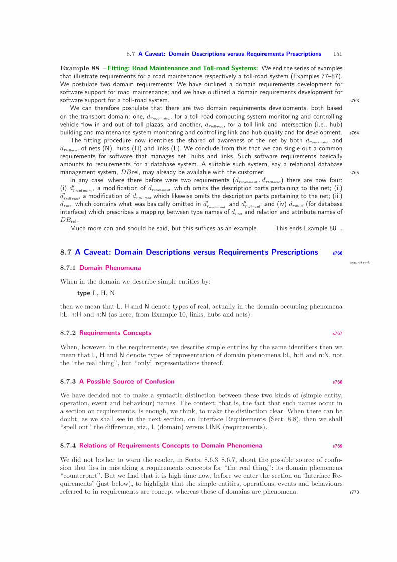
8.7 A Caveat: Domain Descriptions versus Requirements Prescriptions 151
Example 88 – Fitting: Road Maintenance and Toll-road Systems: We end the series of examplesthat illustrate requirements for a road maintenance respectively a toll-road system (Examples 77–87).We postulate two domain requirements: We have outlined a domain requirements development forsoftware support for road maintenance; and we have outlined a domain requirements development forsoftware support for a toll-road system. s763
We can therefore postulate that there are two domain requirements developments, both basedon the transport domain: one, drroad-maint., for a toll road computing system monitoring and controllingvehicle flow in and out of toll plazas, and another, drtoll-road, for a toll link and intersection (i.e., hub)building and maintenance system monitoring and controlling link and hub quality and for development. s764
The fitting procedure now identifies the shared of awareness of the net by both drroad-maint. anddrtoll-road of nets (N), hubs (H) and links (L). We conclude from this that we can single out a commonrequirements for software that manages net, hubs and links. Such software requirements basicallyamounts to requirements for a database system. A suitable such system, say a relational databasemanagement system, DBrel, may already be available with the customer. s765
In any case, where there before were two requirements (drroad-maint., drtoll-road) there are now four:(i) d′rroad-maint., a modification of drroad-maint. which omits the description parts pertaining to the net; (ii)d′rtoll-road
, a modification of drtoll-road which likewise omits the description parts pertaining to the net; (iii)drnet, which contains what was basically omitted in d′rroad-maint.
and d′rtoll-road; and (iv) drdb:i/f (for databaseinterface) which prescribes a mapping between type names of drnet and relation and attribute names ofDBrel.
Much more can and should be said, but this suffices as an example. This ends Example 88
8.7 A Caveat: Domain Descriptions versus Requirements Prescriptions s766
acm-rtre-b
8.7.1 Domain Phenomena
When in the domain we describe simple entities by:
type L, H, N
then we mean that L, H and N denote types of real, actually in the domain occurring phenomenal:L, h:H and n:N (as here, from Example 10, links, hubs and nets).
8.7.2 Requirements Concepts s767
When, however, in the requirements, we describe simple entities by the same identifiers then wemean that L, H and N denote types of representation of domain phenomena l:L, h:H and n:N, notthe “the real thing”, but “only” representations thereof.
8.7.3 A Possible Source of Confusion s768
We have decided not to make a syntactic distinction between these two kinds of (simple entity,operation, event and behaviour) names. The context, that is, the fact that such names occur ina section on requirements, is enough, we think, to make the distinction clear. When there can bedoubt, as we shall see in the next section, on Interface Requirements (Sect. 8.8), then we shall“spell out” the difference, viz., L (domain) versus LINK (requirements).
8.7.4 Relations of Requirements Concepts to Domain Phenomena s769
We did not bother to warn the reader, in Sects. 8.6.3–8.6.7, about the possible source of confu-sion that lies in mistaking a requirements concepts for “the real thing”: its domain phenomena“counterpart”. But we find that it is high time now, before we enter the section on ‘Interface Re-quirements’ (just below), to highlight that the simple entities, operations, events and behavioursreferred to in requirements are concept whereas those of domains are phenomena. s770

152 8 Requirements Engineering
The reason (for now emphasising the difference) is simple: interface requirements are aboutthe relations between phenomena of the domain and concepts of the software (being required).
When, in the domain, we name a (simple entity, operation, event or behaviour) phenomenaD, and when in the requirements, we name a corresponding (simple entity, operation, event orbehaviour) R; then, by corresponding, we mean that there is an unprovable relation
R |= D.s771
We cannot possibly formally claim that
R = D or even R ≃ D,
The R is a mathematical model of some requirements concept whereas D is thought of as “thereal thing”. Let us understand the above, seemingly contradictory statement: The D is expressedmathematically, so it must be conceptual, as is R. Therefore they ought be comparable. If wetake this view that both are mathematical models, then all is OK and we can compare them.If, however, we take the view that the names (of what is assumed, or claimed, to be domainphenomena in D) denote “the real things, out there in the actual world”, then we cannot comparethem.s772
How do we, in the following, reconcile these two views ? We do so as follows: On one hand wewrite
R |= Dto mean that the requirements abstractly models the domain, while, when we write
R abstractly refines D
or abs D(Req) = Dom we mean that the mathematical model of the requirements is a refinementof the mathematical model of the domain — in which latter phenomena names are considerednames of mathematical concepts.
8.7.5 Sort versus Type Definitions s773
As a principle we prefer to use sorts and observer functions:
Example 89 – Domain Types and Observer Functions:
typeN, L, H, LI, HI, Location, Length
valueobs Ls: N → L-set, obs Hs: N → H-setobs LI: L → LI, obs HI: H → HIobs LIs: H → LI-set, obs HIs: L → HI-setobs Location: L → Location, obs Length: L → Real
rather then type definitions:s774
Example 90 – Requirements Types and Decompositions:
typeLI, HI, Location, LengthN = L-set × H-setL = LI × (HI×HI) × Location × Length × ...H = HI × LI-set × Length × ...
value(ls,hs):N, (li,(fhi,thi),loc,len,...):L, (hi,lis,len,...):H

8.8 Interface Requirements 153
when defining simple domain entities. The type definitions are then typically introduced in re-quirements prescriptions. As shown in the last formula line of Example 90 on the preceding page,the observer functions of domain descriptions can then be simply effected by decompositions.
Discussion s775
8.8 Interface Requirements s776
acm-rtre-c
8.8.1 Acquisition s777
Interface requirements acquisition evolves around a notion of shared phenomena and concepts ofthe domain. These are listed now.
• Shared Simple Entities: The shared simple entities are those simple entities that ‘occur’ inthe domain but must also be represented by the machine.
• Shared Operations: The shared operations are those operations of the domain that can onlybe partially ‘executed’ by the machine.
• Shared Events: The shared events are those events of the domain that must be brought tothe attention of the machine.
• Shared Behaviours: The shared behaviours are those behaviours of the domain that canonly be partially ‘processed’ by the machine.
s778
Again the requirements engineers “walk” through the domain description together with each groupof requirements stake-holders marking up all the shared phenomena and concepts, and decides theirbasic principles resolution, which are duly noted in the evolving interface requirements document.
8.8.2 Shared Simple Entity Requirements s779
Definition 72 – Shared Simple Entity: By a shared simple entity we understand a simple entitythat ‘occurs’ in the domain but must also be represented by the machine.
s780shared-se-ru
Example 91 – Shared Simple Entities: Railway Units: We may think of a train traffic monitoringand control system being interface requirements developed. The following phenomena are then identifiedas among those being shared: rail units, signals, road level crossing gates, train sensors (optical sensorsensing passing trains) and trains. This ends Example 91
s781shared-se-tru
Example 92 – Shared Simple Entities: Toll-road Units: We may think of a toll-road trafficmonitoring and control system being interface requirements developed. The following phenomena areidentified as among those being shared: links, hubs, cars, (optical sensors sensing passing cars) toll-both gates, toll-booth externally arriving car sensor, toll-booth internally arriving car sensor, toll-boothrequest slip sensor and toll-booth accept slip sensor. This ends Example 92
acm-rtre
s782shared-tndrExample 93 – Shared Simple Entities: Transport Net Data Representation: We deliberately
formulated Examples 91: “Shared Simple Entities: Railway Units” and 92: “Shared Simple Entities:Toll-road Units” so as to conjure the image of two very similar set of requirements. These are nowmade into one set. In this example we focus on the machine representation of simple entities. We nowcontinue these examples as well as Example 84. s783
21. The shared simple entities are the links and the hubs. In the domain we referred to these by thesort names L and H, in the machine they will be represented by the types LINK and HUB
22. Now we must make sure that we can abstract LINK s and HUBs “back” into L and H.
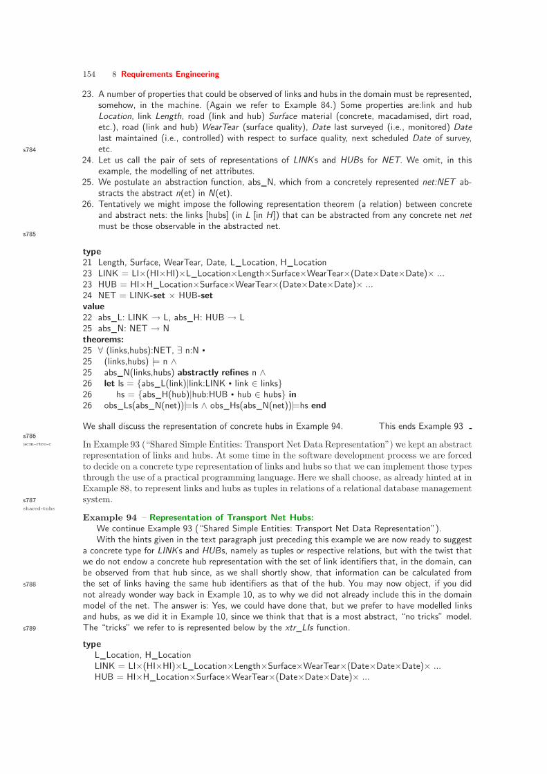
154 8 Requirements Engineering
23. A number of properties that could be observed of links and hubs in the domain must be represented,somehow, in the machine. (Again we refer to Example 84.) Some properties are:link and hubLocation, link Length, road (link and hub) Surface material (concrete, macadamised, dirt road,etc.), road (link and hub) WearTear (surface quality), Date last surveyed (i.e., monitored) Datelast maintained (i.e., controlled) with respect to surface quality, next scheduled Date of survey,etc.s784
24. Let us call the pair of sets of representations of LINK s and HUBs for NET. We omit, in thisexample, the modelling of net attributes.
25. We postulate an abstraction function, abs N, which from a concretely represented net:NET ab-stracts the abstract n(et) in N(et).
26. Tentatively we might impose the following representation theorem (a relation) between concreteand abstract nets: the links [hubs] (in L [in H ]) that can be abstracted from any concrete net netmust be those observable in the abstracted net.
s785
type21 Length, Surface, WearTear, Date, L Location, H Location23 LINK = LI×(HI×HI)×L Location×Length×Surface×WearTear×(Date×Date×Date)× ...23 HUB = HI×H Location×Surface×WearTear×(Date×Date×Date)× ...24 NET = LINK-set × HUB-setvalue22 abs L: LINK → L, abs H: HUB → L25 abs N: NET → Ntheorems:25 ∀ (links,hubs):NET, ∃ n:N •
25 (links,hubs) |= n ∧25 abs N(links,hubs) abstractly refines n ∧26 let ls = abs L(link)|link:LINK • link ∈ links26 hs = abs H(hub)|hub:HUB • hub ∈ hubs in26 obs Ls(abs N(net))|=ls ∧ obs Hs(abs N(net))|=hs end
We shall discuss the representation of concrete hubs in Example 94. This ends Example 93s786acm-rtre-c In Example 93 (“Shared Simple Entities: Transport Net Data Representation”) we kept an abstract
representation of links and hubs. At some time in the software development process we are forcedto decide on a concrete type representation of links and hubs so that we can implement those typesthrough the use of a practical programming language. Here we shall choose, as already hinted at inExample 88, to represent links and hubs as tuples in relations of a relational database managementsystem.s787
shared-tnhs
Example 94 – Representation of Transport Net Hubs:We continue Example 93 (“Shared Simple Entities: Transport Net Data Representation”).With the hints given in the text paragraph just preceding this example we are now ready to suggest
a concrete type for LINK s and HUBs, namely as tuples or respective relations, but with the twist thatwe do not endow a concrete hub representation with the set of link identifiers that, in the domain, canbe observed from that hub since, as we shall shortly show, that information can be calculated fromthe set of links having the same hub identifiers as that of the hub. You may now object, if you dids788
not already wonder way back in Example 10, as to why we did not already include this in the domainmodel of the net. The answer is: Yes, we could have done that, but we prefer to have modelled linksand hubs, as we did it in Example 10, since we think that that is a most abstract, “no tricks” model.The “tricks” we refer to is represented below by the xtr LIs function.s789
typeL Location, H LocationLINK = LI×(HI×HI)×L Location×Length×Surface×WearTear×(Date×Date×Date)× ...HUB = HI×H Location×Surface×WearTear×(Date×Date×Date)× ...

8.8 Interface Requirements 155
RDB = LINK-set × HUB-setvalue
xtr LIs: HUB → RDB → LI-setxtr LIs(hi,hl,s,wt,(ld,md,nd),...)(ls,hs) ≡li|li:LI•
∃ link:(li′,(hi′,hi′′),ll,lgt,s,wt,(d′,d′′,d′′′),...):LINK•
link ∈ ls ∧ (hi=hi′ ∨ hi=hi′′)
This ends Example 94s790acm-rtre-cThe requirements example that now follows to some extent deviate from the ideal of expressing
requirements: rather than expressing properties, the what, these requirements express an abstractdesign, the how. One might very well claim that the example that now follows really should bemoved to a section on Software Design since it can be said to be such an abstract design. Be that asit may, we have chosen to place the next example here, under shared entity data initialisation, asit illustrates that concept rather well. The point is that the more we include considerations of themachine the the more operational, that is, the less what the more how the interface requirementsbecomes.
s791 shared-tndi
Example 95 – Shared Simple Entities: Transport Net Data Initialisation: We continue Exam-ple 93 (“Shared Simple Entities: Transport Net Data Representation”). We now focus on the initiali-sation of simple entity data.
27. Input of representations of simple transport net entities, that is, representations of links and hubs,is by means of a software package, call it NetDataInput.
28. NetDataInput assumes a rather old-fashioned constellation of a graphic user interface (GUI),NetDataGUI, in-data and a conventional relational database NetDataRDB.
29. The NetDataRDB is here thought of as just consisting of two relations ls:LINKS and hs:HUBS. s792
30. Each relation consists of a set of LINK, respectively HUB “tupleisations” of links and hubs — which,to repeat, are representations of links and hubs .
31. When NetDataInput is invoked, the NetDataInput GUI shall open in a window with a click-able,simple either/or choice icon: Road Net or Rail Net.
32. Clicking one of these shall result in replacing the either/or window being replaced by a window forthe input of net units for the selected choice of net. s793
In the following we shall treat only the Road Net variant of this interface requirements.33. The Road Net (GUI) window has the following alternative click-able choice icons: link and hub.34. Clicking the Road Net link icon shall result in replacing the Road Net window being replaced by
a window for the input of representations of road links. Similarly for clicking the Road Net link
icon.In the following we shall treat only the Road Net link icon variant of this interface requirements.
s794
35. The Road Net link window has the following named fields:
• link identifier fill in
• hub identifier 1 fill in
• hub identifier 2 fill in
• link location fill in
• link surface fill in
• link wear & tear fill in
• a triple of link dates:⋆ last survey fill in
⋆ last maintenance fill in
⋆ next survey fill in
• et cetera.• submit
Each field, except for the submit icon, consists of a name part and an input, fill in , part. (Inthe formalisation below the type names “cover” both parts.) The system shall assign unique linkidentifiers, i.e., “fill-in” the link identifier automatically. s795
36. Clicking the submit icon shall result in the following checks:

156 8 Requirements Engineering
• The composite in-data, keyed into the input parts of the Road Net link window fields arevetted:⋆ Is the link identifier already defined ?⋆ Do the location co-ordinates conflict with earlier input ?⋆ Are the dates in an appropriate chronological order ?⋆ Et cetera.
• If checks are OK, then the following actions are performed:⋆ The NetDataRDB link relation is updated to reflect the new link tuple.⋆ The Road Net system then reverts to the Road Net link window, allowing, however, the
input staff to select the alternative (i) Road Net hub window, or (ii) to request a partialor full vetting of the state of the NetDataRDB link and hub relations, (iii) or to concludethe input on net data.
s796
Here we stop our ‘abstract’ narrative of interface requirements for data (i.e., simple entity) initialisation.We next rough-sketch the beginnings of a formalisation.
Rail / Road Link / Hub
Road Net Link
Link Id:Hub 1: Location:
Wear&Tear:Last SurveyLast MaintenanceNext Survey
Surface:
Dates:
Hub 2:
Net Initialisation Road Net
...vet concluderoad net hub ...
Fig. 8.2. Three snapshots of NetDataInput
s797
type27 NDI29 RDB = Links × Hubs30 Links = LINK-set30 Hubs = HUB-set31 GUI == EitherOrW | RoadNetW | RailNetW31 EitherOrW == roadnet | railnet33 RoadNetW == link | hub35 LINK = LI×(HI×HI)×L Location×Surface×WearTear×(Date×Date×Date)× ...35 HUB = HI×H Location×Surface×WearTear×(Date×Date×Date)× ...
Response == ok | (not ok × Error Msg)Error Msg
value28 obs GUI: NDI → GUI, obs RDB: NDI → RDB32 select RoadOrRail: GUI → GUI34 select Link or Hub: GUI → GUI36 submit Link input: GUI → GUI × Response
We leave it to the reader to complete the interface requirements for shared simple entity initialisation.A similar set of interface requirements can be established for for shared simple entity refreshment.
This ends Example 95

8.8 Interface Requirements 157
8.8.3 Shared Operation Requirements s798
acm-rtre-c
Definition 73 – Shared Operation: By a shared operation we understand an operation of thedomain that can only be partially ‘executed’ by the machine — with the remaining operation partsbeing “executed” by a human or some “gadget” of the domain “outside” of our concern.
We start by giving a consolidated domain description of a fragment of a financial servicesindustry, in other words: Example 96 is not a requirements prescription. But it will be the basisfor a shared operations interface requirements prescription. s799
pfm-shrd-tops
Example 96 – Shared Operations: Personal Financial Transactions: With the advent of theInternet,i.e., computing and communications, and with the merging of in-numerous functionalities ofthe financial service sector, we are witnessing the ability of some clients of the financial service industryto handle most of their transactions “themselves”.
In the first part, Items 37–45 of this example, we rough-sketch the state and the signatures of someof the client operations of a financial service industry. In the second part, Items 50–62, we rough sketchclient states and behaviours. s800
37. The financial service industry includes one or mare banking and securities instrument tradingservices.a) Banks are uniquely identified (BId).b) Banks offer accounts:
i. a client may have one or more demand/deposit accounts andii. one or more mortgage accounts, identified by account numbers;
accounts, in this simplified example, holds a balance of (deposited or mortgaged) money.c) Two or more clients may share accounts and bank registers correlate client names (C ) to
account and (A) mortage (M) account numbers.d) We do not describe bank identifiers, client names, demand/deposit account numbers, mortgage
account numbers,s801
type37 Banks, SecTrad37a Banks = BId →m Bank37b Bank = Registers × Accounts × Mortgages × ...37(b)i Accounts = A →m Account37(b)ii Mortgages = M →m Mortgage37c Registers = C →m (A|M)-set37d C, A, BId, Account, Mortgage, Account, Mortgage, OrdNr
s802
38. Bank clientsa) open account andb) close (demand/deposit and mortgage) accounts,c) deposit money into accounts,d) transfer money to (possibly other client) accounts (possibly in other banks and to/from security
traders’ bank accounts — the latter reference also to buy and sell offer order numbers, OrdNr),and
e) withdraw (cash) money (say, through an ATM).39. Client supplied arguments to and40. responses from these banking operations are also not further described.
s803
value38a openacct: Arg∗ → Banks → Banks × Response38b closeacct: Arg∗ → Banks → Banks × Response38c deposit: Arg∗ → Banks → Banks × Response

158 8 Requirements Engineering
38d transfer: Arg∗ → Banks → Banks × Response38e withdraw: Arg∗ → Banks → Banks × Responsetype39 Arg = BId | C | A | M | OrdNr | Amount | Cash | Date | Time40 Response = (A | M | Cash | ... | Date | Time)-set
s804
41. A securities exchange keeps track of buy and sell offers, of suspended such offerings and of trans-acted trading.
42. Basic concepts of trading, apart from buying, selling, suspension and concluded trading, area) securities instrument identifications (SId);b) quantities offered for selling or buying, or traded (Quant);c) the order numbers of placed offers (OrdNr),d) prices (Price),e) dates (Date) andf) times (Time).
type41 SecTrad = BuyOfrs × SellOfrs × Suspension × Tradings42 SId, Quant, OrdNr, Price, Date, Time, ...
s805
43. Securities trading allows clientsa) to place buy andb) sell offers,giving their client and bank identification, their bank demand/deposit account number (from whichto withdraw [i.e., demand], resp. into which to deposit) buying or selling prices), the securitiesinstrument [e.g., stock] identifier, quantity to be bought or sold, the high, respectively the lowprice acceptable, and the last date of the offer.
44. Clients may inquire as to the trading status of their offer.45. We can therefore think of the following kinds of client transaction “codes” (Cmd): omkt (observe
the market), open (some kind of bank or securities trading account: demand/deposit, mortgage,trading, etc.), deposit, withdraw, transfer, close, buy offer, sell offer, inquire, et cetera.
s806
value43a int buyofr: Arg∗ → SecTrad → SecTrad × Response43b int sellofr: Arg∗ → SecTrad → SecTrad × Response44 trading: SecTrad → SecTrad × Response
type45 Cmd == obsmkt|analmkt|openacct|deposit|withdraw|transfer|closeacct|...|buyofr|sellofr|trading|...
s807We can, finally, suggest crucial components of the securities exchange state:
46. BuyOfrs map client names, C, into (client) bank identifiers, BId, and client account numbers, A,which then map into OrdNrs, which (then again) map into a quadruple of securities instrumentidentifications, SId,Quantity of instrument to be bought, the preferred lowest Price and the Dateof placement or order.
47. SellOfrs have same components as buy offers — but now the Price designate a highest price.48. Suspensions just list order number and date and time of suspension.49. Tradings list pertinent information.
type46 BuyOfr = OrdNr →m (C × BId × A) →m (SId × Quant × Price × Date)47 SellOfr = OrdNr →m (C × BId × A) →m (SId × Quant × Price × Date)48 Suspension = OrdNr →m (C × Date × Time)49 Tradings = OrdNr →m SId × Quant × Price × (C×Bid×A×(Date×Time))

8.8 Interface Requirements 159
s808We now rough-sketch a concept of ‘personal finance management’ operations. It is in this part, notthe first, that this example reveals that it is an example of an operation that is shared between thedomain and the machine. We maintain, however, that the example is still that of a domain description.The operation is that of a client managing own, personal finances. This ‘personal finance management’ s809
operation is a composite operation. It is a sequence of ”one-step” operations, each operation being abanking or a securities trading. (For simplicity, but without any loss of generality, we limit the exampleto just these two sets of operations.) Each such operation results in a date- and time-stamped response(Item 40 on page 157). Each response is studied by the client. The client may then decide to proceedwith further ‘one-step’ operations or end this sequence “at this time” — allowing, of course, the clientto resume ‘personal finance management’ at a later ‘personal finance management session’. s810
40. Each of the banking and securities instrument operations result in a response.50. This response becomes part of the client’s ‘finance management’ state, ΠΦΣ.51. We refer to the global financial service industry state as Ω.
Besides the banks and securities trading, the global financial service industry state (ω:Ω)is thought of as including all those aspects of the clients of this industry which affectsand/or reflects the financial situation.
52. A ‘personal finance management (pfm) session’ is now a conditional iteration (formula Line 56below) of personal finance management operations. s811
53. A client can always observe the dated and timed responses received as a result of past personalf inance management operations.
54. An iteration of ‘personal finance management’ starts with the client analysing (ω anal mkt) themarket based on past responses;
55. followed by an analysis (cli anal mkt) of the personal financial situation based on the marketresponse.
56. If the analysis advises some ‘personal finance management’57. then the client inquires, what to do, past responses and as to which transaction, cmd, and with
which arguments, argl, such a transaction should be performed.This operation, what to do, is not computable. It is an operation performed basically bythe client. s812
58. The client then performs (Int Cmd) this (i.e., the cmd) transaction. The transaction usuallytransforms the finance industry state (ω) into a next state (ω′) and always yields a date- and
59. Once the transaction has been concluded the client reverts to the ‘personal finance management(pfm) session’ with an updated “past responses” (merge pfm) and in the new global state, ω′.
60. Else, that is, if the analysis “advises” no transactions, the ‘personal finance management’ state,πφσ and the global financial state, ω, is left unchanged and the (i.e., this) session ends.
61. To perform a transaction depends on which kind of transaction, cmd, has been advised.62. We leave the interpretation of Int Cmd to the reader.
π The lines, below, marked π designate actions that are performed by the client or jointly betweenthe client and the financial system (designated by an ω or ω′ argument).
s813
type50–51 ΠΦΣ, Ω53 Responses = (Date×Time) →m Response45 Cmd == obsmkt|analmkt|openacct|deposit|withdraw|transfer|closeacct|...|buyofr|sellofr|trading|...value53 obs Responses: ΠΦΣ → Responses52 pfm session: ΠΦΣ → Ω → Ω × ΠΦΣ52 pfm session(πφσ)(ω) ≡53π let past responses = obs Responses(πφσ) in54π let ω response = ω anal mkt(past responses)(ω) in55π let πφσ response = cli anal mkt(response)(πφσ) in56π if advice pfm action(πφσ response)

160 8 Requirements Engineering
57π then let (cmd,argl) = what to do(πφσ response)(ω) in58 let (response,ω′) = Int Cmd(cmd,argl)(ω) in59π pfm session(merge pfm(response,date,time)(πφσ))(ω′) end end end60 else (ω,πφσ) end end end54 ω anal mkt: Responses → Ω → Response55π cli anal mkt: Response → ΠΦΣ → Response56 advice pfm action: Response → Bool57π what to do: Responses → Ω → Cmd × Arg∗
59π merge pfm: Responses → ΠΦΣ → Ω → Ω × ΠΦΣ
s814
61. To perform a transaction depends on which kind of transaction, cmd, has been advised.63. A case distinction is made between the very many kinds of transactions (listed in Item 45).64. The obs mkt and anal pfm operations do not change the state of the financial industry.
We think of these operations as not being computable functions. Rather we think of themas a more-or-less “informed” study, by the client of the market of financial instrumentsincluding the status of those enterprises whose stocks are traded.
65. The argument l ist of the open transaction indicates which kind of account is to be established(demand/deposit, mortgage, etc.).
66. The argument l ist of the buy of fer transaction indicates which kind of securities (stocks, oil,metals, or other commodities) is sought, in which quantity, at which price level, up till which date,et cetera.
s815
value61 Int Cmd: (Cmd × Arg∗) → Ω → Ω × Response61 Int Cmd(cmd,argl)(ω) ≡63 case cmd of64π obsmkt → (ω,eval obs mkt(argl)(ω)),64π analmkt → (ω,ω anal mkt(argl)(ω)),
...65π openacct → int open acct(argl)(ω),
...66π buyofr → int buyofr(argl)(ω),
...63 end
64π eval obs mkt: Arg∗ → Ω → Response64π ω anal mkt: Arg∗ → Ω → Response65 int open acct: Arg∗ → Ω → Ω × Response66 int buyofr: Arg∗ → Ω → Ω × Response
This ends Example 96s816acm-rtre-c The reader may well ask: What in Example 96 illustrates the shared operations interface require-
ments ? We have already indicated part of the answer to this question by the π annotations. Why isthis a reasonable question ? It is a reasonable question because we have not made that abundantlyclear. That is, we have not discussed the placement of π annotations in much detail. Example 96could really be construed as a domain description based in the intrinsics, support technology,management and organisation and human behaviour regime.
8.8.4 Shared Event Requirements s817
acm-rtre-c
Definition 74 – Shared Event: By a shared event we understand an event of the domain thatmust be brought to the attention of the machine.

8.8 Interface Requirements 161
We defer the exemplification of shared events till our treatment of ‘shared behaviour’. InSect. 8.8.5 we exemplify ‘shared behaviours’. The ‘step of development’, from the specification ofExample 96 (Shared Operations) to the specification of Example 97 (Shared Behaviours) is not aformal refinement: but it can be made into such a formally verifiable refinement. So we pose thatas a relevant MSc Thesis topic.
8.8.5 Shared Behaviour Requirements s818
Definition 75 – Shared Behaviour: By a shared behaviours we understand a behaviour of thedomain that can only be partially ‘processed’ by the machine — with the remaining behaviour beingprovided by humans or some “gadgets” of the domain,“outside” of our concern.
s819pfm-shrd-bhvs
Example 97 – Shared Behaviours: Personal Financial Transactions:
67. There is an index set, CI, of clients.68. For each client there is an “own”69. ‘personal finance management’ state πφσci : ΠΦΣ (cf. 50 on page 159).70. The finance industry “grand state” ω : Ω is as before (cf. Item and formula line 51 on page 159).71. The system consists of
a) an indexed set of client behavioursb) and one finance industry “grand state” behaviour omega.
72. We model communications between clients and the financial industry to occur over client-industrychannels.
73. We model communications over these channels as being of type M. M will be “revealed” as we goon.
s820
type67 CI68 ΠΦΣs = CI →m ΠΦΣ69 ΠΦΣ70 Ω = Banks × SecTrad × ...value67 cis:CI-set68 πφσs:ΠΦΣs70 ω:Ω71 system: Unit → Unit71 system() ≡71a ‖ client(ci)(πφσs(ci))|ci:CI•ci ∈ cis71b ‖ omega(ω)channel72 c ω ch[ ci ]|ci:CI•ci ∈ cis Mtype73 M
s821Let us first consider the issue of events. First the events arise in “the market”, here symbolised withthe global state ω : Ω.
74. The omega(ω) behaviour and the client(ci)(πφσs(ci)) behaviours, for all clients, are cyclic —expressed through ‘tail recursion’ over possibly updated states.
75. To model events we let the omega(ω) behaviour alternate between eithera) inquiring its state as to unusual situations in, the status status of, “the market”, and,b) if so, inform an arbitrary subsets of clients of such “events” andc) continuing in an unchanged global financial system state
or
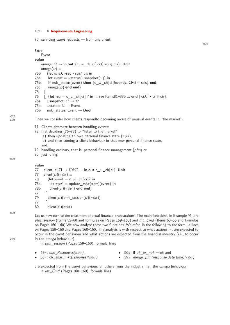
162 8 Requirements Engineering
76. servicing client requests — from any client.s822
typeEvent
valueomega: Ω → in,out c ω ch[ ci ]|ci:CI•ci ∈ cis Unitomega(ω) ≡
75b (let scis:CI-set • scis⊆cis in75a let event = ωstatus(ωsnapshot(ω)) in75b if nok status(event) then c ω ch[ ci ]!event|ci:CI•ci ∈ scis end;75c omega(ω) end end)75 ⌈⌉76 ⌈⌉⌊⌋ let req = c ω ch[ ci ] ? in ... see Items81–88b ... end | ci:CI • ci ∈ cis75a ωsnapshot: Ω → Ω75a ωstatus: Ω → Event75b nok status: Event → Bool
s823Then we consider how clients respondto becoming aware of unusual events in “the market”.s824
77. Clients alternate between handling events:78. first deciding (76–78) to “listen to the market”,
a) then updating an own personal finance state (πφσ),b) and then coming a client behaviour in that new personal finance state,and
79. handling ordinary, that is, personal finance management (pfm) or80. just idling.
s825
value77 client: ci:CI → ΠΦΣ → in,out c ω ch[ ci ] Unit77 client(ci)(πφσ) ≡78 (let event = c ω ch[ ci ]? in78a let πφσ′ = update πφσ(πφσ)(event) in78b client(ci)(πφσ′) end end)77 ⌈⌉79 client(ci)(pfm session(ci)(πφσ))77 ⌈⌉80 client(ci)(πφσ)
s826Let us now turn to the treatment of usual financial transactions. The main functions, in Example 96, arepfm session (Items 52–60 and formulas on Pages 159–160) and Int Cmd (Items 63–66 and formulason Pages 160–160) We now analyse these two functions. We refer, in the following to the formula lineson Pages 159–160 and Pages 160–160. The analysis is with respect to what actions, π, are expected tooccur in the client behaviour and what actions are expected from the financial industry (i.e., to occurin the omega behaviour).s827
In pfm session (Pages 159–160), formula lines
• 53π: obs Responses(πφσ),• 55π: cli anal mkt(response)(πφσ),
• 56π: if ok or nok = ok and• 59π: merge pfm(response,date,time)(πφσ)
are expected from the client behaviour, all others from the industry, i.e., the omega behaviour.In Int Cmd (Pages 160–160), formula lines

8.8 Interface Requirements 163
• 64π: eval obs mkt(argl)(ω),• 64π: ω anal mkt(argl)(ω),• 65π: int open acct(argl)(ω),
• . . . ,• 66π: int buyofr(argl)(ω),• . . . ,
are expected from the client behaviour. s828
Of the functions itemised above, the
81. (54π) ω anal mkt(past responses)(ω),82. (64π) eval obs mkt(ω),83. (65π) int open acct(argl)(ω),
84. . . . ,85. (66π) int buyofr(argl)(ω),86. . . . ,
functions — as invoked by the client, in the pfm session and the Int Cmd behaviours — requireaccess to the global financial service industry state ω.
The idea is now, for the client, in its Int Cmd (see Formula lines 61.0 onwards [Page 164]) tocommunicate these functions, as function named argument lists, cf. Formula lines 81–86 below.
s829
typeFCT == Anal mkt|Obs mkt|...|Open aact|...|Buy Ofr|...
81 Anal mkt = mkAnalMkt(argl:Arg∗)82 Obs mkt = mkObsMkt(argl:Arg∗)83 Open acct = mkOpenAcct(argl:Arg∗)84 ...85 Buy Ofr = mkBuyOfr(argl:Arg∗)86 ...channel72 c ω ch[ ci ]|ci:CI•ci ∈ cis: Event | FCT | Response
s830
87. The omega behaviour thus alternatesa) between accepting and responding to either of the many forms of functions, FCTb) or generating event notifications.
88. If the omega behaviour of its own will, that is, internally non-deterministically chooses to accept aclient initiate request it externally non-deterministically chooses which client request to serve.a) The omega behaviour deciphers the request;b) applies the communicated function to (possibly communicated arguments) and the ω”grand
state”; and communicates the result back to the chosen client.
s831
valueomega: Ω → in,out c ω ch[ ci ]|ci:CI•ci ∈ cis Unitomega(ω) ≡
87b (let scis:CI-set • scis⊆cis in87b let event = ωstatus(ωsnapshot(ω)) in87b if nok status(event) then c ω ch[ ci ]!event|ci:CI•ci ∈ scis end;87b omega(ω) end end)87 ⌈⌉88 ⌈⌉⌊⌋ let req = c ω ch[ ci ] ? in88a case req of87a mkObsMkt(argl) → c ω ch[ ci ] ! eval obs mkt(argl)(ω) ; omega(ω),87a mkAnalMkt(argl) → c ω ch[ ci ] ! ω anal mkt(argl)(ω) ; omega(ω),87a mkOpenAcct(argl) →88a let (ω′,res) = int open acct(argl)(ω) in c ω ch[ ci ] ! res ; omega(ω′) end,

164 8 Requirements Engineering
87a ...87a mkBuyOfr(argl) →88a let (ω′,res) = int buyofr(argl)(ω) in c ω ch[ ci ] ! res ; omega(ω′) end,87a ...88a end end | ci:CI • ci ∈ cis
Some auxiliary functions:s832
value64π eval obs mkt: Arg∗ → Ω → Response64π ω anal mkt: Arg∗ → Ω → Response65 int open acct: Arg∗ → Ω → Ω × Response66 int buyofr: Arg∗ → Ω → Ω × Response
There is only minor changes, marked√
, to pfm session: (52) an additional argument, ci:CI and (58)an additional argument, (ci) to Int Cmd(ci)(cmd,argl).s833
value52√
pfm session: ci:CI → ΠΦΣ → in,out ωch ΠΦΣ52√
pfm session(ci)(πφσ) ≡53 let past responses = obs Responses(πφσ) in54 let response = ωch[ ci ]!mkObsMkt(past responses); ωch[ ci ] ? in55 let response = analyse pfm(past responses)(πφσ) in56 if advice pfm action(response)57 then (let (cmd,argl) = what pfm to do(response) in58√
let response = Int Cmd(ci)(cmd,argl) in59√
pfm session(ci)(merge pfm(response)(πφσ)) end end) end60 else πφσ end end end
56 advice pfm action: Response → Bool55 analyse pfm: Responses → (|ok||Event) → |ok|nok|
Similarly the changes to Int Cmd are obvious and marked, as before, with .i, i = 0, 1, 2, 3:s834
value61.0 Int Cmd: ci:CI × (Cmd × Arg∗) → in,out ωch Response61 Int Cmd(ci)(cmd,argl) ≡61 case cmd of61.2 obsmkt → ωch[ ci ]!mkObsMkt(argl) ; ωch[ ci ]?61.2 analpfm → ωch[ ci ]!mkAnalMkt(argl) ; ωch[ ci ]?61 ...61.2 openacct → ωch[ ci ]!mkOpenAcct(argl) ; ωch[ ci ]?61 ...61.3 buyofr → ωch[ ci ]!mkBuyOfr(argl) ; ωch[ ci ]?61 ...61 end
This ends Example 97
Discussion s835
acm-rtre-c
to be written

8.9 Machine Requirements 165
8.9 Machine Requirements s836
acm-rtre-d
Definition 76 – Machine Requirements: By machine requirements we understand those re-quirements that can be expressed solely in terms of (or with prime reference to) machine concepts
8.9.1 An Enumeration of Machine Requirements Issues s837
There are many separable machine requirements. To find one’s way around all these separablemachine requirements we shall start by enumerating the very many that we shall overview.
s838
1. Performance Requirements from Page 166
a) Storage Requirements from Page 167b) Machine Cycle Requirements from Page 167c) Other Resource Consumption Requirements from Page 167
2. Dependability Requirements from Page 167
a) Accesability Requirements from Page 168b) Availability Requirements from Page 169c) Integrity Requirements from Page 169d) Reliability Requirements from Page 169e) Safety Requirements from Page 169f) Security Requirements from Page 170
s839
3. Maintenance Requirements from Page 170
a) Adaptive Maintenance Requirements from Page 171b) Corrective Maintenance Requirements from Page 171c) Perfective Maintenance Requirements from Page 171d) Preventive Maintenance Requirements from Page 171
4. Platform Requirements from Page 172
a) Development Platform Requirements from Page 172b) Execution Platform Requirements from Page 172c) Maintenance Platform Requirements from Page 172d) Demonstration Platform Requirements from Page 172
5. Documentation Requirements from Page 173
8.9.2 Performance Requirements s840
Definition 77 – Performance Requirements: By performance requirements we understand ma-chine requirements that prescribe storage consumption, (execution, access, etc.) time consumption,as well as consumption of any other machine resource: number of CPU units (incl. their quanti-tative characteristics such as cost, etc.), number of printers, displays, etc., terminals (incl. theirquantitative characteristics), number of “other”, ancillary software packages (incl. their quantita-tive characteristics), of data communication bandwidth, etcetera.
s841
Pragmatically speaking, performance requirements translate into financial resources spent, or tobe spent.
Example 98 – Timetable System Performance: We continue Example 86 on page 149. Themachine shall serve 1000 users and 1 staff simultaneously. Average response time shall be at most 1.5seconds, when the system is fully utilised. This ends Example 98

166 8 Requirements Engineering
General s842
Till now we may have expressed certain (functions and) behaviours as generic (functions and)behaviours. From now on we may have to “split” a specified behaviour into an indexed family ofbehaviours, all “near identical” save for the unique index. And we may have to separate out, as aspecial behaviour, (those of) shared entities.
s843
Example 99 – Timetable System Users and Staff: We continue Example 83 on page 146 andExample 98 on the previous page. In Example 83 the sharing of the timetable between users and staffwas expressed parametrically.
system(tt) ≡ client(tt) ⌈⌉ staff(tt)
client: TT → Unitclient(tt) ≡ let q:Query in let v =Mq(q)(tt) in system(tt) end end
staff: TT → Unitstaff(tt) ≡
let u:Update in let (r,tt′) =Mu(u)(tt) in system(tt′) end end
s844We now factor the timetable entity out as a separate behaviour, accessible, via indexed communications,i.e., channels, by a family of client behaviours and the staff behaviour.
typeCIdx /∗ Index set of, say 1000 terminals ∗/
channel ct[ i ]:QU,tc[ i ]:VAL | i:CIdx st:UP,ts:RES
valuesystem: TT → Unitsystem(tt) ≡ time table(tt) ‖ (‖ client(i)|i:CIdx) ‖ staff()
s845
client: i:CIdx → out ct[ i ] in tc[ i ] Unitclient(i) ≡ let qc:Query in ct[ i ]!Mq(qc) end tc[ i ]?;client(i)
staff: Unit → out st in ts Unitstaff() ≡ let uc:Update in st!Mu(uc) end let res = ts? in staff() end
time table: TT → in ct[ i ]|i:CIdx,st out tc[ i ]|i:CIdx,ts Unittime table(tt) ≡⌈⌉⌊⌋ let qf = ct[ i ]? in tc[ i ]!qf(tt) end | i:CIdx⌈⌉⌊⌋ let uf = st? in let (tt′,r)=uf(tt) in ts!r; time table(tt′) end end
s846Please observe the “shift” from using ⌈⌉ in system earlier in this example to ⌈⌉⌊⌋ just above. The formerexpresses nondeterministic internal choice. The latter expresses nondeterministic external choice. Thechange can be justified as follows: The former, the nondeterministic internal choice, was “between”two expressions which express no external possibility of influencing the choice. The latter, the non-deterministic external choice, is “between” two expressions where both express the possibility of anexternal input, i.e., a choice. The latter is thus acceptable as an implementation of the former.
This ends Example 99s847
The next example, Example 100, continues the performance requirements expressed just above.Those two requirements could have been put in one phrase, i.e., as one prescription unit. But weprefer to separate them, as they pertain to different kinds (types, categories) of resources: terminal+ data communication equipment facilities versus time and space.s848

8.9 Machine Requirements 167
Example 100 – Storage and Speed for n-Transfer Travel Inquiries: We continue Example 86on page 149. When performing the n-Transfer Travel Inquiry (rough sketch) prescribed above, the first— of an expected many — result shall be communicated back to the inquirer in less than 5 secondsafter the inquiry has been submitted, and, at no time during the calculation of the “next” results mustthe storage buffer needed to calculate these exceed around 100,000 bytes.
Storage Requirements s849
Machine Cycle Requirements s850
Other Resource Consumption s851
8.9.3 Dependability Requirements s852
To properly define the concept of dependability we need first introduce and define the conceptsof failure, error, and fault.
s853
Definition 78 – Failure: A machine failure occurs when the delivered service deviates fromfulfilling the machine function, the latter being what the machine is aimed at [122].
s854
Definition 79 – Error: An error is that part of a machine state which is liable to lead tosubsequent failure. An error affecting the service is an indication that a failure occurs or hasoccurred [122].
s855
Definition 80 – Fault: The adjudged (i.e., the ‘so-judged’) or hypothesised cause of an error isa fault [122].
The term hazard is here taken to mean the same as the term fault.One should read the phrase: “adjudged or hypothesised cause” carefully: In order to avoid an
unending trace backward as to the cause,10 we stop at the cause which is intended to be preventedor tolerated.
s856
Definition 81 – Machine Service: The service delivered by a machine is its behaviour as it isperceptible by its user(s), where a user is a human, another machine or a(nother) system whichinteracts with it [122].
Definition 82 – Dependability: Dependability is defined as the property of a machine such thatreliance can justifiably be placed on the service it delivers [122].
s857
We continue, less formally, by characterising the above defined concepts [122]. “A given machine,operating in some particular environment (a wider system), may fail in the sense that some othermachine (or system) makes, or could in principle have made, a judgement that the activity orinactivity of the given machine constitutes a failure”.
The concept of dependability can be simply defined as “the quality or the characteristic ofbeing dependable”, where the adjective ‘dependable’ is attributed to a machine whose failures arejudged sufficiently rare or insignificant.
Impairments to dependability are the unavoidably expectable circumstances causing or result-ing from “undependability”: faults, errors and failures. Means for dependability are the techniquesenabling one to provide the ability to deliver a service on which reliance can be placed, and to reachconfidence in this ability. Attributes of dependability enable the properties which are expected from

168 8 Requirements Engineering
the system to be expressed, and allow the machine quality resulting from the impairments andthe means opposing them to be assessed. s858
Having already discussed the “threats” aspect, we shall therefore discuss the “means” aspectof the dependability tree.
• Attributes:⋆ Accessibility⋆ Availability⋆ Integrity⋆ Reliability⋆ Safety⋆ Securitys859
• Means:⋆ Procurement· Fault prevention· Fault tolerance
⋆ Validation· Fault removal· Fault forecasting
• Threats:⋆ Faults⋆ Errors⋆ Failures
s860
Despite all the principles, techniques and tools aimed at fault prevention, faults are created. Hencethe need for fault removal. Fault removal is itself imperfect. Hence the need for fault forecasting.Our increasing dependence on computing systems in the end brings in the need for fault tolerance.s861
Definition 83 – Dependability Attribute: By a dependability attribute we shall mean either oneof the following: accessibility, availability, integrity, reliability, robustness, safety and security. Thats862
is, a machine is dependable if it satisfies some degree of “mixture” of being accessible, available,having integrity, and being reliable, safe and secure.
The crucial term above is “satisfies”. The issue is: To what “degree”? As we shall see — in a latersection — to cope properly with dependability requirements and their resolution requires thatwe deploy mathematical formulation techniques, including analysis and simulation, from statistics(stochastics, etc.).
In the next seven subsections we shall characterise the dependability attributes further. Indoing so we have found it useful to consult [98].
Accesability Requirements s863
Usually a desired, i.e., the required, computing system, i.e., the machine, will be used by manyusers — over “near-identical” time intervals. Their being granted access to computing time isusually specified, at an abstract level, as being determined by some internal nondeterministicchoice, that is: essentially by “tossing a coin”! If such internal nondeterminism was carried over,into an implementation, some “coin tossers” might never get access to the machine.s864
Definition 84 – Accessibility: A system being accessible — in the context of a machine beingdependable — means that some form of “fairness” is achieved in guaranteeing users “equal” accessto machine resources, notably computing time (and what derives from that).
s865
10An example: “The reason the computer went down was the current supply did not deliver sufficientvoltage, and the reason for the drop in voltage was that a transformer station was overheated, and thereason for the overheating was a short circuit in a plant nearby, and the reason for the short circuit in theplant was that . . . , etc.”

8.9 Machine Requirements 169
Example 101 – Timetable Accessibility: Based on Examples 83 on page 146 and 86 on page 149,we can express: The timetable (system) shall be “inquirable” by any number of users, and shall beupdate-able by a few, so authorised, airline staff. At any time it is expected that up towards a thousandusers are directing queries at the timetable (system). And at regular times, say at midnights betweenSaturdays and Sundays, airline staff are making updates to the timetable (system). No matter howmany users are “on line” with the timetable (system), each user shall be given the appearance thatthat user has exclusive access to the timetable (system).
Availability Requirements s866
Usually a desired, i.e., the required, computing system, i.e., the machine, will be used by manyusers — over “near-identical” time intervals. Once a user has been granted access to machineresources, usually computing time, that user’s computation may effectively make the machineunavailable to other users — by “going on and on and on”! s867
Definition 85 – Availability: By availability — in the context of a machine being dependable —we mean its readiness for usage. That is, that some form of “guaranteed percentage of computingtime” per time interval (or percentage of some other computing resource consumption) is achieved— hence some form of “time slicing” is to be effected.
s868
Example 102 – Timetable Availability: We continue Examples 83 on page 146, 86 on page 149and 101: No matter which query composition any number of (up to a thousand) users are directingat the timetable (system), each such user shall be given a reasonable amount of compute time permaximum of three seconds, so as to give the psychological appearance that each user — in principle —“possesses” the timetable (system). If the timetable system can predict that this will not be possible,then the system shall so advise all (relevant) users.
Integrity Requirements s869
Definition 86 – Integrity: A system has integrity, in the context of a machine being dependable,if it is and remains unimpaired, i.e., has no faults, errors and failures, and remains so even in thesituations where the environment of the machine has faults, errors and failures.
Integrity seems to be a highest form of dependability, i.e., a machine having integrity is 100%dependable! The machine is sound and is incorruptible.
Reliability Requirements s870
Definition 87 – Reliability: A system being reliable, in the context of a machine being depend-able, means some measure of continuous correct service, that is, measure of time to failure.
Example 103 – Timetable Reliability: Mean time between failures shall be at least 30 days, anddowntime due to failure (i.e., an availability requirements) shall, for 90% of such cases, be less than 2hours.
Safety Requirements s871
Definition 88 – Safety: By safety — in the context of a machine being dependable — we meansome measure of continuous delivery of service of either correct service, or incorrect service afterbenign failure, that is: Measure of time to catastrophic failure.
Example 104 – Timetable Safety: Mean time between failures whose resulting downtime is morethan 4 hours shall be at least 120 days.

170 8 Requirements Engineering
Security Requirements s872
We shall take a rather limited view of security. We are not including any consideration of securityagainst brute-force terrorist attacks. We consider that an issue properly outside the realm ofsoftware engineering.
Security, then, in our limited view, requires a notion of authorised user, with authorised usersbeing fine-grained authorised to access only a well-defined subset of system resources (data, func-tions, etc.). An un-authorised user (for a resource) is anyone who is not authorised access to thatresource.
A terrorist, posing as a user, should normally fail the authorisation criterion. A terrorist, posingas a brute-force user, is here assumed to be able to capture, somehow, some authorisation status.We refrain from elaborating on how a terrorist might gain such status (keys, passwords, etc.)!s873
Definition 89 – Security: A system being secure — in the context of a machine being dependable— means that an un-authorised user, after believing that he or she has had access to a requestedsystem resource: (i) cannot find out what the system resource is doing, (ii) cannot find out how thesystem resource is working and (iii) does not know that he/she does not know! That is, preventionof un-authorised access to computing and/or handling of information (i.e., data).
s874
The characterisation of security is rather abstract. As such it is really no good as an a priori designguide. That is, the characterisation gives no hints as how to implement a secure system. But, oncea system is implemented, and claimed secure, the characterisation is useful as a guide on how totest for security!s875
Example 105 – Timetable Security: We continue Examples 83 on page 146, 86 on page 149, 101on the preceding page, and 102 on the previous page. Timetable users can be any airline client loggingin as a user, and such (logged-in) users may inquire the timetable. The timetable machine shall besecure against timetable updates from any user. Airline staff shall be authorised to both update andinquire, in a same session.
s876
Example 106 – Hospital Information System Security: General access to (including copyingrights of) specially designated parts of a(ny) hospital patient’s medical journals is granted, in principle,only to correspondingly specially designated hospital staff. In certain forms of (otherwise well-defined)emergency situations any hospital paramedic, nurse or medical doctor may “hit a panic button”, gettingaccess to a hospital patient’s medical journal, but with only viewing, not copying rights. Such incidentsshall be duly and properly recorded and reported, such that proper post-processing (i.e., evaluation) ofsuch “panic button” accesses can take take place.
Robustness Requirements s877
Definition 90 – Robustness: A system is robust — in the context of dependability — if it retainsits attributes after failure, and after maintenance.
Thus a robust system is “stable” across failures and “across” possibly intervening “repairs” and“across” other forms of maintenance.
• • •
8.9.4 Maintenance Requirements s878
Definition 91 – Maintenance Requirements: By maintenance requirements we understand acombination of requirements: (i) adaptive maintenance, (iii) corrective maintenance, (ii) perfectivemaintenance, (iv) preventive maintenance and (v) extensional maintenance.
s879
Maintenance of building, mechanical, electro-technical and electronic artifacts — i.e., of artifactsbased on the natural sciences — is based both on documents and on the presence of the physicalartifacts. Maintenance of software is based just on software, that is, on all the documents (includingtests) entailed by software.

8.9 Machine Requirements 171
Adaptive Maintenance Requirements s880
Definition 92 – Adaptive Maintenance: By adaptive maintenance we understand such mainte-nance that changes a part of that software so as to also, or instead, fit to some other software, orsome other hardware equipment (i.e., other software or hardware which provides new, respectivelyreplacement, functions)
s881
Example 107 – Timetable System Adaptability: The timetable system is expected to be imple-mented in terms of a number of components that implement respective domain and interface require-ments, as well as some (other) machine requirements. The overall timetable system shall have thesecomponents connected, i.e., interfaced with one another — where they need to be interfaced — insuch a way that any component can later be replaced by another component ostensibly delivering thesame service, i.e., functionalities and behaviour.
Corrective Maintenance Requirements s882
Definition 93 – Corrective Maintenance: By corrective maintenance we understand such main-tenance which corrects a software error.
Example 108 – Timetable System Correct-ability: Corrective maintenance shall be done re-motely: from a developer site, via secure Internet connections.
Perfective Maintenance Requirements s883
Definition 94 – Perfective Maintenance: By perfective maintenance we understand such main-tenance which helps improve (i.e., lower) the need for hardware (storage, time, equipment), as wellas software
s884
Example 109 – Timetable System Perfectability: The system shall be designed in such a wayas to clearly be able to monitor the use of “scratch” (i.e., buffer) storage and compute time for anyinstance of any query command.
Preventive Maintenance Requirements s885
Definition 95 – Preventive Maintenance: By preventive maintenance we understand suchmaintenance which helps detect, i.e., forestall, future occurrence of software or hardware errors
Preventive maintenance — in connection with software — is usually mandated to take place atthe conclusion of any of the other three forms of (software) maintenance.
Extensional Maintenance Requirements s886
Definition 96 – Extensional Maintenance: By extensional maintenance we understand suchmaintenance which adds new functionalities to the software, i.e., which implements additionalrequirements
s887
Example 110 – Timetable System Extendability: Assume a release of a timetable software systemto implement a requirements that, for example, expresses that shortest routes but not that fastest routesbe found in response to a travel query. If a subsequent release of that software is now expected to alsocalculate fastest routes in response to a travel query, then we say that the implementation of that lastrequirements constitutes extensional maintenance.
• • •s888
Whenever a maintenance job has been concluded, the software system is to undergo an extensiveacceptance test: a predetermined, large set of (typically thousands of) test programs has to besuccessfully executed.

172 8 Requirements Engineering
8.9.5 Platform Requirements s889
Definition 97 – Platform: By a [computing] platform is here understood a combination of hard-ware and systems software — so equipped as to be able to execute the software being requirementsprescribed — and ‘more’
What the ‘more’ is should transpire from the next characterisations.
Definition 98 – Platform Requirements: By platform requirements we mean a combination ofthe following: (i) development platform requirements, (ii) execution platform requirements, (iii)maintenance platform requirements and (iv) demonstration platform requirements
s890
Example 111 – Space Satellite Software Platforms: Elsewhere prescribed software for somespace satellite function is to satisfy the following platform requirements: shall be developed on aSun workstation under Sun UNIX, shall execute on the military MI1750 hardware computer running itsproprietary MI1750 Operating System, shall be maintained at the NASA Houston, TX installation ofMI1750 Emulating Sun Sparc Stations, and shall be demonstrated on ordinary Sun workstationsunder Sun UNIX.
Development Platform Requirements s891
Definition 99 – Development Platform Requirements: By development platform requirementswe shall understand such machine requirements which detail the specific software and hardware forthe platform on which the software is to be developed
Execution Platform Requirements s892
Definition 100 – Execution Platform Requirements: By execution platform requirements weshall understand such machine requirements which detail the specific (other) software and hardwarefor the platform on which the software is to be executed
Maintenance Platform Requirements s893
Definition 101 – Maintenance Platform Requirements: By maintenance platform require-ments we shall understand such machine requirements which detail the specific (other) softwareand hardware for the platform on which the software is to be maintained
Demonstration Platform Requirements s894
Definition 102 – Demonstration Platform Requirements: By demonstration platform require-ments we shall understand such machine requirements which detail the specific (other) softwareand hardware for the platform on which the software is to be demonstrated to the customer — sayfor acceptance tests, or for management demos, or for user training
Discussion s895
Example 111 is rather superficial. And we do not give examples for each of the specific fourplatforms. More realistic examples would go into rather extensive details, listing hardware andsoftware product names, versions, releases, etc.

8.10 Opening and Closing Stages 173
8.9.6 Documentation Requirements s896
Definition 103 – Documentation Requirements: By documentation requirements we mean re-quirements of any of the software documents that together make up software: (i) not only codethat may be the basis for executions by a computer, (ii) but also its full development documenta-tion: (ii.1) the stages and steps of application domain description, (ii.2) the stages and steps ofrequirements prescription, and (ii.3) the stages and steps of software design prior to code, withall of the above including all validation and verification (incl., test) documents. In addition, ass897
part of our wider concept of software, we also include (iii) a comprehensive collection of support-ing documents: (iii.1) training manuals, (iii.2) installation manuals, (iii.3) user manuals, (iii.4)maintenance manuals, and (iii.5–6) development and maintenance logbooks.
s898
We do not attempt, in our characterisation, to detail what such documentation requirements couldbe. Such requirements could cover a spectrum from the simple presence, as a delivery, of specificones, to detailed directions as to their contents, informal or formal.
• • •
8.9.7 Discussion: Machine Requirements s899
We have — at long last — ended an extensive enumeration, explication and, in many, but not allcases, exemplification, of machine requirements. When examples were left out it was because thereader should, by now, be able to easily conjure up such examples.
The enumeration is not claimed exhaustive. But, we think, it is rather representative. It isgood enough to serve as a basis for professional software engineering. And it is better, by far, thanwhat we have seen in “standard” software engineering textbooks.
8.10 Opening and Closing Stages s900
acm-rtre-e
8.10.1 Opening Stages s901
Stakeholder Identification and Liaison s902
Requirements Acquisition s903
Requirements Analysis s904
Terminoligisation s905
8.10.2 Closing Stages s906
For completeness, we shall, as in Sects. 7.9.2 on page 128 and 8.10.1, briefly list the closing stagesof requirements engineering. They are:
1. requirements verification, model checking and testing – the assurance of properties of the for-malisation of the requirements model (Sect. 8.10.2);
2. requirements validation – the validation of the veracity of the informal, i.e., the narrative re-quirements prescription (Sect. 8.10.2);
3. requirements feasibility and satisfiability (Sect. 8.10.2); and4. requirements theory formation (Sect. 8.10.2).

174 8 Requirements Engineering
Verification, Model Checking and Testing s907
Requirements Validation s908
Requirements Satisfiability & Feasibility s909
Requirements Theory s910
8.10.3 Requirements Engineering Documentation s911
8.10.4 Conclusion s912
8.11 Exercises
See Items 19–22 (of Appendix D, starting Page 231).

Part VI
Closing


9
Conclusion
s913 acm-c
9.1 What Have We Achieved ? s914
9.2 What Have We Omitted ? s915
9.3 What Have We Not Been Able to Cover ? s916
9.4 What Is Next ? s917
9.5 How Do You Now Proceed ? s918


10
Acknowledgements
s919 acm-a
This book has been written after I retired from almost 32 years as professor at The TechnicalUniversity of Denmark, as of April 1, 2007. I have therefore been basically deprived of the daily,invigorating interaction with dear colleagues at DTU Informatics. Instead I was invited, or, more-or-less, invited myself, to lecture at universities in Nancy1, Graz2 and Saarbrucken3. The presentbook underwent a number of iterations while presenting its material at intensive 30 lectures plus15 afternoons of project tutoring. s920I am therefore profoundly grateful (alphabetically listed) toBernhard Aichernig (TUG), Hermann Maurer (TUG), Dominique Mery (UHP/INRIA), Wolfgang Paul(UdS), Thomas in der Rieden (UdS) and Franz Wotawa (TUG) for hosting me and for giving me theopportunity to refine the course material and be challenged by bright young people from a dozenEuropean and Asian countries.
Sir Tony Hoare provided ...
1Oct.–Dec., 2007, University of Henri Poincare (UHP) and INRIA, France2Oct.–Dec., 2008, Technical University of Graz (TUG), Austria3March 2009, University of Saarland, Germany


11
Bibliographical Notes
s9211
Specification languages, techniques and tools, that cover the spectrum of domain and require-ments specification, refinement and verification, are dealt with in Alloy: [90], ASM: [126, 127],B and Event B: [1, 2], CafeOBJ: [41, 42, 59, 60], CSP [81, 82, 130, 134], DC [148, 149] (DurationCalculus), Live Sequence Charts [39, 75, 95], Message Sequence Charts [86–88], RAISE [17–19, 61, 62, 64] (RSL, Petri nets [91, 115, 123–125], Statecharts [71–74, 76], Temporal Logic of
Reactive Systems [100,101,113,117], TLA+ [96,97,105,106] (Temporal Logic of Actions), VDM[26,27,55,56], and Z [77,78,137,138,145]. Techniques for integrating “different” formal techniquesare covered in [7,30,31,66,129]. The recent book on Logics of Specification Languages [25] coversASM, B/event B, CafeObj, CASL, DC, RAISE, TLA+, VDM and Z.
References
1. Jean-Raymond Abrial. The B Book: Assigning Programs to Meanings. Tracts in Theoretical Com-puter Science. Cambridge University Press, Cambridge, England, 1996.
2. Jean-Raymond Abrial. Modeling in Event-B: System and Software Engineering. Cambridge Univer-sity Press, Cambridge, England, 2009.
3. ACM. Programming Languages and Pragmatics. Communications of the ACM, 9(6), August 1966.4. Afred V. Aho, Ravi Sethi, and Jeffrey D. Ullman. Compilers: Principles, Techniques, and Tools.
Addison-Wesley, Reading, Mass., USA, 1977, Januar 1986.5. Christopher Alexander. The Timeless Way of Building, chapter A Pattern Language. Oxford Uni-
versity Press, New York, 1979.6. James Allen. Natural Language Understanding. Benjamin/Cummings Series in Computer Science.
The Benjamin/Cummings Publishing Company, Inc., 2727 Sand Hill Road, Menlo Park, California94025, USA, 1987.
7. Keijiro Araki, Andy Galloway, and Kenji Taguchi, editors. IFM 1999: Integrated Formal Methods,volume 1945 of Lecture Notes in Computer Science, York, UK, June 1999. Springer. Proceedings of1st Intl. Conf. on IFM.
8. Yasuhito Arimoto and Dines Bjørner. Hospital Healthcare: A Domain Analysis and a License Lan-guage. Technical note, JAIST, School of Information Science, 1-1, Asahidai, Tatsunokuchi, Nomi,Ishikawa, Japan 923-1292, Summer 2006.
9. John W. Backus and Peter Naur. Revised Report on the Algorithmic Language ALGOL 60. Com-munications of the ACM, 6(1):1–1, 1963.
10. Mike Barnett, K. Rustan M. Leino, and Wolfram Schulte. The Spec # programming system: Anoverview. In CASSIS 2004, volume 3362 of LNCS. Springer, 2004. Describes the vision and archi-tecture of the Spec # programming system.
11. Hans Bekic, Dines Bjørner, Wolfgang Henhapl, Cliff B. Jones, and Peter Lucas. A Formal Definitionof a PL/I Subset. Technical Report 25.139, Vienna, Austria, 20 September 1974.
1acm-bib

182 References
12. Dines Bjørner. Software Systems Engineering — From Domain Analysis to Requirements Capture:An Air Traffic Control Example. In 2nd Asia-Pacific Software Engineering Conference (APSEC ’95).IEEE Computer Society, 6–9 December 1995. Brisbane, Queensland, Australia.
13. Dines Bjørner. Formal Software Techniques in Railway Systems. In Eckehard Schnieder, editor, 9thIFAC Symposium on Control in Transportation Systems, pages 1–12, Technical University, Braun-schweig, Germany, 13–15 June 2000. VDI/VDE-Gesellschaft Mess– und Automatisieringstechnik, VDI-Gesellschaft fur Fahrzeug– und Verkehrstechnik. Invited talk.
14. Dines Bjørner. Domain Models of “The Market” — in Preparation for E–Transaction Systems. InPractical Foundations of Business and System Specifications (Eds.: Haim Kilov and Ken Baclawski),The Netherlands, December 2002. Kluwer Academic Press.
15. Dines Bjørner. Dynamics of Railway Nets: On an Interface between Automatic Control and SoftwareEngineering. In CTS2003: 10th IFAC Symposium on Control in Transportation Systems, Oxford,UK, August 4-6 2003. Elsevier Science Ltd. Symposium held at Tokyo, Japan. Editors: S. Tsugawaand M. Aoki.
16. Dines Bjørner. Documents: A Domain Analysis. Technical note, JAIST, School of InformationScience, 1-1, Asahidai, Tatsunokuchi, Nomi, Ishikawa, Japan 923-1292, Summer 2006.
17. Dines Bjørner. Software Engineering, Vol. 1: Abstraction and Modelling. Texts in Theoretical Com-puter Science, the EATCS Series. Springer, 2006.
18. Dines Bjørner. Software Engineering, Vol. 2: Specification of Systems and Languages. Texts inTheoretical Computer Science, the EATCS Series. Springer, 2006. Chapters 12–14 are primarilyauthored by Christian Krog Madsen.
19. Dines Bjørner. Software Engineering, Vol. 3: Domains, Requirements and Software Design. Texts inTheoretical Computer Science, the EATCS Series. Springer, 2006.
20. Dines Bjørner. Domain Engineering. In The 2007 Lipari PhD Summer School, Lecture Notes inComputer Science (eds. E. Borger and A. Ferro), pages 1–102, Heidelberg, Germany, 2009. Springer.To appear. Meanwhile check with http://www2.imm.dtu.dk/˜db/container-paper.pdf.
21. Dines Bjørner. Domain Engineering. To be submitted to Springer for evaluation in 2009, Expectedpublished 2010. The methodology part of this textbook is about 200 pages long; that part is supportedby a number of example appendices of about 300 pages. The examples is that of an oil industry.
22. Dines Bjørner. Software Engineering, Vol. I: The Triptych Approach, Vol. II: A Model Development.To be submitted to Springer for evaluation in 2009, Expected published 2010. Either this book ms.is submitted or that of [21] is submitted. Decision on this to be made before Summer 2009. Thisbook was the basis for guest lectures at Techn. Univ. of Graz, Oct.–Dec. 2008.
23. Dines Bjørner. Domain Engineering: Technology Management, Research and Engineering. JAISTPress, March 2009. The monograph contains the following chapters: [43–52].
24. Dines Bjørner and Martin C. Henson, editors. Logics of Specification Languages. EATCS Series,Monograph in Theoretical Computer Science. Springer, Heidelberg, Germany, 2008.
25. Dines Bjørner and Martin C. Henson, editors. Logics of Specification Languages — see [33, 42, 55,61, 70, 77, 106, 110, 127]. EATCS Series, Monograph in Theoretical Computer Science. Springer,Heidelberg, Germany, 2008.
26. Dines Bjørner and Cliff B. Jones, editors. The Vienna Development Method: The Meta-Language,volume 61 of LNCS. Springer–Verlag, 1978. This was the first monograph on Meta-IV. .
27. Dines Bjørner and Cliff B. Jones, editors. Formal Specification and Software Development. Prentice-Hall, 1982.
28. Dines Bjørner and Ole N. Oest, editors. Towards a Formal Description of Ada, volume 98 of LNCS.Springer–Verlag, 1980.
29. Nikolaj Bjørner, Anca Browne, Michael Colon, Bernd Finkbeiner, Zohar Manna, Henny Sipma, andTomas Uribe. Verifying Temporal Properties of Reactive Systems: A STeP Tutorial. Formal Methodsin System Design, 16:227–270, 2000.
30. Eerke A. Boiten, John Derrick, and Graeme Smith, editors. IFM 2004: Integrated Formal Methods,volume 2999 of Lecture Notes in Computer Science, London, England, April 4-7 2004. Springer.Proceedings of 4th Intl. Conf. on IFM. ISBN 3-540-21377-5.
31. Michael J. Butler, Luigia Petre, and Kaisa Sere, editors. IFM 2002: Integrated Formal Methods,volume 2335 of Lecture Notes in Computer Science, Turku, Finland, May 15-18 2002. Springer.Proceedings of 3rd Intl. Conf. on IFM. ISBN 3-540-43703-7.
32. Dominique Cansell and Dominique Mery. Logical Foundations of the B Method. Computing andInformatics, 22(1–2), 2003. This paper is one of a series: [41, 63, 78, 105, 111, 126] appearing in adouble issue of the same journal: Logics of Specification Languages — edited by Dines Bjørner.

References 183
33. Dominique Cansell and Dominique Mery. Logics of Specification Languages, chapter The event-BModelling Method: Concepts and Case Studies, pages 47–152 in [24]. Springer, 2008.
34. R. Carnap. The Logical Syntax of Language. Harcourt Brace and Co., N.Y., 1937.35. R. Carnap. Introduction to Semantics. Harvard Univ. Press, Cambridge, Mass., 1942.36. R. Carnap. Meaning and Necessity, A Study in Semantics and Modal Logic. University of Chicago
Press, 1947 (enlarged edition: 1956).37. David Crystal. The Cambridge Encyclopedia of Language. Cambridge University Press, 1987, 1988.38. O.-J. Dahl, Edsger Wybe Dijkstra, and Charles Anthony Richard Hoare. Structured Programming.
Academic Press, 1972.39. Werner Damm and David Harel. LSCs: Breathing life into Message Sequence Charts. Formal Methods
in System Design, 19:45–80, 2001. Early version appeared as Weizmann Institute Tech. Report CS98-09, April 1998. An abridged version appeared in Proc. 3rd IFIP Int. Conf. on Formal Methods forOpen Object-based Distributed Systems (FMOODS’99), Kluwer, 1999, pp. 293–312.
40. J.W. de Bakker. Control Flow Semantics. The MIT Press, Cambridge, Mass., USA, 1995.41. Razvan Diaconescu, Kokichi Futatsugi, and Kazuhiro Ogata. CafeOBJ: Logical Foundations and
Methodology. Computing and Informatics, 22(1–2), 2003. This paper is one of a series: [32, 63, 78,105, 111, 126] appearing in a double issue of the same journal: Logics of Specification Languages —edited by Dines Bjørner.
42. Razvan Diaconescu. Logics of Specification Languages, chapter A Methodological Guide to theCafeOBJ Logic, pages 153–240 in [24]. Springer, 2008.
43. Dines Bjørner. Domain Engineering: Technology Management, Research and Engineering, chapter 5:The Triptych Process Model – Process Assessment and Improvement, pages 107–138. JAIST Press,March 2009.
44. Dines Bjørner. Domain Engineering: Technology Management, Research and Engineering [23], chap-ter 10: Towards a Family of Script Languages – – Licenses and Contracts – Incomplete Sketch, pages283–328. JAIST Press, March 2009.
45. Dines Bjørner. Domain Engineering: Technology Management, Research and Engineering [23], chap-ter 8: Public Government – A Rough Sketch Domain Analysis, pages 201–222. JAIST Press, March2009.
46. Dines Bjørner. Domain Engineering: Technology Management, Research and Engineering [23], chap-ter 1: On Domains and On Domain Engineering – Prerequisites for Trustworthy Software – A Ne-cessity for Believable Management, pages 3–38. JAIST Press, March 2009.
47. Dines Bjørner. Domain Engineering: Technology Management, Research and Engineering [23], chap-ter 2: Possible Collaborative Domain Projects – A Management Brief, pages 39–56. JAIST Press,March 2009.
48. Dines Bjørner. Domain Engineering: Technology Management, Research and Engineering [23], chap-ter 3: The Role of Domain Engineering in Software Development, pages 57–72. JAIST Press, March2009.
49. Dines Bjørner. Domain Engineering: Technology Management, Research and Engineering [23], chap-ter 4: Verified Software for Ubiquitous Computing – A VSTTE Ubiquitous Computing Project Pro-posal, pages 73–106. JAIST Press, March 2009.
50. Dines Bjørner. Domain Engineering: Technology Management, Research and Engineering [23], chap-ter 6: Domains and Problem Frames – The Triptych Dogma and M.A.Jackson’s PF Paradigm, pages139–175. JAIST Press, March 2009.
51. Dines Bjørner. Domain Engineering: Technology Management, Research and Engineering [23], chap-ter 7: Documents – A Rough Sketch Domain Analysis, pages 179–200. JAIST Press, March 2009.
52. Dines Bjørner. Domain Engineering: Technology Management, Research and Engineering [23], chap-ter 9: Towards a Model of IT Security — – The ISO Information Security Code of Practice – AnIncomplete Rough Sketch Analysis, pages 223–282. JAIST Press, March 2009.
53. Buno Dutertre. Complete Proof System for First–Order Interval Temporal Logic. In Proceedingsof the 10th Annual IEEE Symposium on Logic in Computer Science, IEEE LiCS, pages 36–43.Piscataway, NJ, USA, IEEE CS, 1995. .
54. Ronald Fagin, Joseph Y. Halpern, Yoram Moses, and Moshe Y. Vardi. Reasoning about Knowledge.The MIT Press, Massachusetts Institute of Technology, Cambridge, Massachusetts 02142, 1996. 2ndprinting.
55. John S. Fitzgerald. Logics of Specification Languages, chapter The Typed Logic of Partial Functionsand the Vienna Development Method, pages 453–487 in [24]. Springer, 2008.
56. John S. Fitzgerald and Peter Gorm Larsen. Developing Software using VDM-SL. Cambridge UniversityPress, The Edinburgh Building, Cambridge CB2 1RU, England, 1997.

184 References
57. John S. Fitzgerald and Peter Gorm Larsen. Modelling Systems: Practical Tools and Techniques inSoftware Development. Cambridge University Press, The Edinburgh Building, Cambridge CB2 1RU,England, 2nd edition, 2009.
58. Chris Fox. The Ontology of Language: Properties, Individuals and Discourse. . CSLI Publications,Center for the Study of Language and Information, Stanford University, California, ISA, 2000.
59. K. Futatsugi, A.T. Nakagawa, and T. Tamai, editors. CAFE: An Industrial–Strength AlgebraicFormal Method, Sara Burgerhartstraat 25, P.O. Box 211, NL–1000 AE Amsterdam, The Netherlands,2000. Elsevier. Proceedings from an April 1998 Symposium, Numazu, Japan.
60. Kokichi Futatsugi and Razvan Diaconescu. CafeOBJ Report The Language, Proof Techniques, andMethodologies for Object-Oriented Algebraic Specification. AMAST Series in Computing – Vol. 6.World Scientific Publishing Co. Pte. Ltd., 5 Toh Tuck Link, SINGAPORE 596224. Tel: 65-6466-5775,Fax: 65-6467-7667, E-mail: [email protected], 1998.
61. Chris George and Anne E. Haxthausen. Logics of Specification Languages, chapter The Logic of theRAISE Specification Language, pages 349–399 in [24]. Springer, 2008.
62. Chris W. George, Peter Haff, Klaus Havelund, Anne Elisabeth Haxthausen, Robert Milne,Claus Bendix Nielsen, Søren Prehn, and Kim Ritter Wagner. The RAISE Specification Language.The BCS Practitioner Series. Prentice-Hall, Hemel Hampstead, England, 1992.
63. Chris W. George and Anne E. Haxthausen. The Logic of the RAISE Specification Language. Com-puting and Informatics, 22(1–2), 2003. This paper is one of a series: [32,41,78,105,111,126] appearingin a double issue of the same journal: Logics of Specification Languages — edited by Dines Bjørner.
64. Chris W. George, Anne Elisabeth Haxthausen, Steven Hughes, Robert Milne, Søren Prehn, andJan Storbank Pedersen. The RAISE Method. The BCS Practitioner Series. Prentice-Hall, HemelHampstead, England, 1995.
65. Carlo Ghezzi, Mehdi Jazayeri, and Dino Mandrioli. Fundamentals of Software Engineering. PrenticeHall, 2002. 2nd Edition.
66. Wolfgang Grieskamp, Thomas Santen, and Bill Stoddart, editors. IFM 2000: Integrated FormalMethods, volume of Lecture Notes in Computer Science, Schloss Dagstuhl, Germany, November 1-32000. Springer. Proceedings of 2nd Intl. Conf. on IFM.
67. C.A. Gunther. Semantics of Programming Languages. The MIT Press, Cambridge, Mass., USA,1992.
68. Michael Hammer and James A. Champy. Reengineering the Corporation: A Manifesto for BusinessRevolution. HarperCollinsPublishers, 77–85 Fulham Palace Road, Hammersmith, London W6 8JB,UK, May 1993. 5 June 2001, Paperback.
69. Michael Hammer and Stephen A. Stanton. The Reengineering Revolutiuon: The Handbook. Harper-CollinsPublishers, 77–85 Fulham Palace Road, Hammersmith, London W6 8JB, UK, 1996. Paper-back.
70. Michael R. Hansen. Logics of Specification Languages, chapter Duration Calculus, pages 299–347in [24]. Springer, 2008.
71. David Harel. Statecharts: A visual formalism for complex systems. Science of Computer Program-ming, 8(3):231–274, 1987.
72. David Harel. On visual formalisms. Communications of the ACM, 33(5), 514–530 1988.73. David Harel and Eran Gery. Executable object modeling with Statecharts. IEEE Computer, 30(7):31–
42, 1997.74. David Harel, Hagi Lachover, Amnon Naamad, Amir Pnueli, Michal Politi, Rivi Sherman, Aharon
Shtull-Trauring, and Mark B. Trakhtenbrot. STATEMATE: A working environment for the devel-opment of complex reactive systems. Software Engineering, 16(4):403–414, 1990.
75. David Harel and Rami Marelly. Come, Let’s Play – Scenario-Based Programming Using LSCs andthe Play-Engine. Springer-Verlag, 2003.
76. David Harel and Amnon Naamad. The STATEMATE semantics of Statecharts. ACM Transactionson Software Engineering and Methodology (TOSEM), 5(4):293–333, 1996.
77. Martin C. Henson, Moshe Deutsch, and Steve Reeves. Logics of Specification Languages, chapter ZLogic and Its Applications, pages 489–596 in [24]. Springer, 2008.
78. Martin C. Henson, Steve Reeves, and Jonathan P. Bowen. Z Logic and its Consequences. Computingand Informatics, 22(1–2), 2003. This paper is one of a series: [32,41,63,105,111,126] appearing in adouble issue of the same journal: Logics of Specification Languages — edited by Dines Bjørner.
79. Charles Anthony Richard Hoare. The Axiomatic Basis of Computer Programming. Communicationsof the ACM, 12(10):567–583, Oct. 1969.
80. Charles Anthony Richard Hoare. Notes on data structuring. In [38], pages 83–174, 1972.

References 185
81. Tony Hoare. Communicating Sequential Processes. C.A.R. Hoare Series in Computer Science.Prentice-Hall International, 1985.
82. Tony Hoare. Communicating Sequential Processes. Published electronically: http://www.usingcsp.-com/cspbook.pdf, 2004. Second edition of [81]. See also http://www.usingcsp.com/.
83. J. Hopcroft and J. Ullman. Introduction to Automata Theory, Languages and Computation. Reading.Addison-Wesley, 1979.
84. V. Daniel Hunt. Process Mapping: How to Reengineer Your Business Processes. John Wiley & Sons,Inc., New York, N.Y., USA, 1996.
85. IEEE Computer Society. IEEE–STD 610.12-1990: Standard Glossary of Software Engineering Ter-minology. Technical report, IEEE, IEEE Headquarters Office, 1730 Massachusetts Avenue, N.W.,Washington, DC 20036-1992, USA. Phone: +1-202-371-0101, FAX: +1-202-728-9614, 1990.
86. ITU-T. CCITT Recommendation Z.120: Message Sequence Chart (MSC), 1992.87. ITU-T. ITU-T Recommendation Z.120: Message Sequence Chart (MSC), 1996.88. ITU-T. ITU-T Recommendation Z.120: Message Sequence Chart (MSC), 1999.89. J. Mike Jacka and Paulette J. Keller. Business Process Mapping: Improving Customer Satisfaction.
John Wiley & Sons, Inc., New York, N.Y., USA, 2002.90. Daniel Jackson. Software Abstractions Logic, Language, and Analysis. The MIT Press, Cambridge,
Mass., USA, April 2006. ISBN 0-262-10114-9.91. Kurt Jensen. Coloured Petri Nets, volume 1: Basic Concepts (234 pages + xii), Vol. 2: Analysis
Methods (174 pages + x), Vol. 3: Practical Use (265 pages + xi) of EATCS Monographs in TheoreticalComputer Science. Springer–Verlag, Heidelberg, 1985, revised and corrected second version: 1997.
92. C. B. Jones. Software Development: A Rigorous Approach. Prentice-Hall, 1980.93. C. B. Jones. Systematic Software Development — Using VDM. Prentice-Hall, 1986.94. C. B. Jones. Systematic Software Development — Using VDM, 2nd Edition. Prentice-Hall, 1989.95. Jochen Klose and Hartmut Wittke. An automata based interpretation of Live Sequence Charts. In
T. Margaria and W. Yi, editors, TACAS 2001, LNCS 2031, pages 512–527. Springer-Verlag, 2001.96. Leslie Lamport. The Temporal Logic of Actions. Transactions on Programming Languages and
Systems, 16(3):872–923, 1995.97. Leslie Lamport. Specifying Systems. Addison–Wesley, Boston, Mass., USA, 2002.98. J.C. Laprie, editor. Dependability: Basic Concepts and Terminology, volume 5 of Dependable Com-
puting and Fault–Tolerant Systems. Springer–Verlag, Vienna, 1992. In English, French, German,Italian and Japanese.
99. Zohar Manna, Anuchit Anuchitanukul, Nikolaj S. Bjørner, Anca Browne, Edward Chang, MichaelColon, Luca de Alfaro, Harish Devarajan, Henny Sipma, and Tomas Uribe. STeP: The Stanford Tem-poral Prover. technical STAN-CS-TR-94-1518, Computer Science Department, Stanford University,California, USA, July 1994.
100. Zohar Manna and Amir Pnueli. The Temporal Logic of Reactive Systems: Specifications. AddisonWesley, 1991.
101. Zohar Manna and Amir Pnueli. The Temporal Logic of Reactive Systems: Safety. Addison Wesley,1995.
102. Zohar Manna and Amir Pnueli. Temporal Verification of Reactive Systems: Progress. In Internet.Published: http://theory.stanford.edu/˜zm/tvors3.html, 1996.
103. John McCarthy. Towards a Mathematical Science of Computation. In C.M. Popplewell, editor, IFIPWorld Congress Proceedings, pages 21–28, 1962.
104. D. H. Mellor and Alex Oliver. Properties. Oxford Readings in Philosophy. Oxford Univ Press, , May1997. ISBN: 0198751761, 320 pages, Amazon price: US $ 19.95.
105. Stephan Merz. On the Logic of TLA+. Computing and Informatics, 22(1–2), 2003. This paper isone of a series: [32, 41, 63, 78, 111, 126] appearing in a double issue of the same journal: Logics of
Specification Languages — edited by Dines Bjørner.106. Stephan Merz. Logics of Specification Languages, chapter The Specification Language TLA+, pages
401–451 in [24]. Springer, 2008.107. R. Milne and C. Strachey. A Theory of Programming Language Semantics. Chapman and Hall,
London, Halsted Press/John Wiley, New York, 1976.108. C. Morris. Foundations of the theory of signs. In International Encyclopedia of Unified Science. 1(2),
Univ. of Chicago Press, 1938.109. C. Morris. Signs, Languages and Behaviour. G. Brazillier, New York, 1955.110. T. Mossakowski, A. Haxthausen, D. Sannella, and A. Tarlecki. Logics of Specification Languages,
chapter Casl – the Common Algebraic Specification Language, pages 241–298 in [24]. Springer,2008.

186 References
111. Till Mossakowski, Anne E. Haxthausen, Don Sanella, and Andzrej Tarlecki. CASL — The CommonAlgebraic Specification Language: Semantics and Proof Theory. Computing and Informatics, 22(1–2), 2003. This paper is one of a series: [32,41,63,78,105,126] appearing in a double issue of the samejournal: Logics of Specification Languages — edited by Dines Bjørner.
112. P.D. Mosses. The mathematical semantics of Algol 60. PRG 12, Programming Research Group, Jan.1974.
113. Ben C. Moszkowski. Executing Temporal Logic Programs. Cambridge University Press, Cambridge,England, 1986.
114. P. Naur and B. Randall, editors. Software Engineering: The Garmisch Conference. NATO ScienceCommittee, Brussels, 1969.
115. Carl Adam Petri. Kommunikation mit Automaten. Bonn: Institut fur Instrumentelle Mathematik,Schriften des IIM Nr. 2, 1962.
116. Shari Lawrence Pfleeger. Software Engineering, Theory and Practice. Prentice–Hall, 2nd edition,2001.
117. Amir Pnueli. The Temporal Logic of Programs. In Proceedings of the 18th IEEE Symposium onFoundations of Computer Science, IEEE CS FoCS, pages 46–57. Providence, Rhode Island, IEEECS, 1977. .
118. Roger S. Pressman. Software Engineering, A Practitioner’s Approach. International Edition, Com-puter Science Series. McGraw–Hill, 5th edition, 1981–2001.
119. Martin Penicka and Dines Bjørner. From Railway Resource Planning to Train Operation — aBrief Survey of Complementary Formalisations. In Building the Information Society, IFIP 18thWorld Computer Congress, Topical Sessions, 22–27 August, 2004, Toulouse, France — Ed. ReneneJacquart, pages 629–636. Kluwer Academic Publishers, August 2004.
120. Martin Penicka, Albena Kirilova Strupchanska, and Dines Bjørner. Train Maintenance Rout-ing. In FORMS’2003: Symposium on Formal Methods for Railway Operation and Control Systems.L’Harmattan Hongrie, 15–16 May 2003. Conf. held at Techn.Univ. of Budapest, Hungary. Editors:G. Tarnai and E. Schnieder, Germany.
121. Anthony Ralston and Philip Rabinowitz. A First Course in Numerical Analysis. Dover Pubns; 2ndrev edition, January 2001. ISBN: 048641454X.
122. Brian Randell. On Failures and Faults. In FME 2003: Formal Methods, volume 2805 of Lecture Notesin Computer Science, pages 18–39. Formal Methods Europe, Springer–Verlag, 2003. Invite Paper.
123. Wolfang Reisig. A Primer in Petri Net Design. Springer Verlag, March 1992. 120 pages.124. Wolfgang Reisig. Petri Nets: An Introduction, volume 4 of EATCS Monographs in Theoretical Com-
puter Science. Springer Verlag, May 1985.125. Wolfgang Reisig. Elements of Distributed Algorithms: Modelling and Analysis with Petri Nets.
Springer Verlag, December 1998. xi + 302 pages.126. Wolfgang Reisig. The Expressive Power of Abstract State Machines. Computing and Informatics,
22(1–2), 2003. This paper is one of a series: [32,41,63,78,105,111] appearing in a double issue of thesame journal: Logics of Specification Languages — edited by Dines Bjørner.
127. Wolfgang Reisig. Logics of Specification Languages, chapter Abstract State Machines for the Class-room, pages 15–46 in [24]. Springer, 2008.
128. John C. Reynolds. The Semantics of Programming Languages. Cambridge University Press, 1999.129. Judi M.T. Romijn, Graeme P. Smith, and Jaco C. van de Pol, editors. IFM 2005: Integrated Formal
Methods, volume 3771 of Lecture Notes in Computer Science, Eindhoven, The Netherlands, December2005. Springer. Proceedings of 5th Intl. Conf. on IFM. ISBN 3-540-30492-4.
130. A. W. Roscoe. Theory and Practice of Concurrency. C.A.R. Hoare Series in Computer Science.Prentice-Hall, 1997. Now available on the net: http://www.comlab.ox.ac.uk/people/bill.roscoe/pub-lications/68b.pdf.
131. Bertrand Russell. On Denoting. Mind, 14:479–493, 1905.132. Bertrand Russell. The Philosophy of Logical Atomism. The Monist: An International Quarterly
Journal of General Philosophical Inquiry,, xxxviii–xxix:495–527, 32–63, 190–222, 345–380, 1918–1919.
133. David A. Schmidt. Denotational Semantics: a Methodology for Language Development. Allyn &Bacon, 1986.
134. Steve Schneider. Concurrent and Real-time Systems — The CSP Approach. Worldwide Series inComputer Science. John Wiley & Sons, Ltd., Baffins Lane, Chichester, West Sussex PO19 1UD,England, January 2000.
135. D.S. Scott and C. Strachey. Towards a mathematical semantics for computer languages. In Computersand Automata, volume 21 of Microwave Research Inst. Symposia, pages 19–46, 1971.

References 187
136. Ian Sommerville. Software Engineering. Addison-Wesley, 6th edition, 1982–2001.137. J. M. Spivey. Understanding Z: A Specification Language and its Formal Semantics, volume 3 of
Cambridge Tracts in Theoretical Computer Science. Cambridge University Press, January 1988.138. J. M. Spivey. The Z Notation: A Reference Manual. Prentice Hall International Series in Computer
Science, 2nd edition, 1992.139. Staff of Merriam Webster. Online Dictionary: http://www.m-w.com/home.htm, 2004. Merriam–
Webster, Inc., 47 Federal Street, P.O. Box 281, Springfield, MA 01102, USA.140. Albena Kirilova Strupchanska, Martin Penicka, and Dines Bjørner. Railway Staff Rostering.
In FORMS2003: Symposium on Formal Methods for Railway Operation and Control Systems.L’Harmattan Hongrie, 15–16 May 2003. Conf. held at Techn.Univ. of Budapest, Hungary. Editors:G. Tarnai and E. Schnieder, Germany.
141. Robert Tennent. The Semantics of Programming Languages. Prentice–Hall Intl., 1997.142. University of California at Irvine. Business Process Re–engineering, Administrative and Business
Services Department. Electronically, on the Web: http://www.abs.uci.edu/depts/vcabs/4-1.html,2004.
143. Hans van Vliet. Software Engineering: Principles and Practice. John Wiley & Sons, Ltd., BaffinsLane, Chichester, West Sussex PO19 1UD, England, 2000. 2nd Edition.
144. G. Winskel. The Formal Semantics of Programming Languages. The MIT Press, Cambridge, Mass.,USA, 1993.
145. J. C. P. Woodcock and J. Davies. Using Z: Specification, Proof and Refinement. Prentice HallInternational Series in Computer Science, 1996.
146. J. C. P. Woodcock and M. Loomes. Software Engineering Mathematics. Pitman, London, 1988.147. Heinz Zemanek. Semiotics and Programming Languages. In [3], pages 139–143, 1966.148. Chao Chen Zhou and Michael R. Hansen. Duration Calculus: A Formal Approach to Real–time
Systems. Monographs in Theoretical Computer Science. An EATCS Series. Springer–Verlag, 2004.149. Chao Chen Zhou, Charles Anthony Richard Hoare, and Anders P. Ravn. A Calculus of Durations.
Information Proc. Letters, 40(5), 1992.


Part VII
Appendices
s922


A
An RSL Primer
s923
This is an ultra-short introduction to the RAISE Specification Language, RSL.
A.1 Types
The reader is kindly asked to study first the decomposition of this section into its sub-parts andsub-sub-parts.
A.1.1 Type Expressions
Type expressions are expressions whose value are type, that is, possibly infinite sets of values (of“that” type).
Atomic Types
Atomic types have (atomic) values. That is, values which we consider to have no proper constituent(sub-)values, i.e., cannot, to us, be meaningfully “taken apart”.
RSL has a number of built-in atomic types. There are the Booleans, integers, natural numbers,reals, characters, and texts.
s924
Basic Types
type[ 1 ] Bool[ 2 ] Int[ 3 ] Nat[ 4 ] Real[ 5 ] Char[ 6 ] Text
Composite Types
Composite types have composite values. That is, values which we consider to have proper con-stituent (sub-)values, i.e., can, to us, be meaningfully “taken apart”.
s925

192 A An RSL Primer
From these one can form type expressions: finite sets, infinite sets, Cartesian products, lists,maps, etc.
Let A, B and C be any type names or type expressions, then:
Composite Type Expressions
[ 7 ] A-set[ 8 ] A-infset[ 9 ] A × B × ... × C[ 10 ] A∗
[ 11 ] Aω
[ 12 ] A →m B[ 13 ] A → B
[ 14 ] A∼→ B
[ 15 ] (A)[ 16 ] A | B | ... | C[ 17 ] mk id(sel a:A,...,sel b:B)[ 18 ] sel a:A ... sel b:B
The following are generic type expressions:
1. The Boolean type of truth values false and true.2. The integer type on integers ..., –2, –1, 0, 1, 2, ... .3. The natural number type of positive integer values 0, 1, 2, ...4. The real number type of real values, i.e., values whose numerals can be written as an integer,
followed by a period (“.”), followed by a natural number (the fraction).5. The character type of character values ′′a′′, ′′b′′, ...6. The text type of character string values ′′aa′′, ′′aaa′′, ..., ′′abc′′, ...7. The set type of finite cardinality set values.8. The set type of infinite and finite cardinality set values.9. The Cartesian type of Cartesian values.
10. The list type of finite length list values.11. The list type of infinite and finite length list values.12. The map type of finite definition set map values.13. The function type of total function values.14. The function type of partial function values.15. In (A) A is constrained to be:• either a Cartesian B × C × ... × D, in which case it is identical to type expression kind 9,• or not to be the name of a built-in type (cf., 1–6) or of a type, in which case the paren-
theses serve as simple delimiters, e.g., (A →m B), or (A∗)-set, or (A-set)list, or (A|B) →m(C|D|(E→m F)), etc.
16. The postulated disjoint union of types A, B, . . . , and C.17. The record type of mk id-named record values mk id(av,...,bv), where av, . . . , bv, are values
of respective types. The distinct identifiers sel a, etc., designate selector functions.18. The record type of unnamed record values (av,...,bv), where av, . . . , bv, are values of respective
types. The distinct identifiers sel a, etc., designate selector functions.

A.1 Types 193
A.1.2 Type Definitions s926
Concrete Types
Types can be concrete in which case the structure of the type is specified by type expressions:
Type Definition
typeA = Type expr
s927Some schematic type definitions are:
Variety of Type Definitions
[ 1 ] Type name = Type expr /∗ without | s or subtypes ∗/[ 2 ] Type name = Type expr 1 | Type expr 2 | ... | Type expr n[ 3 ] Type name ==
mk id 1(s a1:Type name a1,...,s ai:Type name ai) |... |mk id n(s z1:Type name z1,...,s zk:Type name zk)
[ 4 ] Type name :: sel a:Type name a ... sel z:Type name z[ 5 ] Type name = | v:Type name′ • P(v) |
s928where a form of [2–3] is provided by combining the types:
Record Types
Type name = A | B | ... | ZA == mk id 1(s a1:A 1,...,s ai:A i)B == mk id 2(s b1:B 1,...,s bj:B j)...Z == mk id n(s z1:Z 1,...,s zk:Z k)
Types A, B, ..., Z are disjoint, i.e., shares no values, provided all mk id k are distinct and dueto the use of the disjoint record type constructor ==.
axiom∀ a1:A 1, a2:A 2, ..., ai:Ai •
s a1(mk id 1(a1,a2,...,ai))=a1 ∧ s a2(mk id 1(a1,a2,...,ai))=a2 ∧... ∧ s ai(mk id 1(a1,a2,...,ai))=ai ∧
∀ a:A • let mk id 1(a1′,a2′,...,ai′) = a ina1′ = s a1(a) ∧ a2′ = s a2(a) ∧ ... ∧ ai′ = s ai(a) end
s929
Subtypes
In RSL, each type represents a set of values. Such a set can be delimited by means of predicates.The set of values b which have type B and which satisfy the predicate P , constitute the subtypeA:
Subtypes
typeA = | b:B • P(b) |

194 A An RSL Primer
s930
Sorts — Abstract Types
Types can be (abstract) sorts in which case their structure is not specified:
Sorts
typeA, B, ..., C
A.2 The RSL Predicate Calculus s931
A.2.1 Propositional Expressions
Let identifiers (or propositional expressions) a, b, ..., c designate Boolean values (true or false [orchaos]). Then:
Propositional Expressions
false, truea, b, ..., c ∼a, a∧b, a∨b, a⇒b, a=b, a 6=b
are propositional expressions having Boolean values. ∼, ∧, ∨,⇒, = and 6= are Boolean connectives(i.e., operators). They can be read as: not, and, or, if then (or implies), equal and not equal.s932
A.2.2 Simple Predicate Expressions
Let identifiers (or propositional expressions) a, b, ..., c designate Boolean values, let x, y, ..., z (orterm expressions) designate non-Boolean values and let i, j, . . ., k designate number values, then:
Simple Predicate Expressions
false, truea, b, ..., c∼a, a∧b, a∨b, a⇒b, a=b, a 6=bx=y, x 6=y,i<j, i≤j, i≥j, i6=j, i≥j, i>j
are simple predicate expressions.s933
A.3 Quantified Expressions
Let X, Y, . . ., C be type names or type expressions, and let P(x), Q(y) andR(z) designate predicateexpressions in which x, y and z are free. Then:
Quantified Expressions
∀ x:X • P(x)∃ y:Y • Q(y)∃ ! z:Z • R(z)

A.4 Concrete RSL Types: Values and Operations 195
are quantified expressions — also being predicate expressions.They are “read” as: For all x (values in type X) the predicate P(x) holds; there exists (at
least) one y (value in type Y ) such that the predicate Q(y) holds; and there exists a unique z(value in type Z) such that the predicate R(z) holds.
A.4 Concrete RSL Types: Values and Operations s934
A.4.1 Arithmetic
Arithmetic
typeNat, Int, Real
value+,−,∗: Nat×Nat→Nat | Int×Int→Int | Real×Real→Real
/: Nat×Nat∼→Nat | Int×Int
∼→Int | Real×Real∼→Real
<,≤,=,6=,≥,> (Nat|Int|Real) → (Nat|Int|Real)
s935
A.4.2 Set Expressions
Set Enumerations
Let the below a’s denote values of type A, then the below designate simple set enumerations:
Set Enumerations
, a, e1,e2,...,en, ... ∈ A-set, a, e1,e2,...,en, ..., e1,e2,... ∈ A-infset
s936
Set Comprehension
The expression, last line below, to the right of the ≡, expresses set comprehension. The expression“builds” the set of values satisfying the given predicate. It is abstract in the sense that it does notdo so by following a concrete algorithm.
Set Comprehension
typeA, BP = A → Bool
Q = A∼→ B
valuecomprehend: A-infset × P × Q → B-infsetcomprehend(s,P,Q) ≡ Q(a) | a:A • a ∈ s ∧ P(a)
s937

196 A An RSL Primer
A.4.3 Cartesian Expressions
Cartesian Enumerations
Let e range over values of Cartesian types involving A, B, . . ., C, then the below expressions aresimple Cartesian enumerations:
Cartesian Enumerations
typeA, B, ..., CA × B × ... × C
value(e1,e2,...,en)
s938
A.4.4 List Expressions
List Enumerations
Let a range over values of type A, then the below expressions are simple list enumerations:
List Enumerations
〈〉, 〈e〉, ..., 〈e1,e2,...,en〉, ... ∈ A∗
〈〉, 〈e〉, ..., 〈e1,e2,...,en〉, ..., 〈e1,e2,...,en,... 〉, ... ∈ Aω
〈 a i .. a j 〉
The last line above assumes ai and aj to be integer-valued expressions. It then expresses the setof integers from the value of ei to and including the value of ej. If the latter is smaller than theformer, then the list is empty.s939
List Comprehension
The last line below expresses list comprehension.
List Comprehension
type
A, B, P = A → Bool, Q = A∼→ B
value
comprehend: Aω × P × Q∼→ Bω
comprehend(l,P,Q) ≡〈 Q(l(i)) | i in 〈1..len l〉 • P(l(i))〉
s940
A.4.5 Map Expressions
Map Enumerations
Let (possibly indexed) u and v range over values of type T 1 and T 2, respectively, then the belowexpressions are simple map enumerations:
Map Enumerations
type

A.4 Concrete RSL Types: Values and Operations 197
T1, T2M = T1 →m T2
valueu,u1,u2,...,un:T1, v,v1,v2,...,vn:T2[ ], [ u7→v ], ..., [ u1 7→v1,u2 7→v2,...,un7→vn ] ∀ ∈ M
s941
Map Comprehension
The last line below expresses map comprehension:
Map Comprehension
typeU, V, X, YM = U →m V
F = U∼→ X
G = V∼→ Y
P = U → Boolvalue
comprehend: M×F×G×P → (X →m Y)comprehend(m,F,G,P) ≡
[ F(u) 7→ G(m(u)) | u:U • u ∈ dom m ∧ P(u) ]
s942
A.4.6 Set Operations
Set Operator Signatures
Set Operations
value19 ∈: A × A-infset → Bool20 6∈: A × A-infset → Bool21 ∪: A-infset × A-infset → A-infset22 ∪: (A-infset)-infset → A-infset23 ∩: A-infset × A-infset → A-infset24 ∩: (A-infset)-infset → A-infset25 \: A-infset × A-infset → A-infset26 ⊂: A-infset × A-infset → Bool27 ⊆: A-infset × A-infset → Bool28 =: A-infset × A-infset → Bool29 6=: A-infset × A-infset → Bool
30 card: A-infset∼→ Nat
s943
Set Examples
Set Examples
examples

198 A An RSL Primer
a ∈ a,b,ca 6∈ , a 6∈ b,ca,b,c ∪ a,b,d,e = a,b,c,d,e∪a,a,b,a,d = a,b,da,b,c ∩ c,d,e = c∩a,a,b,a,d = aa,b,c \ c,d = a,ba,b ⊂ a,b,ca,b,c ⊆ a,b,ca,b,c = a,b,ca,b,c 6= a,bcard = 0, card a,b,c = 3
s944
Informal Explication
19. ∈: The membership operator expresses that an element is a member of a set.20. 6∈: The nonmembership operator expresses that an element is not a member of a set.21. ∪: The infix union operator. When applied to two sets, the operator gives the set whose
members are in either or both of the two operand sets.22. ∪: The distributed prefix union operator. When applied to a set of sets, the operator gives the
set whose members are in some of the operand sets.23. ∩: The infix intersection operator. When applied to two sets, the operator gives the set whose
members are in both of the two operand sets.24. ∩: The prefix distributed intersection operator. When applied to a set of sets, the operator
gives the set whose members are in some of the operand sets.s945
25. \: The set complement (or set subtraction) operator. When applied to two sets, the operatorgives the set whose members are those of the left operand set which are not in the rightoperand set.
26. ⊆: The proper subset operator expresses that all members of the left operand set are also inthe right operand set.
27. ⊂: The proper subset operator expresses that all members of the left operand set are also inthe right operand set, and that the two sets are not identical.
28. =: The equal operator expresses that the two operand sets are identical.29. 6=: The nonequal operator expresses that the two operand sets are not identical.30. card: The cardinality operator gives the number of elements in a finite set.
s946
Set Operator Definitions
The operations can be defined as follows (≡ is the definition symbol):
Set Operation Definitions
values′ ∪ s′′ ≡ a | a:A • a ∈ s′ ∨ a ∈ s′′ s′ ∩ s′′ ≡ a | a:A • a ∈ s′ ∧ a ∈ s′′ s′ \ s′′ ≡ a | a:A • a ∈ s′ ∧ a 6∈ s′′ s′ ⊆ s′′ ≡ ∀ a:A • a ∈ s′ ⇒ a ∈ s′′
s′ ⊂ s′′ ≡ s′ ⊆ s′′ ∧ ∃ a:A • a ∈ s′′ ∧ a 6∈ s′
s′ = s′′ ≡ ∀ a:A • a ∈ s′ ≡ a ∈ s′′ ≡ s⊆s′ ∧ s′⊆ss′ 6= s′′ ≡ s′ ∩ s′′ 6= card s ≡
if s = then 0 else

A.5 Cartesian Operations 199
let a:A • a ∈ s in 1 + card (s \ a) end endpre s /∗ is a finite set ∗/
card s ≡ chaos /∗ tests for infinity of s ∗/
s947
A.5 Cartesian Operations
Cartesian Operations
typeA, B, Cg0: G0 = A × B × Cg1: G1 = ( A × B × C )g2: G2 = ( A × B ) × Cg3: G3 = A × ( B × C )
valueva:A, vb:B, vc:C, vd:D(va,vb,vc):G0,
(va,vb,vc):G1((va,vb),vc):G2(va3,(vb3,vc3)):G3
decomposition expressionslet (a1,b1,c1) = g0,
(a1′,b1′,c1′) = g1 in .. endlet ((a2,b2),c2) = g2 in .. endlet (a3,(b3,c3)) = g3 in .. end
s948
A.5.1 List Operations
List Operator Signatures
List Operations
value
hd: Aω ∼→ A
tl: Aω ∼→ Aω
len: Aω ∼→ Natinds: Aω → Nat-infsetelems: Aω → A-infset
.(.): Aω × Nat∼→ A
: A∗ × Aω → Aω
=: Aω × Aω → Bool6=: Aω × Aω → Bool
s949
List Operation Examples
List Examples
exampleshd〈a1,a2,...,am〉=a1tl〈a1,a2,...,am〉=〈a2,...,am〉len〈a1,a2,...,am〉=minds〈a1,a2,...,am〉=1,2,...,melems〈a1,a2,...,am〉=a1,a2,...,am

200 A An RSL Primer
〈a1,a2,...,am〉(i)=ai〈a,b,c〉〈a,b,d〉 = 〈a,b,c,a,b,d〉〈a,b,c〉=〈a,b,c〉〈a,b,c〉 6= 〈a,b,d〉
s950
Informal Explication
• hd: Head gives the first element in a nonempty list.• tl: Tail gives the remaining list of a nonempty list when Head is removed.• len: Length gives the number of elements in a finite list.• inds: Indices give the set of indices from 1 to the length of a nonempty list. For empty lists,
this set is the empty set as well.• elems: Elements gives the possibly infinite set of all distinct elements in a list.• ℓ(i): Indexing with a natural number, i larger than 0, into a list ℓ having a number of elements
larger than or equal to i, gives the ith element of the list.s951
• : Concatenates two operand lists into one. The elements of the left operand list are followedby the elements of the right. The order with respect to each list is maintained.
• =: The equal operator expresses that the two operand lists are identical.• 6=: The nonequal operator expresses that the two operand lists are not identical.
The operations can also be defined as follows:s952
List Operator Definitions
List Operator Definitions
valueis finite list: Aω → Bool
len q ≡case is finite list(q) of
true → if q = 〈〉 then 0 else 1 + len tl q end,false → chaos end
inds q ≡case is finite list(q) of
true → i | i:Nat • 1 ≤ i ≤ len q ,false → i | i:Nat • i6=0 end
elems q ≡ q(i) | i:Nat • i ∈ inds q
q(i) ≡if i=1
thenif q 6=〈〉
then let a:A,q′:Q • q=〈a〉q′ in a endelse chaos end
else q(i−1) end
fq iq ≡〈 if 1 ≤ i ≤ len fq then fq(i) else iq(i − len fq) end| i:Nat • if len iq 6=chaos then i ≤ len fq+len end 〉

A.5 Cartesian Operations 201
pre is finite list(fq)
iq′ = iq′′ ≡inds iq′ = inds iq′′ ∧ ∀ i:Nat • i ∈ inds iq′ ⇒ iq′(i) = iq′′(i)
iq′ 6= iq′′ ≡ ∼(iq′ = iq′′)
s953
A.5.2 Map Operations
Map Operator Signatures and Map Operation Examples
Map Operations
value
m(a): M → A∼→ B, m(a) = b
dom: M → A-infset [ domain of map ]dom [ a1 7→b1,a2 7→b2,...,an7→bn ] = a1,a2,...,an
rng: M → B-infset [ range of map ]rng [ a1 7→b1,a2 7→b2,...,an7→bn ] = b1,b2,...,bn
†: M × M → M [ override extension ][ a 7→b,a′7→b′,a′′ 7→b′′ ] † [ a′7→b′′,a′′7→b′ ] = [ a 7→b,a′7→b′′,a′′7→b′ ]
∪: M × M → M [ merge ∪ ][ a 7→b,a′7→b′,a′′ 7→b′′ ] ∪ [ a′′′7→b′′′ ] = [ a 7→b,a′7→b′,a′′7→b′′,a′′′7→b′′′ ]
\: M × A-infset → M [ restriction by ][ a 7→b,a′7→b′,a′′ 7→b′′ ]\a = [ a′7→b′,a′′ 7→b′′ ]
/: M × A-infset → M [ restriction to ][ a 7→b,a′7→b′,a′′ 7→b′′ ]/a′,a′′ = [ a′7→b′,a′′ 7→b′′ ]
=,6=: M × M → Bool
: (A →m B) × (B →m C) → (A →m C) [ composition ][ a 7→b,a′7→b′ ] [ b7→c,b′7→c′,b′′7→c′′ ] = [ a 7→c,a′7→c′ ]
s954
Map Operation Explication
• m(a): Application gives the element that a maps to in the map m.• dom: Domain/Definition Set gives the set of values which maps to in a map.• rng: Range/Image Set gives the set of values which are mapped to in a map.• †: Override/Extend. When applied to two operand maps, it gives the map which is like an
override of the left operand map by all or some “pairings” of the right operand map.• ∪: Merge. When applied to two operand maps, it gives a merge of these maps. s955
• \: Restriction. When applied to two operand maps, it gives the map which is a restriction ofthe left operand map to the elements that are not in the right operand set.
• /: Restriction. When applied to two operand maps, it gives the map which is a restriction ofthe left operand map to the elements of the right operand set.

202 A An RSL Primer
• =: The equal operator expresses that the two operand maps are identical.• 6=: The nonequal operator expresses that the two operand maps are not identical.• : Composition. When applied to two operand maps, it gives the map from definition set
elements of the left operand map, m1, to the range elements of the right operand map, m2,such that if a is in the definition set of m1 and maps into b, and if b is in the definition set ofm2 and maps into c, then a, in the composition, maps into c.
s956
Map Operation Redefinitions
The map operations can also be defined as follows:
Map Operation Redefinitions
valuerng m ≡ m(a) | a:A • a ∈ dom m
m1 † m2 ≡[ a 7→b | a:A,b:B •
a ∈ dom m1 \ dom m2 ∧ b=m1(a) ∨ a ∈ dom m2 ∧ b=m2(a) ]
m1 ∪ m2 ≡ [ a 7→b | a:A,b:B •
a ∈ dom m1 ∧ b=m1(a) ∨ a ∈ dom m2 ∧ b=m2(a) ]
m \ s ≡ [ a 7→m(a) | a:A • a ∈ dom m \ s ]m / s ≡ [ a 7→m(a) | a:A • a ∈ dom m ∩ s ]
m1 = m2 ≡dom m1 = dom m2 ∧ ∀ a:A • a ∈ dom m1 ⇒ m1(a) = m2(a)
m1 6= m2 ≡ ∼(m1 = m2)
mn ≡[ a 7→c | a:A,c:C • a ∈ dom m ∧ c = n(m(a)) ]pre rng m ⊆ dom n
A.6 λ-Calculus + Functions s957
A.6.1 The λ-Calculus Syntax
λ-Calculus Syntax
type /∗ A BNF Syntax: ∗/〈L〉 ::= 〈V〉 | 〈F〉 | 〈A〉 | ( 〈A〉 )〈V〉 ::= /∗ variables, i.e. identifiers ∗/〈F〉 ::= λ〈V〉 • 〈L〉〈A〉 ::= ( 〈L〉〈L〉 )
value /∗ Examples ∗/〈L〉: e, f, a, ...〈V〉: x, ...〈F〉: λ x • e, ...〈A〉: f a, (f a), f(a), (f)(a), ...
s958

A.6 λ-Calculus + Functions 203
A.6.2 Free and Bound Variables
Free and Bound VariablesLet x, y be variable names and e, f be λ-expressions.
• 〈V〉: Variable x is free in x.• 〈F〉: x is free in λy •e if x 6= y and x is free in e.• 〈A〉: x is free in f(e) if it is free in either f or e (i.e., also in both).
s959
A.6.3 Substitution
In RSL, the following rules for substitution apply:
Substitution
• subst([N/x]x) ≡ N;• subst([N/x]a) ≡ a,
for all variables a 6= x;• subst([N/x](P Q)) ≡ (subst([N/x]P) subst([N/x]Q));• subst([N/x](λx•P )) ≡ λ y•P;• subst([N/x](λ y•P)) ≡ λy• subst([N/x]P),
if x6=y and y is not free in N or x is not free in P;• subst([N/x](λy•P)) ≡ λz•subst([N/z]subst([z/y]P)),
if y6=x and y is free in N and x is free in P(where z is not free in (N P)).
s960
A.6.4 α-Renaming and β-Reduction
α and β Conversions
• α-renaming: λx•MIf x, y are distinct variables then replacing x by y in λx•M results in λy•subst([y/x]M). Wecan rename the formal parameter of a λ-function expression provided that no free variablesof its body M thereby become bound.
• β-reduction: (λx•M)(N)All free occurrences of x in M are replaced by the expression N provided that no free variablesof N thereby become bound in the result. (λx•M)(N) ≡ subst([N/x]M)
s961
A.6.5 Function Signatures
For sorts we may want to postulate some functions:
Sorts and Function Signatures
typeA, B, C
valueobs B: A → B,obs C: A → C,gen A: B×C → A
s962
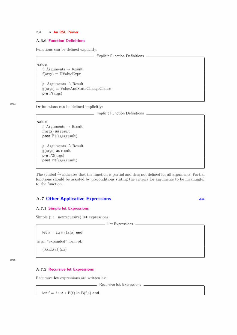
204 A An RSL Primer
A.6.6 Function Definitions
Functions can be defined explicitly:
Explicit Function Definitions
valuef: Arguments → Resultf(args) ≡ DValueExpr
g: Arguments∼→ Result
g(args) ≡ ValueAndStateChangeClausepre P(args)
s963Or functions can be defined implicitly:
Implicit Function Definitions
valuef: Arguments → Resultf(args) as resultpost P1(args,result)
g: Arguments∼→ Result
g(args) as resultpre P2(args)post P3(args,result)
The symbol∼→ indicates that the function is partial and thus not defined for all arguments. Partial
functions should be assisted by preconditions stating the criteria for arguments to be meaningfulto the function.
A.7 Other Applicative Expressions s964
A.7.1 Simple let Expressions
Simple (i.e., nonrecursive) let expressions:
Let Expressions
let a = Ed in Eb(a) end
is an “expanded” form of:
(λa.Eb(a))(Ed)
s965
A.7.2 Recursive let Expressions
Recursive let expressions are written as:
Recursive let Expressions
let f = λa:A • E(f) in B(f,a) end

A.7 Other Applicative Expressions 205
is “the same” as:
let f = YF in B(f,a) end
where:
F ≡ λg•λa•(E(g)) and YF = F(YF)
s966
A.7.3 Predicative let Expressions
Predicative let expressions:
Predicative let Expressions
let a:A • P(a) in B(a) end
express the selection of a value a of type A which satisfies a predicate P(a) for evaluation in thebody B(a).
s967
A.7.4 Pattern and “Wild Card” let Expressions
Patterns and wild cards can be used:
Patterns
let a ∪ s = set in ... endlet a, ∪ s = set in ... end
let (a,b,...,c) = cart in ... endlet (a, ,...,c) = cart in ... end
let 〈a〉ℓ = list in ... endlet 〈a, ,b〉ℓ = list in ... end
let [ a 7→b ] ∪ m = map in ... endlet [ a 7→b, ] ∪ m = map in ... end
s968
A.7.5 Conditionals
Various kinds of conditional expressions are offered by RSL:
Conditionals
if b expr then c expr else a exprend
if b expr then c expr end ≡ /∗ same as: ∗/if b expr then c expr else skip end
if b expr 1 then c expr 1

206 A An RSL Primer
elsif b expr 2 then c expr 2elsif b expr 3 then c expr 3...elsif b expr n then c expr n end
case expr ofchoice pattern 1 → expr 1,choice pattern 2 → expr 2,...choice pattern n or wild card → expr n
end
s969
A.7.6 Operator/Operand Expressions
Operator/Operand Expressions
〈Expr〉 ::=〈Prefix Op〉 〈Expr〉| 〈Expr〉 〈Infix Op〉 〈Expr〉| 〈Expr〉 〈Suffix Op〉| ...
〈Prefix Op〉 ::=− | ∼ | ∪ | ∩ | card | len | inds | elems | hd | tl | dom | rng
〈Infix Op〉 ::== | 6= | ≡ | + | − | ∗ | ↑ | / | < | ≤ | ≥ | > | ∧ | ∨ | ⇒| ∈ | 6∈ | ∪ | ∩ | \ | ⊂ | ⊆ | ⊇ | ⊃ | | † |
〈Suffix Op〉 ::= !
A.8 Imperative Constructs s970
A.8.1 Statements and State Changes
Often, following the RAISE method, software development starts with highly abstract-applicativeconstructs which, through stages of refinements, are turned into concrete and imperative con-structs. Imperative constructs are thus inevitable in RSL.
Statements and State Change
Unitvalue
stmt: Unit → Unitstmt()
• Statements accept no arguments.• Statement execution changes the state (of declared variables).• Unit → Unit designates a function from states to states.• Statements, stmt, denote state-to-state changing functions.• Writing () as “only” arguments to a function “means” that () is an argument of type Unit.
s971

A.8 Imperative Constructs 207
A.8.2 Variables and Assignment
Variables and Assignment
0. variable v:Type := expression1. v := expr
A.8.3 Statement Sequences and skip
Sequencing is expressed using the ‘;’ operator. skip is the empty statement having no value orside-effect.
Statement Sequences and skip
2. skip3. stm 1;stm 2;...;stm n
A.8.4 Imperative Conditionals
Imperative Conditionals
4. if expr then stm c else stm a end5. case e of: p 1→S 1(p 1),...,p n→S n(p n) end
s972
A.8.5 Iterative Conditionals
Iterative Conditionals
6. while expr do stm end7. do stmt until expr end
A.8.6 Iterative Sequencing
Iterative Sequencing
8. for e in list expr • P(b) do S(b) end

208 A An RSL Primer
A.9 Process Constructs s973
A.9.1 Process Channels
Let A and B stand for two types of (channel) messages and i:KIdx for channel array indexes, then:
Process Channels
channel c:Achannel k[ i ]:B • i:KIdx
declare a channel, c, and a set (an array) of channels, k[i], capable of communicating values of thedesignated types (A and B).s974
A.9.2 Process Composition
Let P and Q stand for names of process functions, i.e., of functions which express willingness toengage in input and/or output events, thereby communicating over declared channels. Let P() andQ stand for process expressions, then:
Process Composition
P ‖ Q Parallel compositionP ⌈⌉⌊⌋ Q Nondeterministic external choice (either/or)P ⌈⌉ Q Nondeterministic internal choice (either/or)P –‖ Q Interlock parallel composition
express the parallel (‖) of two processes, or the nondeterministic choice between two processes:either external (⌈⌉⌊⌋) or internal (⌈⌉). The interlock (–‖) composition expresses that the two processesare forced to communicate only with one another, until one of them terminates.s975
A.9.3 Input/Output Events
Let c, k[i] and e designate channels of type A and B, then:
Input/Output Events
c ?, k[ i ] ? Inputc ! e, k[ i ] ! e Output
expresses the willingness of a process to engage in an event that “reads” an input, respectively“writes” an output.s976
A.9.4 Process Definitions
The below signatures are just examples. They emphasise that process functions must somehowexpress, in their signature, via which channels they wish to engage in input and output events.
Process Definitions
valueP: Unit → in c out k[ i ]UnitQ: i:KIdx → out c in k[ i ] Unit

A.10 Simple RSL Specifications 209
P() ≡ ... c ? ... k[ i ] ! e ...Q(i) ≡ ... k[ i ] ? ... c ! e ...
The process function definitions (i.e., their bodies) express possible events.
A.10 Simple RSL Specifications s977
Often, we do not want to encapsulate small specifications in schemes, classes, and objects, as isoften done in RSL. An RSL specification is simply a sequence of one or more types, values (includingfunctions), variables, channels and axioms:
Simple RSL Specifications
type...
variable...
channel...
value...
axiom...
s978


B
Indexes
B.1 Concept Index
abstractsyntax
analytic, 44synthetic, 44
typesyntax, 38, 44
abstraction, 23model-oriented, 38property-oriented, 38
accessibility, 168Ada, 3adaptive maintenance, 170, 171algebra, fn 3, 6alphabet, 39analogic model, 32analytic
model, 32, 33analytic abstract syntax, 44ASM, 181atomic
simple entity, 58, 59attribute, 7
of entity, 7simple entity
atomic, 58composite, 58continuous, 58
attribute, 58authorised user, 170auxiliary
function, 28, 29availability, 168, 169axiomatic
semantics, 51–52
B, 3, 31
behaviour, 56, 63, 167communicating, 63concurrent, 63human, 136
domain facet, 123–128parallel, 63sequential, 63
behaviouralsemantics, 49–50
black (opaque) box, 34black box, 34BNF, 39
grammar, 38, 39rule, 39
boxblack/opaque, 34glass/white/transparent, 34
BPI (business process improvement), 79business
process, 77engineering, 80improvement (BPI), 79re-engineering, 134
processes, 77–84
CafeOBJ, 181change management, 134channel, 63
CSP, 63character, 39code, 173composite
simple entity, 58, 59computer
science, 7computing

212 B Indexes
science, 7concept, 5concrete
typesyntax, 38, 41
connotation, 34continuous
simple entity, 58contract
domain facet, 98–123corrective maintenance, 170, 171CSP, 3
DCduration calculus, 4, 93, 181, 228
definitionof function, 66
demonstration platformrequirements, 172
demonstration platform requirements, 172denotation, 34denotational
semantics, 47–49dependability, 167
attribute, 168tree, 168
descriptioninformal, 27ontology, 56
descriptivemodel, 32, 33
determinationof domain, 145
developmentdocument, 173logbook, 173platform requirements, 172
discretesimple entity, 59
documentdescription, informal, 27informative
synopsis, 27documentation
requirements, 173domain
action, 63contract
facet, 98–123description, 173
non-normative, 17determination, 145engineering, 20extension, 149
facet, 77human behaviour, 77, 123–128intrinsics, 77, 78management and organisation, 77, 93–
96rules and regulations, 77, 96–98scripts, 77support technologies, 77support technology, 88–93
fitting, 150instantiation, 144intrinsics, 78, 84–88, 136license
facet, 98–123management and organisation
facet, 93–96ontology, 56projection, 142rules and regulations
facet, 96–98science
versus physics, 6–7script
facet, 98–123state, 63support technology
facet, 88–93domain
description, 5science, 5, 7what is a, 5–18
engineeringbusiness process, 80rules and regulations, 138
entity, 56entity
behaviour, 56event, 56function, 56simple, 56
error, 167event, 56, 68–69execution platform requirements, 172extension
of domain, 149extensional
maintenance, 170, 171model, 32, 34
facetcontract, 98–123domain
human behaviour, 123–128

CONCEPT INDEX 213
intrinsics, 77, 78management and organisation, 77rules and regulations, 77scripts, 77support technologies, 77
domain, human behaviour, 77intrinsics, 84–88license, 98–123management and organisation, 93–96rules and regulations, 96–98script, 98–123support technology, 88–93
failure, 167fault, 167, 168
forecasting, 168prevention, 168removal, 168tolerance, 168
fittingof domain requirements, 150
function, 66–67auxiliary, 28, 29definition, 66invocation, 66signature, 66
glass (transparent) box, 34glass box, 34golden rule of requirements, 133grammar
BNF, 38, 39
human behaviour, 136domain facet, 77, 123–128re-engineering, 139
iconic model, 32, 33ideal rule of requirements, 133indicative, 33individual
= entity, 56informal description, 27informative document
synopsis, 27infrastructure, 19input
CSP, ch ?, 63installation
manual, 173instantiation
of domain, 144integrity, 168, 169intensional model, 32, 34intrinsics
domain, 78, 136domain facet, 77, 84–88requirements, 136review and replacement, 137
invocationof function, 66
knowledgeengineering, 7
licensedomain facet, 98–123
locationspatial attribute, 7
logical atomismRussell, 56
LSClive sequence charts, 80, 93, 181
machinerequirements, 165
maintenanceadaptive, 170, 171corrective, 170, 171extensional, 170, 171logbook, 173manual, 173perfective, 170, 171preventive, 170, 171requirements, 170
maintenance platformrequirements, 172
managementand organisation, 136
re-engineering, 138of change, 134
management and organisationdomain facet, 77, 93–96
manualinstallation, 173maintenance, 173training, 173user, 173
mereology, 59semantic, 64–66syntactic, 60–63
mereology, 60metaphysics
Russell, 55methodology
Russell, 55model, 31model-oriented abstraction, 38modelling, 31

214 B Indexes
MSCmessage sequence charts, 3, 63, 80, 93,
181, 228
non-terminal, 39noumenon, fn. 1, 5
ontologydescription, 56domain, 56
ontology, 56opaque (black) box, 34operation, 56organisation
and management, 136re-engineering, 138
outputCSP, ch
e, 63
particular= entity, 56
perfective maintenance, 170, 171performance requirements, 165Petri net, 3, 63, 80, 93, 181, 228phenomenon, 5platform requirements, 172
demonstration, 172development, 172execution, 172maintenance, 172
pragmatics, 52–53prescriptive model, 32, 33preventive maintenance, 170, 171process
CSP, 63business, 77channel, 63engineering, 80invocation, 63re-engineering, 134state, 63
projectionof domain, 142
property-oriented abstraction, 38putative, 33
RAISE, 3, 18, 31, 55, 181re-engineering
business process, 134human behaviour, 139management and organisation, 138rules and regulations, 139script, 139
regulationsand rules, 136
re-engineering, 138, 139reliability, 168, 169requirements, 133
demonstration platform, 172determination, of domain, 145development
platform, 172documentation, 173engineering, 20execution platform, 172extension, of domain, 149fitting, of domain, 150golden rule, 133ideal rule, 133instantiation, of domain, 144intrinsics, 136machine, 165maintenance, 170
platform, 172performance, 165platform, 172prescription, 173projection, of domain, 142
review and replacementintrinsics, 137support technology, 137
robustness, 168, 170rough sketch
a preparatory document, 78rough sketching, 77–78RSL, 3, 18, 31, 55, 181rule
BNF, 39rules
and regulations, 136re-engineering, 138, 139
rules and regulationsdomain facet, 77, 96–98
RussellLogical Atomism, 55–56logical atomism, 56metaphysics, 55methodology, 55
safety, 168, 169script
domain facet, 98–123re-engineering, 139
scripting, 136scripts
domain facet, 77security, 168, 170

DEFINITION INDEX 215
semantic type, 45semantics, 46–52
axiomatic, 51–52behavioural, 49–50denotational, 47–49of programming languages, 3
semiotics, 37–53signature
of function, 66simple entity, 7, 56, 57
atomic, 58, 59composite, 58, 59continuous, 58discrete, 59
simple use ofCSP, 4abstract types, 3concrete types, 3discrete mathematics, 3mathematical logic, 3model-oriented abstractions, 3pragmatics, 3property-oriented abstractions, 3semantics, 3semiotics, 3syntax, 3
sketch, rough, 78software
design, 173engineering
education, proper, 3practice of, 3
spatial attribute, 7state
of a system, 27of domain, 63
Statechart, 3, 63, 80, 93, 181, 228sub-entity, 59support
document, 173technology, 136
support technologiesdomain facet, 77
support technologydomain facet, 88–93review and replacement, 137
synopsis, 27
syntactic type, 45syntax, 38–46
abstracttype, 38, 44
concretetype, 38, 41
synthetic abstract syntax, 44system
state, 27
technologysupport, 136
terminal, 39test
document, 173TLA+, temporal logic of actions, 4, 93, 181,
228tool
of domain science and engineering, 6training manual, 173transparent (glass) box, 34transparent (white) box, 34type
abstractsyntax, 38, 44
concretesyntax, 38, 41
semantic, 45syntactic, 45
un-authorised user, 170universe of discourse, 31user
authorised, 170manual, 173un-authorised, 170
validationdocument, 173
VDM, 3VDM, 3, 31, 181verification
document, 173of programs, 3
white box, 34
Z, 3, 31, 181
B.2 Definition Index
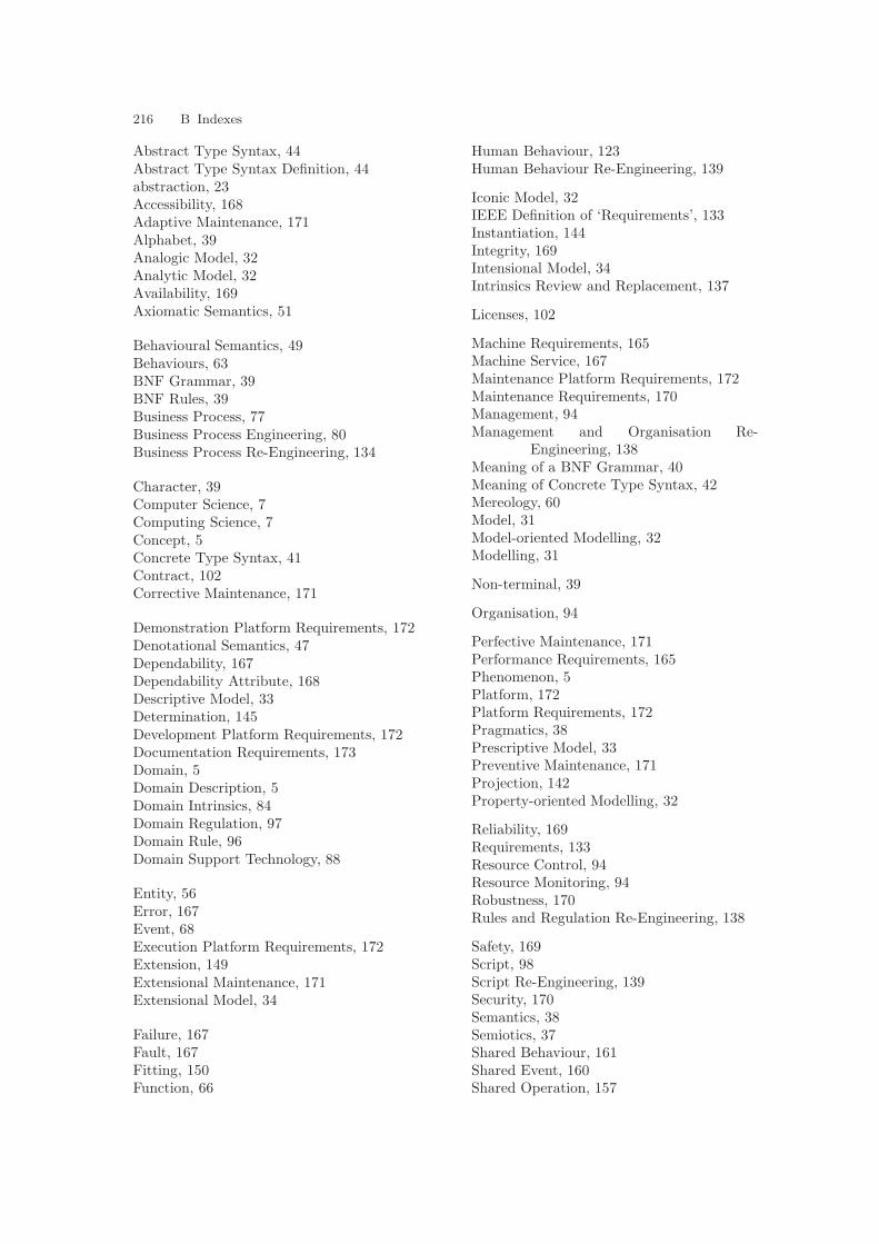
216 B Indexes
Abstract Type Syntax, 44Abstract Type Syntax Definition, 44abstraction, 23Accessibility, 168Adaptive Maintenance, 171Alphabet, 39Analogic Model, 32Analytic Model, 32Availability, 169Axiomatic Semantics, 51
Behavioural Semantics, 49Behaviours, 63BNF Grammar, 39BNF Rules, 39Business Process, 77Business Process Engineering, 80Business Process Re-Engineering, 134
Character, 39Computer Science, 7Computing Science, 7Concept, 5Concrete Type Syntax, 41Contract, 102Corrective Maintenance, 171
Demonstration Platform Requirements, 172Denotational Semantics, 47Dependability, 167Dependability Attribute, 168Descriptive Model, 33Determination, 145Development Platform Requirements, 172Documentation Requirements, 173Domain, 5Domain Description, 5Domain Intrinsics, 84Domain Regulation, 97Domain Rule, 96Domain Support Technology, 88
Entity, 56Error, 167Event, 68Execution Platform Requirements, 172Extension, 149Extensional Maintenance, 171Extensional Model, 34
Failure, 167Fault, 167Fitting, 150Function, 66
Human Behaviour, 123Human Behaviour Re-Engineering, 139
Iconic Model, 32IEEE Definition of ‘Requirements’, 133Instantiation, 144Integrity, 169Intensional Model, 34Intrinsics Review and Replacement, 137
Licenses, 102
Machine Requirements, 165Machine Service, 167Maintenance Platform Requirements, 172Maintenance Requirements, 170Management, 94Management and Organisation Re-
Engineering, 138Meaning of a BNF Grammar, 40Meaning of Concrete Type Syntax, 42Mereology, 60Model, 31Model-oriented Modelling, 32Modelling, 31
Non-terminal, 39
Organisation, 94
Perfective Maintenance, 171Performance Requirements, 165Phenomenon, 5Platform, 172Platform Requirements, 172Pragmatics, 38Prescriptive Model, 33Preventive Maintenance, 171Projection, 142Property-oriented Modelling, 32
Reliability, 169Requirements, 133Resource Control, 94Resource Monitoring, 94Robustness, 170Rules and Regulation Re-Engineering, 138
Safety, 169Script, 98Script Re-Engineering, 139Security, 170Semantics, 38Semiotics, 37Shared Behaviour, 161Shared Event, 160Shared Operation, 157

B.3 Example Index 217
Shared Simple Entity, 153Simple Entity, 57Strategy, 93Support Technology Review and Replace-
ment, 137
Syntax, 37
Tactics, 93
Terminal, 39
B.3 Example Index
“The Market”, 8
A Behavioural Semantics, 50A Bus Services Contract Language, 108A Business Plan Business Process, 78A Casually Described Bank Script, 123A Comprehensive Set of Administrative
Business Processes, 79A Concrete Type Syntax: Banks, 41A Denotational Language Semantics: Banks,
47A Domain Example: an ‘Airline Timetable
System’, 141A Formally Described Bank Script, 124A Health Care License Language, 103A Human Behaviour Mortgage Calculation,
125A Public Administration License Language,
105A Purchase Regulation Business Process, 79A Telephone Exchange, 27A Toll-road System (I), 139Air Traffic (I), 8Air Traffic (II), 89Air Traffic Business Processes, 81Alphabet, 39An Abstract Type Syntax: Arithmetic Ex-
pressions, 44An Abstract Type Syntax: Banks, 45An Axiomatic Semantics: Banks, 51An Oil Pipeline System, 84Analogic, Analytic and Iconic Models, 32Atomic Entities, 59Attributes, 58
Bank Staff or Programmer Behaviour, 125Banking, 8BNF Grammar: Banks, 40BNF Rules, 39
Characters, 39Comparison: Abstract and Concrete Banks,
46Composite Entities (1), 59
Composite Entities (2), 59Container Line Industry, 8Continuous Entities, 58
Descriptive and Prescriptive Models, 33Determination: A Road Maintenance Sys-
tem, 148Determination: A Toll-road System, 148Discrete Entities, 59Domain Types and Observer Functions, 152
Entities and Behaviours, 63Extension: A Toll-road System, 150Extensional Model Presentations, 34External Events, 68
Financial Service Industry Business Pro-cesses, 82
Fitting: Road Maintenance and Toll-roadSystems, 151
Freight Logistics Business Processes, 82
Harbour Business Processes, 82Health Care, 8Health-care Script Re-Engineering, 139Hospital Information System Security, 170Human Behaviour Re-Engineering, 139
Instantiation: A Road Maintenance System,144
Instantiation: A Toll-road System, 144Intensional Model Presentations, 34Interesting Internal Events, 68Intrinsics Replacement, 137
Management and Organisation, 94Management and Organisation Re-
Engineering, 138Meaning of a BNF Grammar, 41Mereology: Parts and Wholes (1), 60Mereology: Parts and Wholes (2), 64Model-oriented Directory, 24
Networked Social Structures, 24Non-terminals, 39
Oil Industry, 8

218 B Indexes
Pragmatics: Banks, 52Projection: A Road Maintenance System, 142Projection: A Toll-road System, 143Public Government, 8
Rail Track Train Blocking, 97Railway and Train Business Processes, 83Railway Nets, 24Railway Switch Support Technology, 88Railways, 9Representation of Transport Net Hubs, 154Requirements Types and Decompositions,
152Road System, 9Rules and Regulations Re-Engineering, 138
Shared Behaviours: Personal FinancialTransactions, 161
Shared Operations: Personal FinancialTransactions, 157
Shared Simple Entities: Railway Units, 153Shared Simple Entities: Toll-road Units, 153Shared Simple Entities: Transport Net Data
Initialisation, 155Shared Simple Entities: Transport Net Data
Representation, 153Simple Entities, 57
Space Satellite Software Platforms, 172Storage and Speed for n-Transfer Travel In-
quiries, 167Street Intersection Signalling, 89Support Technology Review and Replace-
ment, 137
Terminals, 39Timetable Accessibility, 169Timetable Availability, 169Timetable Reliability, 169Timetable Safety, 169Timetable Security, 170Timetable System Adaptability, 171Timetable System Correct-ability, 171Timetable System Determination, 146Timetable System Extendability, 171Timetable System Extension, 149Timetable System Perfectability, 171Timetable System Performance, 165Timetable System Users and Staff, 166Timetables, 98Trains Entering and/or Leaving Stations, 97Transport Net (I), 9Transport Net (II), 55Transport Net Building, 126
B.4 Symbol Index
Literals, 199–208Unit, 208chaos, 199, 200false, 192, 194true, 192, 194
Arithmetic Constructs, 195ai*aj, 195ai+aj, 195ai/aj, 195ai=aj, 195ai≥aj, 195ai>aj, 195ai≤aj, 195ai<aj, 195ai 6=aj, 195ai−aj, 195
Cartesian Constructs, 196, 199(e1,e2,...,en), 196
Combinators, 204–207
... elsif ..., 206do stmt until be end, 207for e in listexpr • P(b) do stm(e) end, 207if be then cc else ca end , 205–206let a:A • P(a) in c end, 205let pa = e in c end, 205variable v:Type := expression, 207while be do stm end, 207v := expression, 207
Function Constructs, 190post P(args,result), 190pre P(args), 190f(args) as result, 190f(a), 188f(args) ≡ expr, 190f(), 192
List Constructs, 196, 199–201<Q(l(i))|i in<1..lenl> •P(a)> , 196e1 <e2,e2,...,en > ,196<> , 196–201
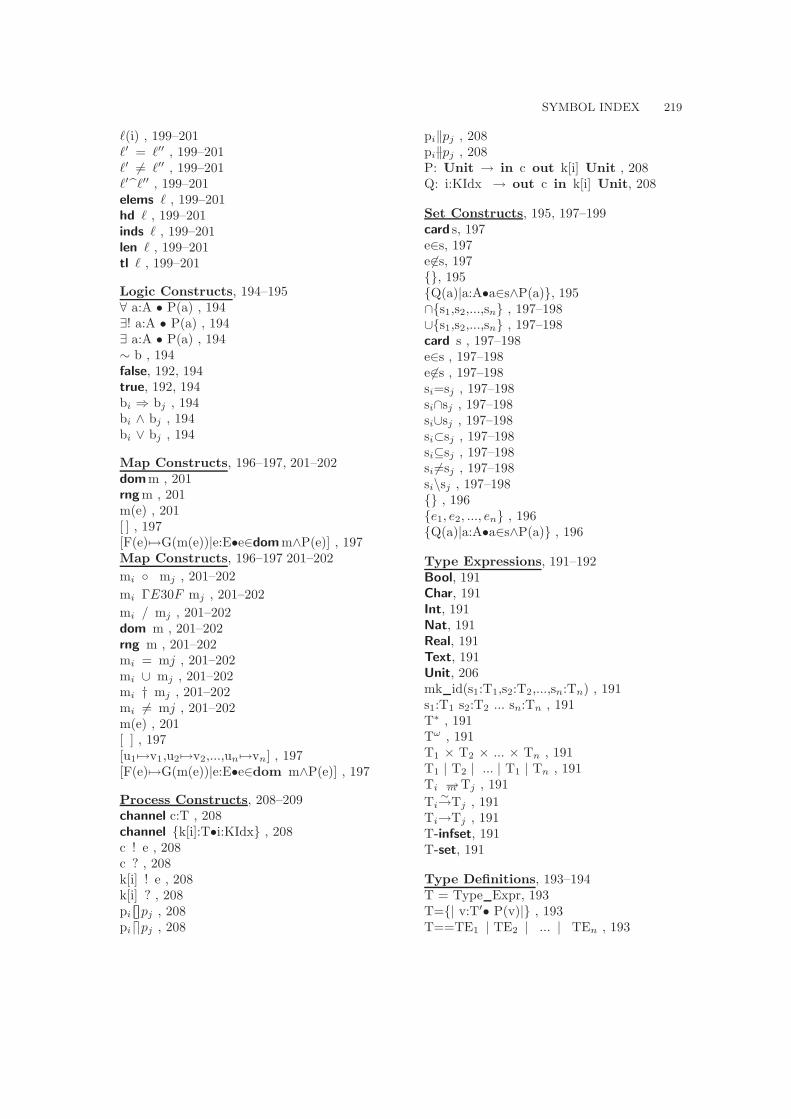
SYMBOL INDEX 219
ℓ(i) , 199–201ℓ′ = ℓ′′ , 199–201ℓ′ 6= ℓ′′ , 199–201ℓ′ℓ′′ , 199–201elems ℓ , 199–201hd ℓ , 199–201inds ℓ , 199–201len ℓ , 199–201tl ℓ , 199–201
Logic Constructs, 194–195∀ a:A • P(a) , 194∃! a:A • P(a) , 194∃ a:A • P(a) , 194∼ b , 194false, 192, 194true, 192, 194bi ⇒ bj , 194bi ∧ bj , 194bi ∨ bj , 194
Map Constructs, 196–197, 201–202domm , 201rngm , 201m(e) , 201[ ] , 197[F(e)7→G(m(e))|e:E•e∈domm∧P(e)] , 197Map Constructs, 196–197 201–202
mi mj , 201–202
mi ΓE30F mj , 201–202
mi / mj , 201–202dom m , 201–202rng m , 201–202mi = mj , 201–202mi ∪ mj , 201–202mi † mj , 201–202mi 6= mj , 201–202m(e) , 201[ ] , 197[u1 7→v1,u2 7→v2,...,un 7→vn] , 197[F(e)7→G(m(e))|e:E•e∈dom m∧P(e)] , 197
Process Constructs, 208–209channel c:T , 208channel k[i]:T•i:KIdx , 208c ! e , 208c ? , 208k[i] ! e , 208k[i] ? , 208pi⌈⌉⌊⌋pj , 208pi⌈⌉pj , 208
pi‖pj , 208pi–‖pj , 208P: Unit → in c out k[i] Unit , 208Q: i:KIdx → out c in k[i] Unit, 208
Set Constructs, 195, 197–199card s, 197e∈s, 197e 6∈s, 197, 195Q(a)|a:A•a∈s∧P(a), 195∩s1,s2,...,sn , 197–198∪s1,s2,...,sn , 197–198card s , 197–198e∈s , 197–198e 6∈s , 197–198si=sj , 197–198si∩sj , 197–198si∪sj , 197–198si⊂sj , 197–198si⊆sj , 197–198si 6=sj , 197–198si\sj , 197–198 , 196e1, e2, ..., en , 196Q(a)|a:A•a∈s∧P(a) , 196
Type Expressions, 191–192Bool, 191Char, 191Int, 191Nat, 191Real, 191Text, 191Unit, 206mk id(s1:T1,s2:T2,...,sn:Tn) , 191s1:T1 s2:T2 ... sn:Tn , 191T∗ , 191Tω , 191T1 × T2 × ... × Tn , 191T1 | T2 | ... | T1 | Tn , 191Ti →m Tj , 191
Ti∼→Tj , 191
Ti→Tj , 191T-infset, 191T-set, 191
Type Definitions, 193–194T = Type Expr, 193T=| v:T′• P(v)| , 193T==TE1 | TE2 | ... | TEn , 193


Part VIII
Lecturers Material
The next two appendices are not part of the book as published, but is provided, in principle, onlyto lecturers.


C
Lecturers’ Guide to Using This Book
Pages XIII–XIV suggests a 14-18 lectures schedule. Slight variants of this schedule has been lec-tured over at
• National University of Singapore (NUS), in the spring of 2005 (RSL),• Japan Advanced Institute of Science and Technology (JAIST), in the fall of 2006 (CafeOBJ),• University of Henri Poincare/INRIA at Nancy, France, in the fall of 2007 (Event B),• Technical University of Graz, Austria, in the fall of 2008 (Alloy),• University of Saarland, Saarbrucken, Germany, March 2009 (Discrete Mathematics),• University of Edingburgh, Scotland, September–October 2009 (Discrete Mathematics), and• Tokyo University, Japan, Nov.–December 2009 (Alloy).
C.1 Narratives and Formalisations
• It is a major characteristic of this textbook and the approach to software engineering that itadvocates that descriptions (of domains), prescriptions (of requirements) and specifications ofsoftware — although we do not cover software design — is expressed both informally, throughcarefully crafted narratives, and formally, in this textbook through the use of the RAISE formalspecification language RSL.
• But it is also a — perhaps strange — characteristic of this textbook that we do not “teach”RSL.⋆ That is: we do not introduce RSL from “first principles” !⋆ Instead we just present the formal parts of most examples in the RSL notation.⋆ To alleviate “the chock” that such formulas as RSL enables us to write, we annotate, that
is, carefully explain these formalisations, line-by-line, RSL-construct-by-RSL-construct.⋆ This is done in Example 10 (starting Page 9).⋆ These annotations are there related to the places in the RSL Primer of Appendix A.
• In the courses given around the world in the last five years, and listed above, the studentprojects have used various formal notations. These are listed in parentheses above.
• This leaves either a burden on the lecturer or it does not leave such a burden:⋆ Either the lecturer, with the students, must decide on a formal specification language —
for the case that no such is taught at the lecturer’s institution;⋆ or the lecturer — for the case that at least one formal notation has been introduced to
students in some earlier courses — chooses such a notation.• In any case: the students, at the end of a course, based on the present textbook, should have
reasonably strong motivations for and skills in using formal notations.• These are potentially good such systems of notations:

224 C Lecturers’ Guide to Using This Book
⋆ Alloy [90]⋆ Event B [2]⋆ RSL [17]
⋆ Spec# [10]⋆ VDM [57]⋆ Z [145]
C.2 Use of Textbook
• Since the lecture slides, see next section, Sect. C.3, only present very essentials of the textlecturers must study the textbook carefully and students should regularly consult the textbook:the latter by (students) attempting to more-or-less cursorily read the relevant text before thelecture and by re-reading it after the lecture.
• The textbook provides more than 80 pages of examples scattered all over the text. An ‘ExamplesIndex’, Sect. B.3 (Pages 217–218), lists all examples by ‘Example Name’. The lecturer neednot cover all these examples.
• Lecturers’ version of the textbook1 provides display line and margin references to the approx-s#i
imately 900 ‘Lecture Slides’: s#i is placed at book text (some of) which also appears on slide#i.
• Lectures based on — and studies of — the textbook rely on the students and readers alsopursuing one of the projects listed in Sect. D.2. To that end each chapter of the textbookrefers to project exercise items listed in Sect. D.1. There is at least one project exercise itemper lecture. In other words: the lecturer is well advised in making sure to emphasise themethodology underlying solutions to these project exercise items.
C.3 Use of Lecture Slides
• Textbook Pages XIII–XIV provide a proposal for composing a course of the textbook in theform of between 14 and 18 lectures.
• Lecturers can obtain, from the publisher, access to “pre-packaged” sets of lecture slides, ineither postscript or pdf form.
• For reasons of copyright it is not possible to provide students with access to electronic versionsof these slides.2
• Some of the proposed lectures may seem a bit long for a session of two 45–50 minute lectures.The lecturer must decide on this length and may therefore be forced to carefully decide whetherto skip some examples (which is advised) or to skip some methodology text (which may bepossible). In such a case it may be possible for the lecturer to prepare a lecture (.ps or .pdf)file with just a subset of the pages of the “pre-packaged” lecture files.
• All examples contain both itemized or enumerated narrative, English text and, on subsequentslides, oftentimes enumerated formulas. In early lectures it is advised to first “read” the nar-rative texts, then show (or “read)) the formulas. In later lectures the lecturer can skip thenarrative texts and “narrate” the formulas (as if they were their narrative counterparts). Thusbasically half the examples slides can be omitted in most lectures.
• The point to be made here, by the lecturer — since it is being made by the book (and itsauthor) — is that (even model-oriented) formal specifications can be “naturally” read, thatis, as if they were narratives. (But formalisations can never replace the narratives: the lattermust be expressed in such a way as to provide for easy understanding (i.e., reading) by allstake-holders.
1This ‘Lecturers Version’ is available, electronically, upon request, from the publisher.2The author will try persuade the publisher to allow publisher-registered lecturers to give their students
read-access to lecturers’ slides during the lecturing and pre-exam period.

C.5 Lecture-by-Lecture Guide 225
C.4 A Single or A Two Semester Course
This textbook can be used for
• either a single semester course covering all lectures• or for two single semester courses
⋆ Basic Concepts and Domain Engineering, Lectures 1-11,⋆ Requirements Engineering, Lectures 12-18.
• In the latter version the ‘requirements engineering lectures’ can be combined with a course insome specific problem frame such as outlined in Appendix Sect. D.2.2:
⋆ Reactive Systems⋆ Workpiece Systems
⋆ Transformation Systems⋆ Information Systems
or other.
C.5 Lecture-by-Lecture Guide
Each lectures consists of two sessions, A and B. Each should present a well-formed set of a fewtopics.
C.5.1 Lecture 1
This lecture is partly for the coverage of the below-listed front- and main-matter pages of thetextbook, partly for the familiarisation of course lecturer and course students, including detailsabout the course project and formation of course project groups.
A: Opening XII–XIII
Comment, lightly, on the 15–18 lectures ahead.
B: Background 3–4
Spend time on informally discussing with students about the formation of project groups.
C.5.2 Lecture 2
C: What are Domains ? 5–18
D: Motivation for Domain Engineering 19–20
C.5.3 Lecture 3: Abstraction & Modelling (I)
Chapter 4: Lectures 3[A–B] is covered by initial parts of Sect. 4.1.
A: Abstraction 23–24
Cover the definition of abstraction, top of Page 23. Emphasise “omission of details” and “focus onwhat is important”.
Discuss the ideas of phenomena and concepts. Discuss the duality of narratives versus formal-isations.
Go carefully through the narratives and explaining the RSL notation of the formalisation ofExamples 11–12.

226 C Lecturers’ Guide to Using This Book
B: Abstraction 24–27
Go carefully through the narrative and explain the RSL notation of the formalisation of Example 13.Close by reminding the student of Example 10. Ask them to study the similarity of Example 10and Example 13.
C.5.4 Lecture 4 Abstraction & Modelling (II)
Chapter 4. Lecture 4[A] is covered by remaining parts of Sect. 4.1. Lecture 4[B] covers Sect. 4.2.
A: Abstraction27–31
B: Modelling31–35
C.5.5 Lecture 5: Semiotics
Chapter 5: Lecture 5[A] is covered by Sects. 5.1–5.2. Lecture 5[B] is covered by Sects. 5.3–5.5.
A: Syntax37–46
B: Semantics and Pragmatics46–53
C.5.6 Lecture 6: A Specification Ontology – I
Chapter 6: Lecture 6[A] is covered by Sects. 6.1–6.3.1, and Lecture 6[B] is covered by Sect. 6.3.2.
A:55–63
B:63–66
C.5.7 Lecture 7: A Specification Ontology – II
Chapter 6: Lectures
A:66–69
B:69–73
C.5.8 Lecture 8: Domain Engineering – I
Chapter 7: Lectures
A: Opening Stages77–84
B: Intrinsics84–88
C.5.9 Lecture 9: Domain Engineering – II
Chapter 7: Lectures
A: Supp.Techns.88–93
B: Mgt. & Org.93–96
C.5.10 Lecture 10: Domain Engineering – III
Chapter 7: Lectures

C.6 Commensurate Formalisations 227
A: Rules & Regs.96–98
B: Scripts98–123
C.5.11 Lecture 11: Domain Engineering – IV
Chapter 7: Lectures
A: Human Behaviour 123–128
B: Closing Stages 128–129
C.5.12 Lecture 12: Requirements Engineering – I
Chapter 8: Lectures
A: Opening Stages and Acquisition 133–134
B: Business Processes 134–141
C.5.13 Lecture 13: Requirements Engineering – II
Chapter 8: Lectures
A: Domain Requirements 141–145
B: Domain Requirements 145–153
C.5.14 Lecture 14: Requirements Engineering – III
Chapter 8: Lectures
A: Interface Requirements 153–156
B: Interface Requirements 157–164
C.5.15 Lecture 15: Requirements Engineering – IV
Chapter 8: Lectures A-B-C
A: Machine Requirements 165–173
B: Closing Stages 173–174
A: Closing 177–177
C.6 Commensurate Formalisations
• Natural language narratives have the strength to describe (and prescribe) all that need be sospecified.⋆ But natural language narratives are apt to be ambiguous,⋆ that is, not sufficently precise, and do not allow formal proofs of properties.
• Formal specification languages, on the other hand, are not capable of formalising, at least notelegantly, all that can be narrated.⋆ Therefore we augment formal specifications given in one, say the “major” notation,⋆ with formalisations given in other notations.

228 C Lecturers’ Guide to Using This Book
⋆ Some examples of such other formalisations are:· Duration Calculus [148,149] (suitable for the formalisation of real-time [safety critical]
properties),· Petri Nets [91, 115,123–125] (suitable for the formalisation of concurrent properties),· Message Sequence Charts (MSC) [86–88] (suitable for the formalisation of concurrent
properties),· Statecharts [71–74,76] (suitable for the formalisation of concurrent properties), and· TLA+ [96, 97, 105, 106] (suitable for the formalisation of real-time [safety critical] prop-
erties).• Oftentimes lecturers are specialists in one or another of these notations.• The projects (listed in Appendix Sect. D.2) usually require the full spectrum of one of the
specification languages mentioned at the end of Sect. C.1 as well as one or more of the above-listed notations (which include some very appealing diagrammatic notational systems).

D
Lecturers’ Guide to Projects
This book contains only one exercise. Normally exercises are listed at the end of each chapter.Instead we shall use this appendix to outline a number of project topics and how the reader(including course students) might tackle one of these projects.
The purpose of a student project is for student groups to document the degree to which they,as a group, have understood the lectures cum this textbook.
The form of a student project is a report. That report is to be like the proper development ofa domain description and the proper development of a requirements prescription: Narrative andformalisation. The formalisation is in some “more-or-less” formal notation chosen by the full setof course project students.
It may come as a surprise to you: the lecturer and/or the students, namely that we do notmandate the use of the RAISE specification language RSL. As also mentioned in the textbook: thereare other formal specification languages — and there is always plain old good mathematics !
Which formal specification language do I advocate ?Well these are potentially good such systems of notations:
• Alloy [90]• Event B [2]• RSL [17]
• Spec # [10]• VDM [57]• Z [145]
D.1 Project Assignments: Textbook Topic-by-Topic
This section, although part of lecturers material not (usually) contained in students’ material, isaddressed – as if – directly at project students.
There are two ways in which a project makes sense: either, for a self-study, by a motivatedreader, or, as a similarly indispensable part of a course.
The idea is, for students, to first choose one of the project or sub-project topics listed inSect. D.2 (take a brief, that is, hasty look at bold-faced terms of that list now); then, as lectures(and/or your reading of the textbook) progresses, from section-to-section, that is from methodologytopic-to-topic, you, the student, try apply the method covered by these sections to the chosenproject. This means that when you, the student, have studied the referenced sections itemizedbelow then you, the student, try your hand at the “exercises” written in slanted text next to thesection references:
1. Chapter 2, Sect. 2.2:
Formulate the essence of your chosen, i.e., the project domain.
Cf. Examples 1–9 (Pages 8–9).
2. Chapter 2, Sect. 2.3:

230 D Lecturers’ Guide to Projects
Enumerate informal, that is natural (i.e., national) language descriptions which everphenomena (entities, operations, events, behaviour) comes to your mind.
Try sort your enumerated list such that simplest facts are described first (needing no referenceto facts defined later), etc. — as in Example 10.
3. Chapter 4, Sect. 4.1.3 (Pages 23–31). Even though you may not yet be (fully) capable offormalising your chosen abstractions:
Identify two or three domain phenomena (or concepts) for each of which you thenconceive of a suitable abstraction and narrate and, however “feebly” formalise it.
Cf. the style of Examples 11–14 of Sect. 4.1.3, Pages 24–31).
4. Chapter 4, Sects. 4.2–4.3:
Discuss, for your chosen two or three examples, resulting from your solution to Item 3,the following attributes of your solutions:• model-orientedness versus property-orientedness1,• analogic, analytic and iconic,• descriptive (if a domain specification) and prescriptive (if a requirements specifica-
tion), and• extensional and intentional.
5. Chapter 5, Sect. 5.2:
Narrate and formalise concrete syntax(es) as well as abstract syntax(es) for at leastone syntactic type and at least one semantic type for chosen (however small) andrespective phenomena (or concepts) of your chosen domain.
That is, continue now towards further and further descriptions of your chosen domain.
6. Chapter 5, Sect. 5.3:
Narrate and formalise one denotational and one behavioural semantics for chosen (how-ever small) and respective phenomena (or concepts) of your chosen domain.
As for Item 5: continue now towards further and further descriptions of your chosen domain.
7. Chapter 6, Sect. 6.3.1:
Identify a small number of (hitherto not already identified) atomic and a small numberof composite simple entities and narrate and formalise these,
whileemphasising, in your narration, which are attributes, which are sub-entities and whichare mereologies of your described composite simple entities — as well as which are theattributes of atomic simple entities.
Make sure that your enumerated narrative statements “fit, hand-in-glove” with similarly enu-merated formulas.
8. Chapter 6, Sect. 6.4.1:
Identify a small number of (hitherto not already identified) domain operations, nar-rate and formalise these, both by explicit model-oriented definitions and by pre/postconditions.
Make sure that your enumerated narrative statements “fit, hand-in-glove” with similarly enu-merated formulas.
9. Chapter 6, Sect. 6.4.2:
Identify a small number of (hitherto not already identified) domain events.
Later, as part of your answer to Item 10, you shall then also formalise these events.
10. Chapter 6, Sect. 6.3.2:
Identify a small number of (hitherto not already identified) domain behaviours andnarrate and formalise these
1(that is, try have your solutions to Item 3 questions reflect a suitable combination of these and thefurther attributes as covered in Sect. 4.3)

D.1 Project Assignments: Textbook Topic-by-Topic 231
while including the formalisation of identifier domain events as identified in Item 9.
11. Chapter 7, Sect. 7.2:
Identify a small number of (hitherto not already identified) business processes andprovide rough sketch narratives.
12. Chapter 7, Sect. 7.3:
Identify a small number of (hitherto not already identified) domain intrinsic facets andnarrate and formalise these.
13. Chapter 7, Sect. 7.4:
Identify a small number of (hitherto not already identified) domain support technologyfacets and narrate and formalise these.
14. Chapter 7, Sect. 7.5:
Identify a small number of (hitherto not already identified) domain management andorganisation facets and narrate and formalise these.
15. Chapter 7, Sect. 7.6:
Identify a small number of (hitherto not already identified) domain rules and regula-tions facets and narrate and formalise these.
16. Chapter 7, Sect. 7.7:
Identify a small number of (hitherto not already identified) domain script (license orcontract) facets and narrate and formalise these.
17. Chapter 7, Sect. 7.8:
Identify a small number of (hitherto not already identified) human behaviour facetsand narrate and formalise these.
18. Chapter 7, Sects. 7.1–7.9:
Consolidate your narratives and formalisations of the answers to Items 11–17 into anice, clean, well-structured domain description.
It is OK to leave some operations, events and behaviours only “hinted at”, but the idea thata completion is straightforward should be convincing.
19. Chapter 8, Sect. 8.5:
Rough sketch (i.e., narrate) two reasonably distinct business process re-engineerings.
20. Chapter 8, Sect. 8.6:
Develop, based on the answer to Item 19, and in stages of development, a domainrequirements: projection, instantiation, determination, extension and fitting.
21. Chapter 8, Sect. 8.8:
Identify shared entities, operations, events and behaviours, and suggest, narrate andformalise
shared entity initialisation and refreshment requirements,shared operation requirements andshared event and behaviour requirements.
22. Chapter 8, Sects. 8.1–8.10:
Consolidate your narratives and formalisations of the answers to Items 19–21 into anice, clean, well-structured domain description.
It is OK to leave some operations, events and behaviours only “hinted at”, but the idea thata completion is straightforward should be convincing.
23. Page XI: The Triptych Phases:
Name the three phases of software engineering.
24. Chapter 7, Sect. 7.9: The Domain Engineering Stages:
Name 7–9 of the stages of domain engineering.Give a 1-3 line characterisation of 5–6 of the domain engineering stages.
25. Chapter 7, Sect. 7.1 (Sects. 7.2–7.8): The Main Facets of Domain Modelling:

232 D Lecturers’ Guide to Projects
Name 5–6 facets of domain modelling.Give a 1-3 line characterisation of the domain modelling facets.
26. Chapter 8, Sect. 8.10: The Requirements Engineering Stages:
Name 7–9 of the stages of requirements engineering.Give a 1-3 line characterisation of 5–6 of the requirements engineering stages.
27. Chapter 8, Sect. 8.2: The Core Stages of Requirements Modelling:
Name the core stages of requirements modelling.Give a 1-3 line characterisation of these stages of requirements modelling.
28. Chapter 8, Sect. 8.6: The Main Facets of Domain Requirements Modelling:
Name 4–5 facets of domain requirements modelling.Give a 1-3 line characterisation of each the these facets of domain requirements mod-elling.
29. Chapter 8, Sect. 8.8: The Three Facets of Interface Requirements Engineering:
Name the three facets of interface requirements modelling.Give a 1-3 line characterisation of each of the three facets of interface requirementsmodelling.
30. Chapter 6, Sects. 6.3–6.4: On A Specification Ontology:
Identity the four aspects of the specification ontology carried forward by this book.Characterise these.
31. Chapter 6, Sect. 6.3: Atomic and Composite Simple, Discrete Entities
Characterise the concepts of atomic and composite simple, discrete entities.Characterise the concepts of entity attributes, sub-entities of composite entities andtheir mereology.
D.2 Project Topics
We shall list only a few terms from “the languages” of the domains otherwise labelled below. Weleave it to the project participants (i) to significantly extend this terminology, and to classify theindividual terms as designating (ii) simple entities (whether continuous or discrete, and, if discrete,whether atomic or composite), operations, events and behaviours, or (iii) syntactic or semanticquantities.
D.2.1 Infrastructure Components
1. Airports: check-in, baggage, baggage handling, baggage conveyour belts, passenger, ticket,boarding card, security control, gate, aircraft, fuelling, cleaning, passenger unloading and load-ing, catering, etc.Airport management as the monitoring and control of flow of passengers, aircraft, baggageand information (including monitoring and control information) in airports with interfaces toair traffic control, air lines and passengers.
2. Air Traffic: aircrafts, ground control tower, terminal control tower, regional and continentalcontrol centers, approaching aircraft, landing and take-off, departing aircraft, holding patterns,communications between aircraft and control towers and centers, etc.Air Traffic, whether monitored and/or controlled. National and international air flight andaircraft guidance rules and regulations (GAO).
3. Assembly Manufacturing: products, product parts and sub-parts, (product) bill-of-material,parts-explosion, machine assembly, parts storage, product warehouse,
4. The Consumer Market & Supply Chain: Can be “decomposed” into sub-group projects:

D.2 Project Topics 233
a) Consumers: being made aware of merchandise offerings, by retailers, through advertise-ment and “window-shopping”, making inquiries, receiving offers, ordering merchandise,inspecting merchandise received, accepting and paying for merchandise, returning rejectoffers, returning received and paid-for merchandise for repair or replacement, etc.
b) Retailers: advertising merchandise (aimed at consumers), ordering merchandise (aimedat wholesalers), replying to consumer inquiries, offering merchandise to consumers, deliv-ering (packaging and//or sending/posting) merchandise to consumers, billing consumers,accepting returning, unaccepted goods, accepting returned merchandise for repiar or re-placement (or refund), receiving ordered goods from wholesalers, warehousing these goods,updating sales catalogues, paying wholesaler bills, etc.
c) Wholesalers:d) Payment:e) Producers:f) Distribution Chain:
5. Container Line Industry:
a) Containers:b) Container Vessels:c) Container Terminal Ports:d) Bill of Ladings / Way Bills:e) Container Lines:f) Sea Routes:g) Senders and Receivers:h) Interface to Logistics Firms:
6. The Financial Service Industry:
a) Banks:b) Commodities Exchange:c) Portfolio Management:d) Insurance:e) Credit Cards:
7. Harbours:8. Hospitals:9. Logistics:
10. Pipe Lines:11. Railways:
D.2.2 Components of Components of ... Infrastructure Components
The emphasis of the below-enumerated project topics is that they reflect the following ‘problemframes’:
• Reactive systems: Items 12, 13, 18, 19 and 20.These projects are best pursued in conjunction with a course on real-time, embedded, safetycritical systems.
• Workpiece systems: Items 16, 14, ...These projects are best pursued in conjunction with a course on computer human interfacesystems.
• Transformation systems: Items ...These projects are best pursued in conjunction with a course on compiler and interpretersystems.
• Information systems: Items 14.15, 17.These projects are best pursued in conjunction with a course on database systems.
more to come

234 D Lecturers’ Guide to Projects
Here is the list:
12. Airport Baggage Handling:13. Automatic Teller Machine:14. Container Stowage:15. Credit Slip Clearance:16. Document Handling:17. Library Item Management:18. Rail-Road Level Crossing:19. Railway Track Interlocking:20. Road Intersection Semaphore Monitoring and Control:
more to come
D.3 Project Groups
D.4 Weekly Project Reports
Section D.1 outlined textbook exercises, section-by-section, that is, the lecture-by-lecture assign-ments that are proposed for the students.
“Answers” to these assignments are to be recorded in a group report. Such a report could,for example. be structured by chapter and section headings according to those of the itemisedassignments (of Sect. D.1).
This would mean that answers to Items 11-18 and 19-22 together constitute more-or-less properdomain descriptions, respectively requirements prescriptions.
D.5 Project Tutoring
D.5.1 Weekly “Class” Tutoring Sesssion
D.5.2 Individual Project Group Tutoring Sesssion
D.6 Project Report Format
D.7 Course Project Phases
D.7.1 Introductory Concepts Phase: Lectures 1–7
D.7.2 Domain Engineering Phase: Lectures 8–12
D.7.3 Requirements Engineering Phase: Lectures 13–16
D.7.4 Final Course Phase
D.8 Course Evaluation
D.8.1 Course Exam
D.8.2 Project Evaluation