From Decision in Risk to Decision in Time - and Return: A ...

HAL Id: hal-03256606https://hal-paris1.archives-ouvertes.fr/hal-03256606

Preprint submitted on 10 Jun 2021

HAL is a multi-disciplinary open accessarchive for the deposit and dissemination of sci-entific research documents, whether they are pub-lished or not. The documents may come fromteaching and research institutions in France orabroad, or from public or private research centers.

L’archive ouverte pluridisciplinaire HAL, estdestinée au dépôt et à la diffusion de documentsscientifiques de niveau recherche, publiés ou non,émanant des établissements d’enseignement et derecherche français ou étrangers, des laboratoirespublics ou privés.

From Decision in Risk to Decision in Time - and Return:A Restatement of Probability Discounting

Marc-Arthur Diaye, André Lapidus, Christian Schmidt

To cite this version:Marc-Arthur Diaye, André Lapidus, Christian Schmidt. From Decision in Risk to Decision in Time -and Return: A Restatement of Probability Discounting. 2021. �hal-03256606�

https://hal-paris1.archives-ouvertes.fr/hal-03256606

https://hal.archives-ouvertes.fr

From Decision in Risk to Decision in Time - and Return:

A Restatement of Probability Discounting

Marc-Arthur Diaye*, André Lapidus** and Christian Schmidt***

June 01, 2021

Abstract

This paper aims at restating, in a decision theory framework, the results of some signi�cantcontributions of the literature on probability discounting that followed the publication of thepioneering article by Rachlin et al. (1991). We provide a restatement of probability discountingin terms of rank-dependent utility, in which the utilities of the outcomes of n-issues lotteriesare weighted by probabilities transformed after their transposition into time-delays. Thisformalism makes the typical cases of rationality in time and in risk mutually exclusive, butallows looser types of rationality. The resulting attitude toward probability and toward riskare then determined in relation to the values of the two parameters involved in the procedureof probability discounting.

Keywords: Probability discounting, time discounting, logarithmic time perception, rank-dependent utility, rationality, attitude toward probabilities, attitude toward risk.

JEL classi�cation: D81, D91, D15.

1 Introduction

The existence of signi�cant parallels between decision in time and decision in risk is rather intuitivebecause of the formal similarities between standard discounted and expected utility. But the morespeci�c thesis that delayed reward and probable reward could be treated in the same way because,contrary to a common view, they refer to the same matter, is less familiar. It seems to have been�rst explored by psychologists like J.B. Rotter (1954) for whom delays of grati�cation could beregarded as involving risky rewards by their very nature. Later, some authors like D. Prelec andG.F. Loewenstein (1991), initiated a large stream of works by arguing, on the basis of anomaliesobserved in both expected utility and discounted utility models, that a delayed reward and aprobable reward could be dealt with in the same way, within a multi-attribute choice model. Inthe same time, H. Rachlin and his co-authors (H. Rachlin, A. Raineri and D. Cross 1991, inthe continuation of H. Rachlin, A.W. Logue, J. Gibbon, M. Frankel 1986) developed, in a seminalpaper which accounts for experiments with college undergraduates, the idea that a probable rewardcould be viewed as a delayed reward1, discounted to obtain its present value, provided probabilities,regarded as �odds-against�, are transposed into delays. This approach became widely spread (see,for instance, among others, H. Rachlin and E. Siegel 1994, H. Rachlin, E. Siegel and D. Cross,1994, P. Ostaszewski, L. Green and J. Myerson 1998, H. Rachlin, J. Brown and D. Cross 2000, L.Green and J. Myerson 2004, T. Takahashi 2005, R. Yi, X. de la Piedad, W.K. Bickel 2006) andgave rise to what was �rst called �probabilistic discounting� by Rachlin et al. (1991).

*Sorbonne Center for Economics (CES), University Paris 1 Panthéon-Sorbonne � 106-112, boulevard de l'Hôpital� 75647 Paris Cedex 13 � France. E-mail: [email protected].

**PHARE, University Paris 1 Panthéon-Sorbonne � 106-112, boulevard de l'Hôpital � 75647 Paris Cedex 13 �France. E-mail: [email protected]***PHARE and University Paris-Dauphine � Place de Lattre de Tassigny � 75775 Paris cedex 16 � France. E-mail:[email protected]

1Such relation between probability and delay was already formally in use as early as 1713 in what we know as�Bernoulli trials�, named after Jacob Bernoulli in Ars conjectandi.

1

Marc-Arthur Diaye, André Lapidus and Christian Schmidt

The discounting function which aimed to account for decision under risk was assumed to be ofa hyperbolic kind2 on the basis of arguments either empirical, or pertaining to the shape of therelation between the reward and the rate of reward. From an analytical viewpoint, something newoccured with the publication of a paper by D.O. Cajueiro (2006) who �rst introduced a hyperbolicdiscounting function based in the deformed algebra inspired by Tsallis' non-extensive thermody-namics (C. Tsallis 1994), the q-exponential function3, specially relevant to account for increasingimpatience. In the continuation of Cajueiro (2006), T. Takahashi, either alone (Takahashi 2007a,2011) or with various authors (Takahashi et al. 2012, 2013) took over the q-exponential functionto account for time discounting as well as probability discounting. Meanwhile, the same authorsfocused on the nature of the delay associated to probabilities in probability discounting, focusingon the distinction between physical and perceived waiting time. A classical approach, regardingthe way an external stimulus is scaled into an internal representation of sensation, which was ini-tiated by Weber and Fechner in the second half of the 19th century in psychophysics, concludedthat the relation was logarithmic. Nearly a century later, the issue was revived by S. Stevens(1957), who discussed the possibility of an alternative (power functions) to the logarithmic rela-tion. More recently, some authors (see S. Dehaene 2003) have given a neural basis to the viewthat our mental scaling be logarithmic. In line with this perspective, Takahashi and his co-authorssupported the view that the perceived waiting time was logarithmically related to the physicalwaiting time (Takahashi 2005, 2011; Takahashi et al. 2012). In Takahashi (2005) and in Takahashiet al. (2012), the reward was submited to an exponential discount, but relatively not to physicalwaiting time, but to perceived waiting time. Relatively to physical waiting time, this resultedin a general hyperbolic discounting function in Takahashi (2005) transposed into a q-exponentialdiscounting function in Takahashi et al. (2012). It is obvious that, as a consequence, the outcomeof the operation was, like in D. Kahneman and A. Tversky (1979) and with similar consequences,a transformation of the decision weight of the probability associated with the reward.

A common point of this literature (with, of course, the notable exception of papers like thisof Prelec and Loewenstein (1991)) is that its main concern was to identify a few typical relationsconsistent with the results of limited experiments related to choices under risk or over time. Fromthis point of view, it can rightly be considered a success story. But on the other hand, the theoreticalsupport of these experimental results is often limited by what is strictly required and presented ina piecemeal way, according to the needs of the experiments. For instance, the idea of a logarithmicperception of physical time appeared as early as 2005 in Takahashi's work, in a paper devotedto time discounting, not to decision in risk. Its integration to a wider representation leading to aprobability weighting function of which Prelec (1998) was a special case only occured six years later(Takahashi 2011; see also Takahashi et al. 2012). In the same way, the systematic use of 2-issueslotteries in which one looses or wins, is appropriate to dealing with issues like the comparison of therespective e�ects of exponential and hyperbolic discounting on the discounted value of a reward,or of the distortion of the probability of obtaining a reward induced by probability discounting.However, this limitation to simple 2-isues lotteries has signi�cant consequences regarding the wayprobabilities are perceived. At last, the issue of the desirability of the reward is not being addressedhead-on. References to the pioneering work of Kahneman and Tversky (1979) are quite frequent,but they usually concerns the weighting of probabilities, not the value function that would lead usto consider that our preferences relate not to a state (through a utility function), but to a di�erencewith respect to the statu quo (the value function).

In the follow-up of this article, we provide a restatement of probability discounting in whichprobabilities are transformed into expected delays before winning, but where (i) the usual caseof a 2-issues lottery is extended to the more general case of discrete random variables with �nitesupport and (ii) a utility function is explicitly introduced in the analysis, so that we come to arank-dependent utility approach4 (Section 2). The resulting formalism makes the typical standard

2Rachlin, Raineri and Cross (1991), for instance, explicitly refer to the discounting function (1 + αt)−1 (with tdenoting time and α a discounting parameter) proposed by J.E. Masur (1987). The same function was previouslyintroduced in 1981 by R. Herrnstein. Rachlin, Siegel and Cross (1994) proposed a general hyperbolic discounting

function of the type (1 + αt)−β - which may be thought rather close to the function introduced by Loewenstein andPrelec (1992).

3The q-exponential function expq is de�ned as expq (αt) = (1 + (1− q)αt)−1

1−q . See Cajueiro (2006), p. 386.4A value function, measuring the di�erences with a state of reference, could have been used instead of a utility

2

Probability Discounting in Decision-Making

cases of rationality in time and in risk mutually exclusive, but allows looser types of rationality,involved in the axiomatisation of generalised hyperbolic discounting and of rank-dependent utility.According to the values of its parameters, we �nd the classical properties of probability weightingfunctions, expressing pessimism or optimism with regard to probabilities. In combination with theutility function, probability discounting gives rise to the various types of attitudes toward risk, oneof the parameters playing a crucial part as an index of pessimism (Section 3).

2 Extending probability discounting

As an approach to decision under risk through a speci�c valuation of lotteries, the probabilitydiscounting approach which emerge from the pioneering work of Rachlin et al. (1991) might beviewed as a four steps procedure, involving 1. the transposition of a probability into a physicaldelay; 2. the transformation of this physical in a perceived delay; 3. the assessment of a resultingtemporal discounting; and 4. the transformation of a discounted delayed value into the utility ofa probable reward. The four steps of this procedure are outlined below.

2.1 From the probability of gain to a physical delay before this gain: a

Bernoulli trial transposition

The usual framework of probability discounting is, more or less explicitly, this of a representationof decision under risk where the set Λ of probability distributions is typically de�ned over {0, x},x being the possible gain, of probability p, of a 2-issues lottery L belonging to Λ. After Rachlin etal. (1991), a common feature of the probability discounting contributions is that L is related tothe valuation of a decision through a waiting time l, which can be interpreted, as already noted byRachlin et al. (1986, p. 36), as �odds against� in repeated gambles. Though rather intuitive, thisinterpretation could be given a �rmer basis than the usual one, which draws on the comparisonwith a gambler betting on a horse race, in terms of repeated Bernoulli trials. It is well known thatthe expected value of the random variable representing the number of trials before winning (thewinning trial included) is 1/p. If we take the interval between two trials as the unit of time, theexpected value of the physical delay l before the winning trial is therefore given by:

l =1

p− 1 =

1− pp

(1)

Such representation of the link between probability and physical delay has been currentlyadmitted, since Rachlin et al. (1991), as the initial moment of a procedure leading to transformprobabilities. Insofar as we remain in the framework of 2-issues lotteries, and as the counterpartof the transformation of the probability p of success is a parallel and consistant transformationof the probability 1 − p of failure, the immediate link in (1) between probability and delay is notcontentious. But regarding the more general case of n-issues lotteries is less simple. Assume theselotteries L are the laws of probability of discrete random variables X with �nite support:

L = (x1, ..., xi, ..., xn; p1, ..., pi, ..., pn) (2)

in which the outcomes xi are ranked in increasing order, x1 < ... < xi < ... < xn, and∑n

i=1 pi = 1.Let G be the decumulative distribution function of the random variable X whose probability

law is given by the lottery L: G (xi) = Pr (X ≥ xi). It is obvious that G (x1) = 1 and G (xn) = pn.Consider now not the isolated probability pi of obtaining xi, but the probability of obtaining atleast xi, that is, G (xi). We can derive from G (xi) a Bernoulli trial whose issues are either sucess,with an outcome between xi and xn both included, or failure, with an outcome between x1 and xi−1also included. G (xi) is therefore the probability of success, and F (xi) = 1−G (xi) the probabilityof failure (F (xi) standing for the usual cumulative distribution function). The expected numberof Bernoulli trials to obtain one success (that is, getting at least xi) is 1/G (xi). And going on

function. The result would have been a variant of Kahneman and Tversky's cumulative prospect theory. We havepreferred the methodologically simpler representation of rank-dependent utility, whose transposition to cumulativeprospect theory can be easily performed.

3


transposing probability into a physical delay before winning in a repeated gamble like in (1), theaverage delay li for success, that is for obtaining at least xi is given by:

li =1−G (xi)

G (xi)(3)

(i = 1, ..., n)

2.2 From a physical to a perceived delay: a logarithmic treatment

As far as p is an objective probability, l can be viewed as �physical waiting time� (Takahashi et al.2012, p. 13). Drawing on the reintroduction of Fechnerian-like perspectives in psychophysics (seeS. Dehaene 2003), Takahashi and his co-authors assume that in a 2-issues lottery, the subjectivelyperceived waiting time τ is a logarithmic function of the physical waiting time

τ = a ln (1 + bl) (4)

with a, b > 0 (see, for instance, Takahashi 2005, p. 692). The same principles hold in the generalcase of a n-issues lottery: the subjectively perceived waiting time τi before winning at least xi islogarithmically related to the physical waiting time:

τi = a ln (1 + bli) (5)

(i = 1, ..., n)

Replacing the physical delay by decumulated probability (i.e., the probability of winning atleast a certain outcome) like in (3), the probability of winning at least xi is related as follows tothe perceived delay before winning at least xi:

τi = a ln

(1 + b

1−G (xi)

G (xi)

)(6)

(i = 1, ..., n)

2.3 From perceived time discounting to physical time discounting

The third step provides a separate treatment of time discounting. In the case of a 2-issues lotteryexplored by standard litterature on probability discounting, things are rather simple. The basicidea is this of an exponential discounting whose argument is the perceived delay τ , instead of thephysical delay l:

µ = exp (−rτ) (7)

where µ and r stand respectively for the discounting factor and the discount rate5 for an outcomex, whose expected perceived delay before winning it, is τ . From (4) and (7) we therefore have:

µ = (1 + bl)−ra

(8)

which amounts to a generalized hyperbolic discounting factor, like in Loewenstein and Prelec(1992)6. Exponential discounting, relatively to perceived time, has therefore generated hyperbolicdiscounting, relatively to physical time.

However, such determination of the discounting factor would be seriously �awed if extendedas such to n-issues lotteries: if, drawing on (5), exp (−rτi) = (1 + bli)

−racan rightly be viewed

5A separate discount rate r related to perceived time is generally missing in the usual literature on probabilitydiscounting (see, for instance, Takahashi 2005; but Takahashi et al. (2012, p. 12) seem to have done a choicesimilar to ours). This might be explained by the integration of the relevant infomation in the parameter a in therelation between perceived and physical time. The drawbacks of such way of processing is that it does not makeany distinction between discounting in time and perceiving time. This is why we have chosen to make the discountrate explicit.

6The generalized hyperbolic discounting factor in Loewenstein and Prelec (1992) writes (1 + αl)−βα . Setting

b = α and ra = β/α enables to �nd the formulation of (8).

4


as a discounting factor, it depends on the expected time (perceived or physical) before winningat least xi - not before winning exactly xi. The discounting factor associated to the outcome xiis therefore the di�erence between two discounting factors: the one related to the expected timebefore winning at least xi and the one related to the expected time before obtaining strictly morethan xi, that is at least xi+1. So that, assuming that ln+1 → +∞:

µi = (1 + bli)−ra − (1 + bli+1)

−ra(9)

(i = 1, ..., n)

After the work of Cajueiro in 2006, the expression of the discounting factor has been currentlyrewritten, through a change in the parameters, as a q-exponential discounting based on Tsallis'statistics. This change leads to set a pair of alternative parameters, k and q de�ned as k = raband q = 1− 1/ra. Extending this rede�nition to the expression of µi, (9) can be rewritten as7:

µi = ψ (li)− ψ (li+1) (10)

where ψ (li) = (1 + k (1− q) li)−1

1−q

(i = 1, ..., n)

Or, using Cajueiro's notation for q-exponential discounting:

µi = expq (kli)− expq (kli+1) (11)

(i = 1, ..., n)

The discounting factor µi can therefore be equivalently expressed as the di�erence between thevalues ψ (li) and ψ (li+1) of two generalized hyperbolic discountings (10) or, equivalently, betweentwo q-exponential discountings (11). Cajueiro's presentation introducing in 2006 q-exponentialdiscounting can be found as early as the following year in Takahashi (2007a) and the colleagueswith whom he had partnered (see, for instance, Takahashi 2010, Takahashi 2011, Takahashi et al.2012, Takahashi 2013, Takahashi et al. 2013). It will be considered that, because of the de�nitionof a, b and r in (4) and (5), the parameters k and q are, by construction, such that k ≥ 0 and−∞ < q < 1. The possibility that q is negative does not appear in the article by Cajueiro (2006),nor in that of Takahashi (2007a). However, when he resumes q-discounting during the same yearor the following year but in an intertemporal choice framework, Takahashi (2007b, 2008) explicitlyconsiders the possibility that q is less than 08. The interpretation of the parameters k and q willbe discussed in Section 3.

2.4 From a discounted delayed value to the utility of a probable reward

The recourse to an explicit representation of the desirability of the reward is lacking in the workson probability discounting cited above. The emphasis placed on the transposition of probabilitiesinto delays, as well as the binary structure of lotteries, justi�ed a minimum treatment allowingto ignore it. It was su�cient to work with a simple function V (x, t) whose two arguments, theoutcome x and the delay t before winning had each one only two possible values: x = 0 in caseof failure or x = x̄ in case of success; t = 0 for an immediate (because certain) gain, t = l for adelayed reward (because its probability p is such that l = (1− p) /p). Assuming that V (0, t) = 0,the immediate or certain value of the reward x̄ writes V (x̄, 0), and its delayed or with probabilityp, value is V (x̄, l). This is enough to get

V (x, l) = µV (x, 0) (12)

which is all we need to focus on the speci�cation and the discussion of the discounting factor µ. Butsuch simplicity must be abandoned when moving on to the more general case of n-issues lotteries

7Faced with a 2-issues lottery, we �nd, as a special case, the usual results from the literature on q-discounting (see, for instance, Takahashi 2007a) with a discounting factor for the outcome in case of success

µ = (1 + k (1− q) l)−1

1−q = expq (kl).8S. Cruz Rambaud and M.J. Munoz Torrecillas (2013) went so far as to propose that q is greater than 1 (see also

Munoz Torrecillas et al. 2017). Nonetheless, since this would result in the negativity of r or a, and the negativityof b if we want to keep k positive, this possibility is excluded in the following of this paper.

5


which require comparisons between the desirability of the various possible outcomes when they areimmediate or certain. This desirability can be represented by an increasing utility function u of x,calibrated so that u (0) = 0, and de�ned up to a positive linear transformation. So that the utilityof a lottery U (L) can be given, like for utility in time, as the sum of the undiscounted utilities ofeach possible outcome u (xi) weighted by its discounting factor µi de�ned as in (10):

U (L) =

n∑i=1

µiu (xi) (13)

Now, because of the probability discounting perspective, µi in (13) can be understood eitheras a discounting factor whose expression is given by µi = ψ (li)−ψ (li+1) in (10), or as probabilitydecision weights. Relying on (3) and (10) we get an alternative expression of µi, as the decisionweight for obtaining an outcome xi. µi is the di�erence between the transformed probability G (xi)of winning at least xi and the transformed probability of winning strictly more than xi, G (xi+1):9

µi = ϕ (G (xi))− ϕ (G (xi+1)) (14)

where ϕ (G (xi)) =

(1 + k (1− q) 1−G (xi)

G (xi)

)− 11−q

(i = 1, ..., n)

It can be shown that the probability weighting function ϕ is an increasing transformation of[0, 1] into itself with the following properties:

ϕ (0) = 0

ϕ (1) = 1 (15)

ϕ′ > 0

As a result, what was �rst perceived as discounting factors, the µi's, now appear as transposedprobabilities whose sum is obviously equal to 1.

The combination of a utility function u with decision weights µi (such that∑n

i=1 µi = 1)determined by a probability weighting function ϕ, given by (13) and (14), amounts to what iscurrently known as �rank-dependent utility�10:

U (L) =

n∑i=1

µiu (xi) (16)

=

n∑i=1

(ϕ (G (xi))− ϕ (G (xi+1)))u (xi)

=

n∑i=1

((1 + k (1− q) 1−G (xi)

G (xi)

)− 11−q

−(

1 + k (1− q) 1−G (xi+1)

G (xi+1)

)− 11−q)u (xi)

=

n∑i=1

(expq

(k

1−G (xi)

G (xi)

)− expq

(k

1−G (xi+1)

G (xi+1)

))u (xi)

9Note that in the case where i = n, the probability of obtaining strictly more than xn is zero, so that G (xn+1) =0.

10Rank-dependent utility continues the pioneering work by James Quiggin (1982). For an introduction focusingon associated risk perceptions see, among others, E. Diecidue and P. Wakker (2001), M. Abdellaoui (2009), and M.Cohen (2015). With some quali�cations, more recent versions of prospect theory also belong to this kind of models,at least since Tversky and Kahneman's 1992 paper (see Wakker 2010). In several rank-dependent utility models,U(L) is usually written as the (discrete) Choquet integral U (L) =

∑n−1i=0 ϕ (G (xi+1)) (u (xi+1)− u (xi)), rather

than as its equivalent in (16).

6


It is well-known that when rank-dependent utility prevails, the acknowledged drawbacks of adirect transformation of each single probability, like this of the probability of success in a 2-issueslottery, (the sum of the decision weights might be di�erent from zero and violation of �rst degreestochastic dominance might occur) do not hold anymore (see, for instance, M. Abdellaoui 2009).The probability weighting function ϕ possesses the expected properties (see (15)) of decision weightsin rank-dependent utility, but its shape is more speci�c, since it is generated by the whole process ofprobability discounting. Some consequences of the properties of the probability weighting functionare discussed in the following section.

3 Attitudes conveyed by probability discounting

The properties of the probability weighting function in (14) are controlled by the two parametersk and q. The latter were introduced as a recombination of the parameters a and b used in thetransformation of physical into perceived delay (4) and of the discount rate in perceived time r (7),and their main virtue seems to have been of rendering possible an expression of time or probabilitydiscounting through q-discounting. However, they also support the discussion of the underlyingattitudes toward rationality, probability and risk.

3.1 Time-rationality and risk-rationality in probability discounting

A common way to approach time-rationality and risk-rationality is to agree that they rest, respec-tively, on the ful�llment of axiomatic properties regarding the underlying preferences: stationarityfor decision in time, and independence for decision in risk11. Stationarity and independence en-ter crucially in the axiomatic basis which make, respectively, preferences in time represented bydiscounted (exponential) utility, and preferences over random variables (lotteries) represented byexpected utility. Both are, in their respective domain, a condition for avoiding preference reversal:stationarity guarantees time-consistency, i.e. the constancy of preferences between two gains atdi�erent dates, whether close or remote, provided they are separated by the same interval of time;independence preserves our order of preference between two lotteries, whatever the proportions inwhich they are combined with a third lottery.

Since the decision weights µi can be viewed equivalently as discounting weights (µi = ψ (li)−ψ (li+1); see (10)) or as probability weights (µi = ϕ (G (xi))−ϕ (G (xi+1)); see (14)), a peculiarityof probability discounting is that the issue of rationality is raised simultaneously in relation to timeand in relation to risk.

Now, on the one hand, time-rationality is obtained only when q is tending to 1, which yields ex-ponential discounting (and therefore, stationarity and time-consistency) because the ratio betweenψ in (10) and its �rst derivative is a constant equal to−k, so that µi = exp (−kli)−exp (−kli+1). Onthe other hand, risk-rationality is a special case of simple hyperbolic discounting like in Herrnstein(1981) or Masur (1987), obtained with q = 0 in ψ (10). In this case, µi = (1 + kli)

−1−(1 + kli+1)−1:

it occurs with the additional condition that k = 1, which makes that ϕ in (14) is such thatϕ (G (xi)) = G (xi), whatever xi. As a result, when q = 0 and k = 1, µi = pi, so that probabilitydiscounting has generated expected utility (and hence, independence).

This sheds light on the relationship between time-rationality and risk-rationality generated bythe transposition of a decision in risk into a decision in time. When moving from the �rst tothe second, we loose time-rationality if the parameters are such that they preserve risk-rationality.Conversely, if we reach time-rationality, we have to give up risk-rationality. Such a conclusion mightseem disturbing, but it should not be overestimated. The simple fact that µi can be understood atthe same time as a discount factor and as a probability weight, referring respectively to a speci�c

11Stationarity and independence read as follows. Stationarity: assume x and y are two outcomes respectivelyavailable at dates t1 and t1 + s. If (x, t1) and (y, t1 + s) are indi�erent, (x, t2) and (y, t2 + s) are also indi�erent forany t2 6= t1. Independence: assume three lotteries L1, L2 and L3, and any λ ∈ [0, 1]. If L1 is preferred to L2, thenλL1 + (1− λ)L3 is also preferred to λL2 + (1− λ)L3.

7


case of generalized hyperbolic discounting (10) and of a probability weighting function in rank-dependent utility (14), means that probability discounting should satisfy the criteria of rationality,obviously weaker, which characterize each of these two approaches: the Thomsen condition ofseparability (Fishburn and Rubinstein 1982, pp. 686-687) for time-rationality12, and comonotonictradeo� consistency (Wakker 1994, p. 13) for risk-rationality13. Taking seriously the idea on whichprobability discounting is based, namely that deciding in risk might be viewed as a way of decidingin time, entails that something has to be abandoned in our requirements in terms of rationality:either one of the two types of rationality (in time or in risk), when the parameters k and q aregiven appropriate values or, in the general case, the strong versions of risk-rationality and time-rationality, in favour of the weaker versions consistent with rank-dependent utility and generalizedhyperbolic discounting.

3.2 The probability discounting determination of attitudes toward prob-

abilities and risk

3.2.1 The shape of the probability weighting function

Let us start with the properties of the probability weighting function ϕ de�ned as in (14). Weknow that this function is increasing, since its �rst derivative is positive on [0, 1]:

ϕ′ (p) =kp−2(

1 + k (1− q) 1− pp

)− 2−q1−q

> 0 (17)

Its second derivative is

ϕ′′ (p) = −kp−4(

1 + k (1− q) 1− pp

)− 2−q1−q(

2p− k (2− q)(

1 + k (1− q) 1− pp

)−1)(18)

The part played by the parameters k and q is crucial. According to their values, ϕ” is eitherpositive, or negative, or of alternate signs, so that ϕ is either convex, or concave, or inverse S-shaped(�rstly concave, then convex), or S-shaped (�rstly convex then concave).

ϕ′′ can be rewritten: ϕ′′ (p) = A(p)×B(p)

where A(p) = −kp−4(

1 + k (1− q) 1−pp

)− 2−q1−q

and B(p) =

(2p− k (2− q)

(1 + k (1− q) 1−p

p

)−1)A(p) is always negative. Hence, the sign of ϕ′′ (p) depends on the sign of B(p), which writes

also:

B(p) =2p(1− k(1− q))− kqp+ k(1− q)(1− p)

(19)

Let us analyse the sign of B(p) with respect to the values of q.

a. If q = 0 then replacing q by 0 in B(p) leads to B(p) = 2p(1−k)p+k(1−p) . Since the denominator

12Thomsen condition of separability (Fishburn and Rubinstein 1982) is based on the idea that when deciding intime, we compensate di�erences in outcomes by di�erences in dates, and that these di�erences are additive. So thatgiven three outcomes x, y and z and three dates r, s and t, if (x, t) and (y, s) are indi�erent to a decision-maker,as well as (y, r) and (z, t), it means that x − y is compensated by t − s and, on the other hand, y − z by r − t.This means that x− z = (x− y) + (y − z) is compensated by r − s = (r − t) + (t− s). And therefore, (x, r) is alsoindi�erent to (z, s).

13Comonotonic tradeo� consistency (Wakker 1994) reads as follows. Assume two sets of pairwise lotter-ies de�ned as Lα = (x1, ..., α, ..., xn; p1, ..., pi, ..., pn), Lβ = (y1, ..., β, ..., yn; p1, ..., pi, ..., pn) and as Lγ =(x1, ..., γ, ..., xn; p1, ..., pi, ..., pn), Lδ = (y1, ..., δ, ..., yn; p1, ..., yi, ..., pn). If for some i, there exists outcomes α, β, γ, δso that Lα is preferred to Lβ and Lδ is preferred to Lγ , then for two other alternative sets of lotteries de�ned in thesame way, there is no i′ for which L′α is preferred to L′β and, contrary to the previous case, L′γ is strictly preferred

to L′δ. Alternative key axioms are given by A. Chateauneuf 1999, pp. 25-27.

8


is always positive, then the sign of B(p) depends on the sign of its numerator. As a consequence,B(p) is positive if and only if k ≤ 1. Hence when q = 0, ϕ is concave if and only if k ≤ 1, and ϕ isconvex otherwise.

b. If q ∈ ]0, 1[ then according to equation (19), two cases can occur: the case where k < 11−q

and the case where k ≥ 11−q .

� If k ≥ 11−q then B(p) is negative whatever p ∈ [0, 1]. This leads to ϕ′′ (p) ≥ 0 (ϕ (p) convex)

on the interval [0, 1].

� If k < 11−q then B(p) is negative (see the numerator of B(p)) on the interval [0, p0] and is

positive on the interval [p0,+∞], where p0 = kq2(1−k(1−q)) . However p (a probability) cannot

go beyond 1. This means that p0 is either less than 1 or higher than 1. p0 is less than 1 ifand only if k < 1

1− q2. Hence:

� when q ∈ ]0, 1[, if k < 11−q and k < 1

1− q2then B(p) is negative on the interval [0, p0] and

positive on the interval [p0, 1]; that is, ϕ′′ (p) ≥ 0 (ϕ (p) convex) on the interval [0, p0]and ϕ′′ (p) ≤ 0 (ϕ (p) concave) on the interval [p0, 1];

� when q ∈ ]0, 1[, if k < 11−q and k ≥ 1

1− q2then B(p) is negative on the interval [0, 1]; that

is, ϕ′′ (p) ≥ 0 (ϕ (p) convex) on the interval [0, 1].

c. If q < 0 then according to equation (19), two cases can occur: the case where k ≤ 11−q

and the case where k > 11−q .

� If k ≥ 11−q then B(p) is positive whatever p ∈ [0, 1]. This leads to ϕ′′ (p) ≤ 0 (ϕ (p) concave)

on the interval [0, 1].

� If k > 11−q then B(p) is positive (see the numerator of B(p)) on the interval [0, p0] and is

negative on the interval [p0,+∞], where p0 = kq2(1−k(1−q)) . However p (a probability) cannot

go beyond 1. This means that p0 is either less than 1 or higher than 1. p0 is less than 1 ifand only if k > 1

1− q2. Hence:

� when q < 0, if k > 11−q and k > 1

1− q2then B(p) is positive on the interval [0, p0] and

negative on the interval [p0, 1]; that is, ϕ′′ (p) ≤ 0 (ϕ (p) concave) on the interval [0, p0]and ϕ′′ (p) ≥ 0 (ϕ (p) convex) on the interval [p0, 1];

� when q < 0, if k > 11−q and k ≤ 1

1− q2then B(p) is positive on the interval [0, 1]; that is,

ϕ′′ (p) ≤ 0 (ϕ (p) concave) on the interval [0, 1].

What are the implications of the above results on the shape and properties of the graph of ϕ?

Since ϕ(0) = 0 and ϕ(1) = 1, then it is obvious that ϕ(p) ≤ p, ∀p (respectively : ϕ(p) ≥ p, ∀p)when ϕ is (fully) convex (resp., concave) on the interval [0, 1].

However when ϕ is �rstly convex then concave (S-shaped; case with 0 < q < 1 and k < 11− q2

)

or when it is �rstly concave then convex (inverse S-shaped; case with q < 0 and k ≥ 11− q2

), it is not

straightforward to conclude whether its graph crosses the �rst bisector, or whether it does not crossit, because it lies entirely above or under this bisector. The di�erence between the two situations(ϕ crossing the bisector, or not crossing it) amounts to the existence (in the �rst situation) or tothe non-existence (in the second) of p∗ ∈ ]0, 1[ such that

ϕ(p∗) = p∗ (20)

9


Remind (see (14)) that ϕ(p) =(

1 + k (1− q) (1−p)p

)− 11−q

. Hence equation (20) writes:

(1 + k (1− q) (1− p)

p

)− 11−q

= p (21)

Since ϕ(p) is a positive and monotonic function on its domain of de�nition, (21) writes: 1 +

k (1− q) (1−p)p = p(q−1). That is,

(1− k(1− q)) p+ k (1− q)− pq

p= 0

As a consequence, we want to know if the below equation (22) admits a root belonging to theinterval ]0, 1[ - in which case it crosses the �rst bisector (otherwise, it does not):

−pq + (1− k(1− q)) p+ k (1− q) = 0 (22)

Denote η(p) = −pq + (1− k(1− q)) p+ k (1− q)

� Let us take the case of ϕ S-shaped, with 0 < q < 1 and k < 11− q2

. We can see that

η(0) = k(1− q) > 0, η(1) = 0, and η′(p) = −q(p)q−1 + (1− k(1− q)).

So that η′(p) ≥ 0 if and only if p ≥(

q1−k(1−q)

) 11−q

.

� If k < 1 then(

q1−k(1−q)

) 11−q

< 1. As a consequence η will decrease on the interval[0,(

q1−k(1−q)

) 11−q]and will increase on the interval

[(q

1−k(1−q)

) 11−q

, 1

]. However since

η(0) > 0, and η(1) = 0 then it is necessarily the case that there exist p∗ <(

q1−k(1−q)

) 11−q

such that η(p∗) = 0. This proves that when 0 < q < 1, k < 11− q2

and k < 1, there exists

p∗ such that ϕ(p∗) = p∗. This means that ϕ is S-shaped and crosses the bisector at

p∗ <(

q1−k(1−q)

) 11−q

.

� If k ≥ 1 then(

q1−k(1−q)

) 11−q ≥ 1, and η decreases on the interval [0, 1]. This means that

when 0 < q < 1, k < 11− q2

and k ≥ 1, then ϕ is S-shaped and fully under the bisector.

� Likewise if we take the case of ϕ inverse S-shaped, with q < 0 and k ≥ 11− q2

,

� if k > 1, there exists p∗ such that ϕ(p∗) = p∗ - i.e. ϕ crosses the bisector;

� if k ≤ 1, ϕ is fully above the bisector.

We can therefore write, in the following propositions, the �rst line after the headers, from whichthe rest of the tables proceeds (see comments below, in � 3.2.3).

3.2.2 Propositions

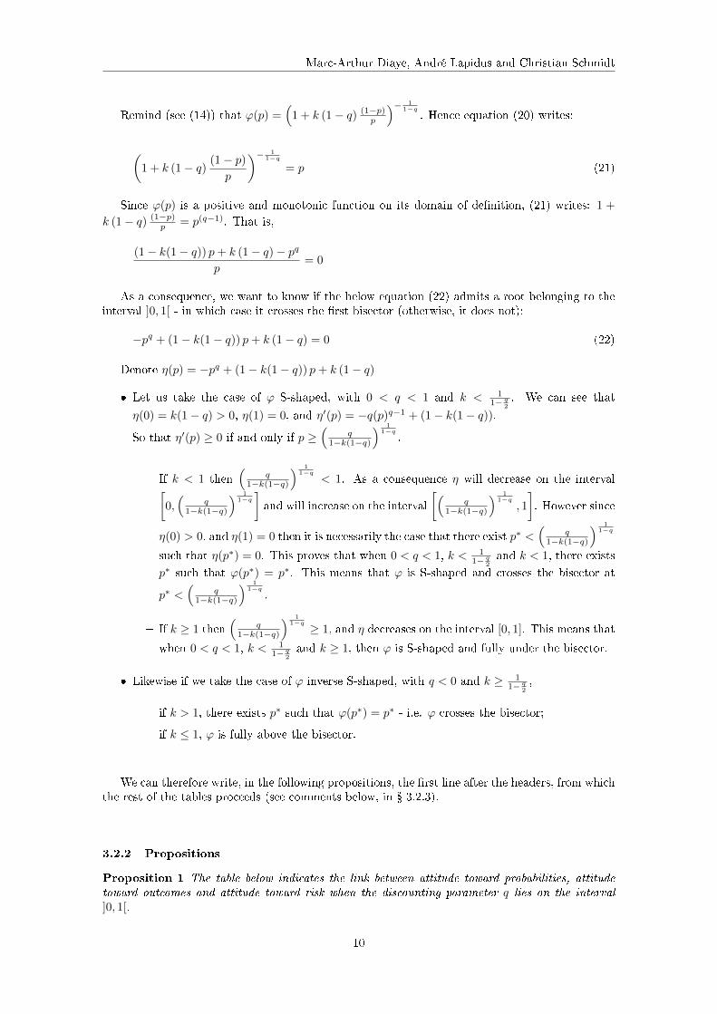
Proposition 1 The table below indicates the link between attitude toward probabilities, attitudetoward outcomes and attitude toward risk when the discounting parameter q lies on the interval]0, 1[.

10


Table 1: 0 < q < 1 - Attitudes toward probabilities, outcomes and risk

k 0 1 11− q

2+∞

ϕ S-shaped, crossing bisector S-shaped, under bisector Convex

(see Fig. 1) (see Fig. 2) (see Fig. 3)

Local Strong Pessimism Strong

Attitude toward Probability (Strong) and local Strong Optimism Pessimism

(unlikelihood insensitivity)

Attitude toward Probability (Weak) Local Weak Pessimism Weak Pessimism

and local Weak Optimism

u concave Attitude toward Neither Strong Risk Averse, Strong Risk

(decreasing sensitivity) Risk (Strong) nor Strong Risk Seeker Averse

Attitude toward Not Monotone Risk Averse Monotone Risk Averse

Risk (Monotone)

Attitude toward Not Weak Risk Averse Weak Risk Averse

Risk (Weak)

u convex Attitude toward Neither Strong Risk Averse,

(increasing sensitivity) Risk (Strong) nor Strong Risk Seeker

Attitude toward Not Monotone Risk Averse Monotone Risk Averse when Gu ≤ k

Risk (Monotone) Not Monotone Risk Averse when Gu > k

Attitude toward Not Weak Risk Averse Weak Risk Averse if

Risk (Weak) Gu ≤ k, or there exists g ≥ 1

Remarks:

• Gu = supy<x

u′(x)u′(y)

• g ≥ 1 is such that u′ (x) ≤ g u(x)−u(y)x−y , for x > y, and ϕ (p) ≤ pg

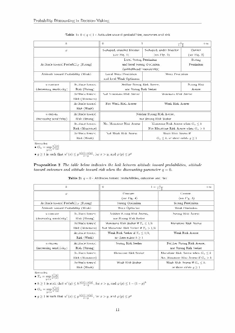
Proposition 2 The table below indicates the link between attitude toward probabilities, attitudetoward outcomes and attitude toward risk when the discounting parameter q = 0.

Table 2: q = 0 - Attitudes toward probabilities, outcomes and risk

k 0 1 = 11− q

2+∞

ϕ Concave Convex

(see Fig. 4) (see Fig. 5)

Attitude toward Probability (Strong) Strong Optimism Strong Pessimism

Attitude toward Probability (Weak) Weak Optimism Weak Pessimism

u concave Attitude toward Neither Strong Risk Averse, Strong Risk Averse

(decreasing sensitivity) Risk (Strong) nor Strong Risk Seeker

Attitude toward Monotone Risk Seeker if Tu ≤ 1/k Monotone Risk Averse

Risk (Monotone) Not Monotone Risk Seeker if Tu > 1/k

Attitude toward Weak Risk Seeker if Tu ≤ 1/k, Weak Risk Averse

Risk (Weak) or there exists h ≥ 1

u convex Attitude toward Strong Risk Seeker Neither Strong Risk Averse,


Attitude toward Monotone Risk Seeker Monotone Risk Averse when Gu ≤ k

Risk (Monotone) Not Monotone Risk Averse if Gu > k

Attitude toward Weak Risk Seeker Weak Risk Averse if Gu ≤ k,

Risk (Weak) or there exists g ≥ 1

Remarks:

• Tu = supy<x

u′(y)u′(x)

• h ≥ 1 is such that u′ (y) ≤ hu(x)−u(y)x−y , for x > y, and ϕ (p) ≤ 1− (1− p)h

• Gu = supy<x

u′(x)u′(y)

• g ≥ 1 is such that u′ (x) ≤ g u(x)−u(y)x−y , for x > y, and ϕ (p) ≤ pg

11


Proposition 3 The table below indicates the link between attitude toward probabilities, attitudetoward outcomes and attitude toward risk when the discounting parameter q is strictly negative.

Table 3: q < 0 - Attitudes toward probabilities, outcomes and risk

k 0 11− q

21 +∞

ϕ Concave Inverse S-shaped, above Inverse S-shaped, crossing

(see Fig. 6) bisector (see Fig. 7) bisector (see Fig. 8)

Local Strong Optimism

Attitude toward Probability (Strong) Strong Optimism and local Strong Pessimism

(likelihood insensitivity)

Attitude toward Probability (Weak) Weak Optimism Local Weak Optimism

and local Weak Pessimism

u concave Attitude toward Neither Strong Risk Averse,

(decreasing sensitivity) Risk (Strong) nor Strong Risk Seeker

Attitude toward Monotone Risk Seeker if Tu ≤ 1/k Not Monotone Risk Seeker

Risk (Monotone) Not Monotone Risk Seeker if Tu > 1/k

Attitude toward Weak Risk Seeker if Tu ≤ 1/k, Not Weak Risk Seeker

Risk (Weak) or there exists h ≥ 1

u convex Attitude toward Strong Risk Seeker Neither Strong Risk Averse,


Attitude toward Monotone Risk Seeker Not Monotone Risk Seeker

Risk (Monotone)

Attitude toward Weak Risk Seeker Not Weak Risk Seeker

Risk (Weak)

Remarks:• Tu = sup

y<x

u′(y)u′(x)

• h ≥ 1 is such that u′ (y) ≤ hu(x)−u(y)x−y , for x > y, and ϕ (p) ≤ 1− (1− p)h

3.2.3 Comments

a. On the attitudes toward probabilities

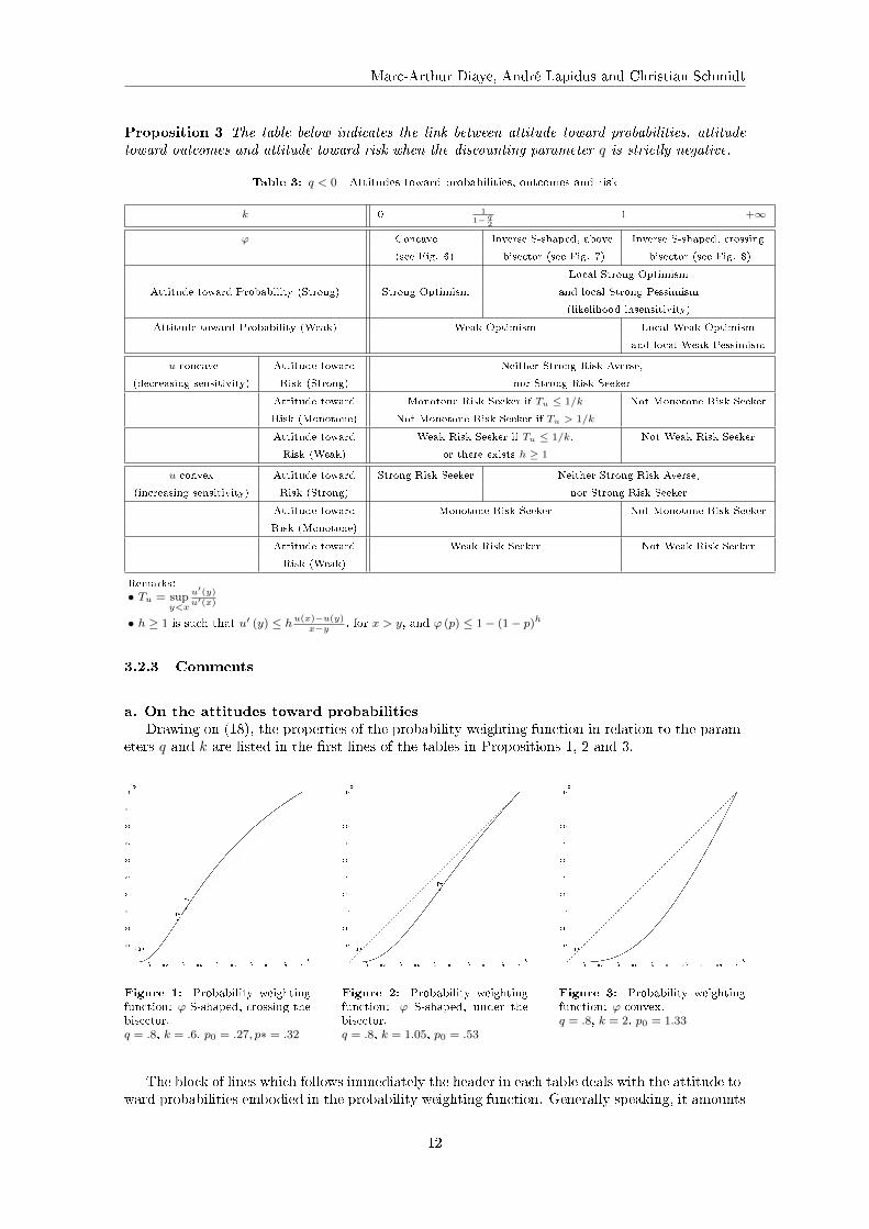
Drawing on (18), the properties of the probability weighting function in relation to the param-eters q and k are listed in the �rst lines of the tables in Propositions 1, 2 and 3.

Figure 1: Probability weightingfunction: ϕ S-shaped, crossing thebisector.q = .8, k = .6, p0 = .27, p∗ = .32

Figure 2: Probability weightingfunction: ϕ S-shaped, under thebisector.q = .8, k = 1.05, p0 = .53

Figure 3: Probability weightingfunction: ϕ convex.q = .8, k = 2, p0 = 1.33

The block of lines which follows immediately the header in each table deals with the attitude to-ward probabilities embodied in the probability weighting function. Generally speaking, it amounts

12


to pessimism or optimism, which can be approached from two di�erent points of view, each onebeing linked to a way of considering the generic term in the expression of the rank-dependentutility of a lottery: either an utility multiplied by a di�erence between transformed probabilities,or a transformed probability multiplied by a di�erence between utilities.

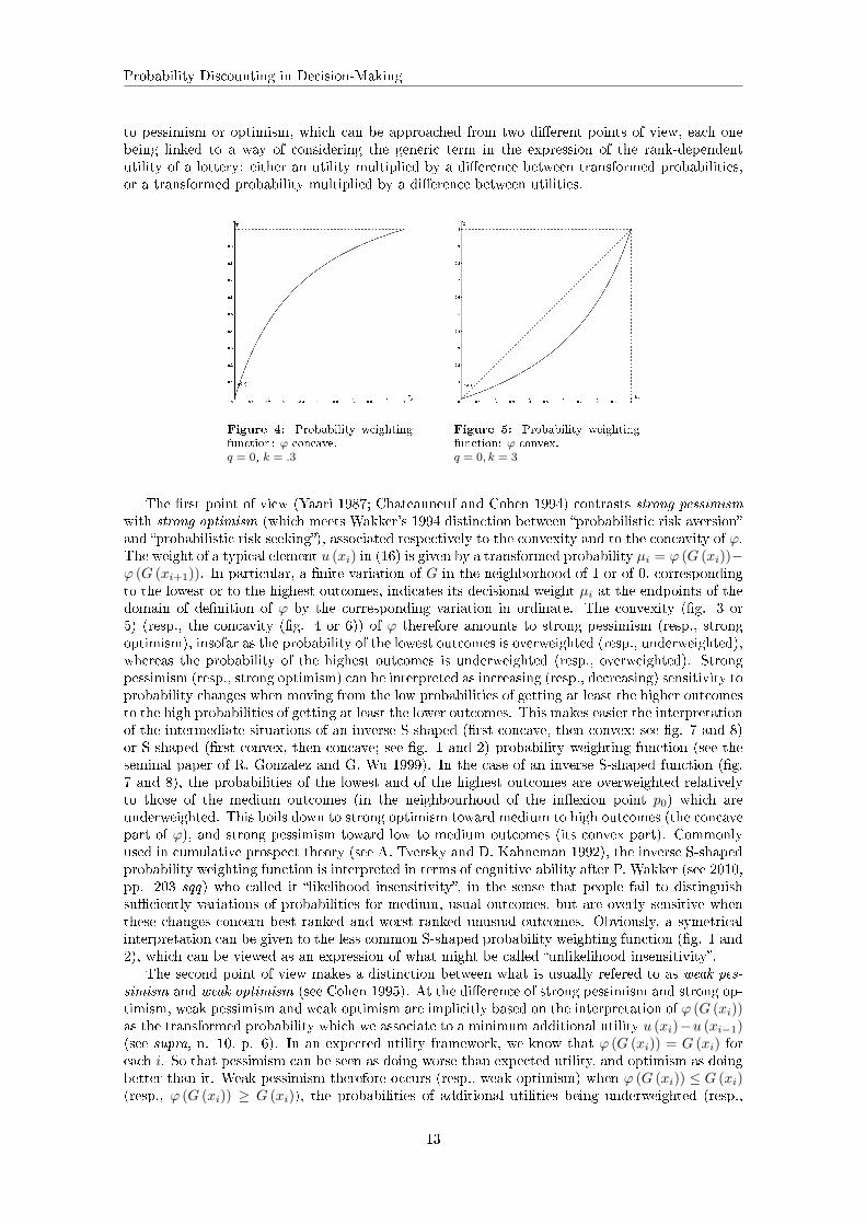
Figure 4: Probability weightingfunction: ϕ concave.q = 0, k = .3

Figure 5: Probability weightingfunction: ϕ convex.q = 0, k = 3

The �rst point of view (Yaari 1987; Chateauneuf and Cohen 1994) contrasts strong pessimismwith strong optimism (which meets Wakker's 1994 distinction between �probabilistic risk aversion�and �probabilistic risk seeking�), associated respectively to the convexity and to the concavity of ϕ.The weight of a typical element u (xi) in (16) is given by a transformed probability µi = ϕ (G (xi))−ϕ (G (xi+1)). In particular, a �nite variation of G in the neighborhood of 1 or of 0, correspondingto the lowest or to the highest outcomes, indicates its decisional weight µi at the endpoints of thedomain of de�nition of ϕ by the corresponding variation in ordinate. The convexity (�g. 3 or5) (resp., the concavity (�g. 4 or 6)) of ϕ therefore amounts to strong pessimism (resp., strongoptimism), insofar as the probability of the lowest outcomes is overweighted (resp., underweighted),whereas the probability of the highest outcomes is underweighted (resp., overweighted). Strongpessimism (resp., strong optimism) can be interpreted as increasing (resp., decreasing) sensitivity toprobability changes when moving from the low probabilities of getting at least the higher outcomesto the high probabilities of getting at least the lower outcomes. This makes easier the interpretationof the intermediate situations of an inverse S-shaped (�rst concave, then convex; see �g. 7 and 8)or S-shaped (�rst convex, then concave; see �g. 1 and 2) probability weighting function (see theseminal paper of R. Gonzalez and G. Wu 1999). In the case of an inverse S-shaped function (�g.7 and 8), the probabilities of the lowest and of the highest outcomes are overweighted relativelyto those of the medium outcomes (in the neighbourhood of the in�exion point p0) which areunderweighted. This boils down to strong optimism toward medium to high outcomes (the concavepart of ϕ), and strong pessimism toward low to medium outcomes (its convex part). Commonlyused in cumulative prospect theory (see A. Tversky and D. Kahneman 1992), the inverse S-shapedprobability weighting function is interpreted in terms of cognitive ability after P. Wakker (see 2010,pp. 203 sqq) who called it �likelihood insensitivity�, in the sense that people fail to distinguishsu�ciently variations of probabilities for medium, usual outcomes, but are overly sensitive whenthese changes concern best ranked and worst ranked unusual outcomes. Obviously, a symetricalinterpretation can be given to the less common S-shaped probability weighting function (�g. 1 and2), which can be viewed as an expression of what might be called �unlikelihood insensitivity�.

The second point of view makes a distinction between what is usually refered to as weak pes-simism and weak optimism (see Cohen 1995). At the di�erence of strong pessimism and strong op-timism, weak pessimism and weak optimism are implicitly based on the interpretation of ϕ (G (xi))as the transformed probability which we associate to a minimum additional utility u (xi)−u (xi−1)(see supra, n. 10, p. 6). In an expected utility framework, we know that ϕ (G (xi)) = G (xi) foreach i. So that pessimism can be seen as doing worse than expected utility, and optimism as doingbetter than it. Weak pessimism therefore occurs (resp., weak optimism) when ϕ (G (xi)) ≤ G (xi)(resp., ϕ (G (xi)) ≥ G (xi)), the probabilities of additional utilities being underweighted (resp.,

13


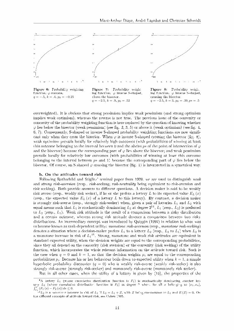
Figure 6: Probability weightingfunction: ϕ concave.q = −.5, k = .4, p0 = −0.25

Figure 7: Probability weight-ing function: ϕ inverse S-shaped,above the bisector.q = −2.5, k = .9, p0 = .52

Figure 8: Probability weight-ing function: ϕ inverse S-shaped,crossing the bisector.q = −2.5, k = 3, p0 = .39, p∗ = .5

overweighted). It is obvious that strong pessimism implies weak pessimism (and strong optimismimplies weak optimism), whereas the reverse is not true. The previous issue of the convexity orconcavity of the probability weighting function is here replaced by the question of knowing whetherϕ lies below the bisector (weak pessimism) (see �g. 2, 3, 5) or above it (weak optimism) (see �g. 4,6, 7). Consequently, S-shaped or inverse S-shaped probability weighting functions are now signi�-cant only when they cross the bisector. When ϕ is inverse S-shaped crossing the bisector (�g. 8),weak optimism prevails locally for relatively high outcomes (with probabilities of winning at leastthis outcome belonging to the interval between 0 and the abciss p∗ of the point of intersection of ϕand the bisector) because the corresponding part of ϕ lies above the bisector; and weak pessimismprevails locally for relatively low outcomes (with probabilities of winning at least this outcomebelonging to the interval between p∗ and 1) because the corresponding part of ϕ lies below thebisector. Of course, an S-shaped ϕ crossing the bisector (�g. 1) is interpreted in a symetrical way.

b. On the attitudes toward risk

Following Rothschild and Stiglitz' seminal paper from 1970, we are used to distinguish weakand strong risk-aversion (resp., risk-seeking ; risk-neutrality being equivalent to risk-aversion andrisk-seeking). Both provide answers to di�erent questions. A decision-maker is said to be weaklyrisk-averse (resp., weakly risk-seeker), if he or she prefers a lottery L to its expected value EL (x)(resp., the expected value EL (x) of a lottery L to this lottery). By contrast, a decision-makeris strongly risk-averse (resp., strongly risk-seeker) when, given a pair of lotteries L1 and L2 withequal means such that L1 is stochastically dominating L2 at degree 2

14, L1 (resp., L2) is preferredto L2 (resp., L1). Weak risk attitude is the result of a comparison between a risky distributionand a certain outcome, whereas strong risk attitude denotes a comparison between two riskydistributions. An intermediary concept was introduced by Quiggin (1992) in relation to what wasto become known as rank-dependent utility: monotone risk-aversion (resp., monotone risk-seeking)denotes a situation where a decision-maker prefers L1 to a lottery L2 (resp., L2 to L1) when L2 isa monotone increase in risk of L1

15. Strong, monotone and weak risk attitudes are equivalent instandard expected utility, when the decision weights are equal to the corresponding probabilities,since they all depend on the concavity (risk-aversion) or the convexity (risk-seeking) of the utilityfunction, which incorporates the whole relevant information on the attitude toward risk. Such isthe case when q = 0 and k = 1, so that the decision weights µi are equal to the correspondingprobabilities pi. Because his or her behaviour boils down to expected utility when k = 1, a simplehyperbolic probability discounter (q = 0) who is weakly risk-averse (weakly risk-seeker) is alsostrongly risk-averse (strongly risk-seeker) and monotonely risk-averse (monotonely risk seeker).

But in all other cases, when the utility of a lottery is given by (16), the properties of the

14A lottery L1 (whose cumulative distribution function is F1) is stochastically dominating another lot-tery L2 (whose cumulative distribution function is F2) at degree 2 when, for all x belonging to [x1, xn],∫ xx1

(F1 (s)− F2 (s)) ds ≤ 0.15L2 is a monotone increase in risk of L1 if L2 = L1 + Z, with Z being comonotone to L1 and E (Z) = 0. On

the di�erent concepts of attitude toward risk, see Cohen 1995.

14


utility function u alone are not su�cient to determine the attitude toward risk: it now dependson the properties of both the utility function u and the probability weighting function ϕ. Let ustherefore turn to the properties of the utility function. Assume, for sake of simplicity, that it isbi-di�erentiable, and either concave or convex. The concavity and the convexity of u are currentlyinterpreted as, respectively, a decreasing sensitivity and an increasing sensitivity to outcomes. Ina probability discounting framework like the one of (16), the risk attitude carried on by the utilityfunction can be either reinforced or thwarted by the attitude toward probabilities carried on bythe probability weighting function. We rely explicitly on some results concerning rank-dependentutility and adapted to q-discounting in order to account for the e�ects on risk attitude of theinteraction between the sensitivity to outcomes (u) and the attitude toward probability (ϕ).

The �rst result is from Quiggin (1992) and Cohen (1995). It shows that strong risk aversionimplies monotone risk aversion which implies weak risk aversion and, in the same way, that strongrisk seeking implies monotone risk seeking which implies weak risk seeking. The second result,from Chew, Karni and Safra (1987) states on the one hand, that decreasing sensitivity and strongpessimism is equivalent to strong risk aversion, on the other it states that increasing sensitivity andstrong optimism is equivalent to strong risk seeking. The third result is due to Chateauneuf andCohen (1994). It highlights the link between weak attitude toward risk and weak attitude towardprobability, in the sense that weak risk aversion implies weak pessimism and weak risk seekingimplies weak optimism. The fourth result is also from Chateauneuf and Cohen (1994). It aimsat �nding the extent of weak pessimism (resp., weak optimism), which can overcome increasingsensitivity (resp., decreasing sensitivity) so that weak risk aversion (resp., weak risk seeking) ismade possible. It states that whatever x, y, with x > y, whatever p ∈ [0, 1], if there exists

g ≥ 1 such that u′ (x) ≤ g u(x)−u(y)x−y and ϕ (p) ≤ pg, then weak risk aversion is satis�ed. Likewise,

whatever x, y, with x > y, whatever p ∈ [0, 1], if there exists h ≥ 1 such that u′ (y) ≤ hu(x)−u(y)x−y and

ϕ (p) ≥ 1−(1− p)h, then weak risk seeking is satis�ed. The �fth result is from Quiggin (1982, 1992;see also Chateauneuf and Cohen 1994). It says that when u is concave (resp., convex), monotonerisk aversion, weak risk aversion and weak pessimism are equivalent (respectively, monotone riskseeking, weak risk seeking and weak optimism are equivalent). Finally the last result that we useis due to Chateauneuf, Cohen, Meilijson (2005). It improves Chateauneuf and Cohen (1994) byrelying on indexes of pessimism or optimism on the one hand, and on indexes of non-concavityor non convexity of the utility function on the other hand. This result states that monotonerisk aversion is equivalent to Gu ≤ Pϕ, and monotone risk seeking is equivalent to Tu ≤ Oϕ,

where Gu = supy<x

u′(x)u′(y) is an index of non-concavity (Gu ≥ 1 and is equal to 1 when u is concave),

Tu = supy<x

u′(y)u′(x) is an index of non-convexity (Tu ≥ 1 and is equal to 1 when u is convex), Pϕ =

inf0<p<1

1−ϕ(p)ϕ(p)1−pp

≥ 1 is an index of pessimism, and Oϕ = inf0<p<1

ϕ(p)1−ϕ(p)

p1−p

an index of optimism. The result

of Chateauneuf, Cohen and Meilijson (2005) therefore expresses situations where pessimism (resp.optimism) compensates the convexity (resp. concavity) of the utility function. It can be shownthat when q-discounting occurs, Pϕ = k and Oϕ = 1/k, which are both obtained when p tends to1. So that the result of Chateauneuf, Cohen and Meilijson (2005) can be reformulated as:{

Monotone Risk Aversion⇔ Gu ≤ kMonotone Risk Seeking⇔ Tu ≤ 1/k

Drawing on the above results from the literature, it it has become possible to determine, inPropositions 1, 2 and 3, the various types of attitudes toward risk generated by the combinationbetween an attitude toward probabilities expressed by the properties of ϕ, and an attitude towardoutput which comes from the properties of u.

It is commonsense to claim that all this depends on the action of the two parameters, k and q. Inthe case of decision in time, their respective function seems rather clear (see, for instance, Takahashi2007b, pp. 639-640 and Munoz Torrecillas et al. 2018, pp. 191-192). k is usually perceivedas a parameter of �impulsivity�, which we can understand as �impatience�, since it increases thediscounting weight of physical waiting time. And q is a parameter of (time-) consistency, since whenit moves away from 1, it also makes exponential discounting more and more distant. Regarding

15


decision in risk, q separates situations of non-optimism (in which global risk-seeking of any typeis impossible) when it is greater than 0 and smaller than 1 (Proposition 1) from situations ofnon-pessimism (in which global risk-aversion, also of any type, is impossible) when it is less than0 (Proposition 3). Rather than a parameter of �risk-aversion�, as Takahashi et al. (2013, p. 877)�rst called it, k plays a crucial part as a sophisticated parameter of pessimism: it constitutes theupper-bound for the index of non-concavity Gu in order to obtain monotone risk-aversion; or itrepresents, through 1/k, the upper-bound for the index of non-convexity Tu to produce monotonerisk-seeking. This shows that appropriate values of k can compensate either the concavity orthe convexity of the utility function to produce either monotone risk-seeking in the �rst case, ormonotone risk-aversion in the second case. And if k is either too large or too small for this, itremains possible to have at least su�cient conditions to obtain weak risk-aversion or weak-riskseeking (Chateauneuf and Cohen 1994). When it is smaller than 1 (when 0 < q < 1) or greaterthan 1 (when q < 0), k generates S-shaped or inverse S-shaped probability weighting functions ϕwhich cross the bisector, so that none of the basic global attitudes toward risk can exist. In allother cases, at least weak optimism or weak pessimism occurs, so that the necessary condition forany conception of risk aversion or risk seeking is satis�ed (Chateauneuf and Cohen 1994). At last,the relation between both parameters, k and q, allows determining the range of their relative valuesfor which strong risk attitudes are possible: if q lies between 0 and 1, k ≥ 1

1− q2generates strong

pessimism, thus determining strong risk-aversion with u concave; symmetrically, if q is less than 0,k ≤ 1

1− q2generates strong optimimism, and strong risk-seeking with u convex (Chew, Karni and

Safra 1987).

4 Concluding remarks

Emerging from the intuition that probability entails a more or less long delay before winning,probability discounting has shown fruitful. Though usually avoiding the use of an explicit utilityfunction, it could integrate it and give rise to a more complete representation of risky choices.Originally presented in the framework of 2-issues lotteries, its cautiousless extension to the caseof n-issues lotteries would face the today well-known drawbacks associated to a one-to-one trans-formation of probabilities, like the violation of stochastic dominance of degree 1. This is why thesame kind of transformation as the one in use for rank-dependent utility has been employed. Thetransformation therefore concerns not a single delay or a single probability before winning, butthe average delay before obtaining at least a certain reward, or the (decumulated) probability ofgetting at least this reward. The e�ects of this transformation on the rationality of behaviour andon the attitude towards risk depend on the shape of the q-discounting function, which applies toboth time and probability.

An immediate conclusion can be drawn regarding rationality both in time and in risk. Whereasappropriate values of the parameters of the q-discounting function allow reaching the standard cri-teria of time-rationality (stationarity, through exponential discounted utility) and risk-rationality(independence, through expected utility), they cannot be ful�lled together, the latter being a par-ticular case of hyperbolic discounted utility. The attitude toward risk depends on both the attitudetoward outcomes, embedded in the utility function, and on the attitude toward probabilities ex-pressed in extended probability discounting. In a trivial way, the concavity or convexity of theutility function brings respectively risk-aversion or risk-seeking. But these have to be combinedwith the attitude toward probabilities shown by the q-discounting function in a rank-dependentutility framework. Now, according to the values of its parameters, we obtain the whole range ofthe properties of the probability weighting function usually acknowledged in the literature. Thisallows distinguishing between the di�erent types (weak and strong) of pessimism and optimismtoward probability, and to rely on the few results in the existing literature in order to determinethe various attitudes toward risk generated by the combination of a utility function and probabilitydiscounting.

Over the last thirty years or so, probability discounting has shown that in a large variety of casesit is an experimentally relevant procedure to account for behaviour under risk. From a theoreticalpoint of view, its generalisation leads to extending its scope and clarifying its meaning in terms ofrationality and attitude toward risk.

16


References

M. Abdellaoui (2009). Rank-dependent Utility, in P. Anand, P.K. Pattanaik and C. Puppe (eds),Rational and Social Choice: an Overview of New Foundations and Applications, Oxford and NewYork: Oxford University Press, pp. 69-89.

A. Chateauneuf (1999). Comonotonicity Axioms and Rank-Dependent Expected Utility Theoryfor Arbitrary Consequences, Journal of Mathematical Economics, 32, pp. 21-45.

A. Chateauneuf and M. Cohen (1994). Risk Seeking with Diminishing Marginal Utility in a Non-Expected Utility Model, Journal of Risk and Uncertainty, 9, pp. 77-91.

A. Chateauneuf, M. Cohen and I. Meilijson (2005). More Pessimism than Greediness: a Charac-terization of Monotone Risk Aversion in the Rank-Dependent Expected Utility Model, EconomicTheory, 25, pp. 649-667.

S.-H. Chew, E. Karni and Z. Safra (1987). Risk Aversion in the Theory of Expected Utility withRank Dependent Preferences, Journal of Economic Theory, 42, pp. 370-381.

M. Cohen (1995). Risk-Aversion Concepts in Expected- and Non-Expected-Utility Models, GenevaPapers on Risk and Insurance Theory, 20, pp. 73-91.

M. Cohen (2015). Risk Perception, Risk Attitude and Decision: a Rank-Dependent Approach,Mathematical Population Studies, 22(1), pp. 53-70.

S. Dehaene (2003). The Neural Basis of the Weber�Fechner Law: a Logarithmic Mental NumberLine, TRENDS in Cognitive Sciences, 7(4), pp. 145-147.

E. Diecidue and P.P. Wakker (2001). On the Intuition of Rank-Dependent Utility, Journal of Riskand Uncertainty, 23(3), pp. 281�298.

R. Gonzales and G. Wu (1999). On the Shape of the Probability Weighting Function, CognitivePsychology, 38, pp. 129-166.

L. Green and J. Myerson (2004). A Discounting Framework for Choice With Delayed and Prob-abilistic Rewards, Psychological Bulletin, 130(5), pp. 769-792.

R. Herrnstein (1981). Self-Control as Response Strength. In C.M. Bradshaw, E. Szabadi andC.F. Lowe (eds), Quanti�cation of Steady-State Operant Behavior, Amsterdam: Elsevier/North-Holland.

D. Kahneman and A. Tversky (1979). Prospect Theory: An Analysis of Decision under Risk,Econometrica, 47(2), pp. 263-291.

G. Loewenstein and D. Prelec (1992). Anomalies in Intertemporal Choice: Evidence and anInterpretation, Quarterly journal of economics, 107(2), pp. 573-597.

J.E. Mazur (1987). An Adjusting Procedure for Studying Delayed Reinforcement. In M.L. Com-mons, J.E. Mazur, J. A. Nevin, and H. Rachlin (eds.), Quantitative Analyses of Behavior (Vol. 5),The E�ect of Delay and of Intervening Events on Reinforcement Value, Hillsdale, NJ: Erlbaum,pp. 55-73.

M.J. Munoz Torrecillas, T. Takahashi, J. Gil Roales-Nieto, S. Cruz Rambaud, Z. Callejon Ruizand B. Torrecillas Jover (2018). Impatience and Inconsistency in Intertemporal Choice: An Ex-perimental Analysis, Journal of Behavioral Finance, 19(2), pp. 190-198.

P. Ostaszewski, L. Green, J. Myerson (1998). E�ects of In�ation on the Subjective Value ofDelayed and Probabilistic Rewards, Psychonomic Bulletin and Review, 5(2), pp. 324-333.

D. Prelec and G. Loewenstein (1991). Decision Making Over Time and Under Uncertainty: ACommon Approach, Management Science, 37(7), pp. 770-786.

17


J.C. Quiggin (1982). A Theory of Anticipated Utility, Journal of Economic Behavior and Orga-nization, 3, pp. 324-343.

J.C. Quiggin (1992). Increasing Risk: Another De�nition, in A. Chikan (ed.), Progress in Decision,Utility and Risk Theory, Dordrecht: Kluwer, pp. 239�248.

H. Rachlin, J. Brown and D. Cross (2000). Discounting in Judgments of Delay and Probability,Journal of Behavioral Decision Making, 13, pp. 145-159.

H. Rachlin, A.W. Logue, J. Gibbon and M. Frankel (1986). Cognition and Behavior in Studies ofChoice, Psychological Review, 93(1), pp. 33-45.

H. Rachlin, A. Raineri and D. Cross (1991). Subjective Probability and Delay, Journal of Exper-imental Analysis of Behavior, 55(2), pp. 233-244.

H. Rachlin and E. Siegel (1994). Temporal Patterning in Probabilistic Choice, OrganisationalBehavior and Decision Processes, 59, pp. 161-176.

H. Rachlin, E. Siegel and D. Cross (1994). Lotteries and the Time Horizon, Psychological Science,5(6), pp. 390-393.

M. Rothschild and J. E. Stiglitz (1970). Increasing Risk: I. A De�nition, Journal of EconomicTheory, 2, pp. 225-243.

J.B. Rotter (1954). Social Learning and Clinical Psychology, Englewood Cli�s, NJ: Prentice-Hall.

S.S. Stevens (1957). On the Psychological Law, Psychological Review, 64(3), pp. 153-181.

T. Takahashi (2005). Loss of Self-Control in Intertemporal Choice May Be Attributable to Loga-rithmic Time-Perception, Medical Hypotheses, 65, pp. 691-693.

T. Takahashi (2007a). A Probabilistic Choice Model Based on Tsallis' Statistics, Physica A:Statistical Mechanics and its Applications, 386(1), pp. 335-338.

T. Takahashi (2007b). A Comparison of Intertemporal Choices for Oneself versus Someone ElseBased on Tsallis' Statistics, Physica A: Statistical Mechanics and Its Applications, 385(2), pp.637-644.

T. Takahashi (2008). A Comparison Between Tsallis's Statistics-Based and Generalized Quasi-Hyperbolic Discount Models in Humans, Physica A: Statistical Mechanics and Its Applications,387(2-3), pp. 551-556.

T. Takahashi (2010). A Social Discounting Model Based on Tsallis' Statistics, Physica A: Statis-tical Mechanics and Its Applications, 389, pp. 3600-3603.

T. Takahashi (2011). Psychophysics of the Probability Weighting Function, Physica A: StatisticalMechanics and Its Applications, 390(5), pp. 902-905.

T. Takahashi (2013). The q-Exponential Social Discounting Functions of Gain and Loss, AppliedMathematics, 4, pp. 445-448.

T. Takahashi, R. Han, F. Nakamura (2012). Time Discounting: Psychophysics of Intertemporaland Probabilistic Choices, Journal of Behavioral Economics and Finance, 5, pp. 10-14.

T. Takahashi, R. Han, H. Nishinaka, T. Makino, H. Fukui (2013). The q-Exponential ProbabilityDiscounting of Gain and Loss, Applied Mathematics, 4, pp. 876-881.

T. Takahashi, H. Oono and M. H. B. Radford (2007). Comparison of Probabilis-tic Choice Models in Humans, Behavioral and Brain Functions, 3(20) (open access athttp://www.behavioralandbrainfunctions.com/content/3/1/20).

C. Tsallis (1994). What Are the Numbers that Experiments Provide?, Quimica Nova, 17(6), pp.468-471.

18


A. Tversky and D. Kahneman (1992). Advances in Prospect Theory: Cumulative Representationsof Uncertainty, Journal of Risk and Uncertainty, 5, pp. 297-323.

A. Tversky and P. Wakker (1995). Risk Attitudes and Decision Weights, Econometrica, 63(6), pp.1255-1280.

P.P. Wakker (1994). Separating Marginal Utility and Probabilistic Risk Aversion, Theory andDecision, 36, pp. 1-44.

P.P. Wakker (2010). Prospect Theory - For Risk and Ambiguity, Cambridge: Cambridge UniversityPress.

M.E. Yaari (1987). The Dual Theory of Choice under Risk, Econometrica, 55, pp. 95-105.

R. Yi, X. de la Piedad, W.K. Bickel (2006). The Combined E�ects of Delay and Probability inDiscounting, Behavioural Processes, 73, pp. 149-155.

19

From Decision in Risk to Decision in Time - and Return: A ...

Documents

Transcript of From Decision in Risk to Decision in Time - and Return: A ...