FROM CROWD DYNAMICS TO CROWD SAFETY: A … · September 1, 2008 19:20 WSPC/169-ACS 00185 From Crowd...
32
September 1, 2008 19:20 WSPC/169-ACS 00185 Advances in Complex Systems, Vol. 11, No. 4 (2008) 497–527 c World Scientific Publishing Company FROM CROWD DYNAMICS TO CROWD SAFETY: A VIDEO-BASED ANALYSIS ANDERS JOHANSSON and DIRK HELBING ETH Zurich, UNO D11, Universit¨ atstrasse 41, CH-8092 Zurich, Switzerland [email protected] HABIB Z. AL-ABIDEEN and SALIM AL-BOSTA Central Directorate for Holy Areas Development, Minstry of Municipal and Rural Affairs, Riyadh, Kingdom of Saudi Arabia Received 2 July 2008 Revised 5 August 2008 The study of crowd dynamics is interesting because of the various self-organization phe- nomena resulting from the interactions of many pedestrians, which may improve or obstruct their flow. Besides formation of lanes of uniform walking direction and oscilla- tions at bottlenecks at moderate densities, it was recently discovered that stop-and-go waves [D. Helbing et al., Phys. Rev. Lett. 97 (2006) 168001] and a phenomenon called “crowd turbulence” can occur at high pedestrian densities [D. Helbing et al., Phys. Rev. E 75 (2007) 046109]. Although the behavior of pedestrian crowds under extreme con- ditions is decisive for the safety of crowds during the access to or egress from mass events as well as for situations of emergency evacuation, there is still a lack of empir- ical studies of extreme crowding. Therefore, this paper discusses how one may study high-density conditions based on suitable video data. This is illustrated at the example of pilgrim flows entering the previous Jamarat Bridge in Mina, 5 kilometers from the Holy Mosque in Makkah, Saudi-Arabia. Our results reveal previously unexpected pat- tern formation phenomena and show that the average individual speed does not go to zero even at local densities of 10 persons per square meter. Since the maximum density and flow are different from measurements in other countries, this has implications for the capacity assessment and dimensioning of facilities for mass events. When conditions become congested, the flow drops significantly, which can cause stop-and-go waves and a further increase of the density until critical crowd conditions are reached. Then, “crowd turbulence” sets in, which may trigger crowd disasters. For this reason, it is important to operate pedestrian facilities sufficiently below their maximum capacity and to take measures to improve crowd safety, some of which are discussed in the end. Keywords : Pedestrian dynamics; crowd turbulence; video analysis; fundamental diagram. 1. Introduction It is well-known that driven many-particle systems often constitute complex sys- tems, in which different kinds of pattern formation phenomena are observed [4]. 497
Transcript of FROM CROWD DYNAMICS TO CROWD SAFETY: A … · September 1, 2008 19:20 WSPC/169-ACS 00185 From Crowd...

September 1, 2008 19:20 WSPC/169-ACS 00185
Advances in Complex Systems, Vol. 11, No. 4 (2008) 497–527c© World Scientific Publishing Company
FROM CROWD DYNAMICS TO CROWD SAFETY:A VIDEO-BASED ANALYSIS
ANDERS JOHANSSON and DIRK HELBING
ETH Zurich, UNO D11, Universitatstrasse 41,CH-8092 Zurich, Switzerland
HABIB Z. AL-ABIDEEN and SALIM AL-BOSTA
Central Directorate for Holy Areas Development,Minstry of Municipal and Rural Affairs,
Riyadh, Kingdom of Saudi Arabia
Received 2 July 2008Revised 5 August 2008
The study of crowd dynamics is interesting because of the various self-organization phe-nomena resulting from the interactions of many pedestrians, which may improve orobstruct their flow. Besides formation of lanes of uniform walking direction and oscilla-tions at bottlenecks at moderate densities, it was recently discovered that stop-and-gowaves [D. Helbing et al., Phys. Rev. Lett. 97 (2006) 168001] and a phenomenon called“crowd turbulence” can occur at high pedestrian densities [D. Helbing et al., Phys. Rev.E 75 (2007) 046109]. Although the behavior of pedestrian crowds under extreme con-ditions is decisive for the safety of crowds during the access to or egress from massevents as well as for situations of emergency evacuation, there is still a lack of empir-ical studies of extreme crowding. Therefore, this paper discusses how one may studyhigh-density conditions based on suitable video data. This is illustrated at the exampleof pilgrim flows entering the previous Jamarat Bridge in Mina, 5 kilometers from theHoly Mosque in Makkah, Saudi-Arabia. Our results reveal previously unexpected pat-tern formation phenomena and show that the average individual speed does not go tozero even at local densities of 10 persons per square meter. Since the maximum densityand flow are different from measurements in other countries, this has implications forthe capacity assessment and dimensioning of facilities for mass events. When conditionsbecome congested, the flow drops significantly, which can cause stop-and-go waves and afurther increase of the density until critical crowd conditions are reached. Then, “crowdturbulence” sets in, which may trigger crowd disasters. For this reason, it is importantto operate pedestrian facilities sufficiently below their maximum capacity and to takemeasures to improve crowd safety, some of which are discussed in the end.
Keywords: Pedestrian dynamics; crowd turbulence; video analysis; fundamental diagram.
1. Introduction
It is well-known that driven many-particle systems often constitute complex sys-tems, in which different kinds of pattern formation phenomena are observed [4].
497

September 1, 2008 19:20 WSPC/169-ACS 00185
498 A. Johansson et al.
Depending on certain system parameters (the “order parameters”), one may findtransitions from one state of collective behavior to a qualitatively different behav-ior [8]. Such transitions typically occur when a certain “critical threshold” is crossed.It is interesting to study, whether such transitions can also be found in systemsinvolving humans [12, 36]. In this case, the role of particles is replaced by individ-uals, which follow different interaction rules. Nevertheless, it has been shown thatmany stylized facts of pedestrian crowds can be well understood by so-called “socialforce models” [14] and other modeling approaches such as cellular automata [1,23].As examples we mention the segregration of different walking directions into laneswith a uniform direction of motion, or oscillations of the passing direction at bot-tlenecks [19]. Recently, we have observed two unexpected transitions in extremelydense pedestrian crowds [17]. While we found laminar flows at small and mod-erate densities, there was a sudden onset of stop-and-go waves, which was laterreplaced by a phenomenon of highly irregular motion called “crowd turbulence”.This dynamics is dangerous, as it may cause people to fall, and it seems to be relatedwith coordination problems between neighboring pedestrians competing for littlespace. Both, stop-and-go waves and crowd turbulence were previously not expected,because the acceleration time of pedestrians is only about 0.5 seconds [28], whichsuggests a quasi-adiabatic relaxation to a stationary state characterized by the“fundamental diagram”, i.e. a flow–density relationship. In contrast, stop-and-gowaves in freeway traffic are caused by significant delays in the speed adjustmentsof vehicles [13].
The study of dense pedestrian crowds is particularly interesting, since it is oneof few systems involving a large numbers of humans (up to millions), where thedetailed dynamics can still be revealed by analyzing empirical data [17] or perform-ing agent-based simulations [43]. Particularly intensive research activities have beentriggered by the study of stampedes [16]. While “panic” has recently been studiedin animal experiments with mice [34] and ants [3] there is still an evident lack ofdata on critical conditions in human crowds. Recent work [35, 44] goes into thedirection of comparing empirical studies with each other, and bringing consensusto some of the fundamental issues in evacuation dynamics.
However, for a long time, unidirectional pedestrian flows were predominantlyassumed to move smoothly according to the “fluid-dynamic” flow–density relation-ship [41]:
Q(ρ) = ρV (ρ), (1)
where Q represents the flow per meter width, ρ is the pedestrian density, and theaverage velocity V is believed to go to zero at some maximum density as in trafficjams [5,27,32,33,37,41]. Formula (1) is often used as a basis for dimensioning anddesigning pedestrian facilities, for safety and evacuation studies. However, empir-ical measurements are often restricted to densities up to 4–6 persons/m2. In thestudy [41], for example, the maximum density ρmax is 5.4 persons/m2, and the

September 1, 2008 19:20 WSPC/169-ACS 00185
From Crowd Dynamics to Crowd Safety 499
corresponding fit curve of the speed–density relationship is
V (ρ) = V0
{1 − exp
[−a
(1ρ− 1
ρmax
)]}, (2)
where V0 = 1.34 m/s is the free speed at low densities and a = 1.913 personsper square meter a fit parameter. Some other measurements of pedestrian densi-ties, however, reach upto 6 persons per square meter or more [27, 33]. So, whichmeasurement is correct? And what happens at even higher densities? Based onthe projected area of human bodies, upto 11 persons may fit into one squaremeter [38].
In order to address these issues, we will evaluate video recordings of the annualMuslim pilgrimage, where conditions are known to be particularly crowded. Wewill also see that these data are not directly transferable to Western European con-ditions and vice versa. Video-based studies of pedestrian flows have recently beencarried out by other authors as well [20, 26, 37]. Most of them focus on bottleneckrather than unconstrained flows. Helbing et al. [18] have recently proposed a macro-scopic model for such flows. The situation we analyze in the following, however, ischaracterized by particularly extreme densities, which have finally led to the crowddisaster on January 12, 2006. Therefore, we expect particular insights into criticalcrowd conditions.
Our paper intends to identify some reasons for the different flow–density curves(fundamental diagrams) reported in the literature and to close the data gap in thesafety-relevant range of extreme densities. Considering the inconsistent measure-ments in the literature, which one should a capacity analysis be based on? Usingthe wrong curves can easily imply a wrong dimensioning and, thereby, future disas-ters. Generally, the difference between local and global measurements has not beensufficiently paid attention to. The same applies to the body size distribution andthe cultural backgrounds (regardings prefered spacing and speeds). Many papersalso do not present standard deviations, which are important to judge the variabil-ity of the measurement points, to compare different data sets and to determine therequired capacity reserves when planning pedestrian facilities.
The technique of video analysis is an important, but not the main point ofour paper. Nevertheless, we show in detail how certain problems related to video-based evaluations can be successfully overcome and how the results depend on thespecification of parameters. Note that the video-based evaluation method describedin this paper was also used for another study [17]. While that study focused onthe dynamics of crowd disasters, this paper addresses the measurement processand safety-relevant features of the speed–density and flow–density diagrams. Theseissues are important to draw correct conclusions from the video data. Another focusis the determination of critical crowd conditions. It will turn out that neither thedensity nor the speed or flow field are good measures of the criticality in the crowd,as the latter actually depends on the crowd dynamics.

September 1, 2008 19:20 WSPC/169-ACS 00185
500 A. Johansson et al.
The remainder of this paper describes the large efforts and various difficultiesthat must be overcome in order to extract the characteristics and dynamics ofcrowd behavior at large densities from video recordings. As commercial trackingsoftware did not do the job, we had to develop new algorithms which were capableof dealing with hundreds rather than dozens of people in a fully automated way.This involved the evaluation of terabytes of data, recorded at many measurementsites over several days in January 2006 (during the Hajj of the year 1426H). Thewhole project, including the comparison with manual counts for validation andcalibration of the method required several man years.
Our paper is structured as follows: Section 2 will describe our technique of videoevaluation, which is the basis of our data analysis. In Sec. 3 we will then definea new measurement method for local densities and flows. Problems like how tocorrect for the hiding of people by umbrellas will be addressed as well. Afterwards,Sec. 4 will present empirical measurement results for the flow–density and speed–density diagrams at the entrance of the previous Jamarat Bridge. Here, we willalso study the considerable variability of density, velocity and flow data. In Sec. 5we will describe the stop-and-go waves and the phenomenon of “crowd turbulence”discovered at high densities. Moreover, we will determine warning signs of criticalcrowd conditions, in particular the “crowd pressure”. Section 6 will summarizeour results and discuss implications for the safety analysis and dimensioning ofpedestrian facilities.
2. Measurement Site and Video Tracking
2.1. Description of measurement site and conditions
In order to get a better understanding of extremely dense conditions, we havescientifically evaluated the situation during the stoning ritual in Mina through 12fixed cameras mounted on high poles. The overall video material of the 10th to 12thday of Dhu al-Hijjah, 1426H amounts to more than 2 Terabyte of data. A specialfocus of the study presented here will be on the entrance area of the Jamarat Bridge(see Fig. 1), where the situation became particularly crowded and the sad crowddisaster happened on January 12, 2006 (the 12th day of the pilgrimage).
2.2. Video tracking method
Video tracking has become a common and comfortable tool for empirical pedes-trian research recently [21, 25, 39]. Its big advantage is the automatic evaluation ofpedestrian trajectories, but video tracking has also its limitations:
• Some tracking software packages require to specify the starting points of pedes-trians manually by clicking on their heads.
• Possible camera positions often imply small areas of recording or oblique camerapositions. The latter implies that pedestrians may be hidden behind each otherat high densities. In both cases, one must correct for effects of perspective.

September 1, 2008 19:20 WSPC/169-ACS 00185
From Crowd Dynamics to Crowd Safety 501
Fig. 1. Illustration of the old Jamarat Bridge and the video-recorded area we are concentratingon in this study. There were many more cameras installed, but the one in the entrance area showedthe highest densities and the most interesting crowd dynamics.
• In dense pedestrian crowds, pedestrians are often “lost” or interchanged by thetracking algorithm.
• Most tracking algorithms are restricted to tracking several dozens of pedestriansfor the above reasons and reasons of numerical performance.
Thanks to the 35 meter high pole at which our video camera was mounted, therecorded area was quite large (28m× 23m) and the recordings could be madealmost perpendicular to the ground. Therefore, pedestrians of different height wereusually not hidden behind each other. However, the radius of a pedestrian headextended over 2–3 pixels only (corresponding to about 15–25 pixels covered by eachhead).
The software developed by the authors automatically determines heads bysearching for round structures. For this purpose, several digital filters (transfor-mations) are successively applied to the video frames to enhance their contrast andidentify the relevant structures (see Fig. 2). To gain a higher accuracy, the followingadditional steps are performed:
• Double-checking of the identified circles by applying an Artificial Neural Network[24] trained to recognize heads.
• Application of adaptive histogram equalization to compensate for variations inthe light conditions.
• Application of corrections derived from extensive manual count data (see Fig. 3and Sec. 2.2.1).
Figure 4 illustrates how the video frames look like during several processing stepsof the tracking algorithm.
For each frame, the identification of heads yields the locations �ri(t) of the pedes-trians i at time t. By comparing these with their local neighborhoods in the nextvideo frame, one can determine their velocities �vi(t). The speed information is usedto estimate the location of the pedestrians in the subsequent frame, which improves

September 1, 2008 19:20 WSPC/169-ACS 00185
502 A. Johansson et al.
Fig. 2. Illustration of how the video-analysis software operates. The raw video data are fed fromthe top, and each frame is passing a number of filters (actually more than shown over here), untilthe head locations and velocities are obtained with sufficient reliability in the end.
(a) (b)
Fig. 3. (a) Part of a video frame used for manual counting and calibration; (b) schematic illus-tration of the method used for the manual counting of pedestrians. The crowd video is playedfor 5 seconds in slow-motion at 1/10th of the original speed, and two people are independentlycounting the number of pedestrians who cross a certain line within these 5 seconds. The countingis not done for the complete video recording, but for short video sequences separated by timeintervals of 10 minutes each.

September 1, 2008 19:20 WSPC/169-ACS 00185
From Crowd Dynamics to Crowd Safety 503
(a) (b)
(c) (d)
Fig. 4. Illustration of video frames before and after certain transformations performed by ourvideo analysis software. (a) Original frame; (b) same frame, after the lense distortion was correctedfor (see the straightened wall in the lower part.); (c) the frame after edge detection and thresholdingwere applied; (d) frame superposed to the head-detection probability-density surface, with crosseson the most likely head locations as determined by an Artificial Neural Network (ANN) [24].The probability density is determined by searching for head-like patterns in the current frame aswell as extrapolating the locations of head detections made in previous frames, which results in areinforcement when the same head is detected in many consecutive frames. A cross is displayedif the probability density is above a certain threshold and there is no more likely head locationwithin a distance corresponding to one head diameter. The inaccuracies in the upper left cornerare both due to the fact that the video is blurry in this region, but also because these pedestrianshave just entered the video and therefore the reinforcement of the tracking algorithm has not yettaken effect.
the accuracy of the tracking procedure. With a resolution of 25 pixels per meterand 8 frames per second, it is possible to determine even small average speeds bycalculating the mean value over a large enough sample of individual speed mea-surements.

September 1, 2008 19:20 WSPC/169-ACS 00185
504 A. Johansson et al.
0
2
4
6
8
10
0 10 20 30 40 50 60 70 80
Flo
w (
pers
ons/
s)
Time (h)
Automatic countManual count
0
100000
200000
300000
400000
500000
600000
700000
800000
0 10 20 30 40 50 60 70 80N
(pe
rson
s)Time (h)
Automatic countManual count
(a) (b)
0
2
4
6
8
10
0 10 20 30 40 50 60 70 80
Flo
w (
pers
ons/
s)
Time (h)
Automatic countManual count
0
100000
200000
300000
400000
500000
600000
700000
800000
0 10 20 30 40 50 60 70 80
N (
pers
ons)
Time (h)
Automatic countManual count
(c) (d)
Fig. 5. Flow and cumulative flow of a pedestrian road to the Jamarat plaza over 72 hours.(a, b): Comparison of automatically and manually determined values, using the methods illustratedin Figs. 2 and 3. (c, d): Same comparison, when more sophisticated classifiers based on ArtificialNeural Networks [24] were used.
2.2.1. Comparison of automated and manual counts
The tracking routine does not only give good estimates of the local densities, speedsand flows. It is also suitable for counting people. Figure 5 compares automated andmanual counts for one street leading to the Jamarat Plaza. Despite the difficultyto distinguish people walking in opposite directions, the reliability of the auto-mated counts is reasonably high. The deviation is actually of the same order as thedeviation between manual counts of two different persons.
3. Measurement of Local Densities, Speeds, and Flows
3.1. Data evaluation method
From the locations �ri(t) of the pedestrians i at time t, we have determined the localdensity ρ(�r, t) = ρR
t (�r ) at a location �r via the formula
ρ(�r, t) = ρRt (�r ) =
1πR2
∑j
exp[−‖�rj(t) − �r‖2/R2], (3)
September 1, 2008 19:20 WSPC/169-ACS 00185
From Crowd Dynamics to Crowd Safety 505
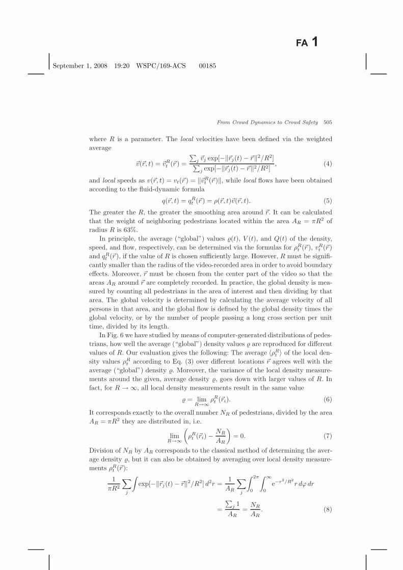
where R is a parameter. The local velocities have been defined via the weightedaverage
�v(�r, t) = �vRt (�r ) =
∑j �vj exp[−‖�rj(t) − �r‖2/R2]∑
j exp[−‖�rj(t) − �r‖2/R2], (4)
and local speeds as v(�r, t) = vt(�r ) = ‖�vRt (�r )‖, while local flows have been obtained
according to the fluid-dynamic formula
q(�r, t) = qRt (�r ) = ρ(�r, t)�v(�r, t). (5)
The greater the R, the greater the smoothing area around �r. It can be calculatedthat the weight of neighboring pedestrians located within the area AR = πR2 ofradius R is 63%.
In principle, the average (“global”) values �(t), V (t), and Q(t) of the density,speed, and flow, respectively, can be determined via the formulas for ρR
t (�r ), vRt (�r )
and qRt (�r ), if the value of R is chosen sufficiently large. However, R must be signifi-
cantly smaller than the radius of the video-recorded area in order to avoid boundaryeffects. Moreover, �r must be chosen from the center part of the video so that theareas AR around �r are completely recorded. In practice, the global density is mea-sured by counting all pedestrians in the area of interest and then dividing by thatarea. The global velocity is determined by calculating the average velocity of allpersons in that area, and the global flow is defined by the global density times theglobal velocity, or by the number of people passing a long cross section per unittime, divided by its length.
In Fig. 6 we have studied by means of computer-generated distributions of pedes-trians, how well the average (“global”) density values � are reproduced for differentvalues of R. Our evaluation gives the following: The average 〈ρR
t 〉 of the local den-sity values ρR
t according to Eq. (3) over different locations �r agrees well with theaverage (“global”) density �. Moreover, the variance of the local density measure-ments around the given, average density �, goes down with larger values of R. Infact, for R → ∞, all local density measurements result in the same value
� = limR→∞
ρRt (�ri). (6)
It corresponds exactly to the overall number NR of pedestrians, divided by the areaAR = πR2 they are distributed in, i.e.
limR→∞
(ρR
t (�ri) −NR
AR
)= 0. (7)
Division of NR by AR corresponds to the classical method of determining the aver-age density �, but it can also be obtained by averaging over local density measure-ments ρR
t (�r ):
1πR2
∑j
∫exp[−‖�rj(t) − �r‖2/R2] d2r =
1AR
∑j
∫ 2π
0
∫ ∞
0
e−r2/R2r dϕ dr
=
∑j 1
AR=
NR
AR. (8)

September 1, 2008 19:20 WSPC/169-ACS 00185
506 A. Johansson et al.
0 2 4 6 8 10 120
2
4
6
8
10
12
Global density
Loca
l den
sity
, ρ
Uniform distributionR=1
0 2 4 6 8 10 120
2
4
6
8
10
12
Global density
Loca
l den
sity
, ρ
Uniform distributionR=3
(a) (b)
0 2 4 6 8 10 120
2
4
6
8
10
12
Global density
Loca
l den
sity
, ρ
Simulated distributionR=1
0 2 4 6 8 10 120
2
4
6
8
10
12
Global density
Loca
l den
sity
, ρ
Hexagonal-grid distributionR=1
(c) (d)
Fig. 6. Local density measurements according to formula (3) for 10 randomly picked points in acircle of 10 meter radius, compared to the average density in a circular area AR of radius R = 100meters. Uniformly distributed points with R = 1 (a) and R = 3 (b). Note that the local densityof randomly distributed points varies strongly, as different points can be arbitrarily close to eachother. Therefore, we also generated pedestrian distributions resulting from a pedestrian simulationwith the social force model [14], which took into account the finite space requirements (“diame-ters”) of pedestrians. In this simulation, we assumed an average desired velocity of 1.34 metersper second and a standard deviation of 0.26 meters per second as in Ref. 41. The desired directionof walking were assumed to be the same for all pedestrians. The initial distribution was randomlychosen, but the density measurement was made after a simulated time of 30 seconds. The result-ing density distribution for R = 1 (c) is significantly smaller, as the distribution of pedestrians ismore regular than a random distribution due to their repulsive interactions. To a certain extent,it reminds of the distribution of points located on a hexagonal lattice ((d) for R = 1).
Note, however, that we are not so much interested here in the average density �,but in the local density ρ(�ri, t), as this is expected to determine the behavior ofpedestrian i. The variation of the values of ρi(�r, t) in Fig. 6 is due to the statisticalvariation of pedestrians in space, which results in local density variations. If thevalue of R is fixed, the relative variation of measured density values is smaller forhigher densities, due to the larger number of pedestrians in the area NR = πR2.
September 1, 2008 19:20 WSPC/169-ACS 00185
From Crowd Dynamics to Crowd Safety 507
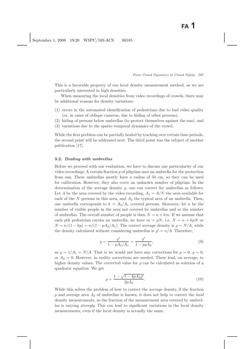
This is a favorable property of our local density measurement method, as we areparticularly interested in high densities.
When measuring the local densities from video recordings of crowds, there maybe additional reasons for density variations:
(1) errors in the automated identification of pedestrians due to bad video quality(or, in cases of oblique cameras, due to hiding of other persons),
(2) hiding of persons below umbrellas (to protect themselves against the sun), and(3) variations due to the spatio–temporal dynamics of the crowd.
While the first problem can be partially healed by tracking over certain time periods,the second point will be addressed next. The third point was the subject of anotherpublication [17].
3.2. Dealing with umbrellas
Before we proceed with our evaluation, we have to discuss one particularity of ourvideo recordings: A certain fraction p of pilgrims uses an umbrella for the protectionfrom sun. These umbrellas mostly have a radius of 50 cm, so they can be usedfor calibration. However, they also cover an unknown number of pilgrims. In thedetermination of the average density �, one can correct for umbrellas as follows:Let A be the area covered by the video recording, A1 = A/N the area available foreach of the N persons in this area, and A2 the typical area of an umbrella. Then,one umbrella corresponds to k = A2/A1 covered persons. Moreover, let n be thenumber of visible people in the area not covered by umbrellas and m the numberof umbrellas. The overall number of people is then N = n + km. If we assume thateach pth pedestrian carries an umbrella, we have m = pN , i.e. N = n + kpN orN = n/(1 − kp) = n/(1 − pA2/A1). The correct average density is � = N/A, whilethe density calculated without considering umbrellas is �′ = n/A. Therefore,
� =�′
1 − pA2/A1=
�′
1 − p�A2, (9)
as � = 1/A1 = N/A. That is we would not have any corrections for p = 0, � = 0,or A2 = 0. However, in reality corrections are needed. These lead, on average, tohigher density values. The corrected value for � can be calculated as solution of aquadratic equation. We get
� =1 −
√1 − 4pA2�′
2pA2. (10)
While this solves the problem of how to correct the average density, if the fractionp and average area A2 of umbrellas is known, it does not help to correct the localdensity measurements, as the fraction of the measurement area covered by umbrel-las is varying strongly. This can lead to significant variations in the local densitymeasurements, even if the local density is actually the same.

September 1, 2008 19:20 WSPC/169-ACS 00185
508 A. Johansson et al.
For that reason, within a 20m× 15m area, we have randomly picked pedestrianlocations and have determined the local densities around them. From this sample,we have removed the fraction γ of lowest density values. Since the umbrellas aremost likely to be found in the low-density regime, the probability of successfullyfiltering out umbrellas grows with γ. Note that we do not assume that personswith umbrellas tend to avoid large densities. Rather the idea is that the densitycalculation underestimates the density in the vicinity of an umbrella because thesurrounding persons are hidden under the umbrella. Figure 7 shows the computer-generated data that filtering out 50% of the low-density data can still lead tosignificant underestimation of the actual density by the measured one, while γ =0.95 leads to reasonably accurate density measurements. Therefore, in the followingempirical evaluations of video-recorded pilgrim flows, we will restrict to sufficientlyreliable measurements of local densities by using a cutoff value of γ = 0.95.
Let us now check the plausibility of the above proposed methods to correctfor umbrellas with real data. In order to investigate how the speed–density andflow–density diagrams depend on the cutoff value γ, we have evaluated them fordifferent values of γ (see Fig. 8). We find that, while the speed–density relationshipsvary relatively little with the variation of γ, there is a significant increase of thelocal flows for greater γ values, particularly in the intermediate density range. Thisshows that fitting speed–density data may lead to unreliable conclusions regardingthe flow–density relationship, while fitting flow–density data would lead to good
0 2 4 6 8 100
2
4
6
8
10
Actual local density (persons/m2)
Mea
sure
d lo
cal d
ensi
ty (
pers
./m2 )
0 2 4 6 8 100
2
4
6
8
10
Actual local density (persons/m2)
Mea
sure
d lo
cal d
ensi
ty (
pers
./m2 )
(a) (b)
Fig. 7. Simulated results to determine the influence of umbrellas on the local density measure-ments. The computer simulations have been carried out with the social force model, starting
with random initial conditions. We have assumed that 2% of the persons carry umbrellas witha radius of 50 cm. While the actual local density has been determined from all generated points(representing pedestrians), the measured local density has been determined by removing all pointsin a radius of 50 cm around 2% of the points. The figures show the measured over the actuallocal density for a cutoff of (a) γ = 0.5 and (b) γ = 0.95. A cutoff value of γ = 0.95 reproduceslocal density measurements over a large range of densities well, while a cutoff of γ = 0.5 tends tounderestimate the actual local densities.

September 1, 2008 19:20 WSPC/169-ACS 00185
From Crowd Dynamics to Crowd Safety 509
0 2 4 6 8 100
0.5
1
1.5
2
Local density (1/m2)
Loca
l spe
ed (
m/s
)
Increasing γ
0 2 4 6 8 100
0.5
1
1.5
2
Local density (1/m2)Lo
cal f
low
(1/
m/s
) Increasing γ
(a) (b)
Fig. 8. Empirical relationships between (a) the local speed and the local density and between (b)the local flow and the local density for the measurement site depicted in Fig. 1 and various valuesof γ ∈ {0%, 25%, 50%, 75%, 95%}. The cutoff value γ is supposed to correct for the influence ofumbrellas. It is clear that the flow values are underestimated if pedestrians covered by umbrellasare not suitably accounted for, as for small values of γ.
0 2 4 6 8 100
0.5
1
1.5
2
Global density (1/m2)
Glo
bal s
peed
(m
/s)
Increasing p
0 2 4 6 8 100
0.5
1
1.5
2
Global density (1/m2)
Glo
bal f
low
(1/
m/s
)
Increasing p
(a) (b)
Fig. 9. Relationships between (a) the globally averaged speed and the global density andbetween (b) the globally averaged flow and the global density for various values of p ∈{0%, 1%, 2%, . . . , 6%}, using formula (10). As a larger assumed fraction p of umbrellas impliesa larger number of hidden pedestrians, it is clear that the flow must increase with the valueof p.
velocity–density fits as well. The reason is that the density enters twice and in amultiplicative manner into the flow (as product of density and speed).
Moreover, we have determined the globally averaged speed and the global flowas a function of the global density for different assumed fractions of umbrellas p
(see Fig. 9).Let us now address the question, how the actual fraction of umbrellas can
be determined from the video recordings. For this, we used the fact that therelationship between the local speed and the local density should not be changedsignificantly by the fraction p of umbrellas. We, therefore, defined a reference

September 1, 2008 19:20 WSPC/169-ACS 00185
510 A. Johansson et al.
relationship ρref(v), measured the velocity v and density ρ, and calculated the frac-tion p of umbrellas that leads to consistent density values. In detail, the procedurewas as follows:
• As a reference relationship ρref(v), we used a fit curve to data of the local densityas a function of the local speed, determined for R = 1 and γ = 95%. Accordingto our previous numerical studies, the large cutoff value γ should eliminate theinfluence of umbrellas well.
• At a given time point t, we picked 1000 random locations �ri.• For these locations, we determined the local densities ρ′|γ=0(�ri) and the local
speeds v|γ=0(�ri) with R = 1m and γ = 0. The value γ = 0 ignored umbrellasand resulted in density values ρ′ ≤ ρ, but the speeds should be correct.
• We then estimated the corrected densities as ρ(�ri) = ρref
(v|γ=0(�ri)
).
• Next, we determined the global density �(t) as average of the corrected localdensities ρ(�ri), i.e. �(t) = 〈ρ(�ri)〉. Similarly, we obtained the global density �′(t)ignoring umbrellas as average of the densities ρ′|γ=0(�ri), i.e. �′(t) = 〈ρ′|γ=0(�ri)〉.
• Finally, we estimated the fraction of umbrellas via the formula
p(t) =�(t) − �′(t)
�2(t)A2, (11)
which follows from Eq. (9). As the radius of most umbrellas was 0.5m, we usedthe value A2 = π0.52 m2.
The empirically determined fraction p(t) of umbrellas as function of time t is shownin Fig. 10. It turns out that the fraction of umbrellas increases after 10:30 am andreaches its maximum at noon time, when the sunshine is strongest. This shows theplausibility of our procedure, which has also been checked by manual counts.
10 10.5 11 11.5 12 12.50
1
2
3
4
Time (h)
Fra
ctio
n of
um
brel
las,
p (
%)
Fig. 10. Fraction p of pilgrims carrying umbrellas as a function of time. One can see that p isfour times larger around noon time, as compared to an hour earlier.

September 1, 2008 19:20 WSPC/169-ACS 00185
From Crowd Dynamics to Crowd Safety 511
0 2 4 6 8 100
0.2
0.4
0.6
0.8
Local density (persons/m2)
Den
sity
dis
trib
utio
n
Fig. 11. Distribution of local densities (with R = 1) for a given average density (circles:1.6 persons/m2, crosses: 3.0 persons/m2, dots: 5.0 persons/m2). Gamma distributions fit thehistograms with 50 bins well (solid lines), after Ref. 17.
4. Empirical Findings
After the previous description of our video evaluation procedure, let us now startour analysis of pedestrian recordings with a discussion of density measurements.Figure 11 shows that there is always a large variation of local densities, and thisvariation is very important, as the safety in a crowd is not determined by theaverage density, but by the maximum occuring density. One can roughly say thatthe maximum densities are twice as high as the average density. Therefore, anaverage density of 4 persons/m2 should not be exceeded [38].
4.1. Relationships between densities, velocities and flows
In this section we are mainly interested in local crowd conditions, as they arerelevant for the criticality in the crowd. Let us first give empirical results for thedependence of the locally averaged speed v(�r, t) = vR
t (�r ) and the locally averagedflow q(�r, t) = qR
t (�r ) on the local density ρ(�r, t) = ρRt (�r ) (see Fig. 12). We find
that, with larger averaging radius R, the maximum densities and flows are reduced.This is due to the considerable variation of the local density, speed and flow values.In Fig. 12, we have therefore also determined the density and flow values witha variable radius R =
√10/�, in order to average over a comparable number of
pedestrians in all density ranges.An important observation is the fact that the average local speed at the entrance
to the Jamarat Bridge does not become zero even at local densities of 10 persons persquare meter. This, of course, does not mean that pedestrians never stop, but thatstops last for short time periods only [17]. The observation of non-vanishing speedsat extreme local densities is in marked contrast to vehicle traffic, where driversstop and keep enough distance to avoid collisions. The consequence of this pedes-trian behavior is that their average flows remain finite, with short interruptions

September 1, 2008 19:20 WSPC/169-ACS 00185
512 A. Johansson et al.
0 2 4 6 8 100
0.5
1
1.5
2
Local density (1/m2)
Loca
l spe
ed (
m/s
) R=1R=2R= 10/ρ
0 2 4 6 8 100
0.5
1
1.5
2
Local density (1/m2)Lo
cal f
low
(1/
m/s
)
R=1R=2R= 10/ρ
(a) (b)
Fig. 12. Average local (a) speed and (b) flow as a function of the local density ρ. The unexpectedlylarge range of local densities of up to 10 persons/m2 and higher are in agreement with manualcounts obtained from photographs. Curves are plotted for constant R = 1m, R = 2m, and forthe density-dependent specification R =
p10/�, corresponding to a constant expected number of
pedestrians in the area AR = πR2. One can see that smaller values of R tend to imply larger flowvalues, as the averaging is performed over smaller areas so that extreme values are not averagedout. In other words: The variation of local densities is smaller the larger the value of R. As cutoffvalue we have used γ = 0.95.
only. However, there is a significant breakdown of the flow by a factor of 3, whenthe situation becomes congested. This breakdown implies a serious reduction ofthe effective capacity, which causes a further compression of the crowd until thesituation becomes critical. In the worst case, this can lead to crowd accidents.
In order to avoid a breakdown of pedestrian flows and over-crowding, the capac-ity of a pedestrian facility should not be fully utilized. One rather needs sufficientcapacity reserves to guarantee safety with respect to variations in the flows. Fromqueuing theory it is known that huge queue lengths and enormous waiting timesresult, if the inflow comes close to the flow capacity. However, when the waitingtimes become too long, people become impatient and pushy, which further deteri-orates the situation.
4.2. The fundamental diagram and its comparison with other
measurements
Note that the actual capacity of a pedestrian facility can not be determined fromFig. 12, as the maximum of local flows is much higher than the maximum of theaverage flows, i.e. the capacity is significantly below the maximum of this curve!The relationship between the average flow as a function of the average density is,therefore, displayed in Fig. 13. This curve is called the “fundamental diagram”. Itsmaximum flow is often used for capacity assessments.
In order to compare our measurements with previous studies, we have digi-tized corresponding data published in the pedestrian-related literature. Figure 13presents a comparison with various measurements. It turns out that the maximumaverage (“global”) densities are higher and the average speeds are lower than the

September 1, 2008 19:20 WSPC/169-ACS 00185
From Crowd Dynamics to Crowd Safety 513
0 2 4 6 8 100
0.5
1
1.5
2
Global density (1/m2)
Glo
bal s
peed
(m
/s)
0 2 4 6 8 100
0.5
1
1.5
2
Global density (1/m2)
Glo
bal f
low
(1/
m/s
)(a) (b)
Fig. 13. (a) Global speed V and (b) global flow Q as a function of the global density � in thevideo-recorded area. Our own data were determined using the time-dependent values p(t) depictedin Fig. 10 in order to correct for umbrellas. The average speeds and flows, obtained by averagingall data points for the same density, are represented by solid lines with error bars corresponding toone standard deviation. (Note that most publications on the fundamental diagram of pedestrianflows do not provide error bars which must be criticized for neglecting the considerable variety offlow values that is also known for vehicular traffic.) While variations of the average speeds appearto be relatively low, the flow values vary significantly, which must be taken into account by 30–40%safety margins in any capacity assessment. Symbols correspond to the empirical data of Mori andTsukaguchi [27] (circles), Polus et al. [32] (squares), Fruin et al. [5] (triangles), and Seyfried et al.[37] (dots). The solid fit curve is from Weidmann [41]. Note that the data by Mori and Tsukaguchiwere not averaged over a large area and, therefore, rather represent local measurements. Note thatthe global flows determined from our measurement were bounded by the capacity of the stoningritual at the pillars of the Jamarat Bridge, i.e. the maximum global flows at 3 to 6 persons/m2
could potentially be higher (as the local flow–density curves suggest). It should be stressed thatthe measurements here are global, i.e. averaged over the whole measurement area. Due to thelarge variability of local densities (see Fig. 11), this gives significantly lower densities and flowsas compared to the similarly looking curves for local measurements presented in Fig. 12, Fig. 1 ofRef. 17, and Mori and Tsukaguchi [27].
ones reported in many publications. Obviously, it is important to identify the rea-sons for this. A closer analysis shows that most data displayed in Fig. 13 are forEuropean or North-American countries, while Mori and Tsukaguchi’s measurementwas carried out in an Asian country, where people are smaller. Therefore, the bodysize distribution has a dramatic influence on the velocity-density relationship andthe fundamental diagram [30, 31, 39]. It is consistent with observations that theaverage “diameter” of pilgrims is smaller than that of European or American citi-zens, which explains the higher maximum densities observed in our study.
It would be desireable, if measurements for different countries could be mathe-matically transformed to a universal curve, and if country-specific diagrams couldbe derived from it by determining a few parameters only. For example, one couldthink of using a density definition based on projected body areas, as proposed inRef. 33. This approach, however, is limited for the following reasons:
(i) Densities still vary considerably, when the projected body areas have alreadyreached 100% spatial coverage.
September 1, 2008 19:20 WSPC/169-ACS 00185
514 A. Johansson et al.
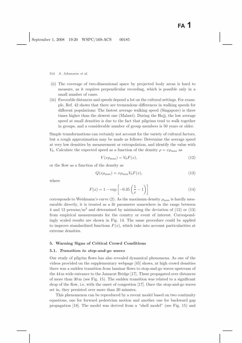
(ii) The coverage of two-dimensional space by projected body areas is hard tomeasure, as it requires perpendicular recording, which is possible only in asmall number of cases.
(iii) Favorable distances and speeds depend a lot on the cultural settings. For exam-ple, Ref. 42 shows that there are tremendous differences in walking speeds fordifferent populations: The fastest average walking speed (Singapore) is threetimes higher than the slowest one (Malawi). During the Hajj, the low averagespeed at small densities is due to the fact that pilgrims tend to walk togetherin groups, and a considerable number of group members is 50 years or older.
Simple transformations can certainly not account for the variety of cultural factors,but a rough approximation may be made as follows: Determine the average speedat very low densities by measurement or extrapolation, and identify the value withV0. Calculate the expected speed as a function of the density ρ = xρmax as
V (xρmax) = V0F (x), (12)
or the flow as a function of the density as
Q(xρmax) = xρmaxV0F (x), (13)
where
F (x) = 1 − exp[−0.35
(1x− 1
)](14)
corresponds to Weidmann’s curve (2). As the maximum density ρmax is hardly mea-surable directly, it is treated as a fit parameter somewhere in the range between4 and 12 persons/m2 and determined by minimizing the deviation of (12) or (13)from empirical measurements for the country or event of interest. Correspond-ingly scaled results are shown in Fig. 14. The same procedure could be appliedto improve standardized functions F (x), which take into account particularities atextreme densities.
5. Warning Signs of Critical Crowd Conditions
5.1. Transition to stop-and-go waves
Our study of pilgrim flows has also revealed dynamical phenomena. As one of thevideos provided on the supplementary webpage [45] shows, at high crowd densitiesthere was a sudden transition from laminar flows to stop-and-go waves upstream ofthe 44m wide entrance to the Jamarat Bridge [17]. These propagated over distancesof more than 30m (see Fig. 15). The sudden transition was related to a significantdrop of the flow, i.e. with the onset of congestion [17]. Once the stop-and-go wavesset in, they persisted over more than 20 minutes.
This phenomenon can be reproduced by a recent model based on two continuityequations, one for forward pedestrian motion and another one for backward gappropagation [18]. The model was derived from a “shell model” (see Fig. 15) and

September 1, 2008 19:20 WSPC/169-ACS 00185
From Crowd Dynamics to Crowd Safety 515
0 0.25 0.5 0.75 10
0.5
1
1.5
Scaled global density
Sca
led
glob
al s
peed
0 0.25 0.5 0.75 10
0.1
0.2
0.3
Scaled density
Sca
led
flow
(a) (b)
Fig. 14. (a) Comparison of scaled empirical measurements of the speed–density relationshipwith Weidmann’s curve (14) (dashed line, see main text for details): The fit parameters for Mori’sand Tsukaguchi’s data [27] (circles) are V0 = 1.40 m/s and ρmax = 9.00 persons/m2, for Poluset al. [32] (squares) they are V0 = 1.25m/s and ρmax = 7.18 persons/m2, for Fruin et al. [5](triangles) they are V0 = 1.30m/s and ρmax = 6.60 persons/m2, for Seyfried et al. [37] (dots)they are V0 = 1.34m/s and ρmax = 5.55 persons/m2, and for our data (thin solid line witherror bars) they are V0 = 0.60m/s and ρmax = 10.79 persons/m2. The rescaling was done byfirst identifying V0, either directly from the data or by extrapolating the speed data towards zerodensity. Then, a least-square fit was performed to find the value of ρmax giving the best match ofEq. (14). Finally, the densities were scaled by ρmax, while the speeds were scaled by V0. It can beseen that scaled speed–density data from different places in the world are reasonably compatible.(b) The compatibility of flow-density data is less obvious, particularly at extreme densities: Thesmooth curve was derived from Weidmann’s speed-density relation (14), while the other solid curvecorresponds to our scaled global flow as a function of the scaled global density. The dashed line(highlighted by circles) represents the scaled local flow (for γ = 0.8) as a function of the scaled localdensity with V0 = 0.86 meters per second and ρmax = 10.57 persons per square meter. Therefore,it must be stressed that flow-density relations should not be derived from speed-density fits, butseparately fitted to empirical flow data.
describes very well the observed alternation between backward gap propagationand forward pedestrian motion.
5.2. Transition to “crowd turbulence”
After the occurence of the stop-and-go waves and the related breakdown of thepedestrian flow, the density reached even higher values and the video recordingsshowed a sudden transition from stop-and-go waves to irregular flows (see Fig. 16).These irregular flows were characterized by random, unintended displacements intoall possible directions, which pushed people around (see Ref. 17 for sample trajec-tories). This “crowd turbulence” caused some individuals to stumble. As the peoplebehind were moved by the crowd as well and could not stop, fallen individuals weretrampled, if they did not get back on their feet quickly enough. Tragically, the areaof trampled people grew more and more in the course of time, as the fallen pilgrimsbecame obstacles for others [17]. The result was one of the biggest crowd disastersin the history of the pilgrimage.
How can we understand this transition to irregular crowd motion? A closer lookat video recordings of the crowd reveals that, at the time when the phenomenon of

September 1, 2008 19:20 WSPC/169-ACS 00185
516 A. Johansson et al.
(a)
(b)
(c) (d)
Fig. 15. (a) Long-term photograph showing stop-and-go waves in a densely packed street. Whilestopped people depicted relatively sharp, people moving from right to left have a fuzzy appearance.Note that gaps propagate from left to right. (b) Empirically observed stop-and-go waves in frontof the entrance to the Jamarat Bridge on January 12, 2006 (after [17]), where pilgrims moved fromleft to right. Light areas correspond to phases of motion, dark colors to stop phases. The “location”coordinate represents the distance to the beginning of the narrowing, i.e. to the cross section ofreduced width. (c) Illustration of the “shell model” (see Ref. 18), in particular of situations whereseveral pedestrians compete for the same gap, which causes coordination problems. (d) Simulationresults of the shell model. The observed stop-and-go waves result from the alternation of forwardpedestrian motion and backward gap propagation.

September 1, 2008 19:20 WSPC/169-ACS 00185
From Crowd Dynamics to Crowd Safety 517
Fig. 16. Long-term photograph of the phenomenon of “crowd turbulence”. In the fuzzy areaof this picture, people are moved into all possible directions by physical forces building up inextremely dense crowds.
“crowd turbulence” occured, people were so densely packed that they were movedinvoluntarily by the crowd. Recently, a computer simulation of this situation wasmade [43]. It managed to reproduce the main observations with an extended socialforce model, assuming that people would try to gain space when the density becomesvery high.
5.3. Measuring critical crowd conditions
For a successful crowd management and control, it is important to know whereand when critical situations are likely to occur, although it must be always kept inmind that not all hazards to the crowd can be reliably detected. Visual inspectionof surveillance cameras is not very suitable to identify critical crowd conditions:While the average density rarely exceeds values of 6 persons per square meter, thelocal densities can vary considerably (see Fig. 11). Moreover, the contour plot ofthe density and its temporal evolution do not give a precise answer, where andwhen the situation becomes critical (see Figs. 17(a) and (b)): At a certain time,the density is high almost everywhere in the recorded area. However, continuousalarms as given by warning systems in the past are not very useful, since securityforces cannot be everywhere. Therefore, it is important to focus their attention andactivity on specific areas.
Also the analysis of the velocity field is not particularly suited to identify criticalareas and times. Figures 17(c) and (d) show the negative divergence of the time-averaged velocity field, which, according to the continuity equation, describes the

September 1, 2008 19:20 WSPC/169-ACS 00185
518 A. Johansson et al.
(a) (b)
(c) (d)
(e) (f)
(g) (h)
Fig. 17. Illustrations of (a, b) the density, (c, d) the negative of the divergence of the velocityfield, (e, f) the curl of the velocity field, and (g, h) the “crowd pressure”. The figures on the leftshow the quantities as functions of space, while the figures on the right show the same quantitiesas functions of time. A color version of these figures can be found on the supplementary web page[45]. The spatial plots are time-averages over the period from 11:45 to 12:30 on January 12, 2006.The arrows show the velocity field, obtained by averaging over the time interval from 11:45 to12:00. Brighter values correspond to higher values. The dashed ellipse indicates the area wherethe crowd accident on January 12, 2006, started.

September 1, 2008 19:20 WSPC/169-ACS 00185
From Crowd Dynamics to Crowd Safety 519
expected relative density increase along the trajectory of a pedestrian.a Moreover,Figs. 17(e) and (f) show the magnitude of the curl of the time-averaged velocityfield measuring the vorticity. Again, these figures give no indication of the time andlocation of the sad crowd accident.
The decisive variable quantifying the hazard to the crowd is rather the varianceof speeds, multiplied by the density. We call this quantity the “(crowd) pressure”.b
It allows one to identify critical locations (see Fig. 17(g)) and times (see Fig. 17(h)).There are even advance warning signs of critical crowd conditions: The crowd acci-dent on January 12, 2006 started about 10 minutes after turbulent crowd motionset in, which happened when the “pressure” exceeded the (R-dependent) value of0.02/s2 [17] (see Fig. 17(h)). Moreover, it occured more than 30 minutes after theaverage flow dropped below the (also R-dependent) threshold of 0.8 pilgrims permeter and second, which can be identified as well by watching out for stop-and-gowaves in accelerated surveillance videos (played fast-forward) [17]. Such advancewarning signs of critical crowd conditions could be evaluated on-line by a videoanalysis system. This would allow one to gain time for corrective measures like flowcontrol, re-routing of people, pressure relief strategies, or the separation of crowdsinto blocks to stop the propagation of shockwaves. Such anticipative crowd controlcould certainly increase the level of safety during future mass events.
6. Summary and Discussion
While most previous measurements of the fundamental diagram for pedestrian flowshave been restricted to densities upto 4 persons/m2, we have measured local densi-ties of 10 persons/m2 and more on the 12th day of the Muslim pilgrimage in 1426Hclose to the entrance ramp of the Jamarat Bridge. The occurrence of such highdensities relates to the body size distribution of pilgrims and implies the possibil-ity of unexpectedly high flow values. Even at densities up to 10 persons/m2, theaverage motion of the crowd is not entirely stopped. This can lead to over-criticalcompressions. However, the density is not the optimum indicator of critical crowdconditions. The “pressure”, defined as the density times the variance of velocities,provides better and more specific information about critical areas and times.
Our results have been obtained with a newly developed, powerful video anal-ysis method for pedestrians, which is well applicable even to dense pedestriancrowds. The automated evaluation delivers pedestrian counts in different direc-tions of motion and measurements of local densities, speeds, flows and pressures.This information can be used for an improved surveillance of the crowd and the
aFrom the continuity equation ∂ρ/∂t+ �∇(ρ�v ) = 0 follows the relative density increase (dρ/dt)/ρ =−�∇�v along the trajectory of a pedestrian, where dρ/dt = ∂ρ/∂t + �v · �∇ρ represents the densitychange in time in the moving system, i.e. along an average trajectory.bThis “gas-kinetic” definition of the pressure is to be distinguished from the mechanical pressureexperienced in a crowd. However, a monotonously increasing functional relationship between bothkinds of pressure is likely, at least when averaging over force fluctuations.
September 1, 2008 19:20 WSPC/169-ACS 00185
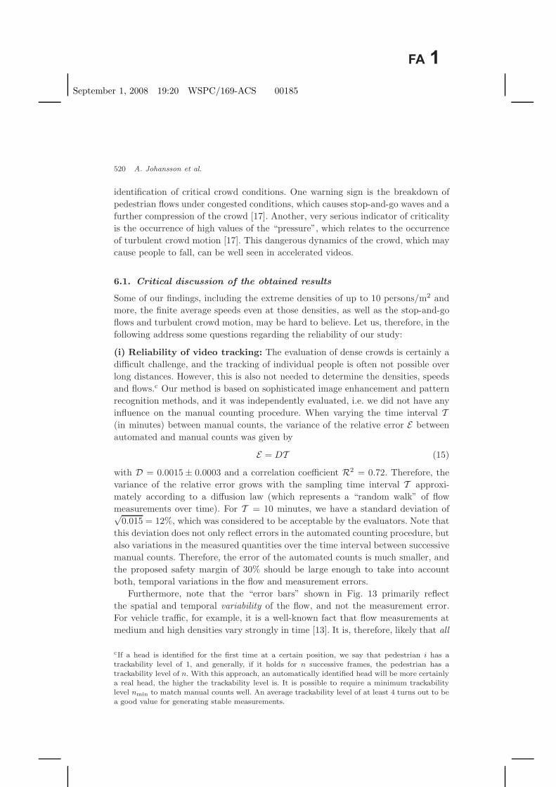
520 A. Johansson et al.
identification of critical crowd conditions. One warning sign is the breakdown ofpedestrian flows under congested conditions, which causes stop-and-go waves and afurther compression of the crowd [17]. Another, very serious indicator of criticalityis the occurrence of high values of the “pressure”, which relates to the occurrenceof turbulent crowd motion [17]. This dangerous dynamics of the crowd, which maycause people to fall, can be well seen in accelerated videos.
6.1. Critical discussion of the obtained results
Some of our findings, including the extreme densities of up to 10 persons/m2 andmore, the finite average speeds even at those densities, as well as the stop-and-goflows and turbulent crowd motion, may be hard to believe. Let us, therefore, in thefollowing address some questions regarding the reliability of our study:
(i) Reliability of video tracking: The evaluation of dense crowds is certainly adifficult challenge, and the tracking of individual people is often not possible overlong distances. However, this is also not needed to determine the densities, speedsand flows.c Our method is based on sophisticated image enhancement and patternrecognition methods, and it was independently evaluated, i.e. we did not have anyinfluence on the manual counting procedure. When varying the time interval T(in minutes) between manual counts, the variance of the relative error E betweenautomated and manual counts was given by
E = DT (15)
with D = 0.0015 ± 0.0003 and a correlation coefficient R2 = 0.72. Therefore, thevariance of the relative error grows with the sampling time interval T approxi-mately according to a diffusion law (which represents a “random walk” of flowmeasurements over time). For T = 10 minutes, we have a standard deviation of√
0.015 = 12%, which was considered to be acceptable by the evaluators. Note thatthis deviation does not only reflect errors in the automated counting procedure, butalso variations in the measured quantities over the time interval between successivemanual counts. Therefore, the error of the automated counts is much smaller, andthe proposed safety margin of 30% should be large enough to take into accountboth, temporal variations in the flow and measurement errors.
Furthermore, note that the “error bars” shown in Fig. 13 primarily reflectthe spatial and temporal variability of the flow, and not the measurement error.For vehicle traffic, for example, it is a well-known fact that flow measurements atmedium and high densities vary strongly in time [13]. It is, therefore, likely that all
cIf a head is identified for the first time at a certain position, we say that pedestrian i has atrackability level of 1, and generally, if it holds for n successive frames, the pedestrian has atrackability level of n. With this approach, an automatically identified head will be more certainlya real head, the higher the trackability level is. It is possible to require a minimum trackabilitylevel nmin to match manual counts well. An average trackability level of at least 4 turns out to bea good value for generating stable measurements.
September 1, 2008 19:20 WSPC/169-ACS 00185
From Crowd Dynamics to Crowd Safety 521
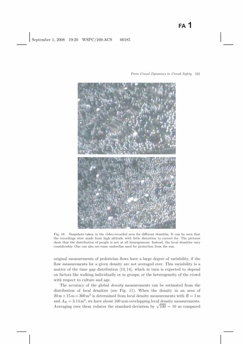
Fig. 18. Snapshots taken in the video-recorded area for different densities. It can be seen thatthe recordings were made from high altitude with little distortion to correct for. The picturesshow that the distribution of people is not at all homogeneous. Instead, the local densities varyconsiderably. One can also see some umbrellas used for protection from the sun.
original measurements of pedestrian flows have a large degree of variability, if theflow measurements for a given density are not averaged over. This variability is amatter of the time gap distribution [13, 14], which in turn is expected to dependon factors like walking individually or in groups, or the heterogeneity of the crowdwith respect to culture and age.
The accuracy of the global density measurements can be estimated from thedistribution of local densities (see Fig. 11). When the density in an area of20m× 15m = 300m2 is determined from local density measurements with R = 1 mand AR = 3.14m2, we have about 100 non-overlapping local density measurements.Averaging over them reduces the standard deviation by
√100 = 10 as compared

September 1, 2008 19:20 WSPC/169-ACS 00185
522 A. Johansson et al.
to the one in Fig. 11, which results in a statistical error of less than 5% for theglobal density. Compared to the variation of the flow, this is negligible, so that itis justified to drop density-related error bars in Figs. 13 and 17, for example.
(ii) Extreme densities: Local densities of up to 10 persons/m2 or slightly morewere not only determined from our video analysis. By evaluation of photographsand independently from us, they were obtained before. Moreover, considerationsbased on projected body areas suggest that densities upto 11 persons/m2 wouldbe possible in principle [38], which is consistent with our results. Furthermore,Mori’s and Tsukaguchi’s data [27] come close to our measurements, when the scalinganalysis of Fig. 14 is applied. The importance of the body size distribution can alsobe seen in Refs. [30, 31, 39].
(iii) Flow-density relationship: More important than the maximum possibledensity (which should be avoided anyway) are the maximum global flow (as itdetermines the capacity of a pedestrian facility) and the density at which the flowstarts to drop (which gives rise to congestion and a further increase of the density).It should be stressed that an occurence of the maximum flow should be avoided fortwo reasons: first, in order to prevent a breakdown of the flow and second, becausethe density at which the maximum flow is reached is not comfortable to pedestriansanymore [5].
Note that both, our local and global flow–density relations look different fromthe fundamental diagrams reported in the literature. In order to check the plausi-bility of our findings, we have scaled our data by the maximum density ρmax (whichdepends on the projected body area) and by the average desired velocity V0 (whichis smaller for pilgrims than usual as they often walk in large groups including peopleaged 50 years and older). Our scaled speed–density data shown in Fig. 14(a) agreewell with other measurements, which indicates their compatibility, while we finddeviations for the flow-density data at spatial occupancies of 0.6 and higher (seeFig. 14(b)). These deviations can have different origins: In some cases, fundamen-tal diagrams have been determined by fitting speed–density data and multiplyingthem with the density. The resulting fit curve will not necessarily represent flow–density data well, as the flow–density relationship is sensitive to deviations in thespeed–density relationship. Furthermore, the data for the Hajj are expected to dif-fer from measurements for other situations in which dense crowds do not move(e.g. on the platform of a subway station or in front of a stage). Therefore, thequestion is whether the main distinguishing feature, the second increase in the flowat extreme densities, is an artifact of our evaluation method or represents a realfact.
(iv) Second increase in the flow at extreme densities: This increase resultsfrom the measurement of finite average speeds even at extreme densities. In fact,it can be observed in the evaluated video recordings that (apart from intermediatestops reflecting stop-and-go motion) people kept moving at all observed densities,

September 1, 2008 19:20 WSPC/169-ACS 00185
From Crowd Dynamics to Crowd Safety 523
even after the accident occured and some areas were difficult to pass. People try toget out of areas of extreme density — this is why the average speed stays finite.
It should be noted that the second increase of the flow has important implica-tions for the dynamics [2]. In particular, it implies the coexistence of forward andbackward moving shock waves. The minimum of the flow–density curve at finitedensities and crowd turbulence are two closely related properties. And as crowdturbulence is well visible in the video recordings, when played in fast-forward mode(see the videos at http://www.trafficforum.org/crowdturbulence), a second increasein the density is actually expected to exist.
(v) Stop-and-go motion and crowd turbulence: Both phenomena have notonly been observed once and in a single location. Stop-and-go waves can occur inlarge spatial areas and persist over many minutes, and we have seen the phenomenain recordings of different locations. The same applies to crowd turbulence. It hasnot only occured in January 2006, but also in previous years, and the observation isconsistent with what Fruin has reported [6]: “At occupancies of about 7 persons/m2
the crowd becomes almost a fluid mass. Shock waves can be propagated through themass, sufficient to . . . propel them distances of 3m or more. . . . Access to those whofall is impossible.” This visualizes the conditions in extremely dense crowds quitewell, and it is compatible with the location of the minimum in our flow–densitydata.
(vi) Local global dependencies: It is clear that locally measured quantities varymore than global ones. If one averages over many local measurements, the maximumdensity and speed or flow are, of course, reduced. Nevertheless, according to Fig.14(b), the local and global curves agree surprisingly well, when the densities andspeeds are scaled by the respective maximum values V0 and ρmax. As the local andglobal quantities have been determined in different ways, this is a good reason totrust the corresponding data.
(vii) Alarms of critical crowd conditions: The Hajj is in many ways an extremeevent, with potentially critical situations occuring at different locations. If alarmsare given whenever the global density exceeds a certain density defined to be crit-ical, it is difficult to take specific actions. Such alarms may continue over manyhours. The pressure-based method, in contrast, would give a warning of potentiallyturbulent crowd motion over a short time period, and would indicate critical loca-tions. It is no problem if the critical pressure (here: 0.02/s2) is shortly crossed beforecrowd turbulence takes over in a large area. This gives security forces a bit moretime to prepare counter actions.
Note, however, that counter actions should be taken much earlier, at latestwhen stop-and-go waves set in, as this indicates a breakdown of the flow. It shouldalso be underlined that the critical flow of 0.8m/s [17] and the critical pressureof 0.02/s2 depend on the parameters of the measurement method, in particularthe choice of R, and it may depend on other factors like the kind of crowd aswell. As a consequence, these critical thresholds need to be properly calibrated.

September 1, 2008 19:20 WSPC/169-ACS 00185
524 A. Johansson et al.
In fact, rather than an automated alarm system we propose to view acceleratedvideo sequences, which allows one to easily discover areas where a smooth flow isdisturbed, where stop-and-go waves appear or where even crowd turbulence occurs.Furthermore, it would be helpful to enhance surveillance videos by overlayingadditional information like the intensity of the crowd pressure, as illustrated bythe video at http://www.trafficforum.org/crowdturbulence/pressure video.mpg
6.2. Some measures to improve crowd safety
In the interest of crowd safety, densities higher than 3–4 persons/m2 in largecrowds and particularly the onset of stop-and-go waves or crowd turbulence mustbe avoided. Therefore, a combination of the following measures is recommended:
(i) Design: The infrastructure should be designed in a way that no bottlenecksor objects (e.g. luggage) will obstruct the flow. This can be quite challenging,if the usage patterns are changing. In particular, it must be avoided that theoutflow capacity is smaller than the inflow capacity. Accumulations of largecrowds should be avoided. If this is impossible, the outflow capacities must bedimensioned such that the time to evacuate the area is much shorter than thetime to fill it. (It should not exceed a few minutes.) Furthermore, a system ofemergency routes or, more generally, a “valve system” is required to be ableto reduce pressures in certain areas of the system, where needed.
(ii) Operation: The infrastructure should be operated in a way that avoids coun-terflows or intersecting flows. Even merging flows may cause serious problems.Flows of people should be re-balanced if there is a large utilization in certainparts of the system while there is still available capacity in others. Obstacles(including people blocking the ways) should be removed from areas intendedfor moving. Some ways should be reserved for emergency operation and pro-tected from public access.
(iii) Monitoring: Areas of accumulation or any possible conflict points (includingcrossing flows or bottlenecks, if these are really unavoidable in the system)must be monitored during highly frequented time periods. To support thejob of the monitoring crew and guide security forces to the right places, it ishelpful to display additional information in the surveillance videos, visualizing,for example, the density, the flow, and/or the crowd pressure.
(iv) Crowd Management: In certain events, the flow must be suitably limited tothe safe capacity of the system (which should consider a safety margin of30%). This may be done by applying a scheduling program, which is a planregulating the timing and routing of groups of people. The compliance with thescheduling program must be carefully monitored (e.g. by control points and/orGPS tracking), and deviations from it must be counter-acted (e.g. by fines).Moreover, an adaptive re-scheduling should be possible in order to respondproperly to the actual conditions in the system. It is even more favorable to

September 1, 2008 19:20 WSPC/169-ACS 00185
From Crowd Dynamics to Crowd Safety 525
have a simulation tool for the prediction of the flows in the system. This wouldallow an anticipative crowd management.
(v) Contingency Plans: For situations, where the system enters a critical statefor whatever reason (e.g a fire, an accident, violent behavior, or bad weatherconditions), one needs to have detailed contingency plans, which must beworked out and exercised in advance.
The above is a list of only some of the measures that can be taken to improve crowdsafety. For further measures see Refs. [7, 9–11,22, 29, 38, 40].
Acknowledgments
The authors are grateful for the partial financial support by the DFG grant He2789/7-1 and the ETH Research Grant CH1-01 08-2. They would like to thank theSTESA staff for converting the large number of video recordings, and the MoMRAstaff for doing the manual counting. Furthermore, the authors appreciate fruitfuldiscussions with Martin Treiber, who proposed the local density measure, and withKarl Walkow, who collected and digitized empirical pedestrian data from othersources for comparison with our measurements.
References
[1] Burstedde, C., Klauck, K., Schadschneider, A. and Zittartz, J., Simulation of pedes-trian dynamics using a two-dimensional cellular automaton, Physica A 295 (2001)507–525.
[2] Colombo, R. M. and Rosini, M. D., Pedestrian flows and non-classical shocks, Math.Methods Appl. Sci. 28 (2005) 1553–1567.
[3] Dussutour, A., Fourcassie, V., Helbing, D. and Deneubourg, J.-L., Optimal trafficorganization in ants under crowded conditions, Nature 428 (2004) 70–73.
[4] Epstein, J. and Axtell, R., Growing Artificial Societies. Social Science from the Bot-tom Up (Brookings Institution/MIT Press, Washington, DC, 1996).
[5] Fruin, J. J., Designing for pedestrians: A level-of-service concept, Highway Res. Rec.355 (1971) 1–15.
[6] J. J. Fruin, The causes and prevention of crowd disasters, in Engineering for CrowdSafety, R. A. Smith and J. F. Dickie (eds.) (Elsevier, Amsterdam, 1993), pp. 99–108.
[7] Government of Canada, Emergency preparedness guidelines for mass, crowd-intensive events, see http://ww3.psepc-sppcc.gc.ca/research/resactivites/planPrep/en crowd/1993-D011 e.pdf (1994).
[8] Haken, H., Synergetics — An Introduction (Springer, Berlin, 1983).[9] Health and Safety Executive, Steps to Risk Assessment — Case Studies (HSE Books,
Norwich, 1998).[10] Health and Safety Executive, The Event Safety Guide (HSE Books, Norwich, 1999).[11] Health and Safety Executive, Managing Crowds Safely (HSE Books, Norwich, 2000).[12] Helbing, D., Quantitative Sociodynamics. Stochastic Methods and Models of Social
Interaction Processes (Kluwer Academic, Dordrecht, 1995).[13] Helbing, D., Traffic and related self-driven many-particle systems. Rev. Mod. Phys.
73 (2001) 1067–1141.

September 1, 2008 19:20 WSPC/169-ACS 00185
526 A. Johansson et al.
[14] Helbing, D., Buzna, L., Johansson, A. and Werner, T., Self-organized pedestriancrowd dynamics: Experiments, simulations, and design solutions, Transport. Sci. 39(2005) 1–24.
[15] Helbing, D., Farkas, I., Molnar, P. and Vicsek, T., Simulation of pedestriancrowds in normal and evacuation situations, in Pedestrian and EvacuationDynamics, M. Schreckenberg and S. D. Sharma (eds.) (Springer-Verlag, Heidelberg,2002), pp. 21–58.
[16] Helbing, D., Farkas, I. and Vicsek, T., Simulating dynamical features of escape panic,Nature 407 (2000) 487–490.
[17] Helbing, D., Johansson, A. and Al-Abideen, H. Z., The dynamics of crowd disasters:An empirical study, Phys. Rev. E 75 (2007) 046109.
[18] Helbing, D., Johansson, A., Mathiesen, J., Jensen, M. H. and Hansen, A., Analyticalapproach to continuous and intermittent bottleneck flows, Phys. Rev. Lett. 97 (2006)168001.
[19] Helbing, D. and Molnar, P., Social force model for pedestrian dynamics, Phys. Rev.E 51 (1995) 4282–4286.
[20] Hoogendoorn, S. P. and Daamen, W., Pedestrian behavior at bottlenecks, Transport.Sci. 39 (2005) 147–159.
[21] Hoogendoorn, S. P., Daamen, W. and Bovy, P. H. L., Extracting microscopic pedes-trian characteristics from video data, 82nd Transportation Research Board AnnualMeeting (CD-ROM, Washington DC: National Academy Press, 2003).
[22] Independent Street Arts Network, Safety Guidance for Street Arts, Carnival, Pro-cessions, and Large-Scale Performances (Independent Street Arts Network, London,2004).
[23] Isobe, M., Helbing, D. and Nagatani, T., Experiment, theory and simulation of theevacuation of a room without visibility. Phys. Rev. E 69 (2004) 066132.
[24] Johansson, A., Data-driven modeling of pedestrian crowds, Ph.D. thesis, in prepara-tion, Dresden University of Technology, Dresden (2008).
[25] Kerridge, J., Keller, S., Chamberlain, T. and Sumpter, N., Collecting pedestrian tra-jectory data in real-time, in Pedestrian and Evacuation Dynamics 2005, N. Waldauet al. (eds.), 27–39 (Springer-Verlag, Heidelberg, 2007).
[26] Kretz, T., Grunebohm, A. and Schreckenberg, M., Experimental study of pedestrianflow through a bottleneck, J. Stat. Mech. (2006), p. 10014.
[27] Mori, M. and Tsukaguchi, H., A new method for evaluation of level of service inpedestrian facilities, Transport. Res. A 21 (1987) 223–234 .
[28] Moussaid, M., Garnier, S., Helbing, D., Johansson, A. and Theraulaz, G., Extractinglaws of human interaction from pedestrian experiments, Submitted.
[29] Musterversammlungsstattenverordnung 2005, see http://www.versammlungsstaett-enverordnung.de/vstaettv neu/bundeslaender/downloads/MusterVstaettV2005/MVStaettV 2005.pdf (2005).
[30] Pauls, J. L., Fruin, J. J. and Zupan, J. M., Minimum stair-width for evacuation,overtaking movement and counterflow — Technical bases and suggestions for thepast, present and future, in Pedestrian and Evacuation Dynamics 2005, N. Waldauet al. (eds.) (Springer-Verlag, Heidelberg, 2007), pp. 57–69.
[31] Pheasant, S. T., Bodyspace: Anthropometry, Ergonomics, and the Design of Work(Taylor and Francis, London, 1998).
[32] Polus, A., Schofer, J. L. and Ushpiz, A., Pedestrian flow and level of service, J.Transport. Eng. 109 (1983) 46–56.
[33] Predtechenskii, V. M. and Milinskii, A. I., Planning for Foot Traffic Flow in Buildings(Amerind, New Delhi, 1978).

September 1, 2008 19:20 WSPC/169-ACS 00185
From Crowd Dynamics to Crowd Safety 527
[34] Saloma, C., Perez, G. J., Tapang, G., Lim, M. and Palmes-Saloma, C., Self-organizedqueuing and scale-free behavior in real escape panic, PNAS 100 (2003) 11947–11952.
[35] Schadschneider, A., Klingsch, W., Kluepfel, H., Kretz, T., Rogsch, C. and Seyfried, A.Evacuation dynamics: Empirical results, modeling and applications, arXiv:0802.1620(2008).
[36] Schweitzer, F., Brownian Agents and Active Particles. Collective Dynamics in theNatural and Social Sciences (Springer, Berlin, 2003).
[37] Seyfried, A., Steffen, B., Klingsch, W. and Boltes, M., The fundamental diagram ofpedestrian movement revisited, J. Stat. Mech. (2005), p. 10002.
[38] Still, K., Crowd Dynamics, Ph.D. thesis, University of Warwick, Warwick (2000).[39] Teknomo, K., Microscopic pedestrian flow characteristics: Development of an image
processing data collection and simulation model, Ph.D. thesis, Tohoku UniversityJapan, Sendai (2002).
[40] The Scottish Office, Guide to Safety at Sports Grounds (The Stationery Office, Nor-wich, 4th edition, 1997).
[41] Weidmann, U., Transporttechnik der Fußganger (Schriftenreihe des Institut furVerkehrsplanung, Transporttechnik, Straßen- und Eisenbahnbau 90, ETH Zurich,Zurich, 1993).
[42] Wiseman, R. Pace of Life, http://www.paceoflife.co.uk/ (2008).[43] Yu, W. and Johansson, A., Modeling crowd turbulence by many-particle simulations,
Phys. Rev. E 76 (2007) 046105.[44] Richtlinie fur Mikroskopische Entfluchtungsanalysen (in German) The RiMEA
Project http://www.rimea.de/downloads.html (2008).[45] Supplementary web page, http://www.trafficforum.org/crowdturbulence (2007).

September 1, 2008 19:20 WSPC/169-ACS 00185