From Basic Concepts to Actual Calculations

P1: GKW/UKS P2: GKW/UKS QC: GKW

CB228/Cercignani CB228-FM October 27, 1999 15:52 Char Count= 44423

Rarefied Gas DynamicsFrom Basic Concepts to Actual Calculations

CARLO CERCIGNANIDepartment of Mathematics

Politechnic University of Milan

v



P U B L I S H E D B Y T H E P R E S S S Y N D I C A T E O F T H E U N I V E R S I T Y O F C A M B R I D G E

The Pitt Building, Trumpington Street, Cambridge, United Kingdom

C A M B R I D G E U N I V E R S I T Y P R E S S

The Edinburgh Building, Cambridge CB2 2RU, UK http://www.cup.cam.ac.uk40 West 20th Street, New York, NY 10011-4211, USA http://www.cup.org

10 Stamford Road, Oakleigh, Melbourne 3166, AustraliaRuiz de Alarcon 13, 28014 Madrid, Spain

c© Cambridge University Press 2000

This book is in copyright. Subject to statutory exceptionand to the provisions of relevant collective licensing agreements,

no reproduction of any part may take place withoutthe written permission of Cambridge University Press.

First published 2000

Printed in the United States of America

TypefaceTimes Roman 10/13 pt. SystemLATEX 2ε [TB]

A catalog record for this book is available fromthe British Library.

Library of Congress Cataloging in Publication Data

Cercignani, Carlo.

Rarefied gas dynamics : from basic concepts to actual calculations/ Carlo Cercignani.

p. cm. – (Cambridge texts in applied mathematics)

Includes bibliographical references.

ISBN 0-521-65008-9 (hardback). – ISBN 0-521-65992-2 (pbk.)

1. Gas dynamics. I. Title. II. Series.

QA930.C34 2000

533′.2 – dc21 99-15475CIP

vi



Contents

Preface page xi

Introduction xiii

1 Boltzmann Equation and Gas–Surface Interaction 11.1 Introduction 11.2 The Boltzmann Equation 21.3 Molecules Different from Hard Spheres 91.4 Collision Invariants 111.5 The Boltzmann Inequality and the Maxwell Distributions 151.6 The Macroscopic Balance Equations 161.7 TheH -Theorem 211.8 Equilibrium States and Maxwellian Distributions 241.9 Model Equations 261.10 The Linearized Collision Operator 291.11 Boundary Conditions 30

References 38

2 Problems for a Gas in a Slab: General Aspectsand Preliminary Example 40

2.1 Introduction 402.2 Couette Flow for Bounce-Back Boundary Conditions 432.3 Couette Flow at Small Mean Free Paths 502.4 Couette Flow at Large Mean Free Paths 582.5 Rarefaction Regimes 642.6 Moment Methods for Plane Couette Flow 672.7 Perturbations of Equilibria 75

References 80

vii



viii Contents

3 Problems for a Gas in a Slab or a Half-Space: Discussionof Some Solutions 82

3.1 Use of Models 823.2 Transformation of Models into Pure Integral Equations 853.3 Variational Methods 873.4 Poiseuille Flow 983.5 Half-Space Problems 1033.6 Numerical Methods 1133.7 The Direct Simulation Monte Carlo Method 1173.8 A Test Case: Couette Flow with Reverse Reflection 1193.9 Accurate Numerical Solutions of the Linearized

Boltzmann Equation 122References 124

4 Propagation Phenomena and Shock Waves in Rarefied Gases 1294.1 Introduction 1294.2 Propagation of Discontinuities 1304.3 Shear, Thermal, and Sound Waves 1354.4 Shock Waves 1414.5 Monte Carlo Simulation and the Problem of Shock Wave

Structure 1524.6 Concluding Remarks 156

References 157

5 Perturbation Methods in More than One Dimension 1625.1 Introduction 1625.2 Linearized Steady Problems 1625.3 Linearized Solutions of Internal Problems 1685.4 Linearized Solutions of External Problems 1705.5 The Stokes Paradox in Kinetic Theory 1735.6 The Continuum Limit 1805.7 Free Molecular Flows 1895.8 Nearly Free Molecular Flows 1925.9 Expansion of a Gas into a Vacuum 1945.10 Concluding Remarks 199

References 200

6 Polyatomic Gases, Mixtures, Chemistry, and Radiation 2046.1 Introduction 2046.2 Mixtures 205



Contents ix

6.3 Polyatomic Gases 2096.4 TheH -Theorem for Classical Polyatomic Molecules 2166.5 Chemical Reactions 2206.6 Ionization and Thermal Radiation 2256.7 Concluding Remarks 226

References 227

7 Solving the Boltzmann Equation by Numerical Techniques 2307.1 Introduction 2307.2 The DSMC Method 2317.3 Applications of the DSMC Method to Rarefied Flows 2347.4 Vortices and Turbulence in a Rarefied Gas 2417.5 Qualitative Differences between the Navier–Stokes and

the Boltzmann Models 2527.6 Discrete Velocity Models 2567.7 Concluding Remarks 263

References 266

8 Evaporation and Condensation Phenomena 2738.1 Introduction 2738.2 The Knudsen Layer near an Evaporating Surface 2778.3 The Knudsen Layer near a Condensing Surface 2858.4 Influence of the Evaporation–Condensation Coefficient 2908.5 Moderate Rates of Evaporation and Condensation 2938.6 Effects due to the Presence of a Noncondensable Gas

and to the Internal Degrees of Freedom 2998.7 Evaporation from a Finite Area 3048.8 Concluding Remarks 306

References 307

Index 313

P1: FKF/LQA P2: FKF

CB228/Cercignani CB228-01 September 22, 1999 5:48 Char Count= 116856

1Boltzmann Equation and Gas–Surface Interaction

1.1. Introduction

According to kinetic theory, a gas in normal conditions (no chemical reactions,no ionization phenomena, etc.) is formed of elastic molecules rushing hitherand thither at high speed, colliding and rebounding according to the laws ofelementary mechanics. In this and the next section, the molecules of a gaswill be assumed to be hard, elastic, and perfectly smooth spheres. Later weshall consider molecules as centers of forces that move according to the lawsof classical mechanics and, starting with Chapter 6, more complex modelsdescribing polyatomic molecules.

The rules generating the dynamics of many spheres are easy to describe:Thus, for example, if no external forces, such as gravity, are assumed to acton the molecules, each of them will move in a straight line unless it happensto strike another molecule or a solid wall. The phenomena associated with thisdynamics are not so simple, especially when the number of spheres is large.It turns out that this complication is always present when dealing with a gas,because the number of molecules usually considered is extremely large: Thereare about 2.7 · 1019 in a cubic centimeter of a gas at atmospheric pressure anda temperature of 0◦C.

Given the vast number of particles to be considered, it would of course bea hopeless task to attempt to describe the state of the gas by specifying theso-called microscopic state (i.e., the position and velocity of every individ-ual sphere); we must have recourse to statistics. A description of this kind ismade possible because in practice all that our typical observations can detectare changes in the macroscopic state of the gas, described by quantities suchas density, bulk velocity, temperature, stresses, and heat flow, and these arerelated to some suitable averages of quantities depending on the microscopicstate.

1

P1: FKF/LQA P2: FKF


2 1 Boltzmann Equation and Gas–Surface Interaction

1.2. The Boltzmann Equation

The exact dynamics ofN particles is a useful conceptual tool, but it cannot inany way be used in practical calculations because it requires a huge numberof real variables (of the order of 1020). This was realized by Maxwell andBoltzmann when they started to work with the one-particle probability density,or distribution functionP(1)(x, ξ, t). The latter is a function of seven variables:the components of the two vectorsx andξ and timet . In particular, Boltzmannwrote an evolution equation forP(1) by means of a heuristic argument, whichwe shall try to present in such a way as to show where extra assumptions areintroduced.

Let us first consider the meaning ofP(1)(x, ξ, t); it gives the probabilitydensity of finding one fixed particle (say, the one labeled by 1) at a certain point(x, ξ) of the six-dimensional reduced phase space associated with the positionand velocity of that molecule. To simplify the treatment, we shall for the momentassume that the molecules are hard spheres, whose center has positionx. Whenthe molecules collide, momentum and kinetic energy must be conserved; thus(Problem 1.2.2) the velocities after the impact,ξ′1 andξ′2, are related to thosebefore the impact,ξ1 andξ2, by

ξ′1 = ξ1− n[n · (ξ1− ξ2)],

ξ′2 = ξ2+ n[n · (ξ1− ξ2)], (1.2.1)

wheren is the unit vector alongξ1− ξ′1. Note that the relative velocity

V = ξ1− ξ2 (1.2.2)

satisfies

V′ = V − 2n(n · V), (1.2.3)

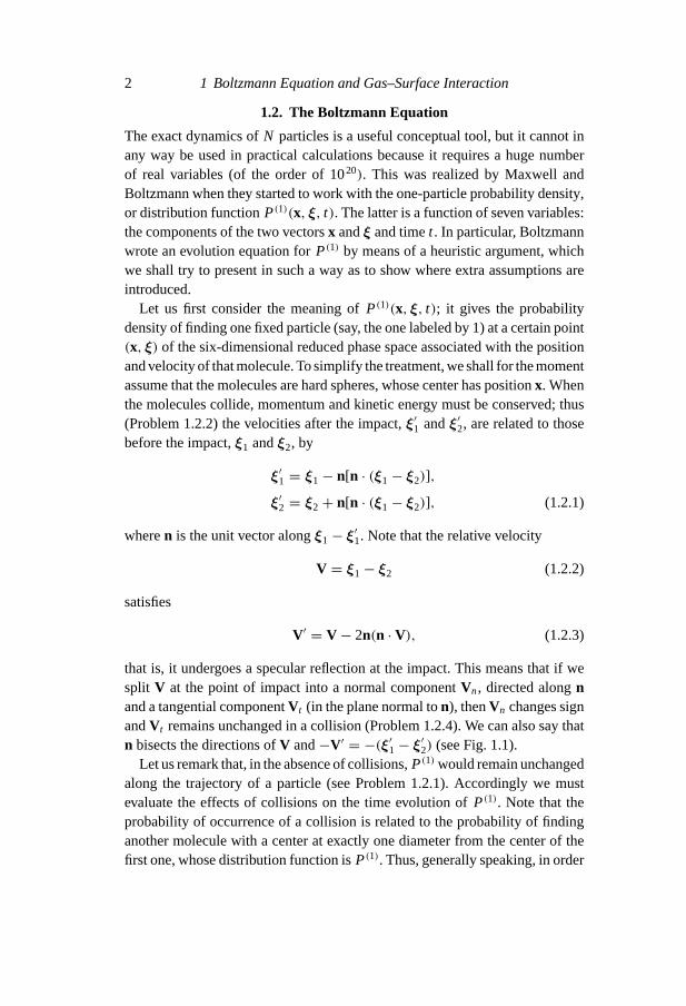
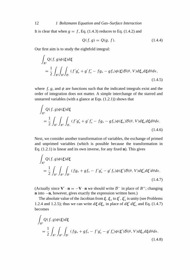
that is, it undergoes a specular reflection at the impact. This means that if wesplit V at the point of impact into a normal componentVn, directed alongnand a tangential componentVt (in the plane normal ton), thenVn changes signandVt remains unchanged in a collision (Problem 1.2.4). We can also say thatn bisects the directions ofV and−V′ = −(ξ′1− ξ′2) (see Fig. 1.1).

Let us remark that, in the absence of collisions,P(1) would remain unchangedalong the trajectory of a particle (see Problem 1.2.1). Accordingly we mustevaluate the effects of collisions on the time evolution ofP(1). Note that theprobability of occurrence of a collision is related to the probability of findinganother molecule with a center at exactly one diameter from the center of thefirst one, whose distribution function isP(1). Thus, generally speaking, in order

P1: FKF/LQA P2: FKF


1.2 The Boltzmann Equation 3

Figure 1.1. The directions of the relative velocities before and after the impact arebisected by the unit vectorn.

to write the evolution equation forP(1) we shall need another function,P(2),that gives the probability density of finding, at timet , the first molecule atx1 with velocity ξ1 and the second atx2 with velocity ξ2; obviously P(2) =P(2)(x1, x2, ξ1, ξ2, t). HenceP(1) satisfies an equation of the following form:

∂P(1)

∂t+ ξ1 ·

∂P(1)

∂x1=G− L . (1.2.4)

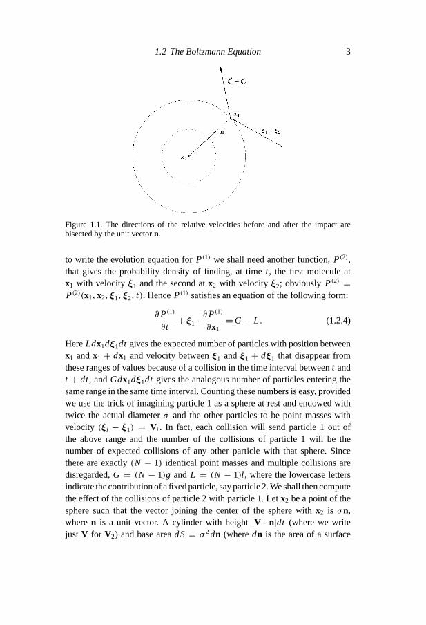
HereLdx1dξ1dt gives the expected number of particles with position betweenx1 andx1 + dx1 and velocity betweenξ1 andξ1 + dξ1 that disappear fromthese ranges of values because of a collision in the time interval betweent andt + dt, andGdx1dξ1dt gives the analogous number of particles entering thesame range in the same time interval. Counting these numbers is easy, providedwe use the trick of imagining particle 1 as a sphere at rest and endowed withtwice the actual diameterσ and the other particles to be point masses withvelocity (ξi − ξ1) = V i . In fact, each collision will send particle 1 out ofthe above range and the number of the collisions of particle 1 will be thenumber of expected collisions of any other particle with that sphere. Sincethere are exactly(N − 1) identical point masses and multiple collisions aredisregarded,G = (N − 1)g and L = (N − 1)l , where the lowercase lettersindicate the contribution of a fixed particle, say particle 2. We shall then computethe effect of the collisions of particle 2 with particle 1. Letx2 be a point of thesphere such that the vector joining the center of the sphere withx2 is σn,wheren is a unit vector. A cylinder with height|V · n|dt (where we writejust V for V2) and base areadS= σ 2dn (wheredn is the area of a surface

P1: FKF/LQA P2: FKF



Figure 1.2. Calculation of the number of collisions between two molecules.

element of the unit sphere aboutn) will contain the particles with velocityξ2

hitting the basedSin the time interval(t, t + dt) (see Fig. 1.2); its volume isσ 2dn|V ·n|dt. Thus the number of collisions of particle 2 with particle 1 in theranges(x1, x1+ dx1), (ξ1, ξ1+ dξ1), (x2, x2+ dx2), (ξ2, ξ2+ dξ2), (t, t+ dt)occuring at points ofdSis P(2)(x1, x2, ξ1, ξ2, t) dx1dξ1dξ2σ

2dn|V2 · n|dt. Ifwe want the number of collisions of particle 1 with 2, when the range of theformer is fixed but the latter may have any velocityξ2 and any positionx2 on thesphere (i.e., anyn), we integrate over the sphere and all the possible velocitiesof particle 2 to obtain

ldx1dξ1dt= dx1dξ1dt∫

R3

∫B−

P(2)(x1, x1+ σn, ξ1, ξ2, t)|V · n|σ 2dndξ2,

(1.2.5)

whereB− is the hemisphere corresponding toV · n< 0 (the particles are movingtoward each other before the collision). Thus we have the following result:

L = (N − 1)σ 2∫

R3

∫B−

P(2)(x1, x1+ σn, ξ1, ξ2, t)|(ξ2− ξ1) · n|dξ2dn.

(1.2.6)

The calculation of the gain termG is exactly the same as the one forL, except forthe fact that we have to integrate over the hemisphereB+, defined byV ·n > 0(the particles are moving away from each other after the collision). Thus we have

G = (N − 1)σ 2∫

R3

∫B+

P(2)(x1, x1+ σn, ξ1, ξ2, t)|(ξ2− ξ1) · n|dξ2dn.

(1.2.7)

We thus could write the right-hand side of Eq. (1.2.4) as a single expression:

G− L = (N − 1)σ 2∫

R3

∫B

P(2)(x1, x1+ σn, ξ1, ξ2, t)(ξ2− ξ1) · ndξ2dn,

(1.2.8)

P1: FKF/LQA P2: FKF



where nowB is the entire unit sphere and we have abolished the bars of absolutevalue in the right-hand side.

Equation (1.2.8), although absolutely correct, is not so useful. It turns out tobe much more convenient to keep the gain and loss terms separated. Only inthis way, in fact, can we insert in Eq. (1.2.4) the information that the probabilitydensityP(2) is continuous at a collision; in other words, although the velocitiesof the particles undergo the discontinuous change described by Eqs. (1.2.1), wecan write

P(2)(x1, ξ1, x2, ξ2, t) = P(2)(x1, ξ1− n(n · V), x2, ξ2+ n(n · V), t)if |x1− x2| = σ. (1.2.9)

For brevity, we write (in agreement with Eq. (1.2.1)

ξ′1 = ξ1− n(n · V), ξ′2 = ξ2+ n(n · V). (1.2.10)

Inserting Eq. (1.2.8) in Eq. (1.2.5) we thus obtain

G = (N − 1)σ 2∫

R3

∫B+

P(2)(x1, x1+ σn, ξ′1, ξ′2, t)|(ξ2− ξ1) · n|dξ2dn,

(1.2.11)

which is a frequently used form. Sometimesn is changed into−n to have thesame integration range as inL; the only change (in addition to the change inthe range) is in the second argument ofP(2), which becomesx1− σn.

At this point we are ready to understand Boltzmann’s argument.N is a verylarge number andσ (expressed in common units, such as, e.g., centimeters)is very small; to fix the ideas, let us consider a box whose volume is 1 cm3 atroom temperature and atmospheric pressure. ThenN ∼= 1020 andσ ∼= 10−8 cm.Then(N−1)σ 2 ∼= Nσ 2 ∼= 104 cm2 = 1 m2 is a sizable quantity, while we canneglect the difference betweenx1 andx1+ σn. This means that the equation tobe written can be rigorously valid only in the so-calledBoltzmann–Grad limit,whenN →∞, σ → 0 with Nσ 2 finite.

In addition, the collisions between two preselected particles are rather rareevents. Thus two spheres that happen to collide can be thought to be two ran-domly chosen particles and it makes sense to assume that the probability densityof finding the first molecule atx1 with velocityξ1 and the second atx2 with ve-locity ξ2 is the product of the probability density of finding the first molecule atx1 with velocityξ1 times the probability density of finding the second moleculeatx2 with velocityξ2. If we accept this we can write (assumption ofmolecularchaos)

P(2)(x1, ξ1, x2, ξ2, t) = P(1)(x1, ξ1, t)P(1)(x2, ξ2, t) (1.2.12)

P1: FKF/LQA P2: FKF



for two particles that are about to collide, or

P(2)(x1, ξ1, x1+ σn, ξ2, t) = P(1)(x1, ξ1, t)P(1)(x1, ξ2, t)

for (ξ2− ξ1) · n < 0. (1.2.13)

Thus we can apply this recipe to the loss term (1.2.4) but not to the gain termin the form (1.2.5). It is possible, however, to apply Eq. (1.2.13) (withξ′1, ξ

′2 in

place ofξ1, ξ2) to the form (1.2.9) of the gain term, because the transformation(1.2.10) maps the hemisphereB+ onto the hemisphereB−.

If we accept all the simplifying assumptions made by Boltzmann, we obtainthe following form for the gain and loss terms:

G= Nσ 2∫

R3

∫B−

P(1)(x1, ξ′1, t)P

(1)(x1, ξ′2, t)|(ξ2− ξ1) · n|dξ2dn, (1.2.14)

L = Nσ 2∫

R3

∫B−

P(1)(x1, ξ1, t)P(1)(x1, ξ2, t)|(ξ2− ξ1) · n|dξ2dn. (1.2.15)

By inserting these expressions in Eq. (1.2.6) we can write theBoltzmann equa-tion in the following form:

∂P(1)

∂t+ ξ1 ·

∂P(1)

∂x1= Nσ 2

∫R3

∫B−

[P(1)(x1, ξ

′1, t)P

(1)(x1, ξ′2, t)

− P(1)(x1, ξ1, t)P(1)(x1, ξ2, t)

] |(ξ2− ξ1) · n|dξ2dn. (1.2.16)

We remark that the expressions forξ′1 andξ′2 given in Eq. (1.2.1) are by nomeans the only possible ones. In fact we might use a different unit vectorω,directed asV′, instead ofn. Then Eq. (1.2.1) is replaced by

ξ′1 = ξ +1

2|ξ1− ξ2|ω,

ξ′2 = ξ −1

2|ξ1− ξ2|ω, (1.2.17)

whereξ = 12(ξ1+ξ2) is the velocity of the center of mass. The relative velocity

V satisfies

V′ = ω|V|. (1.2.18)

The Boltzmann equation is an evolution equation forP(1), without any referenceto P(2). This is its main advantage. However, it has been obtained at the price of

P1: FKF/LQA P2: FKF



several assumptions; the chaos assumption present in Eqs. (1.2.12) and (1.2.13)is particularly strong and requires discussion.

The molecular chaos assumption is clearly a property of randomness. In-tuitively, one feels that collisions exert a randomizing influence, but it wouldbe completely wrong to argue that the statistical independence described byEq. (1.2.12) is a consequence of the dynamics. It is quite clear that we cannotexpect every choice of the initial distribution of positions and velocities of themolecules to give aP(1) that agrees with the solution of the Boltzmann equationin the Boltzmann–Grad limit. In other words molecular chaos must be presentinitially and we can only ask whether it is preserved by the time evolution ofthe system of hard spheres.

It is evident that the chaos property (1.2.12), if initially present, is almostimmediately destroyed, if we insist that it should be valid everywhere. In fact,if it were strictly valid everywhere, the gain and loss terms, in the Boltzmann–Grad limit, would be exactly equal. As a consequence, there would be no effectof the collisions on the time evolution ofP(1). The essential point is that weneed the chaos property only for molecules that are about to collide, that is,those in the precise form stated in Eq. (1.2.13). It is clear then that even ifP(1) as predicted by the exact dynamics converges nicely to a solution of theBoltzmann equation,P(2) may converge to a product, as stated in Eq. (1.2.11),only in a way that is in a certain sense very singular. In fact, it is not enoughto show that the convergence is almost everywhere, because we need to usethe chaos property in a zero measure set. However, we cannot try to show thatconvergence holds everywhere, because this would be false; in fact, we have justremarked that Eq. (1.2.11) is, generally speaking, simply not true for moleculesthat have just collided.

How can we approach the question of justifying the Boltzmann equationwithout invoking the molecular chaos assumption as an a priori hypothesis?Clearly, sinceP(2) appears in the evolution equation forP(1), we must investi-gate the time evolution forP(2); now, as is clear, the evolution equation forP(2)

contains another function,P(3), which depends on time and the coordinatesand velocities of three molecules and gives the probability density of finding,at timet , the first molecule atx1 with velocityξ1, the second atx2 with velocityξ2, and the third atx3 with velocity ξ3. In general if we introduce a functionP(s) = P(s)(x1, x2, . . . , xs, ξ1, ξ2, . . . , ξs, t), the so-calleds-particle distribu-tion function, which gives the probability density of finding, at timet , the firstmolecule atx1 with velocityξ1, the second atx2 with velocityξ2, . . . and thesthat xs with velocityξs, we find the evolution equation ofP(s) contains the nextfunction P(s+1), till we reachs= N; in fact P(N) satisfies a partial differentialequation called the Liouville equation. Clearly we cannot proceed unless we

P1: FKF/LQA P2: FKF



handle all theP(s) at the same time and attempt to prove a generalized form ofmolecular chaos, that is,

P(s)(x1, x2, . . . , xs, ξ1, ξ2, . . . , ξs, t) =s∏

j=1

P(1)(x j , ξ j , t). (1.2.19)

The task then becomes to show that, if true att = 0, this property remainspreserved (for any fixeds) in the Boltzmann–Grad limit. The discussion ofthis point is outside the scope of this book. The interested reader may consultRefs. 1–7.

There remains the problem of justifying theinitial chaos assumption, accord-ing to which Eq. (1.2.19) is satisfied att = 0. One can give two justifications,one of them being physical in nature and the second mathematical; essentially,they say the same thing, that is, it is hard to prepare an initial state for whichEq. (1.2.19) does not hold. The physical reason for this is that, in general, wecannot handle every single molecule, but rather we act on the gas as a whole,if we act at a macroscopic level, usually starting from an equilibrium state(for which Eq. (1.2.19) holds). The mathematical argument indicates that if wechoose the initial data for the molecules at random, there is an overwhelmingprobability that Eq. (1.2.19) is satisfied fort = 0.1,3

A word should be said about boundary conditions. When proving that chaosis preserved in the limit, it is absolutely necessary to have a boundary conditioncompatible (at least in the limit) with Eq. (1.2.19). If the boundary conditionsare those of periodicity or specular reflection, no problems arise. In general, it issufficient that the particles are scattered without adsorption from the boundaryin a way that does not depend on the state of the other molecules of the gas.1,3

Problems

1.2.1 Show that if there are no collisions (and no body forces), thenP(1)

satisfies

∂P(1)

∂t+ ξ1 ·

∂P(1)

∂x1= 0.

1.2.2 Show that Eqs. (1.2.1) hold. (Remark: Momentum and energy conser-vation imply ξ1 + ξ2 = ξ′1 + ξ′2 and |ξ1|2 + |ξ2|2 = |ξ′1|2 + |ξ′2|2and, by definition, we haveξ′1 = ξ1 − nC, whereC is a scalar to bedetermined. . .).

1.2.3 Check that if we split the relative velocityV at the point of impact intoa normal componentVn, directed alongn, and a tangential component

P1: FKF/LQA P2: FKF


1.3 Molecules Different from Hard Spheres 9

Vt (in the plane normal ton), thenVn changes sign andVt remainsunchanged in a collision.

1.2.4 Show that if we transform from the variablesξ1, ξ2 to the variablesV(the relative velocity) andξ = 1

2(ξ1+ ξ2) (the velocity of the center ofmass), the transformation has unit Jacobian.

1.2.5 Check, by a direct calculation, that the Jacobian of the transformation(1.2.1) is unity, if the collision occurs in a plane ( i.e.,ξ1, ξ2, ξ

′1, and

ξ′2 have just two components, while the components ofn can be written(cosθ, sinθ), whereθ is a suitable angle).

1.2.6 Check that the transformation (1.2.1) actually maps the hemisphereB+ontoB−.

1.2.7 Find a relation between the angles formed byn andω with V.1.2.8 Give a reasonable definition of probability for the initial data in terms of

P(N) and show that it attains a constrained maximum (the constraintbeing that P(1) is assigned) whenP(N) is chaotic, that is, satisfiesEq. (1.2.19) (withs= N andt = 0). (See Ref. 3.)

1.3. Molecules Different from Hard Spheres

In the previous section we discussed the Boltzmann equation when the moleculesare assumed to be identical hard spheres. There are several possible general-izations of this molecular model; the most obvious is the case of moleculesthat are identical point masses interacting with a central force – a good generalmodel for monatomic gases. If the range of the force extends to infinity, thereis a complication due to the fact that two molecules are always interacting andthe analysis in terms of “collisions” is no longer possible. If, however, the gasis sufficiently dilute, we can take into account that the molecular interactionis negligible for distances larger than a certainσ (the “molecular diameter”)and assume that when two molecules are at a distance smaller thanσ , thenno other molecule is interacting with them and the binary collision analysisconsidered in the previous section can be applied. The only difference arisesin the factorσ 2|(ξ2 − ξ1) · n|, which turns out to be replaced by a function ofV = |ξ2 − ξ1| and the angleθ betweenn andV (Refs. 1, 6, and 7). Thus theBoltzmann equation for monatomic molecules takes on the following form:

∂P(1)

∂t+ ξ1 ·

∂P(1)

∂x1= N

∫R3

∫B−

[P(1)(x1, ξ

′1, t)P

(1)(x1, ξ′2, t)

− P(1)(x1, ξ1, t)P(1)(x1, ξ2, t)

]B(θ, |ξ2− ξ1|)dξ2dθdε, (1.3.1)

whereε is the other angle which, together withθ , identifies the unit vectorn.

P1: FKF/LQA P2: FKF



The functionB(θ,V) depends, of course, on the specific law of interactionbetween the molecules. In the case of hard spheres, of course,

B(θ, |ξ2− ξ1|) = cosθ sinθ |ξ2− ξ1|. (1.3.2)

In spite of the fact that the force is cut at a finite rangeσ when writing theBoltzmann equation, infinite range forces are frequently used. This has the dis-advantage of making the integral in Eq. (1.3.1) rather hard to handle; in fact,one cannot split it into the difference of two terms (the loss and the gain),because each of them would be a divergent integral. This disadvantage is com-pensated in the case of power-law forces, because one can separate the de-pendence onθ from the dependence uponV . In fact, one can show1,6 that, ifthe intermolecular force varies as thenth inverse power of the distance, then(Problem 1.3.1)

B(θ, |ξ2− ξ1|) = β(θ)|ξ2− ξ1|n−5n−1 , (1.3.3)

whereβ(θ) is a nonelementary function ofθ (in the simplest cases it can beexpressed by elliptic functions). In particular, forn = 5 one has the so-calledMaxwell molecules, for which the dependence onV disappears.

Sometimes the artifice of cutting the grazing collisions corresponding tosmall values of|θ − π/2| is used (angle cutoff). In this case one has both theadvantage of being able to split the collision term and of preserving a relationof the form (1.3.3) for power-law potentials.

Since solving the Boltzmann equation with actual cross sections is compli-cated, in many numerical simulations use is made of the so-called variable hardsphere model in which the diameter of the spheres is an inverse power lawfunction of the relative speedV (see Chapter 7).

Another important case is that of a mixture rather than a single gas. In thiscase we haven unknowns, ifn is the number of the species, andn Boltzmannequations; in each of them there aren collision terms to describe the collisionof a molecule with other molecules of all the possible species.3

If the gas is polyatomic, then the gas molecules have other degrees of free-dom in addition to the translation ones. This in principle requires using quantummechanics, but one can devise useful and accurate models in the classical frame-work as well. Frequently the internal energyEi is the only additional variablethat is needed, in which case one can think of the gas as of a mixture of species,3

each differing from the other because of the value ofEi . If the latter variable isdiscrete we obtain a strict analogy with a mixture; otherwise we have a contin-uum of species. We remark that in both cases, kinetic energy is not preserved bycollisions, because internal energy also enters into the balance; this means that

P1: FKF/LQA P2: FKF


1.4 Collision Invariants 11

a molecule changes its “species” when colliding. This is the simplest exampleof a “reacting collision,” which may be generalized to actual chemical specieswhen chemical reactions occur. The subject of mixtures and polyatomic gaseswill be taken up again in Chapter 6.

Problem

1.3.1 Show that Eq. (1.3.3) holds (see Refs. 3 and 6).

1.4. Collision Invariants

Before embarking on a discussion of the properties of the solutions of theBoltzmann equation we remark that the unknown of the latter is not alwayschosen to be a probability density as we have done so far; it may be multipliedby a suitable factor and transformed into an (expected) number density oran (expected) mass density (in phase space, of course). The only thing thatchanges is the factor in front of Eq. (1.3.1), which is no longerN. To avoid anycommitment to a special choice of that factor we replaceN B(θ,V) byB(θ,V)and the unknownP by another letter,f (which is also the most commonlyused letter to denote the one-particle distribution function, no matter what itsnormalization is). In addition, we replace the current velocity variableξ1 simplyby ξ andξ2 by ξ∗. Thus we rewrite Eq. (1.3.1) in the following form:

∂ f

∂t+ ξ · ∂ f

∂x=∫

R3

∫B−( f ′ f ′∗ − f f∗)B(θ,V)dξ∗dθdε, (1.4.1)

whereV = |ξ − ξ∗|. The velocity argumentsξ′ andξ′∗ in f ′ and f ′∗ are ofcourse given by Eqs. (1.2.1) (or (1.2.16)) with the suitable modification.

The right-hand side of Eq. (1.4.1) contains a quadratic expressionQ( f, f ),given by

Q( f, f ) =∫

R3

∫B−( f ′ f ′∗ − f f∗)B(θ,V)dξ∗dθdε. (1.4.2)

This expression is called the collision integral or, simply, the collision term; thequadratic operatorQ goes under the name of collision operator. In this sectionwe study some elementary properties ofQ. It actually turns out to be moreconvenient to study the slightly more general bilinear expression associatedwith Q( f, f ), that is,

Q( f, g) = 1

2

∫R3

∫B−( f ′g′∗ + g′ f∗ − f g∗ − g f∗)B(θ,V)dξ∗dθdε. (1.4.3)

P1: FKF/LQA P2: FKF



It is clear that wheng = f , Eq. (1.4.3) reduces to Eq. (1.4.2) and

Q( f, g) = Q(g, f ). (1.4.4)

Our first aim is to study the eightfold integral:∫R3

Q( f, g)φ(ξ)dξ

= 1

2

∫R3

∫R3

∫B−( f ′g′∗ + g′ f ′∗ − f g∗ − g f∗)φ(ξ)B(θ,V)dξ∗dξdθdε,

(1.4.5)

where f, g, andφ are functions such that the indicated integrals exist and theorder of integration does not matter. A simple interchange of the starred andunstarred variables (with a glance at Eqs. (1.2.1)) shows that∫

R3Q( f, g)φ(ξ)dξ

= 1

2

∫R3

∫R3

∫B−( f ′g′∗ + g′ f ′∗ − f g∗ − g f∗)φ(ξ∗)B(θ,V)dξ∗dξdθdε.

(1.4.6)

Next, we consider another transformation of variables, the exchange of primedand unprimed variables (which is possible because the transformation inEq. (1.2.1) is linear and its own inverse, for any fixedn). This gives∫

R3Q( f, g)φ(ξ)dξ

= 1

2

∫R3

∫R3

∫B−( f g∗ + g f∗ − f ′g′∗ − g′ f∗)φ(ξ′)B(θ,V)dξ′∗dξ

′dθdε.

(1.4.7)

(Actually sinceV′ · n = −V · n we should writeB− in place ofB+; changingn into−n, however, gives exactly the expression written here.)

The absolute value of the Jacobian fromξ, ξ∗ toξ′, ξ′∗ is unity (see Problems1.2.4 and 1.2.5); thus we can writedξ dξ∗ in place ofdξ′ dξ′∗ and Eq. (1.4.7)becomes∫

R3Q( f, g)φ(ξ)dξ

= 1

2

∫R3

∫R3

∫B−( f g∗ + g f∗ − f ′g′∗ − g′ f ′∗)φ(ξ

′)B(θ,V)dξ∗dξdθdε.

(1.4.8)

P1: FKF/LQA P2: FKF


1.4 Collision Invariants 13

Finally, we can interchange the starred and unstarred variables in Eq. (1.4.8) tofind∫

R3Q( f, g)φ(ξ)dξ

= 1

2

∫R3

∫R3

∫B−( f g∗ + g f∗ − f ′g′∗ − g′ f ′∗)φ(ξ

′∗)B(θ,V)dξ∗dξdθdε.

(1.4.9)

Equations (1.4.6), (1.4.8), and (1.4.9) differ from Eq. (1.4.5) because the factorφ(ξ) is replaced byφ(ξ∗),−φ(ξ′), and−φ(ξ∗) respectively. We can nowobtain more expressions for the integral in the left-hand side by taking linearcombinations of the four different expressions available. Among them, themost interesting one is the symmetric expression obtained by taking the sum ofEqs. (1.4.5), (1.4.6), (1.4.8), and (1.4.9) and dividing by four. The result is∫

R3Q( f, g)φ(ξ)dξ = 1

8

∫R3

∫R3

∫B−( f ′g′∗ + g′ f ′∗ − f g∗ − g f∗)

× (φ + φ∗ − φ′ − φ′∗)B(θ,V)dξ∗dξdθdε. (1.4.10)

This relation expresses a basic property of the collision term, which is frequentlyused. In particular, wheng = f , Eq. (1.4.10) reads∫

R3Q( f, f )φ(ξ)dξ

= 1

4

∫R3

∫R3

∫B−( f ′ f ′∗ − f f∗)(φ + φ∗ − φ′ − φ′∗)B(θ,V)|dξ∗dξdθdε.

(1.4.11)

We remark that the following form also holds:∫R3

Q( f, f )φ(ξ)dξ= 1

2

∫R3

∫R3

∫B−

f f∗(φ′ +φ′∗φ−φ∗)B(θ,V)dξ∗dξdθdε.

(1.4.12)

In fact, the integral in Eq. (1.4.11) can be split into the difference of two integrals(one containingf ′ f ′∗; the other f f∗); the two integrals are just the opposite ofeach other, as an exchange between primed and unprimed variables shows, andEq. (1.4.12) holds.

We now observe that the integral in Eq. (1.4.10) is zero independent of theparticular functionsf andg, if

φ + φ∗ = φ′ + φ′∗ (1.4.13)

P1: FKF/LQA P2: FKF



is valid almost everywhere in velocity space. Because the integral appearing inthe left-hand side of Eq. (1.4.11) is the rate of change of the average value ofthe functionφ due to collisions, the functions satisfying Eq. (1.4.13) are called“collision invariants.” It can be shown (see, e.g., Ref. 3 and Problems 1.4.1–1.4.6) that a continuous functionφ has the property expressed by Eq. (1.4.13)if and only if

φ(ξ) = a+ b · ξ + c|ξ|2, (1.4.14)

wherea andc are constant scalars andb a constant vector. The assumption ofcontinuitycanbeconsiderablyrelaxed.8−10Thefunctionsψ0=1, (ψ1, ψ2, ψ3)=ξ, ψ4 = |ξ|2 are usually called the elementary collision invariants; they spanthe five-dimensional subspace of the collision invariants.

Thus, in summary, a collision invariant is a functionφ such that∫R3φ(ξ)Q( f, g)dξ = 0, (1.4.15)

and the most general expression of a collision invariant is given by Eq. (1.4.14)

Problems

1.4.1 Show that ifx is a vector in ann-dimensional vector spaceEn and f (x)a function continuous in at least one point and satisfyingf (x)+ f (y) =f (x + y) for anyx, y∈ En, then f (x) = A · x, whereA is a constantvector. (Hint: Show thatf is actually continuous everywhere and satis-fies f (r x) = r f (x) for any integerr ; extend this property to any rationaland then to any realr ; then use a basis inEn; see Refs. 3 and 6.)

1.4.2 Show that the even part of a functionφ satisfying Eq. (1.4.13) is afunction of|ξ|2 alone (Hint:φ+φ∗ is constant if and only ifξ+ ξ∗ and|ξ|2+ |ξ∗|2 are constant andξ + ξ∗ vanishes forξ∗ = −ξ).

1.4.3 Show that the even part of a continuous function satisfying Eq. (1.4.13)has the forma+ c|ξ|2, wherea andc are constants. (Hint: Leta = φ(0)and use the results of the two previous problems.)

1.4.4 Show that ifξ andξ∗ are orthogonal then the odd part of a collisioninvariantφ satisfiesφ(ξ)+ φ(ξ∗) = φ(ξ + ξ∗).

1.4.5 Extend the result of the previous problem to a pair of vectorsξ andξ∗, notnecessarily orthogonal. (Hint: Consider another vectorξo orthogonal toboth of them with magnitude|ξ∗ · ξ|1/2 and consider the vectorsξ+ ξo,ξ∗ ± ξo, to which the result of the previous problem applies.)

1.4.6 Apply the results of Problems 1.4.1 and 1.4.5 to show that the odd part ofa collision invariant, if continuous inξ, must have the formb · ξ where

P1: FKF/LQA P2: FKF


1.5 The Boltzmann Inequality and the Maxwell Distributions 15

b is a constant vector, so that, because of the result of Problem 1.4.3 acollision invariant must have the form shown in Eq. (1.4.14).

1.5. The Boltzmann Inequality and the Maxwell Distributions

In this section we investigate the existence of positive functionsf that give avanishing collision integral:

Q( f, f ) =∫

R3

∫B−( f ′ f ′∗ − f f∗)B(θ,V)dξ∗dθdε = 0. (1.5.1)

To solve this equation, we prove a preliminary result, which plays an importantrole in the theory of the Boltzmann equation: Iff is a nonnegative function suchthat log f Q( f, f ) is integrable and the manipulations of the previous sectionhold whenφ = log f , then theBoltzmann inequality∫

R3log f Q( f, f )dξ ≤ 0 (1.5.2)

holds; further, the equality sign applies if, and only if, logf is a collisioninvariant, or, equivalently,

f = exp(a+ b · ξ + c|ξ|2). (1.5.3)

To prove Eq. (1.5.2) it is enough to use Eq. (1.4.11) withφ = log f :∫R3

log f Q( f, f )dξ = 1

4

∫R3

∫B−

log( f f∗/ f ′ f ′∗)( f ′ f ′∗− f f∗)B(θ,V)dξdξ∗dε,

(1.5.4)and Eq. (1.5.2) follows thanks to the elementary inequality

(z− y) log(y/z) ≤ 0 (y, z ∈ R+). (1.5.5)

Equation (1.5.5) becomes an equality if and only ify = z; thus the equalitysign holds in Eq. (1.5.2) if and only if

f ′ f ′∗ = f f∗ (1.5.6)

applies almost everywhere. But, taking the logarithms of both sides ofEq. (1.5.6), we find thatφ = log f satisfies Eq. (1.4.13) and is thus givenby Eq. (1.4.14). The functionf = exp(φ) is then given by Eq. (1.5.3).

We remark that in the latter equationc must be negative, sincef must beintegrable. If we letc = −β andb = 2βv (wherev is another constant vector)

P1: FKF/LQA P2: FKF



Eq. (1.5.3) can be rewritten as follows:

f = Aexp(−β|ξ − v|2), (1.5.7)

whereA is a positive constant related toa, c, and|b|2 (β, v, and A constitutea new set of constants). The function appearing in Eq. (1.2.7) is theMaxwelldistributionor Maxwellian. Frequently one considers Maxwellians withv = 0(nondrifting Maxwellians), which can be obtained from drifting Mawellians bya change of the origin in velocity space.

Let us return now to the problem of solving Eq. (1.5.1). Multiplying bothsides by log f and integrating gives Eq. (1.5.2) with the equality sign. Thisimplies that f is a Maxwellian, by the result that has just been proved. Supposenow that f is a Maxwellian; thenf = exp(φ), whereφ is a collision invariantand Eq. (1.5.6) holds; Eq. (1.5.1) then also holds. Thus there are functions thatsatisfy Eq. (1.5.1) and they are all Maxwellians, Eq. (1.5.7).

Problem

1.5.1 Prove (1.5.5).

1.6. The Macroscopic Balance Equations

In this section we compare the microscopic description supplied by kinetictheory with the macroscopic description supplied by continuum gas dynamics.For definiteness, in this sectionf will be assumed to be an expected massdensity in phase space. To obtain a density,ρ = ρ(x, t), in ordinary space, wemust integratef with respect toξ:

ρ =∫

R3f dξ. (1.6.1)

The bulk velocityv of the gas (e.g., the velocity of a wind) is the average ofthe molecular velocitiesξ at a certain pointx and time instantt ; since f isproportional to the probability for a molecule to have a given velocity,v isgiven by

v =∫

R3ξ f dξ∫R3 f dξ

(1.6.2)

(the denominator is required even iff is taken to be a probability density inphase space, because we are considering a conditional probability, referring to

P1: FKF/LQA P2: FKF


1.6 The Macroscopic Balance Equations 17

the positionx). Equation (1.6.2) can also be written as follows:

ρv =∫

R3ξ f dξ, (1.6.3)

or, using components,

ρvi =∫

R3ξi f dξ (i = 1, 2, 3). (1.6.4)

The bulk velocityv is what we can directly perceive of the molecular motionby means of macroscopic observations; it is zero for a gas in equilibrium in abox at rest. Each molecule has its own velocityξ, which can be decomposedinto the sum ofv and another velocity

c= ξ − v (1.6.5)

called the random or peculiar velocity;c is clearly due to the deviations ofξfrom v. It is also clear that the average ofc is zero (Problem 1.6.1).

The quantityρvi that appears in Eq. (1.6.4) is thei th component of the massflow or, alternatively, of the momentum density of the gas. Other quantities ofsimilar nature are: the momentum flow

mi j =∫

R3ξi ξ j f dξ (i, j = 1, 2, 3); (1.6.6)

the energy density per unit volume:

w = 1

2

∫R3|ξ|2 f dξ; (1.6.7)

and the energy flow:

ri = 1

2

∫R3ξi |ξ|2 f dξ (i, j = 1, 2, 3). (1.6.8)

Equation (1.6.8) shows that the momentum flow is described by the componentsof a symmetric tensor of second order, because we must describe the flow inthei th direction of thej th component of momentum. It is to be expected that ina macroscopic description only a part of this tensor will be identified as a bulkmomentum flow, because, in general,mi j will be different from zero even inthe absence of a macroscopic motion(v = 0). It is thus convenient to reexpressthe integral inmi j in terms ofc andv. Then we have (Problem 1.6.2)

mi j = ρvi v j + pi j , (1.6.9)

P1: FKF/LQA P2: FKF



where

pi j =∫

R3ci cj f dξ (i, j = 1, 2, 3) (1.6.10)

plays the role of the stress tensor (because the microscopic momentum flowassociated with it is equivalent to forces distributed on the boundary of anyregion of gas, according to the macroscopic description).

Similarly one has

w = 1

2ρ |v|2+ ρe, (1.6.11)

wheree is the internal energy per unit mass (associated with random motions)defined by

ρe= 1

2

∫R3|c|2 f dξ, (1.6.12)

and (Problem 1.6.3)

ri = ρvi

(1

2|v|2+ e

)+

3∑j=1

v j pi j + qi (i = 1, 2, 3) , (1.6.13)

whereqi are the components of the so-called heat flow vector:

qi = 1

2

∫3

ci |c|2 f dξ. (1.6.14)

The decomposition in Eq. (1.6.13) shows that the microscopic energy flow isa sum of a macroscopic flow of energy (both kinetic and internal), of the work(per unit area und unit time) done by stresses, and of the heat flow.

To complete the connection, as a simple mathematical consequence of theBoltzmann equation, one can derive five differential relations satisfied by themacroscopic quantities introduced above; these relations describe the balanceof mass, momentum, and energy and have the same form as in continuummechanics. To this end let us consider the Boltzmann equation

∂ f

∂t+ ξ · ∂ f

∂x= Q( f, f ). (1.6.15)

If we multiply both sides by one of the elementary collision invariantsψα (α = 0, 1, 2, 3, 4), defined in Section 1.4, and integrate with respect toξ, we have, thanks to Eq. (1.1.15) withg = f andφ = ψα:∫

R3ψα(ξ)Q( f, f )dξ = 0, (1.6.16)

From Basic Concepts to Actual Calculations

Documents

Transcript of From Basic Concepts to Actual Calculations