Friction Coefficients and Grasp Synthesis

Kaiyu Hang Florian T. Pokorny Danica Kragic

Abstract— We propose a new concept called friction sensitivitywhich measures how susceptible a specific grasp is to changesin the underlying friction coefficients. We develop algorithmsfor the synthesis of stable grasps with low friction sensitivityand for the synthesis of stable grasps in the case of smallfriction coefficients. We describe how grasps with low frictionsensitivity can be used when a robot has an uncertain beliefabout friction coefficients and study the statistics of graspquality under changes in those coefficients. We also providea parametric estimate for the distribution of grasp qualitiesand friction sensitivities for a uniformly sampled set of grasps.

I. INTRODUCTION

Friction coefficients are important for determining thequality of a specific grasp and for understanding whether agrasp is force-closed or not. Most state of the art grasp syn-thesis approaches typically assume fixed friction coefficientsand evaluate an associated grasp quality measure such as theL1 grasp quality Qµ, [1]. In reality, friction coefficients mayvary depending on temperature, humidity and the presenceof dirt on an object. Also, a robot will rarely have knowledgeof precise friction coefficients to start with. Instead, we mayonly be able to estimate a confidence interval of frictioncoefficients. In this work, we address the following relatedissues:

a) We systematically study the impact of changes in fric-tion coefficients on the stability of grasps in the contextof a popular L1 grasp quality measure Qµ.

b) We propose the concept of friction sensitivity Sna,b(g)of a grasp g with respect to Qµ and fit a Dirichletdistribution to the distribution of (Qµ(g), Sna,b(g)) foruniformly sampled grasp configurations with three con-tact points.

c) We propose and evaluate algorithms for synthesizingstable grasps with low friction sensitivity and for smallfriction coefficients.

The paper is structured as follows: In Section II, we dis-cuss related work and introduce preliminaries. In Section III,we define friction sensitivity and describe our algorithms forgrasp synthesis. We discuss our experiments in Section IV.Finally, we conclude our work and discuss future directionsin Section V.

II. BACKGROUND AND RELATED WORK

In the following, we review the grasp quality function Qµand the basics of friction coefficients and grasp synthesis.

The authors are with the Computer Vision and Active Perception Lab,Centre for Autonomous Systems, CSC, KTH Royal Institute of Technol-ogy, Stockholm, Sweden, {kaiyuh,fpokorny,dani}@kth.se. Thiswork was supported by the EU project FLEXBOT (FP7-ERC-279933),the Swedish Research Council and the Swedish Foundation for StrategicResearch.

0.2 0.4 0.6 0.8 10

0.05

0.1

0.15

µ

Qµ(g)

Fig. 1: For the red and blue contact point configurations depictedon the object, we consider how the grasp’s stability, measured interms of a popular grasp quality function, varies with changingfriction coefficients. The vertical axis depicts grasp quality, whilethe assumed friction coefficient µ is varied from 0.2 to 1.0. Theblue grasp remains more stable under changes in friction, while thered grasp yields more stable grasps for higher friction values.

A. Grasp synthesis and L1 grasp quality

Similarly to the work reported in [2], we focus on deter-mining contact point configurations on a surface S whichresult in a force-closed grasp g. We consider grasps

g = (c1, . . . , cm, n1, . . . , nm, z) ∈ R3m × (S2)m × R3

consisting of contact points ci ∈ S on some surface S ⊂ R3

and with corresponding inward-pointing unit normal vectorsni ∈ S2 = {x ∈ R3 : ‖x‖ = 1} such that S has centre ofmass z ∈ R3. To determine if such a grasp g can withstandexternal forces, we need to estimate if g is a force-closedgrasp [3]. Ferrari and Canny [1] introduced an L1 graspquality measure Qµ which can be used for this purpose. For afixed friction coefficient µ > 0, the Coulomb friction modelstates that – under the assumption that no slippage occurs– forces applied at a contact ci ∈ R3 on some surface Sand with corresponding inward pointing unit normal vectorni ∈ R3 satisfy ‖f ti ‖ 6 µf⊥i , where f ti ∈ R3 denotesthe component of fi tangent to S at ci, f⊥i ∈ R, andf⊥i ni denotes the component along the normal directionni - i.e. these forces have to lie within the friction coneCi = {fi ∈ R3 : ‖f ti ‖ 6 µf⊥i }. For a particular grasp g asabove, these friction cones Ci can then be approximated byCi ≈ {

∑li=1 αifij : αi > 0} for l uniformly spaced vectors

fi1, . . . , fil ∈ Ci satisfying 〈fij , ni〉 = 1.In this paper, we use l = 8 such uniformly spaced vectors.

To define this L1 quality measure, one then approximates theset of wrenches satisfying

∑mi=1 |f⊥i | 6 1 by the convex hull

Conv({0} ∪ S(g)), where

S(g) = Conv ({wij : i ∈ {1, . . . ,m}, j ∈ {1, . . . , l}}) ,

2013 IEEE/RSJ International Conference onIntelligent Robots and Systems (IROS)November 3-7, 2013. Tokyo, Japan

978-1-4673-6357-0/13/$31.00 ©2013 IEEE 3520

and where wij = (fij , (ci− z)× fij). Qµ(g) is then definedto be the radius of the largest ball inside Conv({0} ∪ S(g))and centred at the origin. To compute Qµ(g), S(g) isrepresented as an intersection of affine half-spaces S(g) =∩sj=1{x ∈ R6 : 〈x, vj〉 6 λj} for some λj ∈ R, vj ∈ R6,‖vj‖ = 1, which can be obtained using the Quickhullalgorithm [4]. Then Qµ(g) = max(0,minj λj). If a graspg satisfies Qµ(g) > 0, it is force-closed and can withstandexternal wrenches in arbitrary direction. Furthermore, graspsare considered more stable the larger Qµ(g) is.

B. Friction coefficients and grasp synthesis

For the purpose of robotic grasping, friction is commonlymodelled using Coulomb’s friction laws [3] for some fric-tion coefficient µ as above. Friction coefficients depend onvarious parameters: [5] discusses in particular the influenceof humidity on friction, while [6] study the dependence offriction on temperature. Further factors influencing frictioninclude surface properties such as dusty or oily vs. dry andclean surfaces [7].

Since robots are to work in extreme conditions suchas in search and rescue operations and in manufacturingapplications, the impact of environmental factors on frictioncoefficients should be considered an important componentin the analysis of grasp hypotheses. Even in less-extremescenarios, such as that of a service robot in a home environ-ment, friction can be influenced by dusty or dirty surfacesand can vary even during a manipulation task, e.g. when arobot is washing dishes. Clearly, none of these environmentalfactors can be determined exactly, and the robot hence needsto operate with an expected friction value. In current graspsynthesis work, such friction coefficients are often set to afixed value according to friction tables for various materialcombinations [3], [2].

To the best of our knowledge, the problem of assessing thegoodness of a force-closed grasp with respect to robustnessunder changes in friction has so far not been studied in depth.One work which mentions the problem of uncertainty infriction coefficients is [7] where the impact of uncertainties infriction and contact positions on grasp synthesis is discussed.In order to deal with uncertainty in friction coefficients, theauthors suggest to work instead with ‘effective friction coef-ficients’ which are obtained by multiplying the coefficientsof friction by some fixed reduction rate 1

κ 6 1 which isassumed to be known. In the work of [8], independent contactregions are computed on discretized objects taking intoaccount uncertainties in friction coefficients. There, theseuncertainties are also modeled using a reduction rate. Basedon the same concept, [9] developed an algorithm to computeminimal required friction coefficients and contact forces.

III. METHODOLOGY

Fig. 1 displays two examples showing how the graspquality measure Qµ changes with respect to changes inthe assumed friction coefficient µ for the depicted contactconfigurations and for µ ∈ [0.2, 1.0]. This figure highlightsseveral important features of the function µ 7→ Qµ(g).

Observe, for example, that the graphs are monotonicallyincreasing with increasing friction and that they have adistinct almost piecewise-linear looking shape which seemsto be a generic property we encountered also for other objectshapes. Furthermore, we observe that, for µ = 1, a ranking ofthese two grasps based on grasp quality alone would returnthe red grasp as a preferable grasp hypothesis, while thisgrasp is unstable for µ = 0.2 where the blue grasp remainsstable. A natural question arises: which grasp should wechoose if we only have knowledge of a confidence intervalµ ∈ [0.2, 1]?

A friction coefficient of 0.2 corresponds to the friction ofa polythene (plastic) surface in contact with a steel surface,while a friction of 1.0 corresponds to e.g. copper againstcopper. In this section, we introduce a simple sensitivitymeasure Sna,b(g) which we will use to assess a grasp’sstability under variations in friction. Furthermore, we devisea parametric approach for studying the sensitivity of genericgrasps as well as grasps on specific objects. Finally, wedescribe a gradient based approach for synthesizing graspsrobust under changes in friction coefficients and develop anew algorithm that can be used to determine force-closedgrasps even for small friction coefficients.

A. Quantifying a grasp’s sensitivity to friction

To provide a computationally tractable first-order approx-imation of the average slope of the graph µ 7→ Qµ(g), forµ ∈ [a, b] and for a fixed grasp g, we make the followingdefinition:

Definition 3.1. Consider a grasp configuration g and afriction interval [a, b] ⊂ R>0. Fix n ∈ N and considerδ = 1

n (b − a), {x0, . . . , xn} ∈ [a, b], xi = a + iδ fori ∈ {0, . . . , n}. We define the sensitivity Sna,b(g) of g withrespect to the parameters a, b, n to be:

Sna,b(g) =1

n−m

n−1∑i=m

ki,

where ki = 1δ (Qxi+1(g) − Qxi(g)) and m is the smallest

integer i ∈ {0, . . . , n− 1} such that Q(xi) is not zero. If nosuch m exists, we define Sna,b(g) = 0.

We then consider grasps with large Sna,b(g) to be sensitiveto changes in friction, while grasps with small Sna,b(g) areconsidered to be insensitive to such variations.

Suppose a robot has computed a set of grasp hypothesesHµ = {g1, . . . , gm} of grasps gi with underlying frictioncoefficient µ > 0 and such that Qµ(gi) > 0. While traditionalranking based approaches would select a grasp with largestgrasp quality Qµ, our definition of grasp sensitivity allows usto react to uncertainty in the friction coefficients. Returningto Fig. 1, we can compute that S20

0.2,1(gblue) ≈ 0.1640 for theblue grasp, while S20

0.2,1(gred) ≈ 0.2287 for the red grasp.If we are working under the assumption that µ ≈ 0.6, aranking by Q0.6 now favours gred, while a ranking by S20

0.2,1

for grasps with Q0.6(g) > 0 returns gblue, which indeed staysstable over the whole friction interval [0.2, 1]. To provide a

3521

simple measure balancing the benefits of large grasp qualitywith low sensitivity, we define

Φna,b,µ(g) =Qµ(g)

Sna,b(g),

which provides a simple scoring function for grasps. Wepropose that grasps with large Φna,b,µ(g) are desirable sincethey arise from a comparatively large grasp quality and lowfriction sensitivity.

B. Statistical properties of grasps and friction

Let us now describe how we shall study some of the basicstatistical properties of grasp quality and friction sensitivity.

Generic random sampling: To study grasps with mcontact points generically, that is without a notion of anobject, we consider the set D(r) = B(r)m × (S2)m × {0},where B(r) = {x ∈ R3 : ‖x‖ 6 r} and S2 = {x ∈ R3 :‖x‖ = 1} and 0 denotes the origin in R3. An element g =(c1, . . . , cm, n1, . . . , nm, z) ∈ D(r) then represents a graspwith contacts ci, inward pointing unit contact-normals ni andwith centre of mass z at the origin, and where the contacts areconstrained to lie in the ball B(r) around the origin. Usingthe uniform probability distribution on D(r), we can nowproduce an arbitrary number of random grasps in this set.We employed a similar approach of grasp sampling in ourwork [10]. The grasp quality Qµ and our sensitivity measureSna,b can in this context be considered as random variableson this space whose properties we can study statistically. Inour experiments, we will in particular show that a Dirichletdistribution provides a good fit to (Qµ(g), Sna,b(g)).

Random sampling and surfaces: To study grasps onan arbitrary surface S, we shall employ uniform randomsampling on S (as in [10]) to obtain a set C = {c1, . . . , cl}of contact points. We can then study the set of

(lm

)tuples

of distinct configurations of m such contact points as graspcandidates. Using this procedure, we shall then obtain infor-mation about the distribution of Qµ and Sna,b for a specificsurface.

C. Synthesizing stable grasps with small friction coefficient

As we shall show, stable grasps are difficult to synthesizewith sampling based approaches such as the ones usedby GraspIT [11] if the friction coefficients are small (e.g.µ 6 0.5). We hence propose a new procedure using ‘virtual’friction coefficients. Suppose we have a parametric form forour graspable surface S, so that points and unit normals on Sare given by coordinates (x, y) ∈ R2 as c(x, y) and n(x, y)respectively. Since we would like to execute a gradient basedmethod using Qµ, we shall use a modified definition, whereQµ(g) = minj λj , rather than Qµ(g) = max(0,minj λj),where λj are the offsets of the hyperplanes defining thewrench space S(g) which we mentioned in Section II. Theadvantage of Q here is that we can obtain numerical gradientseven when Q < 0, while Q just takes on the value zero inthose regions. Note that Qµ(g) = Qµ(g) when Qµ(g) > 0.

For grasps with m contacts, we then obtain a function Fµ :R2m → R mapping m contact point coordinates to the grasp

Algorithm 1 Search for a stable grasp for a small frictioncoefficient µend > 0 on a parametric surface S.Require: S, 0 < µend < µstart, δ > 0, N,M ∈ Ng ← SampleGrasp(S)for i ∈ {0, . . . , N − 1} do

µ← µstart − iN−1 (µstart − µend)

g ← GradientAscent(Fµ, g, δ,M)end forreturn g

quality Qµ(g) of the corresponding grasp at those contactpoints. We then proceed by iterating M steps of a standardgradient ascent of Fµ with a small decrease in µ until adesired target friction value µend is reached. Alg. 1 providesdetails, where GradientAscent(Fµ, g, δ,M) executes Mgradient ascent steps with step size δ with respect to Fµ andstarting configuration g. Here, gradients are approximated us-ing finite differences. SampleGrasp(S) returns a uniformlysampled grasp configuration on the surface S.

IV. EVALUATION

In the following, we describe an evaluation of our pro-posed methodology.

A. The impact of friction on grasp stability

Let us now study the impact of changes in frictioncoefficients on Qµ. For this purpose, we sampled 10 setsof 10000 uniform samples, U1, . . . , U10, from the uniformdistribution on D(2). Fig. 2 displays the mean percentageof stable grasps (i.e. Qµ(g) > 0) among the grasps in thesesets Ui against friction coefficients ranging from 0 to 5 inincrements of 0.1.

−1 0 1 2 3 4 5 6

0%

20%

40%

60%

80%

µ

stab

legr

asps

−0.1 0 0.1 0.2 0.3 0.4 0.5

0%

0.5%

1%

µ

stab

legr

asps

Fig. 2: Percentage of stable grasps for uniformly sampled graspsfrom D(2).

In this and all the following experiments, we used l = 8edges to approximate the fiction cones used in the calculation

3522

of Qµ. Fig. 2 additionally indicates the standard deviationfor our 10 sets of grasp samples U1, . . . , U10. Observe thatthe percentage of stable grasps increases substantially asthe friction coefficient is increased and that this percentagedecays rapidly as µ tends to zero as can be seen in the secondplot. A friction coefficient of µ = 0.2 corresponds to thefriction of polythene plastic against steel, while a friction of1.0 corresponds to copper against copper. For µ = 0.2, onlyabout 0.084% of the grasps were stable, while for µ = 0.5,2.4% were stable and, for µ = 1.0, about 16.2% of the graspswere stable.

Friction coefficients hence significantly influence the suc-cess of sampling based grasp synthesis algorithms such as[2]. While previous work has certainly been aware of thisphenomenon, the above simple ‘generic’ sampling basedapproach provides us with a first quantitative analysis ofthis phenomenon which, to the best of our knowledge, hasnot previously been formalized in this way. Fig. 2 providesclear evidence that ‘straight-forward’ sampling approachesfor grasp synthesis used e.g. by the popular simulationenvironment GraspIT [11], are inappropriate for low frictioncoefficients.

B. Friction sensitivity for generic grasps

Recall that, when Qµ(g) of a grasp g is relatively smallfor the expected friction coefficient µ, a big Snµ−ε,µ+ε(g), forε > 0, indicates that it may be inappropriate to use the graspg when we are uncertain about the exact value of µ. Let usnow investigate the relationship between friction sensitivityand grasp quality Qµ for a generic set of grasps.

For this purpose, we sampled a set W of 1 million graspswith three contact points uniformly from the set D(2). Weassume that the true underlying friction coefficient µ lies inthe interval [0.2, 1.0] with an expected value of 0.6, and wehence compute Q0.6(g) for all grasps g ∈W . Let us considerthe set of grasps W ′ = {g ∈ W : Q0.6(g) > 0.001}. W ′contained 29236 stable grasps. For each g ∈ W ′, we nowcompute an associated fiction sensitivity S20

0.2,1.0(g), usinga partition of the interval [0.2, 1.0] into 20 equally spacedsub-intervals.

Fig. 3: The distribution of grasp quality Q0.6 (horizontal axis)against sensitivity S20

0.2,1 (vertical axis) is displayed on the left andthe mapping of this data onto the standard simplex in R3 is shownon the right.

Fig. 3 displays the distribution of (Q0.6, S200.2,1.0) for our

set of stable grasps W ′. We will now study this distributionin more detail.

A parametric density estimate: Observe that the data inthe left part of Fig. 3 is located in a cone with apex at theorigin. We can see that grasps with low sensitivity and high

grasp quality are sparse in this data-set. In order to be ableto quantify statements about the likelihood of encounteringgrasps with prescribed grasp quality and friction sensitivity,we propose a parametric density fit as follows: as a firststep, we determined edges e1, e2 of the smallest triangle inR2 enveloping all the samples and with apex at the origin.Both e1, e2 have one end-point at the origin and satisfy〈e1 − e2, d〉 = 0, where d is the vector which equallydivides ∠(e1, e2). Moreover, the length of e1, e2 is chosenas small as possible, and such that the triangle still containsall the samples. In our case, e1 = (0.5756, 0.9094) and e2 =(0.0017, 1.0762). The triangle containing the edges e1, e2 ismapped to the standard 2-simplex ∆ = {(x1, x2, x3) : xi >0, x1 +x2 +x3 = 1} by an affine map mapping the origin tothe vertex (0, 0, 1) ∈ ∆. The right part of Fig. 3 displays theimage of our data-points on ∆. Given our transformed datapoints in ∆, we determined a Dirichlet distribution fit to thedata. Recall that a Dirichlet distribution Dir(α1, α2, α3) on∆ is determined by three concentration parameters αi > 0.We performed a maximum likelihood fit of the parameters tothe data using the fastfit Matlab toolbox [12]. The estimatedparameters were (α1, α2, α3) = (1.0001, 2.2273, 9.8739).

40

20

0

0.5

1.0

1.0

Fig. 4: Comparison between the fitted Dirichlet distribution andthe observed data.

The surface plot in Fig. 4 shows the resulting densityfunction of Dir(1.0001, 2.2273, 9.8739) over the projectionof ∆ onto the xy plane together with a standard histogramdensity estimator. As we can see in that figure, the chosenDirichlet density provides a visually satisfying fit to the datafollowing the histogram density estimate closely.

To further quantify the quality of the fit, we ran a Pearsonχ2 test [13] to test the difference between the observed andexpected frequencies. For this purpose, we used Mathemat-ica’s Monte-Carlo-based χ2 testing function to evaluate thegoodness of our fit and used a significance level of α = 0.05.After repeating the test 10 times, the resulting average p-value was 0.833, indicating that our fit is of high quality. Theusefulness of our parametric fit lies in the fact that it providesa summary of the data enabling us to compute probabilitiesfor the occurrence of samples in different regions of thequality/sensitivity parameter space.

Table I provides examples of computed probabilities forencountering grasps in selected parameter regions based onour Dirichlet distribution fit. The bracketed expressions in

3523

TABLE I: Probabilities for encountering a grasp in the selectedparameter regions in (S20

0.2,1.0, Q0.6) space for uniform samples in{g ∈ D(2) : Q0.6(g) > 0.001} determined using our Dirichletdistribution fit. The corresponding relative observed frequenciesfrom our data-set are displayed in brackets below each such value.

Q0.6 S200.2,1.0(g) 6 0.2 S20

0.2,1.0(g) 6 0.4 S200.2,1.0(g) 6 0.6

> 0.02 0.1003 0.4317 0.6002

(0.1127) (0.4576) (0.6109)

> 0.05 0.0196 0.2097 0.2913

(0.0189) (0.1994) (0.3062)

> 0.10 0.0001 0.0352 0.0923

(0.00007) (0.0379) (0.0902)

> 0.15 0 0.0042 0.0203(0) (0.0046) (0.0236)

the table indicate the number of samples lying in thoseregions divided by the total number of samples. Sincethese are very close to the probabilities predicted by ourDirichlet distribution fit, this provides further assurance thatthe parametric representation can be used to calculate theseprobabilities without the knowledge of the full sample set.

C. Friction sensitivity for example objects

Having studied properties of grasp quality and frictionsensitivity in a generic setting, we now concentrate on graspson the four surfaces displayed in Fig. 5. For the purposeof this experiment, we assume a parametric representationof these surfaces allowing us to compute normals at eachsurface point p. We used four of the surfaces studied in[10] and followed the same uniform contact point samplingprocedure as outlined in that paper.

Fig. 5: Example surfaces and grasps on them

In particular, to study the surface-specific distributionsof grasp quality and friction sensitivity, we sampled 100contact points C uniformly from each of these surfaces andcomputed the resulting

(1003

)= 161700 distinct grasps with

three contact points chosen from C. Fig. 6 displays theresulting distributions for each of the surfaces depicted in

Fig. 5 analogously to the generic case in Fig. 3. Observethat, while the general concentration of the grasp qualitiesand sensitivities towards the origin remains a dominantfeature, we can observe object-specific properties in thesedistributions such as the sparse fringes for the box object anda stronger concentration towards the origin for the top leftand bottom right object. Fig. 5 additionally displays samplegrasps which corresponds to the respective red points inFig. 6. These initial investigations provide evidence that suchdistributions in terms of grasp quality and friction sensitivitycould be used also for the classification of the graspabilityof various objects under varying friction assumptions.

Fig. 6: Distributions of Q0.6 (horizontal axis) and S200.2,1 (vertical

axis) for random grasps on the 4 surfaces displayed in Fig. 5 areshown in the same order as in that figure. The red dots correspondto the example grasps in Fig. 5 respectively.

D. Gradient ascent on Φna,b,µ(g)

(a) Bottle surface evaluation (b) Box surface evaluation

Fig. 7: Results of gradient ascent on Φna,b,µ(g) represented in (Qµ,Sna,b) parameters. Original grasps (blue points) are improved bygradient ascent resulting in the green points. The pairs of red dotscorrespond to initial and final grasps displayed in Fig. 9.

We now experimentally verify that, for any grasp g withQµ(g) > 0, a simple fixed step-size gradient ascent candramatically improve the value of Φna,b,µ(g) and hence resultin a more desirable grasp. In the following, unless specified

3524

elsewhere, we set a = 0.2, b = 1.0, n = 20 and µ = 0.6.Analogously to the proposed algorithm Alg. 1, we consider aparametric surface representation ϕ : R2 → S of our objectS and perform gradient ascent of the function Hn

a,b,µ sendinga grasp g specified by the centre of mass z of the surface anda triple of surface contact point coordinates to the resultingvalue of Φna,b,µ(g).

We consider the bottle and the box surface depicted in theleft column of Fig. 5. The grey points in Fig. 7 display thedistribution of grasp quality and sensitivity values for thebottle and the box surface which we computed previouslyand which are also displayed in Fig. 6. We divide theparameter region [0.01, 0.285]× [0.01, 0.385] into uniformlyspaced boxes of size 0.025× 0.025 and picked a grasp fromthe grey sample points for each non-empty box. This resultsin a set of grasps G for each of the two surfaces. G isdepicted by blue dots in Fig. 7. We then apply 200 steps of astandard fixed step-size gradient ascent with respect to Hn

a,b,µ

for every grasp in G and compute gradients numericallyusing small finite differences.

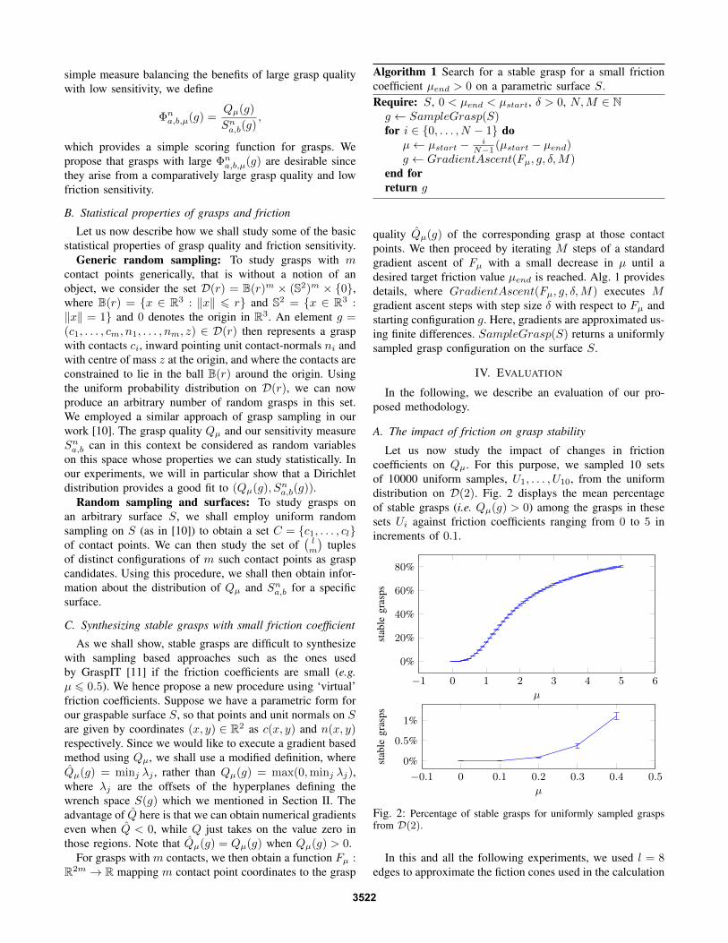
Fig. 7 shows the result of this gradient ascent on boththe bottle and the box surface by green points. We can seethat almost all the blue dots in Fig. 7 have been movedtowards the right edge of the distribution cone, indicating animprovement in Φna,b,µ(g). Fig. 8 illustrates the performanceof the gradient ascent using bar-plots, with black and bluebars showing Φna,b,µ(g) values before and after gradientascent respectively. It is worth mentioning that, looking atFig. 8, the final value of Φna,b,µ seems to bounded by similarupper bounds, both for the bottle and the box surface. Fig. 9displays two examples of gradient ascent on both surfacesand corresponding to the red dots in Fig. 7. The trajectory onthe object surface represents the location of contacts in eachiteration of the gradient ascent. Note that, if we imagine thebottle to be wet or slippery, the red grasp is intuitively lessstable than the blue grasp, which is confirmed by the graphof the grasp quality depicted next to the bottle.

0 10 20 30 400

0.2

0.4

0.6

µ

Φn a,b,µ

(g)

0 10 20 30 40 50 60 700

0.2

0.4

0.6

µ

Φn a,b,µ

(g)

Fig. 8: Results of the gradient ascent on Hna,b,µ on the bottle (top)

and the box (bottom) surface. Each bar represents a grasp sampleshown in Fig. 7. Bars are sorted in ascending order of the finalΦna,b,µ(g) values which is depicted along the vertical axis. Blackbars depict Φna,b,µ values of the original grasp samples and bluebars are values after gradient ascent.

0.2 0.4 0.6 0.8 10

0.05

0.1

0.15

0.2

0.2 0.4 0.6 0.8 10

0.1

0.2

Fig. 9: An example of gradient ascent for Φna,b,µ corresponding tothe red points in Fig. 7. The red grasps converge to the blue onesunder our gradient ascent. The trajectories are depicted as faintlines.

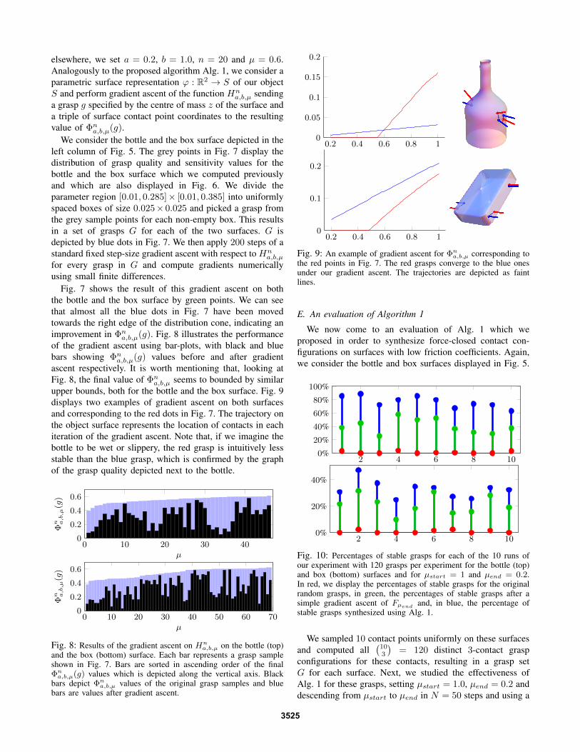
E. An evaluation of Algorithm 1

We now come to an evaluation of Alg. 1 which weproposed in order to synthesize force-closed contact con-figurations on surfaces with low friction coefficients. Again,we consider the bottle and box surfaces displayed in Fig. 5.

2 4 6 8 100%

20%

40%

60%

80%

100%

2 4 6 8 100%

20%

40%

Fig. 10: Percentages of stable grasps for each of the 10 runs ofour experiment with 120 grasps per experiment for the bottle (top)and box (bottom) surfaces and for µstart = 1 and µend = 0.2.In red, we display the percentages of stable grasps for the originalrandom grasps, in green, the percentages of stable grasps after asimple gradient ascent of Fµend and, in blue, the percentage ofstable grasps synthesized using Alg. 1.

We sampled 10 contact points uniformly on these surfacesand computed all

(103

)= 120 distinct 3-contact grasp

configurations for these contacts, resulting in a grasp setG for each surface. Next, we studied the effectiveness ofAlg. 1 for these grasps, setting µstart = 1.0, µend = 0.2 anddescending from µstart to µend in N = 50 steps and using a

3525

gradient ascent with step size δ = 0.05 and M = 40 steps periteration according to Alg. 1. We repeated this experiment 10times for each surface, resulting in the percentages of stablegrasps (Qµend

(g) > 0) depicted by blue dots in Fig. 10.To compare our result to a more straightforward approach,

we tested the alternative approach of simply performing agradient ascent of Fµend

for each grasp, and with step-sizeδ = 0.05 and for M = 200 iterations which resulted in themuch lower percentages of stable grasps depicted in green.If we simply use a sampling based approach and evaluatethe grasp quality for each grasp in our set with frictionµend, almost none of the sampled grasps had positive graspquality as indicated by red dots. Our results hence indicatethat Alg. 1 can be used to successfully synthesize stablegrasp configurations on objects with low friction coefficientsby repeating the algorithm a few times with different randomstarting grasps until a stable grasp is found.

V. CONCLUSION

Studying grasping under uncertainty is an important areain robotics [14], [15], [16], [17], [18]. While most currentstate of the art approaches concentrate on aspects of imper-fect object or robot models, we studied another fundamentalproblem in grasp synthesis in this work: the dependence ofgrasp stability on friction coefficients. We believe that thisis an important problem when robots are to operate in open-ended environments with changing conditions.

We have in particular studied the statistics of stable graspsunder changes in friction coefficients and have introduced thenotion of friction sensitivity measuring the susceptibility of agrasp’s quality to changes in friction. Furthermore, we haveproposed and evaluated two gradient ascent algorithms forsynthesizing force-closed contact configurations on paramet-ric surfaces with potentially low friction and for the synthesisof stable grasps with low friction sensitivity.

In our future work, we would like to evaluate our approachwith a real robot and study changes in friction coefficientsin a real application such as a household robot cleaningdishes which might be dirty or wet, impacting heavily onthe resulting friction properties. Further directions might also

include the study of alternative friction models and graspquality scoring functions.

REFERENCES

[1] C. Ferrari and J. Canny, “Planning optimal grasps,” IEEE ICRA, pp.2290–2295, 1992.

[2] C. Borst, M. Fischer, and G. Hirzinger, “Grasping the dice by dicingthe grasp,” in IEEE/RSJ IROS, 2003, pp. 3692–3697.

[3] A. Bicchi and V. Kumar, “Robotic grasping and contact: A review,”in IEEE ICRA, 2000, pp. 348–353.

[4] C. B. Barber, D. P. Dobkin, and H. Huhdanpaa, “The quickhullalgorithm for convex hulls,” ACM Trans. Math. Software, vol. 22,no. 4, 1996.

[5] J. Lancaster, “A review of the influence of environmental humidityand water on friction, lubrication and wear,” Tribology International,vol. 23, no. 6, pp. 371–389, 1990.

[6] F. M. Chester, “Effects of temperature on friction: Constitutive equa-tions and experiments with quartz gouge,” Journal of GeophysicalResearch, vol. 99, pp. 7247–7247, 1994.

[7] Y. Zheng and W.-H. Qian, “Coping with the grasping uncertainties inforce-closure analysis,” The Int. Journal of Robotics Research, vol. 24,no. 4, pp. 311–327, 2005.

[8] M. A. Roa and R. Suarez, “Influence of contact types and uncertaintiesin the computation of independent contact regions,” in IEEE ICRA,2011, pp. 3317–3323.

[9] Y. Zheng, M. C. Lin, and D. Manocha, “On computing reliable optimalgrasping forces,” IEEE Trans. on Robotics, vol. 28, no. 3, pp. 619–633,2012.

[10] F. T. Pokorny, K. Hang, and D. Kragic, “Grasp moduli spaces,” inProc. of Robotics: Science and Systems, Berlin, Germany, June 2013.

[11] A. Miller and P. Allen, “Graspit! a versatile simulator for roboticgrasping,” IEEE Robotics Aut. Mag., vol. 11, no. 4, pp. 110–122, 2004.

[12] T. Minka, “The fastfit matlab toolbox,” 2006. [Online]. Available:http://research.microsoft.com/en-us/um/people/minka/software/fastfit

[13] H. Chernoff and E. L. Lehmann, “The use of maximum likelihoodestimates in 2 tests for goodness of fit,” The Annals of MathematicalStatistics, vol. 25, no. 3, pp. 579–586, 1954.

[14] K. Huebner, S. Ruthotto, and D. Kragic, “Minimum volume boundingbox decomposition for shape approximation in robot grasping,” inICRA, 2008.

[15] M. Toussaint, N. Plath, T. Lang, and N. Jetchev, “Integrated motorcontrol, planning, grasping and high-level reasoning in a blocks worldusing probabilistic inference,” in IEEE ICRA, 2010, pp. 385–391.

[16] M. Przybylski, T. Asfour, and R. Dillmann, “Planning grasps forrobotic hands using a novel object representation based on the medialaxis transform,” in IEEE/RSJ IROS, 2011, pp. 1781–1788.

[17] D. Song, K. Huebner, V. Kyrki, and D. Kragic, “Learning taskconstraints for robot grasping using graphical models,” in IEEE/RSJIROS, 2010, pp. 1579–1585.

[18] M. Madry, D. Song, and D. Kragic, “From object categories to grasptransfer using probabilistic reasoning,” in IEEE ICRA, 2012, pp. 1716–1723.

3526