Friction and Heat Transfer Characteristics for Single-Phase Flow in Microchannel

Condenser Tubes

ACRCTR-78

For additional information:

Air Conditioning and Refrigeration Center University of Illinois Mechanical & Industrial Engineering Dept. 1206 West Green Street Urbana, IL 61801

(217) 333-3115

T. P. Graham and W. E. Dunn

June 1995

Prepared as part of ACRC Project 48 Analysis of Microchannel Condenser Tubes

w. E. Dunn, Principal Investigator

The Air Conditioning and Refrigeration Center was founded in 1988 with a grant from the estate of Richard W. Kritzer, the founder of Peerless of America Inc. A State of Illinois Technology Challenge Grant helped build the laboratory facilities. The ACRC receives continuing support from the Richard W. Kritzer Endowment and the National Science Foundation. The following organizations have also become sponsors of the Center.

Acustar Division of Chrysler Amana Refrigeration, Inc. Brazeway, Inc. Carrier Corporation Caterpillar, Inc. Delphi Harrison Thennal Systems E. I. du Pont de Nemours & Co. Eaton Corporation Electric Power Research Institute Ford Motor Company Frigidaire Company General Electric Company Lennox International, Inc. Modine Manufacturing Co. Peerless of America, Inc. U. S. Anny CERL U. S. Environmental Protection Agency Whirlpool Corporation

For additional iriformation:

Air Conditioning & Refrigeration Center Mechanical & Industrial Engineering Dept. University of Illinois 1206 West Green Street Urbana IL 61801

2173333115

1-..

FRICTION AND HEAT TRANSFER CHARACTERISTICS FOR SINGLE-PHASE FLOW IN MICROCHANNEL CONDENSER TUBES

Timothy Paul Graham, M.S. Department of Mechanical and Industrial Engineering

University of Illinois at Urbana-Champaign, 1995 W.E. Dunn, Advisor

An experimental study of friction and heat transfer characteristics for single-phase

flow in microchannel condenser tubes was conducted. Data were collected for the

adiabatic flow of nitrogen, and also for the diabatic flow of single-phase R134a w.ith air

in cross-flow. The nitrogen data were analyzed to obtain friction factors in the Reynolds

number range of 500-20000, and the R134a data were analyzed to obtain Nusselt

numbers in the Reynolds number ranges of 1000-7000 and 10000-70000.

Several types of microchannel tubes were considered, including those with circular,

square, enhanced square, and equilateral triangular ports. For each tube geometry,

friction factors in the laminar regime follow the known analytical solution, but the critical

Reynolds numbers for the noncircular tubes are all smaller than the value of 2100 found

for the circular-port tube. In the turbulent regime, microchannel tube friction. factors

follow a correlation for smooth tubes given by Churchill. Accordingly, there is no

evidence of surface roughness or small length scale effects. Finally, Nusselt numbers

in the range of 10000-70000, obtained from superheated vapor data, are within 10% of

the correlation given by Gnielinski. The heat transfer data in the range of 1000-7000,

obtained from subcooled liquid, are inconclusive.

iii

TABLE OF CONTENTS

~"

fawl LIST OF TABLES ................................ ................................................... ................ vii

LIST OF FIGURES ................................................................................................ viii

NOMENCLATURE .. .............................. ................................................................. x

1 . INTRODUCTION ............. ... ................... ... .......... ........ ................ .... ......... ...... 1

1.1 Microchannel Condenser Description ......................•... ...... .................... 1

1.2 Objedives.......... ........ ......................... ........ .... ......................... ..... ......... 2

2. LITERATURE REViEW................ ............ .... .......................................... ....... 4

2.1 Introdudion ................................................................................ ~........... 4

2.2 Fridion Fadors for Dud Flow ................................................................ 4

2.2.1 Laminar Flow ............... ........ ............ ...... .......... ......... ......... ....... 6

2.2.2 Turbulent Flow ................................ .......................................... 8

2.3 Nusselt Numbers for Dud Flow................................ ...... ................... .... 14

2.3.1 Laminar Flow ................................ ................................. ........... 15

2.3.2 Turbulent Flow.......... ...................... ......................................... 16

2.4 Compressibility Effects ................................ .......................................... 21

2.5 Small Length Scale Effects .................................................................... 21

3. EXPERIMENTAL FACILITIES ....................................................................... 23

3.1 Nitrogen Test Facility ............................................................................. 23

3.1.1 Nitrogen Supply ........................ ................ ............. ................... 24

3.1.2 Mass Flow Rate Measurement ............... .... .......... ................... 25

3.1.3 Tempering Coil ......................................................................... 26

3.1.4 Pressure Regulation .. .............................. ............. .................... 26

3.1.5 Transition Sedion ............ .................................. .......... ............. 27

3.1.6 Pressure Measurement ..... ........................... ............................ 28

3.1.7 Temperature Measurement ...................................................... 28

3.2 R134a Test Facility ................................................................................ 29

3.2.1 . Refrigerant Loop ...... ................. ..... .... .... .......... ................. ....... 29

3.2.2 Air Loop .................................................................................... 31

v

4. EXPERIMENTAL PROCEDURE AND RESULTS ......................................... 32

4.1 Data Collection .......................................... ;........................................... 32 ~.:

4.1.1 Microchannel Tube Test Sections ................................ i •••••••• ~.. 32

4.1.2 Nitrogen Test Facility Data Collection ....................... ~.............. 36

·4.1.3 R 134a Test Facility Data Collection ......................................... 37

4.2 Data Reduction ...................................................................................... 38

4.2.1 Nitrogen Test Facility Entrance Coefficients ............................ 38

4.2.2 Flow Analysis for Friction Factors and UA Values ................... 42

4.2.3 Integration of the Conservation Equations ............................... 47

4.2.4 Wilson Plot Analysis for Nusselt Numbers ........... .................... 50

4.3 Results ..... .... ....... ................ .... ................................................ ............... 52

4.3.1 Friction Factors from the Nitrogen Tests .................................. 52

4.3.2 Nusselt Numbers from the R134a Tests .................................. 62

5. PROJECT SUMMARY AND CONCLUSIONS ............................................... 66

5.1 Summary of Results .............................................................................. 66

5.2 Recommendations for Future Research .......... ...... ...... .... ...... ... ............. 67

APPENDIX A

APPENDIXB

REFERENCES

ENLARGED PORT IMAGES ...................................................... .

COMPUTER PROGRAM FOR DATA REDUCTION ................. .

vi

69

73

89

Table 2.1

Table 2.2

Table 4.1

Table 4.2

LIST OF TABLES

1>:

Laminar flow solutions for constant-area ducts. . ........................... .

Length scales for constant-area ducts. . ....................................... ..

Measured free-flow dimensions for the microchannel tube test sections. . ....................................................................................... .

Geometric parameters for the microchannel tube test sections.

vii

easm 7

13

35

54

LIST OF FIGURES

fage.

Figure 1.1 Microchannel tube schematic. ....................................................... 2

Figure 3.1 Nitrogen Test Facility schematic. ................................................... 24

Figure 3.2 NTF transition section. ................................................................... 27

Figure 3.3 . R134a Test Facility schematic ....................................................... 30

Figure 4.1 Circular-port tube. .. .............................. .................. .......... ...... ........ 33

Figure 4.2 Square-port tube. ........................................................................... 33

Figure 4.3 Triangular-port tube. ...... ............ ...... ............ .................... .............. 33

Figure 4.4 Small square-port tube. ................................ ................................. 33

Figure 4.5 Enhanced square-port tube. .......................................................... 34

Figure 4.6 Enlarged triangular-port image. ..................................................... 35

Figure 4.7 Dimensionless pressure drop versus length for the circular-port tubes. ............................................................................................. 39

Figure 4.8 NTF entrance coefficients for the circular-port test section. ........... 40

Figure 4.9 NTF entrance coefficients for the square-port test section. ........... 41

Figure 4.10 NTF entrance coefficients for the triangular-port test section. ....... 41

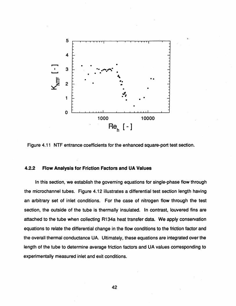
Figure 4.11 NTF entrance coefficients for the enhanced square-port test section. .......................................................................................... 42

Figure 4.12 Differential section of a microchannel tube. .... ...... .......... ............... 43

Figure 4.13 Wilson plot for the circular-port test section. .................................. 52

Figure 4.14 Circular-port results using the measured hydraulic diameter. ....... 53

Figure 4.15 Friction factors for the circular-port test section. ............................ 55

Figure 4.16 Friction factors for the square-port test section. ............................ 56

Figure 4.17 Alternative length scales for the square-port test section. ............. 57

Figure 4.18 Friction factors for the triangular-port test section. 58

viii

Figure 4.19 Alternative length scales for the triangular-port test section. ... ...... 58

Figure 4.20 Friction factors for the small square-port test section . ............... t... 59

Figure 4.21 Alternative length scales for the small square-port test section. ... 60

Figure 4.22 Friction factors for the enhanced square-port test section. ............ 61

Figure 4.23 Alternative length scales for the enhanced square-port test section. . ....... :................................................................................. 61

Figure 4.24 Nusselt numbers for the circular-port test section. ........................ 63

Figure 4.25 Nusselt numbers for the square-port test section. ......................... 63

Figure 4.26 Nusselt numbers for the triangular-port test section. ..................... 64

Figure 4.27 Nusselt numbers for the small square-port test section. ............... 64

Figure 4.28 Nusselt numbers for the enhanced square-port test section. .. ...... 65

Figure A.1 Enlarged circular-port image. ......................................................... 69

Figure A.2 Enlarged square-port image. ......................................................... 70

Figure A.3 Enlarged small square-port image. ............ .... ..... ...... ..... ...... .......... 71

Figure A.4 Enlarged enhanced square-port image. ........................................ 72

ix

English Symbols

A

Cair

Cmax

Cmin

Cret

Cp,air

Cp,ref

D

D:" IC

D~

to

to,cf

to,s

h

NOMENCLATURE

free-flow area

cross sectional area

heat capacity rate of the air

maximum heat capacity rate

minimum heat capacity rate

heat capacity rate of the refrigerant

specific heat of the air at constant pressure

specific heat of the refrigerant at constant pressure

tube diameter

critical friction diameter

hydraulic diameter

average of inscribed circle and circumscribed circle diameters

laminar equivalent diameter

nondimensional equivalent diameter, Deq / Dh

nondimensional Ric" diameter, Die / Dh

nondimensionallaminar equivalent diameter, Die / Dh

Darcy friction factor

modified Darcy friction factor from the critical friction method

smooth tube Darcy friction factor

force in the. axial direction

heat transfer coefficient

average refrigerant-side heat transfer coefficient

x

A

h

k

rh

Np

Nu

NUcr

NUexpt

NUpred

Nus

Nu'

A n

p

Ap

fluid enthalpy

. thermal conductivity of the fluid

laminar friction constant

Nitrogen Test Facility entrance coefficient

pressure drop number

tube length

characteristic length

mass flow rate

number of microchannel ports

Nusselt number based on the characteristic length, hLc / k

critical Nusselt number based on tube diameter

experimental value of the Nusselt number

fully developed Nusselt number

critical Nusselt number based on hydraulic diameter

Nusselt number for axially constant wall heat flux, circumferentially constant wall temperature

Nusselt number for uniform wall heat flux

predicted value of the Nusselt number

smooth tube Nusselt number

Nusselt number for uniform wall temperature

average Nusselt number

average Nusselt number for constant wall temperature

modified Nusselt number from the critical friction method

normal unit vector

fluid pressure

incremental pressure drop

xi

p

Pr

q

. q"

Rair

Rref

Rtot

RWaJl

Re

Reef

Reer

Reh

Reh.er

Reic

Rele

Re'

St.ref

Sp.ref

T

T air.i

Tm

Tref.i

Tw

U

Ufd

wetted perimeter

Prandtl number of the fluid, CpJ! / k

heat transfer rate

heat transfer rate per unit area

air-side thermal resistance

refrigerant-side thermal resistance

total thermal resistance

thermal resistance of the wall

Reynolds number based on tube diameter, pVD / J!

Reynolds number based on critical friction diameter, pVDef / J!

critical Reynolds number based on tube diameter

Reynolds number based on hydrauliC diameter, pVDh / J!

critical Reynolds number based on hydrauliC diameter

Reynolds number based on "ic" diameter, pVDic / J!

Reynolds number based on laminar equivalent diameter, pVDle / J!

modified Reynolds number from the critical friction method

surface area of the fins in contact with the refrigerant

primary surface area in contact with the refrigerant

fluid temperature

inlet temperature of the air

mean fluid temperature

inlet temperature of the refrigerant

wall temperature

axial velocity

fully developed axial velocity

xii

um

UA

V

V

x

Ax

Greek Symbols

a

£

Il

Ilw

11f

P

mean axial velocity

overall thermal conductance

average fluid velocity

velocity vector

axial coordinate

incremental tube length

kinetic-energy correction factor

momentum-flux correction factor

effective surface roughness

dynamic viscosity of the fluid

dynamic viscosity evaluated at the wall temperature

fin efficiency

fluid density

perimeter-average wall shear stress

xiii

~.:

1. INTRODUCTION

Microchannel heat exchanger technology1 is currently being utilized for the

construction of compact air conditioning condensers. Microchannel condensers offer

improved thermal performance and tremendous design flexibility, but the physics

governing their performance are not well understood. Accordingly, an investigation into

the fluid flow and heat transfer characteristics of the microchannel tubes is necessary

for condenser optimization.

This document presents the results obtained from an investigation of friction and

heat transfer characteristics for single-phase flow in microchannel tubes. These results

are part of a more extensive study which includes full condenser modeling and two­

phase flow modeling.

1.1 Microchannel Condenser Description

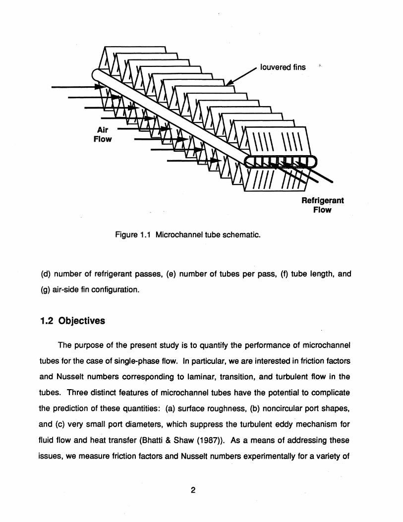
Figure 1.1 is a schematic of a single microchannel tube with a set of louvered fins

designed to enhance air-side heat transfer. The microchannel tubes are aluminum

extrusions having a particuar number of ports and a specific type of port geometry. A

variety of port geometries are available, including circles, squares, and triangles. The

fins are also aluminum, and they are attached to the tubes through a brazing process.

A full microchannel condenser consists of several tubes which are brazed to

headers on either side. The tubes are arranged in a staCk, and the air-side fins are

nestled between them. The refrigerant is circuited by baffles in the headers, resulting in

several passes with multiple tubes per pass. Thus, the following design options are

available: (a) number of tubes, (b) number of ports per tube, (c) port size and geometry,

Microchannel heat exchanger technology is the subject of United States and foreign patents applied for and issued to Modine Manufacturing Company, Racine, Wisconsin, USA. Current United States patents include 4,615,385,4,688,311 and 4,998,580.

1

Air Flow

Figure 1.1 Microchannel tube schematic.

louvered fins

Refrigerant Flow

(d) number of refrigerant passes, (e) number of tubes per pass, (f) tube length, and

(g) air-side fin configuration.

1.2 Objectives

The purpose of the present study is to quantify the performance of microchannel

tubes for the case of single-phase flow. In particular, we are interested in friction factors

and Nusselt numbers corresponding to laminar, transition, and turbulent flow in the

tubes. Three distinct features of microchannel tubes have the potential to complicate

the prediction of these quantities: .(a) surface roughness, (b) noncircular port shapes,

and (c) very small port diameters, which suppress the turbulent eddy mechanism for

fluid flow and heat transfer (Bhatti & Shaw (1987». As a means of addressing these

issues, we measure friction factors and Nusselt numbers experimentally for a variety of

2

port geometries. Using these results, we compare the performance of microchannel

tubes to that of conventional tubes. ;>- ..

Two test facilities are used to collect experimental data for a single microchannel

tube. The first is a nitrogen facility, which yields adiabatic flow data used to determine

friction factors. The second is an R134a facility, which circulates refrigerant through the

tube and air in cross flow (see Figure 1.1). Data from the R134a facility are used to

determine refrigerant-side Nusselt numbers. For each case, the methods used to

reduce the data are discussed in detail.

3

2. LITERATURE REVIEW

2.1 Introduction

The study of fluid flow and forced convection heat transfer in constant-area ducts is

a classical problem with a wide variety of practical applications. Consequently, there is

an extensive amount of literature devoted to the subject. Researchers usually quantify

friction and heat transfer for duct flow in terms of the nondimensional friction factor and

Nusselt number. Use of these nondimensional quantities allows one to apply the values

to dynamically similar flows.

This review presents results for single-phase duct flow that are applicable to

microchannel condenser tubes. The microchannel ports are considered to be straight

passages with axially uniform cross sections. The walls of the tube are assumed to be

nonporous, rigid, and stationary. A variety of port geometries are typical, including

those with circular, square, and triangular cross sections.

The expressions presented hereafter apply to steady, incompressible flow of

Newtonian fluids with constant properties. The influence of body forces and natural

convection are neglected. Also neglected are heat sources, viscous dissipation, and

axial conduction in the fluid. The effects of compressibility and small tube sizes are

subsequently considered.

2.2 Friction Factors for Duct Flow

Most important for engineering calculations is a knowledge of friction factors for

duct flow (Eckert & Irvine (1957)). Several definitions of the friction factor are found in

the literature, including the Darcy friction factor (White (1987)):

f - 4'tw 0-1

_pV2 2

4

(2.1 )

where tw is the perimeter-average wall shear stress, p is the fluid density, and V is the

fluid velocity. The Darcy friction factor represents the ratio of the wal.1 shear stress to

the kinetic energy per unit volume of the flow.

Because the wall shear stress is related to the velocity profile, the friction factor is

determined by solving the continuity and momentum equations for a given flow.

Consequently, the value of the friction factor strongly depends on the Reynolds number.

Once the friction factor is determined, the pressure drop across the duct is found from a

momentum balance.

In the fully developed region of the duct, the velocity profile is invariant at any flow

cross section (Shah & London (1978)). Therefore the wall shear stress and the friction

factor are constant in the axial direction. The momentum balance in this region has the

following form:

(2.2)

where Ap is the incremental pressure drop, Ax is the incremental length, and Dh is the

hydraulic diameter of the duct.

In the hydrodynamic entrance region, there is an increase in the wall shear stress

and a change in the momentum flux due to the developing velocity profile. These

entrance effects result in a pressure drop that is greater than that which would exist for

fully developed flow. When calculating the overall pressure drop, it is necessary to

account for these effects. Shah and Bhatti (1987) define the pressure drop number K­

so that the overall momentum balance becomes

5

Ap L 1 =fo-D +Koo _pV2 h 2

(2.3)

where L is the length of the duct and fo is the fully developed Darcy friction factor.

2.2.1 Laminar Flow

The continuity and momentum equations are fairly simple for laminar duct flow.

Therefore, analytical solutions for the friction factor and the pressure drop number are

known for a variety of cases. Shah and London (1978) compiled an exhaustive

monograph of the available solutions for laminar fluid flow and forced convection heat

transfer in ducts. They present their results in numerical, graphical, and tabular forms.

For fully developed flow, solution of the momentum equation yields

(2.4)

. where Kf is a constant depending on the cross-sectional geometry, and Reh is the

Reynolds number based on the hydraulic diameter. Table 2.1 lists values of Kf for a

variety of duct geometries.

Values for the pressure drop number are determined by solving the Navier-Stokes

equations in the hydrodynamic entrance region. However, very few closed-form

solutions exist because the equations are nonlinear. For ducts with circular cross

sections, the analysis of Chen (1973) results in the following expression:

38 Koo = 1.20+­

Re

6

(2.5)

Table 2.1 Laminar flow solutions for constant-area ducts.

Geometry Kf NUT NUH1 NUH2

0 64.000 3.657 4.364 4.364

circle

D 56.908 2.976 3.608 3.091

square

~ 53.332 2.470 3.111 1.892 equilateral

triangle

c=J~ 62.192 3.391 4.123 3.017 a

rectangle: pia =1/2

I I ~ a

72.932 4.439 5.331 2.930 rectangle: pia =1/4

where Re is the Reynolds number based on the diameter. Equation 2.5 assumes a

uniform velocity profile at the inlet. For noncircular ducts, Shah and London (1978)

present results from a number of investigators in graphical form. In particular, the

values of Miller and Han (1971) for rectangular and equilateral triangular ducts are in

closest agreement with experimental values.

In addition to solving the Navier-Stokes equations, approximate analytical methods

are used to calculate pressure drop number. These methods generally incorporate

boundary layer simplifications and assume a uniform velocity profile at the inlet.

7

Lundgren, Sparrow, and Starr (1964) used this approach to develop the following

expression for ducts of arbitrary cross section:

(2.6)

where At; is the cross-sectional area of the duct, Ufd is the fully developed axial velocity,

and Urn is the mean axial velocity. Shah and London (1978) point out that values

obtained from this equation are generally higher than experimental values.

2.2.2 Turbulent Flow

It is well known that flow in a duct becomes turbulent above some critical value of

the Reynolds number. The structure of the flow field is extremely complicated in this

regime, making it impossible to solve the governing equations analytically.

Consequently, researchers have focused on the development of semitheoretical and

experimental correlations for the friction factor. All of the correlations presented in this

section assume flows with fully developed velocity profiles.

The most extensive studies of turbulent duct flow involve those with circular cross

sections. The lower limit of the critical Reynolds number Recr is widely accepted as

2300 for these ducts, although Obot (1988) reports a value of 2115 based on data from

several sources. Transition to turbulent flow occurs over a range of Reynolds numbers,

typically 2300 ~ Re < 4000. Churchill (1977a) used the numerical results of Wilson and

Azad (1975) to derive an empirical equation for the transitional regime:

(2.7)

8

For turbulent flow in a smooth circular duct, the Prandtl-Karman-Nikuradse (PKN)

correlation is regarded as the most accurate (Bhatti & Shah (1987)):

--,1-= 0.8686 In(Re..Jfo )-0.9967 . -vfo

(2.8)

This expression is based on the logarithmic velocity law and the experimental data of

Nikuradse (1932) for Re > 4000. Various investigators recast Equation 2.8 so that the

friction factor appears explicitly.

For the case of a rough circular duct, Nikuradse (1933) determined an asymptotic

expression for the fully rough range:

~;D =0.8687 In( 3.707~) (2.9)

where 0 is the diameter of the duct, and £ is the effective surface roughness. Equation

2.9 shows that the friction factor has no Reynolds number dependence when the flow is

fully rough.

Colebrook (1939) combined Equations 2.8 and 2.9 to provide an expression for

the transitionally rough range:

1 =1.74-0.8686 In(~+ 18.7 J To 0 Re~fD (2.10)

which serves as the basis of the well known Moody chart. In a similar fashion, Churchill

(1977a) combined expressions for the laminar, transition, and turbulent regimes to

obtain the following equation:

9

fo 8 1· [12 J1/12

8 = (Re) + (A+B)3/2 (2.11 )

where

and

Equation 2.11 is convenient because the friction factor appears explicitly and it is valid

for the full range of Reynolds numbers.

For turbulent flow in noncircular ducts, the standard procedure is to use the

hydraulic diameter in conjunction with the circular tube expressions. This method is

based on the assumption that ducts with identical hydraulic diameters have the same

bulk flow properties. Ahmed and Brundrett (1970) say that for the assumption to hold,

the isovels must be parallel to the boundary and they must satisfy the logarithmic

velocity law up to the corner bisector. In actual practice, the log law is satisfied only in

regions very close to the wall due to the presence of secondary mean flows

(Leutheusser (1963)). It is not surprising, therefore, that use of the hydraulic diameter

for ducts with sharp corners can lead to large errors in the calculated friction factors.

For this reason, alternative length scales are used to obtain better values for specific

duct geometries.

For smooth rectangular ducts, Jones (1976) suggests that the proper length scale

is one which provides similarity between circular and rectangular ducts in laminar flow.

This length scale is found by modifying the hydraulic diameter so that the laminar friction

factor relation becomes identical to that for a circular duct. The resulting laminar

equivalent diameter Ole is given by

10

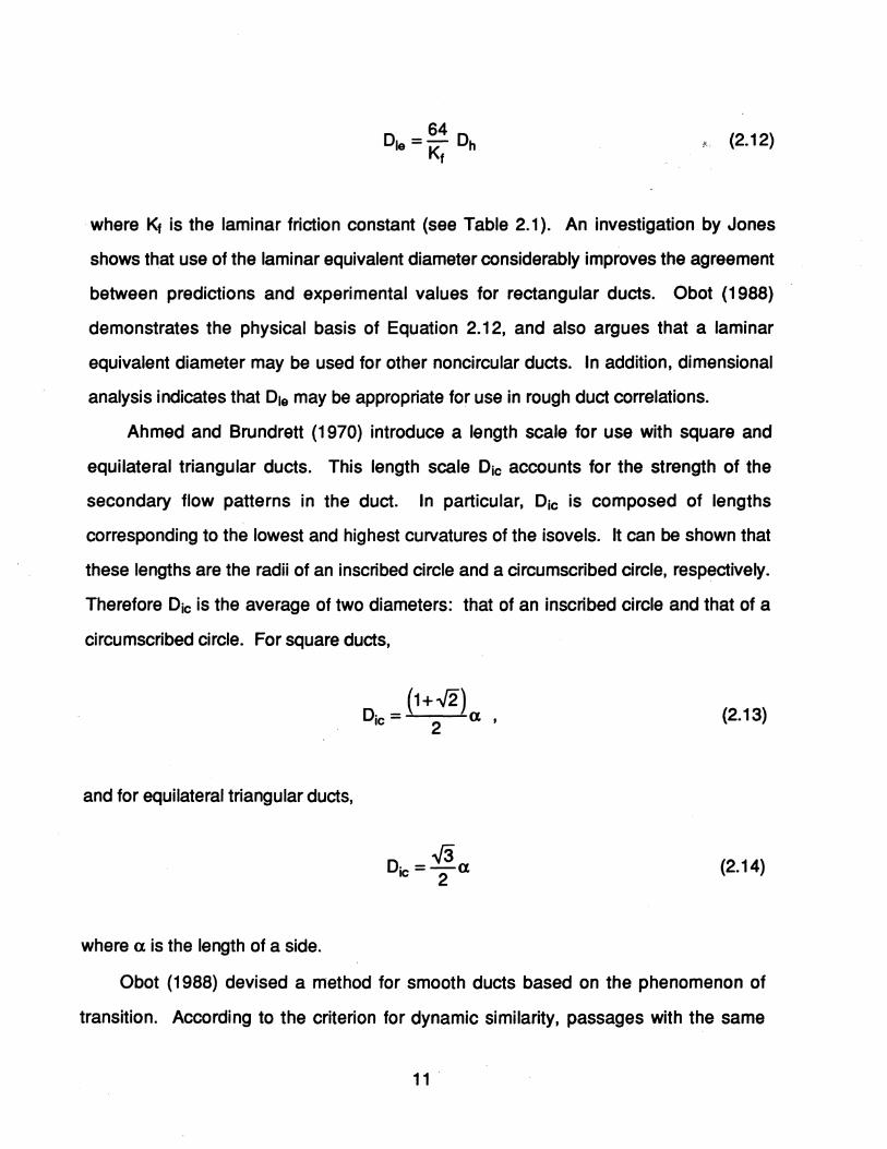
". (2.12)

. where Kf is the laminar fridion constant (see Table 2.1). An investigation by Jones

shows that use of the laminar equivalent diameter considerably improves the agreement

between predictions and experimental values for redangular duds. Obot (1988)

demonstrates the physical basis of Equation 2.12, and also argues that a laminar

equivalent diameter may be used for other noncircular duds. In addition, dimensional

analysis indicates that Ole may be appropriate for use in rough dud correlations.

Ahmed and Brundrett (1970) introduce a length scale for use with square and

equilateral triangular duds. This length scale Dic accounts for the strength of the

secondary flow patterns in the dud. In particular, Dic is composed of lengths

corresponding to the lowest and highest curvatures of the isovels. It can be shown that

these lengths are the radii of an inscribed circle and a circumscribed circle, respedively.

Therefore Die is the average of two diameters: that of an inscribed circle and that of a

circumscribed circle. For square dudS,

and for equilateral triangular duds,

where a is the length of a side.

.J3 Dic=-a 2

(2.13)

(2.14)

Obot (1988) devised a method for smooth duds based on the phenomenon of

transition. According to the criterion for dynamic similarity, passages with the same

11

critical friction factor and critical Reynolds number will possess identical turbulent

frictional pressure coefficients (Obot (1988». The data presented by Obot reveals that

the critical friction factor assumes a nearly universal value for all duct geometries.

Consequently, the proper choice for a length scale is one which makes the critical

Reynolds number identical to that for a circular duct. The resuH is the critical friction

diameter Dct :

D - Recr D ct - Re h

h,cr (2.15)

where Recr pertains to a circular. duct and Reh,cr pertains to the noncircular duct in

question. It is reasonable to assume that the critical friction diameter may be used for

rough channels. Furthermore, there is no need to correct for secondary flows because

the method ensures dynamic Similarity. In a comparison with the method of Jones

(1976), Obot demonstrates that the critical friction diameter is nearly identical to the

laminar equivalent diameter. Obot also mentions that the use of Dct hinges upon the

availability of transition data; whereas the use of Die requires analytical solutions for

laminar flow.

Table 2.2 compares the various length scales for several duct geometries. The

hydraulic diameter is used to nondimensionalize the length scales, as indicated by the

"*" superscript. Accordingly, the nondimensional form of a length scale is used as a

correction factor for the hydraulic diameter.

For turbulent duct flow, entrance effects are commonly neglected in the calculation

of frictional pressure drop. This action is justified because the hydrodynamic entrance

length is characteristically much shorter than the corresponding length for laminar flow

(Bhatti & Shah (1987». In any case, several investigators present pressure drop

numbers for specific duct geometries. Most of the analyses are based on the

12

Table 2.2 Length scales for constant-area ducts.

~.:

Geometry Dh Dh D~ D~

8 ° 1.0 1.0 1.0

circle

D a 1.0 1.125 1.207

a square

~ .J3 1.0 1.200 1.500 -a

a 3 equilateral

triangle

D~ 2 -a 1.0 . 1.029 1.126 a 3

rectangle: J31a =1/2

I I ~ 2 a -a 1.0 0.878 1.090 rectangle: 5 J31a =1/4

momentum integral method, assuming a uniform velocity at the inlet and a power-law

velocity profile within the boundary layer. Zhi-qing (1982) used this procedure to find a

Koo value of 0.07 for circular pipes. For rectangular ducts of infinite width, Eckert and

Irvine (1957) found a Koo value of 0.045 assuming a 7th-power law for the velocity

profile. Bhatti and Shah (1987) present values graphically for a variety of duct

geometries. In all cases, the values of K- appear to be very small compared to those

for laminar flow.

13

2.3 Nusselt Numbers for Duct Flow

Heat transfer calculations for duct flow are generally performed using an

appropriate heat transfer coefficient. The nondimensional form of the heat transfer

coefficient is known as the Nusselt number:

Nu= hLc k

(2.16)

where h is the heat transfer coefficient, k is the thermal conductivity of the fluid, and Lc

is the characteristic length of the duct. For the case of laminar flow, the hydraulic

diameter is used as the characteristic length. If the flow is turbulent, other length scales

are used to obtain more accurate correlations (see Section 2.3.2). The Nusselt number

represents the ratio of conductive thermal resistance to convective resistance.

Since the heat transfer coefficient is related to the temperature profile in the fluid,

the Nusselt number is found by solving the conservation equations. The value of the

Nusselt number is therefore highly dependent on the flow conditions for a given

situation. Fortunately, the energy equation is decoupled from the Navier-Stokes

equations for incompressible flow with constant properties. Once the Nusselt number is

determined, the heat transfer rate is calculated from Newton's law of cooling:

(2.17)

where T w is the interior surface temperature of the duct, and T m is the mean

temperature of the fluid.

Flow in a duct is said to be fully developed when both the velocity profile and the

relative shape of the temperature profile are invariant in the axial direction. In contrast,

14

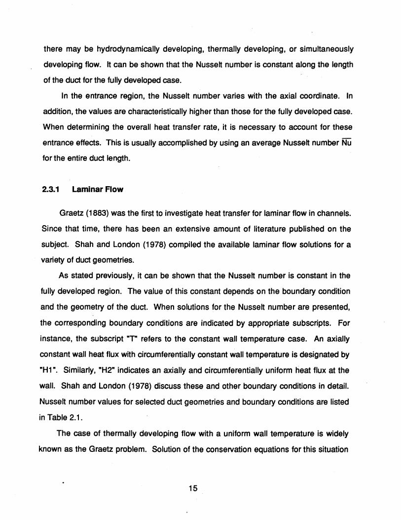
there may be hydrodynamically developing, thermally developing, or simultaneously

developing flow. It can be shown that the Nusselt number is constant along the length

of the duct for the fully developed case.

In the entrance region, the Nusselt number varies with the axial coordinate. In

addition, the values are characteristically higher than those for the fully developed case.

When determining the overall heat transfer rate, it is necessary to account for these

entrance effects. This is usually accomplished by using an average Nusselt number Nu

for the entire duct length.

2.3.1 Laminar Flow

Graetz (1883) was the first to investigate heat transfer for laminar flow in channels.

Since that time, there has been an extensive amount of literature published on the

subject. Shah and London (1978) compiled the available laminar flow solutions for a

variety of duct geometries.

As stated previously, it can be shown that the Nusselt number is constant in the

fully developed region. The value of this constant depends on the boundary condition

and the geometry of the duct. When solutions for the Nusselt number are presented,

the corr:esponding boundary conditions are indicated by appropriate subscripts. For

instance, the subscript "T" refers to the constant wall temperature case. An axially

constant wall heat flux with circumferentially constant wall temperature is designated by

"H1". Similarly, "H2" indicates an axially and circumferentially uniform heat flux at the

wall. Shah and London (1978) discuss these and other boundary conditions in detail.

Nusselt number values for selected duct geometries and boundary conditions are listed

in Table 2.1.

The case of thermally developing flow with a uniform wall temperature is widely

known as the Graetz problem. Solution of the conservation equations for this situation

15

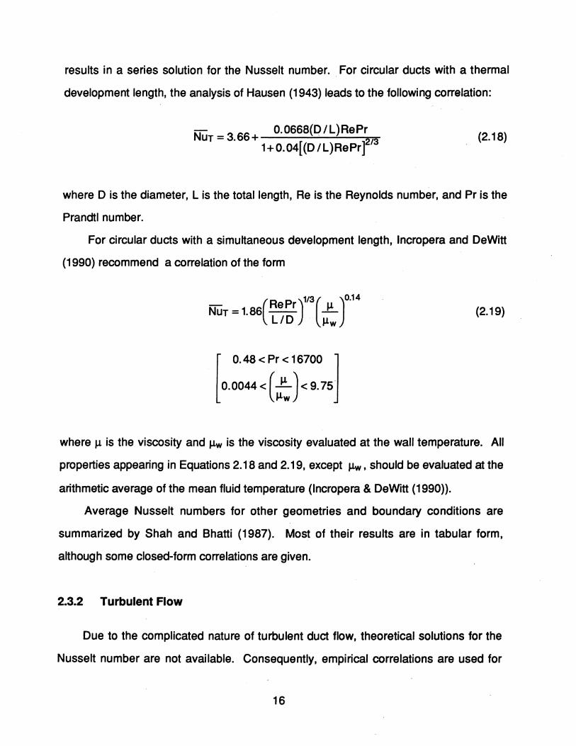
results in a series solution for the Nusselt number. For circular ducts with a thermal

development length, the analysis of Hausen (1943) leads to the following correlation:

NUT = 3.66+ 0.0668(q/L)RePr 1+0.04[(D IL)RePrf/3

(2.18)

where D is the diameter, L is the total length, Re is the Reynolds number, and Pr is the

Prandtl number.

For circular ducts with a simultaneous development length, Incropera and DeWitt

(1990) recommend a correlation of the form

_ (Repr)1/3( fl )0.14 NUT = 1.86 -- --

LID flw

[ 0.48 < Pr < 16700 ]

0.0044 < (:..) < 9.75

(2.19)

where fl is the viscosity and flw is the viscosity evaluated at the wall temperature. All

properties appearing in Equations 2.18 and 2.19, except J.1w, should be evaluated at the

arithmetic average of the mean fluid temperature (Incropera & DeWitt (1990)).

Average Nusselt numbers for other geometries and boundary conditions are

summarized by Shah and Bhatti (1987). Most of their results are in tabular form,

although some closed-form correlations are given.

2.3.2 Turbulent Flow

Due to the complicated nature of turbulent duct flow, theoretical solutions for the

Nusselt number are not available. Consequently, empirical correlations are used for

16

engineering calculations. The results presented in this section are valid for an arbitrary

thermal boundary condition, provided that the Prandtl number is greater than-0.5. The

basis of this assumption is that high-Pr fluids have a thermal resist~nce that is very

close to the wall, yielding a temperature profile that is essentially flat over most of the

cross section (Bhatti & Shah (1987)).

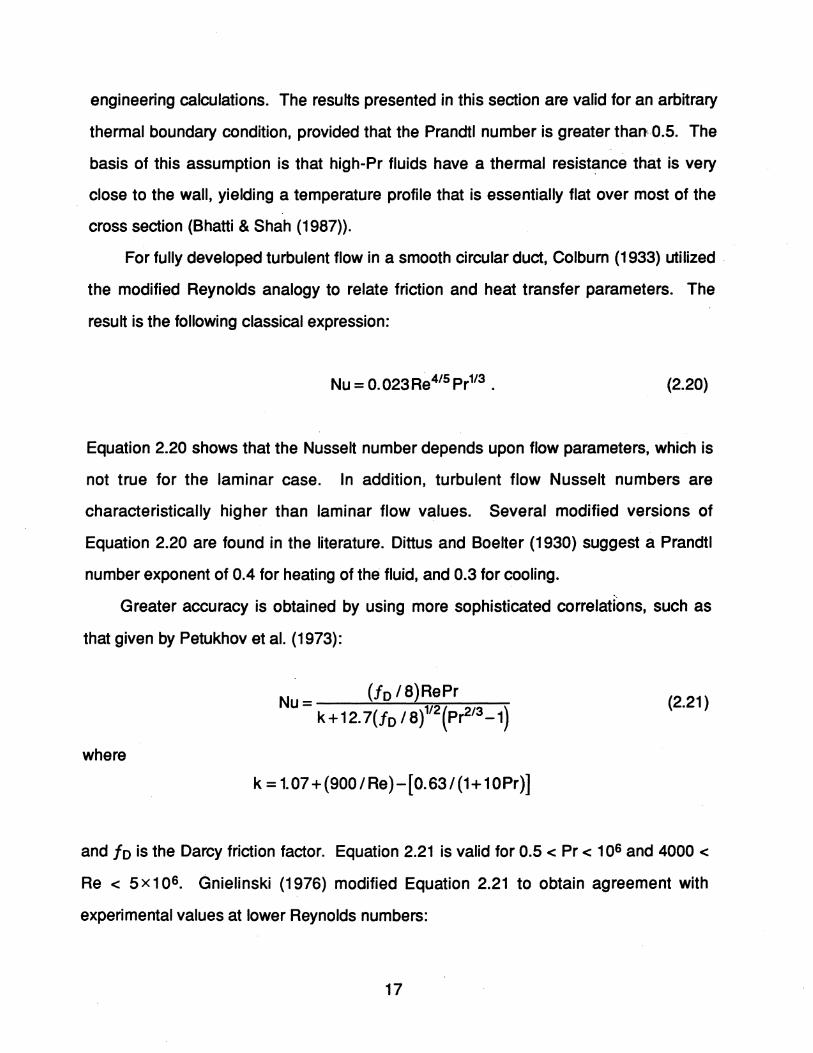
For fully developed turbulent flow in a smooth circular duct, Colburn (1933) utilized .

the modified Reynolds analogy to relate friction and heat transfer parameters. The

result is the following classical expression:

(2.20)

Equation 2.20 shows that the Nusselt number depends upon flow parameters, which is

not true for the laminar case. In addition, turbulent flow Nusselt numbers are

characteristically higher than laminar flow values. Several modified versions of

Equation 2.20 are found in the literature. Dittus and Boelter (1930) suggest a Prandtl

number exponent of 0.4 for heating of the fluid, and 0.3 for cooling.

Greater accuracy is obtained by using more sophisticated correlations, such as

that given by Petukhov et al. (1973):

Nu - (fo 18)RePr - k+ 12. 7(fo 18)1/2(pr2/3 _1)

(2.21 )

where

k = 1.07 + (900 I Re)-[0.63/(1+ 10Pr)]

and fo is the Darcy friction factor. Equation 2.21 is valid for 0.5 < Pr < 106 and 4000 <

Re < 5x 106• Gnielinski (1976) modified Equation 2.21 to obtain agreement with

experimental values at lower Reynolds numbers:

17

N _ (to /8)(Re-1000}Pr u - 1+12. 7(Jo /8)1/2(pr2/3_1) .

}. (2.22)

Equation 2.22 is valid for 0.5 < Pr < 2000 and 2300 < Re < 5x106• When applying

these correlations, it is necessary to provide an appropriate value for the friction factor.

The authors use an explicit relation given by Filonenko (1954) for this purpose:

to = (0.79 InRe - 1.64r2 . (2.23)

Friction factor values obtained from this expression are within 2% of those given by the

PKN correlation (Equation 2.8).

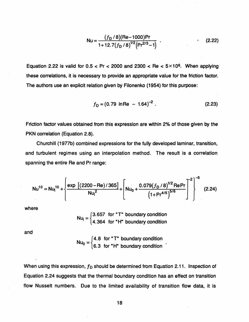
Churchill (1977b) combined expressions for the fully developed laminar, transition,

and turbulent regimes using an interpolation method. The result is a correlation

spanning the entire Re and Pr range:

N 10_N 10 !exp [(2200-Re}/365] [N 0.079(tO/8)1/2ReprJ2/-5 u - ul + 2 + Uo + 5/6

NUl (1+pr4/5 )

where

and

Nu = {3.657 for "T" boundary condition I 4.364 for" H" boundary condition

N _ {4. 8 for" T" boundary condition Uo - 6.3 for" H" boundary condition

(2.24)

When using this expression, fo should be determined from Equation 2.11. Inspection of

Equation 2.24 suggests that the thermal boundary condition has an effect on transition

flow Nusselt numbers. Due to the limited availability of transition flow data, it is

18

inconclusive as to whether or not this effect actually exists. Gnielinski (1976) does not

address this issue with regard to Equation 2.22. ~ ..

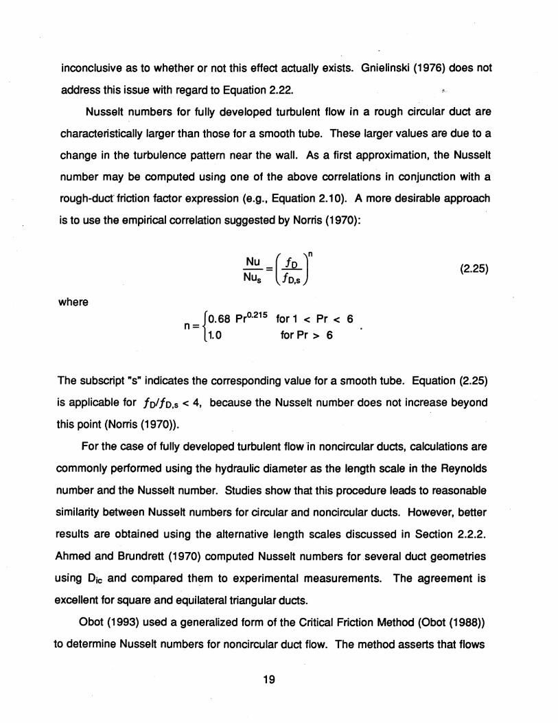
Nusselt numbers for fully developed turbulent flow in a rough circular duct are

characteristically larger than those for a smooth tube. These larger values are due to a

change in the turbulence pattern near the wall. As a first approximation, the Nusselt

number may be computed using one of the above correlations in conjunction with a

rough-duct· friction factor expression (e.g., Equation 2.10). A more desirable approach

is to use the empirical correlation suggested by Norris (1970):

( )" Nu = to Nus to,s

(2.25)

where

n = {0.68 PrO.215 for 1 < Pr < 6 1.0 for Pr > 6

The subscript "s" indicates the corresponding value for a smooth tube. Equation (2.25)

is applicable for folio,s < 4, because the Nusselt number does not increase beyond

this point (Norris (1970)).

For the case of fully developed turbulent flow 'in noncircular ducts, calculations are

commonly performed using the hydraulic diameter as the length scale in the Reynolds

number and the Nusselt number. Studies show that this procedure leads to reasonable

similarity between Nusselt numbers for circular and noncircular ducts. However, better

results are obtained using the alternative length scales discussed in Section 2.2.2.

Ahmed and Brundrett (1970) computed Nusselt numbers for .several duct geometries

using Die and compared th~m to experimental measurements. The agreement is

excellent for square and equilateral triangular ducts.

Obot (1993) used a generalized form of the Critical Friction Method (Obot (1988))

to determine Nusselt numbers for noncircular duct flow. The method asserts that flows

19

in circular and noncircular ducts can be dynamically similar only if the critical parameters

are identical. This condition is satisfied by modifying RE!h and NUh as follows: ".

Re' = ( Reer J Reh Reh,er

(2.26)

(2.27)

where Reer and NUer pertain to a circular duct. These modified parameters should be

used in conjunction with an appropriate circular tube correlation (e.g., Equation 2.22).

As indicated by Equations 2.26 and 2.27, the appropriate length scales for the Reynolds

number and Nusselt number may be different for a given noncircular duct.

When calculating the overall heat transfer rate for turbulent duct flow, the following

expression is often used to account for entrance effects:

Nu =1+ C Nutd (L/Dtt)"

(2.28)

where NUfd is the value of the Nusselt number in the fully developed region, and all

properties are evaluated at the mean fluid temperature (Incropera & DeWitt (1990)).

The coefficient C and the exponent n depend upon the duct geometry and the flow

conditions. For smooth circular ducts with a thermal development length, AI-Arabi

(1982) estimates that n = 0.9 and

0.68 + 3000 I ReO.81 C= 1/6 Pr

(2.29)

20

These values for nand C are valid for LID > 3, 5000 < Re < 105 , and 0.7 < Pr < 75.

Bhatti and Shaw (1987) present expressions for other duct geometries",.and flow

conditions. However, these corrections are often neglected due to the very short

development lengths for turbulent flow.

2.4 Compressibility Effects

All of the turbulent flow correlations presented in this review include the

assumption of incompressible flow. It is commonly stated in the literature that a flow

may be considered incompressible if the Mach number is less than about 0.3. For flows

with higher Mach numbers, the density variation along the axis of the duct becomes

significant. However, the turbulence structure of the compressible flow remains closely

the same as in the constant-density case (Bradshaw (1977)). Therefore the constant­

density correlations give good results for compressible flows when applied on a local

basis.

2.5 Small Length Scale Effects

For a typical compact heat exchanger, the microchannel condenser tubes have

hydraulic diameters on the order of 1 mm. Several investigators suggest that the

turbulent flow characteristics of such small-sized tubes are not similar to those of larger

size. Bhatti and Shaw (1987) argue that the turbulent eddy mechanism for fluid flow

and heat transfer is suppressed by the physical size of the tube cross section, resulting

in lower friction factors and Nusselt numbers. If this suppression actually occurs, then

the turbulent flow correlations presented in the previous sections might not apply for

microchannel tubes.

An investigation by Olsson (1994) appears, to date, to be the only attempt to

address this issue. Friction factors were measured for smooth circular tubes with

21

diameters ranging from 2 mm to 20 mm. For tubes with diameters greater than 2 mm,

the laminar and turbulent flow friction factors follow the relations discussed in Section

2.2. In addition, transition to turbulence begins at the expected value of Re = 2300.

For the tube having 0 = 2 mm, the behavior is quite different. Turbulent flow friction

factors are significantly lower than expected values, and transition to turbulence is

delayed until Re = 3000. Olsson went on to measure values for rectangular tubes with

hydraulic diameters ranging from 1.5 mm to 6 mm. However, no significant deviations

from expected values are observed.

The behavior of turbulent flows in small tubes is explained using scaling

arguments, as discussed by Olsson (1994). To begin with, it is not clear how to scale

the Reynolds stresses that appear in the time averaged momentum equation.

Experiments with larger tubes show that the Reynolds stresses depend only on the type

of geometry and the Reynolds number, but this is not necessarily true for those with

small diameters. In order to resolve this matter, Olsson performed hot-wire

measurements in the rectangular tubes mentioned above. The data reveal that for the

small-sized tubes, streamwise turbulence intensity decreases with hydraulic diameter at

a given Reynolds number. This behavior implies that the characteristic turbulent

velocity, and correspondingly the friction factor, decreases with hydraulic diameter for

such tubes.

Another aspect of turbulent flow in small tubes is the increase in the maximum

frequency of the turbulent fluctuations. From hot-wire measurements, Olsson (1994)

concludes that the maximum frequency for a circular tube with 0 = 10 mm is

approximately 12 kHz. In contrast, tubes with 0 = 2 mm and 0 = 1 mm have maximum

frequencies of 300kHz and 1200 kHz, respectively. These very high frequencies signify

that the dynamics of turbulence for flow in small tubes may not be exactly the same as

that for large tubes (Olsson (1994)).

22

3.. EXPERIMENTAL FACILITIES

3.1 Nitrogen Test Facility

An experimental test facility is used to collect pressure and mass flow rate data for

adiabatic, single-phase flow in microchannel condenser tubes. The facility is designed

to produce accurate measurements quickly and easily. In addition, the facility may be

used for other experiments with only minor modifications.

Nitrogen is used as the working fluid because it allows us to achieve laminar,

transition, and turbulent flows in the microchannel tube test sections. As a result, we

are able to determine friction factors in the important Reynolds number ranges. The

turbulent flows are easily attained using high-pressure nitrogen supply tanks. In

contrast, working fluids such as water require a great deal of pumping power to

accomplish the same task.

There are several additional reasons for using nitrogen as the working fluid.

Because it is chemically inert, nitrogen is noncorrosive with regard to the microchannel

tubes and test facility components. It is also inexpensive, readily available, and easily

handled. Nitrogen may be safely discharged into the laboratory atmosphere, provided

that adequate ventilation exists. Finally, the thermodynamic and transport properties of

nitrogen are well defined, which is an important feature for data analysis.

Figure 3.1 is a schematic representation of the test facility, hereafter referred to as

the Nitrogen Test Facility (NTF). Nitrogen is delivered at a very high pressure from a

tank containing the gas in compressed form. Attached to the tank is a pressure

regulator which is used to set and maintain a steady supply pressure. After exiting the

pressure regulator, the nitrogen enters a mass flow meter. Next, the nitrogen flows

through a tempering coil, which is designed to bring the nitrogen temperature into

equilibrium with the atmospheric temperature. The flow proceeds through another

23

pressure regulator

N2 mass flow

meter

copper tubing

tempering coil

pressure gauge

pressure regulator

thermocouple thermometer

transition section

test section: insulated microchannel tube

Figure 3.1 Nitrogen Test Facility schematic.

pressure regulator and into the transition section, where the gauge pressure and the

temperature are measured. Finally, the nitrogen enters the microchannel tube, which is

thermally insulated to prevent heat transfer. At the exit of the test section, the nitrogen

is discharged into the atmosphere.

The components of the Nitrogen Test Facility are connected by 1/4 in. copper

tubing. Permanent jOints are soldered, while others are connected by compression

fittings to allow easy removal. The components of the NTF measure and maintain a set

of desired flow conditions for a given microchannel tube. In the sections that follow, the

components are described in detail.

3.1.1 Nitrogen Supply

The nitrogen supply for the NTF is a set of rigid cylindrical tanks containing the gas

in compressed form. The pressure inside an unused tank is 2500 psig, and the

temperature is in equilibrium with that of the room. The high pressure inside the tank

24

serves as the driving force for setting up turbulent flow in the microchannel tube test

section.

The amount of nitrogen inside an unused tank is approximately 12 kg, which is

enough for about three sets of data. However, many sets of data are needed to

characterize the performance of the microchannel tubes. Therefore several tanks of

nitrogen are stored in the laboratory at all times, and the supply of tanks is replenished

as needed; For safety reasons, the tanks are chained to a wall.

3.1.2 Mass Flow Rate Measurement

Nitrogen mass flow rates are measured using Micro Motion™ mass flow meters

and corresponding Remote Flow Transmitters. The Micro Motion flow meters are

advantageous because they operate on the Coriolis effect principle. The result is a

direct measurement of mass flow rate, without the need for a conversion factor. In

addition, the measurement is unaffected by changes in fluid temperature, viscosity,

conductivity, or flow profile. The transmitters show the mass flow rate on a liquid crystal

display (LCD), and also output a corresponding 4-20 mA signal.

The Nitrogen Test Facility has two of these Micro Motion systems to ensure

accurate readings over the entire range of desired flow rates. One system has a range

of 0-0.05 kg/min, and the other has a range of 0-0.25 kg/min. The flow meters are

arranged in parallel with respect to the nitrogen line, so that a particular meter is

selected by positioning a three-way valve. Both systems have a calibration curve

traceable to the National Institute of Standards and Technology and are accurate within

0.5% when operating above twenty percent of the maximum flow rate.

25

3.1.3 Tempering Coil

;r ..

The tempering coil is simply a copper tube winding which serves to exchange heat

between the nitrogen and the surrounding atmosphere. The coil is comprised of 37

windings, each having a diameter of 4 in. With a copper tube diameter of 1/4 in., these

dimensions correspond to approximately 36? sq. in. of heat exchange area.

The coil is necessary because the nitrogen temperature at the exit of the supply

tank is usually quite low due to the throttling process. For all cases, the tempering coil

brings the nitrogen temperature into equilibrium with the temperature of the

surroundings. As a result, the potential for heat transfer between the flow in the test

section and the surrounding atmosphere is minimized.

3.1.4 Pressure Regulation

Two regulators are used to control the pressure in the nitrogen line. Each regulator

has the combined purpose of reducing the pressure at the regulator inlet and

maintaining a desired value at the outlet. The pressures remain steady at the regulator

outlets, with only minimal fluctuations.

The first regulator is attached to the nitrogen supply tank and has a maximum inlet

pressure of 3000 psig. By manually adjusting a handle, the pressure at the outlet of the

regulator is set to a desired value in the range of 0-250 psig. Although the depletion of

nitrogen in the tank is a transient process, the flow in the nitrogen line is steady because

the regulator maintains a constant pressure at its outlet. This situation occurs as long

as the pressure in the tank is significantly larger than the pressure setting at the outlet.

The second regulator is located immediately upstream of the test section. This

regulator has a maximum inlet pressure of 250 psig, and the outlet pressure is set to a

value in the range of 0-90 psig by means of an adjustment screw.

26

3.1.5 Transition Section

Figure 3.2 illustrates the transition section, which serves as an interface between

the 114 in. copper tubing and the microchannel tube. A copper tube fitting connects the

1/4 in. tube to the 7/8 in. NPT back plate, and a Buna-N a-ring seals the back plate to

the contraction section. The microchannel tube fits through the front plate and into the

contraction section, which is also sealed by a Buna-N a-ring. The contraction section is

designed to provide uniform flow to the inlet of the microchannel tube .. In addition, the

contraction section has pressure and temperature taps that allow measurements as

close as possible to the test section inlet.

a-ring

o o

o 0 front plate

a-ring

temperature tap o o

~==~~======~~O o a

a a o back plate

o 7/8" female NPT

o 8-32 female thread

contraction section 6-32 female thread

Figure 3.2 NTF transition section.

27

3.1.6 Pressure Measurement

Nitrogen pressures at the inlet of the test section are measured using an

appropriate gauge. A 6-in. length of copper tubing extends from the pressure tap in the

transition section and branches into three leads. At the end of each lead, a pressure

gauge is connected using a compression fitting. A particular gauge is selected by

opening an in-line valve.

A Heise™ Digital Pressure Indicator measures pressures in the range of 0-

50 in. H20 with an accuracy of 0.07% of the span. The second gauge is an Ashcroft™

analog type, with a range of 0-15 psig and an accuracy of 0.25% of the span. The third

gauge is identical to the second, except that the range is 0-60 psig. The ranges of the

three gauges overlap to ensure that accurate readings are obtained for the entire

spectrum of desired inlet pressures. Also, we calibrated the gauges with a deadweight

tester to validate the stated accuracies.

At the exit of the test section, the nitrogen discharges freely into the atmosphere.

Accordingly, we assume that the exit pressure is equal to the atmospheric pressure. A

Nova™ barometer, fastened to a wall in the laboratory, measures the value of the

atmospheric pressure. In addition to being equal to the exit pressure, this value is

added to the gauge reading at the inlet to determine the absolute inlet pressure.

3.1.7 Temperature Measurement

Nitrogen temperatures at the inlet of the test section are measured using an

Omega™ thermocouple probe, which is inserted into the temperature tap in the

transition section. A ThermoElectric™ thermometer measures the output of the

thermocouple and provides a digital display of the temperature. The thermometer has a

range of 77-672 K and an accuracy of 0.07% of the span.

28

3.2 R134a Test Facility

~, .-

A second test facility is used to collect heat transfer data for single-phase flow in

microchannel condenser tubes. In order to simulate actual condenser operation,

refrigerant R134a is used as the working fluid. In addition, air is directed in cross flow

over a finned microchannel tube test section. Figure 3.3 is a schematic of the facility,

hereafter referred to as the R134a Test Facility (RTF). The RTF consists of a

refrigerant loop and an air loop that intersect at the test section. The components of the

refrigerant loop control the refrigerant mass flow rate, temperature, and pressure at the

test section inlet. Air loop components control the mass flow rate and temperature of

the air flowing over the test section. Data from the RTF are analyzed to obtain

refrigerant-side Nusselt numbers.

Previous Air Conditioning and Refrigeration Center (ACRC) reports contain

detailed discussions of the RTF (Luhrs (1994), Andres (1994)). Therefore the

components are discussed very briefly in this document.

3.2.1 Refrigerant Loop

Referring to Figure 3.3, a positive displacement magnetic gear pump circulates the

refrigerant through the loop .. Flow from the pump enters a Micro Motion™ mass flow

meter, which outputs a voltage corresponding to the mass flow rate. A Powers™

process controller receives this voltage and sends a signal to the pump controller,

thereby controlling mass flow rate.

Next, the refrigerant flows through a coil submersed in the Enthalpy Setting Tank

(EST). Control of the refrigerant temperature is accomplished by controlling the

temperature of the liquid in the EST. Submersible heaters are used for this purpose.

29

~

pressure regulating

tank

filterl drier

pre­cooler

. reheat

enthalpy setting tank (EST) mass

flow meter ~P. T I II~ II I I ° ref

direction of flow

Refrigerant Loop

plenum

°ac .---AP, Ar:""----'

after-condenser t--I)(too'-I test section

flow straightening

Air Loop

°ts

test section

'----APi A"F--.....

plenum

direction of flow

I venturi ~-., meter PT ...

I

Figure 3.3 R134a Test Facility schematic.

',:t,.

After exiting the EST, the refrigerant passes through the test section where it is

cooled by air in cross flow. Finally, the refrigerant flows through an after-condenser to

ensure that there is subcooled liquid at the inlet of the pump. This condition at the inlet

eliminates the possibility of pump cavitation.

The Pressure Regulating Tank (PRT) controls the refrigerant pressure in the loop

by controlling the temperature of a pressure vessel which contains two-phase refrigerant

at all times" (Andres (1994)).

3.2.2 Air Loop

The air loop consists mainly of ductwork and PVC piping. A centrifugal blower,

controlled by a Powers™ process controller, circulates air through the loop. The blower

controller receives its signal from a pressure transducer that measures the pressure

difference in a venturi flow meter.

The air temperature is controlled by a cooler and heater arranged in series. First,

the cooler lowers the air temperature to a level that is below the desired value at the test

section inlet. Next, an electronically controlled heater adds an amount of heat that is

appropriate for maintaining the temperature setting for inlet of the test section.

A series of screens and flow straighteners condition the air flow before the inlet of

the test section. Thermocouple grids measure the air temperature at the inlet and exit

of the test section.

31

4. EXPERIMENTAL PROCEDURE AND RESULTS

~ ..

The experimental facilities described in Chapter 3 are used to gather data

corresponding to single-phase flow in microchannel tubes. In this chapter, we analyze

the data to obtain friction factors and Nusselt numbers for a set of flow conditions.

Using these parameters, we compare the pe~ormance of microchannel tubes to that of

conventional tubes for which the behavior is well known.

4.1 Data Collection

4.1.1 Microchannel Tube Test Sections

The microchannel tube test sections are aluminum extrusions having a particular

number of ports and a specific type of port geometry. All of the tubes have outer

dimensions of 18 mm x 2 mm.

Figures 4.1-4.5 are photographic images of the cross sections corresponding to

each type of microchannel tube. In particular, we consider the following port

geometries: (i) circular, (ii) square, (iii) equilateral triangular, (iv) small square, and

(v) enhanced square. Throughout this chapter, the equilateral triangular geometry is

referred to as "triangular" for simplicity. Also, the geometry in Figure 4.4 is referred to

as "small square" to differentiate it from the larger square geometry in Figure 4.2.

Values of the port dimensions are necessary for analyzing the flow data. We

measured these dimensions using enlarged images from an optical microscope and a

metric scale having the same magnification. However, the presence of manufacturing

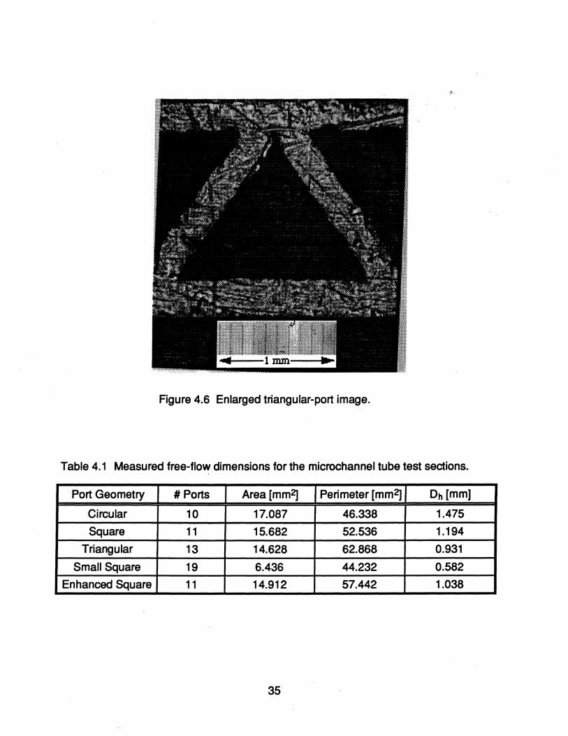
variability presented considerable difficulty. Figure 4.6 is the enlarged image of a

triangular port, which serves as an example (images of the other geometries are

contained in Appendix A). Measurement of the sides reveals that the triangle is

32

Figure 4.1 Circular-port tube. Figure 4.2 Square-port tube.

Figure 4.3 Triangular-port tube. Figure 4.4 Small square-port tube.

33

~ ...

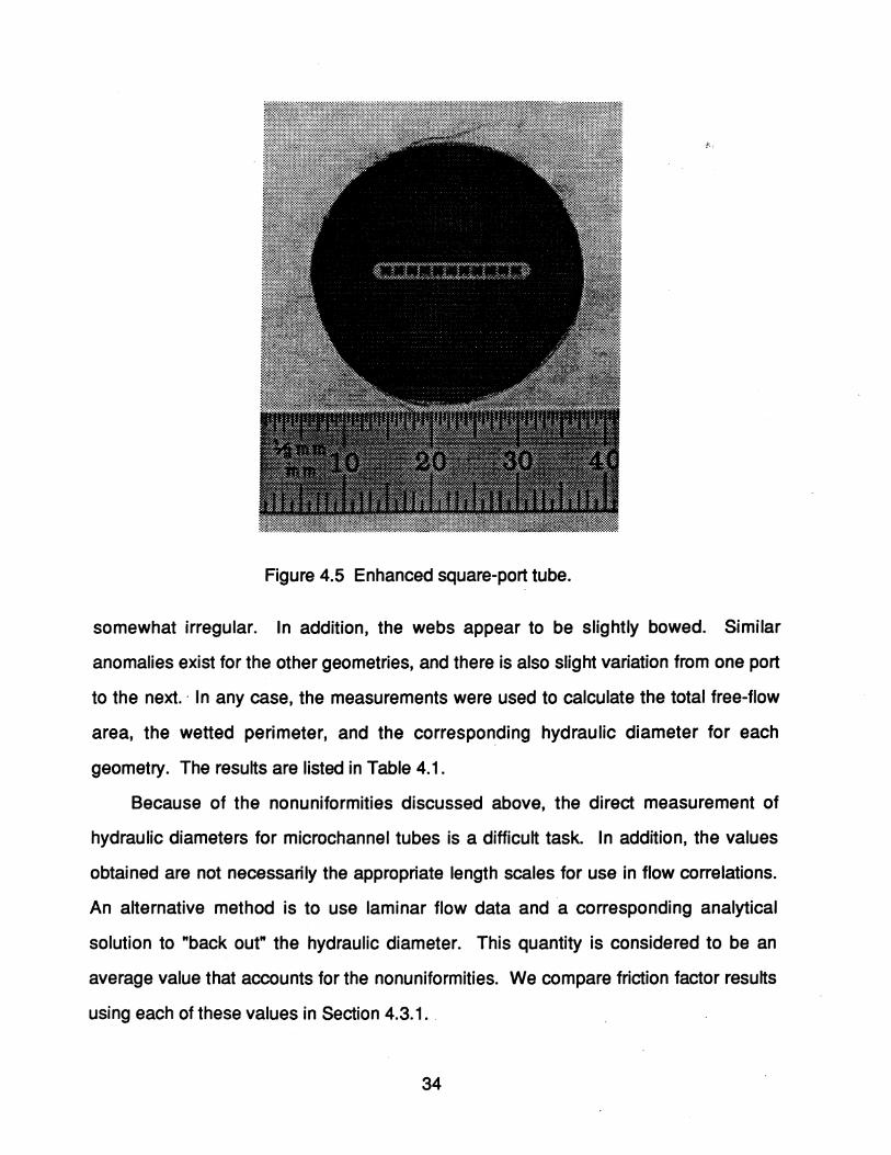
Figure 4.5 Enhanced square-port tube.

somewhat irregular. In addition, the webs appear to be slightly bowed. Similar

anomalies exist for the other geometries, and there is also slight variation from one port

to the next.· In any case, the measurements were used to calculate the total free-flow

area, the wetted perimeter, and the corresponding hydraulic diameter for each

geometry. The results are listed in Table 4.1.

Because of the nonuniformities discussed above, the direct measurement of

hydraulic diameters for microchannel tubes is a difficult task. In addition, the values

obtained are not necessarily the appropriate length scales for use in flow correlations.

An alternative method is to use laminar flow data and a corresponding analytical

solution to "back out" the hydraulic diameter. This quantity is considered to be an

average value that accounts for the nonuniformities. We compare friction factor results

using each of these values in Section 4.3.1.

34

~"

Figure 4.6 Enlarged triangular-port image.

Table 4.1 Measured free-flow dimensions for the microchannel tube test sections.

Port Geometry # Ports Area [mm2] Perimeter [mm2] Dh [mm]

Circular 10 17.087 46.338 1.475

Square 11 15.682 52.536 1.194

Triangular 13 14.628 62.868 0.931

Small Square 19 6.436 44.232 0.582

Enhanced Square 11 14.912 57.442 1.038

35

4.1.2 Nitrogen Test Facility Data Collection

~ .. The Nitrogen Test Facility (NTF) is used to gather data with the intention of

determining friction factors for fully developed flow in microchannel tubes. However, the

measured pressure drop across a test section includes contributions associated with the

entrance region. In particular, these contributions are due to: (a) the cross-sectional

area change from the pressure tap in the transition section to the inlet of the test

section, (b) the sharp entrance of the test section, and (c) the changing momentum flux

and the increased friction in the hydrodynamic development length.

Because these entrance effects are difficult to quantify analytically, we use an

experimental approach to handle ~hem in a conglomerate fashion. An obvious solution

is to take measurements along the entire tube length to obtain a pressure drop in the

fully developed region. However, we are unable to do so because of the microchannel

tube geometry. Instead, we test different lengths of tube at a given flow rate and

assume that the additional pressure drop is due to fully developed flow in the added

length. This method requires that the test sections be identical in every regard except

for the length of the tube. For this reason, the test sections for each type of

microchannel geometry were cut from the same extrusion roll using the same cutting

technique.

For a given microchannel tube geometry, we record flow data using a 12 in. test

section. The data include the atmospheric pressure, the inlet pressure, and the inlet

temperature for a set of mass flow rates. In accordance with the procedure described

above, we record these values for the same set of mass flow rates using 18 in., 25 in.,

30 in., and 36 in. test sections.

All of the values are entered into a data collection log. UHimately, the data are

reduced to obtain-friction factors in the laminar, transition, and turbulent flow regimes.

36

4.1.3 R134a Test Facility Data Collection

;r ..

The R134a Test Facility (RTF) is used to gather heat transfer data for single-phase

flow in microchannel tubes. For these tests, aluminum louvered fins are brazed to the

outside of the tubes to reduce the air-side thermal resistance (see Figure 1.1). The

increased heat transfer leads to more accurate measurements.

We use test section lengths of 25 in. for each microchannel tube geometry. The

test section under consideration is carefully installed and leak-tested before taking data

Because the inlet transition section is identical to that of the NTF, we rely on the

nitrogen data to characterize the hydrodynamic entrance effects.

The data collection procedure consists of setting the desired flow conditions and

recording the data using a Fluke™ data acquisition system. The flow conditions are

maintained by process controllers monitoring the output of test facility components. For

a given microchannel tube test section, we record pressures and temperatures for a set

of refrigerant mass flow rates. We also record the inlet temperature, outlet temperature,

and mass flow rate for the cross-flow air. However, the inlet temperature and mass flow

rate of the air are held constant in order to maintain a constant thermal resistance. The

need for an unchanging air-side resi.stance is discussed in Section 4.2.4.

The refrigerant-side heat transfer rate and the air-side heat transfer rate are easily

calculated from the measurements above. For a properly insulated arrangement, one

expects these values to be equal. Heun (1995) shows that the RTF achieves an energy

balance within 3%, which indicates the integrity of the measurements.

Data in the Reynolds number range of 1000-7000 are obtained for the flow of

subcooled liquid through the test section. Also, the flow of superheated vapor leads to

measurements in the Reynolds number range of 10000-70000. The data in these

ranges are analyzed to yield refrigerant-side Nusselt numbers. However, data outside

of these ranges are not attainable using the RTF.

37

4.2 Data Reduction ~ .. -

4.2.1 Nitrogen Test Facility Entrance Coefficients

As discussed in Section 4.1.2, we test several tube lengths in the Nitrogen Test

Facility to determine the contribution of entrance effects to the overall pressure drop.

Analysis of the data is based on a slightly modified version of Equation 2.3:

(4.1 )

where fo is the fully developed Darcy friction factor and KNTF is a ·coefficient

representing the entrance effects. The subscript "NTP indicates that KNTF includes the

effects due to the transition section in addition to those associated with the

hydrodynamic development length. Accordingly, KNTF is a conglomerate value that

should not be confused with the pressure drop number K-.

Referring to Equation 4.1, KNTF is the nondimensional pressure drop for a tube

length approaching zero. Therefore, we determine the value of KNTF at a given mass

flow rate by (a) plotting the left hand side of Equation 4.1 versus the tube length and (b)

extrapolating a curve fit to find the y-intercept. For each case, the value of p is based

on the inlet properties and V is calculated from the continuity expression

til = pVA (4.2)

where til is the mass flow rate and A is the free-flow area found in Table 4.1. For the

case of incompressible flow, one expects the curve to be linear.

38

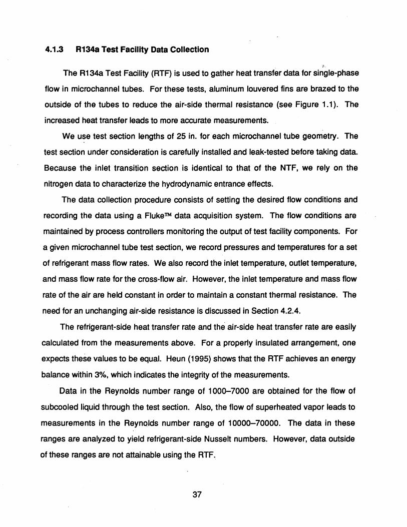
Figure 4.7 shows the results of this procedure for the circular-port tubes.

Although data were taken for many flow rates, only three cases are shown for the sake

of clarity. The data corresponding to Re = 570 are highly linear, which is not surprising

because one expeds the flow to be incompressible for this case. However, the data for

Re = 16250 also exhibit a high degree of linearity, which suggests that compressibility

effeds are not very substantial. For each case, the curve through the data is a least­

squares fit, and the corresponding y-intercept is the value of KNTF. The data associated

with the other flow rates are also found to be linear.

Figure 4.8 displays the corresponding values of KNTF. Although the values appear

to be somewhat random, there are several noticeable features. First, KNTF begins to

decrease sharply at Re = 2100, which marks the transition from laminar to turbulent

. flow. We exped this behavior because the entrance effeds associated with the

hydrodynamic development length are charaderistically smaller for the turbulent case.

100

-- 80

---C\I

60 > 0-Le) .

40 0 ""-a. <::J 20

0 0 20 40 60 80 100

L [em]

Figure 4.7 Dimensionless pressure drop versus length for the circular-port tubes.

39

5 *"

4 0

0 - 0

I 3 ooooo/:, -- o 0

0::'

0

u. 0

Jz :,,'a 0

2 0 ~

o 0 0

1

0 1000 10000

Re [ -]

Figure 4.8 NTF entrance coefficients for the circular-port test section.

There is a second peak in the range of 3000 < Re < 4000, but we cannot offer an

explanation due to the nature of the transition regime. Finally, the values increase

monotonically for Re > 10000 because the contribution associated with the NTF

transition section begins to dominate.

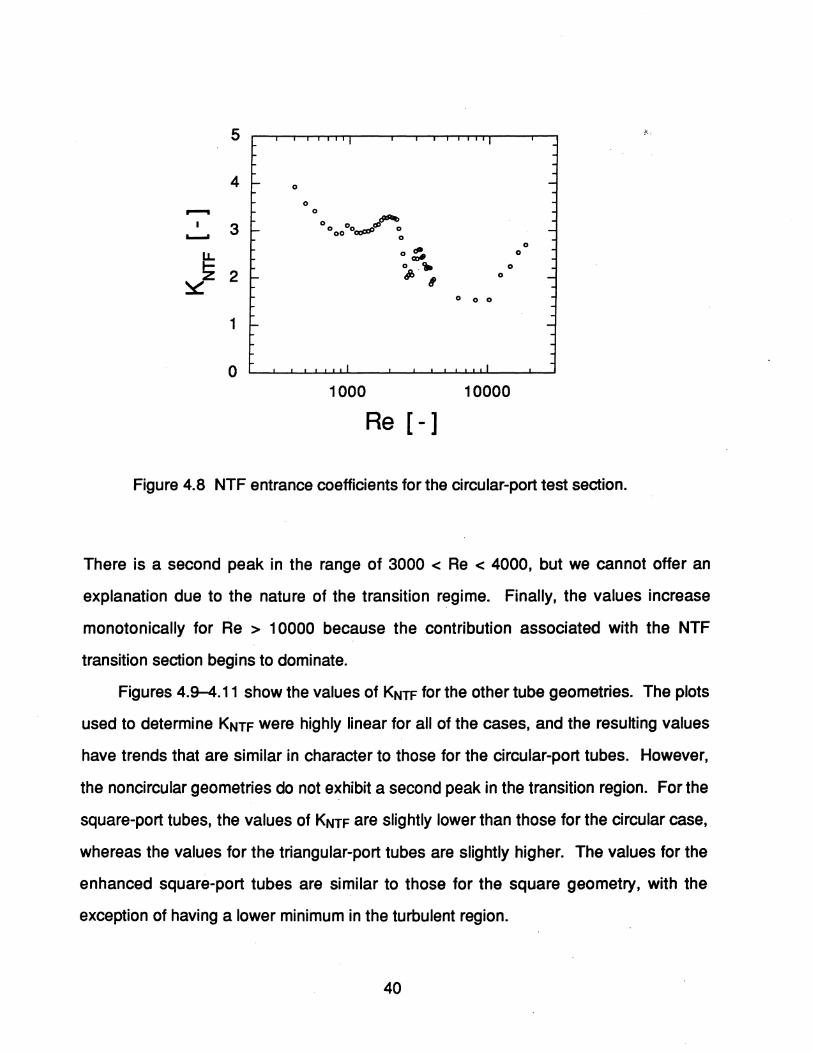
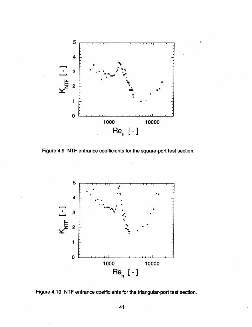
Figures 4.9-4.11 show the values of KNTF for the other tube geometries. The plots

used to determine KNTF were highly linear for all of the cases, and the resulting values

have trends that are similar in character to those for the circular-port tubes. However,

the noncircular geometries do not exhibit a second peak in the transition region. For the

square-port tubes, the values of KNTF are slightly lower than those for the circular case,

whereas the values for the triangular-port tubes are slightly higher. The values for the

enhanced square-port tubes are similar to those for the square geometry, with the

exception of having a lower minimum in the turbulent region.

40

5 *';

4 'b

D D - aD III a

3 D

D D D rI' D D

~ GaDa,.,- .a a

t= a a

liiio a

2 '" ~ a .. DD

a a a

1 a a

0 1000 10000

Reh [ - ]

Figure 4.9 NTF entrance coefficients for the square-port test section.

5 &&

& &

& & & &&

& &

4 & & & &

& & & - ......... : &

I 3 a., &

1*& & ~

& &

t= &

.... & &

~ 2 &

""-- &

&

1

0 1000 10000

Reh [-]

Figure 4.10 NTF entrance coefficients for the triangular-port test section.

41

5 ~: .-

I I

4 r- -

...--. • • • 3 - -...... ".. .. --- • • • •

'" LL •• ..-2

... -£ r- • -..

• • ....

1 . ,

• - • • -

•

0 I I

1000 10000

Reh [ - ]

Figure 4.11 NTF entrance coefficients for the enhanced square-port test section.

4.2.2 Flow Analysis for Friction Factors and UA Values

In this section, we establish the governing equations for single-phase flow through

the microchannel tubes. Figure 4.12 illustrates a differential test section length having

an arbitrary set of inlet conditions. For the case of nitrogen flow through the test

section, the outside of the tube is thermally insulated. In contrast, louvered fins are

attached to the tube when collecting R134a heat transfer data. We apply conservation

equations to relate the differential change in the flow conditions to the friction factor and

the overall thermal conductance UA. Ultimately, these equations are integrated over the

length of the tube to determine average friction factors and UA values corresponding to

experimentally measured inlet and exit conditions.

42

p + dp, p + dp, T + dT, V + dV

x +dx

p, p, T, V x

Figure 4.12 Differential section of a microchannel tube.

CpnseNaUonofMass

We begin by applying the steady-state conservation of mass expression to the

control volume of Figure 4.12:

(4.3)

yielding

(p+dp)(V +dV)A-pVA = 0 (4.4)

and

d(pVA) = 0 (4.5)

and finally

ri1 = pVA = constant (4.6)

where ri1 is the mass flow rate and A is the free-flow area. The fluid velocity V is the

average value at a particular cross section. In the development of Equation 4.6, we

assume that the density variation over the cross-sectional area is negligible. However,

we do consider the possibility of density variation along the axis of the tube.

43

Conservation of Momentum

Next, we apply the conservation of momentum expression:

(4.7)

yielding

PA-(P+ dp dX)A-twP dx = [J3ri1V +~(J3ri1V)dX]-J3ri1V (4.8) dx . dx

where tw is the average wall shear stress and P is the wetted perimeter. The

momentum-flux correction factor J3 accounts for the variation of u2 over the cross section

and is given by

(4.9)

where u is the local value of the velocity. For most cases, the momentum-flux

correction has a negligible effect because values of J3 are close to 1.0. Equation 4.8 is

simplified further to obtain

d (J3ri1V ) P - --+p +t -=0 . dx A w A

(4.10)

At this point, we substitute Equation 2.1 along with the definition of the hydraulic

diameter

4A Dh =--=-p (4.11 )

to obtain

44

d (fJrilV ) pV2 - --+p =--/0 dx A 2Dh

;>, (4.12)

where fo is the local value of the Darcy friction factor. Equation 4.12 reduces to

Equation 2.2 for the case of incompressible flow in the fully developed region.

Conservation of EneCQ'y

Referring to Figure 4.12, we define a quantity q as the rate of heat transfer

between the fluid and the surroundings for a length of tube extending from the inlet to a

location x. With this definition of q, the conservation of energy expression is given by

(4.13)

so

and

d [ . (.. V2 J] dq dx m h+a2 = dx (4.15)

where Ii is the fluid enthalpy. The kinetic-energy correction factor a accounts for the

variation of u3 over the cross section and is given by

1 (U)3 a= AJJA V dA (4.16)

where u is the local value of the velocity. The kinetic-energy correction usually has a

negligible effect because values of a are close to 1.0.

45

Referring to Equation 4.15, the value of q is zero for the nitrogen flow tests

because the tube is thermally insulated. For the refrigerant flow tests, there is a cross­

flow heat exchanger arrangement with air as the external fluid. We define the following

heat capacity rates:

Cref = rT1refCp,ref

Cair = rT1airCp,air }

Cmin = min( Cref , Cair )

Cmax = max(Cref,Cair)

where Cp is the specific heat, and the subscript "rer refers to the R134a refrigerant. The

corresponding value of q is given by

dq de ( ) -=-C· T· ·-T . dx dx min alr,l ref,l (4.17)

where e is the heat exchanger effectiveness from the inlet of the tube to an arbitrary

location x, and the subscript "i" refers to the inlet value. The analysis of Mason (1954)

leads to the following expression for our heat exchanger arrangement:

where 8 and ~ are dummy variables of integration. Due to the complexity of this

expression, the differentiation of e in Equation 4.17 must be handled numerically.

Thermodynamic Relations

In addition to the conservation equations, we have the following thermodynamic

relations:

46

p = p(p,T)

h = h(p, T) .

4.2.3 Integration of the Conservation Equations

1'-.

(4.19)

(4.20)

The conservation equations presented in Section 4.2.2 are used to determine

friction factors and UA values from the experimental data. The equations are cast into a

convenient form for integration by defining

and

lirilV Z1=--+P

A (4.21 )

(4.22)

After substituting these definitions into the momentum and energy equations (4.12 &

4.15), we make use of the mass conservation equation (4.6) and the thermodynamic

relations (4.19 & 4.20) to obtain

Ii (ril)2 Z1 = p(p,T) A +p, (4.23)

(4.24)

dZ1 1 (ril)2 fo dx = - pep, T) A 2Dh '

(4.25)

and

dZ2 = dq = f(x,UA) dx dx

(4.26)

47

As mentioned previously, the value of q is zero for the nitrogen flow tests.

Consequently, the fundion f is also zero for this case. For the refrigerant flow tests, the

fundion f is given by Equation 4.17.

Equations 4.25 and 4.26, in conjundion with the definitions of Z1 and Z2, constitute

a pair of coupled ordinary differential equations. The boundary conditions are the inlet

pressure and the inlet temperature, and the mass flow rate is also known from the data.

We determine values of to and UA such that the integration of these equations along

the tube length produces the measured values of the pressure and temperature at the

exit. Accordingly, to and UA are considered to be integrated-average values.

We determine values of p(p,T) and h(p,T) for the nitrogen and the R134a using

fluid property subroutines. As a consequence, the integration of Equations 4.25 and

4.26 must be done numerically. Specifically, we employ the following algorithm for the

determination of to and UA:

(1) Guess the values of to and UA.

(2) Determine the values of Z1 and Z2 at x=O from the inlet values of the pressure and

temperature (using Equations 4.23 and 4.24).

(3) Integrate Equations 4.25 and 4.26 numerically to determine the values of Z1 and Z2

at each x. In particular, we use a marching routine that requires evaluation" of the

right hand sides of Equations 4.25 and 4.26 at deSignated values of x. The values

of p and T required to evaluate the RHS of Equation 4.25 are found by solving

Equations 4.23 and 4.24 simultaneously using the values of Z1 and Z2 at that x.

(4) Determine exit values of p and T from the values of Z1 and Z2 at x=L (by solving

Equations 4.23 and 4.24 simultaneously).

(5) Compare the values of p and T from step (4) to the measured values. If the values

are equal, then stop. Otherwise, adjust the values of to and UA and go to step (2).

48

A FORTRAN computer program executes the steps above. The numerical integration

of step (3) is performed by the well known "ode" subroutine given by Shampine and

Gordon (1975), and the simultaneous solution of Equations 4.23 and 4.24 is performed

by a robust Newton-Raphson subroutine given by Press et al. (1992). With regard to

step (5), the program actually conducts a two-dimensional search for to and UA within

bounds provided for each of these values. We assume that the values found in this

manner are a unique combination. Once the values of to and UA are found, the

program calculates the Reynolds number at each x location and determines a

corresponding average value.

The procedure above is simplified for the nitrogen tests because the UA value is

known to be zero. Accordingly, we use a modified version of the program which

searches for the to that yields the measured exit pressure. This version of the program

is contained in Appendix B.

As discussed in Section 4.2.1, the NTF entrance coefficient KNTF is the

nondimensional pressure drop due to entrance effects. These coefficients also apply to

the RTF flows because the transition section at the inlet is identical to that of the NTF.

For each Reynolds number, the value of KNTF is used to subtract the pressure drop due

to entrance effects from the measured inlet pressure. The resulting value is used as the

pressure at x=O. As a consequence, the fully developed value of to·is found from the

program.

With regard to the temperature at x=O, we assume that the value is i~entical to the

measured value (i.e., we neglect any temperature change from the tap in the transition

section to the inlet of the tube). For the refrigerant flow tests, we account for the thermal

development length by (a) determining the average Nusselt number from the UA value

(as discussed in Section 4.2.4) and (b) using Equation 2.28 to estimate the fully

developed Nusselt number.

49

By using the program to integrate the conservation equations, we account for the

effects of compressibility (for the high-Re flows) and property variation. We assume that

the integrated-average values of /0 and Nu that result from this analysis can be

compared to the values obtained from the incompressible flow correlations of Chapter 2.

4.2.4 Wilson Plot Analysis for Nusselt Numbers

After determining UA values from the RTF data, a Wilson plot (Stoecker & Jones

(1982)) is used to determine the amount of thermal resistance due to the tube wall and

the air flow. This amount is subtracted from the total thermal resistance to obtain the

refrigerant-side resistance at a particular refrigerant flow rate. Finally, the refrigerant­

side resistance is used to calculate the Nusselt number.

The Wilson plot is based on the following equation for the total thermal resistance:

1 Rtot = UA = Rref + Rwalt + Rair (4.27)

where the subscript "wall" refers to the outer wall of the microchannel tube plus the

attached fins (see Figure 1.1). For a particular test section, the value of Rwall is

assumed to be constant (Le., we neglect the variation of the thermal conductivity with

temperature). The value of Rair is also assumed to be constant because the mass flow

rate of the air is held constant for each data set. Consequently, we expect the plot of

Rtot versus Rref to be a straight line with (Rwalt + Rair ) as the y-intercept.

When constructing the Wilson plot, the values of Rtot are known from the data.

However, the values of Rref are initially unknown and .must be. modeled. For flow in a

microchannel tube, the refrigerant-side resistance is given by

Rref =- ( ) href 1'\fSf,ref + Sp,ref

1 . (4.28)

50

where hAl' is the average heat transfer coefficient of the refrigerant. Referring to Figure

4.12, the webs of the individual ports act as fins with an efficiency Tlf. The wetted

surface area for heat transfer consists of (a) the fin area St,ref, which is the surface area

of the webs in contact with the refrigerant, and (b) primary area Sp,ref, which is the

surface area of the tube wall in contact with the refrigerant. The fin efficiency Tlf is .

determined from a one-dimensional fin analysis, and the average heat transfer

coefficient hAl' is calculated from Equation 2.22 (Gnielinski (1976».

For each set of refrigerant flow rates, we plot the values of Rtot versus the

predicted values of Rref. A least squares straight line is fitted through the data, and a

straight line extrapolation is made to find the y-intercept (Rwall + Rair). If the model for

Rref is correct, then the slope of the line is equal to unity. Even if the model is off by a

constant factor, the correct value of (Rwall + Rair) is obtained provided Equation 2.22

accurately reflects the functional dependence of hre, on Re and Pro In this case, the

slope of the straight line is a value other than unity. Once the value of (Rwall + Rair) is

found, Equation 4.27 is used to determine the actual value of Rref for each refrigerant

flow rate. Finally, Equation 4.28 is used to determine the values of hre' and ultimately

the Nusselt numbers.

Figure 4.13 shows the V"ilson. plot for superheated re~rigerant flow through the

circular-port test section. Data corresponding to three different air flow rates are shown

for the sake of comparison. As expected, the y-intercept (Rwall + Rair) decreases with

increasing air flow rate. For each case, the data exhibit a high degree of linearity,

indicating that Equation 2.22 accurately predicts the dependence of hAl' on Re and Pro

The slopes of the lines, from the lowest air flow rate to the highest, are 0.91, 0.92, and

0.95. The fact that these slopes are close to unity indicates that the model used for Rref

is fairly accurate for superheated refrigerant flow through the circular-port test section.

51

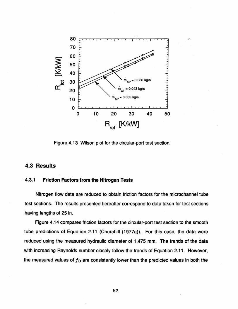
80 1'"

70

~ 60

50

52 40 ~

'0 30 ,nair - 0.030 kg/s

a:.-20 ,nair - 0.043 kg/s

10 ,nair - 0.055 kg/s

0 0 10 20 30 40 50

R ref

[K/kW]

Figure 4.13 Wilson plot for the circular-port test section.

4.3 Results

4.3.1 Friction Factors from the Nitrogen Tests

·Nitrogen flow data are reduced to obtain friction factors for the microchannel tube

test sections. The results presented hereafter correspond to data taken for test sections

having lengths of 25 in.

Figure 4.14 compares friction factors for the circular-port test section to the smooth

tube predictions of Equation 2.11 (Churchill (1977a)). For this case, the data were

reduced using the measured hydraulic diameter of 1.475 .mm. The trends of the data

with increasing Reynolds number closely follow the trends of Equation 2.11. However,

the measured vafues of fo are consistently lower than the predicted values in both the

52

0.1

--

0.01 1000

-- Equation 2.11 for smooth circular ducts

o

10000

Re [-]

Figure 4.14 Circular-port results using the measured hydraulic diameter.

laminar and turbulent regimes.

1-•.

In the laminar regime, Equation 2.11 reduces to the laminar flow solution given by

Equation 2.4. Because the laminar flow solution is well established, we suspect that the

deviation in this regime is due to the inaccuracy of the measured hydraulic diameter

(see Section 4.1.1). Better results are obtained by using Equation 2.4 in conjunction

with the laminar flow data to calculate a value for the hydraulic diameter. In particular,

we substitute Equation 2.4 into the momentum equation (4.25) so that the hydraulic

diameter becomes the unknown quantity in the data reduction procedure. Referring to

Equations 4.23-4.25, the free-flow area A is written in terms of the hydraulic diameter

as follows:

(4.29)

53

where Np is the number of ports (listed in Table 4.1) and Deq is the equivalent diameter

of a port as defined by Equation 4.29. The nondimensional equivalent diam~ter D~ is

equal to 1.0 for the circular ports. For the square and triangular ports, the value of D~

is a constant depending only on the shape. After substituting Equation 4.29 for the free­

flow area A, we solve Equations 4.23-4.26 to determine a value for the hydraulic

diameter corresponding to each laminar data point. The arithmetic average of these

values is considered to be the appropriate Dh. Finally, we use this value of Dh to reduce

the set of friction factor data.

Referring to Figure 4.14, similar deviations from the laminar flow solutions occur for

the other test section geometries. Consequently, we use the procedure described

above to calculate values of Dh for the square, triangular, and small square geometries.

However, a value for Dh cannot be calculated for the enhanced square geometry

because the friction constant Kf in Equation 2.4 is unknown for this case. Therefore, we

rely on the measured Dh in order to calculate the value of Kf using the same procedure.

Table 4.2 lists the values of Kf and D:q for each geometry, along with the

associated value of Dh. In all cases, the values of Dh calculated from the laminar data

are slightly larger than the measured values listed in Table 4.1. Also included in Table

4.2 are the length scales Ole and Die discussed in Section 2.2.2.

Table 4.2 Geometric parameters for the microchannel tube test sections.

Port Geometry Kf [-] D;q [ - ] Dh [mm] Ole [mm] Die [mm]

Circular 64.000 1.000 1.494 1.494 1.494

Square 56.908 1.128 1.214 1.366 1.465

Triangular 53.332 1.286 0.944 1.133 1.416

Small Square· 56.908 1.128 0.619 0.696 0.747

Enhanced Square 57.800 1.265 1.038 1.149 n/a

54

Figure 4.15 shows the friction factors obtained for the circular-port test section

using the calculated Dh of 1.494 mm.· Although this value is only 1.3% larger than the

measured hydraulic diameter, the agreement with Equation 2.11 is significantly

improved. in the turbulent regime (we expect agreement in the laminar regime, of

course, because the laminar flow solution itself was used to calculate Dh). Evidently,

the values obtained for the friction factor are quite sensitive to the value used for the

hydraulic diameter. All of the results presented hereafter are based on the calculated

hydraulic diameters from Table 4.2.

Referring to Figure 4.15, the critical Reynolds number is found to be 2100 for the

circular-port test section. This number is in excellent agreement with the value of 2115

reported by Obot (1988) for smooth circular ducts. Equation 2.11 (Churchill (19na))

accurately predicts the friction factors in the laminar, transition, and turbulent regimes.

Interestingly, there does not appear to be any rough-tube behavior or small length scale

0.1

0.01 1000

--Equation 2.11 for smooth circular ducts

10000

Re [-]

Figure 4.15 Friction factors for the circular-port test section.

55

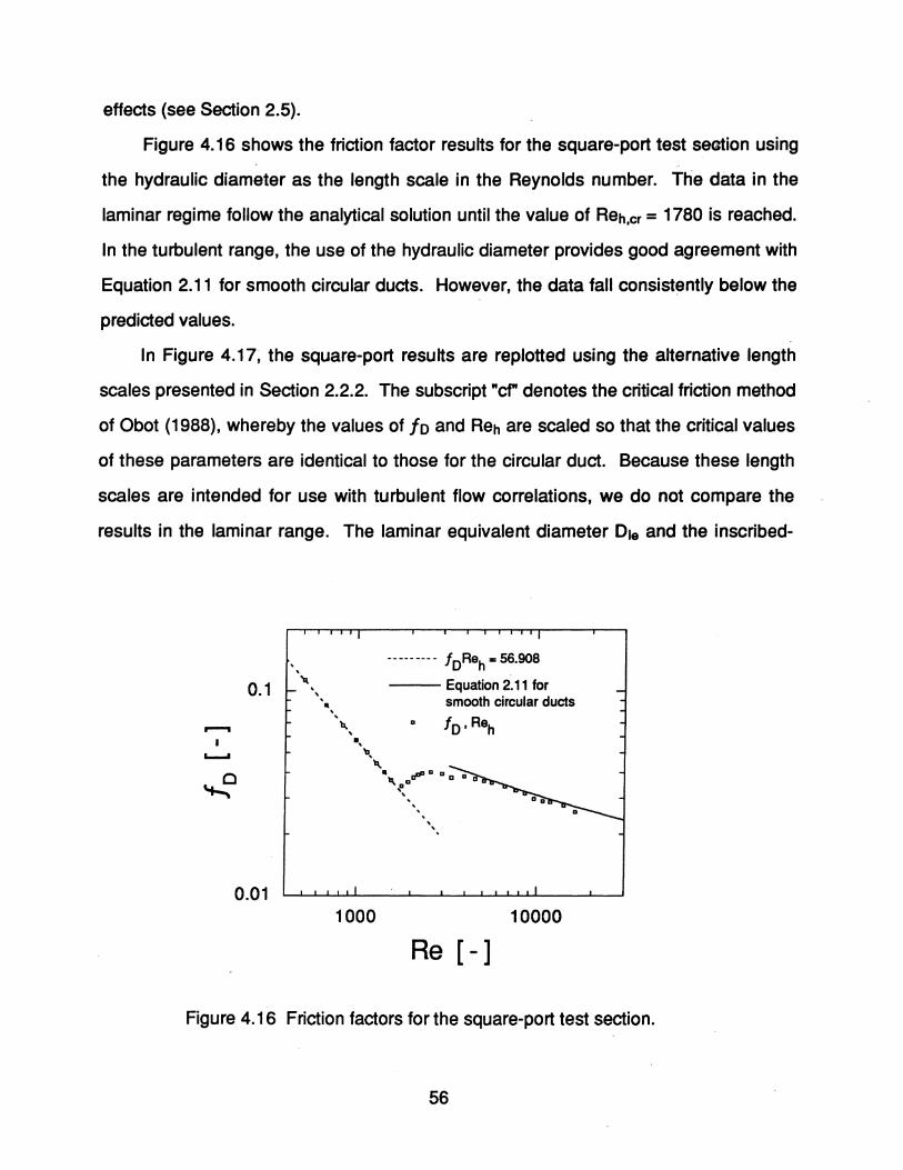
effects (see Section 2.5).

Figure 4.16 shows the friction factor results for the square-port test semion using

the hydraulic diameter as the length scale in the Reynolds number. The data in the

laminar regime follow the analytical solution until the value of Reh,cr = 1780 is reached.

In the turbulent range, the use of the hydraulic diameter provides good agreement with

Equation 2.11 for smooth circular ducts. However, the data fall consistently below the

predicted values.

In Figure 4.17, the square-port results are replotted using the alternative length

scales presented in Section 2.2.2. The subscript "ef" denotes the critical friction method

of Obot (1988), whereby the values of fo and Reh are scaled so that the critical values

of these parameters are identical to those for the circular duct. Because these length

scales are intended for use with turbulent flow correlations, we do not compare the

results in the laminar range. The laminar equivalent diameter Ole and the inscribed-

,

0.1 '",

--

0.01 1000

--------- toReh - 56.908

-- Equation 2.11 for smooth circular ducts

a to' Reh

, "

10000

Re [-]

Figure 4.16 Friction factors for the square-port test section.

56

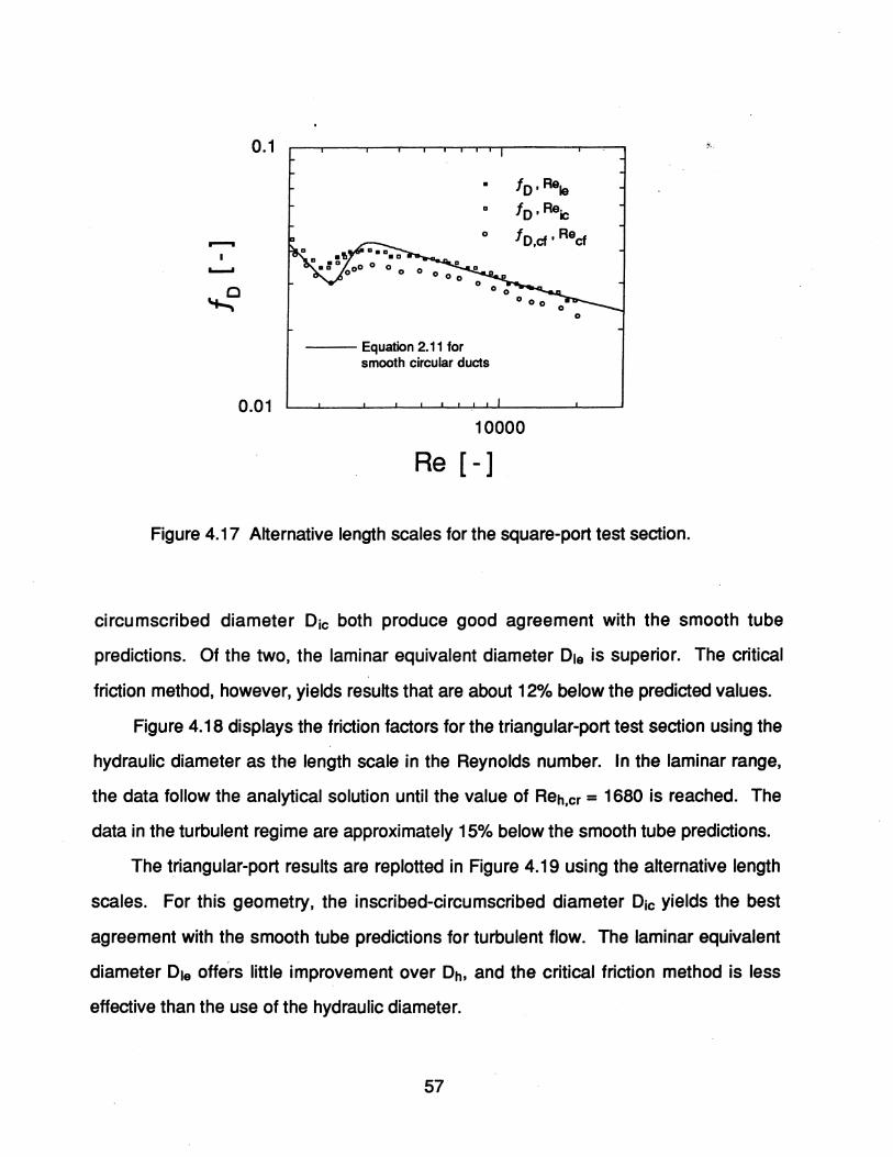
0.1

0.01

• D

o

--Equation 2.11 for smooth circular ducts

'0 I Rele

'0 I Reic

'O,ef I Reef

o

10000

Re [-]

Figure 4.17 Alternative length scales for the square-port test section.

circumscribed diameter Dic both produce good agreement with the smooth tube

predictions. Of the two, the laminar equivalent diameter Ole is superior. The critical

friction method, however, yields results that are about 12% below the predicted values.

Figure 4.18 displays the friction factors for the triangular-port test section using the

hydraulic diameter as the length scale in the Reynolds number. In the laminar range,

the data follow the analytical solution until the value of Reh,cr = 1680 is reached. The

data in the turbulent regime are approximately 15% below the smooth tube predictions.

The triangular-port results are replotted in Figure 4.19 using the alternative length

scales. For this geometry, the inscribed-circumscribed diameter Dic yields the best

agreement with the smooth tube predictions for turbulent flow. The laminar equivalent

diameter Ole offers little improvement over Dh, and the critical friction method is less

effective than the use of the hydraulic diameter.

57

....... I .........

0.1

0.01

--------- toRah" 53.332

--- Equation 2.11 for smooth circular ducts

IJ. to ' Rah

'A,.

~ 'It »6 t. t.t. t. t. t.t. t.

" ,

1000

, , , ,

Re [-] 10000

Figure 4.18 Friction factors for the triangular-port test section.

0.1

.........

0.01

--- Equation 2.11 for smooth circular ducts

10000

Re [-]

Figure 4.19 Alternative length scales for the triangular-port test section.

58

Figure 4.20 displays the friction factors for the small square-port test section using

Reynolds numbers based on the hydraulic diameter. The data in the laminar regime

follow the analytical solution until reaching the value of Reh,cr = 2000, which is 12%

higher than the critical Reynolds number of the larger square-port test section. In the

turbulent range, the data for Reh > 5000 approach the smooth tube predictions and

appear to be similar in character to the data for the larger square-port test section.

In Figure 4.21, the small square-port results are replotted using Reynolds numbers

based on the alternative length scales. For this test section. the laminar equivalent

diameter, the inscribed-circumscribed diameter, and the critical friction method all

produce good agreement with Equation 2.11 for Re > 6000. However, the results using

the alternative length scales are only slightly different than those corresponding to the

hydraulic diameter (see Figure 4.20).

• " 0.1 ",

"

.--. I --

0.01

--, , • ,

'q , , ,

1000

-, ,

--------- foReh -56.908

--Equation 2.11 for

a

'II a '.pa , ,

smooth circular ducts

fO,Rsh

10000

Re [-]

Figure 4.20 Friction factors for the small square-port test section.

59

0.1 ;s'.

• 10 , Reje

a 10 , Reic

0 IO,ef' Reef --.........

~ Equation 2.11 for smooth circular ducts

0.01 10000

Re [ - ]

Figure 4.21 Alternative length scales for the small square-port test section.

Figure 4.22 shows the friction factors for the enhanced square-port test section

using Reynolds numbers based on the hydraulic diameter. The data in the laminar

range follow the analytical solution until reaching the value of Reh,cr = 1770. In the

turbulent range, the use of the hydraulic diameter provides good agreement with the

predictions of Equation 2.11.

The enhanced square-port results are replotted in Figure 4.23 using the laminar

equivalent diameter Ole and the critical friction method. The use of Ole produces good

agreement with Equation 2.11 for Rele > 5000. However, the critical friction method

yields results that are about 20% below the predicted values.

As indicated by Figures 4.15-4.23, the values of Reh,cr for the noncircular test

sections are all smaller than the value of 2100 for the circular test section. In addition,

60

-........

c . '+-..

0.1

0.01

"

1000

--------- fOReh -57.8

--- Equation 2.11 for

, , ,

• smooth circular ducts

10000

Re [-]

Figure 4.22 Friction factors for the enhanced square-port test section.

0.1

-........

0.01

•

o

--- Equation 2.11 for smooth circular ducts

10000

Re [-]

Figure 4.23 Alternative length scales for the enhanced square-port test section.

61

the trends of the data in the transition region are flatter for the noncircular test sections.

The data in the turbulent region, however, follow Equation 2.11 for smooth circular tubes

provided that the appropriate length scale is used in the Reynolds number. Thus, the

tubes do not exhibit any roughness or small length scale effects.

4.3.2 Nusselt Numbers from the R134a Tests

R134a flow data are reduced to obtain Nusselt numbers for the microchannel tube

test sections. In the results that follow, data for 1000 < Re < 7000 correspond to the

flow of subcooled liquid having a Prandtl number of 3.55. Similarly, data for 10000 < Re

< 70000 correspond to the flow of superheated vapor having a Prandtl number of 0.84.

Figures 4.24-4.28 compare the Nusselt numbers for the microchannel tube test

sections to the predictions of Equation 2.22 (Gnielinski (1977)) and Equation 2.24

(Churchill (1977b}). For each tube geometry, we use a characteristic length that

produces agreement between the experimental friction factors and the circular tube

predictions (see Section 4.3.1). With the exception of the small square-port data, all of

the experimental Nusselt numbers are larger than the predicted values. For Reynolds

numbers less than 10000 (subcooled-liquid data), most of the experimental values are

in better agreement with Equation 2.24. In contrast, the experimental values are in

better agreement with Equation 2.22 for Reynolds numbers greater than 10000

(superheated-vapor data). The character of the superheated-vapor data is very

conSistent, and the values are within 10% of Equation 2.22. The character of the

subcooled-liquid data is less consistent, however, and some values differ significantly

from the predictions. At this point, it is unclear as to whether the deviation is due to a

Reynolds number effect or a Prandtl number effect.

62

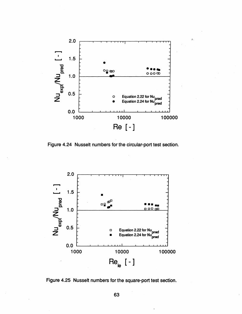
2.0 ~ .. I

r-""'I

....... 1.5 f- --"C e o~ ClIX) ---. a. 00000 ::l 1.0 -Z "'"-c.

x CD 0.5 ::l - Equation 2.22 for NUpred

-Z

0

- Equation 2.24 for NUpred

0.0 I

1000 10000 100000

Ra [ -]

Figure 4.24 Nusselt numbers for the circular-port test section.

2.0 I . r-""'I

....... 1.5 .... -• "C r:JP e a. []~ ... • ••••

::l 1.0 [] [] [] [][]

Z

----a. x CD 0.5 ::l f-

[] Equation 2.22 for NUpred -Z • Equation 2.24 for NUpred

0.0 1

1000 10000 100000

Rale [ - ]

Figure 4.25 Nusselt numbers for the square-port test section.

63

2.0 ~'. I

--- 1.5 - -

~ 66

66. • •••• c.. •••• 66666 :::s 1.0 Z "'--c..

)( CD 0.5 :::s - -

Z 6 Equation 2.22 for Nu ed

• Equation 2.24 for NU~ed

0.0 I

1000 10000 100000

Re. [ - ] Ie

Figure 4.26 Nusselt numbers for the triangular-port test sedion.

3.0 I

-- 2.5 • 0 Equation 2.22 for NUpred · ~ -• Equation 2.24 for NUpred - ·

"C 2.0 - -e • c.. ·

:::s 1.5 - -Z 0 • "a • [J 0

1.0 .., • )( CD

[J

:::s Z 0.5 - ~ ~ ~ ~ ~ -

0.0 I

1000 10000 100000

Rele [ - ]

Figure 4.27 Nusselt numbers for the small square-port test sedion.

64

2.0 I :r ..

- • . .....- 1.5 ~ -

~ .,sP ••••• c.. cc~

::l 1.0 o CCCo

Z

----c.. )( CD 0.5 ::l f-

C Equation 2.22 for NUpred -Z • Equation 2.24 for NUpred

0.0 I

1000 10000 100000

ReJe [ - ]

Figure 4.28 Nusselt numbers for the enhanced square-port test section.

65

5. PROJECT SUMMARY AND CONCLUSIONS

Microchannel heat exchanger technology allows one to design compact air

conditioning condensers with better thermal performance characteristics than standard

condensers. Optimization of the microchannel designs, however, requires an

understanding of the friction and heat transfer phenomena associated with flow in an

individual tube. Therefore, we conducted an experimental investigation of these

phenomena.

As part of a project that includes full condenser modeling and two-phase flow

modeling, data were collected for Single-phase flow in several types of microchannel

tubes. Two test facilities were used for this purpose, including a nitrogen facility for

adiabatic flow data and an R134a facility for heat transfer data. The nitrogen data were

analyzed to obtain friction factors in the Reynolds number range of 500-20000, and the

R134a data were analyzed to obtain Nusselt numbers in the Reynolds number ranges

of 1000-7000 and 10000-70000.

5.1 Summary of Results

For Single-phase flow in the microchannel tubes under consideration, the

experimental data demonstrate the following:

• For each tube geometry, friction factors in the laminar flow regime follow the

analytical solution given by Equation 2.4.

• The critical Reynolds numbers for the noncircular tubes are all smaller than the

value of 2100 for the Circular-port tube.

• For the circular-port tube, friction factors in the transition and turbulent regimes

follow the smooth-tube correlation given by Churchill (1977a).

66

• For the noncircular tubes, friction factors in the turbulent regime follow the Churchill

correlation provided the appropriate length scale is used in the Reynolds number.

The laminar equivalent diameter is appropriate for the square and enhanced

square-port tubes, and the inscribed-circumscribed diameter is appropriate for the

triangular-port tube.

• In light of the statements above, there is no evidence of surface roughness or small

length scale effects.

• For all of the tubes, with the exception of the small square-port type, Nusselt

numbers in the range of 10000-70000 (superheated-vapor data) are within 10% of

the correlation given by Gnielinski (1977).

The Nusselt number data are inconclusive for the small square-port tube. Moreover, the

Nusselt number data are inconclusive for the rest of the tubes in the Reynolds number

range of 1000-7000 (subcooled liquid data).

For each tube geometry, the friction factors obtained in the turbulent regime were

sensitive to the value used for the hydraulic diameter. Use of a hydraulic diameter

calculated from laminar data, as opposed to a value determined from direct

measurement, led to better agreement between measured friction factors and the

predictions of the Churchill correlation.

5.2 Recommendations for Future Research

With regard to single-phase flow in microchannel tubes, we present the following

recommendations for future research:

• Measure friction factors for Reynolds numbers greater than 20000 to determine if

surface roughness becomes important.

67

• Measure friction factors for tubes with decreasing hydraulic diameters to determine if

small length scale effects occur. "

• Conduct a thorough investigation of Nusselt numbers in the Reynolds number range

of 0-10000.

• Investigate the effects of Prandtl number variation for single-phase Nusselt numbers.

68

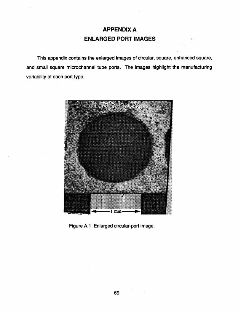
APPENDIX A

ENLARGED PORT IMAGES ~'.

This appendix contains the enlarged images of circular, square, enhanced square,

and small square microchannel tube ports. The images highlight the manufacturing

variability of each port type.

Figure A.1 Enlarged circular-port image.

69

~ .. -

Figure A.2 Enlarged square-port image.

70

Figure A.3 Enlarged small square-port image.

71

:r ..

Figure A.4 Enlarged enhanced square-port image.

72

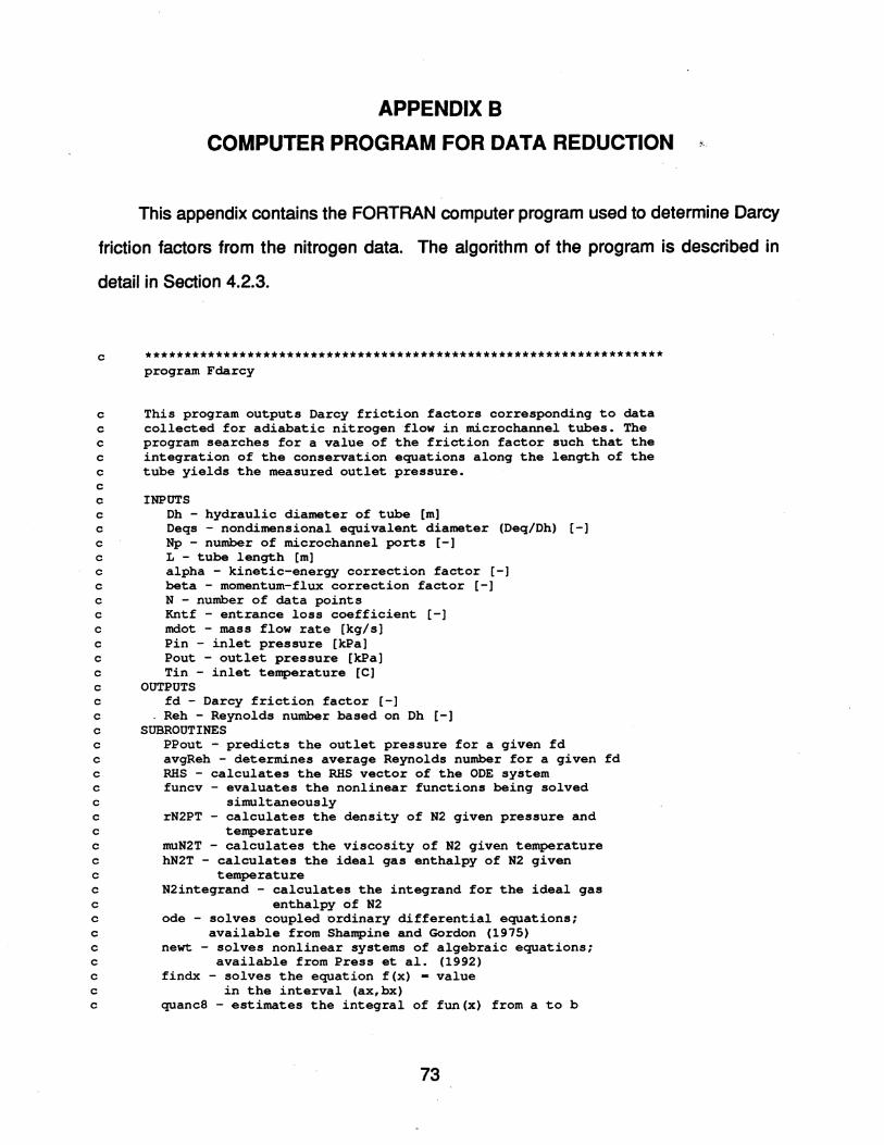
APPENDIX B

COMPUTER PROGRAM FOR DATA REDUCTION '

This appendix contains the FORTRAN computer program used to determine Darcy

friction factors from the nitrogen data. The algorithm of the program is described in

detail in Section 4.2.3.

c ****************************************************************** program Fdarcy

c This program outputs Darcy friction factors corresponding to data c collected for adiabatic nitrogen flow in microchannel tubes. The c program searches for a value of the friction factor such that the c integration of the conservation equations along the length of the c tube yields the measured outlet pressure. c c INPUTS c Dh - hydraulic diameter of tube [m] c Deqs - nondimensional equivalent diameter (Deq/Dh) [-] c Np - number of microchannel ports [-] c L - tube length [m] c alpha - kinetic-energy correction factor [-] c beta - momentum-flux correction factor [-] c N - number of data points c Kntf - entrance loss coefficient [-] c mdot - mass flow rate [kg/s] c Pin - inlet pressure [kPa] c Pout - outlet pressure [kPa] c Tin - inlet temperature [e) c OUTPUTS c fd - Darcy friction factor [-] c . Reh - Reynolds number based on Dh [-] c SUBROUTINES c c c c c c c c c c c c c c c c c c c

PPout - predicts the outlet pressure for a given fd avgReh - determines average Reynolds number for a given fd RHS - calculates the RHS vector of the ODE system funcv - evaluates the nonlinear functions being solved

simultaneously rN2PT - calculates the density of N2 given pressure and

temperature muN2T - calculates the viscosity of N2 given temperature hN2T - calculates the ideal gas enthalpy of N2 given

temperature N2integrand - calculates the integrand for the ideal gas

enthalpy of N2 ode - solves coupled ordinary differential equations;

available from Shampine and Gordon (1975) newt - solves nonlinear systems of algebraic equations;

available from Press et al. (1992) findx - solves the equation f(x) - value

in the interval (ax,bx) quanc8 - estimates the integral of fun (x) from a to b

73

c ...

implicit none character*8 comment integer i, N

double precision Dh, Deqs, Np, L, alpha, beta, & Kntf, mdot, Pin, Pout, Tin

double precision fd, PPout, findx, fdmin, fdmax, & relerr, abserr, Reh, avgReh

parameter (fdmin - O.OdO, fdmax - 0.25dO) parameter (relerr - l.Od-7, abserr - 1.0d-7)

common/inputs/ Dh, Deqs, Np, L, alpha, beta, & Kntf, mdot, Pin, Pout, Tin

external PPout

open (unit open (unit

read input

read (10, *)

10, file 20, file

values

comment

, Fdarcy • in ' ) 'Fdarcy . out' )

read (10, *) Dh, Deqs,Np, L, alpha, beta read (10, *) read (10, *) comment read (10, *) N read (10, *) read (10, *) comment

write (20,*) 'fd, Reh'

do 200 i - 1, N

read (10,*) Kntf,mdot,Pin,Pout,Tin

c... Find friction factor for given Pout fd - findx(PPout, Pout, fdmin, fdmax, relerr, abserr)

c... Find average Reynolds number with known fd Reh - avgReh(fd)

write (20,100) fd, char(9), Reh 100 format (f8.6,a1,f8.1)

200 continue

close (unit 10) close (unit 20)

stop end

c ****************************************************************** function PPout (fd)

implicit none logical check

integer iflag, neqn, wdim, ndiv, i

74

parameter (neqn - 2, wdim - 142, ndiv - 100)

double precision Dh, Deqs, Np, L, alpha, beta, & Kntf, mdot, Pin, Pout, Tin

double precision PPout, fd, tempfd, seg, xO, xin, xout, & relerr, abserr, rler, aber, Pl, P2, T2, & rN2PT, hN2T, kPtoP, CtoK, pi

double precision z(neqn), tempz(neqn), guess(neqn), ptvec(neqn), & work (wdim)

parameter (xO - O.OdO, relerr - 1.Od-7, abserr - 1.Od-7) parameter (kPtoP - lOOO.OdO, CtoK - 273.l5dO) parameter (pi - 3.l4l592654dO)

common/inputs/ Dh, Deqs, Np, L, alpha, beta, & Kntf, mdot, Pin, Pout, Tin

common/fd/ tempfd common/Zvec/ tempz common/Gvec/ guess

external RHS

c This function returns a predicted outlet pressure c PPout [kPa] for a given Darcy friction factor fd [-] c using the 'ode' subroutine.

tempfd - fd

c .•• Find initial values of z(l) and z(2) accounting for c entrance loss

Pl - Pin*kPtoP - Kntf*O.5DO*(4.0dO*mdot/pi/Np/(Deqs*Dh)**2)**2 & /rN2PT ( (Pin*kPtoP) , (Tin+CtoK) )

z(l) - beta*(4.0dO*mdot/pi/Np/(Deqs*Dh)**2)**2 & /rN2PT(Pl, (Tin+CtoK»+Pl

z(2) - mdot*hN2T«Tin+CtoK»+O.5dO*alpha*mdot & * (4.0dO*mdot/pi/Np/(Deqs*Dh)**2)**2 & /(rN2PT(Pl, (Tin+CtoK»)**2

c ••. Call ode routine to integrate governing equations

c. • • grid definition seg - L/dble(ndiv)

c .•• starting conditions ifla9' - 1 xin - xO xout xin + seg rler relerr aber abserr

c ••. initialize guess vector for newt routine guess (1) Pl guess (2) - Tin+CtoK

c ••. calling loop

75

~.

10

do 20 i - 1, ndiv, 1

call ode (RHS, neqn, z, xin, xout, rler, aber, iflag, work)

if (iflag .eq. 3) then print*, 'ode:' print*, 'integration did not reach L because error' print*, 'tolerances too small. relerr, abserr increased' print*, 'appropriately for continuing' goto 10

else if (iflag .eq. 4) then print * , 'ode:' print*, 'integration did not reach L because more' print*, 'than 500 steps needed' stop

else if (iflag .eq. 5) then print*, 'ode:' print*, 'integration did not reach L because equations' print*, 'appear to be stiff' stop

else if (iflag .eq. 6) then print*, 'ode:' print*, 'invalid input parameters (fatal error)' stop

endif

c. . . move to next segment xout - xin + seg

20 continue

c •.. Find P2 and T2 from the exit values of z(1) and z(2)

tempz(1) z(1) tempz (2) z (2)

c ... provide guess values c (see funcv routine for explanation of ptvec)

ptvec(1) ptvec(2)

guess(1)/(Pin*kPtoP) guess(2)/(Tin+CtoK)

call newt (ptvec, neqn, check)

if (check) then 'newt: ' print* ,

print* , print* , print * , stop

'the routine has converged to a local minimum' 'of the function fmin. Try restarting from a' 'different initial guess.'

endif

P2 ptvec(1) * (Pin*kPtoP) T2 ptvec(2) * (Tin+CtoK)

c. .. Find PPout

PPout

return end

P2/kPtoP

76

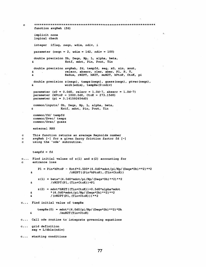
c ****************************************************************** function avgReh (fd)

implicit none logical check

integer iflag, neqn, wdim, ndiv, i

parameter (neqn - 2, wdim - 142, ndiv - 100)

double precision Dh, Deqs, Np, L, alpha, beta, & Kntf, mdot, Pin, Pout, Tin

double precision avgReh, fd, tempfd, seg, xO, xin, xout, & relerr, abserr, rler, aber, PI, P, T, & ReSum, rN2PT, hN2T, muN2T, kPtoP, ctoK, pi

double precision z(neqn), tempz(neqn), guess(neqn), ptvec(neqn), & work(wdim), tempRe(O:ndiv)

parameter (xO - O.OdO, relerr - 1.Od-7, abserr - 1.Od-7) parameter (kPtoP = 1000.OdO, CtoK = 273.l5dO) parameter (pi - 3.l4l592654dO)

common/inputs/ Dh, Deqs, Np, L, alpha, beta, & Kntf, mdot, Pin, Pout, Tin

common/fd/ tempfd common/Zvec/ tempz common/Gvec/ guess

external RHS

c This function returns an average Reynolds number c avgReh [-1 for a given Darcy friction factor fd [-1 c using the 'ode' subroutine.

tempfd - fd

c ... Find initial values of z(l) and z(2) accounting for c entrance loss

PI - Pin*kPtoP - Kntf*0.5DO*(4.0dO*mdot/pi/Np/(Deqs*Dh)**2)**2 & /rN2PT( (Pin*kPtoP), (Tin+CtoK»

z(l) - beta*(4.0dO*mdot/pi/Np/(Deqs*Dh)**2)**2 & /rN2PT(Pl, (Tin+CtoK»+Pl

z(2) - mdot*hN2T«Tin+CtoK»+O.5dO*alpha*mdot & * (4.0dO*mdot/pi/Np/(Deqs*Dh)**2)**2 & / (rN2PT (PI, (Tin+CtoK») **2

c ... Find initial value of tempRe

tempRe(O) &

mdot*(4.0dO/pi/Np/(Deqs*Dh)**2)*Dh /muN2T(Tin+CtoK)

c ... Call ode routine to· integrate governing equations

c ... grid definition seg = L/dble(ndiv)

c .•• starting conditions

77

iflag - 1 xin - xO xout xin + seg rler relerr aber abserr

c ... initialize guess vector needed for newt routine guess (1) P1 guess (2) - Tin+CtoK

c ... calling loop do 20 i = 1, ndiv, 1

10 call ode (RHS, neqn, z, xin, xout, rler, aber, iflag, work)

if (iflag .eq. 3) then print*, 'ode:' print*, 'integration did not reach L because error' print*, 'tolerances too small. relerr, abserr increased' print*, 'appropriately for continuing' goto 10

else if (iflag .eq. 4) then print*, 'ode:' print*, 'integration did not reach L because more' print*, 'than 500 steps needed' stop

else if (iflag .eq. 5) then print*, 'ode:' print*, 'integration did not reach L because equations' print*, 'ap~ear to be stiff' stop

else if (iflag .eq. 6) then print*, 'ode:' print*, 'invalid input parameters (fatal error)' stop

endif

c ... Find P and T from the values of z(l) and z(2)

tempz(l) z(l) tempz(2) z(2)

c. .. provide guess values c (see funcv routine for explanation of ptvec)

ptvec(l) ptvec(2)

guess (l)/(Pin*kPtoP) guess (2)/(Tin+CtoK)

call newt (ptvec, neqn, check) if (check) then

print*, 'newt:' print*, 'the routine has converged to a local minimum' print*, 'of the function fmin. Try restarting from a' print*, 'different initial guess.' stop

endif

P ptvec(l) * (Pin*kPtoP) T ptvec(2) * (Tin+CtoK)

c ... Find tempRe(i) from values of P and T tempRe(i) mdot*(4.0dO/pi/Np/(Deqs*Dh)**2)*Dh/muN2T(T)

c ... Move to next segment

78

xout - xin + seg

20 continue

c. .. Find avgReh

ReSum - O. OdD do 30 i - 0, ndiv, 1

ReSum - ReSum + tempRe(i) 30 continue

c

avgReh

return end

ReSum/dble(ndiv+l)

****************************************************************** subroutine RHS (x,z,zp)

implicit none logical check integer neqn

parameter (neqn - 2)

double precision Dh, Deqs, Np, L, alpha, beta, & Kntf, mdot, Pin, Pout, Tin

double precision fd, x, P, T, kPtoP, CtoK, pi, rN2PT

double precision z(neqn), tempz(neqn), guess(neqn), zp(neqn), & ptvec (neqn)

parameter (kPtoP - lOOO.OdO, CtoK - 273.l5dO) parameter (pi - 3.l4l592654dO)

common/inputs/ Dh, Deqs, Np, L, alpha, beta, & Kntf, mdot, Pin, Pout, Tin

common/fd/ fd common/Zvec/ tempz c~mmon/Gvec/ guess

c This subroutine is to be supplied to the 'ode' routine. c It calculates the RHS vector of the ODE system.

c ... Find P and T from the values of z(l) and z(2)

tempz(l) z(l) tempz (2) z (2)

c ... provide guess values c (see funcv routine for explanation of ptvec)

ptvec(l) ptvec(2)

guess (l)/(Pin*kPtoP) guess(2)/(Tin+CtoK)

call newt (ptvec, neqn, check)

if (check) then print*, 'newt:' print*, 'the routine has converged to a local minimum'

79

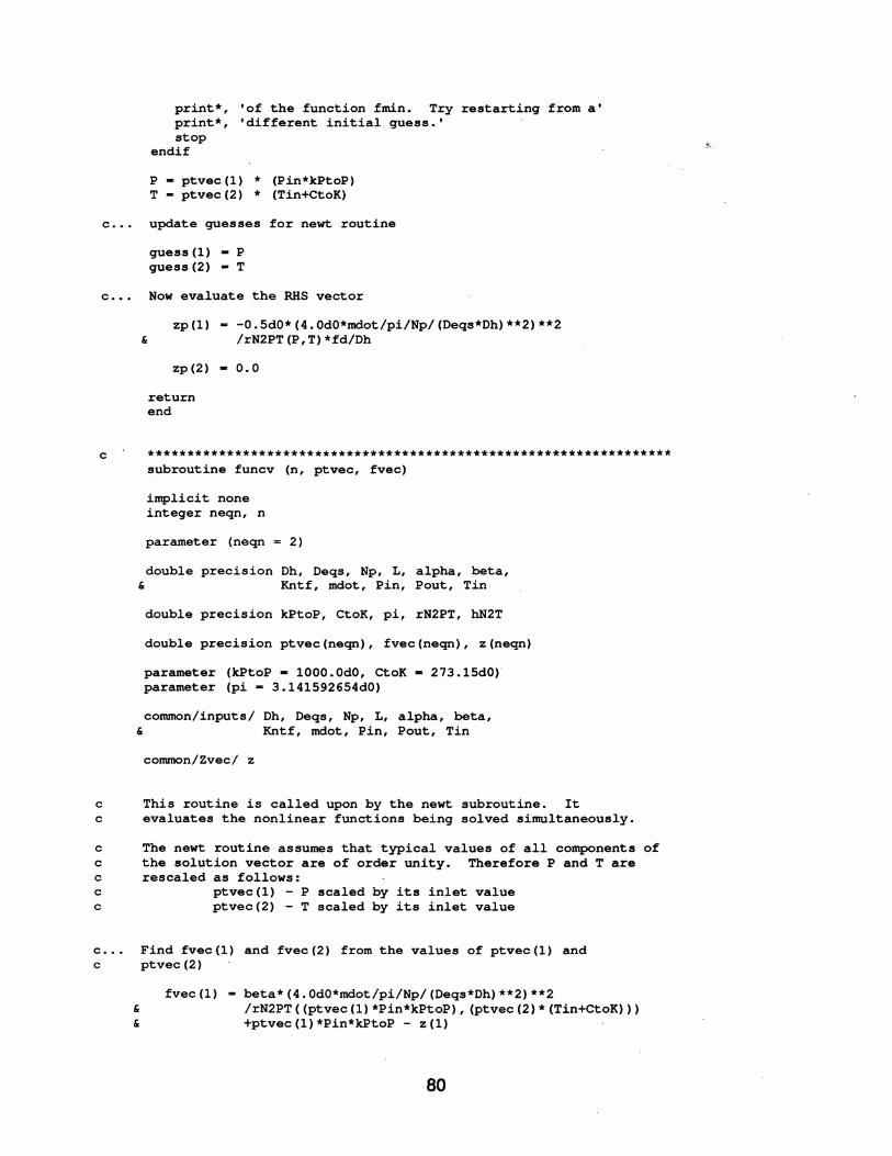
print*, 'of the function fmin. Try restarting from a' print*, 'different initial guess.' stop

endif

P ptvec(l) * (Pin*kPtoP) T ptvec(2) * (Tin+CtoK)

c .•. update guesses for newt routine

guess(l) P guess (2) T

c .•. Now evaluate the RHS vector

zp(l) - -0.5dO*(4.0dO*mdot/pi/Np/(Deqs*Dh)**2)**2 & /rN2PT(P,T)*fd/Dh

zp(2) 0.0

return end

c ****************************************************************** subroutine funcv (n, ptvec, fvec)

implicit none integer neqn, n

parameter (neqn = 2)

double precision Dh, Deqs, Np, L, alpha, beta, & Kntf, mdot, Pin, Pout, Tin

double precision kPtoP, CtoK, pi, rN2PT, hN2T

double precision ptvec(neqn), fvec(neqn), z(neqn)

parameter (kPtoP - lOOO.OdO, CtoK - 273.l5dO) parameter (pi - 3.l41592654dO)

common/inputs/ Dh, Deqs, Np, L, alpha, beta, & Kntf, mdot, Pin, Pout, Tin

common/Zvec/ z

c This routine is called upon by the newt subroutine. It c evaluates the nonlinear functions being solved simultaneously.

c The newt routine assumes that typical values of all components of c the solution vector are of order unity. Therefore P and Tare c rescaled as follows: c ptvec(l) P scaled by its inlet value c ptvec (2) - T scaled by its inlet value

c ... Find fvec(l) and fvec(2) from the values of ptvec(l) and c ptvec (2)

& &

fvec(l) beta*(4.0dO*mdot/pi/Np/(Deqs*Dh)**2)**2 /rN2PT«ptvec(l)*Pin*kPtoP), (ptvec(2)*(Tin+CtoK») +ptvec(l)*Pin*kPtoP - z(l)

80

c

c

& & &

fvec(2) - mdot*hN2T (ptvec (2) * (Tin+CtoK» +0.5dO*alpha*mdot*(4.0dO*mdot/pi/Np/(Deqs*Dh)**2)**2

/(rN2PT«ptvec(1)*Pin*kPtoP), (ptvec(2)*(Tin+CtoK»»**2 - z(2)

return end

****************************************************************** function findx (f,value,ax,bx,relerr,abserr)

implicit none double precision findx,ax,bx,f,value,relerr,abserr external f

c ... solves the equation f(x) - value in the interval (ax,bx) c c... input c c f - name of function subprogram which computes f(x) c (must be declared EXTERNAL in calling program) c value rhs of equation, i.e., f(x) - value c ax left endpoint of initial interval c bx right endpoint of initial interval c reI err allowable relative error in x c abserr allowable absolute error in x c c... output c c findx = approximate zero c c •.. findx returns a zero in the given interval (ax, bx) to a tolerance c of (relerr+4*macheps) *abs (x) + abserr, where macheps is the relative c machine precision and x is the value of the zero. c

c

save toll double precision a,b,c,d,e,eps,fa,fb,fc,toll,xm,p,q,r,s double precision rerror data toll/O.OdO/

c ... compute eps, the relative machine precision c

c

if (toll. eq. O. OdO) then eps-l.OdO

10 eps-eps/2.0dO toll-l.OdO+eps if (toll.gt.l.OdO) go to 10

endif

c ... initialization c

a-ax b-bx fa-f(a) - value fb-f(b) - value if (fa*fb.gt.O.OdO) then

print * , 'findx:' print*, 'answer not contained within the initial interval' print*, 'setting findx equal to the closer boundary.' print*, 'Make sure you have a way of handling this error.' print * , 'lower boundary , ax print*, 'upper boundary - " bx

81

c

if (abs(fa) .It. abs(fb» then findx ax

else findx bx

endif print * , , findx print * return

findx

endif rerror-relerr+2.0dO*eps

c ... begin step c

c

20 c-a fc-fa d-b-a e-d

30 if (abs(fc).ge.abs(fb» go to 40 a-b b-c c-a fa-fb fb-fc fc-fa

c ••• convergence test c

c

40 toll-rerror*abs(b)+0.5dO*abserr xm=0.5dO*(c-b) if (abs(xm) .le.toll) go to 90 if (fb.eq.O.O) go to 90

c .•• is bisection necessary c

if (abs(e).lt.toll) go to 70 if (abs(fa).le.abs(fb» go to 70

c c ... is quadratic interpolation possible c

if (a.ne.c) go to 50 c c ••. linear interpolation c

c

s-fb/fa p-2.0dO*xm*s q-l.OdO-s go to 60

c •.. inverse quadratic interpolation c

50 q-fa/fc r-fb/fc s-fb/fa p-s*(2.0dO*xm*q* (q-r)-(b-a) * (r-l.OdO» q-(q-l.OdO) * (r-l.OdO) *(s-l.OdO)

c c .•• adjust signs c

c

60 if (p.gt.O.OdO) q--q p-abs(p)

c ••• is interpolation acceptable c

if «2.0dO*p) .ge. (3.0dO*xm*q-abs(toll*q») go to 70

82

~ .. -

c

if (p.ge.abs(0.5dO*e*q» go to 70 e-d d-p/q go to 80

c. .• bisection c

c

70 d-xm e-d

c .•• complete step c

80 a-b fa-fb if (abs(d).gt.tol1) b-b+d if (abs(d).le.tol1) b-b+sign(tol1,xm) fb-f(b) - value if «fb*(fc/abs(fc»).gt.O.O) go to 20 go to 30

c c... done c

90 findx-b return end

c ****************************************************************** function rN2PT(P,TK)

implicit none double precision rN2PT,R,P,TK parameter (R - 296.82256dO)

c This function returns the density as a function of pressure and c temperature for N2.

c Assumed units are c P [Pal c R [J/kg-K] c TK [K] c rho [kg/mA 3]

rN2PT

return end

P / R / TK

c ****************************************************************** function muN2T(TK)

implicit none double precision muN2T,TK,muO,TKO,S parameter (muO - 1.663d-5, TKO - 273.0dO, S - 107.0dO)

c This function returns the viscosity of N2 given temperature c using the Sutherland-law for dilute gases. The necessary c constants are found on p. 29 of

c White, Viscous Fluid Flow ,2nd Edition, McGraw-Hill, c New York, 1991.

c Assumed units are

83

~'.

c muN2T [Pa*s] c TK [K]

muN2T

return end

muO*«TK/TKO)**(1.5»*(TKO+S)/(TK+S)

c ****************************************************************** function hN2T(TK)

implicit none double precision hN2T,TK

c This function returns the ideal gas enthalpy [J/kg] given c temperature for Nitrogen

double precision N2integrand external N2integrand double precision TO,abserr,relerr,result,errest,flag integer nofun parameter (TO-300.0dO, abserr-l.Od-10, relerr-l.Od-10)

c Here we integrate from the assumed zero for enthalpy, 300K, c to the desired temperature, TK. Note that the quanc8 routine c uses the following input and output parameters.

c c c c c c c c c c c c c c c c c c c

input

fun a b abserr relerr

output

result

errest no fun flag

the name of the integrand function subprogram fun(x). the lower limit of integration. the upper limit of integration. (b may be less than a.) an absolute error tolerance. (should be non-negative) a relative error tolerance. (should be non-negative)

an approximation to the integral hopefully satisfying the least stringent of the two error tolerances. an estimate of the magnitude of the actual error. the number of function values used in calculation of result. a reliability indicator. if flag is zero, then result probably satisfies the error tolerance. if flag is xxx.yyy , then xxx - the number of intervals which have not converged and O.yyy - the fraction of the interval left to do when the limit on nofun was approached.

call quanc8(N2integrand,TO,TK,abserr,relerr, & result,errest,nofun,flag)

c If we have a problem, print out the value of flag if (flag .ne. O.OdO) then

print* print*, 'There has been a problem with the evaluation of' print*, 'the ideal gas integral for enthalpy in function hN2T.' print*, 'You should check the comments in the function to' print*, 'find out what this value of flag means.' print*, ", flag - " flag print*

endif

c Reassign the function value [J/kg]

84

~'.

c

hN2T - result * 1000.0dO

return end

****************************************************************** function N2integrand(TK)

implicit none double precision N2integrand,TK

c This function returns the integrand for the ideal gas enthalpy c for Nitrogen. Equation for CpObar from p. 652 of

c Sonntag and VanWylen, Fundamentals of Classical Thermodynamics , c 3rd Edition, Wiley, New York, 1985.- - - -

c The equation for CpObar is good for the range c 300 < TK < 3500.

c The plan is to evaluate the equation c T c integral CpO dT c ~

c so this function returns CpO

double precision cO,c1,c2,c3,MWN2 parameter (cO-39.060dO, c1--512.79dO, c2-1072.7dO, c3--820.40dO) parameter (MWN2 - 28.013dO) double precision theta,CpObar,CpO

theta - TK / 100.0dO c CpObar in kJ/kmol-K

CpObar - cO + c1/theta**1.5 + c2/theta**2.0 + c3/theta**3.0

c Now calculate CpO CpO - CpObar / MWN2

c And finally, the integrand, CpO N2integrand - CpO

return end

c ******************************************************************

c

subroutine quanc8 (fun,a,b,abserr,relerr,result,errest,nofun,flagJ implicit none double precision fun,a,b,abserr,relerr,result,errest,flag integer nofun

c estimate the integral of fun (x) from a to b c to a user provided tolerance. c an automatic adaptive rou~ine based on c the 8-panel newton-cotes rule. c c input c c c c

fun a b

the name of the integrand function subprogram fun(x). the lower limit of integration. the upper limit of integration. (b may be less than a.)

85

c c c c c c c c c c c c c c c

c c c c

c

relerr abserr

output

result

errest nofun flag

a relative error tolerance. (should be non-negative) an absolute error tolerance. (should be non-negative)

an approximation to the integral hopefully satisfying the least stringent of the two error tolerances. an estimate of the magnitude of the actual error. the number of function values used in calculation of result. a reliability indicator. if flag is zero, then result probably satisfies the error tolerance. if flag is xxx.yyy , then xxx - the number of intervals which have not converged and O.yyy - the fraction of the interval left to do when the limit on nofun was approached.

double precision wO,w1,w2,w3,w4,area,xO,fO,stone,step,cor11,temp double precision qprev,qnow,qdiff,qleft,esterr,tolerr double prec~s~on qright(31),f(16),x(16),fsave(8,30),xsave(8,30) integer levrnin,levmax,levout,nomax,nofin,lev,nim,i,j

*** stage 1 *** set constants.

levrnin=1 levmax-30 levout-6

general initialization

nomax'"'5000 nofin-nomax-8*(levmax-levout+2**(levout+1»

c trouble when nofun reaches nofin c

c

wO=3956.0/14175.0 w1-23552.0/14175.0 w2--3712.0/14175.0 w3-41984.0/14175.0 w4--18160.0/14175.0

c initialize running sums to zero. c

c c c

flag-O.O result-O.O cor11-0.0 errest-O.O area-O.O nofun-O if (a.eq.b) return

*** stage 2 *** initialization for first interval

lev-O nim=1 xO-a x (16)"'b qprev-O.O fO-fun(xO) stone-(b-a)/16.0 x(8)-(xO+x(16»/2.0 x(4)-(xO+x(8»/2.0 x(12)-(x(8)+x(16»/2.0 x(2)-(xO+x(4»/2.0 x(6)-(x(4)+x(8»/2.0 x(10)-(x(8)+x(12»/2.0 x(14)-(x(12)+x(16»/2.0 do 25 j-2,16,2

86

c

f (j)-fun (x(j» 25 continue

nofun-9

c *** stage 3 *** central calculation c requires qprev,xO,x2,x4, •.• ,x16,fO,f2,f4, .•. ,f16. c calculates x1,x3, ... x15, f1,f3, ..• f15,qleft,qright,qnow,qdiff,area. c

c c c

c

30 x(1)-(xO+x(2»/2.0 f(l)-fun(x(l» do 35 j-3,15,2

x(j)-(x(j-1)+x(j+1»/2.0 f (j) -fun (x (j»

35 continue nofun-nofun+8 step-(x(16)-xO)/16.0 qleft-(wO*(fO+f(8»+w1*(f(1)+f(7»+w2*(f(2)+f(6»+w3*(f(3)+f(5»+w

14*f(4»*step qright(lev+1)-(wO*(f(8)+f(16»+w1*(f(9)+f(15»+w2*(f(10)+f(14»+w3

1*(f(11)+f(13»+w4*f(12»*step qnow-qleft+qright(lev+1) qdiff-qnow-qprev area-area+qdiff

*** stage 4 *** interval convergence test

esterr-abs(qdiff)/1023.0 tolerr-amax1 (abserr,relerr*abs(area»* (step/stone) if (lev.lt.levmin) go to 50 if (lev.ge.levmax) go to 62 if (nofun.gt.nofin) go to 60 if (esterr.le.tolerr) go to 70

c *** stage 5 *** no convergence c locate next interval. c

c

50 nim-2*nim lev-lev+1

c store right hand elements for future use. c

c

do 52 i-1,8 fsave(i,lev)-f(i+8) xsave(i,lev)-x(i+8)

52 continue

c assemble left hand elements for immediate use. c

c

qprev-qleft do 55 i-1,8

j--i f(2*j+18)-f(j+9) x(2*j+18)-x(j+9)

55 continue go to 30

c *** stage 6 *** trouble section c number of function values is about to exceed limit. c

c

60 nofin-2*nofin levmax-levout flag-flag+(b-xO)/(b-a) go to 70

87

c current level is levmax. c

62 flag-flag+1.0 c c *** stage 7 *** interval converged c add contributions into running sums. c

c

70 result-result+qnow errest-errest+esterr cor11-cor11+qdiff/1023.0

c locate next interval. c

c

72 if (nim.eq.2*(nim/2» go to 75 nim-nim/2 lev-lev-1 go to 72

75 nim-nim+1 if (lev.le.O) go to 80

c assemble elements required for the next interval. c

c c c

c

qprev-qright(lev) xO-x(16) fO-f(16) do 78 i-1,8

f(2*i)-fsave(i,lev) x(2*i)-xsave(i,lev)

78 continue go to 30

*** stage 8 *** finalize and return

80 result-result+cor11

c make sure errest not less than roundoff level. c

if (errest.eq.O.O) return 82 temp-abs(result)+errest

if (temp.ne.abs(result» return errest-2.0*errest go to 82 end

88

~ .. -

REFERENCES

Ahmed, S., and Brundrett, E. (1971), -Characteristic Lengths for Non-Circular Ducts: Int. J. Heat Mass Transfer, Vol. 14, pp. 157-159.

AI-Arabi, M. (1982), -Turbulent Heat Transfer in the Entrance Region of a Tube: Heat Transfer Eng., Vol. 3, pp. 76-83.

Andres, D. J. (1994), Design and Construction of a Condensation Hea~ Transfer Experimental Facility for use with Microchannel Condenser Tubing, University of Illinois, Urbana-Champaign, M. S. Thesis.

Bhatti, M. S., and Shah, R. K. (1987), Turbulent and Transition Flow Convective Heat Transfer in Ducts, Ch. 4 in Handbook of Single-Phase Convective Heat Transfer (eds. Kakac, S., Shah, R. K., and Aung, W.), Wiley-Interscience, New York.

Bradshaw, P. (1977), Compressible Turbulent Shear Layers, Ann. Rev. Fluid Mech., Annual Reviews, Inc.

Chen, R. Y. (1973), -Flow in the Entrance Region at Low Reynolds Numbers, - J. Fluids Eng., Vol. 95, pp. 153-158.

Churchill, S. W. (1977a), -Friction-Factor Equation Spans All Fluid-Flow Regimes,­Chemical Engineering .. Vol. 84, pp. 91--92.

Churchill, S. W. (1977b), -Comprehensive Correlating Equations for Heat, Mass, and Momentum Transfer in Fully Developed Flow in Smooth Tubes: Ind. Eng. Chem. Fundam., Vol. 16, No.1, pp. 109-116.

Colburn, A. P. (1933), -A Method of Correlating Forced Convection Heat Transfer Data and a Comparison With Auid Friction: Trans. AIChE, Vol. 19, pp. 174-210.

Colebrook, C. F. (1939), -Turbulent Flow in Pipes with Particular Reference to the Transition Region between the Smooth and Rough Pipes Laws, - J. Inst. Civ. Eng., Vol. 11, pp.133-156.

Dittus, P. W., and Boelter, L. M. K. (1930), -Heat Transfer in Automobile Radiators of the Tubular Type, - Univ. Calif Pub. Eng., Vol. 2, No. 13, pp. 443-461.

Eckert, E. R., and Irvine, T. F. (1957), -Incompressible Friction Factor, Transition, and Hydrodynamic Entrance-Length Studies of Ducts with Triangular and Rectangular Cross Sections, - Proceedings of the 5th Midwestern Conference on Fluid Mechanics, University of Michigan Press, pp.122-145.

Filonenko, G. K. (1954), -HydrauliC Resistance in Pipes: Teploenergetika, Vol. 1, No.4, pp.40-44.

Gnielinski, V. (1976), -New Equations for Heat and Mass Transfer in Turbulent Pipe and Channel Flow, - Int. Chem Eng., Vol. 16, pp. 359-368.

89

Graetz, L. (1883), "On the Thermal Conductivity of Liquids," Ann. Phys. Chem., Vol. 18, pp.337-357.

Hausen, H. (1943), "Darstellung des WarmeOberganges in Rohren durch verallgemeinerte Potenzbeziehungen," VOl Z, Suppl. "Verfahrenstecchnik," No.4, pp.91-98.

Heun, M. K. (1995), Performance and Optimization of Microchannel Condensers, University of Illinois, Urbana-Champaign, Ph.D Thesis.

Incropera, F. P., and DeWitt, D. P. (1990), Fundamentals of Heat and Mass Transfer, 3rd ed., Wiley & Sons, New York.

Jones, O. C. (1976), "An Improvement in the Calculation of Turbulent Friction in Rectangular Ducts," J. Fluids Eng., Vol. 98, pp. 173-181.

Leutheusser, H. J. (1963), "Turbulent Flow in Rectangular Ducts," ASCE, Journal of the Hydraulics Division 89, HY3.

Luhrs, D. A. (1994), Design and Construction of a Microchannel Condenser Tube Experimental Facility, University of Illinois, Urbana-Champaign, M. S. Thesis.

Lundgren, T. S., Sparrow, E. M., and Starr,J. B. (1964), "Pressure Drop Due to the Entrance Region in Ducts of Arbitrary Cross Section," J. Basic Eng., Vol. 86, pp. 620-626.

Mason, J. L. (1954), "Heat Transfer in Crossflow," Proceedings of the U. S. National Congress on Applied Mechanics, pp. 801-803.

Miller, R. W., and Han, L. S. (1971), "Pressure Losses for Laminar Flow in the Entrance Region of Ducts of Rectangular and Equilateral Triangular Cross Sections," J. Appl. Mech., Vol. 38, pp. 1083-1087.

Nikuradse, J. (1932), "Gesetzma~igkeiten der turbulenten Stromung in glatten Rohren," Forsch. Arb. Ing.-Wes., No. 356; English transl., NASA IT F-10, 359,1966.'

Nikuradse, J. (1933), "Stromungsgesetze in rauhen Rohren," Forsch. Arb. Ing.-Wes., No. 361; English transl., NACA TM 1292.

Norris, R. H. (1970), "Some Simple Approximate Heat Transfer Correlations for Turbulent Flow in Ducts with Rough Surfaces," Augmentation of Convective Heat and Mass Transfer, ASME, New York.

Obot, N. T. (1988), "Determination of Incompressible Flow Friction in Smooth Circular and Noncircular Passages: A Generalized Approach Including Validation of the Nearly Century-Old HydrauliC Diameter Concept," J. Fluids Eng., Vol. 110, pp. 431-440.

Obot, N. T. (1993), "The Frictional Law of Corresponding States: Its Origin and Applications," Trans. IChemE, Vol. 71, Part A, pp. 3-10.

90

Olsson, C. (1994), "Pressure Drop Characteristics of Small-Sized Tubes," ASME, New York.

1".

Petukhov, B. S., Kurganov, V. A., and Gladuntsov, A. I. (1973), "Heat Transfer in Turbulent Pipe Flow of Gases with Variable Properties," Heat Transfer Sov. Ref. 5, No.4,pp.109--116.

Press, W. H., Teukolsky, S. A., Vetterling, W. T., and Flannery, B. P. (1992), Numerical ReCipes in FORTRAN, 2nd ed., Cambridge University Press, New York.

Shah, R. K., and London, A. L. (1978), Laminar Flow Forced Convection in Ducts, Advances in Heat Transfer, suppl. 1, Academic Press, New York.

Shah, R. K., and Bhatti, M. S. (1987), Laminar Convective Heat Transfer in Ducts, Ch. 3 in Handbook of Single-Phase Convective Heat Transfer (eds. Kakac, S., Shah, R. K., and Aung, W.), Wiley-Interscience, New York.

Shampine, L. F., and Gordon, M. K. (1975), Computer Solutions of Ordinary Differential Equations: The Initial Value Problem, W. H. Freeman, San Francisco.

Stoecker, W. F., and Jones, J. W. (1982), Refrigeration and Air Conditioning, 2nd ed., McGraw-Hili, New York.

White, F. M. (1987), Fluid Mechanics, 2nd ed., McGraw-Hili, New York.

Wilson, N. W., and Azad, R. S. (1975), "A Continuous Prediction Method for Fully Developed Laminar, Transitional and Turbulent Flows in Pipes," J. Applied Mech., Vol. 42, pp. 51-54.

Zhi-qing, W. (1982), "Study on Correction Coefficients of Laminar and Turbulent Entrance Region Effect in Round Pipe, II Appl. Math. Mech., Vol. 3, No.3, pp. 433-446.

91