Frequentist Consistencyof Variational Bayes

Yixin WangDepartment of Statistics

Columbia Universityyixin.wang@columbia.edu

David M. BleiDepartment of Statistics

Department of Computer ScienceColumbia University

david.blei@columbia.edu

May 25, 2018

Abstract

A key challenge for modern Bayesian statistics is how to perform scalable inference of pos-terior distributions. To address this challenge, variational Bayes (VB) methods have emergedas a popular alternative to the classical Markov chain Monte Carlo (MCMC) methods. VBmethods tend to be faster while achieving comparable predictive performance. However, thereare few theoretical results around VB. In this paper, we establish frequentist consistency andasymptotic normality of VB methods. Specifically, we connect VB methods to point esti-mates based on variational approximations, called frequentist variational approximations, andwe use the connection to prove a variational Bernstein–von Mises theorem. The theorem lever-ages the theoretical characterizations of frequentist variational approximations to understandasymptotic properties of VB. In summary, we prove that (1) the VB posterior converges tothe Kullback-Leibler (KL) minimizer of a normal distribution, centered at the truth and (2)the corresponding variational expectation of the parameter is consistent and asymptoticallynormal. As applications of the theorem, we derive asymptotic properties of VB posteriors inBayesian mixture models, Bayesian generalized linear mixed models, and Bayesian stochasticblock models. We conduct a simulation study to illustrate these theoretical results.

Keywords: Bernstein–von Mises, Bayesian inference, variational methods, consistency, asymp-totic normality, statistical computing

1

arX

iv:1

705.

0343

9v2

[st

at.M

L]

24

May

201

8

1 Introduction

Bayesian modeling is a powerful approach for discovering hidden patterns in data. We begin bysetting up a probability model of latent variables and observations. We incorporate prior knowledgeby setting priors on latent variables and a functional form of the likelihood. Finally we infer theposterior, the conditional distribution of the latent variables given the observations.

For many modern Bayesian models, exact computation of the posterior is intractable and statis-ticians must resort to approximate posterior inference. For decades, Markov chain Monte Carlo(MCMC) sampling (Hastings, 1970; Gelfand and Smith, 1990; Robert and Casella, 2004) hasmaintained its status as the dominant approach to this problem. MCMC algorithms are easy to useand theoretically sound. In recent years, however, data sizes have soared. This challenges MCMCmethods, for which convergence can be slow, and calls upon scalable alternatives. One popularclass of alternatives is variational Bayes (VB) methods.

To describe VB, we introduce notation for the posterior inference problem. Consider observationsx = x1:n. We posit local latent variables z = z1:n, one per observation, and global latent variablesθ = θ1:d. This gives a joint,

p(θ, x, z)= p(θ)n∏

i=1p(zi |θ)p(xi | zi,θ). (1)

The posterior inference problem is to calculate the posterior p(θ, z |x).

This division of latent variables is common in modern Bayesian statistics.1 In the Bayesian Gaus-sian mixture model (GMM) (Roberts et al., 1998), the component means, covariances, and mixtureproportions are global latent variables; the mixture assignments of each observation are local latentvariables. In the Bayesian generalized linear mixed model (GLMM) (Breslow and Clayton, 1993),the intercept and slope are global latent variables; the group-specific random effects are local latentvariables. In the Bayesian stochastic block model (SBM) (Hofman and Wiggins, 2008), the clus-ter assignment probabilities and edge probabilities matrix are two sets of global latent variables;the node-specific cluster assignments are local latent variables. In the latent Dirichlet allocation(LDA) model (Blei et al., 2003), the topic-specific word distributions are global latent variables;the document-specific topic distributions are local latent variables. We will study all these exam-ples below.

VB methods formulate posterior inference as an optimization (Jordan et al., 1999; Wainwright andJordan, 2008; Blei et al., 2016). We consider a family of distributions of the latent variables andthen find the member of that family that is closest to the posterior.

Here we focus on mean-field variational inference (though our results apply more widely). First,we posit a family of factorizable probability distributions on latent variables

Qn+d ={

q : q(θ, z)=∏di=1 qθi (θi)

∏nj=1 qz j (z j)

}.

1In particular, our results are applicable to general models with local and global latent variables (Hoffman et al.,2013). The number of local variables z increases with the sample size n; the number of global variables θ does not. Wealso note that the conditional independence of Equation (1) is not necessary for our results. But we use this commonsetup to simplify the presentation.

2

This family is called the mean-field family. It represents a joint of the latent variables with n+d(parametric) marginal distributions, {qθ1 , . . . , qθd , qz1 , . . . , qzn}.

VB finds the member of the family closest to the exact posterior p(θ, z |x), where closeness ismeasured by KL divergence. Thus VB seeks to solve the optimization,

q∗(θ, z)= argminq(θ,z)∈Qn+d

KL(q(θ, z) || p(θ, z | x)). (2)

In practice, VB finds q∗(θ, z) by optimizing an alternative objective, the evidence lower bound(ELBO),

ELBO(q(θ, z))=−∫

q(θ, z) logq(θ, z)

p(θ, x, z)dθdz. (3)

This objective is called the ELBO because it is a lower bound on the evidence log p(x). Moreimportantly, the ELBO is equal to the negative KL plus log p(x), which does not depend on q(·).Maximizing the ELBO minimizes the KL (Jordan et al., 1999).

The optimum q∗(θ, z) = q∗(θ)q∗(z) approximates the posterior, and we call it the VB posterior.2

Though it cannot capture posterior dependence across latent variables, it has hope to capture eachof their marginals. In particular, this paper is about the theoretical properties of the VB posteriorq∗(θ), the VB posterior of θ. We will also focus on the corresponding expectation of the globalvariable, i.e., an estimate of the parameter. It is

θ∗n :=∫θ · q∗(θ)dθ.

We call θ∗ the variational Bayes estimate (VBE).

VB methods are fast and yield good predictive performance in empirical experiments (Blei et al.,2016). However, there are few rigorous theoretical results. In this paper, we prove that (1) the VBposterior converges in total variation (TV) distance to the KL minimizer of a normal distributioncentered at the truth and (2) the VBE is consistent and asymptotically normal.

These theorems are frequentist in the sense that we assume the data come from p(x, z ; θ0) with atrue (nonrandom) θ0. We then study properties of the corresponding posterior distribution p(θ |x),when approximating it with variational inference. What this work shows is that the VB posterioris consistent even though the mean field approximating family can be a brutal approximation. Inthis sense, VB is a theoretically sound approximate inference procedure.

1.1 Main ideas

We describe the results of the paper. Along the way, we will need to define some terms: thevariational frequentist estimate (VFE), the variational log likelihood, the VB posterior, the VBE,and the VB ideal. Our results center around the VB posterior and the VBE. (Table 1 contains aglossary of terms.)

2For simplicity we will write q(θ, z)=∏di=1 q(θi)

∏nj=1 q(z j), omitting the subscript on the factors q(·). The under-

standing is that the factor is indicated by its argument.

3

The variational frequentist estimate (VFE) and the variational log likelihood. The first ideathat we define is the variational frequentist estimate (VFE). It is a point estimate of θ that max-imizes a local variational objective with respect to an optimal variational distribution of the localvariables. (The VFE treats the variable θ as a parameter rather than a random variable.) We callthe objective the variational log likelihood,

Mn(θ ; x)=maxq(z)

Eq(z) [log p(x, z |θ)− log q(z)] . (4)

In this objective, the optimal variational distribution q†(z) solves the local variational inferenceproblem,

q†(z)= argminq

KL(q(z) || p(z |x,θ)). (5)

Note that q†(z) implicitly depends on both the data x and the parameter θ.

With the objective defined, the VFE is

θn = argmaxθ

Mn(θ ; x). (6)

It is usually calculated with variational expectation maximization (EM) (Wainwright and Jordan,2008; Ormerod and Wand, 2010), which iterates between the E step of Equation (5) and the M stepof Equation (6). Recent research has explored the theoretical properties of the VFE for stochas-tic block models (Bickel et al., 2013), generalized linear mixed models (Hall et al., 2011b), andGaussian mixture models (Westling and McCormick, 2015).

We make two remarks. First, the maximizing variational distribution q†(z) of Equation (5) is dif-ferent from q∗(z) in the VB posterior: q†(z) is implicitly a function of individual values of θ, whileq∗(z) is implicitly a function of the variational distributions q(θ). Second, the variational log like-lihood in Equation (4) is similar to the original objective function for the EM algorithm (Dempsteret al., 1977). The difference is that the EM objective is an expectation with respect to the exactconditional p(z |x), whereas the variational log likelihood uses a variational distribution q(z).

Variational Bayes and ideal variational Bayes. While earlier applications of variational infer-ence appealed to variational EM and the VFE, most modern applications do not. Rather theyuse VB, as we described above, where there is a prior on θ and we approximate its posteriorwith a global variational distribution q(θ). One advantage of VB is that it provides regularizationthrough the prior. Another is that it requires only one type of optimization: the same considerationsaround updating the local variational factors q(z) are also at play when updating the global factorq(θ).

To develop theoretical properties of VB, we connect the VB posterior to the variational log likeli-hood; this is a stepping stone to the final analysis. In particular, we define the VB ideal posteriorπ∗(θ |x),

π∗(θ |x)= p(θ)exp{Mn(θ ; x)}∫p(θ)exp{Mn(θ ; x)}dθ

. (7)

4

Here the local latent variables z are constrained under the variational family but the global latentvariables θ are not. Note that because it depends on the variational log likelihood Mn(θ ; x), thisdistribution implicitly contains an optimal variational distribution q†(z) for each value of θ; seeEquations (4) and (5).

Loosely, the VB ideal lies between the exact posterior p(θ |x) and a variational approximation q(θ).It recovers the exact posterior when p(z |θ, x) degenerates to a point mass and q†(z) is always equalto p(z |θ, x); in that case the variational likelihood is equal to the log likelihood and Equation (7) isthe posterior. But q†(z) is usually an approximation to the conditional. Thus the VB ideal usuallyfalls short of the exact posterior.

That said, the VB ideal is more complex that a simple parametric variational factor q(θ). Thereason is that its value for each θ is defined by the optimization within Mn(θ ; x). Such a distributionwill usually lie outside the distributions attainable with a simple family.

In this work, we first establish the theoretical properties of the VB ideal. We then connect it to theVB posterior.

Variational Bernstein–von Mises. We have set up the main concepts. We now describe the mainresults.

Suppose the data come from a true (finite-dimensional) parameter θ0. The classical Bernstein–vonMises theorem says that, under certain conditions, the exact posterior p(θ |x) approaches a normaldistribution, independent of the prior, as the number of observations tends to infinity. In this paper,we extend the theory around Bernstein–von Mises to the variational posterior. Here we summarizeour results.

• Lemma 1 shows that the VB ideal π∗(θ |x) is consistent and converges to a normal distributionaround the VFE. If the VFE is consistent, the VB ideal π∗(θ | x) converges to a normal dis-tribution whose mean parameter is a random vector centered at the true parameter. (Note therandomness in the mean parameter is due to the randomness in the observations x.)

• We next consider the point in the variational family that is closest to the VB ideal π∗(θ | x) in KLdivergence. Lemma 2 and Lemma 3 show that this KL minimizer is consistent and convergesto the KL minimizer of a normal distribution around the VFE. If the VFE is consistent (Bickelet al., 2013; Hall et al., 2011b) then the KL minimizer converges to the KL minimizer of anormal distribution with a random mean centered at the true parameter.

• Lemma 4 shows that the VB posterior q∗(θ) enjoys the same asymptotic properties as the KLminimizers of the VB ideal π∗(θ |x).

• Theorem 5 is the variational Bernstein–von Mises theorem. It shows that the VB posterior q∗(θ)is asymptotically normal around the VFE. Again, if the VFE is consistent then the VB posteriorconverges to a normal with a random mean centered at the true parameter. Further, Theorem 6shows that the VBE θ∗n is consistent with the true parameter and asymptotically normal.

• Finally, we prove two corollaries. First, if we use a full rank Gaussian variational family then thecorresponding VB posterior recovers the true mean and covariance. Second, if we use a mean-field Gaussian variational family then the VB posterior recovers the true mean and the marginalvariance, but not the off-diagonal terms. The mean-field VB posterior is underdispersed.

5

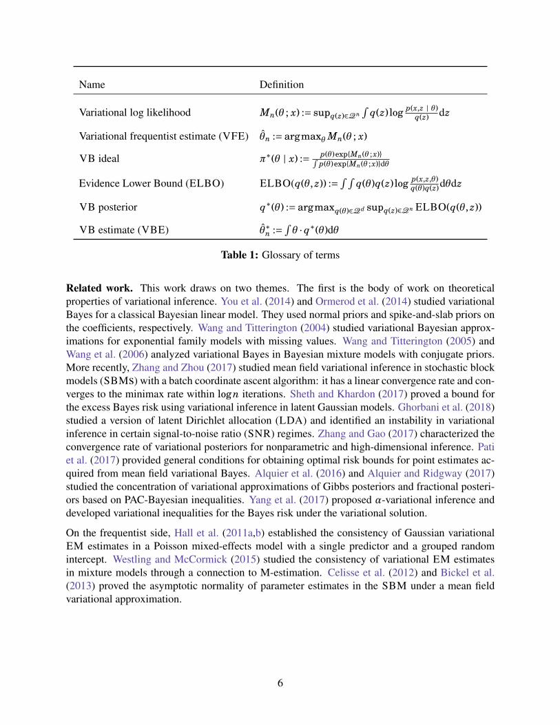
Name Definition

Variational log likelihood Mn(θ ; x) := supq(z)∈Qn∫

q(z) log p(x,z | θ)q(z) dz

Variational frequentist estimate (VFE) θn := argmaxθ Mn(θ ; x)

VB ideal π∗(θ | x) := p(θ)exp{Mn(θ ; x)}∫p(θ)exp{Mn(θ ; x)}dθ

Evidence Lower Bound (ELBO) ELBO(q(θ, z)) := ∫ ∫q(θ)q(z) log p(x,z,θ)

q(θ)q(z)dθdz

VB posterior q∗(θ) := argmaxq(θ)∈Qd supq(z)∈Qn ELBO(q(θ, z))

VB estimate (VBE) θ∗n := ∫θ · q∗(θ)dθ

Table 1: Glossary of terms

Related work. This work draws on two themes. The first is the body of work on theoreticalproperties of variational inference. You et al. (2014) and Ormerod et al. (2014) studied variationalBayes for a classical Bayesian linear model. They used normal priors and spike-and-slab priors onthe coefficients, respectively. Wang and Titterington (2004) studied variational Bayesian approx-imations for exponential family models with missing values. Wang and Titterington (2005) andWang et al. (2006) analyzed variational Bayes in Bayesian mixture models with conjugate priors.More recently, Zhang and Zhou (2017) studied mean field variational inference in stochastic blockmodels (SBMs) with a batch coordinate ascent algorithm: it has a linear convergence rate and con-verges to the minimax rate within logn iterations. Sheth and Khardon (2017) proved a bound forthe excess Bayes risk using variational inference in latent Gaussian models. Ghorbani et al. (2018)studied a version of latent Dirichlet allocation (LDA) and identified an instability in variationalinference in certain signal-to-noise ratio (SNR) regimes. Zhang and Gao (2017) characterized theconvergence rate of variational posteriors for nonparametric and high-dimensional inference. Patiet al. (2017) provided general conditions for obtaining optimal risk bounds for point estimates ac-quired from mean field variational Bayes. Alquier et al. (2016) and Alquier and Ridgway (2017)studied the concentration of variational approximations of Gibbs posteriors and fractional posteri-ors based on PAC-Bayesian inequalities. Yang et al. (2017) proposed α-variational inference anddeveloped variational inequalities for the Bayes risk under the variational solution.

On the frequentist side, Hall et al. (2011a,b) established the consistency of Gaussian variationalEM estimates in a Poisson mixed-effects model with a single predictor and a grouped randomintercept. Westling and McCormick (2015) studied the consistency of variational EM estimatesin mixture models through a connection to M-estimation. Celisse et al. (2012) and Bickel et al.(2013) proved the asymptotic normality of parameter estimates in the SBM under a mean fieldvariational approximation.

6

However, many of these treatments of variational methods—Bayesian or frequentist—are con-strained to specific models and priors. Our work broadens these works by considering more gen-eral models. Moreover, the frequentist works focus on estimation procedures under a variationalapproximation. We expand on these works by proving a variational Bernstein–von Mises theorem,leveraging the frequentist results to analyze VB posteriors.

The second theme is the Bernstein–von Mises theorem. The classical (parametric) Bernstein–von Mises theorem roughly says that the posterior distribution of

pn(θ−θ0) “converges”, under

the true parameter value θ0, to N (X ,1/I(θ0)), where X ∼ N (0,1/I(θ0)) and I(θ0) is the Fisherinformation (Ghosh and Ramamoorthi, 2003; Van der Vaart, 2000; Le Cam, 1953; Le Cam andYang, 2012). Early forms of this theorem date back to Laplace, Bernstein, and von Mises (Laplace,1809; Bernstein, 1917; Von Mises, 1931). A version also appeared in Lehmann and Casella (2006).Kleijn et al. (2012) established the Bernstein–von Mises theorem under model misspecification.Recent advances include extensions to extensions to semiparametric cases (Murphy and Van derVaart, 2000; Kim et al., 2006; De Blasi and Hjort, 2009; Rivoirard et al., 2012; Bickel et al.,2012; Castillo, 2012b,a; Castillo et al., 2014b; Panov and Spokoiny, 2014; Castillo et al., 2015;Ghosal and van der Vaart, 2017) and nonparametric cases (Cox, 1993; Diaconis and Freedman,1986, 1997; Diaconis et al., 1998; Freedman et al., 1999; Kim and Lee, 2004; Boucheron et al.,2009; James et al., 2008; Johnstone, 2010; Bontemps et al., 2011; Kim, 2009; Knapik et al., 2011;Leahu et al., 2011; Rivoirard et al., 2012; Castillo and Nickl, 2012; Castillo et al., 2013; Spokoiny,2013; Castillo et al., 2014a,b; Ray, 2014; Panov et al., 2015; Lu, 2017). In particular, Lu et al.(2016) proved a Bernstein–von Mises type result for Bayesian inverse problems, characterizingGaussian approximations of probability measures with respect to the KL divergence. Below, weborrow proof techniques from Lu et al. (2016). But we move beyond the Gaussian approximationto establish the consistency of variational Bayes.

This paper. The rest of the paper is organized as follows. Section 2 characterizes theoreticalproperties of the VB ideal. Section 3 contains the central results of the paper. It first connects theVB ideal and the VB posterior. It then proves the variational Bernstein–von Mises theorem, whichcharacterizes the asymptotic properties of the VB posterior and VB estimate. Section 4 studiesthree models under this theoretical lens, illustrating how to establish consistency and asymptoticnormality of specific VB estimates. Section 5 reports simulation studies to illustrate these theoret-ical results. Finally, Section 6 concludes with paper with a discussion.

2 The VB ideal

To study the VB posterior q∗(θ), we first study the VB ideal of Equation (7). In the next sectionwe connect it to the VB posterior.

Recall the VB ideal is

π∗(θ | x)= p(θ)exp(Mn(θ ; x))∫p(θ)exp(Mn(θ ; x))dθ

,

7

where Mn(θ ; x) is the variational log likelihood of Equation (4). If we embed the variational loglikelihood Mn(θ ; x) in a statistical model of x, this model has likelihood

`(θ ; x)∝ exp(Mn(θ; x)).

We call it the frequentist variational model. The VB ideal π∗(θ | x) is thus the classical poste-rior under the frequentist variational model `(θ ; x); the VFE is the classical maximum likelihoodestimate (MLE).

Consider the results around frequentist estimation of θ under variational approximations of thelocal variables z (Bickel et al., 2013; Hall et al., 2011b; Westling and McCormick, 2015). Theseworks consider asymptotic properties of estimators that maximize Mn(θ ; x) with respect to θ. Wewill first leverage these results to prove properties of the VB ideal and their KL minimizers in themean field variational family Qd. Then we will use these properties to study the VB posterior,which is what is estimated in practice.

This section relies on the consistent testability and the local asymptotic normality (LAN) ofMn(θ ; x) (defined later) to show the VB ideal is consistent and asymptotically normal. We willthen show that its KL minimizer in the mean field family is also consistent and converges to theKL minimizer of a normal distribution in TV distance.

These results are not surprising. Suppose the variational log likelihood behaves similarly to thetrue log likelihood, i.e., they produce consistent parameter estimates. Then, in the spirit of theclassical Bernstein–von Mises theorem under model misspecification (Kleijn et al., 2012), we ex-pect the VB ideal to be consistent as well. Moreover, the approximation through a factorizablevariational family should not ruin this consistency— point masses are factorizable and thus thelimiting distribution lies in the approximating family.

2.1 The VB ideal

The lemma statements and proofs adapt ideas from Ghosh and Ramamoorthi (2003); Van der Vaart(2000); Bickel and Yahav (1967); Kleijn et al. (2012); Lu et al. (2016) to the variational log like-lihood. Let Θ be an open subset of Rd. Suppose the observations x = x1:n are a random samplefrom the measure Pθ0 with density

∫p(x, z | θ = θ0)dz for some fixed, nonrandom value θ0 ∈Θ.

z = z1:n are local latent variables, and θ = θ1:d ∈ Θ are global latent variables. We assume thatthe density maps (θ, x) 7→ ∫

p(x, z | θ)dz of the true model and (θ, x) 7→ `(θ ; x) of the variationalfrequentist models are measurable. For simplicity, we also assume that for each n there exists asingle measure that dominates all measures with densities `(θ ; x),θ ∈Θ as well as the true measurePθ0 .

Assumption 1. We assume the following conditions for the rest of the paper:

1. (Prior mass) The prior measure with Lebesgue-density p(θ) on Θ is continuous and positiveon a neighborhood of θ0. There exists a constant Mp > 0 such that |(log p(θ))′′| ≤ Mpe|θ|

2.

8

2. (Consistent testability) For every ε> 0 there exists a sequence of tests φn such that∫φn(x)p(x, z | θ0)dzdx → 0

andsup

θ:||θ−θ0||≥ε

∫(1−φn(x))

`(θ ; x)`(θ0 ; x)

p(x, z | θ0)dzdx → 0,

3. (Local asymptotic normality (LAN)) For every compact set K ⊂ Rd, there exist randomvectors ∆n,θ0 bounded in probability and nonsingular matrices Vθ0 such that

suph∈K

|Mn(θ+δnh ; x)−Mn(θ ; x)−h>Vθ0∆n,θ0 +12

h>Vθ0 h| Pθ0→ 0,

where δn is a d×d diagonal matrix. We have δn → 0 as n →∞. For d = 1, we commonlyhave δn = 1/

pn.

These three assumptions are standard for Bernstein–von Mises theorem. The first assumption is aprior mass assumption. It says the prior on θ puts enough mass to sufficiently small balls aroundθ0. This allows for optimal rates of convergence of the posterior. The first assumption furtherbounds the second derivative of the log prior density. This is a mild technical assumption satisfiedby most non-heavy-tailed distributions.

The second assumption is a consistent testability assumption. It says there exists a sequence ofuniformly consistent (under Pθ0) tests for testing H0 : θ = θ0 against H1 : ||θ−θ0|| ≥ ε for everyε > 0 based on the frequentist variational model. This is a weak assumption. For example, itsuffices to have a compact Θ and continuous and identifiable Mn(θ ; x). It is also true when thereexists a consistent estimator Tn of θ. In this case, we can set φn := 1{Tn −θ ≥ ε/2}.

The last assumption is a local asymptotic normality assumption on Mn(θ ; x) around the true valueθ0. It says the frequentist variational model can be asymptotically approximated by a normallocation model centered at θ0 after a rescaling of δ−1

n . This normalizing sequence δn determinesthe optimal rates of convergence of the posterior. For example, if δn = 1/

pn, then we commonly

have θ−θ0 = Op(1/p

n). We often need model-specific analysis to verify this condition, as we doin Section 4. We discuss sufficient conditions and general proof strategies in Section 3.4.

In the spirit of the last assumption, we perform a change-of-variable step:

θ = δ−1n (θ−θ0). (8)

We center θ at the true value θ0 and rescale it by the reciprocal of the rate of convergence δ−1n . This

ensures that the asymptotic distribution of θ is not degenerate, i.e., it does not converge to a pointmass. We define π∗

θ(· | x) as the density of θ when θ has density π∗(· | x):

π∗θ(θ | x)=π∗(θ0 +δnθ | x) · |det(δn)|.

Now we characterize the asymptotic properties of the VB ideal.

9

Lemma 1. The VB ideal converges in total variation to a sequence of normal distributions,

||π∗θ(· | x)−N (·;∆n,θ0 ,V−1

θ0)||TV

Pθ0→ 0.

Proof sketch of lemma 1. This is a consequence of the classical finite-dimensional Bernstein–vonMises theorem under model misspecification (Kleijn et al., 2012). Theorem 2.1 of Kleijn et al.(2012) roughly says that the posterior is consistent if the model is locally asymptotically normalaround the true parameter value θ0. Here the true data generating measure is Pθ0 with density∫

p(x, z | θ = θ0)dz, while the frequentist variational model has densities `(θ ; x),θ ∈Θ.

What we need to show is that the consistent testability assumption in Assumption 1 implies as-sumption (2.3) in Kleijn et al. (2012):∫

|θ|>Mn

π∗θ(θ | x)dθ

Pθ0→ 0

for every sequence of constants Mn →∞.. To show this, we mimic the argument of Theorem 3.1 ofKleijn et al. (2012), where they show this implication for the iid case with a common convergencerate for all dimensions of θ. See Appendix A for details.

This lemma says the VB ideal of the rescaled θ, θ = δ−1n (θ−θ0), is asymptotically normal with

mean ∆n,θ0 . The mean, ∆n,θ0 , as assumed in Assumption 1, is a random vector bounded in proba-bility. The asymptotic distribution N (·;∆n,θ0 ,V−1

θ0) is thus also random, where randomness is due

to the data x being random draws from the true data generating measure Pθ0 . We notice that ifthe VFE, θn, is consistent and asymptotically normal, we commonly have ∆n,θ0 = δ−1

n (θn − θ0)with E(∆n,θ0)= 0. Hence, the VB ideal will converge to a normal distribution with a random meancentered at the true value θ0.

2.2 The KL minimizer of the VB ideal

Next we study the KL minimizer of the VB ideal in the mean field variational family. We showits consistency and asymptotic normality. To be clear, the asymptotic normality is in the sense thatthe KL minimizer of the VB ideal converges to the KL minimizer of a normal distribution in TVdistance.

Lemma 2. The KL minimizer of the VB ideal over the mean field family is consistent: almostsurely under Pθ0 , it converges to a point mass,

argminq(θ)∈Qd

KL(q(θ)||π∗(θ | x)) d→ δθ0 .

Proof sketch of lemma 2. The key insight here is that point masses are factorizable. Lemma 1above suggests that the VB ideal converges in distribution to a point mass. We thus have its KLminimizer also converging to a point mass, because point masses reside within the mean fieldfamily. In other words, there is no loss, in the limit, incurred by positing a factorizable variationalfamily for approximation.

10

To prove this lemma, we bound the mass of Bc(θ0,ηn) under q(θ), where Bc(θ0,ηn) is the comple-ment of an ηn-sized ball centered at θ0 with ηn → 0 as n →∞. In this step, we borrow ideas fromthe proof of Lemma 3.6 and Lemma 3.7 in Lu et al. (2016). See Appendix B for details.

Lemma 3. The KL minimizer of the VB ideal of θ converges to that of N (· ;∆n,θ0 ,V−1θ0

) in to-tal variation: under mild technical conditions on the tail behavior of Qd (see Assumption 2 inAppendix C),∥∥∥∥∥argmin

q∈QdKL(q(·)||π∗

θ(· | x))−argmin

q∈QdKL(q(·)||N (· ;∆n,θ0 ,V−1

θ0))

∥∥∥∥∥TV

Pθ0→ 0.

Proof sketch of lemma 3. The intuition here is that, if the two distribution are close in the limit, theirKL minimizers should also be close in the limit. Lemma 1 says that the VB ideal of θ convergesto N (·;∆n,θ0 ,V−1

θ0) in total variation. We would expect their KL minimizer also converges in

some metric. This result is also true for the (full-rank) Gaussian variational family if rescaledappropriately.

Here we show their convergence in total variation. This is achieved by showing the Γ-convergenceof the functionals of q: KL(q(·)||π∗

θ(· | x)) to KL(q(·)||N (· ;∆n,θ0 ,V−1

θ0)), for parametric q’s. Γ-

convergence is a classical tool for characterizing variational problems; Γ-convergence of function-als ensures convergence of their minimizers (Dal Maso, 2012; Braides, 2006). See Appendix C forproof details and a review of Γ-convergence.

We characterized the limiting properties of the VB ideal and their KL minimizers. We will nextshow that the VB posterior is close to the KL divergence minimizer of the VB ideal. Section 3culminates in the main theorem of this paper – the variational Bernstein–von Mises theorem –showing the VB posterior share consistency and asymptotic normality with the KL divergenceminimizer of VB ideal.

3 Frequentist consistency of variational Bayes

We now study the VB posterior. In the previous section, we proved theoretical properties for theVB ideal and its KL minimizer in the variational family. Here we first connect the VB ideal to theVB posterior, the quantity that is used in practice. We then use this connection to understand thetheoretical properties of the VB posterior.

We begin by characterizing the optimal variational distribution in a useful way. Decompose thevariational family as

q(θ, z)= q(θ)q(z),

where q(θ) =∏di=1 q(θi) and q(z) =∏n

i=1 q(zi). Denote the prior p(θ). Note d does not grow withthe size of the data. We will develop a theory around VB that considers asymptotic properties ofthe VB posterior q∗(θ).

11

We decompose the ELBO of Equation (3) into the portion associated with the global variable andthe portion associated with the local variables,

ELBO(q(θ)q(z))=∫ ∫

q(θ)q(z) logp(θ, x, z)q(θ)q(z)

dθdz

=∫ ∫

q(θ)q(z) logp(θ)p(x, z | θ)

q(θ)q(z)dθdz

=∫

q(θ) logp(θ)q(θ)

dθ+∫

q(θ)∫

q(z) logp(x, z |θ)

q(z)dθdz.

The optimal variational factor for the global variables, i.e., the VB posterior, maximizes theELBO. From the decomposition, we can write it as a function of the optimized local variationalfactor,

q∗(θ)= argmaxq(θ)

supq(z)

∫q(θ)

(log

[p(θ)exp

{∫q(z) log

p(x, z | θ)q(z)

dz}]

− log q(θ))dθ. (9)

One way to see the objective for the VB posterior is as the ELBO profiled over q(z), i.e., wherethe optimal q(z) is a function of q(θ) (Hoffman et al., 2013). With this perspective, the ELBObecomes a function of q(θ) only. We denote it as a functional ELBOp(·):

ELBOp(q(θ)) := supq(z)

∫q(θ)

(log

[p(θ)exp

{∫q(z) log

p(x, z | θ)q(z)

dz}]

− log q(θ))dθ. (10)

We then rewrite Equation (9) as q∗(θ) = argmaxq(θ) ELBOp(q(θ)). This expression for the VBposterior is key to our results.

3.1 KL minimizers of the VB ideal

Recall that the KL minimization objective to the ideal VB posterior is the functional KL(·||π∗(θ | x)).We first show that the two optimization objectives KL(·||π∗(θ | x)) and ELBOp(·) are close in thelimit. Given the continuity of both KL(·||π∗(θ | x)) and ELBOp(·), this implies the asymptoticproperties of optimizers of KL(·||π∗(θ | x)) will be shared by the optimizers of ELBOp(·).

Lemma 4. The negative KL divergence to the VB ideal is equivalent to the profiled ELBO in thelimit: under mild technical conditions on the tail behavior of Qd (see for example Assumption 3in Appendix D), for q(θ) ∈Qd,

ELBOp(q(θ))=−KL(q(θ)||π∗(θ | x))+ oP (1).

Proof sketch of Lemma 4. We first notice that

−KL(q(θ)||π∗(θ | x)) (11)

=∫

q(θ) logp(θ)exp(Mn(θ ; x))

q(θ)dθ (12)

12

=∫

q(θ)

(log

[p(θ)exp

{supq(z)

∫q(z) log

p(x, z | θ)q(z)

dz

}]− log q(θ)

)dθ. (13)

Comparing Equation (13) with Equation (10), we can see that the only difference between−KL(·||π∗(θ | x)) and ELBOp(·) is in the position of supq(z). ELBOp(·) allows for a singlechoice of optimal q(z) given q(θ), while −KL(·||π∗(θ | x)) allows for a different optimal q(z) foreach value of θ. In this sense, if we restrict the variational family of q(θ) to be point masses, thenELBOp(·) and −KL(·||π∗(θ | x)) will be the same.

The only members of the variational family of q(θ) that admit finite −KL(q(θ)||π∗(θ | x)) are onesthat converge to point masses at rate δn, so we expect ELBOp(·) and −KL(·||π∗(θ | x)) to be closeas n → ∞. We prove this by bounding the remainder in the Taylor expansion of Mn(θ ; x) by asequence converging to zero in probability. See Appendix D for details.

3.2 The VB posterior

Section 2 characterizes the asymptotic behavior of the VB ideal π∗(θ | x) and their KL minimizers.Lemma 4 establishes the connection between the VB posterior q∗(θ) and the KL minimizers of theVB ideal π∗(θ | x). Recall argminq(θ)∈Qd KL(q(θ)||π∗(θ | x)) is consistent and converges to theKL minimizer of a normal distribution. We now build on these results to study the VB posteriorq∗(θ).

Now we are ready to state the main theorem. It establishes the asymptotic behavior of the VBposterior q∗(θ).

Theorem 5. (Variational Bernstein-von-Mises Theorem)

1. The VB posterior is consistent: almost surely under Pθ0 ,

q∗(θ) d→ δθ0 .

2. The VB posterior is asymptotically normal in the sense that it converges to the KL minimizerof a normal distribution:∥∥∥∥∥q∗

θ(·)−argmin

q∈QdKL(q(·)||N (· ;∆n,θ0 ,V−1

θ0))

∥∥∥∥∥TV

Pθ0→ 0. (14)

Here we transform q∗(θ) to qθ(θ), which is centered around the true θ0 and scaled by theconvergence rate; see Equation (8). When Qd is the mean field variational family, then thelimiting VB posterior is normal:

argminq∈Qd

KL(q(·)||N (· ;∆n,θ0 ,V−1θ0

))=N (· ;∆n,θ0 ,V ′−1θ0

)), (15)

where V ′θ0

is diagonal and has the same diagonal terms as Vθ0 .

13

Proof sketch of Theorem 5. This theorem is a direct consequence of Lemma 2, Lemma 3, Lemma 4.We need the same mild technical conditions on Qd as in Lemma 3 and Lemma 4. Equation (15)can be proved by first establishing the normality of the optimal variational factor (see Section10.1.2 of Bishop (2006) for details) and proceeding with Lemma 8. See Appendix E for details.

Given the convergence of the VB posterior, we can now establish the asymptotic properties of theVBE.

Theorem 6. (Asymptotics of the VBE)

Assume∫ |θ|2π(θ)dθ <∞. Let θ∗n = ∫

θ · q∗1(θ)dθ denote the VBE.

1. The VBE is consistent: under Pθ0 ,θ∗n

a.s.→ θ0.

2. The VBE is asymptotically normal in the sense that it converges in distribution to the meanof the KL minimizer:3 if ∆n,θ0

d→ X for some X ,

δ−1n (θ∗n −θ0) d→

∫θ ·argmin

q∈QdKL(q(θ)||N (θ ; X ,V−1

θ0))dθ.

Proof sketch of Theorem 6. As the posterior mean is a continuous function of the posterior dis-tribution, we would expect the VBE is consistent given the VB posterior is. We also know thatthe posterior mean is the Bayes estimator under squared loss. Thus we would expect the VBE toconverge in distribution to squared loss minimizer of the KL minimizer of the VB ideal. The resultfollows from a very similar argument from Theorem 2.3 of Kleijn et al. (2012), which shows thatthe posterior mean estimate is consistent and asymptotically normal under model misspecificationas a consequence of the Bernsterin–von Mises theorem and the argmax theorem. See Appendix Efor details.

We remark that ∆n,θ0 , as in Assumption 1, is a random vector bounded in Pθ0 probability. Therandomness is due to x being a random sample generated from Pθ0 .

In cases where VFE is consistent, like in all the examples we will see in Section 4, ∆n,θ0 is azero mean random vector with finite variance. For particular realizations of x the value of ∆n,θ0

might not be zero; however, because we scale by δ−1n , this does not destroy the consistency of VB

posterior or the VBE.

3The randomness in the mean of the KL minimizer comes from ∆n,θ0 .

14

3.3 Gaussian VB posteriors

We illustrate the implications of Theorem 5 and Theorem 6 on two choices of variational fam-ilies: a full rank Gaussian variational family and a factorizable Gaussian variational family. Inboth cases, the VB posterior and the VBE are consistent and asymptotically normal with differentcovariance matrices. The VB posterior under the factorizable family is underdispersed.

Corollary 7. Posit a full rank Gaussian variational family, that is

Qd = {q : q(θ)=N (m,Σ)}, (16)

with Σ positive definite. Then

1. q∗(θ) d→ δθ0 , almost surely under Pθ0 .

2. ||q∗θ(·)−N (· ;∆n,θ0 ,V−1

θ0)||TV

Pθ0→ 0.

3. θ∗na.s.→ θ0.

4. δ−1n (θ∗n −θ0)−∆n,θ0 = oPθ0

(1).

Proof sketch of corollary 7. This is a direct consequence of Theorem 5 and Theorem 6. We onlyneed to show that Lemma 3 is also true for the full rank Gaussian variational family. The last con-clusion implies δ−1

n (θ∗n−θ0) d→ X if ∆n,θ0d→ X for some random variable X . We defer the proof to

Appendix F.

This corollary says that under a full rank Gaussian variational family, VB is consistent and asymp-totically normal in the classical sense. It accurately recovers the asymptotic normal distributionimplied by the local asymptotic normality of Mn(θ ; x).

Before stating the corollary for the factorizable Gaussian variational family, we first present alemma on the KL minimizer of a Gaussian distribution over the factorizable Gaussian family. Weshow that the minimizer keeps the mean but has a diagonal covariance matrix that matches theprecision. We also show the minimizer has a smaller entropy than the original distribution. Thisechoes the well-known phenomenon of VB algorithms underestimating the variance.

Lemma 8. The factorizable KL minimizer of a Gaussian distribution keeps the mean and matchesthe precision:

argminµ0∈Rd ,Σ0∈diag(d×d)

KL(N (·;µ0,Σ0)||N (·;µ1,Σ1))=µ1,Σ∗1 ,

where Σ∗1 is diagonal with Σ∗

1,ii = ((Σ−11 )ii)−1 for i = 1,2, ...,d. Hence, the entropy of the factoriz-

able KL minimizer is smaller than or equal to that of the original distribution:

H(N (·;µ0,Σ∗1))≤H(N (·;µ0,Σ1)).

15

Proof sketch of Lemma 8. The first statement is consequence of a technical calculation of the KLdivergence between two normal distributions. We differentiate the KL divergence over µ0 and thediagonal terms of Σ0 and obtain the result. The second statement is due to the inequality of thedeterminant of a positive matrix being always smaller than or equal to the product of its diagonalterms (Amir-Moez and Johnston, 1969; Beckenbach and Bellman, 2012). In this sense, mean fieldvariational inference underestimates posterior variance. See Appendix G for details.

The next corollary studies the VB posterior and the VBE under a factorizable Gaussian variationalfamily.

Corollary 9. Posit a factorizable Gaussian variational family,

Qd = {q : q(θ)=N (m,Σ, )} (17)

where Σ positive definite and diagonal. Then

1. q∗(θ) d→ δθ0 , almost surely under Pθ0 .

2. ||q∗θ(·)−N (· ;∆n,θ0 ,V ′−1

θ0)||TV

Pθ0→ 0,

where V ′ is diagonal and has the same diagonal entries as Vθ0 .

3. θ∗na.s.→ θ0.

4. δ−1n (θ∗n −θ0)−∆n,θ0 = oPθ0

(1).

Proof of corollary 9. This is a direct consequence of Lemma 8, Theorem 5, and Theorem 6.

This corollary says that under the factorizable Gaussian variational family, VB is consistent andasymptotically normal in the classical sense. The rescaled asymptotic distribution for θ recoversthe mean but underestimates the covariance. This underdispersion is a common phenomenon wesee in mean field variational Bayes.

As we mentioned, the VB posterior is underdispersed. One consequence of this property is thatits credible sets can suffer from under-coverage. In the literature on VB, there are two main waysto correct this inadequacy. One way is to increase the expressiveness of the variational family Q

to one that accounts for dependencies among latent variables. This approach is taken by muchof the recent VB literature, e.g. Tran et al. (2015a,b); Ranganath et al. (2016b,a); Liu and Wang(2016). As long as the expanded variational family Q contains the mean field family, Theorem 5and Theorem 6 remain true.

16

Alternative methods to handling underdispersion center around sensitivity analysis and bootstrap.Giordano et al. (2017a) identified the close relationship between Bayesian sensitivity and posteriorcovariance. They estimated the covariance with the sensitivity of the VB posterior means withrespect to perturbations of the data. Chen et al. (2017) explored the use of bootstrap in assessingthe uncertainty of a variational point estimate. They also studied the underlying bootstrap theory.Giordano et al. (2017b) assessed the clutering stability in Bayesian nonparametric models basedon an approximation to the infinitesimal jackknife.

3.4 The LAN condition of the the variational log likelihood

Our results rest on Assumption 1.3, the LAN expansion of the variational log likelihood Mn(θ ; x).For models without local latent variables z, their variational log likelihood Mn(θ ; x) is the same astheir log likelihood log p(x | θ). The LAN expansion for these models have been widely studied.In particular, iid sampling from a regular parametric model is locally asymptotically normal; itsatisfies Assumption 1.3 (Van der Vaart, 2000). When models do contain local latent variables,however, as we will see in Section 4, finding the LAN expansion requires model-specific charac-terization.

For a certain class of models with local latent variables, the LAN expansion for the (complete)log likelihood log p(x, z | θ) concurs with the expansion of the variational log likelihood Mn(θ ; x).Below we provide a sufficient condition for such a shared LAN expansion. It is satisfied, for ex-ample, by the stochastic block model (Bickel et al., 2013) under mild identifiability conditions.

Proposition 10. The log likelihood log p(x, z | θ) and the variational log likelihood Mn(θ ; x) willhave the same LAN expansion if:

1. The conditioned nuisance posterior is consistent under δn-perturbation at some rate ρn withρn ↓ 0 and δ−2

n ρn → 0:

For all bounded, stochastic hn =OPθ0(1), the conditional nuisance posterior converges as∫

Dc(θ,ρn)p(z | x,θ = θ0 +δnhn)dz = oPθ0

(1),

where Dc(θ,ρn) = {z : dH(z, zprofile) ≥ ρn} is the Hellinger ball of radius ρn around zprofile =argmaxz p(x, z | θ), the maximum profile likelihood estimate of z.

2. ρn should also satisfy that the likelihood ratio is dominated:

supz∈{z:dH (z,zprofile)<ρn}

Eθ0

p(x, z | θ0 +δnhn)p(x, z | θ0)

=O(1),

where the expectation is taken over x.

Proof sketch of Proposition 10. The first condition roughly says the posterior of the local latentvariables z contracts faster than the global latent variables θ. The second conidtion is a regular-ity condition. The two conditions together ensure the log marginal likelihood log

∫p(x, z | θ)dz

and the complete log likelihood log p(x, z | θ) share the same LAN expansion. This condition

17

shares a similar flavor with the condition (3.1) of the semiparametric Bernstein–von Mises theo-rem in Bickel et al. (2012). This implication can be proved by a slight adaptation of the proofof Theorem 4.2 in Bickel et al. (2012): We view the collection of local latent variables z as aninfinite-dimensional nuisance parameter.

This proposition is due to the following key inequality. For simplicity, we state the version withonly discrete local latent variables z:

log p(x, z | θ)≤ Mn(θ ; x)≤ log∫

p(x, z | θ)dz. (18)

The continuous version of this inequality can be easily adapted. The lower bound is due to

p(x, z | θ)=∫

q(z) logp(x, z | θ)

q(x)dz

∣∣∣∣q(z)=δz

,

andMn(θ ; x)= sup

q∈Qd

∫q(z) log

p(x, z | θ)q(x)

dz.

The upper bound is due to the Jensen’s inequality. This inequality ensures that the same LANexpansion for the leftmost and the rightmost terms would imply the same LAN expansion for themiddle term, the variational log likelihood Mn(θ ; x). See Appendix H for details.

In general we can appeal to Theorem 4 of Le Cam and Yang (2012) to argue for the preserva-tion of the LAN condition, showing that if it holds for the complete log likelihood then it holdsfor the variational log likelihood too. In their terminology, we need to establish the VFE as a“distinguished” statistic.

4 Applications

We proved consistency and asymptotic normality of the variational Bayes (VB) posterior (in totalvariation (TV) distance) and the variational Bayes estimate (VBE). We mainly relied on the priormass condition, the local asymptotic normality of the variational log likelihood Mn(x ; θ) and theconsistent testability assumption of the data generating parameter.

We now apply this argument to three types of Bayesian models: Bayesian mixture models (Bishop,2006; Murphy, 2012), Bayesian generalized linear mixed models (McCulloch and Neuhaus, 2001;Jiang, 2007), and Bayesian stochastic block models (Wang and Wong, 1987; Snijders and Now-icki, 1997; Mossel et al., 2012; Abbe and Sandon, 2015; Hofman and Wiggins, 2008). For eachmodel class, we illustrate how to leverage the known asymptotic results for frequentist variationalapproximations to prove asymptotic results for VB. We assume the prior mass condition for therest of this section: the prior measure of a parameter θ with Lebesgue density p(θ) on Θ is contin-uous and positive on a neighborhood of the true data generating value θ0. For simplicity, we posita mean field family for the local latent variables and a factorizable Gaussian variational family forthe global latent variables.

18

4.1 Bayesian Mixture models

The Bayesian mixture model is a versatile class of models for density estimation and clustering(Bishop, 2006; Murphy, 2012).

Consider a Bayesian mixture of K unit-variance univariate Gaussians with means µ= {µ1, ...,µK }.For each observation xi, i = 1, ...,n, we first randomly draw a cluster assignment ci from a cate-gorical distribution over {1, ...,K}; we then draw xi randomly from a unit-variance Gaussian withmean µci . The model is

µk ∼ pµ, k = 1, ...,K ,ci ∼Categorical(1/K , ...,1/K), i = 1, ...,n,

xi | ci,µ∼N (c>i µ,1). i = 1, ...,n.

For a sample of size n, the joint distribution is

p(µ, c, x)=K∏

i=1pµ(µi)

n∏i=1

p(ci)p(xi | ci,µ).

Here µ is a K-dimensional global latent vector and c1:n are local latent variables. We are interestedinferring the posterior of the µ vector.

We now establish asymptotic properties of VB for Bayesian Gaussian mixture model (GMM).

Corollary 11. Assume the data generating measure Pµ0 has density∫

p(µ0, c, x)dc. Let q∗(µ) andµ∗ denote the VB posterior and the VBE. Under regularity conditions (A1-A5) and (B1,2,4) ofWestling and McCormick (2015), we have∥∥∥∥q∗(µ)−N

(µ0 + Yp

n,1n

V0(µ0))∥∥∥∥

TV

Pµ0→ 0,

andp

n(µ∗−µ0) d→Y ,

where µ0 is the true value of µ that generates the data. We have

Y ∼N (0,V (µ0)),

V (µ0)= A(µ0)−1B(µ0)A(µ0)−1,

A(µ)= EPµ0[D2

µm(µ ; x)],

B(µ)= EPµ0[Dµm(µ ; x)Dµm(µ ; x)>],

m(µ ; x)= supq(c)∈Qn

∫q(c) log

p(x, c | µ)q(c)

dc.

The diagonal matrix V0(µ0) satisfies (V0(µ0)−1)ii = (A(µ0))ii. The specification of Gaussian mix-ture model is invariant to permutation among K components; this corollary is true up to permuta-tions among the K components.

19

Proof sketch for Corollary 11. The consistent testability condition is satisfied by the existence ofa consistent estimate due to Theorem 1 of Westling and McCormick (2015). The local asymptoticnormality is proved by a Taylor expansion of m(µ ; x) at µ0. This result then follows directly fromour Theorem 5 and Theorem 6 in Section 3. The technical conditions inherited from Westlingand McCormick (2015) allow us to use their Theorems 1 and 2 for properties around variationalfrequentist estimate (VFE). See Appendix I for proof details.

4.2 Bayesian Generalized linear mixed models

Bayesian generalized linear mixed models (GLMMs) are a powerful class of models for analyzinggrouped data or longitudinal data (McCulloch and Neuhaus, 2001; Jiang, 2007).

Consider a Poisson mixed model with a simple linear relationship and group-specific randomintercepts. Each observation reads (X i j,Yi j),1 ≤ i ≤ m,1 ≤ j ≤ n, where the Yi j’s are non-negative integers and the X i j’s are unrestricted real numbers. For each group of observations(X i j,Yi j),1 ≤ j ≤ n, we first draw the random effect Ui independently from N(0,σ2). We followby drawing Yi j from a Poisson distribution with mean exp(β0+β1X i j+Ui). The probability modelis

β0 ∼ pβ0 ,β1 ∼ pβ1 ,

σ2 ∼ pσ2 ,

Uiiid∼ N (0,σ2),

Yi j | X i j,Ui ∼ Poi(exp(β0 +β1X i j +Ui)).

The joint distribution is

p(β0,β1,σ2,U1:m,Y1:m,1:n | X1:m,1:n)=

pβ0(β0)pβ1(β1)pσ2(σ2)m∏

i=1N (Ui;0,σ2)×

m∏i=1

n∏j=1

Poi(Yi j;exp(β0 +β1X i j +Ui)).

We establish asymptotic properties of VB in Bayesian Poisson linear mixed models.

Corollary 12. Consider the true data generating distribution Pβ00,β0

1,(σ2)0 with the global latentvariables taking the true values {β0

0,β01, (σ2)0}. Let q∗

β0(β0), q∗

β1(β1), q∗

σ2(σ2) denote the VB pos-terior of β0,β1,σ2. Similarly, let β∗

0 ,β∗1 , (σ2)∗ be the VBEs accordingly. Consider m = O(n2).

Under regularity conditions (A1-A5) of Hall et al. (2011b), we have∥∥∥∥q∗β0

(β0)q∗β1

(β1)q∗σ2(σ2)−N

((β0

0,β01, (σ2)0)+ (

Z1pn

,Z2pmn

,Z3p

n),diag(V1,V2,V3)

)∥∥∥∥TV

Pβ0

0,β01,(σ2)0→ 0,

whereZ1 ∼N (0, (σ2)0), Z2 ∼N (0,τ2), Z3 ∼N (0,2{(σ2)0}2),

20

V1 = exp(−β0 + 12

(σ2)0)/φ(β01),

V2 = exp(−β00 +

12σ2)/φ′′(β0

1),

V3 = 2{(σ2)0}2,

τ2 = exp{−(σ2)0/2−β00}φ(β0

1)

φ′′(β01)φ(β0

1)−φ′(β01)2

.

Here φ(·) is the moment generating function of X .

Also,

(p

m(β∗0 −β0

0),p

mn(β∗1 −β0

1),p

m((σ2)∗− (σ2)0)) d→ (Z1, Z2, Z3).

Proof sketch for Corollary 12. The consistent testability assumption is satisfied by the existenceof consistent estimates of the global latent variables shown in Theorem 3.1 of Hall et al. (2011b).The local asymptotic normality is proved by a Taylor expansion of the variational log likelihoodbased on estimates of the variational parameters based on equations (5.18) and (5.22) of Hall et al.(2011b). The technical conditions inherited from Hall et al. (2011b) allow us to leverage theirTheorem 3.1 for properties of the VFE. The result then follows directly from Theorem 5 andTheorem 6 in Section 3. See Appendix J for proof details.

4.3 Bayesian stochastic block models

Stochastic block models are an important methodology for community detection in network data(Wang and Wong, 1987; Snijders and Nowicki, 1997; Mossel et al., 2012; Abbe and Sandon,2015).

Consider n vertices in a graph. We observe pairwise linkage between nodes A i j ∈ {0,1},1≤ i, j ≤ n.In a stochastic block model, this adjacency matrix is driven by the following process: first assigneach node i to one of the K latent classes by a categorical distribution with parameter π. Denotethe class membership as Zi ∈ {1, ...,K}. Then draw A i j ∼ Bernoulli(HZi ,Z j ). The parameter H is asymmetric matrix in [0,1]K×K that specifies the edge probabilities between two latent classes; theparameter π are the proportions of the latent classes. The Bayesian stochastic block model is

π∼ p(π),H ∼ p(H),

Zi | π iid∼ Categorical(π),

A i j | Zi, Z j,Hiid∼ Bernoulli(HZi Z j ).

The dependence in stochastic block model is more complicated than the Bayesian GMM or theBayesian GLMM.

21

Before establishing the result, we reparameterize (π,H) by θ = (ω,ν), where ω ∈ RK−1 is the logodds ratio of belonging to classes 1, ...,K−1, and ν ∈RK×K is the log odds ratio of an edge existingbetween all pairs of the K classes. The reparameterization is

ω(a)= logπ(a)

1−∑K−1b=1 π(b)

, a = 1, ...,K −1

ν(a,b)= logH(a,b)

1−H(a,b), a,b = 1, ...,K .

The joint distribution is

p(θ,Z, A)=K−1∏a=1

[eω(a)na(1+K−1∑a=1

eω(a))−n]×K∏

a=1

K∏b=1

[eν(a,b)Oab (1+ eν(a,b))nab ]1/2,

where

na(Z)=n∑

i=11{Zi = a},

nab(Z)=n∑

i=1

n∑j 6=i

1{Zi = a, Z j = b},

Oab(A, Z)=n∑

i=1

n∑j 6=i

1{Zi = a, Z j = b}A i j.

We now establish the asymptotic properties of VB for stochastic block models.

Corollary 13. Consider ν0,ω0 as true data generating parameters. Let q∗ν(ν), q∗

ω(ω) denote theVB posterior of ν and ω. Similarly, let ν∗,ω∗ be the VBE. Then∥∥∥∥∥q∗

ν(ν)q∗ω(ω)−N

((ν,ω); (ν0,ω0)+ (

Σ−11 Y1√nλ0

,Σ−1

2 Y2pn

),Vn(ν0,ω0)

)∥∥∥∥∥TV

Pν0,ω0→ 0

where λ0 = EPν0,ω0(degree of each node), (logn)−1λ0 →∞. Y1 and Y2 are two zero mean random

vectors with covariance matrices Σ1 and Σ2, where Σ1,Σ2 are known functions of ν0,ω0. Thediagonal matrix V (ν0,ω0) satisfies V−1(ν0,ω0)ii = diag(Σ1,Σ2)ii. Also,

(√

nλ0(ν∗−ν0),p

n(ω∗−ω0)) d→ (Σ−11 Y1,Σ−1

2 Y2),

The specification of classes in stochastic block model (SBM) is permutation invariant. So theconvergence above is true up to permutation with the K classes. We follow Bickel et al. (2013) toconsider the quotient space of (ν,ω) over permutations.

Proof sketch of Corollary 13. The consistent testability assumption is satisfied by the existence ofconsistent estimates by Lemma 1 of Bickel et al. (2013). The local asymptotic normality,

22

supq(z)∈QK

∫q(z) log

p(A, z | ν0 + tpn2ρn

,ω0 + spn )

q(z)dz

= supq(z)∈QK

∫q(z) log

p(A, z | ν0,ω0)q(z)

dz+ s>Y1 + t>Y2 − 12

s>Σ1s− 12

t>Σ2t+ oP (1), (19)

for (ν0,ω0) ∈T for compact T with ρn = 1nE(degree of each node), is established by Lemma 2, 3

and Theorem 3 of Bickel et al. (2013). The result then follows directly from our Theorem 5 andTheorem 6 in Section 3. See Appendix K for proof details.

5 Simulation studies

We illustrate the implication of Theorem 5 and Theorem 6 by simulation studies on BayesianGLMM (McCullagh, 1984). We also study the VB posteriors of latent Dirichlet allocation (LDA)(Blei et al., 2003). This is a model that shares similar structural properties with SBM but has noconsistency results established for its VFE.

We use two automated inference algorithms offered in Stan, a probabilistic programming sys-tem (Carpenter et al., 2015): VB through automatic differentiation variational inference (ADVI)(Kucukelbir et al., 2016) and Hamiltonian Monte Carlo (HMC) simulation through No-U-Turnsampler (NUTS) (Hoffman and Gelman, 2014). We note that optimization algorithms used forVB in practice only find local optima.

In both cases, we observe the VB posteriors get closer to the truth as the sample size increases;when the sample size is large enough, they coincide with the truth. They are underdispersed,however, compared with HMC methods.

5.1 Bayesian Generalized Linear Mixed Models

We consider the Poisson linear mixed model studied in Section 4. Fix the group size as n = 10. Wesimulate data sets of size N = (50, 100, 200, 500, 1000, 2000, 5000, 10000, 20000). As the size ofthe data set grows, the number of groups also grows; so does the number of local latent variablesUi,1 ≤ i ≤ m. We generate a four-dimensional covariate vector for each X i j,1 ≤ i ≤ m,1 ≤ j ≤ n,where the first dimension follows i.i.d N (0,1), the second dimension follows i.i.d N (0,25), thethird dimension follows i.i.d Bernoulli(0.4), and the fourth dimension follows i.i.d. Bernoulli(0.8).We wish to study the behaviors of coefficient efficients for underdispersed/overdispersed continu-ous covariates and balanced/imbalanced binary covariates. We set the true parameters as β0 = 5,β1 = (0.2,−0.2,2,−2), and σ2 = 2.

23

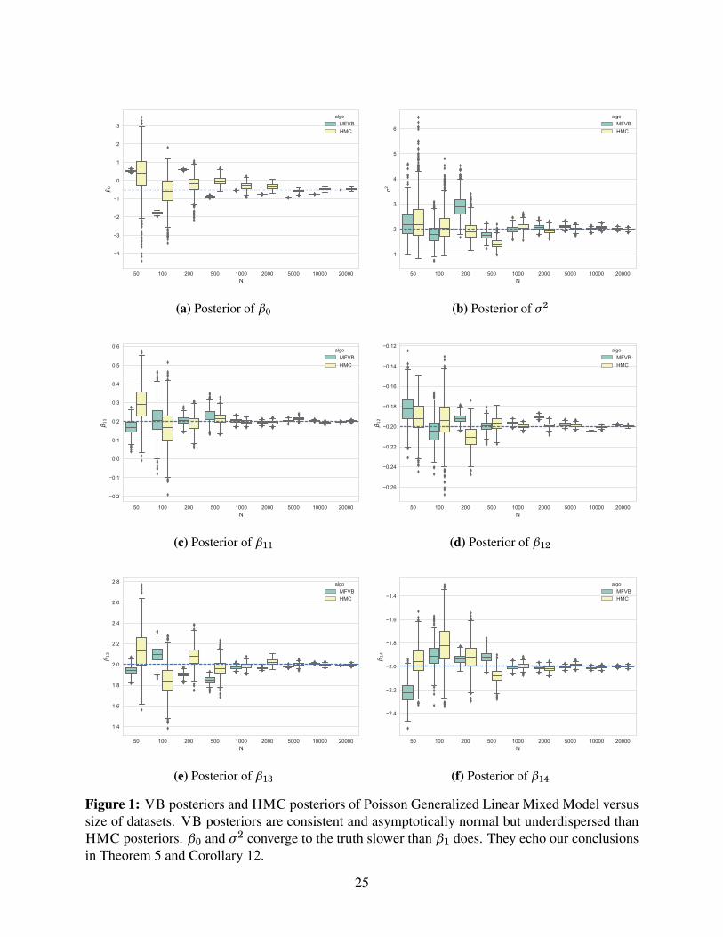
Figure 1 shows the boxplots of VB posteriors for β0,β1, and σ2. All VB posteriors converge totheir corresponding true values as the size of the data set increases. The box plots present ratherfew outliers; the lower fence, the box, and the upper fence are about the same size. This suggestsnormal VB posteriors. This echoes the consistency and asymptotic normality concluded fromTheorem 5. The VB posteriors are underdispersed, compared to the posteriors via HMC. Thisalso echoes our conclusion of underdispersion in Theorem 5 and Lemma 8.

Regarding the convergence rate, VB posteriors of all dimensions of β1 quickly converge to theirtrue value; the VB posteriors center around their true values as long as N ≥ 1000. The convergenceof VB posteriors of slopes for continuous variables (β11,β12) are generally faster than those forbinary ones (β13,β14). The VB posterior of σ2 shares a similarly fast convergence rate. The VBposterior of the intercept β0, however, struggles; it is away from the true value until the data setsize hits N = 20000. This aligns with the convergence rate inferred in Corollary 12,

pmn for β1

andp

m for β0 and σ2.

Computation wise, VB takes orders of magnitude less time than HMC. The performance of VBposteriors is comparable with that from HMC when the sample size is sufficiently large; in thiscase, we need N = 20000.

5.2 Latent Dirichlet Allocation

Latent Dirichlet Allocation (LDA) is a generative statistical model commonly adopted to describeword distributions in documents by latent topics.

Given M documents, each with Nm,m = 1, ..., M words, composing a vocabulary of V words, weassume K latent topics. Consider two sets of latent variables: topic distributions for documentm, (θm)K×1, m = 1, ..., M and word distributions for topic k, (φk)V×1, k = 1, ...,K . The generativeprocess is

θm ∼pθ, m = 1, ..., M,φk ∼pφ, k = 1, ...,K ,

zm, j ∼Mult(θm), j = 1, ..., Nm,m = 1, ..., M,wm, j ∼Mult(φzm, j ), j = 1, ..., Nm,m = 1, ..., M.

The first two rows are assigning priors assigned to the latent variables. wm, j denotes word j ofdocument m and zm, j denotes its assigned topic.

We simulate a data set with V = 100 sized vocabulary and K = 10 latent topics in M = (10, 20,50, 100, 200, 500, 100) documents. Each document has Nm words where Nm

iid∼ Poi(100). Asthe number of documents M grows, the number of document-specific topic vectors θm growswhile the number of topic-specific word vectors φk stays the same. In this sense, we considerθm,m = 1, ..., M as local latent variables and φk,k = 1, ...,K as global latent variables. We areinterested in the VB posteriors of global latent variables φk,k = 1, ...,K here. We generate thedata sets with true values of θ and φ, where they are random draws from θm

iid∼ Dir((1/K)K×1) andφk

iid∼ Dir((1/V )V×1).

24

50 100 200 500 1000 2000 5000 10000 20000N

4

3

2

1

0

1

2

3

0algo

MFVBHMC

(a) Posterior of β0

50 100 200 500 1000 2000 5000 10000 20000N

1

2

3

4

5

6

2

algoMFVBHMC

(b) Posterior of σ2

50 100 200 500 1000 2000 5000 10000 20000N

0.2

0.1

0.0

0.1

0.2

0.3

0.4

0.5

0.6

11

algoMFVBHMC

(c) Posterior of β11

50 100 200 500 1000 2000 5000 10000 20000N

0.26

0.24

0.22

0.20

0.18

0.16

0.14

0.12

12

algoMFVBHMC

(d) Posterior of β12

50 100 200 500 1000 2000 5000 10000 20000N

1.4

1.6

1.8

2.0

2.2

2.4

2.6

2.8

13

algoMFVBHMC

(e) Posterior of β13

50 100 200 500 1000 2000 5000 10000 20000N

2.4

2.2

2.0

1.8

1.6

1.4

14

algoMFVBHMC

(f) Posterior of β14

Figure 1: VB posteriors and HMC posteriors of Poisson Generalized Linear Mixed Model versussize of datasets. VB posteriors are consistent and asymptotically normal but underdispersed thanHMC posteriors. β0 and σ2 converge to the truth slower than β1 does. They echo our conclusionsin Theorem 5 and Corollary 12.

25

10 20 50 100 200 500 1000M

0.2

0.4

0.6

0.8

1.0

KL

(a) Posterior mean KL divergence of theK = 10 topics

10 20 50 100 200 500 1000M

0.2

0.4

0.6

0.8

1.0

1.2

1.4

1.6

KL

algoHMCMFVB

(b) Boxplots of posterior KL divergence of Topic 2

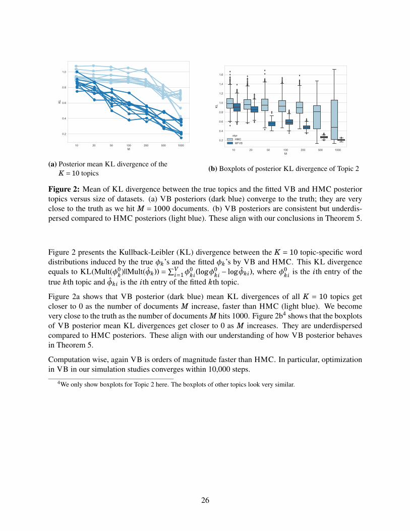
Figure 2: Mean of KL divergence between the true topics and the fitted VB and HMC posteriortopics versus size of datasets. (a) VB posteriors (dark blue) converge to the truth; they are veryclose to the truth as we hit M = 1000 documents. (b) VB posteriors are consistent but underdis-persed compared to HMC posteriors (light blue). These align with our conclusions in Theorem 5.

Figure 2 presents the Kullback-Leibler (KL) divergence between the K = 10 topic-specific worddistributions induced by the true φk’s and the fitted φk’s by VB and HMC. This KL divergenceequals to KL(Mult(φ0

k)||Mult(φk)) = ∑Vi=1φ

0ki(logφ0

ki − log φki), where φ0ki is the ith entry of the

true kth topic and φki is the ith entry of the fitted kth topic.

Figure 2a shows that VB posterior (dark blue) mean KL divergences of all K = 10 topics getcloser to 0 as the number of documents M increase, faster than HMC (light blue). We becomevery close to the truth as the number of documents M hits 1000. Figure 2b4 shows that the boxplotsof VB posterior mean KL divergences get closer to 0 as M increases. They are underdispersedcompared to HMC posteriors. These align with our understanding of how VB posterior behavesin Theorem 5.

Computation wise, again VB is orders of magnitude faster than HMC. In particular, optimizationin VB in our simulation studies converges within 10,000 steps.

4We only show boxplots for Topic 2 here. The boxplots of other topics look very similar.

26

6 Discussion

Variational Bayes (VB) methods are a fast alternative to Markov chain Monte Carlo (MCMC)for posterior inference in Bayesian modeling. However, few theoretical guarantees have beenestablished. This work proves consistency and asymptotic normality for variational Bayes (VB)posteriors. The convergence is in the sense of total variation (TV) distance converging to zero inprobability. In addition, we establish consistency and asymptotic normality of variational Bayesestimate (VBE). The result is frequentist in the sense that we assume a data generating distributiondriven by some fixed nonrandom true value for global latent variables.

These results rest on ideal variational Bayes and its connection to frequentist variational approxi-mations. Thus this work bridges the gap in asymptotic theory between the frequentist variationalapproximation, in particular the variational frequentist estimate (VFE), and variational Bayes. Italso assures us that variational Bayes as a popular approximate inference algorithm bears sometheoretical soundness.

We present our results in the classical VB framework but the results and proof techniques aremore generally applicable. Our results can be easily generalized to more recent developments ofVB beyond Kullback-Leibler (KL) divergence, α-divergence or χ-divergence for example (Li andTurner, 2016; Dieng et al., 2016). They are also applicable to more expressive variational families,as long as they contain the mean field family. We could also allow for model misspecification,as long as the variational loglikelihood Mn(θ ; x) under the misspecified model still enjoys localasymptotic normality.

There are several interesting avenues for future work. The variational Bernstein–von Mises theo-rem developed in this work applies to parametric and semiparametric models. One direction is tostudy the VB posteriors in nonparametric settings. A second direction is to characterize the finite-sample properties of VB posteriors. Finally, we characterized the asymptotics of an optimizationproblem, assuming that we obtain the global optimum. Though our simulations corroborated thetheory, VB optimization typically finds a local optimum. Theoretically characterizing these localoptima requires further study of the optimization loss surface.

Acknowledgements. We thank the associate editor and two anonymous reviewers for theirinsightful comments. We thank Adji Dieng, Christian Naesseth, and Dustin Tran for their valuablefeedback on our manuscript. We also thank Richard Nickl for pointing us to a key reference. Thiswork is supported by ONR N00014-11-1-0651, DARPA PPAML FA8750-14-2-0009, the AlfredP. Sloan Foundation, and the John Simon Guggenheim Foundation.

27

ReferencesAbbe, E. and Sandon, C. (2015). Community detection in general stochastic block models: funda-

mental limits and efficient recovery algorithms. arXiv preprint arXiv:1503.00609.

Alquier, P. and Ridgway, J. (2017). Concentration of tempered posteriors and of their variationalapproximations. arXiv preprint arXiv:1706.09293.

Alquier, P., Ridgway, J., and Chopin, N. (2016). On the properties of variational approximationsof gibbs posteriors. Journal of Machine Learning Research, 17(239):1–41.

Amir-Moez, A. and Johnston, G. (1969). On the product of diagonal elements of a positive matrix.Mathematics Magazine, 42(1):24–26.

Beckenbach, E. F. and Bellman, R. (2012). Inequalities, volume 30. Springer Science & BusinessMedia.

Bernstein, S. N. (1917). Theory of Probability.

Bickel, P., Choi, D., Chang, X., Zhang, H., et al. (2013). Asymptotic normality of maximumlikelihood and its variational approximation for stochastic blockmodels. The Annals of Statistics,41(4):1922–1943.

Bickel, P., Kleijn, B., et al. (2012). The semiparametric Bernstein–von Mises theorem. The Annalsof Statistics, 40(1):206–237.

Bickel, P. J. and Yahav, J. A. (1967). Asymptotically pointwise optimal procedures in sequentialanalysis.

Bishop, C. M. (2006). Pattern recognition. Machine Learning, 128.

Blei, D., Kucukelbir, A., and McAuliffe, J. (2016). Variational inference: A review for statisticians.Journal of the American Statistical Association.

Blei, D. M., Ng, A. Y., and Jordan, M. I. (2003). Latent dirichlet allocation. Journal of MachineLearning Research, 3(Jan):993–1022.

Bontemps, D. et al. (2011). Bernstein–von Mises theorems for gaussian regression with increasingnumber of regressors. The Annals of Statistics, 39(5):2557–2584.

Boucheron, S., Gassiat, E., et al. (2009). A Bernstein–von Mises theorem for discrete probabilitydistributions. Electronic Journal of Statistics, 3:114–148.

Braides, A. (2006). A handbook of Γ-convergence. Handbook of Differential Equations: Station-ary Partial Differential Equations, 3:101–213.

Breslow, N. E. and Clayton, D. G. (1993). Approximate inference in generalized linear mixedmodels. Journal of the American Statistical Association, 88(421):9–25.

Carpenter, B., Gelman, A., Hoffman, M., Lee, D., Goodrich, B., Betancourt, M., Brubaker, M. A.,Guo, J., Li, P., and Riddell, A. (2015). Stan: a probabilistic programming language. Journal ofStatistical Software.

28

Castillo, I. (2012a). Semiparametric Bernstein–von Mises theorem and bias, illustrated with gaus-sian process priors. Sankhya A, 74(2):194–221.

Castillo, I. (2012b). A semiparametric Bernstein–von Mises theorem for gaussian process priors.Probability Theory and Related Fields, 152(1):53–99.

Castillo, I. et al. (2014a). On Bayesian supremum norm contraction rates. The Annals of Statistics,42(5):2058–2091.

Castillo, I. and Nickl, R. (2012). Nonparametric Bernstein–von Mises theorems. arXiv preprintarXiv:1208.3862.

Castillo, I., Nickl, R., et al. (2013). Nonparametric Bernstein–von Mises theorems in gaussianwhite noise. The Annals of Statistics, 41(4):1999–2028.

Castillo, I., Nickl, R., et al. (2014b). On the Bernstein–von Mises phenomenon for nonparametricBayes procedures. The Annals of Statistics, 42(5):1941–1969.

Castillo, I., Rousseau, J., et al. (2015). A Bernstein–von Mises theorem for smooth functionals insemiparametric models. The Annals of Statistics, 43(6):2353–2383.

Celisse, A., Daudin, J.-J., Pierre, L., et al. (2012). Consistency of maximum-likelihood and varia-tional estimators in the stochastic block model. Electronic Journal of Statistics, 6:1847–1899.

Chen, Y.-C., Wang, Y. S., and Erosheva, E. A. (2017). On the use of bootstrap with vari-ational inference: Theory, interpretation, and a two-sample test example. arXiv preprintarXiv:1711.11057.

Cox, D. D. (1993). An analysis of Bayesian inference for nonparametric regression. The Annalsof Statistics, pages 903–923.

Dal Maso, G. (2012). An introduction to Γ-convergence, volume 8. Springer Science & BusinessMedia.

De Blasi, P. and Hjort, N. L. (2009). The Bernstein–von Mises theorem in semiparametric com-peting risks models. Journal of Statistical Planning and Inference, 139(7):2316–2328.

Dempster, A., Laird, N., and Rubin, D. (1977). Maximum likelihood from incomplete data via theEM algorithm. Journal of the Royal Statistical Society, Series B, 39:1–38.

Diaconis, P. and Freedman, D. (1986). On the consistency of Bayes estimates. The Annals ofStatistics, pages 1–26.

Diaconis, P. and Freedman, D. (1997). Consistency of Bayes estimates for nonparametric regres-sion: A review. In Festschrift for Lucien Le Cam, pages 157–165. Springer.

Diaconis, P. W., Freedman, D., et al. (1998). Consistency of Bayes estimates for nonparametricregression: normal theory. Bernoulli, 4(4):411–444.

Dieng, A. B., Tran, D., Ranganath, R., Paisley, J., and Blei, D. M. (2016). Variational inferencevia χ-upper bound minimization. arXiv preprint arXiv:1611.00328.

29

Freedman, D. et al. (1999). Wald lecture: On the Bernstein–von Mises theorem with infinite-dimensional parameters. The Annals of Statistics, 27(4):1119–1141.

Gelfand, A. E. and Smith, A. F. (1990). Sampling-based approaches to calculating marginal den-sities. Journal of the American Statistical Association, 85(410):398–409.

Ghorbani, B., Javadi, H., and Montanari, A. (2018). An instability in variational inference for topicmodels. arXiv preprint arXiv:1802.00568.

Ghosal, S. and van der Vaart, A. (2017). Fundamentals of nonparametric Bayesian inference,volume 44. Cambridge University Press.

Ghosh, J. and Ramamoorthi, R. (2003). Bayesian Nonparametrics. Springer Series in Statistics.Springer.

Giordano, R., Broderick, T., and Jordan, M. I. (2017a). Covariances, robustness, and variationalBayes. arXiv preprint arXiv:1709.02536.

Giordano, R., Liu, R., Varoquaux, N., Jordan, M. I., and Broderick, T. (2017b). Measur-ing cluster stability for Bayesian nonparametrics using the linear bootstrap. arXiv preprintarXiv:1712.01435.

Hall, P., Ormerod, J. T., and Wand, M. (2011a). Theory of gaussian variational approximation fora Poisson mixed model. Statistica Sinica, pages 369–389.

Hall, P., Pham, T., Wand, M. P., Wang, S. S., et al. (2011b). Asymptotic normality and validinference for Gaussian variational approximation. The Annals of Statistics, 39(5):2502–2532.

Hastings, W. (1970). Monte Carlo sampling methods using Markov chains and their applications.Biometrika, 57:97–109.

Hoffman, M., Blei, D., Wang, C., and Paisley, J. (2013). Stochastic variational inference. Journalof Machine Learning Research, 14:1303–1347.

Hoffman, M. D. and Gelman, A. (2014). The No-U-Turn sampler. Journal of Machine LearningResearch, 15(1):1593–1623.

Hofman, J. and Wiggins, C. (2008). Bayesian approach to network modularity. Physical ReviewLetters, 100(25).

James, L. F. et al. (2008). Large sample asymptotics for the two-parameter poisson–dirichletprocess. In Pushing the Limits of Contemporary Statistics: Contributions in Honor of JayantaK. Ghosh, pages 187–199. Institute of Mathematical Statistics.

Jiang, J. (2007). Linear and generalized linear mixed models and their applications. SpringerScience & Business Media.

Johnstone, I. M. (2010). High dimensional Bernstein–von Mises: simple examples. Institute ofMathematical Statistics Collections, 6:87.

Jordan, M. I., Ghahramani, Z., Jaakkola, T. S., and Saul, L. K. (1999). An introduction to varia-tional methods for graphical models. Machine Learning, 37(2):183–233.

30

Kim, Y. (2009). A Bernstein–von Mises theorem for doubly censored data. Statistica Sinica, pages581–595.

Kim, Y. et al. (2006). The Bernstein–von Mises theorem for the proportional hazard model. TheAnnals of Statistics, 34(4):1678–1700.

Kim, Y. and Lee, J. (2004). A Bernstein–von Mises theorem in the nonparametric right-censoringmodel. Annals of statistics, pages 1492–1512.

Kleijn, B., Van der Vaart, A., et al. (2012). The Bernstein–von Mises theorem under misspecifica-tion. Electronic Journal of Statistics, 6:354–381.

Knapik, B. T., van der Vaart, A. W., van Zanten, J. H., et al. (2011). Bayesian inverse problemswith gaussian priors. The Annals of Statistics, 39(5):2626–2657.

Kucukelbir, A., Tran, D., Ranganath, R., Gelman, A., and Blei, D. M. (2016). Automatic differen-tiation variational inference. arXiv preprint arXiv:1603.00788.

Laplace, P. (1809). Memoire sur les integrales definies et leur application aux probabilites, etspecialement a la recherche du milieu qu’il faut choisir entre les resultats des observations.Memoires presentes a l’Academie des Sciences, Paris.

Le Cam, L. (1953). On some asymptotic properties of maximum likelihood estimates and relatedbayes estimates. Univ. Calif. Publ. in Statist., 1:277–330.

Le Cam, L. and Yang, G. L. (2012). Asymptotics in statistics: some basic concepts. SpringerScience & Business Media.

Leahu, H. et al. (2011). On the Bernstein–von Mises phenomenon in the gaussian white noisemodel. Electronic Journal of Statistics, 5:373–404.

Lehmann, E. L. and Casella, G. (2006). Theory of point estimation. Springer Science & BusinessMedia.

Li, Y. and Turner, R. E. (2016). Rényi divergence variational inference. In Advances in NeuralInformation Processing Systems, pages 1073–1081.

Liu, Q. and Wang, D. (2016). Stein variational gradient descent: A general purpose Bayesianinference algorithm. In Advances In Neural Information Processing Systems, pages 2378–2386.

Lu, Y. (2017). On the Bernstein–von Mises theorem for high dimensional nonlinear Bayesianinverse problems. arXiv preprint arXiv:1706.00289.

Lu, Y., Stuart, A. M., and Weber, H. (2016). Gaussian approximations for probability measures onRd. arXiv preprint arXiv:1611.08642.

McCullagh, P. (1984). Generalized linear models. European Journal of Operational Research,16(3):285–292.

McCulloch, C. E. and Neuhaus, J. M. (2001). Generalized linear mixed models. Wiley OnlineLibrary.

31

Mossel, E., Neeman, J., and Sly, A. (2012). Stochastic block models and reconstruction. arXivpreprint arXiv:1202.1499.

Murphy, K. P. (2012). Machine learning: a probabilistic perspective. MIT press.

Murphy, S. A. and Van der Vaart, A. W. (2000). On profile likelihood. Journal of the AmericanStatistical Association, 95(450):449–465.

Ormerod, J. T. and Wand, M. P. (2010). Explaining variational approximations. The AmericanStatistician, 64(2):140–153.

Ormerod, J. T., You, C., and Muller, S. (2014). A variational Bayes approach to variable selection.Technical report, Citeseer.

Panov, M., Spokoiny, V., et al. (2015). Finite sample Bernstein–von Mises theorem for semipara-metric problems. Bayesian Analysis, 10(3):665–710.

Panov, M. E. and Spokoiny, V. G. (2014). Critical dimension in the semiparametric Bernstein–vonMises theorem. Proceedings of the Steklov Institute of Mathematics, 287(1):232–255.

Pati, D., Bhattacharya, A., and Yang, Y. (2017). On statistical optimality of variational Bayes.arXiv preprint arXiv:1712.08983.

Ranganath, R., Tran, D., Altosaar, J., and Blei, D. (2016a). Operator variational inference. InAdvances in Neural Information Processing Systems, pages 496–504.

Ranganath, R., Tran, D., and Blei, D. (2016b). Hierarchical variational models. In InternationalConference on Machine Learning, pages 324–333.

Ray, K. (2014). Adaptive Bernstein–von Mises theorems in gaussian white noise. arXiv preprintarXiv:1407.3397.

Rivoirard, V., Rousseau, J., et al. (2012). Bernstein–von Mises theorem for linear functionals ofthe density. The Annals of Statistics, 40(3):1489–1523.

Robert, C. and Casella, G. (2004). Monte Carlo Statistical Methods. Springer Texts in Statistics.Springer-Verlag, New York, NY.

Roberts, S. J., Husmeier, D., Rezek, I., and Penny, W. (1998). Bayesian approaches to Gaus-sian mixture modeling. IEEE Transactions on Pattern Analysis and Machine Intelligence,20(11):1133–1142.

Sheth, R. and Khardon, R. (2017). Excess risk bounds for the Bayes risk using variational inferencein latent gaussian models. In Advances in Neural Information Processing Systems, pages 5157–5167.

Snijders, T. A. and Nowicki, K. (1997). Estimation and prediction for stochastic blockmodels forgraphs with latent block structure. Journal of Classification, 14(1):75–100.

Spokoiny, V. (2013). Bernstein–von Mises theorem for growing parameter dimension. arXivpreprint arXiv:1302.3430.

32

Tran, D., Blei, D., and Airoldi, E. M. (2015a). Copula variational inference. In Advances in NeuralInformation Processing Systems, pages 3564–3572.

Tran, D., Ranganath, R., and Blei, D. M. (2015b). The variational gaussian process. arXiv preprintarXiv:1511.06499.

Van der Vaart, A. W. (2000). Asymptotic statistics, volume 3. Cambridge University Press.

Von Mises, R. (1931). Wahrscheinlichkeitsrechnung.

Wainwright, M. J. and Jordan, M. I. (2008). Graphical models, exponential families, and varia-tional inference. Foundations and Trends® in Machine Learning, 1(1-2):1–305.

Wang, B. and Titterington, D. (2004). Convergence and asymptotic normality of variationalBayesian approximations for exponential family models with missing values. In Proceedings ofthe 20th Conference on Uncertainty in Artificial Intelligence, pages 577–584. AUAI Press.

Wang, B. and Titterington, D. (2005). Inadequacy of interval estimates corresponding to variationalBayesian approximations. In AISTATS.

Wang, B., Titterington, D., et al. (2006). Convergence properties of a general algorithm for calcu-lating variational Bayesian estimates for a normal mixture model. Bayesian Analysis, 1(3):625–650.

Wang, Y. J. and Wong, G. Y. (1987). Stochastic blockmodels for directed graphs. Journal of theAmerican Statistical Association, 82(397):8–19.

Westling, T. and McCormick, T. H. (2015). Establishing consistency and improving uncertaintyestimates of variational inference through M-estimation. arXiv preprint arXiv:1510.08151.

Yang, Y., Pati, D., and Bhattacharya, A. (2017). α-variational inference with statistical guarantees.arXiv preprint arXiv:1710.03266.

You, C., Ormerod, J. T., and Müller, S. (2014). On variational Bayes estimation and variational in-formation criteria for linear regression models. Australian & New Zealand Journal of Statistics,56(1):73–87.

Zhang, A. Y. and Zhou, H. H. (2017). Theoretical and computational guarantees of mean fieldvariational inference for community detection. arXiv preprint arXiv:1710.11268.

Zhang, F. and Gao, C. (2017). Convergence rates of variational posterior distributions. arXivpreprint arXiv:1712.02519.

33

Appendix

A Proof of Lemma 1

What we need to show here is that our consistent testability assumption implies assumption (2.3)in Kleijn et al. (2012): ∫

θ>Mn

π∗θ(θ | x)dθ

Pθ0→ 0

for every sequence of constants Mn →∞, where θ = δ−1n (θ−θ0).

This is a consequence of a slight generalization of Theorem 3.1 of Kleijn et al. (2012). Thattheorem shows this implication for the iid case with a common

pn-convergence rate for all dimen-

sions of θ. Specifically, they rely on a suitable test sequence under misspecification of uniformexponential power around the true value θ0 to split the posterior measure.

To show this implication in our case, we replace allp

n by δ−1n in the proofs of Theorem 3.1,

Theorem 3.3, Lemma 3.3, Lemma 3.4 of Kleijn et al. (2012). We refer the readers to Kleijn et al.(2012) and omit the proof here.

B Proof of Lemma 2

We first perform a change of variable step regarding the mean field variational family. In light ofLemma 1, we know that the VB ideal degenerates to a point mass at the rate of δ−1

n . We need toassume a variational family that degenerates to points masses at the same rate as the ideal VB pos-terior. This is because if the variational distribution converges to a point mass faster than π(θ | x),then the KL divergence between them will converge to +∞. This makes the KL minimizationmeaningless as n increases. 5

To avoid this pathology, we assume a variational family for the rescaled and re-centered θ, θ :=δ−1

n (θ−µ), for some µ ∈ Θ. This is a centered and scaled transformation of θ, centered to anarbitrary µ. (In contrast, the previous transformation θ was centering θ at the true θ0.) With thistransformation, the variational family is

qθ(θ)= q(µ+δnθ)|det(δn)|, (20)

where q(·) is the original mean field variational family. We will overload the notation in Section 1and write this transformed family as q(θ) and the corresponding family Qd.

5Equation (38) and Equation (108) in the proof exemplify this claim.

34

In this family, for each fixed µ, θ degenerates to a point mass at µ as n goes to infinity. µ is notnecessarily equal to the true value θ0. We allow µ to vary throughout the parameter space Θ so thatQd does not restrict what the distributions degenerate to. Qd only constrains that the variationaldistribution degenerates to some point mass at the rate of δn. This step also does not restrictthe applicability of the theoretical results. In practice, we always have finite samples with fixedn, so assuming a fixed variational family for θ as opposed to θ amounts to a change of variableθ =µ+δnθ.

Next we show consistency of the KL minimizer of the VB ideal.

To show consistency, we need to show that the mass of the KL minimizer

q‡ := argminq(θ)∈Qd

KL(q(θ)||π∗(θ | x))

concentrates near θ0 as n →∞. That is,∫B(θ0,ξn)

q‡(θ)dθPθ0→ 1, (21)

for some ξn → 0 as n →∞. This implies

q‡(θ) d→ δθ0

by the Slutsky’s theorem.

To begin with, we first claim that

limsupn→∞

min KL(q(θ)||π∗(θ | x))≤ M, (22)

for some constant M > 0, and ∫Rd\K

q‡(θ)dθ→ 0, (23)

where K is the compact set assumed in the local asymptotic normality condition.

The first claim says that the limiting minimum KL divergence is upper bounded. The intuition isthat a choice of q(θ) with µ = θ0 would have a finite KL divergence in the limit. This is because(rougly) π∗(θ | x) converges to a normal distribution centered at θ0 with rate δn, so it suffices tohave a q(θ) that shares the same center and the same rate of convergence.

The second claim says that the restriction of q‡(θ) to the compact set K , due to the set compactnessneeded in the local asymptotic normality (LAN) condition, will not affect our conclusion in thelimit. This is because the family of Qd we assume has a shrinking-to-zero scale. In this way, aslong as µ resides within K , q‡(θ) will eventually be very close to its renormalized restriction to thecompact set K , q‡,K (θ), where

q‡,K (θ)= q‡(θ) · Iθ(K)∫q‡(θ) · Iθ(K)dθ

.

35

We will prove these claims at the end.

To show∫

B(θ0,ξn) q‡,K (θ)dθPθ0→ 1, we both upper bound and lower bound this integral. This step

mimicks the Step 2 in the proof of Lemma 3.6 along with Lemma 3.7 in Lu et al. (2016).

We first upper bound the integral using the LAN condition,∫q‡,K (θ)Mn(θ ; x)dθ (24)

=∫

q‡,K (θ)

×[

Mn(θ0 ; x)+δ−1n (θ−θ0)>Vθ0∆n,θ0 −

12

[δ−1n (θ−θ0)]>Vθ0[δ−1

n (θ−θ0)]+ oP (1)]

dθ (25)

≤Mn(θ0 ; x)−C1

d∑i=1

η2

δ2n,ii

∫B(θ0,η)c

q‡,K (θ)dθ+ oP (1), (26)

for large enough n and η << 1 and some constant C1 > 0. The first equality is due to the LANcondition. The second inequality is due to the domination of quadratic term for large n.

Then we lower bound the integral using our first claim. By

limsupn→∞

KL(q‡,K (θ)||π∗(θ | x))≤ M,

we can have ∫q‡,K (θ)Mn(θ ; x)dθ ≥ Mn(θ0 ; x)−M0, (27)

for some large constant M0 > M.

This step is due to a couple of steps of technical calculation and the LAN condition. To show thisimplication, we first rewrite the KL divergence as follows.

KL(q‡,K (θ)||π∗(θ | x)) (28)

=∫

q‡,K (θ) log q‡,K (θ)dθ−∫

q‡,K (θ) logπ∗(θ | x)dθ (29)

=d∑

i=1

∫[δ−1

n,ii q‡,Kh,i (h)] log[δ−1

n,ii q‡,Kh,i (h)]δn,ii dh−

∫q‡,K (θ) logπ∗(θ | x)dθ (30)

= log |det(δn)|−1 +d∑

i=1H(q‡,K

h,i (h))−∫

q‡,K (θ) logπ∗(θ | x)dθ, (31)

where this calculation is due to the form of the Qd family we assume and a change of variableof h = δ−1

n (θ−µ); h is in the same spirit as θ above. Notation wise, µ is the location parameterspecific to q‡,K (θ) and H(qh(h)) denotes the entropy of distribution qh.

We further approximate the last term by the LAN condition.∫q‡,K (θ) logπ∗(θ | x)dθ (32)

36

=∫

q‡,K (θ) logp(θ)exp(Mn(θ ; x))∫p(θ)exp(Mn(θ ; x))dθ

dθ (33)

=∫

q‡,K (θ) log p(θ)dθ+∫

q(θ)Mn(θ ; x)dθ− log∫

p(θ)exp(Mn(θ ; x))dθ (34)

=∫

q‡,K (θ) log p(θ)dθ+∫

q‡,K (θ)Mn(θ ; x)dθ

−[

d2

log(2π)− 12

logdetVθ0 + logdet(δn)+Mn(θ0 ; x)+ log p(θ0)+ oP (1)]

. (35)

This first equality is due to the definition of π∗(θ | x). The second equality is due to∫

q‡,K (θ)dθ = 1.The third equality is due to Laplace approximation and the LAN condition.

Going back to the KL divergence, this approximation gives

KL(q‡,K (θ)||π∗(θ | x)) (36)

= log |det(δn)|−1 +d∑

i=1H(q‡,K

h,i (h))−∫

q‡,K (θ) logπ∗(θ | x)dθ (37)

= log |det(δn)|−1 +d∑

i=1H(q‡,K

h,i (h))−∫

q‡,K (θ) log p(θ)dθ−∫

q‡,K (θ)Mn(θ ; x)dθ

+[

d2

log(2π)− 12

logdetVθ0 + logdet(δn)+Mn(θ0 ; x)+ log p(θ0)+ oP (1)]

(38)

=d∑

i=1H(q‡,K

h,i (h))−∫

q‡,K (θ) log p(θ)dθ−∫

q‡,K (θ)Mn(θ ; x)dθ

+ d2

log(2π)− 12

logdetVθ0 +Mn(θ0 ; x)+ log p(θ0)+ oP (1). (39)

The first equality is exactly Equation (31). The second equality is due to Equation (35). The thirdequality is due to the cancellation of the two logdet(δn) terms. This exemplifies why we assumedthe convergence rate of the Qd family in the first place; we need to avoid the KL divergence goingto infinity.

Bylimsup

n→∞KL(q‡,K (θ)||π∗(θ | x))≤ M,

we have ∫q‡,K (θ)Mn(θ ; x)dθ (40)

≥−M+d∑

i=1H(q‡,K

h,i (h))−∫

q‡,K (θ) log p(θ)dθ

+ d2

log(2π)− 12

logdetVθ0 +Mn(θ0 ; x)+ log p(θ0)+ oP (1) (41)

≥−M0 +Mn(θ0 ; x)+ oP (1) (42)

for some constant M0 > 0. This can be achieved by choosing a large enough M0 to make the last in-equality true. This is doable because all the terms does not change with n except

∫q‡,K (θ) log p(θ)dθ.

And we have limsupn→∞∫

q‡,K (θ) log p(θ)dθ <∞ due to our prior mass condition.

37

Now combining Equation (42) and Equation (26), we have

Mn(θ0 ; x)−C1

d∑i=1

η2

δ2n,ii

∫B(θ0,η)c

q‡,K (θ)dθ+ oP (1)≥−M0 +Mn(θ0 ; x).

This gives ∫B(θ0,η)c

q‡,K (θ)dθ+ oP (1)≤ M0 · (mini δn,ii)2

C2η2 ,

for some constant C2 > 0. The right side of the inequality will go to zero as n goes to infinity if wechoose η=√

M0(mini δn,ii)/C2 → 0. That is, we just showed Equation (21) with ξn = η.

We are now left to show the two claims we made at the beginning.

To show Equation (22), it suffices to show that there exists a choice of q(θ) such that

limsupn→∞

KL(q(θ)||π∗(θ | x))<∞.

We choose q(θ)=∏di=1 N(θi;θ0,i,δ2

n,iivi) for vi > 0, i = 1, ...,d. We thus have

KL(q(θ)||π∗(θ | x)) (43)

=d∑

i=1

12

log(vi)+ d2+d log(2π)−

∫q(θ) log p(θ)dθ−

∫q(θ)Mn(θ ; x)dθ

− 12

logdetVθ0 +Mn(θ0 ; x)+ log p(θ0)+ oP (1) (44)

=d∑

i=1

12

log(vi)+ d2+d log(2π)− log p(θ0)−Mn(θ0 ; x)

− 12

logdetVθ0 +Mn(θ0 ; x)+ log p(θ0)+ oP (1) (45)

=d∑

i=1

12

log(vi)+ d2+d log(2π)− 1

2logdetVθ0 +C6 + oP (1), (46)

for some constant C6 > 0. The finiteness of limsup is due to the last term being bounded in thelimit. The first equality is due to the same calculation as in Equation (45). The third equality isdue to the cancellation of the two Mn(θ0 ; x) terms and the two p(θ0) terms; this renders the wholeterm independent of n. The second equality is due to the limit of q(θ) concentrating around θ0.Specifically, we expand log p(θ) to the second order around θ0,∫

q(θ) log p(θ)dθ (47)

= log p(θ0)+∫

q(θ)[(θ−θ0)(log p(θ0))′+ (θ−θ0)2

2

∫ 1

0(log p(ξθ+ (1−ξ)θ0))′′(1−ξ)2 dξ

]dθ (48)

≤ log p(θ0)+ 12!

maxξ∈[0,1]

{∫q(θ)(θ−θ0)2(log p(ξθ+ (1−ξ)θ0))′′dθ

}(49)

38

≤ log p(θ0)+ Mp√(2π)d det(δ2

n)∏

i vi

∫Rd

|θ|2e(|θ|+|θ0|)2 · e− 12θ

>(δnVδn)−1θ dθ (50)

≤ log p(θ0)+ Mp√(2π)d det(δ2

n)∏

i vi

eθ20

∫Rd

|θ|2e−12θ

>[(δnVδn)−1−2Id]θ (51)

≤ log p(θ0)+C3Mpeθ20 max

d(δ2

n,ii)det(V−1 −2δ2n)−1 (52)

≤ log p(θ0)+C4 maxd

(δ2n,ii) (53)

where maxd(δ2n,ii) → 0 and C3,C4 > 0. The first equality is due to Taylor expansion with integral

form residuals. The second inequality is due to the first order derivative terms equal to zero andtaking the maximum of the second order derivative. The third inequality is due to the prior masscondition where we assume the second derivative of log p(θ) is bounded by Mpe|θ|

2for some

constant Mp > 0. The fourth inequality is pulling eθ20 out of the integral. The fifth inequality is

due to rescaling θ by its covariance matrix and appealing to the mean of a Chi-squared distributionwith d degrees of freedom. The sixth (and last) inequality is due to det(V−1−2δ2

n)−1 > 0 for largeenough n.

We apply the same Taylor expansion argument to the∫

q(θ)Mn(θ ; x)dθ.∫Kn

q(θ)Mn(θ ; x)dθ (54)

=Mn(θ0 ; x)+∫

Kn

q(θ)[δ−1

n (θ−θ0)>Vθ0∆n,θ0 +12

(δ−1n (θ−θ0))>Vθ0δ

−1n (θ−θ0)+ oP (1)

]dθ (55)

≤Mn(θ0 ; x)+ 12

Tr(Vθ0V )+ oP (1) (56)

≤Mn(θ0 ; x)+C6 + oP (1) (57)

where Kn is a compact set. The first equality is due to the LAN condition. The second inequality isdue to q(θ) centered at θ0 with covariance δnVδn. The third inequalities are true for C6 > 0.

For the set outside of this compact set Kn, we consider for a general choice of q distribution,q(θ) =N (θ;θ0 +∆n,θ0 ,δnVθ0δn), of which q(θ) =∏d

i=1 N (θi;θ0,i,δ2n,iivi) we work with is a spe-

cial case. ∫Rd\Kn

q(θ)(log p(θ)+Mn(θ ; x))dθ (58)

≤C7

∫Rd\Kn

N (θ;θ0 +∆n,θ0 ,δnVθ0δn)(log p(θ)+Mn(θ ; x))dθ (59)

≤C8[det(δn)−1 log(det(δn)−1)]∫Rd\Kn

N (θ;∆n,θ0 ,Vθ0) logπ∗(θ | x)det(δn)dθ (60)

≤C9 log(det(δn)−1)]∫Rd\Kn

[π∗(θ | x)+ oP (1)] logπ∗(θ | x),Vθ0)dθ (61)

≤C10 log(det(δn)−1)]∫Rd\Kn

[N (θ;∆n,θ0 ,Vθ0)+ oP (1)] logN (θ;∆n,θ0 ,Vθ0)dθ (62)

≤oP (1) (63)

39

for some C7,C8,C9,C10 > 0. The first inequality is due to q(θ) centered at θ0 and with rate ofconvergence δn. The second inequality is due to a change of variable θ = δ−1

n (θ−θ0). The thirdinequality is due to Lemma 1. The fourth inequality is due to Lemma 1 and Theorem 2 in Pieraand Parada (2009). The fifth inequality is due to a choice of fast enough increasing sequence ofcompact sets Kn.

The lower bound of∫

q(θ)(log p(θ)+Mn(θ ; x))dθ can be derived with exactly the same argument.Our first claim Equation (22) is thus proved.

To show our second claim Equation (23), we first denote B(µ, M) as the largest ball centered at µand contained in the compact set K . We know by the construct of Qd — Qd has a shrinking-to-zero scale — that for each ε> 0, there exists an N such that for all n > N we have

∫||θ−µ||>M q(θ)dθ <

ε. Therefore, we have ∫Rd\K

q‡(θ)dθ ≤∫Rd\B(µ,M)

q‡(θ)dθ ≤ ε.

C Proof of Lemma 3

To show the convergence of optimizers from two minimization problems, we invoke Γ-convergence.It is a classical technique in characterizing variational problems. A major reason is that if two func-tionals Γ−converge, then their minimizer also converge.

We recall the definition of Γ-convergence (Dal Maso, 2012; Braides, 2006).

Definition 14. Let X be a metric space and Fε : X → R a family of functionals indexed by ε> 0.Then the existence of a limiting functional F0, the Γ−limit of Fε, as ε→ 0, relies on two conditions:

1. (liminf inequality) for every x ∈X and for every xε→ x, we have

F0(x)≤ liminfε→0

Fε(xε),

2. (limsup inequality / existence of a recovery sequence) for every x ∈X we can find a sequencexε→ x such that

F0(x)≥ limsupε→0

Fε(xε).

The first condition says that F0 is a lower bound for the sequence Fε, in the sense that F0(x) ≤Fε(xε)+ o(1) whenever xε→ x. Together with the first condition, the second condition implies thatF0(x)= limε→0 Fε(xε), so that the lower bound is sharp.

Γ-convergence is particularly useful for variational problems due to the following fundamental the-orem. Before stating the theorem, we first define equi-coerciveness.

Definition 15. (Equi-coerciveness of functionals) A sequence Fε : X → R is equi-coercise if for allε j → 0 and x j such that Fε j (x j)≤ t there exist a subsequence of j (not relabeled) and a convergingsequence x′j such that Fε j (x

′j)≤ Fε j (x j)+ o(1).

40

Equi-coerciveness of functionals ensures that we can find a precompact minimizing sequence ofFε such that the convergence xε → x can take place. Now we are ready to state the fundamentaltheorem.

Theorem 16. (Fundamental theorem of Γ-convergence) Let X be a metric space. Let (Fε) be anequi- coercise sequence of functions on X . Let F =Γ− limε→0 Fε, then

argminX

F = limε→0

argminX

Fε.

The above theorem implies that if all functions Fε admit a minimizer xε then, up to subsequences,xε converge to a minimum point of F. We remark that the converse is not true; we may haveminimizers of F which are not limits of minimizers of Fε, e.g. Fε(t)= εt2 (Braides, 2006).

In this way, Γ-convergence is convenient to use when we would like to study the asymptotic be-havior of a family of problem Fε through defining a limiting problem F0 which is a ‘good ap-proximation’ such that the minimizers converge: xε → x0, where x0 is a minimizer of F0. Con-versely, we can characterize solutions of a difficult F0 by finding easier approximating Fε (Braides,2006).

We now prove Lemma 3 for the general mean field family. The family is parametric as in Section 1,so we assume it is indexed by some finite dimensional parameter m. We want to show that thefunctionals

Fn(m) := KL(q(θ;m)||π∗(θ | x))

Γ-converge to

F0(m) := KL(q(θ;m)||N (θ;θ0 +δn∆n,θ0 ,δnV−1θ0δn))−∆>

n,θ0Vθ0∆n,θ0

in probability as n → 0. Recall that the mean field family has density

q(θ)=d∏

i=1δ−1

n,ii qh,i(h),

where h = δ−1n (θ−θ0).

We need the following mild technical conditions on Qd.

Following the change-of-variable step detailed in the beginning of Appendix B, we consider themean field variational family with densities q(θ)=∏d

i=1δ−1n,ii qh,i(h), where h = δ−1

n (θ−µ) for someµ ∈Θ.

Assumption 2. We assume the following conditions on qh,i:

1. qh,i, i = 1, ...,d have continuous densities.

2. qh,i, i = 1, ...,d have positive and finite entropies.

3.∫

q′h,i(h)dh <∞, i = 1, ...,d.

41

The last condition ensures that convergence in finite dimensional parameters imlied convergencein TV distance. This is due to a Taylor expansion argument:

KL(q(θ;m)||q(θ;m+δ)) (64)

=∫

q(θ;m) · (log q(θ;m)− log q(θ;m+δ))dθ (65)

=∫

q(θ;m) · (δ · (log q(θ;m))′)dθ+ o(1) (66)

=δ∫

(q(θ;m))′dθ (67)

<ε (68)

The last step is true if Assumption 2 is true for q. We also notice that convergence in KL divergenceimplies convergence in TV distance. Therefore, Assumption 2 implies that convergence in finitedimensional parameter implies convergence in TV distance.

Together with Theorem 16, the Γ-convergence of the two functionals implies mnPθ0→ m0 where mn

is the minimizer of Fn for each n and m0 is the minimizer of F0. This is due to the last term of F0– ∆>

n,θ0Vθ0∆n,θ0 is a constant bounded in Pθ0 probability and independent of m. The convergence

in total variation then follows from Assumption 2 and our argument above.

Lastly, we prove the Γ-convergence of the two functionals for the mean field family.

We first rewrite Fn(m,µ).

Fn(m,µ) := KL(q(θ;m,µ)||π∗(θ | x)) (69)

= log |det(δn)|−1 +d∑

i=1H(qh,i(h;m))−

∫q(θ;m,µ) logπ∗(θ | x))dθ (70)

= log |det(δn)|−1 +d∑

i=1H(qh,i(h;m))−

∫q(θ;m,µ) log p(θ)dθ−

∫q(θ;m,µ)Mn(θ ; x)dθ

+ log∫

p(θ)exp(Mn(θ ; x))dθ (71)

= log |det(δn)|−1 +d∑

i=1H(qh,i(h;m))−

∫q(θ;m,µ) log p(θ)dθ−

∫q(θ;m,µ)Mn(θ ; x)dθ

+[

d2

log(2π)− 12

logdetVθ0 + logdet(δn)+Mn(θ0 ; x)+ log p(θ0)+ oP (1)]

(72)

=d∑

i=1H(qh,i(h;m))−

∫q(θ;m,µ) log p(θ)dθ−

∫q(θ;m,µ)Mn(θ ; x)dθ

+[

d2

log(2π)− 12

logdetVθ0 +Mn(θ0 ; x)+ log p(θ0)+ oP (1)]

(73)

=d∑

i=1H(qh,i(h;m))−

∫q(θ;m,µ)Mn(θ ; x)dθ+ log p(θ0)− log p(µ)

+[

d2

log(2π)− 12

logdetVθ0 +Mn(θ0 ; x)+ oP (1)]

(74)

42

=d∑

i=1H(qh,i(h;m))−

∫q(θ;m,µ)[Mn(θ0 ; x)+δ−1

n (θ−θ0)>Vθ0∆n,θ0 + log p(θ0)− log p(µ)

− 12

(δ−1n (θ−θ0))>Vθ0δ

−1n (θ−θ0)+ oP (1)]dθ−

[d2

log(2π)− 12

logdetVθ0 +Mn(θ0 ; x)+ oP (1)]

(75)

=d∑

i=1H(qh,i(h;m))−

∫δ−1

n (θ−θ0)>Vθ0∆n,θ0 · q(θ;m,µ)dθ

+∫

12

(δ−1n (θ−θ0))>Vθ0δ

−1n (θ−θ0) · q(θ;m,µ)dθ−

[d2

log(2π)− 12

logdetVθ0 + oP (1)]

(76)

The first equality is by the definition of KL divergence. The second equality is by the definition ofthe VB ideal. The third equality is due to the Laplace approximation of the normalizer like we didin Equation (35). The fourth equality is due to the cancellation of the two logdet(δn) terms. Thisagain exemplifies why we assume a fixed variational family on the rescale variable θ. The fifthequality is due to a similar argument as in Equation (45). The sixth equality is due to the LANcondition of Mn(θ ; x). The seventh equality is due to the computation of each term in the integralas an expectation under the distribution q(θ). To extend the restriction to some compact set K tothe whole space Rd in the sixth equality, we employ the same argument as in Equation (46).

We notice that when µ 6= θ0, we will have Fn(m)→∞. On the other hand, we have limsupFn <∞.This echoes our consistency result in Lemma 2.

Now we rewrite F0(m,µ).

KL(q(θ;m,µ)||N (θ;θ0 +δn∆n,θ0 ,δnV−1θ0δn)) (77)

= log |det(δn)|−1 +d∑

i=1H(qh,i(h;m))+

∫q(θ;m,µ) logN (θ;θ0 +δn∆n,θ0 ,δnV−1

θ0δn)dθ (78)

= log |det(δn)|−1 +d∑

i=1H(qh,i(h;m))+ d

2log(2π)− 1

2logdetVθ0 + logdet(δn)

+∫

q(θ;m,µ) · (θ−θ0 −δn∆n,θ0)>δ−1n Vθ0δ

−1n (θ−θ0 −δn∆n,θ0)dθ (79)

=d∑

i=1H(qh,i(h;m))+ d

2log(2π)− 1

2logdetVθ0 +∆>

n,θ0Vθ0∆n,θ0

−∫δ−1

n (θ−θ0)>Vθ0∆n,θ0 · q(θ;m,µ)dθ+∫

12

(δ−1n (θ−θ0))>Vθ0δ

−1n (θ−θ0) · q(θ;m,µ)dθ. (80)

This gives

F0(m,µ)−∆>n,θ0

Vθ0∆n,θ0 (81)

=d∑

i=1H(qh,i(h;m))− d

2log(2π)+ 1

2logdetVθ0

−∫δ−1

n (θ−θ0)>Vθ0∆n,θ0 · q(θ;m,µ)dθ

43

+∫

12

(δ−1n (θ−θ0))>Vθ0δ

−1n (θ−θ0) · q(θ;m,µ)dθ (82)

=+∞· (1− Iµ(θ0))+ [d∑

i=1H(qh,i(h;m))− d

2log(2π)+ 1

2logdetVθ0

−∫δ−1

n (θ−θ0)>Vθ0∆n,θ0 · q(θ;m,µ)dθ

+∫

12

(δ−1n (θ−θ0))>Vθ0δ

−1n (θ−θ0) · q(θ;m,µ)dθ] · Iµ(θ0). (83)

The last step is due to our definition of our variational family q(θ;m,µ) = ∏di=1δ

−1n,ii qh,i(h;m),

where h = δ−1n (θ−µ) for some µ ∈Θ. The last step is true as long as the qh,i distributions are not

point masses at zero. This is ensured by positive entropy in Assumption 2.

Comparing Equation (76) and Equation (83), we can prove the Γ convergence. Let mn → m.When µ 6= θ0, liminfn→∞ Fn(mn,µ) = +∞. The limsup inequality is automatically satisfied.When µ = θ0, we have Fn(m,µ) = F0(m,µ)−∆>

n,θ0Vθ0∆n,θ0 + oP (1). This implies F0(m,µ) ≤

limn→∞ Fn(mn,µ) in Pθ0 probability by the continuity of Fn ensured by Assumption 2.

We then show the existence of a recovery sequence. When µ 6= θ0, F0(m,µ) = +∞. The limsupinequality is automatically satisfied. When µ = θ0, we can simply choose mn = θ0. The limsupinequality is again ensured by F0(m,µ) ≤ limn→∞ Fn(mn,µ) in Pθ0 probability and the continuityof Fn. The Γ-convergence of the F functionals is shown.

We notice that ∆>n,θ0

Vθ0∆n,θ0 does not depend on m or µ so that argminF0 = argminF0 −∆>

n,θ0Vθ0∆n,θ0 . The convergence of the KL minimizers is thus proved.

D Proof of Lemma 4

Notice that the mean field variational families Qd = {q : q(θ)=∏di=1δ

−1n,ii qh,i(h), where h = δ−1

n (θ−µ) for some µ ∈ Θ}, or the Gaussian family {q : q(θ) = N(m,δnΣδn)} can be written in the formof

q(θ)= |detδn|−1qh(δ−1n (θ−µ))

for some µ ∈ Rd, and∫

qh(h)dh = 0. This form is due to a change-of-variable step we detailed inthe beginning of Appendix B.

We first specify the mild technical conditions on Qd.

Assumption 3. We assume the following conditions on qh.

1. If qh is has zero mean, we assume∫

h2 · qh(h)dh <∞ and supz,x |(log p(z, x | θ))′′| ≤ C11 ·qh(θ)−C12 for some C11,C12 > 0; |Mn(θ ; x)′′| ≤ C13 · qh(θ)−C14 for some C13,C14 > 0.

2. If qh has nonzero mean, we assume∫

h · qh(h)dh <∞ and supz,x |(log p(z, x | θ))′| ≤ C11 ·qh(θ)−C12 for some C11,C12 > 0; |Mn(θ ; x)′ ≤ C13| · qh(θ)−C14 for some C13,C14 > 0.

44

The assumption first assumes finite moments for qh so that we can properly apply a Taylor expan-sion argument. The second part of this assumption makes sure the derivative of log p(z, x | θ) doesnot increase faster than the tail decrease of qh(·). For example, if qh(·) is normal, then the secondpart writes supz,x |(log p(z, x | θ))′′| ≤ C15 exp(θ2) for some C15 > 0, and |Mn(θ ; x)′′| ≤ C13 exp(θ2)for some C13 > 0. The latter is satisfied by the LAN condition. This is in general a rather weakcondition. We usually would not expect the derivative of log p(z, x | θ) and Mn(θ ; x) to increasethis fast as θ increases.

Now we are ready to prove the lemma.

We first approximate the profiled evidence lower bound (ELBO), ELBOp(q(θ)).

ELBOp(q(θ)) (84)

:=supq(z)

∫q(θ)

(log

[p(θ)exp

{∫q(z) log

p(x, z|θ)q(z)

dz}]

− log q(θ))dθ, (85)

=∫

q(θ) log p(θ)dθ−∫

q(θ) log q(θ)dθ+supq(z)

∫q(θ)

∫q(z) log

p(x, z|θ)q(z)

dzdθ (86)

=∫

q(θ) log p(θ)dθ−∫

q(θ) log q(θ)dθ

+supq(z)

∫q(θ)[

∫q(z) log

p(x, z|µ)q(z)

dz+ (θ−µ)(∫

q(z) logp(x, z|µ)

q(z)dz

)′=

∫q(θ) log p(θ)dθ−

∫q(θ) log q(θ)dθ+sup

q(z)

∫q(z) log

p(x, z|µ)q(z)

dz

+∫

q(θ)12|θ−µ|2

(∫q(z) log

p(x, z|θ†)q(z)

dz)′′

]dθ (87)

≥∫

q(θ) log p(θ)dθ−∫

q(θ) log q(θ)dθ+supq(z)

∫q(z) log

p(x, z|µ)q(z)

dz

−C15

∫q(θ)

12|θ−µ|2qh(θ)−C12 dθ (88)

=∫

q(θ) log p(θ)dθ−∫

q(θ) log q(θ)dθ+supq(z)

∫q(z) log

p(x, z|µ)q(z)

dz

−C15

∫qh(h)

12|δnh|2qh(µ+δnh)−C12 dh (89)

≥∫

q(θ) log p(θ)dθ−∫

q(θ) log q(θ)dθ+supq(z)

∫q(z) log

p(x, z|µ)q(z)

dz

−C16 mini

(δ2n,ii) (90)

=∫

q(θ) log p(θ)dθ−∫

q(θ) log q(θ)dθ+supq(z)

∫q(z) log

p(x, z|µ)q(z)

dz+ o(1), (91)

for some constant C16 > 0. The first equality is by the definition of ELBOp(q(θ)). The secondequality is rewriting the integrand. The third equality is due to mean value theorem where θ† issome value between µ and θ. (A very similar argument for qh with nonzero means can be madestarting from here, that is expanding only to the first order term.) The fourth equality is due to

45

qh(·) having zero mean. The fifth inequality is due to the second part of Assumption 3. The sixthinequality is due to a change of variable h = δn(θ−µ). The seventh inequality is due to qh(·)residing within exponential family with finite second moment (the first part of Assumption 3). Theeighth equality is due to δn → 0 as n →∞.

We now approximate −KL(q(θ)||π∗(θ|x)) in a similar way.

−KL(q(θ)||π∗(θ|x)) (92)

=∫

q(θ) logp(θ)exp(Mn(θ ; x))

q(θ)dθ (93)

=∫

q(θ)

(log

[p(θ)exp

{supq(z)

∫q(z) log

p(x, z|θ)q(z)

}]− log q(θ)

)dθ (94)

=∫

q(θ) log p(θ)dθ−∫

q(θ) log q(θ)dθ+∫

q(θ)[supq(z)

∫q(z) log

p(x, z|µ)q(z)

dz

+ (θ−µ)

(supq(z)

∫q(z) log

p(x, z|µ)q(z)

dz

)′+ 1

2|θ−µ|2

(supq(z)

∫q(z) log

p(x, z| ˜θ†)q(z)

dz

)′′]dθ (95)

=∫

q(θ) log p(θ)dθ−∫

q(θ) log q(θ)dθ+supq(z)

∫q(z) log

p(x, z|µ)q(z)

dz

+∫

q(θ)12|θ−µ|2

(supq(z)

∫q(z) log

p(x, z| ˜θ†)q(z)

dz

)′′]dθ (96)

≤∫

q(θ) log p(θ)dθ−∫

q(θ) log q(θ)dθ+supq(z)

∫q(z) log

p(x, z|µ)q(z)

dz

+C17

∫q(θ)

12|θ−µ|2qh(θ)−C14 dθ (97)

=∫

q(θ) log p(θ)dθ−∫

q(θ) log q(θ)dθ+supq(z)

∫q(z) log

p(x, z|µ)q(z)

dz

+C17

∫qh(h)

12|δnh|2qh(µ+δnh)−C14 dh (98)

≤∫

q(θ) log p(θ)dθ−∫

q(θ) log q(θ)dθ+supq(z)

∫q(z) log

p(x, z|µ)q(z)

dz+C17 maxi

(δ2n,ii) (99)

=∫

q(θ) log p(θ)dθ−∫

q(θ) log q(θ)dθ+supq(z)

∫q(z) log

p(x, z|µ)q(z)

dz+ o(1) (100)

for some constant C17 > 0. The first equality is by the definition of KL divergence. The secondequality is rewriting the integrand. The third equality is due to mean value theorem where ˜θ† issome value between µ and θ. (A very similar argument for qh with nonzero means can be madestarting from here, that is expanding only to the first order term.) The fourth equality is due toqh(·) having zero mean. The fifth inequality is due to the third part of Assumption 3. The sixthinequality is due to a change of variable h = δn(θ−µ). The seventh inequality is due to qh(·)residing within exponential family with finite second moment (the first part of Assumption 3). Theeighth equality is due to δn → 0 as n →∞.

46

Combining the above two approximation, we have −KL(q(θ)||π∗(θ|x))≤ ELBOp(q(θ))+o(1). Onthe other hand, we know that ELBOp(q(θ))≤−KL(q(θ)||π∗(θ|x)) by definition. We thus concludeELBOp(q(θ))=−KL(q(θ)||π∗(θ|x))+ oP (1).

E Proof of Theorem 5 and Theorem 6

Theorem 5 is a direct consequence of Lemma 2, Lemma 3, and Lemma 4. Lemma 2 and Lemma 3characterizes the consistency and asymptotic normality of the KL minimizer of the VB ideal.Lemma 4 says the VB posterior shares the same asymptotic properties as the VB ideal. All ofthem together give the consistency and asymptotic normality of VB posteriors.

Theorem 6 is a consequence of a slight generalization of Theorem 2.3 of Kleijn et al. (2012). Thetheorem characterizes the consistency and asymptotic normality of the posterior mean estimateunder model specification with a common

pn-convergence rate. We only need to replace all

pn

by δ−1n in their proof to obtain the generalization.

Specifically, we first show that, for any Mn →∞,∫||θ||>Mn

||θ||2q∗(θ)dθPθ0→ 0.

This is ensured by Assumption 3.1.

We then consider three stochastic processes: fix some compact set K and for given M > 0,

t 7→ Zn,M(t)=∫||θ||≤M

(t− θ)2 · q∗θ(θ)dθ, (101)

t 7→Wn,M(t)=∫||θ||≤M

(t− θ)2 ·N (θ;∆n,θ0 ,V−1θ0

)dθ, (102)

t 7→WM(t)=∫||θ||≤M

(t− θ)2 ·N (θ; X ,V−1θ0

)dθ. (103)

We note that θ∗n is the minimizer of t 7→ Zn,∞(t) and∫θ ·argminq∈Qd KL(q(θ)||N (θ ; X ,V−1

θ0))dθ

is the minimizer of t 7→W∞(t).

By supt∈K ,||h||≤M(t− h)2 < ∞, we have Zn,M −Wn,M = oPθ0(1) in `∞(K) by Theorem 5. Since

∆n,θ0d→ X , the continuous mapping theorem implies that Wn,M −WM = oPθ0

(1) in `∞(K). By∫θ · q∗(θ)<∞, we have WM −W∞ = oPθ0

(1) as M →∞. We conclude that there exists a sequenceMn →∞ such that Zn,Mn −W∞ = oPθ0

(1). We also have from above that Zn,Mn −Zn,∞ = oPθ0(1)

in `∞(K). We conclude that Zn,∞ −W∞ = oPθ0(1) in `∞(K). By the continuity and convexity

of the squared loss, we invoke the argmax theorem and conclude that θ∗n converges weakly to∫θ ·argminq∈Qd KL(q(θ)||N (θ ; X ,V−1

θ0))dθ.

47

F Proof of Corollary 7

We prove Lemma 3 for the Gaussian family. We want to show that the functionals

Fn(m,Σ) := KL(N (θ;m,δnΣδn)||π∗(θ | x))

Γ-converge to

F0(m,Σ) := KL(N (θ;m,δnΣδn)||N (θ;θ0 +δn∆n,θ0 ,δnV−1θ0δn))−∆>

n,θ0Vθ0∆n,θ0

in probability as n → 0. We note that this is equivalent to the Γ-convergence of the functionals ofq: KL(q(·)||π∗

θ(· | x)) to KL(q(·)||N (· ;∆n,θ0 ,V−1

θ0)). This is because the second statement is the

same as the first up to a change of variable step from θ to θ.

Together with Theorem 16, this implies mn,ΣnPθ0→ m0,Σ0 where (mn,Σn) is the minimizer of Fn

for each n and (m0,Σ0) is the minimizer of F0. This is due to the last term of F0 – ∆>n,θ0

Vθ0∆n,θ0 isa constant bounded in Pθ0 probability and independent of m,Σ. The convergence in total variationthen follows from Lemma 4.9 of Klartag (2007), which gives an upper bound on TV distancebetween two Gaussian distributions.

Now we prove the Γ-convergence.

We first rewrite Fn(m,Σ).

Fn(m,Σ) (104):=KL(N (θ;m,δnΣδn)||π∗(θ | x)) (105)

=∫

N (θ;m,δnΣδn) logN (θ;m,δnΣδn)dθ−∫

N (θ;m,δnΣδn) logπ∗(θ | x))dθ (106)

=− d2− d

2log(2π)− logdet(δn)− 1

2logdet(Σ)−

∫N (θ;m,δnΣδn) log p(θ)dθ

−∫

N (θ;m,δnΣδn)Mn(θ ; x)dθ+ log∫

p(θ)exp(Mn(θ ; x))dθ (107)

=− d2− d

2log(2π)− logdet(δn)− 1

2logdet(Σ)−

∫N (θ;m,δnΣδn) log p(θ)dθ

−∫

N (θ;m,δnΣδn)Mn(θ ; x)dθ

+[

d2

log(2π)− 12

logdetVθ0 + logdet(δn)+Mn(θ0 ; x)+ log p(θ0)+ oP (1)]

(108)

=− d2− 1

2logdet(Σ)−

∫N (θ;m,δnΣδn) log p(θ)dθ

−∫

N (θ;m,δnΣδn)Mn(θ ; x)dθ+[−1

2logdetVθ0 +Mn(θ0 ; x)+ log p(θ0)+ oP (1)

](109)

=− d2− 1

2logdet(Σ)−

∫N (θ;m,δnΣδn)Mn(θ ; x)dθ

+[−1

2logdetVθ0 +Mn(θ0 ; x)+ oP (1)

](110)

48

=− d2− 1

2logdet(Σ)−

∫N (θ;m,δnΣδn)[Mn(θ0 ; x)+δ−1

n (θ−θ0)>Vθ0∆n,θ0

− 12

(δ−1n (θ−θ0))>Vθ0δ

−1n (θ−θ0)+ oP (1)]dθ−

[12

logdetVθ0 −Mn(θ0 ; x)+ oP (1)]

(111)

=− d2− 1

2logdet(Σ)−δ−1

n (m−θ0)>Vθ0∆n,θ0 +12

(δ−1n (m−θ0))>Vθ0δ

−1n (m−θ0)

+ 12

Tr(Vθ0 ·Σ)− 12

logdetVθ0 + oP (1). (112)

The first equality is by the definition of KL divergence. The second equality is calculating theentropy of multivariate Gaussian distribution. The third equality is due to the Laplace approxima-tion of the normalizer like we did in Equation (35). The fourth equality is due to the cancellationof the two logdet(δn) terms. This again exemplifies why we assume the family to have varianceδnΣδn. The fifth equality is due to a similar argument as in Equation (45). The intuition is thatN (m,δnΣδn) converges to a point mass as n →∞. The sixth equality is due to the LAN condi-tion of Mn(θ ; x). The seventh equality is due to the computation of each term in the integral asan expectation under the Gaussian distribution N (m,δnΣδn). To extend the restriction to somecompact set K to the whole space Rd in the sixth equality, we employ the same argument as inEquation (46).

We notice that when m 6= θ0, we will have Fn(m,Σ)→∞. On the other hand, we have limsupFn <∞. This echoes our consistency result in Lemma 2.

Now we rewrite F0(m,Σ).

KL(N (θ;m,δnΣδn)||N (θ;θ0 +δn∆n,θ0 ,δnV−1θ0δn)) (113)

=− d2+ 1

2Tr(Vθ0 ·Σ)+ (m−θ0 −δn∆n,θ0)>δ−1

n Vθ0δ−1n (m−θ0 −δn∆n,θ0)

− 12

logdet(Σ)− 12

logdetVθ0 (114)

=− d2− 1

2logdet(Σ)−δ−1

n (m−θ0)>Vθ0∆n,θ0 +12

(δ−1n (m−θ0))>Vθ0δ

−1n (m−θ0)

+ 12

Tr(Vθ0 ·Σ)− 12

logdetVθ0 +∆>n,θ0

Vθ0∆n,θ0 . (115)

This gives

F0(m,Σ)−∆>n,θ0

Vθ0∆n,θ0 (116)

=− d2− 1

2logdet(Σ)−δ−1

n (m−θ0)>Vθ0∆n,θ0 +12

(δ−1n (m−θ0))>Vθ0δ

−1n (m−θ0)

+ 12

Tr(Vθ0 ·Σ)− 12

logdetVθ0 (117)

=+∞· (1− Im(θ0))+ [−d2− 1

2logdet(Σ)+ 1

2Tr(Vθ0 ·Σ)− 1

2logdetVθ0] · Im(θ0). (118)

This equality is due to the KL divergence between two multivariate Gaussian distributions.

49

Comparing Equation (112) and Equation (118), we can prove the Γ convergence. Let mn → mand Σn → Σ. When m 6= θ0, liminfn→∞ Fn(mn,Σn) = +∞. The limsup inequality is automati-cally satisfied. When m = θ0, we have Fn(m,Σ) = F0(m,Σ)−∆>

n,θ0Vθ0∆n,θ0 + oP (1). This implies

F0(m,Σ)≤ limn→∞ Fn(mn,Σn) in Pθ0 probability by the continuity of Fn.

We then show the existence of a recovery sequence. When m 6= θ0, F0(m,Σ) = +∞. The limsupinequality is automatically satified. When m = θ0, we can simply choose Σm = Σ and mn = θ0.The limsup inequality is again ensured by F0(m,Σ) ≤ limn→∞ Fn(mn,Σn) in Pθ0 probability andthe continuity of Fn. The Γ-convergence of the F functionals is shown.

We notice that ∆>n,θ0

Vθ0∆n,θ0 does not depend on any of m,Σ so that argminF0 = argminF0 −∆>

n,θ0Vθ0∆n,θ0 . The convergence of the KL minimizers is thus proved.

G Proof of Lemma 8

We first note that

KL(N (·;µ0,Σ0||N (·;µ1,Σ1)) (119)

=12

[Tr(Σ−11 Σ0)+ (µ1 −µ0)>Σ−1

1 (µ1 −µ0)−d+ logdet(Σ1)det(Σ0)

]. (120)

Clearly, the optimal choice of µ0 is µ0 = µ1. Next, we write Σ0 = diag(λ1, ...,λd). The KL diver-gence minimization objective thus becomes

12

[d∑

i=1(Σ−1

1 )iiλi + logdet(Σ1)−d∑

i=1logλi].

Taking its derivative with respect to each λi and setting it to zero, we have

(Σ−11 )ii =λ−1

i .

The optimal Σ0 thus should be diagonal with Σ0,ii = ((Σ−11 )ii)−1 for i = 1,2, ...,d. In this sense,

mean field (factorizable) approximation matches the precision matrix at the mode.

Moreover, by the inequality (Amir-Moez and Johnston, 1969; Beckenbach and Bellman, 2012)

det(Σ−11 )≤∏

i(Σ−1

1 )ii = det(Σ−10 ),

we haveH(Σ−1

0 )= 12

log((2πe)d ·det(Σ0))≤ 12

log((2πe)d ·det(Σ1))=H(Σ1).

50

H Proof of Proposition 10

For simplicity, we prove this proposition for the case when the local latent variables z are dis-crete. The continuous case is easily adapted by replacing the joint probability of (x, z) with themarginal probability of x with z constrained over a neighborhood around zprofile shrinking to apoint mass.

The proof relies on the following inequality:

log p(x, zprofile | θ)≤ Mn(θ ; x)≤ log∫

p(x, z | θ)dz, (121)

where zprofile is the maximum profile likelihood estimate, zprofile := argmaxz p(x, z | θ0). The lowerbound is due to choosing the variational distribution as a point mass at zprofile. The upper bound isdue to the Jensen’s inequality.

Let x be generated by∫

p(x, z | θ = θ0)dz. Condition 1 implies that the posterior of the local latentvariables given the true global latent variables concentrates around zprofile: almost surely underPθ0 ,

p(z | x,θ = θ0) d→ δzprofile .

This convergence result implies

log p(x, zprofile | θ0)= log∫

p(x, z | θ0)dz+ oPθ0(1), (122)

when the local latent variables z are discrete. Hence,

log p(x, zprofile | θ0)= Mn(θ0 ; x)+ oPθ0(1). (123)

Therefore, subtracting Equation (121) by Mn(θ0 ; x) gives

logp(x, zprofile | θ)p(x, zprofile | θ0)

+ oPθ0(1)≤ Mn(θ ; x)−Mn(θ0 ; x)≤ log

∫p(x, z | θ)dz∫p(x, z | θ0)dz

+ oPθ0(1). (124)

The left inequality is due to Equation (123). The right inequality is due to Equation (122) andEquation (123).

Finally recall that, with the two conditions, Theorem 4.2 of Bickel et al. (2012) shows that the logmarginal likelihood has the same LAN expansion as the complete log likelihood in a Hellingerneighborhood around zprofile,

logp(x, zprofile | θ)p(x, zprofile | θ0)

= log∫

p(x, z | θ)dz∫p(x, z | θ0)dz

+ oPθ0(1). (125)

Together with Equation (124), we conclude the variational log likelihood Mn(θ ; x) and the com-plete log likelihood log p(x, z | θ) have the same LAN expansion around θ = θ0.

51

I Proof of Corollary 11

We only need to verify the local asymptotic normality of Ln(µ ; x) here. By Equation (2) of West-ling and McCormick (2015), we know the variational log likelihood writes Ln(µ ; x)=∑

i m(µ ; xi).We Taylor-expand it around the true value µ0:

Ln(µ0 + spn

; x) (126)

=∑i

m(µ0 + spn

; xi) (127)

=∑i

m(µ0 ; xi)+ spn

∑i

Dµm(µ0 ; xi)+ 1n

s>[∑

iD2µm(µ0 ; xi)]s. (128)

Due to X i’s being independent and identically distributed, we have

1pn

∑i

Dµm(µ0 ; xi)=p

n ·∑

i Dµm(µ0 ; xi)n

d→N (0,B(µ))

under Pµ0 , where B(µ) = EPµ0[Dµm(θ ; x)Dµm(µ ; x)>]. The convergence in distribution is due

to central limit theorem. The mean zero here is due to conditions B2, B4, and B5 of Westlingand McCormick (2015) (See point 4 in the first paragraph of Proof of Theorem 2 in Westling andMcCormick (2015) for details.)

By strong law of large numbers, we also have

1n

∑i

D2µm(µ0 ; xi)

Pθ0→ EPθ0[D2

µm(µ0 ; xi)].

This gives the local asymptotic normality, for s in a compact set,

Ln(µ0 + spn

; x)= Ln(µ0 ; x)+ s>ΣY − 12

s>Σs+ oP (1),

whereY ∼N (0, A(µ0)−1B(µ0)A(µ0)−1),

andΣ= A(µ0)= EPθ0

[D2µm(µ0 ; xi)]

is a positive definite matrix.

The consistent testability assumption is satisfied by the existence of consistent estimators. This isdue to Theorem 1 of Westling and McCormick (2015).

The corollary then follows from Theorem 5 and Theorem 6 in Section 3.

52

J Proof of Corollary 12

We first verify the local asymptotic normality of the variational log likelihood:

`(β,σ2) := supµ,λ

`(β,σ2,µ,λ) (129)

=supµ,λ

m∑i=1

n∑j=1

{Yi j(β0+β1 X i j+µi)−exp(β0+β1 X i j+µi+λi /2) − log(Yi j!)}

− m2

log(σ2)+ m2− 1

2σ2

n∑i=1

(µ2i +λi)+ 1

2

m∑i=1

log(λi). (130)

We take the Taylor expansion of the variational log likelihood at the true parameter values β00,β0

1, (σ2)0:

`(β00 +

spm

,β01 +

tpmn

, (σ2)0 + rpm

) (131)

=`(β00,β0

1, (σ2)0)+ spm

∂

∂β0`(β0

0,β01, (σ2)0)+ tp

mn∂

∂β1`(β0

0,β01, (σ2)0)

+ rpm

∂

∂σ2`(β00,β0

1, (σ2)0)+ s2

m∂2

∂β20`(β0

0,β01, (σ2)0)+ t2

mn∂2

∂β21`(β0

0,β01, (σ2)0)

+ r2

m∂2

∂(σ2)2`(β00,β0

1, (σ2)0)+ oP (1). (132)

Denote µi and λi as the optimal µ and λ at the true values (β00,β0

1, (σ2)0). Also write Yi· =∑nj=1 Yi j and Bi = ∑n

j=1 exp(β0 +β1X i j). Let β1, β0, σ2 be the maximizers of the `. Hence,we write Bi = ∑n

j=1 exp(β0 + β1X i j). Finally, the moment generating function of X writes φ(t) =E{exp(tX )}.

The cross terms are zero due to Equation (5.21), Equation (5.29), Equation (5.37), and Equation(5.50) of Hall et al. (2011).

We next compute each of the six derivatives terms.

For the first term ∂∂β0

`(β00,β0

1, (σ2)0), we have

1pm

∂

∂β0`(β0

0,β01, (σ2)0) (133)

= 1pm

m∑i=1

[Yi·−Bi exp(µi + 12λi)] (134)

= 1pm

m∑i=1

[Yi·− Bi exp(µi + 12λi)]− 1p

m(β0 − β0)

m∑i=1

Bi exp(µi + 12λi)

− 1pm

(β1 − β1)m∑

i=1Bi exp(µi + 1

2λi)+ oP (1) (135)

=pm1m

m∑i=1

n∑j=1

((β0 − β0)+ (β1 − β1)X i j)exp(β0 + β1X i j)exp(µi + 12λi)+ oP (1) (136)

53

=pm1m

m∑i=1

n∑j=1

((β1 − β1)(X i j −γ(β01))+U)exp(β0 + β1X i j)exp(µi + 1

2λi)+ oP (1) (137)

=pmU1m

m∑i=1

Bi exp(µi + 12λi)+ oP (1) (138)

=pmU1m

m∑i=1

Bi exp(µi + 12λi)+ oP (1) (139)

d→N (0, (σ2)0)[exp(β00)Eexp(β1X i j +Ui)]+ oP (1) (140)

=N (0, (σ2)0)[exp(β00 −

12

(σ2)0)φ(β01)]. (141)

The first equality is due to differentiation with respect to β0. The second equality is due to Taylorexpansion around the VFE. The third equality is due to Equation (3.5) of Hall et al. (2011). Thefourth equation is due to Equation (5.21) of Hall et al. (2011). The fifth equation is due to Equation(5.1) of Hall et al. (2011). The sixth equation is due to the weak law of law numbers and Slutsky’stheorem together with Equation (3.4), Equation (5.16), and Equation (5.18) of Hall et al. (2011).The seventh equality is due to the equation below Equation (5.80) of Hall et al. (2011).

We then compute the fourth term.

1m

∂2

∂β20`(β0

0,β01, (σ2)0) (142)

= 1m

m∑i=1

Bi exp(µi + 12λi)+ oP (1) (143)

P→exp(β0 − 12

(σ2)0)φ(β01). (144)

This step is due to a similar computation to above. The last step is due to weak law of largenumbers and the equation below Equation (5.80) of Hall et al. (2011).

We now compute the third term.

1pm

∂

∂σ2`(β00,β0

1, (σ2)0) (145)

= 1pm

[− m2(σ2)0 + 1

2{(σ2)0}2m∑

i=1(µ2

i + λi)] (146)

=−pm(

12(σ2)0 )(1− σ2

(σ2)0 ) (147)

= 12{(σ2)0}2

pm(σ2 − (σ2)0) (148)

d→N (0,2{(σ2)0}2)1

2{(σ2)0}2. (149)

The first equality is due to differentiation with respect to σ2. The second equality is due to Equation(5.3) of Hall et al. (2011). The third equality is rearranging the terms. The fourth equation is dueto Equation (3.6) of Hall et al. (2011).

54

We then compute the sixth term.

1m

∂2

∂(σ2)2`(β00,β0

1, (σ2)0) (150)

=[−12

1{(σ2)0}2

+ 1{(σ2)0}3

1m

m∑i=1

(µ2i + λi)] (151)

=[−12

1{(σ2)0}2

+ σ2

{(σ2)0}3]+ oP (1) (152)

P→ 12{(σ2)0}2

. (153)

This is due to a similar computation to above. The last step is due to Equation (3.6) of Hall et al.(2011) and the weak law of large numbers.

We next compute the second term.1pmn

∂

∂β1`(β0

0,β01, (σ2)0) (154)

= 1pmn

m∑i=1

n∑j=1

X i j(Yi j −exp(β00 +β0

1X i j + µi + 12λi)) (155)

= 1pmn

m∑i=1

n∑j=1

X i j(Yi j −exp(β0 + β1X i j + µi + 12λi))

+ (β00 − β0)

1pmn

m∑i=1

n∑j=1

X i j(−exp(β0 + β1X i j + µi + 12λi))

+ (β01 − β1)

1pmn

m∑i=1

n∑j=1

X2i j(−exp(β0 + β1X i j + µi + 1

2λi))+ oP (1) (156)

=pmn1

mn

m∑i=1

n∑j=1

((β00 − β0)+ (β0

1 − β1)X i j)X i j(−exp(β0 + β1X i j + µi + 12λi))

+ oP (1) (157)

=pmn1

mn

m∑i=1

n∑j=1

((β01 − β1)(X i j −γ(β0

1))+U)X i j(−exp(β0 + β1X i j + µi + 12λi))

+ oP (1) (158)d→N (0,τ2)exp(β0

0 −12σ2)φ′′(β0

1). (159)

The first equality is due to differentiation with respect to β1. The second equality is due to Taylorexpansion around VFE. The third equality is due to Equation (3.4) of Hall et al. (2011). The fourthequality is due to Equation (5.16), Equation (5.18), and Equation (5.21) of Hall et al. (2011). Thefifth equation is due to the weak law of law numbers and Slutsky’s theorem together with Equation(3.5) and the equation below Equation (5.80) of Hall et al. (2011).

We lastly compute the fifth term.

1mn

∂2

∂β21`(β0

0,β01, (σ2)0) (160)

55

= 1mn

m∑i=1

n∑j=1

X2i j(exp(β0

0 +β01X i j + µi + 1

2λi)) (161)

= 1mn

m∑i=1

n∑j=1

X2i j(exp(β0

0 +β01X i j +Ui)) (162)

P→exp(β00 −

12σ2)φ′′(β0

1). (163)

This is due to a similar computation to above. The last step is due to the weak law of largenumbers.

The calculation above gives the full local asymptotic expansion of `(β0,β1,σ2).

The consistent testability assumption is satisfied by the existence of consistent estimators. This isdue to Theorem 3.1 of Hall et al. (2011). The corollary then follows directly from Theorem 5 andTheorem 6 in Section 3.

K Proof of Corollary 13

We verify the local asymptotic normality of the variational log likelihoodMn(θ ; A)= supq(z)∈QK

∫q(z) log p(A,z | ν,ω)

q(z) dz, where θ = (ν,ω).

We first notice that, for any (A, Z) pair,

log p(A, Z | θ)≤ Mn(θ ; A)≤ log∫

p(A, z | θ)dz. (164)

The lower bound is due to choosing the variational distribution as a point mass at z. The upperbound is due to the Jensen’s inequality.

From now on, assume (A, Z) is generated by θ0. Lemma 3 of Bickel et al. (2013) shows that

log p(A, Z | θ0)= log∫

p(A, z | θ0)dz+ oP (1), (165)

Together with the above sandwich inequality, this result gives us

log p(A, Z | θ0)= Mn(θ0 ; A)+ oPθ0(1). (166)

Theorem 3 of Bickel et al. (2013) says that, up to label switching,

Mn(θ ; A)− log∫

p(A, z | θ0)dz = logff0

(A, Z,θ)+ oP (1). (167)

Together with Equation (166), the above equality implies

Mn(θ ; A)−Mn(θ0 ; A)= logff0

(A, Z,θ)+ oP (1). (168)

56

Finally, Lemma 2 of Bickel et al. (2013) shows that

logff0

(A, Z,ν0 + t√n2ρn

,ω0 + spn

)= s>Y1 + t>Y2 − 12

s>Σ1s− 12

t>Σ2t+ oP (1), (169)

where Σ1,Σ2 are functions of ω0 and ν0, and Y1,Y2 are asymptotically normal distributed withzero mean and covariances Σ1,Σ2. Therefore, we have the LAN expansion for the variational loglikelihood Mn(θ ; A):

Mn(θ ; A) := supq(z)∈QK

∫q(z) log

p(A, z | ν0 + tpn2ρn

,ω0 + spn )

q(z)dz

= supq(z)∈QK

∫q(z) log

p(A, z | ν0,ω0)q(z)

dz+ s>Y1 + t>Y2 − 12

s>Σ1s− 12

t>Σ2t+ oP (1), (170)

for (ν0,ω0) ∈T for compact T with ρn = 1nE(degree of each node).

57

ReferencesAmir-Moez, A. and Johnston, G. (1969). On the product of diagonal elements of a positive matrix.

Mathematics Magazine, 42(1):24–26.

Beckenbach, E. F. and Bellman, R. (2012). Inequalities, volume 30. Springer Science & BusinessMedia.

Bickel, P., Choi, D., Chang, X., Zhang, H., et al. (2013). Asymptotic normality of maximumlikelihood and its variational approximation for stochastic blockmodels. The Annals of Statistics,41(4):1922–1943.

Bickel, P., Kleijn, B., et al. (2012). The semiparametric Bernstein–von Mises theorem. The Annalsof Statistics, 40(1):206–237.

Braides, A. (2006). A handbook of Γ-convergence. Handbook of Differential Equations: Station-ary Partial Differential Equations, 3:101–213.

Dal Maso, G. (2012). An introduction to Γ-convergence, volume 8. Springer Science & BusinessMedia.

Hall, P., Pham, T., Wand, M. P., Wang, S. S., et al. (2011). Asymptotic normality and validinference for Gaussian variational approximation. The Annals of Statistics, 39(5):2502–2532.

Klartag, B. (2007). A central limit theorem for convex sets. Inventiones Mathematicae, 168(1):91–131.

Kleijn, B., Van der Vaart, A., et al. (2012). The Bernstein–von Mises theorem under misspecifica-tion. Electronic Journal of Statistics, 6:354–381.

Lu, Y., Stuart, A. M., and Weber, H. (2016). Gaussian approximations for probability measures onRd. arXiv preprint arXiv:1611.08642.

Piera, F. J. and Parada, P. (2009). On convergence properties of Shannon entropy. Problems ofInformation Transmission, 45(2):75–94.

Westling, T. and McCormick, T. H. (2015). Establishing consistency and improving uncertaintyestimates of variational inference through M-estimation. arXiv preprint arXiv:1510.08151.

58