FREQUENCY RESPONSE APPROXIMATION METHODS …
134
FREQUENCY RESPONSE APPROXIMATION METHODS OF THE DISSIPATIVE MODEL OF FLUID TRANSMISSION LINES by JOHN D. KING Presented to the Faculty of the Graduate School of The University of Texas at Arlington in Partial Fulfillment of the Requirements for the Degree of MASTER OF SCIENCE IN MECHANICAL ENGINEERING THE UNIVERSITY OF TEXAS AT ARLINGTON May 2006
Transcript of FREQUENCY RESPONSE APPROXIMATION METHODS …

FREQUENCY RESPONSE APPROXIMATION METHODS
OF THE DISSIPATIVE MODEL OF FLUID
TRANSMISSION LINES
by
JOHN D. KING
Presented to the Faculty of the Graduate School of
The University of Texas at Arlington in Partial Fulfillment
of the Requirements
for the Degree of
MASTER OF SCIENCE IN MECHANICAL ENGINEERING
THE UNIVERSITY OF TEXAS AT ARLINGTON
May 2006

Copyright © by John D. King 2006
All Rights Reserved

To my wife Lilia
and my daughter Emily

iv
ACKNOWLEDGEMENTS
I want to thank Dr. Hullender for inspiring me in my decision to research fluid
line dynamics while attending his course in Dynamic Systems Modeling. Dr. Hullender
introduced the dissipative model of a fluid transmission and discussed the thesis by
Tom Wongputorn, �Time Domain Simulation of Systems with Fluid Transmission
Lines�. This was the beginning for me to a much deeper understanding of modeling
systems beyond the simple lump parameter models I have studied previously.
I also want to recognize Tom Wongputorn for his application of the Gauss �
Newton method and the standard he set for this research. It was personally very
challenging for me to attempt to build on his work.
I am very grateful to Dr. Nomura who provided me with the mathematical tools
to tackle this research and also sparked my interest in continuum mechanics and the
Navier-Stokes equations. I really enjoyed attending his courses.
In general I want to thank all the professors that I have studied under at The
University of Texas at Arlington. Each one has greatly helped me to be a much better
engineer.
Finally, I want to express my very special gratitude to my wife Lilia who has
supported me through my work.
March 20, 2006
v
ABSTRACT
FREQUENCY RESPONSE APPROXIMATION METHODS
OF THE DISSIPATIVE MODEL OF FLUID
TRANSMISSION LINES
Publication No. ______
John D. King, M.S.
The University of Texas at Arlington, 2006
Supervising Professor: David A. Hullender
This thesis introduces an accurate and efficient method of obtaining a linear
approximation for a nonlinear model of a complete fluid transmission line system using
Matlab® Signal Processing Toolbox and Symbolic Math Toolbox programs. This
technique is then packaged in a Graphical User Interface program to streamline the
process of analyzing a total system.
The nonlinear model applied in this thesis is called the dissipative model and is
also referred to as the �exact� model, because it�s derivation uses all of the Navier-
Stokes equations as well as the equations of state. It has been studied and tested against
real data and is recognized as the most accurate of all the known models.

vi
Other modeling approaches are discussed in this work to illustrate the
completeness of the dissipative model. The modal technique introduced in this thesis is
inspired by the modal approximation method that is based on truncating the infinite
series representation of the dissipative model. This modal approximation method is
covered in depth in this document.
The method of approximating the frequency response of a fluid transmission
line with a rational polynomial transfer function using the Matlab® �invfreqs� least
squares curve fitting algorithm has already been introduced. This work improves the
technique by proving that an accurate result can be obtained by matching the mode with
the resonant frequency, adding one additional order to the characteristic equation, and
then normalizing the result by dividing the approximated transfer function by the steady
state gain. It also improves the technique by applying the �invfreqs� command to a total
system rather than just the one line. The result is that the order of a linear transfer
function for a total fluid transmission line system can be greatly reduced.

vii
TABLE OF CONTENTS
ACKNOWLEDGEMENTS...................................................................................... iv
ABSTRACT ............................................................................................................ v
LIST OF ILLUSTRATIONS.................................................................................... xi
LIST OF TABLES ...................................................................................................xiv
NOMENCLATURE................................................................................................. xv
Chapter
1. INTRODUCTION............................................................................................... 1
1.1 System Modeling Background ..................................................................... 1
1.2 Fluid Transmission Line Modeling History.................................................. 2
1.3 Rational Polynomial Approximations .......................................................... 3
2. FLUID TRANSMISSION LINE MODELING.................................................... 5
2.1 Modeling Overview..................................................................................... 5
2.2 Lumped Parameter Line Models .................................................................. 5
2.3 Distributed Parameter Line Models.............................................................. 10
2.3.1 Lossless Line Model ........................................................................... 13
2.3.2 Linear Friction Model ......................................................................... 14
2.3.3 Viscous Line Model ............................................................................ 16
2.3.4 Dissipative Transmission Line Model ................................................. 17

viii
2.4 Normalized Parameters................................................................................ 18
2.5 Transmission Line Model Comparison......................................................... 21
2.5.1 Lumped Parameter Model ................................................................... 22
2.5.2 Distributed Parameter Models ............................................................. 25
2.5.2.1 Lossless Line Model................................................................ 25
2.5.2.2 Linear Friction Model.............................................................. 25
2.5.2.3 Viscous Model ........................................................................ 26
2.5.2.4 Dissipative Model.................................................................... 26
3. MODAL APPROXIMATION APPROACH ....................................................... 28
3.1 Model Overview.......................................................................................... 28
3.2 Model Derivation......................................................................................... 30
3.2.1 Modal Approximation of 1/cosh Γ....................................................... 32
3.2.2 Modal Approximation of Ζc sinh Γ/cosh Γ........................................... 34
3.2.3 Modal Approximation of sinh Γ / Ζc cosh Γ ......................................... 38
3.3 Modal Approximation Residue Coefficient Tables....................................... 44
3.4 Modal Approximation of a Blocked Hydraulic Line..................................... 48
4. FREQUENCY RESPONSE CURVE FITTING................................................... 54
4.1 Least Squares Method for Linear Curve Fitting............................................ 54
4.2 Nonlinear Least Squares Overview .............................................................. 55
4.2.1 Newton�s Iterative Method.................................................................. 55
4.2.2 Newton�s Method in Optimization ...................................................... 56
4.2.3 The Gauss-Newton Method................................................................. 56

ix
4.3 Approximation of the Dissipative Model Using Gauss-Newton Method....... 57
4.3.1 Levi�s Algorithm................................................................................. 58
4.3.2 Iterative Algorithm to Estimate θ ........................................................ 60
5. APPLICATION OF MATLAB® FUNCTIONS TO OBTAIN A FINITE ORDER TRANSFER FUNCTION OF A TOTAL FLUID TRANSMISSION LINE SYSTEM ..................................................................... 63
5.1 Total Fluid Transmission Line System......................................................... 63
5.2 Application of Matlab® Symbolic Toolbox Commands to Model a Fluid Transmission Line ....................................................................................... 63
5.2.1 Frequency and Time Response of Lumped Model............................... 64
5.2.2 Frequency and Time Response of the Dissipative Model..................... 69
5.3 Application of Matlab® Symbolic Toolbox Commands to Model a Total Fluid Transmission Line System.................................................................. 83 5.4 Application of Matlab® Matrix Commands to Model a Total Fluid Transmission Line System........................................................................... 88
5.5 Application of Matlab® Graphical User Interface to Produce the Fluid Transmission System Analyzer .................................................................... 89
5.6 Fluid Transmission System Analyzer Frequency Selection Application ....... 97
6. SUMMARY OF RESEARCH AND RECOMMENDATION FOR FUTURE STUDY............................................................................................................... 99
6.1 Summary of Research ................................................................................ 99
6.2 Recommendation for Future Study.............................................................100
Appendix
A. MODEL COMPARISON PROGRAM ...............................................................101
B. TRUNCATED PRODUCT SERIES MODAL APPROXIMATION PROGRAM......................................................................................................... 104

x
C. �INVFREQS� MODAL APPROXIMATION COMPARISON PROGRAM........................................................................................................110
REFERENCES ........................................................................................................114
BIOGRAPHICAL STATEMENT ............................................................................117

xi
LIST OF ILLUSTRATIONS
Figure Page
2.1 Basic lumped parameter model ..................................................................... 6
2.2 Two element lumped parameter model.......................................................... 7
2.3 Magnitude and phase frequency response plots of a transmission line modeled with single element lumped parameters.................................... 8
2.4 Magnitude and phase frequency response plots of a transmission line modeled with two element lumped parameters .............................................. 9
2.5 Distributed parameter model ......................................................................... 11
2.6 Frequency magnitude response of a blocked hydraulic line using the dissipative model .......................................................................................... 20
2.7 Frequency phase response of a blocked hydraulic line using the dissipative model .......................................................................................... 21
2.8 Blocked transmission line illustration............................................................ 21
2.9 Frequency magnitude response of common fluid transmission line models .......................................................................................................... 27
3.1 Hydraulic log splitter .................................................................................... 28
3.2 Log-log plot of natural frequency of a hydraulic line as a function of the dimensionless root index..................................................................... 49
3.3 Log-log plot of natural frequency of a hydraulic line as a function of the dimensionless root index............................................................................... 50
3.4 Log-log plot of residue coefficient, (-1)i+1(1-2i)ai of a hydraulic line as a function of the dimensionless root index ................................................ 51
3.5 Log-log plot of residue coefficient, (-1)i+1(1-2i)bi of a hydraulic line as a function of the dimensionless root index ................................................ 52

xii
3.6 Frequency response of modal approximations ............................................... 53 4.1 First approximation using tangent line x-intercept......................................... 55
5.1 Hydraulic brake valve schematic (Mico) ....................................................... 63
5.2 Frequency response plot of lumped parameter model .................................... 68
5.3 Time domain step input response plot of lumped parameter model................ 68
5.4 Frequency magnitude response of dissipative model ..................................... 72
5.5 Frequency response phase plot of dissipative model...................................... 73
5.6 Determination of required number of modes ................................................. 74
5.7 Frequency magnitude response of approximation without fit-error weighting...................................................................................................... 76
5.8 Frequency magnitude response of approximation with fit-error weighting...................................................................................................... 77
5.9 Frequency magnitude response of approximation with normalized gain............................................................................................................... 78
5.10 Frequency response of approximation with normalized gain for the first five modes ........................................................................................... 79
5.11 Frequency magnitude response of approximation using additional order for each mode .................................................................................... 80 5.12 Frequency phase response of approximation using additional order for each mode .................................................................................... 81 5.13 Step input response of modal approximations using �invfreqs� .................... 81
5.14 Impulse input response of modal approximations using �invfreqs�............... 82
5.15 Multiple line system with capacitive and resistive elements ........................ 83
5.16 Frequency response plots for seven line brake system................................. 85
5.17 Frequency response modal approximation plots for seven line brake system............................................................................................... 86

xiii
5.18 Step response modal approximation plot for seven line brake system .......... 87
5.19 Impulse response modal approximation plot for seven line brake system......................................................................................................... 87
5.20 GUI opening screen shot ............................................................................. 89
5.21 GUI material constants section.................................................................... 90
5.22 GUI model properties section...................................................................... 90
5.23 GUI model diagram section ........................................................................ 91
5.24 GUI line lengths section.............................................................................. 91
5.25 GUI line lengths section.............................................................................. 91
5.26 GUI system solution section before analysis ............................................... 92
5.27 GUI system solution section after analysis .................................................. 93
5.28 GUI frequency response comparison output ................................................ 94
5.29 GUI complete screen shot ........................................................................... 95
5.30 GUI layout editor screen shot...................................................................... 96
5.31 GUI files..................................................................................................... 96
5.32 Failure of frequency determination algorithm.............................................. 97
5.33 Accurate approximation using frequency override....................................... 98

xiv
LIST OF TABLES
Table Page
3.1 Residue Coefficients for Air (Pneumatic Transmission Lines) ..................... 44
3.2 Residue Coefficients for Liquid (Hydraulic Transmission Lines) ................. 46
3.3 Residue Coefficients for the Real Poles of Z0 / sinh Γ and Z0 cosh Γ / sinh Γ .................................................................................. 47
3.4 Residue Coefficients for the Real Poles of 1 / Z0 sinh Γ and cosh Γ / Z0 sinh Γ .................................................................................. 48

xv
NOMENCLATURE
A cross sectional area of fluid transmission line )(sA denominator of linear rational polynomial transfer function
maa 21 ,,K numerator polynomial coefficients for the propagation operator Γ
cici ba , normalized numerator coefficients for the modal approximation of cosh Γ
zizi ba , normalized numerator coefficients for the modal approximation of Zcsinh Γ/ Z0cosh Γ
sisi ba , normalized numerator coefficients for the modal approximation of Z0sinh Γ/ Zccosh Γ
i,0α ith zero of the zero-order Bessel function i,1α ith zero of the first-order Bessel function
)(sB numerator of linear rational polynomial transfer function
mbb 21 ,,K denominator polynomial coefficients for the propagation operator Γ
eβ equivalent bulk modulus
sβ secant bulk modulus
Tβ tangent bulk modulus B Bessel function ration applied in the viscous line model
rB Bessel function ratio applied in the dissipative line model
σrB Bessel function ratio with Prandtl number applied in the dissipative line model
222 ,, +mcc K numerator polynomial coefficients used in development of cosh Γ pc specific heat at constant pressure vc specific heat at constant volume
0c speed of sound (m/s) = ρβe
1C cosh Γ/Zc sinh Γ 2C 1/Ζc sinh Γ 3C sinh Γ/ Ζc cosh Γ 4C 1/cosh Γ 5C Zc cosh Γ/sinh Γ 6C Ζc/sinh Γ 7C Zc sinh Γ/cosh Γ
PC lumped capacitance of fluid line = V/βe
d fluid transmission line diameter nD dissipative number = ωv/ωc = νL/c0r2

xvi
)(se error function E error function
nfff ,..., 21 experimental data points used in the development of nonlinear
least squares curve fitting technique )(),...(),( 21 nxfxfxf
set of functions used in the development of nonlinear least squares curve fitting technique
F linear friction coefficient = 8ωv γ specific heat ratio, vp cc / Γ propagation operator
)(sH linear rational polynomial transfer function i second order mode number j 1−
0J zeroth order Bessel function of the first kind 1J first order Bessel function of the first kind fJ Jacobian of a set of functions 0k normalized real term for the real pole of Ζ0 sinh Γ/Zc cosh Γ cλ dimensionless root index for mode i, = ( i - 1/2)/Dn sλ dimensionless root index for mode i, = i/Dn
L lumped inertance = ρl/A n number of second order modes θ parameter vector ρ fluid density
0ρ fluid density at t = 0
kppp L,, 21 parameter of functions f(x1), f(x2),� f(xn) used in the development
of nonlinear least squares curve fitting technique 0P pressure at t = 0
P& time derivative of pressure inP input pressure outP output pressure RP pressure after input valve resistance
Q& time derivative of fluid flow rate inQ input fluid flow rate outQ output fluid flow rate
),( sxQ fluid flow rate variable r line radius R lumped resistance = 128νρl/πd4 s Laplace operator s normalized Laplace operator = sr/ν = s/ωv σ Prandtl number t time T temperature

xvii
oT time average of temperature u fluid velocity component in x-direction u average fluid velocity component in x-direction v fluid velocity component in y-direction V volume ν kinematic viscosity ω frequency (rad/sec)
cω characteristic frequency = c0/L vω viscous frequency = ν/r2
niω normalized natural frequency of ith second order mode iζ damping ratio of ith second order mode cΖ characteristic impedance = 0Ζ line impedance constant = ρ0c0/πr2

1
CHAPTER 1
INTRODUCTION
1.1 System Modeling Background
Engineers want to predict the performance of a system before spending the time
and capital to produce one that may not function as required. Models are produced to
simulate the actual system and modifications are made to the design based on the
performance of the model. The most convenient way to simulate a system is to produce
a quantitative mathematical model. The performance of a system can often be very
accurately predicted using a mathematical model that quantifies all the measurable
dynamic behavior. Depending on the accuracy required these models can be very
simple to extremely complex.
The simplest models are composed linear differential equations containing very
generalized or �lumped� coefficients representing the system�s physical parameters.
Circuit theory is an example of this modeling approach and is quite adequate to obtain
an accurate output for a small electric circuit operating at low frequencies, but not for a
very long electrical transmission line or a circuit operating at very high frequencies.
Fluid systems likewise, can be modeled with the �same� equations, but the accuracy
limited. The model that an engineer uses has to represent all the dynamics that can have
a measurable effect on the result [1/2].

2
1.2 Fluid Transmission Line Modeling History
Fluid and electrical transmission line dynamics have been studied extensively
since their wide span application in the 20th century. Heaviside is credited with the
formulation of transmission line theory for electrical lines in 1887, and his equations are
referred to as the telegrapher�s equations. In contrast to circuit theory, Heaviside�s
equations are based on distributing the parameters of inductance and resistance along
the length of the line. Electrical transmission line theory is derived from the Maxwell�s
equations which are nonlinear partial differential equations. He also proved that an
electrical transmission line can be modeled using just two functions, the propagation
operator Γ and the characteristic impedance Ζ0 [3].
A fluid transmission line system, like a long electrical transmission line, also
needs to be modeled with distributed parameters to accurately quantify the dynamic
behavior. The approach is very similar to electrical transmission line theory, but fluid
transmission line theory is derived from the Navier-Stokes equations which are the
foundational equations of fluid mechanics [4]. These equations obey the basic laws of
conservation of momentum, mass, and energy:
1.) Momentum: The acceleration of fluid particles.
2.) Continuity: The conservation of mass.
3.) Energy: The dissipation of heat.
Since the Navier-Stokes equations do not cover the issue of compressibility whether it
be a gas or a liquid, an additional equation needs to be included in the total solution:
4.) State: The influence of the compressibility of the fluid.

3
Iberall [5] was the first to produce a solution that included viscous friction and
heat transfer effects. Gerlach [6] produced the first exact first order or classical model
solution. From this work researchers have developed several distributed parameter
models which is documented by Goodson and Leonard [7]. The dissipative model is
considered to be the most accurate [8].
1.3 Rational Polynomial Approximations
The major obstacle to the distributed parameter model is that it is nonlinear and
not in the form of a finite order rational polynomial familiar in classical modeling and
control theory. This is a problem because the resulting transfer function cannot be
transformed to the time domain using inverse Laplace transform techniques. To exactly
represent a distributed parameter model in rational polynomial form would require an
infinite order transfer function, because the frequency response of an exact solution
oscillates to infinity. It is important to note that all real systems are distributed
parameter and a finite order rational polynomial transfer function is simply an
approximation. The goal in systems modeling is to have a transfer function
approximation of the order that covers the required frequency range of operation [9].
Model Order Reduction is a branch of dynamic systems modeling research that
seeks to simply or reduce the complexity of a system model without losing measurable
output behavior [10]. The distributed parameter model is an infinite order
representation of a system, and researchers have sought for methods to approximate it
with a finite order model. Brown [11/12] was the first to approximate Iberall�s solution
in the Laplace domain to obtain a step and impulse time domain response. D'Souza and

4
Oldenburger [13] further developed Brown�s approach to include the effects of line
vibration. Hullender and Healey [14] developed a rational polynomial approximation
by obtaining a Tailor�s series expansion of the dissipative solution based on the mode
number. Hullender and Hsue [15] applied the modal approximation approach to the
seven unique solutions of the dissipative model. Hullender and Woods [16] applied the
modal approximation method to the development of a minimum-order state-space
model. Nursilo [17] introduced an approach to correct modal approximations at zero
frequency. Wongputorn [18] introduced an approach by applying a least-squares curve
fitting algorithm in Matlab® to the frequency response of the dissipative model.

5
CHAPTER 2
FLUID TRANSMISSION LINE MODELING 2.1 Modeling Overview
Each of the commonly accepted fluid transmission line models are developed
and compared in this chapter in order to illustrate the importance of having a model that
simulates all the dynamics and also the importance of minimizing the model to the
frequency of operation.
2.2 Lumped Parameter Line Models
The simplest mathematical model of a fluid transmission line is the lumped
parameter model. In this model the three physical parameters, resistance, inertance, and
capacitance are assumed to be located in one or more discrete locations along the fluid
transmission line. This model is constructed with a system of linear ordinary
differential equations (ODEs). This model is useful since it can be integrated into a
larger mechanical system of lumped parameter components to produce a rational
polynomial transfer function. The inverse Laplace transform can then be applied to this
result to obtain the time domain response of the system.

6
Figure 2.1 Basic lumped parameter model
The equations that define this model are as follows:
inRin QRPP =− (2.1)
inoutRQLPP &=− (2.2)
outpoutin PCQQ &=− (2.3)
The Laplace transform of these equations when ignoring initial conditions are:
inRin QRPP =− (2.4)
inoutRQsLPP =− (2.5)
outpoutin PsCQQ =− (2.6)
Combining these three equations results in the following matrix form:
( )
=
++−
+−
in
in
pout
out
RQ
P
sLCsRCsRC
sRL
RQ
P
pp21
11 (2.7)
This is a second order model of the fluid line system. The problem with this
model is that in reality are parameters are distributed along the line and not just located

7
at a discrete point as indicated by the diagram. The lumped parameter model can be
modified to attempt to represent the distributed nature of the parameters as shown.
Figure 2.2 Two element lumped parameter model
In this example the line is split into two identical lumped parameter models
where all the parameters are split into two lumped elements (lumping by length). This
results in the following equation.
( )
++−
+−
=
in
in
pppout
out
RQ
P
sLCsRCsRC
sRL
RQ
P
21
112
(2.8)
If the line is divided n times then this equation would apply:
( )
++−
+−
=
in
in
pppout
out
RQ
P
sLCsRCsRC
sRL
RQ
P n
21
11 (2.9)
The following figure shows the frequency response plots of a lumped parameter fluid
transmission line.

8
100
101
102
103-50
-40
-30
-20
-10
0
10
20
Frequency rad/sec
Dec
ibel
s
100
101
102
103-180
-160
-140
-120
-100
-80
-60
-40
-20
0
Frequency rad/sec
Deg
rees
Figure 2.3 Magnitude and phase frequency response plots of a transmission line modeled with single element lumped parameters

9
100
101
102
103-70
-60
-50
-40
-30
-20
-10
0
10
20
Frequency rad/sec
Dec
ibel
s
100
101
102
103-200
-150
-100
-50
0
50
100
150
200
Frequency rad/sec
Deg
rees
Figure 2.4 Magnitude and phase frequency response plots of a transmission line modeled with two element lumped parameters

10
This approach is really a form of finite element analysis. It is interesting to note
that the frequency response quickly dies out after one peak in the case of the single
element line and after two peaks with the two element line. The peaks are referred to as
the �modes� of the frequency response. Each mode is equivalent to a second order
rational polynomial transfer function. These lumped parameter models are derived
from linear differential equations and produce a rational polynomial transfer function
which can be transformed into a time domain function via the inverse Laplace
transform.
In reality the frequency response of any system in nature has in infinite number
of peaks as the magnitude dies out. An �exact� transfer function should then be a
function of a cyclical function. The development of the distributed parameter model
will show that the cyclical functions used to produce this model are hyperbolic sine and
hyperbolic cosine functions. The only problem with distributed parameter models is
that they are nonlinear and cannot be inverse Laplace transformed to produce a time
domain response.
2.3 Distributed Parameter Line Models
The actual governing equations of a fluid transmission line are nonlinear partial
differential equations (PDEs) that model the distributed nature of the three parameters
of resistance, inertance, and capacitance. The governing equations used are the Navier-
Stokes equations and the equation of state. The equation of state is used because the
compressibility of both liquid and gas is taken into account. This results in a more
accurate model of the line.

11
Figure 2.5 Distributed parameter model
The governing equations are as follows:
Momentum Equation
+
∂∂
∂∂+
∂∂+
∂∂+
∂∂+
∂∂−=
∂∂+
∂∂+
∂∂
rv
rv
xru
rru
xu
xP
ruv
xuu
tu
311
34
2
2
2
2
0µρ
(2.10)
Continuity Equation
00
=∂∂+
∂∂+
+
∂∂+
∂∂+
∂∂
xu
rv
rv
rv
xu
tρρρρ (2.11)
Energy Equation
( )
∂∂+
∂∂=
∂∂−+
∂∂
rT
rrT
tT
tT 11 22
2
00αργ (2.12)
State Equation for Liquids
βρρ dPd =0
(2.13)
State Equation for Gases
00 PdPdγρ
ρ = (2.14)

12
The Laplace Transforms of the governing PDEs are as follows:
),()(),( 20 sxQ
sLsZ
dxsxdP Γ−= (2.15)
),(),(
0
sxPLZ
sdx
sxdQ −= (2.16)
where:
C),0(),( ×∈ Lsx (2.17)
20
000 r
cpZ
π= (2.18)
ss ω= (2.19)
0cL=ω (2.20)
Several models have been developed using these equations all of which have two
functions in common:
Propagation Operator Γ(s)
Characteristic Impedance Ζc(s)
These functions are so named because of the following relationships:
−Γ−
= l22)(
1
2
),(),(
xxs
esxPsxP
(2.21)
)(),(),( sZ
sxQsxP
c= (2.22)

13
The propagation operator governs the propagation of the input pressure through
the line. The characteristic impedance governs the fluid flow. Note that the
characteristic impedance is not a function of the length of the line. These two functions
are sufficient to completely model a transmission line.
2.3.1 Lossless Line Model
The lossless fluid transmission line model uses the momentum, continuity, and
state equations but excludes the heat transfer governed by the energy equation and the
dissipation effects.
Momentum Equation (excluding dissipation terms)
00
=∂∂+
∂∂
xp
tuρ (2.23)
Continuity Equation (excluding dissipation terms)
00 =∂∂
+∂∂
+∂∂
txuxu ρρ
ρ (2.24)
State Equation for Liquids
βρρ dPd =0
(2.25)
State Equation for Gases
00 PdPdγρ
ρ = (2.26)
These form the following wave equations:

14
2
20
2
2
tp
xP
∂∂=
∂∂
βρ
(2.27)
2
20
2
2
tQ
xQ
∂∂=
∂∂
βρ
(2.28)
The solution to the wave equation in matrix form is as follows:
ΓΓΓ
ΓΓ−
Γ
=
out
in
c
c
in
out
Q
P
Z
Z
Q
P
cosh1
coshsinh
coshsinh
cosh1
(2.29)
This form is consistent in all of the distributed parameter models. The only
difference is in the calculation of the propagation operator and the characteristic
impedance. The propagation operator and the characteristic impedance functions are
defined in the lossless fluid transmission line model as:
0
)(cLss =Γ (2.30)
20
00)(rcp
sZ c π= (2.31)
2.3.2 Linear Friction Model
The linear friction transmission line model uses the following equations:
Momentum Equation (linear friction term resulting in pressure loss being proportional to average velocity)
00 =∂∂+
+
∂∂
xpuF
tuρ (2.32)

15
The linear friction term is defined by the following equation.
xPuF
∆∆−=
0ρ (2.33)
The Hagen-Poiseuille theory for pressure drop in a pipe with laminar flow is given as:
20
008r
uxP ρν
−=∆∆ (2.34)
This simplifies F to:
20
08r
Fν
= (2.35)
The viscous frequency is defined as:
20
0
rv
νω = (2.36)
Resulting in:
vF ω8= (2.37)
Continuity Equation (excluding dissipation terms)
00 =∂∂
+∂∂
xu
tρρ
(2.38)
State Equation for Liquids
βρρ dPd =0
(2.39)
State Equation for Gases
00 PdPdγρ
ρ = (2.40)

16
The propagation operator and characteristic impedance functions are defined by
the linear friction transmission line model as:
sF
cLss +=Γ 1)(
0
(2.41)
sF
rcpsZc += 1)( 20
00
π (2.42)
2.3.3 Viscous Line Model
The viscous transmission line model applies the Navier-Stokes equations with
the exception of heat transfer terms.
Momentum Equation
∂∂+
∂∂+
∂∂−=
∂∂
ru
rru
xP
tu 1
2
2
0 µρ (2.43)
Continuity Equation
00 =
+
∂∂+
∂∂+
∂∂
rv
rv
xu
tρρ
(2.44)
State Equation for Liquids
βρρ dPd =0
(2.45)
State Equation for Gases
00 PdPdγρ
ρ = (2.46)

17
The propagation operator and characteristic impedance functions are defined by
the viscous transmission line model as:
c
Bssω
=Γ )( (2.47)
0)( BZsZc = (2.48)
−
=
vv
v
sjJsj
sjJ
B
ωω
ω
0
121
1
(2.49)
J0 and J1 are zero and first order Bessel functions of the first kind respectively. Zc and
ωv are the characteristic and viscous frequency respectively.
2.3.4 Dissipative Transmission Line Model
The dissipative transmission line model is derived from all the original Navier-
Stokes equations and the equation of state to include all the effects of viscosity, heat
transfer, and compressibility. The characteristic impedance and the propagation
operator are as follows:
r
r
c BBss
−−+=Γ
1)1(1)( σγ
ω (2.50)
))1(1)(1()( 0
σγ rr
c BBZsZ
−+−= (2.51)
18
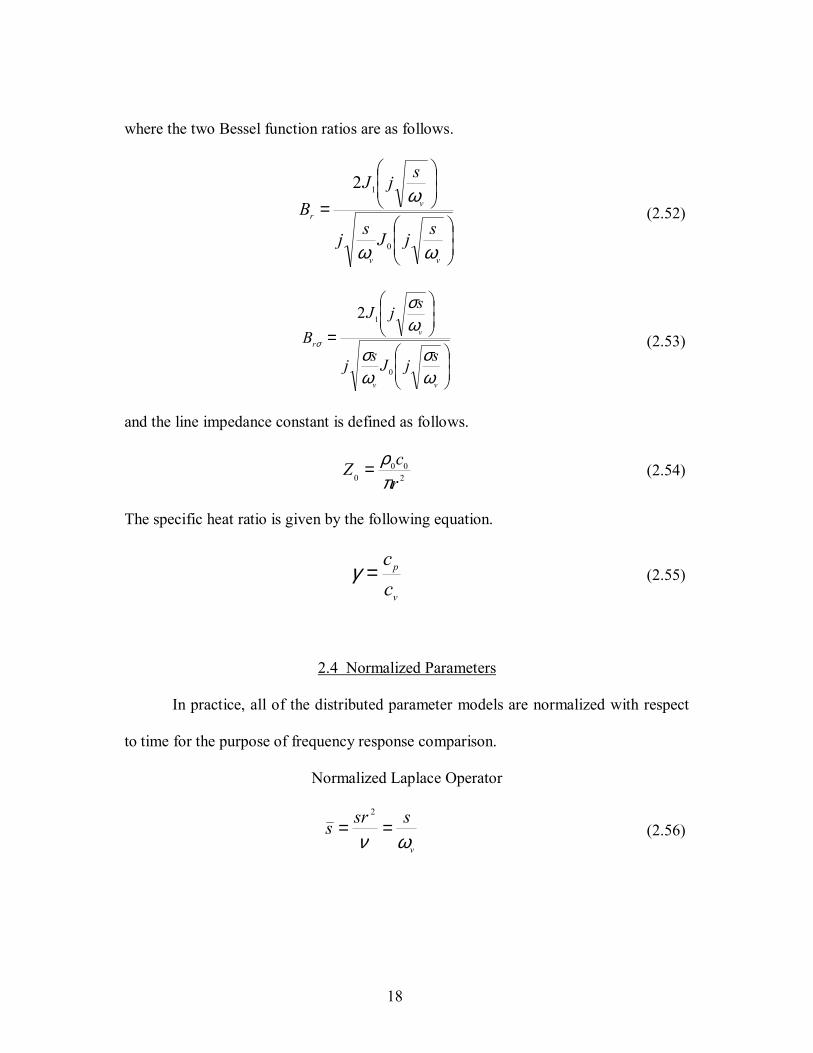
where the two Bessel function ratios are as follows.
=
vv
vr
sjJsj
sjJB
ωω
ω
0
12
(2.52)
=
vv
vr
sjJsj
sjJB
ωσ
ωσ
ωσ
σ
0
12 (2.53)
and the line impedance constant is defined as follows.
200
0 rcZ
πρ= (2.54)
The specific heat ratio is given by the following equation.
v
p
cc
=γ (2.55)
2.4 Normalized Parameters
In practice, all of the distributed parameter models are normalized with respect
to time for the purpose of frequency response comparison.
Normalized Laplace Operator
v
ssrsων
==2
(2.56)

19
Viscous Frequency
2rv
νω = (2.57)
Replacing the Laplace operator with the normalized operator produces the following.
vss ω= (2.58)
gives the normalized propagation operator as:
r
r
c
v
BBss
−−+=Γ
1)1(1)( σγ
ωω (2.59)
Defining the dissipation number as:
c
vnD
ωω= (2.60)
and simplifying the normalized propagation operator gives the following equation.
r
rn B
BsDs−−+=Γ
1)1(1)( σγ
(2.61)
The dissipation number is often a used as a reference point when comparing
various frequency responses. The dissipation number can also be written as:
20rcLDn
ν= (2.62)
The pressure waves in a fluid transmission line propagate at the speed of sound
in the line, c0, making the dissipative number a function of this value. The speed of
sound is a function of the fluid density and the compressibility (inverse of bulk
modulus) of the system.

20
The characteristic frequency is represented by the following relationship.
Lc
c0=ω (2.63)
The dissipative transmission line model approach is referred to as viscous theory
and has been proven to be the most accurate model.
100 101 102 103-20
-15
-10
-5
0
5
10
15
20
25
Normalized Frequency rad/sec
Dec
ibel
s
Dn=0.01
Dn=0.05
Dn=0.1
Dn=0.3
Dn=0.5
Figure 2.6 Frequency magnitude response of a blocked hydraulic line using the dissipative model

21
100 101 102 103-200
-150
-100
-50
0
50
100
150
200
Normalized Frequency rad/sec
Deg
rees Dn=0.01
Dn=0.5
Figure 2.7 Frequency phase response of a blocked hydraulic line using the dissipative
model
2.5 Transmission Line Model Comparison
This section applies each of the five models covered in the last section to a blocked fluid transmission line and compares the resulting frequency response plots.
Figure 2.8 Blocked transmission line illustration

22
Fluid Properties
Density = 870 Kg/m3
Kinematic Viscosity = 4.6e-5 m2/s
Prandtl Number = 1
Specific Heat Ratio = 1
Bulk Modulus = 1.21e9 N/m2
Line Properties
Length = 2 m
Diameter = 0.01 m
Bulk Modulus = 1.73e7 N/m2
2.5.1 Lumped Parameter Model
The lumped parameter approach requires the computation of values for the line
inertance and capacitance.
inoutin QLsRPP )( +=− (2.64)
outpin sPCQ = (2.65)
outsPCLsRPP poutin )( +=− (2.66)
outPRsCLsCP ppin )1( 2 ++= (2.67)
inPRsCLsC
Ppp
out )1(1
2 ++= (2.68)

23
4
128d
Rπ
νρl= (2.69)
54
s-N 3.261e8)01.0(
)2)(870)(56.4(128m
eR =−=π
(2.70)
AL lρ= (2.71)
5
2s-N2.215e7)2/01.0()2)(870(
2 mL ==
π (2.72)
ep
VCβ
= (2.73)
The effective bulk modulus of the system takes into account the compressibility
of both the hydraulic fluid and the hydraulic hose. The tangent bulk modulus is
measured at a specific point and pressure whereas the secant bulk modulus is average
change in pressure and volume. The secant bulk modulus is used in all computations.
ETVPVT
,0
∂∂−=β (2.74)
ETVPVs
,
∆∆−=β (2.75)
ETPV
Vs ,
11
∆∆−=
β (2.76)
ETETPV
VV
VPV
VV
V
hose
hosehose
fluid
fluidfluid
s ,,
1
∆
∆+
∆∆
−=β (2.77)

24
In this system the liquid is compressing and the hose is expanding which
explains the assignment of the positive and negative signs in the equation. The volume
of the system is also the volume of the hose and the equation can be rewritten as
follows.
ET
hose
ETfluid
fluidfluid
s PVV
PVV
VV
,,
1
∆∆+
∆∆
−=β (2.78)
EThoseETfluid
fluid
s VV
,,
111
+
=
βββ (2.79)
Assuming that the volume of the fluid is equal to the total volume gives
EThoseETfluids ,,
111
+
=
βββ (2.80)
hosefluid
hosefluidse ββ
ββββ
+== (2.81)
2 1.706e7
1.73e71.21e9
)(1.73e7)e9(1.21
m
Ne ==
+β (2.82)
( ) ( )Nm VC
ep
52
12-9.21ee771.1
22/01.0 === πβ
(2.83)
The transfer function for the lumped parameter model is:
inout PPses )133003.0(
1-3-0.20403e 2 ++
= (2.84)

25
2.5.2 Distributed Parameter Models
The distributed parameter matrix transfer function for this causality reduces to
Γ=
coshin
out
PP (2.85)
This transfer function will be applied to the next four models. The only
difference is in the calculation of the propagation operator. The impedance constant is
not required in this causality since the solution is the pressure output and not fluid flow.
2.5.2.1 Lossless Line Model
0
)(cLss =Γ (2.86)
ρβec =
0 (2.87)
m/s 140.2870
e771.10
==c (2.88)
ss .01428140.2
2s)( ==Γ (2.89)
2.5.2.2 Linear Friction Model
20
081)(
0src
Lssν
+=Γ (2.90)
ss
sess 72.1410143.0
)005.0()56.4(81
2.1402)( 2 +=−+=Γ (2.91)

26
2.5.2.3 Viscous Model
−
=Γ
νν
ν
srjJsrj
srjJ
c
sLs
2
0
2
2
12
1
)(
(2.92)
2.5.2.4 Dissipative Model
−
=Γ
vv
v
c
sjJsj
sjJ
ss
ωω
ωω
0
121
1)(
(2.93)
The viscous model and the dissipative model for the line have the same resulting
propagation operator as well as the same transfer function due to the fact that the
specific heat ratio of liquid is unity.

27
Figure 2.9 Frequency magnitude response of common fluid transmission line models

28
CHAPTER 3
MODAL APPROXIMATION APPROACH 3.1 Model Overview
As a result of being derived from partial differential equations the dissipative
model transfer function is not in the rational polynomial form familiar in system
modeling and control theory.
ΓΓΓ
ΓΓ−
Γ
=
out
in
c
c
in
out
Q
P
Z
Z
Q
P
cosh1
coshsinh
coshsinh
cosh1
(3.1)
Fluid line systems actually contain several components in addition to the fluid line or
lines.
Figure 3.1 Hydraulic log splitter

29
In order to integrate this model with other lumped parameters in a total system it
is necessary to approximate the resulting transfer function as a rational polynomial
transfer function. This effort has been the focus of much of the latest research in this
field.
There are four possible causalities to a fluid line problem as follows:
ΓΓ−
Γ
Γ−
ΓΓ
=
out
in
cc
cc
out
in
P
P
ZZ
ZZ
Q
Q
sinhcosh
sinh1
sinh1
sinhcosh
(3.2)
ΓΓ
−Γ
Γ−
ΓΓ
=
out
in
cc
cc
out
in
Q
Q
ZZ
ZZ
P
P
sinhcosh
sinh
sinhsinhcosh
(3.3)
ΓΓΓ−
ΓΓ
Γ
=
in
out
c
c
out
in
Q
P
Z
Z
Q
P
cosh1
coshsinh
sinhsinh
cosh1
(3.4)
ΓΓΓ
ΓΓ−
Γ
=
out
in
c
c
in
out
Q
P
Z
Z
Q
P
cosh1
coshsinh
coshsinh
cosh1
(3.5)
In these four equations are seven unique transfer functions that will be defined as
follows:
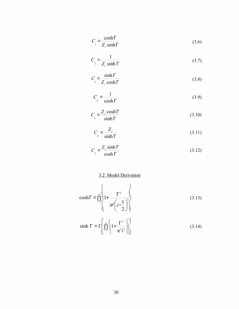
30
ΓΓ=
sinhcosh
1cZ
C (3.6)
Γ=
sinh1
2cZ
C (3.7)
ΓΓ=
coshsinh
3cZ
C (3.8)
Γ=
cosh1
4C (3.9)
ΓΓ=
sinhcosh
5
cZC (3.10)
Γ=
sinh6
cZC (3.11)
ΓΓ=
coshsinh
7
cZC (3.12)
3.2 Model Derivation
∏
−
Γ+=Γ∞
=12
2
2
21
1coshi
iπ
(3.13)
∏
+=Γ∞
=1i 22
2
iπΓ1Γsinh (3.14)

31
∏
=
∞
= +
+
12,0
2,1
1
1
i
i
ir s
s
Bασασ
σ (3.15)
∏
=
∞
= +
+
12,0
2,1
1
1
i
i
ir s
s
Bα
α (3.16)
Where:
σ is the Prandtl number
α0,i is the ith zero of the zero-order Bessel function
α1,i is the ith zero of the first-order Bessel function
The infinite product representation of the propagation operator is
∏
+
+−
∏
+
+−+
=Γ
∞
=
∞
=
1
2
,0
2
,1
1
2
,0
2
,1
1
11
1
1)1(1
)(
i
i
i
i
i
i
n
s
s
s
s
sDs
α
α
ασασ
γ
(3.17)

32
Multiply both the numerator and denominator terms by ∏
+
∞
=12,0
1i i
sα
and by
∏
+
∞
=12,0
1i i
sασ
appropriately and expanding to get the following equation:
( )
++
++−
+
+
++
++−+
+
+
=Γ
............
............
22,1
21,0
22,1
21,1
22,0
21,0
22,0
21,0
22,1
21,1
22,0
21,0
111111
1111111
)(
ασ
ασ
αααα
ααασ
ασγ
ασ
ασ
ssssss
ssssss
sDs n
(3.18)
This can be reduced to:
+++++++
=Γ mm
mm
n sbsbsbsasasa
sDs 22
221
22
221)(
L
Lγ (3.19)
The polynomial coefficients ai and bi are functions of the Prandtl number and m only.
3.2.1 Modal Approximation of 1/cosh Γ
This result is applied to the series equation for cosh Γ.
∏
=∞
=
+++
++++
−
+Γ
1 22
221
22
221
22
22
21
1coshi m
m
mmn
sbsbsbsasasa
i
sDL
Lγ
π (3.20)
A new variable called the dimensionless root index for cosh Γ is introduced:
−=
211 i
Dncλ i = 1,2,3��� (3.21)

33
∏=∞
=
+++
+++++Γ1 2
22
21
22
221
22
21cosh
i mm
mm
c sbsbsbsasasas
L
Lγλπ (3.22)
The goal is to simplify the equation as a rational polynomial first by combining the
unity term and series term as follows.
( ) ( )
( )∏
=∞
=−
−
+++
++++++++Γ
112
2
2
21
2
2
2
2122
212
2
2
21
coshi
m
m
m
m
c
m
m
sbsbsb
sasasassbsbsb
L
LL γλπ
(3.23)
Then divide both the numerator and denominator by s to get:
( ) ( )( )∏
=∞
=−
−
+++
++++++++Γ
112
221
22
22122
12221
coshi
mm
mm
c
mm
sbsbb
sasasassbsbb
L
LL γλπ
(3.24)
Combining terms in the numerator results in:
( )( )∏= ∞
=−
++
+++++++Γ
112
22
21
1222
2321cosh
im
m
mm
sbsbsbscscscb
L
L (3.25)
The polynomial coefficients bi are functions of the Prandtl number and m only
whereas the polynomial coefficients ci are functions of the Prandtl number, m, the
specific heat ratio, and the dimensionless root index.
Factoring the numerator and denominator results in the following equation:

34
( )( ) ( )( )( ) ( )∏=
∞
=
+++
++++Γ−1 1221
22
21
..........cosh 2
i m
vivii
pspspssszszs ωως
(3.26)
The real root terms in both the numerator and the denominator virtually cancel each
other out for lines with low damping and cosh Γ can be approximated as:
∏=∞
=
+++Γ
1
22 2coshi cici
ninii
bsass ωως
(3.27)
The transfer function 1/cosh Γ is:
∑== ++
+Γ
n
i
inini
cici
ssbsa
122 2cosh
1ωως (3.28)
n = number of second order modes
The values for the coefficients have been tabulated.
3.2.2 Modal Approximation of Ζc sinh Γ/cosh Γ
Substitute the infinite product series form for sinh Γ and cosh Γ.
∏
−
Γ+
∏
Γ+Γ
=ΓΓ
∞
=
∞
=
12
2
2
1 22
2
21
1
1
coshsinh
i
i
cc
i
iZZ
π
π
(3.29)
Substitute in the equation for the propagation operator.

35
∏
−−+
−
+
∏
−−++
−−+=
ΓΓ
∞
=
∞
=
12
2
22
1 22
22
1)1(1
21
1
1)1(11
1)1(1
coshsinh
i r
rn
ir
rn
r
rnc
c
BB
i
sD
BB
isD
BBsDZZ
σ
σ
σ
γ
π
γπγ
(3.30)
Substitute the equation for the characteristic impedance.
∏
−−+
−
+
∏
−−+
+
−−+
−+−=
ΓΓ
∞
=
∞
=
1 2
2
22
1 22
22
0
1)1(1
21
1
1)1(1
1
1)1(1
))1(1)(1(coshsinh
ir
rn
ir
rn
r
rn
rr
c
BB
i
sD
BB
isD
BB
sDBB
ZZ
σ
σ
σ
σ
γ
π
γπγ
γ
(3.31)
The matrix transfer function when modal approximation method is applied is in
the following form to remove the Z0 term in the development of the modal
approximation model of the individual terms.
ΓΓΓ
ΓΓ
−Γ
=
out
in
c
c
in
out
QZ
P
Z
ZZ
QZ
P
0
0
0 cosh1
coshsinh
coshsinh
cosh1
(3.32)
∏
−−+
−
+
∏
−−++
−−+
−+−=
ΓΓ
∞
=
∞
=
12
2
22
1 22
22
0
1)1(1
21
1
1)1(11
1)1(1
))1(1)(1(1
coshsinh
ir
rn
ir
rn
r
rn
rr
c
BB
i
sD
BB
isD
BB
sDBBZ
Z
σ
σ
σ
σ
γ
π
γπγ
γ
(3.33)
Reducing Bessel function terms gives

36
∏
−−+
−
+
∏
−−++
−=
ΓΓ
∞
=
∞
=
12
2
22
1 22
22
0
1)1(1
21
1
1)1(11
)1(coshsinh
ir
rn
ir
rn
r
nc
BB
i
sD
BB
isD
BsD
ZZ
σ
σ
γ
π
γπ
(3.34)
Substitute the infinite product series form of the Bessel functions produces:
∏
∏
+
+
−
∏
+
+
−+
−
+
∏
∏
+
+
−
∏
+
+
−+
+
∏
+
+
−
=ΓΓ
∞
=
∞
=
∞
=
∞
=
∞
=
∞
=
∞
=
1
1
2,0
2,1
1
2,0
2,1
2
2
22
1
1
2,0
2,1
1
2,0
2,1
22
22
1
2,0
2,1
0
1
1
1
1
1
)1(1
21
1
1
1
1
1
1
)1(1
1
1
1
1
coshsinh
i
i
i
i
i
i
i
n
i
i
i
i
i
i
i
n
i
i
i
nc
s
s
s
s
i
sD
s
s
s
s
isD
s
ssD
ZZ
α
α
ασασ
γ
π
α
α
ασασ
γ
π
α
α
(3.35)
Multiply both the numerator and denominator terms by ∏
+
∞
=1 2,0
1i i
sα
and by
∏
+
∞
=1 2,0
1i i
sασ
appropriately to get the following equation:

37
∏
∏
+−∏
+∏ +
∏
+−+∏
+∏ +
−
+
∏
∏
+−∏
+∏ +
∏
+−+∏
+∏ +
+
∏ +−∏ +
∏ +
=Γ
Γ
∞
=
∞
=
∞
=
∞
=
∞
=
∞
=
∞
=
∞
=
∞
=
∞
=
∞
=
∞
=
∞
=
∞
=
∞
=
∞
=
∞
=
1
1 2
,1
1 2
,0
1 2
,0
1 2
,1
1 2
,0
1 2
,0
2
2
22
1
1 2
,1
1 2
,0
1 2
,0
1 2
,1
1 2
,0
1 2
,0
22
22
1 2
,11 2
,0
1 2
,0
0
111
1)1(11
2
11
111
1)1(11
1
11
1
cosh
sinh
i
i
i
i
i
ii
i
i
i
i
ii
n
i
i
i
i
i
ii
i
i
i
i
ii
n
ii
ii
ii
n
c
sss
sss
i
sD
sss
sss
i
sD
ss
s
sDZ
Z
ααα
σ
α
σγ
α
σ
α
π
ααα
σ
α
σγ
α
σ
α
π
αα
α (3.36)
Another dimensionless root index for the sinh Γ polynomial is introduced.
ns D
i=λ (3.37)
Substitute the dimensionless root indices of both cosh Γ and sinh Γ into the equation.
∏
∏
+−∏
+∏ +
∏
+−+∏
+∏ +
+
∏
∏
+−∏
+∏ +
∏
+−+∏
+∏ +
+
∏ +−∏ +
∏ +
=Γ
Γ
∞
=∞
=
∞
=
∞
=
∞
=
∞
=
∞
=
∞
=∞
=
∞
=
∞
=
∞
=
∞
=
∞
=
∞
=
∞
=
∞
=
1
1 2,1
1 2,0
1 2
,0
1 2,1
1 2,0
1 2
,0
22
2
1
1 2,1
1 2,0
12
,0
1 2,1
1 2,0
12
,0
22
2
1 2
,11 2
,0
12
,0
0
111
1)1(11
1
111
1)1(11
1
11
1
cosh
sinh
i
ii
ii
ii
ii
ii
ii
c
i
ii
ii
ii
ii
ii
ii
s
ii
ii
ii
nc
sss
sss
s
sss
sss
s
ss
s
sDZ
Z
ααα
σ
α
σγα
σ
α
λπ
ααα
σ
α
σγ
α
σ
α
λπ
αα
α
(3.38)

38
This equation can be simplified into the following form.
[ ] [ ][ ]∏ +++++
∏ +++++
++++++
=ΓΓ
∞
=−
∞
=−
1
221221
1
221221
21
21
0 )2)().....()((
)2)().....()((
)).....()(()).....()((
coshsinh
iviviim
ivsivsisim
m
mc
sspspsps
ssrsrsrs
lslslsususus
ZZ
ωωζ
ωωζ
(3.39)
The real root terms in both the numerator and the denominator do not
necessarily cancel each other out for lines with low damping as in the case of cosh Γ.
If ΓΓ
coshsinh
0ZZc is divided by the first real root )( 1us + , the residues of the resulting real
roots approach zero.
∑++
++=
ΓΓ
=
n
i vivii
zizic
ss
bsaus
ZZ
12210 2
)(coshsinh
ωωζ (3.40)
n = number of second order modes
The values for the coefficients have been tabulated.
3.2.3 Modal Approximation of sinh Γ / Ζc cosh Γ
As stated earlier, the form of the transfer function when the Modal
Approximation method is applied is in the following form to remove the Z0 term in the
development of the modal approximation model of the individual terms.
ΓΓ
coshsinh0
cZZ (3.41)
Substitute the infinite product series form for sinh Γ and cosh Γ.

39
∏
−
Γ+
∏
+
=ΓΓ
∞
=
∞
=
12
2
2
1i 22
2
00
21
1
iπΓ1Γ
coshsinh
ic
c
iZ
Z
ZZ
π
(3.42)
Substitute in the equation for the propagation operator.
∏
−
−−+
+
∏
−−+
+−−+
=ΓΓ
∞
=
∞
=
12
2
22
1i 22
22
0
0
21
1)1(1
1
iπ1
)1(1
11
)1(1
coshsinh
i
r
rn
c
r
rn
r
rn
c
i
BBsD
Z
BBsD
BBsDZ
ZZ
π
γ
γγ
σ
σ
σ
(3.43)
Substitute in the equation for the characteristic impedance.
∏
−
−−+
+−+−
∏
−−+
+−−+
=ΓΓ
∞
=
∞
=
12
2
22
0
1i 22
22
0
0
21
1)1(1
1))1(1)(1(
iπ1
)1(1
11
)1(1
coshsinh
i
r
rn
rr
r
rn
r
rn
c
i
BBsD
BBZ
BBsD
BBsDZ
ZZ
π
γ
γ
γγ
σ
σ
σ
σ
(3.44)
Reducing Bessel function terms and canceling out the impedance constant gives

40
[ ]
∏
−
−−+
+
∏
−−+
+
−+=ΓΓ
∞
=
∞
=
12
2
22
1i 22
22
0
21
1)1(1
1
iπ1
)1(1
1
))1(1(coshsinh
i
r
rn
r
rn
rnc
i
BBsD
BBsD
BsDZZ
π
γ
γ
γσ
σ
σ
(3.45)
Substitute the infinite product series form of the Bessel functions produces
∏
∏
+
+−
∏
+
+−+
−
+
∏
∏
+
+−
∏
+
+−+
+
∏
+
+−+=
ΓΓ
∞
=
∞
=
∞
=
∞
=
∞
=
∞
=
∞
=
1
1
2,0
2,1
1
2,0
2,1
2
2
22
1i
1
2,0
2,1
1
2,0
2,1
22
22
1
2,0
2,10
1
11
1
1)1(1
21
1
1
11
1
1)1(1
iπ1
1
1)1(1
coshsinh
i
i
i
i
i
i
i
n
i
i
i
i
i
i
n
i
i
in
c
s
s
s
s
i
sD
s
s
s
s
sD
s
s
ZZ
sD
α
α
ασασ
γ
π
α
α
ασασ
γ
ασασ
γ
(3.46)
Combine the following term as one quotient.

41
∏
+
+−+
∞
=1
2
,0
2
,1
1
1)1(1
i
i
i
s
s
ασασ
γ (3.47)
To get the following:
∏
+
∏
+−+∏
+
∞
=
∞
=
∞
=
1 2,0
1 2,1
1 2,0
1
1)1(1
ii
ii
ii
s
ss
ασ
ασγ
ασ
(3.48)
Substitute into the equation to get
∏
∏
+
+−
∏
+
∏
+−+∏
+
−
+
∏
∏
+
+−
∏
+
∏
+−+∏
+
+
∏
+
∏
+−+∏
+=
ΓΓ
∞
=
∞
=
∞
=
∞
=
∞
=
∞
=
∞
=
∞
=
∞
=
∞
=
∞
=
∞
=
∞
=
1
1
2,0
2,1
1 2,0
1 2,1
1 2,0
2
2
22
1i
1
2,0
2,1
1 2,0
1 2,1
1 2,0
22
22
1 2,0
1 2,1
1 2,00
1
11
1
1)1(1
21
1
1
11
1
1)1(1
iπ1
1
1)1(1
coshsinh
i
i
i
i
ii
ii
ii
n
i
i
i
ii
ii
ii
n
ii
ii
ii
nc
s
s
s
ss
i
sD
s
s
s
ss
sD
s
ss
ZZ
sD
α
α
ασ
ασγ
ασ
π
α
α
ασ
ασγ
ασ
ασ
ασγ
ασ
(3.49)
Combine the following term as one quotient

42
∏
+
+−
∞
=1
2,0
2,1
1
11
i
i
i
s
s
α
α (3.50)
To get the following
∏
+
∏
++∏
+
∞
=
∞
=
∞
=
1 2,0
1 2,1
1 2,0
1
11
ii
ii
ii
s
ss
α
αα (3.51)
Substitute into the equation to get
∏
∏
+
∏
++∏
+
∏
+
∏
+−+∏
+
−
+
∏
∏
+
∏
++∏
+
∏
+
∏
+−+∏
+
+
∏
+
∏
+−+∏
+=
ΓΓ
∞
=
∞
=
∞
=
∞
=
∞
=
∞
=
∞
=
∞
=
∞
=
∞
=
∞
=
∞
=
∞
=
∞
=
∞
=
∞
=
∞
=
1
1 2
,0
1 2
,1
1 2
,0
1 2
,0
1 2
,1
1 2
,0
2
2
22
1i
1 2
,0
1 2
,1
1 2
,0
1 2
,0
1 2
,1
1 2
,0
22
22
1 2
,0
1 2
,1
1 2
,00
1
11
1
1)1(1
21
1
1
11
1
1)1(1
iπ1
1
1)1(1
coshsinh
i
i
i
i
i
i
i
i
i
i
i
i
i
n
i
i
i
i
i
i
i
i
i
i
i
i
n
i
i
i
i
i
i
n
c
s
ss
s
ss
i
sD
s
ss
s
ss
sD
s
ss
ZZ
sD
α
αα
ασ
ασγ
ασ
π
α
αα
ασ
ασγ
ασ
ασ
ασγ
ασ
(3.52)
Factor out the following term.

43
∏
+
∏
+
∞
=
∞
=
1 2,0
1 2,0
1
1
ii
ii
s
s
ασα (3.53)
The result is the following equation.
∏
∏
++∏
+
∏
+−+∏
+
∏
+
∏
+
−
+
∏
∏
++∏
+
∏
+−+∏
+
∏
+
∏
+
+
∏
+
∏
+−+∏
+=
ΓΓ
∞
=∞
=
∞
=
∞
=
∞
=
∞
=∞
=
∞
=
∞
=
∞
=
∞
=
∞
=
∞
=
∞
=
∞
=
∞
=
∞
=
1
1 2
,1
1 2
,0
1 2
,1
1 2
,0
2
2
22
1i
1 2
,1
1 2
,0
1 2
,1
1 2
,0
22
22
1 2
,0
1 2
,1
1 2
,00
11
1)1(1
1
1
21
1
11
1)1(1
1
1
iπ1
1
1)1(1
coshsinh
1 2,0
1 2,0
1 2,0
1 2,0
i
i
i
i
i
i
i
i
in
i
i
i
i
i
i
i
in
i
i
i
i
i
i
n
c
ss
ss
s
s
i
sD
ss
ss
s
s
sD
s
ss
ZZ
i i
i i
i i
i i
sD
αα
ασγ
ασ
ασ
α
π
αα
ασγ
ασ
ασ
α
ασ
ασγ
ασ
(3.54)
Introduce the dimensionless root indices to get the following equation.
∏
∏
++∏
+
∏
+−+∏
+
∏
+
∏
+
+
∏
∏
++∏
+
∏
+−+∏
+
∏
+
∏
+
+
∏
+
∏
+−+∏
+
=ΓΓ
∞
= ∞
=
∞
=
∞
=
∞
=
∞
= ∞
=
∞
=
∞
=
∞
=
∞
=
∞
=
∞
=
∞
=
∞
=
∞
=
∞
=
1
1 2,11 2
,0
1 2,11 2
,0
2,0
2,0
22
2
1i
1 2,11 2
,0
1 2,11 2
,0
2,0
2,0
22
2
1 2,0
1 2,11 2
,00
11
1)1(1
1
1
1
11
1)1(1
1
1
π1
1
1)1(1
coshsinh
1
1
1
1
i
i ii i
i ii i
i
i
c
i ii i
i ii i
i
i
s
i i
i ii in
c
ss
ss
s
s
s
ss
ss
s
s
s
s
ss
ZZ
i
i
i
i
sD
αα
ασγ
ασ
ασ
α
λπ
αα
ασγ
ασ
ασ
αλ
ασ
ασγ
ασ
(3.55)
This equation can be simplified into the following form.
[ ][ ]∏ +++++
∏ +++++
+++
+++=
ΓΓ
∞
= −
∞
= −
1
221221
1
221221
21
21
0 )2)().....()((
)2)().....()((
)).....()((
)).....()((
coshsinh
i viviim
i vsivsisim
m
mn
c
sspspsps
ssrsrsrs
bsbsbs
asasassD
ZZ
ωωζ
ωωζ
(3.56)

44
The real root terms in both the numerator and the denominator do not
necessarily cancel each other out for lines with low damping as in the case of cosh Γ.
If ΓΓ
coshsinh
0ZZc is divided by the Laplace operator, the residues of the resulting real roots
approach zero.
( ) ( )∑=
+
++
++
+++
=Γ
Γ n
ivivii
sisic
psk
psk
ssbsa
ZsZ
12
2
1
122
0
...2cosh
sinhωωζ
(3.57)
The inclusion of one real pole gives a very accurate approximation.
∑=
+++
++
=Γ
Γ n
ivivii
sisic
ssbsa
psk
ZsZ
1 220
0
02(cosh
sinh) ωωζ
(3.58)
3.3 Modal Approximation Residue Coefficient Tables
Table 3.1 Residue Coefficients for Air (Pneumatic Transmission Lines) Zc/sinh Γ 1/Zc sinh Γ 1/cosh Γ
(-1)iDnai/Z0 (-1)iDnbbi/Z0 (-1)iZ0Dnai (-1)iZ0Dnbi
Zc cosh Γ/sinh Γ Zc sinh Γ/cosh Γ
cosh Γ/Zc sinh Γ sinh Γ/Zc cosh Γ
λc
lc λs
ωn ζ (-1)i+1(1-2i)ai (-1)i+1(1-2i)bi
Dnai/Z0 Dnbi/Z0 Z0Dnai Z0Dnbi 0.02 0.0451 64.163 -0.000159 -0.002586 1.4286 8.2617 1.3797 -2.14E-50.04 0.0901 32.083 -0.000635 -0.010345 1.4287 8.2618 1.3798 -8.54E-50.06 0.1352 21.390 -0.001428 -0.023279 1.4288 8.2618 1.3800 -1.92E-40.08 0.1803 16.045 -0.002539 -0.041390 1.4289 8.2619 1.3802 -3.40E-40.10 0.2254 12.838 -0.003966 -0.064685 1.4291 8.2621 1.3805 -5.31E-40.20 0.4509 6.4266 -0.015830 -0.25915 1.4306 8.2631 1.3829 -0.002080.30 0.6768 4.2930 -0.035494 -0.58462 1.4332 8.2650 1.3869 -0.004510.40 0.9032 3.2288 -0.062787 -1.0431 1.4369 8.2677 1.3925 -0.007590.50 1.1304 2.5922 -0.097464 -1.6375 1.4416 8.2714 1.3996 -0.011010.60 1.3584 2.1695 -0.13919 -2.3713 1.4473 8.2762 1.4083 -0.014360.70 1.5875 1.8688 -0.18755 -3.2489 1.4542 8.2822 1.4185 -0.017130.80 1.8177 1.6444 -0.24200 -4.2751 1.4620 8.2898 1.4301 -0.018730.90 2.0493 1.4708 -0.30192 -5.4556 1.4710 8.2991 1.4431 -0.018481.00 2.2824 1.3327 -0.36653 -6.7962 1.4809 8.3105 1.4573 -0.015631.20 2.7535 1.1272 -0.50624 -9.9828 1.5038 8.3406 1.4887 0.001035

45
Table 3.1 � Continued 1.30 2.9917 1.0488 -0.57924 -11.841 1.5166 8.3600 1.5055 0.016461.35 3.1115 1.0142 -0.61602 -12.839 1.5233 8.3709 1.5140 0.026261.38 3.1836 0.99459 -0.6381 -13.460 1.5274 8.3779 1.5192 0.032861.40 3.2317 0.98202 -0.6528 -13.884 1.5302 8.3827 1.5227 0.037571.50 3.4737 0.92437 -0.7257 -16.116 1.5444 8.4091 1.5400 0.064962.00 4.7114 0.72401 -1.0434 -30.217 1.6199 8.5995 1.6170 0.300863.00 7.2868 0.52103 -1.3385 -72.731 1.7364 9.1569 1.6597 0.953334.00 9.9163 0.41536 -1.5376 -133.45 1.7917 9.6372 1.6268 1.24165.00 12.571 0.35102 -1.8441 -213.52 1.8236 10.007 1.6052 1.2040
10.00 26.286 0.22229 -3.4749 -940.55 1.9113 12.073 1.6641 0.5700215.00 40.539 0.17476 -4.2906 -2230.3 1.9395 14.396 1.7273 0.8377020.00 55.034 0.14745 -4.8375 -4084.1 1.9494 16.347 1.7617 1.272525.00 69.661 0.12923 -5.2970 -6508.5 1.9547 18.016 1.7838 1.670430.00 84.376 0.11602 -5.6900 -9508.2 1.9581 19.506 1.7997 2.047235.00 99.157 0.10588 -6.0263 -13086 1.9605 20.868 1.8119 2.418240.00 113.99 0.09778 -6.3149 -17243 1.9622 22.131 1.8215 2.787945.00 128.86 0.09112 -6.5633 -21982 1.9635 23.331 1.8294 3.157650.00 143.76 0.08551 -6.7775 -27302 1.9644 24.427 1.8358 3.527155.00 158.69 0.08071 -6.9623 -33204 1.9652 25.482 1.8413 3.896460.00 173.64 0.07653 -7.1213 -39690 1.9657 26.486 1.8459 4.265470.00 203.59 0.06958 -7.3734 -54410 1.9665 28.364 1.8534 5.002480.00 233.60 0.06400 -7.5525 -71464 1.9669 30.095 1.8591 5.737290.00 263.66 0.05937 -7.6720 -90851 1.9671 31.703 1.8536 6.4684
100.00 293.74 0.05547 -7.7425 -112572 1.9672 33.205 1.8774 7.1946150.00 444.46 0.04220 -7.6011 -256130 1.9663 39.516 1.8814 10.698200.00 595.39 0.03429 -7.0233 -457800 1.9647 44.366 1.8714 13.883300.00 897.35 0.02500 -5.5689 -1034823 1.9617 51.192 1.8836 19.052400.00 1199.2 0.01964 -4.2872 -1842813 1.9595 55.539 1.8835 22.734500.00 1500.8 0.01614 -3.3103 -2881478 1.9579 58.387 1.8830 25.300600.00 1802.3 0.01367 -2.5920 -4150748 1.9568 60.313 1.8825 27.099700.00 2103.8 0.01185 -2.0646 -5650623 1.9560 61.655 1.8820 28.384800.00 2405.1 0.01044 -1.6728 -7381119 1.9554 62.619 1.8816 29.321900.00 2706.4 0.00933 -1.3771 -9342256 1.9550 63.330 1.8814 30.019
1000.00 3007.5 0.00843 -1.1501 -11534000 1.9547 63.866 1.8811 30.550

46
Table 3.2 Residue Coefficients for Liquid (Hydraulic Transmission Lines) Zc/sinh Γ 1/Zc sinh Γ
1/cosh Γ (-1)iDnai/Z0 (-1)iDnbbi/Z0 (-1)iZ0Dnai (-1)iZ0Dnbi
Zc cosh Γ/sinh Γ Zc sinh Γ/cosh Γ
cosh Γ/Zc sinh Γ sinh Γ/Zc cosh Γ
λc
lc λs
ωn ζ (-1)i+1(1-2i)ai (-1)i+1(1-2i)bi
Dnai/Z0 Dnbi/Z0 Z0Dnai Z0Dnbi 0.01 0.0267 108.31 -6.7412E-6 -9.0755E-4 2.0000 11.566 1.3824 -7.6476E-60.02 0.0534 54.154 -2.6965E-5 -3.6302E-3 2.0000 11.566 1.3824 -3.0590E-50.03 0.0801 36.103 -6.0670E-5 -8.1680E-3 2.0000 11.566 1.3824 -6.8828E-50.04 0.1068 27.077 -1.0786E-4 -1.4521E-2 2.0000 11.566 1.3824 -1.2236E-40.05 0.1335 21.662 -1.6852E-4 -2.2689E-2 2.0000 11.566 1.3824 -1.9118E-40.06 0.1602 18.052 -2.4267E-4 -3.2672E-2 2.0000 11.566 1.3824 -2.7530E-40.07 0.1869 15.473 -3.3030E-4 -4.4471E-2 2.0000 11.566 1.3824 -3.7471E-40.08 0.2136 13.339 -4.3141E-4 -5.8084E-2 2.0000 11.566 1.3824 -4.8941E-40.09 0.2403 12.035 -5.4599E-4 -7.3513E-2 2.0000 11.567 1.3824 -6.1940E-40.10 0.2670 10.832 -6.7404E-4 -9.0758E-2 2.0000 11.567 1.3824 -7.6467E-40.20 0.5340 5.4172 -2.6952E-3 -3.6306E-1 2.0001 11.567 1.3825 -3.0577E-30.30 0.8010 3.6130 -6.0607E-3 -8.702E-1 2.0003 11.568 1.3828 -6.8764E-30.40 1.0681 2.7113 -1.0765E-2 -1.4528 2.0005 11.569 1.3831 -1.2216E-20.50 1.3352 2.1707 -1.6803E-2 -2.2706 2.0007 11.571 1.3835 -1.9069E-20.60 1.6023 1.8106 -2.4165E-2 -3.2707 2.0011 11.573 1.3840 -2.7428E-20.70 1.8696 1.5536 -3.2840E-2 -4.4535 2.0015 11.575 1.3846 -3.7283E-20.80 2.1369 1.3611 -4.2817E-2 -5.8194 2.0019 11.578 1.3852 -4.8619E-20.90 2.4043 1.2116 -5.4081E-2 -7.3689 2.0024 11.581 1.3860 -6.1425E-21.00 2.6718 1.0921 -6.6615E-2 -9.1026 2.0030 11.584 1.3868 -7.5681E-21.05 2.8056 1.0410 -7.3354E-2 -10.039 2.0033 11.586 1.3873 -8.3351E-21.10 2.9394 0.9945 -8.0403E-2 -11.021 2.0036 11.588 1.3878 -9.1376E-21.20 3.2072 0.9134 -9.5425E-2 -13.125 2.0043 11.593 1.3888 -1.0849E-11.30 3.4751 0.8448 -1.1166E-1 -15.414 2.0050 11.597 1.3899 -1.2698E-11.40 3.7432 0.7862 -1.2908E-1 -17.891 2.0058 11.603 1.3911 -1.4686E-11.60 4.2796 0.6912 -1.6739E-1 -23.408 2.0075 11.615 1.3937 -1.9062E-11.80 4.8171 0.6177 -2.1015E-1 -29.684 2.0094 11.629 1.3967 -2.3954E-12.00 5.3553 0.5593 -2.5710E-1 -36.725 2.0114 11.645 1.4000 -2.9338E-13.00 8.0609 0.3868 -5.4497E-1 -83.734 2.0242 11.765 1.4206 -6.2620E-14.00 10.796 0.3036 -8.9161E-1 -151.34 2.0394 11.967 1.4472 -1.03385.00 13.566 0.2554 -1.2545 -240.78 2.0550 12.267 1.4775 -1.469910.0 27.867 0.1613 -2.4968 -1037.6 2.0957 14.935 1.6156 -3.090315.0 42.640 0.1262 -3.0243 -2419.6 2.0904 17.737 1.6885 -3.899520.0 57.558 0.1061 -3.4562 -4388.6 2.0808 19.996 1.7294 -4.555925.0 72.570 0.0930 -3.8498 -6952.0 2.0736 21.941 1.7571 -5.162830.0 87.647 0.0836 -4.2000 -10113 2.0680 23.698 1.7776 -5.705635.0 102.77 0.0764 -4.5144 -13875 2.0634 25.313 1.7934 -6.195240.0 117.94 0.0707 -4.8011 -18238 2.0596 26.815 1.8062 -6.642845.0 133.14 0.0661 -5.0651 -23204 2.0564 28.223 1.8167 -7.056250.0 148.36 0.0622 -5.3101 -28774 2.0536 29.552 1.8256 -7.440455.0 163.60 0.0589 -5.5387 -34950 2.0511 30.813 1.8332 -7.799560.0 178.86 0.0560 -5.7528 -41731 2.0490 32.017 1.8398 -8.1363

47
Table 3.2 - Continued 70.0 209.43 0.0513 -6.1438 -57113 2.0454 34.275 1.8508 -8.752880.0 240.05 0.0475 -6.4932 -74925 2.0424 36.369 1.8596 -9.304990.0 270.71 0.0444 -6.8079 -95171 2.0399 38.327 1.8668 -9.8032100 301.41 0.0418 -7.0929 -1.1785E5 2.0377 40.172 1.8728 -1.0255E1150 455.23 0.0330 -8.1857 -2.6786E5 2.0303 48.150 1.8930 -1.1999E1200 609.32 0.0278 -8.8940 -4.7895E5 2.0257 54.724 1.9045 -1.3143E1250 763.82 0.0243 -9.3460 -7.5117E5 2.0224 60.376 1.9120 -1.3885E1300 918.36 0.0217 -9.6132 -1.0846E6 2.0200 65.354 1.9172 -1.4337E1350 1073.0 0.0197 -9.7418 -1.4791E6 2.0180 69.807 1.9211 -1.4572E1400 1227.7 0.0180 -9.7642 -1.9348E6 2.0164 73.831 1.9241 -1.4639E1450 1382.4 0.0166 -9.7046 -2.4515E6 2.0150 77.496 1.9264 -1.4576E1500 1537.2 0.0155 -9.5817 -3.0294E6 2.0138 80.850 1.9283 -1.4414E1550 1692.0 0.0145 -9.4101 -3.6683E6 2.0128 83.933 1.9298 -1.4174E1600 1846.8 0.0136 -9.2018 -4.3683E6 2.0119 86.776 1.9310 -1.3875E1650 2001.6 0.0129 -8.9662 -5.1293E6 2.0111 89.402 1.9320 -1.3532E1700 2156.4 0.0122 -8.7111 -5.9513E6 2.0103 91.834 1.9329 -1.3157E1800 2466.1 0.0110 -8.1668 -7.7783E6 2.0090 96.182 1.9342 -1.2351E1900 2775.7 0.0100 -7.6061 -9.8490E6 2.0080 99.937 1.9351 -1.1515E1
1000 3085.4 0.0092 -70529 -1.2164E7 2.0071 103.19 1.9358 -1.0686E1
Table 3.3 Residue Coefficients for the Real Poles of Z0 / sinh Γ and Z0 cosh Γ / sinh Γ
j Pole Residue Coefficients for Z0 / sinh Γ and
Z0 cosh Γ / sinh Γ Kj Dn / Z0
1 -10.1400 0.169386 2 -45.1979 0.046074 3 -107.923 0.019571 4 -198.487 0.010568 5 -316.905 0.006128 6 -462.886 0.004161 7 -638.069 0.003323 8 -837.815 0.000873 9 -1069.95 0.001907 10 -1326.08 0.000560

48
Table 3.4 Residue Coefficients for the Real Poles of 1/Z0 sinh Γ and cosh Γ/Z0 sinh Γ
j Pole Residue Coefficients for 1 / Z0 sinh Γ and
cosh Γ / Z0 sinh Γ Kj Dn / Z0
0 -5.78319 0.689837 1 -30.4713 0.129436 2 -74.8862 0.51558 3 -139.043 0.26872 4 -222.939 0.016075 5 -326.461 0.009828 6 -450.314 0.007266 7 -592.386 0.004908 8 -756.437 0.003949 9 -938.303 0.001649
3.4 Modal Approximation of a Blocked Hydraulic Line
The tabulated values for residue coefficients are a function of the dimensionless
root Indices cλ and sλ which are functions of the dissipative number, nD .
0.0262822 )0.01/2(140.0)(
5)(2)-(4.6e ===cr
LDn
ν (3.59)
For a four mode approximation (i=1,2,3,4):
−=
21
02628.01 i
Cλ (3.60)
][ 133.17 95.12 57.07 19.02 =C
λ (3.61)

49
10-2
10-1
100
101
102
10310
-2
10-1
100
101
102
103
104
Dimensionless Root Index, λc or λs
Nat
ural
Fre
quen
cy, ω
n
Figure 3.2 Log-log plot of natural frequency of a hydraulic line as a function of the dimensionless root index
Interpolation gives the following values for the natural frequencies for each mode.
403.45] 286.43 169.92 54.65[=C
ω (3.62)

50
10-2
10-1
100
101
102
103
10-3
10-2
10-1
100
101
102
103
Dam
ping
Rat
io, ζ n
Dimensionless Root Index, λc or λs
Figure 3.3 Log-log plot of natural frequency of a hydraulic line as a function of the dimensionless root index
Interpolation gives the following values for the damping ratios for each mode.
0.0360] 0.0431 0.0577 1100.0[=ς (3.63)
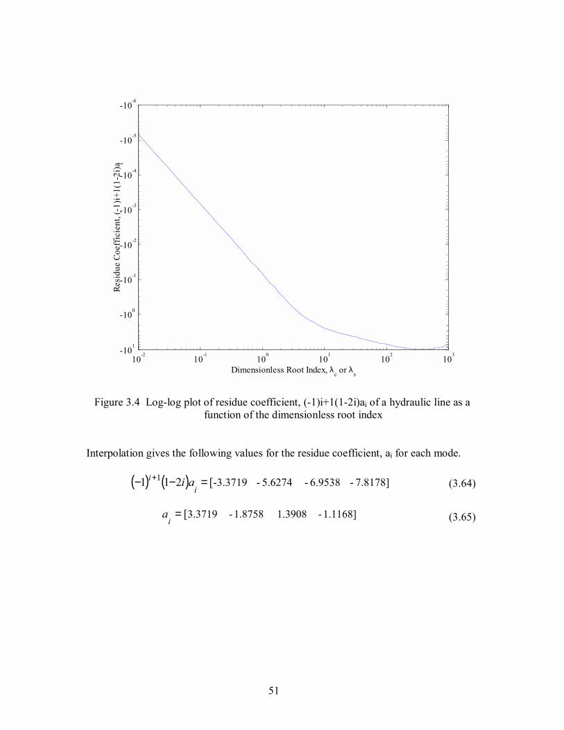
51
10-2
10-1
100
101
102
103-10
1
-100
-10-1
-10-2
-10-3
-10-4
-10-5
-10-6
Resi
due
Coef
ficie
nt, (
-1)i+
1(1-
2i)a i
Dimensionless Root Index, λc or λs
Figure 3.4 Log-log plot of residue coefficient, (-1)i+1(1-2i)ai of a hydraulic line as a function of the dimensionless root index
Interpolation gives the following values for the residue coefficient, ai for each mode.
( ) ( ) 7.8178]- 6.9538- 5.6274- -3.3719[211 1 =−− +i
i ai (3.64)
1.1168]- 1.3908 1.8758- 3.3719[=i
a (3.65)

52
10-2
10-1
100
101
102
103
-108
-106
-104
-102
-100
-10-2
-10-4
Dimensionless Root Index, λc or λs
Resi
due
Coef
ficie
nt, (
-1)i+
1(1-
2i)b i
Figure 3.5 Log-log plot of residue coefficient, (-1)i+1(1-2i)bi of a hydraulic line as a function of the dimensionless root index
Interpolation gives the following values for the residue coefficient, bi for each mode.
( ) ( ) ][211 2.1736e5- 1.0678e5- 37,760- -40041 =−− +i
i bi (3.66)
][ 3,1052- 2,1357 12,587- 4004=i
b (3.67)

53
10-2
10-1
100
101
102
103-50
-40
-30
-20
-10
0
10
20
Normalized Frequency rad/sec
Dec
ibel
s 1 Mode2
3 4
10-2
10-1
100
101
102
103-200
-150
-100
-50
0
50
100
150
200
Normalized Frequency rad/sec
Deg
rees
1
2
3
4
Figure 3.6 Frequency response of modal approximations

54
CHAPTER 4
FREQUENCY RESPONSE CURVE FITTING 4.1 Least Squares Method for Linear Curve Fitting
The modal method of Hullender and Healey [14] approximates each modal
response by appropriately truncating the Taylor series form of the exact solution.
Another approach is to apply a curve fit algorithm to the frequency response of the
exact solution. Linear regression is the use of algorithms to model data points with a
linear equation. The least squares method developed by Gauss and Legendre [19] is
the most common technique used to model linear data in the form of a line or a
polynomial.
The following are experimental data points.
nn fxffxffxf === )(,)(,)(2211L (4.1)
The goal is to obtain the best approximation of this data by a linear equation
representation.
baxxf +≈)( (4.2)
The least squares method obtains an equation in which the total squared error is
minimized.
∑=
−=n
jjj fFbaE x
1
22 ][),( )( (4.3)

55
22 )())((
∑∑∑∑∑
−−
=jj
jjjj
xxNxffxN
a (4.4)
22
2
)()()())((
∑∑∑∑∑∑
−−
=jj
jjjjj
xxNfxxfx
b (4.5)
4.2 Nonlinear Least Squares Overview
System models derived from partial differential equations are nonlinear and
cannot be approximated with the simple least squares method described in the previous
section.
4.2.1 Newton�s Iterative Method
Newton�s method [20] is an iterative process to approximate a real zero of a
differentiable function. As in all iterate processes, a first approximation of the zero r is
made. The first approximation is chosen as the x-intercept of a tangent line l.
Figure 4.1 First approximation using tangent line x-intercept

56
The equation of the tangent line can be written as:
))(()(111
xxxfxfy −′=− (4.6)
Solve for (x2):
)()(
1
112 xf
xfxx
′−= (4.7)
In general the process is repeated until the desired convergence is reached.
0)()()(
1
≠′′
−=+
n
n
nnn
xfxfxfxx (4.8)
It is important that the first approximation is sufficiently close to r that successive
approximations converge.
4.2.2 Newton�s Method in Optimization
Newton�s method for determining the real roots of a function can be modified to
approximate local the maxima and minima of a function. Local maxima and minima
points are stationary points and the slope of the derivative at these points is zero.
0)()()(
1
≠′′′′′
−=+
n
n
nnn
xfxfxfxx (4.9)
4.2.3 The Gauss-Newton Method
The Gauss-Newton Method [21] is an iterative approach to solve nonlinear least
squares problems. Since nonlinear functions are multivariable, the Jacobian is used in
the same fashion (with some modification) as the derivative in the single variable

57
Newton�s method of Optimization. The Jacobian is the matrix of all first order partial
derivatives and is analogous to the derivative of a multivariable function.
)()())()(( 11 kkf
Tkf
kf
kk pfpJpJpJpp −+ −= (4.10)
n
nnn
n
f
pf
pf
pf
pf
pf
pf
J
∂∂
∂∂
∂∂
∂∂
∂∂
∂∂
=L
MMMM
L
21
1
2
1
1
1
(4.11)
In the iterative process an initial guess p0 is made and subsequent
approximations for p are made using equation 4.10. The inverse matrix of equation
4.10 is not computed directly. Instead the following equation is solved
kkk pp δ+=+1 (4.12)
Where δk is solved by the following linear equation
)()()()( kkf
kTkf
kf pfpJpJpJ −=δ (4.13)
4.3 Approximation of the Dissipative Model Using Gauss-Newton Method
The following rational polynomial transfer function is to be obtained by
applying the Gauss-Newton method to the frequency response data points of the exact
solution of a fluid line system.
n
nnn
n
nn
asasasbsbsb
sAsBsH
+++++++==
−−
−−
L
L2
2
1
1
2
2
1
1
)()()( (4.14)
Levi [22] was the first to document the application of the linear least-squares
technique to approximate a transfer function with a rational polynomial. Levi�s

58
technique was limited to systems with no poles on the imaginary axis. Sanathanan and
Koerner [23] applied an iterative search method to solve for any system (SK iteration).
The Matlab® command �invfreqs� program applies two algorithms to obtain the
solution in the form of equation 4.13. The non-iterative algorithm is based on Levi�s
work and the iterative algorithm is based on the damped Gauss-Newton method.
4.3.1 Levi�s Algorithm
The exact transfer function provided by the dissipative model is sampled for ωk
frequencies (k=1,2,�m). The transfer function H(s) can be represented in the
following form.
∑∑==
=m
kk
m
kk hjH
11)()( ω (4.15)
∑∑∑=== ++++
+++== −−
−−m
k kkk
kkm
k k
km
kk
nnnn
nnn
ajajajbjbjb
jAjBjH
1112
21
1
22
11
)()()()()(
)()()(
L
L
ωωωωω
ωωω (4.16)
The error in this algorithm is
)()()()(
sAsBsHse −= (4.17)
This equation is multiplied on both sides to remove the denominator term.
)()()()()( sBsHsAsesA −= (4.18)
A(s)e(s) is defined as the new error function E.
)()()( sBsHsAE −= (4.19)
)()()(1
kk
m
kk jBjHjAE ωωω −=∑
=
(4.20)

59
The goal is to minimize the Frobenius or Euclean norm of E. This is the square root of
the sum of the absolute squares of its elements.
∑=
m
kbaE
12,
min (4.21)
The Matlab® �invfreqs� program is based on Levi�s work, but does not use the
method directly. The program uses the following equations to define the numerator
A(s) and the denominator B(s) of the transfer function H(s).
[ ][ ] nkkk jajA )(~~)( ωωω += (4.22)
[ ][ ].~~)( bjB kk ωω = (4.23)
[ ] [ ]1)()(~ 211 L−−× = n
kn
knk jj ωωω (4.24)
[ ] [ ] Tnn aaaa L211
~ =× (4.25)
[ ] [ ]Tnn bbbb L211
~ =× (4.26)
The error function E, is then represented in the following form.
[ ][ ]( ) [ ][ ]kkk
m
kkkk bjHjaE ~~)()(~~
1ωωωω −+=∑
= (4.27)
[ ][ ]( ) [ ][ ]kkkk
m
kkkk bjhjaE ~~)()(~~
1ωωωω −+=∑
= (4.28)
[ ][ ] [ ] [ ]kk
m
kkkkkkkk bjjhajhE ~~))((~~)(
1ωωωωω −+=∑
= (4.29)
[ ][ ] [ ] [ ]∑=
−+m
kkkkkkkkkkba
bjjhajh1 2,
~~))((~~)(min ωωωωω (4.30)

60
This is then represented as follows.
[ ] [ ]∑=
−m
kbacA
1 2,
~~min θ (4.31)
[ ]
−−−
−−−−−−−−−
=
−−−−
−−−−
−−−−
−−−−
×
1)()()()(
1)()()()(1)()()()(1)()()()(
~
2121
23
133
233
133
22
122
222
122
21
111
211
111
2
LL
MOMMMOMM
LL
LL
LL
nm
nmm
nmm
nmm
nnnn
nnnn
nnnn
nm
jjhjhjh
jjhjhjhjjhjhjhjjhjhjh
A
ωωωω
ωωωωωωωωωωωω
(4.32)
The following is the vector containing the polynomial coefficients that are to be
approximated using this method.
[ ]T
nnnbbbaaa LL
212112=
×θ (4.33)
[ ] [ ] Tn
mm
nnn
m jhjhjhjhc )()()()(~3322111 ωωωω L−=×
(4.34)
[ ][ ] [ ] [ ]cAAA TT ~~~~=θ (4.35)
The parameter vector θ is solved using orthogonal matrix triangularization.
4.3.2 Iterative Algorithm to Estimate θ
As in section 4.2.3 the Jacobian is used as a multivariable derivative.
θθθ
∂∂= )()( RJ (4.36)

61
θθθθθ
−−= +
+ )()()( RRJ (4.37)
))(()()( θθθθθ −+= ++ JRR (4.38)
))(()(min θθθθθ
−+ ++
JR (4.39)
)()())(()( θθθθθθ RJJJ TT −=−+ (4.40)
)()())()(( 1 θθθθθθ RJJJ TT −+ −= (4.41)
=
−−−
−−
−−
−−−
−−
−−
−−−
−−
−−
−−−
−−−
−
×
)()(
2)(
)(
1)(
)(
)(
)(
2))((
)(
1))((
)3
()3
(
2)
3(
)3
(
1)
3(
)3
(
)3
(
)3
(
2)
3)(
3(
)3
(
1)
3)(
3(
)2
()2
(
2)
2(
)2
(
1)
2(
)2
(
)2
(
)2
(
2)
2)(
2(
)2
(
1)
2)(
2(
)1
()1
(
2)
1(
)1
(
1)
1(
)1
(
)1
(
)1
(
2)
1)(
1(
)1(
1)1)(1(
1
1
1
1
2)(
mjAmjA
nmj
mjA
nmj
mjA
mjH
mjA
nmjmjH
mjA
nmjmjH
jAjA
nj
jA
nj
jA
jH
jA
njjH
jA
njjH
jAjA
nj
jA
nj
jA
jH
jA
njjH
jA
njjH
jAjA
nj
jA
nj
jA
jH
jA
njjH
jA
njjH
nmJ
ωω
ω
ω
ω
ω
ω
ω
ωω
ω
ωω
ωω
ω
ω
ω
ω
ω
ω
ωω
ω
ωω
ωω
ω
ω
ω
ω
ω
ω
ωω
ω
ωω
ωω
ω
ω
ω
ω
ω
ω
ωω
ω
ωω
θ
LL
MOMMMOMM
LL
LL
LL
(4.42)
[ ]23322111 )()()()()( mmm hjHhjHhjHhjHR −−−−=× ωωωωθ L
(4.43)
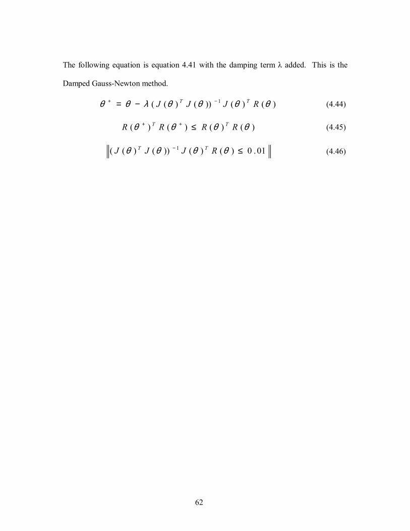
62
The following equation is equation 4.41 with the damping term λ added. This is the
Damped Gauss-Newton method.
)()())()(( 1 θθθθλθθ RJJJ TT −+ −= (4.44)
)()()()( θθθθ RRRR TT ≤++ (4.45)
01.0)()())()(( 1 ≤− θθθθ RJJJ TT (4.46)

63
CHAPTER 5
APPLICATION OF MATLAB® FUNCTIONS TO OBTAIN A FINITE ORDER TRANSFER FUNCTION OF A TOTAL FLUID
TRANSMISSION LINE SYSTEM 5.1 Total Fluid Transmission Line System
The hyperbolic transfer function matrix defines the input/output relationship of a
single fluid line. Typical hydraulic and pneumatic systems contain a number of fluid
lines and other resistive, inductive, and capacitive components.
Figure 5.1 Hydraulic brake valve schematic (Mico)
5.2 Application of Matlab® Symbolic Toolbox Commands to Model a Fluid Transmission Line
The following section provides example applications of Matlab® commands to
model a fluid transmission line system. Both a lumped and a distrubuted parameter

64
model are presented to illustrate the need to approximate the distributed parameter
model after the frequency domain transfer function is obtained.
5.2.1 Frequency and Time Response of Lumped Model
The Matlab® Symbolic Toolbox provides the �solve.m� program that will solve
an �n� number of symbolic equations for an �n� number of unknowns. For example, the
simple lumped parameter model for the blocked hydraulic transmission line discussed
earlier can be solved using the following command:
)Qin'Pout,',s'*Pout*CPQin',Qin'*s)*LI(RLPout-Pinsolve('Sol =+== (5.1)
Matlab® responds with the following output.
sym] [1x1 :Qin sym] [1x1 :Pout
Sol= (5.2)
To view the individual solution of Pout type:
Sol.PoutPout = (5.3)
Matlab® responds with the following output:
LI)*s^2*CPRL*s*CPPin/(1
Pout
++
= (5.4)
The input pressure value, Pin, needs to expressed as unity in order to obtain the
transfer function of the line rather than the particular solution. This can be
accomplished using the �subs� command to replace a symbolic term with a real value.
,1)Pin''subs(Pout,TF = (5.5)

65
LI)*s^2*CPRL*s*CP1/(1
TF
++
= (5.6)
An optional command can be used to make the solution in a typeset form.
.TF)pretty(Sol (5.7)
LI s CP RL s CP 1 ----------------------------------
1
2++
(5.8)
The present form of the solution is symbolic and needs to be converted in a form
that Matlab® can process. The �subs� command is used to replace all the symbolic
elements with actual values. Before the �subs� command can be run the values for each
symbolic parameter must already be in the Matlab® workspace.
;1Pind^4);*L)/(pi*p*Vis*(128RL
V/Be;CPr^2);*L)/(pi*(pLI
r^2;*pi*LVd/2;r0.01;d2;L
Bl); Bl)/(Bf * (Bf Be 1.73e7;Bl
1.21e9;Bf 5;-4.6eVis
870;p
===
==
===
+====
=
(5.9)
Note: all parameters are derived from metric units (m, Kg, and s).

66
RL),RL''subs(TF, TFCP),CP''subs(TF, TF
LI),LI''subs(TF, TF
===
(5.10)
Matlab® will return the solution in whole number form.
s^2)*04307229758825357311448411166153499415/...917437929122743915163390064782
...+s*4019206099265847069655257103845937127/...742001426964924424753118859599+1/(1= TF
(5.11)
This can be cleaned up using the �vpa� command to convert the rational whole
number expressions to decimal form and the symbolic propagation operator can be
replaced with this result using the �subs� command.
vpa(TF,5)TF = (5.12)
s^2)*3-.20403e+s*2-.30034e+1/(1.= TF (5.13)
This result cannot be processed by Matlab® commands designed for transfer
functions such as the �step� and �bode� commands. One reason for this is that the
Laplace operator in this result is symbolic. This can be converted to a Matlab® transfer
function by performing the following operations.
Den)tf(Num,TF1] 3-0.20403e 2-0.30034e[Den
1][Num
===
(5.14)
This produces the following output in the Matlab® workspace command line.

67
1 + s 0.003003 + s^2 0.000204-----------------------------
1 :functionTransfer
(5.15)
This result can be processed by the commands �bode� and �step� to produce the
frequency response and time domain response respectively.
bode(TF) (5.16)
step(TF) (5.17)
The natural frequency can be obtained from the characteristic equation of the second
order RLC model as follows:
22 2 nnn ss ωως ++ (5.18)
LCs
LRs 12 ++ (5.19)
701 ==LCnω (5.20)

68
Frequency (rad/sec)
Phas
e (d
eg)
Mag
nitu
de (d
B)
-60
-40
-20
0
20
101
102
103
-180
-135
-90
-45
0
ωn = 70
Figure 5.2 Frequency response plot of lumped parameter model
Time (sec)
Am
plitu
de
0 0.1 0.2 0.3 0.4 0.5 0.6 0.7 0.80
0.2
0.4
0.6
0.8
1
1.2
1.4
1.6
1.8
Figure 5.3 Time domain step input response plot of lumped parameter model

69
5.2.2 Frequency and Time Response of the Dissipative Model
This approach can also be applied to the more complex dissipative model. One
major advantage of this approach is that the causality does not need to be considered as
in the modal approximation method. The following symbolic equations can always be
used to define the line dynamics.
Distributed Parameter Line Equations
Pout*C21-Pin*C11=Qin (5.21)
Pout*C11-Pin*C21=Qout (5.22)
Distributed Parameter Transfer Functions, C1 and C2
sinh(G))*cosh(G)/(Z=C1 (5.23)
sinh(G))*1/(Z=C2 (5.24)
Impedance Constant, Z0
Bsigma))*1)-(v+sqrt(1*B)-Z0/(sqrt(1=Z (5.25)
Normalized Propagation Operator, Γ
B))-Bsigma)/(1*1)-(v+sqrt((1*s*Dn=G (5.26)
Unnormalized Propagation Operator, Γ
B))-Bsigma)/(1*1)-(v+sqrt((1*(r^2)/Vis)*(s*Dn=G (5.27)
Normalized Bessel Function Ratio with Prandtl Number, Brσ
s)))*sqrt(sigma*jbesselj(0,*s)*sqrt(sigma*(j s))/...*sqrt(sigma*jbesselj(1,*2=Bsigma (5.28)
Unnormalized Bessel Function Ratio with Prandtl Number, Brσ

70
)))(r^2)/Vis)*(s*sqrt(sigma*jbesselj(0, ...*)(r^2)/Vis)*(s*sqrt(sigma*(j
))/...(r^2)/Vis)*(s*sqrt(sigma*jbesselj(1,*2=Bsigma (5.29)
Normalized and Unnormalized Bessel Function Ratio, Br
sqrt(s)))*jbesselj(0,*sqrt(s)*jsqrt(s))/(*jbesselj(1,*2=B (5.30)
)))(r^2)/Vis)*sqrt((s*jbesselj(0,*)(r^2)/Vis)*sqrt((s*(j))/...(r^2)/Vis)*sqrt((s*jbesselj(1,*2=B (5.31)
The two dissipative line equations can be solved as follows using the �solve� command
to obtain a symbolic solution for the transfer function.
)Pout'Qin,',Pout'*C11-C21='0,Pout'*C21-C11=Qinsolve('=Sol (5.32)
As in the lumped parameter model, the input pressure value, Pin, is expressed as unity in
order to obtain the transfer function of the line rather than the particular solution.
The solve command provides the following symbolic solution for the transfer function.
C21/C11= TF (5.33)
The next step is to replace the symbolic terms by actual numeric values using the �subs�
command. This requires that the numeric values for C11 and C21 already exist in the
Matlab® workspace.
C21),C21''subs(TF,=TF (5.34)
C11),C11''subs(TF,=TF (5.35)
If the propagation operator, Γ, is treated as a symbol, the result is the familiar
distributed parameter transfer function for a blocked line, 1/cosh Γ. The computation of
the propagation operator produces a rather complex result.

71
(1/2)(1/2))))^s^*(1/2)8250230^1357680363...*478127875/1697100451073741824besseli(0,
(1/2)/...(1/2)/s^8250230^1357680363*(1/2))s^*(1/2)...8250230^1357680363*781278751697100454/...1073741824besseli(1,*82425/1073741-(1/(1*s...*319687542751136956040832/426060337502
G =
(5.36)
This can be cleaned up using the �vpa� command and the symbolic propagation operator
can be replaced with this result using the �subs� command.
(1/2)(1/2))))^s^*,.73721/besseli(0(1/2)...(1/2))/s^s^*,.73721besseli(1.*2.7129-(1/(1.*s*1-.14284e
=G (5.37)
(1/2))(1/2))))^s^*.73721besseli(0,(1/2)/...(1/2))/s^s^*,.73721besseli(1.*2.7129-(1/(1.*s*1-284e1/cosh(.14
= TF
(5.38)
It is important to mention that not only is this result not a convenient rational
polynomial form but also that this form is not recognized as a transfer function by
Matlab®. This result cannot be processed by Matlab® commands designed for transfer
functions such as the �step� and �bode� commands. The Laplace operator in this result
is symbolic and needs to be replaced by jω which must be an array of a specified
frequency range. A range of 1:10,000 is usually sufficient to cover all significant modes
of the response.
0000]1:[1w = (5.39)
w)*j,s''subs(TF,TFfreqs = (5.40)

72
The result is 10,000 data points that can now be graphed using the following
commands.
TFfreqs))log10(abs(*20TFmag = (5.41)
180/pi*eqs)angle(TFfrTFphase = (5.42)
);Decibels'ylabel(');rad/sec'Frequency xlabel('
);Plot' Magnitudetitle('TFmag),semilogx(w
);Plot'Magnitude',Name'figure(' g =
(5.43)
);Degrees'ylabel(');rad/sec'Frequency xlabel(');Plot' Phasetitle('
TFphase),semilogx(w);Plot' Phase',Name'figure(' h =
(5.44)
100 101 102 103 104-10
-5
0
5
10
15
20
Frequency rad/sec
Dec
ibel
s
Figure 5.4 Frequency magnitude response of dissipative model

73
100
101
102
103
104-200
-150
-100
-50
0
50
100
150
200
Frequency rad/sec
Deg
rees
Figure 5.5 Frequency response phase plot of dissipative model
The complex transfer function needs to be processed by the �invfreqs� command
to produce a rational polynomial transfer function. By inspection of the frequency
response graph, the appropriate order can be determined for the desired frequency
range.

74
100
101
102
103
104-10
-5
0
5
10
15
20
Frequency rad/sec
Dec
ibel
s
1st Mode
ω = 1000
2nd
3rd 4th
5th
Figure 5.6 Determination of required number of modes
In this example the frequency range to be analyzed is 1000 rad/sec. This
requires the rational polynomial approximation to contain five 2nd order modes.
1000]:[1wa = (5.45)
Here the exact solution needs to be scaled back from 10,000 rad/sec to 1,000 rad/sec in
order to be processed by the �invfreqs� command.
wa)*j,s''subs(TF,=TFfreqswa (5.46)

75
Since there are five 2nd order modes, a 10th order characteristic equation needs to
used. The numerator should be one order less than the denominator to produce a stable
transfer function.
wa,9,10)Ffreqswa,invfreqs(T=Den][Num, (5.47)
Den)tf(Num,=TFA (5.48)
1.814e026 s7.076e023s^21.696e022s^3 1.904e019 s^4 2.511e017
1.444e014 s^6 1.141e012 s^7 3.435e008 s^8 1.891e006 s^9 241.2 s^10
----------------------------------------------------------------------------------------
2.952e026 s 1.346e024 - s^2 6.89e021 s^3 2.792e019 - s^4 6.554e016
... s^5 1.437e014 - s^6 1.592e011 s^7 2.618e008 - s^8 1.354e005 s^9 160.3
:functionTransfer
++++
+++++
++
+++
(5.49)
The following commands are used to obtain the frequency response of the
approximate rational polynomial transfer function and plot a comparison graph with the
frequency response of the exact solution.
w)Den,freqs(Num,=TFAfreqs (5.50)
TFAfreqs))log10(abs(*20=TFAmag (5.51)
TFfreqs))log10(abs(*20=TFmag (5.52)
);Decibels'ylabel(');rad/sec'Frequency xlabel('
);Plot' Magnitudetitle(');r''TFAmag,w,,b''TFmag,,semilogx(w
);Plot'Magnitude',Name'figure(' = g
(5.53)

76
Figure 5.7 Frequency magnitude response of approximation without fit-error weighting
This result accurately models the exact response at the high frequencies but fails
at the low end of the frequency range. The gain of the approximation is also very
inaccurate. The �invfreqs� command can be modified to allow fit-errors to be weighted
verses frequency.
wt,100);wa,9,10,Ffreqs,invfreqs(T=Den][Num, (5.54)

77
Figure 5.8 Frequency magnitude response of approximation with fit-error weighting
This result almost exactly models the exact solution out to 1000 rad/sec. The
steady state gain of the approximation should be unity. The frequency magnitude
response curve shows a small error. The gain can be calculated with the following
command.
)dcgain(TFA=Gain (5.55)
0267231.04894105 =Gain (5.56)
The approximated transfer function can be divided by this amount to achieve a steady
state gain of unity.

78
Figure 5.9 Frequency magnitude response of approximation with normalized gain
Setting the steady state gain to unity resulted in a small increase in error of the
response at higher frequencies. Figure 5.10 shows the comparison magnitude and phase
plots of modal approximations using �invfreqs� where the maximum frequency for each
mode is the resonant frequency of the respective mode.

79
Figure 5.10 Frequency response of approximation with normalized gain for the first five modes

80
These approximations more accurately model the exact solution than the modal
approached covered in Chapter 3. A more accurate approximation can be achieved by
increasing the order of each mode by a factor of one. The drawback is that the transfer
function is of higher order, which is contrary to the objective of order reduction.
100
101
102
103
104-50
-40
-30
-20
-10
0
10
20
Frequency rad/sec
Dec
ibel
s
3rd Order5th 7th9
th11th
Figure 5.11 Frequency magnitude response of approximation using additional order for each mode

81
100
101
102
103
104-200
-150
-100
-50
0
50
100
150
200
Frequency rad/sec
Deg
rees
3rd Order
5th
7th
9th
11th
Figure 5.12 Frequency phase response of approximation using additional order for each mode
Time (sec)
Am
plitu
de
0 0.1 0.2 0.3 0.4 0.5 0.6-0.5
0
0.5
1
1.5
2
Figure 5.13 Step input response of modal approximations using �invfreqs�

82
As expected, a step input to each model does not result in much variation in the
time domain response, but an impulse input results in significant variation in the. This
illustrates the importance of having a model that is accurate in the frequency range that
the system operates.
Figure 5.14 Impulse input response of modal approximations using �invfreqs�
The goal of obtaining a finite order rational polynomial transfer function that
accurately models that exact solution has been accomplished. Now the result can be
implemented with other block elements to model a total system using classical control
theory methods. An even better approach is to use the �solve� command and �invfreqs�
to obtain an approximated transfer function for the total system.

83
5.3 Application of Matlab® Symbolic Toolbox Commands to Model a Total Fluid Transmission Line System
The �solve� command can provide symbolic solutions for problems with any
number of unknowns. In the following hydraulic brake system, there are seven
transmission lines, four capacitive elements, and one resistive element.
Figure 5.15 Multiple line system with capacitive and resistive elements
Each line is modeled with two equations for a total of 14 dissipative equations.
There is three summation equations where lines are joined. Resistive and Capacitive
Elements are modeled as lumped elements in the total system. This system is defined
by a total of 22 equations. The �solve� command is as follows:

84
)P27'P26,P25,P24,Ps3,Ps2,Ps1,P11,Q27...Q17,Q26,Q16,Q25,Q15,Q24,Q14,Q23,Q13,Q22,Q12,Q21,Q11,'
,...Q17'+Q16=Q23',Q15'+Q14=Q22',Q13'+Q12=Q21',...s'*P27*Cp7=Q27',s'*P26*Cp6=Q26',...s'*P25*Cp5=Q25',s'*P24*Cp4=Q24'
,...P27'*C17-Ps3*C27=Q27',P27'*C27-Ps3*C17=Q17',...P26'*C16-Ps3*C26=Q26',P26'*C26-Ps3*C16=Q16',...P25'*C15-Ps2*C25=Q25',P25'*C25-Ps2*C15=Q15',...P24'*C14-Ps2*C24=Q24',P24'*C24-Ps2*C14=Q14'
,...Ps3'*C13-Ps1*C23=Q23',Ps3'*C23-Ps1*C13=Q13',...Ps2'*C12-Ps1*C22=Q22',Ps2'*C22-Ps1*C12=Q12',...Ps1'*C11-P11*C21=Q21',Ps1'*C21-P11*C11=Q11'
,...Q11'*Rin=P11-solve('1=Sol
(5.57)
The individual solutions (symbolic and numeric) contain too many terms to
attempt to document. The following figures are the magnitude and phase plots for the
pressure output of line number 7.

85
100
101
102
103
104-60
-50
-40
-30
-20
-10
0
10
Frequency rad/sec
Dec
ibel
s
100
101
102
103
104-200
-150
-100
-50
0
50
100
150
200
Frequency rad/sec
Deg
rees
Figure 5.16 Frequency response plots for seven line brake system

86
100
101
102
103
104-70
-60
-50
-40
-30
-20
-10
0
10
Frequency rad/sec
Dec
ibel
s
3rd Order5th 7th
9th
11th
100
101
102
103
104-200
-150
-100
-50
0
50
100
150
200
Frequency rad/sec
Deg
rees
3rd Order
5th
7th
9th
11th
Figure 5.17 Frequency response modal approximation plots for seven line brake system

87
Time (sec)
Am
plitu
de
0 0.05 0.1 0.15 0.2 0.25 0.3 0.35 0.4-0.2
0
0.2
0.4
0.6
0.8
1
1.2
Figure 5.18 Step response modal approximation plot for seven line brake system
Time (sec)
Am
plitu
de
0 0.05 0.1 0.15 0.2 0.25 0.3 0.35 0.4-20
-10
0
10
20
30
40
50
60
Figure 5.19 Impulse response modal approximation plot for seven line brake system

88
The advantage of combining the total system in �solve� is that the order of the
system transfer function for a given frequency range will be reduced. If this is not
possible then the resulting transfer function must be combined in the classical method
with transfer functions of the remaining system components.
5.4 Application of Matlab® Matrix Commands to Model a Total Fluid Transmission
Line System
Another method of solving the system equations is to use a matrix. In this
approach, the only symbolic term is the Laplace operator.
= XAB (5.58)
=
P27
P26
P25
P24
Ps3
Ps2
Ps1
P11
Q27
Q17
Q26
Q16
Q25
Q15
Q24
Q14
Q23
Q13
Q22
Q12
Q21
Q11
0000000001-01-0000100000
00000000000001-01-001000
000000000000000001-01-10
s*Cp-000000010000000000000
0s*Cp-00000000100000000000
00s*Cp-0000000001000000000
000s*Cp-000000000010000000
C1(7)C2(7)-00000010000000000000
C2(7)C1(7)-00000001000000000000
0C1(6)C2(6)-0000000100000000000
0C2(6)C1(6)-0000000010000000000
00C1(5)C2(5)-000000001000000000
00C2(5)C1(5)-000000000100000000
000C1(4)C2(4)-00000000010000000
000C2(4)C1(4)-00000000001000000
0000C1(3)C2(3)-0000000000100000
0000C2(3)C1(3)-0000000000010000
00000C1(2)C2(2)-000000000001000
00000C2(2)C1(2)-000000000000100
000000C1(1)C2(1)-00000000000010
000000C2(1)C1(1)-00000000000001
000000010000000000000
0000000000000000000001 Rin
(5.59)

89
The following Matlab® command solves this equation using Gaussian Elimination.
BAX \= (5.60)
5.5 Application of Matlab® Graphical User Interface to Produce the Fluid
Transmission System Analyzer
The Matlab® tools previously covered have been incorporated into a Graphical
User Interface program that simplifies the process of obtaining a transfer function of a
fluid transmission line system. This program is prompted by inputting �FLRAR1� in the
Matlab® command line. The Graphical User Interface initially appears as follows:
Figure 5.20 GUI opening screen shot
The first thing required is to input the material constants of the fluid and the line
in the upper left corner as in the following example.

90
Note: all parameters are derived from metric units (m, kg, and s).
Figure 5.21 GUI material constants section
Figure 5.22 GUI model properties section
After completing the Model Properties section, the Model Diagram section will
automatically illustrate the model with a line diagram as shown here.

91
Figure 5.23 GUI model diagram section
The individual line lengths are specified in the Line Lengths section.
Figure 5.24 GUI line lengths section
The program will place the word �OUTPUT� above the lines that are output
lines. The input valve resistance, the output valve resistance and output capacitance
values are then placed in the following fields.
Figure 5.25 GUI line lengths section

92
Rout and CPout is restricted to the same values for all outputs. The program is
now ready to calculate the frequency response of the system using the Dissipative line
model. Click on the Frequency Response Analysis button to calculate the frequency
response.
Figure 5.26 GUI system solution section before analysis
The program uses the following algorithm to determine the modal frequencies.
a=0 for m=1 for k=1:9990 if TFmag(k+1) >= TFmag(k) if TFmag(k+1) >= TFmag(k+2) MF(m)= w(k+1) m=m+1 end end a=a+1 end end
(5.61)

93
Figure 5.27 GUI system solution section after analysis
Occasionally the algorithm fails to match mode to frequency, and a manual
override is necessary. The algorithm fails when modes do not have a local maximum
point. The manual frequency input can be determined by inspecting the frequency
magnitude response plot. The Upper Frequency value automatically shows after
selecting the number of modes. Finally, the Run Configuration button is pushed to
calculate the modal approximation and plot the approximated response against the exact
response.

94
Figure 5.28 GUI frequency response comparison output
The transfer function is displayed in the Matlab® command line.

95
(5.62)
The file can also be saved and loaded as needed. This command only saves the
solution parameters. The Frequency Response Analysis button needs to be pushed after
opening the file.
Figure 5.29 GUI complete screen shot

96
Figure 5.30 GUI layout editor screen shot
Figure 5.31 GUI files

97
5.6 Fluid Transmission System Analyzer Frequency Selection Application
A frequency response may be obtained that does not have modal frequencies
defined by a local maxima. The following figure is the result of a five mode
approximation of the same seven line system covered in the previous section. The
program fails to produce a perfect curve fit because the incorrect modal frequency is
selected by the program.
Figure 5.32 Failure of frequency determination algorithm
The frequency selected for the fifth mode is 566 rad/sec. By inspection of the
plot this is the frequency of the sixth mode. The problem in this example is the fourth
mode does not have a local maxima. In cases like this the Frequency Override feature

98
must be used. A frequency of 425 rad/sec is determined by visual inspection and
entered into the Frequency Override field and the configuration is rerun to produce the
following approximation.
Figure 5.33 Accurate approximation using frequency override

99
CHAPTER 6
SUMMARY OF RESEARCH AND RECOMMENDATION FOR FUTURE STUDY
6.1 Summary of Research
This research presents a method of solving for a total fluid transmission line
system using the dissipative model and then applying the Matlab® �invfreqs� algorithm
to the frequency response of the total system rather than individual lines. This can be
accomplished using the symbolic �solve� command or by matrix operations using a
symbolic Laplace operator. The advantage of this is apparent when there are several
lines in the system. Previously each line would be approximated in the Laplace domain
and the linear transfer functions lumped together. In this research, one approximation is
made on the total system rather than combining several approximations eliminating
combined error.
In addition to efficiently combining multiple fluid lines all the elements can be
combined before performing a modal approximation. Lumped resistive and capacitive
components as well as higher order elements can be combined with the lines and solved
for the frequency response of a particular output. Any element in the system can be
nonlinear. The only requirement is that the element is represented in the Laplace
domain.
An algorithm for matching mode to frequency is also introduced and all the tools
presented in this work are combined into a single user friendly program using the

100
Matlab® Graphical User Interface. This program provides an efficient method to
analyze a fluid transmission line system. To obtain a copy of the program send an
email request to: [email protected].
6.2 Recommendation for Future Study
The modifications made to the modal solution provided by �invfreqs� was to
normalize the transfer function to produce a steady state gain of unity and to increase
the order of the total number of modes by one. Improving the accuracy of the
approximation process so that the additional order can be reduced would be a major
improvement. The algorithm to determine modal frequency is based on the local
maxima of the frequency magnitude response. Occasionally, the modal frequency is not
defined by a local maxima and a manual determination of the frequency needs to be
made. Perhaps and algorithm based on inflection points would perform better. The
phase plot appears to have distinct inflection points.
The Matlab® features applied in this work are only a few of the tools available to
compute and analyze system models. One suggestion would be to produce a graphical
user interface that permits the inclusion of all system components. The program
introduced in this work is limited to multiple connected lines, an input resistive element
and output resistive and capacitive elements. A more comprehensive program should
be more flexible to allow for the input of all components of the system. Another
approach would be to find a method to automatically input a transfer function into
Matlab® Simulink and integrate this feature into an analysis program.

101
APPENDIX A
MODEL COMPARISON PROGRAM

102
The following Matlab® program plots a comparative frequency response of each of the
five models.
function system = MODELCOMP syms s %%%%%%%%%%%%%%%Model Properties%%%%%%%%%%%%%%%%%%%% p=870; Vis=4.6e-5; sigma=1; v=1; Bf=1.21e9; Bl=1.73e7; L=2; d=0.01; r=d/2; V=L*pi*r^2; w=[1:1000]; Pin=5e6; Be = (Bf * Bl)/(Bf + Bl) c=sqrt(Be/p) Dn=(Vis*L/(c*r^2)) wc=c/L; wv=Vis/r^2; %%%%%%%%Model 1: Lumped Parameter Model Calculation%%%%%%%%%%% LI=(p*L)/(pi*r^2) CP=V/Be RL=(128*Vis*p*L)/(pi*d^4) Sol=solve('Pin-Pout=(RL+LI*s)*Qin','Qin=CP*Pout*s','Pout,Qin') Pout=Sol.Pout TFM1=Pout TFM1=subs(TFM1,'LI',LI); TFM1=subs(TFM1,'CP',CP); TFM1=subs(TFM1,'RL',RL); TFM1=subs(TFM1,'wv',wv); TFM1=subs(TFM1,'Pin',Pin); TFM1=subs(TFM1,'s',j*w); TFM1MAG=20*log10(abs(TFM1));

103
%%%%%%%%%%%%%Model 2: Lossless Line Model Calculation%%%%%%%%%% G2=L*s/c; TFM2=Pin/cosh(G2); TFM2=subs(TFM2,'s',j*w); TFM2MAG=20*log10(abs(TFM2)); TFM2PHASE=angle(TFM2)*180/pi; %%%%%%%%%%%Model 3: Linear Friction Model Calculation%%%%%%%%%%% G3=((s/wc))*sqrt(1+(8*wv/(s))); TFM3=Pin/cosh(G3); TFM3=subs(TFM3,'s',j*w); TFM3MAG=20*log10(abs(TFM3)); TFM3PHASE=angle(TFM3)*180/pi; %%%%%%%%%%Model 4: Viscous Model Calculation%%%%%%%%%%%%%%%% B=1/sqrt(1-(2*besselj(1,j*sqrt((s/wv)))/(j*sqrt((s/wv))*besselj(0,j*sqrt((s/wv)))))); G4=B*s/wc; TFM4=Pin/cosh(G4); TFM4=subs(TFM4,'s',j*w); TFM4MAG=20*log10(abs(TFM4)); TFM4PHASE=angle(TFM4)*180/pi; %%%%%%%%%%%Model 5: Dissipative Model Calculation%%%%%%%%%%%%%%%%%%%% Bsigma=2*besselj(1,j*sqrt(sigma*(s/wv)))/(j*sqrt(sigma*(s/wv))*besselj(0,j*sqrt(sigma*(s/wv)))); B=2*besselj(1,j*sqrt((s/wv)))/(j*sqrt((s/wv))*besselj(0,j*sqrt((s/wv)))); G5=Dn*(s/wv)*sqrt((1+(v-1)*Bsigma)/(1-B)); TFM5=Pin/cosh(G5); TFM5=subs(TFM5,'s',j*w); TFM5MAG=20*log10(abs(TFM5)); TFM5PHASE=angle(TFM5)*180/pi; %%%%%%%%%%%Comparison Plot%%%%%%%%%%%%%%%%%%%%%% g = figure('Name','Magnitude Plot'); semilogx(w,TFM1MAG,w,TFM2MAG,w,TFM3MAG,w,TFM4MAG,w,TFM5MAG) title('Magnitude Plot'); xlabel('Frequency rad/sec'); ylabel('Decibels'); end

104
APPENDIX B
TRUNCATED PRODUCT SERIES MODAL APPROXIMATION PROGRAM
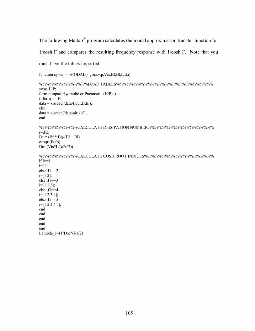
105
The following Matlab® program calculates the modal approximation transfer function for
1/cosh Γ and compares the resulting frequency response with 1/cosh Γ. Note that you
must have the tables imported.
function system = MODAL(sigma,v,p,Vis,Bf,Bl,L,d,i) %%%%%%%%%%%%%%LOAD TABLES%%%%%%%%%%%%%%%%%%%%%%%%%%%% syms H P; form = input('Hydraulic or Pneumatic (H/P):') if form == H data = xlsread('data-liquid.xls'); else data = xlsread('data-air.xls'); end %%%%%%%%%%%CALCULATE DISSIPATION NUMBER%%%%%%%%%%%%%%%%%%% r=d/2; Be = (Bf * Bl)/(Bf + Bl) c=sqrt(Be/p) Dn=(Vis*L/(c*r^2)) %%%%%%%%%%%CALCULATE COSH ROOT INDICES%%%%%%%%%%%%%%%%%%%% if i==1 i=[1]; else if i==2 i=[1 2]; else if i==3 i=[1 2 3]; else if i==4 i=[1 2 3 4]; else if i==5 i=[1 2 3 4 5]; end end end end end Lambda_c=(1/Dn)*(i-1/2)

106
%%%%%%%%%%%CALCULATE RESIDUE COEFFICIENTS%%%%%%%%%%%%%%%%%% DI = data(:,1); NF = data(:,2); DR = data(:,3); CA1 = data(:,4); CB1 = data(:,5); w = interp1(DI,NF,Lambda_c) d = interp1(DI,DR,Lambda_c) cosh_residue_a = interp1(DI,CA1,Lambda_c) cosh_residue_b = interp1(DI,CB1,Lambda_c) a = cosh_residue_a./(((-1).^(i+1)).*(1-2.*i)) b = cosh_residue_b./(((-1).^(i+1)).*(1-2.*i)) %%%%%%%%%% CALCULATE RATIONAL POLYNOMIAL APPROXIMATION %%%%%%%% Li=length(i); for k=1:Li num=[a(k) b(k)] den=[1 2*d(k)*w(k) w(k)^2] APPROXTF(k)=tf(num,den) k=k+1; end %%%%%%%%%%% EXACT MODEL CALCULATION %%%%%%%%%%%%%%%%%%%% w=[0.01:1000]; syms s Z0=(p*c)/(pi*r^2); Bsigma=2*besselj(1,j*sqrt(sigma*(s)))/(j*sqrt(sigma*(s))*besselj(0,j*sqrt(sigma*(s)))); B=2*besselj(1,j*sqrt((s)))/(j*sqrt((s))*besselj(0,j*sqrt((s)))); Z=Z0/(sqrt(1-B)*sqrt(1+(v-1)*Bsigma)); G=Dn*(s)*sqrt((1+(v-1)*Bsigma)/(1-B)); EXACT=1/cosh(G); EXACT=vpa(EXACT,5) EXACT=subs(EXACT,'s',j*w); EXACTMAG=20*log10(abs(EXACT)); EXACTPHASE=angle(EXACT)*180/pi; %%%%%%%%%%% MODAL COMPARISON TO EXACT %%%%%%%%%%%%%%%%%%% if length(i)==1 Gainsum1=dcgain(APPROXTF(1)); TFsum1=APPROXTF(1)/Gainsum1 [n1,d1] = tfdata(TFsum1,'v'); APPROX1=freqs(n1,d1,w); APPROXMAG1=20*log10(abs(APPROX1)); APPROXPHASE1=angle(APPROX1)*180/pi; g = figure('Name','Magnitude Plot');

107
semilogx(w,EXACTMAG,w,APPROXMAG1) title('Magnitude Plot'); xlabel('Normalized Frequency rad/sec'); ylabel('Decibels'); h = figure('Name','Phase Plot'); semilogx(w,EXACTPHASE,w,APPROXPHASE1) title('Phase Comparison Plots'); xlabel('Normalized Frequency rad/sec'); ylabel('Degrees'); elseif length(i)==2 Gainsum1=dcgain(APPROXTF(1)); TFsum1=APPROXTF(1)/Gainsum1; TFsum2=(APPROXTF(1)+APPROXTF(2)); Gainsum2=dcgain(TFsum2); TFsum2=TFsum2/Gainsum2; [n1,d1] = tfdata(TFsum1,'v'); [n2,d2] = tfdata(TFsum2,'v'); APPROX1=freqs(n1,d1,w); APPROX2=freqs(n2,d2,w); APPROXMAG1=20*log10(abs(APPROX1)); APPROXMAG2=20*log10(abs(APPROX2)); APPROXPHASE1=angle(APPROX1)*180/pi; APPROXPHASE2=angle(APPROX2)*180/pi; g = figure('Name','Magnitude Plot'); semilogx(w,EXACTMAG,w,APPROXMAG1,w,APPROXMAG2) title('Magnitude Plot'); xlabel('Normalized Frequency rad/sec'); ylabel('Decibels'); h = figure('Name','Phase Plot'); semilogx(w,EXACTPHASE,w,APPROXPHASE1,w,APPROXPHASE2) title('Phase Comparison Plots'); xlabel('Normalized Frequency rad/sec'); ylabel('Degrees'); elseif length(i)==3 Gainsum1=dcgain(APPROXTF(1)); TFsum1=APPROXTF(1)/Gainsum1 TFsum2=(APPROXTF(1)+APPROXTF(2)) Gainsum2=dcgain(TFsum2); TFsum2=TFsum2/Gainsum2 TFsum3=(APPROXTF(1)+APPROXTF(2)+APPROXTF(3)) Gainsum3=dcgain(TFsum3); TFsum3=TFsum3/Gainsum3 [n1,d1] = tfdata(TFsum1,'v');

108
[n2,d2] = tfdata(TFsum2,'v'); [n3,d3] = tfdata(TFsum3,'v'); APPROX1=freqs(n1,d1,w); APPROX2=freqs(n2,d2,w); APPROX3=freqs(n3,d3,w); APPROXMAG1=20*log10(abs(APPROX1)); APPROXMAG2=20*log10(abs(APPROX2)); APPROXMAG3=20*log10(abs(APPROX3)); APPROXPHASE1=angle(APPROX1)*180/pi; APPROXPHASE2=angle(APPROX2)*180/pi; APPROXPHASE3=angle(APPROX3)*180/pi; g = figure('Name','Magnitude Plot'); semilogx(w,EXACTMAG,w,APPROXMAG1,w,APPROXMAG2,w,APPROXMAG3) title('Magnitude Plot'); xlabel('Normalized Frequency rad/sec'); ylabel('Decibels'); h = figure('Name','Phase Plot'); semilogx(w,EXACTPHASE,w,APPROXPHASE1,w,APPROXPHASE2) title('Phase Comparison Plots'); xlabel('Normalized Frequency rad/sec'); ylabel('Degrees'); elseif length(i)==4 Gainsum1=dcgain(APPROXTF(1)); TFsum1=APPROXTF(1)/Gainsum1 TFsum2=(APPROXTF(1)+APPROXTF(2)); Gainsum2=dcgain(TFsum2); TFsum2=TFsum2/Gainsum2 TFsum3=(APPROXTF(1)+APPROXTF(2)+APPROXTF(3)); Gainsum3=dcgain(TFsum3); TFsum3=TFsum3/Gainsum3 TFsum4=(APPROXTF(1)+APPROXTF(2)+APPROXTF(3)+APPROXTF(4)); Gainsum4=dcgain(TFsum4); TFsum4=TFsum4/Gainsum4 [n1,d1] = tfdata(TFsum1,'v'); [n2,d2] = tfdata(TFsum2,'v'); [n3,d3] = tfdata(TFsum3,'v'); [n4,d4] = tfdata(TFsum4,'v'); APPROX1=freqs(n1,d1,w); APPROX2=freqs(n2,d2,w); APPROX3=freqs(n3,d3,w); APPROX4=freqs(n4,d4,w); APPROXMAG1=20*log10(abs(APPROX1)); APPROXMAG2=20*log10(abs(APPROX2)); APPROXMAG3=20*log10(abs(APPROX3)); APPROXMAG4=20*log10(abs(APPROX4));

109
APPROXPHASE1=angle(APPROX1)*180/pi; APPROXPHASE2=angle(APPROX2)*180/pi; APPROXPHASE3=angle(APPROX3)*180/pi; APPROXPHASE4=angle(APPROX4)*180/pi; g = figure('Name','Magnitude Plot'); semilogx(w,EXACTMAG,w,APPROXMAG1,w,APPROXMAG2,w,APPROXMAG3,w,APPROXMAG4) title('Magnitude Plot'); xlabel('Normalized Frequency rad/sec'); ylabel('Decibels'); h = figure('Name','Phase Plot'); semilogx(w,EXACTPHASE,w,APPROXPHASE1,w,APPROXPHASE2,w,APPROXPHASE3,w,APPROXPHASE4) title('Phase Comparison Plots'); xlabel('Normalized Frequency rad/sec'); ylabel('Degrees'); end

110
APPENDIX C
�INVFREQS� MODAL APPROXIMATION COMPARISON PROGRAM

111
The following Matlab® program plots the frequency response of several modal
approximations of a given fluid line using the �invfreqs� command.
function system = MODALDISS warning off syms s %%%%%%%%%%%%%%%%%%%% Model Properties %%%%%%%%%%%%%%%%%%%% p=870; Vis=4.6e-5; Bf=1.21e9; Bl=1.73e7; L=2; d=0.01; r=d/2; V=L*pi*r^2; Be = (Bf * Bl)/(Bf + Bl); c=sqrt(Be/p); Dn=(Vis*L/(c*r^2)); sigma=1; v=1; %%%%%%%%%% Number of Modal Approximations to Plot %%%%%%%%%%%%%%%%%%% ModeNum=5 %%%%%%%%%%%%%%%%%%%%%%%% Exact %%%%%%%%%%%%%%%%%%%%%%% B=2*besselj(1,j*sqrt((s*(r^2)/Vis)))/(j*sqrt((s*(r^2)/Vis))*besselj(0,j*sqrt((s*(r^2)/Vis)))); Bsigma=2*besselj(1,j*sqrt(sigma*(s*(r^2)/Vis)))/(j*sqrt(sigma*(s*(r^2)/Vis))*besselj(0,j*sqrt(sigma*(s*(r^2)/Vis)))); Z0=(p*c)/(pi*r^2); Z=Z0/(sqrt(1-B)*sqrt(1+(v-1)*Bsigma)); G=Dn*(s*(r^2)/Vis)*sqrt((1+(v-1)*Bsigma)/(1-B)); w=[1:10000];

112
C11=cosh(G)/(Z*sinh(G)); C21=1/(Z*sinh(G)); Sol=solve('QIN=C11-C21*POUT','0=C21-C11*POUT','QIN,POUT'); TF=Sol.POUT; TF=subs(TF,'C11',C11); TF=subs(TF,'C21',C21); TFfreqs=subs(TF,'s',j*w); TFmag=20*log10(abs(TFfreqs)); TFphase=angle(TFfreqs)*180/pi; %%%%%%%%%%%%%%%%%%%Modal Frequency Range%%%%%%%%%%%%%%%%%%%% a=0; for m=1; for k=1:9990; if TFmag(k+1) >= TFmag(k); if TFmag(k+1) >= TFmag(k+2); Modefreqs(m)= w(k+1); m=m+1; end; end; a=a+1; end end %%%%%%%%%%%%%%%%%%%% Approximation Plots %%%%%%%%%%%%%%%%%%%% g = figure('Name','Magnitude Plot'); for m=1:ModeNum; Modefreqs(m); wa=[1:Modefreqs(m)]; TFfreqs=subs(TF,'s',j*wa); wt=ones(size(wa)); [Num,Den]=invfreqs(TFfreqs,wa,(2*m-1),(2*m),wt,100); TFA=tf(Num,Den); Gain=dcgain(TFA); TFA=TFA/Gain; [Num,Den] = tfdata(TFA,'v'); TFAfreqs=freqs(Num,Den,w); TFAmag=20*log10(abs(TFAfreqs)); semilogx(w,TFmag,'b',w,TFAmag,'r'); hold on title('Magnitude Plot'); xlabel('Frequency rad/sec'); ylabel('Decibels'); end hold off h = figure('Name','Phase Plot'); for m=1:5; Modefreqs(m); wa=[1:Modefreqs(m)];

113
TFfreqs=subs(TF,'s',j*wa); wt=ones(size(wa)); [Num,Den]=invfreqs(TFfreqs,wa,(2*m-1),(2*m),wt,100); TFA=tf(Num,Den); Gain=dcgain(TFA); TFA=TFA/Gain; [Num,Den] = tfdata(TFA,'v'); TFAfreqs=freqs(Num,Den,w); TFAphase=angle(TFAfreqs)*180/pi; semilogx(w,TFphase,'b',w,TFAphase,'r'); hold on title('Phase Plot'); xlabel('Frequency rad/sec'); ylabel('Degrees'); end

114
REFERENCES
[1] R.L. Woods and K.L. Lawrence, Modeling and Simulation of Dynamic Systems,
Prentice-Hall, 1997.
[2] R.C. Dorf and R.H. Bishop, Modern Control Systems, Prentice-Hall, 2001.
[3] J.M. Kirshner and Silas Katz, Design Theory of Fluidic Components,
Academic Press, Inc., 1975.
[4] Y.C. Fung, A First Course In Continuum Mechanics, Prentice-Hall, 1994.
[5] A.S. Iberall, Attenuation of oscillatory pressures in instrument lines. J. Res. Nat.
Bur. Stand. 45, Res. Paper 2115 (1950).
[6] C.R. Gerlach, �Dynamic Models for Viscous Fluid Transmission Lines,�
Proceedings of the 10th Joint Automatic Control Conference, Boulder,
Colorado, 1969.
[7] R.E. Goodson and R.G. Leonard, �A Survey of Modeling Technique for Fluid
Transmission Line Transients,� Journal of Basic Engineering, ASME
Transactions, Series D, Vol. 94, June 1972.
[8] R.L. Woods, �The Effects of Source and Load Impedance Connected to Fluid
Transmission Lines,� Fluid Transmission Lines Dynamics, ASME Special
Publication, New York, November 1981.

115
[9] P. Wongputorn, D.A. Hullender, and R.L. Woods, �Rational Polynomial
Transfer Function Approximations for Fluid Transcients in Line�. Proceedings
of FEDSM�03, 4th ASME_JSME Joint Fluids Engineering Conference,
Honolulu, Hawaii, USA, July 6-11, 2003.
[10] Karen Willcox, �Reduced Order Aerodynamic Models For Aeroelastic Control
of Turbomachines�. dissertation, Doctor of Philosophy, Massachusetts Institute
of Technology., February 2000.
[11] F.T. Brown, �The Transient Response of Fluid Lines�, Journal of Basic
Engineering, ASME Transactions, Series D, Vol. 84, No. 4, December 1962.
[12] F.T. Brown and S.E. Nelson, �Step Response of Fluid Lines with Frequency-
Dependent Effects of Viscosity�, Journal of Basic Engineering, ASME
Transactions, Series D, Vol. 89, No. 2, June 1965.
[13] D'Souza, A. F. and Oldenburger. R., �Dynamic Response of Fluid Lines�,
Journal of Basic Engineering, ASME Transactions, September 1964.
[14] D.A. Hullender and A.J. Healey, �Rational Polynomial Approximations for
Fluid Transmission Line Models,� Fluid Transmission Lines Dynamics, ASME
Special Publication, New York, November 1981.
[15] C.Y. Hsue and D.A. Hullender, �Modal Approximations for the Fluid Dynamics
of Hydraulic and Pneumatic Transmission Lines� Fluid Transmission Lines
Dynamics, ASME Special Publication, Vol. II, New York, November 1983.

116
[16] D.A. Hullender and R.L. Woods, �Time Domain Simulation of Fluid
Transmission Lines using Minimum Order State Variable Models� Fluid
Transmission Lines Dynamics, ASME Special Publication, Vol. II, New York,
November 1983.
[17] Witrisnanto Sih Nursilo, �Fluid Transmission Line Dynamics� dissertation,
Doctor of Philosophy, The University of Texas at Arlington, Arlington, Texas,
August 2000.
[18] P. Wongputorn, �Time Domain Simulation of Systems with Fluid Transmission
Lines� dissertation, Master of Science, The University of Texas at Arlington,
Arlington, Texas, August 2001.
[19] Howard Eves, An Introduction to the History of Mathematics, Saunders College
Publishing, 1990.
[20] Stanley I. Grossman, Elementary Linear Algebra, 3rd edition, Wadsworth
Publishing, 1987.
[21] The MathWorks Inc., Signal Processing Toolbox User�s Guide, Version 5,
Natick, Massachusetts, 1999.
[22] E.C. Levi, �Complex-Curve Fitting,� IRE Transactions on Automatic Control,
Vol. AC-4, pp. 37-44, May 1959.
[23] C.K. Sanathanan and J. Koerner, �Transfer Function Synthesis as a Ratio of
Two Complex Polynomials�, IRE Transactions on Automatic Control, Vol. AC-
8, pp. 56-58, January 1963.

117
BIOGRAPHICAL STATEMENT
John King was born in Janesville, Wisconsin in 1962. After high school he
joined the U.S. Air Force where he worked as a Target Intelligence Specialist at RAF
Upper Heyford, England. He received a Bachelor of Science in Mechanical
Engineering from the University of Texas at Arlington in 1993. He has worked in the
telecommunications industry since 1994 and has been Sales Engineer at Fujitsu
Network Communications, Inc. since 1998. He received his Master of Science in
Mechanical Engineering from the University of Texas at Arlington in May 2006. His
research interests are dynamic systems modeling and transmission line theory.