FREQUENCY-DOMAIN NUMERICAL BUFFETING RESPONSE …uet.vnu.edu.vn/~thle/Frequency-domain numerical...
23
1 | Le Thai Hoa – Frequency domain buffeting response prediction: II. Example FREQUENCY-DOMAIN NUMERICAL BUFFETING RESPONSE PREDICTION II. EXAMPLE Prepared by Le Thai Hoa 2004
Transcript of FREQUENCY-DOMAIN NUMERICAL BUFFETING RESPONSE …uet.vnu.edu.vn/~thle/Frequency-domain numerical...

1 | L e T h a i H o a – F r e q u e n c y d o m a i n b u f f e t i n g r e s p o n s e p r e d i c t i o n : I I . E x a m p l e
FREQUENCY-DOMAIN NUMERICAL BUFFETING RESPONSE PREDICTION
II. EXAMPLE
Prepared by Le Thai Hoa
2004

2 | L e T h a i H o a – F r e q u e n c y d o m a i n b u f f e t i n g r e s p o n s e p r e d i c t i o n : I I . E x a m p l e
FREQUENCY-DOMIAN NUMERICAL BUFFETING RESPONSE PREDICTION: II. EXAMPLE
1. ANALYTICAL PROCEDURES
Step-wise analytical procedure (1) Field wind parameter:
a) Mean wind velocity (U10 & Uz); wind directions
b) Turbulence intensities (Iu, Iw)
c) Correlation and correlation coefficient ()
d) Scales of Turbulence (Lux, L)
e) PSD (Su(n), Sw(n))
(2) Force coefficient parameters:
a) Static force coefficients (CL, CD, CM at zero angle attack 0 )
b) Slope of static force coefficient (d
dCC LL ' ;
ddCC D
D ' ; d
dCC MM ' )
C’L, C’D, C’M
(3) Correction functions and transfer function:
a) Aerodynamic admittance (|L(n)|2 , |D(n)|2 , |M(n)|2)
b) Coherence (|CohL(n,s)|2, |CohD(n,s)|2 , |CohM(n,s)|2
c) Joint acceptance function (|JL(n)|2, |JD(n)|2, |JM(n)|2
d) Mechanical admittance (|Hi(n)|2)
(4) Full-bridge analysis and free vibration characteristics:
a) Free vibration analysis: Modal value and frequencies
b) Modal integral sums
3 | L e T h a i H o a – F r e q u e n c y d o m a i n b u f f e t i n g r e s p o n s e p r e d i c t i o n : I I . E x a m p l e
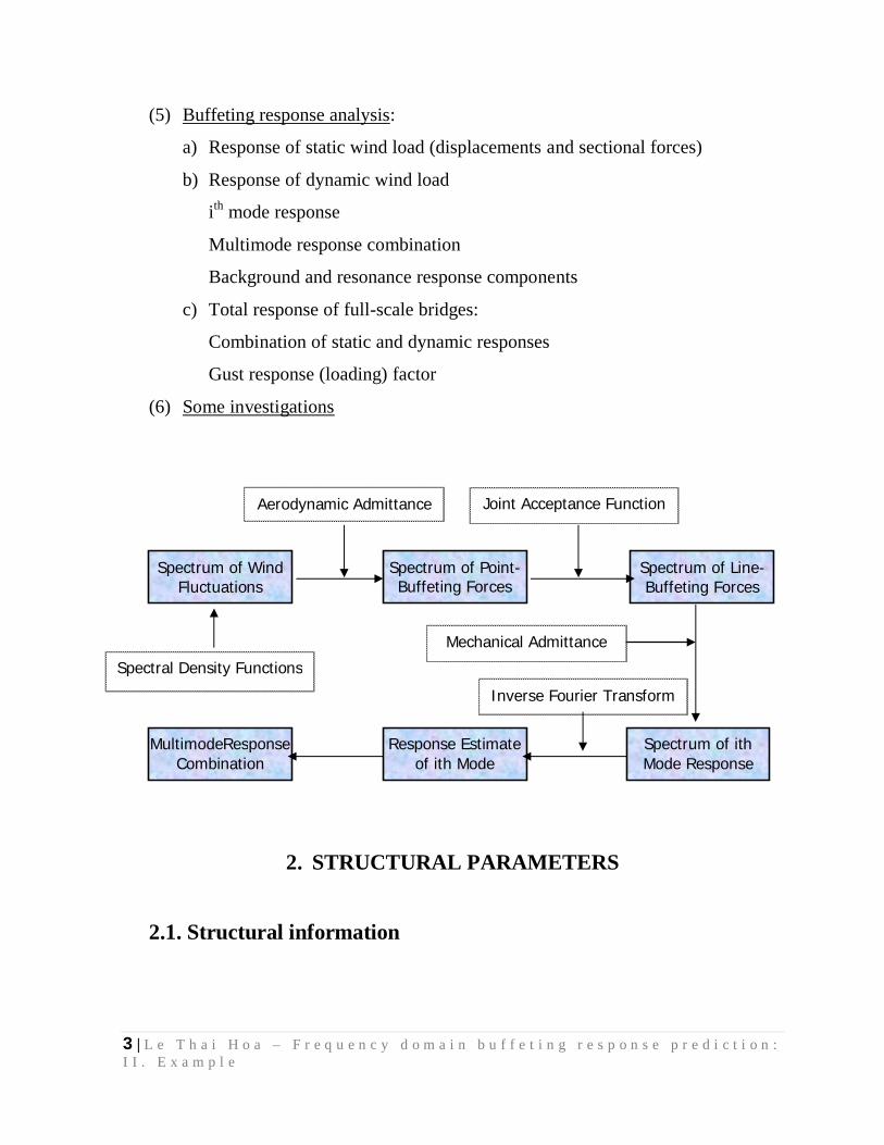
(5) Buffeting response analysis:
a) Response of static wind load (displacements and sectional forces)
b) Response of dynamic wind load
ith mode response
Multimode response combination
Background and resonance response components
c) Total response of full-scale bridges:
Combination of static and dynamic responses
Gust response (loading) factor
(6) Some investigations
2. STRUCTURAL PARAMETERS
2.1. Structural information
Spectrum of Wind Fluctuations
Spectrum of Point- Buffeting Forces
Spectrum of Line- Buffeting Forces
Spectrum of ith Mode Response
Response Estimate of ith Mode
Aerodynamic Admittance Joint Acceptance Function
Mechanical Admittance
Spectral Density Functions
MultimodeResponse Combination
Inverse Fourier Transform

4 | L e T h a i H o a – F r e q u e n c y d o m a i n b u f f e t i n g r e s p o n s e p r e d i c t i o n : I I . E x a m p l e
(1) A cable-stayed bridge example for numerical buffeting prediction (as model
of Diapoulsau Bridge, Swistherland) for demonstration of analytical
procedures and investigation
(2) Span arrangement: L=40.5m + 97m + 40.5m
2.2. Geometrical and material characteristics Gider Tower Stayed cables
Material parameters
E =3600000 T/m2
G =1384600 T/m2
=0.3 Poison ratio
Geometrical parameter
A =6.525 m2
I33 =0.11 m4
I22 =114.32 m4
J =0.44m4
Material parameters
E =3600000 T/m2
G =1384600 T/m2
=0.3 Poison ratio
Geometrical parameter
A =1.14 m2; I33=0.257 m4
I22 =0.118 m4;J=0.223m4
A =1.14 m2; I33=0.257 m4
I22 =0.118 m4;J=0.223m4
Material parameters
E = 19500000 T/m2
Geometrical parameter
A =26.355 cm2 Type 19K15
A =16.69 cm2 Type 12K15

5 | L e T h a i H o a – F r e q u e n c y d o m a i n b u f f e t i n g r e s p o n s e p r e d i c t i o n : I I . E x a m p l e
3. FREE VIBRATION ANALYSIS
AND MODAL INTEGRAL SUMS
3.1. Structural modelling and free vibration analysis (1) FEM’s 3D space frame model with single grillage of bridge deck has been
used for static and free vibration analyses. Nonlinearity due to cable sagging
has been taken into consideration as Ernst’s secant equivalent elastic
modulus in which innitial cable tenstion has been estimated thanks to deck-
elevated preshaping procedure. Structural analyses have been carried out by
computer-aided structural analysis package SAP2000 Nonlinear
(Computers&Structures 1998)
(2) Free vibration analysis based on the Eigenvector analysis (Modal analysis)
has determined undamped free-vibration mode shape and frequencies of the
system itself. 10 fundamental free modes and their charctericstics were
computed.
(3) Eigenvectors (or modal amplitudes) of each mode shapes have been
normalized (so-called the mass-matrix-based normalization or
transformation into the normalized coordinates) by the structural mass
matrix M as follows:
1iTi M
(4) The modal participataion factors are defined as participaed contributions of
masses and inertia moments of mass associated with the three global
coordinates X, Y, Z have been computed for each mode as:
dxxmf Xi
L
iXi )(0
x: spanwise coordinate
6 | L e T h a i H o a – F r e q u e n c y d o m a i n b u f f e t i n g r e s p o n s e p r e d i c t i o n : I I . E x a m p l e
dxxmf Yi
L
iYi )(0
dxxmf Zi
L
iZi )(0
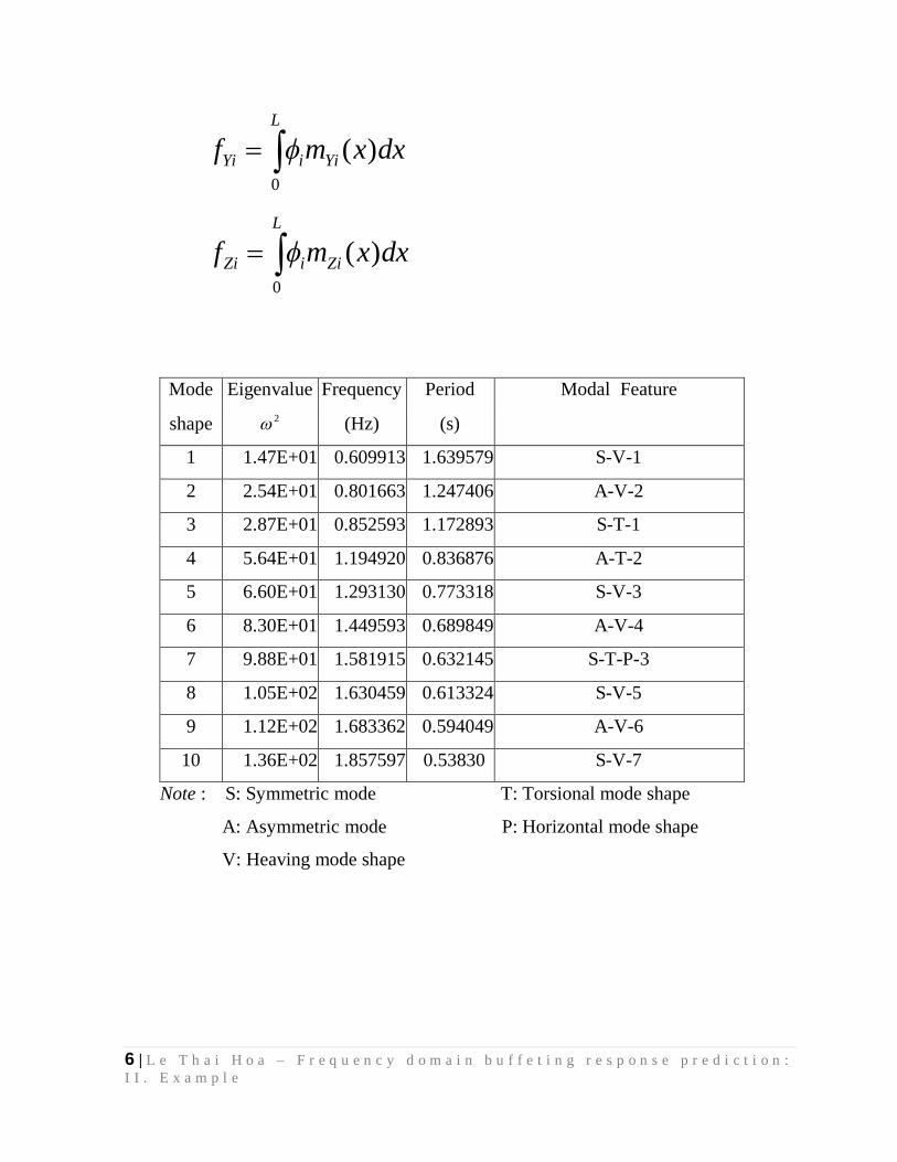
Mode Eigenvalue Frequency Period Modal Feature
shape 2 (Hz) (s)
1 1.47E+01 0.609913 1.639579 S-V-1
2 2.54E+01 0.801663 1.247406 A-V-2
3 2.87E+01 0.852593 1.172893 S-T-1
4 5.64E+01 1.194920 0.836876 A-T-2
5 6.60E+01 1.293130 0.773318 S-V-3
6 8.30E+01 1.449593 0.689849 A-V-4
7 9.88E+01 1.581915 0.632145 S-T-P-3
8 1.05E+02 1.630459 0.613324 S-V-5
9 1.12E+02 1.683362 0.594049 A-V-6
10 1.36E+02 1.857597 0.53830 S-V-7
Note : S: Symmetric mode T: Torsional mode shape
A: Asymmetric mode P: Horizontal mode shape
V: Heaving mode shape
7 | L e T h a i H o a – F r e q u e n c y d o m a i n b u f f e t i n g r e s p o n s e p r e d i c t i o n : I I . E x a m p l e
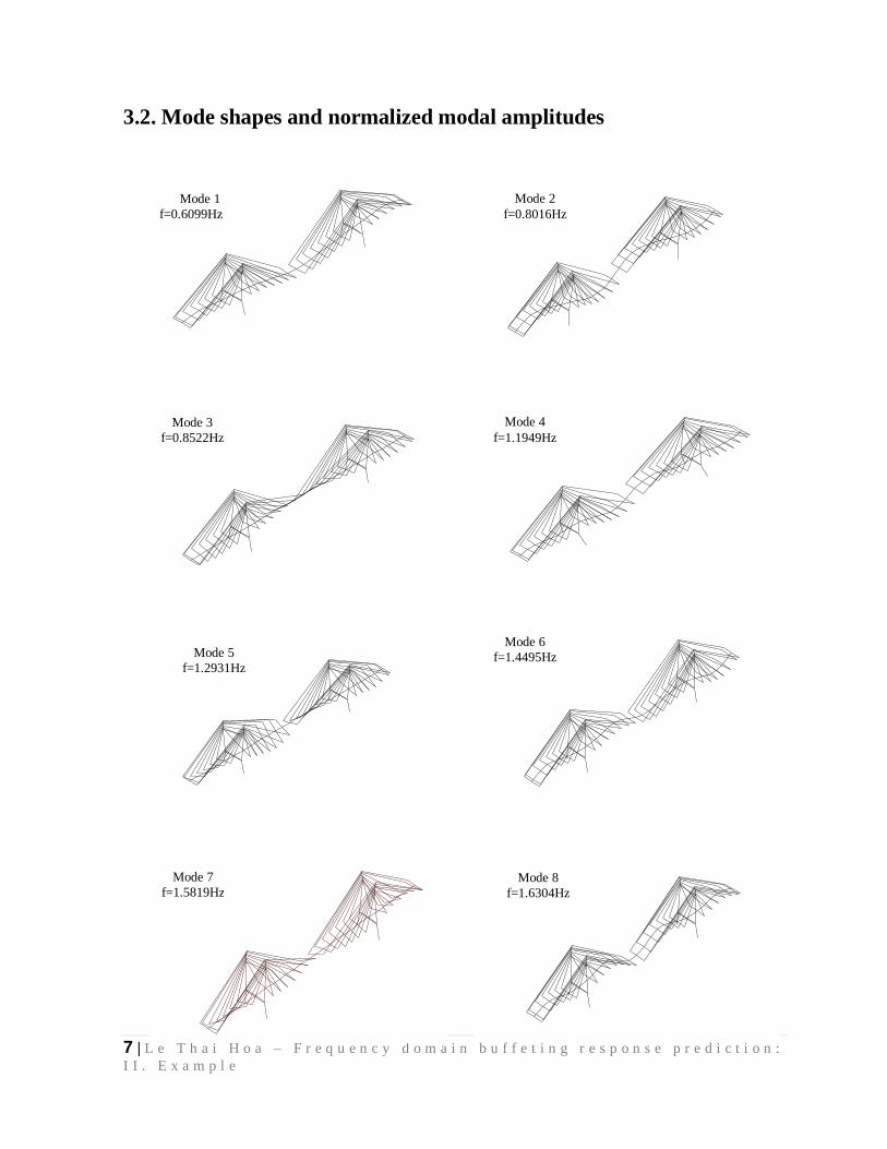
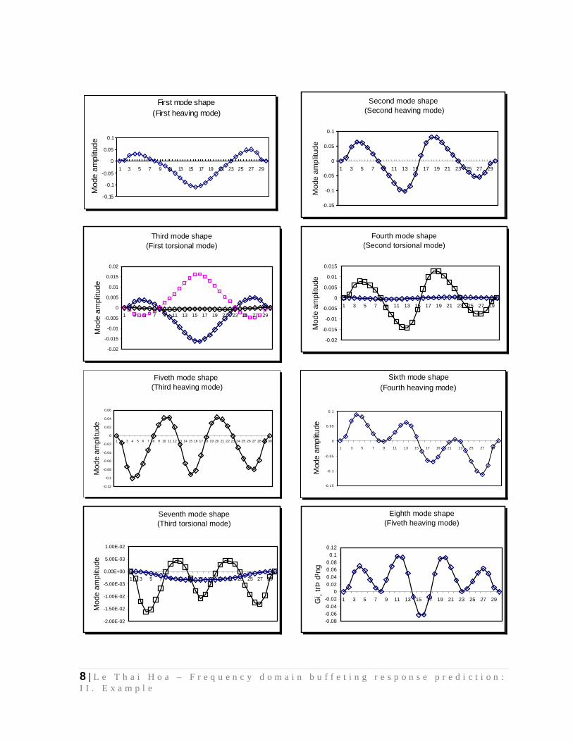
3.2. Mode shapes and normalized modal amplitudes
Mode 1 f=0.6099Hz
Mode 2 f=0.8016Hz
Mode 3 f=0.8522Hz
Mode 4 f=1.1949Hz
Mode 5 f=1.2931Hz
Mode 6 f=1.4495Hz
Mode 7 f=1.5819Hz
Mode 8 f=1.6304Hz
8 | L e T h a i H o a – F r e q u e n c y d o m a i n b u f f e t i n g r e s p o n s e p r e d i c t i o n : I I . E x a m p l e
Second mode shape
(Second heaving mode)
-0.15
-0.1
-0.05
0
0.05
0.1
1 3 5 7 9 11 13 15 17 19 21 23 25 27 29
Mod
e am
plitu
de
Third mode shape
(First torsional mode)
-0.02
-0.015
-0.01
-0.005
0
0.005
0.01
0.015
0.02
1 3 5 7 9 11 13 15 17 19 21 23 25 27 29
Mod
e am
plitu
de
Fourth mode shape(Second torsional mode)
-0.02
-0.015
-0.01
-0.005
0
0.005
0.01
0.015
1 3 5 7 9 11 13 15 17 19 21 23 25 27 29
Mod
e am
plitu
de
Fiveth mode shape (Third heaving mode)
-0.12
-0.1
-0.08
-0.06
-0.04
-0.02
0
0.02
0.04
0.06
1 2 3 4 5 6 7 8 9 10 11 12 13 14 15 16 17 18 19 20 21 22 23 24 25 26 27 28 29 30
Mod
e am
plitu
de
Sixth mode shape(Fourth heaving mode)
-0.15
-0. 1
-0.05
0
0.05
0. 1
1 3 5 7 9 11 13 15 17 19 21 23 25 27 29
Mod
e am
plitu
de
Seventh mode shape(Third torsional mode)
-2.00E-02
-1.50E-02
-1.00E-02
-5.00E-03
0.00E+00
5.00E-03
1.00E-02
1 3 5 7 9 11 13 15 17 19 21 23 25 27 29
Mod
e am
plitu
de
Eighth mode shape(Fiveth heaving mode)
-0.08-0.06-0.04-0.02
00.020.040.060.08
0.10.12
1 3 5 7 9 11 13 15 17 19 21 23 25 27 29Gi ̧
trÞ
d¹n
g
First mode shape (First heaving mode)
-0.15
-0.1
-0.05
0
0.05
0.1
1 3 5 7 9 11 13 15 17 19 21 23 25 27 29
Mod
e am
plitu
de

9 | L e T h a i H o a – F r e q u e n c y d o m a i n b u f f e t i n g r e s p o n s e p r e d i c t i o n : I I . E x a m p l e
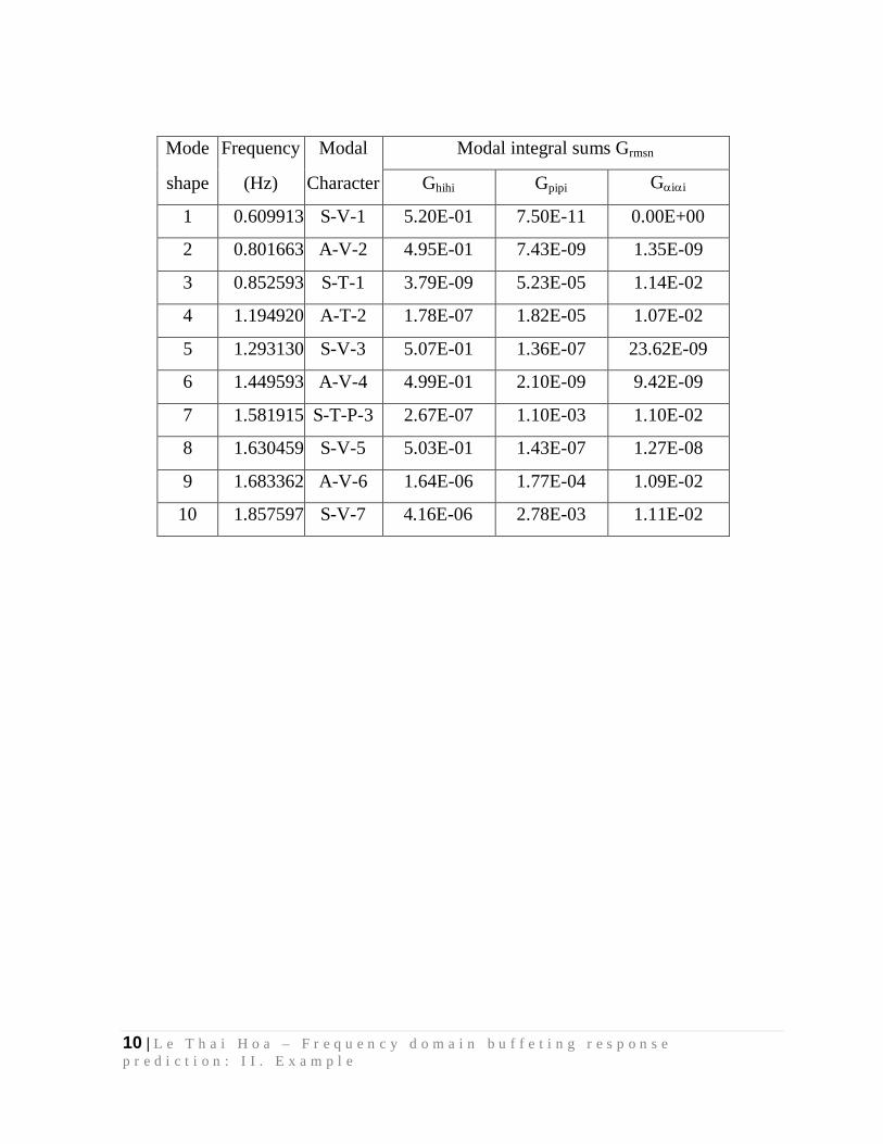
3.3. Modal integral sums Modal integral sums is considered as parameters to account to mode shapes and their
modal amplitude, modal spanwise distribution associated with any individual free
mode as well as coupling between modes. Modal intergral sums can be computed as
following formula:
L
kskrrmsn dxxxLG0
,, )().()( (x: spanwise direction)
N
knksmkrkrmsn LG
1,, )()(
(Unit: length unit as meter)
N: Number of deck nodes
Lk: Length interval between 2 nodes
k: Nodal indicator
r, s: Modal indicator
m, n: Combination indicator
r, s=h, p or : Heaving, lateral or rotational
m, n=i or j
mkr )( , : rth modal value at node k
rmrmG : Same modes and same coordinate (r=s, m=n); (Auto-modal sums)
rmsmG : Same modes and different coordinate (r#s, m=n); (Cross-modal sums)
rmrnG : Different modes and same coordinate (r=s, m#n)
rmsnG : Different modes and different coordinate (r#s, m#n)
10 | L e T h a i H o a – F r e q u e n c y d o m a i n b u f f e t i n g r e s p o n s e p r e d i c t i o n : I I . E x a m p l e
Mode Frequency Modal Modal integral sums Grmsn
shape (Hz) Character Ghihi Gpipi Gii
1 0.609913 S-V-1 5.20E-01 7.50E-11 0.00E+00
2 0.801663 A-V-2 4.95E-01 7.43E-09 1.35E-09
3 0.852593 S-T-1 3.79E-09 5.23E-05 1.14E-02
4 1.194920 A-T-2 1.78E-07 1.82E-05 1.07E-02
5 1.293130 S-V-3 5.07E-01 1.36E-07 23.62E-09
6 1.449593 A-V-4 4.99E-01 2.10E-09 9.42E-09
7 1.581915 S-T-P-3 2.67E-07 1.10E-03 1.10E-02
8 1.630459 S-V-5 5.03E-01 1.43E-07 1.27E-08
9 1.683362 A-V-6 1.64E-06 1.77E-04 1.09E-02
10 1.857597 S-V-7 4.16E-06 2.78E-03 1.11E-02
11 | L e T h a i H o a – F r e q u e n c y d o m a i n b u f f e t i n g r e s p o n s e p r e d i c t i o n : I I . E x a m p l e
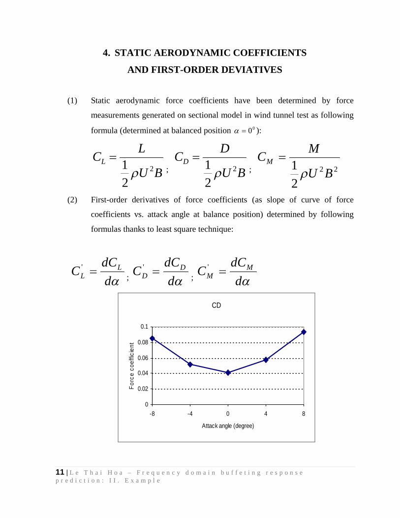
4. STATIC AERODYNAMIC COEFFICIENTS
AND FIRST-ORDER DEVIATIVES
(1) Static aerodynamic force coefficients have been determined by force
measurements generated on sectional model in wind tunnel test as following
formula (determined at balanced position 00 ):
BU
LCL2
21
; BU
DCD2
21
; 22
21 BU
MCM
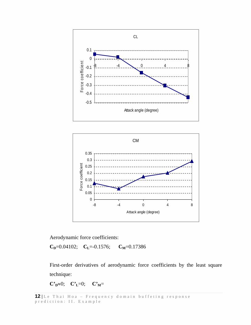
(2) First-order derivatives of force coefficients (as slope of curve of force
coefficients vs. attack angle at balance position) determined by following
formulas thanks to least square technique:
ddC
C LL '
; ddC
C DD '
; ddC
C MM '
CD
0
0.02
0.04
0.06
0.08
0.1
-8 -4 0 4 8
Attack angle (degree)
Forc
e co
effic
ient
12 | L e T h a i H o a – F r e q u e n c y d o m a i n b u f f e t i n g r e s p o n s e p r e d i c t i o n : I I . E x a m p l e
CL
-0.5
-0.4
-0.3
-0.2
-0.1
0
0.1
-8 -4 0 4 8
Attack angle (degree)
Forc
e co
effic
ient
CM
0
0.05
0.1
0.15
0.2
0.25
0.3
0.35
-8 -4 0 4 8
Attack angle (degree)
Forc
e co
effic
ient
Aerodynamic force coefficients:
CD=0.04102; CL=-0.1576; CM=0.17386
First-order derivatives of aerodynamic force coefficients by the least square
technique:
C’D0; C’L=0; C’M=

13 | L e T h a i H o a – F r e q u e n c y d o m a i n b u f f e t i n g r e s p o n s e p r e d i c t i o n : I I . E x a m p l e
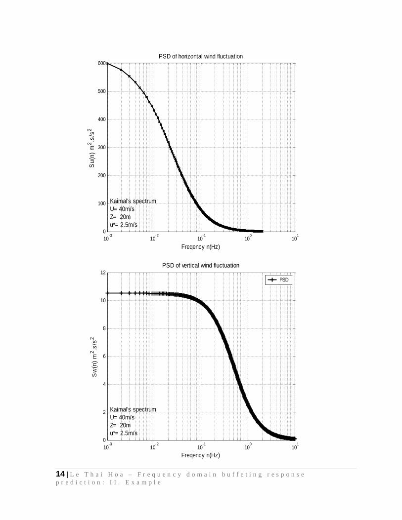
5. POWER SPECTRAL DENSITY (PSD) OF FLUCTUATIONS
(1) Deck elevation: Z=20m; static wind velocity U=20m/s
(1) One-sided power spectral density (PSD) functions determined by empirical
formulas in which PSD of horizontal wind fluctuation determined by
Kaimail’s spectrum, whereas PSD of vertical wind fluctuation computed by
Buches and Panofsky’s spectrum
3/5
2*
501200)(
fnfunSu
(Kaimal’s spectrum)
f: Non-dimensional Monin coordinates, Unzf
n: Frequency (Hz)
U,z: Mean velocity (m/s) and structural altitude z (m), respectively
u*: Friction or shear velocity (m/s), )/ln(* zozkUu
k, z0: Scale factor and roughness length (m)
k=0.4 and z0=2.5 : Simui&Scanlan (1976)
3/5
2*
10136.3)(
fnufnSw
(Panofsky’s spectrum)
14 | L e T h a i H o a – F r e q u e n c y d o m a i n b u f f e t i n g r e s p o n s e p r e d i c t i o n : I I . E x a m p l e
10-3
10-2
10-1
100
101
0
100
200
300
400
500
600PSD of horizontal wind fluctuation
Freqency n(Hz)
Su(
n) m
2 .s/s
2
Kaimal's spectrumU= 40m/sZ= 20mu*= 2.5m/s
10-3
10-2
10-1
100
101
0
2
4
6
8
10
12PSD of vertical wind fluctuation
Freqency n(Hz)
Sw
(n) m
2 .s/s
2
PSD
Kaimal's spectrumU= 40m/sZ= 20mu*= 2.5m/s

15 | L e T h a i H o a – F r e q u e n c y d o m a i n b u f f e t i n g r e s p o n s e p r e d i c t i o n : I I . E x a m p l e
6. AERODYNAMIC ADMITTANCE (1) Some empirical formulas can be applied for aerodynamic admittance such as
Sears’s function(1935), Liepmann’s function(1952), Davenport’s function
(1963) and Irwin’s function (1977).
(2) Liepmann’s function is often used in analytical buffeting response prediction
UBn
ni
i 22
21
1)(
(Liepmann’s function)
10-2 10-1 100 1010
0.1
0.2
0.3
0.4
0.5
0.6
0.7
0.8
0.9
Frequency Log(n)
Aer
odyn
amic
adm
ittan
ce
(Inputs: B=15m, U=20m/s)
16 | L e T h a i H o a – F r e q u e n c y d o m a i n b u f f e t i n g r e s p o n s e p r e d i c t i o n : I I . E x a m p l e
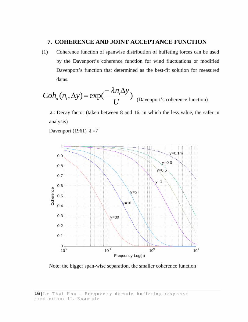
7. COHERENCE AND JOINT ACCEPTANCE FUNCTION (1) Coherence function of spanwise distribution of buffeting forces can be used
by the Davenport’s coherence function for wind fluctuations or modified
Davenport’s function that determined as the best-fit solution for measured
datas.
)exp(),(U
ynynCoh iiu
(Davenport’s coherence function)
: Decay factor (taken between 8 and 16, in which the less value, the safer in
analysis)
Davenport (1961) =7
10-2 10-1 100 1010
0.1
0.2
0.3
0.4
0.5
0.6
0.7
0.8
0.9
1
Frequency Log(n)
Coh
eren
ce
y=0.1m
y=0.3
y=0.5
y=1
y=5
y=10
y=30
Note: the bigger span-wise separation, the smaller coherence function

17 | L e T h a i H o a – F r e q u e n c y d o m a i n b u f f e t i n g r e s p o n s e p r e d i c t i o n : I I . E x a m p l e
(2) In this numerical example, spanwise separation holds 5m that is distance
between every two deck nodes.
8. STRUCTRURAL AND AERODYNAMIC DAMPINGS
8.1. Strucrural damping ratio (1) Two type of dampings can be used in dynamic analyses
Damping ratio: ii
isi km
c2
Logarithmic decrement (logdec): )()(log1
tynTty
nTsi
.100%
Relationship: 2
sisi
(2) System damping ratio in wind-induced vibrations combines between
structural damping and aerodynamic damping that are associated with any
mode in the mode-based analysis
aisii
(3) Structural damping can be estimated by model-scaled and full-scaled
free/forced/ambiemt vibration tests
(4) It is generally agreed to assume that structural damping ratio is taken 0.03
for all modes, corresponding to logarithmic decrement 0.5% (Actually,
structrural damping increases with the order of high-frequency modes)
03.0si
8.2. Aerodynamic damping ratio

18 | L e T h a i H o a – F r e q u e n c y d o m a i n b u f f e t i n g r e s p o n s e p r e d i c t i o n : I I . E x a m p l e
(1) Aerodynamic damping ratio can be determined by physical measurement of
aerodynamic damping force on either 2D sectional model or 3D elastic model
(2) Aerodynamic damping ratio can be estimated for all modes in three
displacement components by either of:
From quasi-steady aerodynamic forces: (The same for all modes)
mB
BfUC
Z
LaZ
2'
8
(Vertical response prediction)
mB
BfUC
X
DaX
2
4
(Horizontal response prediction)
IB
BfUCM
a
4'
8
(Rotational response prediction)
From flutter derivatives: (Different from each modes)
mBfHf jjaZ 2
)()(2
*1
mBfPf jjaX 2
)()(2
*1
IBfAf jja 2
)()(4
*2
(3)System damping ratios of 5 fundamental modes have been computed as follows:
Modes s,i a,i i
Mode 1 0.005 0.00121 0.00621 Mode 2 0.005 0.000912 0.005912
19 | L e T h a i H o a – F r e q u e n c y d o m a i n b u f f e t i n g r e s p o n s e p r e d i c t i o n : I I . E x a m p l e
Mode 3 0.005 0.0001 0.0051 Mode 4 0.005 0.0000716 0.005072 Mode 5 0.005 0.0000571 0.005057
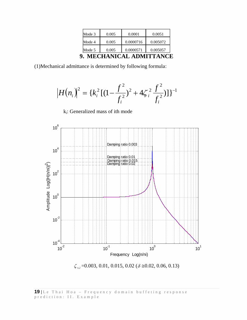
9. MECHANICAL ADMITTANCE (1)Mechanical admittance is determined by following formula:
12
222
2
222 )]}4)1[({
ii
iii f
fffknH
ki: Generalized mass of ith mode
10-2 10-1 100 10110-4
10-2
100
102
104
106
Frequency Log(n/ni)
Am
plitu
de L
og(|H
(n/n
i)|2 )
Damping ratio 0.003
Damping ratio 0.01 Damping ratio 0.015 Damping ratio 0.02
is , =0.003, 0.01, 0.015, 0.02 ( 0.02, 0.06, 0.13)

20 | L e T h a i H o a – F r e q u e n c y d o m a i n b u f f e t i n g r e s p o n s e p r e d i c t i o n : I I . E x a m p l e
Noting that with different damping ratio, the background response component
stays the constant, whereas the resonance response differs at peak values that
depends on damping value (the smaller damping ratio, the bigger mechanical
admittance)
10. RESULTS AND REMARKS
0
0.1
0.2
0.3
0.4
0.5
0.6
0.7
10 20 30 40 50 60
Mean wind velocity
RM
S o
f Ver
tical
dis
p. (m
)
RMS response of vertical displacement at midspan node
Mode 1
Mode 2 Mode 5

21 | L e T h a i H o a – F r e q u e n c y d o m a i n b u f f e t i n g r e s p o n s e p r e d i c t i o n : I I . E x a m p l e
00.10.20.30.40.50.60.70.8
10 20 30 40 50 60
Mean wind velocity U(m/s)
Res
pons
e (D
egre
e)
RMS response of rotational displacement at midspan node
RMS of Total response (Degree)
0
0.2
0.4
0.6
0.8
10 20 30 40 50 60
Mean wind velocity U(m/s)
RMS of total response of rotational displacement at midspan node
(SRSS response combination)
Mode 3
Mode 4
22 | L e T h a i H o a – F r e q u e n c y d o m a i n b u f f e t i n g r e s p o n s e p r e d i c t i o n : I I . E x a m p l e
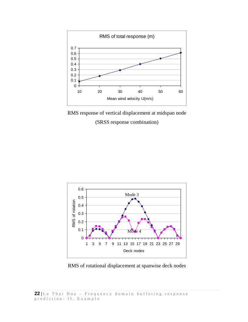
RMS of total response (m)
00.10.20.30.40.50.60.7
10 20 30 40 50 60
Mean wind velocity U(m/s)
RMS response of vertical displacement at midspan node
(SRSS response combination)
0
0.1
0.2
0.3
0.4
0.5
0.6
1 3 5 7 9 11 13 15 17 19 21 23 25 27 29
Deck nodes
RM
S o
f rot
atio
n
RMS of rotational displacement at spanwise deck nodes
Mode 3
Mode 4
23 | L e T h a i H o a – F r e q u e n c y d o m a i n b u f f e t i n g r e s p o n s e p r e d i c t i o n : I I . E x a m p l e
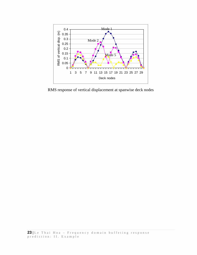
00.050.1
0.150.2
0.250.3
0.350.4
1 3 5 7 9 11 13 15 17 19 21 23 25 27 29
Deck nodes
RM
S o
f ver
tical
dis
p. (m
)
RMS response of vertical displacement at spanwise deck nodes
Mode 1
Mode 2
Mode 5