Frequency Domain Analysis In

7/30/2019 Frequency Domain Analysis In

http://slidepdf.com/reader/full/frequency-domain-analysis-in 1/8

paper 6601

Frequency Domain Analysis in Rotor/Stator Contact Problems

Gotz von Groll and David J Ewins

Imperial College of Science Technology & Medicine, Mech. Eng. Dep.London SW7 2BX, UK

[email protected]

Abstract

There are a variety of abnormal running conditions in rotating machinery which lead torotor/stator dynamics interactions which, in turn, can cause a rich mixture of effects asso-ciated with rub-related phenomena. These effects manifest themselves in the occurrence of multiple solutions for steady-state vibration response scenarios, including amplitude jumpsduring rotor acceleration, and vibration responses at different/multiple frequencies of exci-tation forces such as unbalance. This paper describes a numerical algorithm based on theharmonic balance method to calculate the periodic response of a non-linear system under pe-riodic excitation. The algorithm also calculates the stability of the periodic solutions found,

marks turning and bifurcation points, and follows a solution branch over varying systemparameters via arc-length continuation.

1 INTRODUCTION

The motivation for this study comes from rotor/stator contact induced vibration prob-lems in turbo-machinery. They can include: rotors touching seals, rotor touching retain-er bearings when main active magnetic bearings fail, inter-shaft contact in multiple spoolengines, rotor blades contacting the stator, increased bearing clearance through wear oroutright bearing failure. In many of these scenarios the rotor continues to rotate and so, de-pending on the problem, it is often the steady-state response to the out-of-balance excitation

forces which is of concern, rather than a particular transient event.Both the harmonic balance method (HBM) and continuation schemes are well-known

numerical tools to study nonlinear dynamics problems. However, they seem to be usedrarely in conjunction with each other in engineering applications, as continuation appearsmore frequently with time-domain methods, such as shooting or boundary value problemsolvers, whereas the HBM is essentially a frequency-domain method. Rotor dynamics ex-amples using time-domain methods with continuation are: Sundararajan and Noah (1997)for squeeze-film-damper and journal bearing analysis and Petrov (1996) for shroud/bladefriction. Harmonic balance is not only convenient for purposes of linearisation of systemswith small non-linearities (Geradin and Kill, 1988), but can can also be applied to large

non-linearities (Choi and Noah, 1988). Kim et al. (1991) analysed the behaviour of rotors



paper 6602

with bearing housing clearances using the HBM at discrete speeds but without continuation.

As with most numerical techniques, calculating the Jacobian (most probably by numericalfinite difference estimation) is part of solving the equations set up by the harmonic balancemethod (Gasch and Knothe, 1989). It will be shown that the availability of the Jacobianmeans that the HBM lends itself nicely to studies of the stability of a solution without havingto go back into the time domain (Floquet analysis). Such an algorithm for a non-linear systemis based on the approach for linear time-variant systems. Naturally, the algorithm describedhere is also applicable to other common non-linear elements in structural dynamics.

2 HARMONIC BALANCE FORMULATION

Given the computing resources, the HBM is easily applicable to problems with a large

number of degrees-of-freedom (DOFs). Typically, such a problem consists of finite elemen-t models of large parts of the structure or substructures where a linear representation isadequate, and some ‘problematic’ DOFs for special areas, e.g. where friction, impacts, orother interaction occurs. Usually, the linear DOFs outnumber the nonlinear ones by a largeratio. The example that will be used later on deals with the dynamics when rotor and statorcome into contact. The rotor and stator are modelled as linear structures, and there will besome linear external forces like gravity and out-of-balance. The contact region supplies thenonlinear forcing at a few degrees of freedom on both rotor and stator.

For simplicity, the complete system is split into its linear part, represented by the usualmass, stiffness, damping matrices, with some linear external force vector, f u (e.g. un-

balance), and its nonlinear part, which is represented here as a single force vectorf

c

combining all nonlinear effects (contact between rotor and stator):

[M ]

r

+ [C ]

r

+ [K ]

r

=

f u(t)

+

f c(r)

(1)

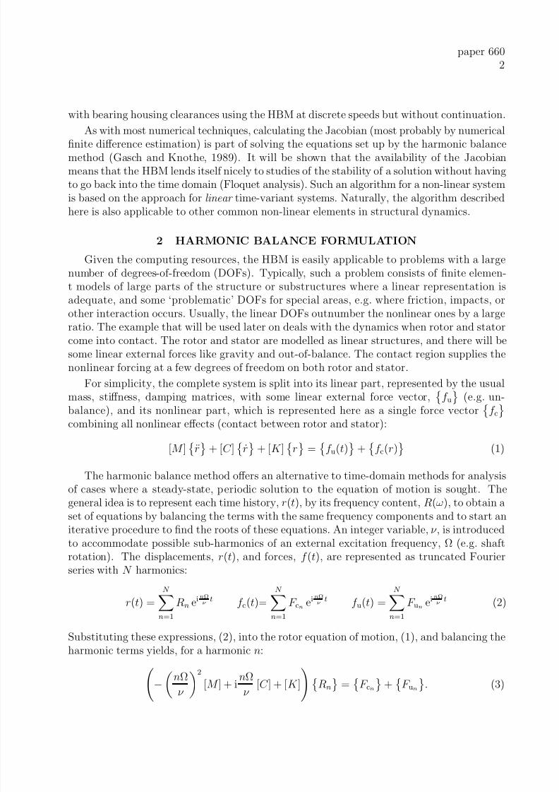
The harmonic balance method offers an alternative to time-domain methods for analysisof cases where a steady-state, periodic solution to the equation of motion is sought. Thegeneral idea is to represent each time history, r(t), by its frequency content, R(ω), to obtain aset of equations by balancing the terms with the same frequency components and to start aniterative procedure to find the roots of these equations. An integer variable, ν , is introducedto accommodate possible sub-harmonics of an external excitation frequency, Ω (e.g. shaft

rotation). The displacements, r(t), and forces, f (t), are represented as truncated Fourierseries with N harmonics:

r(t) =N n=1

Rn einΩ

νt f c(t)=

N n=1

F cn einΩ

νt f u(t) =

N n=1

F un einΩ

νt (2)

Substituting these expressions, (2), into the rotor equation of motion, (1), and balancing theharmonic terms yields, for a harmonic n:

−nΩ

ν 2

[M ] + inΩ

ν

[C ] + [K ]Rn = F cn + F un. (3)



paper 6603

Bringing all N harmonics into one equation can be symbolised as

K

R−

F c−

F u

= 0 (4)

and

R

and

F

are the vectors of Fourier coefficients of displacements and forces, re-spectively. As the Fourier coefficients, F cn, of the non-linear forces, f c, are functions of thedisplacements (and thus their respective Fourier coefficients),

F cn = F cn(R0(ω0), R1(ω1), . . . , RN (ωN )), (5)

equation (4) is non-linear and must be solved iteratively. This iteration process (Kim et al.,1991) can be sketched as:

R(ω)(k)FT−1−−−→ r(t)(k) → f c(t)(k+1)

FT−−−→ F c(ω)(k+1) → R(ω)(k+1)

Finite element models of rotor/stator structures can contain quite a large number of degrees-of-freedom. Setting up equation (4) then leads to a much bigger problem with 2N + 1 timesmore unknowns (real and imaginary components for N harmonics and a DC component).

Reduction The harmonic balance method offers an elegant means of reducing the problemorder, so that only the non-linear DOFs need to be kept (Kim et al., 1991). Clearly beingable to keep only the non-linear DOFs vastly increases the speed in cases of linear structureswhich have a few additional non-linear elements, as is typical for many classes of problems.

The equation (3) is re-ordered for every harmonic, n (the subscripts n are omitted in thissection for clarity):

K mm K ms

K sm K ss

Rm

Rs

=

F c0

+

F umF us

(6)

where subscripts m and s stand for non-linear (master) and linear (slave) degrees-of-freedom,respectively. It follows that

ˆ

K = K mm− K ms K ss−1

K sm (7)

ˆ

F u

=

F um−

K ms

K ss

−1

F us

(8)

and

ˆK

Rm

−

F c− ˆ

F u

= 0 (9)

In contrast to the widely-used Guyan reduction, equation (9) is an exact reduction of theoriginal problem as long as the prerequisites for applying the harmonic balance method aremet and the number of harmonics included in the decomposition is sufficient.



paper 6604

Continuation Usually, the system behaviour is of interest over a range of values for atleast one parameter (e.g. speed of shaft rotation), so that the solution has to be calculated

at different parameter values consecutively. Any continuation scheme is just as applicable inthe frequency domain as it is in the time-domain. The task of finding a periodic solution forequation (1) can be transformed into an equivalent root-finding problem in either time orfrequency domain, for example by means of finite difference, shooting, HBM. An arc-lengthcontinuation scheme may then be employed to move along the arc-length α of a solutionbranch of the root-finding problem, facilitating the passing of turning points (overhung partof the solution branches). Continuation schemes are standard tools and the reader is referredto Seydel (1994); Nayfeh and Balachandran (1995) for a detailed treatment.

3 STABILITY

When HBM with arc-length continuation is employed, there is nothing in the algorithmper se that can warn the user that a particular solution branch followed has stepped over aturning or bifurcation point and the solution has switched stability, from stable to unstable,or vice versa. For example, there might only be a little change in the conditioning of the Jacobian of the system before and after such a change, nor is there a change in theconvergence behaviour of the algorithm. This is a practical problem (not a theoretical one,as the Jacobian F y is indeed singular exactly on a turning or bifurcation point) as changein conditioning of the Jacobian could occur far more rapidly than the step-length is ableto resolve. However, at little cost, stability can be analysed with a modification of analgorithm employed for linear time-variant systems. The algorithm is called Hill’s method

and transforms a linear time-variant system into an eigenvalue problem of a linear time-invariant system (Gasch and Knothe, 1989). In order to use the same approach for non-linearsystems, the stability analysis is carried out by investigating the effect of a perturbationaround a periodic solution r(t). Let the perturbation be described as p(t), where p(t)consists of a decay term eλt and a periodic term s(t) (Genta, 1999):

p(t) = eλt s(t) s(t)=N

n=−N

S n einΩ

νt (10)

Assigning r(t) = r(t) + p(t) and by substituting the Fourier representations of r(t), s(t) ,the harmonic components can be balanced in an analogue manner to equation (4):

K

R

+

λ2

M

+ λ

C

+

K

S

eλt

=

F u

+

F c

R + S eλt (11)

where

M

,

C

are constructed in a similar manner to

K

in equation (4) and

R(ω)

,S (ω)

are the vectors of Fourier coefficients for r(t), s(t), respectively.

In what follows, an attempt is being made to find a cost-effective linearisation for theterm

F c

R + S eλt

so that equation (11) can be developed further. Consider a variantof equation (4):

F c

=

K

R−

F u−

E (R)

(12)



paper 6605

where

E (R)

is the error in the balancing terms. Developing this as a Taylor series around

a known solution of equation (4), R, one obtainsF c(R)

=

K

R−

F u− [E (R)]

R−

R

+ higher order terms (13)

with the abbreviation [E ] =∂E ∂R

. Substituting equation (13) into (11) and neglecting terms

of higher order, equation (11) simplifies to the following eigenvalue problem:λ2

M

+ λ

C

+ [E (R)]

S

= 0. (14)

It is important to note that the term [E (R)] is already available as a by-product of thequasi-newton solution technique, most probably as a numerical approximation, as it is theJacobian of the objective function defined by equation (4).

Solving for the eigenvalues of equation (14), one obtains a set of λi with real and imaginaryparts, where a negative real part indicates stability of the solution, as the perturbation p(t)decays with time, and a positive real part indicates instability. So by solving this eigenvalueproblem at the end of the overall iteration procedure, and simply checking if any λi possessesa real part > 0, one can easily determine whether a periodic solution r(t) is unstable. Thisalso helps with finding possible bifurcation points. A change in stability of a solution branchis a sufficient indicator that a turning or bifurcation point has been passed, and the algorithmcould be directed to determine the cross-over point within this interval of change more closely.Should this be of interest and the cross-over point found, the rank of F y and

F y F Ω

at the

cross-over determines whether the point in question is a turning or bifurcation point (Seydel,

1994). If indeed it is a bifurcation point a further solution branch may be followed.

4 NUMERICAL EXAMPLE

Although the algorithm described above is easily scalable to systems with a large numberof degrees of freedom, a simple modified Jeffcott rotor (Figure 1) is used here for clarity.The equations of motion for a Jeffcott rotor interacting with a linear stator structure are:

mrrr + crrr + krrr = −f c + Ω2mrm eiΩt (15)

msrs + csrs + ksrs = f c (16)

y

x z

Figure 1: A Jeffcott rotor with stator



paper 6606

0.5 1 1.5 2

1

2

3

4

5

6

7

Ω

| r |

rotor

stator

gap

5 5.5 6 6.5 7 7.50.8

0.85

0.9

0.95

1

1.05

1.1

1.15

1.2

Ω

| r | rotor without stator contact

rotor with stator contact

Figure 2: response magnitude at constant speed. solution: + stable, o unstable

where rr, rs are the rotor and stator displacements in the complex plane and f c is the contactforce between rotor and stator, f c = kcδ where δ is the depth of the contact described belowin (17) and kc the local (in this case linear) contact stiffness (for more realistic simulationsone would have to choose a nonlinear contact force, see Fumagalli and Schweitzer (1996)).For the purpose of numerical simulation, a small contact penetration δ of the rotor andstator rings is allowed. The contact stiffness kc in this penetration region is being set to avalue orders of magnitude higher than the rotor shaft or stator suspension stiffness, so thatthe penetration depth is orders of magnitude lower than rotor and stator deflections. The

contact depth is defined as

δ (t) =

rr + r eiΩt−rs − s − h eiψ if |rr + r eiΩt−rs − s| > h,

0 otherwise(17)

where rr, rs are rotor and stator displacements, h is the gap size, r a possible offset of therotor disc and s a stator offset. These entities are depicted in Figure 1.

For the special case of full annular rub with r, s = 0 and isotropic rotor supports, theequations of motion become quasi-static for pure forward or backward whirl. At a givenspeed, the steady-state conditions of rotor whirl are such that the radial deflection of therotor is constant. The only frequency component in the unbalance response spectrum isthus the engine-order speed, Ω. This simple case is used here to illustrate the stability andcontinuation study. In Figure 2 the magnitudes of the rotor and stator responses rr, rs areplotted versus the rotor speed of rotation Ω. One can see that at speeds Ω < 0.9 the rotorunbalance response is too low to overcome the clearance (h = 3, dashed line) and rotor andstator are not in contact (stator response zero). At speeds 0.9 < Ω < 1.4 rotor and statorare in contact (non-zero stator response), albeit the overhung part of the curve represents anunstable solution. At speeds Ω > 1.4, well past the natural frequency of the rotor, which hasbeen normalised to ωr = 1, the super-critically running rotor loses contact with the stator.

Figure 2b shows a second solution branch at Ω > 6, which is not seen in the 1 DOFDuffing type oscillators that display only the overhung behaviour in Figure 2. It must benoted that by following the branch previously discussed, the one that lost contact with the



paper 6607

5

10

15

20

0

2

4

6−100

−50

0

50

[Hz][EO]

[ d B ]

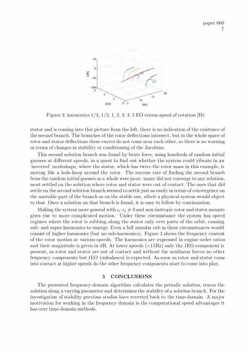
Figure 3: harmonics 1/3, 1/2, 1, 2, 3, 4, 5 EO versus speed of rotation [Hz]

stator and is coming into this picture from the left, there is no indication of the existence of the second branch. The branches of the rotor deflections intersect, but in the whole space of rotor and stator deflections these curves do not come near each other, so there is no warningin terms of changes in stability or conditioning of the Jacobian.

This second solution branch was found by brute force, using hundreds of random initialguesses at different speeds, in a quest to find out whether the system could vibrate in an‘inverted’ modeshape, where the stator, which has twice the rotor mass in this example, ismoving like a hola-hoop around the rotor. The success rate of finding the second branchfrom the random initial guesses as a whole were poor: many did not converge to any solution,

most settled on the solution where rotor and stator were out of contact. The ones that didsettle on the second solution branch seemed to settle just as easily in terms of convergence onthe unstable part of the branch as on the stable one, albeit a physical system would objectto that. Once a solution on that branch is found, it is easy to follow by continuation.

Making the system more general with r, s = 0 and non-isotropic rotor and stator mountsgives rise to more complicated motion. Under these circumstance the system has speedregimes where the rotor is rubbing along the stator only over parts of the orbit, causingsub- and super-harmonics to emerge. Even a full annular rub in these circumstances wouldconsist of higher harmonics (but no sub-harmonics). Figure 3 shows the frequency contentof the rotor motion at various speeds. The harmonics are expressed in engine order ratios

and their magnitude is given in dB. At lower speeds (<15Hz) only the 1EO component ispresent, as rotor and stator are out of contact and without the nonlinear forces no otherfrequency components but 1EO (unbalance) is expected. As soon as rotor and stator comeinto contact at higher speeds do the other frequency components start to come into play.

5 CONCLUSIONS

The presented frequency-domain algorithm calculates the periodic solution, traces thesolution along a varying parameter and determines the stability of a solution branch. For theinvestigation of stability previous studies have reverted back to the time-domain. A majormotivation for working in the frequency domain is the computational speed advantages it

has over time-domain methods.



paper 6608

The solution process of the HBM method itself is less expensive than time-domain meth-ods, and the reduction to the non-linear degrees-of-freedom offers vast savings in large finite

element models with only a few non-linear components. It was found that in the given nu-merical example the harmonic balance method was over 100 times faster than time-domainshooting and boundary-value-problem solving.

HBM also functioned properly in many instances where the time integration routines haddifficulties. The source of these difficulties lies in the contact problem. As both rotor andstator have non-negligible mass (and thus dynamics in their own right), the penalty stiffnesskc determines the violence of the rotor/stator impacts and thus tests the robustness andinfluences the speed of convergence of any chosen method.

A more sophisticated contact model can alleviate this problem to a large extent. However,there are situations where the harmonic balance method does not find a solution. This is

usually an indication that not enough or not the right harmonic components are includedin the setup. This can probably be circumvented by choosing a hybrid approach of aninitial setup in time-domain and continuation in frequency-domain. This approach will beinvestigated in future work.

Acknowledgements

The authors are grateful to Rolls-Royce plc. for providing financial and technical supportfor this project and for giving permission to publish this work.

References

Choi, Y.-S. and Noah, S. T. (1988). Forced periodic vibraton of unsymmetric piecewise-linearsystems. Journal of Sound and Vibration , 121(1):117–126.

Fumagalli, M. and Schweitzer, G. (1996). Measurements on a rotor contacting its housing.In Sixth International Conference on Vibrations in Rotating Machinery , pages 779–788,Oxford. Institution of Mechanical Engineers.

Gasch, R. and Knothe, K. (1989). Strukturdynamik II . Springer.

Genta, G. (1999). Vibration of Structures and Machines . Springer, third edition.

Geradin, M. and Kill, N. (1988). Non-linear dynamic analysis of flexible rotors. In Fourth

International Conference on Vibrations in Rotating Machinery , pages 627–634. Institutionof Mechanical Engineers.

Kim, Y. B., Noah, S. T., and Choi, Y.-S. (1991). Periodic response of multi disk rotors withbearing clearances. Journal of Sound and Vibration , 144(3):381–395.

Nayfeh, A. and Balachandran, B. (1995). Applied Nonlinear Dynamics . John Wiley & Sons.

Petrov, E. (1996). Analysis of periodic regimes of forced, essentially nonlinear vibrationsof systems of turbine blades. In Numerical Methods in Engineering ’96 , pages 924–930,Paris. ECCOMAS Conference, John Wiley & Sons.

Seydel, R. (1994). Practical Bifurcation and Stability Analysis . Springer.

Sundararajan, P. and Noah, S. T. (1997). Dynamics of forced nonlinear systems usingshooting / arc-length continuation method — application to rotor systems. Transactions

of the ASME, Journal of Vibration and Acoustics , 119:9–20.

Frequency Domain Analysis In

Documents

Transcript of Frequency Domain Analysis In