Free Vibration of Single-Degree- of- Freedom Systemsdrahmednagib.com/onewebmedia/Vibration...
22
Dr. Bassuny El-Souhily Chapter II Mechanical Vibrations 41 CHAPTER 3 Free Vibration of Single-Degree- of- Freedom Systems Systems are said to undergo free vibration when they oscillate about their static equilibrium position when displaced from those positions and then released. The frequencies at which they vibrate, known as natural frequencies, depend primarily upon the mass and elasticity (stiffness) of the systems. Free vibration of an undamped system: Equation of motion a- Using Newton’s second law of motion: 1- Select a suitable coordinate to describe the position of the mass or the rigid body in the system, (Linear coordinate for linear motion-Angular coordinate for angular motion), 2- Determine the static equilibrium configuration of the system and measure the displacement from it, 3- Draw the free-body diagram of the mass or rigid body, indicate all the active and reactive forces acting on the system, 4- Apply Newton’s second law of motion to the mass or rigid body shown by the free-body Diagram. ”The rate of change of momentum of a mass is equal to the forces acting on it” Example 1: Mass-spring system i- . m ≡ mass in Kg k ≡ spring stiffness N/m (weightless spring) "# = −'# "# + '# = 0
Transcript of Free Vibration of Single-Degree- of- Freedom Systemsdrahmednagib.com/onewebmedia/Vibration...
Dr.$Bassuny$El-Souhily$Chapter$II$Mechanical$Vibrations$$
41$$
CHAPTER 3 Free Vibration of Single-Degree- of- Freedom Systems Systems are said to undergo free vibration when they oscillate about their static equilibrium position when displaced from those positions and then released. The frequencies at which they vibrate, known as natural frequencies, depend primarily upon the mass and elasticity (stiffness) of the systems.
Free vibration of an undamped system:
Equation of motion
a-!Using Newton’s second law of motion: 1-! Select a suitable coordinate to describe the position of the mass or the rigid
body in the system, (Linear coordinate for linear motion-Angular coordinate for angular motion),
2-!Determine the static equilibrium configuration of the system and measure the displacement from it,
3-!Draw the free-body diagram of the mass or rigid body, indicate all the active and reactive forces acting on the system,
4-! Apply Newton’s second law of motion to the mass or rigid body shown by the free-body Diagram. ”The rate of change of momentum of a mass is equal to the forces acting on it”
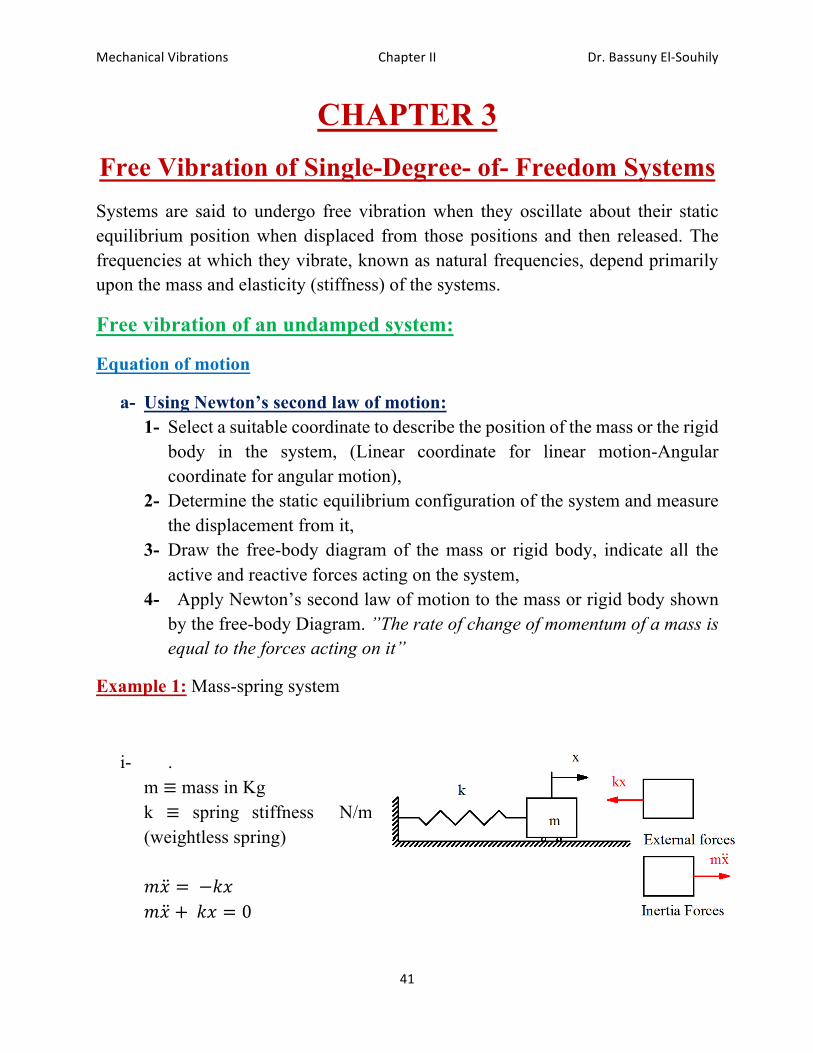
Example 1: Mass-spring system
i-! . m ≡ mass in Kg k ≡ spring stiffness N/m (weightless spring) "# = %−'# "# + %'# = 0
Dr.$Bassuny$El-Souhily$Chapter$II$Mechanical$Vibrations$$
42$$
# +'"# = 0%%
# +%*+,%# = 0%%-. /.0%%
*+ = %'"%%1234%%
*+ ≡ natural frequency (circular) 5 = %67
,8( cps) Hz
9:1;<3%= =2?*+
=15%%%4:A.
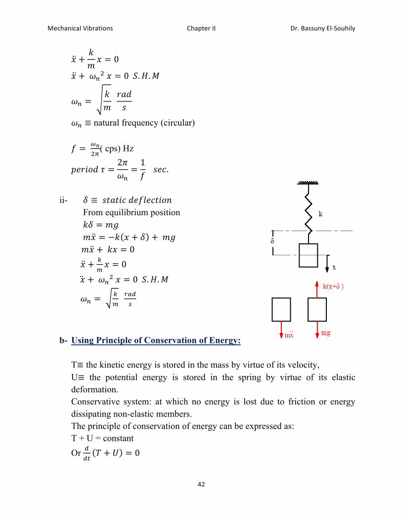
ii-! B ≡ %4C2C;A%3:5D:AC;<E
From equilibrium position 'B = "F%%% "# = −' # + B + %"F
%%%%%"# + %'# = 0 # + G
H# = 0%%
%# +%*+,%# = 0%%-. /.0%%
*+ = %G
H%%IJK
L%%
b-!Using Principle of Conservation of Energy: T≡ the kinetic energy is stored in the mass by virtue of its velocity, U≡ the potential energy is stored in the spring by virtue of its elastic deformation. Conservative system: at which no energy is lost due to friction or energy dissipating non-elastic members. The principle of conservation of energy can be expressed as: T + U = constant Or K
KMN + O = 0
Dr.$Bassuny$El-Souhily$Chapter$II$Mechanical$Vibrations$$
43$$
In example 1-i
N = %12%"#,%%
O =12'#,%%
33C
12%"#, +
12'#, = 0
%%%%%"# + %'# = 0 1-ii
N = %12%"#,%%
O =12'(# + B), − "F%#%
33C
12%"#, +
12' # + B , − "F%# = 0%
"## + ' # + B # − "F# = 0 'B = "F%%%
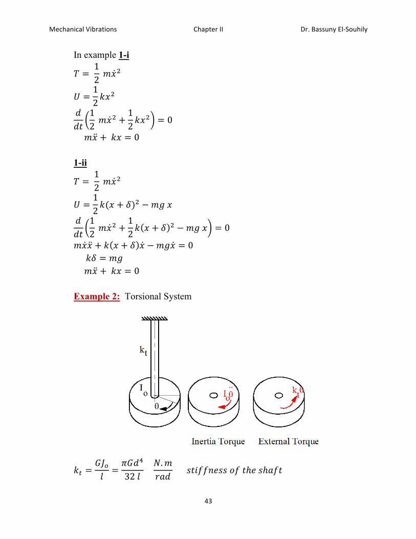
%%%%%"# + %'# = 0 Example 2: Torsional System
'M =RSTD=?R3U
32%D%%%%W."123
%%%%%%4C;55E:44%<5%Cℎ:%4ℎ25C%%
Dr.$Bassuny$El-Souhily$Chapter$II$Mechanical$Vibrations$$
44$$
YTZ = −'MZ% YT = "244%"<":EC%<5%;E:1C;2%[F.",
*+ = %G\]^%%IJK
L%%
Energy method
N = %12%Y_Z,%%
O =12'MZ,%%
33C
%12%Y_Z, %+
12'MZ,% = 0
YTZ = −'MZ%
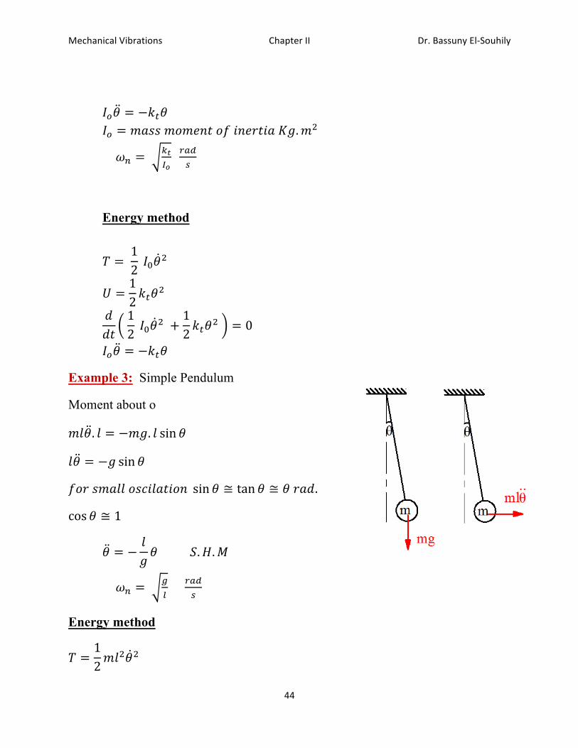
Example 3: Simple Pendulum
Moment about o
"DZ. D = −"F. D sin Z%%
DZ = −F sin Z
5<1%4"2DD%<4A;D2C;<E% sin Z ≅ tan Z ≅ Z%123.%%
cos Z ≅ 1
Z = −DFZ%%%%%%%%%%%-. /.0
*+ = %h
i%%%%%IJK
L%%
Energy method
N =12"D,Z,%%%%
Dr.$Bassuny$El-Souhily$Chapter$II$Mechanical$Vibrations$$
45$$
O = "FD 1 − cos Z %%
33C
12"D,Z, %+ "FD 1 − cos Z = 0%
12"D,2ZZ + "FD sin Z Z = 0%%%
Z ≠ 0% sin Z ≈ Z%%%
DZ + FZ = 0%
%Z +FDZ = 0%%
*+ =FD%%%%
Solution of Equation of Motion:
The general solution of %# +%*+,%# = 0%%% Let # = :LM,%%%%%%%%%%%%%# = 4,:LM%%% 4,:LM + *+,:LM = 0%%% 4, + *+, :LM = 0%%%%:LM ≠ 0%% 4 = ±;*+%%% R:E:12D%4<DnC;<E: # = 2p:q67M + 2,:rq67M%%%% # = s cos*+C + t sin*+C %%%%= u cos *+C − v %%% # = −s*+ sin*+C + t*+ cos*+C
Initial condition:
1)! C = 0%%%%%%%# = #T%%%%%%# = 0%% s = #T,%%%%t = 0%%%% # = #T cos*+C
2)! C = 0%%%%%%%# = 0%%%%%%# = wT
Dr.$Bassuny$El-Souhily$Chapter$II$Mechanical$Vibrations$$
46$$
s = 0,%%%%t =wT*+
# =wT*+
sin*+C
3)! C = 0%%%%%%%# = #T%%%%%%# = wT
s = #T,%%%%t =wT*+
# = #T cos*+C +%wT*+
sin*+C
Rayleigh’s Energy Method: To find the natural frequencies of single degree of freedom systems NHJx = OHJx%%% # = s cos*+C %%%%%#HJx = s%%% %# = −s*+ sin*+C %%%%%#HJx = s*+%%%
NHJx =12" s*+ ,%%%%%
OHJx =12's,%%%
%12" s*+ , %=
12's,%%%%
%*+ = %'"%%%%
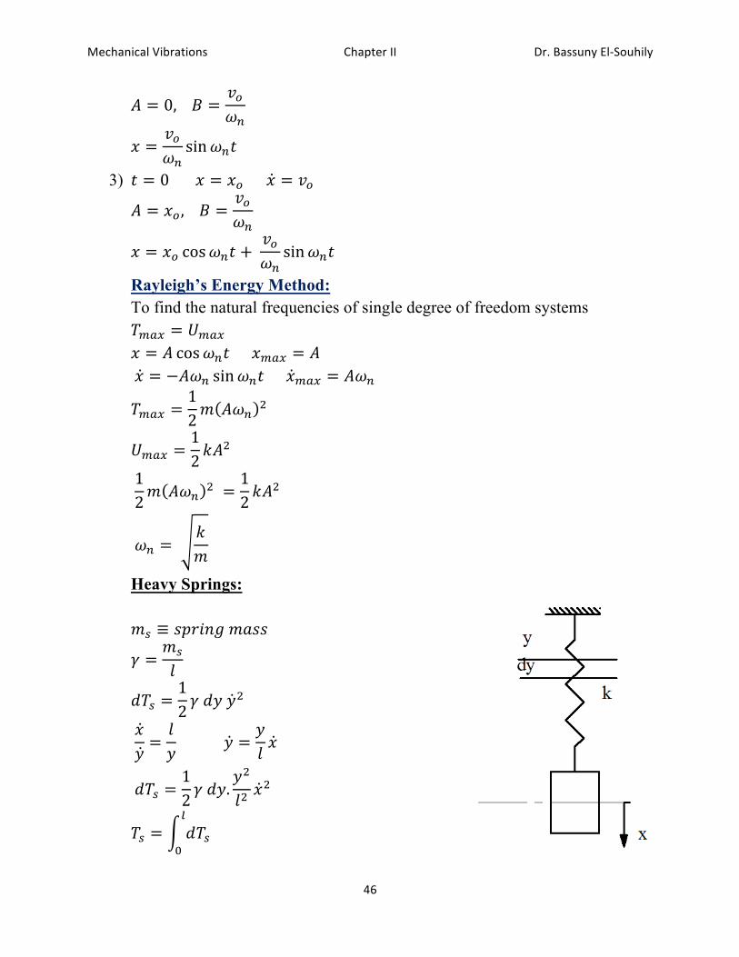
Heavy Springs: "L ≡ 491;EF%"244%%%%
y ="L
D
3NL =12y%3z%z,%%%%%%%%%%
%#z=Dz%%%%%%%%%%%%z =
zD#%%%%%
%3NL =12y%3z.
z,
D,#,%%%%
NL = 3NLi
_%%%%
Dr.$Bassuny$El-Souhily$Chapter$II$Mechanical$Vibrations$$
47$$
%%%%%=12y%D,%#, % z,3z
i
_%%%%%%
%%%%%=16yD#,%%%
%%%%%= %16"L#,%%%
N = %12%"#, +
16"L#,%%
O =12'#,%%%%%%%%%
%33C
N + O = 0
33C
12%"#, +
16"L#, +
12'#, = 0
% " +"L
3## + %'## = 0%%%%%%%%%%
% " +"L
3# + %'# = 0%%%
*+ = %'
" +"L3%%%%
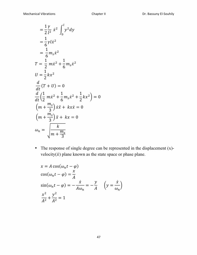
•! The response of single degree can be represented in the displacement (x)-
velocity(#) plane known as the state space or phase plane. # = s cos *+C − v %%%%%%%
cos *+C − v =#s%%%%%%%%%%
sin *+C − v = −#s*+
= −zs%%%%%% z =
#*+
%%%%
%#,
s,+z,
s,= 1
Dr.$Bassuny$El-Souhily$Chapter$II$Mechanical$Vibrations$$
48$$
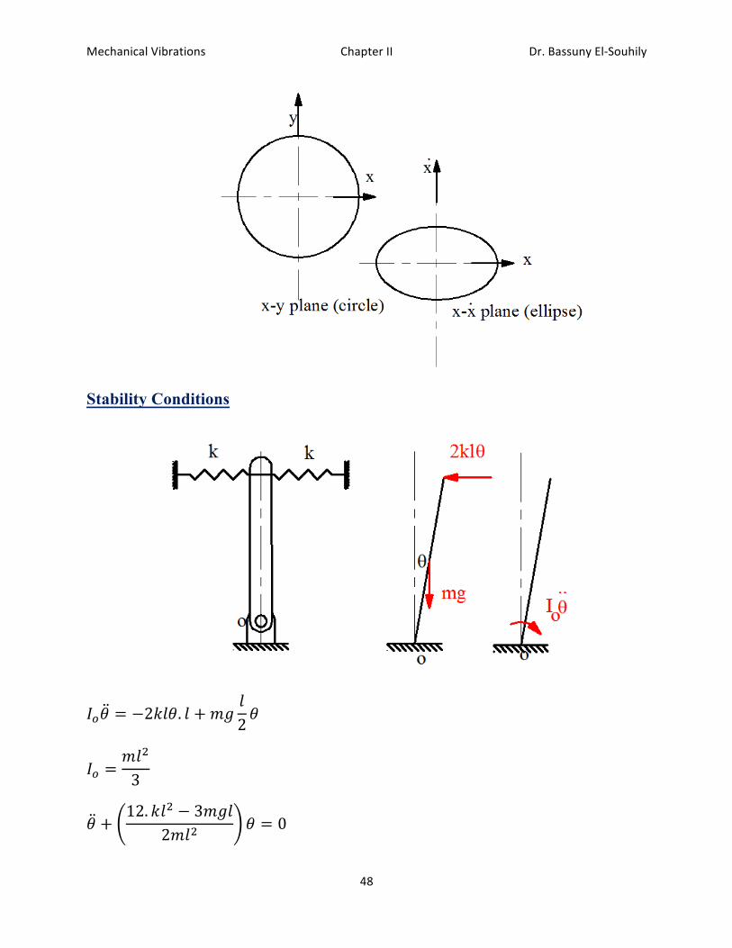
Stability Conditions
YTZ = −2'DZ. D + "FD2Z%%%%%%%%%%%%%%%%%%
YT ="D,
3%%%
Z +12. 'D, − 3"FD
2"D,Z = 0
Dr.$Bassuny$El-Souhily$Chapter$II$Mechanical$Vibrations$$
49$$
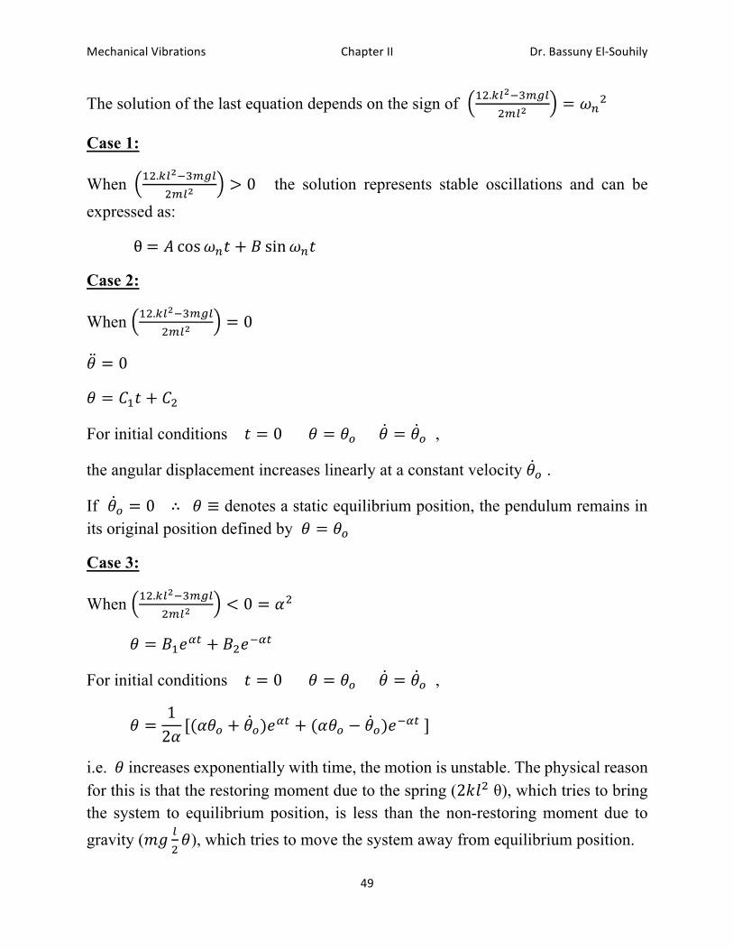
The solution of the last equation depends on the sign of p,.Gi|r}Hhi
,Hi|= *+,
Case 1:
When p,.Gi|r}Hhi
,Hi|> 0% the solution represents stable oscillations and can be
expressed as:
%θ%= s cos*+C + t sin*+C
Case 2:
When p,.Gi|r}Hhi
,Hi|= 0%
Z = 0%%%%%
Z = upC + u,
For initial conditions C = 0%%%%%%%Z = ZT%%%%%%Z = ZT ,
the angular displacement increases linearly at a constant velocity ZT .
If ZT = 0%%% ∴ %%Z ≡ denotes a static equilibrium position, the pendulum remains in its original position defined by Z = ZT%%
Case 3:
When p,.Gi|r}Hhi
,Hi|< 0 = Ç,%
Z = tp:ÉM + t,:rÉM%%%%
For initial conditions C = 0%%%%%%%Z = ZT%%%%%%Z = ZT ,
Z =12Ç
[(ÇZT + ZT):ÉM + (ÇZT − ZT):rÉM%]%%%
i.e. Z increases exponentially with time, the motion is unstable. The physical reason for this is that the restoring moment due to the spring (2'D, θ), which tries to bring the system to equilibrium position, is less than the non-restoring moment due to gravity ("F i
,Z), which tries to move the system away from equilibrium position.
Dr.$Bassuny$El-Souhily$Chapter$II$Mechanical$Vibrations$$
50$$
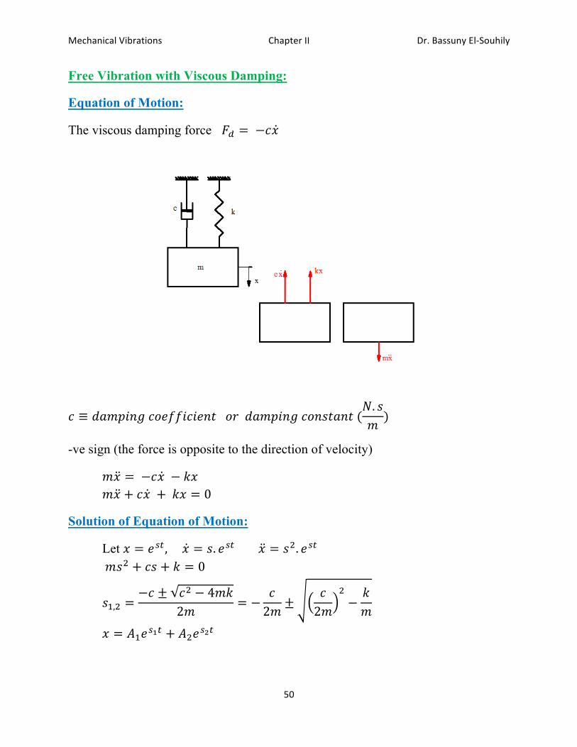
Free Vibration with Viscous Damping:
Equation of Motion:
The viscous damping force ÜK = %−A#%%%%%%
A ≡ 32"9;EF%A<:55;A;:EC%%%<1%%32"9;EF%A<E4C2EC%(W. 4")
-ve sign (the force is opposite to the direction of velocity)
"# = %−A# %− '# "# + A# %+ %'# = 0
Solution of Equation of Motion:
Let # = :LM,%%%%%# = 4. :LM%%%%%%%%# = 4,. :LM%%%%% %"4, + A4 + ' = 0%%%%%%%
4p,, =−A ± A, − 4"'
2"= −
A2"
±A2"
,−'"%%%%%%
# = sp:LàM + s,:L|M%%%
Dr.$Bassuny$El-Souhily$Chapter$II$Mechanical$Vibrations$$
51$$
A1 and A2 are arbitrary constants to be determined from the initial conditions of the system.
•! Critical damping coefficient cc is defined as the value of the damping constant c for which the radical in equation s1,2 becomes zero,
Aâ2"
,−'"= 0%%%
<1%Aâ = 2"'"= 2 '" = 2"*+
•! The damping factor or damping ratio ä%%
ä =AAâ%%
4p,, = −ä ± ä, − 1 *+%
# = sp:rãr ã|rp 67M + s,:
rãå ã|rp 67M
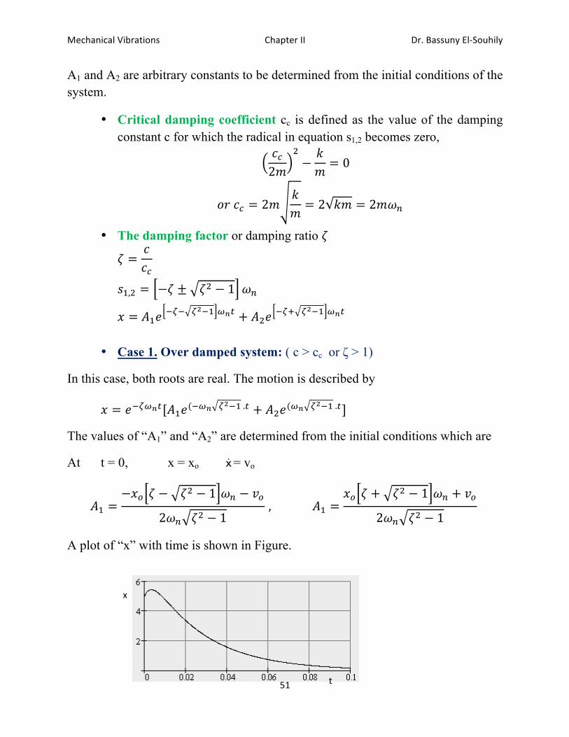
•! Case 1. Over damped system: ( c ˃ cc or ζ ˃ 1)
In this case, both roots are real. The motion is described by
# = :rã67M[sp:(r67 ã|rp%.M + s,:(67 ã|rp%.M]
The values of “A1” and “A2” are determined from the initial conditions which are
At t = 0, x = xo x! = vo
sp =−#T ä − ä, − 1 *+ − wT
2*+ ä, − 1%,%%%%%%%%%%%%%%sp =
#T ä + ä, − 1 *+ + wT
2*+ ä, − 1%
A plot of “x” with time is shown in Figure.
$$$
x$
t$
Dr.$Bassuny$El-Souhily$Chapter$II$Mechanical$Vibrations$$
52$$
No vibration The mass moves slowly back to the equilibrium position rather than vibrating about it.
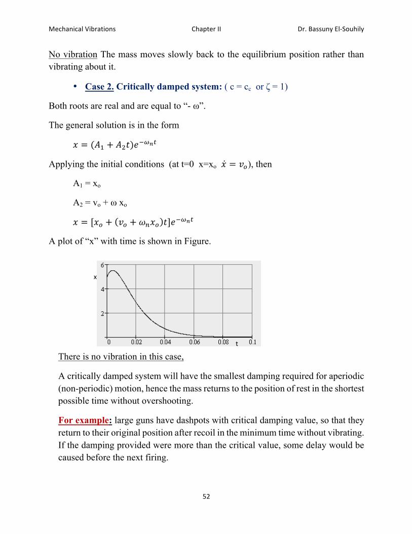
•! Case 2. Critically damped system: ( c = cc or ζ = 1)
Both roots are real and are equal to “- ω”.
The general solution is in the form
# = (sp + s,C):r67M
Applying the initial conditions (at t=0 x=xo # = wT), then
A1 = xo
A2 = vo + ω xo
# = [#T + wT + *+#T C]:r67M
A plot of “x” with time is shown in Figure.
There is no vibration in this case,
A critically damped system will have the smallest damping required for aperiodic (non-periodic) motion, hence the mass returns to the position of rest in the shortest possible time without overshooting.
For example: large guns have dashpots with critical damping value, so that they return to their original position after recoil in the minimum time without vibrating. If the damping provided were more than the critical value, some delay would be caused before the next firing.
$$$$
x$
t$
Dr.$Bassuny$El-Souhily$Chapter$II$Mechanical$Vibrations$$
53$$
•! Case 3. Under damped system: ( c ˂ cc or ζ ˂ 1)
In this case, both roots are complex and are given by
4p,, = −ä ± ; 1 − ä, *+%%%%
# = :rã67M[sp:(r67q prã|%.M + s,:(67q prã|%.M]
# = :rã67M[spç cos 1 − ä,*+C + s,
ç sin 1 − ä,*+C]
Let 1 − ä,*+ = *K%%%%%%%% Cℎ:%51:én:EAz%<5%Cℎ:%32"9:3%w;è12C;<E
# = :rã67M[spç cos*KC + s,
ç sin*KC]
The initial conditions which are at t = 0, x = xo x! = vo
# = :rã67M[#T cos*KC +ê^åã67x^
6ësin*KC]
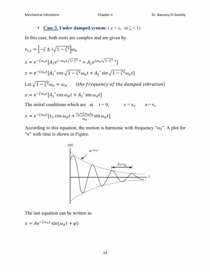
According to this equation, the motion is harmonic with frequency “ωd”. A plot for “x” with time is shown in Figure.
The last equation can be written as
# = s:rã67M sin(*KC + v)
Dr.$Bassuny$El-Souhily$Chapter$II$Mechanical$Vibrations$$
54$$
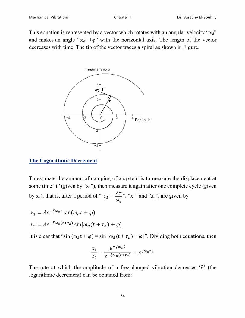
This equation is represented by a vector which rotates with an angular velocity “ωd”
and makes an angle “ωdt +φ” with the horizontal axis. The length of the vector decreases with time. The tip of the vector traces a spiral as shown in Figure.
$
The Logarithmic Decrement
To estimate the amount of damping of a system is to measure the displacement at some time “t” (given by “x1”), then measure it again after one complete cycle (given
by x2), that is, after a period of “ =K = d
2ω
π ”. “x1” and “x2”, are given by
#p = s:rã67M sin(*KC + v)
%#, = s:rã67(Måíë) sin[*K(C + =K) + v]
It is clear that “sin (ωd t + v) = sin [ωd (t + =K) + v]”. Dividing both equations, then
#p#,=
:rã67M
:rã67(Måíë)= :ã67íë
The rate at which the amplitude of a free damped vibration decreases ‘δ’ (the logarithmic decrement) can be obtained from:
r$
$
Real$axis$
Imaginary$axis$
$
Dr.$Bassuny$El-Souhily$Chapter$II$Mechanical$Vibrations$$
55$$
δ = ln 2
1
x
x= ä*+=K = ä*+
,8
6ë
= 21
2ζ−
ζπ
δ = p+DE xà
x7ìà
For small damping, δ ≈ 2πζ
Energy dissipated in viscous damping:
The rate of change of energy
3î3C
= 5<1A: ∗ w:D<A;Cz = Üw = −Aw, = −A(3#3C),
The negative sign, the energy dissipates with time
Assume # = ñ sin*KC (steady-state response under forced vibration)
Δò = A(3#3C),
,86ë
_3C = Añ,*K %cos, *KC%3*KC
,8
_= ?A*Kñ,
The fraction of energy of the vibrating system that is dissipated in each cycle,
Δòò
=?A*Kñ,
12"*K
,ñ,= 2%B = 4?ä = A<E4C2EC%%%
D<44%A<:55;A;:EC =ôö
,8ö
= ôö
,8ö ratio of energy dissipated per radian.
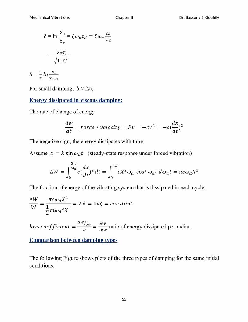
Comparison between damping types
The following Figure shows plots of the three types of damping for the same initial conditions.
Dr.$Bassuny$El-Souhily$Chapter$II$Mechanical$Vibrations$$
56$$
We notice that, for the over-damped system, the motion decays rather slowly without oscillations. The motion of critically damped systems is called “aperiodic”, or non periodic. The mass returns back to the equilibrium position without oscillation with the fastest rate. This type of damping is suitable for the recoil mechanism of guns. The gun barrel is required to return back after firing as fast as possible without oscillation. The case of under damping is used for applications which need to reduce vibrations.
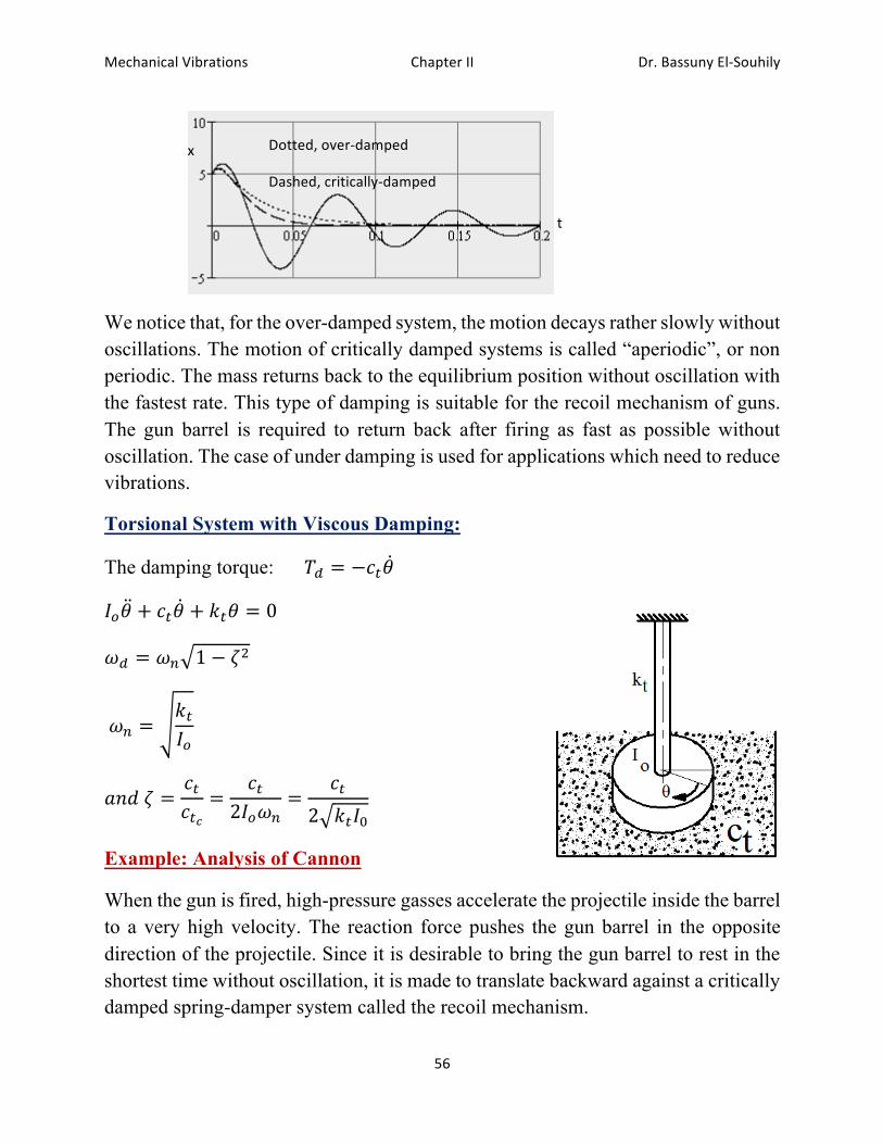
Torsional System with Viscous Damping:
The damping torque: NK = −AMZ%%%
YTZ + AMZ + 'MZ = 0%%%
*K = *+ 1 − ä,%%
%*+ ='MYT%%%%
2E3%ä =AMAMõ
=AM
2YT*+=
AM2 'MY_
Example: Analysis of Cannon
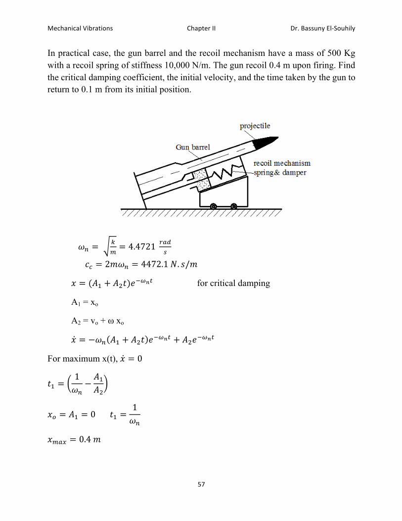
When the gun is fired, high-pressure gasses accelerate the projectile inside the barrel to a very high velocity. The reaction force pushes the gun barrel in the opposite direction of the projectile. Since it is desirable to bring the gun barrel to rest in the shortest time without oscillation, it is made to translate backward against a critically damped spring-damper system called the recoil mechanism.
Dotted,$over-damped$
Dashed,$critically-damped$
Solid,$under-damped$$
x$$
t$
$
Dr.$Bassuny$El-Souhily$Chapter$II$Mechanical$Vibrations$$
57$$
In practical case, the gun barrel and the recoil mechanism have a mass of 500 Kg with a recoil spring of stiffness 10,000 N/m. The gun recoil 0.4 m upon firing. Find the critical damping coefficient, the initial velocity, and the time taken by the gun to return to 0.1 m from its initial position.
*+ = %G
H= 4.4721% IJK
L%%
%Aâ = 2"*+ = 4472.1%W. 4/"
# = (sp + s,C):r67M for critical damping
A1 = xo
A2 = vo + ω xo
# = −*+ sp + s,C :r67M + s,:r67M
For maximum x(t), # = 0
Cp =1*+
−sps,
%%%%%%%%%%%%%%%%%%%%%%%%%%%%%%%%%%
#T = sp = 0%%%%%%%Cp =1*+%%%%
#HJx = 0.4%"%%
Dr.$Bassuny$El-Souhily$Chapter$II$Mechanical$Vibrations$$
58$$
#HJx = # C = Cp = % s,Cp :r67Mà =#T:*+
%
<1%#T = #HJx*+: = 4.8626"4%%%%
0.1 = %% s,C, :r67M|%%%%C, = 0.8258%4:A.%%
Free Vibration with Coulomb Damping “Dry Friction Damping”
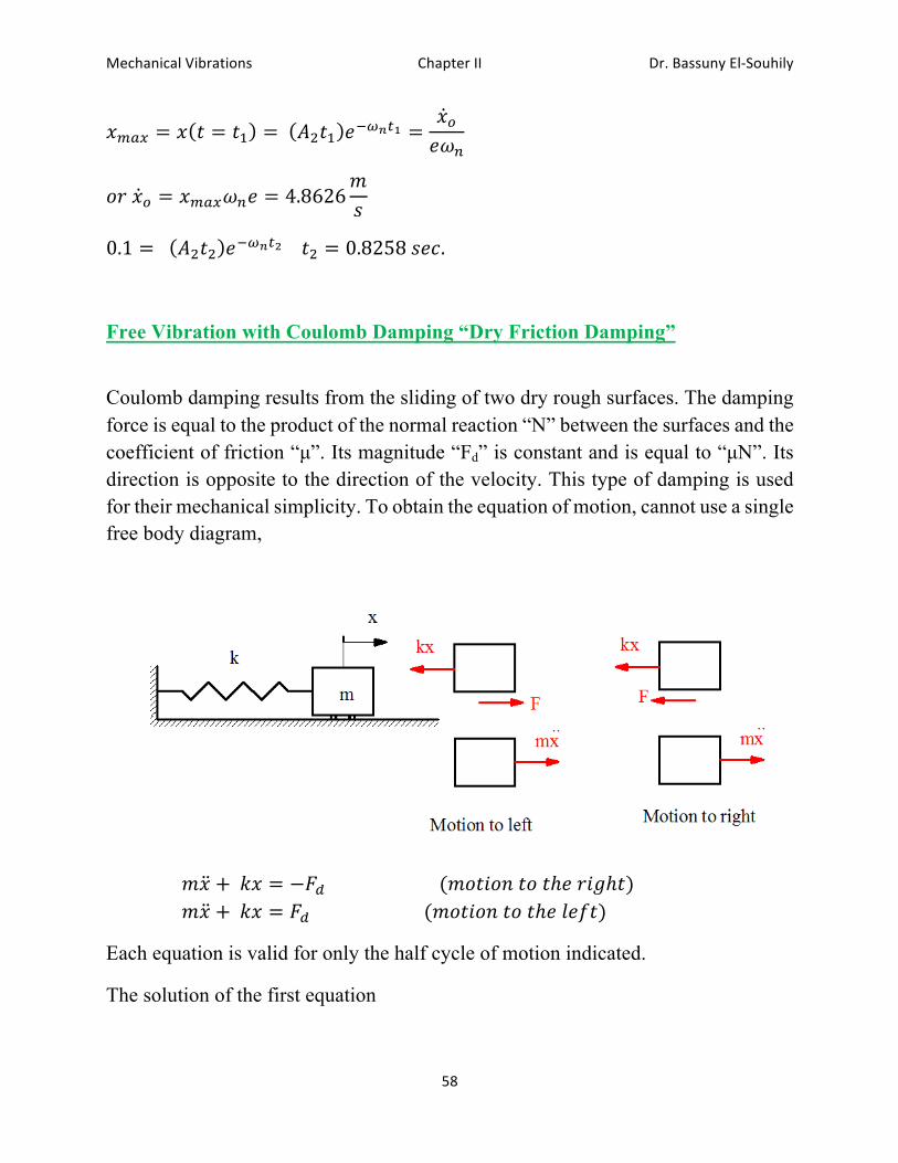
Coulomb damping results from the sliding of two dry rough surfaces. The damping force is equal to the product of the normal reaction “N” between the surfaces and the coefficient of friction “µ”. Its magnitude “Fd” is constant and is equal to “µN”. Its direction is opposite to the direction of the velocity. This type of damping is used for their mechanical simplicity. To obtain the equation of motion, cannot use a single free body diagram,
%%%%%"# + %'# = −ÜK%%%%%%%%%%%%%%%%%%%%%%%%%("<C;<E%C<%Cℎ:%1;FℎC) %%%%%"# + %'# = ÜK%%%%%%%%%%%%%%%%%%%%%%%%%("<C;<E%C<%Cℎ:%D:5C)
Each equation is valid for only the half cycle of motion indicated.
The solution of the first equation
Dr.$Bassuny$El-Souhily$Chapter$II$Mechanical$Vibrations$$
59$$
# = s cos*+C + t sin*+C −†W'
The solution of the second equation
# = u cos*+C + ° sin*+C +†W'
# = −s*+ sin*+C + t*+ cos*+C # = −u*+ sin*+C + °*+ cos*+C
This means that the system vibrates with a frequency which is equal to the natural frequency. The constants “A” , “B” , “C” and “D” are determined from the initial conditions.
Let at “t = 0”, x = xo and x! = vo
Let xo, x1, x2,… denote the amplitudes of motion at successive half cycles.
The constants are given by
u = #T − 3%%,%%%%%° = 0%%%%%%%%%%%%îℎ:1:%3 =†W'%%%%%%%%%%
# = (#T − 3) cos*+C + 3 The solution is valid for half the cycle only, i.e. for 0 ≤ t ≤ π/ω, when t=π/ω, the mass will be at its extreme left position and its displacement from equilibrium position can be found
−#p = # C =?*+
= #T − 3 cos ? + 3
%%%%%%%%%= −(#T − 23) The reduction in magnitude of x in time π/ω (half cycle) is 2d. In the second half cycle, the mass moves from left to right,
# C = 0 = w2Dn:%<5%#%2C%C =πω%%in%the%1¶ß%equation
%%%%%%%%%%%%%%%%%%= − #T − 23 %% 2E3%# = 0%% Nℎn4%% − s = −#T + 33,%%%%%%%t = 0%%%%% # = #T − 33 cos*+C − 3%%%% 2C%Cℎ:%:E3%<5%Cℎ;4%ℎ2D5%AzAD:%,%
Dr.$Bassuny$El-Souhily$Chapter$II$Mechanical$Vibrations$$
60$$
#, = (#%2C C =?*+
= #T − 43 %
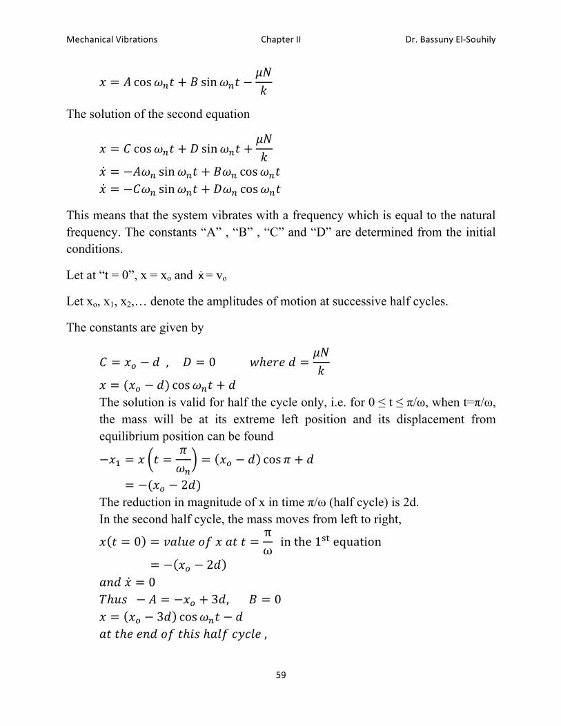
2E3%# = 0%%% These become the initial condition of the third half cycle. •! The motion stops when xn ≤ d, since the restoring force exerted by the
spring force (kx) will then be less than the friction force (µN). •! The number of half cycles (r) that elapse before the motion ceases is given
by,
#T − 1. 3 ≤ 3%%%%%%%%%%%Cℎ2C%;4%%%%%%%1 ≥ {#T − 323
}
The total motion is described by the Figure shown,
It is clear that the amplitude decreases with a constant rate.
ωnt$
x$
$
d$
$
$
$
$
$
$
$
-d$
$
$
$
Imaginary$axis$
$
$
$
Real$axis$
Dr.$Bassuny$El-Souhily$Chapter$II$Mechanical$Vibrations$$
61$$
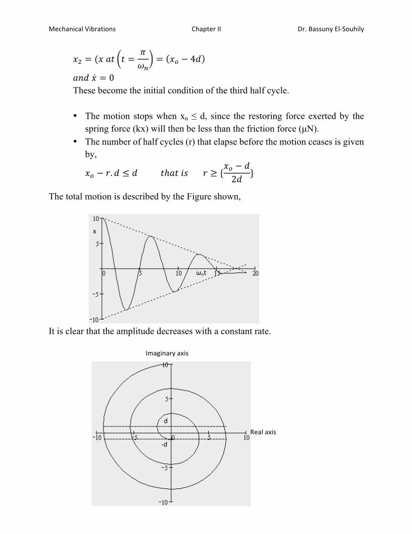
The vector plot is a half a circle with radius “xmax – d” and center at “0, d” located at the left side of the imaginary axis. Similarly, the vector plot located at the right side of the imaginary axis is a half a circle with radius “xmin + d” and center at “0, -d”.
Notes
1-!The equation of motion is nonlinear, 2-!The natural frequency is not changed with Coulomb damping, 3-!The motion is periodic, 4-!The system comes to rest after some time, theoretically continuous forever
with viscous damping, 5-!The amplitude reduces linearly (exponentially in viscous damping), 6-! In each successive cycle, the amplitude is reduced by 4d
#H = #Hrp −4†W'
The slope of the enveloping straight lines shown
−
4†W'2?*+
= %−2†W*+?'
7-! Potential energy,
O+ − O+åp =12'#+, −
12'#+åp, %%%= %ÜK #+ + #+åp %
%%%%%%%%%%%%%%%%%%%%%%%%%12' #+, − #+åp,% %= %ÜK #+ + #+åp %%%
p,' #+ − #+åp% %= %ÜK%%%%
%%%%%%%%%%%%%%%%%%%%%%%%%%%%%%%%% #+ − #+åp% %=2ÜK%'
= 23%%%%%%%25C:1%ℎ2D5%AzAD:%%%%%
%%%%%%%%%%%%%%%%%%%%%%%%%%%%%%%%%%%%%%5<1%:2Aℎ%AzAD: = 43
Example: “Pulley subjected to Coulomb damping”
A steel shaft of length 1 m and diameter 50 mm is fixed at one end and carries a pulley of mass moment of inertia 25 Kg.m2 at the other end. A band brake exerts a constant frictional torque of 400 N.m around the circumference of the pulley. If the pulley is displaced by 6o and released, determine: i- the number of cycles before the pulley comes to rest and ii- the final setting position of the pulley.
Dr.$Bassuny$El-Souhily$Chapter$II$Mechanical$Vibrations$$
62$$
Solution:
The number of half cycles that elapse before the angular motion of the pulley ceases is:
%%%%1 ≥ZT − 323
%%%%%%%%%%%3 =NK'M%%%
%%%ZT = 6T = 0.10472%123.%%%%%%%%%
%%%'M =RSD= 49,087.5%%
W."123
%%%%%
%%NK = 400%W."%%%%%%%%
%%∴ 1 = 5.926%%%
Cℎn4%Cℎ:%"<C;<E%A:24:4%25C:1%6%ℎ2D5%AzAD:4.
The angular displacement after 6 half cycles
Z = 0.10472 − 6 ∗ 2400
49,087.5
%%%%= 0.006935%%123. = 0.39734T
Thus the pulley stops at 0.39734o from the equilibrium position on the same side of the initial displacement.