Frank Edward Curtis Northwestern University Joint work with Richard Byrd and Jorge Nocedal February...
74
Frank Edward Curtis Northwestern University Joint work with Richard Byrd and Jorge Nocedal February 12, 2007 Inexact Methods for PDE- Constrained Optimization Emory University
-
Upload
tiffany-flowers -
Category
Documents
-
view
216 -
download
1
Transcript of Frank Edward Curtis Northwestern University Joint work with Richard Byrd and Jorge Nocedal February...
Frank Edward CurtisNorthwestern University
Joint work with Richard Byrd and Jorge Nocedal
February 12, 2007
Inexact Methods for PDE-Constrained Optimization
Emory University
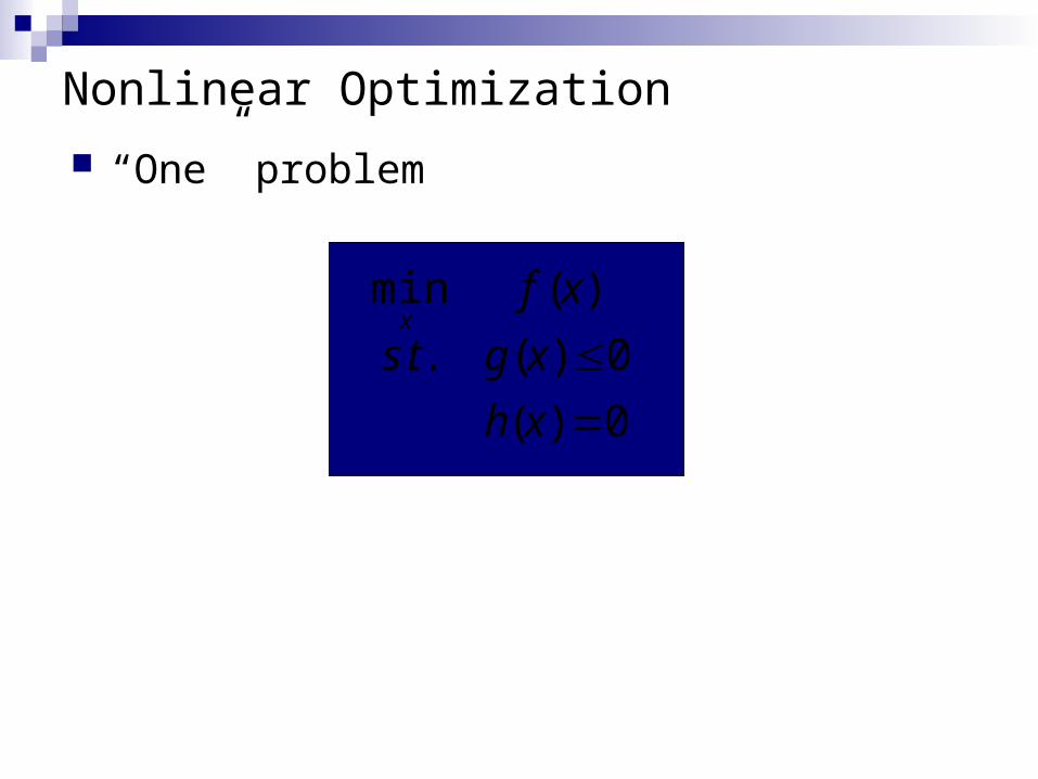
Nonlinear Optimization
“One” problem
0)(
0)(..
)(min
xh
xgts
xfx
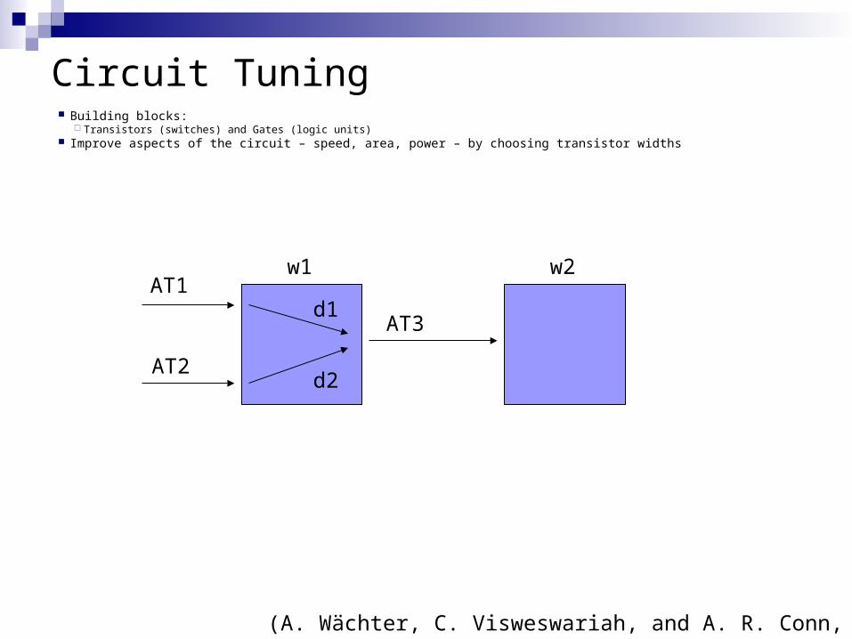
Circuit Tuning Building blocks:
Transistors (switches) and Gates (logic units) Improve aspects of the circuit – speed, area, power – by choosing transistor widths
AT1
AT3
AT2
d1
d2
w1 w2
(A. Wächter, C. Visweswariah, and A. R. Conn, 2005)
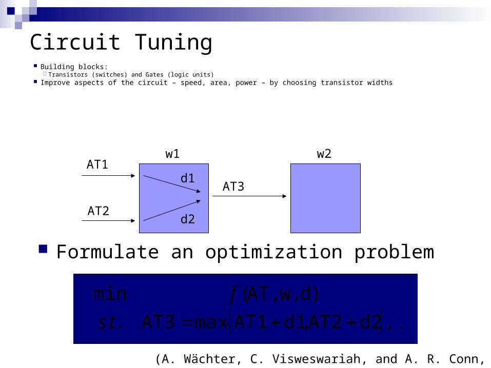
Circuit Tuning Building blocks:
Transistors (switches) and Gates (logic units) Improve aspects of the circuit – speed, area, power – by choosing transistor widths
Formulate an optimization problem
,...d2AT2,d1AT1maxAT3..
)dw,AT,(min
ts
f
AT1
AT3
AT2
d1
d2
w1 w2
(A. Wächter, C. Visweswariah, and A. R. Conn, 2005)

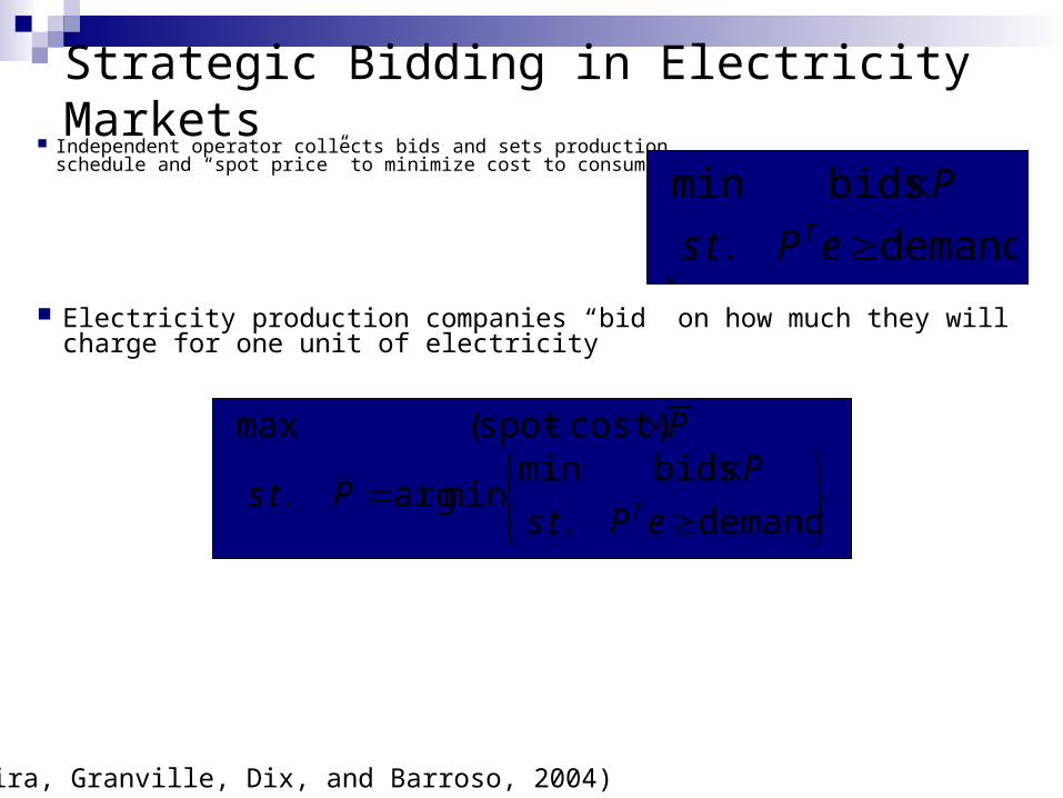
Strategic Bidding in Electricity Markets Independent operator collects bids and sets production
schedule and “spot price” to minimize cost to consumers
(Pereira, Granville, Dix, and Barroso, 2004)
demand..
bidsmin
ePts
PT
Strategic Bidding in Electricity Markets Independent operator collects bids and sets production
schedule and “spot price” to minimize cost to consumers
demand..
bidsminminarg..
cost)spot(max
ePts
PPts
P
T
(Pereira, Granville, Dix, and Barroso, 2004)
demand..
bidsmin
ePts
PT
Electricity production companies “bid” on how much they will charge for one unit of electricity
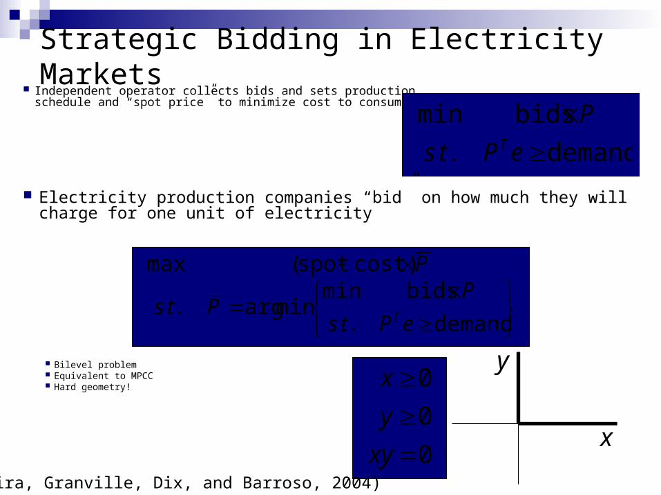
Strategic Bidding in Electricity Markets Independent operator collects bids and sets production
schedule and “spot price” to minimize cost to consumers
demand..
bidsminminarg..
cost)spot(max
ePts
PPts
P
T
0
0
0
xy
y
x Bilevel problem Equivalent to MPCC Hard geometry!
y
x
(Pereira, Granville, Dix, and Barroso, 2004)
demand..
bidsmin
ePts
PT
Electricity production companies “bid” on how much they will charge for one unit of electricity

Challenges for NLP algorithms Very large problems Numerical noise Availability of derivatives Degeneracies Difficult geometries Expensive function evaluations Real-time solutions needed Integer variables Negative curvature
Outline Problem Formulation
Equality constrained optimization Sequential Quadratic Programming
Inexact Framework Unconstrained optimization and nonlinear equations Stopping conditions for linear solver
Global Behavior Merit function and sufficient decrease Satisfying first order conditions
Numerical Results Model inverse problem Accuracy tradeoffs
Final Remarks Future work Negative curvature

Equality constrained optimization
e.g., minimize the difference between observed and expected behavior, subject to atmospheric flow equations (Navier-Stokes)
Goal: solve the problem
0)(s.t.
)(min
xcxf
x
*x
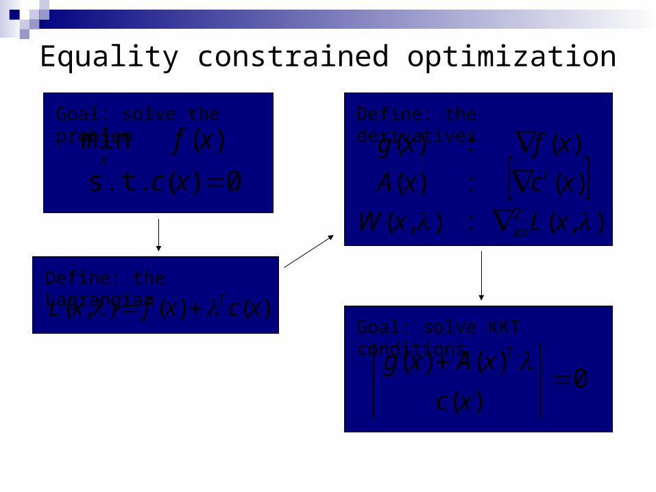
Goal: solve the problem
Equality constrained optimization
)()(),( xcxfxL T
0)(s.t.
)(min
xcxf
x ),(:),(
)(:)(
)(:)(
2 xLxW
xcxA
xfxg
xx
i
0)(
)()(
xc
xAxg T
Define: the Lagrangian
Define: the derivatives
Goal: solve KKT conditions
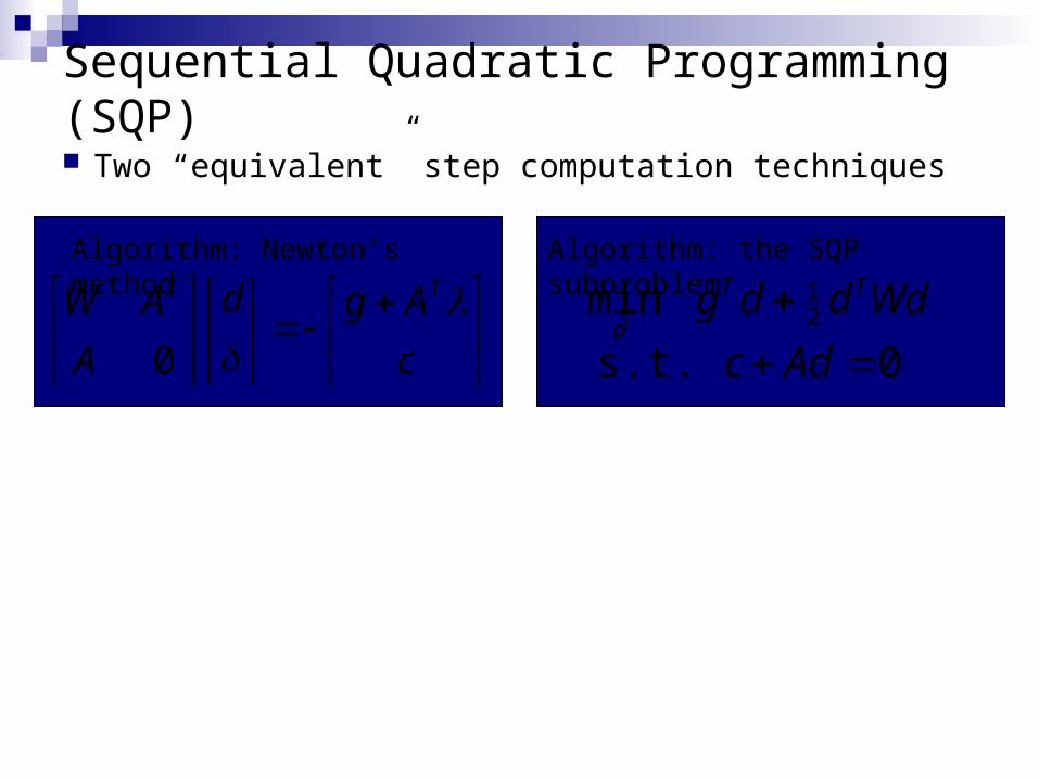
Sequential Quadratic Programming (SQP)
0s.t.
min 21
Adc
Wdddg TT
d
c
Agd
A
AW TT 0
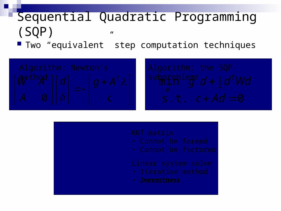
Algorithm: Newton’s method
Algorithm: the SQP subproblem
Two “equivalent” step computation techniques

Sequential Quadratic Programming (SQP)
c
Agd
A
AW TT 0 0s.t.
min 21
Adc
Wdddg TT
d
Algorithm: Newton’s method
Algorithm: the SQP subproblem
Two “equivalent” step computation techniques
0A
AW T KKT matrix• Cannot be formed• Cannot be factored
Sequential Quadratic Programming (SQP)
c
Agd
A
AW TT 0 0s.t.
min 21
Adc
Wdddg TT
d
Algorithm: Newton’s method
Algorithm: the SQP subproblem
Two “equivalent” step computation techniques
0A
AW T KKT matrix• Cannot be formed• Cannot be factored
Linear system solve• Iterative method• Inexactness

Outline Problem Formulation
Equality constrained optimization Sequential Quadratic Programming
Inexact Framework Unconstrained optimization and nonlinear equations Stopping conditions for linear solver
Global Behavior Merit function and sufficient decrease Satisfying first order conditions
Numerical Results Model inverse problem Accuracy tradeoffs
Final Remarks Future work Negative curvature

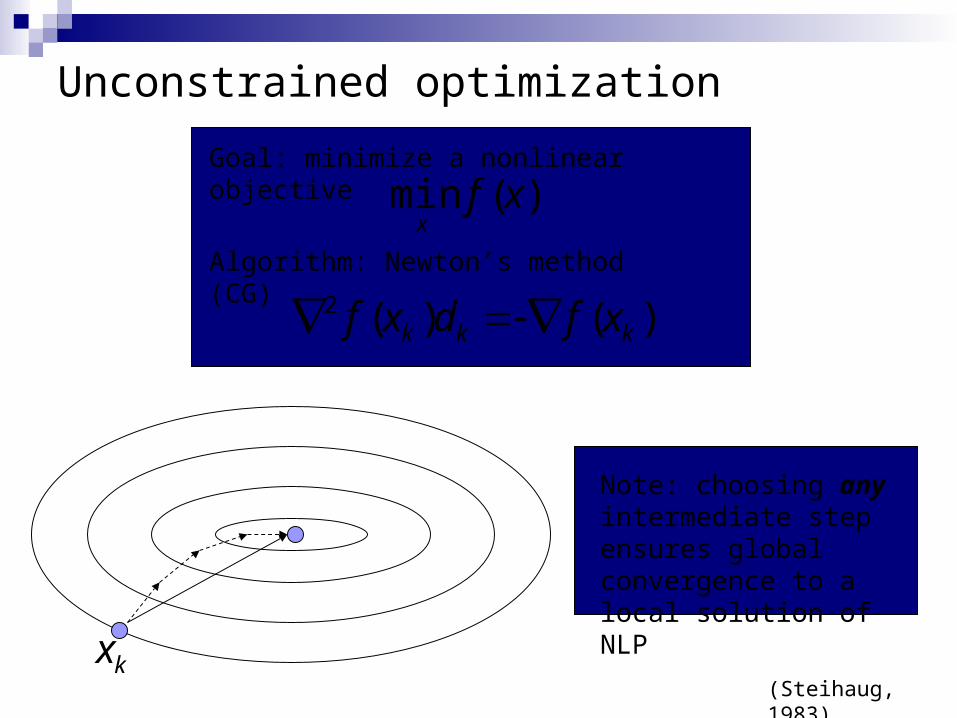
Unconstrained optimization
)(min xfx
)()(2kkk xfdxf
Goal: minimize a nonlinear objective
Algorithm: Newton’s method (CG)
Unconstrained optimization
)(min xfx
kx
)()(2kkk xfdxf
Goal: minimize a nonlinear objective
Algorithm: Newton’s method (CG)
Note: choosing any intermediate step ensures global convergence to a local solution of NLP
(Steihaug, 1983)
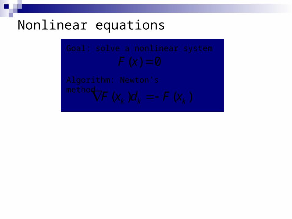
Nonlinear equations
0)( xF
)()( kkk xFdxF
Goal: solve a nonlinear system
Algorithm: Newton’s method

any step with
and
ensures descent
Nonlinear equations
kkkk rxFdxF )()(
0)( xF
kx
)()( kkk xFdxF
Goal: solve a nonlinear system
Algorithm: Newton’s method
10 ,)( kk xFr
(Eisenstat and Walker, 1994)
(Dembo, Eisenstat, and Steihaug, 1982)
0s.t.
min 21
Adc
Wdddg TT
d
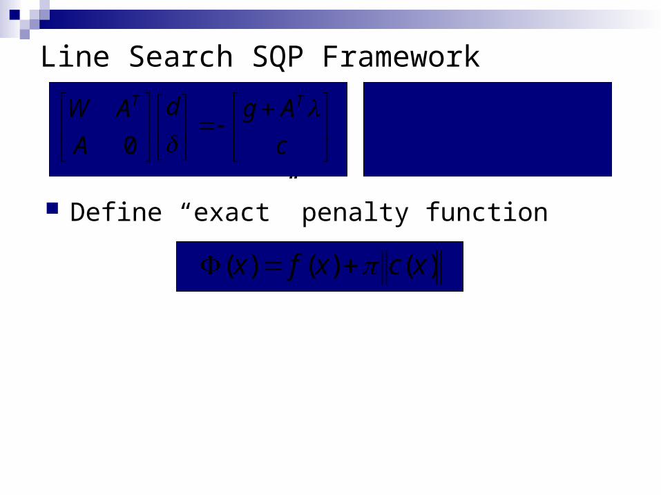
)()()( xcxfx
Line Search SQP Framework
Define “exact” penalty function
c
Agd
A
AW TT 0

0s.t.
min 21
Adc
Wdddg TT
d
)()()( xcxfx
Line Search SQP Framework
Define “exact” penalty function
c
Agd
A
AW TT 0
)( dx
1
)( dx
10

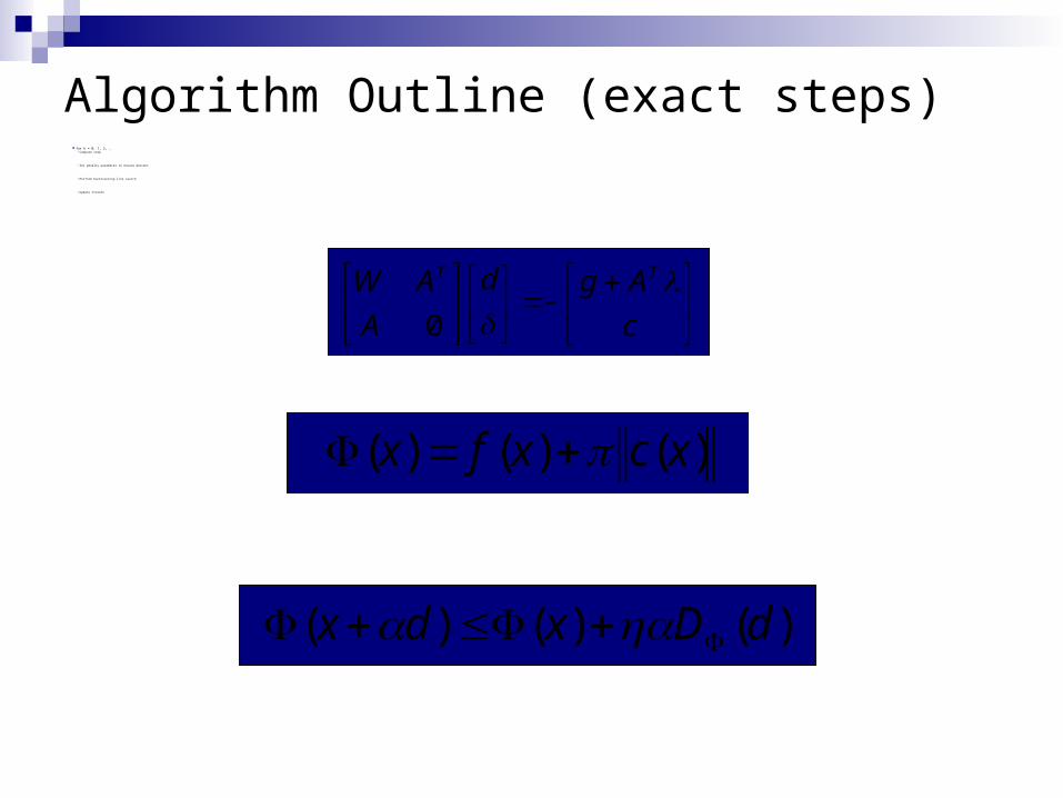
for k = 0, 1, 2, … Compute step by…
Set penalty parameter to ensure descent on…
Perform backtracking line search to satisfy…
Update iterate
Algorithm Outline (exact steps)
c
Agd
A
AW TT 0
)()()( xcxfx
)()()( dDxdx
0s.t.
min 21
Adc
Wdddg TT
d
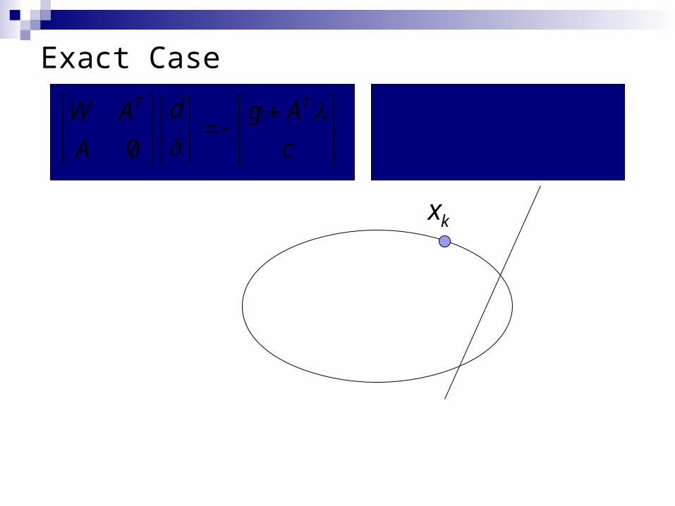
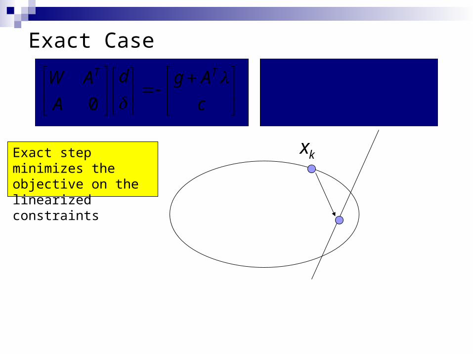
Exact Case
kx
c
Agd
A
AW TT 0
0s.t.
min 21
Adc
Wdddg TT
d
Exact Case
Exact step minimizes the objective on the linearized constraints
kx
c
Agd
A
AW TT 0

0s.t.
min 21
Adc
Wdddg TT
d
Exact Case
kxExact step minimizes the objective on the linearized constraints
… which may lead to an increase in the model objective
c
Agd
A
AW TT 0
)(
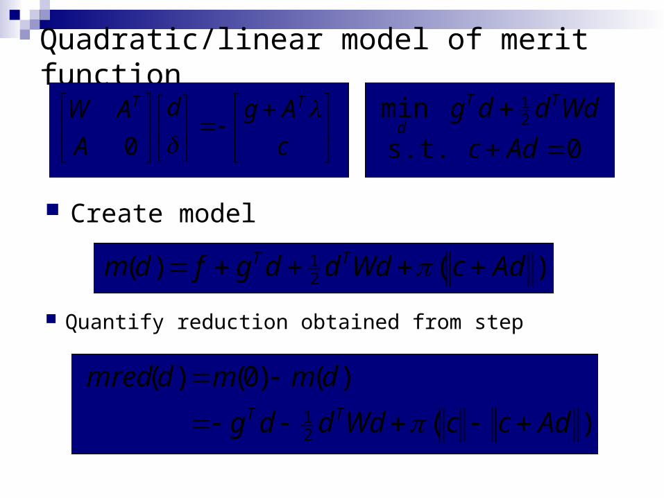
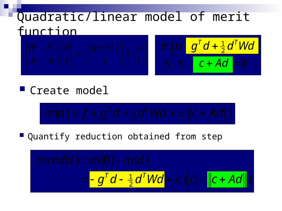
)()0()(
21 AdccWdddg
dmmdmredTT
)()( 21 AdcWdddgfdm TT
Quadratic/linear model of merit function
Create model
Quantify reduction obtained from step
0s.t.
min 21
Adc
Wdddg TT
d
c
Agd
A
AW TT 0
)()( 21 AdcWdddgfdm TT
Quadratic/linear model of merit function
Create model
Quantify reduction obtained from step
0s.t.
min 21
Adc
Wdddg TT
d
)(
)()0()(
21 AdccWdddg
dmmdmredTT
rc
Agd
A
AW TT 0

0s.t.
min 21
Adc
Wdddg TT
d
Exact Case
kxExact step minimizes the objective on the linearized constraints
… which may lead to an increase in the model objective
c
Agd
A
AW TT 0
0s.t.
min 21
Adc
Wdddg TT
d
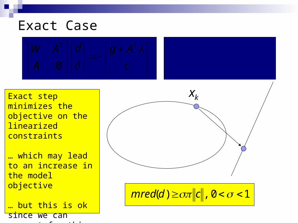
Exact Case
kx
10 ,)( cdmred
c
Agd
A
AW TT 0
Exact step minimizes the objective on the linearized constraints
… which may lead to an increase in the model objective
… but this is ok since we can account for this conflict by increasing the penalty parameter

0s.t.
min 21
Adc
Wdddg TT
d
Exact Case
kxExact step minimizes the objective on the linearized constraints
… which may lead to an increase in the model objective
… but this is ok since we can account for this conflict by increasing the penalty parameter
10 ,)1(
21
c
Wdddg TT
c
Agd
A
AW TT 0

for k = 0, 1, 2, … Compute step by…
Set penalty parameter to ensure descent on…
Perform backtracking line search to satisfy…
Update iterate
Algorithm Outline (exact steps)
c
Agd
A
AW TT 0
)()()( xcxfx
)()()( dDxdx
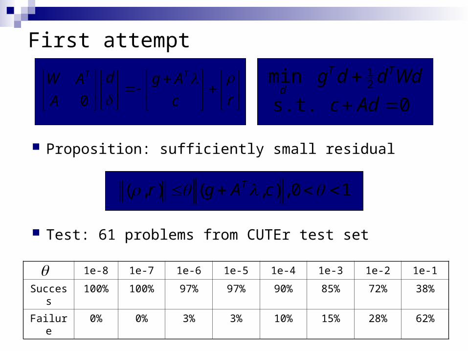
First attempt
10 ,),(),( cAgr T
Proposition: sufficiently small residual
1e-8 1e-7 1e-6 1e-5 1e-4 1e-3 1e-2 1e-1
Success 100% 100% 97% 97% 90% 85% 72% 38%
Failure 0% 0% 3% 3% 10% 15% 28% 62%
Test: 61 problems from CUTEr test set
0s.t.
min 21
Adc
Wdddg TT
d
rc
Agd
A
AW TT 0
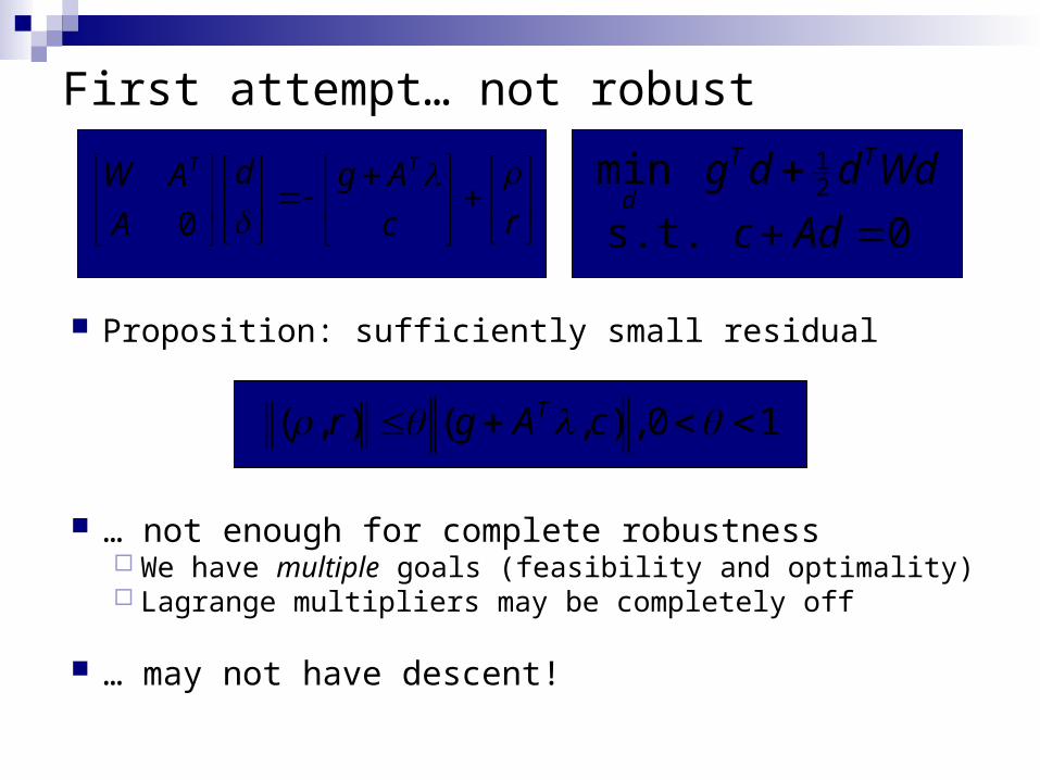
First attempt… not robust
10 ,),(),( cAgr T
Proposition: sufficiently small residual
0s.t.
min 21
Adc
Wdddg TT
d
rc
Agd
A
AW TT 0
… not enough for complete robustness We have multiple goals (feasibility and optimality) Lagrange multipliers may be completely off
… may not have descent!

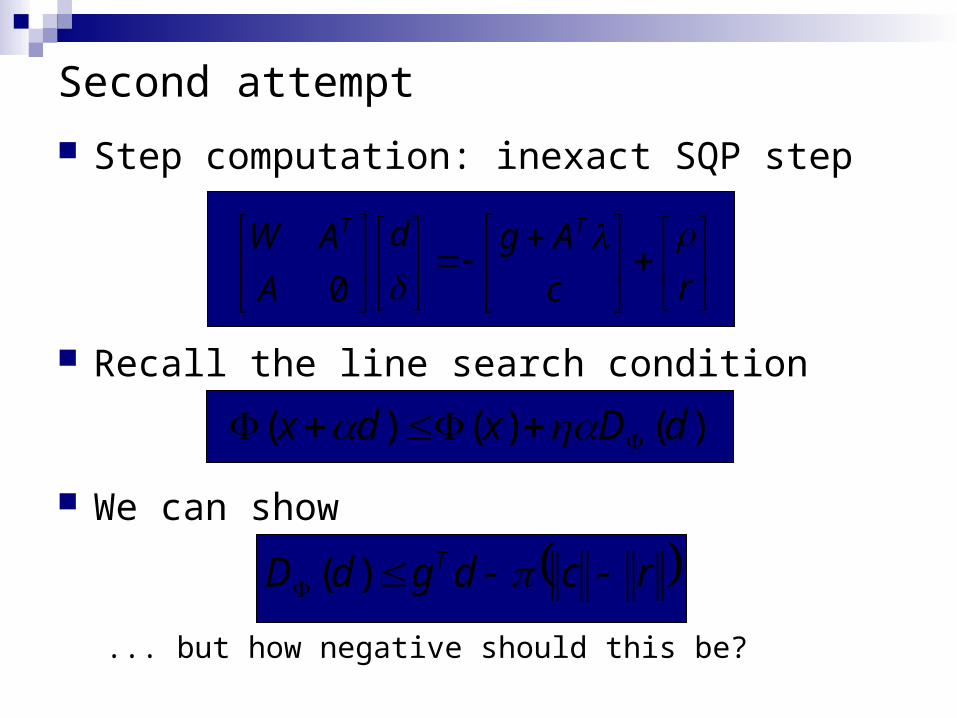
Recall the line search condition
Second attempt
rcdgdD T )(
Step computation: inexact SQP step
)()()( dDxdx
rc
Agd
A
AW TT 0
We can show
Recall the line search condition
Second attempt
rcdgdD T )(
Step computation: inexact SQP step
)()()( dDxdx
rc
Agd
A
AW TT 0
We can show
... but how negative should this be?
for k = 0, 1, 2, … Compute step
Set penalty parameter to ensure descent
Perform backtracking line search
Update iterate
Algorithm Outline (exact steps)
c
Agd
A
AW TT 0
)()()( xcxfx
)()()( dDxdx
for k = 0, 1, 2, … Compute step and set penalty parameter to ensure descent and a stable algorithm
Perform backtracking line search
Update iterate
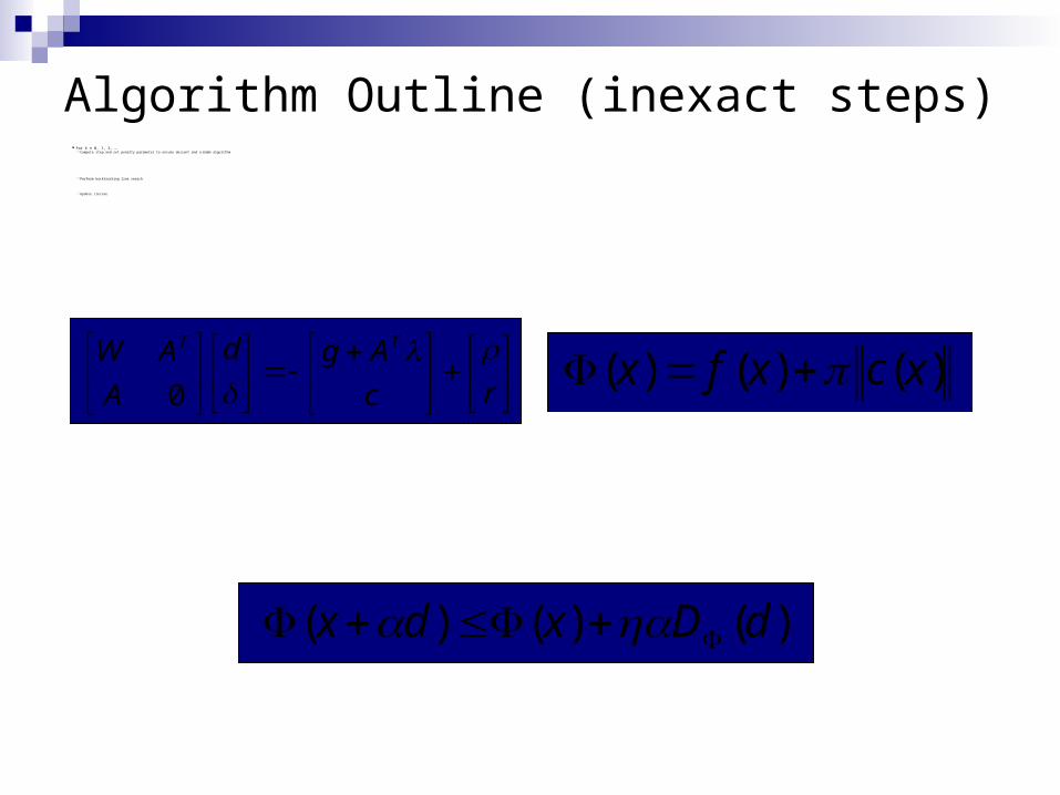
Algorithm Outline (inexact steps)
rc
Agd
A
AW TT 0
)()()( xcxfx
)()()( dDxdx
0s.t.
min 21
Adc
Wdddg TT
d
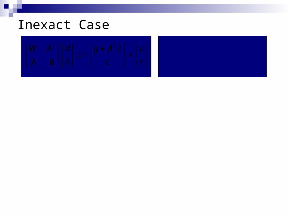
Inexact Case
rc
Agd
A
AW TT 0
crcWdddg TT 21
0s.t.
min 21
Adc
Wdddg TT
d
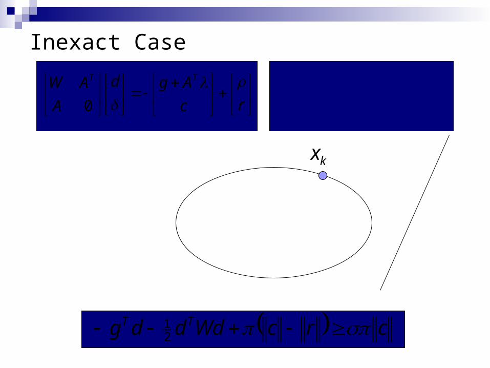
Inexact Case
rc
Agd
A
AW TT 0
kx
0s.t.
min 21
Adc
Wdddg TT
d
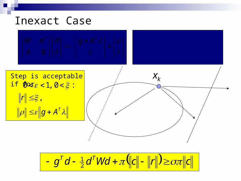
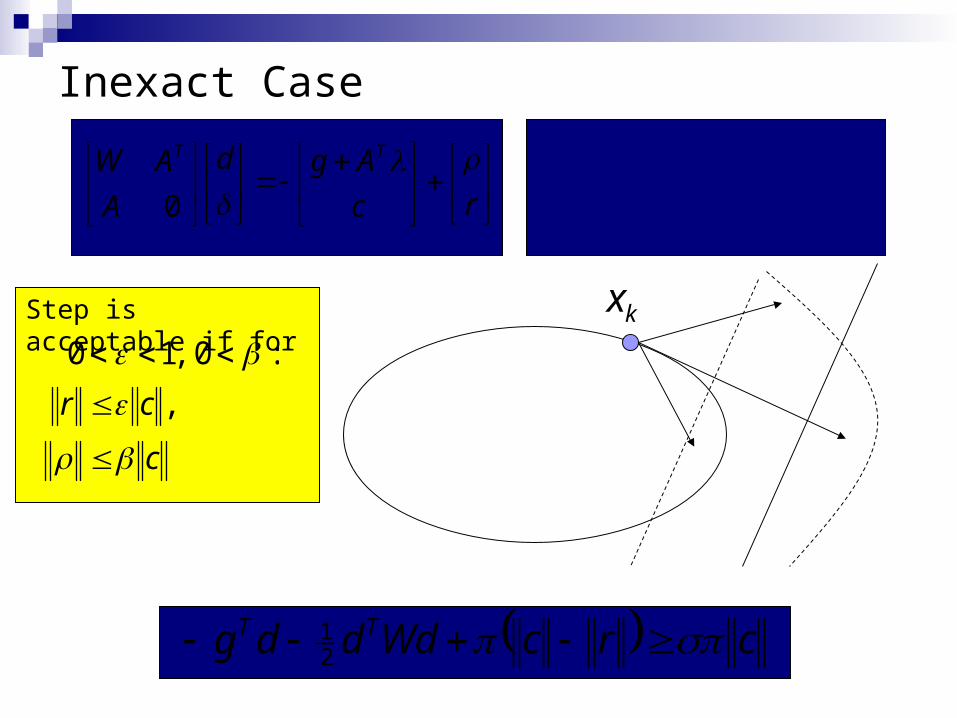
Inexact Case
rc
Agd
A
AW TT 0
kx
TAg
r
,
:0 ,10Step is acceptable if for
crcWdddg TT 21
0s.t.
min 21
Adc
Wdddg TT
d
Inexact Case
rc
Agd
A
AW TT 0
kx
c
cr
,
:0 ,10
Step is acceptable if for
crcWdddg TT 21
0s.t.
min 21
Adc
Wdddg TT
d
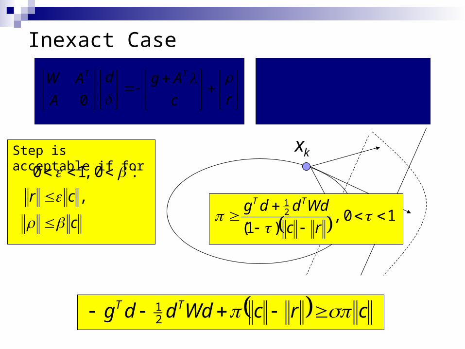
Inexact Case
rc
Agd
A
AW TT 0
kx
c
cr
,
:0 ,10
Step is acceptable if for
10 ,)1(
21
rc
Wdddg TT
crcWdddg TT 21
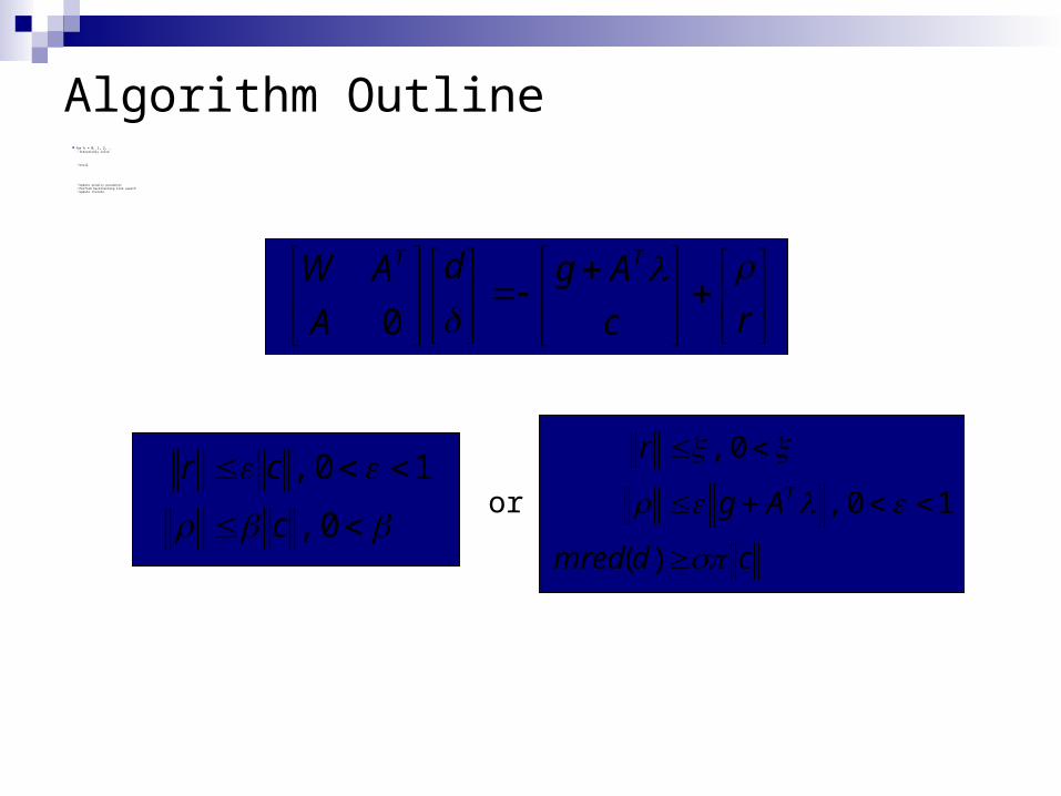
for k = 0, 1, 2, … Iteratively solve
Until
Update penalty parameter Perform backtracking line search Update iterate
Algorithm Outline
cdmred
Ag
rT
)(
10 ,
0 ,
0 ,
10 ,
c
cr
rc
Agd
A
AW TT 0
or
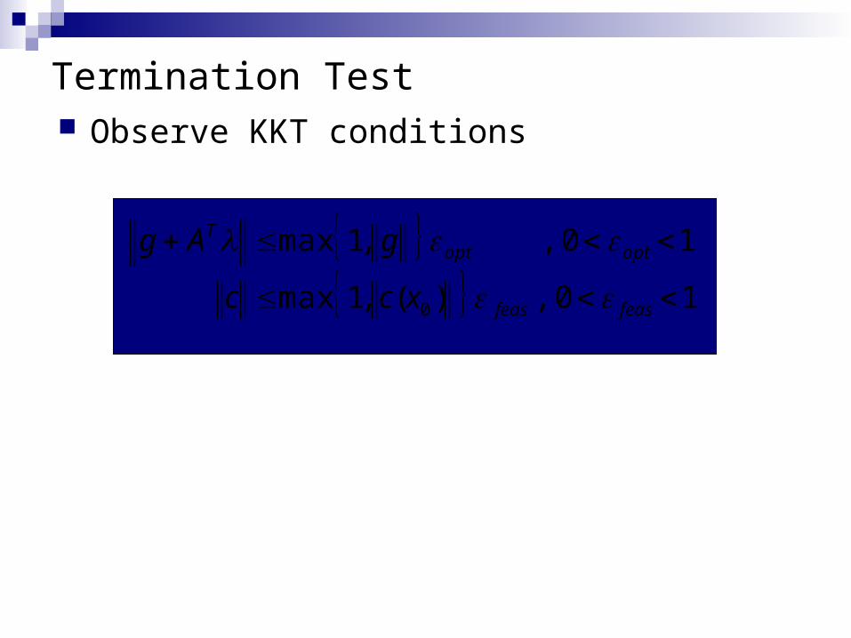
Observe KKT conditions
Termination Test
10 , )(,1 max
10 , ,1 max
0
feasfeas
optoptT
xcc
gAg
Outline Problem Formulation
Equality constrained optimization Sequential Quadratic Programming
Inexact Framework Unconstrained optimization and nonlinear equations Stopping conditions for linear solver
Global Behavior Merit function and sufficient decrease Satisfying first order conditions
Numerical Results Model inverse problem Accuracy tradeoffs
Final Remarks Future work Negative curvature

The sequence of iterates is contained in a convex set and the following conditions hold:
the objective and constraint functions and their first and second derivatives are bounded the multiplier estimates are bounded the constraint Jacobians have full row rank and their smallest singular values are bounded below by a positive constant the Hessian of the Lagrangian is positive definite with smallest eigenvalue bounded below by a positive constant
Assumptions
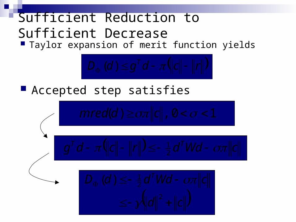
Sufficient Reduction to Sufficient Decrease
rcdgdD T )(
cWddrcdg TT 21
cd
cWdddD T
2
21)(
10 ,)( cdmred
Taylor expansion of merit function yields
Accepted step satisfies

Intermediate Results
0 ,
10 ,
c
cr
10 ,)1(
21
rc
Wdddg TT
cdmred
Ag
rT
)(
0 ,
0 ,
d
is bounded below by a positive constant
is bounded above
is bounded above

Sufficient Decrease in Merit Function
cdxdD 2
),;(
0lim k
Tk
kgZ
0lim2
kkk
cd
cddxx 2);();(
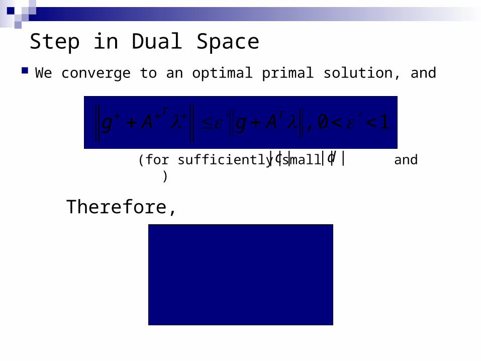
Step in Dual Space
10 , TTAgAg
|||| c |||| d(for sufficiently small and )
0lim k
kc
0lim k
Tkk
kAg
Therefore,
We converge to an optimal primal solution, and

Outline Problem Formulation
Equality constrained optimization Sequential Quadratic Programming
Inexact Framework Unconstrained optimization and nonlinear equations Stopping conditions for linear solver
Global Behavior Merit function and sufficient decrease Satisfying first order conditions
Numerical Results Model inverse problem Accuracy tradeoffs
Final Remarks Future work Negative curvature
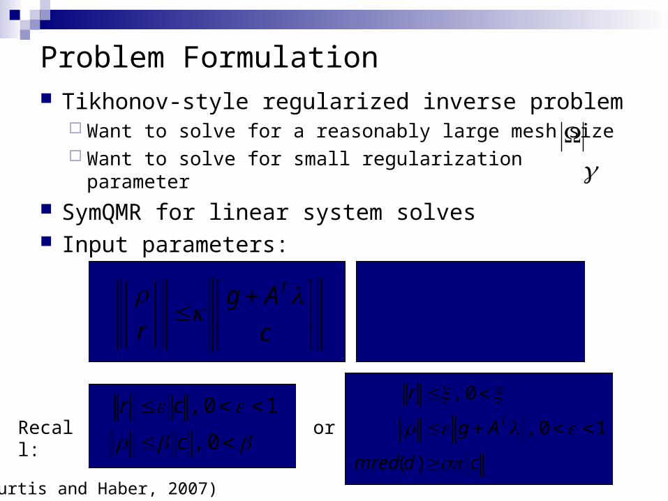
Problem Formulation Tikhonov-style regularized inverse problem
Want to solve for a reasonably large mesh size Want to solve for small regularization parameter
SymQMR for linear system solves Input parameters:
c
Ag
r
T
0.1 ,1
,1 ,1.0
cdmred
Ag
rT
)(
10 ,
0 ,
0 ,
10 ,
c
crorRecall
:
(Curtis and Haber, 2007)
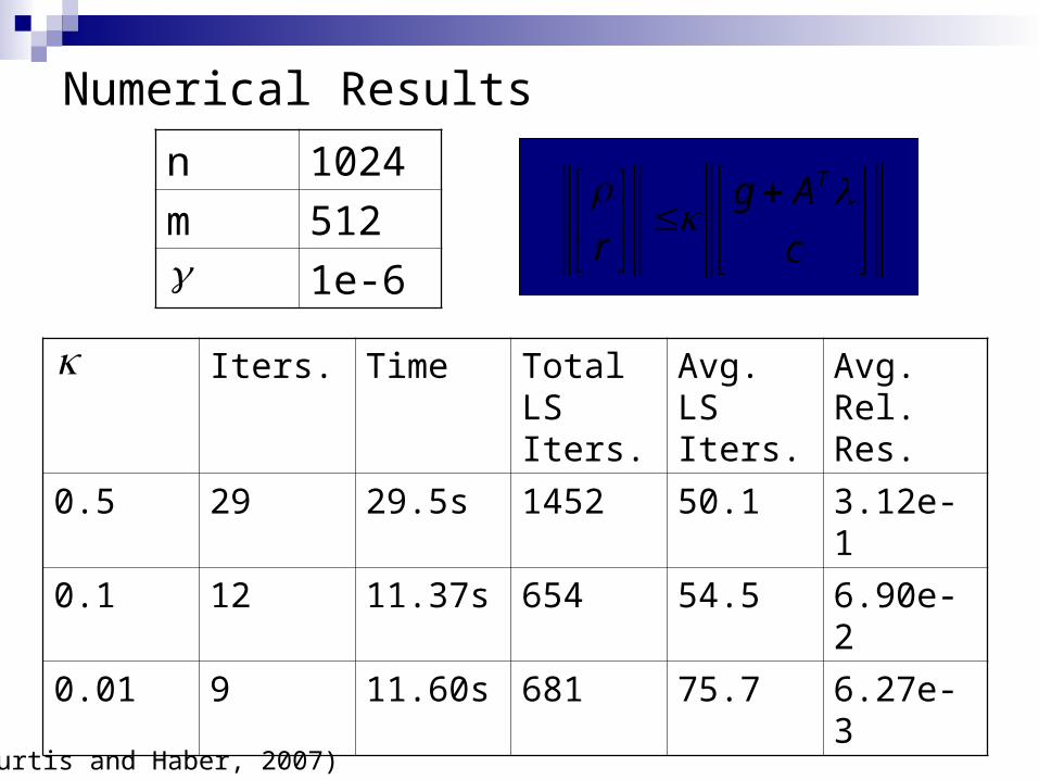
Numerical Results
c
Ag
r
T
Iters. Time Total LS Iters.
Avg. LS Iters.
Avg. Rel. Res.
0.5 29 29.5s 1452 50.1 3.12e-1
0.1 12 11.37s 654 54.5 6.90e-2
0.01 9 11.60s 681 75.7 6.27e-3
n 1024
m 512
1e-6
(Curtis and Haber, 2007)
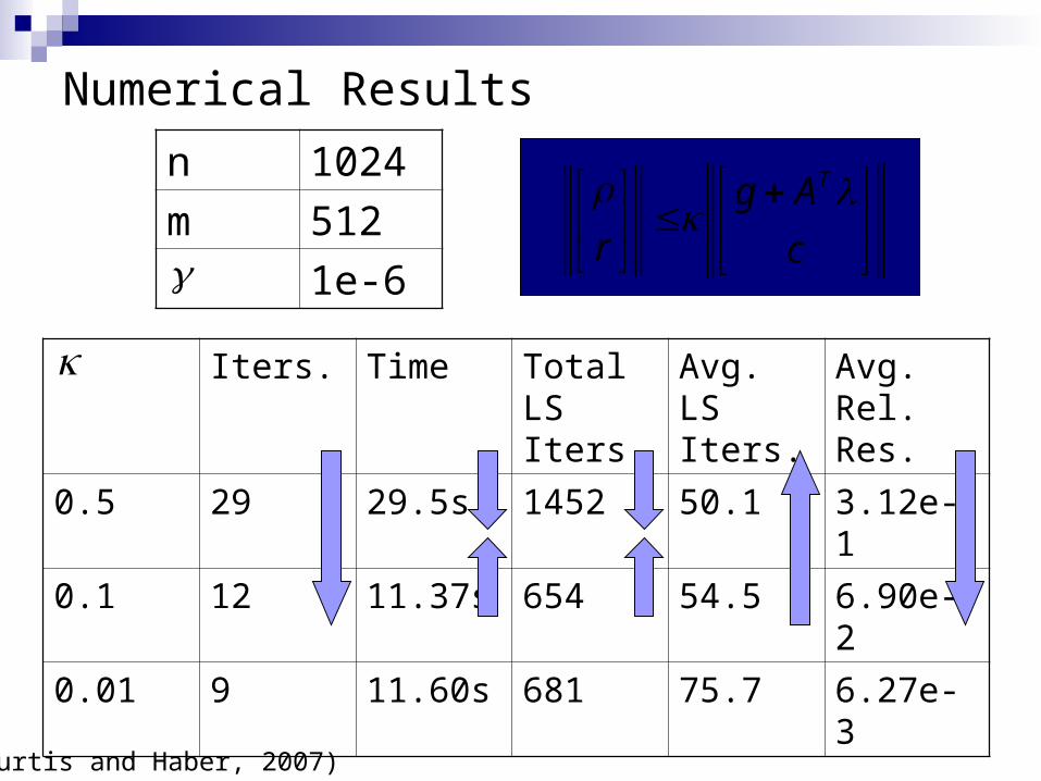
Numerical Results
c
Ag
r
T
Iters. Time Total LS Iters.
Avg. LS Iters.
Avg. Rel. Res.
0.5 29 29.5s 1452 50.1 3.12e-1
0.1 12 11.37s 654 54.5 6.90e-2
0.01 9 11.60s 681 75.7 6.27e-3
n 1024
m 512
1e-6
(Curtis and Haber, 2007)

Numerical Results
Iters. Time Total LS Iters.
Avg. LS Iters.
Avg. Rel. Res.
1e-6 12 11.40s 654 54.5 6.90e-2
1e-7 11 14.52s 840 76.4 6.99e-2
1e-8 8 10.57s 639 79.9 6.15e-2
1e-9 11 18.52s 1139 104 8.65e-2
1e-10 19 44.41s 2708 143 8.90e-2
n 1024
m 512
1e-1
(Curtis and Haber, 2007)
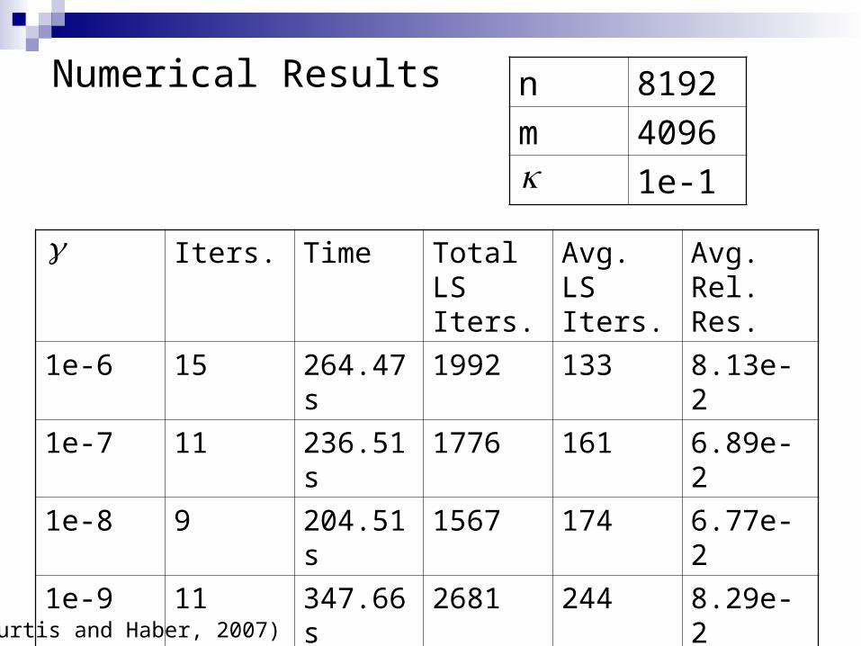
Numerical Results
Iters. Time Total LS Iters.
Avg. LS Iters.
Avg. Rel. Res.
1e-6 15 264.47s 1992 133 8.13e-2
1e-7 11 236.51s 1776 161 6.89e-2
1e-8 9 204.51s 1567 174 6.77e-2
1e-9 11 347.66s 2681 244 8.29e-2
1e-10 16 805.14s 6249 391 8.93e-2
n 8192
m 4096
1e-1
(Curtis and Haber, 2007)
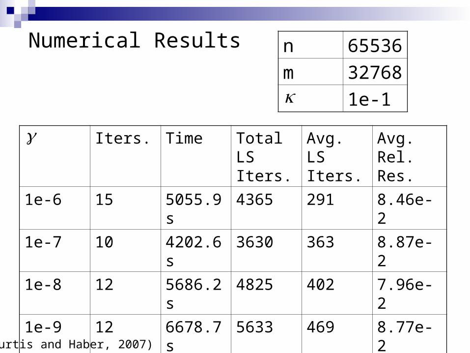
Numerical Results
Iters. Time Total LS Iters.
Avg. LS Iters.
Avg. Rel. Res.
1e-6 15 5055.9s 4365 291 8.46e-2
1e-7 10 4202.6s 3630 363 8.87e-2
1e-8 12 5686.2s 4825 402 7.96e-2
1e-9 12 6678.7s 5633 469 8.77e-2
1e-10 14 14783s 12525 895 8.63e-2
n 65536
m 32768
1e-1
(Curtis and Haber, 2007)
Outline Problem Formulation
Equality constrained optimization Sequential Quadratic Programming
Inexact Framework Unconstrained optimization and nonlinear equations Stopping conditions for linear solver
Global Behavior Merit function and sufficient decrease Satisfying first order conditions
Numerical Results Model inverse problem Accuracy tradeoffs
Final Remarks Future work Negative curvature
Review and Future Challenges Review
Defined a globally convergent inexact SQP algorithm Require only inexact solutions of primal-dual system Require only matrix-vector products involving
objective and constraint function derivatives Results also apply when only reduced Hessian of
Lagrangian is assumed to be positive definite Numerical experience on model problem is promising
Future challenges (Nearly) Singular constraint Jacobians Inexact derivative information Negative curvature etc., etc., etc….
Negative CurvatureBig question
What is the best way to handle negative curvature (i.e., when the reduced Hessian may be indefinite)?
Small question What is the best way to handle negative
curvature in the context of our inexact SQP algorithm?
We have no inertia information! Smaller question
When can we handle negative curvature in the context of our inexact SQP algorithm with NO algorithmic modifications?
When do we know that a given step is OK? Our analysis of the inexact case leads to a few
observations…
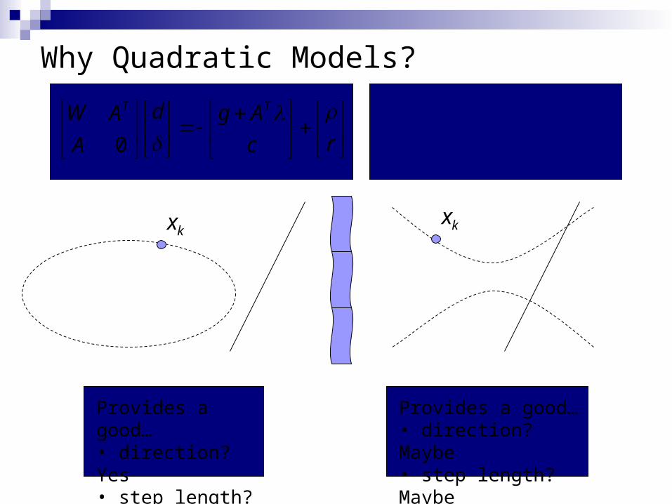
0s.t.
min 21
Adc
Wdddg TT
d
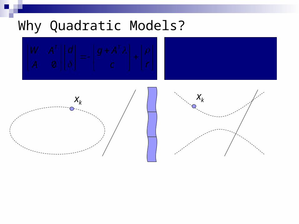
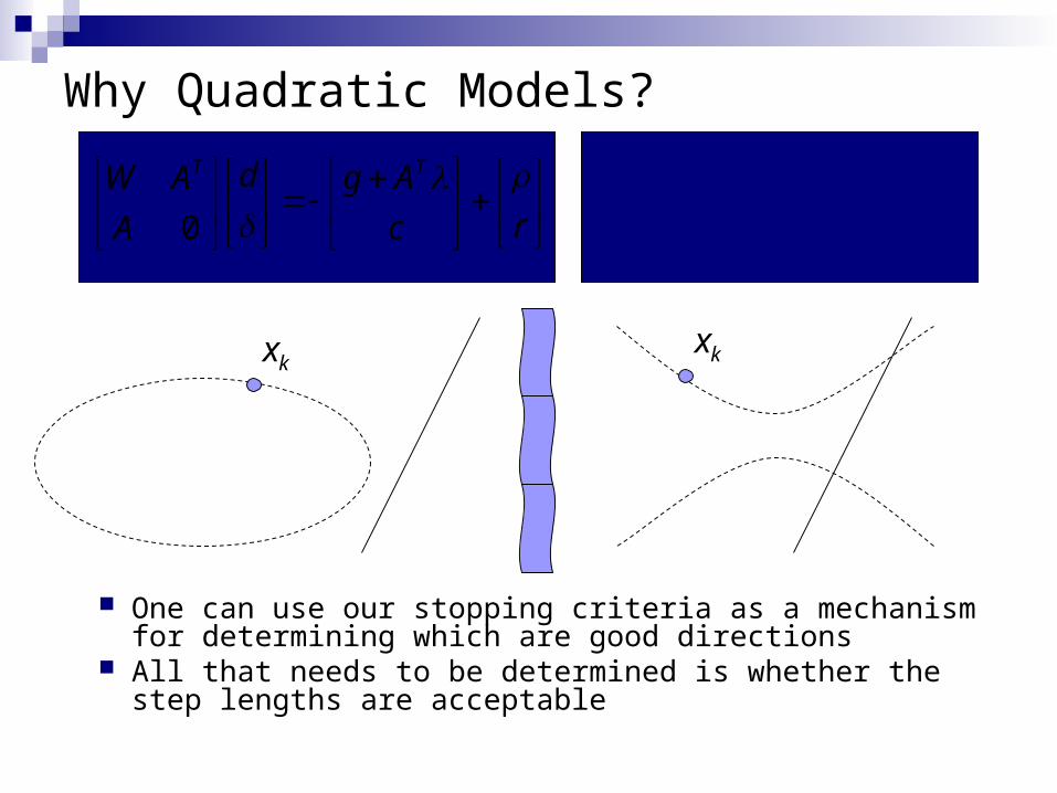
Why Quadratic Models?
rc
Agd
A
AW TT 0
kx kx
0s.t.
min 21
Adc
Wdddg TT
d
Why Quadratic Models?
rc
Agd
A
AW TT 0
kx kx
Provides a good…• direction? Yes• step length? Yes
Provides a good…• direction? Maybe• step length? Maybe
0s.t.
min 21
Adc
Wdddg TT
d
Why Quadratic Models?
rc
Agd
A
AW TT 0
kx kx
One can use our stopping criteria as a mechanism for determining which are good directions
All that needs to be determined is whether the step lengths are acceptable
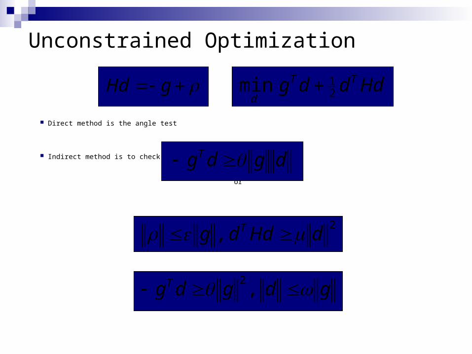
Hdddg TT
d 21 min
Unconstrained Optimization
gHd
Direct method is the angle test
Indirect method is to check the conditions
or
dgdgT
2 , dHddg T
gdgdgT ,2

Hdddg TT
d 21 min
Unconstrained Optimization
gHd
Direct method is the angle test
Indirect method is to check the conditions
or
dgdgT
2 , dHddg T
gdgdgT ,2
step quality step length
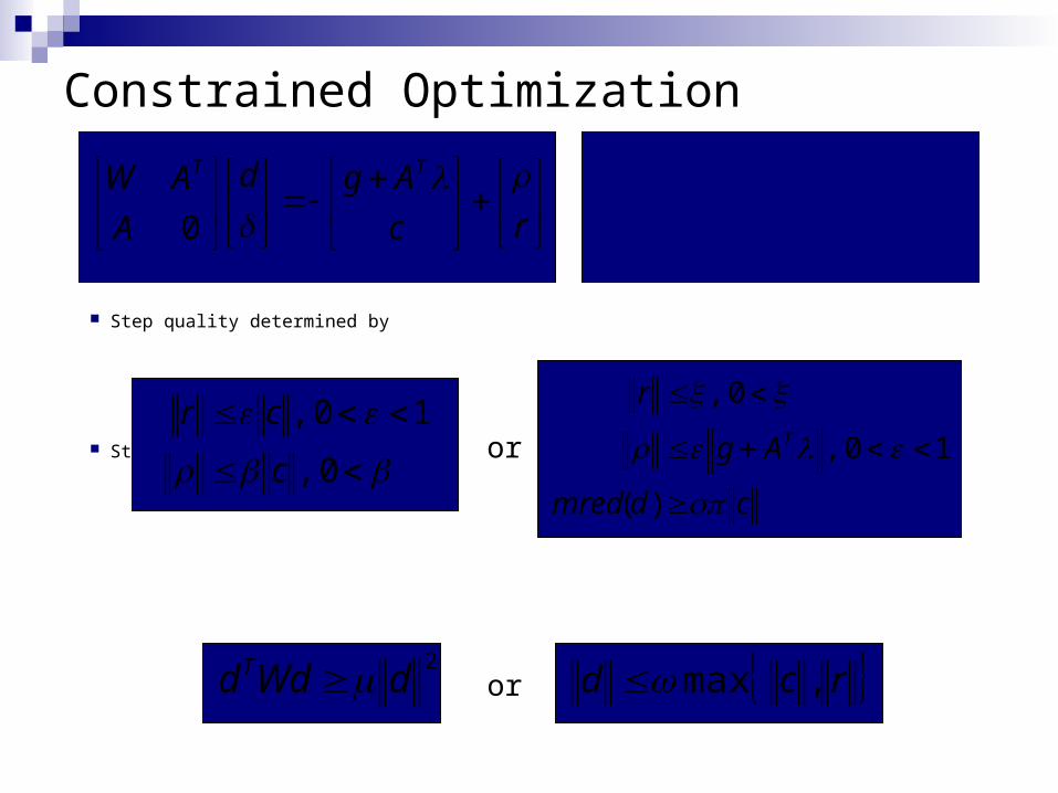
Constrained Optimization
Step quality determined by
Step length determined by
0s.t.
min 21
Adc
Wdddg TT
d
rc
Agd
A
AW TT 0
cdmred
Ag
rT
)(
10 ,
0 ,
0 ,
10 ,
c
cror
rcd , max2dWdd T or

Thanks!
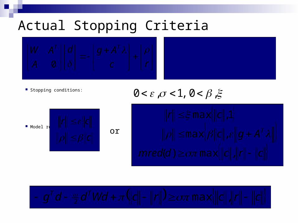
Actual Stopping Criteria
Stopping conditions:
Model reduction condition
0s.t.
min 21
Adc
Wdddg TT
d
rc
Agd
A
AW TT 0
crcdmred
Agc
crT
,max)(
,max
1 ,max
c
cr
or
crcrcWdddg TT ,max2
,0 ,1,0
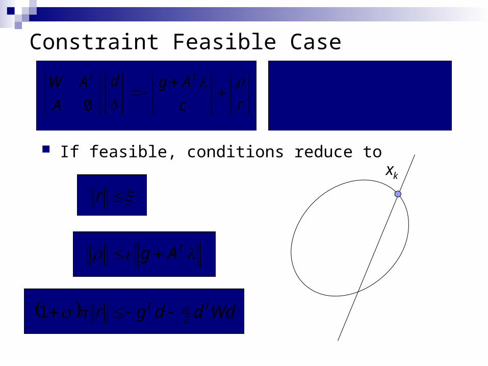
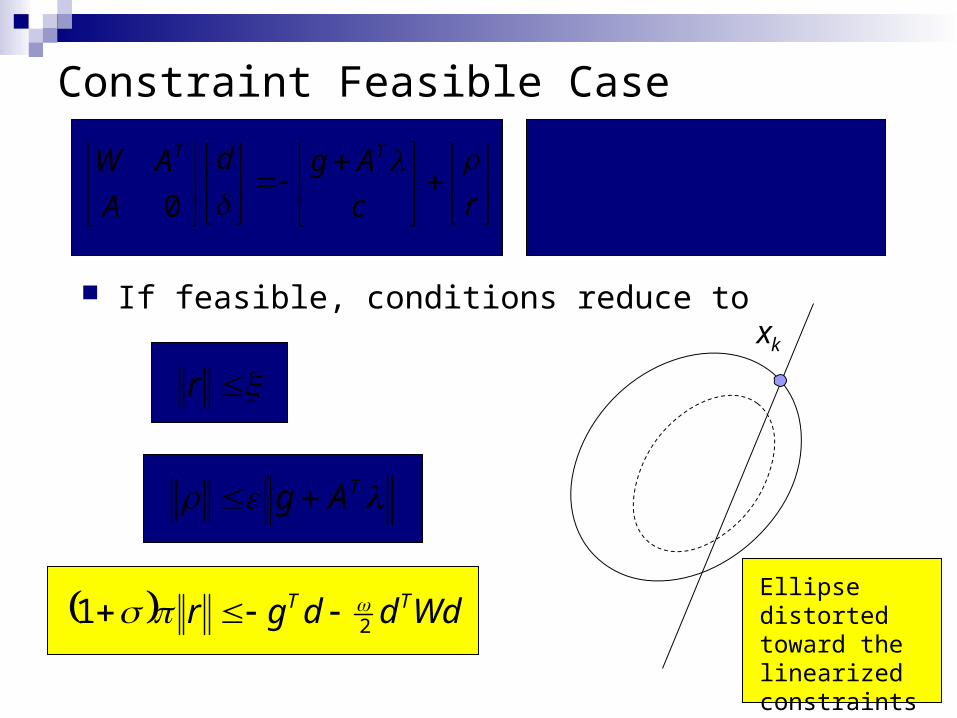
Constraint Feasible Case
If feasible, conditions reduce to
0s.t.
min 21
Adc
Wdddg TT
d
rc
Agd
A
AW TT 0
kx
Wdddgr
Ag
r
TT
T
21
Constraint Feasible Case
If feasible, conditions reduce to
0s.t.
min 21
Adc
Wdddg TT
d
rc
Agd
A
AW TT 0
kx
Wdddgr
Ag
r
TT
T
21
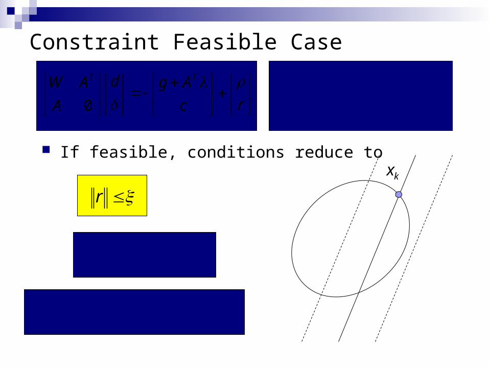
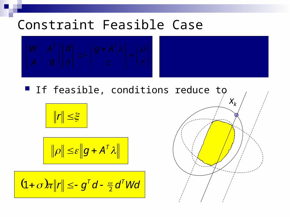
Constraint Feasible Case
If feasible, conditions reduce to
0s.t.
min 21
Adc
Wdddg TT
d
rc
Agd
A
AW TT 0
Wdddgr
Ag
r
TT
T
21
kx
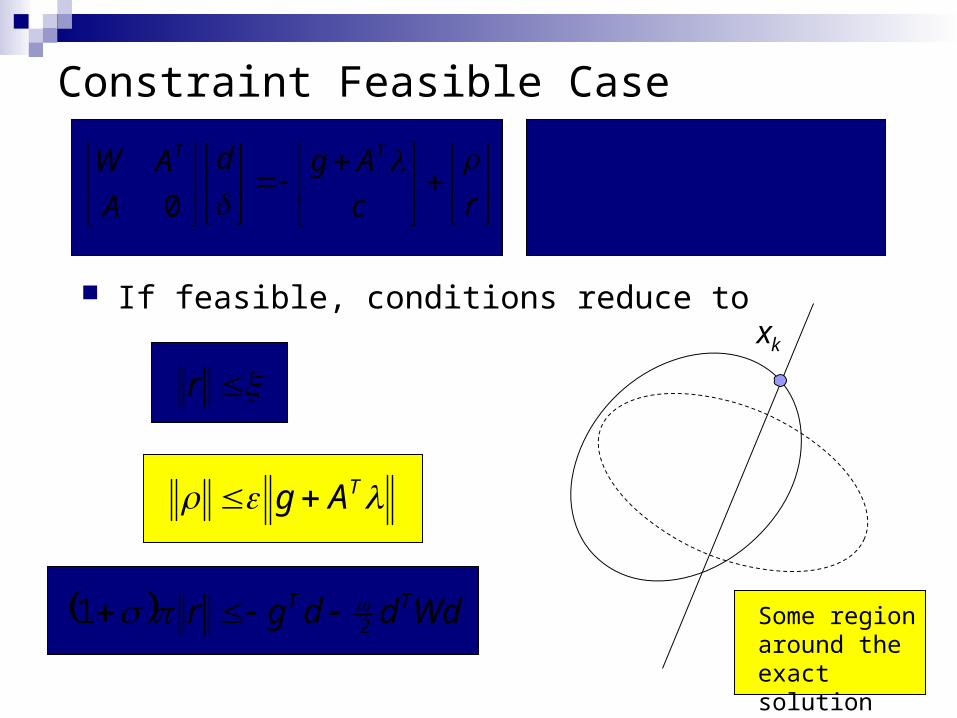
Some region around the exact solution
Constraint Feasible Case
If feasible, conditions reduce to
0s.t.
min 21
Adc
Wdddg TT
d
rc
Agd
A
AW TT 0
kx
Wdddgr
Ag
r
TT
T
21
Ellipse distorted toward the linearized constraints
Constraint Feasible Case
If feasible, conditions reduce to
0s.t.
min 21
Adc
Wdddg TT
d
rc
Agd
A
AW TT 0
Wdddgr
Ag
r
TT
T
21
kx