Franck Nicolleau - Accueil
190
HAL Id: cel-01548212 https://hal.archives-ouvertes.fr/cel-01548212 Submitted on 27 Jun 2017 HAL is a multi-disciplinary open access archive for the deposit and dissemination of sci- entific research documents, whether they are pub- lished or not. The documents may come from teaching and research institutions in France or abroad, or from public or private research centers. L’archive ouverte pluridisciplinaire HAL, est destinée au dépôt et à la diffusion de documents scientifiques de niveau recherche, publiés ou non, émanant des établissements d’enseignement et de recherche français ou étrangers, des laboratoires publics ou privés. Distributed under a Creative Commons Attribution - NonCommercial| 4.0 International License RECIPROCATING ENGINES Franck Nicolleau To cite this version: Franck Nicolleau. RECIPROCATING ENGINES. Master. RECIPROCATING ENGINES, Sheffeld, United Kingdom. 2010, pp.189. cel-01548212
Transcript of Franck Nicolleau - Accueil

HAL Id: cel-01548212https://hal.archives-ouvertes.fr/cel-01548212
Submitted on 27 Jun 2017
HAL is a multi-disciplinary open accessarchive for the deposit and dissemination of sci-entific research documents, whether they are pub-lished or not. The documents may come fromteaching and research institutions in France orabroad, or from public or private research centers.
L’archive ouverte pluridisciplinaire HAL, estdestinée au dépôt et à la diffusion de documentsscientifiques de niveau recherche, publiés ou non,émanant des établissements d’enseignement et derecherche français ou étrangers, des laboratoirespublics ou privés.
Distributed under a Creative Commons Attribution - NonCommercial| 4.0 InternationalLicense
RECIPROCATING ENGINESFranck Nicolleau
To cite this version:Franck Nicolleau. RECIPROCATING ENGINES. Master. RECIPROCATING ENGINES, Sheffield,United Kingdom. 2010, pp.189. cel-01548212

Mechanical Engineering - 14 May 2010 -1-
UNIVERSITY OF SHEFFIELD
Department of Mechanical Engineering
Mappin street, Sheffield, S1 3JD, England
RECIPROCATING ENGINES
Autumn Semester 2010
MEC403 - MEng, semester 7 - MEC6403 - MSc(Res)
Dr. F. C. G. A. Nicolleau
MD54
Telephone: +44 (0)114 22 27700. Direct Line: +44 (0)114 22 27867
Fax: +44 (0)114 22 27890
email: [email protected]
http://www.shef.ac.uk/mecheng/mecheng cms/staff/fcgan/
MEng 4th year Course Tutor : Pr N. Qin
European and Year Abroad Tutor : C. Pinna
MSc(Res) and MPhil Course Director : F. C. G. A. Nicolleau
c© 2010 F C G A Nicolleau, The University of Sheffield

-2- Combustion engines

Table of content -3-
Table of content
Table of content 3
Nomenclature 9
Introduction 13
Acknowledgement 16
I - Introduction and Fundamentals of combustion 171 Introduction to combustion engines 19
1.1 Piston engines . . . . . . . . . . . . . . . . . . . . . . . . . . . . . . . . . . . . . . . . . . . 19
1.2 Other reciprocating engines . . . . . . . . . . . . . . . . . . . . . . . . . . . . . . . . . . . 20
1.2.1 Wankel engine . . . . . . . . . . . . . . . . . . . . . . . . . . . . . . . . . . . . . . 20
1.2.2 HCCI engine . . . . . . . . . . . . . . . . . . . . . . . . . . . . . . . . . . . . . . . 20
1.3 Performance parameters for combustion engines . . . . . . . . . . . . . . . . . . . . . . . . 20
2 Combustion 23
2.1 Stoichiometry . . . . . . . . . . . . . . . . . . . . . . . . . . . . . . . . . . . . . . . . . . . 23
2.1.1 Exercise . . . . . . . . . . . . . . . . . . . . . . . . . . . . . . . . . . . . . . . . . . 23
2.1.2 Products of Combustion . . . . . . . . . . . . . . . . . . . . . . . . . . . . . . . . . 24
2.1.3 Example . . . . . . . . . . . . . . . . . . . . . . . . . . . . . . . . . . . . . . . . . . 24
2.2 Combustion Thermodynamics . . . . . . . . . . . . . . . . . . . . . . . . . . . . . . . . . . 25
2.3 Criteria for equilibrium . . . . . . . . . . . . . . . . . . . . . . . . . . . . . . . . . . . . . 27
2.3.1 Adiabatic closed system (pure substance) . . . . . . . . . . . . . . . . . . . . . . . 27
2.3.2 Isothermal closed system . . . . . . . . . . . . . . . . . . . . . . . . . . . . . . . . 27
2.4 Emissions . . . . . . . . . . . . . . . . . . . . . . . . . . . . . . . . . . . . . . . . . . . . . 28
3 Thermodynamics of reacting gas mixtures 29
3.1 Properties of an ideal gas . . . . . . . . . . . . . . . . . . . . . . . . . . . . . . . . . . . . 29
3.2 Gibbs function changes . . . . . . . . . . . . . . . . . . . . . . . . . . . . . . . . . . . . . . 29
3.3 Analysis of chemical equilibrium . . . . . . . . . . . . . . . . . . . . . . . . . . . . . . . . 30
3.4 Example . . . . . . . . . . . . . . . . . . . . . . . . . . . . . . . . . . . . . . . . . . . . . . 31
3.5 More realistic reactions in engines . . . . . . . . . . . . . . . . . . . . . . . . . . . . . . . 34
3.5.1 Neglecting NO (f = 0) . . . . . . . . . . . . . . . . . . . . . . . . . . . . . . . . . . 34
3.5.2 With NO concentrations . . . . . . . . . . . . . . . . . . . . . . . . . . . . . . . . . 35
3.5.3 Exercise . . . . . . . . . . . . . . . . . . . . . . . . . . . . . . . . . . . . . . . . . . 35
3.5.4 Exercise . . . . . . . . . . . . . . . . . . . . . . . . . . . . . . . . . . . . . . . . . . 35
3.5.5 Exercise . . . . . . . . . . . . . . . . . . . . . . . . . . . . . . . . . . . . . . . . . . 36
3.5.6 Exercise . . . . . . . . . . . . . . . . . . . . . . . . . . . . . . . . . . . . . . . . . . 36
3.6 Kinetics . . . . . . . . . . . . . . . . . . . . . . . . . . . . . . . . . . . . . . . . . . . . . . 36

-4- Table of content
4 Simple physics of flames and combustion 37
4.1 Premixed laminar flame . . . . . . . . . . . . . . . . . . . . . . . . . . . . . . . . . . . . . 37
4.2 Diffusion flame . . . . . . . . . . . . . . . . . . . . . . . . . . . . . . . . . . . . . . . . . . 38
4.3 Detonation Wave . . . . . . . . . . . . . . . . . . . . . . . . . . . . . . . . . . . . . . . . . 39
4.4 Ignition in Piston Engine . . . . . . . . . . . . . . . . . . . . . . . . . . . . . . . . . . . . 39
4.5 Turbulent flame . . . . . . . . . . . . . . . . . . . . . . . . . . . . . . . . . . . . . . . . . . 39
4.5.1 Turbulence parameters . . . . . . . . . . . . . . . . . . . . . . . . . . . . . . . . . . 39
4.5.2 Mixing . . . . . . . . . . . . . . . . . . . . . . . . . . . . . . . . . . . . . . . . . . . 39
4.5.3 Turbulent flame front . . . . . . . . . . . . . . . . . . . . . . . . . . . . . . . . . . 40
4.6 Flame Quench . . . . . . . . . . . . . . . . . . . . . . . . . . . . . . . . . . . . . . . . . . 42
4.7 Diesel combustion . . . . . . . . . . . . . . . . . . . . . . . . . . . . . . . . . . . . . . . . 43
Appendix of chapter 4 . . . . . . . . . . . . . . . . . . . . . . . . . . . . . . . . . . . . . . . . . 44
4.A Bunsen burner . . . . . . . . . . . . . . . . . . . . . . . . . . . . . . . . . . . . . . 44
4.B Turbulent flame propagation . . . . . . . . . . . . . . . . . . . . . . . . . . . . . . 44
4.C Role of the Swirl . . . . . . . . . . . . . . . . . . . . . . . . . . . . . . . . . . . . 44
5 Equations for reactive flows 45
5.1 Mass conservation of a passive scalar . . . . . . . . . . . . . . . . . . . . . . . . . . . . . . 45
5.1.1 Mass variation inside a control volume . . . . . . . . . . . . . . . . . . . . . . . . . 45
5.1.2 The notion of flux . . . . . . . . . . . . . . . . . . . . . . . . . . . . . . . . . . . . 46
5.1.3 The divergence theorem . . . . . . . . . . . . . . . . . . . . . . . . . . . . . . . . . 47
5.1.4 The continuity equation . . . . . . . . . . . . . . . . . . . . . . . . . . . . . . . . . 48
5.2 Un-reactive mixture . . . . . . . . . . . . . . . . . . . . . . . . . . . . . . . . . . . . . . . 49
5.2.1 The scalar equation . . . . . . . . . . . . . . . . . . . . . . . . . . . . . . . . . . . 49
5.2.2 Mass diffusion . . . . . . . . . . . . . . . . . . . . . . . . . . . . . . . . . . . . . . 50
5.2.3 The Fick law . . . . . . . . . . . . . . . . . . . . . . . . . . . . . . . . . . . . . . . 51
5.2.4 Exercise . . . . . . . . . . . . . . . . . . . . . . . . . . . . . . . . . . . . . . . . . . 53
5.2.5 Exercise . . . . . . . . . . . . . . . . . . . . . . . . . . . . . . . . . . . . . . . . . . 53
5.2.6 Exercise . . . . . . . . . . . . . . . . . . . . . . . . . . . . . . . . . . . . . . . . . . 53
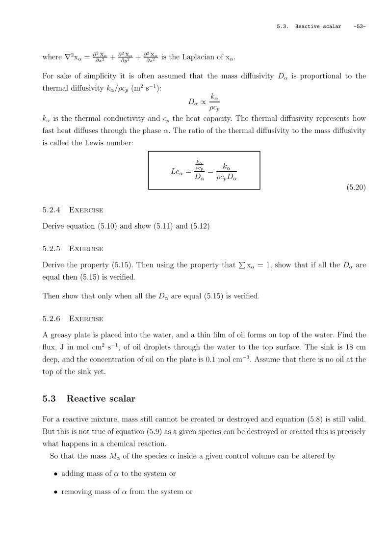
5.3 Reactive scalar . . . . . . . . . . . . . . . . . . . . . . . . . . . . . . . . . . . . . . . . . . 53
5.4 The energy conservation . . . . . . . . . . . . . . . . . . . . . . . . . . . . . . . . . . . . . 54
5.4.1 Adding heat and work . . . . . . . . . . . . . . . . . . . . . . . . . . . . . . . . . . 55
5.4.2 Volume force . . . . . . . . . . . . . . . . . . . . . . . . . . . . . . . . . . . . . . . 57
5.4.3 Heat production . . . . . . . . . . . . . . . . . . . . . . . . . . . . . . . . . . . . . 58
5.4.4 The energy balance . . . . . . . . . . . . . . . . . . . . . . . . . . . . . . . . . . . . 58
5.4.5 Enthalpy conservation . . . . . . . . . . . . . . . . . . . . . . . . . . . . . . . . . . 59
5.4.6 Total enthalpy . . . . . . . . . . . . . . . . . . . . . . . . . . . . . . . . . . . . . . 59
5.4.7 Exercise . . . . . . . . . . . . . . . . . . . . . . . . . . . . . . . . . . . . . . . . . . 59
5.5 Energy equation for a reacting mixture . . . . . . . . . . . . . . . . . . . . . . . . . . . . . 60

Table of content -5-
5.5.1 Exercise . . . . . . . . . . . . . . . . . . . . . . . . . . . . . . . . . . . . . . . . . . 60
5.5.2 Energy conservation for a mixture . . . . . . . . . . . . . . . . . . . . . . . . . . . 60
5.5.3 Exercise . . . . . . . . . . . . . . . . . . . . . . . . . . . . . . . . . . . . . . . . . . 62
5.6 Enthalpy conservation for a reactive mixture . . . . . . . . . . . . . . . . . . . . . . . . . 62
5.6.1 Exercise . . . . . . . . . . . . . . . . . . . . . . . . . . . . . . . . . . . . . . . . . . 62
5.7 Heat transfer . . . . . . . . . . . . . . . . . . . . . . . . . . . . . . . . . . . . . . . . . . . 62
5.7.1 Heat transfer through mass transfer . . . . . . . . . . . . . . . . . . . . . . . . . . 62
5.7.2 Modelling of the total Heat transfer . . . . . . . . . . . . . . . . . . . . . . . . . . 63
5.8 Momentum equation . . . . . . . . . . . . . . . . . . . . . . . . . . . . . . . . . . . . . . . 65
Revision questionnaire of Part I 67
II - Piston engines 696 Piston engines 71
6.1 Performance Parameters for Piston Engines . . . . . . . . . . . . . . . . . . . . . . . . . . 71
6.1.1 Swept volume . . . . . . . . . . . . . . . . . . . . . . . . . . . . . . . . . . . . . . . 71
6.1.2 Torque . . . . . . . . . . . . . . . . . . . . . . . . . . . . . . . . . . . . . . . . . . . 71
6.1.3 Power . . . . . . . . . . . . . . . . . . . . . . . . . . . . . . . . . . . . . . . . . . . 71
6.1.4 Volumetric efficiency, ηvol . . . . . . . . . . . . . . . . . . . . . . . . . . . . . . . . 72
6.2 Mean effective pressure . . . . . . . . . . . . . . . . . . . . . . . . . . . . . . . . . . . . . . 72
6.2.1 Brake mean effective pressure pm . . . . . . . . . . . . . . . . . . . . . . . . . . . . 72
6.2.2 Indicated mean effective pressure pmi . . . . . . . . . . . . . . . . . . . . . . . . . 74
6.2.3 Mechanical efficiency . . . . . . . . . . . . . . . . . . . . . . . . . . . . . . . . . . . 74
6.3 Exercise . . . . . . . . . . . . . . . . . . . . . . . . . . . . . . . . . . . . . . . . . . . . . . 74
Appendix of chapter 6 . . . . . . . . . . . . . . . . . . . . . . . . . . . . . . . . . . . . . . . . . 76
6.A Piston engine survey . . . . . . . . . . . . . . . . . . . . . . . . . . . . . . . . . . 76
7 Spark ignition engines 77
7.1 Ideal Otto cycle (Beau de Rochas) . . . . . . . . . . . . . . . . . . . . . . . . . . . . . . . 77
7.1.1 Exercise . . . . . . . . . . . . . . . . . . . . . . . . . . . . . . . . . . . . . . . . . . 79
7.2 Realistic thermodynamic cycles . . . . . . . . . . . . . . . . . . . . . . . . . . . . . . . . . 79
7.2.1 Effects of fuel-air Otto cycle . . . . . . . . . . . . . . . . . . . . . . . . . . . . . . . 79
7.2.2 Effects of departure from constant volume . . . . . . . . . . . . . . . . . . . . . . . 79
7.2.3 Effects of Heat losses from cylinder walls . . . . . . . . . . . . . . . . . . . . . . . . 80
7.2.4 Comparison with engine measurements . . . . . . . . . . . . . . . . . . . . . . . . . 80
7.3 Combustion in spark ignition engines . . . . . . . . . . . . . . . . . . . . . . . . . . . . . . 80
7.3.1 The ’normal’ combustion sequence . . . . . . . . . . . . . . . . . . . . . . . . . . . 80
7.3.2 Effect of fuel/air ratio on ignition limits . . . . . . . . . . . . . . . . . . . . . . . . 81
7.4 Knock in Spark ignition Engines (’Spark Knock’, ’Pinking’, ’Detonation’) . . . . . . . . . 81
7.4.1 The phenomenon . . . . . . . . . . . . . . . . . . . . . . . . . . . . . . . . . . . . . 81
7.4.2 The effects . . . . . . . . . . . . . . . . . . . . . . . . . . . . . . . . . . . . . . . . 82

-6- Table of content
7.4.3 Prevention of knock . . . . . . . . . . . . . . . . . . . . . . . . . . . . . . . . . . . 82
7.4.4 Octane Number . . . . . . . . . . . . . . . . . . . . . . . . . . . . . . . . . . . . . . 82
Appendix of chapter 7 . . . . . . . . . . . . . . . . . . . . . . . . . . . . . . . . . . . . . . . . . 84
7.A Ideal cycle /real cycle comparison . . . . . . . . . . . . . . . . . . . . . . . . . . . 84
8 Spark ignition engines: combustion control 85
8.1 Throttle control . . . . . . . . . . . . . . . . . . . . . . . . . . . . . . . . . . . . . . . . . . 85
8.2 Fuel Supply . . . . . . . . . . . . . . . . . . . . . . . . . . . . . . . . . . . . . . . . . . . . 85
8.2.1 Carburettor . . . . . . . . . . . . . . . . . . . . . . . . . . . . . . . . . . . . . . . . 85
8.2.2 Injection system . . . . . . . . . . . . . . . . . . . . . . . . . . . . . . . . . . . . . 87
8.2.3 Multi point injection (MPI) . . . . . . . . . . . . . . . . . . . . . . . . . . . . . . . 87
8.3 Performance . . . . . . . . . . . . . . . . . . . . . . . . . . . . . . . . . . . . . . . . . . . . 87
8.4 Combustion chamber design . . . . . . . . . . . . . . . . . . . . . . . . . . . . . . . . . . . 88
8.5 Emissions . . . . . . . . . . . . . . . . . . . . . . . . . . . . . . . . . . . . . . . . . . . . . 89
8.5.1 Combustion Kinetics . . . . . . . . . . . . . . . . . . . . . . . . . . . . . . . . . . . 89
8.5.2 Hydrocarbons (see Heywood Fig. 11-1) . . . . . . . . . . . . . . . . . . . . . . . . . 89
8.5.3 Pollution of the Environment . . . . . . . . . . . . . . . . . . . . . . . . . . . . . . 90
8.5.4 Emissions control . . . . . . . . . . . . . . . . . . . . . . . . . . . . . . . . . . . . . 90
8.6 Stratified charge . . . . . . . . . . . . . . . . . . . . . . . . . . . . . . . . . . . . . . . . . 90
8.7 Gas exchange processes . . . . . . . . . . . . . . . . . . . . . . . . . . . . . . . . . . . . . 91
8.7.1 Sequence of events in four stroke cycle engines . . . . . . . . . . . . . . . . . . . . 92
8.8 Admission Valve . . . . . . . . . . . . . . . . . . . . . . . . . . . . . . . . . . . . . . . . . 92
8.8.1 Exercise . . . . . . . . . . . . . . . . . . . . . . . . . . . . . . . . . . . . . . . . . . 93
Appendix of chapter 8 . . . . . . . . . . . . . . . . . . . . . . . . . . . . . . . . . . . . . . . . . 94
8.A Diagram of an L-Jetronic system . . . . . . . . . . . . . . . . . . . . . . . . . . . 94
8.B European Vehicle Exhaust Emission Standards . . . . . . . . . . . . . . . . . . . 95
9 Combustion ignition engines: diesel engines 97
9.1 Combustion . . . . . . . . . . . . . . . . . . . . . . . . . . . . . . . . . . . . . . . . . . . . 97
9.1.1 Fundamental features . . . . . . . . . . . . . . . . . . . . . . . . . . . . . . . . . . 97
9.1.2 Requirements . . . . . . . . . . . . . . . . . . . . . . . . . . . . . . . . . . . . . . . 98
9.1.3 Combustion sequence . . . . . . . . . . . . . . . . . . . . . . . . . . . . . . . . . . 98
9.2 Design aspects . . . . . . . . . . . . . . . . . . . . . . . . . . . . . . . . . . . . . . . . . . 98
9.2.1 Fuel and air requirements . . . . . . . . . . . . . . . . . . . . . . . . . . . . . . . . 98
9.2.2 General . . . . . . . . . . . . . . . . . . . . . . . . . . . . . . . . . . . . . . . . . . 99
9.2.3 Fuel Injection Systems . . . . . . . . . . . . . . . . . . . . . . . . . . . . . . . . . . 99
9.3 Fuel and cetane number . . . . . . . . . . . . . . . . . . . . . . . . . . . . . . . . . . . . . 100
9.4 Emissions . . . . . . . . . . . . . . . . . . . . . . . . . . . . . . . . . . . . . . . . . . . . . 100
9.4.1 Incomplete combustion products . . . . . . . . . . . . . . . . . . . . . . . . . . . . 100
9.4.2 NOx production . . . . . . . . . . . . . . . . . . . . . . . . . . . . . . . . . . . . . 101

Table of content -7-
9.5 Spark ignition engines compared to compression ignition engines . . . . . . . . . . . . . . 101
9.5.1 Emissions . . . . . . . . . . . . . . . . . . . . . . . . . . . . . . . . . . . . . . . . . 101
9.5.2 Naturally Aspirated Engines: effect of overall fuel/air ratio . . . . . . . . . . . . . 101
9.5.3 Typical parameters . . . . . . . . . . . . . . . . . . . . . . . . . . . . . . . . . . . . 102
9.5.4 Fuel consumption . . . . . . . . . . . . . . . . . . . . . . . . . . . . . . . . . . . . . 102
10 Two stroke cycle engines 103
10.1 Sequence of events . . . . . . . . . . . . . . . . . . . . . . . . . . . . . . . . . . . . . . . . 103
10.2 Design Options . . . . . . . . . . . . . . . . . . . . . . . . . . . . . . . . . . . . . . . . . . 104
10.3 Scavenge process . . . . . . . . . . . . . . . . . . . . . . . . . . . . . . . . . . . . . . . . . 104
10.3.1 Dimensionless performance parameters . . . . . . . . . . . . . . . . . . . . . . . . . 104
10.3.2 Perfect displacement model . . . . . . . . . . . . . . . . . . . . . . . . . . . . . . . 105
10.3.3 Complete mixing . . . . . . . . . . . . . . . . . . . . . . . . . . . . . . . . . . . . . 106
10.3.4 Short Circuit Flow . . . . . . . . . . . . . . . . . . . . . . . . . . . . . . . . . . . . 107
10.3.5 Combined Scavenge Model . . . . . . . . . . . . . . . . . . . . . . . . . . . . . . . 107
10.3.6 Exercise . . . . . . . . . . . . . . . . . . . . . . . . . . . . . . . . . . . . . . . . . . 108
10.4 Power losses from scavenge flows . . . . . . . . . . . . . . . . . . . . . . . . . . . . . . . . 108
10.4.1 Exercise . . . . . . . . . . . . . . . . . . . . . . . . . . . . . . . . . . . . . . . . . . 109
10.5 Comparison with four stroke engines . . . . . . . . . . . . . . . . . . . . . . . . . . . . . . 109
Revision questionnaire of Part II 111
III - Supercharging and Turbocharging 11311 Supercharging and turbocharging 115
11.1 Purpose . . . . . . . . . . . . . . . . . . . . . . . . . . . . . . . . . . . . . . . . . . . . . . 115
11.1.1 supercharger . . . . . . . . . . . . . . . . . . . . . . . . . . . . . . . . . . . . . . . 115
11.1.2 Turbochargers . . . . . . . . . . . . . . . . . . . . . . . . . . . . . . . . . . . . . . 116
11.1.3 Other devices . . . . . . . . . . . . . . . . . . . . . . . . . . . . . . . . . . . . . . . 117
11.2 Thermodynamic analysis of turbochargers . . . . . . . . . . . . . . . . . . . . . . . . . . . 117
11.3 Constant pressure turbocharging . . . . . . . . . . . . . . . . . . . . . . . . . . . . . . . . 119
11.4 Pulse system . . . . . . . . . . . . . . . . . . . . . . . . . . . . . . . . . . . . . . . . . . . 119
11.5 Energy available . . . . . . . . . . . . . . . . . . . . . . . . . . . . . . . . . . . . . . . . . 121
11.5.1 Expansion energy available at exhaust release point . . . . . . . . . . . . . . . . . 122
11.5.2 Energy available from an adiabatic exhaust turbine: ideal pulse turbine . . . . . . 123
11.5.3 Energy available from an adiabatic exhaust turbine: Constant pressure exhaust
manifold (4 stroke) . . . . . . . . . . . . . . . . . . . . . . . . . . . . . . . . . . . . 124
12 Turbocharging design and modelling 127
12.1 Design analysis . . . . . . . . . . . . . . . . . . . . . . . . . . . . . . . . . . . . . . . . . . 127
12.2 Turbocharger power balance . . . . . . . . . . . . . . . . . . . . . . . . . . . . . . . . . . . 127
12.3 Mean Temperature Te from known cylinder release conditions . . . . . . . . . . . . . . . . 129
12.4 Empirical relationship for Te . . . . . . . . . . . . . . . . . . . . . . . . . . . . . . . . . . 129

-8- Table of content
12.5 Example for a good diesel . . . . . . . . . . . . . . . . . . . . . . . . . . . . . . . . . . . . 130
12.6 Exercise . . . . . . . . . . . . . . . . . . . . . . . . . . . . . . . . . . . . . . . . . . . . . . 131
12.7 Exercise . . . . . . . . . . . . . . . . . . . . . . . . . . . . . . . . . . . . . . . . . . . . . . 131
13 Elements of turbomachinery 133
13.1 Dimensional analysis of compressible flows through turbomachines . . . . . . . . . . . . . 133
13.2 Velocity limits in a compressor . . . . . . . . . . . . . . . . . . . . . . . . . . . . . . . . . 134
13.3 Compressor characteristic . . . . . . . . . . . . . . . . . . . . . . . . . . . . . . . . . . . . 134
13.3.1 Surge . . . . . . . . . . . . . . . . . . . . . . . . . . . . . . . . . . . . . . . . . . . 136
13.3.2 Stall . . . . . . . . . . . . . . . . . . . . . . . . . . . . . . . . . . . . . . . . . . . . 136
13.3.3 Compressor choice . . . . . . . . . . . . . . . . . . . . . . . . . . . . . . . . . . . . 136
13.4 Real effects in exhaust turbine Systems . . . . . . . . . . . . . . . . . . . . . . . . . . . . 137
Revision questionnaire of Part III 139
IV - Other reciprocating engines 14114 Rotary Engine (Wankel Engine) 143
15 HCCI Engine 145
Revision questionnaire of Part IV 147
Conclusion 149
List of Figures 151
MEC403 Data sheets 155
Course Work 159
Solutions to exercises 161
References 187

Nomenclature -9-
Nomenclature
Units refer to international system and are the one usually used in the course
B : bore of the cylinder (m)
bmep : brake mean effective pressure
bsfc : break specific fuel consumption (kg.J−1 but usually in kg.kWh−1)
cp : specific heat for enthalpy (J.K−1.kg−1)
cv : specific heat for energy (J.K−1.kg−1)
f : fuel/air (mass) ratio
g : specific Gibbs function (J.kg−1)
h : specific enthalpy (J.kg−1)
h : molar enthalpy (J.mol−1)
isfc : indicated specific fuel consumption (kg.J−1 but usually in kg.kWh−1)
m : mass (kg)
m : molar mass (kg.mol−1)
n : number of moles of gas (mol)
ncy : number of cylinders
p : pressure (Pa i.e. kg.m−1.s−2)
pbm : brake mean effective pressure (Pa)
pfm : friction mean effective pressure (Pa)
pm : mean effective pressure (Pa)
pmi : indicated mean effective pressure (Pa)
q : heat per unit mass (J.kg−1)
R : (or Ru) molar gas constant (universal) 8.3145 J.mol−1.K−1

-10- Nomenclature
R : gas constant Rm (J.kg−1.K−1)
rp : pressure ratio in gas turbine cycle
rv : compression ratio
s : specific entropy (J.K−1.kg−1)
sfc : specific fuel consumption (kg.J−1 but usually in kg.kWh−1)
s : molar entropy (J.K−1.mol−1)
T : Temperature (K or C)
u : specific internal energy (J.kg−1)
U : internal energy
V : volume (m3)
Vs : swept volume (m3)
v : molar volume Vn (m3.mol−1)
V : velocity
w : work per unit mass (J.kg−1)
Greek symbols
α : air/fuel mass ratio
αv : air/fuel volume ratio
γ : ratio of heat capacity γ =cp
cv=
cp
cv
φ : equivalence ratio
ηo : overall efficiency
ηvol : volumetric efficiency
ηc : compressor efficiency
ηt : turbine efficiency
λ : excess air ratio
ρ : density 1v = m
V (kg.m−3)

Nomenclature -11-
τ : crankshaft torque (N.m)
Abbreviation
EGR : exhaust gas recirculation
EVC : Exhaust valve closes
IVC : inlet valve closes
IVO : inlet valve opens
LCV : low calorific value
PF : pulse factor
PLF : pressure loss factor
WOT : wide opened throttle
Notation
˜ : molar, quantity A = A per moles
specific : quantity per unit mass, usually small letters

-12- Nomenclature

Introduction -13-
Introduction
Purpose
This module is largely (but freely) inspired from a previous one delivered by Mr R. Saunders
(MPE310 Combustion Engines). It relies on thermodynamics basics acquired in 1st (Beck, 2000)
and 2nd (Smyth, 1999) year of M.Eng. in Mechanical Engineering. Elements of the course MEC310
(Nicolleau, 2001) may be useful.
This module considers the performance of and emissions from reciprocating combustion engines.
It should enable students to recognise the salient aspects of combustion thermodynamics and
flame structure in each type of engine and to perform simple chemical equilibrium analyses; to
analyse the performance and explain the emissions characteristics of piston engines, including
spark ignition, compression ignition and turbocharging.
In Practice
• 12 weeks of teaching,
• 20 off one-hour formal lectures,
• 4 hours used as class example, applications, class revision,
• 2-hour seminar given by Pr G. Kalghatgi
• a two-hour examination.
Lectures in 2006:SG-ME04: Tuesday 09:00-09:50
SG-F110: Friday 11:10-12:00

-14- Introduction
Lecture List (indicative)
Week 1 26 09 2010 Lecture 1 introduction, chapter 1, chapter 2
29 09 2010 Lecture 2 chapter 2, chapter 3
Week 2 03 10 2010 Lecture 3 chapter 3
06 10 2010 Lecture 4 chapter 3
Week 3 10 10 2010 Lecture 5 chapter 4
13 10 2010 Lecture 6 chapter 5 - Scalar transport equation
Week 4 17 10 2010 Lecture 7 chapter 5 - enthalpy of a reactive mixture
20 10 2010 Lecture 8 chapter 5, chapter 6
Week 5 24 10 2010 Lecture 9 chapter 6, chapter 7
27 10 2010 Lecture 10 chapter 7, chapter 8
Week 6 31 10 2010 Lecture 11 chapter 8, chapter 9
03 11 2010 Lecture 12 chapter 9
Week 7 07 11 2010 Lecture 13 chapter 9, chapter 10
10 11 2010 Lecture 14 NO LECTURE account for tutorial
Week 8 14 11 2010 Lecture 15 chapter 10, chapter 11
17 11 2010 Lecture 16 chapter 12
Week 9 21 11 2010 Lecture 17 chapter 13
24 11 2010 Lecture 18 chapter 14 - Wankel engine
Week 10 28 11 2010 Lecture 19 chapter 15 - HCCI engine - Last lecture
01 12 2010 Lecture 20 NO LECTURE account for tutorial
Week 11 05 12 2010 Lecture 21 NO LECTURE account for tutorial
08 12 2010 Lecture 22 NO LECTURE account for tutorial
Week 12 12 12 2010 Lecture 23 NO LECTURE, replaced by a seminar TBA
15 12 2010 Lecture 24 NO LECTURE, replaced by a seminar TBA
Seminar Week 7 ????
Week 13 - 15 15 01 2007 to 03 02 2007 EXAMINATIONS
The Course is now housed on the WebCT of the university of Sheffield
http://vista.shef.ac.uk (formally http://webct.shef.ac.uk)
Contact me if you have difficulty accessing the site.

Introduction -15-
Examination
A two hour formal examination 80 %
- a series of questions on the course 30 %
- 2 exercises (25 % each) 50 %
One course work 20 % - a report on the 2-hour seminar
Recommended Textbooks
Tables required:
The Little book of thermodynamics
You can find it on WebCT or buy a copy 1
Recommended Textbooks
Stone (1999), Heywood (1988)

-16- Acknowledgement
Acknowledgement
I gratefully acknowledge help and advice from Mr R. Saunders Lecturer in the Department of
Mechanical Engineering, The University of Sheffield.
Prof. G. T. Kalghatgi - Senior Scientist, Shell Global Solutions (UK) - participation to the Com-
bustion chapter when he was a Visiting Professor in the Department of Mechanical Engineering
was greatly appreciated.
Prof. X. Lys, former Senior Scientist Renault (France) and visiting professor at Ecole Centrale de
Lyon was kind enough to give helpful comments on the Piston Engine part.

part I: Introduction and Fundamentals of combustion -17-
Part I
Introduction and Fundamentals of
combustion

-18- part I: Introduction and Fundamentals of combustion

Chapter 1. Introduction to combustion engines -19-
Chapter 1: Introduction to combustion engines
There are two main combustion engines
• Piston engines either spark ignition or diesel
• and gas turbine
1.1 Piston engines
• Four stroke engine Four and two stroke engines can be either spark engine or diesel engine
from Heywood (1988)figure 1-2 page 10
Figure 1.1. The four stroke operating cycle
In a spark engineair and fuel are premixed before the compressionand the combustion needs to be initiated with a spark
In a compression engine (diesel)fuel is sprayed into the compressed airand the resulting compressed mixture auto-ignites locally.
Figure 1.2. Four stroke piston engine

-20- Chapter 1. Introduction to combustion engines
• Two stroke spark engine
Figure 1.3. Two stroke piston engine
1.2 Other reciprocating engines
1.2.1 Wankel engine
1.2.2 HCCI engine
1.3 Performance parameters for combustion engines
Environment at T0 , P0
COMBUSTION
(Q0)
(1) (2)
W
REACTANTS PRODUCTS
POWER
OUTPUT
Figure 1.4. Thermal efficiency
Thermal Efficiency ηth also known as fuel conversion efficiency ηf : (overall arbitrary efficiency
ηo Nicolleau (2001))
ηth =power output
fuel energy input rate=
W
mf × LCV
(1.1)

1.3. Performance parameters for combustion engines -21-
where
mf is the fuel mass flow rate
LCV is the Lower Calorific Value of fuel
(i.e. combustion ∆h per kg of fuel when H2O in products is not condensed)
specific fuel consumption
sfc =mf
W(1.2)
It is usually given in kg.kWh−1:
sfc = 3600 × mf
W=
3600
ηthLCVin kg.kWh−1 (1.3)
(in formula (1.3) has to be in kJ.kg−1.) For piston engines (see chapter 6) this can be either a
brake measurement bsfc or based on indicated power isfc.
Air/fuel (mass) ratio:
α =air mass
fuel mass=
1
f(1.4)
where f is the fuel/air ratio. Also
αv =air volume
fuel volume=
moles of air
moles of fuel
(e.g. natural gas.)

-22- Chapter 1. Introduction to combustion engines
Chapter 2. Combustion -23-
Chapter 2: Combustion
2.1 Stoichiometry
Fuel is normally a hydrocarbon (CxHy) air is the oxidant (approximatively 21 % of oxygen O2, 79
% of nitrogen N2 by volume or mol)
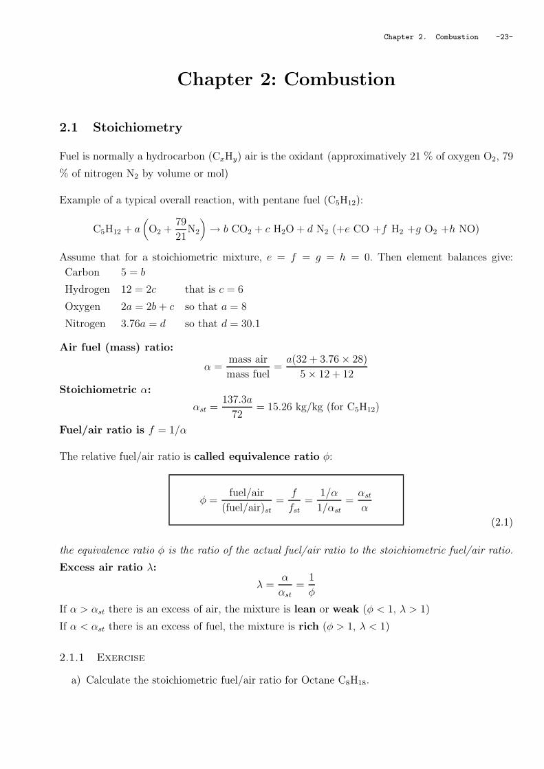
Example of a typical overall reaction, with pentane fuel (C5H12):
C5H12 + a(O2 +
79
21N2
)→ b CO2 + c H2O + d N2 (+e CO +f H2 +g O2 +h NO)
Assume that for a stoichiometric mixture, e = f = g = h = 0. Then element balances give:
Carbon 5 = b
Hydrogen 12 = 2c that is c = 6
Oxygen 2a = 2b + c so that a = 8
Nitrogen 3.76a = d so that d = 30.1
Air fuel (mass) ratio:
α =mass air
mass fuel=
a(32 + 3.76 × 28)
5 × 12 + 12
Stoichiometric α:
αst =137.3a
72= 15.26 kg/kg (for C5H12)
Fuel/air ratio is f = 1/α
The relative fuel/air ratio is called equivalence ratio φ:
φ =fuel/air
(fuel/air)st
=f
fst
=1/α
1/αst
=αst
α
(2.1)
the equivalence ratio φ is the ratio of the actual fuel/air ratio to the stoichiometric fuel/air ratio.
Excess air ratio λ:
λ =α
αst=
1
φ
If α > αst there is an excess of air, the mixture is lean or weak (φ < 1, λ > 1)
If α < αst there is an excess of fuel, the mixture is rich (φ > 1, λ < 1)
2.1.1 Exercise
a) Calculate the stoichiometric fuel/air ratio for Octane C8H18.

-24- Chapter 2. Combustion
b) Hence find the enthalpy of combustion per kg air of this mixture at 298 K when all products
are vapour.
c) Same as b) when all products and octane are liquid
d) Which one of b) or c) is the relevant value for combustion engines.
e) Using b) Find the internal energy of combustion ∆u for 1 kmol of octane (all vapour).
Answers: a) 0.0664, b) 2980 kJ, c) 3186 kJ, d) all vapour, e) 2985 kJ
2.1.2 Products of Combustion
a) For stoichiometric Pentane/air:
C5H12 + 8(O2 + 3.76N2) → 5CO2 + 6H2O + 30.1N2
b) For a lean mixture, suppose Φ = 0.8 (α = 19.1, λ = 1.25) and assume e = f = h = 0 then
C5H12 + 10(O2 + 3.76N2) → 5CO2 +6H2O +2O2 +37.6N2
⇓ ⇓ ⇓ ⇓Wet exhaust composition 9.9% 11.8% 4.0% 74.3%
(total 50.6 kmol)
Dry exhaust composition 11.2% − 4.5% 84.3%
(without H2O, total 44.6 kmol)
c) For a rich mixture, take λ = 0.9 (Φ = 1.053, α = 13.73) and assume f = g = h = 0 then
C5H12 + 7.2(O2 + 3.76N2) → 3.4CO2 +6H2O +1.6CO +21.1N2
⇓ ⇓ ⇓ ⇓Wet exhaust composition 8.9% 14.7% 4.2% 71.1%
2.1.3 Example
Measurements of the dry exhaust gas composition from an engine test gives:
13.2% CO2
0.6% CO
2.4% O2
deduce the equivalence ratio φ for the fuel/air mixture assume all the remaining exhaust is N2:
N2: 100 − (13.2 + 0.6 + 2.4) = 83.8%
Fuel is CxHy, let us consider 100 dry kmol of exhaust:
CxHy + a(O2 + 3.72N2 → 13.2CO2 + 0.6CO + 2.4O2 + cH2O + 83.8N2

2.2. Combustion Thermodynamics -25-
Figure 2.1. Wet exhaust gas species concentration as a function of fuel/air φ equivalence ratio
Figure 2.2. Concentration in CO and CO2 in the products (dry)
carbon : x = 13.2 + 0.6 = 13.8
nitrogen N2 : 3.76a = 83.8 ⇒ a = 22.29
oxygen O : 2a = 2 × 13.2 + 0.6 + 2 × 2.4 + c ⇒ c = 2a − 31.8 = 12.77
hydrogen H : y = 2c = 25.55
For stoichiometric reaction:
ast = x +y
4= 20.19
Hence
φ =ast
a=
20.19
22.29= 0.906
the mixture is 9.4% lean.
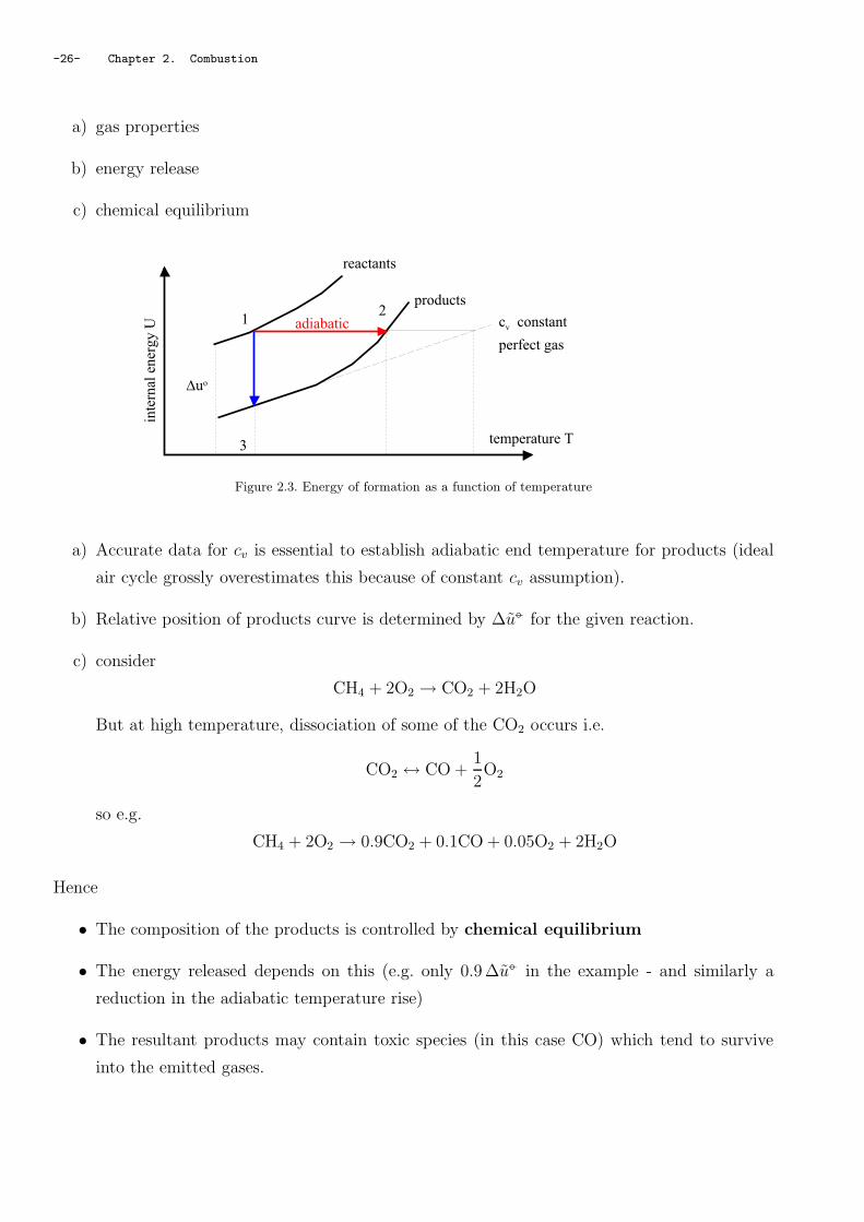
2.2 Combustion Thermodynamics
We need to take account of the effects of high temperatures on:
-26- Chapter 2. Combustion
a) gas properties
b) energy release
c) chemical equilibrium
inte
rnal
ener
gy U
temperature T
cv constant
perfect gas
1
3
2adiabatic
Duo
reactants
products
Figure 2.3. Energy of formation as a function of temperature
a) Accurate data for cv is essential to establish adiabatic end temperature for products (ideal
air cycle grossly overestimates this because of constant cv assumption).
b) Relative position of products curve is determined by ∆u− for the given reaction.
c) consider
CH4 + 2O2 → CO2 + 2H2O
But at high temperature, dissociation of some of the CO2 occurs i.e.
CO2 ↔ CO +1
2O2
so e.g.
CH4 + 2O2 → 0.9CO2 + 0.1CO + 0.05O2 + 2H2O
Hence
• The composition of the products is controlled by chemical equilibrium
• The energy released depends on this (e.g. only 0.9 ∆u− in the example - and similarly a
reduction in the adiabatic temperature rise)
• The resultant products may contain toxic species (in this case CO) which tend to survive
into the emitted gases.
2.3. Criteria for equilibrium -27-
2.3 Criteria for equilibrium
2.3.1 Adiabatic closed system (pure substance)
Mechanical Equilibrium across the system implies uniform pressure
Thermal Equilibrium across the system implies uniform temperature
If both pressure and temperature can change together, the Second Law requires that for any
externally adiabatic process (e.g. mixing between hot and cold parts but with Q = 0):
dS ≥ 0
This (irreversible) process will continue until equilibrium is reached, when S reaches a constant
value, i.e. dS = 0 which is the criterion for equilibrium. This implies that small reversible changes
may take place between components of the system, but the overall condition of equilibrium is not
thereby disturbed.
2.3.2 Isothermal closed system
If system is in mechanical and thermal equilibrium with its surroundings, pressure and temperature
are constant, but there may be some Heat Transfer, Q.
2nd Law now requires:
dS − δQ
T≥ 0
By the same argument as §2.3.1, the criterion for equilibrium is
δQ − TdS = 0
but from 1st Law:
δQ = dU + δW = dU + pdV (when reversible)
Hence
dU + pdV − TdS = 0
But the Gibbs Function G = H − TS = −U + pV − TS for constant pressure and temperature:
dG = dU + pdV − TdS
and at given values of T , p the criterion for equilibrium is:
dG = 0
This applies to any effect at a specified combination of p, T including chemical, phase, electric or
nuclear changes.

-28- Chapter 2. Combustion
2.4 Emissions
• Nitrogen oxides: NO2, NOx
They are formed mainly from road traffic fumes and burning of fossil fuels.
Effects: A respiratory irritant that leads to increases in asthma and susceptibility to infection.
• Carbon monoxide: CO
Mainly due to emissions from vehicle exhausts.
Effects: Toxic and easily absorbed by the blood, blocking oxygen receptors. It causes headaches
and tiredness. Fatal in high concentrations.
• Small particles known as PM10
Tiny particles created by diesel combustion that penetrate deep into the lungs.
Effects: Risk of heart, lung and respiratory diseases. Increased incidence of lung cancer and
cot death.
• Ozone: O3
Effects: irritates eyes, nose and throat, reduces lung capacity and increases asthma and
respiratory diseases.

Chapter 3. Thermodynamics of reacting gas mixtures -29-
Chapter 3: Thermodynamics of reacting gas
mixtures
3.1 Properties of an ideal gas
Properties of an ideal gas with variable cv and cp (i.e. non perfect) (Nicolleau, 2001, )
Equation of state: piV = niRT for each gas i at partial pressure pi
Internal Energy: u = u0 +∫ TT0
cvdT
Enthalpy: h = h0 +∫ TT0
cpdT
For convenience, the tables choose h0 = 0 at T0 = 25C (298 K) and tabulate
h = mh = m∫ T
298cpdT per kmol
and
u = h − RT
(see Rogers & Mayhew, 1998, pp 18-20 for values). Note that all changes in h, u due to chemical
change require the use of
• either the enthalpy of formation ∆h−fo (see Rogers & Mayhew, 1998, p 22)
• or the enthalpy of reaction ∆h− (see Rogers & Mayhew, 1998, p 21)
Entropy:
s = ∆s− − R ln
(p
p−
)J.mol−1.K−1 (3.1)
where p− = 1 bar and
s− =∫ T
0cp
dT
T
depends only on absolute temperature T .
3.2 Gibbs function changes
For a given chemical reaction
naA + nbB = ncC + ndD + ...
∆G = (H − TS)P − (H − TS)R
or, at temperature T
∆GT = na∆h− − T
(∑
P
nisi −∑
R
nisi
)

-30- Chapter 3. Thermodynamics of reacting gas mixtures
Hence ∆GT depends on partial pressures pi of each species in both Products, and Reactants
mixtures because of the si terms as in equation (3.1) above.
The standard gibbs function change ∆G− is the value of ∆GT when each pi is taken as the
standard pressure p− (i.e. all R ln( pi
p−) = 0 in the si terms), and is hence that part of ∆GT which
depends only on the temperature T at which equilibrium is to be considered. Then
∆GT = ∆G− + RT
[∑
P
ni ln
(pi
p−
)−∑
R
ni ln
(pi
p−
)]
3.3 Analysis of chemical equilibrium
Consider the reversible reaction
naA + nbB ⇔ ncC + ndD
to be at equilibrium in a reacting mixture containing A, B, C, D and other species (e.g. N2).
e.g. for CO +1/2 O2 we would have
A as CO na = 1
B as O2 nb = 1/2
C as CO2 nc = 1
For chemical equilibrium, dG = 0, i.e. ∆GT = 0 and hence
∆G− + RT
[nc ln
(pc
p−
)+ nd ln
(pd
p−
)− na ln
(pa
p−
)− nb ln
(pb
p−
)]= 0
Then
−∆G−
RT= ln
[pnc
c pnd
d
pnaa pnb
b
(p−)∆n
]= ln K−
(3.2)
where ∆n = na + nb − (nc + nd) and K−:
is the equilibrium constant for the reaction
is dimensionless
is dependent on T only.
e.g. for CO +12
O2 ⇔ CO2:
K− =pco2
(p−)1
2
pco (po2)
1
2
(3.3)

3.4. Example -31-
Values for ln K− for a range of temperatures are given for some reactions in the tables (see Rogers
& Mayhew, 1998, p 21) or if necessary could be obtained from
ln K− =−∆G−
RT(3.4)
Hence to evaluate the product composition at temperature T in an assumed overall reaction such
as CH4 +2 O2 → a CO2 + b CO + c O2 + 2 H2O
it is only necessary to look up ln K− at temperature T for CO + 1/2 O2 ⇔ CO2 and combine the
element balances for C and O with equation (3.3) to solve for a, b and c.
3.4 Example
a)
A stoichiometric mixture of CO and O2 enters a steady flow burner at 25C and 1 bar. For
combustion at constant pressure calculate
i) the composition of the products when the final exit temperature is 2600 K
ii) the heat transfer from the burner per kmol of CO
a-i)
The overall reaction may be written as:
CO +1
2O2 → xCO + (1 − x)CO2 +
x
2O2
and for equilibrium within the products,
CO +1
2O2 CO2
From tables Rogers & Mayhew (1998), at 2600 K,
ln K− = ln
pco2(1)
1
2
pco(po2)
1
2
= 2.8
Now, since for each species sharing volume V , piV = niRT then
RT
V=
pco
x=
pco2
1 − x=
po2
x2
=pP
nP

-32- Chapter 3. Thermodynamics of reacting gas mixtures
where pP is the total pressure of the products (1 bar) and nP = x + (1 − x) + x2
= 1 + x2
hence
pco = x1+ x
2
pco2= 1−x
1+ x2
po2=
x2
1+ x2
K− = e2.8 =
1−x1+ x
2(x
1+ x2
)(x2
1+ x2
) 1
2
(K−)2x3
2 + x= (1 − x)2
This cubic equation requires iterative solution (initial guess x=0.1, 0.184, 0.175, 0.1762, 0.1761).
Hence%CO: x
nP = 16.2%
%CO2:1−xnP = 75.7%
%O2:x
2nP = 8.1%
a-ii)
Heat transfer
enth
alpy h
temperature T
2
1
Dho
reactants CO, O2
products actual CO, CO2, O2
To = 298 K
ideal CO2
2600
3
3c
Figure 3.1. Example: heat exchange
h1 − h3c = ∆h− = 282990 kJ.kmol−1
but
h1 − h3 = (1 − x)∆h− = 233155 kJ.kmol−1
SFEE: Q = H1 − H2 = (H1 − H3) − (H2 − H3) per kmol of CO. Now
H2 − H3 = x(h2 − h3)co + (1 − x)(h2 − h3)co2
x2(h2 − h3)o2
= 0.1761 × (78714 − 0) + 0.8239 × (128080− 0) + 0.0881 × (82274− 0)
= 126631 kJ.kmol−1 of CO

3.4. Example -33-
Hence
Q = 233115− 126631 = 106524 kJ.kmol−1 of CO
b)
How would the composition of the products differ if the same mixture were obtained in a rigid
vessel and ignited, and the final temperature was again 2600 K?
For combustion at constant volume, p2 6= 1 bar, but since T2 is known, we can use
V = n1RT1
p1= n2
RT2
p2
orp2
n2=
p1
n1
T2
T1=
1
1.5× 2600
298= 5.817 bar/kmol
Hence pco = 5.817x, pco2= 5.817(1 − x), po2
= 5.817x/2 and
(K−)2x3 × 2.9083 = (1 − x)3
try 0.1, 0.101, 0.10091. And n2 = 1 + x2
= 1.0505, p2 = 6.11 bar
%CO = 9.6%
%CO2 = 85.6%
%O2 = 4.8%
c)
Repeat (a) with air in place of O2
If nitrogen is included, the overall reaction becomes
CO +1
2
(O2 +
79
21N2
)→ xCO + (1 − x)CO2 +
x
2O2 + 1.881N2
so nP = 1 + x2
+ 1.881 = 2.881 + x2
and
x3 × 270.43 = (1 − x)2(5.762 + x)
try 0.1, 0.26, 0.23, 0.236, 0.2350, then nP = 2.999
%CO = 7.84%
%CO2 = 25.5%
%O2 = 3.92%
%N2 = 62.7%

-34- Chapter 3. Thermodynamics of reacting gas mixtures
Heat transfer
H1 − H3 = 0.765 × 282990 = 216487 kJ.kmol−1 of CO
H2 − H3 = 126146︸ ︷︷ ︸CO + CO2 + O2
+ 146678︸ ︷︷ ︸N2
= 272824 kJ.kmol−1 of CO
Qout = 216487 − 272824 = −56337 kJ.kmol−1 of CO
Need to heat the flame to reach the 2600C.
3.5 More realistic reactions in engines
In practice
• More chemical species (e.g. H2 , NO, H, O, OH)
• Non stoichiometric reactants.
Example: Methane (CH4) in air
φ CH4 + 2 (O2 + 7921
N2) → a CO + b CO2 + c O2 + d H2O + e H2 + f NO + g N2 + ...
3.5.1 Neglecting NO (f = 0)
a) Lean mixture (φ < 1) assume e = 0 and consider equilibrium within the product mixture of
CO + 12
O2 ⇔ CO2 only
then
C balance φ = a + b
H balance 4φ = 2d
O balance 4 = a + 2b + 2c + d
N balance 47921
= 2g
with pCO
a=
pCO2
b=
pO2
c=
pH2O
d=
pN2
g= p2
n2
n2 = a + b + c + d + g and
K− =pCO2
(p−)1
2
pCO (pO2)
1
2
is the closing equation to solve for the 5 unknown coefficients.
b) Rich mixture (φ > 1) assume c = 0 and consider equilibrium of
H2 + CO2 ⇔ H2O + CO (“water gas” reaction)
As before, 4 balance equations and
K− =pH2O pCO
pH2pCO2
is the closing equation.

3.5. More realistic reactions in engines -35-
3.5.2 With NO concentrations
In order to estimate NO concentrations, we need also to consider equilibrium of12
O2 + 12
N2 ⇔ NO
giving an additional
K− =pNO
(pH2)
1
2 (pCO2)
1
2
i.e. 6 unknowns to be solved from 6 equations (4 element balance equations, 2 equilibrium equa-
tions)
Solution technique: for small concentrations (e.g. of NO) Linear superposition may be approxi-
mately adequate. Hence e.g.
a) solve for case 1-a)
b) use these values to solve for NO as above.
c) Repeat 1-a) with f 6= 0 and iterate.
3.5.3 Exercise
After combustion of a stoichiometric mixture of H2 and O2 in a constant volume bomb, the pressure
of the products is 10 bar, and 5% of the original H2 remains uncombined.
a) Calculate the equilibrium constant K− for the reaction
H2 + 12
O2 ⇔ H2O
assuming no other species are present.
Hence if the initial temperature was 25C, find
b) the temperature after combustion
c) the initial pressure
d) the heat transfer from the reaction per kg original H2
Answers a) 38.5, b) 2844 K, c) 1.53 bar, d) 65 900 kJ.kg−1
3.5.4 Exercise
A spark Ignition engine operates with a 10% rich mixture of octane (C8H18) and air. The exhaust
gases leave the engine at a temperature of 1200 K, at which it may be assumed that the only
significant species are CO2, H2O, CO, H2 and N2. Calculate the wet exhaust composition if it is
also assumed that the following reaction is in equilibrium:

-36- Chapter 3. Thermodynamics of reacting gas mixtures
CO2 + H2 ⇔ CO + H2O
Answers: 11.3% CO2, 2.04 % CO, 13.3 % H2O, 1.76% H2, 71.6% N2
3.5.5 Exercise
In a certain diesel engine cylinder at the end of combustion at maximum load, one quarter of the
initially trapped O2 remains un-reacted, and the mean gas temperature is 2200 K. By assuming
equilibrium of the reaction12
N2 + 12
O2 ⇔ NO
estimate the proportion of the Nitrogen which is converted to NO.
Answers: 0.42%
3.5.6 Exercise
a) A spark ignition engine operates with a 10% rich mixture of carbon monoxide and air. Show
that for equilibrium at 3000 K, 40 bar, about 24% of the CO supplied will remain dissociated,
if only CO, O2, N2, CO2 are assumed present. Hence calculate the molar gas composition.
b) If NO is now considered as a possible additional species, show that the dissociated CO rises
to about 25.7% of that supplied, and that about 1.2% of the Nitrogen supplied is oxidised.
Calculate the new composition.
Answers: a) 27.3% CO2, 8.7% CO, 2.7% O2 and 61.5% N2. b) 26.6% CO2, 9.2% CO, 2.3% O2,
60.5% N2 and 1.4% NO
3.6 Kinetics
The rate at which chemical equilibrium is approached is also dependent on temperature (fast at
high temperature, slow at low temperature). Quantitative analysis of this is too complex for this
course, but qualitative understanding will be important for
a) Ignition.
b) Rate of flame travel.
c) ’Freezing’ during expansion of species formed at high temperature (pollutant emissions).

Chapter 4. Simple physics of flames and combustion -37-
Chapter 4: Simple physics of flames and
combustion
4.1 Premixed laminar flame
In a premixed flame the reactants are well mixed before the flame arrival
The laminar flame front and position are well defined as shown on figure 4.1
burnt gases
products
premixed
reactant
air + fuel
temperature
flame thickness
flame propagation
flame position x
Figure 4.1. Laminar premixed flame
It is then possible from experiment to define the laminar flame speed sl = dxdt
with dx the distance
the flame has moved during a time lag dt. The flame is the result of the equilibrium between three
mechanisms
• There are transfer mechanisms within the flame (exchange of heat, products, reactants)
through a diffusion process. A characteristic time can be based on the diffusion coefficient
κ and the flame thickness δl
τd =δ2
κ
• The flame propagates with a characteristic time based on sl and δl
τa =δl
sl
• The reaction is first of all a chemical reaction and as such is also controlled through chemistry
with its own characteristic time
τch
The laminar flame results of the equilibrium between all these mechanisms:
τd ≃ τa ≃ τch

-38- Chapter 4. Simple physics of flames and combustion
Any change in one of these mechanism may results in the quenching of the flame.
The laminar speed is a function of φ the relative fuel air ratio.
Figure 4.2. Laminar flame speed as a function of φ at 1 bar
4.2 Diffusion flame
• There is no mixing of the reactants before the flame front
• fuel gas and oxygen diffuse from opposite sides
• fuel is heated before oxidation and may decompose → C particle, radical, smoke, soot.
• the combustion is not controlled by overall φ but by mixing
flam
e
airfuel
burntgas
fuel
vapour
airlaminar flame front
Figure 4.3. Diffusion flame

4.3. Detonation Wave -39-
4.3 Detonation Wave
• A shock wave driven by combustion
• not normally possible in engines
4.4 Ignition in Piston Engine
It is necessary to reach a certain temperature for the mixture to ignite this is the ignition phase.
After ignition, the energy released from the combustion will provide the heat necessary to sustain
the combustion.
• Spark ignition: high temperature (e.g. 3000 K) source from an electric discharge (spark).
• Compression ignition: spontaneous1 ignition resulting from high compressed air temperature
(e.g. T = 600 K).
• Pre-ignition: harmful ignition from hot surface during compression stroke.
• Auto-ignition1: spontaneous ignition of ’end gas’ before arrival of the flame resulting in knock
4.5 Turbulent flame
4.5.1 Turbulence parameters
Turbulence can be characterised by
• a velocity macro-scale u′ defined as the rms value of the velocity fluctuations,
• a macro-length scale or integral length scale L corresponding to the size of the largest eddies
present in the turbulent, flow
• a micro-length scale or Kolmogorov length scale ηK corresponding to the small eddies present
in the flow.
4.5.2 Mixing
The flow into the cylinder is highly turbulent and the mean velocity is often smaller than the
turbulent velocity. But by the way air is injected in the cylinder mean flows can also be induced
into the cylinder.
1Time is required to permit initial chain reaction sequence when the flame temperature is low.

-40- Chapter 4. Simple physics of flames and combustion
• Tumble: refers to a rotational flow within the cylinder about an axis orthogonal to the
cylinder axis.
• Swirl: refers to a rotational flow within the cylinder about its axis. Swirl is used in some
gasoline engines to promote a fast burn and is one of two principal means to ensure rapid
mixing between fuel and air in direct-injected diesel or stratified charge engines. Diesel
engines without swirl are said to be quiescent and the intensity of the fuel injection is instead
relied upon to mix the fuel and air. The induction swirl is generated either by tangentially
directing the flow into the cylinder or by pre-swirling the incoming flow by use of a helical
port.
Figure 4.4. Tumble, Swirl and Squish
• Squish: is a radial flow most commonly associated with direct-injection engines in which the
combustion chamber is a cup located within the piston (e.g. figure 4.4 right). The cup is there
to amplify swirl generated during the intake process and squish is a necessary byproduct of
using a cup.
In practice it is impossible to generate swirl without inducing some tumble. The swirl level at the
end of the compression process is dependent upon the swirl generated during the intake process
and how much it is amplified during the compression process.
4.5.3 Turbulent flame front
The first role of turbulence is to increase the mixing of burnt gas with unburn gas which increase
the combustion.
Turbulent flame occurs in turbulent flows, flame front is more complex as in figure 4.5 and flame
speed can not be measured directly. An equivalent turbulent speed sb is calculated based on an
average position of the front as in figure 4.6:

4.5. Turbulent flame -41-
Actual flame compared to the fractal Koch curveby courtesy of Dr D. Queiros-Conde Flame shape as a function of engine speed
from Fergusson (1986)
Figure 4.5. Flame shape in a turbulent flow
Vb Vb
ST
A
Sl
AT
are equivalent
Figure 4.6. Turbulent velocity definition
and mass conservation yields
m = ρuslAT = ρusT A
that is
sT = slAT
A(4.1)
Typically:
3 <sT
sl< 30
Models have been proposed for
sT = sT (u′, L, sl, δl)
for small scale turbulence
sT ≃ sl
(u′
sl
) 1
2

-42- Chapter 4. Simple physics of flames and combustion
For large scale turbulence, the apparent fractal geometry of the flame surface leads to (see Nicolleau
& Mathieu (1994), Nicolleau (1994))
sT ∼ u′
(see Heywood, 1988, figure 9-30 p. 412)The ratio p/pm corrects for the effects ofadditional compressionon the turbulence intensity
(see Peters, 2000, figure 2.22 p. 124)
Figure 4.7. Turbulent flame compared to laminar flame
4.6 Flame Quench
Turbulence also stretches the flame front which can lead to quenching.
A flame may be extinguished
a) near a cold wall
– harmful because unburnt HC remain
– may be necessary to prevent knock
b) In a region where φ is too small (e.g. φ = 0.5)
– Uneven fuel/aire mixing
– stratified charge design
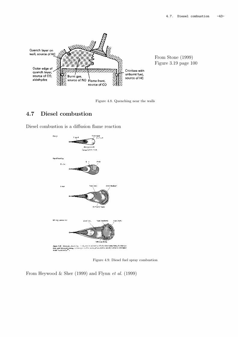
4.7. Diesel combustion -43-
From Stone (1999)Figure 3.19 page 100
Figure 4.8. Quenching near the walls
4.7 Diesel combustion
Diesel combustion is a diffusion flame reaction
Figure 4.9. Diesel fuel spray combustion
From Heywood & Sher (1999) and Flynn et al. (1999)

-44- Chapter 4. Simple physics of flames and combustion
Appendix of chapter 4
4.A Bunsen burner
fuel
airair regulator
premixed flame
air + fuel
diffusion flame
burntgases
airburnt gases
Figure 4.10. Bunsen burner showing premixed and diffusion flames
4.B Turbulent flame propagation
4.C Role of the Swirl

Chapter 5. Equations for reactive flows -45-
Chapter 5: Equations for reactive flows
5.1 Mass conservation of a passive scalar
We define ρ(x, y, z; t) the local instantaneous density
In classical thermodynamics mass cannot be created, destroyed or altered in something else. The
only possibility to change the mass MV inside a given control volume is either
• to add mass to the system or
• to remove mass from the system.
m a s s c o m i n g i n
m a s s g o i n g o u t
Figure 5.1. Mass flux through the surface
That is, the mass variation per unit time inside the control volume between a time t and a time
t + dt is
MV = MV (t+dt)−MV (t)dt
= 1dt
(total mass entering the system during dt
− total mass leaving the system during dt)(5.1)
5.1.1 Mass variation inside a control volume
The mass inside the control volume at time t is
MV (t) =∫ ∫ ∫
Vρ(x, y, z; t) dxdydz
and at time t + dt
MV (t + dt) =∫ ∫ ∫
Vρ(x, y, z; t + dt) dxdydz
so that the mass variation in the control volume is
dMV
dt=∫ ∫ ∫
Vlimdt→0
ρ(x, y, z; t + dt) − ρ(x, y, z; t)
dtdxdydz
that isdMV
dt=∫ ∫ ∫
V
∂ρ
∂tdxdydz (5.2)
Note that on the left hand side there is a total derivative as MV is only a function of time, whereas
on the right hand side it is a partial derivative of ρ that is involved as this latter is a function of
space and time.

-46- Chapter 5. Equations for reactive flows
n
n
n
n
n
V o u t
V i n
Figure 5.2. External normal convention
5.1.2 The notion of flux
The control volume is bounded by a surface and we can define, ~n, the external surface normal. It
is a vector normal to the surface and pointing to the exterior of the control volume.
~V is the matter velocity when it crosses the control surface, then if
• ~V.~n > 0 the matter is leaving the control volume, whereas if
• ~V.~n < 0 the matter is entering the control volume.
So that, for instance, the total budget of mass transfer during dt through the surface can be
formalised as
Mi − Mo = −∫ ∫
Σρ~V.~n dσ dt
(5.3)
and there is no need to discriminate between what is entering and what is leaving the control
volume anymore as this is taken into account by the sign of ~V.~n. Note the minus sign, because
when matter is entering the control volume it is flowing in the direction opposite to the external
normal.
nn
V i n
d s
d l = V i n . n d t
d m = r V i n . n d s d t
s u r f a c e S
I NO U T
t i m e t t i m e t + d t
Figure 5.3. Mass flux through an elementary surface dσ

5.1. Mass conservation of a passive scalar -47-
The quantity ρ~V.~n is called the mass flux.
As shown in figure 5.3, ρ~V.~ndσdt is the elementary element of matter entering the control volume
through the elementary surface dσ.
The same approach is valid for measuring any thermodynamics quantity entering the control
volume. Hence we can define
ρ (~V.~n) mass flow rate,
ρu (~V.~n) internal energy flow rate,
ρh (~V.~n) enthalpy flow rate,
ρ~V (~V .~n) momentum flow rate,
12ρV2 (~V.~n) kinetic energy flow rate ...
5.1.3 The divergence theorem
(For more on the divergence theorem see e.g. Boas, 2005, §10)
There are some cases where it is more interesting to perform an integral over a volume than over a
surface. In some cases we may end up with a mixture of surface and volume integrals. So, it would
be useful to convert a surface integral into a volume integral. The divergence theorem allows one
to perform such a transformation.
The divergence theorem is explicited in figure 5.4, where div( ~A) is called the divergence of ~A and
is defined as
div ~A =∂Ax
∂x+
∂Ay
∂y+
∂Az
∂z(5.5)
in cartesian coordinates with ~A = (Ax, Ay, Az). Note that the definition (5.5) is only valid in
cartesian coordinate though the divergence theorem (5.4) is valid in any coordinate system: it is
an intrinsic definition.
The interest of the theorem is obvious allowing one to replace a vector based integration into a
scalar volume integration. For we have seen that the total mass passing through the control surface
is per unit time (5.3)
Mi − Mo = −∫ ∫
Σρ~V .~n dσ

-48- Chapter 5. Equations for reactive flows
An
d i v A
SV
∫ ∫
Σ︸ ︷︷ ︸surface integration
~A.~n dσ =∫ ∫ ∫
V︸ ︷︷ ︸volume integration
div( ~A) dxdydz (5.4)
Figure 5.4. The divergence theorem
setting ~A = ρ~V the divergence theorem yields:
Mi − Mo = −∫ ∫
Σρ~V .~n dσ = −
∫ ∫ ∫
Vdiv(ρ~V) dxdydz
5.1.4 The continuity equation
Applying mass conservation (5.2) and (5.3) everything can be expressed in terms of volume integral
with no reference to the control surface anymore
∫ ∫ ∫
V
∂ρ
∂tdxdydz = −
∫ ∫ ∫
Vdiv(ρ~V) dxdydz (5.6)
or ∫ ∫ ∫
V
[∂ρ
∂t+ div(ρ~V)
]dxdydz = 0 (5.7)
This latter equation is true whatever the control volume in particular for any small part of the
space, that is for a control volume as small as possible (or V → 0). So that
∂ρ
∂t+ div(ρ~V) = 0
(5.8)
is true at any time and everywhere. (5.8) is called the continuity equation. It is a local version
of the mass conservation. Whatever the mass flow rate, the control surface and volume, equation
(5.8) must be verified at each point (x, y, z) of space.

5.2. Un-reactive mixture -49-
5.2 Un-reactive mixture
In a mixture of different species, further to the global mass conservation (5.8) each species α is
conserved and a demonstration similar to the one done in §5.1.4 leads to
∂ρα
∂t+ div(ρα
~Vα) = 0
(5.9)
where ρα is the density of the αth species:
ρα = xαρ
where xα is the mass fraction of the αth species. Each species has its own density and velocity,
the total mass, momentum and energy are
m =∑
α
mα
ρ~V =∑
α
ρα~Vα
ρu =∑
α
ραuα
ρh =∑
α
ραhα
Then, to solve the problem one needs a momentum and energy equation for each species and these
equations will be all coupled as species are interacting with each other.
5.2.1 The scalar equation
It is possible to work with xα rather than mα, substituting xα in (5.9) yields:
∂ρxα
∂t+ div(ρxα
~Vα) = 0
and after expanding and re-ordering:
xα
[∂ρ
∂t+ div(ρ ~Vα)
]+ ρ
[∂ xα
∂t+ ~grad xα. ~Vα)
]= 0 (5.10)
where ~grad xα is the gradient of xα defined in cartesian coordinate as
~grad xα =
∂ xα
∂x∂ xα
∂y∂ xα
∂z

-50- Chapter 5. Equations for reactive flows
Then noting that∂ρ
∂t+ div(ρ ~Vα) = divρ( ~Vα − ~V) (5.11)
and
divρ xα( ~Vα − ~V) = xαdivρ( ~Vα − ~V) + ρ( ~Vα − ~V). ~grad xα
on gets
ρ∂ xα
∂t+ ρ~V . ~grad xα + divρ xα( ~Vα − ~V) = 0 (5.12)
We can notice that∂ xα
∂t+ ~V . ~grad xα =
∂ xα
∂t+∑
i
Vj .∂xα
∂xj
=dxα
dt
d(xα)dt
is called the particulate or material or total derivative, it is the derivative of the mass fraction
xα along a streamline or following a particle. It is also called Lagrangian derivative.
t = 0t
f l u i d p a r t i c l ef l u i d p a r t i c l e ' s t r a j e c t o r y
i s t a k e n h e r e Figure 5.5. Lagrangian derivative. The derivative is taken where the fluid particle is at time t.
So that (5.12) can be written as
ρd xα
dt+ divρ xα( ~Vα − ~V) = 0
(5.13)
5.2.2 Mass diffusion
If all the species have the same velocity then ~Vα = ~V and
d xα
dt= 0
That is, the mass fraction of the species does not change along a fluid particle trajectory. In
practice, species have different molecular sizes and masses so that there is no reason why they
should move at the same speed. For some ~Vα > ~V , for others ~Vα > ~V, this is called diffusion. As
shown in figure 5.2.2, if for instance ~Vα > ~Vβ, the mass fraction of α will increase faster than the
mass fraction of β. There will be a diffusion of α in β.

5.2. Un-reactive mixture -51-
s u r f a c e c o n t r o l
I N
ab
V a
V b
Figure 5.6. Diffusion effect due to ~Vα > ~Vβ .
divρα(~Vα − ~V)
is the diffusion term that accounts for that effect.
~Φα = ρα(~Vα − ~V)
(5.14)
is the flux of α and is proportional to its velocity departure from the mean velocity.
r e d d i f f u s e s
f l u i d p a r t i c l e ' s t r a j e c t o r y
t
f l u i d p a r t i c l e
X X
t = 0
X Xf l u i d p a r t i c l e
XX f l u i d p a r t i c l e ' s t r a j e c t o r yw h i t e d i f f u s e s
N o d i f f u s i o nW i t h d i f f u s i o n
Figure 5.7. Diffusion effect. On the left, there is no diffusion: the mass fraction of red remains constant on the fluid particle’strajectory. On the right, red and white species diffuse and their mass fractions change along the fluid particle’s trajectory.
It is worth noting that the sum of all fluxes is 0:
∑~Φα = 0 (5.15)
5.2.3 The Fick law
The Fick law states that
~Φα = −ρDα~grad( xα)
(5.16)

-52- Chapter 5. Equations for reactive flows
where Dα > 0 is the mass diffusivity for the species α (in m2 s−1). It represents how fast the
mass of α diffuses through the other species. Equation (5.16) is the definition we will use in these
course. It is worth noting that there is another one which is
~Φα = −D∗α
~grad(ρ xα) (5.17)
Both definitions are not equivalent and it is worth checking which one is used in a textbook. They
are equivalent only when ρ is homogeneous, otherwise (5.17) yields
D∗α
~grad(ρ xα) = D∗αρ ~grad + D∗
αxα~gradρ
and there is a extra term D∗αxα
~gradρ to account for.
To avoid this extra term people interested with mixture use definition (5.16), which from now on
will be what we refer to as the Fick law. The Fick law just states that the species α will diffuse
(=be transferred) from where it is highly concentrated toward where it is weakly concentrated.
D > 0 is the equivalent for concentrations of the zeroth law of thermodynamic. In the case of a
one-dimensional problem (5.16) becomes
Φα = −ρDα∂ xα
∂x
and the Fick law is the equivalent for concentrations of the Fourier law for heat conduction:
qcond. = −k∂T
∂x
where k is the thermal conductivity.
The advantage of using Fick’s law is that equation (5.13) becomes
ρd xα
dt− div(ρDα
~grad( xα)) = 0
(5.18)
~Vα does not appear any more, so that there is no need to solve an equation for each ~Vα anymore.
Only ~V is needed and can be obtained from the Navier-Stokes equations. But (5.16) is nothing
but a closure and as such an approximation, see exercise 5.2.5 to see limitations of the Fick law.
If the flow is homogeneous ρ and Dα do not depend on space and then equation (5.18) can be
simplified into
d xα
dt− Dα ∇2xα = 0
(5.19)
5.3. Reactive scalar -53-
where ∇2xα = ∂2 xα
∂x2 + ∂2 xα
∂y2 + ∂2 xα
∂z2 is the Laplacian of xα.
For sake of simplicity it is often assumed that the mass diffusivity Dα is proportional to the
thermal diffusivity kα/ρcp (m2 s−1):
Dα ∝ kα
ρcp
kα is the thermal conductivity and cp the heat capacity. The thermal diffusivity represents how
fast heat diffuses through the phase α. The ratio of the thermal diffusivity to the mass diffusivity
is called the Lewis number:
Leα =
kα
ρcp
Dα=
kα
ρcpDα
(5.20)
5.2.4 Exercise
Derive equation (5.10) and show (5.11) and (5.12)
5.2.5 Exercise
Derive the property (5.15). Then using the property that∑
xα = 1, show that if all the Dα are
equal then (5.15) is verified.
Then show that only when all the Dα are equal (5.15) is verified.
5.2.6 Exercise
A greasy plate is placed into the water, and a thin film of oil forms on top of the water. Find the
flux, J in mol cm2 s−1, of oil droplets through the water to the top surface. The sink is 18 cm
deep, and the concentration of oil on the plate is 0.1 mol cm−3. Assume that there is no oil at the
top of the sink yet.
5.3 Reactive scalar
For a reactive mixture, mass still cannot be created or destroyed and equation (5.8) is still valid.
But this is not true of equation (5.9) as a given species can be destroyed or created this is precisely
what happens in a chemical reaction.
So that the mass Mα of the species α inside a given control volume can be altered by
• adding mass of α to the system or
• removing mass of α from the system or

-54- Chapter 5. Equations for reactive flows
• creating or destroying the species α
A term of production needs to be added to (5.9), we define τα the specific production rate of α
(i.e. in kg m−3 s−1)
ρd xα
dt− div(ρDα
~grad( xα)) = τα
(5.21)
That is
ρd xα
dt= div(ρDα
~grad xα)︸ ︷︷ ︸
diffusion
+ τα︸︷︷︸production
5.4 The energy conservation
• As for mass, energy can be altered by transfer or flux of matter. Any matter transferred
inside the control volume has a certain energy that will be added to the energy previously
contained in the control volume.
e n e r g y w i t h m a s s c o m i n g i n
e n e r g y w i t h m a s s g o i n g o u t
a) Energy entering and leavingthe control volume with mass transfer
Q
W
b) Closed system,1st law of thermodynamic
Figure 5.8. Altering energy in a control volume
• But by contrast to mass, this is not the only mechanism by which energy can be altered.
According to the first of thermodynamic, energy can be altered by adding heat or work to
the system; this can be done without matter entering or leaving the control volume.
So that a general formulation of the first law of thermodynamic for an unsteady system is
∆U = U(t + dt) − U(t) = Uf − Ui = Uin − Uout + Win + Qin
(5.22)
5.4. The energy conservation -55-
Q i n
m a t t e r i n
W i n
m a t t e r o u t( U i n ) ( U o u t )
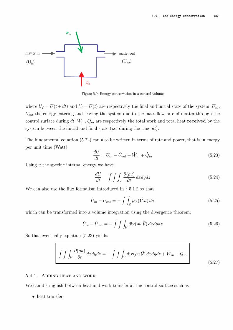
Figure 5.9. Energy conservation in a control volume
where Uf = U(t + dt) and Ui = U(t) are respectively the final and initial state of the system, Uin,
Uout the energy entering and leaving the system due to the mass flow rate of matter through the
control surface during dt. Win, Qin are respectively the total work and total heat received by the
system between the initial and final state (i.e. during the time dt).
The fundamental equation (5.22) can also be written in terms of rate and power, that is in energy
per unit time (Watt):dU
dt= Uin − Uout + Win + Qin (5.23)
Using u the specific internal energy we have
dU
dt=∫ ∫ ∫
V
∂(ρu)
∂tdxdydz (5.24)
We can also use the flux formalism introduced in § 5.1.2 so that
Uin − Uout = −∫ ∫
Σρu (~V.~n) dσ (5.25)
which can be transformed into a volume integration using the divergence theorem:
Uin − Uout = −∫ ∫ ∫
Vdiv(ρu ~V) dxdydz (5.26)
So that eventually equation (5.23) yields:
∫ ∫ ∫
V
∂(ρu)
∂tdxdydz = −
∫ ∫ ∫
Vdiv(ρu ~V) dxdydz + Win + Qin
(5.27)
5.4.1 Adding heat and work
We can distinguish between heat and work transfer at the control surface such as
• heat transfer

-56- Chapter 5. Equations for reactive flows
• pressure force on the surface
• shear force on the surface
and internal work and heat production e.g.
• chemical reaction
• potential energy variation due to body force as gravity
As we did before we can define fluxes and use the divergence theorem to replace what happens at
the surface with something that can be computed in the volume.
• The heat flux ~qσ is defined as the surface density of heat transferred at the surface in a
certain direction. Its unit is J m−2.
q s
n
Figure 5.10. Heat flux
The total amount of heat transferred to the system through the surface during dt is
QΣ = −∫ ∫
Σ~qσ.~ndσ =
∫ ∫ ∫
Vdiv~qσ dxdydz
or in terms of heat flow rates:
QΣ = −∫ ∫
Σ
(∂
∂t~qσ
).~ndσ = −
∫ ∫ ∫
Vdiv
(∂
∂t~qσ
)dxdydz
(5.28)
where QΣ is the total amount of heat rate transferred to the system through the surface, its
unit is W; ∂∂t
~qσ is the heat flux rate, its unit is W m−2.
• The pressure applied to a fluid particle in motion results in a work. The elementary power
due to the pressure applied over a small portion dσ of the surface is
δWpressure = p dσ ~n︸ ︷︷ ︸pressure force
.~V (5.29)

5.4. The energy conservation -57-
where ~V is the fluid particle’s velocity when it crosses the control surface. Note also that
dσ ~n.~Vdt = dV , the volume variation, so that (5.29) is just another form of the pressure
work W = −pdV . Therefore, the total power over the whole surface due to pressure is
Wpressure = −∫ ∫
Σp~V.~n dσ = −
∫ ∫ ∫
Vdiv(p~V) dxdydz
(5.30)
• In general the force applied on the surface can be decomposed into a normal component
(pressure) and a tangential component (shear force):
n
FI N
s u r f a c e
p r e s s u r e p . nI N
s u r f a c e
shear
t
Figure 5.11. Shear and pressure forces
The shear force direction is orthogonal to the normal ~n so that it can be modelled as
~τ = τ .~n (5.31)
where τ is the stress tensor. With this formalism the divergence theorem yields
Wshear = −∫ ∫
Σ(τ .~n).~V dσ = −
∫ ∫ ∫
Vdiv(τ .~V) dxdydz
(5.32)
5.4.2 Volume force
A typical volume force or body force, ~Fb, is the weight, for an elementary volume dV = dxdydz
~Fb = dm~g = ρ dV ~g
It does not depend on the surface and applies at any point inside the control volume. The power
of the body force is then given by
Wb =∫ ∫ ∫
V
~Fb.~V dxdydz

-58- Chapter 5. Equations for reactive flows
that is for gravity
Wb =∫ ∫ ∫
Vρ~g.~V dxdydz
(5.33)
5.4.3 Heat production
Similarly, we can define a volume heat power, this would typically be a chemical reaction or
radiation. If a chemical reaction is occurring in the control volume, from a thermodynamic point
of view this results in a heat power production everywhere in the control volume:
Qprod︸ ︷︷ ︸Total heat produced
in the volume
per unit time (W)
=∫ ∫ ∫
Vqprod︸ ︷︷ ︸
local
heat production rate
(W m−3)
dxdydz
(5.34)
5.4.4 The energy balance
Having described the different contributions to Win and Qin we can now explicit equation (5.27):∫ ∫ ∫
V∂(ρu)
∂tdxdydz = − ∫ ∫ ∫
V div(ρu.~V) dxdydz
due to matters entering the control volume
− ∫ ∫ ∫V div(p.~V) dxdydz
pressure work on the surface
+∫ ∫ ∫
V div(τ .~V) dxdydz
shear force on the surface
+∫ ∫ ∫
V ρ(~g.~V) dxdydz
volume force (weight)
− ∫ ∫ ∫V div(~q) dxdydz
heat transfer at the surface
+∫ ∫ ∫
V qprod dxdydz
heat produced in the volume
(5.35)

5.4. The energy conservation -59-
Which leads to the local internal energy equation:
∂(ρu)
∂t+ div(ρu.~V) = −div(p.~V) + ρ(~g.~V) + div(τ .~V) − div(~q) + qprod
(5.36)
5.4.5 Enthalpy conservation
Engineers are more interested in the net work when the decanting energy has been removed from
Wnet. This can be obtained from the enthalpy definition:
h = u + pv = u +p
ρ
so that equation (5.36) becomes
∂
∂t
(ρ(u +
p
ρ)
)+ div(ρu.~V) + div(ρ
p
ρ.~V) =
∂p
∂t+ ρ(~g.~V) + div(τ .~V) − div(~q) + qprod
that is
∂
∂t(ρh) + div(ρh.~V) =
∂p
∂t+ ρ(~g.~V) + div(τ .~V) − div(~q) + qprod
(5.37)
or using property (5.4.7)
ρd
dth =
∂p
∂t+ ρ(~g.~V) + div(τ .~V) − div(~q) + qprod (5.38)
5.4.6 Total enthalpy
If compared to the enthalpy h, the kinetic energy is significant it has to to be accounted for and
it is
ρ(h +1
2V2) = total enthalpy
that is conserved. The demonstration can be conducted with ρ(h + 12V2) instead of h this leads to
the total-enthalpy local equation:
d
dt
(ρ(h +
1
2V2)
)=
∂p
∂t+ ρ(~g.~V) + div(τ .~V) − div(~q) + qprod (5.39)
5.4.7 Exercise
Show that∂
∂t(ρA) + div(ρA.~V) = ρ
∂A
∂t+ ρ~V. ~gradA = ρ
dA
dt
where A is a scalar function.

-60- Chapter 5. Equations for reactive flows
5.5 Energy equation for a reacting mixture
In the case of a mixture the enthalpy of the mixture is defined as
h =∑
ραhα
the momentum of the mixture is
ρ~V =∑
ρα~Vα
but
ρh.~V 6= ραhα.~Vα
because this flux describes the transfer on a surface and is not an extensive or additive quantity.
5.5.1 Exercise
Prove that
ρh.~V 6= ραhα.~Vα
5.5.2 Energy conservation for a mixture
Hence it is safer to work on the basics energy conservation principle (5.23):
dU
dt= Uin − Uout + Win + Qin (5.40)
as whether we are dealing with a single phase or a mixture (5.23) holds. There is no need to make
special case for dUdt
as U is an extensive quantity, so that for a mixture
dU
dt=∑
α
d
dtUα
Win, Qin can be dealt with as they where before. But Uin − Uout needs to be looked at carefully
it is now accounting for the flux of each species α moving through the surface that is
Uin − Uout = −∑
α
∫ ∫
Σραuα(~Vα.~n)dσ
The divergence can still be applied and
Uin − Uout = −∫ ∫ ∫
V
∑
α
div(ραuα.~Vα)dxdydz
So that equation (5.27) becomes
∫ ∫ ∫
V
∑
α
∂(ραuα)
∂tdxdydz = −
∫ ∫ ∫
Vdiv
∑
α
(ραuα~Vα) dxdydz + Win + Qin
5.5. Energy equation for a reacting mixture -61-
Win, Qin can be replaced by they previous expression which do not involve a break down in
different species, so that equation (5.36) which was only valid for a single-phase flow has to be
replaced by
∂
∂t
∑
α
ραuα + div(∑
α
ραuα.~Vα) = −div(p.~V) + ρ(g.~V) + div(τ .~V) − div(~q) + qprod (5.41)
for a mixture. This latter equation can be re-arranged to get an equation in terms of the total
derivative of the specific energy ddt
u. First, we can notice that the second term of (5.41) can be
re-organised as
div(ραuα.~Vα) = divραuα.(~Vα + ~V − ~V)
= div(ραuα.~V) + div(uαΦα)
where we use (5.14) the definition of the flux of α. So that the left hand side of (5.41) can be
re-written as follows
∂
∂t
∑
α
ραuα + div(∑
α
ραuα.~Vα) =∂
∂t
∑
α
ραuα + div(∑
α
ραuα.~V) + div(∑
αuαΦα)
that is
∂
∂t
∑
α
ραuα + div(∑
α
ραuα.~Vα) =∑
α
∂
∂t(ρxαuα) + div(ρxαuα.~V) + div(uαΦα)
(5.42)
We can now apply (§5.4.7) to A = xαuα:
ρd
dt(xαuα) =
∂
∂t(ρxαuα) + div(ρxαuα.~V) = ρ
∂
∂t(xαuα) + ρ~V . ~grad(xαuα) (5.43)
and use this in (5.42):
∂
∂t
∑
α
ραuα + div(∑
α
ραuα.~Vα) =∑
α
ρ
d
dt(xαuα) + div(uαΦα)
= ρ
d
dt
∑
α
xαuα + div(∑
α
uαΦα)
Eventually, this leads to the expression for the total energy we were looking for
∂
∂t
∑
α
ραuα + div(∑
α
ραuα.~Vα) = ρd
dtu + div(
∑
α
uαΦα)
Which can in turn can be substituted in (5.41) to yield
ρd
dtu + div(
∑
α
uαΦα) = −div(p.~V) + ρ(g.~V) + div(τ .~V) − div(~q) + qprod (5.44)
or
ρd
dtu = −div(~q +
∑
α
uαΦα) − div(p.~V) + ρ(g.~V) + div(τ .~V) + qprod
(5.45)
which is the equation for the specific energy u of a mixture of α species. In this equation qprod is
actually the heat produced by radiation as the chemical energy is accounted for in u =∑
xαuα
which is the combination of energies of reactants and products. Radiation is the only heat that
can be produced by other mechanisms. For the sake of clarity we will therefore replace qprod by
qrad.

-62- Chapter 5. Equations for reactive flows
5.5.3 Exercise
Show that
ρd
dt(xαuα) = ρ
∂
∂t(xαuα) + ρ~V. ~grad(xαuα) =
∂
∂t(ρxαuα) + div(ρxαuα.~V)
andd
dt(ρxαuα) =
∂
∂t(ρxαuα) + ~V . ~grad(ρxαuα) =
∂
∂t(ρxαuα) + div(ρxαuα.~Vα)
Starting from (5.45) show that the equation for the energy per unit volume can be written as
d
dt(ρu) = −ρu div~V − div(~q +
∑
α
uαΦα) − div(p.~V) + ρ(g.~V) + div(τ .~V) + qrad
5.6 Enthalpy conservation for a reactive mixture
We can use the same trick we used in (5.37) with (5.45)
ρd
dth =
∂p
∂t− div(~q +
∑
α
hαΦα) − div(p.~V) + ρ(g.~V) + div(τ .~V) + qrad
(5.46)
which is the equation for the specific enthalpy h of a mixture of α species. Again if the kinetic
energy is significant h must be replaced by h + 12V2.
5.6.1 Exercise
Derive equation (5.46) from (5.45).
5.7 Heat transfer
5.7.1 Heat transfer through mass transfer
It is worth taking some time to understand the term∑
α uαΦα in equation (5.45). It is the only ad-
ditional term to the energy equation obtained for a single phase (5.36). We have seen (figure 5.2.2)
that a difference in species’ velocity will result in altering the mass fraction of the different species.
Now, if the different species have different energies they will alter the energy inside the control
volume.
As illustrated in figure 5.7.1, the temperature inside the control volume can be increased by putting
more of a warm species than of a cooler species. There is a transfer of energy that is just due to

5.7. Heat transfer -63-
s u r f a c e c o n t r o l
I N
ab
V a
V b
i f T a > T b , T i n w i l l i n c r e a s e
s u r f a c e c o n t r o l
I Nab
V a
V b
i f T a > T b , T i n w i l l d e c r e a s e
Figure 5.12. Heat transfer due to mass transfer.
the fact that ~Vα 6= ~Vβ . Hence
∑
α
uαΦα
(5.47)
is the heat flux associated to a mass transfer. It is equal to 0 if
• all species have the same velocity, then Φα = 0,
• all species have the same energy uα (as∑
Φα = 0).
This term corresponds to a heat transfer and not to a work transfer because it is a 100% irreversible
process: once the species are mixed they cannot be unmixed.
5.7.2 Modelling of the total Heat transfer
~Ψ = ~q︸︷︷︸conduction
+∑
α
hαΦα
︸ ︷︷ ︸heat flux due to mass transfer
(5.48)
is the total heat flux. We can use Fourier’s law
~q = −k ~gradT
and Fick’s law
Φα = −ρDα~grad xα
then
~Ψ = −k ~gradT −∑
α
ρDαhα~grad xα (5.49)

-64- Chapter 5. Equations for reactive flows
The Fourier law has introduced the temperature which is not an independent variable as it is
linked to the enthalpy. Indeed we have
h =∑
α
xαhα
We can make the assumption a perfect gas, that is for each species
hα = cp αT
where cp α is the specific heat capacity associated to α and is constant, then we can calculate cp
as
h = cpT =∑
α
xαcp αT (5.50)
that is
cp =∑
α
xαcp α
cP is not constant but a function of the mass fractions xα. Then from (5.50) we get a simple
expression for ~gradT as a function of h:
~grad h =∑
α
T ~grad (cp αxα) + cp αxα
~grad T
= cp~gradT +
∑
α
cp αT ~grad (xα)
that is
~gradT =1
cp
~gradh −∑
α
hα
cp
~gradxα
and (5.49) becomes
~Ψ = − k
cp
~grad h +∑
α
khα
cp
~grad xα −∑
α
ρDαhα~grad xα
that is:
~Ψ = − k
cp
~gradh +∑
α
hα
k
cp− ρDα
~grad xα
(5.51)
or introducing the Lewis number:
~Ψ = − k
cp
(~gradh −
∑
α
hα
1 − 1
Leα
~grad xα
)(5.52)
The assumption that Leα = 1 is often made, that means that the thermal diffusivity is equal to
the mass diffusivity, in other word mass diffuses as fast as heat. Under this assumption
~Ψ = − k
cp
~gradh

5.8. Momentum equation -65-
which does not depend on hα any more and (5.46) becomes
ρd
dth =
∂p
∂t+ div
(k
cp
~gradh
)− div(p.~V) + ρ(g.~V) + div(τ .~V) + qrad
(5.53)
which does not make explicit references to α any more, but it is worth noting that cp =∑
α xαcp α
is not a constant but a function of xα.
5.8 Momentum equation
The equations we derived for the energy involves the velocity, an equation for the velocity can be
derived from the momentum equation.
Momentum ρ~V∂
∂t(ρVi) + Vj
∂
∂xj
(ρVi) = ρFi −∂p
∂xi
+∂
∂xj
(τij) (5.54)
Please refer for example to MEC404, MEC311 for more on momentum and Navier-Stokes equa-
tions.

-66- Chapter 5. Equations for reactive flows

Revision questionnaire of Part I -67-
Revision questionnaire of Part I
1) What is the specific fuel consumption sfc?
2) What are the equivalence ratio φ, the excess air ratio λ, what do they measure?
3) Explain the difference between premixed and diffusion laminar flame
4) Explain what are tumble, swirl and squish.
5) What are the effects of turbulence in a piston engine?
6) What is Fick’s law?
7) Explain what the Lewis number is.
8) Explain the physical meaning of each term in
ρd xα
dt− div(ρDα
~grad(ρ xα)) = τα
9) Explain the physical meaning of∑
α
uαΦα
in the energy balance of a reactive mixture:
ρd
dt(ρu) = −div(~q +
∑
α
uαΦα) − div(p.~V) + ρ(g.~V) + div(τ .~V) + qrad

-68- Revision questionnaire of Part I

part II: Piston engines -69-
Part II
Piston engines

-70- part II: Piston engines

Chapter 6. Piston engines -71-
Chapter 6: Piston engines
(Cengel & Boles, 1998, §8.3 8.5)
6.1 Performance Parameters for Piston Engines
6.1.1 Swept volume
Bore B
sweptvolume
displacementvolume
clearance volume
strokeS
Figure 6.1. Swept volume for one cylinder
For nc cylinders the swept volume is
Vs = ncπ
4B2S
(6.1)
6.1.2 Torque
If τ is the crankshaft torque, the work done per revolution (i.e. per two strokes) is
W = 2πτ(6.2)
6.1.3 Power
if the engine rotates at N rev.min−1 the power W is
W = W × N
60= 2πτ
N
60(6.3)

-72- Chapter 6. Piston engines
6.1.4 Volumetric efficiency, ηvol
the volumetric efficiency, ηvol, relates the amount of air, trapped in the cylinder when the inlet
valve closes (IVC), to the cylinder capacity or Swept Volume, Vs. Although this is in principle a
ratio of volumes, it is defined in terms of the mass of air trapped because the volume trapped may
contain fuel vapour or products of combustion as well as air, and the pressure and temperature
at IVC are probably not known. Hence
ηvol =ma
ρaVs
(6.4)
where ρa is the air density at the cylinder inlet (or engine intake).
If a complete cycle requires ns strokes of the piston (2 or 4 stroke), then the air mass flow rate is
ma = ηvolρaVsN
30 ns
= αmf (6.5)
as air is injected every ns (2 or 4) strokes. So that from (1.1)
W = ηthηvolρa
αVs
N
30 nsLCV (6.6)
6.2 Mean effective pressure
It is helpful to define several quantities that we will call mean effective pressures.
A mean effective pressure is the constant pressure which, acting on the piston area through
the stroke, would produce the observed work per cycle.
This pressure is a fiction, but a useful one. During a real cycle the pressure is only significant
during the compression and power strokes. During the compression stroke work is done on the gas
in the cylinder, while during the power stroke the gas in the cylinder does work on the piston.
Hence, the net pressure would be the difference between these two. The mean effective pressure
is therefore the difference between the average pressures on the power and compression strokes.
pm is an average pressure on the piston so that per cycle
Wcy = pmVs
6.2.1 Brake mean effective pressure pm
The most common mean effective pressure is the brake mean effective pressure, bmep or
pbm. The adjective brake refers to measurement at the flywheel. Originally, power output was

6.2. Mean effective pressure -73-
stroke S
swept volume
atmospheric pressure pa
atmospheric pressure pa
mean effective pressure pm
clearance volume Vc
maximum volumeVmax
The net work output of a cycle
Wcy =∫
pdv
is equivalent to the product ofthe mean effective pressure pm
and the swept volume
Wcy = pmVs
Figure 6.2. Mean effective pressure pm
measured by applying an ordinary brake to the flywheel, the brake being attached to a long arm,
and the moment produced was measured.
Brake power simply means power including the effects of mechanical inefficiency - that is, loss of
power to pumping, valve gear, certain accessories and friction.
The work and power from the crankshaft are called brake values Wb, and Wb. So that per cycle
Wb = pbmVs = nsπτ
where pbm is the brake mean effective pressure and so
pmb =nsπτ
Vs
(6.7)
Also
W = pmVsN
30 ns
(either brake or indicated) and using (6.6):
pm = ηthηvolρa
αLCV
pbm is useful because it is roughly comparable even in very different engines, as these different
engines burn the same fuel, necessarily under approximately the same conditions, and hence gen-
erate similar pressures.

-74- Chapter 6. Piston engines
Differences in pbm represent genuine design differences, and not irrelevant differences such as size.
pbm is mainly linked to the engine ability to ‘breathe’ - as we will see in chapter 11 - and is in prac-
tice limited by present techniques to manage mechanically and thermally with high heat capacities.
6.2.2 Indicated mean effective pressure pmi
A indicated mean effective pressure or pmi can also be defined in the cylinder, rather than
at the flywheel. It will be referring to the internal or indicated work i.e.
Wi = pmiVs
By definition pmi does not contain the effects of mechanical friction, or the work necessary to
pump the gases in and out and drive the camshaft and various accessories. It consequently will be
somewhat higher than the brake value pbm.
6.2.3 Mechanical efficiency
When we consider friction, we can define a friction mean effective pressure, or pfm, which is
defined using the power expended on friction.
pbm = pm − pfm
(6.8)
That is: the brake work (what you actually get) is the difference between the indicated work (what
you think you should get) and the frictional losses. This leads to the definition of the mechanical
efficiency
ηmech =Wb
Wi
=Wb
Wi
=pmb
pmi
=ηthb
ηthi
=isfc
bsfc
(6.9)
(≃ 80% at full load).
6.3 Exercise
a) At full load, an automotive engine running on gasoline (LCV= 44 000 kJ.kg−1) at an air/fuel
ratio of 15.0 operates with 35 % brake thermal efficiency and 80 % volumetric efficiency. For air
intake conditions of 0.975 bar, 10C, what are the equivalent brake mean effective pressure and
brake specific fuel consumption?

6.3. Exercise -75-
b) For a 2 litre 4-stroke engine, find the corresponding torque at the flywheel.
c) For a speed of 3000 rev.min−1, find the brake power.
d) If the same engine is converted to run on natural gas mixed with the intake air in the ratio
1:10 by volume, estimate the new volumetric efficiency.
answers a) 9.9 bar, 0.234 kg.kWh−1, b) 157 Nm, c) 49.3 kW, d) 73 %

-76- Chapter 6. Piston engines
Appendix of chapter 6
6.A Piston engine survey
A 1998-2000 cars - derived from data in Automotive Engineering International (SAE)
and Automotive Engineer (IMechE)
engine swept comp. at maximum power Max. torque
type volume ratio Vp∗ bmpe bmpe
litre kW.lit−1 m.s−1 bar Nm bar
Naturally aspirated
Chrysler Jeep Power Tech V8 sohc4 4.7 9.3 37.2 13.8 9.3 400 10.7
Ford Mustang V6 ohv 3.8 9.0 37.5 15.0 8.56 271 9.0
———— GT V8 dohc 4.8 9.0 35 14.5 8.84 393 10.3
———— SVT Cobra V8 dohc 4.8 9.85 50 18.3 9.96 427 11.2
GM Opel ECOTEC IL4 dohc 2.2 9.5 49 18.7 9.9 203 11.6
Toyota 1 SZ-FE VVT IL4 dohc 0.98 10.0 52.4 13.3 10.5 95 12.2
Alfa Romeo twin spark IL4 dohc 1.8 10.3 60.7 17.9 11.2 169 12.2
——————— IL4 dohc 2.0 10.0 57.9 19.4 10.85 187 11.9
——————— V6 dohc 2.5 10.3 56.2 14.3 10.7 222 11.2
Jaguar AJ V6 dohc 3.0 10.5 60.3 18.0 10.7 300 12.7
BMW M5 V8 dohc 4.9 11.0 59.5 19.6 10.8 500 12.7
Renault F5R GDI IL4 dohc5 2.0 51.5 16? 11.2 200 12.6
Turbocharged
Ford Endura Dl diesel IL4sohc 1.8 37.2 11 11.2 200 14.0
Chrysler Jeep diesel ILS sohc2 3.1 21 35.8 12.5 10.8 373 15.0
Maserati V8 dohc 3.2 84.7 16.7 16.3 442 17.4
Audi TT Spark ignition IL4 dohc5 1.8 8.9 92 15 19.6 280 19.6
B Medium speed (turbocharged and intercooled, max 1000 rev/min - not for cars!)
Alsthom 20RK270 V20 ohv 350 13.3 17.1 10.2 20.6 57400 20.6
ohv overhead valves (i.e. push rod operated)
sohc single overhead camshaft (2 or 4 valves/cylinder)
dohc double overhead camshafts (4 valves/cylinder unless 5 shown)
Vp∗ mean piston speed

Chapter 7. Spark ignition engines -77-
Chapter 7: Spark ignition engines
7.1 Ideal Otto cycle (Beau de Rochas)
Assume:
• Working fluid is a perfect gas (pv = RT , constant cv and γ)
• Closed system with external heat transfers at constant volume
• Reversible processes, compression and expansion adiabatic.
Otto cycle is composed of four internally reversible processes:
1-2 isentropic compression
2-3 constant volume heat addition
3-4 isentropic expansion
4-1 constant volume heat rejection
clearance volume Vc
swept volume Vs
volume V
1
2
3
4
1
2
3
4
entropy s
tem
per
ature
Q23
cooling Q14
combustionwork output W
Figure 7.1. Otto Cycle
We can define the compression ratio rv
rv =V1
V2=
Vs + Vc
Vc= 1 +
Vs
Vc
(7.1)

-78- Chapter 7. Spark ignition engines
For compression (1 - 2) and expansion (3 - 4) processes, the entropy s is constant and hence:
T2
T1
=(
V1
V2
)γ−1
= rvγ−1 =
(V4
V3
)γ−1
=T3
T4
Net cycle work
Wnet = W3−4 + W1−2 = U3 − U4 + U1 − U2 = mcv(T3 − T2 − (T4 − T1))
Heat input
Q2−3 = mcv(T3 − T2)
Cycle efficiency
ηc =Wnet
Q2−3= 1 − 1
rvγ−1
(7.2)
Hence:
1) Wnet depends on: m, (T3 − T2), rv, γ
2) ηc depends mainly on rv (i.e. mean temperature separation between heating and cooling)
From Heywood (1988)figure 5-19 page 197.
Efficiency ηth
as a function of the compression ratio rv
−−− ideal gas constant volume cycle− fuel air cycle(12), (13), (14) engine data
Figure 7.2. Otto cycle efficiency
7.2. Realistic thermodynamic cycles -79-
7.1.1 Exercise
An engine works on the ideal Otto cycle with a compression ratio of 10 and a maximum cycle
pressure of 100 bar. The initial conditions are 1 bar, 300K.
a) Assuming that the working fluid is ideal air (γ = 1.4, cv = 0.7178 kJ.kg−1.K−1) calculate
i) The cycle efficiency
ii) the maximum gas temperature
iii) the heat input required per kg air
iv) p, T at the end of the expansion stroke
v) the mean effective pressure pm
b) Repeat i) and iii) above but use values of γ and cv for air appropriate to the mean T of the
heat input process.
c) Compare the results of both a) iii) and b) iii) above with the chemical energy available per kg
air from combustion of a stoichiometric mixture of octane and air at 298 K.
Answers a) 60.2 %, 3000K, 1612 kJ, 3.98 bar, 1194 K, 11.28 bar, b) 49.9 %, 2142 kJ c) 2964 kJ
7.2 Realistic thermodynamic cycles
7.2.1 Effects of fuel-air Otto cycle
a) Non ideal gas: cp, cv, γ are not constant but functions of temperature (γc 6= γe).
b) Real chemistry effects
– gas composition changes
– equilibrium gives effect of φ on :power (maximum for 1.1 < φ < 1.2)
economy (best for 0.8 < φ < 0.9)
c) Hence magnitudes of mep and cycle efficiency both substantially less than for ideal air Otto
cycle
7.2.2 Effects of departure from constant volume
a) Combustion: flame travel requires finite time.
b) Gas Exchange: exhaust blow-down and air intake processes benefit from extended periods
of valve opening
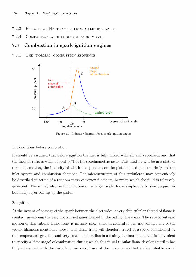
-80- Chapter 7. Spark ignition engines
7.2.3 Effects of Heat losses from cylinder walls
7.2.4 Comparison with engine measurements
7.3 Combustion in spark ignition engines
7.3.1 The ’normal’ combustion sequence
unfired cycle
degree of crack angle-60 60120 tdctop dead center
10
50
pre
ssure
p (
bar
)
A
B
C
first stage of combustion
secondstageof combustion
Figure 7.3. Indicator diagram for a spark ignition engine
1. Conditions before combustion
It should be assumed that before ignition the fuel is fully mixed with air and vaporised, and that
the fuel/air ratio is within about 30% of the stoichiometric ratio. This mixture will be in a state of
turbulent motion, the intensity of which is dependent on the piston speed, and the design of the
inlet system and combustion chamber. The microstructure of this turbulence may conveniently
be described in terms of a random mesh of vortex filaments, between which the fluid is relatively
quiescent. There may also be fluid motion on a larger scale, for example due to swirl, squish or
boundary layer roll-up by the piston.
2. Ignition
At the instant of passage of the spark between the electrodes, a very thin tubular thread of flame is
created, enveloping the very hot ionised gases formed in the path of the spark. The rate of outward
motion of this tubular flame front is initially slow, since in general it will not contact any of the
vertex filaments mentioned above. The flame front will therefore travel at a speed conditioned by
the temperature gradient and very small flame radius in a mainly laminar manner. It is convenient
to specify a ’first stage’ of combustion during which this initial tubular flame develops until it has
fully interacted with the turbulent microstructure of the mixture, so that an identifiable kernel

7.4. Knock in Spark ignition Engines (’Spark Knock’, ’Pinking’, ’Detonation’) -81-
of flame is established. Since the proportion of the mixture involved in this stage is negligible, no
overall change in cylinder pressure is observable, above that due to piston compression alone.
3. Flame propagation
The interaction of the flame with the fluid turbulence results in very much faster combustion,
because both combustion products are rapidly mixed with unburnt fuel and air. The combustion
process thus takes place over a thick belt containing pockets of unburnt mixture in a matrix of
burning gas. This belt itself propagates progressively through the combustion chamber from the
initial kernel. Externally, this belt will however appear as a fairly well defined but rough flame
surface, which expands like a convoluted wrinkled balloon. The sharp temperature rise at this
flame surface can be detected at any point in the chamber at the instant of its arrival, for example
by an ionisation probe or by a suitably placed optical detector.
This process may be regarded as a second stage of combustion, during which the observable
pressure rise occurs.
4. Time required
Although there is no physically definable instant at which the first stage terminates and the second
stage begins, it is convenient to use the approximate point at which the cylinder pressure curve
departs from the equivalent compression curve for this purpose, as indicated by Ricardo (point B
in hie fig. 1.1). The time required for the first stage is highly dependent on the laminar flame speed
and hence on the mixture strength and compression temperature. However it is also dependent on
the scale of the turbulent microstructure, and is subject to substantial random variation because
the exact positions of vortex filaments relative to the spark cannot be pre-arranged. This time is
however net greatly reduced by increased engine speed, so that ignition advance (degrees of crank
rotation) must be correspondingly increased at higher speeds.
By contrast the second stage more nearly requires a constant number of degrees of rotation over
a wide range of conditions for a given engine. This is because flame propagation depends primarily
on the mixing affect of turbulence rather than the laminar flame speed, and the intensity of the
turbulence i.e. almost proportional to piston speed for a given design.
7.3.2 Effect of fuel/air ratio on ignition limits
7.4 Knock in Spark ignition Engines (’Spark Knock’, ’Pinking’,
’Detonation’)
7.4.1 The phenomenon
• Auto-ignition of end gas (i.e. spontaneous ignition before arrival of (flame)

-82- Chapter 7. Spark ignition engines
From Heywood (1988)figure 9.45 page 435.
Figure 7.4. Effect of mixture equivalence ratio φ and flow velocity on minimum ignition energy for propane-air mixtures et0.7 atm
• a result of chain reactions at low temperature in which branching liberates increasing con-
centrations of key radicals (e.g. H, OH etc)
7.4.2 The effects
• Explosive pressure rise from uncontrolled energy release throughout end gas
• shock waves cause: high local stresses, high frequency vibration, high local heat transfer
• piston damage probable: thermal fatigue burning of a leakage channel past piston rings
• worst for low engine speed, high load, early spark, slow main flame, large cylinder.
7.4.3 Prevention of knock
The prevention of knock requires:
• upper limit to compression ratio (to control temperature and pressure of end gas)
• fast flame (e.g. from high turbulence) to minimise time for end gas reactions
• a compact combustion chamber, with minimum of crevices
• high Octane fuel (is hard to ignite at moderate temperatures)
7.4.4 Octane Number
Fuel anti-knock quality is specified by its Octane Number:
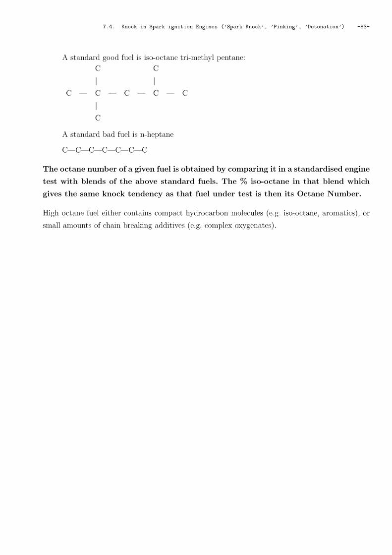
7.4. Knock in Spark ignition Engines (’Spark Knock’, ’Pinking’, ’Detonation’) -83-
A standard good fuel is iso-octane tri-methyl pentane:
C C
| |C — C — C — C — C
|C
A standard bad fuel is n-heptane
C—C—C—C—C—C—C
The octane number of a given fuel is obtained by comparing it in a standardised engine
test with blends of the above standard fuels. The % iso-octane in that blend which
gives the same knock tendency as that fuel under test is then its Octane Number.
High octane fuel either contains compact hydrocarbon molecules (e.g. iso-octane, aromatics), or
small amounts of chain breaking additives (e.g. complex oxygenates).

-84- Chapter 7. Spark ignition engines
Appendix of chapter 7
7.A Ideal cycle /real cycle comparison
Common conditions: compression ratio rv = 10
before compression: p1 = 1 bar, T1 = 300 K
after combustion: p3 = 100 bar, T3 = 3000 K
Results of ideal cycle predictions for Constant Volume (Otto cycle)
Working Fluid γc γexh T4 K p4 bar φ ηcy % pm bar
Ideal air 1.4 1.4 1194 4.0 - 60.4 12.5
Real air 1.384 1.295 1522 5.1 - 52.6 14.5
CH4/air* 1.362 1.250 1684 5.6 1.056 747.7 15.5
C8H18/air* 1.33 1.253 1676 75.9 1.014 48.5 16.7
Ideal/real comparison
Fuel-air cycle+ 1.33 1.253 1.0 45.9 15.6
Typical S.I. engine:
full load (indicated) 1.0 37 12.5
full load (brake) 1.0 30 10
* No dissociation, + including dissociation

Chapter 8. Spark ignition engines: combustion control -85-
Chapter 8: Spark ignition engines: combustion
control
(p 192 Stone, 1999, §4.6)
8.1 Throttle control
Since φ ≃ 1 is required for adequate combustion, control of load (pm) or torque requires that the
mass of air and fuel mixture be reduced below that for atmospheric density. Hence
a) Throttle control intake density.
b) At low load a significant loss occurs
– pressure drop across the throttle is irreversible
– negative pumping loop on p-V diagram.
8.2 Fuel Supply
Fuel supply must be arranged to give
a) φ ≃ 1 at all conditions
b) good distribution and evaporation of liquid.
The air/fuel mixture can be prepared by either a carburettor or a fuel injection system. In both
cases fuel will be present in the inlet manifold as vapour, liquid droplets and a liquid film. Al-
though emissions legislation is now reducing the scope for using carburettors (§8.2.1), their use is
still widespread.
There are two types of fuel injection system used on spark ignition engine, multi-point injection
(§8.2.3) and single-point injection (§8.2.2).
8.2.1 Carburettor
Carburettor relies on Venturi principle to meter fuel in proportion to air flow (see Stone, 1999,
figures 4.40 onwards). The carburetor has a narrowed throat (or Venturi) in which the speed of
the air entering the engine increases, causing the pressure to drop (pV < p0). The pressure drop

-86- Chapter 8. Spark ignition engines: combustion control
between this point and the atmosphere causes the fuel to flow from the float chamber of the car-
buretor into the air stream. The fuel entering the air stream enters as liquid droplets.
air
Venturi throat
fuel
p0
pv
throttlevalve
p0
float valve
float
chamber
Figure 8.1. Carburettor
The mass of fuel entering must be controlled so that it is proportional to the mass of air flowing
through the venturi. In addition, the droplet size must be controlled, the droplets must be encour-
aged to evaporate, the resulting vapour must be mixed uniformly with the air, and some source of
heat must be provided to prevent the cooling resulting from the droplet evaporation from causing
freezing of the water vapour in the air. In addition, provision must be made for modification of
the mixture in response to engine temperature and operation (warm-up, idle, cruise, full power or
acceleration).
The modern carburetor is a fairly sophisticated device, with many small passages and jets, de-
signed to meet all these needs under changing conditions. The carburetor can also be electronically
controlled.
However, the fuel vaporization and mixing in a carburetted engine is far from perfect even under
the best circumstances. Problems:
a) Uneven fuel distribution between cylinders: fuel delivered to the various cylinders is not
equal, some cylinders running a little rich and some a little lean. Typically, the mixture is
adjusted se that the leanest cylinder is rich enough to run reliably, which means that the
richest cylinder is probably putting considerable unburned hydrocarbons into the exhaust.
b) Effects of non steady flow
c) Balance of multi carburettor systems.
d) Load change is transient: Under acceleration, the additional fuel sprayed from the accelerator
jet is largely unevaporated.

8.3. Performance -87-
8.2.2 Injection system
A carburettor can be replaced by a fuel injection system. In fuel injection system the pressure of
the fuel is monitored this improves control (pressure differences up to 5-7 MPa). A better control
implies reduction of fuel consumption, reduction of pollution particularly unburned hydrocarbons
and oxides of nitrogen. Main system are
DI: direct injection system the fuel is directly injected in the cylinder,
IDI: indirect injection system, the fuel is injected before the injection valve
MPI: multipoint injection system there is fuel injection into the intake port of each cylinder
SPI: Single Point Injection system, there are much simpler than the multipoint injection system
but a single point injection does not solve either of the problems (a) or (d) of the carburettor.
8.2.3 Multi point injection (MPI)
Multi point injection (MPI) allows for electronic control and implies injection into the intake
port of each cylinder.
From Stone (1999)figure 4.50 page 201.
Figure 8.2. Electronic fuel injection system
8.3 Performance
Each engine has a characteristic constant speed performance, with minimum sfc at a different φ
for each throttle opening.

-88- Chapter 8. Spark ignition engines: combustion control
Figure 8.3. Spark engine performance
8.4 Combustion chamber design
The main considerations in combustion chamber design are:
(i) the distance travelled by the flame front should he minimised. By minimising the distance
between the spark plug and the end gas, combustion will be as rapid as possible. This has
two effects:
– Firstly, it produces high engine speeds and thus higher power output.
– Secondly, the rapid combustion reduces the time in which the chain reactions that lead
to knock can occur.
This implies that, for geometrically similar engines, those with the smallest diameter cylin-
ders will be able to use the highest compression ratios.
(ii) Good turbulence generation:
– Sufficient turbulence to promote rapid combustion.
– However, too much turbulence leads to excessive heat transfer from the chamber con-
tents and also to too rapid combustion, which is noisy.
The turbulence can be generated by squish areas or shrouded inlet valves.
(iii) The exhaust valve should be as close as possible to the sparking plug. The exhaust valve is
very hot (possibly incandescent) so it should be as far from the end gas as possible to avoid
inducing knock or pre-ignition.
(iv) The end gas should be in a cool part of the combustion chamber. The small clearance between
the cylinder head and piston in the squish area forms a cool region. Since the inlet valve is
cooled during the induction stroke, this too can be positioned in the end gas region.

8.5. Emissions -89-
Combustion chamber design must optimise flame travel, generates good turbulence, that is use
large valve area, small quench surface area. See some example in Stone (1999) figure 4.6, 4.10,
4.11, 4.13 Heywood (1988) figure 15.15 page 845.
8.5 Emissions
8.5.1 Combustion Kinetics
A flame represents a fast reaction, only limited by chemical equilibrium at high temperature. But
during expansion stroke there is a slow reduction of temperature during which the rate of reaction
is itself reduced, and becomes much slower than the rate of change of equilibrium composition.
Hence concentrations of dissociated products produced at high temperature (before expansion)
become frozen at levels associated with these high temperatures. e.g.
2NO N2 + O2
2CO + O2 2CO2
give high NO, CO
(From Heywood, 1988, page 594) figure 8.4 left Results or kinetic calculations of CO concentrations
Figure 8.4. Formation of dissociate product
during expansion stroke following in SI engine stoichiometric mixture. figure 8.4 right Predicted
CO concentration at end of expansion stroke, compared with measured exhaust concentrations,
as function of air/fuel ratio α.
8.5.2 Hydrocarbons (see Heywood Fig. 11-1)
(a) Incomplete combustion of end gas
(b) compression of HC into crevices and absorption in oil layers and deposits
(c) expansion and desorption of HC at low pressure

-90- Chapter 8. Spark ignition engines: combustion control
(d) piston scrapes HC off walls and pushes into exhaust.
8.5.3 Pollution of the Environment
a) NO, NO2, CO are directly toxic
b) NO contributes to acid rain
c) NOx with HC + sunlight → peroxyacetyl nitrates (brown fog e.g. Los Angeles or Athens)
8.5.4 Emissions control
a) Control of φ alone is insufficient since maximum NOx occurs at φ ≃ 0.9 (best s.f.c. !) (but
see b-ii below)
b) NOx can be reduced if maximum temperature reduced. Options are
i mix exhaust gas with intake air (Exhaust Gas Recirculation, EGR)
ii Very lean mixture (φ < 0.65), i.e. ’Lean Burn’ - very difficult to control
c) Catalyst in exhaust system,
oxidises CO,
oxidises HC
reduces NOx
simultaneously(3 way catalyst)
Figure 8.5. 3-way catalyst
As shown in figure 8.5, from Heywood (1988) page 656, this requires φ = 1.00 for efficient
operation. Hence usually combined with MPI and complex control system including λ sensor.
(See also Stone, 1999, pages 172-3)
8.6 Stratified charge
Stratified charge means that mixture in the combustion chamber is not homogeneous any more.
The combustion chamber contains a rich zone (φ ≤ 1) near the spark plug and a very lean zone
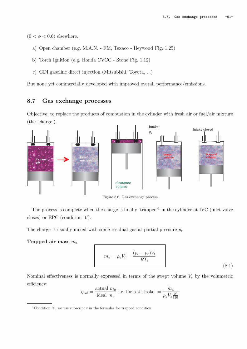
8.7. Gas exchange processes -91-
(0 < φ < 0.6) elsewhere.
a) Open chamber (e.g. M.A.N. - FM, Texaco - Heywood Fig. 1.25)
b) Torch Ignition (e.g. Honda CVCC - Stone Fig. 1.12)
c) GDI gasoline direct injection (Mitsubishi, Toyota, ...)
But none yet commercially developed with improved overall performance/emissions.
8.7 Gas exchange processes
Objective: to replace the products of combustion in the cylinder with fresh air or fuel/air mixture
(the ’charge’).
E x h a u s tg a sF r e s hm i x t u r e
c l e a r a n c e v o l u m e
s w e p tv o l u m et r a p p e dv o l u m e
I n t a k e c l o s e dI n t a k er a
Figure 8.6. Gas exchange process
The process is complete when the charge is finally ’trapped’1 in the cylinder at IVC (inlet valve
closes) or EPC (condition ’t’).
The charge is usually mixed with some residual gas at partial pressure pr
Trapped air mass ma
ma = ρaVt =(pt − pr)Vt
RTt
(8.1)
Nominal effectiveness is normally expressed in terms of the swept volume Vs by the volumetric
efficiency:
ηvol =actual ma
ideal ma
i.e. for a 4 stroke =ma
ρaVsN120
1Condition ’t’, we use subscript t in the formulas for trapped condition.

-92- Chapter 8. Spark ignition engines: combustion control
where ρa may be either of:
ρ0 of atmospheric air (for overall charging effect)
ρi in intake manifold (if throttled, ρi < ρ0 if supercharged, ρi > ρ0)
8.7.1 Sequence of events in four stroke cycle engines
blow down pc ≪ pe
exhaust expulsion
valve overlap:
a) throttled: pi < pe hence exhaust backflow (internal EGR)
b) supercharged or tuned: pi > pe hence charge through flow (scavenge) induction
backflow of charge into intake (if pc > pi before IVC)
8.8 Admission Valve
effective valve throat area Av
piston area Ap
vv
vp
p0
cylinder pressure p
IVCIVO
crank angle
Dp
Figure 8.7. Admission valve
At minimum pressure in the cylinder
1) Assuming incompressibility continuity requires
AvVv = ApVp
2) From Bernouilli equation we have
∆p =1
2ρVv
2
3) If the geometrical area at the valve is Ag and Av is the effective valve throat area, Av < Ag
we define a discharge coefficient CD such that
Av = CDAg
Typically, CD ≃ 0.6, 0.7 but depends on the definition of Ag

8.8. Admission Valve -93-
8.8.1 Exercise
In a 4-stroke engine cylinder with the inlet valve(s) fully open, typical maximum ratios of geometric
valve flow area to piston area are:
(a) 0.2 (single inlet valve)
(b) 0.26 (two inlet valves)
For a given engine with a stroke of 100 mm, the maximum piston speed is 1.62 times the mean
piston speed and a coefficient of discharge of 0.65 may be used for flow through the valves. If the
maximum instantaneous pressure drop across the inlet valves during the induction stroke is 0.2
bar, estimate the corresponding engine speed for each design. (Neglect compressibility effects for
this estimate and assume intake gas is air at 1 bar, 300 K)
Answers: (a) 4440, (b) 5770 rev.min−1

-94- Chapter 8. Spark ignition engines: combustion control
Appendix of chapter 8
8.A Diagram of an L-Jetronic system
Figure 8.8. Electronic multipoint port fuel injection system L-Jelectronic system
From Heywood (1988) figure 7-12 page 297.

8.8. European Vehicle Exhaust Emission Standards -95-
8.B European Vehicle Exhaust Emission Standards
Maximum pass levels from analysis of constant volume bag sample for duration of EU test drive
cycle passenger cars only Ail values n g.km−1
Spark ignition engines diesel engines (where different)
Year CO HC NOx
1971 14
1977 12 3.0
1979 10.5 2.5
HC + NOx
1984 10 5
1988 2
1993 2.72 0.97
1997 2 0.5
2000⋆ 2.3 0.2 0.15
2005⋆ 1 0.1 0.08
1997 1 DI 0.9 - IDI 0.7
2000⋆ 2.3 0.12 0.15
2005⋆ 1 0.1 0.08
* including cold start

-96- Chapter 8. Spark ignition engines: combustion control

Chapter 9. Combustion ignition engines: diesel engines -97-
Chapter 9: Combustion ignition engines: diesel
engines
9.1 Combustion
9.1.1 Fundamental features
In diesel engines, the spark plug is replaced by a fuel injector and only air is compress during the
compression process.
air -fuel mixture
air
fuel spray
spark plug fuel injector
pre
ssure
p
Q2-3
Q4-1
2 3
4
1
V2aV2
V2
rvV2 = V1
volume
Figure 9.1. Diesel cycle
In an ideal diesel cycle the processes are all reversible, and are as follows
1-2 isentropic compression of air through a volume ratio or
compression ratio
rv =V1
V2
2-3 addition of heat Q2−3 at constant pressure while the volume expands through
α the load or cut-off ratio
α =V3
V2
3-4 isentropic expansion of air to the original volume V1
4-1 rejection of heat Q4−1 at constant volume to complete the cycle
• Fuel is injected at the end of compression after point 2
• ignition results from a high air temperature
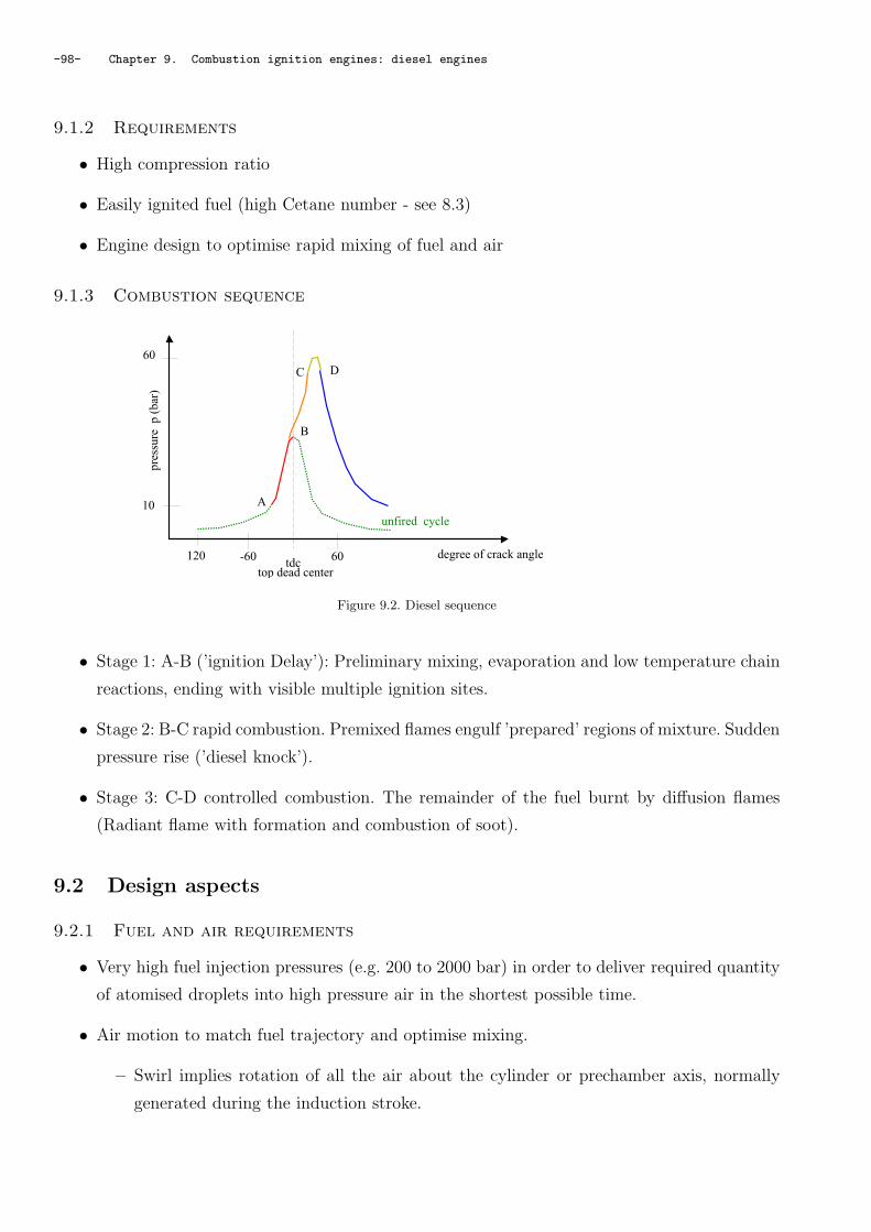
-98- Chapter 9. Combustion ignition engines: diesel engines
9.1.2 Requirements
• High compression ratio
• Easily ignited fuel (high Cetane number - see 8.3)
• Engine design to optimise rapid mixing of fuel and air
9.1.3 Combustion sequence
unfired cycle
degree of crack angle-60 60120 tdctop dead center
10
60
pre
ssure
p (
bar
)
A
B
C D
Figure 9.2. Diesel sequence
• Stage 1: A-B (’ignition Delay’): Preliminary mixing, evaporation and low temperature chain
reactions, ending with visible multiple ignition sites.
• Stage 2: B-C rapid combustion. Premixed flames engulf ’prepared’ regions of mixture. Sudden
pressure rise (’diesel knock’).
• Stage 3: C-D controlled combustion. The remainder of the fuel burnt by diffusion flames
(Radiant flame with formation and combustion of soot).
9.2 Design aspects
9.2.1 Fuel and air requirements
• Very high fuel injection pressures (e.g. 200 to 2000 bar) in order to deliver required quantity
of atomised droplets into high pressure air in the shortest possible time.
• Air motion to match fuel trajectory and optimise mixing.
– Swirl implies rotation of all the air about the cylinder or prechamber axis, normally
generated during the induction stroke.

9.2. Design aspects -99-
– Squish implies a squeezing effect between piston edge and cylinder head, resulting in
a lateral or radial airflow, and often a powerful toroidal vortex in which the swirl is
amplified by a reduction of radius with the same moment of momentum.
• Combustion chambers for smaller Direct Injection (D.I.) high speed engines may be designed
for wall wetting by the fuel, because impingement of the fuel jet on some part of the cylinder
wall cannot be prevented. This is commonly combined with both swirl and squish (Heywood,
1988, figure 10-1, page 494).
• Other small engines use Indirect Injection (I.D.I.) of the fuel into some form of prechamber
(Heywood, 1988, figure 10-2, page 495) which generally reduces noise but increases heat
loss and fuel consumption.
9.2.2 General
• Speed: Stage 1 of combustion is difficult to accelerate because chemical kinetics are not
affected by turbulence; the effect of high engine speed is therefore to create a large region
of evaporated fuel before ignition, and intensified ’Diesel knock’. This places a limit on the
maximum engine speed.
• Cylinder size: not limited by combustion (good for ship)
• Maximum load: usually limited by exhaust smoke (soot) (at least for naturally aspirated en-
gines) to a lower bmep than for spark ignition (i.e. overall φ < 1). Turbocharging can however
more than double the output without combustion limitations, giving high power/weight and
power/cost.
• Structure: High cylinder pressures and vibration sometimes require a heavier engine than
for SI.
• Cost: High pressure fuel injection requires very high precision components, which are the
major cost premium in small naturally aspirated engines.
9.2.3 Fuel Injection Systems
(e.g reference Stone, 1999, §5.5.2 page 234)
• Requirements:
– High pressure pump
– Precision injector: nozzles to match combustion system exact on/off control

-100- Chapter 9. Combustion ignition engines: diesel engines
– Control of injection timing and of volume injected.
• Hardware:
– Plunger pumps (1 per cylinder) ( with separate HP fuel pipes or Rotary distributor
pump) and injectors or Unit injectors operated directly from camshaft
– Governor or electronic control unit
• Normal Features:
– Spill port controls start and end of injection
– Spill timing by helical grooves in pump piston or solenoid control of spill port
– Pump delivery valve and injector pressure balance provide bi-stable injector switching
9.3 Fuel and cetane number
’Diesel’ or ’Derv’ is typically gasoil, i.e. a crude oil fraction of higher density and lower volatility
than gasoline.
The Cetane Number measures its quality in reducing diesel knock, i.e. in producing rapid ignition
(effectively the opposite requirement to that for a high octane fuel, and hence a long straight chain
compound is good).
Definition:
The cetane number of a fuel is the % n-cetane (C16H34) in a mixture of n-cetane with
α-methyl naphthalene (C11H10 double ring) which gives the same diesel knock effect
as the fuel under test.
In practice, α-methyl naphthalene is found to be insufficiently stable for standard tests, and
heptamethyl nonane (HMN, C16H34, CN=15) is used in ASTM method D6l3 such that CN= %
n-cetane +0.15× %HMN.
9.4 Emissions
9.4.1 Incomplete combustion products
• Soot (from diffusion flames) very sensitive to
– combustion design,
– injector maintenance

9.5. Spark ignition engines compared to compression ignition engines -101-
• HC, oxygenates, CO from decomposed fuel in fuel rich regions quenched lean flames.
For future standards, these components may need an oxidation reactor. (Also is some soot car-
cinogenic? Can micron sized particles harm the lungs?)
9.4.2 NOx production
NOx is formed locally wherever 0.7 > φ > 0.9 at high temperatures. It is generally regarded as
the most serious constituent since:
• 3 way catalyst is not applicable
• it is hard to reduce NOx in an oxidising atmosphere.
EGR and water injection can be used to reduce the temperature and hence formation rate.
Retarded injection timing also reduces maximum temperature
9.5 Spark ignition engines compared to compression ignition engines
9.5.1 Emissions
Generally less fundamentally serious for compression ignition than emissions from spark ignition
engines due to
• overall lean mixture
• low sensitivity to engine temperature on start up
9.5.2 Naturally Aspirated Engines: effect of overall fuel/air ratio
57
9b m p e ( b a r )
f0 . 5 1 1 . 2
C I
S I
Figure 9.3. CI and SI φ regimes

-102- Chapter 9. Combustion ignition engines: diesel engines
9.5.3 Typical parameters
spark ignition compression ignition
Max. cylinder bore, mm 150 1000
Compression Ratio 8-12 12 - 24
Max. bmep, bar 10 8 (N.A.)
10-20 (T/C)
Max. cylinder pressure, bar 50 100
Max. Rev/min 5000- 15000 5000
Load control Throttle Fuel volume only
Emissions CO,NOx,HC NOx , HC, particulates
9.5.4 Fuel consumption
Figure 9.4. Comparison of the part load efficiency 0f engines at 2000 rpm (Stone, R.) spark ignition and Diesel

Chapter 10. Two stroke cycle engines -103-
Chapter 10: Two stroke cycle engines
(p 320 Stone, 1999, ch 7)
10.1 Sequence of events
Figure 10.1. Two stroke piston engine - scavenging
With reference to figure 10.1 the following processes occur in a two-stroke engine, at times
determined by the piston covering and uncovering ports in the cylinder wall:
1 At about 60 before bottom dead centre the piston uncovers the exhaust port and exhaust
blowdown occurs, such that the cylinder pressure approaches the ambient pressure. This is
the end of the power stroke.
2) Some 5-l0 later the inlet port is opened and the charge compressed by the underside of the
piston in the crankcase is able to flow into the cylinder. With this loop scavenge arrangement
(figure c), the incoming charge displaces and mixes with the exhaust gas residuals; some
incoming charge will flow directly into the exhaust system.
3) The scavenge process ends with both the crankcase and cylinder pressure close to the ambient
pressure level once the inlet port is closed (about 55 after bottom dead centre). Towards
the end of the scavenge process, there can be a backflow of charge and exhaust gas residuals
into the crankcase. The upward movement of the piston now reduces the pressure in the
crankcase.
4) At about 60 after bottom dead centre the exhaust port is closed, and the charge is com-
pressed by the upward motion of the piston.

-104- Chapter 10. Two stroke cycle engines
5) 5 At about 60 before top dead centre the pressure in the crankcase is significantly below
the ambient pressure, and the crankcase port opens to allow the incoming charge to flow
lino the crankcase.
6) Ignition occurs typically within the range of 10-40 before top dead centre. Work is done
by the engine on the gas until top dead centre, at which point the power stroke starts, and
continues until the exhaust port opens.
7) The crankcase port is closed at about 60 after top dead centre, but prior to this there will
he some outflow of gas from the crankcase, as the crankcase pressure will have risen above
the ambient pressure level around top dead centre.
Two undesirable features of the two-stroke engine are
• the mixing of the incoming charge with the exhaust residuals,
• and the passage of the charge direct mo the exhaust system.
The fuel loss due to these shortcomings is largely eliminated in diesel engines (not considered
here are model diesel engines), as they are invariably supercharged and there is in-cylinder fuel
injection.
10.2 Design Options
Sequence of events:
blow down pcharge ≫ pexhaust (and pcharge ≫ pscavenge)
scavenge pscavenge > pexhaust requires scavenge pump / blower
Scavenge system: Uniflow, Loop or cross flow Ports and/or valves Crankcase, under piston, or
separate pump
Exhaust tuning
Supercharge (requires increased exhaust pressure)
10.3 Scavenge process
As some air has leaked to through the exhaust ma 6= ms.
10.3.1 Dimensionless performance parameters
In order to discuss the gas exchange performance of two-stroke engines, it is necessary to define
several gas flow parameters.

10.3. Scavenge process -105-
Vt
exhaust
air supplydensity rs
Definition:
vt : cylinder trapping volumemi : ideal trapped air mass = ρsVt
ma : actual air mass in the cylindermg : mass of residual gas in the cylinderms : mass of air supplied to the cylinder
Figure 10.2. Scavenge process in a two stroke engine
Scavenge ratio or delivery ratio λ
λ =ms
mi
(10.1)
Scavenge efficiency ηsc
ηsc =ma
ma + mg
(10.2)
Charging efficiency ηch
ηch =ma
mi
(10.3)
Trapping efficiency ηtr
ηtr =ma
ms=
ηch
λ(10.4)
There is a special case if we assume p and T to be constant throughout:
ma + mg = mi
and
ηsc = ηch
but in practice, Tg > Ts, ρg < ρs, ma + mg < mi and ηsc > ηch
10.3.2 Perfect displacement model
In this model exhaust products are displaced by fresh mixture without mixing
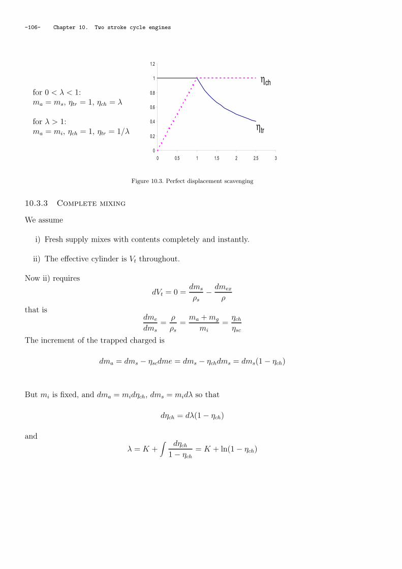
-106- Chapter 10. Two stroke cycle engines
for 0 < λ < 1:ma = ms, ηtr = 1, ηch = λ
for λ > 1:ma = mi, ηch = 1, ηtr = 1/λ
0
0.2
0.4
0.6
0.8
1
1.2
0 0.5 1 1.5 2 2.5 3
htr
hch
Figure 10.3. Perfect displacement scavenging
10.3.3 Complete mixing
We assume
i) Fresh supply mixes with contents completely and instantly.
ii) The effective cylinder is Vt throughout.
Now ii) requires
dVt = 0 =dms
ρs
− dmex
ρ
that isdme
dms=
ρ
ρs=
ma + mg
mi=
ηch
ηsc
The increment of the trapped charged is
dma = dms − ηscdme = dms − ηchdms = dms(1 − ηch)
But mi is fixed, and dma = midηch, dms = midλ so that
dηch = dλ(1 − ηch)
and
λ = K +∫
dηch
1 − ηch= K + ln(1 − ηch)

10.3. Scavenge process -107-
0
0.2
0.4
0.6
0.8
1
1.2
0 0.5 1 1.5 2 2.5
hch=1-e-l
htr=(1-e-l)/l
Figure 10.4. Complete mixing scavenging, as a function of λ
10.3.4 Short Circuit Flow
Each increment of fresh charge supplied is immediately discharged to exhaust. Hence for all dms
and all λ:
hch
l
dηch = 0 = dηtr
Figure 10.5. Short circuit scavenging
10.3.5 Combined Scavenge Model
Models 10.3.2, 10.3.3 and 10.3.4 may be combined in any desired manner e.g. suppose initial
scavenge a is by displacement, followed by a combination b of displacement, mixing and short
circuit as in figure 10.6.
Then total
dηch = δdλ + µ(1 − ηch)δdλ
hence
dλ =dηch
δ + µ(1 − ηch)
and
λ − λI =∫ ηch
λI
dηch
δ + µ(1 − ηch)= −1
µln
[δ + µ(1 − ηch)
δ + µ(1 − λI)
]
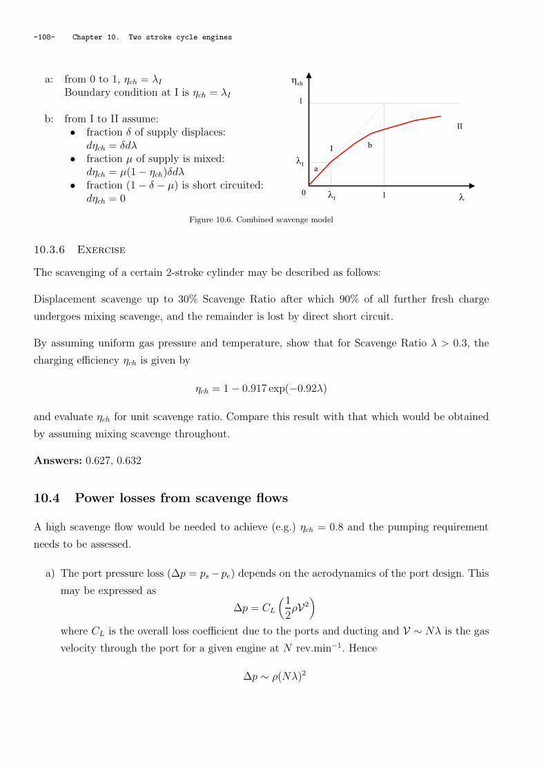
-108- Chapter 10. Two stroke cycle engines
a: from 0 to 1, ηch = λI
Boundary condition at I is ηch = λI
b: from I to II assume:• fraction δ of supply displaces:
dηch = δdλ• fraction µ of supply is mixed:
dηch = µ(1 − ηch)δdλ• fraction (1 − δ − µ) is short circuited:
dηch = 0
hch
l
I
II
a
b
1
1lI
lI
0
Figure 10.6. Combined scavenge model
10.3.6 Exercise
The scavenging of a certain 2-stroke cylinder may be described as follows:
Displacement scavenge up to 30% Scavenge Ratio after which 90% of all further fresh charge
undergoes mixing scavenge, and the remainder is lost by direct short circuit.
By assuming uniform gas pressure and temperature, show that for Scavenge Ratio λ > 0.3, the
charging efficiency ηch is given by
ηch = 1 − 0.917 exp(−0.92λ)
and evaluate ηch for unit scavenge ratio. Compare this result with that which would be obtained
by assuming mixing scavenge throughout.
Answers: 0.627, 0.632
10.4 Power losses from scavenge flows
A high scavenge flow would be needed to achieve (e.g.) ηch = 0.8 and the pumping requirement
needs to be assessed.
a) The port pressure loss (∆p = ps −pe) depends on the aerodynamics of the port design. This
may be expressed as
∆p = CL
(1
2ρV2
)
where CL is the overall loss coefficient due to the ports and ducting and V ∼ Nλ is the gas
velocity through the port for a given engine at N rev.min−1. Hence
∆p ∼ ρ(Nλ)2

10.5. Comparison with four stroke engines -109-
b) Power consumption: from SFEE
−Wrev =∫ e
sV dp ≃ V ∆p
if ∆p is small and hence since
V ∼ Nλ
also
−Wrev ≃ ρ(Nλ)3 (10.5)
or for a real scavenge pump with isentropic efficiency ηc:
Wsc ∼ρ(Nλ)3
ηc
10.4.1 Exercise
For the engine of exercise 10.3.6, the total pressure drop ∆p across the cylinder ports is found to
be 0.25 bar when λ = 1.0. The fresh charge is supplied by a mechanically driven compressor of
isentropic efficiency 0.85.
(a) What is the compressor work loss when expressed as a loss of mean effective pressure of the
engine? (Assume that cylinder trapping volume = swept volume).
(b) The engine power is to be raised by increasing the scavenge flow until ηch = 0.8. Find the
required value of λ and estimate the new work loss involved.
Assume compressibility may be neglected, so that ∆p ∼ λ2 and density changes are ignored. Is
this assumption justified by your result?
Answers: (a) 0.29 bar, (b) 1.69, 1.4 bar
10.5 Comparison with four stroke engines
The absence of the separate induction and exhaust in the two-stroke engine is the fundamental
difference from four-stroke engines. In two-stroke engines, the gas exchange or scavenging processes
can the induction and exhaust occurring simultaneously. Consequently the gas exchange processes
in a two-stroke engine are much more complex than in four-strokes engines, and the gas exchange
is probably the most important factor controlling the efficiency and performance of two-stroke
engines.
Two-stroke engines can be either spark ignition or compression ignition, and currently the largest
and smallest internal combustion engines utilise two-stroke operation. The smallest engines are
those used in models, for which compression ignition (perhaps assisted by a glow plug for starting)

-110- Chapter 10. Two stroke cycle engines
is more common than spark ignition. The output of these engines is frequently much less than 100
W. Small two-stroke engines with outputs in the range of approximately 1-100 kW are usually
naturally aspirated with spark ignition. The typical applications are where low mass, small bulk
and high-power output are the prime considerations - for example motor cycles, outboard motors,
chain saws, small generators etc.
4 stroke 2 stroke
Fuelling port injection cylinder injection
Evaporation heated port wall air blast spray
Overall φ φ = 1. φ < 1 (air through flow) lean
Max bmep (pbm) 10 bar 6 bar ?
NOx control 3 way cat. + EGR internal EGR
HC control 3 way cat. oxidation cat.

Revision questionnaire of Part II -111-
Revision questionnaire of Part II
1) What are swept volume and volumetric efficiency in a piston engine?
2) What are mean effective pressure, brake mean effective pressure and indicated mean effective
pressure, friction mean effective pressure?
3) When are two-stroke engines to be used?
4) Explain the difference between spark ignition engine and compression ignition engine.
5) What are direct and indirect injection in the context of piston engines?
6) Explain the difference between carburettor single point injection and multipoint injection.
7) What is the interest of stratified charges?
8) Give the main criteria for combustion chamber design.
9) Plot Otto and diesel p-V diagrams.
10) What is knock in spark engine and how can it be prevented?
11) What are the 1st stage and 2nd stage of combustion in a spark engine and how are they
defined?
12) What is the difference between swept and trapped volume?

-112- Revision questionnaire of Part II

part III: Supercharging and Turbocharging -113-
Part III
Supercharging and Turbocharging

-114- part III: Supercharging and Turbocharging

Chapter 11. Supercharging and turbocharging -115-
Chapter 11: Supercharging and turbocharging
Breathing exercises (Stone, 1999, ch 9), (Lumley, 1999, 2.14)
11.1 Purpose
Engine power can be increased if more air can be trapped in the cylinder by raising the pressure
and hence the density ρa of the air.
An engine is supercharged or turbocharged if the mean pressure at the intake port
is higher than ambient.
11.1.1 supercharger
Supercharging used to be the generic term for using some mechanical device for increasing the
inlet density; now
Supercharger refers to mechanically driven compressor; it is take to refer only to positive
displacement devices.
compressorturbine
inlet air
Wengine
exhaustgas
compressor
inlet air
Wengine
exhaustgas
Figure 11.1. Supercharging (left) and turbocharging (right)
In a positive displacement device there is no direct connection between inlet and outlet; air is taken
into a chamber, which is then closed. The volume of the chamber may be reduced, increasing the
pressure, and the chamber is then opened to the outlet that is the engine inlet as in figure 11.1
left.
Roots shown in figure 11.2 are positive displacement machines. The rotors in the roots are not
in contact, but are held in the proper relative position, and are rotated, by gears outside the
compressor casing. Notice that the air trapped between the rotors in the Roots is not compressed

-116- Chapter 11. Supercharging and turbocharging
(since the volume of the space does not change), until it is delivered to the receiver at the outlet,
when it is compressed by the backflow of the higher pressure air in the receiver. For this reason,
the efficiency of the Roots is a little lower than that of other types. The vanes in the Judson, on
the other hand, slide in and out, changing the volume of the spaces as they carry the air around
from inlet to outlet.
Figure 11.2. Examples of superchargers, Roots blower, vane compressor, screw compressor
11.1.2 Turbochargers
In a turbocharger the exhaust turbine is driven by the compressor see figure 11.3.
air inlet
compressor turbine
exhaust gas
inlet manifold
(charge air cooler)
exhaust manifold
WtWc
ma, p0, T0
pe, Te
pa, Ta
me, p0, Te0
fuel
inje
ctor
Figure 11.3. Schematic of turbocharged engine system
Turbocharging is used to refer to dynamic device. A dynamic device is one, like a centrifugal
compressor, in which there is a direct connection between the inlet and the outlet (so that, if the
device were not rotating, there would be no pressure difference), and which produces its pressure
difference from the motion of winglets, or blades, through the air, produced by rotation of the
device.
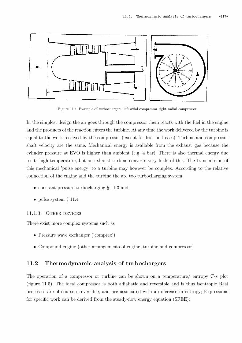
11.2. Thermodynamic analysis of turbochargers -117-
Figure 11.4. Example of turbochargers, left axial compressor right radial compressor
In the simplest design the air goes through the compressor them reacts with the fuel in the engine
and the products of the reaction enters the turbine. At any time the work delivered by the turbine is
equal to the work received by the compressor (except for friction losses). Turbine and compressor
shaft velocity are the same. Mechanical energy is available from the exhaust gas because the
cylinder pressure at EVO is higher than ambient (e.g. 4 bar). There is also thermal energy due
to its high temperature, but an exhaust turbine converts very little of this. The transmission of
this mechanical ’pulse energy’ to a turbine may however be complex. According to the relative
connection of the engine and the turbine the are too turbocharging system
• constant pressure turbocharging § 11.3 and
• pulse system § 11.4
11.1.3 Other devices
There exist more complex systems such as
• Pressure wave exchanger (’comprex’)
• Compound engine (other arrangements of engine, turbine and compressor)
11.2 Thermodynamic analysis of turbochargers
The operation of a compressor or turbine can be shown on a temperature/ entropy T -s plot
(figure 11.5). The ideal compressor is both adiabatic and reversible and is thus isentropic Real
processes are of course irreversible, and are associated with an increase in entropy; Expressions
for specific work can be derived from the steady-flow energy equation (SFEE):

-118- Chapter 11. Supercharging and turbocharging
for an adiabatic turbine (wt > 0)
wt = hin − hout = h3 − h4 (11.1)
and for an adiabatic compressor (wc < 0)
wc = hin − hout = h1 − h2 (11.2)
For real gases, enthalpy is a strong function of temperature and a weak function of pressure. For
enth
alpy h
entropy S
2s
1
DWc
p2 : compressor outlet
p0 : ambiant pressure
2
p3 : turbine inlet
4s4
DWt
3
Figure 11.5. Enthalpy as a function of entropy diagram for a turbocharger
semi-perfect gases, enthalpy is solely a function of temperature, and this is sufficiently accurate
for most purposes. Thus
wc = cp(T2 − T1)
and
wt = cp(T3 − T4)
where cp is an appropriate mean value of the specific heat capacity. Consequently the T -s plot
gives a direct indication of the relative compressor and turbine works. This leads to isentropic
efficiencies that compare the actual work with the ideal work:
compressor isentropic efficiency:
ηc =h2s − h1
h2 − h1=
T2s − T1
T2 − T1(11.3)
and turbine isentropic efficiency,
ηt =h3 − h4
h3 − h4s=
T3 − T4
T3 − T4s(11.4)
It may appear unrealistic to treat an uninsulated turbine that is incandescent as being adiabatic.
However, the heat transferred will still be small compared to the energy flow through the turbine.
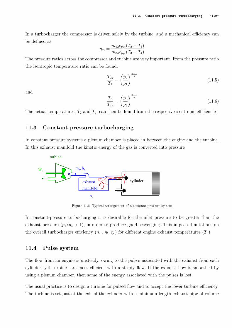
11.3. Constant pressure turbocharging -119-
In a turbocharger the compressor is driven solely by the turbine, and a mechanical efficiency can
be defined as
ηm =m12cp12
(T2 − T1)
m34cp34(T3 − T4)
The pressure ratios across the compressor and turbine are very important. From the pressure ratio
the isentropic temperature ratio can be found:
T2s
T1=
(p2
p1
) γ−1
γ
(11.5)
and
T3
T4s=
(p3
p4
) γ−1
γ
(11.6)
The actual temperatures, T2 and T4, can then be found from the respective isentropic efficiencies.
11.3 Constant pressure turbocharging
In constant pressure systems a plenum chamber is placed in between the engine and the turbine.
In this exhaust manifold the kinetic energy of the gas is converted into pressure
cylinderexhaust
manifold
turbine
pe
me, heWt
Figure 11.6. Typical arrangement of a constant pressure system
In constant-pressure turbocharging it is desirable for the inlet pressure to be greater than the
exhaust pressure (p2/p3 > 1), in order to produce good scavenging. This imposes limitations on
the overall turbocharger efficiency (ηm, ηt, ηc) for different engine exhaust temperatures (T3).
11.4 Pulse system
The flow from an engine is unsteady, owing to the pulses associated with the exhaust from each
cylinder, yet turbines are most efficient with a steady flow. If the exhaust flow is smoothed by
using a plenum chamber, then some of the energy associated with the pulses is lost.
The usual practice is to design a turbine for pulsed flow and to accept the lower turbine efficiency.
The turbine is set just at the exit of the cylinder with a minimum length exhaust pipe of volume

-120- Chapter 11. Supercharging and turbocharging
air inlet
compressor turbine
exhaust gas
Wc
ma, p0, T0
pe, Tepa, Ta
me, p0, Te0
Wt
fuel mfengine
Typical arrangement of a turbocharged engineoperating with the constant pressure system.The compressor and the turbine form aself-contained unit: the turbocharger
Figure 11.7. Constant pressure system for several cylinders
cylinder
turbine
Wt
Figure 11.8. Typical arrangement for pulse system
V0. The Exhaust valve opens suddenly and pressure rise instantaneously at the turbine inlet, the
burnt gases expand in the turbine providing some work Wt, this is the pulse. The higher V0/Vs
the higher the pressure rise at the turbine inlet and the higher Wt
However, if the compressor pressure ratio is above 3:1 the pressure drop across the turbine becomes
excessive for a single stage. For four-stroke engines no more than three cylinders should feed the
same turbine inlet. Otherwise there will be interactions between cylinders exhausting at the same
time.
For a four-cylinder or six-cylinder engine a turbine with two inlets should be used. The exhaust
connections should be such as to evenly space the exhaust pulses. Figure 11.10 shows a typical
arrangement of a turbocharged engine operating with the pulse system for a four cylinder engine.
A more realistic approach is to use pulse converters to connect groups of cylinders that would
otherwise be separate. For example, four cylinders could he connected to a single turbocharger
entry, (figure 9.14 Stone, 1999). The steadier flow can also lead to an improvement in turbine
performance. The design of the pulse converter is a compromise between pressure loss and un-
wanted pulse propagation. Reducing the throat area increases the pressure loss, but reduces the
pulse propagation From one group of cylinders to another. The optimum design will depend on

11.5. Energy available -121-
exhaust valve opened
bottom cylinder
maximum
pressure p0
pre
ssure
top cylinder
time t
maximumpressure pmax
real pulse
idealpulse
Figure 11.9. Pulse generation
Typical arrangement of a turbocharged engine operating with the pulse system.
Figure 11.10. Two-entry turbine inlet casing
the turbine, the exhaust pipe length, the valve timing, the number of cylinders, the engine speed
etc.
Constant-pressure turbocharging (that is, when all exhaust ports enter a chamber at approxi-
mately constant pressure) is best for systems with a high pressure ratio. The dissipation of the
pulse energy is offset by the improved turbine efficiency. Furthermore, during blown-down the
throttling loss at the exhaust valve will be reduced. However, the part load performance of a
constant-pressure system is poor because of the increased piston pumping work, and the positive
pressure in the exhaust system can interfere with scavenging.
11.5 Energy available
Analyses (see below) show that the ideal power output is the same for
a) complete expansion in the cylinder (§11.5.1)
b) an Ideal Pulse Turbine (§11.5.2) but may be smaller from

-122- Chapter 11. Supercharging and turbocharging
c) a Constant Pressure Turbine (§11.5.3) because of irreversible losses at the exhaust valve, in
this case there is a higher pressure in the cylinder throughout the exhaust stroke, which has
two effects:
– Work done on the gas by the piston benefits the turbine
– Scavenge flow is inhibited during valve overlap.
11.5.1 Expansion energy available at exhaust release point
(From R. Saunders)
Suppose that a full isentropic expansion is possible between 4 and atmospheric condition 5 (e.g.
extended stroke Atkinson cycle).
clearance volume Vc
swept volume Vs
volume V
1 - 6
2
3
4pres
sure
p
5p0
Otto Cycle
isentropic expansion
(pVg = cst)
p4 to po
Figure 11.11. Expansion energy available
Additional work obtained would be:
Wmax =∫ 5
4pdV +
∫ 6
5pdV
that is for an isentropic expansion
Wmax =p4V4 − p5V5
γ − 1
or using p5 = p0 and V6 = V4
Wmax = p0V4
[1
γ − 1
(p4
p0
)− γ
γ − 1
(V5
V4
)+ 1
]
but also V4 = rr−1
V5 and(
V5
V4
)=(
p4
p0
)1/γand
Wmax = p0V4
1 +
1
γ − 1
(p4
p0
)− γ
γ − 1
(p4
p0
) 1
γ

11.5. Energy available -123-
0
0.5
1
1.5
2
2.5
3
3.5
4
4.5
5
1 2 3 4 5 6 7
Figure 11.12. Maximump′
em
p0as a function of p4
p0available from exhaust gases, with r ≫ 1
and if expressed in terms of equivalent mean effective pressure the maximum additional p′em is
p′em =W ′
max
Vs=
r
r − 1p0
1 +
1
γ − 1
(p4
p0
)− γ
γ − 1
(p4
p0
) 1
γ
(11.7)
Hence
i) Substantial work potential from exhaust.
ii) Reverse of process 4-5-6 would be supercharging and the same analysis could be used.
iii) But typically, if p4
p0= 4, p′em
pem= 0.16 while v5
v6= 2.8.
11.5.2 Energy available from an adiabatic exhaust turbine: ideal pulse turbine
turbine
Wt
p0
he
p0
pre
ssure
4
6volume
Vs
Figure 11.13. Expansion energy available
We will assume an isentropic expansion between 4 and 6. Here we are dealing with an unsteady
flow process (see Cengel & Boles, 1998, §4.4 page 220). We will assume a uniform flow process
with a stationary piston so that he = h6 and T6
T4=(
p0
p4
) γ−1
γ .

-124- Chapter 11. Supercharging and turbocharging
The energy equation for non-steady flows ((Cengel & Boles, 1998, 4-35) yields
Q + Wt − mehe = U6 − U4
and mass conservation mass of gas: the mass of gas leaving the turbine me is equal to the mass
lost in the cylinder during the expansion m4 − m6
me = m4 − m6 =p4V4
RT4
− p6V6
RT6
=V4
R
(p4
T4
− p0
T6
)
and
mehe = mecpT6 =γ
γ − 1V4
p4
(p0
p4
) γ−1
γ
− p0
Also
U6 − U4 =p6V6 − p4V4
γ − 1=
V4
γ − 1(p0 − p4)
Hence additional available mep is
p′em =|Wt|Vs
=U4 − U6 − mehe
Vs=
V4
V5
p4 − p0
γ − 1− γ
γ − 1
(p0
p4
) γ−1
γ
− p0
p′em =|Wt|Vs
=r
r − 1p0
1 +
1
γ − 1
p4
p0− γ
γ − 1
(p4
p0
) 1
γ
11.5.3 Energy available from an adiabatic exhaust turbine: Constant pressure
exhaust manifold (4 stroke)
exhaust
manifold
turbine
pe
me, heWt
pe
p0
48
7
9
Figure 11.14. Energy available from a constant pressure exhaust manifold
• Energy equation for full EVO period: (boundary )
Q − W − mehe = U8 − U4

11.5. Energy available -125-
where
W = −peVs
he is averaged for exhaust
Ue is unchanged from 8 to 4
hence
mehe = peVs +p4V4 − peVc
γ − 1
• SFEE for the turbine only:
WT = me(he − h9) = mehe
(1 − h9
he
)
and if isentropic,
h9
he=
T9
Te=
(po
pe
)γ−1
γ
• Now net work is Wt − Vs(pe − po) for turbine + piston together full exhaust process. Hence
p′em =Wnet
Vs=
(pe +
rr−1
p4 − 1r−1
pe
γ − 1
)1 −
(po
pe
)γ−1
γ
− (pe − p0)
0
0.5
1
1.5
2
2.5
3
3.5
4
0 2 4 6 8 10 12 14 16 18 20
Figure 11.15. Maximum p′
em as a function of pe for a constant pressure manifold, with p4 = 4 bar and r ≫ 1

-126- Chapter 11. Supercharging and turbocharging

Chapter 12. Turbocharging design and modelling -127-
Chapter 12: Turbocharging design and modelling
12.1 Design analysis
In principle there is a choice between
• constant pressure system
• pulse system
In practice a proper analysis of the pulse system for the purpose of turbocharger matching is too
complex, and a ’quasi-steady’ method is used. For this purpose,
a) the effective exhaust pressure pe cannot be measured because of pulsation, but since it
depends on the flow capacity of the turbine it can be obtained from a turbine characteristic
map, for a given actual mass flow rate of gas.
b) The effective exhaust temperature Te depends on processes in the engine cylinder. Two
possible techniques are:
i) Simulate the full engine cycle including combustion to get the release temperature at
EVO, and use section 12.3
ii) Use an empirical method for gas temperature rise across the cylinder, based on exper-
imental data for a given engine (section 12.4 and below).
12.2 Turbocharger power balance
air inlet
compressor turbine
exhaust gas
Wc
ma, p0, T0
pe, Tepa, Ta
me, p0, Te0
Wt
fuel mfengine
Figure 12.1. Turbocharger

-128- Chapter 12. Turbocharging design and modelling
1. The condition for a stable operation that is a constant turbine and compressor speed is
Wt = Wc
2. For a real turbine
Wt = ηtme(he − he0s) = ηtmecpeTe
1 −
(p0
pe
) γe−1
γe
NB
a) Te depends on engine processes
b) pe depends on turbine and me
c) ηt depends on turbine, me, Ntc, pulse factor PF. e.g. we get pe and ηts from a steady
flow turbine test and use
ηt = PF.ηts
where PF is an empirical factor called the pulse factor taking into account the pulse
effect.
3. For a real compressor
Wc =ma
ηc
(hac − h0)
that is
Wc =ma
ηc
cpaT0
(
pa
p0
) γa−1
γa
− 1
ηc depends on compressor, ma, pa/p0
4. me = ma + mf and ma = ηtrms we can also introduce f the mass ratio of fuel to air f =mf
ms,
hence:
me = ma(1 + fηtr)
For diesel, me = ma may be an adequate approximation otherwise typical values may be
f ≤ 0.4 and ηtr ≤ 0.9.

12.3. Mean Temperature Te from known cylinder release conditions -129-
12.3 Mean Temperature Te from known cylinder release conditions
Energy: 1st Law for non-steady exhaust stroke:
Q − W − mehe = U8 − U4
with W = −peVs Hence
mehe = m4u4 − m8u8 + peVs
Mass conservation:
me = m4 − m8
So that
he = cpTe =cv
(T4 − m8
m4T8
)+ peVs
m4
1 − m8
m4
If the compression ratio is reasonably high, the effect of m8/m4 becomes small, and m4 ≃ p4Vs
RT4
HenceTe
T4
≃ 1
γ
(1 + (γ − 1)
pe
p4
)
Typical example: p4 = 4 bar, T4 = 800C = 1073 K, pe = 1.8 bar and γ = 1.35 would give
Te = 0.857 T4 = 920K = 647C
Figure 12.2. FIG. 10.11. Engine temperature rise factor K.
12.4 Empirical relationship for Te
From SFEE for engine, fuel energy is
mfLCV = WE + QC + mecpe(Te − Ta)
mecpe(Te − Ta)
mf × LCV= 1 − ηth − LC

-130- Chapter 12. Turbocharging design and modelling
me, pe, Tema, pa, Ta
fuel mfengine
NE rev/minWE
QE
Figure 12.3. SFEE in the turbocharged engine
where ηth = WE
mf×LCVand LC = QC
mf×LCVboth of which depend mainly on f and NE for a given
engine Now,me
mf=
ma + mf
mf= α + 1 =
1
fηtr+ 1
So
Te − Ta =LCV
cpe(1 − ηth − LC)
(1
α + 1
)=
K
α + 1
where K = K(f, NE) is an empirical factor for a given engine.
12.5 Example for a good diesel
ηth = 0.38, LC = 0.25, LCV = 42800 kJ.kg−1, cpe = 1.15 kJ.kg−1.K−1 would give
Te − Ta =13800
α + 1
(approx valid when α > 18)
when turbocharged, suppose pa = 2 bar is required when α = 24, p0 = 1 bar, T0 = 25C, ηc = 0.75
Then the compressor gives
Ta = T0
1 +2
2
7 − 1
0.75
= 298 × 1.292 = 385 K
and so
Te = Ta +13800
25= 937 K
Power balance requires
ηT mecpeTe
1 −
(p0
pe
) γe−1
γe
= cpa(Ta − T0)ma
If ηT = 0.7 and γe = 4/3, then pe
p0= 1.60

12.6. Exercise -131-
12.6 Exercise
For a certain design of 4-stroke engine operating at a given overall air/fuel ratio, it is found that
the i.m.e.p. and cylinder release pressure and temperature are each respectively proportional to
the density, pressure and temperature of the air in the inlet manifold. A test of such an engine
shows 10 bar i.m.e.p. and cylinder release conditions of 3.5 bar, 800C when the inlet conditions
are 1 bar, 30C.
(a) Find the equivalent i.m.e.p. and release conditions (turbine inlet and outlet) for the same
air/fuel ratio when the engine is fitted with a turbocharger which compresses the air to 1.8
bar at cylinder inlet, and bas an isentropic efficiency of 70% in both compressor and turbine.
(b) Hence by assuming a constant pressure exhaust system, find the exhaust manifold pressure
for steady conditions.
Neglect any flow of air through the engine as a result of valve overlap. Use γ = 1.4 for air, 1.333
for exhaust, and assume R is the same for both.
Answers: a) 14.28 bar, pe = 6.3 bar, 1080C, b) 1.35 bar
12.7 Exercise
For a certain turbocharged diesel engine, the averaged temperature rise from air manifold to
exhaust gas manifold is given by
∆T =12000
1 + A/F
(T in C) for A/F ≥ 18 where A/F is the total mass ratio of air to fuel flow.
(a) At a given load point at ambient conditions of 1 bar, 20C, the A/F is 20 and the compres-
sor delivers a boost pressure of 1.6 bar absolute with an isentropic efficiency (ηc) of 75%.
Calculate the average turbine gas inlet temperature and the corresponding pressure required
if the turbine isentropic efficiency (ηT ) and Pulse Factor (PF) are assumed to be 65% and
1.2 respectively. Use γ = 1.4 for air, 4/3 for exhaust gas.
(b) The same engine is also required to work at an altitude where the ambient conditions are
0.8 bar, 20C. The fuel input mass and boost pressure (absolute) at the given load point are
unchanged, but now ηc = 0.70, ηT = 0.60 and PF = 1.0. Calculate the new A/F and turbine
inlet conditions, by assuming that air mass flow is proportional to compressed air density.
Answers: a) 921 K, 1.31 bar, b) 18.14, 1012 K, 1.366 bar

-132- Chapter 12. Turbocharging design and modelling

Chapter 13. Elements of turbomachinery -133-
Chapter 13: Elements of turbomachinery
13.1 Dimensional analysis of compressible flows through
turbomachines
For a given design, the essential variables from an external point of view may be written as
p1, p2, RT1, RT2, m, N , D
where p and T are stagnation values
Note that
1) RT has dimension L2.t−2 (t = time)
2) Fixed gas composition is assumed (e.g. air)
3) Viscosity is omitted since the Reynolds number Re is assumed large (this is implied by
compressible flow).
Only 3 fundamental dimensions are required L, t, M. Hence we expect 7 − 3 = 4 independent
groups:
π1 π2 π3 π4
p2
p1
T2
T1
m√
RT1
D2p1
ND√RT1
Notes:
1) ηc, ηT = f(π2, π1) e.g. ηc =
(p2
p1
) γ−1
γ−1
T2
T1−1
2) π3 ∼ mρA
. 1√γRT1
∼ ca1
(where ca
is the flow Mach number) but in practice graphs use
m√
T
p
which is a dimensional mass flow parameter.
3) Similarly π4 ∼ umax
a1is a rotor Mach number but in practice graphs use
N√T
which is used for the speed parameter.
4) Hence π4
π3∼ u
c
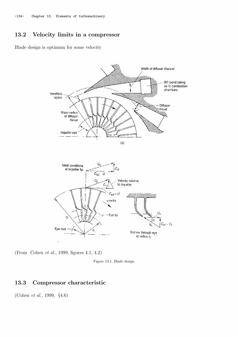
-134- Chapter 13. Elements of turbomachinery
13.2 Velocity limits in a compressor
Blade design is optimum for some velocity
(From Cohen et al., 1999, figures 4.1, 4.2)
Figure 13.1. Blade design
13.3 Compressor characteristic
(Cohen et al., 1999, §4.6)

13.3. Compressor characteristic -135-
Let us consider what might be expected to occur when a valve, placed in the delivery line of a
compressor running at constant speed, is slowly opened as illustrated in figure 13.2
p01
compressor vavle
p02
p01
p02
mout
mass flow rate
mout
0
A
B
1
C
C
constant speedcurve
E+
Figure 13.2. Compressor theoretical characteristic
• When the valve is shut and the mass flow is zero, the pressure ratio will reach some value
A, corresponding to the centrifugal pressure head produced by the action of the impeller on
the air trapped between the vanes.
• As the valve is opened and flow commences, the diffuser begins to contribute its quota of
pressure rise, and the pressure ratio increases from A to B
• At some point B, where the efficiency approaches its maximum value, the pressure ratio will
reach a maximum,
• and any further increase in mass flow will result in a fall of pressure ratio. For mass flows
greatly in excess of that corresponding to the design mass flow, the air angles will be widely
different from the vane angles, breakaway of the air will occur, and the efficiency will fall off
rapidly.
• In this hypothetical case the pressure ratio drops to unity at C, when the valve is fully
opened and all the power is absorbed in overcoming internal frictional resistance.
• There is an additional limitation to the operating range, between B and C. As the mass
flow increases and the pressure decreases, the density is reduced and the radial component of
velocity must increase. At constant rotational speed this must mean an increase in resultant
velocity and hence in angle of incidence at the diffuser vane leading edge. Sooner or later, at
some point (e.g. E), the position is reached where no further increase in mass flow can be
obtained and choking is said to have occurred. This point represents the maximum delivery
obtainable at the particular rotational speed for which the curve is drawn.

-136- Chapter 13. Elements of turbomachinery
13.3.1 Surge
In practice, most of the curve between A and B is instable and can not be obtained and surging
occurs.
Surging is associated with a sudden drop in delivery pressure, and with violent aerodynamic
pulsation which is transmitted throughout the whole machine.
Surge is a total low instability of the compressor flow system, which may be expected to occur
near the maximum pressure ratio of the characteristic but also depends on the flow dynamics of
the upstream and down stream ducts.
p01
p02
mout
0
1
B
surge
unsta
ble
stable
constant speed curve
A
A
B
C
Figure 13.3. Surge and rotating stall
13.3.2 Stall
Another important cause of instability and poor performance is stall. Stall occurs when the flow
separates from the leading edge of the rotor blades. It is a local instability of the flow, but may
propagate from one blade to another blade as in rotating stall. When there is any non-uniformity
in the flow or geometry of the channels between vanes or blades, breakdown in the flow in one
channel, say B in figure 13.3, causes the air to be deflected in such a way that channel C receives
fluid at a reduced angle of incidence and channel A at an increased incidence. Channel A then
stalls, resulting in a reduction of incidence to channel B enabling the flow in that channel to
recover. Thus the stall passes from channel to channel Rotating stall may lead to aerodynamically
induced vibrations resulting in fatigue failures in other parts of the gas turbine.
13.3.3 Compressor choice
The compressor is characterised by the curves giving its efficiency ηc as a function of the pressure
ratio p1
p2, the mass flow rate often given as m
√Tp
and the rotation rate often given as N√T:
In order to choose the compressor we have to superimpose the engine characteristics onto the

13.4. Real effects in exhaust turbine Systems -137-
from (6.46, 6.47 Heywood, 1988)) p. 261-262
Figure 13.4. Compressor characteristic diagrams
compressor characteristics:
From Stone (1999))figure 9.19 p. 392
Figure 13.5. Compressor choice
13.4 Real effects in exhaust turbine Systems
Actual operation may require some compromise between pulse and constant pressure designs,
depending on the number of cylinders and the engine duty.
• The ideal pulse system would have a turbine as close to the exhaust valve as possible,
implying one turbine per cylinder; not only is this impractical but there would be windage

-138- Chapter 13. Elements of turbomachinery
loss 75 % of the time for a 4 stroke engine.
• In practice several cylinders must be connected to the same turbine, so that the pulse energy
is partly dissipated in the connecting pipe system as well as at the exhaust valve restriction.
• Many diesel engines benefit from a scavenge through-flow of air during an extended valve
overlap period. This is only possible if pe ≪ pa during this time, and
a) each turbine entry is restricted to 2 or 3 cylinders unless pulse converters are used,
b) turbine housings then require divided inlet scrolls, leading to partial admission losses
due to windage and end of sector effects.
• Turbine efficiency oscillates during each engine cycle as the gas velocity changes, so that
a) average η < max η
b) apparent η > realη because pulse pressure > average pressure. For a well matched
system (e.g. 6 cylinder engine with 3 cylinders per turbine entry), the effect of b) is
usually greater than the combination of a) and the partial admission losses, particularly
at low engine load. Hence Pulse Factor > 1
• Pulse converters can be used to allow more cylinders to feed one turbine entry, by preventing
interference with scavenge.
• At high load and boost pressure1, some large engines effectively operate with a constant
pressure exhaust. If scavenge flow is not required, or for small engines at lower boost, a
constant pressure design is simpler and cheaper.
1The boost is the increase above atmospheric pressure of the induction pressure of a supercharged piston engine (Nayler,1985).

Revision questionnaire of Part III -139-
Revision questionnaire of Part III
1) What is the role of a turbocharger?
2) Explain what are constant pressure system and pulse system.
3) Give the definition and explain what is the pulse factor PF.
4) What are surge and stall in the context of turbines?
5) What are the swirl and radial component in a compressor?

-140- Revision questionnaire of Part III

part IV: Other reciprocating engines -141-
Part IV
Other reciprocating engines

-142- part IV: Other reciprocating engines

Chapter 14. Rotary Engine (Wankel Engine) -143-
Chapter 14: Rotary Engine (Wankel Engine)
See WebCT

-144- Chapter 14. Rotary Engine (Wankel Engine)

Chapter 15. HCCI Engine -145-
Chapter 15: HCCI Engine
See WebCT

-146- Chapter 15. HCCI Engine

Revision questionnaire of Part IV -147-
Revision questionnaire of Part IV
1) What is the main advantage of the Rotary or Wankel Engine
2) Describe the principle of HCCI engine

-148- Revision questionnaire of Part IV

Conclusion -149-
Conclusion

-150- Conclusion

List of Figures -151-
List of Figures
1.1 The four stroke operating cycle . . . . . . . . . . . . . . . . . . . . . . . . . . . . 19
1.2 Four stroke piston engine . . . . . . . . . . . . . . . . . . . . . . . . . . . . . . . . 19
1.3 Two stroke piston engine . . . . . . . . . . . . . . . . . . . . . . . . . . . . . . . . 20
1.4 Thermal efficiency . . . . . . . . . . . . . . . . . . . . . . . . . . . . . . . . . . . 20
2.1 Wet exhaust gas species concentration as a function of fuel/air φ equivalence ratio 25
2.2 Concentration in CO and CO2 in the products (dry) . . . . . . . . . . . . . . . . . 25
2.3 Energy of formation as a function of temperature . . . . . . . . . . . . . . . . . . 26
3.1 Example: heat exchange . . . . . . . . . . . . . . . . . . . . . . . . . . . . . . . . 32
4.1 Laminar premixed flame . . . . . . . . . . . . . . . . . . . . . . . . . . . . . . . . 37
4.2 Laminar flame speed as a function of φ at 1 bar . . . . . . . . . . . . . . . . . . . 38
4.3 Diffusion flame . . . . . . . . . . . . . . . . . . . . . . . . . . . . . . . . . . . . . 38
4.4 Tumble, Swirl and Squish . . . . . . . . . . . . . . . . . . . . . . . . . . . . . . . 40
4.5 Flame shape in a turbulent flow . . . . . . . . . . . . . . . . . . . . . . . . . . . . 41
4.6 Turbulent velocity definition . . . . . . . . . . . . . . . . . . . . . . . . . . . . . . 41
4.7 Turbulent flame compared to laminar flame . . . . . . . . . . . . . . . . . . . . . 42
4.8 Quenching near the walls . . . . . . . . . . . . . . . . . . . . . . . . . . . . . . . . 43
4.9 Diesel fuel spray combustion . . . . . . . . . . . . . . . . . . . . . . . . . . . . . . 43
4.10 Bunsen burner showing premixed and diffusion flames . . . . . . . . . . . . . . . . 44
5.1 Mass flux through the surface . . . . . . . . . . . . . . . . . . . . . . . . . . . . . 45
5.2 External normal convention . . . . . . . . . . . . . . . . . . . . . . . . . . . . . . 46
5.3 Mass flux through an elementary surface dσ . . . . . . . . . . . . . . . . . . . . . 46
5.4 The divergence theorem . . . . . . . . . . . . . . . . . . . . . . . . . . . . . . . . 48
5.5 Lagrangian derivative. The derivative is taken where the fluid particle is at time t. 50
5.6 Diffusion effect due to ~Vα > ~Vβ . . . . . . . . . . . . . . . . . . . . . . . . . . . . . 51
5.7 Diffusion effect. On the left, there is no diffusion: the mass fraction of red remains
constant on the fluid particle’s trajectory. On the right, red and white species diffuse
and their mass fractions change along the fluid particle’s trajectory. . . . . . . . . 51
5.8 Altering energy in a control volume . . . . . . . . . . . . . . . . . . . . . . . . . . 54
5.9 Energy conservation in a control volume . . . . . . . . . . . . . . . . . . . . . . . 55
5.10 Heat flux . . . . . . . . . . . . . . . . . . . . . . . . . . . . . . . . . . . . . . . . . 56

-152- List of Figures
5.11 Shear and pressure forces . . . . . . . . . . . . . . . . . . . . . . . . . . . . . . . . 57
5.12 Heat transfer due to mass transfer. . . . . . . . . . . . . . . . . . . . . . . . . . . 63
6.1 Swept volume for one cylinder . . . . . . . . . . . . . . . . . . . . . . . . . . . . . 71
6.2 Mean effective pressure pm . . . . . . . . . . . . . . . . . . . . . . . . . . . . . . . 73
7.1 Otto Cycle . . . . . . . . . . . . . . . . . . . . . . . . . . . . . . . . . . . . . . . . 77
7.2 Otto cycle efficiency . . . . . . . . . . . . . . . . . . . . . . . . . . . . . . . . . . 78
7.3 Indicator diagram for a spark ignition engine . . . . . . . . . . . . . . . . . . . . . 80
7.4 Effect of mixture equivalence ratio φ and flow velocity on minimum ignition energy
for propane-air mixtures et 0.7 atm . . . . . . . . . . . . . . . . . . . . . . . . . . 82
8.1 Carburettor . . . . . . . . . . . . . . . . . . . . . . . . . . . . . . . . . . . . . . . 86
8.2 Electronic fuel injection system . . . . . . . . . . . . . . . . . . . . . . . . . . . . 87
8.3 Spark engine performance . . . . . . . . . . . . . . . . . . . . . . . . . . . . . . . 88
8.4 Formation of dissociate product . . . . . . . . . . . . . . . . . . . . . . . . . . . . 89
8.5 3-way catalyst . . . . . . . . . . . . . . . . . . . . . . . . . . . . . . . . . . . . . . 90
8.6 Gas exchange process . . . . . . . . . . . . . . . . . . . . . . . . . . . . . . . . . . 91
8.7 Admission valve . . . . . . . . . . . . . . . . . . . . . . . . . . . . . . . . . . . . . 92
8.8 Electronic multipoint port fuel injection system L-Jelectronic system . . . . . . . 94
9.1 Diesel cycle . . . . . . . . . . . . . . . . . . . . . . . . . . . . . . . . . . . . . . . 97
9.2 Diesel sequence . . . . . . . . . . . . . . . . . . . . . . . . . . . . . . . . . . . . . 98
9.3 CI and SI φ regimes . . . . . . . . . . . . . . . . . . . . . . . . . . . . . . . . . . 101
9.4 Comparison of the part load efficiency 0f engines at 2000 rpm (Stone, R.) spark
ignition and Diesel . . . . . . . . . . . . . . . . . . . . . . . . . . . . . . . . . . . 102
10.1 Two stroke piston engine - scavenging . . . . . . . . . . . . . . . . . . . . . . . . . 103
10.2 Scavenge process in a two stroke engine . . . . . . . . . . . . . . . . . . . . . . . . 105
10.3 Perfect displacement scavenging . . . . . . . . . . . . . . . . . . . . . . . . . . . . 106
10.4 Complete mixing scavenging, as a function of λ . . . . . . . . . . . . . . . . . . . 107
10.5 Short circuit scavenging . . . . . . . . . . . . . . . . . . . . . . . . . . . . . . . . 107
10.6 Combined scavenge model . . . . . . . . . . . . . . . . . . . . . . . . . . . . . . . 108
11.1 Supercharging (left) and turbocharging (right) . . . . . . . . . . . . . . . . . . . . 115
11.2 Examples of superchargers, Roots blower, vane compressor, screw compressor . . . 116
11.3 Schematic of turbocharged engine system . . . . . . . . . . . . . . . . . . . . . . . 116
11.4 Example of turbochargers, left axial compressor right radial compressor . . . . . . 117
11.5 Enthalpy as a function of entropy diagram for a turbocharger . . . . . . . . . . . 118
List of Figures -153-
11.6 Typical arrangement of a constant pressure system . . . . . . . . . . . . . . . . . 119
11.7 Constant pressure system for several cylinders . . . . . . . . . . . . . . . . . . . . 120
11.8 Typical arrangement for pulse system . . . . . . . . . . . . . . . . . . . . . . . . . 120
11.9 Pulse generation . . . . . . . . . . . . . . . . . . . . . . . . . . . . . . . . . . . . 121
11.10Two-entry turbine inlet casing . . . . . . . . . . . . . . . . . . . . . . . . . . . . . 121
11.11Expansion energy available . . . . . . . . . . . . . . . . . . . . . . . . . . . . . . . 122
11.12Maximum p′em
p0as a function of p4
p0available from exhaust gases, with r ≫ 1 . . . . 123
11.13Expansion energy available . . . . . . . . . . . . . . . . . . . . . . . . . . . . . . . 123
11.14Energy available from a constant pressure exhaust manifold . . . . . . . . . . . . 124
11.15Maximum p′em as a function of pe for a constant pressure manifold, with p4 = 4 bar
and r ≫ 1 . . . . . . . . . . . . . . . . . . . . . . . . . . . . . . . . . . . . . . . . 125
12.1 Turbocharger . . . . . . . . . . . . . . . . . . . . . . . . . . . . . . . . . . . . . . 127
12.2 FIG. 10.11. Engine temperature rise factor K. . . . . . . . . . . . . . . . . . . . . 129
12.3 SFEE in the turbocharged engine . . . . . . . . . . . . . . . . . . . . . . . . . . . 130
13.1 Blade design . . . . . . . . . . . . . . . . . . . . . . . . . . . . . . . . . . . . . . . 134
13.2 Compressor theoretical characteristic . . . . . . . . . . . . . . . . . . . . . . . . . 135
13.3 Surge and rotating stall . . . . . . . . . . . . . . . . . . . . . . . . . . . . . . . . 136
13.4 Compressor characteristic diagrams . . . . . . . . . . . . . . . . . . . . . . . . . . 137
13.5 Compressor choice . . . . . . . . . . . . . . . . . . . . . . . . . . . . . . . . . . . 137

-154- List of Figures

Data sheets -155-
Data sheets
Data provided
Graph paper (if needed)
Steam table
Data book
Documents provided
Combustion temperature rise chart

-156- MEC403 Data sheets
Formulae
Scavenge ratio or delivery ratio λ
λ =ms
mi
Scavenge efficiency ηsc
ηsc =ma
ma + mg
Charging efficiency ηch
ηch =ma
mi
Trapping efficiency ηtr
ηtr =ma
ms=
ηch
λ
Where we used the following definition
vt : cylinder trapping volume
mi : ideal trapped air mass = ρsVt
ma : actual air mass in the cylinder
mg : mass of residual gas in the cylinder
ms : mass of air supplied to the cylinder
Perfect displacement : ηch = λ
Perfect mixing : dηch = dλ(1 − ηch)
Short circuit : dηch = 0
• Compressor polytropic efficiency
T02
T01=
(p02
p01
) γ−1
γηδc
• Turbine polytropic efficiency
T04
T03=
(p04
p03
) γ−1
γηδt

Data sheets -157-
• Choked nozzle
T5 =2
γ + 1T04 , V5 =
√γRT5
T5 static temperature of the jet, T04 total temperature after the turbine.
• Propulsive thrust
ηp =thrust power
total power
• Intake nozzle efficiency
ηi =T01′ − Ta
T01 − Ta
• propelling nozzle efficiency
ηj =T04 − T5
T04 − T5′

-158- MEC403 Data sheets
MEC403 Course Work -159-
Course Work
Introduction
You have to write a small report on a the 2-hour seminar given by Pr G. Kalghatgi.
Sustainable transport fuels for the future
6th December 2006 14:00 - 16:00
in SG LT14
Attendance is compulsory and an attendance list will be circulating.
The report should be between 3 to 5 pages including figures. The manuscript should be technically
well-written and organised. It should be your own work, not a compilation or scanning of different
book sections and web pages. Try to digest what has been done and present it in your own
words. Discuss information you gathered in a critical manner, as information coming from different
sources can be inconsistent or contradictory. Not being able to understand what has been done,
but attempting to know why can indicate maturity rather than lack of intelligence or knowledge.
The main purpose of this exercise is to train you to analyse and synthesise information and show
your ability to carry out literature survey.
Format
TITLE
Please have information as follows on the first page
• Module title and reference
• Lecturer’s name (in case your report get misplaced)
• Your name and email
• Your course (e.g. MEng., Erasmus, ...)
There is no a priori good or bad way to write a report. As long as you have valid reasons for your
report presentation. The model that follows is indicative and only here to help you.

-160- MEC403 Course Work
ABSTRACT or summary
INTRODUCTION & BACKGROUND
Briefly describe what you are presenting and why it is important.
STATE OF THE ART
The different designs or technologies. Their historic development. The current trends, the future
trends.
State what you think are their shortcomings
State concisely and specifically the researches that address one or more of the problems you have
cited.
REFERENCES
List carefully your references. You can find the books cited in this course at Saint Georges’ library.
But you can carry out your own literature survey and find much more.
Deadline and submission
You can submit your report in hand or send it by email if you choose to type it. Deadline is fixed
to week 12, Friday 15th December 2006 by 17.00. Late submission will be penalised. There is no
way I can know if a report is missing but I will acknowledge all reception by email (in January).
It is your responsibility to ensure that I got the report.

Solutions to exercises -161-
Solutions to exercises

-162- Solutions to exercises

Solutions of Chapter 2 -163-
Exercises of Chapter 2
Exercise §2.1.1
a)
C8H18 + na ( O2 + 7921
N2) → nCO2CO2 + nH2O H2O + na
7921
N2
Balance ofC : 8 = nCO2
nCO2= 8
H : 18 = 2nH2O nH2O = 9
O : 2na = 2nCO2+ nH2O na = 25
2
Hence stoichiometric equilibrium is:
C8H18 + 252
( O2 + 7921
N2) → 8 CO2 + 9 H2O + 197542
N2
Stoichiometric fuel/air (mass) ratio:
fst =mass of fuel
mass of air=
12 × 8 + 12252
(2 × 16 + 79
21× 2 × 14
) =1145150
3
=342
5150= 0.0664
b)
Use Rogers & Mayhew (1998) page 21
∆h = −5116180 kJ.kmol−1
Hence
∆h = fst1
mf∆h = 0.0664 × 1
8 × 12 + 18︸ ︷︷ ︸mol.g−1
× 5116180︸ ︷︷ ︸J.mol−1
J.g−1 of air
∆h = −2979.95 kJ.kg−1 of air
(note the convention sign − indicates energy is released to the exterior)
c)
If all liquid
∆h = −5116180 + hfg(C8H18) − 9 × hfg(H2O)
∆h = −5116180 + 41500 − 9 × 43990 = −5470590 kJ.kmol−1
∆h = 0.0664 × 1
8 × 12 + 18× (−5470590) = −3186 kJ.kg−1

-164- Solutions of Chapter 2
e)
∆H − ∆U = ∆(pV ) = (nP − nR)RT
which for 1 kmol of octane is 3.5 × 8.3145 × 298 = 8672 kJ.kmol−1 i.e.
∆u = ∆h − ∆(pV ) = −2980 − 5 = −2985 kJ per kg of air

Solutions of Chapter 3 -165-
Exercises of Chapter 3
Exercise §3.5.3
a)
a (H2 +1
2O2)
︸ ︷︷ ︸stoichiometric
→ nh2oH2O + nPh2
H2 + nPo2
O2
5 % of the original H2 remains uncombined: nPh2
= 0.05a
Balance ofH : a = nh2
+ nh2o nh2o = a − 0.05a = 0.95a
O : a = nh2o + 2no2no2
= 12(1 − 0.95)a = 0.025a
We have equilibrium in the products as follows
H2 +1
2O2 H2O
K−(T ) =pH2O
pH2(pO2
)1
2
(p−) 1
2
With
pH2=
nh2
nP pP = 0.051.025
pP = 0.0488 × pP
pO2=
no2
nP pP = 0.0251.025
pP = 0.0244 × pP
pH2O =nh2o
nP pP = 0.951.025
pP = 0.927 × pP
where nP = nh2o + nPh2
+ nPo2
= (0.05 + 0.95 + 0.025)a = 1.025a. Hence
K−(T ) =0.927
0.0488 × 0.02441
2
×(
1
10
) 1
2
= 38.46
b)
Looking in table (Rogers & Mayhew, 1998) page 21 for T such that
K−(T ) = 38.5 i.e. ln K−(T ) = 3.65
we find T = 2844 K
c)
Initially TR = 25C = 298 K. If we assume ideal gas
pRV = nRRTR

-166- Solutions of Chapter 3
and
pP V = nP RTP
both mixtures, reactants and products, are in the same volume V , hence
pR
pP
=nR
nP
TR
TP
that is
pR =nR
nP
TR
TPpP =
(1 + 12)a
1.025a× 298
2844× 10 = 1.53 bar
d)
For a close volume first law of thermodynamics is
∆U = Q − W
with here W = 0 the heat gained by the bomb per kmol of H2 is
q = ∆u = ∆h − ∆(pV ) = ∆h − ∆(nRT ) = ∆h − R(nPTP − nRTR)
Only 95 % of the initial number of moles of H2 has reacted and the products are at the temperature
TP = 2844 K. Hence
∆h = 0.95 ∆h− + nh2o∆h(H2O)298→2844 + nh2∆h(H2)298→2844 + no2
∆h(O2)298→2844
∆h = 0.95 × (−241 830) + 0.95 × 117 725 + 0.05 × 82 992 + 0.025 × 91 893 = −111 452 kJ.kmol−1
so that
q = −111 452 − 8.3145 × (1.025 × 2844 − 1.5 × 298) = 131 973 kJ per kmol of H2
and dividing by the molar mass of H2 that is 2 kg.kmol−1
q = 65 986 kJ.kg−1
Exercise §3.5.4
φ C8H18 +25
2
(O2 +
79
21N2
)→ ncoCO + nco2
CO2 + nh2oH2O + nh2H2 + nn2
N2
Balance of
N : 252× 79
21= nn2
⇒ nn2= 1975
42
H : 18φ = 2nh2o + 2nh2⇒ nh2o = 9φ − nh2
C : 8φ = nco + nco2⇒ nco = 25(φ − 1) − nh2
O : 25 = nco + 2nco2+ nh2o ⇒ nco2
= 25 − 17φ + nh2

Solutions of Chapter 3 -167-
We need an additional relation to close the problem. We have the equilibrium at 1200 K in the
products
CO2 + H2 CO + H2O
Which yields:
K−(1200 K) =pH2OpCO
pH2pCO2
= e0.311 = 1.3648
that is
K− =
nh2o
nP × nco
nP
nh2
nP × nco2
nP
=nh2o × nco
nh2× nco2
Hence we have to solve for nh2
(25(φ − 1) − nh2)(9φ − nh2
) − K−(1200 K)(−17φ + 25 + nh2)nh2
= 0
or with φ = 1.1
(2.5 − nh2)(9.9 − nh2
) − 1.3648(6.3 + nh2)nh2
= 0
We find nh2= 1.156 and
nco = 1.344
nco2= 7.456
nh2o = 8.744
nn2= 47.02
np = nh2+ nco + nco2
+ nh2o + nn2
= 1.156 + 1.344 + 7.456 + 8.744 + 47.02 = 65.72
Hence
xh2=
nh2
nP = 1.76%
xco = nco
nP = 2.04%
xco2=
nco2
nP = 11.3%
xh2o =nh2o
nP = 13.3%
xn2=
nn2
nP = 71.6%
Exercise §3.5.5
? + a(O2 +
79
21N2
)→ a
4O2 + nnoNO + nn2
N2 + ?
Balance of
N : a7921
= nn2+ nno
In the products we have equilibrium for the reaction
1
2N2 +
1
2O2 NO

-168- Solutions of Chapter 3
Hence
K−(2200 K) =pNO
(pN2)
1
2 (pO2)
1
2
that is
K−(2200 K) =nno
(nn2)
1
2 (no2)
1
2
or
K−(2200 K) =nno
(nn2)
1
2 (no2)
1
2
that is when substituting for no2and nn2
(K−(2200 K)
)2 a
4
(79
21a − nno
)= (nno)
2 (15.1)
The proportion of nitrogen N2 converted into NO is nno
a 79
21
dividing both sides of equation (15.1)
yields:(K−(2200 K)
)2 1
4
(79
21− nno
a
)=(
nno
a
)2
we have to solve
0.03282(3.76 − nno
a) =
(nno
a
)2
we find nno
a= 0.0317 so that 0.0317/79
21= 8.42 % of initial N2 has been converted into NO (or
4.21 % of initial N).
Exercise §3.5.6
a)
φ CO + 12
( O2 + 7921
N2) → nco2CO2 + nco CO + nn2
N2 + no2O2
Balance ofC : φ = nco2
+ nco (1)
O : φ + 1 = 2nco2+ nco + 2no2
(2)
N : nn2= 79
42(3)
With φ = 1.1 (10 % rich mixture) we are left with 3 unknowns:
nco2, nco and no2
and two equations (1) and (2)
the products resulting from the combustion are in equilibrium at 3000 K and pP = 40 bar, hence:
CO2 CO + 12
O2
K−(3000 K) =pCO2
(p−)1
2
pCO (pO2)
1
2
(15.2)

Solutions of Chapter 3 -169-
is the closing equation to solve for the 3 unknown coefficients. Partial pressure are related to the
total pressure pP :
pCO2=
nco2
nP pP
pO2=
no2
nP pP
pCO = nco
nP pP
where nP is the total number of moles in the products nP = nco2+ nP
o2+ nP
co + nPn2
equation (15.2)
becomes
K−(3000 K) =
nCO2
nP pP (p−)1
2
nPCO
nP pP
(nO2
nP
) 1
2 pP1
2
that is
K− =nCO2
nPCO
×(
nP
nO2
) 1
2
×(
p−
pP
) 1
2
or
K−2(nP
co
)2nO2
= (nco2)2 nP
(p−
pP
)(15.3)
We have three unknowns and three equations let us choose to solve for nco2and substitute the
other unknowns. We have
from (1) nco = φ − nco2
from (1) and (2) no2=
1−nco2
2
then nP = φ + nn2+
1−nco2
2
Substituting in equation (15.3):
(K−)2 (nco2)2(
1 − nco2
2
)= (nco2
)2(φ + nn2
+1 − nco2
2
)(p−
pP
)
Hence we have to solve:
(3.034)2(1 − nco2)(1.1 − nco2
)2 − (nco2)2(6.96 − nco2
)1
40= 0
Try some values until convergence → nco2= 0.835 mol then
nco = 0.265
no2= 0.0825
nP = 3.06
For 1.1 mol of CO supplied 0.265 are present in the products that is 24 % and the molar gas
composition is:
xco2= 0.835
3.06= 27.3%
xco = 0.2653.06
= 8.7%
xo2= 0.0825
3.06= 2.7%
xn2= 1.88
3.06= 61.5%

-170- Solutions of Chapter 3
b)
φ CO + 12
( O2 + 7921
N2) → nco2CO2 + nco CO + nn2
N2 + no2O2 + nno NO
Balance ofC : φ = nco2
+ nco (1)
O : φ + 1 = 2nco2+ nco + 2no2
+ nno (2)
N : 2nn2+ nno = 79
21(3)
With φ = 1.1 (10 % rich mixture) we are left with 5 unknowns:
nco2, nco, no2
, nn2and nno and three equations (1), (2) and (3)
• there still is equilibrium for CO:
CO2 + 12
O2 CO
and equation (15.3) still holds but now nP = nco2+ nP
co + nPo2
+ nPn2
+ nno
• There is also equilibrium for NO12
N2 + 12
O2 NO
and the additional equation needed to close the problem is
K−n2
(3000 K) =pno
(po2)
1
2 (pn2)
1
2
=nno
(no2)
1
2 (nn2)
1
2
That is(K−
n2
)2no2
nn2= (nno)
2 (15.4)
We can choose to keep nco2and nno and substitute other unknowns in equations (15.4) and (15.3)
we end up with:(K−
n2
)2(1 − nco2
− nno)(
79
21− nno
)= 4 (nno)
2 (15.5)
and(K−
co2
)2(1 − nco2
− nno)(φ − nco2)2 = (nco)
22φ +
79
21+ (1 − nco2
)
1
40(15.6)
We can use previous value for nco2(0.835) in (15.5) and find nno value for which (15.5) is verified:
nno = 0.0414
we then use this value in (15.6) to get update the value for nco2, we get:
nco2= 0.818
then carry on until convergence of nno and nco2, i.e. use nco2
= 0.818 in (15.5) it yields
nno = 0.0438

Solutions of Chapter 3 -171-
and then use nno = 0.0438 in (15.6) it yields
nco2= 0.817
Considering these two latter values as converged we get:
nPco = φ − nco2
= 1.1 − 0.817 = 0.283
nPn2
= 12
(7921
− nno
)= 1.859
nPo2
= 12(1 − nco2
− nno) = 0.0696
nP = 0.817 + 0.283 + 1.859 + 0.00696 + 0.0438 = 3.0724
For 1.1 mol of CO in the reactants there are 0.283 mol in the products that is 25.7% and the
molar gas composition is
xco2= 0.817
3.0724= 26.6%
xco = 0.2833.07
= 9.2%
xo2= 0.0696
3.07= 2.26%
xn2= 1.859
3.07= 60.5%
xno = 0.04383.07
= 1.4%

-172- Solutions of Chapter 3

Solutions of Chapter 6 -173-
Exercises of Chapter 6
Exercise §6.3
a)
The brake mean effective pressure is defined as
pbm =Wb
Vs
with
Wb = ηthb × mfuel × LCV
where
mfuel =mair
α= ηvol × ρair
1
αVs
Hence
pbm =Wb
Vs= ηthb × ηvol × ρair
1
αLCV
that is
pbm = 0.35 × 0.80 × 1.201 × 1
15× 44000 = 986.42 kPa = 9.9 bar
The brake specific fuel consumption is:
bsfc =mfuel
Wb=
1
ηthb× 1
LCV=
1
0.35× 1
44 × 106= 6.49 10−8 kg.J−1 = 0.234 kg.(kWh)−1
b)
The work per cycle, that is in a 4-stroke engine per four strokes is
Wcycle = pbmVs
the work per revolution that is per two strokes is (equation 6.2)
Wrev = 2πτ
Hence
τ =Wrev
2π=
Wcycle
2
2π=
Wcycle
4π=
9.9 × 105 × 2 × 10−3
4π= 157 N.m
c)
The brake power is
W = τ.Ω = τ.2πN
60= 157 × 2 × π
3000
60= 49.3 kW

-174- Solutions of Chapter 6
d)
In previous condition the air was occupying a volume Va = Vs now as it is mixed with natural gas
it occupies a volume V ′a and the gas a volume V ′
g = V ′
a
10and the mixture of the two gases fills in
previous volume Va:
Vs = Va = V ′a + V ′
g = 1.1V ′a
hence V ′a = 1
1.1Va and the new volumetric efficiency is
η′vol =
m′a
ρaVs=
ρaV′a
ρaVs=
ρaVa1
1.1
ρaVs=
1
1.1ηvol =
0.8
1.1≃ 0.73

Solutions of Chapter 7 -175-
Exercises of Chapter 7
Exercise §7.1.1
a-i)
From equation (7.2)
ηc = 1 − 1
rvγ−1
= 1 − 1
101.4−1 = 0.602
a-ii)
We haveT2
T1=(
V1
V2
)γ−1
= rvγ−1 =
(V4
V3
)γ−1
=T3
T4
and
p1V1 = nRRT1
p2V2 = nRRT2
p3V2 = nP RT3
p4V1 = nP RT4
Here we are using air throughout the cycle: nP = nR and p1V1
p3V2= T1
T3that yields
T3 = T1p3
p1× V2
V1= T1
p3
p1× 1
rv= 300 × 100
1× 1
10= 3000 K
a-iii)
T2 = T1rvγ−1 = 300 × 100.4 = 753.6 K
the specific heat is then
q2−3 = cv(T3 − T2) = 0.7178 × (3000 − 753) = 1612 kJ.kg−1
a-iv)
T4 =T3
rvγ−1
=3000
100.4= 1194 K
andp3
p4
× v2
v1
=T3
T4
yields
p4 =T4
T3× v2
v1× p3 =
1194
3000× 1
10× 100 = 3.98 bar

-176- Solutions of Chapter 7
a-v)
pmVs = W = ηcQ = ηcm1q = ηcqVsρ1
Hence
pm = ηcqρ1
for ρ1 use the equation of states for ideal gas
v1 = RT1
p1= 8.3145 × 300
105= 0.0249 m3.mol
−1
and
ρ1 =1
v1=
m
v1=
29 × 10−3
0.0249= 1.16 kg.m−3
or use table Rogers & Mayhew (1998) page 16 (ρ1 = 1.177) then
pm = 0.602 × 1612 × 103 × 1.16 Pa = 11.28 bar
b)
From previous section T2 = 754 K and T3 = 3000 K, T1−2 = 754+30002
= 1877 K. From tables page
16 at 1 bar, γ = 1.301 and cv = 0.9534 kJ.kg−1.K−1
i)
ηc = 1 − 1
rvγ−1
= 1 − 1
100.3= 49.9%
iii)
Q2−3 = cv(T3 − T2) = 0.9534 × 10⁻³(300 − 754) = 2142 kJ
c)
From tables page 21
∆h− = −5 116 180 kJ.kmol−1
at 298 K, octane reaction is
C8H18 +25
2
(O2 +
79
21N2
)→ 8CO2 + 9H2O +
79
21× 25
2N2
Hence for each kmol of fuel there is 12.5 kmol of O2 that is 12.5 × 10.21
= 59.52 kmol of air
59.52 × mair = 59.52 × 29 = 1726.2 kg of air per kmol of fuel
the energy delivered per kmol of fuel is
∆h =∆h−
1726.2= 2964 kJ.kg−1 of air

Solutions of Chapter 8 -177-
Exercises of Chapter 8
Exercise §8.8.1
Vpmax =1 stroke
time to do 1 stroke= S︸︷︷︸
1 stroke per
half revolution
N × 2︸ ︷︷ ︸number of
half revolution
per 2 strokes
with S the strokes and N in rev.s−1.
Furthermore for Vmean the piston mean velocity:
Vpmax = 1.62 × Vmean = 1.62 × 2 × NS = 3.24 NS
Continuity (mass conservation) requires
ApVp = Aef︸︷︷︸effective area
Vv = CDAgVv
at any time. In particular at the discharge Vp and Vv are maximum:
ApVpmax = Aef (Vp)disch
From Bernouilli on the valve we have
p1 + 0 = p2 +1
2ρV2
2
or
∆p =1
2ρV2
2
with ρ(1 bar, 300 K) = 1.177. Hence on the valve
(∆p)disch =1
2ρ(V2
v
)
disch
so that
Vpmax = 3.24 × NS = CDAg
Ap
(V2
v
)
disch= CD
Ag
Ap
√2∆p
ρ
Hence
N =1
3.3× CD
S
Ag
Apsqrt
2∆p
ρ
in rev.s−1
N = 18.52 × CD
S
Ag
Apsqrt
2∆p
ρ
in rev.min−1

-178- Solutions of Chapter 8
• N ′ = 4438 rev.min−1 for Ag
Ap= 0.2 and
• N ′ = 5770 rev.min−1 for Ag
Ap= 0.26

Solutions of Chapter 10 -179-
Exercises of Chapter 10
Exercise §10.3.6
For 0 < λ < 0.3, the scavenging process is perfect displacement:
ηch = λ
and this fixes the boundary condition ηch = 0.3 for λ = 0.3
90 % of further fresh charge is mixing scavenge dηch = dλ(1 − ηch) and the 10% remaining is
short-circuit dηch = 0 so the total charge efficiency increment is
dηch = 0.9dλ(1 − ηch)
that is
dλ =dηch
0.9(1 − ηch)
which can be integrated from λI = 0.3 to λ
λ − λI =∫ ηch
ηchI
dηch
0.9(1 − ηch)= − 1
0.9ln(
1 − ηch
1 − λI
)
or
1 − ηch = e−0.9(λ−λI )(λ − λI)
that is with λI = 0.3
ηch = 1 − 0.7 × e0.9×0.3 × e−0.9λ = 1 − 0.917 × e−0.9λ
For a unit scavenge ratio λ = 1
ηch = 1 − 0.7 × e0.9×0.3 × e−0.9×1 = 0.627
For mixing scavenge throughout
ηch = 1 − e−λ = 1 − e−1 = 0.632
Exercise §10.4.1
a)
The work lost in the port is
W =∫
V dp = Vt∆p ≃ Vs∆p

-180- Solutions of Chapter 10
the actual work lost by the compressor of efficiency ηc is
Wc =W
ηc=≃ Vs
∆p
ηc
and terms of mean effective pressure
plost =Wc
Vs
=∆p
ηc
=0.25
0.85= 0.29 bar
b)
According to exercise §10.3.6
ηch = 1 − 0.917 × e−0.9λ
or
λ = − 1
0.9ln(
1 − ηch
0.917
)
that is for ηch = 0.8, λ = 1.69. If we can neglect density change and ∆p ∼ λ2 we can use relation
(10.5):
plost =Wc
Vs
= cλ3
where c can be deduced from a)
plost =0.29
13× 1.693 = 1.4 bar
Neglecting density change seems a strong assumption with ∆p = 1.4

Solutions of Chapter 11 -181-
Exercises of Chapter 11
Exercise §??
a)
Use equation (11.7) with r ≪ 1
p′em =W ′
max
Vs≃ p0
1 +
1
γ − 1
(p4
p0
)− γ
γ − 1
(p4
p0
) 1
γ

-182- Solutions of Chapter 11

Solutions of Chapter 12 -183-
Exercises of Chapter 12
Exercise §12.6
a)
pem = aρa
pe = bpa
Te = cTa
At 30C, 1 bar ρa = 1.177 kg.m−3 (table Rogers & Mayhew (1998) page 16), hence
a = pem
ρa= 10
1.177= 8.5 bar.m3.kg−1
b = pe
pa= 3.5
1= 3.5
c = Te
Ta= 800+273
30+273= 3.54
Now the inlet pressure of the cylinder is pa = 1.8 bar, use relations (11.3) and (11.6) to find the
temperature after the compressor that is the temperature in the cylinder.
ηc =Tas − T0
Ta − T0
with Tas
T0=(
pa
p0
) γa−1
γa , hence
ηc =
T0
[(pa
p0
) γa−1
γa − 1
]
Ta − T0
and
Ta = T0
1 +1
ηc
(
pa
p0
)γa−1
γa
− 1
= 303 ×
1 +1
0.7
(
1.8
1
) 1.4−1
1.4
− 1
= 382.2 K
from ideal gas equation before and after the compressor we get p0
pa
ρa
ρ0= T0
Tathat is
ρa = ρ0T0
Ta
pa
p0= 1.177 × 303
382.2× 1.8
1= 1.68 kg.m−3
and
piem = 8.5 × ρa = 8.5 × 1.68 = 14.28 bar
pe = 3.5 × pa = 3.5 × 1.8 = 6.3 bar
at the turbine inlet the temperature is
Te = 3.54 × Ta = 3.54 × 382.2 = 1353 K = 1080C

-184- Solutions of Chapter 12
b)
Power balance requires Wt = Wc that is
cpa(Ta − T0) = cpe(Teo − Te)
or
γa
γa − 1T0
1
ηc
(
pa
p0
) γa−1
γa
− 1
=
γg
γg − 1Teηt
(
p0
pe′
)γg−1
γg
− 1
were pe′ is the constant pressure in the exhaust manifold or at the turbine inlet, then
pe′ = p0
1 − γa
γa − 1
γg
γg − 1
T0
Te
1
ηcηt
(
pa
p0
) γa−1
γa
− 1
γg1−γg
that is
pe′ = 1 × 105 ×
1 − 7
2
1
4
303
1353
1
0.7 × 0.7
[(1.8
1
)−4
− 1
]−4
= 1.35 × 10⁵ Pa
Exercise §12.7
a)
∆T = Te − Ta =1200
1 + 20= 571 K
For a perfect gas the compressor efficiency is
ηc =Tsa − T0
Ta − T0
with Tsa the isentropic temperature. Hence
Ta = T0 +1
η(Tsa − T0) = T0
1 +
1
η
(
pa
p0
) γ−1
γ
− 1
= 293×
1 +
1
0.75
(
1.6
1
) 2
7
− 1
= 349 K

Solutions of Chapter 12 -185-
Hence turbine inlet temperature is Te = Ta + ∆T = 349 + 571 = 920 K..
The actual work in the compressor is
Wc =ma
ηccpaT0
(
pa
p0
) γ−1
γ
− 1
and the turbine efficiency is for a perfect gas
ηt = PF × ηts =Te0 − Te
Teos − Te
=Wt
Wts
and the actual work from the turbine is
Wt = ηtmecpeTe
1 −
(p0
pe
) γe−1
γe
with me = ma + mf = (1 + f)ma. The turbine provides the work for the compressor, Wt = Wc:
maηt(1 + f)γeR
γe − 1Te
1 −(
p0
pe
)γe−1
γe
= maγaR
γa − 1(Ta − T0)
Hence
Te
1 −
(p0
pe
)γe−1
γe
=
γa(γe − 1)
γe(γa − 1)(Ta − T0)
1
ηt(1 + f)
thereforep0
pe=
[1 − γa(γe − 1)
γe(γa − 1)
(Ta
Te− T0
Te
)1
ηt(1 + f)
] γeγe−1
or
pe = p0
[1 − γa(γe − 1)
γe(γa − 1)
(Ta
Te− T0
Te
)1
ηt(1 + f)
] −γeγe−1
(15.7)
That is
pe = 1 × 105 ×[1 − 7
2× 1
4×(
349
920− 293
920
)× 1
0.65 × 1.2 × (1 + 120
)
]−4
= 1.31 × 10⁵ Pa
b)
We still have
Ta = T0 +1
ηc(Tsa − T0) = T0
1 +
1
ηc
(
pa
p0
) γa−1
γa
− 1
but now p0 = 0.8, ηc = 0.7, hence,
Ta = 293 ×1 +
1
0.7
(
1.6
0.8
) 2
7
− 1
= 384.7 K

-186- Solutions of Chapter 12
The air mass flow is proportional to compressed air density:
at p0 = 1 bar α = ma
mf
at p0 = 0.8 bar α′ = m′
a
mf
henceα′
α=
m′a
ma=
ρ′a
ρa=
p′aT ′
a
× Ta
pa=
Ta
T ′a
=349
384.7= 0.907
(since pa = p′a = 1 bar) then
T ′e = T ′
a + ∆T ′ = T ′a +
1200
1 + α′= T ′
a +1200
1 + 0.907 × α= 384.7 +
1200
1 + 0.907 × 20= 1012 K
and relation (15.7) is still valid:
pe = 0.8 × 105 ×[1 − 7
2× 1
4×(
384.7
1012− 293
1012
)× 1
0.6 × 1 × (1 + 118.14
)
]−4
= 1.366 × 10⁵ Pa

References -187-
References
Beck, S. B. M. 2000 MEC 108: Heat, Work and Energy . First year notes, Mechanical
Engineering, The University of Sheffield.
Boas, M. L. 2005 Mathematical Methods in the Physical Sciences , 3rd edn. Wiley.
Cengel, Y. A. & Boles, M. A. 1998 Thermodynamics An Engineering Approach, 3rd
edn. Mc Graw Hill.
Cohen, H., Rogers, G. F. C. & Saravanamuttoo, H. I. H. 1999 Gas Turbine Theory ,
4th edn.
Fergusson, C. R. 1986 Internal Combustion Engines Applied Thermosciences. John Wiley
& Sons.
Flynn, P. F., Durrett, R. P., Hunter, G. L., zur Loye, A. O. & Akinyemi,
O. C. 1999 Diesel Combustion: An integrated View Combining Laser Diagnostics, Chemical
Kinetics, and Empirical Validation. SAE paper Series 1999-01-0509 .
Heywood, J. B. 1988 Internal combustion engine fundamentals. MacGraw-Hill.
Heywood, J. B. & Sher, E. 1999 The Two-Stroke Cycle Engine. Taylor & Francis.
Lumley, J. 1999 Engines an introduction. Cambridge University Press.
Nayler, G. H. F. 1985 Dictionary of Mechanical Engineering , 4th edn.
Nicolleau, F. 1994 Processus fractals et reaction chimique en milieux turbulents. PhD
thesis, Ecole Centrale de Lyon.
Nicolleau, F. 2001 MEC310 Energy properties and optimisation. Department of Mechan-
ical Engineering the University of Sheffield.
Nicolleau, F. & Mathieu, J. 1994 Eddy Break Up Model and Fractal Theory - Compar-
isons with Experiments. Int. J. Heat Mass Transfer. 37 (18), 2925–2933.
Peters, N. 2000 Turbulent Combustion. Cambridge University Press.
Rogers, G. F. C. & Mayhew, Y. R. 1998 Thermodynamic and transport properties of
fluids , 5th edn. Blackwell.

-188- References
Smyth, R. 1999 Thermodynamics and Heat Transfer . Mechanical Engineering, University
of Sheffield: Second year notes, Mechnical Engineering, The Universiyt of Sheffield.
Stone, R. 1999 INtroduction to Internal Combustion Engines, 3rd edn.

References -189-