Francesco Bertoluzzo and

Marco Corazza

Reinforcement Learning for automatic financial trading:

Introduction and some applications

ISSN: 1827/3580 No. 33/WP/2012

W o r k i n g P a p e r s

D e p a r t me n t o f E c o n o m i c s

C a ’ Fo s c a r i U n i v e r s i t y o f V e n i c e

N o . 3 3 / W P / 2 0 1 2

ISSN 1827-3580

Reinforcement Learning

for automatic financial trading:

Introduction and some applications

Francesco Bertoluzzo (fbertoluzzo@unive.it)

Department of Economics

Ca' Foscari University of Venice

Marco Corazza (corazza@unive.it)

Department of Economics

Ca' Foscari University of Venice

and

Advanced School of Economics of Venice

First Draft: December 3, 2012

Abstract

The construction of automatic Financial Trading Systems (FTSs) is a subject of research of high interest for both academic environment and financial one due to the potential promises by self-learning methodologies and by the increasing power of actual computers. In this paper we consider Reinforcement Learning (RL) type algorithms, that is algorithms that optimize their behavior in relation to the responses they get from the environment in which they operate, without the need for a supervisor. In particular, first we introduce the essential aspects of RL which are of interest for our purposes, then we present some original automatic FTSs based on differently configured RL algorithms and apply such FTSs to artificial and real time series of daily financial asset prices.

Keywords

Financial Trading System; Reinforcement Learning; Stochastic control; Q-learning algorithm; Kernel-based Reinforcement Learning.

JEL Codes

C61; C63; D83; G11.

Address for correspondence:

Marco Corazza

Department of Economics Ca’ Foscari University of Venice

Cannaregio 873, Fondamenta S.Giobbe

30121 Venezia – Italy Phone: (++39) 041 2346921

Fax: (++39) 041 2349176

E-mail: corazza@unive.it This Working Paper is published under the auspices of the Department of Economics of the Ca’ Foscari University of Venice. Opinions expressed herein are those of the authors and not those of the Department. The Working Paper series is designed to divulge preliminary or incomplete work, circulated to favour discussion and comments. Citation of this paper should consider its provisional character.

1 Introduction

Many resources have been recently spent among professionals as well as in the academic worldin searching for automaticFinancial Trading Systems (FTSs) that can substitute for experience,capacity, and intuition human operators in the choice of investments in financial markets.

In the specialized literature several different approaches have been considered to address sucha problem: Statistical and econometric models using, amongothers, macroeconomic indicators;Simpler and flexible models based on the Technical Analysis indicators; Models based on machinelearning that make extensive use of computing capacity.

In this paper we consider a class of self-adaptive algorithms for dealing with the above problemin order to obtain profitable and fully automatic FTSs. In particular, the methodology we consider isknown asReinforcement Learning(RL) [1] also known asNeuro-Dynamic Programming[2]. In ourapproach, investment decision making is viewed as a stochastic control problem and the investmentstrategies are discovered directly interacting with the market. So, the need to build forecastingmodels for future prices or returns is eliminated.

In literature there are many contributions in this researchfield. Among the ones we recall [6],[7], and [5]. In general, they show that such strategies perform better than the ones based on super-vised learning methodologies when market frictions are considered. In [6] a simplified version ofRL algorithm, called Direct Learning, is used in order to seta FTS that, taking into account trans-action costs, maximizes an appropriate investor’s utilityfunction based on a differential version ofthe well-known Sharpe ratio. Then, they show by controlled experiments that the proposed FTSperforms better than standard FTSs. Finally, the authors use their FTS to make profitable tradeswith respect to assets of the U.S. financial markets. In [7], the authors mainly compare FTSs devel-oped by using RL methodologies with FTSs developed by using stochastic dynamic programmingmethodologies. In general they show by extensive experiments that the former approach is betterthan the latter one. In [5] the author considers an FTS similar to the one developed in [6] and appliesit to the financial high-frequency data, obtaining profitable performances.

With respect to the prominent literature, in this paper we will do the following:

• We will develop and we will apply FTSs based on two different RL approaches, namely theTemporal Differenceone (see subsection 2.3) and theKernel-based Reinforcement Learning(see subsection 2.4);

• Beyond to consider the usual buy and sell signals, we will take into account also a third signal:The stay-out-from-the-market one;

• Instead of using the differential Sharpe ratio as performance indicator, we will utilize theclassical Sharpe ratio computed on the lastL ∈ N trading days.

The remainder of the paper is organized as follows: In section 2 we will introduce the essentialaspects of RL which are of interest for our purposes; In section 3 we will present our RL-basedFTSs and we will provide the results of their applications toartificial and real time series; In section4 we will give some concluding remarks.

2 Reinforcement Learning

Learning by interacting directly with the environment without the need of a supervisor is likely themore immediate idea about the nature of learning. The consequences of the actions of the learner(agent) lead the agent himself to choose what are the actionsthat allow to obtain the desired resultsand what are the ones to avoid. RL formalizes this kind of learning by maximizing a numericalreward ([1]). The agent has to discover which actions yield the most reward by trying them. RLis different from Supervised Learning (SL) in which the agent learns from examples provided byan external supervisor. SL is an important kind of learning,but in interactive problems it is oftenimpractical to obtain examples of desired behavior that arerepresentative of the situation in whichthe agent has to act. In uncharted and unknown environments (like, for instance, financial markets)the agent must to be able to learn only from its own past experience.

To formalize these first ideas, let us consider a system observed at discrete time steps in whichthe state at time stept, st ∈ S , summarizes all information concerning the system available to theagent. In the RL framework it is assumed that the system satisfies the Markov property, that isthat the probability of transition from the actual statest to the next onest+1 depends only on thecurrent statest . On the basis ofst , the agent selects an actionat ∈ A (st), whereA (st) is the setof all possible actions the agent can take given the statest . At time stept +1 the agent receives areward,r(st ,at ,st+1) ∈ R, as consequence of his actionsat and of the new statest+1 in which hefinds himself. The reward is a numerical representation of the satisfaction of the agent. Generally,the agent wish to maximize the expected value of some global return,R(st), which is defined asfunction of the actual reward and of the future discounted ones. Without specifying the chosenaction as argument, this function can be written as:

R(st) = r(st ,at ,st+1)+ γr(st+1,at+1,st+2)+ γ2r(st+2,at+2,st+3)+ . . . ,

whereγ ∈ (0,1) is the discount factor.In RL a policy π(st) = at is a mapping from states to actions defining the choice of action at

given statest . In order to maximize the expectedR(st), RL searches for a suitable policy. Consider-ing also the policyπ(·) we can write the global return as:

Rπ(st) = r(st ,π(st),st+1)+ γr(st+1,π(st+1),st+2)+ γ2r(st+2,π(st+2),st+3)+ . . . .

2.1 Value functions

RL approaches are generally based on estimatingvalue functions. These functions of states (orstate-action pairs) attribute a value to each statest (or state-action pairs) proportional to the rewardsachievable in the future from the current statest (or state-action pairs). They evaluate how good isfor the agent to be in a given state (or to perform a given action in a given state). The notion “howgood” is defined in terms ofRt . In particular, the value of a statest = s following policy π(·) isthe expected sum of the current and the future discounted rewards when starting in statest = s andthereafter following policyπ(·), that is:

Vπ(s) = E[Rπ(st)|st = s] .

2

Similarly, the value of tacking actionat = a being in statest = sunder policyπ(·) is the expectedsum of the current and the future discounted rewards starting from statest = s, taking actionat = aand thereafter following policyπ(·), that is:

Qπ(s,a) = E[Rπ(st)|st = s,at = a] .

A fundamental property of value functions is that they satisfy particular recursive relationships.For any policyπ(·) and any statest = s, the following consistency condition holds between thevalue ofst and the value of any possible successor statest+1:

Vπ(s) = E[r(st ,π(st),st+1)+ γVπ(st+1)|st = s] . (1)

Equation (1) is theBellman equationfor Vπ(st). One can prove that the valueVπ(s) is theunique solution to its Bellman equation.

2.2 Generalized policy iteration

Task of RL consists in finding an optimal policy, that is a policy which is better than or equal to allthe other policies. The optimal policy identifies the valuesV∗(s) andQ∗(s,a) such that

V∗(s) = maxπ

Vπ(s) andQ∗(s,a) = maxπ

Qπ(s,a), (2)

for all s∈ S and for alla ∈ A (s). SinceV∗(s) is the value function for a policy, it satisfy theBellman equation (1). Because it is also the optimal value function, V∗(s)’s Bellman conditioncan be written in a special form without reference to any specific policy. This form is the Bellmanequation forV∗(s), or theBellman optimality equation, which expresses the fact that the value of astate under an optimal policy must equal the expected globalreturn for the best action from the stateitself, that is:

V∗(s) = maxa

Q∗(s,a) = E[R∗(st)|st = s,at = a] . (3)

With equivalent arguments, the Bellman optimality equation for Q∗(s,a) is:

Q∗(s,a) = E

[r(st ,at ,st+1)+ γ max

a′Q∗(st+1,a

′)|st = s,at = a

].

At this point, it is possible to iteratively calculate the value function for a state (or for a state-action pair). LetVπ

0 (st) for all st = s∈ S be an arbitrarily initialization of the state value function.Each successive approximation is obtained by using the Bellman equation as an update rule:

Vπk+1(st) = E

[r(st ,at ,st+1)+ γVπ

k (st+1)]

(4)

for all st = s∈ S . If the expectationVπk+1(st) exists, then limk→+∞ Vπ

k (s) =Vπ(s).The reason for computing the value functions for a policy is to find better policies in order to

increase the expected value of the global returns. This process is calledpolicy improvement.As described, the policy improvement process requires the evaluation of the previous policy.

This evaluation can be made by (4), which is itself an iterative process that converges in the limit.

3

Fortunately, there is no need to wait for the exact convergence, in fact one can stop the policyevaluation iteration in several ways without losing the convergence ([1]). An important special caseis when policy evaluation is stopped after just one step. Onecan combine the evaluation process andthe improvement one by stopping the policy evaluation process at each step and then by improvingthe policy itself. This mixed algorithm is calledgeneralized policy iteration. It can be written as:

Vπk+1(st) = max

aE[r(st ,a,st+1)+ γVπ

k (st+1)], (5)

whereVπk+1(st) is the update estimate with the improved policy at stepk+1 with respect to the old

estimate and the old policy at stepk.In order to improve the policy we chosen an approach, among the ones presented in literature,

which may produce increasing of the global return in the longrun. Following such an approach, thechoice of the action at each time stept is given by:

at =

{π ′(st) with probability 1− ε

a∈ A (st) with probabilityε ,

whereε ∈ (0,1) andπ ′(st) is the candidate action which maximizesQπ(s,a).In the next subsections we will introduce the two different methods we will use in our FTSs for

calculating the expected value (5). Note that we can not takeinto account methods like theDynamicProgramming-based ones and theMonte Carlo-based ones. In fact:

• The former needs a model to calculate the real probabilitiesof transition from a state toanother one, whereas in the financial trading such a model is generally not known or notavailable;

• The latter, in order to improve the policy, needs to wait for until the end of all the trades,whereas a FTS trades an indefinite number of times.

2.3 Temporal Difference methods and Q-Learning algorithm

In this subsection we present a class of policy evaluation algorithms known asTemporal Differencemethods (TDms) which update step by step the estimate ofV(st). First of all one puts in evidencethat it is possible to writeVk+1(st) in the following recursive way:

Vk+1(st) =1

k+1

k+1

∑j=1

Rj(st) =1

k+1

[Rk+1(st)+

k

∑j=1

Rj(st)

]= · · ·= Vk(st)+αk

[Rk+1(st)−Vk(st)

],

whereαk = 1/(k+1). The TDms can update the estimateVk+1(st) as soon as the quantity

dk = Rk+1(st)−Vk(st) = r(st ,st+1)+ γVk(st+1)−Vk(st),

becomes available. Therefore the above recursive relationship can be rewritten as:

4

Vk+1(st) = Vk(st)+αk

[r(st ,st+1)+ γVk(st+1)−Vk(st)

].

With regard to the convergence of the TDms, one can prove that, if ∑+∞k=1 αk =+∞ and ∑+∞

k=1 α2k <

+∞, then limk→+∞ Pr{∣∣∣Vk(st)−V(st)

∣∣∣< ε}= 1, for anyε > 0 ([2]).

The TDms are “naturally” developed in an incremental amd on-line fashion which make themparticularly appealing for the building of FTSs. In literature there exist several different TDms, themost widespread of whom is theQ-Learning algorithm (QLa). TheQLa is anoff-policy controlmethod, where off indicates that two different policies areused in the policy improvement process:A first one is used to estimate the value functions, another isused to control the improvementprocess. One can prove that the so-obtained state-action value function is given by:

Qk+1(st ,at) = Qk(st ,at)+αk

[rt+1+ γ max

aQk(st+1,at+1)− Qk(st ,at)

]. (6)

Up to now we have assumed that the states are discrete variables which, even more, assumea limited number of values. But generally a system like a financial market is characterized bycontinuous states which, of course, assume an infinite number of values. In this case one can provethat the value function at stepk, Vk(st), can now be approximated by a parameterized functionalform with parameter vectorθ k. It involves that the associated value functionVk(st) = Vk(st ;θ k)totally depends onθ k, which varies step by step.

In order to estimate the optimal parameter vector,θ∗, which minimizes the “distance” betweenthe unknownVπ(st) and its estimateVπ(st ;θ k), in most learning approaches the minimization ofthe mean square error is used, that is:

minθk

∑s

[Vπ(s)−Vπ(s;θ k)

]2.

The convergence ofθ k to θ ∗ is proven for approximators characterized by simple functionalfors like linear ones, and it is also possible for particularcomplex functional forms like the onesinvolved like the so-called artificial neural networks([2]). Among the linear functional forms, inbuilding our FTSs we use the following one:

Vπ(s;θ ) =n

∑i=1

θiφi(si) = θ ′φ(s), (7)

wheren is the number of states andφi(·) is a suitable transformation of the state. One can provethat, under mild assumptions, the update rules to use for estimating the state-action value functionin the case of continuous states become:

dk = r(st ,at ,st+1)+ γ maxa

Q(st+1,a;θ k)− Qπ(st ,at ;θ k) andθk+1 = θ k+αdk∇θkQπ(st ,at ;θ k).

(8)

5

2.4 Kernel-based Reinforcement Learning

Another method for approximatingQπ(s,a), alternative to theQLa and also usable in case of con-tinuous states, is the nonparametric regression-based oneknown asKernel-based ReinforcementLearning (KbRL) ([8], [9]). Given a kernelK(·) and definedqt = (st at), the KbRL estimatesQ(s,a) as follows:

Qk(qt) =t−1

∑i=1

pi(qt)Qk(qi),

where pi(qt) =K( qt−qi

h )∑t−1

i=1 K( qt−qih )

. Note that the choice of the kernelK(·) is not crucial, whereas the

choice of the bandwidthh has to be done carefully ([4]).In this new reference frame, the approximation relationship for Qk+1(qt) is now given by:

Qk+1(qi) = Qk(qi)+ pi(qt)[Qk+1(qt)− Qk(qi)

], (9)

wirh i = 1,2, . . . , t −1.This approach is interesting because constitutes a kind of minimization method without deriva-

tives ([3]). Further, it is also usable in non-stationary contexts as the update relationship (9) is basedon the current values of state-action pairs.

3 The Reinforcement Learning-based Financial Trading Systems

In this section we use theQLa and the KbRL for developing daily FTSs. First one has to identifythe quantities which specify the states, the possible actions of the FTS, and the reward function.

With regards to the states, as at present we are mainly interested in testing the applicability of theconsidered RL methods to the development of FTSs, we simply use as states the last five percentagereturns of the asset to trade, like in some of the cited literature. For this same reason we do notconsider the transaction costs and other frictions. So, given the current price of the asset,pt , thestate of the system at the time stept is given by the vector

st = (et−4, et−3, et−2, et−1, et) ,

whereeτ = pτ−pτ−1pτ−1

. Concerning the possible action of the FTS, we utilize the three followingactions:

at =

−1 (sell signal)0 (stay-out-from-the-market signal),1 (buy signal)

in which the stay-out-from-the-market implies the closingof whichever previously open position (ifany). Note that in most of the specialized literature, like for instance in [7], only the sell signal andthe buy one are considered. Finally, with reference to the reward function, following [7] we takeinto account the well known Sharpe ratio. In particular, as we wish an indicator that reacts enoughquickly to the consequences of the actions of the FTS, we consider the Sharpe ratio calculated only

6

in the lastL = 5 trading days (a stock market week) and in the lastL = 22 trading days (a stockmarket month), that is:

rt =EL [gt−1]√VarL [gt.1]

,

where EL(·) and VarL(·) are, respectively, the sample mean operator and the sample variance one,andgt = at−1et is the gained/lost percentage return obtained at time stept as a consequence of theaction taken by the FTS at time stept −1.

Now let us pass to the two RL-based approaches we consider: The QLa and the KbRL. Withrespect theQLa, the kind of linear approximator of the state-action value function we choose is:

Q(st ,at ;θk) = θk,0+5

∑n=1

θk,n arctan(st,n)+θk,6 arctan(at),

in which arctan(·) plays the role of transformer of the state. Then, theε-greedy function we followis:

at =

{argmaxat

Q(st ,at ;θk) with probability 1− ε,u with probabilityε

in which ε = 2.5%, 5.0% andu∼ Ud(−1,1). Concerning the KbRL, we follow [4] and [8]. Notethat, to the best of our knowledge, the use of the arctangent transformation in theQLa and of theKbRL for building FTSs is new.

Summarizing, we consider two different RL-based approaches (QLa and KbRL), two differentvalues ofε (2.5% and 5.0%) and two different values ofL (5 and 22), for a total of eight configura-tions.

We apply the above specified RL-based FTSs to two different time series of daily prices: Anartificial one and a real one. With reference to the artificialtime series, as in [7] we generate logprice series as random walks with autoregressive trend processes. The used model is:

pt = exp

{zt

maxz−minz

},

wherezt = zt−1 + βt−1 + 3at , in which βt = 0.9βt−1 + bt , at ∼ N (0,1), andbt ∼ N (0,1). Thelength of the so-generated series isT = 5000. This artificial price series shows features which areoften present in real financial price series. In particular,it is trending on short time scales and hasa high level of noise. As far as the real time series regards, we utilize the closing prices of BancaIntesa and of Fiat (from the Italian stock market), from January 1, 1973 to September 21, 2006. Thelength of this series isT = 5400.

At this point we can present the results of the applications of the various configurations. In allthe experimentations we setα = 0.8 andγ = 0.7.

In figure 1 we graphically report the results of the application of theQLa-based FTS to theartificial price series, withε = 5% andL = 5. In particular: The first panel shows the price series;The second panel shows the actions taken by the FTS at each time step, that is its investmentstrategy; The third panel shows the rewards, that is the Sharpe ratios, at each time step; The fourthpanel shows the cumulative return one should obtain by investing the same monetary amount at

7

500 1000 1500 2000 2500 3000 3500 4000 45001

1.5

2

2.5

Pric

e

t

0 500 1000 1500 2000 2500 3000 3500 4000 4500

−1

0

1

Act

ion

t

500 1000 1500 2000 2500 3000 3500 4000 4500−4−2

02468

Rew

ard

(

Sha

rpe

ratio

)

t

500 1000 1500 2000 2500 3000 3500 4000 45000

2

4

Cum

ulat

ive

retu

rn

t

Figure 1: Results of theQLa-based FTS applied to the artificial price series, withε = 5% andL = 5.Final cumulative returns: 510.86%.

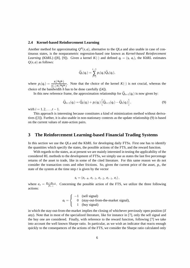
each time step. At the end of the trading period,t = T, the cumulative return is 510.86%. In figure2 we graphically report the results of the application of theQLa-based FTS to the real price seriesof Banca Intesa, withε = 5% andL = 5. At the end of the trading period,t = T, the cumulativereturn is 271.42%.

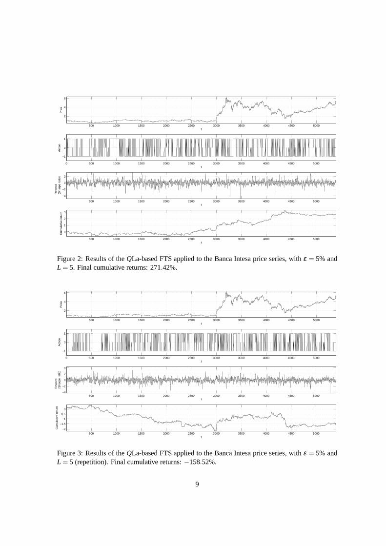
It is very important to note that at the beginning of the trading period,t = 0, the vector of theparameters used in the linear approximator,θk, is randomly initialized. Because of it, by repeatingsome times this latter application we observe a certain variability in the final cumulative return:−158.52%, 174.91%, −26.38% . . .. This shows that the influence of the random initializationheavily spreads overall the trading period instead to soften as time step increases. In figure 3 wegraphically report the results associated to the first of such repetition. To check the effects of thisrandom initialization, we repeated 1000 times the application of each of the investigated configura-tions. When the application was to the artificial time series, the series has been taken the same in allthe repetition. In table 1 we report some statistics concerning the final cumulative returns.

With reference to the KbRL, we obtain results similar to the one related to theQLa, althougha bit less performing. As exemplification: 1) in figure 4 we graphically report the results of theapplication of the KbRL-based FTS to the real price series ofBanca Intesa, withε = 5% andL =22 (at the end of the trading period,t = T, the cumulative return is 309.86%); 2) in figure 5 wegraphically report the results of the application of the KbRL-based FTS to the real price series ofFiat, with ε = 7.5% andL = 22 (at the end of the trading period,t = T, the cumulative return is135.47%). Note that for the KbRL there is not parameter vector to randomly initialize, but at thebeginning of the trading period,t = 0, it is necessary to randomly initialize a suitable set of state-

8

500 1000 1500 2000 2500 3000 3500 4000 4500 5000

2

4

6

Pric

e

t

0 500 1000 1500 2000 2500 3000 3500 4000 4500 5000

−1

0

1

Act

ion

t

500 1000 1500 2000 2500 3000 3500 4000 4500 5000

−4

−2

0

2

Rew

ard

(

Sha

rpe

ratio

)

t

500 1000 1500 2000 2500 3000 3500 4000 4500 5000

0

1

2

3

Cum

ulat

ive

retu

rn

t

Figure 2: Results of theQLa-based FTS applied to the Banca Intesa price series, withε = 5% andL = 5. Final cumulative returns: 271.42%.

500 1000 1500 2000 2500 3000 3500 4000 4500 5000

2

4

6

Pric

e

t

0 500 1000 1500 2000 2500 3000 3500 4000 4500 5000

−1

0

1

Act

ion

t

500 1000 1500 2000 2500 3000 3500 4000 4500 5000−4

−2

0

2

4

Rew

ard

(

Sha

rpe

ratio

)

t

500 1000 1500 2000 2500 3000 3500 4000 4500 5000

−2

−1.5

−1

−0.5

0

Cum

ulat

ive

retu

rn

t

Figure 3: Results of theQLa-based FTS applied to the Banca Intesa price series, withε = 5% andL = 5 (repetition). Final cumulative returns:−158.52%.

9

500 1000 1500 2000 2500 3000 3500 4000 4500 5000

2

4

6

Pric

e

t

0 500 1000 1500 2000 2500 3000 3500 4000 4500 5000

−1

0

1

Act

ion

t

500 1000 1500 2000 2500 3000 3500 4000 4500 5000

−0.5

0

0.5

Rew

ard

(

Sha

rpe

ratio

)

t

500 1000 1500 2000 2500 3000 3500 4000 4500 5000

0

1

2

3

Cum

ulat

ive

retu

rn

t

Figure 4: Results of the KbRL-based FTS applied to the Banca Intesa price series, withε = 5% andL = 22. Final cumulative returns: 309.86%.

action pairs ([8]). So, also in this approach one puts the question of the variability of the results. Asfor the QLa, for the KbRL too we repeated 1000 times the application ofeach of the investigatedconfigurations (see table 1 for some statistics about the final cumulative returns).

The main facts detectable from tables 1 are the following ones:

• Given the values of the means, most of the investigated configurations appears to be profitable,in fact the most of the means (88.89%) are positive. Further, theQLa approach generallyseems more performing than the KbRL one;

• Given the values of the standard deviations, the results of all the considered configurationsare characterized by a certain level of variability. In particular, such values emphasize that thequestion of the influence of the random initialization on theresults is mainly true for the realfinancial time series;

• Given the results, it appears that the value ofL has a significant impact on the performancesof the FTSs. In particular, with reference to the artificial time series, all the checked FTSconfigurations are better performing whenL = 5, whereas, with reference to both the realtime series, the most of the checked FTS configurations (91.67%) are better performing whenL = 22;

• Given the results, it appears that also the value ofε has a significant impact on the perfor-mances of the FTSs. In particular, although with reference to the artificial time series empir-

10

Approach ε L Statistics Artificial Banca Intesa Fiattime series time series time series

QLa 2.5% 5 µ 443.62% −3.77% 40.58%σ 37.83% 127.48% 139.35%

Conf. interval[369.48%,517.76%] [−253.53%,246.08%] [−232.55%,313.70%]QLa 2.5% 22 µ 307.03% 70.85% 101.21%

σ 43.02% 146.34% 144.27%Conf. interval[222.71%,391.35%] [−215.97%,357.68%] [−181.55%,383.98%]

QLa 5.0% 5 µ 472.02% 40.00% 91.26%σ 32.79% 139.09% 137.30%

Conf. interval[407.76%,536.29%] [−226.73%,306.73%] [−177.85%,360.37%]QLa 5.0% 22 µ 337.68% 92.92% 124.69%

σ 40.80% 149.28% 144.89%Conf. interval[257.71%,417.64%] [−199.66%,385.50%] [−159.29%,408.68%]

QLa 7.5% 5 µ 467.48% 49.15% 114.41%σ 31.11% 139.71% 142.42%

Conf. interval[406.50%,528.46%] [−224.67%,322.97%] [−164.73%,393.56%]QLa 7.5% 22 µ 339.04% 99.66% 133.81%

σ 39.60% 146.74% 147.53%Conf. interval[261.43%,416.66%] [−187.95%,387.28%] [−155.34%,422.96%]

KbRL 2.5% 5 µ 483.71% −26.16% 73.33%σ 60.10% 141.37% 144.00%

Conf. interval[365.91%,601.51%] [−303.25%,250.93%] [−208.90%,355.56%]KbRL 2.5% 22 µ 237.64% 15.90% 75.37%

σ 63.55% 159.92% 131.08%Conf. interval[113.09%,362.20%] [−297.54%,329.34%] [−181.55%,332.28%]

KbRL 5.0% 5 µ 435.42% −7.99% 77.32%σ 41.13% 131.26% 130.42%

Conf. interval[354.81%,516.02%] [−265.26%,249.28%] [−178.30%,332.95%]KbRL 5.0% 22 µ 216.61% 13.20% 71.98%

σ 49.98% 153.34% 136.04%Conf. interval[118.64%,314.58%] [−287.34%,313.74%] [−194.66%,338.61%]

KbRL 7.5% 5 µ 401.76% −0.63% 67.55%σ 39.80% 130.40% 128.00%

Conf. interval[323.75%,479.77%] [−256.23%,254.96%] [−183.33%,318.42%]KbRL 7.5% 22 µ 197.78% 35.36% 74.82%

σ 42.55% 143.51% 132.06%Conf. interval[114.38%,281.18%] [−245.91%,316.63%] [−184.02%,333.65%]

Table 1: Some statistics about the final cumulative returns.

11

500 1000 1500 2000 2500 3000 3500 4000 4500 5000

10

20

30

40

Pric

e

t

0 500 1000 1500 2000 2500 3000 3500 4000 4500 5000

−1

0

1

Act

ion

t

500 1000 1500 2000 2500 3000 3500 4000 4500 5000

−0.5

0

0.5

Rew

ard

(

Sha

rpe

ratio

)

t

500 1000 1500 2000 2500 3000 3500 4000 4500 50000

0.5

1

1.5

Cum

ulat

ive

retu

rn

t

Figure 5: Results of the KbRL-based FTS applied to the Fiat price series, withε = 7.5% andL= 22.Final cumulative returns: 135.47%.

ical regularities does not appear, with reference to both the real time series, the most of thechecked FTS configurations (75.00%) are better performing whenε = 7.5%.

4 Some concluding remarks

In this paper we have developed and applied some original automatic FTSs based on differentlyconfigured RL algorithms. Here we have presented the resultscoming out from the current phaseof our research on this topic. Of course, many questions haveagain to be explored. In particular:

• The choice of the last five percentage returns as states is a naive choice. Now we are beginningto work to specify some new indicators to use as states (in thefirst experimentations they haveprovided interesting results);

• As known, the Sharpe ratio as performance measure suffers several limits. Currently, asreward function we are considering alternative and more realistic performance measures;

• The management of the learning rate,α , we have used here is appropriate for stationary sys-tems. But generally financial markets are non-stationary. Because of that, we are beginning towork to develop methods for the dynamic management of the learning rate in non-stationarycontexts;

12

• In order to deepen the valuation about the capabilities of our FTSs, we wish to apply them tomore and more financial price series coming from different markets;

• Finally, when all the previous questions will be explored, transaction costs and other frictionswill be considered.

Acknowledgements

The authors wish to thank the Department of Economics of the Ca’ Foscari University of Venicefor the support received within the research projectMachine Learning adattativo per la gestionedinamica di portafogli finanziari[Adaptative Machine Learning for the dynamic management offinancial portfolios]).

References

[1] Barto A.G., Sutton R.S. (1998),Reinforcement Learning: An Introduction. Adaptive Compu-tation and Machine Learning. The MIT Press.

[2] Bertsekas D.P., Tsitsiklis J.N. (1996),Neuro-Dynamic Programming. Athena Scientific.

[3] Brent R.P. (1973),Algorithms for Minimization without Derivatives. Prentice-Hall.

[4] Bosq D. (1996),Nonparametric Statistics for Stochastic Processes. Estimation and Prediction[Lecture Notes in Statistics, vol. 110]. Springer-Verlag.

[5] Gold C. (2003), FX trading via recurrent Reinforcement Learning,Proceedings of the IEEEInternational Conference on Computational Intelligence in Financial Engineering, 363-370.

[6] Moody J., Wu L., Liao Y., Saffel M. (1998), Performance functions and Reinforcement Learn-ing for trading systems and portfolios,Journal of Forecasting, 17, 441-470.

[7] Moody J., Saffel M. (2001), Learning to trade via Direct Reinforcement,IEEE Transactionson Neural Network, 12, 875-889.

[8] Ormonet D. (2002), Kernel-Based Reinforcement Learning, Machine Learning, 49, 161-178.

[9] Smart W.D., Kaelbling L.P. (2000), Practical Reinforcement Learning in continuous spaces,Proceedings of the 17th International Conference on Machine Learning, 903-910.

13