ISSN 2282-6483

Product Differentiation with

Multiple Qualities

Francesca Barigozzi

Ching-to Albert Ma

Quaderni - Working Paper DSE N°1075

Product Di¤erentiation with Multiple Qualities

Francesca Barigozzi Ching-to Albert Ma

Department of Economics Department of EconomicsUniversity of Bologna Boston University

francesca.barigozzi@unibo.it ma@bu.edu

August 30, 2016

Abstract

We study subgame-perfect equilibria of the classical quality-price, multistage game of vertical productdi¤erentiation. Each �rm can choose the levels of an arbitrary number of qualities. Consumers�valuationsare drawn from independent and general distributions. The unit cost of production is increasing and convexin qualities. We characterize equilibrium prices, and the equilibrium e¤ects of qualities on the rival�s pricein the general model. We present necessary and su¢ cient conditions for equilibrium di¤erentiation in any ofthe qualities.

Keywords: multidimensional product di¤erentiation, quality and price competition

JEL: D43, L13

Acknowledgement: For their comments, we thank Sofronis Clerides, Bard Harstad, Henry Mak, KjetilStoresletten and seminar participants at Boston University, the University of Oslo, and the 14th InternationalIndustrial Organization Conference in Philadelphia.

1 Introduction

Firms using di¤erentiated products to soften intense Bertrand price competition is a basic principle in

industrial organization. Following Hotelling (1929), D�Aspremont, Gabszewicz and Thisse (1979) clarify

theoretical issues and solve the basic horizontal di¤erentiation model. Gabszewicz and Thisse (1979), and

Shaked and Sutton (1982, 1983) work out equilibria of the basic vertical di¤erentiation model.

The standard model of horizontal-vertical product di¤erentiation is the following multistage game between

two �rms: in Stage 1, �rms choose product attributes, in Stage 2, �rms choose prices, and then consumers

pick a �rm to purchase from. In the literature, models have seldom gone beyond two possible qualities, have

assumed that consumers�quality valuations are uniformly distributed, and have let production or mismatch

costs be nonexistent, linear, or quadratic. We make none of these assumptions. In this paper, each of two

�rms produces goods with an arbitrary number of quality attributes. Consumers�valuations on each quality

follow a general distribution. A �rm�s unit production cost is an increasing and convex function of qualities.

In this general environment, we fully characterize subgame-perfect equilibria of the standard di¤erentiation

model.

Using the uniform quality-valuation distribution and the separable cost assumptions, researchers have

managed to solve for equilibrium prices explicitly as functions of qualities. Equilibrium qualities then can

be characterized. What has emerged in the literature are a few classes of equilibria with largest or smallest

di¤erences in equilibrium qualities (see the literature review in the following subsection). Indeed, in equi-

librium �rms may successfully di¤erentiate their products in some qualities, but may fail to do so in others.

Obviously, tractability versus generality is the challenge that has been posed by the literature. How robust

are maximal or minimal di¤erentiation results? To what extent are they driven by these assumptions?

In this paper we solve the tractability-generality dilemma. For the quality-price, multistage game, we

completely characterize subgame-perfect equilibria. First, we �nd out how qualities change equilibrium

prices� without solving for the equilibrium prices explicitly in terms of qualities. In other words, we do

not need the usual assumptions in order to compute equilibrium prices explicitly. Second, we identify two

separate e¤ects for the characterization of equilibrium qualities. The �rst is what we call the price-reaction

1

e¤ect, which is how a �rm�s quality in Stage 1 a¤ects the rival �rm�s price in Stage 2. The second is what

we call the Spence e¤ect (because it is originally exposited in Spence (1975); see footnote 7). For maximum

pro�t, a �rm chooses a quality which is e¢ cient for the consumer who is just indi¤erent between buying

from the �rm and its rival.

Consumers must buy from one of the two �rms, so �rms share the same set of indi¤erent consumers. The

Spence e¤ect says that each �rm should choose those qualities that are e¢ cient for the equilibrium set of

indi¤erent consumers. The Spence e¤ect alone is a motivation for minimal product di¤erentiation: for each

quality, �rms should choose the same level. But there is a second e¤ect at work.

In the standard multistage game, prices are strategic complements. In Stage 1, each �rm would like to use

its qualities to induce the rival to choose a higher price in Stage 2. The rival �rm�s strategic consideration,

however, is exactly the same. Hence, the two �rms engage in a race. For each quality, the relative strength of

the price-reaction e¤ect determines which �rm will, in equilibrium, choose a higher quality than its rival. For

general distributions of quality valuations and a general cost function, it is entirely possible for the relative

strength to vary across di¤erent qualities. The price-reaction e¤ect implies that �rms may di¤erentiate their

products in many ways. Largest or smallest di¤erences in equilibrium qualities are not robust. Instead, we

provide a full characterization of how equilibrium qualities may di¤er between �rms.

Our results say that �rms choosing the same level of a quality holds under very restrictive conditions: cost

is separable across quality attributes together with consumers�quality valuations being uniformly distributed

(see Corollary 3 below). However, these have been the exact assumptions used in the literature. One casually

observes that quality attributes across products are never exactly the same. Thus, �rms that produce �high-

end�products will still di¤erentiate� if only in small details of their product qualities. For example, BMW

and Lexus are companies that di¤erentiate even in the high qualities of their cars. All BMW and Lexus

cars are high-quality automobiles, but the common consensus is that BMW has a higher �performance�

quality than Lexus, but the opposite is true when it comes to the �comfort�quality. However, any car by

BMW or Lexus will be a better performer and more comfortable than any car by Yugo. In fact, in the

automobile (and most other) markets, it is impossible to �nd products that have identical quality attributes.

2

These observations are consistent with the general tenet of product di¤erentiation, but inconsistent with

assumptions of uniform quality-valuation distribution and separable cost functions.

What is behind our solution to the tractability-generality dilemma? Our key innovation is to show that

solving for the equilibrium prices as functions of qualities is equivalent to solving a single integral equation.

The solution to the integral equation yields the equilibrium set of indi¤erent consumers, and hence the �rms�

demands. We obtain this solution as an implicit function of the model primitives. Then a �rm�s equilibrium

price can be expressed explicitly in terms of qualities, through the solution of the integral equation. In other

words, we dispense with the need for explicit computation of equilibrium prices, which would require explicit

speci�cation of the model primitives, a common research strategy in the literature. Judicious analysis of

mutual quality best responses, given qualities�impact on equilibrium prices, yields the fundamental price-

reaction and Spence e¤ects. For many examples, the integral equation does admit an explicit solution (that

will be demonstrated later).

We use a vertical di¤erentiation model, but Cremer and Thisse (1991) show that for the usual model

speci�cation, the Hotelling, horizontal di¤erentiation model is a special case of the vertical di¤erentiation

model. The intuition is simply that �rms�demand functions in a Hotelling model can be directly translated

to the demand functions in a vertical, quality model. Cremer and Thisse (1991) state the result for a single

location or quality dimension, but their result extends straightforwardly to an arbitrary number of such

dimensions. (A model with a combination of horizontal and vertical dimensions can also be translated to

a model with only vertical dimensions.) Hence our results in this paper apply to horizontal-di¤erentiation

models. In particular, our method of solving for equilibrium prices is valid for Hotelling models.1

We continue with a subsection on the literature. In Section 2, we de�ne consumers�preferences and �rms�

technology. Then we set up the quality-price, multistage game. Section 3 is divided into four subsections.

In Subsection 3.1, we characterize subgame-perfect equilibrium prices. Lemma 1 presents the solution of the

integral equation, the key step in expressing equilibrium prices as functions of qualities. In Subsection 3.2,

1Di¤erences between horizontal and vertial models may also be due to speci�cation of the strategy sets. Here, weallow qualities to take any positive values; in location models, �rms�positions may not vary as much. See also thediscussions following Corollary 3.

3

we characterize how prices change with qualities. In Subsection 3.3, we characterize equilibrium qualities,

and establish the price-reaction and Spence e¤ects. Subsection 3.4 presents a number of implications. We

specialize our model by adopting common assumptions (uniform quality-valuation distribution and separable

cost function), and draw connections between earlier results and ours. A number of examples are studied in

Section 4. These examples illustrate how our general results can be used. The last section contains some

concluding remarks. Proofs of results are in Appendix A, and some steps for computation for Subsection 4.3

are in Appendix B.

1.1 Literature review

The modern literature on product di¤erentiation and competition begins with D�Aspremont, Gabszewicz and

Thisse (1979), Gabszewicz and Thisse (1979) and Shaked and Sutton (1982, 1983). In the past few decades,

the principle of product di¤erentiation relaxing price competition has been stated in texts of industrial

organization at all levels: Tirole (1988), Anderson, De Palma, and Thisse (1992), and Belle�amme and

Peitz (2010) for graduate level, as well as Cabral (2000), Carlton and Perlo¤ (2005), and Pepall, Richards,

and Norman (2014). Many researchers use the basic horizontal and vertical di¤erentiation models as their

investigation workhorse.

The research here focuses on equilibrium di¤erentiation. In both horizontal and vertical models, a com-

mon theme has been to solve for subgame-perfect equilibria in the quality-price, multistage game in various

environments.2 First, earlier papers have looked at single or multiple horizontal and vertical dimensions of

consumer preferences. Second, most papers have adopted the assumption that these preferences are uni-

formly distributed. Third, most papers in the horizontal model have used a quadratic consumer mismatch

disutility function, whereas those in the vertical model have assumed that the unit production cost is either

independent of, or linear in quality.

Single dimension of preferences

Anderson, Goeree and Ramer (1997) study equilibrium existence and characterization in a single-dimension

2As we have already mentioned, Cremer and Thisse (1991) (following on a suggestion by Champsaur and Rochet(1989)) show that horizontal-location models are special cases of vertical models.

4

horizontal model. They use a general consumer preference distribution but quadratic mismatch disutility.

Our multidimensional vertical model can be recast into the single-dimension model in Anderson, Goeree

and Ramer, and we will demonstrate that in Subsection 4.2. A few other papers have adopted nonuniform

distributions on consumer locations. Neven (1986) shows that �rms tend to locate inside the market when

consumers�densities are higher near the center. Tabuchi and Thisse (1995) assume a triangular distribution

and �nd that there is no symmetric location equilibria but that asymmetric location equilibria exist. Yurko

(2010) uses a vertical model for studying entry decisions, but her results are based on numerical simula-

tions. Benassi, Chirco, and Colombo (2006) allow consumers the nonpurchase option. They relate various

trapezoidal valuation distributions to degrees of equilibrium quality di¤erentiation. Finally, Loertscher and

Muehlheusser (2011) consider entry in location games without price competition. They study equilibria

under the uniform and some nonuniform consumer-location distributions.

Multiple dimensions of vertical preferences

A few papers have studied vertical models with two dimensions. These are Vandenbosch and Weinberg

(1995), Lauga and Ofek (2011), and Garella and Lambertini (2014). All three papers use the uniform

valuation distribution. In Subsection 3.4, we will present the relationship between our results here to those

in these papers. Here, we note that these papers have assumed zero production cost, or unit cost that is

linear or discontinuous in quality. By contrast we use a strictly convex quality cost function.

Multiple dimensions of horizontal preferences

For horizontal models with multiple dimensions, the key paper is Irmen and Thisse (1998), who set up

an N dimensional model to derive what they call �Max-Min-...Min�equilibria. We will relate our results to

those in Irmen and Thisse in Subsection 3.4, right after Corollary 4. Tabuchi (1994) and Vendorp and Majeed

(1995) are special cases of Irmen and Thisse (1998) at N = 2. Ansari, Economides, and Steckel (1998) study

two and three dimensional Hotelling models, and derive similar results as in Irmen and Thisse (1998). All

assume that consumers�locations are uniformly distributed, and that the mismatch disutility is Euclidean

and therefore separable. We are unaware of any paper in the multidimensional horizontal literature that

adopts general consumer preferences distributions, or general, nonseparable mismatch disutility.

5

Finally, Degryse and Irmen (2001) use a model with both horizontal and vertical di¤erentiation. For the

horizontal dimension, consumer locations are uniformly distributed. For the vertical dimension, consumers

have the same valuation (as in the model in Garella and Lambertini (2014)). However, the mismatch disutility

depends also on quality, which corresponds to the case of a nonseparable mismatch disutility or quality cost

function. This can be thought of as a special case of the model here; see Subsection 4.2.

2 The Model

We begin with consumers and their preferences. Then we present two identical �rms. Finally, we de�ne

demands, pro�ts, and the extensive form of quality-price competition.

2.1 Consumers and preferences for qualities

There is a set of consumers, with total mass normalized at 1. Each consumer would like to buy one unit of

a good, which has N � 2 quality attributes. A good is de�ned by a vector of qualities (q1; q2 :::; qN ) 2 <N+ ,

where qi is the level of the ith quality, i = 1; 2; :::; N . Sometimes, we use the term quality qi to mean the

level of quality attribute i.

A consumer�s preferences on goods are described by his quality valuations, represented by the vector

(v1; :::; vi; :::; vN ) 2QNi=1[vi; vi] � <N++. The valuation on quality qi is vi, which varies in a bounded, and

strictly positive interval. If a consumer with valuation vector (v1; :::; vi; :::; vN ) � v buys a good with qualities

(q1; q2 :::; qN ) � q at price p, his utility is v1q1+v2q2+ :::+vNqN �p. (We may sometimes call this consumer

(v1; :::; vN ) or simply consumer v.) The quasi-linear utility function is commonly adopted in the literature

(see such standard texts as Tirole (1988) and Belle�amme and Peitz (2010))

Consumers�heterogeneous preferences on qualities are modeled by letting the valuation vector be random.

We use the standard independence distribution assumption: the valuation vi follows the distribution function

Fi with the corresponding density fi, i = 1; :::; N , and these distributions are all independent. Each density

is assumed to be di¤erentiable (almost everywhere) and logconcave. The logconcavity of fi implies that the

6

joint density of (v1; :::; vi; :::; vN ) � v is logconcave,3 and it guarantees that pro�t functions, to be de�ned

below, are quasi-concave (see Proposition 4 in Caplin and Nalebu¤ 1991, p39).

2.2 Firms and extensive form

There are two �rms and they have access to the same technology. If a �rm produces a good at quality vector

(q1; q2 :::; qN ) � q, the per-unit production cost is C(q). There is no �xed cost, so if a �rm produces D units

of the good at quality q, its total cost is D multiplied by C(q). We assume that the per-unit quality cost

function C : RN+ ! R+ is strictly increasing and strictly convex. We also assume that C is continuous and

di¤erentiable, and satis�es the usual Inada conditions: limq!0 C(q) = limq!0dC(q) = 0 (where 0 stands for

either the number zero or an N -vector of all zeros), and that limq!1 C(q) = limq!0dC(q) = 1 (again 1

stands for in�nity or an N -vector of in�nities).4 If a �rm sells D units of the good with quality vector q at

price p, its pro�t is D � [p� C(q)].

The two �rms are called Firm A and Firm B. We use the notation q for Firm A�s vector of qualities

(q1; q2; ::::::qN ) � q. We use the notation r for Firm B�s vector of qualities (r1; r2; ::::::rN ) � r. Hence, when

we say quality qi, it indicates the level of Firm A�s quality attribute i, whereas when we say quality ri, it

indicates the level of Firm B�s quality attribute i. Let Firm A�s price be pA, and Firm B�s price be pB . We

use the notation p for the price vector (pA; pB).

Given the two �rm�s quality choices, consumer v = (v1; ::; vN ) obtains utilities v1q1+v2q2+:::+vNqN�pA

or v1r1 + v2r2 + :::+ vNrN � pB from Firm A or Firm B, respectively. Consumer v purchases from Firm A

if and only if v � q � pA > v � r � pB . If the consumer is indi¤erent because v � q � pA = v � r � pB , he picks

a �rm to buy from with probability 0:5. For given quality vectors and prices, the demands for Firm A and

Firm B are, respectively,Z� �ZZ

v�q�pA�v�r�pB

dF1dF2 � �dFN andZ� �ZZ

v�q�pA�v�r�pB

dF1dF2 � �dFN :

3Because of independence, the joint density of (v1; :::; vi; :::; vN ) isQNi=1 fi. Hence, ln

Qfi =

Pln fi. Because

ln fi is concave, so isPln fi.

4We have used a general cost function, whereas papers in the extant literature adopt various more restrictiveassumptions. Popular simpli�cations include C being separable in qualities, C being linear, or even identically zero.More discussions are in Subsection 3.4.

7

The two �rms�pro�ts are8<:Z� �ZZ

v�q�pA�v�r�pB

dF1dF2 � �dFN

9=; [pA � C(q)] � �A(pA; pB ; q; r) (1)

8<:Z� �ZZ

v�q�pA�v�r�pB

dF1dF2 � �dFN

9=; [pB � C(r)] � �B(pA; pB ; q; r): (2)

In case q = r, and pA = pB , each �rm sells to one half of the mass of consumers.

We study subgame-perfect equilibria of the standard multistage game of quality-price competition:

Stage 0: Consumers valuations are drawn from respective distributions.

Stage 1: Firm A and Firm B simultaneously choose their product qualities q and r, respectively.

Stage 2: Firm A and Firm B simultaneously choose their product prices. Then each consumer picks a �rm

to buy from.

3 Equilibrium product di¤erentiation

We begin with the subgame in Stage 2, de�ned by a pair of quality vectors chosen by �rms in Stage 1.

Let Firm A�s qualities be (q1; q2; :::; qN ) � q, and let Firm B�s qualities be (r1; r2; :::rN ) � r. If Firm

A�s and Firm B�s prices are pA and pB , respectively, consumer v = (v1; :::; vN ) now buys from Firm A if

v � q � pA > v � r � pB . The set of consumers who are indi¤erent between buying from Firm A and Firm B

is given by the equation v1q1 + :::+ vNqN � pA = v1r1 + :::+ vNqN � pB . For q1 6= r1 we solve for v1 in this

equation to de�ne the following function:

ev1(v�1; p; q; r) � pB � pAr1 � q1

�NPk=2

vkrk � qkr1 � q1

; (3)

where v�1 = (v2; :::; vN ) is the vector of valuations of the second to the last quality attributes. The vector

(ev1(v�1; p; q; r); v2; :::; vN ) � (ev1(v�1; p; q; r); v�1) describes all consumers who are indi¤erent between buyingfrom the two �rms.

The function ev1 in (3) is linear in the valuations, and this is an important property from the quasi-linear

consumer utility function. The function is illustrated in Figure 1 for the case of two qualities (N = 2).

8

Figure 1: Consumers�choices given prices and qualities

There, we have the valuation v1 on the vertical axis, and the valuation v2 on the horizontal axis. For this

illustration, we have set (q1; q2) < (r1; r2) and pA < pB . The function ev1 is the negatively sloped straightline with the formula ev1(v2; p; q; r) = pB � pA

r1 � q1�v2

r2 � q2r1 � q1

. Prices a¤ect only the intercept, whereas qualities

a¤ect both the intercept and the slope.

We further consider the case of q1 < r1. Consumer (v01; v2; :::vN ) buys from Firm B if and only if

v01 > ev1(v�1; p; q; r). In other words, if quality r1 is higher than quality q1, Firm B�s product is more

attractive to a consumer with a higher valuation v1. In Figure 1, the set of consumers who buy from Firm

B consists of those above ev1. Hence, we reformulate the �rms�demands as:Firm A Firm BZ vN

vN

:::

Z v2

v2

Z ev1v1

v�q�pA�v�r�pB

�Ni=1dFi(vi)

=

Z vN

vN

:::

Z v2

v2

F1(ev1(v�1; p; q; r))�Nk=2dFk(vk)

Z vN

vN

:::

Z v2

v2

Z v1

ev1v�q�pA�v�r�pB

�Ni=1dFi(vi)

=

Z vN

vN

:::

Z v2

v2

[1� F1(ev1(v�1; p; q; r))]�Nk=2dFk(vk):For some values of q, r, and prices pA and pB , as v�1 varies over its ranges, the value of the formula in (3)

may be outside the support [v1; v1]. We can formally include these possibilities by extending the valuation

support over the entire real line, but set f1(x) = 0 whenever x lies outside the support [v1; v1]. For easier

exposition, we will stick with the current notation.

9

We use the following shorthand to simplify the notation:

Zv�1

stands forZ vN

vN

:::

Z v2

v2

and dF�1 stands for �Nk=2dFk(vk):

Pro�ts of Firms A and B are, respectively:

�A (pA; pB ; q; r) =

Zv�1

F1(ev1(v�1; p; q; r))dF�1 � [pA � C(q)] (4)

�B (pA; pB ; q; r) =

Zv�1

[1� F1(ev1(v�1; p; q; r))]dF�1 � [pB � C(r)] : (5)

3.1 Subgame-perfect equilibrium prices

A subgame in Stage 2 is de�ned by the �rms�qualities. Let Firm A�s quality vector be q and Firm B�s

quality vector be r, so we identify a subgame in Stage 2 by quality vectors (q; r). It is clear that if q = r,

the equilibrium in Stage 2 is the standard Bertrand equilibrium so each �rm will charge its unit production

cost: pA = pB = C(q) = C(r).

We now turn to subgames in which q 6= r. By a permutation of quality indexes and interchanging

the �rms� indexes if necessary, we let q1 < r1. A price equilibrium in subgame (q; r) is a pair of prices

(p�A; p�B) that are best responses: p

�A = argmaxpA �A(pA; p

�B ; q; r) and p

�B = argmaxpB �B(p

�A; pB ; q; r), where

the pro�t functions are de�ned by (4) and (5). The existence of a price equilibrium follows from Caplin

and Nalebu¤ (1991). Furthermore, because of the logconcavity assumption on the densities, a �rm�s pro�t

function is quasi-concave in its own price.

As we will show, the characterization of equilibrium prices boils down to the properties of the solution

of an integral equation. We begin with di¤erentiating the pro�t functions with respect to prices:

@�A@pA

=

Zv�1

F1(ev1(v�1; p; q; r))dF�1 � Zv�1

f1(ev1(v�1; p; q; r))dF�1 �pA � C(q)r1 � q1

�

@�B@pB

=

Zv�1

[1� F1(ev1(v�1; p; q; r))]dF�1 � Zv�1

f1(ev1(v�1; p; q; r))dF�1 �pB � C(r)r1 � q1

�;

where we have used the derivatives of ev1(v�1; p; q; r) in (3) with respect to pA and pB .

10

The equilibrium prices (p�A; p�B) � p� satisfy the �rst-order conditions:

p�A � C(q) =

Zv�1

F1(ev1(v�1; p�; q; r))dF�1Zv�1

f1(ev1(v�1; p�; q; r))dF�1 (r1 � q1) (6)

p�B � C(r) =

Zv�1

[1� F1(ev1(v�1; p�; q; r))]dF�1Zv�1

f1(ev1(v�1; p�; q; r))dF�1 (r1 � q1) (7)

where

ev1(v�1; p�; q; r) = p�B � p�Ar1 � q1

�NPk=2

vkrk � qkr1 � q1

; vk 2 [vk; vk]; k = 2; :::; N: (8)

Equations (6) and (7) say that the price-cost margins follow the usual inverse elasticity rule, a standard

result.5 The complication is that (8) sets up a function ev1 that depends on N � 1 continuous variables vk,

k = 2; ::; N , and the quality vector (q; r), and this is to be determined simultaneously with the prices in (6)

and (7).

Let p� = (p�A; p�B) be the subgame-perfect equilibrium prices in Stage 2 in subgame (q; r). The equilibrium

prices are functions of the quality vector, so we write them as p�(q; r). Let ev1(v�1; p� (q; r) ; q; r) be thesolution of (8) at the subgame-perfect equilibrium. Now we de�ne ev�1(v�1; q; r) � ev1(v�1; p� (q; r) ; q; r),which describes the set of consumers who are indi¤erent between buying from Firm A and Firm B in an

equilibrium in subgame (q; r). By substituting the equilibrium prices (6) and (7) into ev1(v�1; p� (q; r) ; q; r)in (8) above, we have:

ev�1(v�1; q; r) =Zv�1

[1� 2F1(ev�1(v�1; q; r))]dF�1Zv�1

f1(ev�1(v�1; q; r))dF�1 +C(r)� C(q)r1 � q1

�NPk=2

vkrk � qkr1 � q1

: (9)

This is an integral equation in ev�1 , and the solution holds the key to the characterization of the priceequilibrium. Indeed, we have decomposed the system in (6), (7) and (8) into two systems: a single integral

equation (9), and those two equations (6) and (7). The integral equation (9) is independent of prices. Using

the solution to (9), we can then proceed to solve for the equilibrium prices in (6) and (7). We are unaware

5 If we divide (6) by p�A, it can easily be seen that the right-hand side is the inverse elasticity of demand, which is

obtained from the demandZv�1

F1(ev1(v�1; p; q; r))dF�1:

11

that any paper in the extant literature of multiple qualities has decomposed the equilibrium prices and

demand characterization in this fashion. Yet, using this decomposition, we can characterize the functional

relationship between quality and equilibrium prices.

Lemma 1 The solution of the integral equation (9) takes the form ev�1(v�1; q; r) = �(q; r)�PNk=2 vk�k(q; r),

for vk 2 [vk; vk]; k = 2; :::; N , where the functions � and �k are de�ned by

�(q; r) =

Zv�1

h1� 2F1(�(q; r)�

PNk=2 vk�k(q; r))

idF�1Z

v�1

f1(�(q; r)�PN

k=2 vk�k(q; r))dF�1+C(r)� C(q)r1 � q1

(10)

�k(q; r) =rk � qkr1 � q1

; k = 2; :::; N: (11)

The solution in Lemma 1, ev�1(v�1; q; r) = �(q; r)�v�1���1(q; r), describes the equilibrium set of indi¤erentconsumers in subgame (q; r) where we have used the common abbreviation ��1(q; r) � (�2(q; r); �3(q; r);

:::; �N (q; r)). From (6) and (7), a �rm�s qualities a¤ect equilibrium prices of both �rms. In turn, when

equilibrium prices change, the set of indi¤erent consumers change accordingly. The composition of the

quality e¤ect on equilibrium prices, and then the e¤ect of equilibrium prices on the equilibrium set of

indi¤erent consumers is the solution in Lemma 1. The equilibrium set of indi¤erent consumers takes the

linear form, so the intercept � and all the slopes �k, k = 2; :::; N are functions of the qualities.

Lemma 1 is a remarkable result. First, the solution of the integral equation (9) takes a manageable

form: it consists of one implicit function �(q; r) in (10) and N � 1 explicit (and simple) functions �k(q; r),

k = 2; :::; N , in (11). In other words, for any �xed number of quality attributes, there is only one implicit

function like the one in (10) to handle. Also, the equilibrium prices boil down to solving for the solutions of

just three equations. From the discussion above and by substituting the expressions for (10) and (11) to the

right-hand side of (6) and (7), we can state the following proposition (proof omitted):

12

Proposition 1 In subgame (q; r), equilibrium prices are the solution of p�A in (12) and p�B in (13):

p�A � C(q) =

Zv�1

F1(�(q; r)� v�1 � ��1(q; r))dF�1Zv�1

f1(�(q; r)� v�1 � ��1(q; r))dF�1(r1 � q1) (12)

p�B � C(r) =

Zv�1

�1� F1(�(q; r)� v�1 � ��1(q; r))

�dF�1Z

v�1

f1(�(q; r)� v�1 � ��1(q; r))dF�1(r1 � q1); (13)

with �(q; r) implicitly de�ned by (10), and �k(q; r) =rk � qkr1 � q1

; k = 2; :::; N:

The importance of Proposition 1 is this. The equilibrium price p�A is given by (12), an explicit function

of qualities. Thus, a direct di¤erentiation of p�A with respect to qualities yields all the relevant information

of how any of Firm B�s quality choice changes Firm A�s equilibrium price. The same applies to p�B and (13).

The common link between p�A in (12) and p�B in (13) is the implicit function (10), the explicit functions (11),

and the distributions of quality valuations. How do qualities change prices?

3.2 Qualities and equilibrium prices

We begin with writing equilibrium prices p�A in (12) and p�B in (13) as

p�A � C(q)r1 � q1

= G��; ��1

�and

p�B � C(r)r1 � q1

= H��; ��1

�,

where the functions: G��; ��1

�: <N ! <, and H

��; ��1

�: <N ! < are de�ned by

G��; ��1

��

Zv�1

F1(�� v�1 � ��1)dF�1Zv�1

f1(�� v�1 � ��1)dF�1(14)

H��; ��1

��

Zv�1

�1� F1(�� v�1 � ��1)

�dF�1Z

v�1

f1(�� v�1 � ��1)dF�1: (15)

The functions G and H are the �rms�price-cost markups per unit of quality di¤erence. Working directly

with these price-cost markups has a¤orded us tractability.6 However, our �nal results will be expressed in

6For a model with only one quality attribute, the markups are the reverse hazard rate, F=f , and the hazard rate(1� F )=f , where F and f are the distribution and density functions of the quality valuation.

13

terms of the primitives of the model: the density and distribution functions, fi and Fi, i = 1; 2:::; N and

the cost function C. We have omitted the quality arguments in � and ��1 � (�2; :::; �N ) for a shorter set

of notation here. The numerators of G��; ��1

�and H

��; ��1

�are, respectively, Firm A�s and Firm B�s

demands. The common denominator is the total density of the set of indi¤erent consumers. Indi¤erent

consumers are those with valuations satisfying v � q � pA = v � r � pB . Hence, the total density of this set isRv�q�pA=v�r�pB

QNi=1dFi(vi) =

Rv�1

f1(ev�1)dF�1.Recall that �(q; r) and �k(q; r) are given by Lemma 1. Hence, we can directly di¤erentiate p

�A with

respect to Firm B�s qualities, and di¤erentiate p�B with respect Firm A�s qualities, and we call these the

price-reaction e¤ects:

@p�A@r1

= (r1 � q1)@G��; ��1

�@r1

= G��; ��1

�+ (r1 � q1)

"@G

@�

@�

@r1+

NXk=2

@G

@�k

@�k@r1

#(16)

@p�B@q1

= (r1 � q1)@H

��; ��1

�@q1

= �H��; ��1

�+ (r1 � q1)

"@H

@�

@�

@q1+

NXk=2

@H

@�k

@�k@q1

#; (17)

and

@p�A@rj

= (r1 � q1)@G��; ��1

�@rj

= (r1 � q1)�@G

@�

@�

@rj+@G

@�j

@�j@rj

�; j = 2; :::; N (18)

@p�B@qj

= (r1 � q1)@H

��; ��1

�@qj

= (r1 � q1)�@H

@�

@�

@qj+@H

@�j

@�j@qj

�; j = 2; :::; N: (19)

Because we label a di¤erentiated quality attribute as the �rst attribute (q1 < r1), there is a slight di¤erence

between the form of price-reaction e¤ects of the �rst quality and the other qualities. (With all the arguments

displayed, the function G is G(�; �2; :::; �N ) = G��; r2�q2r1�q1 ; :::;

rN�qNr1�q1

�. Similarly, for the function H. The

arguments �2; :::; �N in G and H include r1 and q1, so if we partially di¤erentiate G or H with respect to

r1 and q1, we get the summation terms in (16) and (17). However, for j = 2; :::; N , rj and qj are only in the

argument �j in G and H. When we partially di¤erentiate G or H with respect to rj or qj , we only get the

simpler expressions in (18) and (19).)

The expression in (18) displays a composition of two e¤ects. The �rst is how qualities change the

intercept � and slopes ��1 of the equation that determines the equilibrium set of indi¤erent consumers

14

ev�1(v�1; q; r) = �(q; r)� v�1 � ��1(q; r); these are the terms @�@rj , @�j@rj,@�

@qj, and

@�j@qj

. The second is how the

equilibrium set of consumers change the price-cost markups G��; ��1

�and H

��; ��1

�; these are the terms

@G

@�,@G

@�j,@H

@�and

@H

@�j, j = 2; :::; N .

We �rst present how the sum in markups varies with the equilibrium set of indi¤erent consumers. Then

we can obtain how the sum varies with the intercept and slope of the equations for the set of indi¤erent

consumers.

Lemma 2 In any subgame (q; r), the sum of the proportional changes in the �rms� equilibrium price-cost

markups and the proportional change in the total density of the equilibrium set of indi¤erent consumers must

vanish:

d ln[G(�; ��1) +H(�; ��1)] + d lnZv�1

f1(�� v�1 � ��1)dF�1 = 0. (20)

It follows that the sum of the partial derivatives of G(�; ��1) and H(�; ��1) with respect to � and �j,

j = 2; :::; N are

@G

@�+@H

@�=�

Zv�1

f 01(�� v�1 � ��1)dF�1 Zv�1

f1(�� v�1 � ��1)dF�1

!2 (21)

@G

@�j+@H

@�j=

Zv�1

f 01(�� v�1 � ��1)vjdF�1 Zv�1

f1(�� v�1 � ��1)dF�1

!2 : (22)

Lemma 2 follows from the de�nitions of G and H and from straightforward di¤erentiation. From the

de�nitions (14) and (15), we have:

G+H =1Z

v�1

f1(�� v�1 � ��1)dF�1: (23)

At each subgame (q; r) the market is always covered, the total price-cost markup is always equal to the

reciprocal of the total density of equilibrium set of indi¤erent consumes. Hence, equation (20) follows. If

somehow the intercept of the equilibrium set of consumers (�) increases, the sum of �rms�price-cost markups

15

will be in (21). Similarly, if the jth slope of the equilibrium set of indi¤erent consumers (�j) increases, the

sum of their markups will be in (22). Next, we present how qualities change the intercept and slopes of the

equation for the equilibrium set of indi¤erent consumers.

Lemma 3 In any subgame (q; r), in equilibrium, for i = 1; :::; N and j = 2; :::; N ,

@�(q; r)

@qi+@�(q; r)

@ri=

Cj (r)� Cj (q)

(r1 � q1)�1 +

@G

@�� @H@�

� and@�j(q; r)

@qi+@�j(q; r)

@ri= 0: (24)

The continuation price equilibrium of subgame (q; r) generates the equilibrium set of indi¤erence con-

sumers, ev�1(v�1; q; r) = �(q; r) � v�1 � ��1(q; r). Firms changing their qualities will impact the equilibriumprices of both �rms, and the equilibrium set of indi¤erent consumers. Intercept �(q; r) and slopes �k(q; r)

will be changed by the change in qi. Lemma 3 describes some relations of how qualities change the intercept

and slopes. The sum of the e¤ects of �rms�quality changes on the intercept is proportional to the di¤erence

in marginal cost. The sum of the e¤ects of �rms�quality changes on the slope is zero.

Lemmas 3 can be used to characterize �rms�relative strength of strategic price e¤ects.

Proposition 2 In subgame (q; r), for quality j, j = 2; :::; N , the di¤erence in the strategic price e¤ects,

16

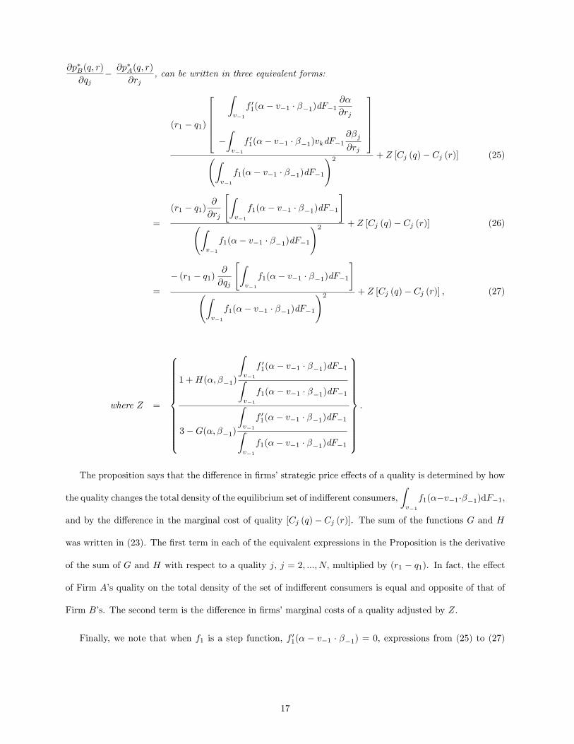
@p�B(q; r)

@qj� @p�A(q; r)

@rj, can be written in three equivalent forms:

(r1 � q1)

266664Zv�1

f 01(�� v�1 � ��1)dF�1@�

@rj

�Zv�1

f 01(�� v�1 � ��1)vkdF�1@�j@rj

377775 Z

v�1

f1(�� v�1 � ��1)dF�1

!2 + Z [Cj (q)� Cj (r)] (25)

=

(r1 � q1)@

@rj

"Zv�1

f1(�� v�1 � ��1)dF�1

# Z

v�1

f1(�� v�1 � ��1)dF�1

!2 + Z [Cj (q)� Cj (r)] (26)

=

� (r1 � q1)@

@qj

"Zv�1

f1(�� v�1 � ��1)dF�1

# Z

v�1

f1(�� v�1 � ��1)dF�1

!2 + Z [Cj (q)� Cj (r)] ; (27)

where Z =

8>>>>>>>>>>><>>>>>>>>>>>:

1 +H(�; ��1)

Zv�1

f 01(�� v�1 � ��1)dF�1Zv�1

f1(�� v�1 � ��1)dF�1

3�G(�; ��1)

Zv�1

f 01(�� v�1 � ��1)dF�1Zv�1

f1(�� v�1 � ��1)dF�1

9>>>>>>>>>>>=>>>>>>>>>>>;:

The proposition says that the di¤erence in �rms�strategic price e¤ects of a quality is determined by how

the quality changes the total density of the equilibrium set of indi¤erent consumers,Zv�1

f1(��v�1���1)dF�1,

and by the di¤erence in the marginal cost of quality [Cj (q)� Cj (r)]. The sum of the functions G and H

was written in (23). The �rst term in each of the equivalent expressions in the Proposition is the derivative

of the sum of G and H with respect to a quality j, j = 2; :::; N; multiplied by (r1 � q1). In fact, the e¤ect

of Firm A�s quality on the total density of the set of indi¤erent consumers is equal and opposite of that of

Firm B�s. The second term is the di¤erence in �rms�marginal costs of a quality adjusted by Z.

Finally, we note that when f1 is a step function, f 01(� � v�1 � ��1) = 0, expressions from (25) to (27)

17

simplify to only the term related to the di¤erence in marginal costs:

@p�B(q; r)

@qj� @p

�A(q; r)

@rj=1

3[Cj (q)� Cj (r)] :

In other words, when the di¤erentiated dimension has a uniform-distribution valuation, each �rm�s quality

raises the markup by the same amount, so the strategic price reaction e¤ects are all in the marginal-cost

di¤erence.

3.3 Equilibrium qualities

Given the equilibrium prices p�A(q; r) and p�B(q; r) in Stage 2, we write the pro�t functions in Stage 1 in

terms of qualities:

�A(p�A(q; r); p

�B(q; r); q; r) =

Zv�1

F1(ev1(v�1; p�; q; r))dF�1 [p�A(q; r)� C(q)] (28)

�B(p�A(q; r); p

�B(q; r); q; r) =

Zv�1

[1� F1(ev1(v�1; p�; q; r))]dF�1 [p�B(q; r)� C(r)] ; (29)

where ev1(v�1; p�; q; r) � p�B(q; r)� p�A(q; r)r1 � q1

�PN

k=2 vkrk � qkr1 � q1

. For subgame-perfect equilibrium prices, p�,

equilibrium qualities are q� and r� that are mutual best responses:

q� � (q�1 ; :::; q�N ) = argmax

q

Zv�1

F1(ev1(v�1; p�(q; r�); q; r�))dF�1 [p�A(q; r�)� C(q)]

r� � (r�1 ; :::; r�N ) = argmax

r

Zv�1

[1� F1(ev1(v�1; p�(q�; r); q�; r))]dF�1 [p�B(q�; r)� C(r)] ;where p�(q; r) � (p�A(q; r); p�B(q; r)).

Qualities qi, i = 1; :::; N a¤ect Firm A�s pro�t (28) in three ways. First, they have a direct e¤ect through

the costs, C(q), as well as the demand. Second, they a¤ect the pro�t through Firm A�s own equilibrium price

p�A(q; r). Third, they a¤ect the pro�t through Firm B�s equilibrium price p�B(q; r), captured by @p�B=@qi.

Because the equilibrium prices p�A(q; r) and p�B(q; r) are mutual best responses in the price subgame in Stage

2, the envelope theorem applies. That is, Firm A�s qualities qi, i = 1; :::; N have second-order e¤ects on its

own pro�t (28) through its equilibrium price; the second e¤ect can be ignored.

18

The �rst-order derivative of (28) with respect to qi is

�"Z

v�1

F1(ev1(v�1; p�(q; r�); q; r�))dF�1#Ci(q)+@

@qi

Zv�1

F1(ev1(v�1; p�(q; r�); q; r�))dF�1 [p�A(q; r�)� C(q)]| {z }e¤ects of quality qi on cost and demand

(30)

+@

@p�B

(Zv�1

F1(ev1(v�1; p�(q; r�); q; r�))dF�1) @p�B@qi

[p�A(q; r�)� C(q)]| {z }

e¤ect of quality on Firm B�s price

; i = 1; :::; N; (31)

where the (partial) derivative of pro�t with respect to pA has been ignored. The terms in (30) describe how

a quality a¤ects cost and demand, whereas the term in (31) describes the strategic e¤ect of a quality on the

rival�s price.

Next, we use the same steps to obtain the �rst-order derivatives of Firm B�s pro�t (29) with respect to

ri, and these are

�"Z

v�1

[1� F1(ev1(v�1; p�(q�; r); q�; r))]dF�1#Ci(r)+@

@ri

(Zv�1

[1� F1(ev1(v�1; p�(q�; r); q�; r))]dF�1) [p�B(q�; r)� C(r)]| {z }e¤ects of quality on cost and demand

(32)

+@

@p�A

(Zv�1

[1� F1(ev1(v�1; p�(q�; r); q�; r))]dF�1) @p�A@ri

[p�A(q; r�)� C(r)]| {z }

e¤ect of quality ri on Firm A�s price

; i = 1; :::; N: (33)

These expressions carry the same interpretations as those in the �rst-order derivatives for Firm A.

We now state the main result on equilibrium qualities. We obtain the set of equations in the next

proposition by �rst simplifying the �rst-order derivatives and then setting them to zero. For simpli�cation,

we use the basic demand function (3) and equilibrium prices (12) and (13) in Proposition 1, and �nally drop

common factors in the �rst-order derivatives. (Details are in the proof.)

Proposition 3 For the quality-price, multistage game in Subsection 2.2, equilibrium qualities (q�; r�) (under

19

the convention that q�1 < r�1) must satisfy the following 2N equations:

@p�B@q1

+

Zv�1

f1(�� v�1 � ��1)ev�1dF�1Zv�1

f1(�� v�1 � ��1))dF�1� C1(q�) = 0 (34)

@p�A@r1

+

Zv�1

f1(�� v�1 � ��1)ev�1dF�1Zv�1

f1(�� v�1 � ��1))dF�1� C1(r�) = 0; (35)

and for j = 2; :::; N ,

@p�B@qj

+

Zv�1

f1(�� v�1 � ��1)vjdF�1Zv�1

f1(�� v�1 � ��1))dF�1� Cj(q�) = 0 (36)

@p�A@rj

+

Zv�1

f1(�� v�1 � ��1)vjdF�1Zv�1

f1(�� v�1 � ��1))dF�1� Cj(r�) = 0: (37)

where � and �j are the functions in (10) and (11), respectively, and ev�1 is ev�1(v�1; q�; r�), the solution of theintegral equation in Lemma 1.

The properties of equilibrium qualities in (34) and (36) can be explained as follows. There are two e¤ects.

The �rst term in each expression is the price-reaction e¤ect : it describes how Firm A�s qualities q1 and qj ,

j = 2; :::; N a¤ect the rival�s price in the continuation subgame. In fact, all the price-reaction e¤ects are

written out in equations (16) to (19) above.

The second e¤ect concerns the average valuation of the jth quality among the equilibrium set of indi¤erent

consumers� the integrals in (34) and (36)� and the jth quality�s marginal contribution to the per-unit

cost� Cj �@C(q)

@qj. These two terms together form the Spence e¤ect. Indeed, Spence (1975) shows that a

pro�t-maximizing �rm chooses the e¢ cient quality for the marginal consumer (and then raises the price to

extract the marginal consumer�s surplus).7 The same price-reaction and Spence e¤ects apply to Firm B�s

equilibrium quality choices described by (35) and (37).

7Let P (D; q) be the price a �rm can charge when it sells D units of its good at quality q = (q1; :::; qN ). Let C(D; q)be the cost when the �rm produces D units at quality q. Pro�t is DP (D; q)�C(D; q). The pro�t-maximizing qualityqi is given by D

@P

@qi=@C

@qi. Hence the quality valuation of the marginal consumer

@P

@qiis equal to the marginal

contribution of quality i to per-unit cost@C=@qiD

. See Spence (1975, p419; equation (8)).

20

Because the two �rms face the same equilibrium set of indi¤erent consumers, the Spence e¤ect pushes

them to choose the same qualities. The price-reaction e¤ects generally put the �rms in a race situation.

Prices are strategic complements, so each �rm wants to use its qualities to raise the rival�s price. The

price-reaction e¤ect dictates how much a �rm�s equilibrium quality deviates from the e¢ cient quality for the

equilibrium set of indi¤erent consumers. The �rm that has a stronger strategic price-reaction e¤ect deviates

more.

If the two �rms were playing another game in which prices and qualities were chosen concurrently (one

with merged Stages 1 and 2 in the extensive form in Subsection 2.2), the price-reaction e¤ect would vanish.

Then the Spence e¤ect would dictate equilibrium strategies. Each �rm would choose the qualities optimal

for the average valuations of the common set of marginal consumers, so �rms choose the same level for each

quality attribute. Firms must then set their prices at marginal cost. (For an illustration of a game with

�rms choosing prices and qualities concurrently, see Ma and Burgess (1993)).

Proposition 3 holds the key to the understanding of equilibrium product di¤erentiation with multiple

qualities, to which we now turn.

3.4 Quality di¤erentiation

Proposition 3 draws a connection between the price-reaction e¤ects and qualities�marginal contributions to

unit production cost. We state this formally:

Corollary 1 At the equilibrium (q�; r�), a �rm�s jth quality contributes more to its own unit production cost

than a rival�s jth quality contributes to the rival�s unit production cost if and only if the �rm�s price-reaction

e¤ect of that quality is stronger than the rival�s. That is, for each j = 2; :::; N , the following are equivalent:

i) Cj(q�) < Cj(r�),

ii)@p�B(q

�; r�)

@qj<@p�A(q

�; r�)

@rj,

iii) the three equivalent expressions (25), (26), and (27) in Proposition 2 are negative at equilibrium (q�; r�).

Corollary 1 follows from Proposition 3 straightfowardly; we simply take the di¤erence between �rst-order

conditions. On the cost side, the fundamental issue is how much a quality contributes to the unit production

21

cost. On the strategic side, the fundamental issue is how much a quality a¤ects the rival�s price. The quality

race concerns only these two issues. However, the corollary does not directly address the equilibrium quality

levels. We have used a general cost function, so it is quite possible that Cj(q�) < Cj(r�) but q�j > r�j . (For

an illustration, see the example after Corollary 3.) Sharper results can be obtained from the following (with

proof omitted):

Corollary 2 Suppose that the cost function C is separable:

C(q) = C(q1; q2; :::; qN ) = 1(q1) + 2(q2); ::: N (qN );

where i is an increasing and convex function, so Ci(q) = 0i(qi), i = 1; 2; :::; N . In an equilibrium (q�; r�),

for j = 2; :::; N ,

q�j < r�j ()

@p�B(q�; r�)

@qj<@p�A(q

�; r�)

@rj:

With separable cost, a quality�s contribution to the unit production cost is independent of other qualities.

A �rm having a stronger price-reaction e¤ect at a quality than its rival�s must choose a higher quality than

its rival�s quality. In the literature, the separable cost function has been adopted. Corollaries 1 and 2 can be

read as a caution. The fundamental issue is how a quality contributes to the production cost. For a model

with many qualities, a quality�s contribution to production cost depends on the entire vector of qualities.

Corollaries 1 and 2 together say that such interdependence is important; see also the example following the

next result.

Next, we consider speci�c quality valuation density functions commonly used in the literature. Recall

that, with a step function the di¤erence of the price e¤ects reduces to 13 [Cj(q)� Cj(r)] : Hence:

Corollary 3 Suppose that f1 is a step function, so f 01 = 0 almost everywhere. In an equilibrium (q�; r�),

Cj(q�) = Cj(r

�) and@p�B(q

�; r�)

@qj=@p�A(q

�; r�)

@rj, j = 2; :::; N . Furthermore, if C is separable, then q�j = r

�j ,

j = 2; :::; N ; in other words, qualities 2 through N are nondi¤erentiated.

Corollary 3 presents a striking result. First, the uniform distribution is the most common quality-

valuation assumption in the product-di¤erentiation literature, and it is a step function. Under the uniform-

22

distribution assumption, �rms must have identical price-reaction e¤ects.8 Next, if the cost function is

separable, another common assumption in the literature, then all equilibria will have di¤erentiation in

exactly one quality!

Identical price-reaction e¤ects and separable cost are responsible for quality nondi¤erentiation. Here is a

simple example to show that even when there is no di¤erence between price-reaction e¤ects between �rms,

equilibrium product di¤erentiation arises entirely because of cost consideration. Let the cost function (for

a model with two qualities) be C(q1; q2) = 12q21 + �q1q2 +

12q22 , for some parameter �. Then C1(q1; q2) =

q1 + �q2, and C2(q1; q2) = �q1 + q2. Suppose that f1 is a step function, so �rms�price-reaction e¤ects are:

@p�B@qj

� @p�A

@rj= 1

3 [C2(q1; q2)� C2(r1; r2)]. According to Corollary 3, C2(q�1 ; q

�2) = C2(r

�1 ; r

�2). In other words,

�q�1 + q�2 = �r�1 + r

�2 , and �(r

�1 � q�1) = q�2 � r�2 . By assumption we have q�1 < r�1 in the equilibrium. We

conclude that q�2 > r�2 if and only if � > 0. When qualities have positive spillover on cost (� > 0), then

Firm A�s product has one superior quality and one inferior quality compared to Firm B�s. By contrast,

when qualities have negative spillover (� < 0), Firm A�s qualities are always lower than Firm B�s. (The

equilibrium demand can be likened to the one in Figure 1.)

Corollary 3 has used the convention that in the equilibrium, q�1 < r�1 . The following explains the scope

of the convention.

Corollary 4 Consider the game de�ned by valuation densities fi, i = 1; :::; N , and the separable cost function

C =

NXi=1

i. Suppose that at least one of the densities is a step function.

i) In every subgame-perfect equilibrium, each �rm must choose an identical level in at least one quality.

ii) If in an equilibrium (q�; r�) there is di¤erentiation in the jth quality, so that q�j 6= r�j , and fj is a step

function, j = 1; :::; N , then there is no di¤erentiation in any other quality, so q�k = r�k, for k = 1; 2; :::; N ,

and k 6= j.

In this corollary, we have gotten rid of the convention that in equilibrium Firm A chooses a lower �rst

quality than Firm B. Consider all equilibria of the multistage game, given valuation densities and the

cost function. The e¤ect of any uniform quality-valuation distribution and the separable cost function is

8 In fact, for any subgame (q; r), the di¤erence of the price-reaction e¤ects vanishes when f1 is a step function.

23

quite striking. Suppose that the jth quality has a uniform valuation distribution. If it so happens that in

equilibrium �rms choose q�j 6= r�j , then Corollary 3 applies to the jth quality, so all equilibrium qualities

except the jth must be identical. The only case in which equilibrium di¤erentiation happens in more than

one quality is when q�j = r�j . Then Corollary 3 does not apply to the j

th quality. But this means that there

is (at least) one nondi¤erentiated quality.

Corollary 4 clari�es the �Max-Min-Min...-Min�results in Irmen and Thisse (1998). They consider an N -

dimensional Hotelling model (which can be translated into our N -dimensional quality model). Consumers�

locations are uniformly distributed on the N -dimensional unit hypercube. Consumers�mismatch disutility

is the (weighted) N -dimensional Euclidean distance. Irmen and Thisse derive a subgame-perfect equilibrium

in which the two �rms choose the maximum distance between themselves in one dimension but zero distance

in all other dimensions (p90, Proposition 2). Although Corollary 4 does not address existence of equilibria,

it is consistent with the Irmen-Thisse result. To see this, we can rewrite Corollary 4 as follows: if M of the

qualities have uniformly distributed valuations, 1 � M � N , then at least minfM;N � 1g qualities will be

nondi¤erentiated. This is a slightly more general result than in Irmen and Thisse (1998).

In the vertical di¤erentiation literature, Max-Min results have also �gured prominently. Vandenbosch

and Weinberg (1995) and Lauga and Ofek (2011) are two related papers that use a linear cost function, and

restrict each of two qualities to be in its own bounded interval. In the notation here, in both papers, N = 2,

valuation density fi is uniform, quality qi is to be chosen from interval [qi; qi], i = 1; 2, and unit production

cost at quality q is C(q) = c1q1 + c2q2, for constants c1 and c2. (In fact, the values of c1 and c2 are set at 0

in some parts of the analysis.) The linear cost function does not satisfy our assumption of strict convexity.

Equilibrium qualities generically are corner solutions of �rms�pro�t maximization. In other words, when

the corner solution hits one quality lower bound by one �rm (qi), but an upper bound by the other (qi),

there is maximum quality di¤erentiation. If �rms�corner solutions are at the lower bound or upper bound,

then there is minimum di¤erentiation.

We can interpret Max-Min results in terms of price-reaction and Spence e¤ects. First, according to

Corollary 3, because quality valuations are uniformly distributed, price-reaction e¤ects are the same for both

24

�rms. In the race to use quality to raise the rival�s price, there is no winner. Second, because the cost is linear,

a quality�s marginal contribution to unit production cost Ci(q) is constant. The Spence e¤ect generically

cannot specify an interior solution for the e¢ cient quality for the equilibrium set of indi¤erent consumers.

The Max-Min (or Max-Max) results are driven by the combination of linear costs and uniform valuation

distributions. For a model with strictly convex cost and general valuation distributions, in equilibrium each

�rm generically will choose a di¤erent level for each quality.

4 Examples

In this section, we present three sets of examples of a model with two quality dimensions (N = 2). The

�rst set uses a Cobb-Douglas cost function, and various quality-valuation distributions. These examples

illustrate how characterization of equilibrium prices. The second set uses a quadratic cost function and

uniform-distribution valuations. We solve for the equilibrium conditions explicitly. In the third example we

collapse one valuation distribution, so it becomes e¤ectively a single dimension of quality valuations. This

allows us to connect our results to earlier ones.

4.1 Cobb-Douglas cost, and exponential, trapezoidal, and beta quality-valuationdistributions

Recall that the equilibrium set of indi¤erent consumers is given by ev�1(v�1; q; r) = �(q; r)�PNk=2 vk�k(q; r), vk 2

[vk; vk]; k = 2; :::; N , where �(q; r) is in (10) and �k(q; r) is in (11). For the examples, we consider two qual-

ities, so set N = 2. We also let the valuations v1 and v2 be drawn from the unit interval [0; 1]. We use a

Cobb-Douglas type cost function C(q) = q 1 q�2; with ; � > 1.

Lemma 1 says we can solve for � (q; r) implicitly. In fact, for particular valuation distributions, we can

obtain explicit solutions. This can be achieved by a program such as Mathematica, and that is what we have

done. Mathematica codes are available from the authors.

The �rst example is the truncated exponential distribution. We set the valuation densities to fi(vi) =

exp

��viki

�hki

�1� exp

�� 1ki

��i�1, i 2 f1; 2g, where ki > 0 is the parameter for the distribution. Applying

25

Lemma 1, and after integration, we obtain the implicit function that de�nes �(q; r):

� =q 1 q

�2 � r

1 r�2

q1 � r1�

�exp

�1

k1

�+ 1

��exp

�1

k2

�� 1�exp

��� 1k1

��k1 +

k2(r2 � q2)q1 � r1

�exp

�1

k2

�� exp

�q2 � r2

k1 (q1 � r1)

� + 2k1:

Getting an explicit solution for � is infeasible, but it is unnecessary to do so.

The second example is a trapezoidal distribution. Here, we set fi(vi) = 1 � ki + 2kivi; i 2 f1; 2g, with

ki 2 [�1; 1]. The uniform distribution is a special case with ki = 0. Applying Lemma 1, we obtain the

implicit function that de�nes �:

� =q 1 q

�2 � r

1 r�2

q1 � r1+

6�[(�� 1)k2 + 1]�(k2 + 3)[(2�� 1)k2 + 1](q2 � r2)

q1 � r1+k2(k2 + 2)(q2 � r2)2

(q1 � r1)2� 3

k2

��6�+ (k2 + 3)(q2 � r2)

q1 � r1+ 3

�� 3

:

This is a quadratic equation in �, so an explicit solution for � is readily available (although the explicit

solution consists of complicated functions of qualities).

For the special case of the uniform distribution, we have

� =q 1 q

�2 � r

1 r�2

q1 � r1� 2�+ q2 � r2

q1 � r1+ 1

or

� =1

3

�q 1 q

�2 � r

1 r�2

q1 � r1+q2 � r2q1 � r1

+ 1

�: (38)

Clearly, the uniform distribution makes computation easy, but it forces the �rms�price-reaction e¤ects to

be identical.

Our last example is the beta distribution. We set fi(vi) =v(ai�1)i (1�vi)(bi�1)Z 1

0

x(ai�1)i (1�xi)(bi�1)dx

; i 2 f1; 2g, with

ai; bi > 0: As an illustration, we let a1 = a2 = 2 and b1 = b2 = 5, then Lemma 1 yields the following implicit

function for �:

� =q 1 q

�2 � r

1 r�2

q1 � r1

+1

30

8<: �4620�6 + 792�5(25� + 7)� 2475�4�(15� + 8) + 1100�3�2(35� + 27)�23100�2�3(� + 1) + 840��4(9� + 11)� 42[(25� + 36)�5 + 11]

9=;8<: 462�5 � 66�4(25� + 7) + 165�3�(15� + 8)�55�2�2(35� + 27) + 770��3(� + 1)� 14�4(9� + 11)

9=;;

26

which is a sixth-order polynomial in �.

In all the previous examples, we must have equilibrium quality di¤erentiation in both dimensions because

the distributions of the quality valuations are non-uniform and because the cost function is nonseparable.

We also obtain di¤erentiation in both dimensions when valuations are uniformly distributed and when the

solution for � is in (38) because the cost function is nonseparable.

4.2 Quadratic cost function and uniform distributions

We consider again N = 2. Now the valuations v1 and v2 are uniformly distributed on the interval [1; 2]. We

use the quadratic cost function

C(q1; q2) =1

2q21 + �q1q2 +

1

2q22

which exhibits a positive cost spillover if and only if � > 0, and which is separable if � = 0. (This quadratic

cost function was brie�y mentioned in the discussion following Corollary 3.)

Solving for � (q; r) the integral equation in Lemma 1 we obtain a unique solution:

� (q; r) =1

6

q21 + q2 (6 + q2)� r2 (6 + r2) + 2q1 (1 + �q2)� r1 (6 + r1 + 2�r2)q1 � r1

(39)

The equilibrium set of marginal consumers is

ev�1(v2; q; r) = 1

6

q21 + q2 (6 + q2)� r2 (6 + r2) + 2q1 (1 + �q2)� r1 (6 + r1 + 2�r2)q1 � r1

� q2 � r2q1 � r1

v2:

The expressions for G (�; �2) and H (�; �2) are

G (�; �2) =1

6

q21 + q2 (q2 � 3)� r2 (r2 � 3) + 2�q1q2 � r1 (r1 + 2�r2)q1 � r1

H (�; �2) = 1� 16

q21 + q2 (q2 � 3)� r2 (r2 � 3) + 2�q1q2 � r1 (r1 + 2�r2)q1 � r1

:

Price e¤ects are:

@p�A@r1

= G+ (r1 � q1)@G

@r1=1

3(r1 + �r2)

@p�B@q1

= �H + (r1 � q1)@H

@q1=1

3(�3 + q1 + �q2)

@p�A@r2

= (r1 � q1)@G

@r2=1

6(�3 + 2r2 + 2�r1) (40)

@p�B@q2

= (r1 � q1)@H

@q2=1

6(�3 + 2q2 + 2�q1) (41)

27

These price e¤ects are simple. A �rm�s in�uence on the rival�s price is independent of the rival�s qualities, a

consequence of the uniform-distribution assumption.

Moreover,@p�A@r1

>@p�B@q1

for all values of �. We con�rm that in any equilibrium r1 > q1. However,@p�A@r2

can be smaller or larger than@p�B@q2

. In fact, we also con�rm Proposition 2:

@p�B (q; r)

@q2� @p

�A (q; r)

@r2=1

3[C2(q1; q2)� C2(r1; r2)] =

1

3[q2 � r2 + � (q1 � r1)]

Solving the system of equations of the �rst-order conditions in Proposition 3 we �nd:

q�1 =

�3

4

�1� 2�1� �2

; q�2 =

�3

4

�2� �1� �2

; r�1 =

�3

4

�3� 2�1� �2

; r�2 =

�3

4

�2� 3�1� �2

: (42)

Any equilibrium qualities must be those in (42).

Moreover, substituting the previous qualities into the expressions for the price e¤ects@p�A (q; r)

@r2and

@p�B (q; r)

@q2, in (40) and in (41), respectively, we verify that the price e¤ects of the second qualities are the

same at an equilibrium.

Finally, for some speci�c values of the parameter �, we have

(1) If � = 0; q�1 = 3=4; q�2 = 3=2; r�1 = 9=4; r�2 = 3=2:(2) If � = 1=2; q�1 = 0; q�2 = 3=2; r�1 = 2; r�2 = 1=2:(3) If � = �1=2; q�1 = 2; q�2 = 5=2; r�1 = 4; r�2 = 7=2:

(43)

Case (1) in (43) illustrates Corollary 3: with a separable cost function and uniform distributions only

the �rst dimension of quality is di¤erentiated. Moreover, in equilibrium, the two �rms must choose q�2 =

r�2 = E [v2]. In Case (2), for positive cost spillover, Firm A produces a superior second quality than Firm B.

Conversely, in Case (3), for negative cost spillover, Firm A produces an inferior second quality than Firm B.

4.3 Collapsing one valuation distribution in a model with two qualities

We have assumed that there are at least two qualities. However, we can easily modify the model to relate

directly to Anderson, Goeree and Ramer (1997) who consider a single-dimension horizontal model with a

general consumer-location distribution, and to Garella and Lambertini (2014), who consider a two-dimension

vertical model with consumers having homogenous valuations on one quality. The modi�cations are setting

N = 2, and collapsing the valuation distribution of the second quality into a single point, say bv2 > 0.

28

For given qualities (q1; q2) = q from Firm A and qualities (r1; r2) = r from Firm B, if consumers value

the second quality at bv2, the set of indi¤erent consumers in (3) becomes a single point. The equilibriumprices in (6) and (7) simplify to

p�A � C(q) =F1(ev1)f1(ev1) (r1 � q1) � G1(ev1)(r1 � q1) (44)

p�B � C(r) =1� F1(ev1)f1(ev1) (r1 � q1) � H1(ev1)(r1 � q1); (45)

where

ev1(bv2; p�; q; r) = p�B � p�Ar1 � q1

� bv2 r2 � q2r1 � q1

: (46)

Here, we have added the subscript 1 on the price-cost margins G and H to distinguish them from the general

ones above.9 The logconcavity of f1 implies that G1 is strictly increasing, and that H1 is strictly increasing

(Anderson, Goeree and Ramer 1997, p106). Equations (44) and (45), together with the indi¤erent consumer

(46), de�ne a price equilibrium. Let ev�1(bv2; q; r) = ev1(bv2; p�; q; r), where p� is the vector of equilibrium prices

which are functions of q and r. These three equations correspond to equations (2.1), (2.2) and (2.3) in

Anderson, Goeree and Ramer (1997, p107).

We use (44) and (45) to substitute for equilibrium prices in (46). After some simpli�cation we obtain the

implicit de�nition of ev�1 :ev�1 +G1(ev�1)�H1(ev�1) = [bv2q2 � C(q)]� [bv2r2 � C(r)]

r1 � q1: (47)

From (47) we compute the derivatives of ev�1 with respect to the qualities; these correspond to the derivativesof �(q; r) in the proof of Lemma 3. Then we use those derivatives to simplify the price-reaction e¤ects

obtained from the explicit di¤erentiation of (44) and (45) with respect to prices. The various steps are

spelled out in the �rst two parts of Appendix B.

9The functions G1 and H1 are commonly called the reverse hazard rate and hazard rate, respectively.

29

The �rst-order conditions from (34) to (37) in Proposition 3 can be simpli�ed to:

@p�B@q1

+ ev�1 = C1(q�) (48)

@p�B@q2

+ bv2 = C2(q�) (49)

@p�A@r1

+ ev�1 = C1(r�) (50)

@p�A@r2

+ bv2 = C2(r�): (51)

In the third part of Appendix B, we prove that if the cost function C(q) is separable, C(q) = 1(q1)+ 2(q2),

then bv2 = 02(q�2) = 02(r

�2), so q

�2 = r�2 . This is a natural result: �rms cannot di¤erentiate a quality when

consumers have homogenous valuations on that quality when quality costs are separable.

Finally, after putting the price-reaction e¤ects into (48) and (50) (see the last part of Appendix B for

the computation of the price-reaction e¤ects), we show that equilibrium qualities q�1 and r�1 must satisfy:

ev�1 = C1(q�) +H1(ev�1)� H 0

1(ev�1)1 +G01(ev�1)�H 0

1(ev�1)�C(r�)� C(q�)

r�1 � q�1� C1(q�)

�(52)

ev�1 = C1(r�)�G1(ev�1)� G01(ev�1)

1 +G01(ev�1)�H 01(ev�1)

�C1(r

�)� C(r�)� C(q�)r�1 � q�1

�; (53)

where

ev�1 �H1(ev�1) +G1(ev�1) = [bv2q�2 � C(q�)]� [bv2r�2 � C(r�)]r�1 � q�1

: (54)

When the cost function is separable, we have q�2 = r�2 , so (54) becomes

ev�1 +G1(ev�1)�H1(ev�1) = 1(r�1)� 1(q�1)r�1 � q�1

:

Furthermore, equations (52) and (53) become

ev�1 = 01(q�1) +H1(ev�1)� H 0

1(ev�1)1 +G01(ev�1)�H 0

1(ev�1)� 1(r

�1)� 1(q�1)r�1 � q�1

� 01(q�1)�

ev�1 = 01(r�1)�G1(ev�1)� G01(ev�1)

1 +G01(ev�1)�H 01(ev�1)

� 01(r

�1)�

1(r�1)� 1(q�1)r�1 � q�1

�:

These last three equations together with the equilibrium prices correspond to equations (2.8) and (2.10) on

pages 108 and 109 of Anderson, Goeree, and Ramer (1997).

30

Garella and Lambertini (2014) use a discontinuous cost function: a �rm producing z units of the good

at quality (q1; q2) has a total cost of cz + T (q1; q2) if q1 > q1 , but only T (q1; q2) if q1 = q1, where q1 > 0

and c > 0 are �xed parameters, and T is increasing when q1 > q1. Consumers have homogenous preferences

on the second quality, but their valuations on the �rst quality follow a uniform distribution. They derive

equilibria in which �rms choose di¤erent levels in both qualities. We use a continuous cost function, but if

costs are nonseparable, equilibria in our model will also exhibit di¤erentiations in both qualities. Because

of the uniform distribution,@p�B (q

�; r�)

@q2=@p�A (q

�; r�)

@r2, and C2(q�) = C2(r�), which generally implies that

q�2 6= r�2 . The example presented just before Corollary 3 and the simulations in Subsection 4.2 can be used

again for this illustration.

5 Conclusion

We reexamine the principle of product di¤erentiation relaxing price competition in the classical quality-price

game. The environment for analysis in our model is more general than existing works. Yet, we are able to

characterize equilibria without compromise, thereby con�rming the principle of di¤erentiation. The outcome

of minimum di¤erentiation in earlier works can be attributed to consumers�quality valuations (or location)

being uniformly distributed and quality cost (or mismatch disutility) being separable. The principle of

product di¤erentiation is robust: �rms tend to choose di¤erent quality attributes.

Various open questions remain. First, unlike previous works that use explicit functional forms, we have

used a general setup. Whereas direct computation of equilibria has been the main technique, we have used

only necessary conditions of equilibria. Although we do not provide existence results, our characterization

applies to each equilibrium when it does exist. The existence and uniqueness issues are beyond the scope

of the current research, but it may turn out to be a rewarding endeavor. Second, our innovation is the

representation of the price equilibrium by the solution of an integral equation. This technique is uncommon.

In fact, economists seldom have to solve integral equations. It may well be that our technique can shed

light on other models with multiple preferences or cost attributes. Third, we assume linear preferences:

each quality bene�ts a consumer at a constant rate. The linearity assumption is so ubiquitous in modern

microeconomics that relaxing this is both challenging and consequential. Finally, it seems that extending

31

our environment to allow for consumers having correlated valuations between qualities may be worthwhile.

Our framework may just be rich enough for this extension. One may work with conditional joint densities

to derive demand functions. Of course, the exact formulation will be future research.

32

Appendix A: Proofs of Lemmas, Propositions, and Corollaries

Proof of Lemma 1: Equilibrium prices p�A and p�B depend on qualities (q; r), so the right-hand side of (8)

is (a¢ ne) linear in v2; :::; vN . The solution ev�1(v�1; q; r) of (9) also satis�es (8), so it must also be linear inv2; :::; vN . Therefore, we write ev�1(v�1; q; r) = �(q; r)�PN

k=2 vk�k(q; r), vk 2 [vk; vk]; k = 2; :::; N for some

functions �, and �k, k = 2; :::; N . Then we substitute ev�1(v�1; q; r) by �(q; r)�PNk=2 vk�k(q; r) in (9) to get

�(q; r)�NPk=2

vk�k(q; r) =

Zv�1

h1� 2F1(�(q; r)�

PNk=2 vk�k(q; r))

idF�1Z

v�1

f1(�(q; r)�PN

k=2 vk�k(q; r))dF�1

+C(r)� C(q)r1 � q1

�NPk=2

vkrk � qkr1 � q1

; for vk 2 [vk; vk]; k = 2; :::; N:

Because this is true for every v2; :::; vN , the equations (10) and (11) in the lemma follow.

Proof of Lemma 2: From the de�nitions (14) and (15), at each (q; r), we have:

G(�; ��1) +H(�; ��1) =1Z

v�1

f1(�� v�1 � ��1)dF�1:

Hence

d ln(G+H) + d lnZv�1

f1(�� v�1 � ��1)dF�1 = 0;

so the �rst statement of the lemma follows.

Because (20) holds for each (q; r), we can partially di¤erentiate it with respect to � and �j , j = 2; :::; N ,

to obtain (21) and (22).

Proof of Lemma 3: From (11), the functions �j(q; r) are �j =rj � qjr1 � q1

, j = 2; :::; N . Hence,

@�j@q1

=rj � qj(r1 � q1)2

= �@�j@r1

; and@�j@qj

= � 1

r1 � q1= �

@�j@rj

; j = 2; :::; N; (55)

and all partial derivatives of �j with respect to qk or rk, k 6= j, vanish. These prove the second equality

in (24).

From de�nitions of G and H in (14) and (15), we write (10) as

�+G��; ��1

��H

��; ��1

�=C(r)� C(q)r1 � q1

: (56)

33

We totally di¤erentiate (56) to obtain�1 +

@G

@�� @H@�

�d�+

NXk=2

�@G

@�k� @H

@�k

�d�j = d

�C(r)� C(q)r1 � q1

�; j = 2; :::; N:

Using (55), we obtain the partial derivatives of � with respect to each quality, and then simplify them to:�1 +

@G

@�� @H@�

�@�

@q1= �

�@G

@�1� @H

@�1

�rj � qj(r1 � q1)2

� C1(q)

(r1 � q1)+

�C(r)� C(q)(r1 � q1)2

�

�1 +

@G

@�� @H@�

�@�

@r1=

�@G

@�1� @H

@�1

�rj � qj(r1 � q1)2

+C1(r)

(r1 � q1)��C(r)� C(q)(r1 � q1)2

�(57)�

1 +@G

@�� @H@�

�@�

@qj=

�@G

@�j� @H

@�j

�1

(r1 � q1)� Cj(q)

(r1 � q1)j = 2; :::; N

�1 +

@G

@�� @H@�

�@�

@rj= �

�@G

@�j� @H

@�j

�1

(r1 � q1)+

Cj(r)

(r1 � q1)j = 2; :::; N;

where Ci(q) �@C(q)

@qidenotes the ith partial derivative of the cost function C. The �rst part of (24) follows

by summing up the �rst two equations and the last two equations in (57) to compute@�(q; r)

@qi+@�(q; r)

@ri,

i = 1; :::; N .

Proof of Proposition 2: From (18) and (19), we have

@p�B(q; r)

@qj� @p

�A(q; r)

@rj= (r1 � q1)

��@H

@�

@�

@qj+@H

@�j

@�j@qj

���@G

@�

@�

@rj+@G

@�j

@�j@rj

��; j = 2; :::; N:

Using Lemma 3, we have@�

@qj=

Cj (r)� Cj (q)

(r1 � q1)�1 +

@G

@�� @H@�

� � @�

@rjand

@�j@qj

= �@�j@rj

, and substitute them

into the above to obtain:

@p�B(q; r)

@qj� @p

�A(q; r)

@rj

= (r1 � q1)

8>><>>:2664@H@�

0BB@ Cj (r)� Cj (q)

(r1 � q1)�1 +

@G

@�� @H@�

� � @�

@rj

1CCA� @H

@�j

@�j@rj

3775� �@G@� @�@rj + @G

@�j

@�j@rj

�9>>=>>;= (r1 � q1)

���@H@�

@�

@rj� @H

@�j

@�j@rj

���@G

@�

@�

@rj+@G

@�j

@�j@rj

��+@H

@�

[Cj (r)� Cj (q)]�1 +

@G

@�� @H@�

�= �(r1 � q1)

��@G

@�+@H

@�

�@�

@rj+

�@G

@�j+@H

@�j

�@�j@rj

�+@H

@�

[Cj (r)� Cj (q)]�1 +

@G

@�� @H@�

� :

34

Next, we de�ne

Z � @H

@�

1�1 +

@G

@�� @H@�

� :We use (21) and (22) in Lemma 2 to obtain

@p�B(q; r)

@qj� @p

�A(q; r)

@rj

=

(r1 � q1)Zv�1

f 01(�� v�1 � ��1)dF�1 Zv�1

f1(�� v�1 � ��1)dF�1

!2 @�

@rj�(r1 � q1)

Zv�1

f 01(�� v�1 � ��1)vjdF�1 Zv�1

f1(�� v�1 � ��1)dF�1

!2 @�j@rj

+ Z [Cj (q)� Cj (r)]

=

(r1 � q1) Z

v�1

f 01(�� v�1 � ��1)dF�1@�

@rj�Zv�1

f 01(�� v�1 � ��1)vjdF�1@�j@rj

! Z

v�1

f1(�� v�1 � ��1)dF�1

!2 + Z [Cj (q)� Cj (r)] ; (58)

which gives (25). Then we further write the �rst term in (58) as

(r1 � q1)@

@rj

"Zv�1

f1(�� v�1 � ��1)dF�1

# Z

v�1

f1(�� v�1 � ��1)dF�1

!2 ; (59)

which gives the �rst term in (26). Finally, from Lemma 3, we have@�

@rj=

Cj (r)� Cj (q)

(r1 � q1)�1 +

@G

@�� @H@�

� � @�

@qj

and@�j@rj

= �@�j@qj

, so (59) also equals

�(r1 � q1)

@

@qj

"Zv�1

f1(�� v�1 � ��1)dF�1

# Z

v�1

f1(�� v�1 � ��1)dF�1

!2 ;

which gives the �rst term in (27).

Finally, from the de�nition of G��; ��1

�and H

��; ��1

�in (14) and (15), we have:

@

@�G��; ��1

�= 1�

Zv�1

f 01(�� v�1 � ��1)dF�1Zv�1

F1(�� v�1 � ��1)dF�1 Zv�1

f1(�� v�1 � ��1)dF�1

!2

@

@�H��; ��1

�= �1�

Zv�1

f 01(�� v�1 � ��1)dF�1Zv�1

�1� F1(�� v�1 � ��1)

�dF�1 Z

v�1

f1(�� v�1 � ��1)dF�1

!2 :

35

After we substitute these into the de�nition of Z, we obtain the same expression for Z in the Proposition.

Proof of Proposition 3: We begin by simplifying Firm A�s �rst-order derivatives with respect to

qualities. First, for (30) we use (3) to obtain

@

@qj

Zv�1

F1(ev1(v�1; p�(q; r�); q; r�))dF�1=

1

r1 � q1

Zv�1

f1(ev1(v�1; p�(q; r�); q; r�))vjdF�1 j = 2; :::; N:

Second, for (31), again we use (3) to obtain

@

@p�B

Zv�1

F1(ev1(v�1; p�(q; r�); q; r�))dF�1=

1

r1 � q1

Zv�1

f1(ev1(v�1; p�(q; r�); q; r�))dF�1:We then substitute these expressions into (30) and (31), and the �rst-order derivative of Firm A�s with

respect to quality qj , j = 2; :::; N , becomes

�"Z

v�1

F1(ev1(v�1; p�(q; r�); q; r�))dF�1#Ci(q)+

1

r1 � q1

Zv�1

f1(ev1(v�1; p�(q; r�); q; r�))vjdF�1 [p�A(q; r�)� C(q)] (60)

+1

r1 � q1

Zv�1

f1(ev1(v�1; p�(q; r�); q; r�))dF�1 @p�B@qi

[p�A(q; r�)� C(q)] :

We now evaluate (60) at the equilibrium qualities, so replace ev1(v�1; p�(q�; r�); q�; r�)) as ev�1(v�1; q�; r�) =�(q�; r�)� v�1 � ��1(q�; r�). Using the equilibrium price (12) in Proposition 1

p�A(q�; r�)� C(q�)r�1 � q�1

=

Zv�1

F1(�� v�1 � ��1))dF�1Zv�1

f1(�� v�1 � ��1))dF�1;

we simplify the �rst-order derivative of Firm A�s pro�t with respect to qj to

"Zv�1

F1(�� v�1 � ��1)dF�1

#2664@p�B@qj +Zv�1

f1(�� v�1 � ��1)vjdF�1Zv�1

f1(�� v�1 � ��1))dF�1� Cj(q)

3775 ; j = 2; :::; N;

where we have omitted the arguments in � and ��1. We set this to zero to obtain the �rst-order condition

for q�j :

@p�B@qj

+

Zv�1

f1(�� v�1 � ��1)vjdF�1Zv�1

f1(�� v�1 � ��1))dF�1� Cj(q�) = 0 j = 2; :::; N:

36

For brevity we do not lay out all the steps for obtaining the �rst-order condition of Firm A�s equilibrium

quality q1, but the key di¤erence is that (3) yields@ev1@q1

=ev1

r1 � q1. The e¤ect of quality q1 on demand now

becomes

@

@q1

Zv�1

F1(ev1(v�1; p�(q; r�); q; r�))dF�1=

1

r1 � q1

Zv�1

f1(ev1(v�1; p�(q; r�); q; r�))~v1dF�1:Following the same steps, we obtain the following �rst-order condition for q�1

@p�B@q1

+

Zv�1

f1(�� v�1 � ��1)ev�1dF�1Zv�1

f1(�� v�1 � ��1))dF�1� C1(q�) = 0:

The �rst-order conditions for Firm B�s equilibrium qualities are derived analogously, so we do not repeat

the steps here.

Proof of Corollary 1: For each j = 2; :::; N , the terms with the integrals are the same in the two

equations in (36) and (37). Taking their di¤erence, we have

@p�B@qj

� @p�A

@rj= Cj(q

�)� Cj(r�),

and the equivalence of i) and ii) in the Corollary follows. Then we simply apply Proposition 2 on the

equilibrium (q�; r�) for the equivalence of ii) and iii).

Proof of Corollary 3: We actually prove a more general result for the �rst part. Consider any subgame

de�ned by equilibrium quality vectors (q; r). The di¤erence in the �rms�price-reaction e¤ects is in Proposition

2. Obviously, f 01 = 0 by assumption, so (25) becomes@p�B(q; r)

@qj� @p�A(q; r)

@rj= 1

3 [Cj(q)� Cj(r)]. Under

the step-function assumption, Corollary 1 then says that@p�B(q

�; r�)

@qj� @p

�A(q

�; r�)

@rj= 1

3 [Cj(q�)� Cj(r�)] =

Cj(q�) � Cj(r�): Hence it must be Cj(q�) = Cj(r�), j = 2; :::; N . Which also implies that, in equilibrium,

@p�B(q�; r�)

@qj� @p

�A(q

�; r�)

@rj= 0: Finally, we apply Corollary 2 to obtain the nondi¤erentiation result.

Proof of Corollary 4: Let the valuation density of quality j be uniform. Consider an equilibrium

(q�r�). If q�j = r�j , then the �rst part of the corollary is trivially true. Suppose that q

�j 6= r�j . Without loss

of generality we let q�j < r�j . Now we relabel the indexes so that j = 1. Then Corollary 3 applies, and the

�rms choose identical qualities for all quality attributes k = 2; :::; N .

37

Appendix B: On collapsing one valuation distribution in a modelwith two qualities

Derivatives of ev�1 with respect to qualitiesFrom (47) we obtain the derivatives of ev�1 in (54) with respect to the four qualities:

[1 +G01(ev�1)�H 01(ev�1)] @ev�1@q1 =

[bv2q2 � C(q)]� [bv2r2 � C(r)](r1 � q1)2

� C1(q)

r1 � q1

[1 +G01(ev�1)�H 01(ev�1)] @ev�1@q2 =

bv2 � C2(q)r1 � q1

[1 +G01(ev�1)�H 01(ev�1)] @ev�1@r1 = � [bv2q2 � C(q)]� [bv2r2 � C(r)]

(r1 � q1)2+C1(r)

r1 � q1

[1 +G01(ev�1)�H 01(ev�1)] @ev�1@r2 = �bv2 � C2(r)

r1 � q1:

These are the corresponding derivatives of � (q; r) in the proof of Lemma 3.

Price-reaction e¤ects

Next, from (44) and (45) we obtain the following:

@p�A@r1

= G1(ev�1) + (r1 � q1)G01(ev�1)@ev�1@r1@p�A@r2

= (r1 � q1)G01(ev�1)@ev�1@r2 (61)

@p�B@q1

= �H1(ev�1) + (r1 � q1)H 01(ev�1)@ev�1@q1

@p�B@q2

= (r1 � q1)H 01(ev�1)@ev�1@q2 : (62)

The four price-reaction e¤ects can be obtained after the derivatives of ev�1 with respect to qualities aresubstituted by those above.

Firms choosing the same second quality under separable cost function

We now claim that q�2 = r�2 so the two �rms choose the same level for the second quality when cost is

38

separable. To see this, use the expression@ev�1@r2

for (61) to obtain

@p�A@r2

= ��

G01(ev�1)1 +G01(ev�1)�H 0

1(ev�1)�[bv2 � 02(r�2)];

and use the expression@ev�1@q2

above for (62) to obtain

@p�B@q2

=

�H 01(ev�1)

1 +G01(ev�1)�H 01(ev�1)

�[bv2 � 02(q�2)] :

Then we substitute them into (49) and (51) to obtain�H 01(ev�1)

1 +G01(ev�1)�H 01(ev�1)

�[bv2 � 02(q2)] + bv2 = 02(q

�2)

��

G01(ev�1)1 +G01(ev�1)�H 0

1(ev�1)�[bv2 � 02(r�2)] + bv2 = 02(r

�2)

which simplify to �1 +

H 01(ev�1)

1 +G01(ev�1)�H 01(ev�1)

�[bv2 � 02(q2)] = 0

�1� G01(ev�1)

1 +G01(ev�1)�H 01(ev�1)

�[bv2 � 02(r�2)] = 0;

so we have q�2 = r�2 .

Price-reaction e¤ects for characterizing equilibrium qualities q�1 and r�1

We use@ev�1@q1

to compute

@p�B@q1

= �H1(ev�1) + (r1 � q1)H 01(ev�1)@ev�1@q1

= �H1(ev�1) + H 01(ev�1)

1 +G01(ev�1)�H 01(ev�1)

�C(r�)� C(q�)

r�1 � q�1� C1(q�)

�< 0

which exhibits the classical price reaction. Because q1 < r1, if Firm A raises q1, the di¤erence between the

two qualities drops, and Firm B reacts by reducing its price. Similarly, we use@ev1@r1

to compute

@p�A@r1

= G1(ev�1) + (r�1 � q�1)G01(ev�1)@ev1@r1= G1(ev�1) + G01(ev�1)

1 +G01(ev�1)�H 01(ev�1)

�C1(r

�)� C(r�)� C(q�)r�1 � q�1

�> 0;

which again has the classical price reaction.

39

References

[1] Anderson, S., A. De Palma, and J.-F. Thisse (1992). Discrete choice theory of product di¤erentiation,

MIT press, Cambridge, MA.

[2] Anderson, S., J. Goeree, and R. Ramer (1997). �Location, location, location,� Journal of Economic

Theory 77(1):102-127.

[3] Ansari A., N. Economides, and J. Steckel (1998). �The max-min-min principle of product di¤erentia-

tion,�Journal of Regional Science 38(2):207-230.

[4] Belle�amme, P., and M. Peitz (2010). Industrial Organization: Markets and Strategies, Cambridge

University Press, New York.

[5] Benassi, C., A. Chirco, and C. Colombo (2006) �Vertical di¤erentiation and the distribution of income,�

Bulletin of Economic Research 58(4):345-367.

[6] Cabral, L. (2000). Introduction to industrial organization, MIT press, Cambridge, MA.

[7] Caplin, A., and B. Nalebu¤ (1991). �Aggregation and imperfect competition: On the existence of

equilibrium,�Econometrica 59(1):25-59.

[8] Carlton, D., and J. Perlo¤ (2005). Modern industrial organization 4th Ed, Pearson/Addison Wesley,

Reading, MA.

[9] Champsaur, P., and J.-C. Rochet (1989). �Multiproduct duopolists,�Econometrica 57(3):533-557.

[10] Cremer, H. and J.-F. Thisse (1991). �Location models of horizontal di¤erentiation: a special case of

vertical di¤erentiation,�Journal of Industrial Economics 39(4):383 390.

[11] D�Aspremont, C., J. Gabszewicz, and J.-F. Thisse (1979). �Hotellings stability in competition,�Econo-

metrica 47(5):1145-1150.

[12] Degryse, H. and A. Irmen (2001). �Attribute dependence and the provision of quality,�Regional Science

and Urban Economics 31(5):547�569.

40

[13] Gabszewicz, J., and J.-F. Thisse (1979). �Price competition, quality and income disparities,�Journal

of Economic Theory 20:340�359.

[14] Garella, P.G., and L. Lambertini (2014). �Bidimensional vertical di¤erentiation,�International Journal

of Industrial Organization 32:1-10.

[15] Hotelling, H., (1929). �Stability in competition,�Economic Journal 39:41�57.

[16] Irmen, A., and J.-F.Thisse (1998). �Competition in multi-characteristics space: Hotelling was almost

right,�Journal of Economic Theory 78:76�102.

[17] Lauga, D., and E. Ofek (2011). �Product positioning in a two-dimensional vertical di¤erentiation model:

the role of quality costs,�Marketing Science 30(5):903-923.

[18] Loertscher, S., and G. Muehlheusser (2011). �Sequential location games,�RAND Journal of Economics

42(4):639-663.

[19] Ma, C., and J. Burgess (1993). �Quality competition, welfare, and regulation,�Journal of Economics

58(2):153-173

[20] Neven, D. (1986), �On Hotelling�s competition with non-uniform consumer distributions,�Economics

Letters 21:121-126.

[21] Pepall, L., D. Richards, and G. Norman (2014). Industrial organization: contemporary theory and

empirical applications 5th Ed, Wiley, Malden, MA.

[22] Shaked, A., and J. Sutton (1982). �Relaxing price competition through product di¤erentiation,�Review

of Economic Studies 49(1):3�13.

[23] Shaked, A., and J. Sutton (1983). �Natural oligopolies,�Econometrica 51(5):1469�1483.

[24] Spence A.M. (1975) �Monopoly, quality and regulation,�Bell Journal of Economics 6(2):417-429.

[25] Tabuchi, T. (1994). �Two-stage two dimensional spatial competition between two �rms,�Regional Sci-

ence and Urban Economics 24:207-227.

41

[26] Tabuchi, T., and J.-F. Thisse (1995). "Asymmetric equilibria in spatial competition," International

Journal of Industrial Organization 13:213-227.

[27] Tirole, J. (1988). The theory of industrial organization, MIT press, Cambridge, MA.

[28] Vandenbosch, M., and C. Weinberg (1995). �Product and price competition in a two dimensional vertical

di¤erentiation model,�Marketing Science 14(2):224�249.

[29] Vendorp, E.C.H., and A. Majeed (1995). �Di¤erentiation in a two dimensional market,�Regional Science

and Urban Economics 25:75�83.

[30] Yurko, A. (2010). �How does income inequality a¤ect market outcomes in vertically di¤erentiated mar-

kets?�International Journal of Industrial Organization 29:493�503.

42