BNL-93771-2010

KAERI/TR-4068/2010

Joint Development of

Seismic Capability Evaluation Technology

for Degraded Structures and Components

Annual Report for Year 3 Task

Fragility Analysis Methodology for Degraded

Structures and Passive Components

in Nuclear Power Plants

- Illustrated using a Condensate Storage Tank

한국원자력연구원

기술보고서

BNL-93771-2010

KAERI/TR-4068/2010

Joint Development of

Seismic Capability Evaluation Technology

for Degraded Structures and Components

Annual Report for Year 3 Task

Fragility Analysis Methodology for Degraded

Structures and Passive Components

in Nuclear Power Plants

- Illustrated using a Condensate Storage Tank

June 2010

Jinsuo Nie, Joseph Braverman, and Charles Hofmayer

Brookhaven National Laboratory

Upton, NY 11973, USA

Young-Sun Choun, Min Kyu Kim, and In-Kil Choi

Korea Atomic Energy Research Institute

Daejeon, 305-353, Korea

ii

NOTICE/DISCLAIMER

This manuscript has been authored by employees of Brookhaven Science Associates, LLC under Contract No. DE-

AC02-98CH10886 with the U.S. Department of Energy. The United States Government retains a non-exclusive, paid-

up, irrevocable, world-wide license to publish or reproduce the published form of this manuscript, or allow others to do

so, for United States Government purposes.

Neither the United States Government nor any agency thereof, nor any of their employees, nor any of their contractors,

subcontractors, or their employees, makes any warranty, express or implied, or assumes any legal liability or

responsibility for the accuracy, completeness, or any third party’s use or the results of such use of any information,

apparatus, product, or process disclosed, or represents that its use would not infringe privately owned rights. Reference

herein to any specific commercial product, process, or service by trade name, trademark, manufacturer, or otherwise,

does not necessarily constitute or imply its endorsement, recommendation, or favoring by the United States

Government or any agency thereof or its contractors or subcontractors. The views and opinions of authors expressed

herein do not necessarily state or reflect those of the United States Government or any agency thereof.

iii

제 출 문

한국원자력연구원장 귀하

본 보고서를 2010 년도 “열화성능기반 지진리스크 평가시스템 개발” 연구과제의

기술보고서로 제출합니다.

2010. 6

주저자: Jinsuo Nie

공저자: Joseph Braverman

Charles Hofmayer

Young-Sun Choun

Min Kyu Kim

In-Kil Choi

v

ABSTRACT

The Korea Atomic Energy Research Institute (KAERI) is conducting a five-year research project

to develop a realistic seismic risk evaluation system which includes the consideration of aging of

structures and components in nuclear power plants (NPPs). The KAERI research project includes

three specific areas that are essential to seismic probabilistic risk assessment (PRA): (1)

probabilistic seismic hazard analysis, (2) seismic fragility analysis including the effects of aging,

and (3) a plant seismic risk analysis. Since 2007, Brookhaven National Laboratory (BNL) has

entered into a collaboration agreement with KAERI to support its development of seismic

capability evaluation technology for degraded structures and components. The collaborative

research effort is intended to continue over a five year period. The goal of this collaboration

endeavor is to assist KAERI to develop seismic fragility analysis methods that consider the

potential effects of age-related degradation of structures, systems, and components (SSCs). The

research results of this multi-year collaboration will be utilized as input to seismic PRAs.

In the Year 1 scope of work, BNL collected and reviewed degradation occurrences in US NPPs

and identified important aging characteristics needed for the seismic capability evaluations. This

information is presented in the Annual Report for the Year 1 Task, identified as BNL Report-

81741-2008 and also designated as KAERI/RR-2931/2008. The report presents results of the

statistical and trending analysis of this data and compares the results to prior aging studies. In

addition, the report provides a description of U.S. current regulatory requirements, regulatory

guidance documents, generic communications, industry standards and guidance, and past research

related to aging degradation of SSCs.

In the Year 2 scope of work, BNL carried out a research effort to identify and assess degradation

models for the long-term behavior of dominant materials that are determined to be risk significant

to NPPs. Multiple models have been identified for concrete, carbon and low-alloy steel, and

stainless steel. These models are documented in the Annual Report for the Year 2 Task, identified

as BNL Report-82249-2009 and also designated as KAERI/TR-3757/2009.

This report describes the research effort performed by BNL for the Year 3 scope of work. The

objective is for BNL to develop the seismic fragility capacity for a condensate storage tank with

various degradation scenarios. The conservative deterministic failure margin method has been

utilized for the undegraded case and has been modified to accommodate the degraded cases. A

total of five seismic fragility analysis cases have been described: (1) undegraded case, (2)

degraded stainless tank shell, (3) degraded anchor bolts, (4) anchorage concrete cracking, and (5)

a perfect correlation of the three degradation scenarios. Insights from these fragility analyses are

also presented.

vii

TABLE OF CONTENTS

ABSTRACT ..................................................................................................................................... v

LIST OF TABLES ....................................................................................................................... viii

LIST OF FIGURES ...................................................................................................................... viii

1 INTRODUCTION ............................................................................................................... 1

1.1 Background ......................................................................................................................... 1

1.2 Year 3 Objectives ................................................................................................................ 2

1.3 Organization of Report ........................................................................................................ 2

2 METHODOLOGIES FOR FRAGILITY ANALYSIS OF DEGRADED STRUCTURES

AND PASSIVE COMPONENTS ....................................................................................... 3

2.1 Overview of Seismic Fragility Analysis.............................................................................. 3

2.2 Seismic Fragility Analysis of Degraded SPCs .................................................................... 6

3 FRAGILITY ANALYSIS OF UNDEGRADED CONDENSATE STORAGE TANK ..... 9

3.1 The Conservative Deterministic Failure Margin Method .................................................... 9

3.2 Information of Condensate Storage Tank ............................................................................ 9

3.3 Fragility Analysis of the Undegraded CST ....................................................................... 13 3.3.1 Seismic Response Evaluation ................................................................................ 14 3.3.2 Seismic Capacity Assessment ............................................................................... 17 3.3.3 Summary of the CST Seismic Fragility ................................................................. 24

4 FRAGILITY ANALYSIS OF DEGRADED CONDENSATE STORAGE TANK ......... 27

4.1 Fragility Analysis for (A) Degraded Tank Shell ............................................................... 27 4.1.1 Degradation Model for Stainless Steel Tank Shell ................................................ 27 4.1.2 Assessment of the Tank Shell Degradation ........................................................... 28 4.1.3 Fragility Assessment of CST with Degraded Tank Shell ...................................... 29

4.2 Fragility Analysis for (B) Degraded Anchor Bolts ........................................................... 32 4.2.1 Degradation Model for Anchor Bolts .................................................................... 32 4.2.2 Fragility Assessment of CST with Degraded Anchor Bolts .................................. 33

4.3 Fragility Analysis for (C) Cracked Anchorage Concrete .................................................. 36 4.3.1 Degradation Model for Cracked Anchorage Concrete .......................................... 36 4.3.2 Fragility Assessment of CST with Cracked Anchorage Concrete ......................... 40

4.4 Fragility Analysis for Multiple Degradations .................................................................... 45

5 CONCLUSIONS AND RECOMMENDATIONS ............................................................ 49

6 REFERENCES .................................................................................................................. 53

Appendix A FRAGILITY ANALYSIS OF UNDEGRADED CONDENSATE STORAGE

TANK

Appendix B FRAGILITY ANALYSIS OF THE CST WITH DEGRADED STAINLESS

TANK SHELL

Appendix C FRAGILITY ANALYSIS OF THE CST WITH DEGRADED ANCHOR

BOLTS

viii

Appendix D FRAGILITY ANALYSIS OF THE CST WITH FOUNDATION CONCRETE

CRACKING – APPLICATION OF MODEL C-1

Appendix E FRAGILITY ANALYSIS OF THE CST WITH FOUNDATION CONCRETE

CRACKING – APPLICATION OF MODEL C-2

Appendix F FRAGILITY ANALYSIS OF THE CST WITH MULTIPLE DEGRADATIONS

LIST OF TABLES

Table 3-1 Key Dimensions of the Condensate Storage Tank ....................................................... 11

Table 3-2 Summary of Weights and the Centers of Gravity ........................................................ 14

Table 4-1 Average Values for Corrosion Parameters C and α [Albrecht and Naeemi, 1984]....... 33

LIST OF FIGURES

Figure 2-1 Illustration of Fragility Curves ..................................................................................... 5

Figure 2-2 Fragility as A Function of Time ................................................................................... 7

Figure 2-3 Fragility as a Function of Degradation Levels [Braverman, et al, 2005]...................... 8

Figure 3-1 Photo of the Condensate Storage Tanks [KAERI Email Communication to BNL,

09/29/2009] ...................................................................................................................... 10

Figure 3-2 Elevation View of the Condensate Storage Tank [KEPC Ulchin NPP Unit 3 & 4,

Drawing No. M262-DG-A03-01, Rev. 6] ........................................................................ 10

Figure 3-3 Anchor Bolt Orientation [KEPC Ulchin NPP Unit 3 & 4, Drawing No. M262-

DG-A03-01, Rev. 6] ......................................................................................................... 11

Figure 3-4 Anchor Bolt Chair [KEPC Ulchin NPP Unit 3 & 4, Drawing No. M262-DG-

A03-01, Rev. 6] ................................................................................................................ 11

Figure 3-5 Anchor Bolt Embedment [KAERI Email Communication to BNL, 09/29/2009,

Document No. 9-251-C118-002] ..................................................................................... 12

Figure 3-6 Illustration of Tank Bottom Behavior near Tensile Region of Tank Shell [from

NUREG/CR-5270] ........................................................................................................... 19

Figure 3-7 Relation of Fluid Hold-down Force and Uplift Displacement .................................... 19

Figure 3-8 Vertical Loading on Tank Shell at Base [from NUREG/CR-5270] ........................... 20

Figure 3-9 Plan View of CST/Auxiliary Building at Roof Level [KAERI Email

Communication to BNL, 09/29/2009, Document No. 9-251-C118-002] ......................... 23

Figure 3-10 Detailing of CST/Roof of Auxiliary Building [KAERI Email Communication

to BNL, 09/29/2009, Document No. 9-251-C118-002] ................................................... 24

Figure 3-11 Fragility Curves of the CST ...................................................................................... 25

Figure 3-12 A 3D View of the CST Fragility as a Function of PGA and Confidence Level Q ... 25

Figure 4-1 Change of Tank Shell Thickness/SCC Depth with Time ........................................... 29

Figure 4-2 Mean Fragility Capacity of the CST with Degraded Tank Shell ................................ 30

Figure 4-3 HCLPF Capacity of the CST with Degraded Tank Shell ........................................... 31

Figure 4-4 Median Capacity of the CST with Degraded Tank Shell ............................................ 32

Figure 4-5 The Depth of Corrosion of the Anchor Bolts ............................................................. 33

ix

Figure 4-6 Mean Fragility Capacity of the CST with Degraded Anchor Bolts ............................ 34

Figure 4-7 HCLPF Capacity of the CST with Degraded Anchor Bolts ....................................... 35

Figure 4-8 Median Capacity of the CST with Degraded Anchor Bolts ....................................... 36

Figure 4-9 Crack Depth Models Based on Measurements in Korean NPPs (Courtesy of

KAERI) ............................................................................................................................ 37

Figure 4-10 Crack Width Models Based on Measurements in Korean NPPs (Courtesy of

KAERI) ............................................................................................................................ 38

Figure 4-11 New Crack Width Model Based on Measurements in Korean NPPs ....................... 38

Figure 4-12 Mean Fragility Capacity of the CST with Cracked Anchorage Concrete (C-1) ....... 40

Figure 4-13 HCLPF Capacity of the CST with Cracked Anchorage Concrete (C-1) .................. 41

Figure 4-14 Median Capacity of the CST with Cracked Anchorage Concrete (C-1)................... 41

Figure 4-15 Mean Fragility Capacity of the CST with Cracked Anchorage Concrete (C-2) ....... 42

Figure 4-16 HCLPF Capacity of the CST with Cracked Anchorage Concrete (C-2) .................. 43

Figure 4-17 Median Capacity of the CST with Cracked Anchorage Concrete (C-2)................... 44

Figure 4-18 Mean Fragility Capacity of the CST with Combined Degradations ......................... 46

Figure 4-19 HCLPF Capacity of the CST with Combined Degradations .................................... 46

Figure 4-20 Median Capacity of the CST with Combined Degradations .................................... 47

Figure 4-21 Comparison of HCLPF Capacities among All Degradation Scenarios .................... 47

1

1 INTRODUCTION

1.1 Background

The Korea Atomic Energy Research Institute (KAERI) is conducting a five-year research project

to develop a realistic seismic risk evaluation system which includes the consideration of aging of

structures and components in nuclear power plants (NPPs). The KAERI research project includes

three specific areas that are essential to seismic probabilistic risk assessment (PRA): (1)

probabilistic seismic hazard analysis, (2) seismic fragility analysis including the effects of aging,

and (3) a plant seismic risk analysis. Since 2007, Brookhaven National Laboratory (BNL) has

entered into a collaboration agreement with KAERI to support its development of seismic

capability evaluation technology for degraded structures and components. The collaborative

research effort is intended to continue over a five year period. The goal of this collaboration

endeavor is to assist KAERI to develop seismic fragility analysis methods that consider the

potential effects of age-related degradation of selected structures, systems, and components

(SSCs). The research results of this multi-year collaboration will be utilized as input to seismic

PRAs, and ultimately to support periodic safety reviews, license renewal applications, and

upgrade of the seismic safety of NPPs in Korea.

The essential part of this collaboration is to achieve a better understanding of the effects of aging

on the performance of SSCs and ultimately on the safety of NPPs. Based on data collected from

the Licensee Event Reports of the U.S. NPPs, the Year 1 research showed that the rate of aging-

related degradation in NPPs was not significantly large but increasing as the plants get older [Nie,

et al. 2008]. The slow but increasing rate of degradation of structures and passive components

(SPCs) can potentially affect the safety of the older plants and become an important factor in

decision making in the current trend of extending the licensed operating period of the plants from

40 years to 60 years, and even potentially to 80 years, which can be seen in the recent keen

interest in life-beyond-60 discussions and explorations. An acceptable performance of major

aged NPP structures such as the containment determines the life span of a plant. A frequent

misconception of such low degradation rate of SPCs, in contrast to the high degradation rate for

active components, is that such degradation may not pose significant risk to plant safety.

However, under low probability high consequence initiating events, such as large earthquakes,

SPCs that have slowly degraded over many years may not be able to maintain its intended

function and can potentially cause significant failures and consequently put the public health and

the environment into risk.

Although the age-related degradation of SPCs is fundamentally important to the safety of NPPs,

research results that can lead to good prediction of long-term performance of the SPCs are rare

[Nie, et al., 2009]. Through a recent revisit to references generated in the NRC structural aging

(SAG) program [e.g., Naus, et al., 1991, 1996, Oland, et al., 1993, among others], it was

confirmed that very limited data were available for long-term environment-dependent material

properties at the time of this large scale research project. One exception is the change in

compressive strength of concrete over time, which is well known and is available through public

resources. Therefore, the Year 2 task of this collaboration focused on an extensive search and

review of publically available information on time-dependent material models, which may not be

necessarily developed for the environment of nuclear power plants. Several models have been

identified for three dominant materials: concrete, carbon and low alloy steels, and stainless steel,

which were determined to be common materials for safety significant SPCs. These models were

judged to be suitable for application in fragility analysis of degraded SPCs [Nie, et al., 2009].

Following the assessment of degradation occurrences in U.S. NPPs and the identification of time-

dependent degradation models for dominant materials, the goal of the Year 3 task is to utilize

2

these results for fragility analysis of a selected safety significant SPC under various degradation

situations. Fragility of a degraded SPC best describes its seismic capacity given the level of

prescribed degradation. Choun, et al, [2008] showed that the failure of a particular condensate

storage tank (CST) has a 17.7% contribution to the seismic core damage frequency for a Korean

nuclear power plant, ranking it as the 3rd

among all considered components (diesel generator and

offsite power ranked the first two) and ranking it the 1st among all SPCs. Therefore, KAERI and

BNL agreed to choose a typical CST in Korean NPPs as a representative SPC for seismic fragility

analysis with various postulated degradation scenarios. The intent of this example is to

demonstrate the seismic fragility calculation methodology considering various time-dependent

degradations that are envisioned to be most probable for an SPC.

1.2 Year 3 Objectives

The fragility analysis of the CST reported herein aims at understanding how various degradation

scenarios can affect the seismic fragility capacity. The seismic fragility capacity of the CST will

be developed for five cases: (1) a baseline analysis where the design condition (undegraded) are

assumed, (2) a scenario with degraded stainless tank shell, (3) a scenario with degraded anchor

bolts, (4) a scenario with anchorage concrete cracking, and (5) a perfect correlation of the above

three degradation scenarios. Integration of time-dependent age-related degradation models in the

fragility analysis is the key aspect of this study. The degradation models applied in this study are

directly taken from the Year 2 study or developed specifically for the Year 3 task by

incorporating concrete cracking data recorded in Korean NPPs. The goal is to determine the

significance of the postulated degradation scenarios in the deterioration of the CST seismic

fragility and to demonstrate the approaches to perform fragility analysis of degraded SPCs.

The conservative deterministic failure margin (CDFM) method, a well known procedure for

fragility analysis of flat bottom tanks as presented in Appendix A of NUREG/CR-5270 [Kennedy,

et al, 1989], is selected as the basic procedure for the fragility analysis of the CST. Various

degradation models are then incorporated into this basic procedure in fragility analysis of the

degraded CST. The CDFM method is a closed form solution; therefore, it can serve well for the

purpose of demonstration.

1.3 Organization of Report

Section 2 presents an overview of the methods for seismic fragility analysis and generic

approaches to incorporate time-dependent degradation models into a fragility analysis.

Fundamental concepts of seismic fragility analysis are summarized to facilitate discussions in

later sections.

Section 3 describes the seismic fragility analysis of the undegraded CST, which is assumed to

have all of its components in design condition. The subject CST was located in an operating

Korean NPP. The purpose of this section is to obtain the baseline fragility capacity of the CST

and to establish the basic procedure of seismic fragility analysis, which will be updated in the

next section to incorporate degradation models.

Section 4 presents the results and insights of the seismic fragility analysis of the CST under

various postulated degradation scenarios.

Section 5 presents the conclusions and recommendations related to the seismic fragility analysis

of degraded CST. It also discusses a recommendation to investigate an alternate approach for the

combination of multiple simultaneous degradations.

3

2 METHODOLOGIES FOR FRAGILITY ANALYSIS OF DEGRADED

STRUCTURES AND PASSIVE COMPONENTS

2.1 Overview of Seismic Fragility Analysis

Seismic fragility of a structure or passive component (SPC) is a measure of its capacity to resist

earthquake motions. It is expressed as the conditional limit state probability for a given level of

seismic excitation, such as peak ground acceleration (PGA) or spectral acceleration (SA). A key

requirement of a seismic fragility analysis is the definition/selection of appropriate limit states,

which are very often represented by dominant failure modes. As failure modes are component-

and loading- dependent, a seismic fragility analysis of a particular SPC requires a sufficient

knowledge of the static and dynamic behaviors of that particular SPC, even though the

fundamental procedure for fragility analysis is the same. In additional to failure modes, the limit

states can also be represented with major performance measurements, such as an allowable

maximum inter-story drift of a structure or the mid-span deflection of a beam. Using

performance measures as limit state functions is often a convenient choice in simulation based

fragility analysis, in which the structural responses are obtained by finite element analyses and

the failure modes are embedded in the modeling.

The seismic fragility capacity is often in practice represented by a capacity value, e.g., a median

capacity or a high confidence low failure probability (HCLFP) capacity, and the associated

epistemic and aleatory uncertainties. Epistemic uncertainty is knowledge/model-based and can

be reduced by obtaining more data or choosing more accurate models. The aleatory uncertainty

refers to the inherent randomness in a property that is irreducible. The epistemic uncertainty and

the aleatory uncertainty have been traditionally referred to as uncertainty (βU) and randomness

(βR), respectively.

The seismic fragility of an SPC can be obtained by closed form solution, simulation based finite

element analysis, or testing. Direct development of a seismic fragility by testing is prohibitively

costly, because this method requires too many specimens to obtain a good assessment of the

uncertainties. A viable simplified testing approach is to determine the seismic capacity of just

one specimen and use it as the median fragility value; the associated uncertainties have to be

estimated appropriately through other ways. Even with this simplified approach, development of

seismic fragility through testing is still very costly since (1) there are many types of SPCs in a

NPP, (2) each type may have quite a number of different construction configurations, and (3)

high-excitation-level full-scale testing is a necessity for high quality seismic fragilities. Therefore,

test-based fragility curves are rare and closed form solution and simulation based fragility

analysis are the most common approaches to obtain fragility capacity for SPCs.

A very classical and generic closed form solution can be developed based on the double

lognormal model using the median PGA capacity Am and the two logarithmic standard deviations

βU and βR (epistemic and aleatory uncertainties):

, (2-1)

where A is a random variable representing the fragility capacity as PGA, and ϵ R and ϵ U are two

lognormal random variables with unit median and lognormal standard deviations βR and βU

[Kennedy and Ravindra, 1984]. A lognormal standard deviation β refers to the standard deviation

of a normal random variable which is the log of the lognormal random variable, i.e., β =

√ ( ), where COV stands for the coefficient of variation. For COV≤0.3, β≈COV.

The random variables ϵ R and ϵ U represent the inherent randomness and the uncertainty in the

4

median capacity. This representation of the seismic fragility facilitates the development of an

entire series of fragility curves for various levels of uncertainties. The seismic fragility analysis

method based on this double lognormal model has been well studied and documented in the

literature [e.g., Ellingwood, 1994, Ellingwood and Song, 1996, Kaplan, et al, 1989, Kennedy, et

al, 1980, Kennedy and Ravindra, 1984].

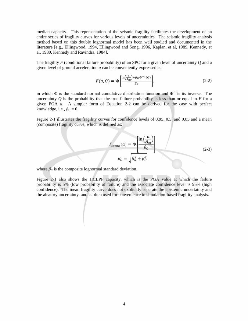
The fragility F (conditional failure probability) of an SPC for a given level of uncertainty Q and a

given level of ground acceleration a can be conveniently expressed as:

( ) * .

/ ( )

+, (2-2)

in which Φ is the standard normal cumulative distribution function and Φ-1

is its inverse. The

uncertainty Q is the probability that the true failure probability is less than or equal to F for a

given PGA a. A simpler form of Equation 2-2 can be derived for the case with perfect

knowledge, i.e., βU = 0.

Figure 2-1 illustrates the fragility curves for confidence levels of 0.95, 0.5, and 0.05 and a mean

(composite) fragility curve, which is defined as:

( ) [

.

/

]

√

(2-3)

where βC is the composite lognormal standard deviation.

Figure 2-1 also shows the HCLPF capacity, which is the PGA value at which the failure

probability is 5% (low probability of failure) and the associate confidence level is 95% (high

confidence). The mean fragility curve does not explicitly separate the epistemic uncertainty and

the aleatory uncertainty, and is often used for convenience in simulation-based fragility analysis.

5

Figure 2-1 Illustration of Fragility Curves

Following the definition in Equation 2-1, the HCLPF capacity can be expressed as:

( ( )), (2-4)

which corresponds to about a 1% probability of failure on the mean curve.

The fragility of an SPC can be developed based on a product of a series of factors, which are

often assumed statistically independent. Accordingly, the median capacity Am can be typically

expressed as a product of a median safety factor and the reference ground acceleration, the former

of which can be further decomposed into multiplication of a median strength factor, an inelastic

energy absorption factor, and a median response factor. Some other presentations may also

include other factors, depending on the specific situation of a given SPC. The corresponding

logarithmic standard deviation can be expressed as:

√

√

(2-5)

where n is the number of factors in the product representation of the fragility.

A fragility curve can also be developed based on computerized simulation, in which finite

element analysis is used to obtain the structural responses. In this approach, a complete set of

random variables need to be determined for the governing limit state(s), and the statistical

parameters for the random variables are defined subsequently. Information required to fully

define the random variables may include the marginal/joint probability distribution, mean,

coefficient of variation, and correlation. Simulation-based seismic fragility analysis also requires

the determination of proper simulation techniques, depending on the accuracy requirement, how

efficiently the structural responses can be obtained, target failure probability, etc. The common

Peak Ground Acceleration or Spectral Acceleration

Co

nd

itio

nal

Pro

bab

ilit

y o

f F

ailu

re

6

techniques include the brutal force Monte Carlo simulation, Latin Hypercube sampling,

importance sampling, and Fekete Point sampling [Nie, et al, 2007]. The uncertainties in this

approach are usually provided in a composite sense, i.e., no distinction between the epistemic

uncertainty and the aleatory uncertainty. Consequently, there is only one resultant fragility curve,

which can be considered as the best estimate (composite or mean) fragility curve, in contrast to

the family of fragility curves as described above for the typical closed form solution.

2.2 Seismic Fragility Analysis of Degraded SPCs

The effect of age-related degradation on the seismic fragility of an SPC is twofold: on the median

capacity and on the uncertainties, with the former being potentially more significant.

Degradation of an SPC, often observed as loss of cross section or cracking, reduces the strength

of the SPC and consequently causes the median fragility to decrease. However, the level of

degradation may not affect the median fragility in a linear fashion, due to the dynamic nature of

the seismic responses and also possibly the nonlinear behaviors of the SPC [Ellingwood and Song,

1996]. Since the degradation phenomena of SPCs have a significant amount of uncertainty and

the knowledge for the development of the degradation models is not perfect, the uncertainty

measures βR and βU increase as the SPCs age.

The seismic fragility of a degraded SPC is a function of time. Using the classical double

lognormal model as an example, the seismic fragility of a degraded SPC can be expressed as the

following general form,

( ) * .

( )/ ( ) ( )

( )+, (2-6)

in which t represents time and the fragility parameters Am, βR, and βU become time-dependent to

represent their instant values at time t. Equation 2-6 is conceptually clear; however, except for

very simple cases, the time-dependent fragility is usually very difficult to be further developed by

analytically determining the time-dependent fragility parameters. In most realistic situations,

these fragility parameters are complex functions of time and may often be defined implicitly.

Therefore, ( ) is more suitable to be developed numerically either at some discrete time

points or at postulated levels of degradations.

When there is a reliable age-related degradation model for the subject SPC, the fragility capacity

can be developed for a prescribed period of time, e.g., 80 years (a potentially extended life

expectation of a nuclear power plant in the U.S.). Figure 2-2 illustrates a series of mean fragility

curves that correspond to a series of specified time points (years). This representation of the

time-dependent fragility can assist a fragility analyst to assess how the deteriorating fragility

capacity progresses with time as the subject SPC degrades and to make better decision on

inspection/maintenance scheduling. Of course, the quality of such a decision depends on how

well the age-related degradation model represents the real degradation environment of the subject

SPC.

7

Figure 2-2 Fragility as A Function of Time

In cases where no reliable degradation models are available, the fragility capacity can be

developed for various levels of degradation. This approach is very useful when degradation data

can be obtained from in-service inspections or maintenance programs. The seismic fragility of an

SPC with an observed level of degradation can be used to update the plant PRA to determine

whether the change of core damage frequency (CDF) due to the decreased fragility is significant

enough to warrant a further action. In addition, once a degradation model can be developed using

the observed data, the series of fragility curves developed for various levels of degradation can be

interpolated to predict the performance of the SPC at different times. This approach lends the

analyst the flexibility in changing the time-dependent degradation model (e.g. for the purpose of

sensitivity study) without repeating the fragility analysis, provided that the initial series of

fragility curves adequately cover the range of degradation for the specified period of time. Figure

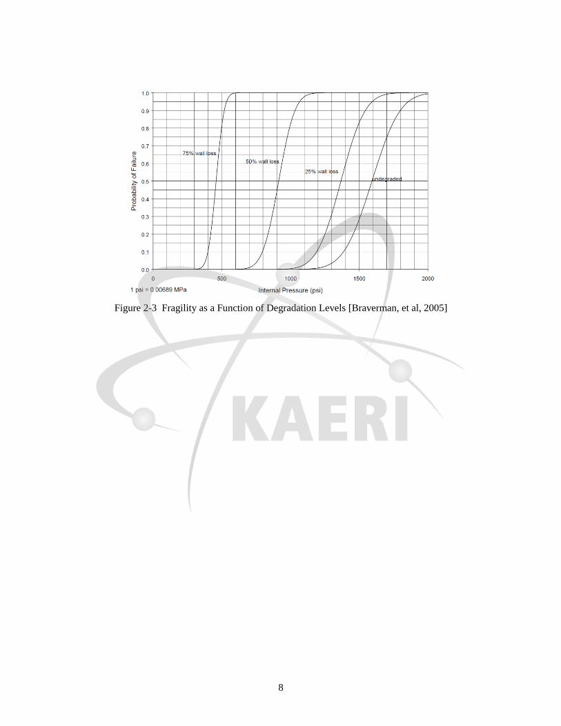
2-3 shows an example of some fragility curves for specified levels of degradation.

From a computational point of view, these two approaches do not differ as significantly as they

appear. Both approaches share a common requirement that the structural strengths need to be

physically reduced, e.g. through reducing the area of a cross section or enlarging a crack. The

first approach that directly integrates time-dependent degradation models usually uses constant

time intervals to determine the levels of cross section loss or the degrees of a crack growth, while

the second approach in general uses a constant spacing to change the same physical parameters.

It should be pointed out that both approaches do not inherently require such constant spacing in

time or in physical parameters; the use of constant spacing is only for better presentation of the

relevant relationships between fragility and time or a physical parameter.

In this report, since the time-dependent degradation models have been selected or developed, the

first approach will be used for the four degradation cases: (A) degraded stainless tank shell, (B)

degraded anchor bolts, (C) anchorage concrete cracking, and (D) a perfect correlation of the three

degradation scenarios. When a more realistic degradation scenario, in which the degradation

cases A, B, and C are not perfectly correlated, is considered, the second approach may be more

suitable because of the requirement of a Monte Carlo or similar simulation. The consideration of

this realistic situation is planned to be part of the Year 4 task.

8

Figure 2-3 Fragility as a Function of Degradation Levels [Braverman, et al, 2005]

9

3 FRAGILITY ANALYSIS OF UNDEGRADED CONDENSATE STORAGE TANK

3.1 The Conservative Deterministic Failure Margin Method

Two methods, namely the conservative deterministic failure margin (CDFM) method and

Fragility Analysis (FA) method were introduced in NUREG/CR-5270 [Kennedy, et al, 1989] to

estimate the seismic margins of structures, systems, and components (SSCs) in nuclear power

plants (NPPs). The seismic margin of a component is defined in these methods as the high

confidence low probability of failure (HCLPF) capacity. The procedure to obtain the HCLPF

capacity of a component requires the estimation of its seismic response as a function of the

seismic margin earthquake (SME) and its seismic capacity. The CDFM method conservatively

prescribes values for the parameters and requires some level of subjective decisions in

formulating the procedures; it produces a deterministic HCLPF capacity. On the other hand, the

FA method requires the determination of the median and the associated uncertainties (βR and βU),

which are under substantial subjective judgment; this method yields an HCLPF capacity as well

as the overall randomness βR and uncertainty βU. The CDFM method was developed for

simplicity based on the FA analysis method, such that the HCLPF capacity can be calculated

deterministically without specifying many subjective parameters. The FA method is based on the

double lognormal model, which is described in Section 2.

In the CDFM method, a set of deterministic guidelines are specified to prescribe the selection of

strength, damping, ductility, load combination, structural model, soil-structural interaction, in-

structural response spectra, etc, in the fragility calculation. This method follows the design

procedures commonly used by the industry, except that some parameters are chosen differently.

It is therefore easy to be implemented and accepted by fragility analysts. The selection of the

parameters is somewhat judgmental to account for the margins and uncertainties. The goal of this

method is to obtain conservative but somewhat realistic HCLPF capacities.

More details on the CDFM method and the FA method can be found in NUREG/CR-5270. Very

similar introduction of the same methods were also included in EPRI NP-6041-SL [Reed, et al,

1991].

3.2 Information of Condensate Storage Tank

The condensate storage tank (CST) to be analyzed in this study was provided by KAERI, in light

of the high contribution of the CST to the core damage frequency. This CST is located in the

Ulchin nuclear power plant, which is located on the east side of Korea on the coast of the Pacific

Ocean. Two CSTs are built close to each other, with a center-to-center separation of 89’ (27.13

m). There is an auxiliary building between the two CSTs, with the roof about 13 feet above the

tank foundation. Figure 3-1 shows a photo of the CSTs and the auxiliary building. The shell

plate, bottom plate, and the roof plate of the tank are SA240-304 stainless steel.

10

Figure 3-1 Photo of the Condensate Storage Tanks [KAERI Email Communication to BNL,

09/29/2009]

Figure 3-2 Elevation View of the Condensate Storage Tank [KEPC Ulchin NPP Unit 3 & 4,

Drawing No. M262-DG-A03-01, Rev. 6]

11

Table 3-1 Key Dimensions of the Condensate Storage Tank

Inner Diameter 50’ (15.24 m)

Tank Height (to water level) 37’-6” (11.43 m)

Shell Thickness 5/8” (15.875 mm)

Torispherical Head Thickness 1/2” (12.7 mm)

Bottom Plate Thickness 1/4”~5/16” (7 mm)

Figure 3-3 Anchor Bolt Orientation [KEPC Ulchin NPP Unit 3 & 4, Drawing No. M262-DG-

A03-01, Rev. 6]

Figure 3-4 Anchor Bolt Chair [KEPC Ulchin NPP Unit 3 & 4, Drawing No. M262-DG-A03-01,

Rev. 6]

12

Figure 3-2 shows an elevation view of the CST. The CST is a flat-bottom cylindrical tank filled

with water and under atmospheric pressure. The key dimensions of the tank are summarized in

Table 3-1. The inner diameter of the tank is 50’ and the height of tank (up to the water level) is

37’-6”. The thickness of the tank shell is 5/8”. Unlike other dimensions in Figure 3-2 that are

shown in both the metric unit and the U.S. customary unit, the thickness of the bottom plate is

only shown in metric unit (7 mm). A corresponding conversion to the U.S. customary unit could

be between 1/4" and 5/16”. Therefore, a thickness of 7 mm will be used in the calculation

because the software that was used in this study can handle mixed units simultaneously. The

radius of the torispherical head is not readily available and neither is its height. Since the

elevation view is provided as part of a scaled design drawing, the missing dimensions of the

torisphere were estimated using measurements of the CST elevation view.

The CST is heavily anchored to the reinforced concrete foundation through 78 anchor bolts. The

anchor bolts have a diameter of 2-1/2” and are A36 steel. Figure 3-3 and Figure 3-4 show a plan

view of the anchor bolt layout and the anchor bolt chair, respectively. The length of the anchor

bolts is 3’-6”, with an embedment of about 2’-1”. The anchor bolts were post-installed in the pre-

formed holes in the concrete foundation with non-shrinking grout. No information about the

strength of the reinforcement concrete and the non-shrinking grout can be found in the drawings

provided by KAERI. However, in an experimental study of the tensile strength of anchor bolts

used for very similar CSTs in another Korean NPP, the compressive strength of the concrete

foundation of the CSTs was specified as 4,500 psi. Therefore, a compressive strength of 4,500

psi was assumed in the fragility analysis of the subject CST. In the test, the actual 7 day and 28

day compressive strengths of the concrete were measured to be 5,419 psi and 7,180 psi,

respectively. The actual compressive strength of the non-shrinking grout was reported to be

7,550 psi and 111,000 psi, respectively, at 7 days and 21 days [Lee, et al, 2001].

KAERI indicated that the tank is founded on a rock site. Therefore, soil-structure interaction (SSI)

is not relevant to the subject CST.

Figure 3-5 Anchor Bolt Embedment [KAERI Email Communication to BNL, 09/29/2009,

Document No. 9-251-C118-002]

13

3.3 Fragility Analysis of the Undegraded CST

A sophisticated procedure to calculate the HCLPF capacity of flat bottom tanks using the CDFM

method is introduced in Appendix A of NUREG/CR-5270 [Kennedy, et al, 1989]. This

procedure involves an extensive set of equations to calculate the seismic responses and seismic

margin capacities. Within the scope of Year 3 work, fragility analysis of the undegraded case

(baseline) as well as a few other cases involving multiple degradation scenarios will be performed.

Each of the degraded cases is further divided into a series of fragility analyses for various levels

of degradation. To accomplish such a large computational effort with the given resources, an

efficient and robust method is necessary. To this end, the mathematical software Mathcad [2007]

was chosen because of: (1) its capability in explicitly expressing mathematical equations in a

fashion that a common engineer is familiar with, (2) its advanced functions in performing

interpolation and root finding without significant programming, (3) its capability in mixing

documentation and calculation so that the necessary technical background and explanations can

be documented, and (4) its instant numerical calculation and plot rendering when any parameters

are varied. The utilization of this tool saved considerable time that would be used in developing

spreadsheet or in-house code, because the clear presentation of equations avoided much

unnecessary debugging time.

The calculation of the HCLPF capacity using the CDFM method follows mostly the

recommendations in NUREG/CR-5270, supplemented with BNL 52361 [Bandyopadhyay, et al,

1995], ASCE 4-98 [1998], NASA SP-8007 [1968], and other references. This section presents a

summary of the analysis and the results; more details can be found in Appendix A of this report.

The CDFM method is an iterative process: (1) a seismic response evaluation is performed for a

given level of estimated seismic margin earthquake SMEe; (2) a seismic capacity assessment is

performed considering the current level of seismic loading to obtain the actual seismic margin

earthquake SME based on the following equation:

(3-1)

in which CAPACITY is the HCLPF capacity of the tank, STATIC is the portion of this capacity

used to resist static loads, kμ is the inelastic energy absorption effective seismic stress correction

factor, and SEISMICe is the seismic response; and (3) steps (1) and (2) are repeated using an

updated SMEe until SME is close to SMEe.

KAERI indicated that the design basis earthquake (DBE) used for the design of the subject CST

was based on NRC Regulatory Guide (RG) 1.60 [1973] design spectrum anchored to a PGA level

of 0.20 g. Therefore, the NRC RG. 1.60 spectrum shapes for the horizontal ground motion and

the vertical ground motion were used for the HCLPF capacity evaluation reported herein. The

median response spectra from NUREG/CR-0098 [Newmark and Hall, 1978] were utilized in the

example reported in Appendix A of NUREG/CR-5270. The RG 1.60 spectra differ from the

median spectra in NUREG/CR-0098 in that the vertical response spectrum is 2/3 of the horizontal

response spectrum not for the entire frequency domain but only for frequencies less than 0.25 Hz.

The RG 1.60 spectrum shapes were implemented in Mathcad using its interpolation function to

automatically determine the spectral acceleration for any given frequency. In addition, the initial

SME estimate is set to 1.67×0.2 g = 0.334 g, in which the factor 1.67 comes from the SRM/SECY

93-087 [1993] requirement that the HCLPF capacity shall be greater than or equal to 1.67 times

the safe shutdown earthquake (SSE) in a margin assessment of seismic events. After several

iterations by trial-and-error, the SME capacity converges to 0.426g, which is used for discussion

14

in the following. Since only the converged SME capacity is used, the repetitive nature of the

CDFM method is effectively omitted in the following discussion.

3.3.1 Seismic Response Evaluation

The weight and the center of gravity (CG) of various parts of the tank were first estimated based

on the dimensions either as shown in Figure 3-2 or as estimated from the same figure. The center

of gravity is defined as its height above the tank bottom plate. As summarized in Table 3-2, the

torispherical head, tank shell, bottom plate, and water weigh 54.5 kips, 157.8 kips, 22.3 kips,

4604.2 kips, respectively. The total weight of the tank including water is 4,839 kips (2195 metric

ton), and the center of gravity is 19.0’ (5.8 m). The water dominates the total weight and the

calculation of the center of gravity. The calculated center of gravity including the tank and water

does not agree with that shown in Figure 3-2 (22’-10 5/8”). However, this CG in the drawing is

close to the center of gravity of the tank only (23.1’). The minor difference may arise from the

estimation of the dimensions of the torispherical tank head.

Table 3-2 Summary of Weights and the Centers of Gravity

Parts Weight (kips/kN) Center of Gravity (ft/m)

Torispherical Tank Head 54.5 / 242.4 42.7 / 13.0

Tank Shell 157.8 / 702.0 19.6 / 6.0

Bottom Plate 22.3 / 99.0 0.0 / 0.0

Water 4604.2 / 20,480.0 18.8 / 5.7

Seismic response evaluation includes the calculation of hydrostatic and hydrodynamic loads on

the tank that is subjected to the earthquake motions at the base of the tank. These responses are

then combined to provide six demand estimates for the HCLPF capacity assessment. These

combined responses are described in the following based on Appendix A of NUREG/CR-5270:

The overturning moment in the tank shell immediately above the base plate of the tank: this

moment is then compared to the base moment capacity, which is governed by a

combination of shell buckling and anchor bolt yielding or failure and often governs the

SME capacity of the tank.

The overturning moment applied to the tank foundation through the tank shell and the base

plate: this moment is only required for tanks founded on soil sites and is generally

determined as part of the SSI analysis. For soil sites, a foundation failure mode should

be investigated. This mode as reported in NUREG/CR-5270 seldom governs the SME

capacity. Since the subject CST is founded on a rock site, the calculation of this

moment and the related capacity is not necessary in this study.

The base shear beneath the tank base plate: this base shear is compared with the horizontal

sliding capacity of the tank. NUREG/CR-5270 reported that for atmospheric tanks with

a radius greater than 15’ (4.6 m), the sliding capacity rarely governs the SME capacity.

However, as will be demonstrated later, the sliding capacity controls the SME capacity

of the subject CST in this study.

The combination of the hydrostatic and hydrodynamic pressures on the tank side wall: The

common design practice is to compare the combined pressures with the membrane hoop

15

capacity of the tank shell at one-foot above the base and each wall thickness change.

Since there is no thickness change in the shell of the subject CST, only one location will

be compared. The combined pressures usually do not control the SME capacity if the

tank is properly designed. However, when degradation of the tank shell is considered,

the combined pressures can govern the SME capacity of the degraded CST.

The average hydrostatic minus hydrodynamic pressure on the base plate of the tank: this

pressure is used to calculate the sliding capacity of the tank. In addition, if fluid hold-

down forces on the base plate are included in the assessment of the overturning moment

capacity, the minimum value of this pressure near the tank side wall is needed.

The fluid slosh height: the slosh height is compared to the freeboard above the water level to

assess the possibility of roof damage. It is noted in NUREG/CR-5270 that roof damage

usually does not affect the safety function of the tank immediately after an earthquake

and is seldom a concern in seismic margin assessment.

Important specifics in the calculation of the HCLPF capacity of the subject CST are described in

the following to facilitate the understanding of Appendix A of this report, where more detailed

calculations can be found.

3.3.1.1 Horizontal Impulsive Mode Response

The natural frequency of the horizontal impulsive mode is a function of the water level height,

tank radius, tank shell thickness, and tank shell material properties. The ratio of the water level to

the tank radius is 1.498, slightly less than the threshold value (1.5) for determination of how the

effective impulsive weight and its center of gravity are calculated. The ratio of the tank shell

thickness to the tank radius is 0.0021. Using Table 7.4 in reference “Seismic Response and

Design of Liquid Storage Tanks,” [Veletos, 1984] and Equation 4.18 in BNL-52631

[Bandyopadhyay, et al, 1995], the horizontal impulsive mode natural frequency was estimated to

be 9.3 Hz.

A 5% of critical damping was recommended in Appendix A of NUREG/CR-5270 as a

conservative estimate of the median damping for the horizontal impulsive mode response. Based

on the RG 1.60 response spectrum anchored to 0.426 g (the converged SME capacity), the

spectral acceleration for the impulsive mode was found to be 1.1 g, equivalent to an amplification

factor of 2.6.

The effective impulsive weight of water and its effective center of gravity (above the bottom plate

of the tank) are calculated to be 3264 kips (14,520 kN) and 14.0’ (4.3 m), respectively. For

determining the effective fluid weight, the tank shell is assumed to be rigid, as recommended per

ASCE 4-98. Accordingly, the impulsive base shear and the moment at the base of the tank shell

were estimated to be 3,838 kips (17,070 kN) and 56,600 kips-ft (76,730 kN-m), respectively. In

addition to the effective impulsive water weight, these impulsive shear and moment also include

the effect of dead weights for the torispherical tank head and the tank shell.

The impulsive hydrodynamic pressure is estimated to be 7.3 psi (50.6 kPa) for a depth

(downward from the water surface) greater than 0.15H (1.7 m). For a depth less than 0.15H, the

impulsive pressure varies linearly from 0 psi to 7.3 psi.

16

3.3.1.2 Horizontal Convective (Sloshing) Mode Response

The natural frequency of the horizontal sloshing mode is a function of the water level height and

the tank radius, and was estimated to be 0.2 Hz. The convective mode is very lightly damped and

the same damping ratio of 0.5% as recommended in NUREG/CR-5270 will be used herein for the

subject CST. Using the sloshing natural frequency 0.2 Hz and a 0.5% damped RG 1.60

horizontal response spectrum anchored at 0.426 g, the spectral acceleration SAC was determined

to be 0.3 g. Since the sloshing natural frequency is smaller than the lowest corner frequency

(point D in RG 1.60 horizontal spectrum), the RG 1.60 spectrum was defined using data point at

0.1 Hz and point D which were obtained from the spectrum shape.

The effective convective mode water weight and its effective application height were estimated to

be 1,402 kips (6,236 kN) and 25.5’ (7.8 m), respectively. Using a spectral acceleration 0.3 g, the

convective base shear and moment are then determined to be 407.8 kips (1,814 kN) and 10,400

kips-ft (14,100 kN-m), respectively.

The hydrodynamic convective pressure, which is a function of depth (downward from the water

surface), was estimated to be 2.6 psi (18.2 kPa) at the water surface and 0.3 psi (2.3 kPa) at the

base of the tank. The hydrodynamic convective pressure is generally smaller at greater depths.

In general, it is negligible compared to either the hydrodynamic impulsive pressure or the

hydrostatic pressure at the base of tank.

The fundamental mode fluid slosh height was estimated to be 6.1 ft (1.9 m), corresponding to a

SME capacity of 0.426 g.

3.3.1.3 Vertical Fluid Mode Response

The alternative method reported in Appendix A of NUREG/CR-5270 and also available in ASCE

4-98 was used to estimate the fundamental frequency of the vertical fluid mode, because the

equations in NUREG/CR-5270 are not applicable to the shell-thickness/radius ratio of the CST

(0.0021). Using Equation C3.5-13 of ASCE 4-98, the fundamental frequency of the vertical fluid

mode of the CST was estimated to be 9.5 Hz, which is slightly greater than the fundamental

frequency of the horizontal impulsive mode. A similar observation was also reached in

NUREG/CR-5270.

A 5% of critical damping was assumed for the evaluation of the vertical spectral acceleration, as

recommended in NUREG/CR-5270. This damping recommendation partially accounted for the

foundation flexibility. Using the RG 1.60 vertical response spectrum anchored to 0.426 g (note:

RG 1.60 horizontal and vertical spectra anchor to the same horizontal PGA), the spectral

acceleration for the vertical mode was determined to be 1.1 g.

The hydrodynamic pressure for the vertical fluid response mode is a function of depth, and is zero

at the water surface. It was estimated to be 14.3 psi at the tank base plate, which is greater than

those due to the horizontal impulsive mode and the horizontal convective mode.

3.3.1.4 Combined Reponses

The horizontal responses due to the horizontal impulsive mode and the horizontal convective

mode can be combined using the squared root of sum of squares (SRSS) method.

For the purpose of the membrane hoop stress capacity check, the maximum seismic

hydrodynamic pressures can be obtained by SRSS of the horizontal seismic pressures and the

17

vertical fluid response hydrodynamic pressure. The maximum seismic hydrodynamic pressure

was found to be 16.0 psi at the tank base plate.

For the purpose of estimating the buckling capacity of the tank shell, it is necessary to estimate

the expected maximum and minimum of the fluid pressures acting against the tank shell near its

base at the location of the maximum axial compression during the time of maximum base

moment. The expected maximum and minimum compression zone pressures PC+ and PC-, were

estimated to be 29.2 psi and 17.9 psi, respectively. These estimates include hydrostatic pressure,

hydrodynamic pressure due to the horizontal fluid response modes, and 40% (see Appendix A) of

the hydrodynamic pressure due to the vertical fluid response mode.

For the purpose of estimating the expected minimum fluid hold-down forces in the zone of

maximum tank wall axial tension, it is required to estimate the minimum tension zone fluid

pressure PT- at the time of maximum moment. PT- was estimated to be 3.2 psi, in a similar way to

the pressures at the compression zone.

For the evaluation of the sliding capacity, the expected minimum average fluid pressure Pa on the

base plate, at the time of the maximum base shear, can be estimated to be 10.5 psi. This pressure

was determined as the hydrostatic pressure less 40% of the hydrodynamic pressure due to the

vertical fluid response mode.

The expected minimum total effective weight WTe of the tank shell acting on the base, at the time

of maximum moment and base shear, can be estimated to be 188.2 kips.

3.3.2 Seismic Capacity Assessment

The seismic capacity assessment requires the determinations of three basic capacities of the tank:

(1) compressive buckling capacity of the tank shell, (2) the tensile hold down capacity of the

anchorage, and (3) the hold-down capacity of the fluid pressure acting on the base plate. Each of

these basic capacities will be discussed below, followed by the discussion of the overturning

moment capacity, sliding capacity, fluid pressure capacity of the tank shell, and other capacities.

In general, the seismic capacity evaluation is more complicated than the seismic response

evaluation.

3.3.2.1 Compressive Buckling Capacity of the Tank Shell

The most likely buckling for tanks is the "elephant-foot" buckling near the base of the tank shell.

The "elephant-foot" buckling is a combined effect of hoop tension, axial (vertical) compression,

and restriction of radial deformation of the tank shell by the base plate. "Elephant-foot" buckling

does not necessarily lead to failure of a tank (e.g. leakage). However, no simple capability

evaluation method exists to predict tank performance after the development of "elephant-foot"

buckling. Therefore, for the evaluation of the SME capacity of tanks, the onset of "elephant-foot"

buckling will be judged to represent the limit to the compressive buckling capacity of the tank

shell. The onset of "elephant-foot" buckling can be estimated using elastic-plastic collapse theory.

The CST shell is SA 204-type 304 stainless steel. This material does not have a flat yield plateau

and as strain increases its stress can grow to a minimum ultimate stress capacity of 75 ksi. In the

CDFM method, an effective yield stress σye is set to 2.4SM or 45 ksi, in line with the ASME

seismic design limit for primary local membrane plus primary bending [ASME 1983, "ASME

Boilder & Pressure Vessel Code"]. The potential uncertainty range for σye was reported to be

between 30 ksi and 60 ksi, according to the original CDFM method description in Appendix A of

NUREG/CR-5270. In this calculation, the effective yield stress took the median value of 45 ksi.

18

The "elephant-foot" buckling axial stress of the tank shell can be accurately predicted to be 21.4

ksi. The compressive buckling capacity for HCLPF capacity computations utilizes a

recommended 0.9 reduction of the buckling stress and was estimated to be 12.1 kips/in.

A check of the buckling capacity of the supported cylindrical shells under combined axial

bending and internal pressure showed that it did not govern the buckling capacity of the CST

shell. This check required the reference NASA SP-8007 [1968] to define parameters and

procedures to compute the buckling capacity under combined axial bending and internal pressure.

Figure 6 of NASA SP-8007 will be digitalized in the next section to automatically determine a

parameter that varies with the degradation state.

3.3.2.2 Bolt Hold-Down Capacity

The bolt hold-down capacity should be determined as the smallest of the bolt tensile capacity,

anchorage of bolt into the concrete foundation, capacity of the top plate of bolt chairs to transfer

bolt loads to the vertical chair gussets, attachment of the top plate and vertical chair gussets to the

tank shell, and the capacity of tank shell to withstand concentrated loads imposed on it by bolt

chairs.

According to the drawing, the anchor bolt chairs form a circumferentially continuous construction.

Based on the continuous chair construction and the sizing of the plates and weld, it is judged that

the anchor bolt chair and its attachment to the tank shell are adequate to transfer the bolt capacity

load for the CST. The tank shell is also considered to be adequate in withstanding the

concentrated loads imposed on it by bolt chairs, especially because the "elephant-foot" buckling

capacity is also checked.

The anchor bolt is A36 steel and has a diameter of 2 1/2". Based on the AISC code [9th edition,

1989], the tensile capacity of the anchor bolt was determined to be 159.4 kips.

The failure of the anchorage of the bolt into the concrete foundation can be bolt failure, plug pull-

out, and concrete cone failure. The tensile capacity of the anchorage is difficult to analyze.

Fortunately, Lee, et al [2001] performed an experimental study of very similar anchor bolts and

anchorages. Based on the test results, the anchorage capacity was about 200 kips, which is about

26% higher than the tensile strength of the anchor bolt. It should be noted that in the test one

specimen had abrasion in its thread, suggesting the anchor bolt capacity should be also close to

200 kips. However, since the embedment in the test was about 1-3/8 inch longer than the subject

CST case, the spacing of anchor bolts in the test is twice as long as in the subject CST case, and

the lab test condition usually have a higher quality control, the bolt hold-down capacity is

assumed to be the bolt tensile capacity 159.4 kips.

3.3.2.3 Fluid Hold-Down Capacity

Figure 3-6 shows a schematic depiction of the relationship among the hold-down tension Te, the

uplift δe, the uplift distance l, the rotation αe, the moment Me, and water pressure P, at the region

of axial tension in tank shell. Based on a small displacement theory, a set of equations were

developed in NUREG/CR-5270 to determine a relation between Te and δe. For unanchored tanks,

it was showed that the fluid hold-down force Te and the uplift δe can be greatly increased if a

large displacement membrane theory had been employed. Nevertheless, for anchored tanks like

the subject CST, the uplift is not expected to be very large. For the small displacement theory to

be applicable, the maximum δe must be less than or equal to 0.6×tB = 0.165”, where tB is the

thickness of the tank bottom plate. Since the hold-down force Te increases as the fluid pressure P

19

increases, the fluid pressure P was conservatively assumed to take the minimum tension zone

fluid pressure PT- = 3.2 psi.

Figure 3-6 Illustration of Tank Bottom Behavior near Tensile Region of Tank Shell [from

NUREG/CR-5270]

Figure 3-7 Relation of Fluid Hold-down Force and Uplift Displacement

Figure 3-7 shows a relationship between the fluid hold-down force and the uplift displacement in

solid line. It should be noted that with no uplift, the fluid hold-down force was non zero (about

19 lbf/in). Beyond the limit of an uplift displacement of 0.165”, the small displacement theory

will be increasingly conservative. A linear approximation of this relationship is also shown in

Figure 3-7, and will be used in the evaluation of overturning moment capacity. This linear

20

approximation was implemented in Mathcad in a highly automated fashion, so that no manual

intervention is needed during the trial-and-error iteration process for the SME capacity evaluation.

An upper limit on the fluid hold-down capacity was assessed based on the assumption of two

plastic hinges at both ends of the uplifted zone of the tank base plate. The upper limit of the fluid

hold-down capacity indicates that the linear approximation of the Te-δe relation shall not be used

beyond δe = 1.07”.

More detailed discussion can be found in Appendix A of NUREG/CR-5270 and Appendix A of

this report.

3.3.2.4 Overturning Moment Capacity

Figure 3-8 Vertical Loading on Tank Shell at Base [from NUREG/CR-5270]

21

The overturning moment capacity can be estimated using the compressive buckling capacity of

the tank shell, the anchor bolt hold-down capacity, and the relationship between fluid hold-down

force and uplift displacement. Several conservative but reasonable assumptions were also made:

(1) the bottom of the tank shell is assumed to rigidly rotate vertically (plane sections remain

plane); (2) the cross-section of the tank right above the top plate of the bolt chairs is assumed to

remain horizontal so that all vertical tank distortions needed to result in base uplift and

mobilization of the anchor bolts must be accommodated below this level; and (3) the compressive

stress varies linearly from zero at the neutral axis (α =β as in Figure 3-8) to its maximum value at

α =180°. Because the bolt pretension is unreliable after a number of years in service, it is

conservatively assumed to be zero.

The neutral axis angle β was determined iteratively by trial-and-error in NUREG/CR-5270, so

that the tank shell compressive buckling capacity was achieved. This study utilized the root

finding function in Mathcad to automate the determination of β; Appendix A of this report

provides more details on the procedure and the technique to determine β. Corresponding to the

converged SME 0.426 g, β was found to be 131.3°. The overturning moment was estimated,

using β and the shell compressive capacity, to be 152,232 kips-ft.

The largest bolt elongation (at α = 0), at the time of the maximum overturning moment, was

estimated to be 0.08%, much smaller than the 1% recommendation for the A307 bolt in Appendix

A of NUREG/CR-5270. It is assumed that A36 bolts and the A307 bolts have a similar

elongation capacity.

The corresponding maximum tank shell uplift distortion was found to be 0.03”, which is much

smaller than the linear limit of 0.165”, and certainly much smaller than the applicability limit of

1.07”.

The study of the example tank in Appendix A of NUREG/CR-5270 needed to consider α = 0 both

at a bolt or in the midway between two adjacent bolts, because there were only 8 anchor bolts tied

the tank to its foundation. On the other hand, the subject CST has 78 anchor bolts, therefore a

case with α = 0 at a bolt is sufficient.

An inelastic energy absorption factor k of unity was conservatively applied in the analysis,

because it is difficult to make an appropriate estimation of K for a hybrid failure mode that

combines bolt yielding and tank shell buckling. At an SME earthquake of 0.426 g, the

overturning moment SME was found to be at a value of 1.1 g, which is significantly higher than

that of the sliding capacity.

3.3.2.5 Sliding Capacity

The base shear and the base overturning moment are primarily due to the horizontal impulsive

mode of fluid response, and their maxima coincide in time. The key in assessment of sliding

capacity is the selection of the coefficient of friction (COF). For the example tank where several

rough steps exist on the surface between the bottom plate and the sand cushion, NUREG/CR-

5270 recommended a COF of 0.70. For flat-bottom steel tanks on concrete foundation, the COF

is estimated to be 0.55 [Bandyopadhyay, et al, 1995]. A COF of 0.55 will be used in this study.

The sliding capacity of the tank cannot take advantage of the shear capacity of the anchor bolts

because (a) there is a large space between the concrete foundation and the anchor bolt chair, and

(b) there is 1/4" diametric clearance in the hole in the anchor bolt chair, and (c) the pretension in

the anchor bolts, if any, are not reliable.

22

It is recommended in NUREG/CR-5270 that the inelastic energy absorption reduction factor to

take a value of unity for the base shear sliding.

The calculated SME capacity for the sliding mode is 0.426 g, and governs the seismic margin

capacity of this tank. This is different from the example tank in NUREG/CR-5270, in which the

overturning moment capacity governs. Had a COF of 0.7 was used, the sliding SME capacity

was calculated as 0.555 g.

3.3.2.6 Fluid Pressure Capacity

The hoop membrane stress capacity was recommended in NUREG/CR-5270 to take the ASME

seismic design limit of 2 SM for primary stress, which is 37.5 ksi for SA240-type 304 stainless

steel. The inelastic energy absorption reduction factor was recommended to be 0.8.

At an SME earthquake of 0.426 g, the estimated HCLPF SME for the fluid pressure mode was

found to be 2.1 g, which is significantly larger than the sliding HCLPF SME capacity.

3.3.2.7 Other Capacity Check

There are a few other capacities that were recommended to check, although they usually do not

govern the SME capacity. In particular for this study, the two CSTs can potentially interact with

the auxiliary building between them, possibly resulting in a lower SME capacity. These checks

are coded in the Mathcad worksheet so that any (unlikely) governing case from these capacities

can be detected.

Slosh height for roof damage: with the HCLPF shear capacity of 0.426 g, the sloshing height

can be about 6.1 ft, which is lower than the total height of the head (8.7', as

approximated in the beginning part of this calculation). It was found during the iteration

process that the increase of sloshing height was not significant as SMEe increased from

0.334 g to 0.426g. In addition, as pointed out in the NUREG/CR-5270, even if roof

damage might occur, such damage usually does not impair the ability of the tank to

contain fluid.

Foundation failure: as indicated by KAERI, the CST founded on a rock site, therefore soil-

tank foundation interaction was not considered.

Piping failure or failure of nozzles: these failures may lead to loss of fluid in the tank, and

more importantly, may impair the normal function of the condensation system. As

reported in NUREG/CR-5270, a significant fraction of the cases of seismic induced loss

of tank contents have been due to piping/nozzle failures because of poor detailing. It is

recommended that an SME evaluation of piping/nozzle failures is necessary only when

poor seismic detailing is found in the involved piping attached to the tank. In this study,

the subject CST is assumed to be appropriately detailed, i.e. the piping and nozzles

directly attached to the tank are properly designed and constructed so that sufficient

piping flexibility can be achieved to accommodate large relative seismic anchor

movements. KAERI also expressed a similar observation on the pipe/nozzle failure in

an email communication.

Interaction of tank-auxiliary building: the influence of the auxiliary building in between the

two CSTs on the SME capacity was assessed in the study. The 3” gap between the roof

of the auxiliary building and the CSTs is filled with elastomeric sealant; there are no

other contact points above the tank foundation (see Figure 3-9 and Figure 3-10).

23

A simplified check was performed by calculating the rotation angle at the tank base and

the maximum horizontal displacement at the roof level. The maximum tank shell uplift

distortion is found to be 0.026 in, which corresponds to a neutral axis angle β of 131.2°.

Since the horizontal plane at the anchor bolt chair is assumed to remain plane and all

distortion is assumed to occur below this level, the rotation angle around the neutral axis

was estimated to be 5.3×10-5

(0.003°). The height of the auxiliary building between the

top of the foundation and the top of the roof is about 13’. The maximum horizontal

displacement at the roof level was estimated to be 0.008” (0.2 mm), which is only about

0.3% of the 3” gap. Based on this result, it is judged that influence of the auxiliary

building on the SME capacity of the CST is minimal.

Figure 3-9 Plan View of CST/Auxiliary Building at Roof Level [KAERI Email Communication

to BNL, 09/29/2009, Document No. 9-251-C118-002]

24

Figure 3-10 Detailing of CST/Roof of Auxiliary Building [KAERI Email Communication to

BNL, 09/29/2009, Document No. 9-251-C118-002]

3.3.3 Summary of the CST Seismic Fragility

The HCLPF SME capacity of the CST was estimated to be 0.426 g, which is governed by the

sliding capacity. At this capacity, the calculated SME’s based on the overturning moment and the

fluid pressure response modes were 1.1 g and 2.1 g, respectively. It should be noted that these

calculated SME’s are not the converged overturning moment SME capacity or the fluid pressure

SME capacity, which require separate iterations to be determined. It is important to emphasize

that the estimated HCLPF SME capacity is conditioned on the RG 1.60 response spectra

anchored to 0.426 g.

This HCLPF SME capacity estimate is very close to the value reported by Choun, et al [2008],

which is 0.41 g and also sliding capacity governs. This good agreement validates the accuracy of

the calculation implemented in Mathcad and provides confidence in the results of the fragility

analysis of degraded CST, which will be introduced in the next section.

Uncertainties βR and βU are required to develop the full fragility of the CST. Since the CDFM

method relies on deterministic but conservative parameters and only yields the HCLPF capacity,

the uncertainties are not available in this analysis. As commonly understood, the uncertainties are

very much subjective; therefore their determination depends on a significant level of expertise,

which may not be readily available through one source or by one person. In this study, a full

examination of the uncertainties associated with the CST was not performed because of the

subjective nature of the uncertainty estimates. Instead, the uncertainties in various parameters,

especially the resultant uncertainties associated with the median fragility of the example tank in

NUREG/CR-5270, were used directly, because these two tanks are similar in size and materials.

As reported in Appendix A of NUREG/CR-5270 in the FA method, the aleatory uncertainty βR

and the epistemic uncertainty βU were 0.20 and 0.27, respectively. These uncertainty values are

almost identical to those reported by Choun, et al [2008], where the only difference is that the

aleatory uncertainty was 0.21. The composite uncertainty βC can be calculated as 0.34.

Based on the HCLPF capacity and the uncertainties, the median fragility capacity can be

estimated to be 0.923 g. Figure 3-11 shows the mean fragility curve and the median, 5%

25

percentile, and 95% percentile fragility curves. Figure 3-12 shows a 3-dimensional view of the

fragility of the CST as a function of the controlling variable PGA and the confidence level Q.

Figure 3-11 Fragility Curves of the CST

Figure 3-12 A 3D View of the CST Fragility as a Function of PGA and Confidence Level Q

26

The Mathcad worksheet for the fragility analysis of the undegraded CST was modified to

incorporate various degradation scenarios and the results of these time-dependent fragility

analyses will be documented in the next section.

27

4 FRAGILITY ANALYSIS OF DEGRADED CONDENSATE STORAGE TANK

BNL performed a series of time-dependent fragility analyses of the CST by incorporating

selected aging-related material degradation models into the fragility analysis. Three separate

degradation scenarios and one combined degradation scenario were considered: (A) degraded

stainless tank shell, (B) degraded anchor bolts, (C) anchorage concrete cracking, and (D) a perfect

correlation of the three degradation scenarios. As agreed with KAERI, the degradation scenarios

A and B will use degradation models from the Year 2 report for demonstration purposes, with a

best effort in determining the required parameters. In degradation scenario C, a hybrid

degradation model was developed based on available anchorage test results for cracked concrete

and KAERI’s recent regression model/data that utilized measurements from Korean NPPs. The

recorded degradation data were very valuable because such data are not commonly available.

The degradation scenario D considers all three degradation cases A, B, and C together, assuming

a perfect correlation among them.

This section describes for each of the four cases the selected degradation model, determination of

parameters, fragility analysis for the degraded CST, and the results from these analyses. More

specifics can be found in Appendices B through E. It should be noted that these appendices were

developed based on the undegraded case, and therefore some portion of the analysis that is not

specifically important to the degraded cases, such as the weight and the frequency calculation, is

omitted (hidden, in the Mathcad terms) for simplicity.

4.1 Fragility Analysis for (A) Degraded Tank Shell

4.1.1 Degradation Model for Stainless Steel Tank Shell

The material degradation model for the stainless steel tank shell to be used in this study is the

mechanochemical model for stress corrosion cracking (SCC), which is one of the three time-

dependent material degradation models for stainless steel that are documented in the Year 2

annual report [Nie, et al, 2009]. It is noticed from Figure 3-1 that there are no signs of significant

degradation in the CST shell, therefore, the consideration of tank shell degradation in fragility

analysis in this section of the report is for the purpose of demonstration. SCC is assumed to be

the degradation mechanism that will be considered for the subject CST.

The mechanochemical model [Saito and Kuniya, 2001] was developed to predict the SCC growth

in stainless steel components submerged in 288 °C water. This model was judged to be relevant

in the NPP environment because austenitic stainless steel (especially type 304) is widely used in

light water reactors (LWRs) and in particular for the subject CST. The structural integrity of the

involved components due to inter-granular stress corrosion cracking (IGSCC) is often a concern

in NPPs. Since the water temperature in the CST is similar to the atmospheric temperature at the

site, the use of this model will demonstrate its application even though the parameters were

chosen to alleviate the effect of high temperatures (which do not exist in this case).

This SCC crack growth model for type 304 stainless steel is based on a hypothesis of the slip-

formation/dissolution mechanism and is expressed as a function of material conditions, water

chemistry, and stress related parameters. This model involves two major mechanisms: 1) slip

step formation due to dislocation movement at the crack tip, and 2) anodic dissolution at the bare

surface after the slip deformation. The derivation of this model was lengthy, highly theoretical,

and beyond the capability of common structural engineers. Interested readers are recommended

to refer back to the original reference. Fortunately, based on the theoretical development, a

relatively simple numerical model was also developed for type 304 stainless steel in 288 °C water,

using a minimal number of parameters [Saito and Kuniya, 2001].

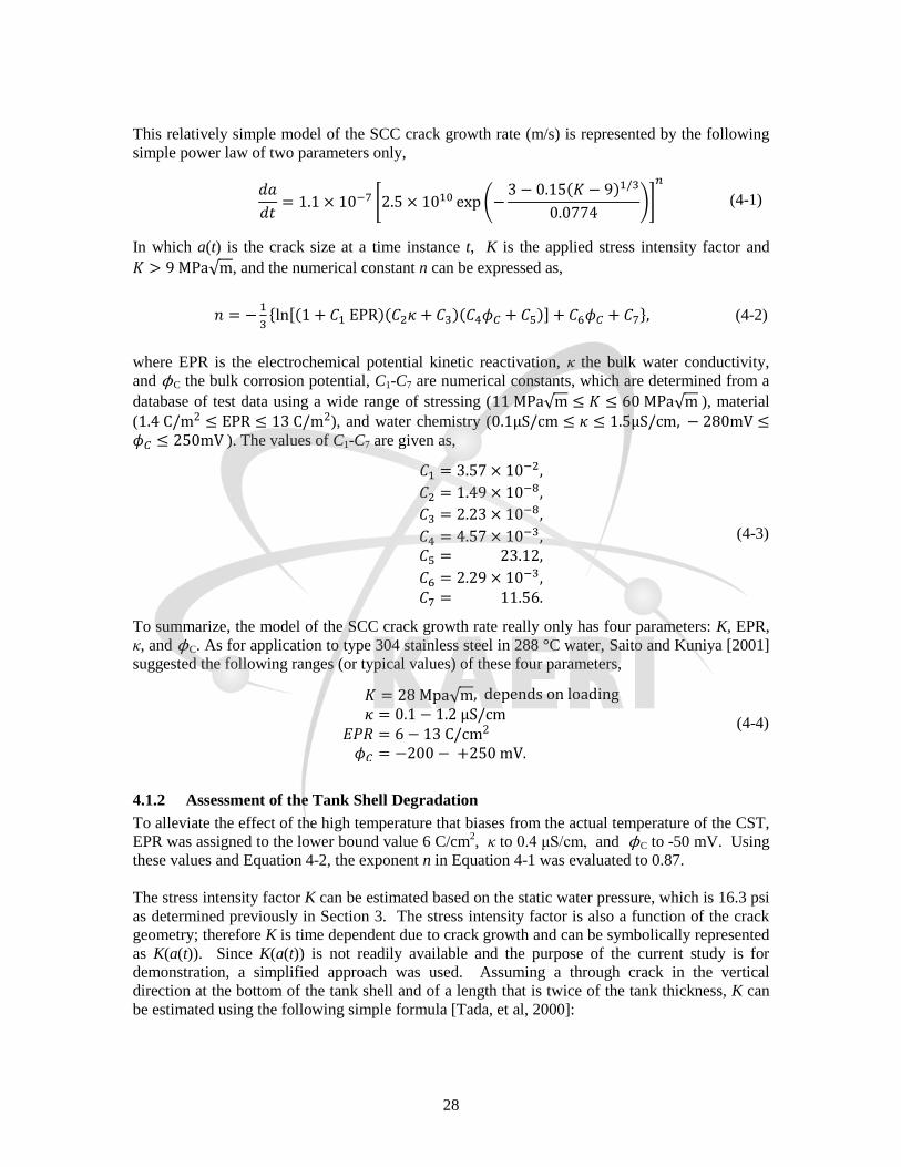
28

This relatively simple model of the SCC crack growth rate (m/s) is represented by the following

simple power law of two parameters only,

* (

( )

)+

(4-1)

In which a(t) is the crack size at a time instance t, K is the applied stress intensity factor and

√ , and the numerical constant n can be expressed as,

* ,( )( )( )- + (4-2)

where EPR is the electrochemical potential kinetic reactivation, κ the bulk water conductivity,

and ϕC the bulk corrosion potential, C1-C7 are numerical constants, which are determined from a

database of test data using a wide range of stressing ( √ √ ), material

( ), and water chemistry ( ). The values of C1-C7 are given as,

(4-3)

To summarize, the model of the SCC crack growth rate really only has four parameters: K, EPR,

κ, and ϕC. As for application to type 304 stainless steel in 288 °C water, Saito and Kuniya [2001]

suggested the following ranges (or typical values) of these four parameters,

√

(4-4)

4.1.2 Assessment of the Tank Shell Degradation

To alleviate the effect of the high temperature that biases from the actual temperature of the CST,

EPR was assigned to the lower bound value 6 C/cm2, κ to 0.4 μS/cm, and ϕC to -50 mV. Using

these values and Equation 4-2, the exponent n in Equation 4-1 was evaluated to 0.87.

The stress intensity factor K can be estimated based on the static water pressure, which is 16.3 psi

as determined previously in Section 3. The stress intensity factor is also a function of the crack

geometry; therefore K is time dependent due to crack growth and can be symbolically represented

as K(a(t)). Since K(a(t)) is not readily available and the purpose of the current study is for

demonstration, a simplified approach was used. Assuming a through crack in the vertical

direction at the bottom of the tank shell and of a length that is twice of the tank thickness, K can

be estimated using the following simple formula [Tada, et al, 2000]:

29

√ √

(4-5)

Based on Equation 4-1, a constant K leads to a constant crack growth rate of 0.0075 in/year. A

list of crack depths can then be calculated for a period of 80 years, which is the current

expectation of the longest operating life of NPPs. Figure 4-1 shows the change of SCC depth as a

function of time (year) and the corresponding wall thinning of the tank shell. Since a few isolated

cracks in the tank shell may not affect much the seismic capacity of the tank, it is further assumed

that many cracks cluster at a small region at the base of the tank shell and the effect of the crack

assembly is similar to loss of material in that location. The fragility analysis of CST with levels

of tank shell degradations will follow this assumption.

Figure 4-1 Change of Tank Shell Thickness/SCC Depth with Time

4.1.3 Fragility Assessment of CST with Degraded Tank Shell

The Mathcad worksheet for the undegraded CST, also designated as the base case, was modified

to incorporate the degradation model for the stainless tank shell. A new variable for the thickness

of tank shell was created separately to track the degradation process. The smaller thickness due

to loss of material is assumed to occur at local regions at the base of the tank shell, and therefore

only the capacity calculation but not the frequency and the response calculation will be changed.

Because of this change of thickness of the tank shell, the upper bound check of the compressive

buckling capacity requires the digitalization of the Figure 6 of NASA SP-8007 and

implementation of an automatic interpolation to determine the necessary parameters. More

details on the update of Mathcad worksheet can be found in Appendix B of this report. It should

be noted that some portion of the calculation and documentation was hidden in Appendix B

because there is no change in that portion and some of the documentation may not be updated

from the base case to minimize the calculation effort.

The direct impact of degraded tank shell is on the compressive buckling capacity and the fluid

hold down capacity, but obviously not on the bolt hold down capacity. All three major resultant

capacities: the overturning moment capacity, sliding capacity, and the fluid pressure capacity are

30

affected. Both the slosh height and the horizontal displacement at the roof level of the auxiliary

building become smaller as the SME becomes smaller due to degradation. These decreases are

because of the decrease in the SME capacity of the CST. Given the same level of input

earthquake the slosh height would be unchanged and the horizontal displacement at the roof level

of the auxiliary building would increase as the level of degradation increases.

Only mean fragility curves will be presented in this report because it is difficult to present the

family of median fragility curves in a plot for more than one degradation level unless utilizing 3D

surfaces such as in Figure 3-12. Even with 3D surfaces, it will be difficult to interpret the 3D

fragility data without an interactive tool because of surface overlapping.

Figure 4-2 shows the mean fragility capacity of the CST with degraded tank shell for a series of

years, from 0 up to 60 years, after which the fragility calculation was not mathematical

achievable. These mean fragility curves were calculated using unchanged uncertainties, i.e., βR =

0.2 and βU = 0.27, the same as utilized for the base case. In reality, since the degradation process

is highly random and uncertain, both the epistemic and aleatory uncertainties should vary with

time. However, reliable uncertainty data on the degradation model were not available to be

utilized. Provided the uncertainty data are available, the updated uncertainties, as functions of

time, can be updated based on Equation 2-5, and these mean fragility curves can be updated

without any technical difficulty. Since the objective of this study is for demonstration purposes,

the effect of the degradation on the uncertainties is not considered. In Figure 4-2, it is obvious

that the spacing of the fragility curves suddenly increases significantly after 45 years, when the

governing failure mode shifted from the sliding failure to the overturning moment failure.

Figure 4-2 Mean Fragility Capacity of the CST with Degraded Tank Shell

31

It is easier to see the transition of failure mode by the relation of the HCLPF fragilities / the

median capacities and time. Figure 4-3 and Figure 4-4 show in solid lines the HCLPF fragilities

and the median capacities of the CST as a function of time, respectively. These figures also

included the corresponding overturning moment capacities, sliding capacities, and the fluid

pressure capacities, in dotted, dashed, and dash-dot lines, respectively. The fragility capacity is

taken as the minimum of these three capacities. It should be noted that the non-governing

capacities are higher than the corresponding real fragility capacities, which require separate

iterations to be determined. From these figures, it is obvious that the tank shell degradation (wall

thinning) has the most significant impact on fluid pressure capacity and the least impact on

sliding capacity. The fragility capacity (either HCLPF capacity or the median capacity) is clearly

dominated by the sliding mode until slightly after 45 years, and then by the overturning mode.

Although the fluid pressure mode does not dominate the fragility capacity up to 60 years, it would

be dominant shortly after 60 years had the calculation continued.

Figure 4-3 HCLPF Capacity of the CST with Degraded Tank Shell

32

Figure 4-4 Median Capacity of the CST with Degraded Tank Shell

4.2 Fragility Analysis for (B) Degraded Anchor Bolts

4.2.1 Degradation Model for Anchor Bolts

Unlike the stainless steel tank shell of the CST, the anchor bolts made of A36 are prone to

corrosion because of the salty moisture in a location close to the ocean. The protecting stainless

steel cover as shown in Figure 3-1 is assumed not to be leak-tight. The power model for steel

corrosion was chosen for modeling the degradation of the anchor bolts, from the Year 2 annual

report [Nie, et al, 2009]. This model had been used by Mori [2005] in a study of reliability-based

service life prediction, which provides a direct indication of its applicability in fragility analysis.

The power model can be used for modeling of both concrete cracking/reinforcement corrosion

and corrosion of carbon and low alloy steel. This model is briefly introduced in the following and

the parameters in the model are then defined.

The depth of corrosion in the power model can be represented by,

( ) (4-6)

in which t is the elapsed time in years, C the rate parameter, and α the order of the power model

that depends on the nature of the attack. The corrosion rate C is a function of material, ambient

moisture, and temperature. The parameters C and α can be estimated using experiments. Table

4-1 shows the average values for these parameters determined by Albrecht and Naeemi [1984].

The level of attack X(t) applicable to this table is in units of μm, and the time t is in years.

33

Since the Ulchin NPP, where the subject CST is installed, is located on the coast, the marine

environment in Table 4-1 was assumed in the fragility analysis of the CST for degraded anchor

bolts, i.e., C = 70.6 and α = 0.79.

Table 4-1 Average Values for Corrosion Parameters C and α [Albrecht and Naeemi, 1984].

Environment Carbon Steel Weathering Steel

C α C α

Rural 34.0 0.65 33.3 0.50

Urban 80.2 0.59 50.7 0.57

Marine 70.6 0.79 40.2 0.56

Based on the power model and the selected parameters C and α, the depth of corrosion of the

anchor bolt is shown in Figure 4-5 as a function of the time in years. Albeit the nature of the

model is nonlinear, the actual depth of the corrosion for this particular application is close to a

linear relation with time.

Figure 4-5 The Depth of Corrosion of the Anchor Bolts

4.2.2 Fragility Assessment of CST with Degraded Anchor Bolts

Similar to degradation case A, the Mathcad worksheet for the base case fragility analysis was

modified to incorporate the degradation model for the A36 anchor bolts. A new variable for the

diameter of the anchor bolts was created separately to track the degradation process. A reduction

of bolt diameter was assumed uniformly for all anchor bolts, as given by,

( ). (4-7)

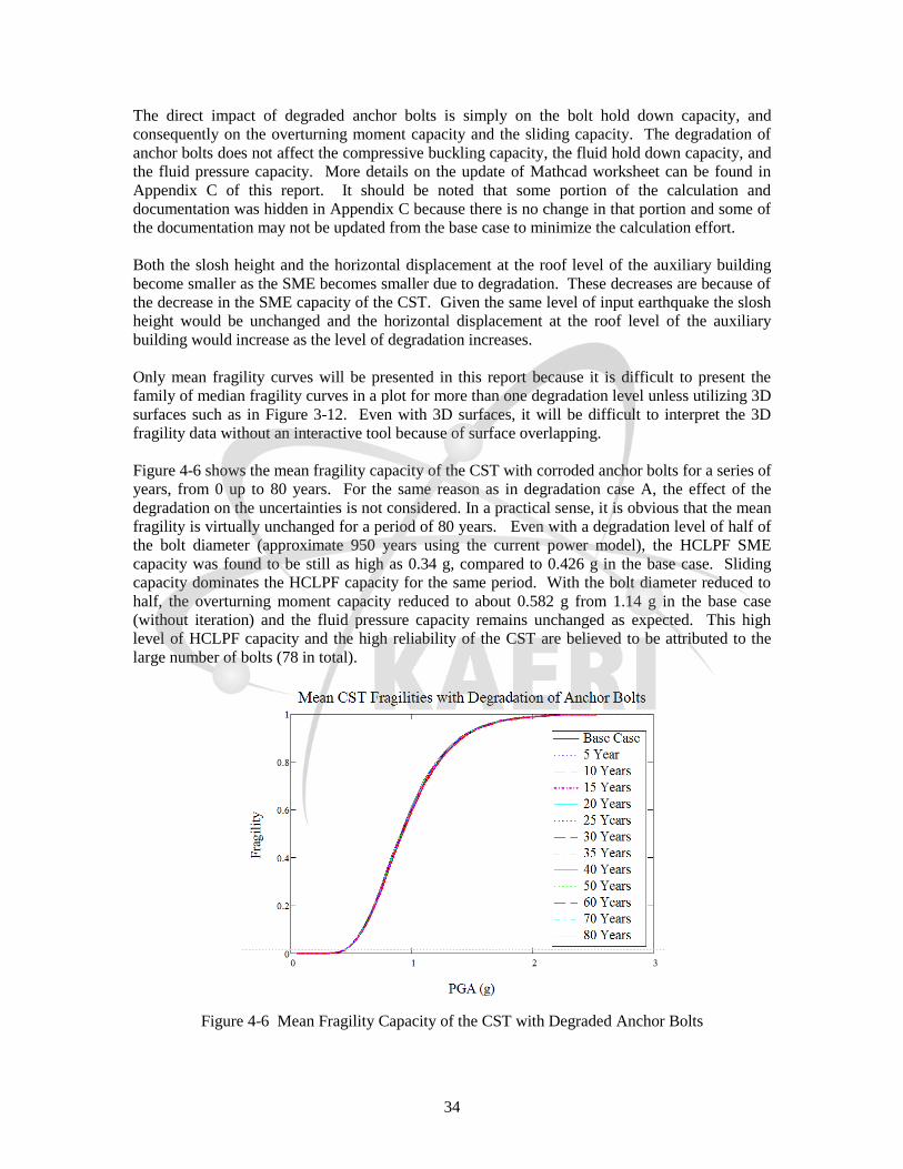
34

The direct impact of degraded anchor bolts is simply on the bolt hold down capacity, and

consequently on the overturning moment capacity and the sliding capacity. The degradation of

anchor bolts does not affect the compressive buckling capacity, the fluid hold down capacity, and

the fluid pressure capacity. More details on the update of Mathcad worksheet can be found in

Appendix C of this report. It should be noted that some portion of the calculation and

documentation was hidden in Appendix C because there is no change in that portion and some of

the documentation may not be updated from the base case to minimize the calculation effort.

Both the slosh height and the horizontal displacement at the roof level of the auxiliary building

become smaller as the SME becomes smaller due to degradation. These decreases are because of

the decrease in the SME capacity of the CST. Given the same level of input earthquake the slosh

height would be unchanged and the horizontal displacement at the roof level of the auxiliary

building would increase as the level of degradation increases.

Only mean fragility curves will be presented in this report because it is difficult to present the

family of median fragility curves in a plot for more than one degradation level unless utilizing 3D

surfaces such as in Figure 3-12. Even with 3D surfaces, it will be difficult to interpret the 3D

fragility data without an interactive tool because of surface overlapping.

Figure 4-6 shows the mean fragility capacity of the CST with corroded anchor bolts for a series of

years, from 0 up to 80 years. For the same reason as in degradation case A, the effect of the

degradation on the uncertainties is not considered. In a practical sense, it is obvious that the mean

fragility is virtually unchanged for a period of 80 years. Even with a degradation level of half of

the bolt diameter (approximate 950 years using the current power model), the HCLPF SME

capacity was found to be still as high as 0.34 g, compared to 0.426 g in the base case. Sliding

capacity dominates the HCLPF capacity for the same period. With the bolt diameter reduced to

half, the overturning moment capacity reduced to about 0.582 g from 1.14 g in the base case

(without iteration) and the fluid pressure capacity remains unchanged as expected. This high

level of HCLPF capacity and the high reliability of the CST are believed to be attributed to the

large number of bolts (78 in total).

Figure 4-6 Mean Fragility Capacity of the CST with Degraded Anchor Bolts

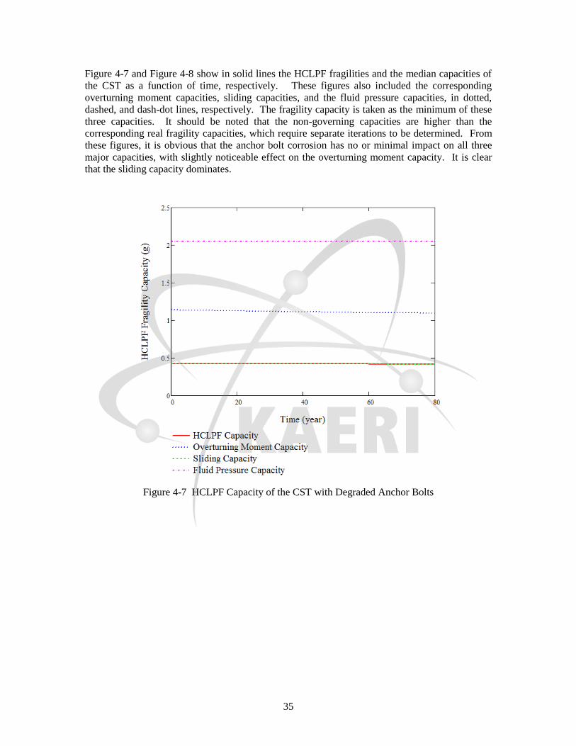
35

Figure 4-7 and Figure 4-8 show in solid lines the HCLPF fragilities and the median capacities of

the CST as a function of time, respectively. These figures also included the corresponding

overturning moment capacities, sliding capacities, and the fluid pressure capacities, in dotted,

dashed, and dash-dot lines, respectively. The fragility capacity is taken as the minimum of these

three capacities. It should be noted that the non-governing capacities are higher than the

corresponding real fragility capacities, which require separate iterations to be determined. From

these figures, it is obvious that the anchor bolt corrosion has no or minimal impact on all three

major capacities, with slightly noticeable effect on the overturning moment capacity. It is clear

that the sliding capacity dominates.

Figure 4-7 HCLPF Capacity of the CST with Degraded Anchor Bolts

36

Figure 4-8 Median Capacity of the CST with Degraded Anchor Bolts

4.3 Fragility Analysis for (C) Cracked Anchorage Concrete

4.3.1 Degradation Model for Cracked Anchorage Concrete

KAERI identified data regarding the crack width and depth of reinforced concrete that were in

four Korean NPPs over a period of about 25 years. Time-dependent models based on regressions

of these data were also provided by KAERI, as shown in Figure 4-9 and Figure 4-10. The linear

crack width model, as reproduced in the following, was used for the fragility analysis of the CST

with cracked anchorage concrete:

( ) , (4-8)

In which W(t) is the crack width (mm) and time t is in years. Since the impact of this model on

the fragility capacity of the CST with cracked anchorage concrete was found to be marginal, a

revised version of this model was developed using the same measurements, by disallowing the

intercept in the linear regression equation. The original version provided by KAERI is designated

as C-1, while the new model is designated as C-2. As shown in Figure 4-11, the new model C-2

can be simply expressed as,

37

( ) , (4-9)

with the same units as in Equation 4-8. It should be pointed out that the measured crack widths

have significant variation and the linear regression models do not necessarily represent true

underlying relationships. The use of these curves in this study is for the purpose of demonstration;

the applicability of these models in practice should be investigated with careful scrutiny.

Figure 4-9 Crack Depth Models Based on Measurements in Korean NPPs (Courtesy of KAERI)

38

Figure 4-10 Crack Width Models Based on Measurements in Korean NPPs (Courtesy of KAERI)

Figure 4-11 New Crack Width Model Based on Measurements in Korean NPPs

The crack width models must be mapped to the anchorage strength for its application to the

fragility analysis of the CST with cracked anchorage concrete. Klingner, et al [1998] developed

an empirical anchor strength – crack width relation for grouted anchors:

y = 0.0078x

0.00

0.05

0.10

0.15

0.20

0.25

0 5 10 15 20 25 30

Cra

ck W

idth

(mm

)

Time (years)

39

√

, (4-10)

where k is a constant determined from test that represents the normalized tensile capacity, heff the

effective embedment (in), P observed tensile capacity (lbf), and is the tested concrete

compressive strength. The grouted anchors reported in NUREG/CR-5434 [Klingner, et al, 1998]

had a diameter of ¾”, an embedment of 4”, and an effective embedment of 4”, which are much

smaller than those of the anchor bolts for the subject CST. For the anchorage construction of the

subject CST, heff was estimated to be 23” by subtracting 1” from the total embedment length to

account for the nut. The concrete nominal compressive strength for the subject CST was

unknown but was assumed to be 4,500 psi according to an experiment by Lee, et al [2001], which

appeared to target at a CST very much similar to the subject CST. The measured concrete and

grout compressive strength were much higher than 4,500 psi in the test; however, since the use of

the nominal compressive strength had already led to a much higher anchor tensile strength, as to

be shown later in this section, than the test results reported by Lee, et al [2001], these measured

strengths were not utilized.

Grout plug pullout is the most dominant failure mode for the anchor bolts under tensile loads,

therefore the friction between the concrete and the grout is crucial in determining the tensile

capacity of the anchor bolts [Lee, et al, 2001, Klingner, et al, 1998]. As shown in Figure 5.20 of

NUREG/CR-5434, the dynamic tensile capacity is higher than the static capacity for uncracked

concrete/grout, while for cracked concrete/grout, the dynamic tensile capacity is lower than the

static capacity. Comparing cracked to uncracked conditions, the reduction in dynamic tensile

capacity was 73% while the reduction in static tensile capacity was 41%. The data for dynamic

load capacity will be utilized for the seismic fragility assessment of the CST. The typical

normalized tensile strength k is 57 for uncracked case and 12.5 for cracked case. The artificial

crack in the test had a width of 0.3 mm (0.012”).

The tensile strength of the anchorage for uncracked case was estimated to be 421.8 kips based on

Equation 4-10, which is much higher than the capacity of 200 kips that was reported by Lee, et al.

[2001]. The reason for this difference may be the substantial difference in the scales of the

anchor bolts in the two test studies; smaller scale usually leads to higher strength as commonly

observed. Therefore, the test data in NUREG/CR-5434 will be used as factors to scale the test

data reported by Lee, et al. [2001]. For the subject CST, the tensile capacity of the anchorage for

a crack width of 0.3 mm can be estimated as 200 kips × 15.5 / 57 = 54.4 kips. The tensile

capacity of the anchorage for a crack width of w mm can be estimated based on the following

linear inter/extrapolation:

( ) kips. (4-11)

In the calculation, T is set to 0 kips as a lower bound value when Equation 4-11 results in an

impractical negative tensile strength. Multiple cracks at one anchor bolt location were not

considered in NUREG/CR-5434 and were not assumed in this study as well.

The smaller of the tensile strength of the anchorage determined using Equation 4-11 and the

anchor bolt tensile capacity becomes the anchor bolt hold-down capacity.

The impact of the cracked concrete is directly on the bolt hold-down capacity but not the tank

shell buckling capacity and the fluid pressure capacity; the overturning moment capacity and the

40

sliding capacity are affected as a consequence. More details on the implementation can be found

in Appendices D and E, which differ only in the crack width model. The crack width model C-1

as provided by KAERI was used in the development of Appendix D, while the newly developed

crack width model C-2 was used in Appendix E.

4.3.2 Fragility Assessment of CST with Cracked Anchorage Concrete

4.3.2.1 Using C-1 Crack Growth Model

Figure 4-12 shows the mean fragility capacity of the CST with cracked anchorage concrete for a

series of years, from 0 up to 80 years. For the same reason as in degradation case A, the effect of

the degradation on the uncertainties is not considered. Figure 4-13 and Figure 4-14 shows the

HCLPF SME capacity and the median SME capacity, respectively. In a practical sense, it is

obvious that all fragility capacities are virtually unchanged for a period of 80 years. The fragility

capacity starts to slightly decrease after 60 years and reaches a HCLPF SME capacity of 0.423 g

at the end of 80 years, which is almost unchanged from the base case of a 0.426 g HCLPF

capacity. Sliding capacity dominates the fragility capacity for the entire period of 80 years. The

overturning moment capacity varied similarly to the sliding capacity, while the fluid pressure

capacity remained unchanged.

At the end of 80 years, the bolt hold-down capacity reduced to 101.2 kips from 159.4 kips at the

base case, representing a 37% reduction. Such a large reduction in the bolt hold-down capacity

did not lead to a comparable level of reduction in fragility capacities because of the large number

of anchor bolts (78). The detailed results can be found in Appendix D.

Figure 4-12 Mean Fragility Capacity of the CST with Cracked Anchorage Concrete (C-1)

41

Figure 4-13 HCLPF Capacity of the CST with Cracked Anchorage Concrete (C-1)

Figure 4-14 Median Capacity of the CST with Cracked Anchorage Concrete (C-1)

42

4.3.2.2 Using C-2 Crack Growth Model

To investigate the sensitivity of the fragility capacities on the degradation model, the newly

developed crack width model C-2 was employed in place of the C-1 model, as shown in

Appendix E.

Figure 4-15 shows the mean fragility capacity of the CST with degraded tank shell for a series of

years, from 0 up to 80 years. Similarly to the previous cases, these mean fragility curves were

calculated using unchanged uncertainties, i.e., βR = 0.2 and βU = 0.27, and the effect of the

degradation on the uncertainties is not considered. In Figure 4-15, the mean fragility does not

change in the first 20 years and in the last 25 years, with an increasing rate of fragility capacity

deterioration for the years in the middle. The governing failure changed from the sliding mode to

overturning moment mode at 50 years.

Figure 4-15 Mean Fragility Capacity of the CST with Cracked Anchorage Concrete (C-2)

43

Figure 4-16 HCLPF Capacity of the CST with Cracked Anchorage Concrete (C-2)

44

Figure 4-17 Median Capacity of the CST with Cracked Anchorage Concrete (C-2)

The deterioration of fragility capacities as a function of time can be easily observed in the HCLPF

fragility and the medina fragility, as shown in Figure 4-16 and Figure 4-17. There are 4 regions

in these figures: (1) during 0-20 years, with a maximum crack width of 0.156 mm (about half of

the crack width in the test), the fragility capacities were unchanged because of the large number

of bolts that have no or moderate reduction in their bolt hold-down capacity; (2) between 20 to

about 48 years, the fragility capacities were dominated by the sliding mode; (3) before 55 year,

the fragility capacities were dominated by the overturning moment mode and the reduction in the

bolt hold-down capacity affect the overturning moment capacity; and (4) after 55 years, the

fragility capacities continue to be dominated by the overturning moment capacity, the bolts in

tension appeared to have been pulled out, and the CST effectively becomes an unanchored tank.

The overturning moment capacity starts to be affected dramatically by the bolt hold-down

capacity after 20 years until the bolts reach a zero capacity around 55 years. The bolt hold-down

capacity does not have as great an impact on the sliding capacity as on the overturning moment

capacity, and it does not have any impact on the fluid pressure capacity as expected.

The fragility capacity is taken as the minimum of these three capacities. It should be noted that

the non-governing capacities are higher than the corresponding real fragility capacities, which

require separate iterations to be determined.

The slosh height become smaller as the SME becomes smaller due to degradation. The horizontal

displacement at the roof level of the auxiliary building becomes larger at the end of years (also

some other years prior to 80 years) than the base case due to the pull out of the anchor bolts and

the CST becomes unanchored. Even in such a case, the largest horizontal displacement at the

45

roof level of the auxiliary building was found to be 0.314”, about 10% of the 3” gap. This could

cause a complication of the failure mode of the CST, and will remain as a recommendation for

future study.

From this sensitivity analysis, the crack growth model has a great impact on the fragility

capacities of the CST. However, the model C-2 may not be accurate after about 40 years because

the crack width becomes greater than 0.3 mm and the crack width estimate after 40 years is

extrapolated. On the other hand, the model C-1 has a maximum crack width of 0.204 mm at the

end of 80 years, which is still in the tested range. It is important to note that provided the linear

inter/extrapolation relation in Equation 4-11 is reasonable, a crack width of 0.429 mm at the end

of 55 years, based on the model C-2 prediction, indicates a pull-out failure of the anchor bolts and

a 61% reduction in seismic fragility capacity, even with a very dense array of anchor bolts (78).

This observation shows the importance of concrete cracking in the CST seismic safety, and

certainly leads to a recommendation of regular inspection of the concrete foundation for cracking.

It is cautioned that the above observation is based on a greatly simplified conversion from the

NUREG/CR-5434 test results to the large size anchor bolts, in which many uncertain factors were

not considered, for example, how the crack depth in conjunction with the crack width affect the

bolt hold-down capacity. As discussed in the Year 2 Annual Report, the surface crack may not

always be a good indicator of the crack depth.

4.4 Fragility Analysis for Multiple Degradations

Degradation cases A, B, and C-2 were combined together to investigate the effect of multiple

degradations on the seismic fragility capacities. The three degradations cases are assumed to be

perfectly correlated, i.e., the severity of each of the degradation case is a deterministic function of

the common time variable. The detailed implementation is presented in Appendix F, which

combines the updates in Appendices B, C, and E. Concrete cracking model C-2 was chosen

instead of model C-1 in order to obtain more interesting fragility results.

Figure 4-18 shows the median fragility curves for the CST with combined degradations up to 65

years. The fragility curves before the end of 45 years show equal and fine spacing between them,

indicating a steady but slow degradation process. Between 45 years and 55 years, a sudden

increase of the degradation severity is shown by the large spacing between the corresponding

fragility curves. The very small spacing between 55 and 60 years suggest a very small drop in the

fragility capacity, followed by a slightly increased drop in fragility capacity. As shown in Figure

4-19, the fragility capacity diminishes at 65 years, after which the fragility calculation in Mathcad

could not reach a plausible solution.

The trend of the fragility capacity change can be better characterized by the HCLPF fragility

capacity and the median fragility capacity, as shown in Figure 4-19 and Figure 4-20. Before the

end of 45 years, the fragility capacity is dominated by the slow deterioration of the sliding

capacity. Between 45 years and 55 years, the dominating failure mode switches to the

overturning moment mode and the resultant deterioration rate in the fragility becomes higher.

Between 55 and 60, the fragility capacity is still dominated by the overturning moment capacity,

which levels to a small constant because the CST effectively is unanchored tank as previously

shown in the degradation case C-2. At the end of 65 years, the overturning moment capacity and

the fluid pressure capacity are very close with the later dominates the fragility capacity. This is

the only occasion among all degradation scenarios that the fluid pressure capacity dominates the

fragility calculation.

46

Figure 4-18 Mean Fragility Capacity of the CST with Combined Degradations

Figure 4-19 HCLPF Capacity of the CST with Combined Degradations

47

Figure 4-20 Median Capacity of the CST with Combined Degradations

Figure 4-21 Comparison of HCLPF Capacities among All Degradation Scenarios

Figure 4-21 compares the HCLPF capacities among all 4 degradation cases, with solid line for the

combined degradations, the dotted line for the degraded tank shell, dashed line for the degraded

anchor bolt, and the dash-dotted line for the cracked anchorage concrete using model C-2. It is

interesting to note that before 45 years, the HCLPF fragility for the combined degradation case is

the same as that for the degradation of the tank shell, indicating the degradation of anchor bolts

48

and the anchorage concrete cracking have no effect on the fragility. After 45 years, it appears all

three degradation scenarios contribute to the HCLPF fragility for the combined degradation case.

Figure 4-21 also shows that the corrosion model for the anchor bolts, although appearing to be for

the severest environment (marine) case, does not incur a significant amount of loss of cross

section and the corresponding deterioration in fragility capacity is minimal.

49

5 CONCLUSIONS AND RECOMMENDATIONS

This report presents a summary of the Year 3 research, the third part of the five year BNL-

KAERI collaboration program to support KAERI in its development of seismic capability

evaluation technology for degraded structures and components in nuclear power plants (NPPs).

The objective of the Year 3 task is for BNL to develop the seismic fragility capacity for a

condensate storage tank (CST) with various degradation scenarios. The conservative

deterministic failure margin (CDFM) method was utilized for the undegraded case (base case)

and was modified to accommodate the degraded cases. A total of five seismic fragility analysis

cases have been described: (1) the base case, (2) degraded stainless tank shell, (3) degraded

anchor bolts, (4) anchorage concrete cracking, and (5) a perfect correlation of the three

degradation scenarios. The fragility analysis of the CST for anchorage concrete cracking involved

a sensitivity study of the impact of degradation model on the fragility capacity.

A general discussion of the fragility analysis methods and the time-dependent fragility analysis

methods to incorporate degradations was provided before a detailed description of the five

fragility analyses. The goal of this discussion is to provide an overview of test-based, closed-

form solution, and simulation based fragility analysis methods that can be used to develop the

seismic fragilities of structures and passive components (SPCs). This discussion also laid out

approaches to the theoretical time-dependent fragility analysis. The discussed methods and

approaches can be used for fragility analysis of other SPCs in addition to the CST in this study,

and in particular are intended to become a framework for the Year 4 task in which KAERI staff

will perform fragility analyses of other SPCs.

In the base case fragility analysis of the CST, the CDFM method was implemented in the

Mathcad software to obtain the high confidence low probability of failure (HCLPF) fragility

capacity. Important aspects of the implementation were summarized to assist the readers to

understand the methodology, which is included as Appendix A of this report. The utilization of

Mathcad saved considerable time that would be used in developing spreadsheet or in-house code,

because the clear presentation of equations avoided much unnecessary debugging time. The

HCLPF capacity of the CST was estimated to be 0.426 g, which is governed by the sliding

capacity. The estimated HCLPF capacity is conditioned on the RG 1.60 response spectra

anchored to 0.426 g. This HCLPF capacity estimate is very close to the value reported by Choun,

et al [2008], which is 0.41 g and also sliding capacity governs. This good agreement validates the

accuracy of the calculation procedure implemented in Mathcad and provides confidence in the

results of the fragility analysis of degraded CST.

A direct assessment of the epistemic and aleatory uncertainties was not performed because of the

subjective nature of the uncertainty estimates. Instead, the aleatory uncertainty βR and the

epistemic uncertainty βU for the median capacity were identified as 0.20 and 0.27, respectively, as

reported in Appendix A of NUREG/CR-5270. These uncertainty values are almost identical to

those reported by Choun, et al [2008], where the only difference is that the aleatory uncertainty

was 0.21. The composite uncertainty βC can be calculated as 0.34. Based on the HCLPF capacity

and the uncertainties, the median fragility capacity can be estimated to be 0.923 g.

The influence of the auxiliary building in between the two CSTs on the HCLPF capacity was also

assessed in the study. A simplified check was performed by calculating the rotation angle at the

tank base and the maximum horizontal displacement at the roof level. The maximum horizontal

displacement at the roof level was estimated to be 0.008” (0.2 mm), which is only about 0.3% of

the 3” gap between the CST and the roof of the auxiliary building. Based on this result, it is

judged that influence of the auxiliary building on the SME capacity of the CST is minimal. This

50

check has also been performed during the fragility analyses considering various degradation

scenarios and no major impact on the HCLPF capacity of the degraded CST was determined.

A series of time-dependent fragility analyses of the CST were performed by incorporating

selected aging-related material degradation models into the fragility analysis. For the degradation

scenarios involving degraded stainless tank shell or degraded anchor bolts, degradation models

from the Year 2 report were selected for demonstration purposes. For the degradation scenario of

cracked anchorage concrete, a hybrid degradation model was developed based on available

anchorage test results for cracked concrete and KAERI’s recent regression model/data that

utilized measurements from Korean NPPs. It is noted that the recorded degradation data were

very valuable because such data are not commonly available, as also identified during the Year 2

research. The fourth degradation scenario combines all three degradation scenarios with a perfect

correlation among them.

For fragility analysis of the CST with degraded tank shell, the mechanochemical model was

selected from the Year 2 Annual report and the parameters were chosen to best match the CST

environment. This model resulted in a constant crack growth rate of 0.0075 in/year. Using this

material degradation model, the time-dependent fragility analysis of the CST was performed up to

60 years, after which the fragility calculation was not mathematical achievable. At the end of 60

years, the HCLPF capacity drops from 0.426 g to 0.091g. The governing failure mode was the

sliding mode until 45 years, and then switches to the overturning moment mode. The tank shell

degradation (wall thinning) has the most significant impact on the fluid pressure capacity and the

least impact on sliding capacity. The fragility capacity (either HCLPF capacity or the median

capacity) is clearly dominated by the sliding mode until slightly after 45 years, and then by the

overturning mode. Although the fluid pressure mode does not dominate the fragility capacity up

to 60 years, it would be dominant shortly after that if the calculation was continued.

For fragility analysis of the CST with degraded anchor bolts, the power model was selected from

the Year 2 Annual report. Since the Ulchin NPP, where the subject CST is installed, is located on

the coast, a marine environment was assumed in the fragility analysis of the CST for the worst

case scenario. Using this power model, the time-dependent fragility analysis of the CST was

performed up to 80 years. In a practical sense, the HCLPF fragility is virtually unchanged for a

period of 80 years. Sliding capacity dominates the HCLPF capacity for the same period. Even

with a degradation level of half of the bolt diameter (approximate 950 years using the power

model), the HCLPF capacity was found to be still as high as 0.34 g, compared to 0.426 g for the

base case. This high level of HCLPF capacity is believed to be attributed to (1) the large number

of bolts (78 in total) and (2) the power model did not lead to a very fast degradation rate even

when the worst environment for the model was chosen.

For fragility analysis of the CST with cracked anchorage concrete, a linear rate crack width

growth model as provided by KAERI was used. Based on this model, the HCLPF fragility was

found to be virtually unchanged for a period of 80 years, with an HCLPF capacity of 0.423 g at

the end of 80 years. Sliding capacity dominates the fragility capacity for the entire period of 80

years. In a sensitivity analysis, a different linear rate crack width growth model was also

developed based on recorded data in Korean NPPs, which are the same data the KAERI linear

model was based on. A very interesting trace of the HCLPF capacity, where the failure mode

associated with the fragility capacity changes over time, was determined based on this model: (1)

during 0-20 years, with a maximum crack width of 0.156 mm (about half of the crack width in the

test), the fragility capacities were unchanged because of the large number of bolts that have no or

moderate reduction in their bolt hold-down capacity; (2) between 20 to about 48 years, the

fragility capacities were dominated by the sliding mode; (3) before 55 year, the fragility

51

capacities were dominated by the overturning moment mode and the reduction in the bolt hold-

down capacity affect the overturning moment capacity; and (4) after 55 years, the fragility

capacities continue to be dominated by the overturning moment capacity, the bolts in tension

appeared to have been pulled out, and the CST effectively becomes an unanchored tank. The

overturning moment capacity starts to be affected dramatically by the bolt hold-down capacity

after 20 years until the bolts reach a zero capacity around 55 years. The bolt hold-down capacity

does not have as great an impact on the sliding capacity as on the overturning moment capacity,

and it does not have any impact on the fluid pressure capacity as expected.

This sensitivity analysis showed that the crack growth model had a great impact on the fragility

capacities of the CST. However, the crack growth model in the sensitivity analysis may not be

accurate after about 40 years because the crack width estimate after 40 years is extrapolated

beyond the test data. Provided this crack growth model is reasonable, a crack width of 0.429 mm

at the end of 55 years corresponds to a pull-out failure of the anchor bolts and a 61% reduction in

seismic HCLPF capacity for this CST with a very dense array of anchor bolts (78). This

observation shows the importance of concrete cracking in the CST seismic fragility, and certainly

leads to a recommendation of regular inspection of the concrete foundation for cracking. It is

cautioned that the above observation is based on a greatly simplified conversion from the test

results of the tensile strength of anchor bolts of very small size to the large size anchor bolts. It is

also emphasized that many uncertain factors were not considered, for example, how the crack

depth in conjunction with the crack width affect the bolt hold-down capacity. As discussed in the

Year 2 Annual Report, the surface crack may not always be a good indicator of the crack depth.

For fragility analysis of the CST with perfectly correlated degradation cases, the concrete

cracking model that was used in the sensitivity analysis was used. Before the end of 45 years, the

fragility capacity is dominated by the slow deterioration of the sliding capacity. Between 45

years and 55 years, the dominating failure mode switches to the overturning moment mode and

the resultant deterioration rate in the fragility becomes higher. Between 55 and 60, the fragility

capacity is still dominated by the overturning moment capacity but levels to a small value, and

the CST is believed to have effectively become an unanchored tank. At the end of 65 years, the

overturning moment capacity and the fluid pressure capacity are very close with the later

dominates the fragility capacity. This is the only occasion among all degradation scenarios that

the fluid pressure capacity dominates the fragility calculation.

The HCLPF capacities were compared among all 4 degradation cases. It is interesting to note

that before 45 years, the HCLPF fragility for the combined degradation case is the same as that

for the degradation of the tank shell, indicating the degradation of anchor bolts and the anchorage

concrete cracking have no effect on the fragility. After 45 years, it appears all three degradation

scenarios contribute to the HCLPF fragility in the combined degradation case.

It should be noted that the impact of degradation on the uncertainties was not directly treated in

this study because reliable uncertainty data about the degradation models were not available.

However, it should be pointed out that there is no technical difficulty to incorporate updated

uncertainties into the time-dependent fragility analysis.

It is recommended that in the Year 4 research scope, an additional study should be carried out for

a more realistic degradation scenario, in which the three basic degradation scenarios, i.e.,

degraded tank shell, degraded anchor bolts, and cracked anchorage concrete, could be combined

in a non-perfect correlation manner. Such a study will likely be simulation-based.

52

It is recognized in this study that the most critical factor for a high quality time-dependent

fragility analysis is the identification of accurate and reliability material degradation models.

Recorded degradation data in NPPs are very rare but extremely valuable for fragility analysis and

license extension of the current fleet of NPPs. Long term measurement/monitoring of the

performance of safety significant SPCs remains a high priority for the future research/operation.

As more recorded degradation data in NPPs are obtained in the future, the existing material

degradation models and fragility analyses can be updated to improve their accuracy and thereby

ensure the continued safe operation of NPPs.

53

6 REFERENCES

AISC (1989). Manual of Steel Construction - Allowable Stress Design, 9th Edition, American

Institute of Steel Construction, Chicago, IL.

Albrecht, P. and Naeemi, A.H. (1984). “Performance of weathering steel in bridges.” Report 272,

Nat. Cooperative Highway Res. Program.

ASCE 4-98 (2000). Seismic Analysis Of Safety-Related Nuclear Structures And Commentary,

American Society of Civil Engineers, Reston, VA.

Bandyopadhyay, K., A. Cornell, C. Costantino, R.P. Kennedy, C. Miller, and A. Veletsos (1995).

“Seismic design and evaluation guidelines for the department of energy high-level waste storage

tanks and appurtenances,” BNL 52361, Brookhaven National Laboratory, Upton, NY.

Braverman, J.I., G. DeGrassi, G. Martinez-Guridi, R.J. Morante, and C.H. Hofmayer (2005).

“Risk-informed assessment of degraded buried piping systems in nuclear power plants,”

NUREG/CR-6876, U.S. Nuclear Regulatory Commission, Washington, D.C.

Choun, Y.S., I.K. Choi, and J.M. Seo (2008). “Improvement of the seismic safety of existing

nuclear power plants by an increase of the component seismic capacity: a case study,” Nuclear

Engineering and Design, 238, 1410-1420.

Daus, D.J., C.B. Oland, and E.G. Arndt (1991). “Ageing management of safety-related concrete

structures to provide improved bases for continuing the service of nuclear power plants,”

Materials and Structures, 24, 308-316.

Ellingwood, B.R. (1994). “Validation of seismic probabilistic risk assessments of nuclear power

plants,” NUREG/GR-0008, U.S. Nuclear Regulatory Commission, Washington, D.C.

Ellingwood, B.R. and J. Song (1996). “Impact of structural aging on seismic risk assessment of

reinforced concrete structures in nuclear power plants,” NUREG/CR-6425, U.S. Nuclear

Regulatory Commission, Washington, D.C.

Kaplan, S., V.M. Bier, and D.C. Bley (1989). “A note on families of fragility curves – is the

composite curve equivalent to the mean curve?” Transactions, 10th International Conference on

Structural Mechanics in Reactor Technology, Vol. P, 163-168.

Kennedy, R.P. and M.K. Ravindra (1984). “Seismic fragilities for nuclear power plant risk

studies,” Nuclear Engineering and Design, 79, 47-68.

Kennedy, R.P., C.A. Cornell, R.D. Campbell, S. Kaplan and H.F. Perla (1984). “Probabilistic

seismic safety study of an existing nuclear power plant,” Nuclear Engineering and Design, 59,

315-338.

Kennedy, R.P., R.C. Murray, M.K. Ravindra, J.W. Reed, and J.D. Stevenson (1989).

“Assessment of seismic margin calculation methods,” and Supplement 1, NUREG/CR-5270, U.S.

Nuclear Regulatory Commission, Washington, D.C.

Klingner, R.E., J.M. Hallowell, D. Lotze, H.G. Park, M. Rodriguez, Y.G. Zhang (1998). Anchor

Bolt Behavior and Strength During Earthquakes, NUREG/CR-5434, U.S. Nuclear Regulatory

Commission, Washington, DC.

54

Lee, N.H., I.H. Moon, and I.S. Ju (2001). “Failure mechanism for large-sized grouted anchor bolt

under tensile load,” 16th International Conference on Structural Mechanics in Reactor

Technology, SMiRT-16, Washington, DC.

Mathcad 14.0 User’s Manual (2007).

NASA SP-8007 (1968). “Buckling of thin-walled circular cylinders,” NASA Space Vehicle

Design Criteria, National Aeronautics and Space Administration, Washington, DC.

Naus, D.J., C.B. Oland, and B.R. Ellingwood (1996). “Report on aging of nuclear power plant

reinforced concrete structures,” NUREG/CR-6424, U.S. Nuclear Regulatory Commission,

Washington, D.C.

Newmark, N.M. and W.J. Hall (1978). Development of Criteria for Seismic Review of Selected

Nuclear Power Plants, NUREG/CR-0098, U.S. Nuclear Regulatory Commission, Washington,

D.C.

Nie, J., J. Xu, and C. Costantino (2007). “P-CARES: probabilistic computer analysis for rapid

evaluation of structures,” NUREG/CR-6922, U.S. Nuclear Regulatory Commission, Washington,

D.C.

Nie, J., J.I. Braverman, C.H. Hofmayer, M.K. Kim, and I.K. Choi (2009). “Identification and

assessment of age-related degradation of structures and passive components in nuclear power

plants.” Annual Report for Year 2 Task. BNL Report-82249-2009, Brookhaven National

Laboratory; KAERI/TR-3757/2009, Korean Atomic Energy Research Institute.

Nie, J., J.I. Braverman, C.H. Hofmayer, Y.S. Choun, M.K. Kim, and I.K. Choi (2008).

“Identification and assessment of recent aging-related degradation occurrences in U.S. nuclear

power plants.” Annual Report for Year 1 Task. BNL Report-81741-2008, Brookhaven National

Laboratory; KAERI/RR-2931/2008, Korean Atomic Energy Research Institute.

Oland, C.B., D.J. Oland, and S. Jerath (1993). “A data base for aging of structural materials,”

12th International Conference on Structural Mechanics in Reactor Technology, SMiRT-12,

Stuttgart, Germany.

Reed, J.W., R.P. Kennedy, D.R. Buttemer, I.M. Idriss, D.P. Moore, T.Barr, K.D. Wooten, and J.E.

Simith (1991). “A methodology for assessment of nuclear power plant seismic margin,” EPRI

NP-6041-SL, Revision 1, Department of Energy Workshop on Walkthrough Field Guide and

SQUG/EPRI Seismic Evaluation Material, Vol 7.

Regulatory Guide 1.60 (1973). Design Response Spectra for Seismic Design of Nuclear Power

Plants, Revision 1, U.S. Nuclear Regulatory Commission, Washington, D.C.

Saito, K. and J. Kuniya (2001). “Mechanochemical model to predict stress corrosion crack

growth of stainless steel in high temperature water.” Corrosion Science, 43, 1751-1766.

SRM/SECY 93-087 (1993). Staff Requirement Memorandum, Subject: SECY-93-087 - Policy,

Technical, and Licensing Issues Pertaining to Evolutionary and Advanced Light-Water Reactor

(ALWR) Designs, U.S. Nuclear Regulatory Commission, Washington, D.C.

55

Tada, H., P.C. Paris, and G.R. Irwin (2000). The Stress Analysis of Cracks Handbook, 3rd

edition,

American Society of Mechanical Engineers.

Veletos, A.S. (1984). “Seismic response and design of liquid storage tanks,” Chapter 7,

Guidelines for the Seismic Design of Oil and Gas Pipeline Systems, American Society of Civil

Engineers, Reston, VA.

Appendix A FRAGILITY ANALYSIS OF UNDEGRADED CONDENSATE STORAGE TANK

KAERI Year 3 Task

Fragility Analysis of Condensate Storage Tank

- baseline analysis without considering degradation

Using Conservative Deterministic Failure Margin (CDFM) method to estimate the HighConfidence Low Probability of Failure (HCLPF) seismic capacity, which is then usedto generate fragility curves by combining randomness and uncertainty parameters.

The CDFM method described in this and the later appendices utilizes to a large extentthe approach presented in NUREG/CR-5270 [Kennedy, et al., 1989] and issupplemented by additional sources as referenced herein.

Design information of the CST and related input data were based on the drawingKEPC Ulchin NPP Unit 3 & 4, Drawing No. M262-DG-A03-01, Rev. 6 and KAERIEmail Communication to BNL, 09/29/2009, Document No. 9-251-C118-002, whichwere provided by KAERI for use in this study.

H.1 Introduction

KAERI indicated that the seismic DBE in Korea follows the NRC Reg. Guide 1.60design spectrum shape but with a PGA level scaled down to 0.2 g. Assuming aninitial HCLPF capacity as 1.67 times of 0.2 g:

SMEe 1.67 0.2 g 0.334 g

The Mathcad sheets in this appendix solve the various equations iteratively bymanually setting SMEe to different values and the following SMEe value of 0.426 g

represents the converged solution.

SMEe 0.426g

Horizontal PGA (SMEe): AH SMEe 0.426 g

Definitions of some useful units:

kips 1000lbf ksi 1000psi

A-1

GPa 109Pa MPa 10

6Pa

tonf 2000lbf tonnef 1 103 kgf

H.2 Response Evaluation

The weight W and the center of gravity X (measured as the height above tank base) ofvarious components are calculated as follows:

Head: using a conservative uniform thickness of 5/8" to compensate for otherattachments. The head configuration is simplified as a spherical cap plus a shortcylinder. The spherical cap with a radius a = (25' + 5/16") and a height h=(8.7')*13mm/16mm=7.07' (estimated from drawing). The short cylinder has a radius of(25' + 5/16") and a height of 1.63'. The short cylinder is to be combined with the tankshell in this calculation. The total height of the head above the top of fluid level is 8.7'.

Spherical segment of head (following CRD Standard Mathematical Tables, 20 ed.,1972, page 17):

a 25 ft5

16in 25.026 ft

h 7.07ft 7.07 ft

p a2

h2 26.006 ft

R is defined here as the radius of the sphere for the head (to be redefined lateras the radius of the tank):

Rp

2

2 h47.828 ft

tH5

8in 0.625 in

γsteel 0.285lbf

in3

492.48lbf

ft3

WH π p2 tH γsteel 54.497 kips WH 242.413 kN

HS 37ft 6in( ) 1.63ft 39.13 ft

A-2

XHh

2HS 42.665 ft XH 13.004m

Shell - include the approximated short cylinder (with a height of 0.82ft) from the head.

tS5

8in 0.625 in

WS 2π a tS HS γsteel 157.823 kips WS 702.03 kN

XS HS 2 19.565 ft XS 5.963m

Bottom - assume a thickness of 7 mm as no English unit is available.

tB 7 mm 0.276 in

WB tB π a2 γsteel 22.254 kips WB 98.99 kN

XB tB 2 0.011 ft XB 3.5 103 m

Water - as KAERI explained, T.L. indicates the top of fluid level.

HW 37ft 6in 37.5 ft

γW 62.4lbf

ft3

999.552kgf

m3

WW π a2 HW γW 4604.156 kips WW 2.048 10

4 kN

XW HW 2 18.75 ft XW 5.715m

Hydrostatic fluid pressure function, PST, as used in Table H-1 (y is pointing

downward from TL, with a value of 0ft at TL):

PST y( ) y γW PST 0ft( ) 0 psi

PST HW 16.25 psi

In summary, the total weight and the center of gravity are:

A-3

Wtotal WH WS WB WW 4.839 103 kips

Wtotal 2.195 106 kgf

Wtotal 2.195 103 tonnef

Xtotal

WH XH WS XS WB XB WW XW

Wtotal18.96 ft

Xtotal 5.779m

Xtank

WH XH WS XS WB XB

WH WS WB23.077 ft

H.2.1 Horizontal Impulsive Mode Responses:

ρL γW g 999.552kg

m3

ρS γsteel g 7.889 103

kg

m3

ρL

ρS0.127

ES 29000ksi

νS 0.3

Redefining R back to the radius of the tank:

R a 25.026 ft

Also defining H as HW for compatibility with the equations in the method:

H HW 37.5 ft

HW R 1.498 Formulations for H/R >= 1.5 are utilized in the followingsection.

HS R 1.564

HW HS 0.958

A-4

tS R 0.0021

The evaluation of horizontal impulsive modal frequency in the original CDFMmethod by Dr. Kennedy used Table 7.4 of Veletsos 1984, "Guidelines for theSeismic Design of Oil and Gas Pipeline Systems." Using the same table, it isdetermined that CWI=0.0916 for tS/R=0.001 and HW/R=1.498. Using equation 4.18

in BNL 52631(Rev. 10/95):

CWI 0.0916

CLI CWI

127tS ρS

R ρL 0.132

The horizontal impulsive mode natural frequency is estimated to be:

fI

CLI

2π HW

ES

ρS 9.274 Hz

As indicated by KAERI, a modified design response spectrum shape as described inRegulatory Guide 1.60 was used in the design and therefore will be used in thiscalculation to define the SME spectrum shape. The 5% damped accelerationspectrum for a frequency range covering fI=9.274 Hz from Regulatory Guide 1.60 is

used in the following to find the spectral acceleration:

Hor_Freq 0.25 2.5 9. 33.( )T

Hz

Hor_SA_50 0.4 3.13 2.61 1( )T

AH

SAI linterp Hor_Freq Hor_SA_50 fI 1.104 g

Hor_amp_I SAI AH 2.592

HW R 1.498 approximately as 1.50, otherwise ASCE 4-98 has theequation for H/R < 1.5.

For the CST with an approximate H/R >= 1.50, the effective impulsive weight of thecontained water (or other fluid) WI and its effective height above the tank base XI

can be calculated as follows. It is assumed in this calculation that the tank shell isrigid for the effective impulsive weight calculation per ASCE 4-98.

A-5

WI 1 0.436R

HW

WW 3.264 10

3 kips WI 1.452 104 kN

XI 0.5 0.188R

HW

HW 14.045 ft XI 4.281m

The impulsive mode base shear VI and moment MI at the base of the tank shell:

VI

SAI

gWH WS WI 3.838 10

3 kips

VI 1.707 104 kN

MI

SAI

gWH XH WS XS WI XI 5.66 10

4 kips ft

MI 7.673 104 kN m

For a depth from the top of the fluid greater than 0.15H (5.625 ft), the impulsivehydrodynamic pressure is estimated as:

PI

WI XI SAI

1.36R H2 g

7.344 psi PI 50.638 kPa

For depths between 0 ft (fluid surface) to 0.15 H, the impulsive pressure varieslinearly with height from 0 psi to the value computed above at 0.15H.

H.2.2 Horizontal Convective (Sloshing) Mode Responses:

The fundamental convective mode frequency:

fC1.5ft sec

2R

tanh 1.835H

R

0.244 Hz

This convective mode is very lightly damped and the damping ratio 0.5 percent isused as suggested by the original CDFM method. Using the fundamentalconvective frequency 0.244 Hz and 0.5% damping on the modified RegulatoryGuide 1.60 spectrum, the convective spectral acceleration SAC for the given SMEe

can be calculated as follows:

A-6

Hor_Freq 0.1 0.25 2.5 9.( )T

Hz

Hor_SA_05 0.12 0.707 5.95 4.96( )T

AH

SAC linterp Hor_Freq Hor_SA_05 fC 0.291 g

Hor_amp_C SAC AH 0.683

It should be noted that fC is slightly smaller than the corner frequency at point D in

Regulatory Guide 1.60 horizontal spectrum, and the spectral acceleration values atpoint D and at frequency 0.1 Hz are determined by reading the horizontal spectralplot in Regulatory Guide 1.60.

The effective convective mode fluid weight and its effective application height:

WC WW 0.46R

Htanh 1.835

H

R

1.402 103 kips WI 3.264 10

3 kips

WC 6.236 103 kN

XC H 1.0

cosh 1.835H

R

1.0

1.835H

R

sinh 1.835H

R

25.501 ft XI 14.045 ft

XC 7.773m

VC

SAC

gWC 407.789 kips VI 3.838 10

3 kips

VC 1.814 103 kN

MC

SAC

gWC XC 1.04 10

4 kips ft MI 5.66 104 kips ft

MC 1.41 104 kN m

The hydrodynamic convective pressure as a function of depth, y (y=0 at fluidsurface and its positive direction is pointing downward), is given by:

A-7

PC y( )0.267WW SAC

R H g

cosh 1.835H y

R

cosh 1.835H

R

PC 0 ft( ) 2.646 psi

PC H XC 1.119 psi

PC H XI 0.532 psi0.337psi 2.324 kPa

PC H( ) 0.337 psi

Note: PC(y) is smaller at greater depth. The hydrodynamic convective pressures

are generally negligible compared to the hydrodynamic impulsive pressure PI, or

the hydrostatic pressure PST, except at very shallow depths. The fundamental

mode fluid slosh height hs can be estimated to be,

hs 0.837RSAC

g 6.093 ft hs 1.857m

Note that this sloshing height is more than half of the height of head.

H.2.3 Vertical Fluid Mode Response:

The method to compute the natural frequency for the vertical fluid-tank systemmode, which was used in the original CDFM method, is not applicable to this CSTconfiguration. The example tank in the CDFM method has a t/R ratio of about0.001, and the available data in the literature is only applicable to this t/R ratio.Note that the CST has a t/R ratio of 0.0021. As an alternative, also mentioned inthe CDFM method, equation C3.5-13 in ASCE 4-98 is used instead in the following:

Water bulk modulus: K 2.2 109Pa 319.083 ksi

fv1

4HρL

2 RtS ES

1

K

0.59.538 Hz

The CDFM method recommends 5% of critical damping be used when estimatingthe vertical spectral acceleration. Using the Reg Guide 1.60 vertical accelerationspectra:

Ver_Freq 0.25 3.5 9.0 33.( )T

Hz AH 0.426 g

A-8

Ver_SA_50 0.3 2.98 2.61 1( )T

AH

SAV linterp Ver_Freq Ver_SA_50 fv 1.096 g

The hydrodynamic vertical fluid response mode pressure:

PV y( ) 0.8ρL H SAV cosπ

2

H yH

PV 0ft( ) 0 psi

PV H( ) 14.254 psi

H.2.4 Combined Responses:

Define a square root of sum of squares (SRSS) function for convenience (vmust be a column vector):

SRSS v( ) v v

The combined horizontal seismic responses for the base shear VSH, base moment

MSH, and horizontal seismic hydrodynamic pressures PSH can be obtained by the

SRSS of the horizontal impulsive and convective responses.

VSH SRSS VI VC T

3.86 10

3 kips VI 3.838 103 kips

MSH SRSS MI MC T

5.754 10

4 kips ft MI 5.66 104 kips ft

PSH y( ) SRSS PI PC y( ) T

PSH H( ) 7.352 psi

Note that for this CST, the combined horizontal seismic responses are essentiallyequal to the impulsive mode responses and the influence of the convective modeis negligible.

(1): For the purpose of the membrane hoop stress capacity check, the maximumseismic hydrodynamic pressures PSM can be obtained by SRSS of the horizontal

seismic pressures PSH and the vertical fluid response hydrodynamic pressure PV:

PSM y( ) SRSS PSH y( ) PV y( ) T

PSM H( ) 16.039 psi

(2): For the purpose of estimating the buckling capacity of the tank shell, it is

A-9

necessary to estimate the expected maximum and minimum of the fluid pressuresacting against the tank shell near its base at the location of the maximum axialcompression during the time of maximum base moment. The expected maximumand minimum compression zone pressure PC+ and PC-, at the time of maximum

base moment can be obtained as,

PC+ PST H( ) PSH H( ) 0.4PV H( ) 29.304 psi

PC- PST H( ) PSH H( ) 0.4PV H( ) 17.901 psi

Where the factor of 0.4 on Pv is to account for the probable vertical mode

hydrodynamic vertical pressure at the time of maximum base moment.

(3): Similarly, for the purpose of estimating the expected minimum fluid hold-downforces in the zone of maximum tank wall axial tension, it is required to estimate theminimum tension zone fluid pressure PT- at the time of maximum moment:

PT- PST H( ) PSH H( ) 0.4PV H( ) 3.196 psi

(4): For the sliding capacity evaluation, the expected minimum average fluidpressure Pa on the base plate, at the time of the maximum base shear, can be

estimated to be:

Pa PST H( ) 0.4PV H( ) 10.548 psi

(5): The expected minimum total effective weight WTe of the tank shell acting on

the base, at the time of maximum moment and base shear, can be estimated by(assuming the vertical stiffness of the tank shell and head system results in afrequency greater than 33 Hz):

WTe WH WS 1 0.4AH

g

176.14 kips

H.3 Capacity Assessment

The seismic overturning moment capacity of the CST at its base, MSC, depends

on the axial compressive buckling capacity of the tank shell Cm, the tensile

hold-down capacity of the anchor bolts including their anchorage and attachmentto the tank TBC, and the hold-down capacity of the fluid pressure acting on the

tank base plate Te.

Although unlikely for larger radius tanks, the tank SME capacity is sometimes

A-10

governed by the sliding shear capacity at the tank base, VSC. Even though it does

not appear that any butt welded steel tank has ever failed due to seismic inducedmembrane hoop stresses due to combined hydrostatic and hydrodynamic fluidpressures, the SME capacity of this failure mode, PCA, should also be checked.

Additional assessment of the seismic capacity may include the possibility andconsequence of the fluid sloshing against the tank roof, foundation failure for soilsites, and possibility of failure of piping or their attachment to the tank.

H.3.1 Compressive Buckling Capacity of the Tank Shell:

The most likely buckling for tanks is the "elephant-foot" buckling near the base ofthe tank shell. The "elephant-foot" buckling is a combined effect of hoop tension,axial (vertical) compression, and restriction of radial deformation of the tank shellby the base plate. "Elephant-foot" buckling does not necessarily lead to failure of atank (e.g., leakage). However, there is no simple capability evaluation method thatcan predict tank performance after the development of "elephant-foot" buckling.Therefore, for a CDFM SME capacity of tanks, the onset of "elephant-foot"buckling will be judged to represent the limit to the compressive buckling capacityof the tank shell. The onset of "elephant-foot" buckling can be estimated usingelastic-plastic collapse theory as presented in the following:

The sidewall thickness near the shell base: ts tS 0.625 in

The tank internal pressure near its base: P PC+ 2.02 105 Pa

Elastic modulus of the tank: ES 2.9 104 ksi

The CST shell is made of SA 204-type 304 stainless steel. This material does nothave a flat yield plateau and as strain increases its stress can grow to a minimumultimate stress capacity of 75 ksi. In the CDFM method, an effective yield stress σye

is set to 2.4SM or 45 ksi, in line with the ASME seismic design limit for primary local

membrane plus primary bending [ASME 1983, "ASME Boiler & Pressure VesselCode"]. The potential uncertainty range for σye is reported to be between 30 ksi

and 60 ksi, according to the original CDFM method description.

σye 45ksi

A-11

R

ts480.5

S1R

ts400 1.201

The "elephant-foot" buckling axial stress of the tank shell can be accuratelypredicted to be:

σp

0.6ES

R ts1

P Rσye ts

2

11

1.12 S11.5

S1

σye

36ksi

S1 1

21.447 ksi

The compressive buckling capacity for HCLPF capacity computation utilizes arecommended 0.9 reduction factor of the buckling stress:

Cm 0.9σp ts 12.064kips

in

Buckling capacity of the supported cylindrical shells under combined axial bendingand internal pressure should also be checked although it is unlikely to govern foroverall seismic response of fluid containing tanks. The axial bending inducedbuckling stress, σCB, for such a load case can be conservatively estimated(essentially lower bound) as follows.

A parameter Δγ to be used in the following procedure as an increase factor forinternal pressure can be obtained from Figure 6 of "Buckling of Thin-walledCircular Cylinders," [NASA SP-8007]. Δγ depends on the minimum compressionzone pressure at the base of the tank shell, PC-, corresponding to the time ofmaximum moment.

Considering the potential range on σye of 30 to 60 ksi, the resultant range on σp is16.572 ksi to 26.702 ksi. Consequently, Cm has a range of 9.322 kips/in to 15.02kips/in.

PC-

ES

R

tS

2

0.143

From Figure 6 of NASA SP-8007: Δγ 0.12

ϕ1

16

R

ts 1.37

A-12

γ 1 0.73 1 eϕ 0.455

σCB 0.6γ Δγ( )ES

R ts23.737 ksi

0.9σp 19.303 ksi

σCB exceeds 0.9sp, so it does not govern.

H.3.2 Bolt Hold-down Capacity:

The bolt hold-down capacity should be determined as the smallest of the bolttensile capacity, anchorage of bolt into concrete foundation, capacity of the topplate of bolt chairs to transfer bolt loads to the vertical chair gussets, attachment ofthe top plate and vertical chair gussets to the tank shell, and the capacity of tankshell to withstand concentrated loads imposed on it by the bolt chairs.

Anchor bolt capacity: the anchor bolt has a diameter of 2 1/2" and is made of A36steel. The tensile capacity can be determined as:

dbolt 2.5in

Abolt

π dbolt2

44.909 in

2

Based on the AISC Code [9th edition, 1989] for threaded A36 bolts:

TBC 1.7Abolt 19.1 ksi 159.387 kips TBC 79.693 tonf

Note that TBC is the capacity of one bolt and the capacity of the interacting

multi-bolts will be considered later.

Anchor bolt chair capacity check: according to the drawing, the anchor boltchairs form a circumferentially continuous construction. Based on the continuouschair construction and the sizing of the plates and weld, it is judged that the anchorbolt chair and its attachment to the tank shell are adequate to transfer the boltcapacity load for the CST. The tank shell is also considered to be adequate inwithstanding the concentrated loads imposed on it by bolt chairs, especiallybecause the "elephant-foot" buckling capacity is also checked.

tchair 13

8

in 1.375 in

Weld width is 15 mm (5/8") according to the drawing.

A-13

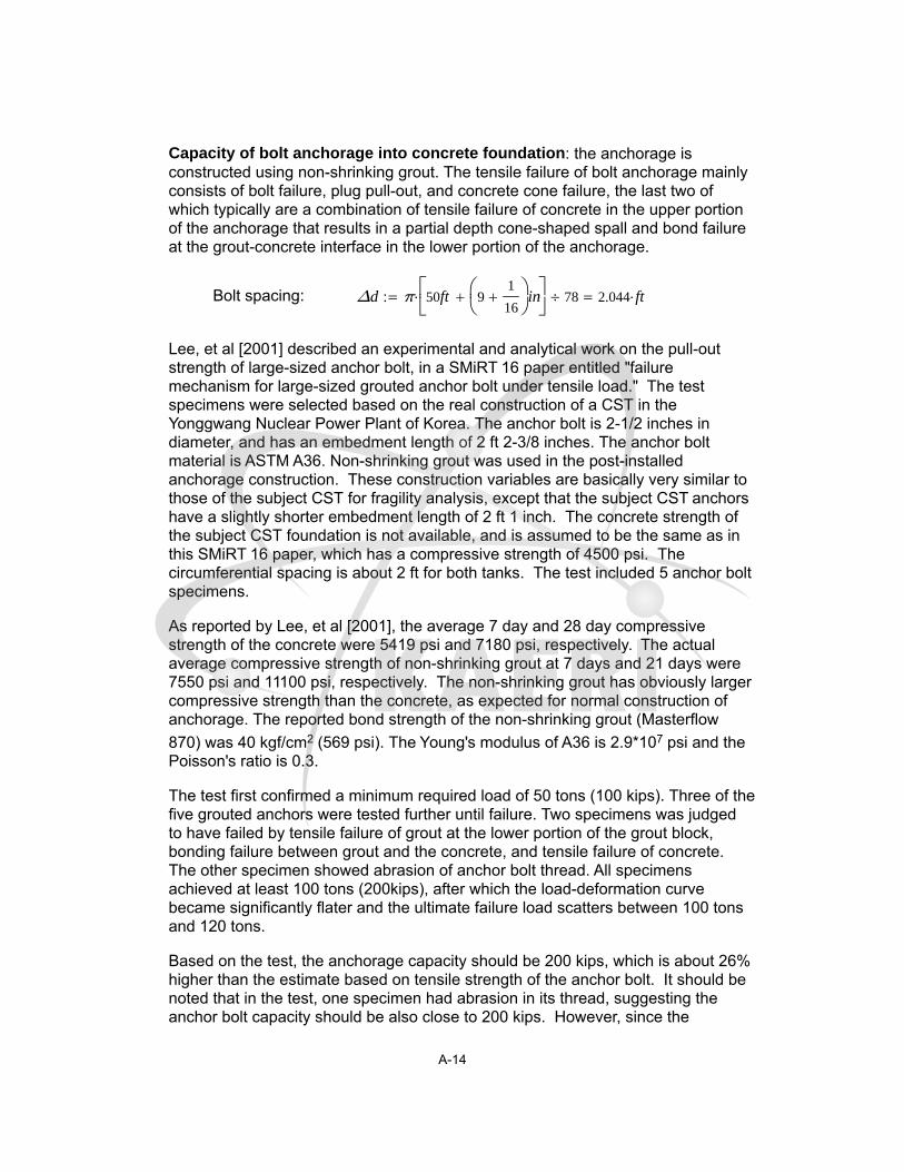
Capacity of bolt anchorage into concrete foundation: the anchorage isconstructed using non-shrinking grout. The tensile failure of bolt anchorage mainlyconsists of bolt failure, plug pull-out, and concrete cone failure, the last two ofwhich typically are a combination of tensile failure of concrete in the upper portionof the anchorage that results in a partial depth cone-shaped spall and bond failureat the grout-concrete interface in the lower portion of the anchorage.

Bolt spacing: Δd π 50ft 91

16

in

78 2.044 ft

Lee, et al [2001] described an experimental and analytical work on the pull-outstrength of large-sized anchor bolt, in a SMiRT 16 paper entitled "failuremechanism for large-sized grouted anchor bolt under tensile load." The testspecimens were selected based on the real construction of a CST in theYonggwang Nuclear Power Plant of Korea. The anchor bolt is 2-1/2 inches indiameter, and has an embedment length of 2 ft 2-3/8 inches. The anchor boltmaterial is ASTM A36. Non-shrinking grout was used in the post-installedanchorage construction. These construction variables are basically very similar tothose of the subject CST for fragility analysis, except that the subject CST anchorshave a slightly shorter embedment length of 2 ft 1 inch. The concrete strength ofthe subject CST foundation is not available, and is assumed to be the same as inthis SMiRT 16 paper, which has a compressive strength of 4500 psi. Thecircumferential spacing is about 2 ft for both tanks. The test included 5 anchor boltspecimens.

As reported by Lee, et al [2001], the average 7 day and 28 day compressivestrength of the concrete were 5419 psi and 7180 psi, respectively. The actualaverage compressive strength of non-shrinking grout at 7 days and 21 days were7550 psi and 11100 psi, respectively. The non-shrinking grout has obviously largercompressive strength than the concrete, as expected for normal construction ofanchorage. The reported bond strength of the non-shrinking grout (Masterflow

870) was 40 kgf/cm2 (569 psi). The Young's modulus of A36 is 2.9*107 psi and thePoisson's ratio is 0.3.

The test first confirmed a minimum required load of 50 tons (100 kips). Three of thefive grouted anchors were tested further until failure. Two specimens was judgedto have failed by tensile failure of grout at the lower portion of the grout block,bonding failure between grout and the concrete, and tensile failure of concrete.The other specimen showed abrasion of anchor bolt thread. All specimensachieved at least 100 tons (200kips), after which the load-deformation curvebecame significantly flater and the ultimate failure load scatters between 100 tonsand 120 tons.

Based on the test, the anchorage capacity should be 200 kips, which is about 26%higher than the estimate based on tensile strength of the anchor bolt. It should benoted that in the test, one specimen had abrasion in its thread, suggesting theanchor bolt capacity should be also close to 200 kips. However, since the

A-14

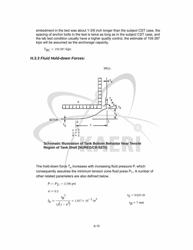
embedment in the test was about 1-3/8 inch longer than the subject CST case, thespacing of anchor bolts in the test is twice as long as in the subject CST case, andthe lab test condition usually have a higher quality control, the estimate of 159.387kips will be assumed as the anchorage capacity.

TBC 159.387 kips

H.3.3 Fluid Hold-down Forces:

Schematic Illustration of Tank Bottom Behavior Near TensileRegion of Tank Shell [NUREG/CR-5270]

The hold-down force Te increases with increasing fluid pressure P, which

consequently assumes the minimum tension zone fluid press PT-. A number of

other related parameters are also defined below.

P PT- 3.196 psi

ν 0.3tS 0.625 in

Ib

tB3

12 1 ν2 1.917 10

3 in3

tB 7 mm

A-15

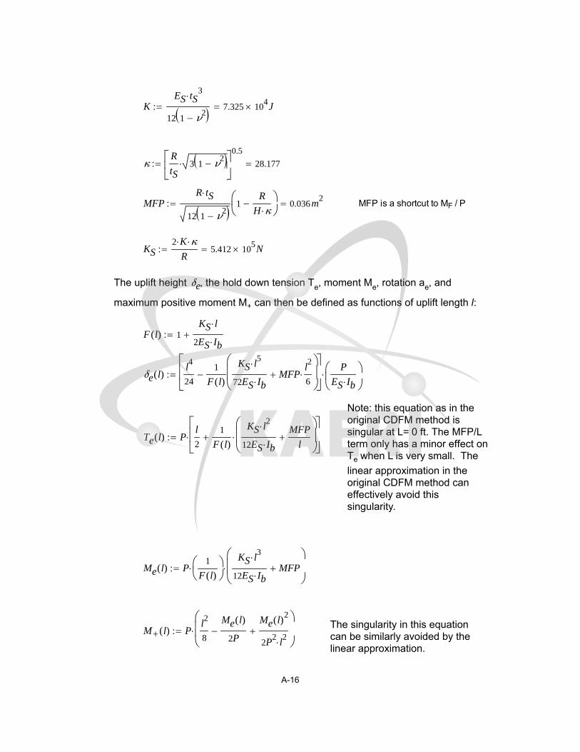
KES tS

3

12 1 ν2 7.325 10

4 J

κR

tS3 1 ν

2

0.5

28.177

MFPR tS

12 1 ν2

1R

H κ

0.036m2 MFP is a shortcut to MF / P

KS2 K κ

R5.412 10

5 N

The uplift height δe, the hold down tension Te, moment Me, rotation ae, and

maximum positive moment M+ can then be defined as functions of uplift length l:

F l( ) 1KS l

2ES Ib

δe l( )l4

24

1

F l( )

KS l5

72ES IbMFP

l2

6

P

ES Ib

Note: this equation as in theoriginal CDFM method issingular at L= 0 ft. The MFP/Lterm only has a minor effect onTe when L is very small. The

linear approximation in theoriginal CDFM method caneffectively avoid thissingularity.

Te l( ) Pl

2

1

F l( )

KS l2

12ES IbMFP

l

Me l( ) P1

F l( )

KS l

3

12ES IbMFP

The singularity in this equationcan be similarly avoided by thelinear approximation.

M+ l( ) Pl2

8

Me l( )

2P

Me l( )2

2P2

l2

A-16

αe l( )P l

312ES Ib

Me l( ) l

2ES Ib

Given

l 0in

l2

24

1

F l( )

KS l3

72ES IbMFP

1

6

0=

lmin Find l( ) 7.65 in

Given

lmax 10in

δe lmax( ) 0.165in=

lmax Find lmax( ) 21.207 in

l lmin lmin 0.1in lmax

Linear Approximation:

i 0lmax lmin( )

0.1in

l_veci lmin i 0.1 in

Te0

Te1

lineδe l_vec( )

in

Te l_vec( )in

lbf

23.391

160.234

Te0 if PT- 0psi Te0 0 lbf

in23.391

lbf

in

Te1 if PT- 0psi Te1 0 lbf

in2

160.234lbf

in2

A-17

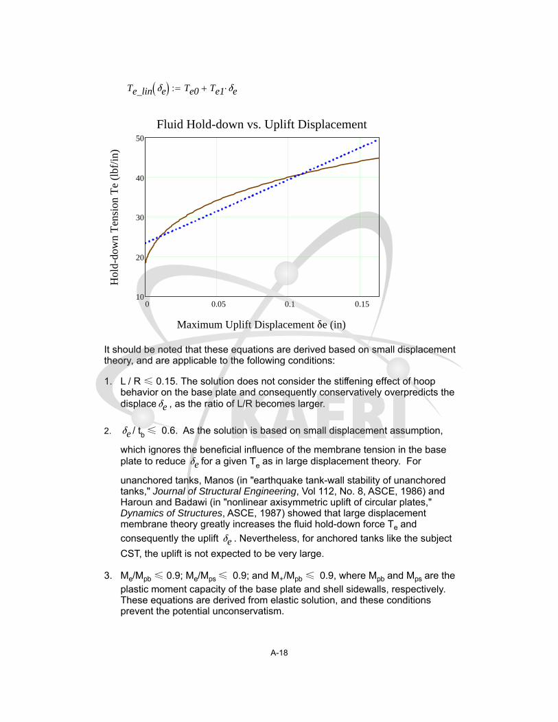
Te_lin δe Te0 Te1 δe

0 0.05 0.1 0.1510

20

30

40

50

Fluid Hold-down vs. Uplift Displacement

Maximum Uplift Displacement δe (in)

Hol

d-do

wn

Ten

sion

Te

(lbf

/in)

It should be noted that these equations are derived based on small displacementtheory, and are applicable to the following conditions:

L / R ≤ 0.15. The solution does not consider the stiffening effect of hoop1.behavior on the base plate and consequently conservatively overpredicts thedisplaceδe , as the ratio of L/R becomes larger.

δe / tb ≤ 0.6. As the solution is based on small displacement assumption,2.

which ignores the beneficial influence of the membrane tension in the baseplate to reduce δe for a given Te as in large displacement theory. For

unanchored tanks, Manos (in "earthquake tank-wall stability of unanchoredtanks," Journal of Structural Engineering, Vol 112, No. 8, ASCE, 1986) andHaroun and Badawi (in "nonlinear axisymmetric uplift of circular plates,"Dynamics of Structures, ASCE, 1987) showed that large displacementmembrane theory greatly increases the fluid hold-down force Te and

consequently the uplift δe . Nevertheless, for anchored tanks like the subject

CST, the uplift is not expected to be very large.

Me/Mpb ≤ 0.9; Me/Mps ≤ 0.9; and M+/Mpb ≤ 0.9, where Mpb and Mps are the3.plastic moment capacity of the base plate and shell sidewalls, respectively.These equations are derived from elastic solution, and these conditionsprevent the potential unconservatism.

A-18

0.6tB 0.165 in

The second requirement leads to maximum δe of 0.165 in, beyond which the small

displacement theory becomes increasingly conservative. The original CDFM solvedthe problem by making a linear approximation of the δe-Te curve in a range of δe =

0 to 0.6tB, and then use the linear equation to extrapolate beyond the 0.6tB topartially account for membrane tension effects. This approach will also be used inthis study.

Te Te_lin

Assessment of the upper limit on the fluid hold-down force: based on a yieldstress σy of 30 ksi, and an ultimate stress of 75 ksi, the fully plastic moment

capacity Mpb of the 7 mm base plate is estimated to be 0.949 kips-inch/inch when

the outer fiber reaches 75 ksi. It is also assumed that the effective hoopcompressive yield stress σye is equal to 45 ksi. The upper limit of the horizontal

component of the membrane tension FH can be found to be:

σye 45 ksi

Mpb

tB3

12

tB

2

75 ksi 0.949kips in

in

FH

σye tS

2κ

Mpb κ

R 0.588

kips

in

4MpbPT- 0.5110.169

lbf

in

FH

2Mpb0.31

1

in

Thus, the upper limit of the fluid hold-down force is estimated to be:

Tm δe 168.841lbf

in1

0.31 δe

in

0.5

The maximum δe can be found by equating Te and Tm:

Given

A-19

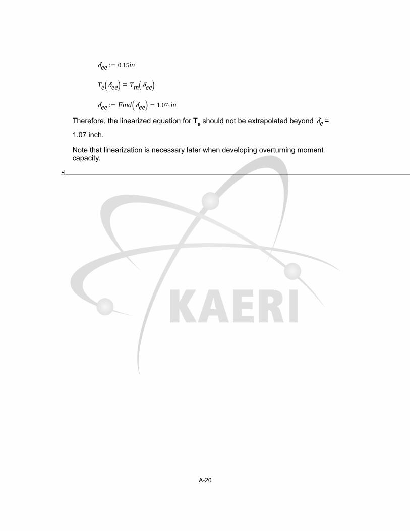
δee 0.15in

Te δee Tm δee =

δee Find δee 1.07 in

Therefore, the linearized equation for Te should not be extrapolated beyond δe =

1.07 inch.

Note that linearization is necessary later when developing overturning momentcapacity.

A-20

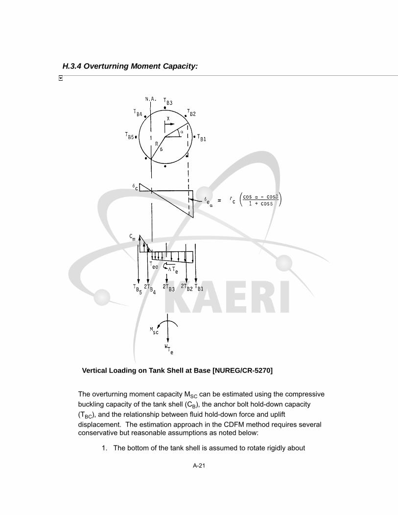
H.3.4 Overturning Moment Capacity:

Vertical Loading on Tank Shell at Base [NUREG/CR-5270]

The overturning moment capacity MSC can be estimated using the compressive

buckling capacity of the tank shell (CB), the anchor bolt hold-down capacity

(TBC), and the relationship between fluid hold-down force and uplift

displacement. The estimation approach in the CDFM method requires severalconservative but reasonable assumptions as noted below:

The bottom of the tank shell is assumed to rotate rigidly about1.

A-21

the neutral axis (plane sections remain plane).

The cross-section of the tank at the top of the top plate of the2.bolt chairs (hc above the base) is assumed to remain

horizontal so that all vertical tank distortions needed to resultin base uplift and mobilization of the anchor bolts must beaccommodated over the height hc.

The compressive stress varies linearly from zero at the3.neutral axis (α=β as in the figure above) to its maximum valueCm at α=180°, as given by Cm = Estsδc/hc ≤ CB (by

converting eq. H-39), where δc is the maximum compressive

shortening.

Summary of parameters:

Cm 12.064kips

in TBC 159.387 kips

Te0 0.023kips

in Te1 0.16

kips

in2

WTe 176.14 kips AB Abolt AB 4.909 in2

EB 29 103ksi

R 25.026 ft

ts 0.625 in Es ES 29 103 ksi

hc 207mm 8.15 in

ha 2ft 1in 25 in

Using the approach outlined in NUREG/CR-5270 instead of the EPRINP-6041-SL appendix H in the following:

δc

Cm hc

Es ts5.424 10

3 in

KB

δc AB EB

ha hc23.294 kips

ΔTe Te1 δc 8.692 104

kips

in

A-22

δea a b( ) δccos a( ) cos b( )

1 cos b( )

Because the bolt pretension TBP is unreliable after a number of years in service, it

is conservatively assumed to be 0.

TBP 0kips

The neutral axis angle β can be determined iteratively using the followingprocedure.

Bolt locations: i 0 77

αi2π

78i

Tfunc α β( ) c TBP KBcos α( ) cos β( )

1 cos β( )

c TBC c TBCif

c 0 c 0if

C1 β( )1 cos β( )

sin β( ) π β( )cos β( )

C2 β( )sin β( ) cos β( ) π β

1 cos β( )

C3 β( )sin β( ) β cos β( )

sin β( ) π β( )cos β( )

C4 β( )β sin β( ) cos β( )

1 cos β( )

TB α β( ) Tfunc α β( )

Cf'm α β( )

WTe TB α β( )2R

Te0 β

C1 β( ) ΔTe C3 β( )

Equating Cf'm and Cm to determine β:

func α β( ) Cf'm α β( ) Cm

A-23

β root func α β( ) β 0 3.1( )

β 2.29114 β180

π 131.273

C'm Cf'm α β( ) 12.064kips

in Cm 12.064

kips

in

Use C'm and β to find the overturning moment capacity MSC:

MSC C'm C2 β( ) R2 TB α β( ) R cos α( )

Te0 R2 2 sin β( ) ΔTe C4 β( ) R

2

MSC 154055.156 kips ft

TB α β( ) 3.846 103 kips

The largest bolt elongation (at α=0) should be checked to ensure that theanchorage has the capability:

δe0 δea α0 β 0.026 in

Elongation ratio:δe0

ha hc0.08 %

The maximum elongation ratio is much smaller than 1%, which is recommended inthe original CDFM method for the A307 bolt. One percent is also considered to be anappropriate percentage value for the A36 anchor bolt used in the subject CSTconstruction.

The maximum tank shell uplift distortion δe0 = 0.026 in, which is much less than the

limit of 0.165 in for the small displacement theory to be applicable in developing thefluid hold-down capacity.

Because there are 78 anchor bolts (the example tank in the original CDFM methodhad only 8), the case where α=0 lies midway between bolts need not be checked.

The uncertainty in HCLPF buckling capacity of the tank shell due to the uncertainσye can lead to an MSC as low as 119133.414 kips-ft or as high as 192156.702

kips-ft. It should be noted that unlike in the original CDFM method, MSC is sensitive

to the estimate of Cm.

Inelastic energy absorption reduction factor k can be applied to linearly computed

A-24

seismic response to obtain the actual overturning moment capacity. The combinedbolt yielding and tank shell buckling failure mode for overturning moment is not brittleso that k can be less than unity. However, as stated in the original CDFM method, itis difficult to make an appropriate estimate of k for this failure mode. Therefore, it isconservatively assumed to be unity.

k 1.0

SMEM

MSC

k MSHSMEe SMEM 1.14 g

Since SMEM is substantially different from SMEe, the above procedure should be

iterated to obtain the appropriate SME estimate. Since there are more capacitiesthat need to be assessed, the iteration is conducted considering all capacities.

H.3.5 Sliding Capacity:

The base plate of the CST has a slight cone ( with a slope of 1 to 96) so that thefluid will always drain away from the center of the tank. This cone is generallycreated by variable thickness of the oiled sand cushion between the tank bottomplate and its foundation. Therefore, the coefficient of friction between the tankbase and its foundation is reasonably assumed to have a conservative value of 0.7in the original CDFM method. For steel over concrete, the coefficient of friction ismore reasonably set to 0.55, as suggested in BNL 52361 [Bandyopadhyay, et al.,1995]. For this study, the lower coefficient of friction of 0.55 is used.

COF 0.55

The sliding shear capacity can then be calculated as,

VSC COF WTe Pa π R2 TB α β( )

3.856 103 kips

The shear capacity of the bolts should not be considered because (a) there is alarge space between the concrete foundation and the anchor bolt chair, and (b)there is a 1/4" diametric clearance in the hole in the anchor bolt chair.

The sliding capacity with a unit inelastic absorption factor as suggested by theoriginal CDFM method:

A-25

SMEV

VSC

k VSHSMEe SMEV 0.426 g

By varying SMEe, the HCLPF shear capacity is found to be 0.426g.

Unlike the example tank in the original CDFM method, the capacity of the CSTappears to be governed by the sliding capacity. The sliding capacity considers onlythe friction between the bottom plate and the foundation.

H.3.6 Fluid Pressure Capacity:

The inelastic energy absorption seismic response reduction factor kμ is suggested

to be 0.8 for HCLPF capacity evaluation:

ku 0.8

For the CDFM hoop membrane stress capacity, it is recommended that the ASMEseismic design limit of 2 SM for primary stress should be used, which is 37.5 ksi for

SA240-type 304 stainless steel:

σa 37.5ksi

The pressure capacity, PCA, at the bottom of the tank shell (the CST has a uniform

shell thickness), can be estimated to be:

PCA t( )σa t

R

PCA tS 78.044 psi

The maximum seismic induced hydrodynamic pressures PSM and the hydrostatic

pressure PST at the bottom of the tank shell are:

PSM H( ) 16.039 psi

PST H( ) 16.25 psi

The HCLPF fluid pressure capacity SMEP can be determined as:

SMEp

PCA tS PST H( )

ku PSM H( )SMEe 2.052 g

The HCLPF fluid pressure capacity does not govern. This agrees with seismicexperience that the fluid pressure capacity seldom appears to govern the seismic

A-26

capacity for normal flat bottomed steel tanks with butt-welded side plates.

Summary of SME capacities:

SMEM 1.14 g

SMEV 0.426 g

SMEp 2.052 g

SMEcr min SMEM SMEV SMEp 0.426 g

SMEe 0.426 g

It should be noted that the controlling SME capacity of 0.426 g based on the CDFMmethod is similar to 0.41 g as reported by Choun, et al [2008]. Both capacities areassociated with the sliding failure mode.

H.3.7 Consideration of Other Capacities:

(1) Slosh height for roof damage: note that even with a SMEe = 0.334 g (the initial

guess), the slosh height is about 4.8 ft. With the HCLPF shear capacity of

SMEe=0.426 g, the sloshing height can be about 6.1 ft, which is lower than the

total height of the head (8.7', as approximated in the beginning part of thiscalculation).

hs 6.093 ft SMEe 0.426 g

The increase of sloshing height is not significant as SMEe increases from 0.334 gto 0.555 g. In addition, as pointed out in the original CDFM method, even if roofdamage might be expected, such damage usually does not impair the ability of thetank to contain fluid.

(2) The CST is assumed to sit on rock/very stiff soil; therefore, soil-tankfoundation interaction is not considered.

(3) Piping failure or failure of nozzles may lead to loss of fluid in the tank, andmore importantly, may impair the normal function of the condensation system. Asreported in the original CDFM method, a significant fraction of the cases ofseismic induced loss of tank contents have been due to piping/nozzle failuresbecause of poor detailing. The CDFM method also stated that a SME evaluationof piping/nozzle failure is necessary only when poor seismic detailing is found inthe involved piping attached to the tank. This analysis assumes that the subjectCST is appropriately detailed, i.e. the piping and nozzle directly attached to thetank are properly designed and constructed so that sufficient piping flexibility can

A-27

be achieved to accommodate large relative seismic anchor movements.

(4) The influence of the building in between the two CSTs on the SME isassessed in the following. The gap between the auxiliary building and the CSTsat the roof level is filled with elastomeric sealant.

The maximum tank shell uplift distortion is found to be 0.026 in, whichcorresponds to a neutral axis angle β of 2.29161 rad. Since the horizontal plane atthe anchor bolt chair is assumed to remain plane and all distortion is assumed tooccur below this level, the rotation angle around the neutral axis can be estimatedto be:

δe0 0.026 in

Rotationδe0

R 1 cos β( )( )5.307 10

5

β 2.291 cos β( ) 0.66

The maximum horizontal displacement at the roof of the auxiliary building, whichis at an elevation of 114' 9" (Parapet elevation, compared to the tank floorelevation of 101' 9"), can be estimated to be:

Rotation 13 ft 8.279 103 in

This horizontal displacement is much less than the width of the seismic separationjoint at the roof elevation, which is 3 in. Therefore, the influence of the auxiliarybuilding to the two CSTs is considered minimal.

The Fragility of CST

SMEHCLPF SMEe 0.426 g

It should be emphasized that the HCLPF SME capacity assumes the RegulatoryGuide 1.60 spectra anchored to the HCLPF SME PGA.

To determine the seismic fragility of the CST, one needs to convert the HCLPFSME PGA to median SME PGA. This conversion requires the estimate of bothaleatory and epistemic uncertainties (βR and βU). The Fragility Method, also

presented along with the original CDFM method, estimates the aleatory andepistemic uncertainties to be 0.2 and 0.27, respectively. These uncertainties arenearly identical to those reported by Choun, et al [2008]. The SME median SMEm

can then be estimated as well.

βR 0.2

A-28

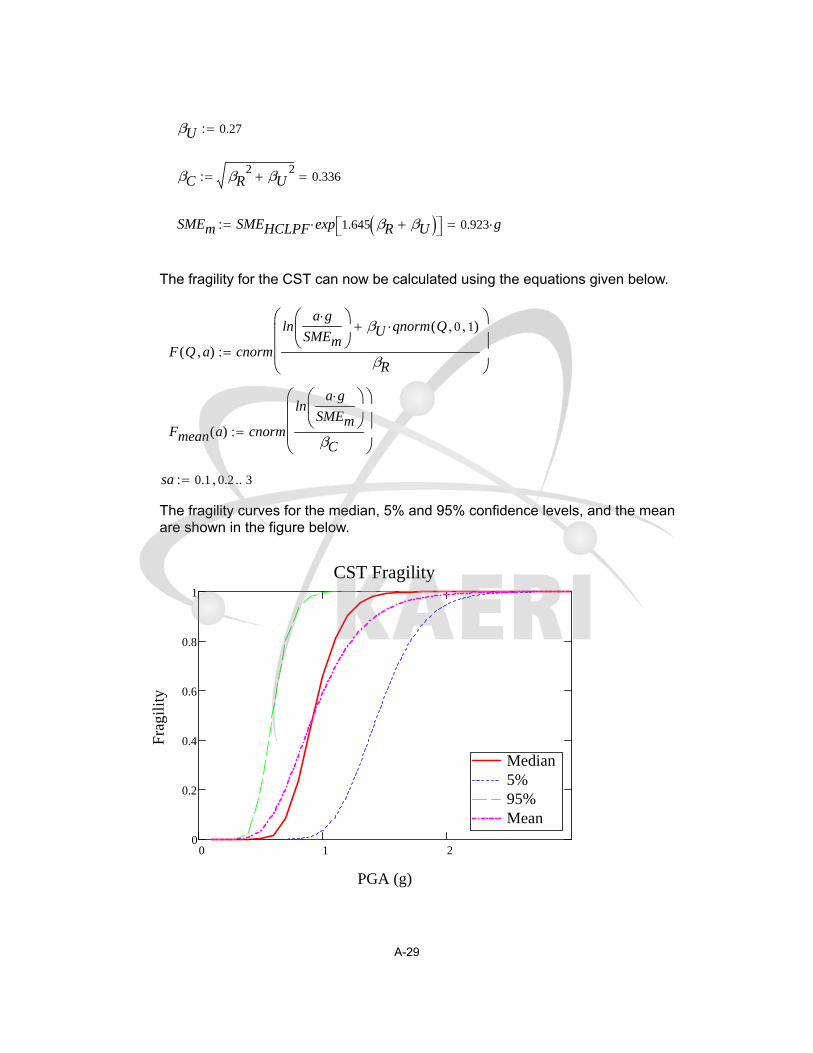
βU 0.27

βC βR2

βU2 0.336

SMEm SMEHCLPF exp 1.645 βR βU 0.923 g

The fragility for the CST can now be calculated using the equations given below.

F Q a( ) cnorm

lna g

SMEm

βU qnorm Q 0 1( )

βR

Fmean a( ) cnorm

lna g

SMEm

βC

sa 0.1 0.2 3

The fragility curves for the median, 5% and 95% confidence levels, and the meanare shown in the figure below.

0 1 20

0.2

0.4

0.6

0.8

1

Median5%95%Mean

CST Fragility

PGA (g)

Fra

gili

ty

A-29

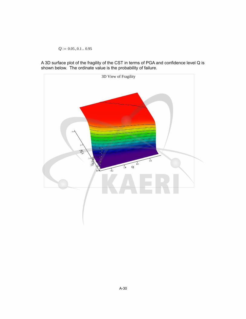
Q 0.05 0.1 0.95

A 3D surface plot of the fragility of the CST in terms of PGA and confidence level Q isshown below. The ordinate value is the probability of failure.

3D View of Fragility

A-30

Appendix B FRAGILITY ANALYSIS OF THE CST WITH DEGRADED STAINLESS TANK SHELL

KAERI Year 3 Task

Fragility Analysis of Condensate Storage Tank

- Degradation Case (A) Stainless Steel Shell Degradation

This calculation is based on the base case CDFM fragility analysis of the subjectCST tank.

The thickness of the tank is reduced for strength calculation, but not for the weightand frequency calculation. The assumption is that the degradation occurs locally atthe base.

For each thickness representing a degradation stage, SMEe must be determined

manually because Mathcad does not support nested solve blocks (using the givenkeyword). Therefore, the calculated SMEe will be saved in a vector.

SCC crack rate was determined using the mechanochemical model for stresscorrosion cracking (SCC) [Nie, et al, 2009, Saito and Kuniya, 2001]. See Section 4.1.1of this report for more details.

year 3600s 24 365

scc_rate 7.494103 in

year

years 60 year

tshell_degraded5

8in scc_rate years 0.175 in

H.1 Introduction

KAERI indicated that the seismic DBE in Korea follows the NRC Reg. Guide 1.60design spectrum shape but with a PGA level scaled down to 0.2 g. An initial HCLPFcapcity was assumed to be 1.67 times of 0.2 g. However, since the Mathcad sheetsin this appendix solve the various equations iteratively by manually setting SMEe to

different values, the following SMEe value of 0.091 g represents the converged

solution for the degradation level of the stainless steel tank shell at 60 years.

SMEe 0.091g

B-1

H.2 Response Evaluation

Section H.2 of this appendix is the same as Section H.2 of Appendix A.

H.3 Capacity Assessment

The seismic overturning moment capacity of the CST at its base, MSC, depends

on the axial compressive buckling capacity of the tank shell Cm, the tensile

hold-down capacity of the anchor bolts including their anchorage and attachmentto the tank TBC, and the hold-down capacity of the fluid pressure acting on the

tank base plate Te.

Although unlikely for larger radius tanks, the tank SME capacity is sometimesgoverned by the sliding shear capacity at the tank base, VSC. Even though it does

not appear that any butt welded steel tank has ever failed due to seismic inducedmembrane hoop stresses due to combined hydrostatic and hydrodynamic fluidpressures, the SME capacity of this failure mode, PCA, should also be checked.

Additional assessment of the seismic capacity may include the possibility andconsequence of the fluid sloshing against the tank roof, foundation failure for soilsites, and possibility of failure of piping or their attachment to the tank.

H.3.1 Compressive Buckling Capacity of the Tank Shell:

The most likely buckling for tanks is the "elephant-foot" buckling near the base ofthe tank shell. The "elephant-foot" buckling is a combined effect of hoop tension,axial (vertical) compression, and restriction of radial deformation of the tank shellby the base plate. "Elephant-foot" buckling does not necessarily lead to failure of atank (e.g., leakage). However, there is no simple capability evaluation method thatcan predict tank performance after the development of "elephant-foot" buckling.Therefore, for a CDFM SME capacity of tanks, the onset of "elephant-foot"buckling will be judged to represent the limit to the compressive buckling capacityof the tank shell. The onset of "elephant-foot" buckling can be estimated usingelastic-plastic collapse theory as presented in the following:

The sidewall thickness near the shell base: ts tshell_degraded 0.175 in

The tank internal pressure near its base: P PC+ 1.313 105 Pa

Elastic modulus of the tank: ES 2.9 104 ksi

The CST shell is made of SA 204-type 304 stainless steel. This material does nothave a flat yield plateau and as strain increases its stress can grow to a minimumultimate stress capacity of 75 ksi. In the CDFM method, an effective yield stress σye

is set to 2.4SM or 45 ksi, in line with the ASME seismic design limit for primary local

membrane plus primary bending [ASME 1983, "ASME Boiler & Pressure Vessel

B-2

Code"]. The potential uncertainty range for σye is reported to be between 30 ksi

and 60 ksi, according to the original CDFM method description.

σye 45ksi

R

ts1.713 10

3

S1R

ts400 4.281

The "elephant-foot" buckling axial stress of the tank shell can be accuratelypredicted to be:

σp

0.6ES

R ts1

P Rσye ts

2

11

1.12 S11.5

S1

σye

36ksi

S1 1

4.548 ksi

The compressive buckling capacity for HCLPF capacity computation utilizes arecommended 0.9 reduction factor of the buckling stress:

Cm 0.9σp ts 0.718kips

in

Buckling capacity of the supported cylindrical shells under combined axial bendingand internal pressure should also be checked although it is unlikely to govern foroverall seismic response of fluid containing tanks. The axial bending inducedbuckling stress, σCB, for such a load case can be conservatively estimated(essentially lower bound) as follows.

A parameter Δγ to be used in the following procedure as an increase factor forinternal pressure can be obtained from Figure 6 of "Buckling of Thin-walledCircular Cylinders," [NASA SP-8007]. Δγ depends on the minimum compressionzone pressure at the base of the tank shell, PC-, corresponding to the time ofmaximum moment.

Considering the potential range on σye of 30 to 60 ksi, the resultant range on σp is16.572 ksi to 26.702 ksi. Consequently, Cm has a range of 9.322 kips/in to 15.02kips/in.

Since Δγ is to be evaluated based on Figure 6 of NASA SP-8007, this figure isdigitized and defined by the following two vectors, in log scale:

B-3

fig6x

1.8197

1.5124

1.395

1.264

1.1422

1.0519

0.94817

0.81296

0.67999

0.52011

0.40087

0.28846

0.18951

0.09283

0.00063874

0.12966

0.22407

0.3071

0.45083

0.57204

0.67305

0.78519

0.86144

0.94893

1.0004

fig6y

1.6448

1.3884

1.3056

1.2088

1.1297

1.0676

1.0058

0.93763

0.86938

0.8017

0.76514

0.7391

0.71278

0.68996

0.66704

0.64849

0.62918

0.62739

0.61269

0.60816

0.60321

0.60915

0.61434

0.6162

0.62796

B-4

Figure 6 of NASA SP-8007: Increase in Axial-CompressiveBuckling-Stress Coefficient of Cylinders due to Internal Pressure

2 1 0 12

1

0

1

log(P/E(R/t_s)^2)

log(

Δγ

)

10linterp fig6x fig6y log 0.166( )( )

0.12004

ipxPC-

ES

R

ts

2

1.679PC-

ES

R

tS

2

0.132

Δγ 10linterp fig6x fig6y log ipx( )( )

0.235

ϕ1

16

R

ts 2.586

γ 1 0.73 1 eϕ 0.325

Note: there is not experimental data for R/t>1500. R

ts1.713 10

3

σCB 0.6γ Δγ( )ES

R ts7.279 ksi

0.9σp 4.094 ksi

σCB exceeds 0.9sp, so it does not govern.

B-5

H.3.2 Bolt Hold-down Capacity:

The bolt hold-down capacity should be determined as the smallest of the bolttensile capacity, anchorage of bolt into concrete foundation, capacity of the topplate of bolt chairs to transfer bolt loads to the vertical chair gussets, attachment ofthe top plate and vertical chair gussets to the tank shell, and the capacity of tankshell to withstand concentrated loads imposed on it by the bolt chairs.

Anchor bolt capacity: the anchor bolt has a diameter of 2 1/2" and is made of A36steel. The tensile capacity can be determined as:

dbolt 2.5in

Abolt

π dbolt2

44.909 in

2

Based on the AISC Code [9th edition, 1989] for threaded A36 bolts:

TBC 1.7Abolt 19.1 ksi 159.387 kips TBC 79.693 tonf

Note that TBC is the capacity of one bolt and the capacity of the interacting

multi-bolts will be considered later.

Anchor bolt chair capacity check: according to the drawing, the anchor boltchairs form a circumferentially continuous construction. Based on the continuouschair construction and the sizing of the plates and weld, it is judged that the anchorbolt chair and its attachment to the tank shell is adequate to transfer the boltcapacity load for the CST tank. The tank shell is also considered to be adequatein withstanding the concentrated loads imposed on it by bolt chairs, especiallybecause the "elephant-foot" buckling capacity is also checked.

tchair 13

8

in 1.375 in

Weld width is 15 mm (5/8") according to the drawing.

Capacity of bolt anchorage into concrete foundation: the anchorage isconstructed using non-shrinking grout. The tensile failure of bolt anchorage mainlyconsists of bolt failure, plug pull-out, and concrete cone failure, the last two ofwhich typically are a combination of tensile failure of concrete in the upper portionof the anchorage that results in a partial depth cone-shaped spall and bond failureat the grout-concrete interface in the lower portion of the anchorage.

Bolt spacing: Δd π 50ft 91

16

in

78 2.044 ft

Lee, et al [2001] described an experimental and analytical work on the pull-outstrength of large-sized anchor bolt, in a SMiRT 16 paper entitled "failuremechanism for large-sized grouted anchor bolt under tensile load." The test

B-6

specimens were selected based on the real construction of a CST in theYonggwang Nuclear Power Plant of Korea. The anchor bolt is 2-1/2 inches indiameter, and has an embedment length of 2 ft 2-3/8 inches. The anchor boltmaterial is ASTM A36. Non-shrinking grout was used in the post-installedanchorage construction. These construction variables are basically very similar tothose of the subject CST for fragility analysis, except that the subject CST anchorshave a slightly shorter embedment length of 2 ft 1 inch. The concrete strength ofthe subject CST foundation is not available, and is assumed to be the same as inthis SMiRT 16 paper, which has a compressive strength of 4500 psi. Thecircumferential spacing is about 2 ft for both tanks. The test included 5 anchor boltspecimens.

As reported by Lee, et al [2001], the average 7 day and 28 day compressivestrength of the concrete were 5419 psi and 7180 psi, respectively. The actualaverage compressive strength of non-shrinking grout at 7 days and 21 days were7550 psi and 11100 psi, respectively. The non-shrinking grout has obviously largercompressive strength than the concrete, as expected for normal construction ofanchorage. The reported bond strength of the non-shrinking grout (Masterflow

870) was 40 kgf/cm2 (569 psi). The Young's modulus of A36 is 2.9*107 psi and thePoisson's ratio is 0.3.

The test first confirmed a minimum required load of 50 tons (100 kips). Three of thefive grouted anchors were tested further until failure. Two specimens was judgedto have failed by tensile failure of grout at the lower portion of the grout block,bonding failure between grout and the concrete, and tensile failure of concrete.The other specimen showed abrasion of anchor bolt thread. All specimensachieved at least 100 tons (200kips), after which the load-deformation curvebecame significantly flater and the ultimate failure load scatters between 100 tonsand 120 tons.

Based on the test, the anchorage capacity should be 200 kips, which is about 26%higher than the estimate based on tensile strength of the anchor bolt. It should benoted that in the test, one specimen had abrasion in its thread, suggesting theanchor bolt capacity should be also close to 200 kips. However, since theembedment in the test was about 1-3/8 inch longer than the subject CST case, thespacing of anchor bolts in the test is twice as long as in the subject CST case, andthe lab test condition usually have a higher quality control, the estimate of 159.387kips will be assumed as the anchorage capacity.

TBC 159.387 kips

B-7

H.3.3 Fluid Hold-down Forces:

Schematic Illustration of Tank Bottom Behavior NearTensile Region of Tank Shell [NUREG/CR-5270]

The hold-down force Te increases with increasing fluid pressure P, which

consequently assumes the minimum tension zone fluid press PT-. A number of

other related parameters are also defined below.

P PT- 13.461 psi

ν 0.3tS 0.625 in

Ib

tB3

12 1 ν2 1.917 10

3 in3

ts 0.175 in

tB 7 mmK

ES ts3

12 1 ν2 1.618 10

3 J

κR

ts3 1 ν

2

0.5

53.194

MFPR ts

12 1 ν2

1R

H κ

0.01m2 MFP is a shortcut to MF / P

B-8

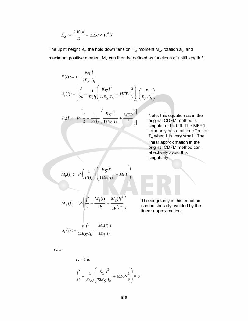
KS2 K κ

R2.257 10

4 N

The uplift height δe, the hold down tension Te, moment Me, rotation ae, and

maximum positive moment M+ can then be defined as functions of uplift length l:

F l( ) 1KS l

2ES Ib

δe l( )l4

24

1

F l( )

KS l5

72ES IbMFP

l2

6

P

ES Ib

Note: this equation as in theoriginal CDFM method issingular at L= 0 ft. The MFP/Lterm only has a minor effect onTe when L is very small. The

linear approximation in theoriginal CDFM method caneffectively avoid thissingularity.

Te l( ) Pl

2

1

F l( )

KS l2

12ES IbMFP

l

Me l( ) P1

F l( )

KS l

3

12ES IbMFP

The singularity in this equationcan be similarly avoided by thelinear approximation.

M+ l( ) Pl2

8

Me l( )

2P

Me l( )2

2P2

l2

αe l( )P l

312ES Ib

Me l( ) l

2ES Ib

Given

l 0 in

l2

24

1

F l( )

KS l3

72ES IbMFP

1

6

0=

B-9

lmin Find l( ) 7.516 in

Given

lmax 10in

δe lmax( ) 0.165in=

lmax Find lmax( ) 13.278 in

l lmin lmin 0.1in lmax

Linear Approximation:

i 0lmax lmin( )

0.1in

l_veci lmin i 0.1 in

Te0

Te1

lineδe l_vec( )

in

Te l_vec( )in

lbf

79.594

211.542

Te0 if PT- 0psi Te0 0 lbf

in79.594

lbf

in

Te1 if PT- 0psi Te1 0 lbf

in2

211.542lbf

in2

Te_lin δe Te0 Te1 δe

B-10

0 0.05 0.1 0.150

50

100

150

Fluid Hold-down vs Uplift Displacement

Maximum Uplift Displacement δe (in)

Hol

d-do

wn

Ten

sion

Te

(lbf

/in)

It should be noted that these equations are derived based on small displacementtheory, and are applicable to the following conditions:

L / R ≤ 0.15. The solution does not consider the stiffening effect of hoop1.behavior on the base plate and consequently conservatively overpredicts thedisplaceδe , as the ratio of L/R becomes larger.

δe / tb≤ 0.6. As the solution is based on small displacement assumption,2.

which ignores the beneficial influence of the membrane tension in the baseplate to reduce δe for a given Te as in large displacement theory. For

unanchored tanks, Manos (in "earthquake tank-wall stability of unanchoredtanks," Journal of Structural Engineering, Vol 112, No. 8, ASCE, 1986) andHaroun and Badawi (in "nonlinear axisymmetric uplift of circular plates,"Dynamics of Structures, ASCE, 1987) showed that large displacementmembrane theory greatly increases the fluid hold-down force Te and

consequently the uplift δe . Nevertheless, for anchored tanks like the subject

CST, the uplift is not expected to be very large.

Me/Mpb ≤ 0.9; Me/Mps≤ 0.9; and M+/Mpb ≤ 0.9, where Mpb and Mps are the3.plastic moment capacity of the base plate and shell sidewalls, respectively.These equations are derived from elastic solution, and these conditionsprevent the potential unconservatism.

0.6tB 0.165 in

B-11

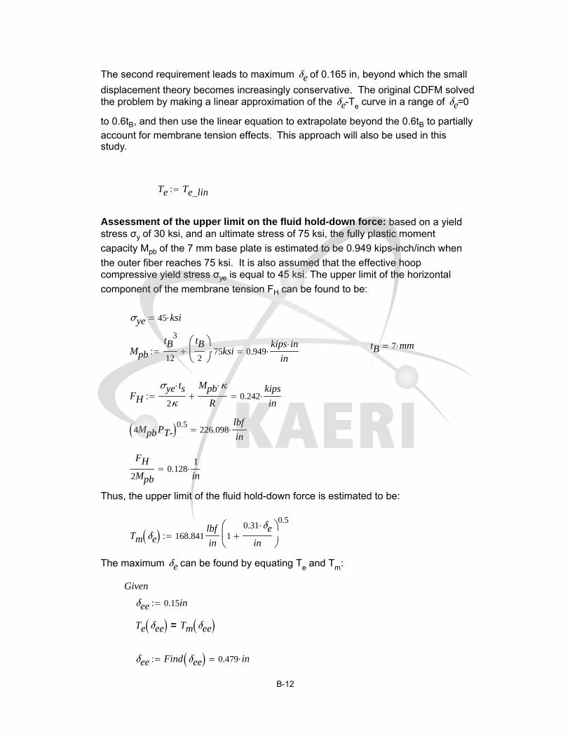
The second requirement leads to maximum δe of 0.165 in, beyond which the small

displacement theory becomes increasingly conservative. The original CDFM solvedthe problem by making a linear approximation of the δe-Te curve in a range of δe=0

to 0.6tB, and then use the linear equation to extrapolate beyond the 0.6tB to partiallyaccount for membrane tension effects. This approach will also be used in thisstudy.

Te Te_lin

Assessment of the upper limit on the fluid hold-down force: based on a yieldstress σy of 30 ksi, and an ultimate stress of 75 ksi, the fully plastic moment

capacity Mpb of the 7 mm base plate is estimated to be 0.949 kips-inch/inch when

the outer fiber reaches 75 ksi. It is also assumed that the effective hoopcompressive yield stress σye is equal to 45 ksi. The upper limit of the horizontal

component of the membrane tension FH can be found to be:

σye 45 ksi

tB 7 mmMpb

tB3

12

tB

2

75 ksi 0.949kips in

in

FH

σye ts

2κ

Mpb κ

R 0.242

kips

in

4MpbPT- 0.5226.098

lbf

in

FH

2Mpb0.128

1

in

Thus, the upper limit of the fluid hold-down force is estimated to be:

Tm δe 168.841lbf

in1

0.31 δe

in

0.5

The maximum δe can be found by equating Te and Tm:

Given

δee 0.15in

Te δee Tm δee =

δee Find δee 0.479 in

B-12

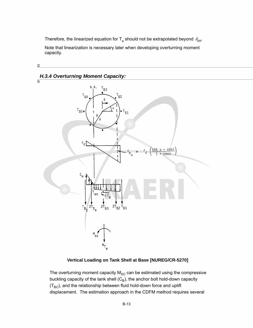
Therefore, the linearized equation for Te should not be extrapolated beyond δee.

Note that linearization is necessary later when developing overturning momentcapacity.

H.3.4 Overturning Moment Capacity:

Vertical Loading on Tank Shell at Base [NUREG/CR-5270]

The overturning moment capacity MSC can be estimated using the compressive

buckling capacity of the tank shell (CB), the anchor bolt hold-down capacity

(TBC), and the relationship between fluid hold-down force and uplift

displacement. The estimation approach in the CDFM method requires several

B-13

conservative but reasonable assumptions as noted below:

The bottom of the tank shell is assumed to rotate rigidly about the1.neutral axis (plane sections remain plane).

The cross-section of the tank at the top of the top plate of the bolt2.chairs (hc above the base) is assumed to remain horizontal so that all

vertical tank distortions needed to result in base uplift andmobilization of the anchor bolts must be accommodated over theheight hc.

The compressive stress varies linearly from zero at the neutral axis3.(α=β as in the figure above) to its maximum value Cm at α=180°, as

given by Cm = Estsδc/hc ≤ CB (by converting eq. H-39), where δc is

the maximum compressive shortening.

Summary of parameters:

Cm 0.718kips

in TBC 159.387 kips

Te0 0.08kips

in Te1 0.212

kips

in2

WTe 204.591 kips AB Abolt AB 4.909 in2

EB 29 103ksi

R 25.026 ft

ts 0.175 in Es ES 29 103 ksi

hc 207mm 8.15 in

ha 2ft 1in 25 in

Using the approach outlined in NUREG/CR-5270 instead of the EPRINP-6041-SL appendix H in the following:

δc

Cm hc

Es ts1.15 10

3 in

KB

δc AB EB

ha hc4.94 kips

ΔTe Te1 δc 2.434 104

kips

in

B-14

δea a b( ) δccos a( ) cos b( )

1 cos b( )

Because the bolt pretension TBP is unreliable after a number of years in service, it

is conservatively assumed to be 0.TBP 0kips

The neutral axis angle β can be determined iteratively using the followingprocedure.

Bolt locations: i 0 77

αi2π

78i

Tfunc α β( ) c TBP KBcos α( ) cos β( )

1 cos β( )

c TBC c TBCif

c 0 c 0if

C1 β( )1 cos β( )

sin β( ) π β( )cos β( )

C2 β( )sin β( ) cos β( ) π β

1 cos β( )

C3 β( )sin β( ) β cos β( )

sin β( ) π β( )cos β( )

C4 β( )β sin β( ) cos β( )

1 cos β( )

TB α β( ) Tfunc α β( )

Cf'm α β( )

WTe TB α β( )2R

Te0 β

C1 β( ) ΔTe C3 β( )

Equating Cf'm and Cm to determine β:

func α β( ) Cf'm α β( ) Cm

β root func α β( ) β 0 3.14159( )

β 1.61646 β180

π 92.617

B-15

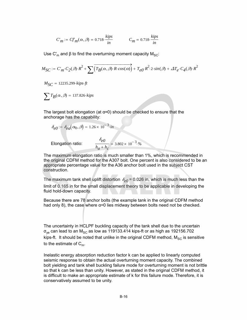
C'm Cf'm α β( ) 0.718kips

in Cm 0.718

kips

in

Use C'm and β to find the overturning moment capacity MSC:

MSC C'm C2 β( ) R2 TB α β( ) R cos α( )

Te0 R2 2 sin β( ) ΔTe C4 β( ) R

2

MSC 12235.299 kips ft

TB α β( ) 137.826 kips

The largest bolt elongation (at α=0) should be checked to ensure that theanchorage has the capability:

δe0 δea α0 β 1.26 103 in

Elongation ratio:δe0

ha hc3.802 10

3 %

The maximum elongation ratio is much smaller than 1%, which is recommended inthe original CDFM method for the A307 bolt. One percent is also considered to be anappropriate percentage value for the A36 anchor bolt used in the subject CSTconstruction.

The maximum tank shell uplift distortion δe0 = 0.026 in, which is much less than the

limit of 0.165 in for the small displacement theory to be applicable in developing thefluid hold-down capacity.

Because there are 78 anchor bolts (the example tank in the original CDFM methodhad only 8), the case where α=0 lies midway between bolts need not be checked.

The uncertainty in HCLPF buckling capacity of the tank shell due to the uncertainσye can lead to an MSC as low as 119133.414 kips-ft or as high as 192156.702

kips-ft. It should be noted that unlike in the original CDFM method, MSC is sensitive

to the estimate of Cm.

Inelastic energy absorption reduction factor k can be applied to linearly computedseismic response to obtain the actual overturning moment capacity. The combinedbolt yielding and tank shell buckling failure mode for overturning moment is not brittleso that k can be less than unity. However, as stated in the original CDFM method, itis difficult to make an appropriate estimate of k for this failure mode. Therefore, it isconservatively assumed to be unity.

B-16

k 1.0

SMEM

MSC

k MSHSMEe SMEM 0.091 g

Since SMEM is substantially different from SMEe, the above procedure should be

iterated to obtain the appropriate SME estiamte. The resultant SMEe is found to be

0.97g.

H.3.5 Sliding Capacity:

The base plate of the CST has a slight cone ( with a slope of 1 to 96) so that thefluid will always drain away from the center of the tank. This cone is generallycreated by variable thickness of the oiled sand cushion between the tank bottomplate and its foundation. Therefore, the coefficient of friction between the tankbase and its foundation is reasonably assumed to have a conservative value of0.55:

COF 0.55

The sliding shear capacity can then be calculated as,

VSC COF WTe Pa π R2 TB α β( )

2.531 103 kips

The shear capacity of the bolts should not be considered because (a) there is alarge space between the concrete foundation and the anchor bolt chair, and (b)there is a 1/4" diametric clearance in the hole in the anchor bolt chair.

The sliding capacity with a unit inelastic absorption factor as suggested by theoriginal CDFM method:

SMEV

VSC

k VSHSMEe SMEV 0.279 g

Unlike the example tank in the original CDFM method, the capacity of the CSTappears to be governed by the sliding capacity. The sliding capacity considers onlythe friction between the bottom plate and the foundation.

B-17

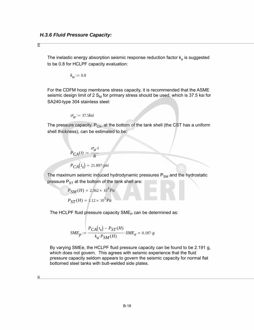
H.3.6 Fluid Pressure Capacity:

The inelastic energy absorption seismic response reduction factor kμ is suggested

to be 0.8 for HCLPF capacity evaluation:

ku 0.8

For the CDFM hoop membrane stress capacity, it is recommended that the ASMEseismic design limit of 2 SM for primary stress should be used, which is 37.5 ksi for

SA240-type 304 stainless steel:

σa 37.5ksi

The pressure capacity, PCA, at the bottom of the tank shell (the CST has a uniform

shell thickness), can be estimated to be:

PCA t( )σa t

R

PCA ts 21.897 psi

The maximum seismic induced hydrodynamic pressures PSM and the hydrostatic

pressure PST at the bottom of the tank shell are:

PSM H( ) 2.362 104 Pa

PST H( ) 1.12 105 Pa

The HCLPF fluid pressure capacity SMEP can be determined as:

SMEp

PCA ts PST H( )

ku PSM H( )SMEe 0.187 g

By varying SMEe, the HCLPF fluid pressure capacity can be found to be 2.191 g,which does not govern. This agrees with seismic experience that the fluidpressure capacity seldom appears to govern the seismic capacity for normal flatbottomed steel tanks with butt-welded side plates.

B-18

Summary of SME capacities:

SMEM 0.091 g

SMEV 0.279 g

SMEp 0.187 g

SMEcr min SMEM SMEV SMEp 0.091 g

SMEe 0.091 g

if SMEcr SMEM= "Moment" if SMEcr SMEV= "Shear" "Fluid Pressure" "Moment"

ts 0.175 in

Summary of results:

Years: 0 5 10 15 20 25 30 35 40ts (in): 0.625 0.591 0.557 0.523 0.489 0.455 0.421 0.387 0.353SME: 0.426 0.409 0.393 0.376 0.360 0.343 0.326 0.310 0.294SMEM: 1.14 1.047 0.953 0.858 0.762 0.667 0.571 0.476 0.383SMEV: 0.426 0.409 0.393 0.376 0.360 0.343 0.326 0.310 0.294SMEP: 2.052 1.896 1.741 1.586 1.430 1.275 1.120 0.964 0.809Mode: Shear Shear Shear Shear Shear Shear Shear Shear Shear

Years: 45 50 55 60 65 70 75 80ts (in): 0.319 0.285 0.251 0.217 0.184 0.150SME: 0.278 0.218 0.152 0.091 NASMEM: 0.290 0.218 0.152 0.091 NASMEV: 0.278 0.276 0.277 0.28 NASMEP: 0.654 0.498 0.343 0.187 NAMode: Shear MomentMomentMoment NA

H.3.7 Consideration of Other Capacities:

(1) Slosh height for roof damage: note that even with a SMEe = 0.334 g (the initial

guess), the slosh height is about 4.8 ft. With the HCLPF shear capacity of

SMEe=0.555 g, the sloshing height can be about 7.9 ft, which is close to the total

height of the head (8.7', as approximated in the beginning part of this calculation).

hs 1.302 ft SMEe 0.091 g

The increase of sloshing height is not significant as SMEe increases from 0.334 gto 0.555 g. In addition, as pointed out in the original CDFM method, even if roofdamage might be expected, such damage usually does not impair the ability of thetank to contain fluid.

(2) The CST is assumed to sit on rock/very stiff soil; therefore, soil-tankfoundation interaction is not considered.

B-19

(3) Piping failure or failure of nozzles may lead to loss of fluid in the tank, andmore importantly, may impair the normal function of the condensation system. Asreported in the original CDFM method, a significant fraction of the cases ofseismic induced loss of tank contents have been due to piping/nozzle failuresbecause of poor detailing. The CDFM method also stated that a SME evaluationof piping/nozzle failure is only necessary when poor seismic detailing is found inthe involved piping attached to the tank. This analysis assumes that the subjectCST is appropriately detailed, i.e. the piping and nozzle directly attached to thetank are properly designed and constructed so that sufficient piping flexibility canbe achieved to accommodate large relative seismic anchor movements.

(4) The influence of the building in between the two CSTs on the SME areassessed in the following. The gap between the auxiliary building and the CSTsat the roof level is filled with elastomeric sealant.

The maximum tank shell uplift distortion is found to be 0.026 in, whichcorresponds to a neutral axis angle β of 2.29161 rad. Since the horizontal plane atthe anchor bolt chair is assumed to remain plane and all distortion is assumed tooccur below this level, the rotation angle around the neutral axis can be estimatedto be:

Rotationδe0

R 1 cos β( )( )4.014 10

6

β 1.616 cos β( ) 0.046

The maximum horizontal displacement at the roof of the auxiliary building, whichis at an elevation of 114' 9" (Parapet elevation, compared to the tank floorelevation of 101' 9"), can be estimated to be:

Rotation 13 ft 0.000626 in

This horizontal displacement is much less than the width of the seismic separationjoint at the roof elevation, which is 3 in. Therefore, the influence of the auxiliarybuilding to the two CSTs is considered minimal.

The Fragility of CST Based on Degraded Conditions

Summary of results:

Years: 0 5 10 15 20 25 30 35 40ts (in): 0.625 0.591 0.557 0.523 0.489 0.455 0.421 0.387 0.353SME: 0.426 0.409 0.393 0.376 0.360 0.343 0.326 0.310 0.294SMEM: 1.14 1.047 0.953 0.858 0.762 0.667 0.571 0.476 0.383SMEV: 0.426 0.409 0.393 0.376 0.360 0.343 0.326 0.310 0.294SMEP: 2.052 1.896 1.741 1.586 1.430 1.275 1.120 0.964 0.809Mode: Shear Shear Shear Shear Shear Shear Shear Shear Shear

Years: 45 50 55 60 65 70 75 80ts (in): 0.319 0.285 0.251 0.217 0.184 0.150

B-20

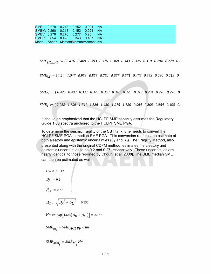
( )SME: 0.278 0.218 0.152 0.091 NASMEM: 0.290 0.218 0.152 0.091 NASMEV: 0.278 0.276 0.277 0.28 NASMEP: 0.654 0.498 0.343 0.187 NAMode: Shear MomentMomentMoment NA

SMEHCLPF 0.426 0.409 0.393 0.376 0.360 0.343 0.326 0.310 0.294 0.278 0.2(

SMEM 1.14 1.047 0.953 0.858 0.762 0.667 0.571 0.476 0.383 0.290 0.218 0.1(

SMEV 0.426 0.409 0.393 0.376 0.360 0.343 0.326 0.310 0.294 0.278 0.276 0.(

SMEP 2.052 1.896 1.741 1.586 1.430 1.275 1.120 0.964 0.809 0.654 0.498 0.(

It should be emphasized that the HCLPF SME capacity assumes the RegulatoryGuide 1.60 spectra anchored to the HCLPF SME PGA.

To determine the seismic fragility of the CST tank, one needs to convert theHCLPF SME PGA to median SME PGA. This conversion requires the estimate ofboth aleatory and epistemic uncertainties (βR and βU). The Fragility Method, also

presented along with the original CDFM method, estimates the aleatory andepistemic uncertainties to be 0.2 and 0.27, respectively. These uncertainties arenearly identical to those reported by Choun, et al [2008]. The SME median SMEm

can then be estimated as well.

i 0 1 12

βR 0.2

βU 0.27

βC βR2

βU2 0.336

Hm exp 1.645 βR βU 2.167

SMEmiSMEHCLPFi

Hm

SMEMmiSMEMi

Hm

B-21

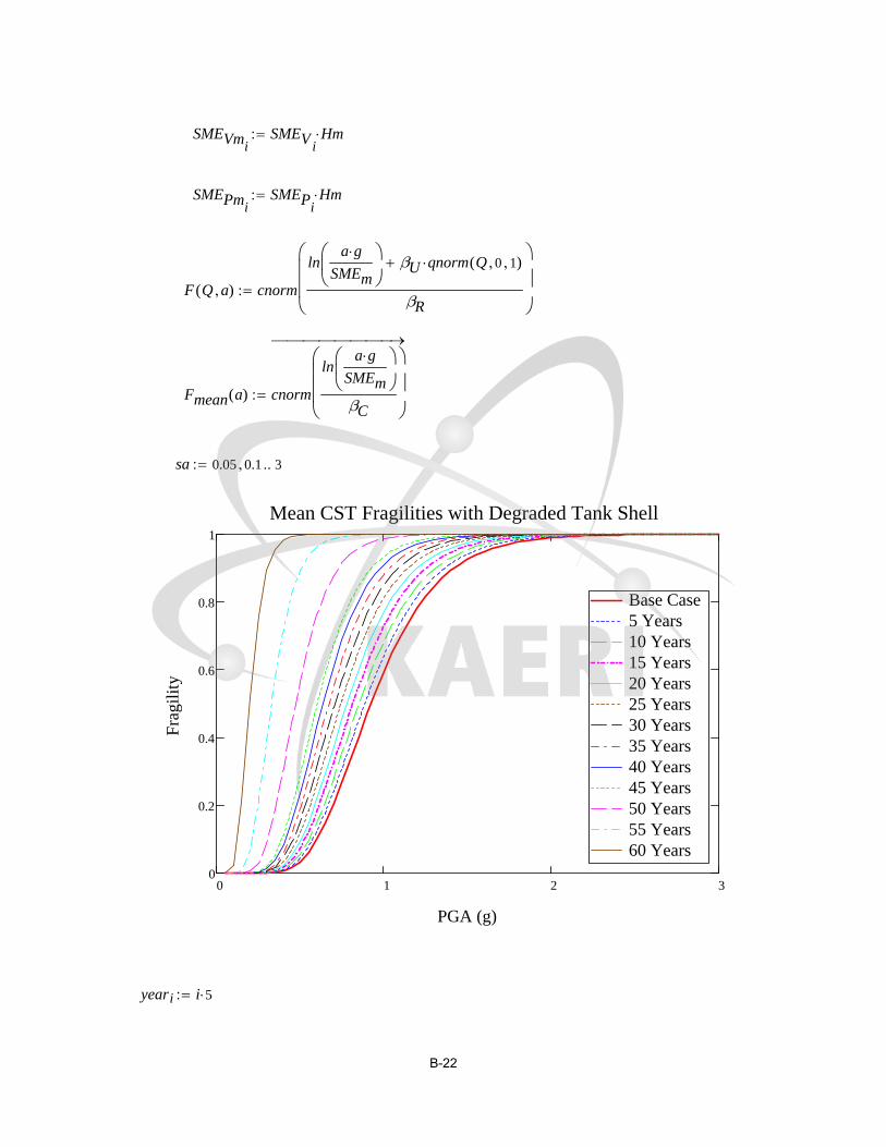
SMEVmiSMEVi

Hm

SMEPmiSMEPi

Hm

F Q a( ) cnorm

lna g

SMEm

βU qnorm Q 0 1( )

βR

Fmean a( ) cnorm

lna g

SMEm

βC

sa 0.05 0.1 3

0 1 2 30

0.2

0.4

0.6

0.8

1

Base Case5 Years10 Years15 Years20 Years25 Years30 Years35 Years40 Years45 Years50 Years55 Years60 Years

Mean CST Fragilities with Degraded Tank Shell

PGA (g)

Fra

gili

ty

yeari i 5

B-22

0 5 10 15 20 25 30 35 40 45 50 55 600

0.5

1

1.5

2

2.5

HCLPF CapacityOverturning Moment CapacitySliding CapacityFluid Pressure Capacity

Time (year)

HC

LP

F F

ragi

lity

Cap

acit

y (g

)

B-23

0 5 10 15 20 25 30 35 40 45 50 55 600

1

2

3

4

5

Median CapacityOverturning Moment CapacitySliding CapacityFluid Pressure Capacity

Time (year)

Med

ian

Fra

gili

ty C

apac

ity

(g)

B-24

218 0.152 0.091 )T

g

152 0.091 )T

g

.277 0.28 )T

g

343 0.187 )T

g

B-25

Appendix C FRAGILITY ANALYSIS OF THE CST WITH DEGRADED ANCHOR BOLTS

KAERI Year 3 Task

Fragility Analysis of Condensate Storage Tank

- Degradation Case (B) A36 Anchor Bolt

The power model for steel corrosion was chosen for modeling the degradation of the anchor bolts,from the Year 2 annual report [Nie, et al, 2009]. Parameters C and α are identified based on"Performance of weathering steel in bridges," by Albrecht and Naeemi [1984].

For severity consideration, it is conservatively assumed that the Ulchin NPP units 3 & 4 areexposed to a marine condition.

C 70.6

α 0.79

X t( ) C tα μm

y 0 5 80

X y( )

0-39.912·10

0.017

0.024

0.03

0.035

0.041

0.046

0.051

...

in

C-1

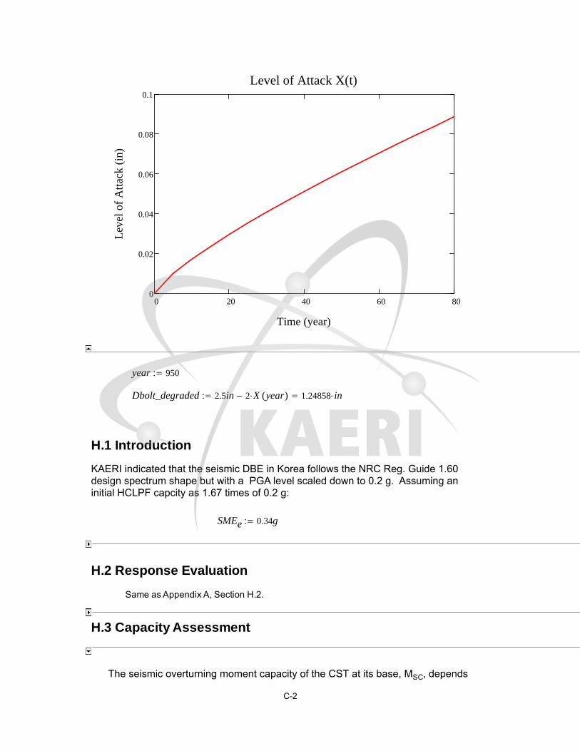
0 20 40 60 800

0.02

0.04

0.06

0.08

0.1

Level of Attack X(t)

Time (year)

Lev

el o

f A

ttac

k (i

n)

year 950

Dbolt_degraded 2.5in 2 X year( ) 1.24858 in

H.1 Introduction

KAERI indicated that the seismic DBE in Korea follows the NRC Reg. Guide 1.60design spectrum shape but with a PGA level scaled down to 0.2 g. Assuming aninitial HCLPF capcity as 1.67 times of 0.2 g:

SMEe 0.34g

H.2 Response Evaluation

Same as Appendix A, Section H.2.

H.3 Capacity Assessment

The seismic overturning moment capacity of the CST at its base, MSC, depends

C-2

on the axial compressive buckling capacity of the tank shell Cm, the tensile

hold-down capacity of the anchor bolts including their anchorage and attachmentto the tank TBC, and the hold-down capacity of the fluid pressure acting on the

tank base plate Te.

Although unlikely for larger radius tanks, the tank SME capacity is sometimesgoverned by the sliding shear capacity at the tank base, VSC. Even though it does

not appear that any butt welded steel tank has ever failed due to seismic inducedmembrane hoop stresses due to combined hydrostatic and hydrodynamic fluidpressures, the SME capacity of this failure mode, PCA, should also be checked.

Additional assessment of the seismic capacity may include the possibility andconsequence of the fluid sloshing against the tank roof, foundation failure for soilsites, and possibility of failure of piping or their attachment to the tank.

H.3.1 Compressive Buckling Capacity of the Tank Shell:

The most likely buckling for tanks is the "elephant-foot" buckling near the base ofthe tank shell. The "elephant-foot" buckling is a combined effect of hoop tension,axial (vertical) compression, and restriction of radial deformation of the tank shellby the base plate. "Elephant-foot" buckling does not necessarily lead to failure of atank (e.g., leakage). However, there is no simple capacility evaluation method thatcan predict tank performance after the development of "elephant-foot" buckling.Therefore, for a CDFM SME capacity of tanks, the onset of "elephant-foot"buckling will be judged to represent the limit to the compressive buckling capacityof the tank shell. The onset of "elephant-foot" buckling can be estimated usingelastic-plastic collapse theory as presented in the following:

The sidewall thickness near the shell base: ts tS 0.625 in

The tank internal pressure near its base: P PC+ 1.839 105 Pa

Elastic modulus of the tank: ES 2.9 104 ksi

The CST shell is made of SA 204-type 304 stainless steel. This material does nothave a flat yield plateau and as strain increases its stress can grow to a minimumultimate stress capacity of 75 ksi. In the CDFM method, an effective yield stress σye

is set to 2.4SM or 45 ksi, in line with the ASME seismic design limit for primary local

membrane plus primary bending [ASME 1983, "ASME Boiler & Pressure VesselCode"]. The potential uncertainty range for σye is reported to be between 30 ksi

and 60 ksi, according to the original CDFM method description.

σye 45ksi

C-3

R

ts480.5

S1R

ts400 1.201

The "elephant-foot" buckling axial stress of the tank shell can be accuratelypredicted to be:

σp

0.6ES

R ts1

P Rσye ts

2

11

1.12 S11.5

S1

σye

36ksi

S1 1

21.847 ksi

The compressive buckling capacity for HCLPF capacity computation utilizes arecommended 0.9 reduction factor of the buckling stress:

Cm 0.9σp ts 12.289kips

in

Buckling capacity of the supported cylindrical shells under combined axial bendingand internal pressure should also be checked although it is unlikely to govern foroverall seismic response of fluid containing tanks. The axial bending inducedbuckling stress, σCB, for such a load case can be conservatively estimated(essentially lower bound) as follows.

A parameter Δγ to be used in the following procedure as an increase factor forinternal pressure can be obtained from Figure 6 of "Buckling of Thin-walledCircular Cylinders," [NASA SP-8007]. Δγ depends on the minimum compressionzone pressure at the base of the tank shell, PC-, corresponding to the time ofmaximum moment.

Considering the potential range on σye of 30 to 60 ksi, the resultant range on σp is16.572 ksi to 26.702 ksi. Consequently, Cm has a range of 9.322 kips/in to 15.02kips/in.

PC-

ES

R

tS

2

0.14

From Figure 6 of NASA SP-8007: Δγ 0.12

ϕ1

16

R

ts 1.37

γ 1 0.73 1 eϕ 0.455

C-4

σCB 0.6γ Δγ( )ES

R ts23.737 ksi

0.9σp 19.663 ksi

σCB exceeds 0.9sp, so it does not govern.

H.3.2 Bolt Hold-down Capacity:

The bolt hold-down capacity should be determined as the smallest of the bolttensile capacity, anchorage of bolt into concrete foundation, capacity of the topplate of bolt chairs to transfer bolt loads to the vertical chair gussets, attachment ofthe top plate and vertical chair gussets to the tank shell, and the capacity of tankshell to withstand concentrated loads imposed on it by bolt chairs.

Anchor bolt capacity: the anchor bolt has a diameter of 2 1/2" and is made of A36steel. The tensile capacity can be determined as:

dbolt Dbolt_degraded 1.249 in

Abolt

π dbolt2

41.224 in

2

Based on the AISC Code [9th edition, 1989] for threaded A36 bolts:

TBC 1.7Abolt 19.1 ksi 39.756 kips TBC 19.878 tonf

Note that TBC is the capacity of one bolt and the capacity of the interacting

multi-bolts will be considered later.

Anchor bolt chair capacity check: according to the drawing, the anchor boltchairs form a circumferentially continuous construction. Based on the continuouschair construction and the sizing of the plates and weld, it is judged that the anchorbolt chair and its attachment to the tank shell is adequate to transfer the boltcapacity load for the CST. The tank shell is also considered to be adequate inwithstanding the concentrated loads imposed on it by bolt chairs, especiallybecause the "elephant-foot" buckling capacity is also checked.

tchair 13

8

in 1.375 in

Weld width is 15 mm (5/8") according to the drawing.

Capacity of bolt anchorage into concrete foundation: the anchorage isconstructed using non-shrinking grout. The tensile failure of bolt anchorage mainlyconsists of bolt failure, plug pull-out, and concrete cone failure, the last two of

C-5

which typically are a combination of tensile failure of concrete in the upper portionof the anchorage that results in a partial depth cone-shaped spall and bond failureat the grout-concrete interface in the lower portion of the anchorage.

Bolt spacing: Δd π 50ft 91

16

in

78 2.044 ft

Lee, et al [2001] described an experimental and analytical work on the pull-outstrength of large-sized anchor bolt, in a SMiRT 16 paper entitled "failuremechanism for large-sized grouted anchor bolt under tensile load." The testspecimens were selected based on the real construction of CST in the YonggwangNuclear Power Plant of Korea. The anchor bolt is 2-1/2 inches in diameter, andhas an embedment length of 2 ft 2-3/8 inches. The anchor bolt material is ASTMA36. Non-shrinking grout was used in the post-installed anchorage construction.These construction variables are basically very similar to those of the subject CSTfor fragility analysis, except that the subject CST anchors have a slightly shorterembedment length of 2 ft 1 inch. The concrete strength of the subject CSTfoundation is not available, and is assumed to be the same as in this SMiRT 16paper, which has a compressive strength of 4500 psi. The circumferential spacingis about 2 ft for both tanks. The test included 5 anchor bolt specimens.

As reported by Lee, et al [2001], the average 7 day and 28 day compressivestrength of the concrete were 5419 psi and 7180 psi, respectively. The actualaverage compressive strength of non-shrinking grout at 7 days and 21 days were7550 psi and 11100 psi, respectively. The non-shrinking grout has obviously largercompressive strength than the concrete, as expected for normal construction ofanchorage. The reported bond strength of the non-shrinking grout (Masterflow

870) was 40 kgf/cm2 (569 psi). The Young's modulus of A36 is 2.9*107 psi and thePoisson's ratio is 0.3.

The test first confirmed a minimum required load of 50 tons (100 kips). Three of thefive grouted anchors were tested further until failure. Two specimens was judgedto have failed by tensile failure of grout at the lower portion of the grout block,bonding failure between grout and the concrete, and tensile failure of concrete.The other specimen showed abrasion of anchor bolt thread. All specimensachieved at least 100 tons (200kips), after which the load-deformation curvebecame significantly flatter and the ultimate failure load scatters between 100 tonsand 120 tons.

Based on the test, the anchorage capacity should be 200 kips, which is about 26%higher than the estimate based on tensile strength of the anchor bolt. It should benoted that in the test, one specimen had abrasion in its thread, suggesting theanchor bolt capacity should be also close to 200 kips. However, since theembedment in the test was about 1-3/8 inch longer than the subject CST case, thespacing of anchor bolts in the test is twice as long as in the subject CST case, andthe lab test condition usually have a higher quality control, the estimate of 159.387kips will be assumed as the anchorage capacity.

TBC 39.756 kips

C-6

H.3.3 Fluid Hold-down Forces:

Schematic Illustration of Tank Bottom Behavior NearTensile Region of Tank Shell [NUREG/CR-5270]

The hold-down force Te increases with increasing fluid pressure P, which

consequently assumes the minimum tension zone fluid press PT-. A number of

other related parameters are also defined below.

P PT- 5.831 psi

ν 0.3tS 0.625 in

Ib

tB3

12 1 ν2 1.917 10

3 in3

tB 7 mm

KES tS

3

12 1 ν2 7.325 10

4 J

κR

tS3 1 ν

2

0.5

28.177

MFPR tS

12 1 ν2

1R

H κ

0.036m2 MFP is a shortcut to MF / P

C-7

KS2 K κ

R5.412 10

5 N

The uplift height δe, the hold down tension Te, moment Me, rotation ae, and

maximum positive moment M+ can then be defined as functions of uplift length l:

F l( ) 1KS l

2ES Ib

δe l( )l4

24

1

F l( )

KS l5

72ES IbMFP

l2

6

P

ES Ib

Note: this equation as in theoriginal CDFM method issingular at L= 0 ft. The MFP/Lterm only has a minor effectonL / R ≤ 0.15. The solutiondoes not consider thestiffening effect of hoopbehavior on the base plate andconsequently conservativelyoverpredicts the displaceδe ,

as the ratio of L/R becomeslarger. Te when L is verysmall. The linearapproximation in the originalCDFM method can effectivelyavoid this singularity.

Te l( ) Pl

2

1

F l( )

KS l2

12ES IbMFP

l

Me l( ) P1

F l( )

KS l

3

12ES IbMFP

The singularity in this equationcan be similarly avoided by thelinear approximation.

M+ l( ) Pl2

8

Me l( )

2P

Me l( )2

2P2

l2

αe l( )P l

312ES Ib

Me l( ) l

2ES Ib

Given

l 0in

l2

24

1

F l( )

KS l3

72ES IbMFP

1

6

0=

C-8

lmin Find l( ) 7.65 in

Given

lmax 10in

δe lmax( ) 0.165in=

lmax Find lmax( ) 18.34 in

l lmin lmin 0.1in lmax

Linear Approximation:

i 0lmax lmin( )

0.1in

l_veci lmin i 0.1 in

Te0

Te1

lineδe l_vec( )

in

Te l_vec( )in

lbf

39.846

228.734

Te0 if PT- 0psi Te0 0 lbf

in39.846

lbf

in

Te1 if PT- 0psi Te1 0 lbf

in2

228.734lbf

in2

Te_lin δe Te0 Te1 δe

C-9

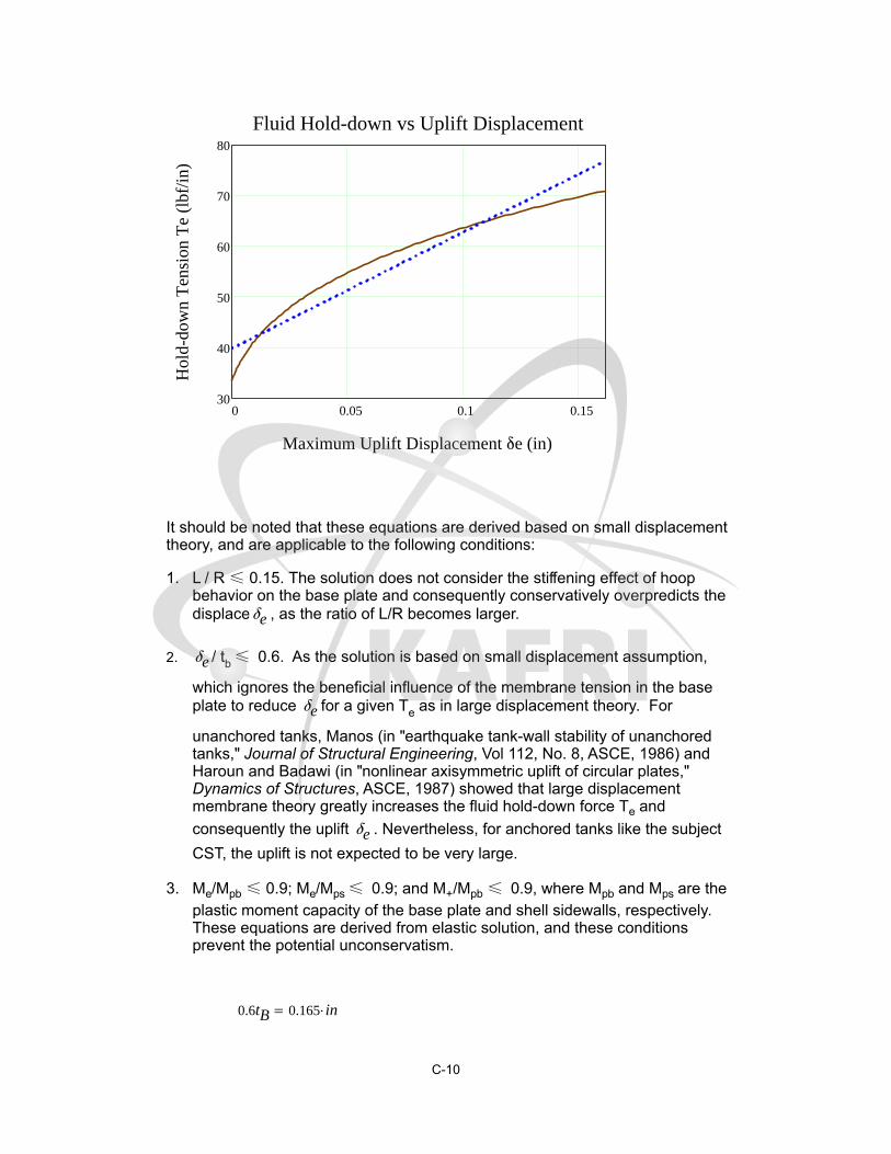
0 0.05 0.1 0.1530

40

50

60

70

80

Fluid Hold-down vs Uplift Displacement

Maximum Uplift Displacement δe (in)

Hol

d-do

wn

Ten

sion

Te

(lbf

/in)

It should be noted that these equations are derived based on small displacementtheory, and are applicable to the following conditions:

L / R ≤ 0.15. The solution does not consider the stiffening effect of hoop1.behavior on the base plate and consequently conservatively overpredicts thedisplaceδe , as the ratio of L/R becomes larger.

δe / tb ≤ 0.6. As the solution is based on small displacement assumption,2.

which ignores the beneficial influence of the membrane tension in the baseplate to reduce δe for a given Te as in large displacement theory. For

unanchored tanks, Manos (in "earthquake tank-wall stability of unanchoredtanks," Journal of Structural Engineering, Vol 112, No. 8, ASCE, 1986) andHaroun and Badawi (in "nonlinear axisymmetric uplift of circular plates,"Dynamics of Structures, ASCE, 1987) showed that large displacementmembrane theory greatly increases the fluid hold-down force Te and

consequently the uplift δe . Nevertheless, for anchored tanks like the subject

CST, the uplift is not expected to be very large.

Me/Mpb ≤ 0.9; Me/Mps ≤ 0.9; and M+/Mpb ≤ 0.9, where Mpb and Mps are the3.plastic moment capacity of the base plate and shell sidewalls, respectively.These equations are derived from elastic solution, and these conditionsprevent the potential unconservatism.

0.6tB 0.165 in

C-10

The second requirement leads to maximum δe of 0.165 in, beyond which the small

displacement theory becomes increasingly conservative. The original CDFM solvedthe problem by making a linear approximation of the δe-Te curve in a range of δe=0

to 0.6tB, and then use the linear equation to extrapolate beyond the 0.6tB to partiallyaccount for membrane tension effects. This approach will also be used in thisstudy.

Te Te_lin

Assessment of the upper limit on the fluid hold-down force: based on a yieldstress σy of 30 ksi, and an ultimate stress of 75 ksi, the fully plastic moment

capacity Mpb of the 7 mm base plate is estimated to be 0.949 kips-inch/inch when

the outer fiber reaches 75 ksi. It is also assumed that the effective hoopcompressive yield stress σye is equal to 45 ksi. The upper limit of the horizontal

component of the membrane tension FH can be found to be:

σye 45 ksi

Mpb

tB3

12

tB

2

75 ksi 0.949kips in

in

FH

σye tS

2κ

Mpb κ

R 0.588

kips

in

4MpbPT- 0.5148.811

lbf

in

FH

2Mpb0.31

1

in

Thus, the upper limit of the fluid hold-down force is estimated to be:

Tm δe 168.841lbf

in1

0.31 δe

in

0.5

The maximum δe can be found by equating Te and Tm:

Given

δee 0.15in

Te δee Tm δee =

δee Find δee 0.633 in

C-11

Therefore, the linearized equation for Te should not be extrapolated beyond δe =

1.805 inch.

Note that linearization is necessary later when developing overturning momentcapacity.

H.3.4 Overturning Moment Capacity:

Vertical Loading on Tank Shell at Base [NUREG/CR-5270]

The overturning moment capacity MSC can be estimated using the compressive

C-12

buckling capacity of the tank shell (CB), the anchor bolt hold-down capacity

(TBC), and the relationship between fluid hold-down force and uplift

displacement. The estimation approach in the CDFM method requires severalconservative but reasonable assumptions as noted below:

The bottom of the tank shell is assumed to rotate rigidly about the1.neutral axis (plane sections remain plane).

The cross-section of the tank at the top of the top plate of the bolt2.chairs (hc above the base) is assumed to remain horizontal so that all

vertical tank distortions needed to result in base uplift andmobilization of the anchor bolts must be accommodated over theheight hc.

The compressive stress varies linearly from zero at the neutral axis3.(α=β as in the figure above) to its maximum value Cm at α=180°, as

given by Cm = Estsδc/hc ≤ CB (by converting eq. H-39), where δc is

the maximum compressive shortening.

Summary of parameters:

Cm 12.289kips

in TBC 39.756 kips

Te0 0.04kips

in Te1 0.229

kips

in2

WTe 183.444 kips AB Abolt AB 1.224 in2

EB 29 103ksi

R 25.026 ft

ts 0.625 in Es ES 29 103 ksi

hc 207mm 8.15 in

ha 2ft 1in 25 in

Using the approach outlined in NUREG/CR-5270 instead of the EPRINP-6041-SL appendix H in the following:

δc

Cm hc

Es ts5.526 10

3 in

KB

δc AB EB

ha hc5.919 kips

C-13

ΔTe Te1 δc 1.264 103

kips

in

δea a b( ) δccos a( ) cos b( )

1 cos b( )

Because the bolt pretension TBP is unreliable after a number of years in service, it

is conservatively assumed to be 0.

TBP 0kips

The neutral axis angle β can be determined iteratively using the followingprocedure.

Bolt locations: i 0 77

αi2π

78i

Tfunc α β( ) c TBP KBcos α( ) cos β( )

1 cos β( )

c TBC c TBCif

c 0 c 0if

C1 β( )1 cos β( )

sin β( ) π β( )cos β( )

C2 β( )sin β( ) cos β( ) π β

1 cos β( )

C3 β( )sin β( ) β cos β( )

sin β( ) π β( )cos β( )

C4 β( )β sin β( ) cos β( )

1 cos β( )

TB α β( ) Tfunc α β( )

Cf'm α β( )

WTe TB α β( )2R

Te0 β

C1 β( ) ΔTe C3 β( )

Equating Cf'm and Cm to determine β:

func α β( ) Cf'm α β( ) Cm

β root func α β( ) β 0 3.1( )

C-14

β 2.65998 β180

π 152.406

C'm Cf'm α β( ) 12.289kips

in Cm 12.289

kips

in

Use C'm and β to find the overturning moment capacity MSC:

MSC C'm C2 β( ) R2 TB α β( ) R cos α( )

Te0 R2 2 sin β( ) ΔTe C4 β( ) R

2

MSC 78565.847 kips ft

TB α β( ) 2.095 103 kips

The largest bolt elongation (at α=0) should be checked to ensure that theanchorage has the capability:

δe0 δea α0 β 0.092 in

Elongation ratio:δe0

ha hc0.276 %

The maximum elongation ratio is much smaller than 1%, which is recommended inthe original CDFM method for the A307 bolt. One percent is also considered to be anappropriate percentage value for the A36 anchor bolt used in the subject CSTconstruction.

The maximum tank shell uplift distortion δe0 = 0.026 in, which is much less than the

limit of 0.165 in for the small displacement theory to be applicable in developing thefluid hold-down capacity.

Because there are 78 anchor bolts (the example tank in the original CDFM methodhad only 8), the case where α=0 lies midway between bolts need not be checked.

The uncertainty in HCLPF buckling capacity of the tank shell due to the uncertainσye can lead to an MSC as low as 119133.414 kips-ft or as high as 192156.702

kips-ft. It should be noted that unlike in the original CDFM method, MSC is sensitive

to the estimate of Cm.

Inelastic energy absorption reduction factor k can be applied to linearly computedseismic response to obtain the actual overturning moment capacity. The combinedbolt yielding and tank shell buckling failure mode for overturning moment is not brittleso that k can be less than unity. However, as stated in the original CDFM method, it

C-15

is difficult to make an appropriate estimate of k for this failure mode. Therefore, it isconservatively assumed to be unity.

k 1.0

SMEM

MSC

k MSHSMEe SMEM 0.582 g

Since SMEM is substantially different from SMEe, the above procedure should be

iterated to obtain the appropriate SME estiamte. The resultant SMEe is found to be

0.97g.

H.3.5 Sliding Capacity:

The base plate of the CST has a slight cone ( with a slope of 1 to 96) so that thefluid will always drain away from the center of the tank. This cone is generallycreated by variable thickness of the oiled sand cushion between the tank bottomplate and its foundation. Therefore, the coefficient of friction between the tankbase and its foundation is reasonably assumed to have a conservative value of0.55:

COF 0.55

The sliding shear capacity can then be calculated as,

VSC COF WTe Pa π R2 TB α β( )

3.076 103 kips

The shear capacity of the bolts should not be considered because (a) there is alarge space between the concrete foundation and the anchor bolt chair, and (b)there is a 1/4" diametric clearance in the hole in the anchor bolt chair.

The sliding capacity with a unit inelastic absorption factor as suggested by theoriginal CDFM method:

SMEV

VSC

k VSHSMEe SMEV 0.339 g

By varying SMEe, the HCLPF shear capacity is found to be 0.555g.

Unlike the example tank in the original CDFM method, the capacity of the CSTappears to be governed by the sliding capacity. The sliding capacity considers onlythe friction between the bottom plate and the foundation.

C-16

H.3.6 Fluid Pressure Capacity:

The inelastic energy absorption seismic response reduction factor kμ is suggested

to be 0.8 for HCLPF capacity evaluation:

ku 0.8

For the CDFM hoop membrane stress capacity, it is recommended that the ASMEseismic design limit of 2 SM for primary stress should beused, which is 37.5 ksi for

SA240-type 304 stainless steel:

σa 37.5ksi

The pressure capacity, PCA, at the bottom of the tank shell (the CST has a uniform

shell thickness), can be estimated to be:

PCA t( )σa t

R

PCA tS 78.044 psi

The maximum seismic induced hydrodynamic pressures PSM and the hydrostatic

pressure PST at the bottom of the tank shell are:

PSM H( ) 8.826 104 Pa

PST H( ) 1.12 105 Pa

The HCLPF fluid pressure capacity SMEP can be determined as:

SMEp

PCA tS PST H( )

ku PSM H( )SMEe 2.052 g

By varying SMEe, the HCLPF fluid pressure capacity can be found to be 2.191 g,which does not govern. This agrees with seismic experience that the fluidpressure capacity seldom appears to govern the seismic capacity for normal flatbottomed steel tanks with butt-welded side plates.

Summary of SME capacities:

SMEM 0.582 g

SMEV 0.339 g

C-17

SMEp 2.052 g

SMEcr min SMEM SMEV SMEp 0.339 g

SMEe 0.34 g

if SMEcr SMEM= "Moment" if SMEcr SMEV= "Shear" "Fluid Pressure" "Shear"

dbolt 1.249 in

Summary of results:

Years: 0 5 10 15 20 25 30 35 40db (in): 2.5 2.48 2.466 2.453 2.441 2.429 2.418 2.408 2.398SME: 0.426 0.425 0.424 0.423 0.423 0.422 0.422 0.422 0.421SMEM: 1.140 1.136 1.132 1.129 1.126 1.123 1.120 1.117 1.115SMEV: 0.426 0.425 0.424 0.423 0.423 0.422 0.422 0.422 0.421SMEP: 2.052 2.052 2.052 2.052 2.052 2.052 2.052 2.052 2.052Mode: Shear Shear Shear Shear Shear Shear Shear Shear Shear

Years: 45 50 55 60 65 70 75 80db (in): 2.323SME: 0.42 0.42 0.419 0.418SMEM: 1.11 1.105 1.100 1.095SMEV: 0.42 0.42 0.419 0.418SMEP: 2.052 2.052 2.052 2.052Mode: Shear Shear Shear Shear Shear Shear Shear Shear

Even with a degradation level of half of bolt diameter, the SME is still as high as0.34 g and shear failure mode still dominates. The overturning moment capacity isabout 0.582 g at this level of degradation (approximate 950 years using the currentpower model) and the fluid pressure capacity remains unchanged as expected.This high level of SME capcity and reliability is believed to be attributed to the largenumber of bolts.

H.3.7 Consideration of Other Capacities:

(1) Slosh height for roof damage: note that even with a SMEe = 0.334 g (the initial

guess), the slosh height is about 4.8 ft. With the HCLPF shear capacity of

SMEe=0.555 g, the sloshing height can be about 7.9 ft, which is close to the total

height of the head (8.7', as approximated in the beginning part of this calculation).

hs 4.863 ft SMEe 0.34 g

The increase of sloshing height is not significant as SMEe increases from 0.334 gto 0.555 g. In addition, as pointed out in the original CDFM method, even if roofdamage might be expected, such damage usually does not impair the ability of thetank to contain fluid.

C-18

(2) The CST is assumed to sit on rock/very stiff soil; therefore, soil-tankfoundation interaction is not considered.

(3) Piping failure or failure of nozzles may lead to loss of fluid in the tank, andmore importantly, may impair the normal function of the condensation system. Asreported in the original CDFM method, a significant fraction of the cases ofseismic induced loss of tank contents have been due to piping/nozzle failuresbecause of poor detailing. The CDFM method also stated that a SME evaluationof piping/nozzle failure is only necessary when poor seismic detailing is found inthe involved piping attached to the tank. This analysis assumes that the subjectCST is appropriately detailed, i.e. the piping and nozzle directly attached to thetank are properly designed and constructed so that sufficient piping flexibility canbe achieved to accommodate large relative seismic anchor movements.

(4) The influence of the building in between the two CSTs on the SME areassessed in the following. The gap between the auxiliary building and the CSTsat the roof level is filled with elastomeric sealant.

The maximum tank shell uplift distortion is found to be 0.026 in, whichcorresponds to a neutral axis angle β of 2.29161 rad. Since the horizontal plane atthe anchor bolt chair is assumed to remain plane and all distortion is assumed tooccur below this level, the rotation angle around the neutral axis can be estimatedto be:

Rotationδe0

R 1 cos β( )( )1.618 10

4

β 2.66 cos β( ) 0.886

The maximum horizontal displacement at the roof of the auxiliary building, whichis at an elevation of 114' 9" (Parapet elevation, compared to the tank floorelevation of 101' 9"), can be estimated to be:

Rotation 13 ft 0.025 in

This horizontal displacement is much less than the width of the seismic separationjoint at the roof elevation, which is 3 in. Therefore, the influence of the auxiliarybuilding to the two CSTs is considered minimal.

The Fragility of CST

Summary of results:

Years: 0 5 10 15 20 25 30 35 40db (in): 2.5 2.48 2.466 2.453 2.441 2.429 2.418 2.408 2.398SME: 0.426 0.425 0.424 0.423 0.423 0.422 0.422 0.422 0.421SMEM: 1.140 1.136 1.132 1.129 1.126 1.123 1.120 1.117 1.115SMEV: 0.426 0.425 0.424 0.423 0.423 0.422 0.422 0.422 0.421SMEP: 2.052 2.052 2.052 2.052 2.052 2.052 2.052 2.052 2.052Mode: Shear Shear Shear Shear Shear Shear Shear Shear Shear

C-19

Years: 45 50 55 60 65 70 75 80db (in): 2.323SME: 0.42 0.42 0.419 0.418SMEM: 1.11 1.105 1.100 1.095SMEV: 0.42 0.42 0.419 0.418SMEP: 2.052 2.052 2.052 2.052Mode: Shear Shear Shear Shear Shear Shear Shear Shear

SMEHCLPF 0.426 0.425 0.424 0.423 0.423 0.422 0.422 0.422 0.421 0.42 0.42 0(

SMEM 1.140 1.136 1.132 1.129 1.126 1.123 1.120 1.117 1.115 1.11 1.105 1.100(

SMEV 0.426 0.425 0.424 0.423 0.423 0.422 0.422 0.422 0.421 0.42 0.42 0.419(

SMEP 2.052 2.052 2.052 2.052 2.052 2.052 2.052 2.052 2.052 2.052 2.052 2.052(

It should be emphasized that the HCLPF SME capacity assumes the RegulatoryGuide 1.60 spectra anchored to the HCLPF SME PGA.

To determine the seismic fragility of the CST, one needs to convert the HCLPFSME PGA to median SME PGA. This conversion requires the estimate of bothaleatory and epistemic uncertainties (βR and βU). The Fragility Method, also

presented along with the original CDFM method, estimates the aleatory andepistemic uncertainties to be 0.2 and 0.27, respectively. These uncertainties arenearly identical to those reported by Choun, et al [2008]. The SME median SMEm

can then be estimated as well.

i 0 1 12

βR 0.2

βU 0.27

βC βR2

βU2 0.336

Hm exp 1.645 βR βU 2.167

SMEmiSMEHCLPFi

Hm

SMEMmiSMEMi

Hm

C-20

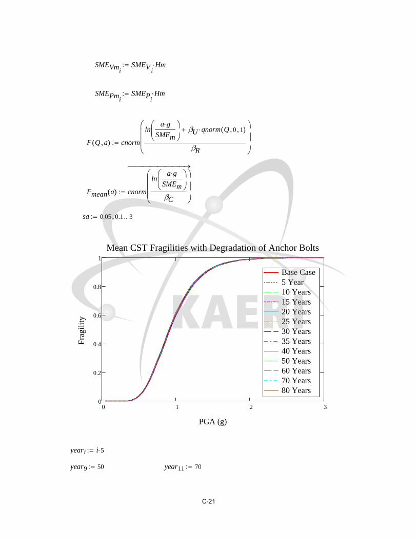
SMEVmiSMEVi

Hm

SMEPmiSMEPi

Hm

F Q a( ) cnorm

lna g

SMEm

βU qnorm Q 0 1( )

βR

Fmean a( ) cnorm

lna g

SMEm

βC

sa 0.05 0.1 3

0 1 2 30

0.2

0.4

0.6

0.8

1

Base Case5 Year10 Years15 Years20 Years25 Years30 Years35 Years40 Years50 Years60 Years70 Years80 Years

Mean CST Fragilities with Degradation of Anchor Bolts

PGA (g)

Fra

gili

ty

yeari i 5

year9 50 year11 70

C-21

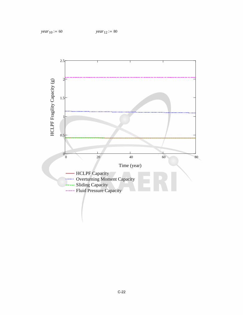
year10 60 year12 80

0 20 40 60 800

0.5

1

1.5

2

2.5

HCLPF CapacityOverturning Moment CapacitySliding CapacityFluid Pressure Capacity

Time (year)

HC

LP

F F

ragi

lity

Cap

acit

y (g

)

C-22

0 20 40 60 800

1

2

3

4

5

Median CapacityOverturning Moment CapacitySliding CapacityFluid Pressure Capacity

Time (year)

Med

ian

Fra

gili

ty C

apac

ity

(g)

C-23

0.419 0.418 )T

g

0 1.095 )T

g

0.418 )T

g

2 2.052 )T

g

C-24

Appendix D FRAGILITY ANALYSIS OF THE CST WITH FOUNDATION CONCRETE CRACKING – APPLICATION OF MODEL C-1

KAERI Year 3 Task

Fragility Analysis of Condensate Storage Tank

- Degradation Case (C-1) Anchorage (concrete)Degradation

This case utilizes the concrete degradation data recorded in Korea NPPs and testdata of dynamic anchorage strength with simulated cracks in concrete as reported inNUREG/CR-5434.

The anchorage strength is the smaller of the bolt strength (base case) and theanchorage strength attributed to concrete with various levels of degradation.

The grouted anchors used NURE/CR-5434 have a diameter of 3/4" and (effective)embedment of 4". Both dimensions are much smaller than the anchorage in the CSTconstruction. Therefore, the data in NUREG/CR-5434 will be used as scaling factors.

Crack width regression curve provided by KAERI data is used to predict the crackwidth.

year 80

crack 0.001194818398 year 0.1079928957( ) mm 0.204 mm

H.1 Introduction

KAERI indicated that the seismic DBE in Korea follows the NRC Reg. Guide 1.60design spectrum shape but with a PGA level scaled down to 0.2 g. An initial HCLPFcapcity was assumed to be 1.67 times of 0.2 g. However, since the Mathcad sheetsin this appendix solve the various equations interatively by manually setting SMEe to

different values, the following SMEe value of 0.423 g represents the converged

solution for the degradation level of the anchorage (concrete) at 80 years.

SMEe 0.423g

H.2 Response Evaluation

Same as Appendix A, Section H.2.

D-1

H.3 Capacity Assessment

The seismic overturning moment capacity of the CST at its base, MSC, depends

on the axial compressive buckling capacity of the tank shell Cm, the tensile

hold-down capacity of the anchor bolts including their anchorage and attachmentto the tank TBC, and the hold-down capacity of the fluid pressure acting on the

tank base plate Te.

Although unlikely for larger radius tanks, the tank SME capacity is sometimesgoverned by the sliding shear capacity at the tank base, VSC. Even though it does

not appear that any butt welded steel tank has ever failed due to seismic inducedmembrane hoop stresses due to combined hydrostatic and hydrodynamic fluidpressures, the SME capacity of this failure mode, PCA, should also be checked.

Additional assessment of the seismic capacity may include the possibility andconsequence of the fluid sloshing against the tank roof, foundation failure for soilsites, and possibility of failure of piping or their attachment to the tank.

H.3.1 Compressive Buckling Capacity of the Tank Shell:

The most likely buckling for tanks is the "elephant-foot" buckling near the base ofthe tank shell. The "elephant-foot" buckling is a combined effect of hoop tension,axial (vertical) compression, and restriction of radial deformation of the tank shellby the base plate. "Elephant-foot" buckling does not necessarily lead to failure of atank (e.g., leakage). However, there is no simple capability evaluation method thatcan predict tank performance after the development of "elephant-foot" buckling.Therefore, for a CDFM SME capacity of tanks, the onset of "elephant-foot"buckling will be judged to represent the limit to the compressive buckling capacityof the tank shell. The onset of "elephant-foot" buckling can be estimated usingelastic-plastic collapse theory as presented in the following:

The sidewall thickness near the shell base: ts tS 0.625 in

The tank internal pressure near its base: P PC+ 2.014 105 Pa

Elastic modulus of the tank: ES 2.9 104 ksi

The CST shell is made of SA 204-type 304 stainless steel. This material does nothave a flat yield plateau and as strain increases its stress can grow to a minimumultimate stress capacity of 75 ksi. In the CDFM method, an effective yield stress σye

is set to 2.4SM or 45 ksi, in line with the ASME seismic design limit for primary local

membrane plus primary bending [ASME 1983, "ASME Boiler & Pressure VesselCode"]. The potential uncertainty range for σye is reported to be between 30 ksi

and 60 ksi, according to the original CDFM method description.

D-2

σye 45ksi

R

ts480.5

S1R

ts400 1.201

The "elephant-foot" buckling axial stress of the tank shell can be accuratelypredicted to be:

σp

0.6ES

R ts1

P Rσye ts

2

11

1.12 S11.5

S1

σye

36ksi

S1 1

21.462 ksi

The compressive buckling capacity for HCLPF capacity computation utilizes arecommended 0.9 reduction factor of the buckling stress:

Cm 0.9σp ts 12.072kips

in

Buckling capacity of the supported cylindrical shells under combined axial bendingand internal pressure should also be checked although it is unlikely to govern foroverall seismic response of fluid containing tanks. The axial bending inducedbuckling stress, σCB, for such a load case can be conservatively estimated(essentially lower bound) as follows.

A parameter Δγ to be used in the following procedure as an increase factor forinternal pressure can be obtained from Figure 6 of "Buckling of Thin-walledCircular Cylinders," [NASA SP-8007]. Δγ depends on the minimum compressionzone pressure at the base of the tank shell, PC-, corresponding to the time ofmaximum moment.

Considering the potential range on σye of 30 to 60 ksi, the resultant range on σp is16.572 ksi to 26.702 ksi. Consequently, Cm has a range of 9.322 kips/in to 15.02kips/in.

PC-

ES

R

tS

2

0.142

From Figure 6 of NASA SP-8007: Δγ 0.12

ϕ1

16

R

ts 1.37

D-3

γ 1 0.73 1 eϕ 0.455

σCB 0.6γ Δγ( )ES

R ts23.737 ksi

0.9σp 19.316 ksi

σCB exceeds 0.9sp, so it does not govern.

H.3.2 Bolt Hold-down Capacity:

The bolt hold-down capacity should be determined as the smallest of the bolttensile capacity, anchorage of bolt into concrete foundation, capacity of the topplate of bolt chairs to transfer bolt loads to the vertical chair gussets, attachment ofthe top plate and vertical chair gussets to the tank shell, and the capacity of tankshell to withstand concentrated loads imposed on it by bolt chairs.

Anchor bolt capacity: the anchor bolt has a diameter of 2 1/2" and is made of A36steel. The tensile capacity can be determined as:

dbolt 2.5in

Abolt

π dbolt2

44.909 in

2

Based on the AISC Code [9th edition, 1989] for threaded A36 bolts:

TBC 1.7Abolt 19.1 ksi 159.387 kips TBC 79.693 tonf

Note that TBC is the capacity of one bolt and the capacity of the interacting

multi-bolts will be considered later.

Anchor bolt chair capacity check: according to the drawing, the anchor boltchairs form a circumferentially continuous construction. Based on the continuouschair construction and the sizing of the plates and weld, it is judged that the anchorbolt chair and its attachment to the tank shell is adequate to transfer the boltcapacity load for the CST. The tank shell is also considered to be adequate inwithstanding the concentrated loads imposed on it by bolt chairs, especiallybecause the "elephant-foot" buckling capacity is also checked.

tchair 13

8

in 1.375 in

Weld width is 15 mm (5/8") according to the drawing.

Capacity of bolt anchorage into concrete foundation: the anchorage isconstructed using non-shrinking grout. The tensile failure of bolt anchorage mainly

D-4

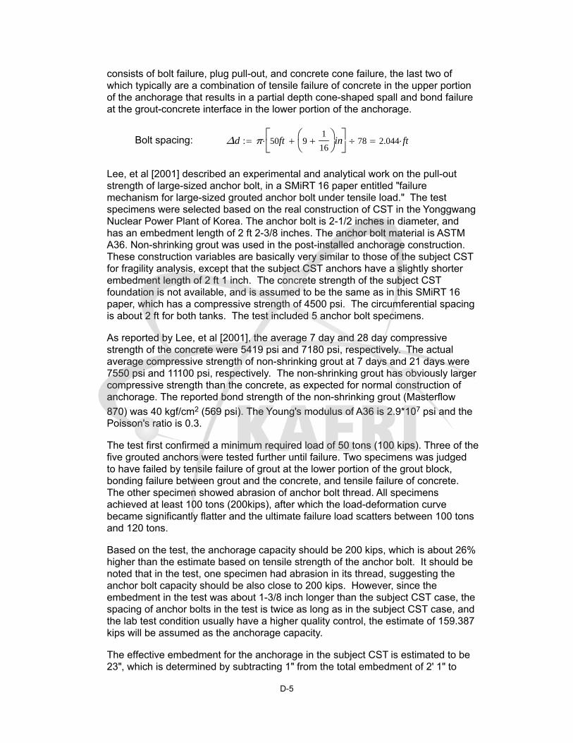
consists of bolt failure, plug pull-out, and concrete cone failure, the last two ofwhich typically are a combination of tensile failure of concrete in the upper portionof the anchorage that results in a partial depth cone-shaped spall and bond failureat the grout-concrete interface in the lower portion of the anchorage.

Bolt spacing: Δd π 50ft 91

16

in

78 2.044 ft

Lee, et al [2001] described an experimental and analytical work on the pull-outstrength of large-sized anchor bolt, in a SMiRT 16 paper entitled "failuremechanism for large-sized grouted anchor bolt under tensile load." The testspecimens were selected based on the real construction of CST in the YonggwangNuclear Power Plant of Korea. The anchor bolt is 2-1/2 inches in diameter, andhas an embedment length of 2 ft 2-3/8 inches. The anchor bolt material is ASTMA36. Non-shrinking grout was used in the post-installed anchorage construction.These construction variables are basically very similar to those of the subject CSTfor fragility analysis, except that the subject CST anchors have a slightly shorterembedment length of 2 ft 1 inch. The concrete strength of the subject CSTfoundation is not available, and is assumed to be the same as in this SMiRT 16paper, which has a compressive strength of 4500 psi. The circumferential spacingis about 2 ft for both tanks. The test included 5 anchor bolt specimens.

As reported by Lee, et al [2001], the average 7 day and 28 day compressivestrength of the concrete were 5419 psi and 7180 psi, respectively. The actualaverage compressive strength of non-shrinking grout at 7 days and 21 days were7550 psi and 11100 psi, respectively. The non-shrinking grout has obviously largercompressive strength than the concrete, as expected for normal construction ofanchorage. The reported bond strength of the non-shrinking grout (Masterflow

870) was 40 kgf/cm2 (569 psi). The Young's modulus of A36 is 2.9*107 psi and thePoisson's ratio is 0.3.

The test first confirmed a minimum required load of 50 tons (100 kips). Three of thefive grouted anchors were tested further until failure. Two specimens was judgedto have failed by tensile failure of grout at the lower portion of the grout block,bonding failure between grout and the concrete, and tensile failure of concrete.The other specimen showed abrasion of anchor bolt thread. All specimensachieved at least 100 tons (200kips), after which the load-deformation curvebecame significantly flatter and the ultimate failure load scatters between 100 tonsand 120 tons.

Based on the test, the anchorage capacity should be 200 kips, which is about 26%higher than the estimate based on tensile strength of the anchor bolt. It should benoted that in the test, one specimen had abrasion in its thread, suggesting theanchor bolt capacity should be also close to 200 kips. However, since theembedment in the test was about 1-3/8 inch longer than the subject CST case, thespacing of anchor bolts in the test is twice as long as in the subject CST case, andthe lab test condition usually have a higher quality control, the estimate of 159.387kips will be assumed as the anchorage capacity.

The effective embedment for the anchorage in the subject CST is estimated to be23", which is determined by subtracting 1" from the total embedment of 2' 1" to

D-5

account for the nuts.

heff 23in

The compressive strength of the concrete is assumed to be 4500 psi, accordingto the above mentioned paper. It should be pointed out that the measuredstrength in the test is higher.

f'c 4500psi

Base case of the anchor bolt strength based on concrete based onNUREG/CR-5434 (Figure 5.20):

k 57

TAC kheff

in

1.5

f'c

psi lbf 421.767 kips

Note that this TAC capacity calculated based on NUREG/CR-5434 is greater than

200 kips as determined in the test as reported in a SMiRT paper by Lee, et al.[2001]. The anchor bolts in the tests reported in NUREG/CR-5434 have a diameterof 3/4" and an embedment of 4", which are much smaller than those used in the CSTconstruction. Therefore, the test data in NUREG/CR-5434 will be used as factors toscale the test data as reported in the paper by Lee, et al. [2001].

fTAC200kips

421.767kips0.474

Strengths for a crack width of 0mm and 0.3 mm can be assumed to be, based onFigure 5.20 of NUREG/CR-5434:

TAC_00 200kips

TAC_03 200kips15.5

57 54.386 kips

TAC as a function of crack width can be established as:

TAC c( ) max TAC_00c

0.3mmTAC_03 TAC_00 0kips

TAC crack( ) 101.187 kips

TBC 159.387 kips

TBC min TBC TAC crack( ) 101.187 kips

D-6

H.3.3 Fluid Hold-down Forces:

Schematic Illustration of Tank Bottom Behavior NearTensile Region of Tank Shell [NUREG/CR-5270]

The hold-down force Te increases with increasing fluid pressure P, which

consequently assumes the minimum tension zone fluid press PT-. A number of

other related parameters are also defined below.

P PT- 3.288 psi

ν 0.3tS 0.625 in

Ib

tB3

12 1 ν2 1.917 10

3 in3

tB 7 mm

KES tS

3

12 1 ν2 7.325 10

4 J

κR

tS3 1 ν

2

0.5

28.177

MFPR tS

12 1 ν2

1R

H κ

0.036m2 MFP is a shortcut to MF / P

D-7

KS2 K κ

R5.412 10

5 N

The uplift height δe, the hold down tension Te, moment Me, rotation ae, and

maximum positive moment M+ can then be defined as functions of uplift length l:

F l( ) 1KS l

2ES Ib

δe l( )l4

24

1

F l( )

KS l5

72ES IbMFP

l2

6

P

ES Ib

Note: this equation as in theoriginal CDFM method issingular at L= 0 ft. The MFP/Lterm only has a minor effect onTe when L is very small. The

linear approximation in theoriginal CDFM method caneffectively avoid thissingularity.

Te l( ) Pl

2

1

F l( )

KS l2

12ES IbMFP

l

Me l( ) P1

F l( )

KS l

3

12ES IbMFP

The singularity in this equationcan be similarly avoided by thelinear approximation.

M+ l( ) Pl2

8

Me l( )

2P

Me l( )2

2P2

l2

αe l( )P l

312ES Ib

Me l( ) l

2ES Ib

Given

l 0in

l2

24

1

F l( )

KS l3

72ES IbMFP

1

6

0=

D-8

lmin Find l( ) 7.65 in

Given

lmax 10in

δe lmax( ) 0.165in=

lmax Find lmax( ) 21.061 in

l lmin lmin 0.1in lmax

Linear Approximation:

i 0lmax lmin( )

0.1in

l_veci lmin i 0.1 in

Te0

Te1

lineδe l_vec( )

in

Te l_vec( )in

lbf

24.007

162.111

Te0 if PT- 0psi Te0 0 lbf

in24.007

lbf

in

Te1 if PT- 0psi Te1 0 lbf

in2

162.111lbf

in2

Te_lin δe Te0 Te1 δe

D-9

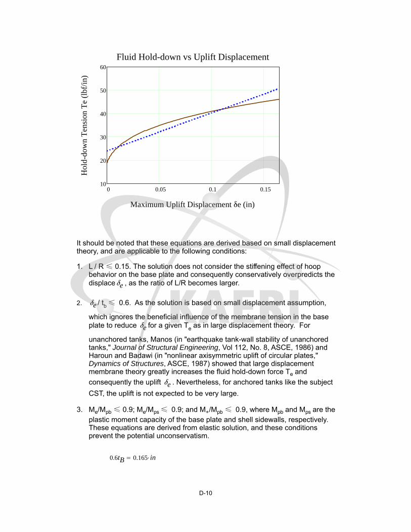
0 0.05 0.1 0.1510

20

30

40

50

60

Fluid Hold-down vs Uplift Displacement

Maximum Uplift Displacement δe (in)

Hol

d-do

wn

Ten

sion

Te

(lbf

/in)

It should be noted that these equations are derived based on small displacementtheory, and are applicable to the following conditions:

L / R ≤ 0.15. The solution does not consider the stiffening effect of hoop1.behavior on the base plate and consequently conservatively overpredicts thedisplaceδe , as the ratio of L/R becomes larger.

δe / tb ≤ 0.6. As the solution is based on small displacement assumption,2.

which ignores the beneficial influence of the membrane tension in the baseplate to reduce δe for a given Te as in large displacement theory. For

unanchored tanks, Manos (in "earthquake tank-wall stability of unanchoredtanks," Journal of Structural Engineering, Vol 112, No. 8, ASCE, 1986) andHaroun and Badawi (in "nonlinear axisymmetric uplift of circular plates,"Dynamics of Structures, ASCE, 1987) showed that large displacementmembrane theory greatly increases the fluid hold-down force Te and

consequently the uplift δe . Nevertheless, for anchored tanks like the subject

CST, the uplift is not expected to be very large.

Me/Mpb ≤ 0.9; Me/Mps ≤ 0.9; and M+/Mpb ≤ 0.9, where Mpb and Mps are the3.plastic moment capacity of the base plate and shell sidewalls, respectively.These equations are derived from elastic solution, and these conditionsprevent the potential unconservatism.

0.6tB 0.165 in

D-10

The second requirement leads to maximum δe of 0.165 in, beyond which the small

displacement theory becomes increasingly conservative. The original CDFM solvedthe problem by making a linear approximation of the δe-Te curve in a range of δe=0

to 0.6tB, and then use the linear equation to extrapolate beyond the 0.6tB to partiallyaccount for membrane tension effects. This approach will also be used in thisstudy.

Te Te_lin

Assessment of the upper limit on the fluid hold-down force: based on a yieldstress σy of 30 ksi, and an ultimate stress of 75 ksi, the fully plastic moment

capacity Mpb of the 7 mm base plate is estimated to be 0.949 kips-inch/inch when

the outer fiber reaches 75 ksi. It is also assumed that the effective hoopcompressive yield stress σye is equal to 45 ksi. The upper limit of the horizontal

component of the membrane tension FH can be found to be:

σye 45 ksi

Mpb

tB3

12

tB

2

75 ksi 0.949kips in

in

FH

σye tS

2κ

Mpb κ

R 0.588

kips

in

4MpbPT- 0.5111.742

lbf

in

FH

2Mpb0.31

1

in

Thus, the upper limit of the fluid hold-down force is estimated to be:

Tm δe 168.841lbf

in1

0.31 δe

in

0.5

The maximum δe can be found by equating Te and Tm:

Given

δee 0.15in

Te δee Tm δee =

δee Find δee 1.051 in

D-11

Therefore, the linearized equation for Te should not be extrapolated beyond δe =

1.805 inch.

Note that linearization is necessary later when developing overturning momentcapacity.

H.3.4 Overturning Moment Capacity:

Vertical Loading on Tank Shell at Base [NUREG/CR-5270]

The overturning moment capacity MSC can be estimated using the compressive

buckling capacity of the tank shell (CB), the anchor bolt hold-down capacity

(TBC), and the relationship between fluid hold-down force and uplift

D-12

displacement. The estimation approach in the CDFM method requires severalconservative but reasonable assumptions as noted below:

The bottom of the tank shell is assumed to rotate rigidly about the1.neutral axis (plane sections remain plane).

The cross-section of the tank at the top of the top plate of the bolt2.chairs (hc above the base) is assumed to remain horizontal so that all

vertical tank distortions needed to result in base uplift andmobilization of the anchor bolts must be accommodated over theheight hc.

The compressive stress varies linearly from zero at the neutral axis3.(α=β as in the figure above) to its maximum value Cm at α=180°, as

given by Cm = Estsδc/hc ≤ CB (by converting eq. H-39), where δc is

the maximum compressive shortening.

Summary of parameters:

Cm 12.072kips

in TBC 101.187 kips

Te0 0.024kips

in Te1 0.162

kips

in2

WTe 176.395 kips AB Abolt AB 4.909 in2

EB 29 103ksi

R 25.026 ft

ts 0.625 in Es ES 29 103 ksi

hc 207mm 8.15 in

ha 2ft 1in 25 in

Using the approach outlined in NUREG/CR-5270 instead of the EPRINP-6041-SL appendix H in the following:

δc

Cm hc

Es ts5.428 10

3 in

KB

δc AB EB

ha hc23.31 kips

ΔTe Te1 δc 8.8 104

kips

in

D-13

δea a b( ) δccos a( ) cos b( )

1 cos b( )

Because the bolt pretension TBP is unreliable after a number of years in service, it

is conservatively assumed to be 0.

TBP 0kips

The neutral axis angle β can be determined iteratively using the followingprocedure.

Bolt locations: i 0 77

αi2π

78i

Tfunc α β( ) c TBP KBcos α( ) cos β( )

1 cos β( )

c TBC c TBCif

c 0 c 0if

C1 β( )1 cos β( )

sin β( ) π β( )cos β( )

C2 β( )sin β( ) cos β( ) π β

1 cos β( )

C3 β( )sin β( ) β cos β( )

sin β( ) π β( )cos β( )

C4 β( )β sin β( ) cos β( )

1 cos β( )

TB α β( ) Tfunc α β( )

Cf'm α β( )

WTe TB α β( )2R

Te0 β

C1 β( ) ΔTe C3 β( )

Equating Cf'm and Cm to determine β:

func α β( ) Cf'm α β( ) Cm

β root func α β( ) β 0 3.1( )

D-14

β 2.302 β180

π 131.895

C'm Cf'm α β( ) 12.072kips

in Cm 12.072

kips

in

Use C'm and β to find the overturning moment capacity MSC:

MSC C'm C2 β( ) R2 TB α β( ) R cos α( )

Te0 R2 2 sin β( ) ΔTe C4 β( ) R

2

MSC 150617.311 kips ft

TB α β( ) 3.796 103 kips

The largest bolt elongation (at α=0) should be checked to ensure that theanchorage has the capability:

δe0 δea α0 β 0.027 in

Elongation ratio:δe0

ha hc0.082 %

The maximum elongation ratio is much smaller than 1%, which is recommended inthe original CDFM method for the A307 bolt. One percent is also considered to be anappropriate percentage value for the A36 anchor bolt used in the subject CSTconstruction.

The maximum tank shell uplift distortion δe0 = 0.026 in, which is much less than the

limit of 0.165 in for the small displacement theory to be applicable in developing thefluid hold-down capacity.

Because there are 78 anchor bolts (the example tank in the original CDFM methodhad only 8), the case where α=0 lies midway between bolts need not be checked.

The uncertainty in HCLPF buckling capacity of the tank shell due to the uncertainσye can lead to an MSC as low as 119133.414 kips-ft or as high as 192156.702

kips-ft. It should be noted that unlike in the original CDFM method, MSC is sensitive

to the estimate of Cm.

Inelastic energy absorption reduction factor k can be applied to linearly computedseismic response to obtain the actual overturning moment capacity. The combinedbolt yielding and tank shell buckling failure mode for overturning moment is not brittleso that k can be less than unity. However, as stated in the original CDFM method, itis difficult to make an appropriate estimate of k for this failure mode. Therefore, it is

D-15

conservatively assumed to be unity.

k 1.0

SMEM

MSC

k MSHSMEe SMEM 1.115 g

Since SMEM is substantially different from SMEe, the above procedure should be

iterated to obtain the appropriate SME estimate. The resultant SMEe is found to be

0.97g.

H.3.5 Sliding Capacity:

The base plate of the CST has a slight cone ( with a slope of 1 to 96) so that thefluid will always drain away from the center of the tank. This cone is generallycreated by variable thickness of the oiled sand cushion between the tank bottomplate and its foundation. Therefore, the coefficient of friction between the tankbase and its foundation is reasonably assumed to have a conservative value of0.55:

COF 0.55

The sliding shear capacity can then be calculated as,

VSC COF WTe Pa π R2 TB α β( )

3.835 103 kips

The shear capacity of the bolts should not be considered because (a) there is alarge space between the concrete foundation and the anchor bolt chair, and (b)there is a 1/4" diametric clearance in the hole in the anchor bolt chair.

The sliding capacity with a unit inelastic absorption factor as suggested by theoriginal CDFM method:

SMEV

VSC

k VSHSMEe SMEV 0.423 g

By varying SMEe, the HCLPF shear capacity is found to be 0.555g.

Unlike the example tank in the original CDFM method, the capacity of the CSTappears to be governed by the sliding capacity. The sliding capacity considers onlythe friction between the bottom plate and the foundation.

D-16

H.3.6 Fluid Pressure Capacity:

The inelastic energy absorption seismic response reduction factor kμ is suggested

to be 0.8 for HCLPF capacity evaluation:

ku 0.8

For the CDFM hoop membrane stress capacity, it is recommended that the ASMEseismic design limit of 2 SM for primary stress should be used, which is 37.5 ksi for

SA240-type 304 stainless steel:

σa 37.5ksi

The pressure capacity, PCA, at the bottom of the tank shell (the CST has a uniform

shell thickness), can be estimated to be:

PCA t( )σa t

R

PCA tS 78.044 psi

The maximum seismic induced hydrodynamic pressures PSM and the hydrostatic

pressure PST at the bottom of the tank shell are:

PSM H( ) 1.098 105 Pa

PST H( ) 1.12 105 Pa

The HCLPF fluid pressure capacity SMEP can be determined as:

SMEp

PCA tS PST H( )

ku PSM H( )SMEe 2.052 g

By varying SMEe, the HCLPF fluid pressure capacity can be found to be 2.191 g,which does not govern. This agrees with seismic experience that the fluidpressure capacity seldom appears to govern the seismic capacity for normal flatbottomed steel tanks with butt-welded side plates.

Summary of SME capacities:

SMEM 1.115 g

SMEV 0.423 g

D-17

SMEp 2.052 g

SMEcr min SMEM SMEV SMEp 0.423 g

SMEe 0.423 g

if SMEcr SMEM= "Moment" if SMEcr SMEV= "Shear" "Fluid Pressure" "Shear"

crack 0.204 mm

Summary of results:

Years: 0 5 10 15 20 25 30 35 40cr (mm): 0.108 0.114 0.120 0.126 0.132 0.138 0.144 0.150 0.156SME: 0.426 0.426 0.426 0.426 0.426 0.426 0.426 0.426 0.426SMEM: 1.140 1.140 1.140 1.140 1.140 1.140 1.140 1.140 1.140SMEV: 0.426 0.426 0.426 0.426 0.426 0.426 0.426 0.426 0.426SMEP: 2.052 2.052 2.052 2.052 2.052 2.052 2.052 2.052 2.052Mode: Shear Shear Shear Shear Shear Shear Shear Shear Shear

Years: 45 50 55 60 65 70 75 80cr (mm): 0.162 0.168 0.174 0.180 0.186 0.192 0.198 0.204SME: 0.426 0.426 0.426 0.426 0.425 0.425 0.424 0.423SMEM: 1.140 1.140 1.140 1.140 1.137 1.131 1.124 1.115SMEV: 0.426 0.426 0.426 0.426 0.425 0.425 0.424 0.423SMEP: 2.052 2.052 2.052 2.052 2.052 2.052 2.052 2.052Mode: Shear Shear Shear Shear Shear Shear Shear Shear

H.3.7 Consideration of Other Capacities:

(1) Slosh height for roof damage: note that even with a SMEe = 0.334 g (the initial

guess), the slosh height is about 4.8 ft. With the HCLPF shear capacity of

SMEe=0.555 g, the sloshing height can be about 7.9 ft, which is close to the total

height of the head (8.7', as approximated in the beginning part of this calculation).

hs 6.05 ft SMEe 0.423 g

The increase of sloshing height is not significant as SMEe increases from 0.334 gto 0.555 g. In addition, as pointed out in the original CDFM method, even if roofdamage might be expected, such damage usually does not impair the ability of thetank to contain fluid.

(2) The CST is assumed to sit on rock/very stiff soil; therefore, soil-tankfoundation interaction is not considered.

(3) Piping failure or failure of nozzles may lead to loss of fluid in the tank, andmore importantly, may impair the normal function of the condensation system. Asreported in the original CDFM method, a significant fraction of the cases ofseismic induced loss of tank contents have been due to piping/nozzle failuresbecause of poor detailing. The CDFM method also stated that a SME evaluation

D-18

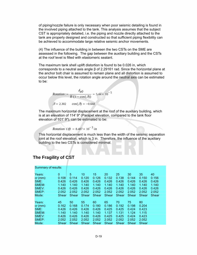
of piping/nozzle failure is only necessary when poor seismic detailing is found inthe involved piping attached to the tank. This analysis assumes that the subjectCST is appropriately detailed, i.e. the piping and nozzle directly attached to thetank are properly designed and constructed so that sufficient piping flexibility canbe achieved to accommodate large relative seismic anchor movements.

(4) The influence of the building in between the two CSTs on the SME areassessed in the following. The gap between the auxiliary building and the CSTsat the roof level is filled with elastomeric sealant.

The maximum tank shell uplift distortion is found to be 0.026 in, whichcorresponds to a neutral axis angle β of 2.29161 rad. Since the horizontal plane atthe anchor bolt chair is assumed to remain plane and all distortion is assumed tooccur below this level, the rotation angle around the neutral axis can be estimatedto be:

Rotationδe0

R 1 cos β( )( )5.44 10

5

β 2.302 cos β( ) 0.668

The maximum horizontal displacement at the roof of the auxiliary building, whichis at an elevation of 114' 9" (Parapet elevation, compared to the tank floorelevation of 101' 9"), can be estimated to be:

Rotation 13 ft 8.487 103 in

This horizontal displacement is much less than the width of the seismic separationjoint at the roof elevation, which is 3 in. Therefore, the influence of the auxiliarybuilding to the two CSTs is considered minimal.

The Fragility of CST

Summary of results:

Years: 0 5 10 15 20 25 30 35 40cr (mm): 0.108 0.114 0.120 0.126 0.132 0.138 0.144 0.150 0.156SME: 0.426 0.426 0.426 0.426 0.426 0.426 0.426 0.426 0.426SMEM: 1.140 1.140 1.140 1.140 1.140 1.140 1.140 1.140 1.140SMEV: 0.426 0.426 0.426 0.426 0.426 0.426 0.426 0.426 0.426SMEP: 2.052 2.052 2.052 2.052 2.052 2.052 2.052 2.052 2.052Mode: Shear Shear Shear Shear Shear Shear Shear Shear Shear

Years: 45 50 55 60 65 70 75 80cr (mm): 0.162 0.168 0.174 0.180 0.186 0.192 0.198 0.204SME: 0.426 0.426 0.426 0.426 0.425 0.425 0.424 0.423SMEM: 1.140 1.140 1.140 1.140 1.137 1.131 1.124 1.115SMEV: 0.426 0.426 0.426 0.426 0.425 0.425 0.424 0.423SMEP: 2.052 2.052 2.052 2.052 2.052 2.052 2.052 2.052Mode: Shear Shear Shear Shear Shear Shear Shear Shear

D-19

SMEHCLPF 0.426 0.426 0.426 0.426 0.426 0.426 0.426 0.426 0.426 0.426 0.42(

SMEM 1.140 1.140 1.140 1.140 1.140 1.140 1.140 1.140 1.140 1.140 1.140 1.1(

SMEV 0.426 0.426 0.426 0.426 0.426 0.426 0.426 0.426 0.426 0.426 0.426 0.4(

SMEP 2.052 2.052 2.052 2.052 2.052 2.052 2.052 2.052 2.052 2.052 2.052 2.0(

It should be emphasized that the HCLPF SME capacity assumes the RegulatoryGuide 1.60 spectra anchored to the HCLPF SME PGA.

To determine the seismic fragility of the CST, one needs to convert the HCLPFSME PGA to median SME PGA. This conversion requires the estimate of bothaleatory and epistemic uncertainties (βR and βU). The Fragility Method, also

presented along with the original CDFM method, estimates the aleatory andepistemic uncertainties to be 0.2 and 0.27, respectively. These uncertainties arenearly identical to those reported by Choun, et al [2008]. The SME median SMEm

can then be estimated as well.

i 0 1 16

βR 0.2

βU 0.27

βC βR2

βU2 0.336

Hm exp 1.645 βR βU 2.167

SMEmiSMEHCLPFi

Hm

SMEMmiSMEMi

Hm

SMEVmiSMEVi

Hm

SMEPmiSMEPi

Hm

D-20

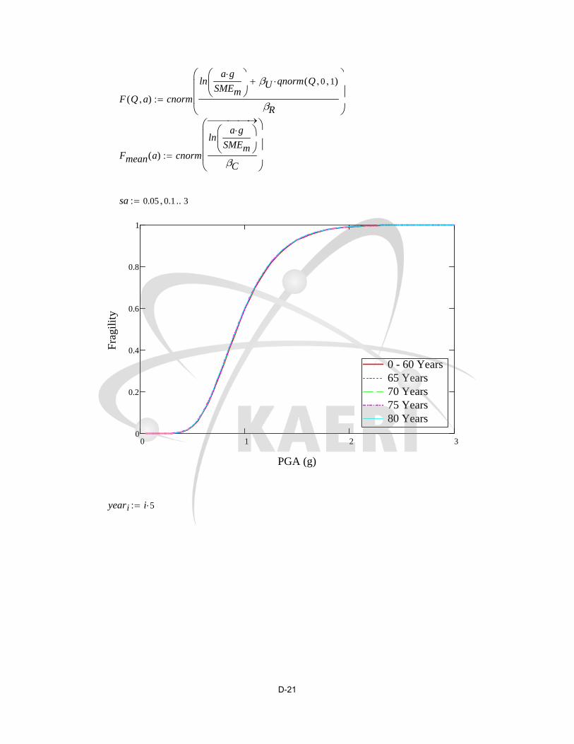
F Q a( ) cnorm

lna g

SMEm

βU qnorm Q 0 1( )

βR

Fmean a( ) cnorm

lna g

SMEm

βC

sa 0.05 0.1 3

0 1 2 30

0.2

0.4

0.6

0.8

1

0 - 60 Years65 Years70 Years75 Years80 Years

PGA (g)

Fra

gili

ty

yeari i 5

D-21

0 20 40 60 800

0.5

1

1.5

2

2.5

HCLPF CapacityOverturning Moment CapacitySliding CapacityFluid Pressure Capacity

Time (year)

HC

LP

F F

ragi

lity

Cap

acit

y (g

)

D-22

0 20 40 60 800

1

2

3

4

5

Median CapacityOverturning Moment CapacitySliding CapacityFluid Pressure Capacity

Time (year)

Med

ian

Fra

gili

ty C

apac

ity

(g)

D-23

26 0.426 0.426 0.425 0.425 0.424 0.423 )T

g

140 1.140 1.137 1.131 1.124 1.115 )T

g

426 0.426 0.425 0.425 0.424 0.423 )T

g

52 2.052 2.052 2.052 2.052 2.052 )T

g

D-24

Appendix E FRAGILITY ANALYSIS OF THE CST WITH FOUNDATION CONCRETE CRACKING – APPLICATION OF MODEL C-2

KAERI Year 3 Task

Fragility Analysis of Condensate Storage Tank

- Degradation Case (C-2) Anchorage (concrete)Degradation

This case utilizes the concrete degradation data recorded in Korea NPPs and testdata of dynamic anchorage strength with simulated cracks in concrete as reported inNUREG/CR-5434.

The anchorage strength is the smaller of the bolt strength (base case) and theanchorage strength attributed to concrete with various levels of degradation.

The grouted anchors used NURE/CR-5434 have a diameter of 3/4" and (effective)embedment of 4". Both dimensions are much smaller than the anchorage in the CSTconstruction. Therefore, the data in NUREG/CR-5434 will be used as scaling factors.

Crack width regression curve developed by BNL based on KAERI data is used topredict the crack width.

year 80

crack 0.0078 year mm 0.624 mm

H.1 Introduction

KAERI indicated that the seismic DBE in Korea follows the NRC Reg. Guide 1.60design spectrum shape but with a PGA level scaled down to 0.2 g. An initial HCLPFcapacity was assumed to be 1.67 times of 0.2 g. However, since the Mathcadsheets in this appendix solve the various equations iteratively by manually settingSMEe to different values, the following SMEe value of 0.165 g represents the

converged solution for the degradation level of the anchorage (concrete) at 80 years.

SMEe 0.165g

H.2 Response Evaluation

Same as Appendix A, Section H.2.

E-1

H.3 Capacity Assessment

The seismic overturning moment capacity of the CST at its base, MSC, depends

on the axial compressive buckling capacity of the tank shell Cm, the tensile

hold-down capacity of the anchor bolts including their anchorage and attachmentto the tank TBC, and the hold-down capacity of the fluid pressure acting on the

tank base plate Te.

Although unlikely for larger radius tanks, the tank SME capacity is sometimesgoverned by the sliding shear capacity at the tank base, VSC. Even though it does

not appear that any butt welded steel tank has ever failed due to seismic inducedmembrane hoop stresses due to combined hydrostatic and hydrodynamic fluidpressures, the SME capacity of this failure mode, PCA, should also be checked.

Additional assessment of the seismic capacity may include the possibility andconsequence of the fluid sloshing against the tank roof, foundation failure for soilsites, and possibility of failure of piping or their attachment to the tank.

H.3.1 Compressive Buckling Capacity of the Tank Shell:

The most likely buckling for tanks is the "elephant-foot" buckling near the base ofthe tank shell. The "elephant-foot" buckling is a combined effect of hoop tension,axial (vertical) compression, and restriction of radial deformation of the tank shellby the base plate. "Elephant-foot" buckling does not necessarily lead to failure of atank (e.g., leakage). However, there is no simple capability evaluation method thatcan predict tank performance after the development of "elephant-foot" buckling.Therefore, for a CDFM SME capacity of tanks, the onset of "elephant-foot"buckling will be judged to represent the limit to the compressive buckling capacityof the tank shell. The onset of "elephant-foot" buckling can be estimated usingelastic-plastic collapse theory as presented in the following:

The sidewall thickness near the shell base: ts tS 0.625 in

The tank internal pressure near its base: P PC+ 1.469 105 Pa

Elastic modulus of the tank: ES 2.9 104 ksi

The CST shell was made of SA 204-type 304 stainless steel. This material doesnot have a flat yield plateau and as strain increases its stress can grow to aminimum ultimate stress capacity of 75 ksi. In the CDFM method, an effective yieldstress σye is set to 2.4SM or 45 ksi, in line with the ASME seismic design limit for

primary local membrane plus primary bending [ASME 1983, "ASME Boiler &Pressure Vessel Code"]. The potential uncertainty range for σye is reported to be

between 30 ksi and 60 ksi, according to the original CDFM method description.

E-2

σye 45ksi

R

ts480.5

S1R

ts400 1.201

The "elephant-foot" buckling axial stress of the tank shell can be accuratelypredicted to be:

σp

0.6ES

R ts1

P Rσye ts

2

11

1.12 S11.5

S1

σye

36ksi

S1 1

22.545 ksi

The compressive buckling capacity for HCLPF capacity computation utilizes arecommended 0.9 reduction factor of the buckling stress:

Cm 0.9σp ts 12.681kips

in

Buckling capacity of the supported cylindrical shells under combined axial bendingand internal pressure should also be checked although it is unlikely to govern foroverall seismic response of fluid containing tanks. The axial bending inducedbuckling stress, σCB, for such a load case can be conservatively estimated(essentially lower bound) as follows.

A parameter Δγ to be used in the following procedure as an increase factor forinternal pressure can be obtained from Figure 6 of "Buckling of Thin-walledCircular Cylinders", [NASA SP-8007]. Δγ depends on the minimum compressionzone pressure at the base of the tank shell, PC-, corresponding to the time ofmaximum moment.

Considering the potential range on σye of 30 to 60 ksi, the resultant range on σp is16.572 ksi to 26.702 ksi. Consequently, Cm has a range of 9.322 kips/in to 15.02kips/in.

PC-

ES

R

tS

2

0.134

From Figure 6 of NASA SP-8007: Δγ 0.12

ϕ1

16

R

ts 1.37

E-3

γ 1 0.73 1 eϕ 0.455

σCB 0.6γ Δγ( )ES

R ts23.737 ksi

0.9σp 20.29 ksi

σCB exceeds 0.9sp, so it does not govern.

H.3.2 Bolt Hold-down Capacity:

The bolt hold-down capacity should be determined as the smallest of the bolttensile capacity, anchorage of bolt into concrete foundation, capacity of the topplate of bolt chairs to transfer bolt loads to the vertical chair gussets, attachment ofthe top plate and vertical chair gussets to the tank shell, and the capacity of tankshell to withstand concentrated loads imposed on it by bolt chairs.

Anchor bolt capacity: the anchor bolt has a diameter of 2 1/2" and is made of A36steel. The tensile capacity can be determined as:

dbolt 2.5in

Abolt

π dbolt2

44.909 in

2

Based on the AISC Code [9th edition, 1989] for threaded A36 bolts:

TBC 1.7Abolt 19.1 ksi 159.387 kips TBC 79.693 tonf

Note that TBC is the capacity of one bolt and the capacity of the interacting

multi-bolts will be considered later.

Anchor bolt chair capacity check: according to the drawing, the anchor boltchairs form a circumferentially continuous construction. Based on the continuouschair construction and the sizing of the plates and weld, it is judged that the anchorbolt chair and its attachment to the tank shell is adequate to transfer the boltcapacity load for the CST tank. The tank shell is also considered to be adequatein withstanding the concentrated loads imposed on it by bolt chairs, especiallybecause the "elephant-foot" buckling capacity is also checked.

tchair 13

8

in 1.375 in

Weld width is 15 mm (5/8") according to the drawing.

Capacity of bolt anchorage into concrete foundation: the anchorage isconstructed using non-shrinking grout. The tensile failure of bolt anchorage mainly

E-4

consists of bolt failure, plug pull-out, and concrete cone failure, the last two ofwhich typically are a combination of tensile failure of concrete in the upper portionof the anchorage that results in a partial depth cone-shaped spall and bond failureat the grout-concrete interface in the lower portion of the anchorage.

Bolt spacing: Δd π 50ft 91

16

in

78 2.044 ft

Lee, et al [2001] described an experimental and analytical work on the pull-outstrength of large-sized anchor bolt, in a SMiRT 16 paper entitled "failuremechanism for large-sized grouted anchor bolt under tensile load." The testspecimens were selected based on the real construction of CST in the YonggwangNuclear Power Plant of Korea. The anchor bolt is 2-1/2 inches in diameter, andhas an embedment length of 2 ft 2-3/8 inches. The anchor bolt material is ASTMA36. Non-shrinking grout was used in the post-installed anchorage construction.These construction variables are basically very similar to those of the subject CSTfor fragility analysis, except that the subject CST anchors have a slightly shorterembedment length of 2 ft 1 inch. The concrete strength of the subject CSTfoundation is not available, and is assumed to be the same as in this SMiRT 16paper, which has a compressive strength of 4500 psi. The circumferential spacingis about 2 ft for both tanks. The test included 5 anchor bolt specimens.

As reported by Lee, et al [2001], the average 7 day and 28 day compressivestrength of the concrete were 5419 psi and 7180 psi, respectively. The actualaverage compressive strength of non-shrinking grout at 7 days and 21 days were7550 psi and 11100 psi, respectively. The non-shrinking grout has obviously largercompressive strength than the concrete, as expected for normal construction ofanchorage. The reported bond strength of the non-shrinking grout (Masterflow

870) was 40 kgf/cm2 (569 psi). The Young's modulus of A36 is 2.9*107 psi and thePoisson's ratio is 0.3.

The test first confirmed a minimum required load of 50 tons (100 kips). Three of thefive grouted anchors were tested further until failure. Two specimens was judgedto have failed by tensile failure of grout at the lower portion of the grout block,bonding failure between grout and the concrete, and tensile failure of concrete.The other specimen showed abrasion of anchor bolt thread. All specimensachieved at least 100 tons (200kips), after which the load-deformation curvebecame significantly flatter and the ultimate failure load scatters between 100 tonsand 120 tons.

Based on the test, the anchorage capacity should be 200 kips, which is about 26%higher than the estimate based on tensile strength of the anchor bolt. It should benoted that in the test, one specimen had abrasion in its thread, suggesting theanchor bolt capacity should be also close to 200 kips. However, since theembedment in the test was about 1-3/8 inch longer than the subject CST case, thespacing of anchor bolts in the test is twice as long as in the subject CST case, andthe lab test condition usually have a higher quality control, the estimate of 159.387kips will be assumed as the anchorage capacity.

The effective embedment for the anchorage in the subject CST is estimated to be23", which is determined by subtracting 1" from the total embedment of 2' 1" to

E-5

account for the nuts.

heff 23in

The compressive strength of the concrete is assumed to be 4500 psi, accordingto the above mentioned paper. It should be pointed out that the measuredstrength in the test is higher.

f'c 4500psi

Base case of the anchor bolt strength based on concrete based onNUREG/CR-5434 (Figure 5.20):

k 57

TAC kheff

in

1.5

f'c

psi lbf 421.767 kips

Note that this TAC capacity calculated based on NUREG/CR-5434 is greater than

200 kips as determined in the test as reported in a SMiRT paper by Lee, et al.[2001]. The anchor bolts in the tests reported in NUREG/CR-5434 have a diameterof 3/4" and an embedment of 4", which are much smaller than those used in theCST construction. Therefore, the test data in NUREG/CR-5434 will be used asfactors to scale the test data as reported in the paper by Lee, et al. [2001].

fTAC200kips

421.767kips0.474

Strengths for a crack width of 0mm and 0.3 mm can be assumed to be, based onFigure 5.20 of NUREG/CR-5434:

TAC_00 200kips

TAC_03 200kips15.5

57 54.386 kips

TAC as a function of crack width can be established as:

TAC c( ) max TAC_00c

0.3mmTAC_03 TAC_00 0kips

TAC crack( ) 0 kips

TBC 159.387 kips

TBC min TBC TAC crack( ) 0 kips

E-6

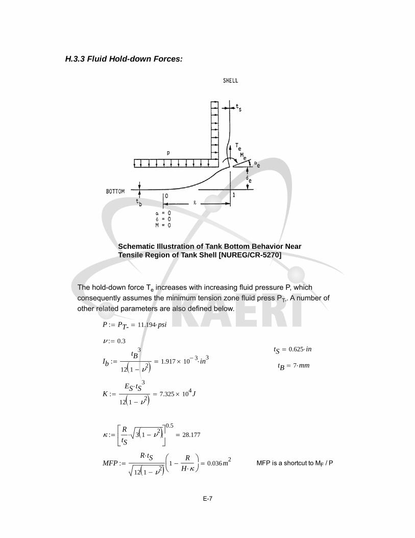
H.3.3 Fluid Hold-down Forces:

Schematic Illustration of Tank Bottom Behavior NearTensile Region of Tank Shell [NUREG/CR-5270]

The hold-down force Te increases with increasing fluid pressure P, which

consequently assumes the minimum tension zone fluid press PT-. A number of

other related parameters are also defined below.

P PT- 11.194 psi

ν 0.3tS 0.625 in

Ib

tB3

12 1 ν2 1.917 10

3 in3

tB 7 mm

KES tS

3

12 1 ν2 7.325 10

4 J

κR

tS3 1 ν

2

0.5

28.177

MFPR tS

12 1 ν2

1R

H κ

0.036m2 MFP is a shortcut to MF / P

E-7

KS2 K κ

R5.412 10

5 N

The uplift height δe, the hold down tension Te, moment Me, rotation ae, and

maximum positive moment M+ can then be defined as functions of uplift length l:

F l( ) 1KS l

2ES Ib

δe l( )l4

24

1

F l( )

KS l5

72ES IbMFP

l2

6

P

ES Ib

Note: this equation as in theoriginal CDFM method issingular at L= 0 ft. The MFP/Lterm only has a minor effect onTe when L is very small. The

linear approximation in theoriginal CDFM method caneffectively avoid thissingularity.

Te l( ) Pl

2

1

F l( )

KS l2

12ES IbMFP

l

Me l( ) P1

F l( )

KS l

3

12ES IbMFP

The singularity in this equationcan be similarly avoided by thelinear approximation.

M+ l( ) Pl2

8

Me l( )

2P

Me l( )2

2P2

l2

αe l( )P l

312ES Ib

Me l( ) l

2ES Ib

Given

l 0in

l2

24

1

F l( )

KS l3

72ES IbMFP

1

6

0=

E-8

lmin Find l( ) 7.65 in

Given

lmax 10in

δe lmax( ) 0.165in=

lmax Find lmax( ) 15.735 in

l lmin lmin 0.1in lmax

Linear Approximation:

i 0lmax lmin( )

0.1in

l_veci lmin i 0.1 in

Te0

Te1

lineδe l_vec( )

in

Te l_vec( )in

lbf

72.042

326.372

Te0 if PT- 0psi Te0 0 lbf

in72.042

lbf

in

Te1 if PT- 0psi Te1 0 lbf

in2

326.372lbf

in2

Te_lin δe Te0 Te1 δe

E-9

0 0.05 0.1 0.1560

80

100

120

140

Fluid Hold-down vs Uplift Displacement

Maximum Uplift Displacement δe (in)

Hol

d-do

wn

Ten

sion

Te

(lbf

/in)

It should be noted that these equations are derived based on small displacementtheory, and are applicable to the following conditions:

L / R ≤ 0.15. The solution does not consider the stiffening effect of hoop1.behavior on the base plate and consequently conservatively overpredicts thedisplaceδe , as the ratio of L/R becomes larger.

δe / tb ≤ 0.6. As the solution is based on small displacement assumption,2.

which ignores the beneficial influence of the membrane tension in the baseplate to reduce δe for a given Te as in large displacement theory. For

unanchored tanks, Manos (in "earthquake tank-wall stability of unanchoredtanks," Journal of Structural Engineering, Vol 112, No. 8, ASCE, 1986) andHaroun and Badawi (in "nonlinear axisymmetric uplift of circular plates,"Dynamics of Structures, ASCE, 1987) showed that large displacementmembrane theory greatly increases the fluid hold-down force Te and

consequently the uplift δe . Nevertheless, for anchored tanks like the subject

CST, the uplift is not expected to be very large.

Me/Mpb ≤ 0.9; Me/Mps ≤ 0.9; and M+/Mpb ≤ 0.9, where Mpb and Mps are the3.plastic moment capacity of the base plate and shell sidewalls, respectively.These equations are derived from elastic solution, and these conditionsprevent the potential unconservatism.

0.6tB 0.165 in

E-10

The second requirement leads to maximum δe of 0.165 in, beyond which the small

displacement theory becomes increasingly conservative. The original CDFM solvedthe problem by making a linear approximation of the δe-Te curve in a range of δe=0

to 0.6tB, and then use the linear equation to extrapolate beyond the 0.6tB to partiallyaccount for membrane tension effects. This approach will also be used in thisstudy.

Te Te_lin

Assessment of the upper limit on the fluid hold-down force: based on a yieldstress σy of 30 ksi, and an ultimate stress of 75 ksi, the fully plastic moment

capacity Mpb of the 7 mm base plate is estimated to be 0.949 kips-inch/inch when

the outer fiber reaches 75 ksi. It is also assumed that the effective hoopcompressive yield stress σye is equal to 45 ksi. The upper limit of the horizontal

component of the membrane tension FH can be found to be:

σye 45 ksi

Mpb

tB3

12

tB

2

75 ksi 0.949kips in

in

FH

σye tS

2κ

Mpb κ

R 0.588

kips

in

4MpbPT- 0.5206.177

lbf

in

FH

2Mpb0.31

1

in

Thus, the upper limit of the fluid hold-down force is estimated to be:

Tm δe 168.841lbf

in1

0.31 δe

in

0.5

The maximum δe can be found by equating Te and Tm:

Given

δee 0.15in

Te δee Tm δee =

δee Find δee 0.322 in

E-11

Therefore, the linearized equation for Te should not be extrapolated beyond δe =

1.805 inch.

Note that linearization is necessary later when developing overturning momentcapacity.

H.3.4 Overturning Moment Capacity:

Vertical Loading on Tank Shell at Base [NUREG/CR-5270]

The overturning moment capacity MSC can be estimated using the compressive

buckling capacity of the tank shell (CB), the anchor bolt hold-down capacity

E-12

(TBC), and the relationship between fluid hold-down force and uplift

displacement. The estimation approach in the CDFM method requires severalconservative but reasonable assumptions as noted below:

The bottom of the tank shell is assumed to rotate rigidly about the1.neutral axis (plane sections remain plane).

The cross-section of the tank at the top of the top plate of the bolt2.chairs (hc above the base) is assumed to remain horizontal so that all

vertical tank distortions needed to result in base uplift andmobilization of the anchor bolts must be accommodated over theheight hc.

The compressive stress varies linearly from zero at the neutral axis3.(α=β as in the figure above) to its maximum value Cm at α=180°, as

given by Cm = Estsδc/hc ≤ CB (by converting eq. H-39), where δc is

the maximum compressive shortening.

Summary of parameters:

Cm 12.681kips

in TBC 0 kips

Te0 0.072kips

in Te1 0.326

kips

in2

WTe 198.306 kips AB Abolt AB 4.909 in2

EB 29 103ksi

R 25.026 ft

ts 0.625 in Es ES 29 103 ksi

hc 207mm 8.15 in

ha 2ft 1in 25 in

Using the approach outlined in NUREG/CR-5270 instead of the EPRINP-6041-SL appendix H in the following:

δc

Cm hc

Es ts5.702 10

3 in

KB

δc AB EB

ha hc24.486 kips

E-13

ΔTe Te1 δc 1.861 103

kips

in

δea a b( ) δccos a( ) cos b( )

1 cos b( )

Because the bolt pretension TBP is unreliable after a number of years in service, it

is conservatively assumed to be 0.

TBP 0kips

The neutral axis angle β can be determined iteratively using the followingprocedure.

Bolt locations: i 0 77

αi2π

78i

Tfunc α β( ) c TBP KBcos α( ) cos β( )

1 cos β( )

c TBC c TBCif

c 0 c 0if

C1 β( )1 cos β( )

sin β( ) π β( )cos β( )

C2 β( )sin β( ) cos β( ) π β

1 cos β( )

C3 β( )sin β( ) β cos β( )

sin β( ) π β( )cos β( )

C4 β( )β sin β( ) cos β( )

1 cos β( )

TB α β( ) Tfunc α β( )

Cf'm α β( )

WTe TB α β( )2R

Te0 β

C1 β( ) ΔTe C3 β( )

Equating Cf'm and Cm to determine β:

func α β( ) Cf'm α β( ) Cm

β root func α β( ) β 0 3.1( )

E-14

β 3.00419 β180

π 172.128

C'm Cf'm α β( ) 12.681kips

in Cm 12.681

kips

in

Use C'm and β to find the overturning moment capacity MSC:

MSC C'm C2 β( ) R2 TB α β( ) R cos α( )

Te0 R2 2 sin β( ) ΔTe C4 β( ) R

2

MSC 22230.13 kips ft

TB α β( ) 0 kips

The largest bolt elongation (at α=0) should be checked to ensure that theanchorage has the capability:

δe0 δea α0 β 1.204 in

Elongation ratio:δe0

ha hc3.633 %

Elongation assessment is valid here at the end of 80 years because the bolts attension will be pulled out. The following text is kept for other years.

The maximum elongation ratio is larger than 1%, which is recommended in theoriginal CDFM method for the A307 bolt. One percent is also considered to be anappropriate percentage value for the A36 anchor bolt used in the subject CSTconstruction.

The maximum tank shell uplift distortion δe0 = 0.026 in, which is much less than the

limit of 0.165 in for the small displacement theory to be applicable in developing thefluid hold-down capacity.

Because there are 78 anchor bolts (the example tank in the original CDFM methodhad only 8), the case where α=0 lies midway between bolts need not be checked.

The uncertainty in HCLPF buckling capacity of the tank shell due to the uncertainσye can lead to an MSC as low as 119133.414 kips-ft or as high as 192156.702

kips-ft. It should be noted that unlike in the original CDFM method, MSC is sensitive

to the estimate of Cm.

Inelastic energy absorption reduction factor k can be applied to linearly computedseismic response to obtain the actual overturning moment capacity. The combinedbolt yielding and tank shell buckling failure mode for overturning moment is not brittle

E-15

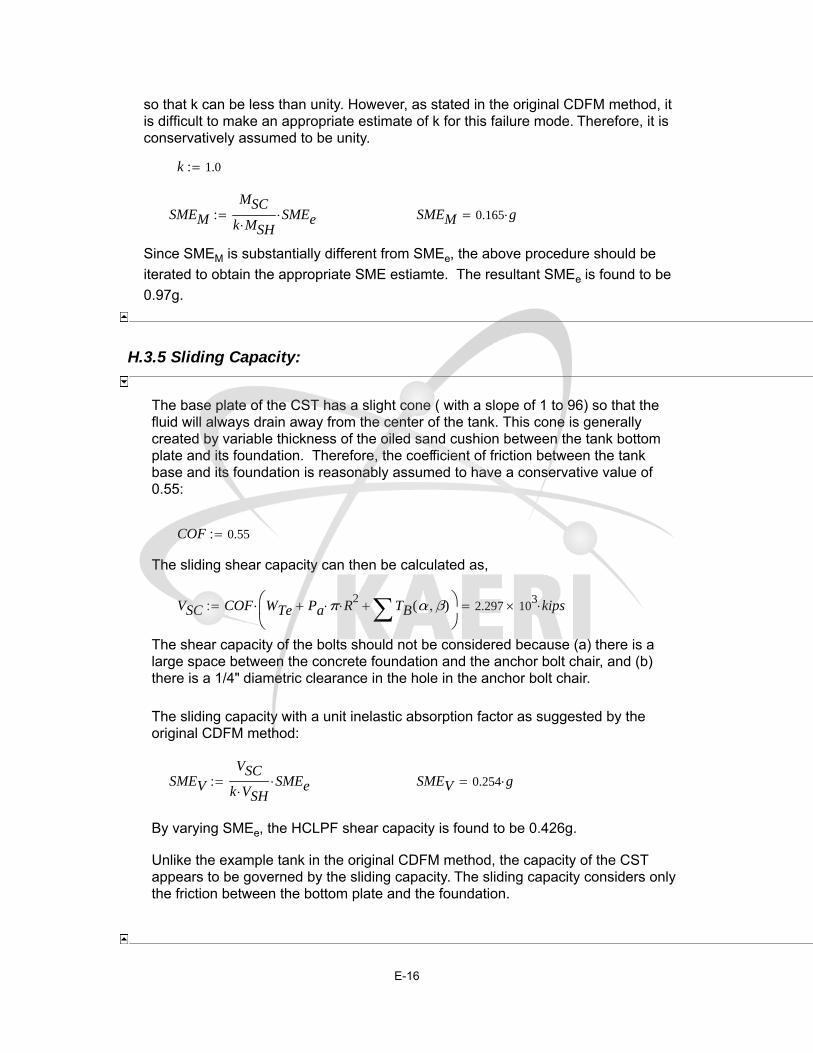
so that k can be less than unity. However, as stated in the original CDFM method, itis difficult to make an appropriate estimate of k for this failure mode. Therefore, it isconservatively assumed to be unity.

k 1.0

SMEM

MSC

k MSHSMEe SMEM 0.165 g

Since SMEM is substantially different from SMEe, the above procedure should be

iterated to obtain the appropriate SME estiamte. The resultant SMEe is found to be

0.97g.

H.3.5 Sliding Capacity:

The base plate of the CST has a slight cone ( with a slope of 1 to 96) so that thefluid will always drain away from the center of the tank. This cone is generallycreated by variable thickness of the oiled sand cushion between the tank bottomplate and its foundation. Therefore, the coefficient of friction between the tankbase and its foundation is reasonably assumed to have a conservative value of0.55:

COF 0.55

The sliding shear capacity can then be calculated as,

VSC COF WTe Pa π R2 TB α β( )

2.297 103 kips

The shear capacity of the bolts should not be considered because (a) there is alarge space between the concrete foundation and the anchor bolt chair, and (b)there is a 1/4" diametric clearance in the hole in the anchor bolt chair.

The sliding capacity with a unit inelastic absorption factor as suggested by theoriginal CDFM method:

SMEV

VSC

k VSHSMEe SMEV 0.254 g

By varying SMEe, the HCLPF shear capacity is found to be 0.426g.

Unlike the example tank in the original CDFM method, the capacity of the CSTappears to be governed by the sliding capacity. The sliding capacity considers onlythe friction between the bottom plate and the foundation.

E-16

H.3.6 Fluid Pressure Capacity:

The inelastic energy absorption seismic response reduction factor kμ is suggested

to be 0.8 for HCLPF capacity evaluation:

ku 0.8

For the CDFM hoop membrane stress capacity, it is recommended that the ASMEseismic design limit of 2 SM for primary stress should be used, which is 37.5 ksi for

SA240-type 304 stainless steel:

σa 37.5ksi

The pressure capacity, PCA, at the bottom of the tank shell (the CST has a uniform

shell thickness), can be estimated to be:

PCA t( )σa t

R

PCA tS 78.044 psi

The maximum seismic induced hydrodynamic pressures PSM and the hydrostatic

pressure PST at the bottom of the tank shell are:

PSM H( ) 4.283 104 Pa

PST H( ) 1.12 105 Pa

The HCLPF fluid pressure capacity SMEP can be determined as:

SMEp

PCA tS PST H( )

ku PSM H( )SMEe 2.052 g

By varying SMEe, the HCLPF fluid pressure capacity can be found to be 2.191 g,which does not govern. This agrees with seismic experience that the fluidpressure capacity seldom appears to govern the seismic capacity for normal flatbottomed steel tanks with butt-welded side plates.

Summary of SME capacities:

SMEM 0.165 g

SMEV 0.254 g

E-17

SMEp 2.052 g

SMEcr min SMEM SMEV SMEp 0.165 g

SMEe 0.165 g

if SMEcr SMEM= "Moment" if SMEcr SMEV= "Shear" "Fluid Pressure" "Moment"

year 80

crack 0.624 mm

Summary of results:

Years: 0 5 10 15 20 25 30 35 40cr (mm): 0. 0.039 0.078 0.117 0.156 0.194 0.234 0.273 0.312SME: 0.426 0.426 0.426 0.426 0.426 0.424 0.416 0.399 0.371SMEM: 1.140 1.140 1.140 1.140 1.140 1.127 1.045 0.900 0.704SMEV: 0.426 0.426 0.426 0.426 0.426 0.424 0.416 0.399 0.371SMEP: 2.052 2.052 2.052 2.052 2.052 2.052 2.052 2.052 2.052Mode: Shear Shear Shear Shear Shear Shear Shear Shear Shear

Years: 45 50 55 60 65 70 75 80cr (mm): 0.351 0.390 0.429 0.468 0.507 0.546 0.585 0.624SME: 0.330 0.240 0.165 0.165 0.165 0.165 0.165 0.165SMEM: 0.472 0.240 0.165 0.165 0.165 0.165 0.165 0.165SMEV: 0.330 0.282 0.254 0.254 0.254 0.254 0.254 0.254SMEP: 2.052 2.052 2.052 2.052 2.052 2.052 2.052 2.052Mode: Shear Moment Moment Moment Moment Moment Moment Moment

H.3.7 Consideration of Other Capacities:

(1) Slosh height for roof damage: note that even with a SMEe = 0.334 g (the initial

guess), the slosh height is about 4.8 ft. With the HCLPF shear capacity of

SMEe=0.555 g, the sloshing height can be about 7.9 ft, which is close to the total

height of the head (8.7', as approximated in the beginning part of this calculation).

hs 2.36 ft SMEe 0.165 g

The increase of sloshing height is not significant as SMEe increases from 0.334 gto 0.555 g. In addition, as pointed out in the original CDFM method, even if roofdamage might be expected, such damage usually does not impair the ability of thetank to contain fluid.

(2) The CST is assumed to sit on rock/very stiff soil; therefore, soil-tankfoundation interaction is not considered.

(3) Piping failure or failure of nozzles may lead to loss of fluid in the tank, andmore importantly, may impair the normal function of the condensation system. Asreported in the original CDFM method, a significant fraction of the cases ofseismic induced loss of tank contents have been due to piping/nozzle failuresbecause of poor detailing. The CDFM method also stated that a SME evaluationof piping/nozzle failure is only necessary when poor seismic detailing is found in

E-18

the involved piping attached to the tank. This analysis assumes that the subjectCST is appropriately detailed, i.e. the piping and nozzle directly attached to thetank are properly designed and constructed so that sufficient piping flexibility canbe achieved to accommodate large relative seismic anchor movements.

(4) The influence of the building in between the two CSTs on the SME areassessed in the following. The gap between the auxiliary building and the CSTsat the roof level is filled with elastomeric sealant.

The maximum tank shell uplift distortion is found to be 0.026 in, whichcorresponds to a neutral axis angle β of 2.29161 rad. Since the horizontal plane atthe anchor bolt chair is assumed to remain plane and all distortion is assumed tooccur below this level, the rotation angle around the neutral axis can be estimatedto be:

Rotationδe0

R 1 cos β( )( )2.015 10

3

β 3.004 cos β( ) 0.991

The maximum horizontal displacement at the roof of the auxiliary building, whichis at an elevation of 114' 9" (Parapet elevation, compared to the tank floorelevation of 101' 9"), can be estimated to be:

Rotation 13 ft 0.314 in

This horizontal displacement is much less than the width of the seismic separationjoint at the roof elevation, which is 3 in. Therefore, the influence of the auxiliarybuilding to the two CSTs is considered minimal.

The Fragility of CST

Summary of results:

Years: 0 5 10 15 20 25 30 35 40cr (mm): 0. 0.039 0.078 0.117 0.156 0.194 0.234 0.273 0.312SME: 0.426 0.426 0.426 0.426 0.426 0.424 0.416 0.399 0.371SMEM: 1.140 1.140 1.140 1.140 1.140 1.127 1.045 0.900 0.704SMEV: 0.426 0.426 0.426 0.426 0.426 0.424 0.416 0.399 0.371SMEP: 2.052 2.052 2.052 2.052 2.052 2.052 2.052 2.052 2.052Mode: Shear Shear Shear Shear Shear Shear Shear Shear Shear

Years: 45 50 55 60 65 70 75 80cr (mm): 0.351 0.390 0.429 0.468 0.507 0.546 0.585 0.624SME: 0.330 0.240 0.165 0.165 0.165 0.165 0.165 0.165SMEM: 0.472 0.240 0.165 0.165 0.165 0.165 0.165 0.165SMEV: 0.330 0.282 0.254 0.254 0.254 0.254 0.254 0.254SMEP: 2.052 2.052 2.052 2.052 2.052 2.052 2.052 2.052Mode: Shear Moment Moment Moment Moment Moment Moment Moment

E-19

SMEHCLPF 0.426 0.426 0.426 0.426 0.426 0.424 0.416 0.399 0.371 0.330 0.240(

SMEM 1.140 1.140 1.140 1.140 1.140 1.127 1.045 0.900 0.704 0.472 0.240 0.16(

SMEV 0.426 0.426 0.426 0.426 0.426 0.424 0.416 0.399 0.371 0.330 0.282 0.25(

SMEP 2.052 2.052 2.052 2.052 2.052 2.052 2.052 2.052 2.052 2.052 2.052 2.052(

It should be emphasized that the HCLPF SME capacity assumes the RegulatoryGuide 1.60 spectra anchored to the HCLPF SME PGA.

To determine the seismic fragility of the CST tank, one needs to convert theHCLPF SME PGA to median SME PGA. This conversion requires the estimate ofboth aleatory and epistemic uncertainties (βR and βU). The Fragility Method, also

presented along with the original CDFM method, estimates the aleatory andepistemic uncertainties to be 0.2 and 0.27, respectively. These uncertainties arenearly identical to those reported by Choun, et al [2008]. The SME median SMEm

can then be estimated as well.

i 0 1 16

βR 0.2

βU 0.27

βC βR2

βU2 0.336

Hm exp 1.645 βR βU 2.167

SMEmiSMEHCLPFi

Hm

SMEMmiSMEMi

Hm

SMEVmiSMEVi

Hm

SMEPmiSMEPi

Hm

E-20

F Q a( ) cnorm

lna g

SMEm

βU qnorm Q 0 1( )

βR

Fmean a( ) cnorm

lna g

SMEm

βC

sa 0.05 0.1 3

0 1 2 30

0.2

0.4

0.6

0.8

1

0 - 20 Years25 Years30 Years35 Years40 Years45 Years50 Years (Moment)55-80 Years (Moment)

CST Fragility

PGA (g)

Fra

gili

ty

yeari i 5

E-21

0 5 10 15 20 25 30 35 40 45 50 55 60 65 70 75 800

0.5

1

1.5

2

2.5

HCLPF CapacityOverturning Moment CapacitySliding CapacityFluid Pressure Capacity

Time (year)

HC

LP

F F

ragi

lity

Cap

acit

y (g

)

E-22

0 5 10 15 20 25 30 35 40 45 50 55 60 65 70 75 800

1

2

3

4

5

Median CapacityOverturning Moment CapacitySliding CapacityFluid Pressure Capacity

Time (year)

Med

ian

Fra

gili

ty C

apac

ity

(g)

E-23

0 0.165 0.165 0.165 0.165 0.165 0.165 )T

g

65 0.165 0.165 0.165 0.165 0.165 )T

g

54 0.254 0.254 0.254 0.254 0.254 )T

g

2 2.052 2.052 2.052 2.052 2.052 )T

g

E-24

Appendix F FRAGILITY ANALYSIS OF THE CST WITH MULTIPLE DEGRADATIONS

KAERI Year 3 Task

Fragility Analysis of Condensate Storage Tank

- Combining Degradation Cases A, B, and C

This calculation combines degradation cases (A) stainless steel tank shell, (B) anchorbolts, and (C-2) anchorage concrete cracking. In this evaluation, all threedegradations are assumed to occur simultaneously and to be perfectly correlated.

year 65

SMEe 0.032g

Degradation Case A: Stainless Steel Tank Shell

scc_rate 7.494 103 in

tshell_degraded5

8in scc_rate year 0.138 in

Degradation Case B: Anchor Bolts

C 70.6

α 0.79

X t( ) C tα μm

Dbolt_degraded 2.5in 2 X year( ) 2.34962 in

Degradation Case C: Anchorage concrete cracking - BNL model

crack 0.0078 year mm 0.02 in

H.1 Introduction

KAERI indicated that the seismic DBE in Korea follows the NRC Reg. Guide 1.60design spectrum shape but with a PGA level scaled down to 0.2 g. An initial HCLPFcapacity was assumed to be 1.67 times of 0.2 g. However, since the Mathcad

F-1

sheets in this appendix solve the various equations iteratively by manually settingSMEe to different values, the above SMEe value of 0.032 g represents the converged

solution for the degradation level of the combined degradations at 65 years.

H.2 Response EvaluationSame as Appendix A, Section H.2.

H.3 Capacity Assessment

The seismic overturning moment capacity of the CST at its base, MSC, depends

on the axial compressive buckling capacity of the tank shell Cm, the tensile

hold-down capacity of the anchor bolts including their anchorage and attachmentto the tank TBC, and the hold-down capacity of the fluid pressure acting on the

tank base plate Te.

Although unlikely for larger radius tanks, the tank SME capacity is sometimesgoverned by the sliding shear capacity at the tank base, VSC. Even though it does

not appear that any butt welded steel tank has ever failed due to seismic inducedmembrane hoop stresses due to combined hydrostatic and hydrodynamic fluidpressures, the SME capacity of this failure mode, PCA, should also be checked.

Additional assessment of the seismic capacity may include the possibility andconsequence of the fluid sloshing against the tank roof, foundation failure for soilsites, and possibility of failure of piping or their attachment to the tank.

H.3.1 Compressive Buckling Capacity of the Tank Shell:

The most likely buckling for tanks is the "elephant-foot" buckling near the base ofthe tank shell. The "elephant-foot" buckling is a combined effect of hoop tension,axial (vertical) compression, and restriction of radial deformation of the tank shellby the base plate. "Elephant-foot" buckling does not necessarily lead to failure of atank (e.g., leakage). However, there is no simple capability evaluation method thatcan predict tank performance after the development of "elephant-foot" buckling.Therefore, for a CDFM SME capacity of tanks, the onset of "elephant-foot"buckling will be judged to represent the limit to the compressive buckling capacityof the tank shell. The onset of "elephant-foot" buckling can be estimated usingelastic-plastic collapse theory as presented in the following:

The sidewall thickness near the shell base: ts tshell_degraded 0.138 in

F-2

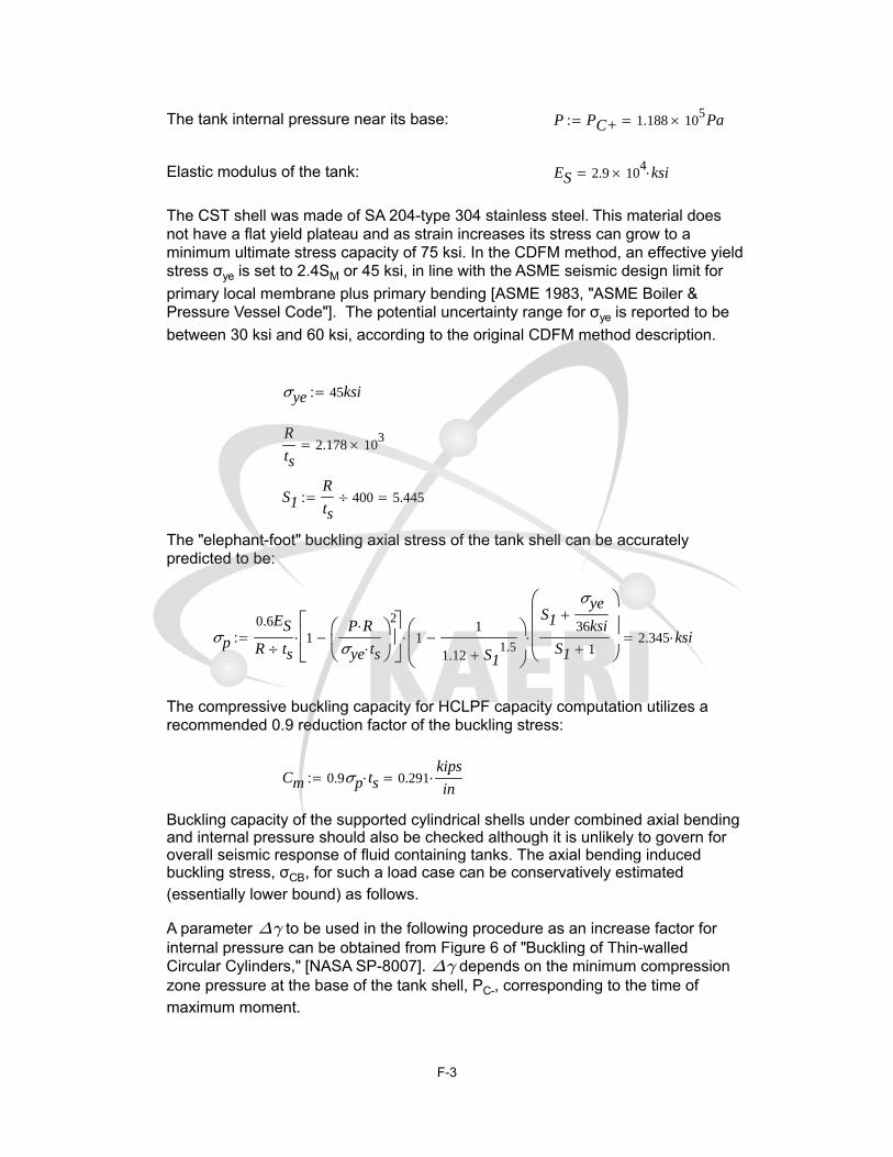
The tank internal pressure near its base: P PC+ 1.188 105 Pa

Elastic modulus of the tank: ES 2.9 104 ksi

The CST shell was made of SA 204-type 304 stainless steel. This material doesnot have a flat yield plateau and as strain increases its stress can grow to aminimum ultimate stress capacity of 75 ksi. In the CDFM method, an effective yieldstress σye is set to 2.4SM or 45 ksi, in line with the ASME seismic design limit for

primary local membrane plus primary bending [ASME 1983, "ASME Boiler &Pressure Vessel Code"]. The potential uncertainty range for σye is reported to be

between 30 ksi and 60 ksi, according to the original CDFM method description.

σye 45ksi

R

ts2.178 10

3

S1R

ts400 5.445

The "elephant-foot" buckling axial stress of the tank shell can be accuratelypredicted to be:

σp

0.6ES

R ts1

P Rσye ts

2

11

1.12 S11.5

S1

σye

36ksi

S1 1

2.345 ksi

The compressive buckling capacity for HCLPF capacity computation utilizes arecommended 0.9 reduction factor of the buckling stress:

Cm 0.9σp ts 0.291kips

in

Buckling capacity of the supported cylindrical shells under combined axial bendingand internal pressure should also be checked although it is unlikely to govern foroverall seismic response of fluid containing tanks. The axial bending inducedbuckling stress, σCB, for such a load case can be conservatively estimated(essentially lower bound) as follows.

A parameter Δγ to be used in the following procedure as an increase factor forinternal pressure can be obtained from Figure 6 of "Buckling of Thin-walledCircular Cylinders," [NASA SP-8007]. Δγ depends on the minimum compressionzone pressure at the base of the tank shell, PC-, corresponding to the time ofmaximum moment.

F-3

Considering the potential range on σye of 30 to 60 ksi, the resultant range on σp is16.572 ksi to 26.702 ksi. Consequently, Cm has a range of 9.322 kips/in to 15.02kips/in.

Since Δγ is to be evaluated based on Figure 6 of NASA SP-8007, this figure isdigitized and defined by the following two vectors, in log scale:

fig6x

1.8197

1.5124

1.395

1.264

1.1422

1.0519

0.94817

0.81296

0.67999

0.52011

0.40087

0.28846

0.18951

0.09283

0.00063874

0.12966

0.22407

0.3071

0.45083

0.57204

0.67305

0.78519

0.86144

0.94893

1.0004

fig6y

1.6448

1.3884

1.3056

1.2088

1.1297

1.0676

1.0058

0.93763

0.86938

0.8017

0.76514

0.7391

0.71278

0.68996

0.66704

0.64849

0.62918

0.62739

0.61269

0.60816

0.60321

0.60915

0.61434

0.6162

0.62796

F-4

Figure 6 of NASA SP-8007: Increase in Axial-CompressiveBuckling-Stress Coefficient of Cylinders due to Internal Pressure

2 1 0 12

1

0

1

log(P/E(R/t_s)^2)

log(

Δγ

)

10linterp fig6x fig6y log 0.166( )( )

0.12004

ipxPC-

ES

R

ts

2

2.678PC-

ES

R

tS

2

0.13

Δγ 10linterp fig6x fig6y log ipx( )( )

0.243

ϕ1

16

R

ts 2.917

γ 1 0.73 1 eϕ 0.309

Note: there is not experimental data for R/t>1500. R

ts2.178 10

3

σCB 0.6γ Δγ( )ES

R ts5.704 ksi

0.9σp 2.11 ksi

F-5

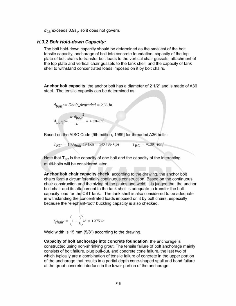
σCB exceeds 0.9sp, so it does not govern.

H.3.2 Bolt Hold-down Capacity:

The bolt hold-down capacity should be determined as the smallest of the bolttensile capacity, anchorage of bolt into concrete foundation, capacity of the topplate of bolt chairs to transfer bolt loads to the vertical chair gussets, attachment ofthe top plate and vertical chair gussets to the tank shell, and the capacity of tankshell to withstand concentrated loads imposed on it by bolt chairs.

Anchor bolt capacity: the anchor bolt has a diameter of 2 1/2" and is made of A36steel. The tensile capacity can be determined as:

dbolt Dbolt_degraded 2.35 in

Abolt

π dbolt2

44.336 in

2

Based on the AISC Code [9th edition, 1989] for threaded A36 bolts:

TBC 1.7Abolt 19.1 ksi 140.788 kips TBC 70.394 tonf

Note that TBC is the capacity of one bolt and the capacity of the interacting

multi-bolts will be considered later.

Anchor bolt chair capacity check: according to the drawing, the anchor boltchairs form a circumferentially continuous construction. Based on the continuouschair construction and the sizing of the plates and weld, it is judged that the anchorbolt chair and its attachment to the tank shell is adequate to transfer the boltcapacity load for the CST tank. The tank shell is also considered to be adequatein withstanding the concentrated loads imposed on it by bolt chairs, especiallybecause the "elephant-foot" buckling capacity is also checked.

tchair 13

8

in 1.375 in

Weld width is 15 mm (5/8") according to the drawing.

Capacity of bolt anchorage into concrete foundation: the anchorage isconstructed using non-shrinking grout. The tensile failure of bolt anchorage mainlyconsists of bolt failure, plug pull-out, and concrete cone failure, the last two ofwhich typically are a combination of tensile failure of concrete in the upper portionof the anchorage that results in a partial depth cone-shaped spall and bond failureat the grout-concrete interface in the lower portion of the anchorage.

F-6

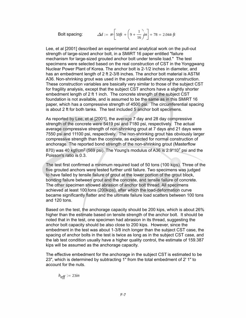
Bolt spacing: Δd π 50ft 91

16

in

78 2.044 ft

Lee, et al [2001] described an experimental and analytical work on the pull-outstrength of large-sized anchor bolt, in a SMiRT 16 paper entitled "failuremechanism for large-sized grouted anchor bolt under tensile load." The testspecimens were selected based on the real construction of CST in the YonggwangNuclear Power Plant of Korea. The anchor bolt is 2-1/2 inches in diameter, andhas an embedment length of 2 ft 2-3/8 inches. The anchor bolt material is ASTMA36. Non-shrinking grout was used in the post-installed anchorage construction.These construction variables are basically very similar to those of the subject CSTfor fragility analysis, except that the subject CST anchors have a slightly shorterembedment length of 2 ft 1 inch. The concrete strength of the subject CSTfoundation is not available, and is assumed to be the same as in this SMiRT 16paper, which has a compressive strength of 4500 psi. The circumferential spacingis about 2 ft for both tanks. The test included 5 anchor bolt specimens.

As reported by Lee, et al [2001], the average 7 day and 28 day compressivestrength of the concrete were 5419 psi and 7180 psi, respectively. The actualaverage compressive strength of non-shrinking grout at 7 days and 21 days were7550 psi and 11100 psi, respectively. The non-shrinking grout has obviously largercompressive strength than the concrete, as expected for normal construction ofanchorage. The reported bond strength of the non-shrinking grout (Masterflow

870) was 40 kgf/cm2 (569 psi). The Young's modulus of A36 is 2.9*107 psi and thePoisson's ratio is 0.3.

The test first confirmed a minimum required load of 50 tons (100 kips). Three of thefive grouted anchors were tested further until failure. Two specimens was judgedto have failed by tensile failure of grout at the lower portion of the grout block,bonding failure between grout and the concrete, and tensile failure of concrete.The other specimen showed abrasion of anchor bolt thread. All specimensachieved at least 100 tons (200kips), after which the load-deformation curvebecame significantly flatter and the ultimate failure load scatters between 100 tonsand 120 tons.

Based on the test, the anchorage capacity should be 200 kips, which is about 26%higher than the estimate based on tensile strength of the anchor bolt. It should benoted that in the test, one specimen had abrasion in its thread, suggesting theanchor bolt capacity should be also close to 200 kips. However, since theembedment in the test was about 1-3/8 inch longer than the subject CST case, thespacing of anchor bolts in the test is twice as long as in the subject CST case, andthe lab test condition usually have a higher quality control, the estimate of 159.387kips will be assumed as the anchorage capacity.

The effective embedment for the anchorage in the subject CST is estimated to be23", which is determined by subtracting 1" from the total embedment of 2' 1" toaccount for the nuts.

heff 23in

F-7

The compressive strength of the concrete is assumed to be 4500 psi, accordingto the above mentioned paper. It should be pointed out that the measuredstrength in the test is higher.

f'c 4500psi

Base case of the anchor bolt strength based on concrete based onNUREG/CR-5434 (Figure 5.20):

k 57

TAC kheff

in

1.5

f'c

psi lbf 421.767 kips

Note that this TAC capacity calculated based on NUREG/CR-5434 is greater than

200 kips as determined in the test as reported in a SMiRT paper by Lee, et al.[2001]. The anchor bolts in the tests reported in NUREG/CR-5434 have adiameter of 3/4" and an embedment of 4", which are much smaller than thoseused in the CST construction. Therefore, the test data in NUREG/CR-5434 willbe used as factors to scale the test data as reported in the paper by Lee, et al.[2001].

fTAC200kips

421.767kips0.474

Strengths for a crack width of 0mm and 0.3 mm can be assumed to be, based onFigure 5.20 of NUREG/CR-5434:

TAC_00 200kips

TAC_03 200kips15.5

57 54.386 kips

TAC as a function of crack width can be established as:

TAC c( ) max TAC_00c

0.3mmTAC_03 TAC_00 0kips

TAC crack( ) 0 kips

TBC 140.788 kips

TBC min TBC TAC crack( ) 0 kips

F-8

H.3.3 Fluid Hold-down Forces:

Schematic Illustration of Tank Bottom Behavior NearTensile Region of Tank Shell [NUREG/CR-5270]

The hold-down force Te increases with increasing fluid pressure P, which

consequently assumes the minimum tension zone fluid press PT-. A number of

other related parameters are also defined below.

P PT- 15.269 psi

ν 0.3tS 0.625 in

Ib

tB3

12 1 ν2 1.917 10

3 in3

ts 0.138 in

tB 7 mmK

ES ts3

12 1 ν2 786.672J

R 25.026 ft

κR

ts3 1 ν

2

0.5

59.988ts 3.502 10

3 m

F-9

MFPR ts

12 1 ν2

1R

H κ

7.995 103 m

2

MFP is a shortcut to MF / PKS

2 K κR

1.237 104 N

The uplift height δe, the hold down tension Te, moment Me, rotation ae, and

maximum positive moment M+ can then be defined as functions of uplift length l:

F l( ) 1KS l

2ES Ib

δe l( )l4

24

1

F l( )

KS l5

72ES IbMFP

l2

6

P

ES Ib

Note: this equation as in theoriginal CDFM method issingular at L= 0 ft. The MFP/Lterm only has a minor effect onTe when L is very small. The

linear approximation in theoriginal CDFM method caneffectively avoid thissingularity.

Te l( ) Pl

2

1

F l( )

KS l2

12ES IbMFP

l

Me l( ) P1

F l( )

KS l

3

12ES IbMFP

The singularity in this equationcan be similarly avoided by thelinear approximation.

M+ l( ) Pl2

8

Me l( )

2P

Me l( )2

2P2

l2

αe l( )P l

312ES Ib

Me l( ) l

2ES Ib

Given

l 0 in

F-10

l2

24

1

F l( )

KS l3

72ES IbMFP

1

6

0=

lmin Find l( ) 6.848 in

Given

lmax 10in

δe lmax( ) 0.165in=

lmax Find lmax( ) 12.46 in

l lmin lmin 0.1in lmax

Linear Approximation:

i 0lmax lmin( )

0.1in

l_veci lmin i 0.1 in

Te0

Te1

lineδe l_vec( )

in

Te l_vec( )in

lbf

82.56

216.98

Te0 if PT- 0psi Te0 0 lbf

in82.56

lbf

in

Te1 if PT- 0psi Te1 0 lbf

in2

216.98lbf

in2

Te_lin δe Te0 Te1 δe

F-11

0 0.05 0.1 0.150

50

100

150

200

Fluid Hold-down vs Uplift Displacement

Maximum Uplift Displacement δe (in)

Hol

d-do

wn

Ten

sion

Te

(lbf

/in)

It should be noted that these equations are derived based on small displacementtheory, and are applicable to the following conditions:

L / R ≤ 0.15. The solution does not consider the stiffening effect of hoop1.behavior on the base plate and consequently conservatively overpredicts thedisplaceδe , as the ratio of L/R becomes larger.

δe / tb ≤ 0.6. As the solution is based on small displacement assumption,2.

which ignores the beneficial influence of the membrane tension in the baseplate to reduce δe for a given Te as in large displacement theory. For

unanchored tanks, Manos (in "earthquake tank-wall stability of unanchoredtanks," Journal of Structural Engineering, Vol 112, No. 8, ASCE, 1986) andHaroun and Badawi (in "nonlinear axisymmetric uplift of circular plates,"Dynamics of Structures, ASCE, 1987) showed that large displacementmembrane theory greatly increases the fluid hold-down force Te and

consequently the uplift δe . Nevertheless, for anchored tanks like the subject

CST, the uplift is not expected to be very large.

Me/Mpb ≤ 0.9; Me/Mps ≤ 0.9; and M+/Mpb ≤ 0.9, where Mpb and Mps are the3.plastic moment capacity of the base plate and shell sidewalls, respectively.These equations are derived from elastic solution, and these conditionsprevent the potential unconservatism.

0.6tB 0.165 in

F-12

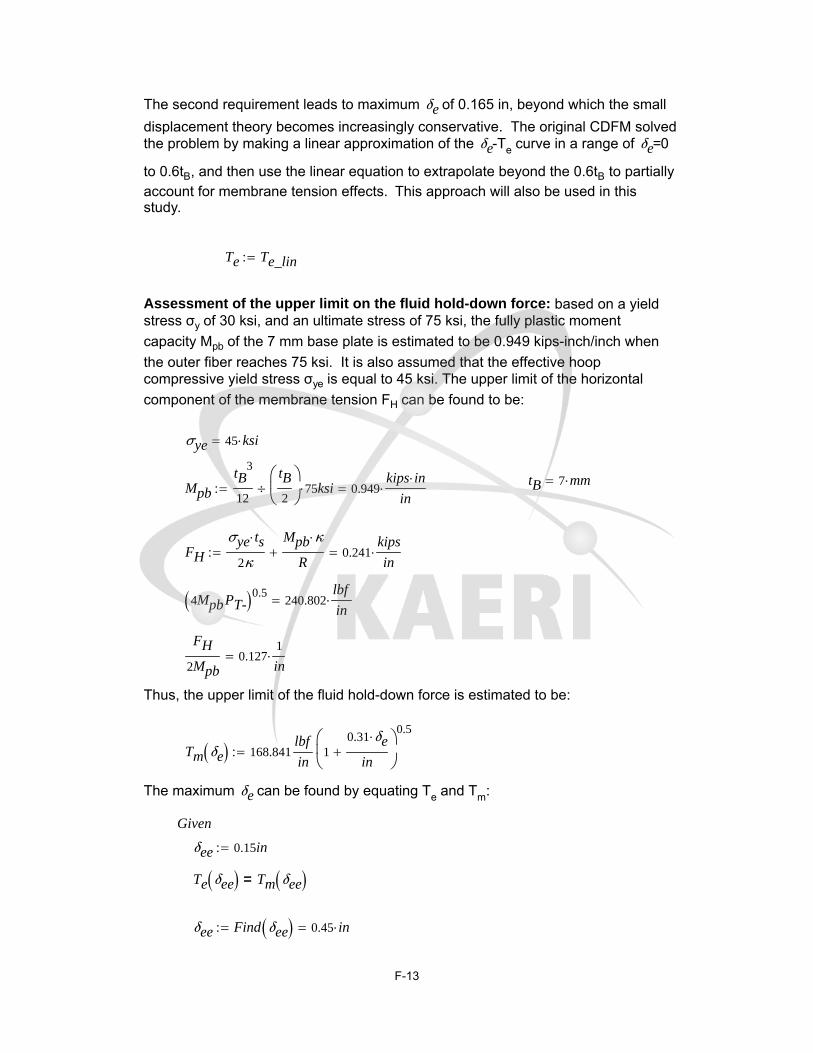
The second requirement leads to maximum δe of 0.165 in, beyond which the small

displacement theory becomes increasingly conservative. The original CDFM solvedthe problem by making a linear approximation of the δe-Te curve in a range of δe=0

to 0.6tB, and then use the linear equation to extrapolate beyond the 0.6tB to partiallyaccount for membrane tension effects. This approach will also be used in thisstudy.

Te Te_lin

Assessment of the upper limit on the fluid hold-down force: based on a yieldstress σy of 30 ksi, and an ultimate stress of 75 ksi, the fully plastic moment

capacity Mpb of the 7 mm base plate is estimated to be 0.949 kips-inch/inch when

the outer fiber reaches 75 ksi. It is also assumed that the effective hoopcompressive yield stress σye is equal to 45 ksi. The upper limit of the horizontal

component of the membrane tension FH can be found to be:

σye 45 ksi

tB 7 mmMpb

tB3

12

tB

2

75 ksi 0.949kips in

in

FH

σye ts

2κ

Mpb κ

R 0.241

kips

in

4MpbPT- 0.5240.802

lbf

in

FH

2Mpb0.127

1

in

Thus, the upper limit of the fluid hold-down force is estimated to be:

Tm δe 168.841lbf

in1

0.31 δe

in

0.5

The maximum δe can be found by equating Te and Tm:

Given

δee 0.15in

Te δee Tm δee =

δee Find δee 0.45 in

F-13

Therefore, the linearized equation for Te should not be extrapolated beyond δee.

Note that linearization is necessary later when developing overturning momentcapacity.

H.3.4 Overturning Moment Capacity:

Vertical Loading on Tank Shell at Base [NUREG/CR-5270]

The overturning moment capacity MSC can be estimated using the compressive

buckling capacity of the tank shell (CB), the anchor bolt hold-down capacity

(TBC), and the relationship between fluid hold-down force and uplift

displacement. The estimation approach in the CDFM method requires several

F-14

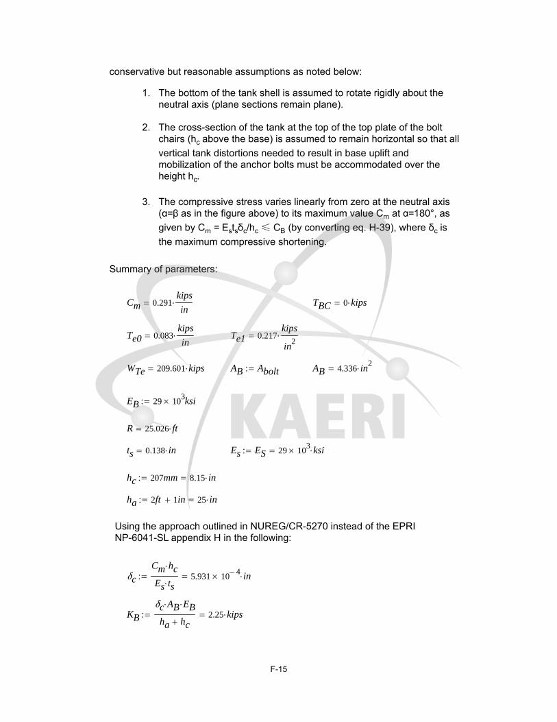
conservative but reasonable assumptions as noted below:

The bottom of the tank shell is assumed to rotate rigidly about the1.neutral axis (plane sections remain plane).

The cross-section of the tank at the top of the top plate of the bolt2.chairs (hc above the base) is assumed to remain horizontal so that all

vertical tank distortions needed to result in base uplift andmobilization of the anchor bolts must be accommodated over theheight hc.

The compressive stress varies linearly from zero at the neutral axis3.(α=β as in the figure above) to its maximum value Cm at α=180°, as

given by Cm = Estsδc/hc ≤ CB (by converting eq. H-39), where δc is

the maximum compressive shortening.

Summary of parameters:

Cm 0.291kips

in TBC 0 kips

Te0 0.083kips

in Te1 0.217

kips

in2

WTe 209.601 kips AB Abolt AB 4.336 in2

EB 29 103ksi

R 25.026 ft

ts 0.138 in Es ES 29 103 ksi

hc 207mm 8.15 in

ha 2ft 1in 25 in

Using the approach outlined in NUREG/CR-5270 instead of the EPRINP-6041-SL appendix H in the following:

δc

Cm hc

Es ts5.931 10

4 in

KB

δc AB EB

ha hc2.25 kips

F-15

ΔTe Te1 δc 1.287 104

kips

in

δea a b( ) δccos a( ) cos b( )

1 cos b( )

Because the bolt pretension TBP is unreliable after a number of years in service, it

is conservatively assumed to be 0.TBP 0kips

The neutral axis angle β can be determined iteratively using the followingprocedure.

Bolt locations: i 0 77

αi2π

78i

Tfunc α β( ) c TBP KBcos α( ) cos β( )

1 cos β( )

c TBC c TBCif

c 0 c 0if

C1 β( )1 cos β( )

sin β( ) π β( )cos β( )

C2 β( )sin β( ) cos β( ) π β

1 cos β( )

C3 β( )sin β( ) β cos β( )

sin β( ) π β( )cos β( )

C4 β( )β sin β( ) cos β( )

1 cos β( )

TB α β( ) Tfunc α β( )

Cf'm α β( )

WTe TB α β( )2R

Te0 β

C1 β( ) ΔTe C3 β( )

Equating Cf'm and Cm to determine β:

func α β( ) Cf'm α β( ) Cm

β root func α β( ) β 0 3.14159( )

F-16

β 0.7382 β180

π 42.296

C'm Cf'm α β( ) 0.291kips

in Cm 0.291

kips

in

Use C'm and β to find the overturning moment capacity MSC:

MSC C'm C2 β( ) R2 TB α β( ) R cos α( )

Te0 R2 2 sin β( ) ΔTe C4 β( ) R

2

MSC 4482.412 kips ft

TB α β( ) 0 kips

The largest bolt elongation (at α=0) should be checked to ensure that theanchorage has the capability:

δe0 δea α0 β 8.874 105 in

Elongation ratio:δe0

ha hc2.677 10

4 %

The maximum elongation ratio is much smaller than 1%, which is recommended inthe original CDFM method for the A307 bolt. One percent is also considered to be anappropriate percentage value for the A36 anchor bolt used in the subject CSTconstruction.

The maximum tank shell uplift distortion δe0 = 0.026 in, which is much less than the

limit of 0.165 in for the small displacement theory to be applicable in developing thefluid hold-down capacity.

Because there are 78 anchor bolts (the example tank in the original CDFM methodhad only 8), the case where α=0 lies midway between bolts need not be checked.

The uncertainty in HCLPF buckling capacity of the tank shell due to the uncertainσye can lead to an MSC as low as 119133.414 kips-ft or as high as 192156.702

kips-ft. It should be noted that unlike in the original CDFM method, MSC is sensitive

to the estimate of Cm.

Inelastic energy absorption reduction factor k can be applied to linearly computedseismic response to obtain the actual overturning moment capacity. The combinedbolt yielding and tank shell buckling failure mode for overturning moment is not brittleso that k can be less than unity. However, as stated in the original CDFM method, itis difficult to make an appropriate estimate of k for this failure mode. Therefore, it isconservatively assumed to be unity.

F-17

k 1.0

SMEM

MSC

k MSHSMEe SMEM 0.033 g

Since SMEM is substantially different from SMEe, the above procedure should be

iterated to obtain the appropriate SME estiamte. The resultant SMEe is found to be

0.97g.

H.3.5 Sliding Capacity:

The base plate of the CST has a slight cone ( with a slope of 1 to 96) so that thefluid will always drain away from the center of the tank. This cone is generallycreated by variable thickness of the oiled sand cushion between the tank bottomplate and its foundation. Therefore, the coefficient of friction between the tankbase and its foundation is reasonably assumed to have a conservative value of0.55:

COF 0.55

The sliding shear capacity can then be calculated as,

VSC COF WTe Pa π R2 TB α β( )

2.581 103 kips

The shear capacity of the bolts should not be considered because (a) there is alarge space between the concrete foundation and the anchor bolt chair, and (b)there is a 1/4" diametric clearance in the hole in the anchor bolt chair.

The sliding capacity with a unit inelastic absorption factor as suggested by theoriginal CDFM method:

SMEV

VSC

k VSHSMEe SMEV 0.285 g

By varying SMEe, the HCLPF shear capacity is found to be 0.555g.

Unlike the example tank in the original CDFM method, the capacity of the CSTappears to be governed by the sliding capacity. The sliding capacity considers onlythe friction between the bottom plate and the foundation.

H.3.6 Fluid Pressure Capacity:

The inelastic energy absorption seismic response reduction factor kμ is suggested

F-18

to be 0.8 for HCLPF capacity evaluation:

ku 0.8

For the CDFM hoop membrane stress capacity, it is recommended that the ASMEseismic design limit of 2 SM for primary stress should be used, which is 37.5 ksi for

SA240-type 304 stainless steel:

σa 37.5ksi

The pressure capacity, PCA, at the bottom of the tank shell (the CST has a uniform

shell thickness), can be estimated to be:

PCA t( )σa t

R

PCA ts 17.218 psi

The maximum seismic induced hydrodynamic pressures PSM and the hydrostatic

pressure PST at the bottom of the tank shell are:

PSM H( ) 8.307 103 Pa

PST H( ) 1.12 105 Pa

The HCLPF fluid pressure capacity SMEP can be determined as:

SMEp

PCA ts PST H( )

ku PSM H( )SMEe 0.032 g

By varying SMEe, the HCLPF fluid pressure capacity can be found to be 2.191 g,

which does not govern. This agrees with seismic experience that the fluidpressure capacity seldom appears to govern the seismic capacity for normal flatbottomed steel tanks with butt-welded side plates.

Summary of SME capacities:

SMEM 0.033 g SMEV 0.285 g SMEp 0.032 g

SMEcr min SMEM SMEV SMEp 0.032 g

SMEe 0.032 g

if SMEcr SMEM= "Moment" if SMEcr SMEV= "Shear" "Fluid Pressure" "Fluid Pressure

year 65 ts 0.138 in dbolt 2.35 in crack 0.507 mm

F-19

Summary of results:

Years: 0 5 10 15 20 25 30 35 40ts (in): 0.625 0.588 0.550 0.513 0.475 0.438 0.400 0.363 0.325 dbolt(in):2.5 2.48 2.466 2.453 2.441 2.429 2.418 2.408 2.398cr(mm): 0 0.039 0.078 0.117 0.156 0.195 0.234 0.273 0.312SME: 0.426 0.408 0.392 0.375 0.358 0.341 0.325 0.309 0.293SMEM: 1.140 1.042 0.946 0.849 0.752 0.657 0.561 0.467 0.372SMEV: 0.426 0.408 0.392 0.375 0.358 0.341 0.325 0.309 0.293SMEP: 2.052 1.896 1.741 1.586 1.430 1.275 1.120 0.964 0.809Mode: Shear Shear Shear Shear Shear Shear Shear Shear Shear

Years: 45 50 55 60 65 70 75 80ts (in): 0.288 0.250 0.213 0.175 0.138dbolt(in):2.388 2.378 2.368 2.359 2.35cr(mm): 0.351 0.390 0.429 0.468 0.507SME: 0.277 0.182 0.068 0.061 0.032 NASMEM: 0.284 0.182 0.068 0.061 0.033SMEV: 0.277 0.279 0.276 0.278 0.285SMEP: 0.654 0.498 0.343 0.187 0.032Mode: Shear Moment Moment Moment Fluid Pressure

H.3.7 Consideration of Other Capacities:

(1) Slosh height for roof damage: note that even with a SMEe = 0.334 g (the initial

guess), the slosh height is about 4.8 ft. With the HCLPF shear capacity of

SMEe=0.555 g, the sloshing height can be about 7.9 ft, which is close to the total

height of the head (8.7', as approximated in the beginning part of this calculation).

hs 0.458 ft SMEe 0.032 g

The increase of sloshing height is not significant as SMEe increases from 0.334 gto 0.555 g. In addition, as pointed out in the original CDFM method, even if roofdamage might be expected, such damage usually does not impair the ability of thetank to contain fluid.

(2) The CST is assumed to sit on rock/very stiff soil; therefore, soil-tankfoundation interaction is not considered.

(3) Piping failure or failure of nozzles may lead to loss of fluid in the tank, andmore importantly, may impair the normal function of the condensation system. Asreported in the original CDFM method, a significant fraction of the cases ofseismic induced loss of tank contents have been due to piping/nozzle failuresbecause of poor detailing. The CDFM method also stated that a SME evaluationof piping/nozzle failure is only necessary when poor seismic detailing is found inthe involved piping attached to the tank. This analysis assumes that the subjectCST is appropriately detailed, i.e. the piping and nozzle directly attached to thetank are properly designed and constructed so that sufficient piping flexibility canbe achieved to accommodate large relative seismic anchor movements.

(4) The influence of the building in between the two CSTs on the SME are

F-20

assessed in the following. The gap between the auxiliary building and the CSTsat the roof level is filled with elastomeric sealant.

The maximum tank shell uplift distortion is found to be 0.026 in, whichcorresponds to a neutral axis angle β of 2.29161 rad. Since the horizontal plane atthe anchor bolt chair is assumed to remain plane and all distortion is assumed tooccur below this level, the rotation angle around the neutral axis can be estimatedto be:

Rotationδe0

R 1 cos β( )( )1.135 10

6

β 0.738 cos β( ) 0.74

The maximum horizontal displacement at the roof of the auxiliary building, whichis at an elevation of 114' 9" (Parapet elevation, compared to the tank floorelevation of 101' 9"), can be estimated to be:

Rotation 13 ft 1.771 104 in

This horizontal displacement is much less than the width of the seismic separationjoint at the roof elevation, which is 3 in. Therefore, the influence of the auxiliarybuilding to the two CSTs is considered minimal.

The Fragility of CST Based on Degraded Conditions

Summary of results:

Years: 0 5 10 15 20 25 30 35 40ts (in): 0.625 0.588 0.550 0.513 0.475 0.438 0.400 0.363 0.325 dbolt(in):2.5 2.48 2.466 2.453 2.441 2.429 2.418 2.408 2.398cr(mm): 0 0.039 0.078 0.117 0.156 0.195 0.234 0.273 0.312SME: 0.426 0.408 0.392 0.375 0.358 0.341 0.325 0.309 0.293SMEM: 1.140 1.042 0.946 0.849 0.752 0.657 0.561 0.467 0.372SMEV: 0.426 0.408 0.392 0.375 0.358 0.341 0.325 0.309 0.293SMEP: 2.052 1.896 1.741 1.586 1.430 1.275 1.120 0.964 0.809Mode: Shear Shear Shear Shear Shear Shear Shear Shear Shear

Years: 45 50 55 60 65 70 75 80ts (in): 0.288 0.250 0.213 0.175 0.138dbolt(in):2.388 2.378 2.368 2.359 2.35cr(mm): 0.351 0.390 0.429 0.468 0.507SME: 0.277 0.182 0.068 0.061 0.032 NASMEM: 0.284 0.182 0.068 0.061 0.033SMEV: 0.277 0.279 0.276 0.278 0.285SMEP: 0.654 0.498 0.343 0.187 0.032Mode: Shear Moment Moment Moment Fluid Pressure

F-21

SMEHCLPF 0.426 0.408 0.392 0.375 0.358 0.341 0.325 0.309 0.293 0.277 0.18(

SMEM 1.140 1.042 0.946 0.849 0.752 0.657 0.561 0.467 0.372 0.284 0.182 0.0(

SMEV 0.426 0.408 0.392 0.375 0.358 0.341 0.325 0.309 0.293 0.277 0.279 0.2(

SMEP 2.052 1.896 1.741 1.586 1.430 1.275 1.120 0.964 0.809 0.654 0.498 0.3(

It should be emphasized that the HCLPF SME capacity assumes the RegulatoryGuide 1.60 spectra anchored to the HCLPF SME PGA.

To determine the seismic fragility of the CST tank, one needs to convert theHCLPF SME PGA to median SME PGA. This conversion requires the estimate ofboth aleatory and epistemic uncertainties (βR and βU). The Fragility Method, also

presented along with the original CDFM method, estimates the aleatory andepistemic uncertainties to be 0.2 and 0.27, respectively. These uncertainties arenearly identical to those reported by Choun, et al [2008]. The SME median SMEm

can then be estimated as well.

i 0 1 13

βR 0.2

βU 0.27

βC βR2

βU2 0.336

Hm exp 1.645 βR βU 2.167

SMEmiSMEHCLPFi

Hm

SMEMmiSMEMi

Hm

SMEVmiSMEVi

Hm

SMEPmiSMEPi

Hm

F-22

F Q a( ) cnorm

lna g

SMEm

βU qnorm Q 0 1( )

βR

Fmean a( ) cnorm

lna g

SMEm

βC

sa 0.05 0.1 3

0 1 2 30

0.2

0.4

0.6

0.8

1

Base Case5 Years10 Years15 Years20 Years25 Years30 Years35 Years40 Years45 Years50 Years55 Years60 Years65 Years

Mean CST Fragilities with Combined Degradations

PGA (g)

Fra

gili

ty

yeari i 5

F-23

0 5 10 15 20 25 30 35 40 45 50 55 60 650

1

2

3

HCLPF CapacityOverturning Moment CapacitySliding CapacityFluid Pressure Capacity

Time (year)

HC

LP

F F

ragi

lity

Cap

acit

y (g

)

0 5 10 15 20 25 30 35 40 45 50 55 60 650

1

2

3

4

5

Median CapacityOverturning Moment CapacitySliding CapacityFluid Pressure Capacity

Time (year)

Med

ian

Fra

gili

ty C

apac

ity

(g)

ii 0 1 12

F-24

yearii ii 5

HCLPFA 0.426 0.409 0.393 0.376 0.360 0.343 0.326 0.310 0.294 0.278 0.218(

HCLPFB 0.426 0.425 0.424 0.423 0.423 0.422 0.422 0.422 0.421 0.42 0.42 0(

HCLPFC 0.426 0.426 0.426 0.426 0.426 0.424 0.416 0.399 0.371 0.330 0.240(

0 5 10 15 20 25 30 35 40 45 50 55 600

0.1

0.2

0.3

0.4

0.5

HCLPF (ABC)HCLPF (A)HCLPF (B)HCLPF (C-2)

Time (Years)

HC

LP

F C

apac

ity

F-25

82 0.068 0.061 0.032 )T

g

068 0.061 0.033 )T

g

276 0.278 0.285 )T

g

43 0.187 0.032 )T

g

F-26

0.152 0.091 )T

g

.419 0.418 )T

g

0.165 0.165 0.165 0.165 0.165 0.165 )T

g

F-27

BIBLIOGRAPHIC INFORMATION SHEET

Performing Org. Report No.

Sponsoring Org. Report No.

Standard Report No. INIS Subject Code

KAERI/TR-4068/2010 BNL-93771-2010

Title / Subtitle Fragility Analysis Methodology for Degraded Structures and Passive Components in Nuclear Power Plants

- Illustrated using a Condensate Storage Tank

Main Author Jinsuo Nie (Brookhaven National Laboratory)

Researcher and Department

Joseph Braverman (Brookhaven National Laboratory) Charles Hofmayer (Brookhaven National Laboratory)

Young-Sun Choun (Korea Atomic Energy Research Institute) Min-Kyu Kim (Korea Atomic Energy Research Institute) In-Kil Choi (Korea Atomic Energy Research Institute)

Publication Place

Upton, USA

Publisher BNL Publication Date

2010. 6

Page 55 p. Ill. & Tab. Yes(O), No ( ) Size 21x29.7cm.

Note

Open Open(O), Closed( ) Report Type Technical Report

Classified Restricted( ), ___Class Document

Sponsoring Org. Contract No.

Abstract (15-20 Lines)

This report describes the seismic fragility capacity for a condensate storage tank with various degradation scenarios. The conservative deterministic failure margin method has been utilized for the undegraded case and has been modified to accommodate the degraded cases. A total of five seismic fragility analysis cases have been described: (1) undegraded case, (2) degraded stainless tank shell, (3) degraded anchor bolts, (4) anchorage concrete cracking, and (5) a perfect correlation of the three degradation scenarios. Insights from these fragility analyses are also presented. An overview of the methods for seismic fragility analysis and generic approaches to incorporate time-dependent degradation models into a fragility analysis is presented. Fundamental concepts of seismic fragility analysis are summarized to facilitate discussions in later sections. The seismic fragility analysis of the undegraded CST, which is assumed to have all of its components in design condition, is described. The subject CST was located in an operating Korean NPP. The baseline fragility capacity of the CST is calculated and the basic procedure of seismic fragility analysis is established. This report presents the results and insights of the seismic fragility analysis of the CST under various postulated degradation scenarios. Subject Keywords (About 10 words)

Seismic Capacity, Fragility, Degradation, Condensate Storage Tank, Tank Shell, Anchor Bolt, Concrete, Cracking, Time-Dependent Model,

Undegraded Case, Degraded Case