Fragile New Economy: The Rise of Intangible Capital and...
50
Fragile New Economy: The Rise of Intangible Capital and Financial Instability * Ye Li † February 28, 2018 Abstract Does the rise of intangible capital create financial instability? Firms hoard liquidity in the form of bank debt (e.g., deposits) for non-pledgeable intangible investments. This liquidity demand pushes down interest rate, giving banks a funding cost advantage, so banks bid up asset prices in booms as they grow. Higher asset prices induce firms to invest more in intangibles and hoard more liquidity, leading to an even lower interest rate and enabling banks to bid up asset prices even further. This paper models corporate savings glut that arises endogenously from the interaction between firms and banks in asset and money markets. The feedback mechanism explains several concurrent phenomena in the run-up to the Great Recession, and how endogenous risk accumulates in booms and materializes into severe and stagnant crises. * I would like to thank my advisors at Columbia University, Patrick Bolton, Tano Santos, and Jos´ e A. Scheinkman. I am grateful to helpful comments from Tobias Adrian, Patrick Bolton, Guojun Chen, Itay Goldstein, Gur Huberman, Christian Julliard, Siyuan Liu, Adriano Rampini, Suresh Sundaresan, and Neng Wang. I am also grateful to conference and seminar participants at Columbia Economics, Columbia Finance, Federal Reserve Bank of New York, Finance Theory Group, and LBS Trans-Atlantic Doctoral Conference. I acknowledge the generous financial support from Macro Financial Modeling Group of Becker Friedman Institute. All errors are mine. † The Ohio State University. E-mail: [email protected] 1
Transcript of Fragile New Economy: The Rise of Intangible Capital and...

Fragile New Economy: The Rise of Intangible Capital
and Financial Instability∗
Ye Li†
February 28, 2018
Abstract
Does the rise of intangible capital create financial instability? Firms hoard liquidity in
the form of bank debt (e.g., deposits) for non-pledgeable intangible investments. This liquidity
demand pushes down interest rate, giving banks a funding cost advantage, so banks bid up asset
prices in booms as they grow. Higher asset prices induce firms to invest more in intangibles
and hoard more liquidity, leading to an even lower interest rate and enabling banks to bid up
asset prices even further. This paper models corporate savings glut that arises endogenously
from the interaction between firms and banks in asset and money markets. The feedback
mechanism explains several concurrent phenomena in the run-up to the Great Recession, and
how endogenous risk accumulates in booms and materializes into severe and stagnant crises.
∗I would like to thank my advisors at Columbia University, Patrick Bolton, Tano Santos, and Jose A. Scheinkman.I am grateful to helpful comments from Tobias Adrian, Patrick Bolton, Guojun Chen, Itay Goldstein, Gur Huberman,Christian Julliard, Siyuan Liu, Adriano Rampini, Suresh Sundaresan, and Neng Wang. I am also grateful to conferenceand seminar participants at Columbia Economics, Columbia Finance, Federal Reserve Bank of New York, FinanceTheory Group, and LBS Trans-Atlantic Doctoral Conference. I acknowledge the generous financial support fromMacro Financial Modeling Group of Becker Friedman Institute. All errors are mine.†The Ohio State University. E-mail: [email protected]
1

1 Introduction
Five trends in the United States have attracted enormous attention in the two decades leading up to
the Great Recession:
(1) The economy was transforming to an intangible-intensive economy. Production of goods
and services increasingly relies on intangible capital, such as brand name, technologies, and or-
ganizational capital. Intangible investment overtook physical investment as the largest source of
growth in the period of 1995-2007 (Corrado and Hulten (2010)).
(2) An increasing share of non-financial corporations’ assets were cash holdings (Bates,
Kahle, and Stulz (2009)). “Cash” is mainly financial intermediaries’ debs, such as bank de-
posits and repurchase agreements (held through money market funds). The rise of corporate cash
holdings is largely due to a growing R&D-intensive sector (Falato and Sim (2014); Begenau and
Palazzo (2015); Pinkowitz, Stulz, and Williamson (2015); Graham and Leary (2015)).
(3) Assets held by the financial sector increased dramatically (Adrian and Shin (2010a);
Gorton, Lewellen, and Metrick (2012); Greenwood and Scharfstein (2013)). Schularick and Taylor
(2012) find that in advanced economies, bank loan-to-GDP ratio doubled in the last two decades.
The growth of financial sector was largely financed by issuing money-like debt securities (Adrian
and Shin (2010b); Gorton (2010); Gorton and Metrick (2012); Pozsar (2014)).
(4) Interest rate declined steadily.
(5) The prices of risky assets increased across asset classes.
Despite extensive debates on the causes and implications of these phenomena, there are few
theories that analyze them jointly. Motivated by Fact (1), I build a continuous-time model of
macroeconomy that highlights the illiquidity of intangible capital and offers a coherent account of
Fact (2) to (5). Moreover, the model reveals a new mechanism of endogenous risk accumulation
that helps understand recent findings in a surging empirical literature: a longer period of bank
expansion precedes a more severe banking and economic crisis (Jorda, Schularick, and Taylor
(2013); Baron and Xiong (2016)). At the center of the mechanism are firms’ needs to hoard money
for future investments and banks’ role as inside money creators.1
1The term, inside money, is borrowed from Gurley and Shaw (1960). From the private sector’s perspective, gold,
1

The model is built upon a simple narrative. The increasing reliance on intangible capital in
the production sector implies a shrinkage of pledgeable assets (physical capital, such as properties,
plants, and equipments). As a result, producers hoard more cash in anticipation of liquidity needs
(e.g., R&D). Cash takes the form of intermediaries’ short-term debts, such as deposits, which
are directly used as means of payment, and close substitutes (e.g., repurchase agreements held
through money market funds). Corporate money demand feeds leverage to the financial sector, so
intermediaries acquire more assets and push up asset prices. The rising corporate money demand
also pushes down interest rates, i.e., yields or expected returns on holdings of money (e.g., deposit
rate) or substitutes (e.g., asset-backed commercial paper rate).
The model has two types of agents, bankers and entrepreneurs. They consume generic goods
produced by firms using tangible and intangible capital. Each entrepreneur manages one firm.
Tangible capital is perfectly liquid in the sense that all of its cash flows are pledgeable and any
claims on them can be traded in secondary markets. To simplify the exposition, it is assumed that
a firm’s tangible capital is traded without any friction between the entrepreneur and bankers. We
can think of tangible capital as inventory, equipments, and real estate. In reality, such assets may
not be traded directly, but securities backed by them as collateral are traded actively. The market of
tangible capital captures such liquidity. Intangible capital is illiquid, representing human capital,
organizational capital, and certain proprietary technologies that are inalienable.
Entrepreneurs choose consumption and tangible capital holdings, and receive goods pro-
duced by their intangible capital. Capital depreciates stochastically, loading on a Brownian shock,
which is the only source of aggregate risk in this economy. Entrepreneurs also face idiosyncratic
liquidity shocks whose arrival follows a Poisson process. When hit by this shock, a firm loses
all capital, but the entrepreneur is endowed with a technology that transforms goods into a fixed
mixture of new tangible and intangible capital. This mixture reflects the necessity of having both
types of capital for firms’ production. New tangible capital can be pledged for external funds,
but intangible capital is illiquid. Therefore, intangible investment requires entrepreneur to hold a
liquidity buffer. Entrepreneurs hold liquidity in the form of bank deposits (short-term safe debt) so
fiat money, or government securities are in positive supply (“outside money”), while as bank liabilities, deposits are inzero net supply (“inside money”). See Lagos (2008) for a brief review of the related literature.
2
that when the liquidity shock hits, they may use deposits to buy goods as investment inputs.
Banks hold a diversified portfolio of different firms’ tangible capital, and issue deposits
(“inside money”) that earn a liquidity premium from entrepreneurs because they serve as a hedge
against liquidity shocks. Banks add value by issuing deposits, the liquid store of value that en-
trepreneurs need to hold for intangible investments. This stands in contrast with the current lit-
erature that emphasize the asset side of bank balance sheet – banks are important because they
extend credit. The model shares one feature with other macro-finance models, that is banks’ equity
issuance constraint. Specifically, banks cannot raise equity in the model. This is a simple method
to condition the equilibrium dynamics on banks’ balance-sheet capacity, so that we can discuss the
implications of intangible capital, and the associated liquidity demand, on financial crises.
This setup helps explain the fact (2) to (5) listed in the beginning of this paper, and reveal a
feedback mechanism that is anchored at the illiquidity of intangible capital and generates amplified
boom-bust cycles. Consider a sequence of positive shocks. Bankers’ wealth (equity) increases, and
they acquire more tangible capital financed by issuing deposits. Because the liquidity premium on
deposits lowers bankers’ debt cost, their required rate of return is lower than that of entrepreneurs.
Therefore, as bankers get richer, they bid up the price of tangible capital. Here, tangible capital is
broadly interpreted as assets in the real world whose cash flow is liquid and from firms’ production.
The rising asset price induces more liquidity holdings by entrepreneurs through two chan-
nels. First, creating new capital is more profitable. Since tangible and intangible capital must be
created simultaneously, to profit from a higher valuation of tangible capital, entrepreneurs must
hold enough liquidity to finance intangible investments. Second, the leverage on entrepreneurs’
liquidity holdings is higher. New tangible capital can be pledged for external financing from banks
at fair price, so through this leverage, entrepreneurs enjoy more surplus from investments when
tangible capital price and the leverage is higher. A stronger liquidity demand of entrepreneurs leads
to a higher liquidity premium, which elevates the price of tangible capital even further by lowering
bankers’ cost of debt and their required return. Finally, any increase of asset price is amplified by
bank leverage and causes bank equity to rise even further. As banks expand their balance sheets,
more deposits are issued and held by entrepreneurs, so more intangible investments are financed.
3

This positive feedback loop links and works through a rising asset price, a declining interest (de-
posit) rate, the expansion of banking sector, and the run-up of corporate liquidity holdings. When
negative shocks hit, the spiral is flipped downward, causing an amplified crisis dynamics.
At the center of this mechanism is an intermediated liquidity premium. Entrepreneurs assign
a liquidity premium to bank deposits, because deposits transfer wealth to the contingencies where
it is needed, working as a hedge against liquidity shocks. This premium lowers the debt cost of
banks and their required rate of return (discount rate), and thereby, translates into a higher price of
tangible capital. This transmission of liquidity premium works through banks’ balance sheet, and it
works better when bankers are wealthier and able to acquire more tangible capital. In other words,
a more well-capitalized banking sector intermediates the liquidity premium more effectively.
The channel of intermediated liquidity premium can cause endogenous risk accumulation in
booms. As previously discussed, a sequence of positive shocks lead to a declining interest rate and
rising liquidity premium by making intangible investments more important. This creates a widen-
ing gap between the required rate of return of bankers and that of entrepreneurs. The difference
the first-best (bankers) and second-best buyers (entrepreneurs) of tangible capital increases, so as
a boom prolongs, the price of tangible capital price becomes increasingly sensitive to the variation
of bankers’ wealth (equity). On the other hand, as bankers become richer, their wealth becomes
more robust to shocks. These two forces create a hump-shaped volatility of tangible capital price.
When the economy starts from a relatively low level of bank equity, asset price volatility rises as
the banking sector grows and the interest rate declines, making the economy increasingly fragile.
The price of tangible capital affects economic growth through entrepreneurs’ incentive to hoard
liquidity, so its volatility has strong impact on the long-run welfare.
The continuous-time framework allows a convenient characterization of the long-run be-
havior of the economy. Specifically, the stationary density is shown together with its cumulative
probability function. Crises are rare, but severe due to the feedback mechanism. Moreover, crises
are stagnant. When a sequence of negative shocks knock the economy into recessions, banks are
undercapitalized and the price of tangible capital is depressed, which discourages entrepreneurs
from investment and liquidity hoarding. As a result, the liquidity premium declines, and banks
4

face higher cost of debt and lower return on equity. Therefore, to climb out of crises, bankers only
accumulate wealth very slowly. The expected time to recovery is shown, and under the benchmark
calibration, it takes almost ten years for the economy to grow out of recessionary states.
The last exercise of this paper is to study the model performances in response to a permanent
increase of the productivity of intangible capital relative to tangible capital. The rise of intangible
capital strengthens the feedback mechanism. Both interest rate and asset price are more sensitive to
shocks. In particular, endogenous risk in the form of asset price volatility doubles. Entrepreneurs
hold more cash in their deposit account, and the economy has a larger banking sector to cater such
stronger demand for liquidity. The economy does grow faster thanks to more liquidity savings
of entrepreneurs, but only with more endogenous risk. Therefore, the model characterizes a risk-
return trade-off in the transition towards a more intangible-intensive economy.
Literature. The structural change towards a new economy that is intangible-intensive has attracted
enormous attention (Corrado and Hulten (2010)). Studies explore the implications of this struc-
tural change in different areas from both theoretical and empirical perspectives, such as Atkeson
and Kehoe (2005) (productivity accounting), McGrattan and Prescott (2010) (current account),
Eisfeldt and Papanikolaou (2014) (asset pricing), Peters and Taylor (2016) (corporate investment),
and Perez-Orive and Caggese (2017) (secular stagnation). This paper looks into the financial sta-
bility implications of intangible capital. There is a large literature on how financial development
affects industrial structure (e.g., Levine (1997); Rajan and Zingales (1998)). However, the reverse
question, how industrial structure affects the financial system, has not yet been well explored. This
paper aims to sheds light on this question.
The model fits into the literature on heterogeneous-agent models. Many frictions manifest
themselves into limits on aggregate risk-sharing between sectors. In this paper, the key friction is
that between bankers and entrepreneurs, the only form of financial contracting is risk-free debt.
Di Tella (2014) notes that perfect risk-sharing shuts down the balance-sheet channel (e.g., Kiy-
otaki and Moore (1997); Bernanke and Gertler (1989)). Many study the macroeconomic and asset
pricing implications of dynamic wealth distribution among heterogeneous agents (e.g., Basak and
Cuoco (1998); Krusell and Smith (1998); Longstaff and Wang (2012); He and Krishnamurthy
5
(2013); Brunnermeier and Sannikov (2014); Moll (2014)). This paper contributes to this literature
by introducing a new type of heterogeneity, that is bankers as money suppliers and entrepreneurs
as money demanders. It gives rise to the channel of intermediated liquidity premium.
A recent literature revives the money view of banking that emphasizes the liabilities of banks
as inside money that lubricates the economy by facilitating trades (Kiyotaki and Moore (2000);
Hart and Zingales (2014); Piazzesi and Schneider (2016); Quadrini (2017)). This paper takes a
step further by modeling bankers as private money suppliers in an entrepreneurial economy that
suffers from capital illiquidity, and shows how this leads to financial instability.2 The theoretical
framework in this paper is inspired by Kiyotaki and Moore (2012) who study the emergence of
bubbly outside money (or fiat money) from capital illiquidity (see also Farhi and Tirole (2012)).
This paper is motivated by the large literature on corporate cash holdings (e.g., Opler et al.
(1999); Bates, Kahle, and Stulz (2009)). The secular increase of nonfinancial firms’ cash holdings
in the last few decades was driven by the R&D-intensive sectors (e.g., Falato and Sim (2014); Be-
genau and Palazzo (2015); Graham and Leary (2015); Pinkowitz, Stulz, and Williamson (2015)).
Physical capital relaxes financial constraints by serving as collateral (Almeida and Campello (2007)).
The structural transformation towards an intangible economy shrinks the collateral pool, leading
to a stronger incentive to hoard liquidity. Corporate treasuries have become a prominent compo-
nent of “institutional cash pools” that lend to the financial sector, particularly through the money
markets (Pozsar (2011)).3
Theoretical models of corporate cash holdings often assume a storage technology (e.g.,
Froot, Scharfstein, and Stein (1993); Bolton, Chen, and Wang (2011); He and Kondor (2016)).
These models characterize a rich environment of corporate decision making, but severs the link
between corporate money demand and the equilibrium interest rate (i.e., the yield on money-like
assets) by assuming a perfectly elastic supply of storage assets. An exception is Holmstrom and
Tirole (1998) and (2001) who take a general equilibrium approach to study whether firms are able
2Safe debt serves as money, which echoes the literature that links the information insensitivity of assets’ payout toassets’ monetary services (Gorton and Pennacchi (1990); Holmstrom (2012); Dang et al. (2014)).
3Several papers have argued that the growth of the shadow banking sector is fueled by the demand of money-likesecurities (e.g., Gorton (2010); Gorton and Metrick (2012); Stein (2012); Pozsar (2014)).
6

to supply the assets they themselves need to hold as liquidity buffer.4 In this paper, firms’ liquidity
demand translates into the demand for bank debt, so that interest rate, asset price, bank leverage,
and corporate cash holdings can be studied in a unified framework
The model predicts that a longer period of boom predicts more severe crisis (asset price
collapse). Schularick and Taylor (2012) find the expansion of bank asset (loans) precedes financial
crises in advanced economies.5 Jorda, Schularick, and Taylor (2013) document a close relationship
between bank credit growth and the severity of subsequent recessions. Related, Baron and Xiong
(2016) find that bank credit expansion predicts increased bank equity crash risk. The existing
theories on endogenous accumulation of risk largely focus on belief distortions (e.g., Gorton and
Ordonez (2014); Moreira and Savov (2017)). This paper emphasizes financial frictions, and the
illiquidity of intangible capital in particular, relating endogenous risk to interest rate dynamics.
The rest of the paper is organized as follows. Section 2 introduces the model and discusses
the mechanisms. Section 3 solves the calibrated model and shows its quantitative performances.
Section 4 concludes. Proofs and solution algorithm are provided in the appendices.
2 Model
2.1 Setup
Consider a continuous-time, infinite-horizon economy with two types of agents, bankers and en-
trepreneurs. Each type has a unit mass of representative agents. We fix a probability space and
an information filtration that satisfy the usual regularity conditions, as defined by Protter (1990).
4Holmstrom and Tirole (2001) explore the impact of corporate liquidity demand on the prices of liquid assets.5In line with Bordo et al. (2001) and Reinhart and Rogoff (2009), Schularick and Taylor (2012) define financial
crises as events during which a country’s banking sector experiences bank runs, sharp increases in default rates accom-panied by large losses of capital that result in public intervention, bankruptcy, or forced merger of financial institutions.Using the information from credit spreads, Krishnamurthy and Muir (2016) are able to achieve a sharper differenti-ation between financial and non-financial crises. They also find that bank credit expansion precedes financial crises.Using both the information from credit spreads and the composition change of corporate bond issuance, Lopez-Salido,Stein, and Zakrajsek (2015) find that when the issuance of high-yield (“junk”) bond outpaced the total bond issuance,and when corporate bond credit spreads are narrow relative to their historical norms, the subsequent real GDP growth,investment, and employment tend to decline.
7
Agents face idiosyncratic Poisson shocks and aggregate Brownian shocks that will be elaborated
later, and make decisions under rational expectation.
Preferences. Agents are risk-neutral and maximize expected utility with discount rate ρ:
E[∫ ∞
t=0
e−ρtdcit
], i ∈ {B,E} . (1)
Throughout this paper, subscripts denote time, and superscripts denote types or sectors. “B” is for
the banking sector and “E” for the entrepreneurial sector. For example, cEt is the representative
entrepreneur’s cumulative consumption up to time t.
Capital and production. Each entrepreneur manages a firm that produces non-durable generic
goods using tangible and intangible capital. In aggregate, the economy has KTt units of tangible
capital and KIt units of intangible capital at time t. One unit of tangible capital produces constant
α units of goods per unit of time. The productivity of intangible capital is α+ φ (where φ > −α).
So from t to t+ dt, the aggregate output is αKTt + (α + φ)KI
t dt.
The two types of capital differ in liquidity. An entrepreneur can sell her firm’s tangible capital
to bankers in a competitive market at price qTt per unit (denominated in goods). After the sale,
entrepreneurs dutifully manage the capital on behalf of banks and deliver the goods produced, so
tangible capital is perfectly liquid in the sense that it is free from any agency friction or asymmetric
information. We may think of tangible capital as inventory, equipments, and houses. In reality,
investors may not trade physical assets directly, but they invest in and trade securities backed by
such assets as collateral. The secondary market captures such liquidity.
In contrast, intangible capital is illiquid. It is attached to the firm and entrepreneur, and
cannot be sold or pledged to outside investors. Intangible capital represents human capital, organi-
zational capital, and certain proprietary technologies that are inalienable.6
Aggregate shock. The only source of aggregate uncertainty in this economy is the Brownian
6The illiquidity of intangible capital may also arise from the difficulty to measure it. Corrado, Hulten, and Sichel(2005) and McGrattan and Prescott (2010) discuss the measurement of technology capital. See Atkeson and Kehoe(2005) and Eisfeldt and Papanikolaou (2014) for organization capital.
8
increment, dZt. As in Brunnermeier and Sannikov (2014), a fraction δdt − σdZt of capital, both
tangible and intangible, are destroyed over dt. We may count capital by its output. For example,
certain number of machines constitute one unit of tangible capital if they are responsible for α units
of goods per unit of time. Intangible capital is counted likewise. Therefore, capital is productive
unit, and the capital destruction shock may accordingly be interpreted as a productivity shock.
Liquidity shock and investment. Entrepreneurs experience liquidity shocks. The arrival of liq-
uidity shock is independent across entrepreneurs (i.e., idiosyncratic ), and follows a Poisson pro-
cess with intensity λ. When hit by a liquidity shock, firms lose all capital, but entrepreneurs are
endowed with a technology to transform goods into new capital instantaneously, and once invest-
ments are made, old capital is restored. Tangible and intangible investments are made simultane-
ously and proportionally: for every 1−θ units of tangible capital, θ units of intangible capital must
be created, vice versa. As a result, the intangible fraction of aggregate capital, KIt /(KIt +KT
t
),
is fixed at θ under the initial condition that KI0/(KI
0 +KT0
)= θ.
θ determines the pledgeability of investment project. Specifically, if an entrepreneur invests
iEt units of goods, it creates κiEt units of capital (constant κ > 0 for investment efficiency), of
which θ fraction is intangible and unpledgeable. The intangible component is a private benefit
for entrepreneurs, while the tangible component can be pledged to banks for financing. Since the
creation of capital is immediate, the entrepreneur repays banks instantaneously with new tangible
capital. The investment scale, iEt , is constrained by the liquid resources:
iEt ≤ κiEt (1− θ)︸ ︷︷ ︸units of new tangible capital
qTt +mEt , (2)
where mEt is the entrepreneur’s liquidity holdings.7 The higher θ is, the more an entrepreneur
relies on mEt to finance investments. When θ = 0, i.e., only tangible investment is made, the
project becomes self-financed as long as κqTt ≥ 1.
Entrepreneurs hold liquidity in the particular form of “bank deposits” that are short-term debt
7Intangible investments rely heavily on firms’ internal liquidity (for example, R&D investments in Hall (1992),Himmelberg and Petersen (1994), and see Hall and Lerner (2009) for a review).
9
of banks with interest rate rt (issued at time t and mature at t + dt). As will be shown later, there
is a unique Markovian equilibrium where banks never default, so their debt is safe. When hit by
liquidity shocks, entrepreneurs use their deposits to purchase goods as investment inputs, so bank
debt effectively serves as means of payment, or “inside money”, and facilitates goods reallocation
towards those who need to invest.8
Let qI denote the value of intangible capital to the risk-neutral entrepreneur. It is simply the
discounted sum of production flows:
qI =α + φ
ρ+ δ, (3)
where the denominator contains the discount rate (ρ) and the expected destruction rate from stochas-
tic depreciation (δ). On the equilibrium path, entrepreneurs’ deposit holdings, mEt , is never zero,
so some investments are always made and old capital is preserved as a result. Therefore, the de-
nominator of qI does not count for the arrival of liquidity shock. Per unit of investment, the new
capital created is worth qIθκ + qTt (1− θ)κ. Going forward, we shall focus on the case where
θ > 0 and κ is sufficiently high so that
qIθκ+ qTt (1− θ)κ > 1,
i.e., investment is a positive-NPV, scalable project. Thus, the entrepreneur wants to maximize the
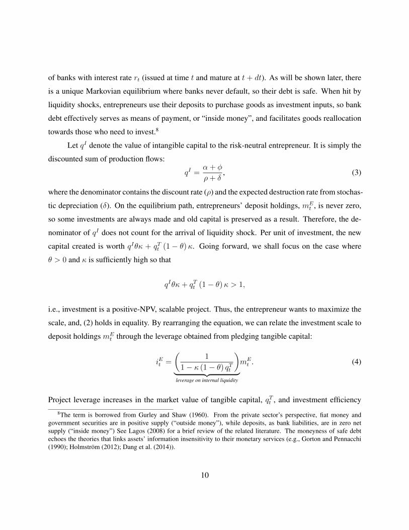
scale, and, (2) holds in equality. By rearranging the equation, we can relate the investment scale to
deposit holdings mEt through the leverage obtained from pledging tangible capital:
iEt =
(1
1− κ (1− θ) qTt
)
︸ ︷︷ ︸leverage on internal liquidity
mEt . (4)
Project leverage increases in the market value of tangible capital, qTt , and investment efficiency
8The term is borrowed from Gurley and Shaw (1960). From the private sector’s perspective, fiat money andgovernment securities are in positive supply (“outside money”), while deposits, as bank liabilities, are in zero netsupply (“inside money”) See Lagos (2008) for a brief review of the related literature. The moneyness of safe debtechoes the theories that links assets’ information insensitivity to their monetary services (e.g., Gorton and Pennacchi(1990); Holmstrom (2012); Dang et al. (2014)).
10
parameter κ, and decreases in the project illiquidity parameter θ.
The fundamental friction in this economy is the illiquidity of intangible capital. If intangible
capital is liquid (pledgeable), the investment project can be self-financed, and thus, entrepreneurs
do not need to carry the liquidity buffer mEt . Equation (4) is a critical element of the model: under
the illiquidity of intangible capital, entrepreneurs’ investment is tied to deposit holdings mEt when
hit by the liquidity shock. Therefore, banks add value to this economy by issuing deposits, a liquid
store of value for entrepreneurs.9 This setup relates to strands of theoretical literature on banks as
inside money creators.10
Banks. Let nBt denote the wealth of a representative banker who invests in firms’ tangible capital
and raises leverage by issuing risk-free debt with interest rate rt. A banker maximizes the risk-
neutral utility in Equation (1) subject to the following budget constraint (flow of funds).
dnBt = xBt nBt dr
Tt + (1− xB)nBt rtdt− dcBt , (5)
where xBt is the fraction of wealth allocated to tangible capital, i.e., the asset-to-equity ratio or bank
leverage, and drTt is the return on tangible capital. In equilibrium, because entrepreneurs hold a
positive amount of bank debt as liquidity buffer, bankers issue debt, and thus, xBt > 1.
To express the return on tangible capital, drTt , we can conjecture that in equilibrium, the
9Holmstrom and Tirole (1998) consider a more general case where firms hold liquidity in the form of other firms’liabilities. Here, the focus is on bank debt as liquidity. There are several reasons why entrepreneurs hold intermediatedliquidity. Entrepreneurs may simply lack the required expertise of asset management. There is a large literature onhouseholds’ limited participation in financial markets (Mankiw and Zeldes (1991); Basak and Cuoco (1998); He andKrishnamurthy (2013)), but firms’ portfolio choice is relatively less studied. Duchin et al. (2017) find firms hold riskysecurities, but what dominate are safe debts issued by intermediaries or governments. Moreover, cross holding isregulated in many countries and industries.
10Kiyotaki and Moore (2000) model bankers as agents with superior ability to make multilateral commitment, i.e.,to pay whoever holds their liabilities, so bank liabilities circulate as means of payment. In a richer setting with limitedcommitment and imperfect record keeping (Kocherlakota (1998)), credit is constrained, so trades must engage in quidpro quo, involving a transaction medium (Kiyotaki and Wright (1989)). Cavalcanti and Wallace (1999) show thatbankers arise as issuers of inside money when their trading history is public knowledge. Ostroy and Starr (1990) andWilliamson and Wright (2010) review the literature of monetary theories. Taking a step further, money creation mayrequire not only a special set of agents (i.e., bankers), but also a particular security design. In Gorton and Pennacchi(1990) and Dang et al. (2014), banks create money by issuing information-insensitive claims (safe debts) that do notsuffer asymmetric information problem in secondary markets.
11

Firm Balance Sheet
Assets Liabilities
Deposits
mEt
Intangible
Capital
Tangible
Capital
Owned by
Entrepreneurs
Owned by banks
kBt , and entre-
preneurs kEt
Bank Balance Sheet
Assets Liabilities
Deposits(xBt − 1
)nBt
Tangible
Capital
kBt = xBt nt/qTt Equity nB
t
Bank asset-to-equity ratio (“leverage”): xBt
Aggregate bank equity: NBt =
∫i∈B n
Bi,tdi
Total output in dt: αKTt + (α + φ)KI
t dt
Figure 1: Model Overview.
market price of tangible capital follows a diffusion process, i.e.,
dqTt = qTt µTt dt+ qTt σ
Tt dt. (6)
Let kBi,t denote the units of tangible capital that banker i holds (kBi,t = xBt nBi,t/q
Tt ). A fraction
δdt− σdZt are destroyed every instant. So, capital holdings depreciate stochastically:
dkBi,t = − (δdt− σdZt) kBi,t. (7)
Using Ito’s lemma, we can solve the return on tangible capital:
drTt =αkBi,tdt
qTt kBi,t
+d(qTt k
Bi,t
)
qTt kBi,t
=
(α
qTt+ µTt − δ + σTt σ
)dt+
(σTt + σ
)dZt. (8)
The term, σTt σ, is from quadratic covariation of Ito’s calculus.
Liquidity creation capacity. Figure 1 summarizes the model structure. Entrepreneurs manage
firms and produce goods using capital for both themselves and bankers who own tangible capital.
There does not exist any agency friction. For one unit of tangible capital owned by bankers,
entrepreneurs dutifully pass a cash flow of α per unit of time. While the cash flow associated
12
tangible capital is fully liquid, the cash flow associated with intangible capital is not, and thus,
entrepreneurs hold deposits issued by banks to finance intangible investments.
Let intervals B = [0, 1] and E = [0, 1] denote the sets of banks and entrepreneurs respec-
tively. NBt =
∫i∈B n
Bi,tdi, is the aggregate net worth of the banking sector, and ME
t =∫i∈Em
Ei,tdi is
entrepreneurs’ aggregate demand for bank deposits. We have the following deposit market clearing
condition:
MEt =
(xBt − 1
)NBt . (9)
Here we utilize the homogeneity of bankers, that is every banker has the same xBt .
Banks add value by issuing deposits that entrepreneurs hold as liquidity buffer. Their capac-
ity to create liquidity depends their wealth (or equity). Following Holmstrom and Tirole (1997),
Bolton and Freixas (2000), Van den Heuvel (2002), Brunnermeier and Sannikov (2014), and Kli-
menko et al. (2016), it is assumed that banks face equity issuance friction. In this model, banks
do not issue equity at all, that is dcBt > 0. By inspecting banks’ budget constraint, Equation (5),
we can see that negative consumption is equivalent to issuing equity.11 This assumption makes
the equilibrium dynamics conditioned upon bankers’ wealth, so the model relates capital intan-
gibility, and the associated liquidity demand of entrepreneurs, to the likelihood and severity of
balance-sheet crisis in the banking sector.
In this economy, the ultimate source of liquidity is tangible capital. While entrepreneurs
cannot diversify away the Poisson shocks that destroy all of their firms’ capital, bankers can pool
tangible capital and use it to back their debt, the inside money. However, to what extent bankers
can provide such diversification or liquidity transformation service depends on their wealth. In
this model, entrepreneurs’ liquidity demand in Holmstrom and Tirole (1998) meets banks’ limited
balance-sheet capacity in Holmstrom and Tirole (1997).12
11Negative consumption is allowed for risk-neutral entrepreneurs (except when the liquidity shock hits), whichis interpreted as dis-utility from additional labor to produce extra goods as in Brunnermeier and Sannikov (2014).Allowing negative consumption fixes entrepreneurs’ required rate of return at ρ and marginal value of wealth at 1, sothat entrepreneurs’ wealth does not add to the dimension of aggregate state variable. Negative consumption serves thesame purpose as assuming large endowments of goods. Because goods are nondurable, entrepreneurs always consumesome to clear the goods market, and thus, their marginal value is pinned down at 1.
12See also, Holmstrom and Tirole (2001), Eisfeldt and Rampini (2009), and Farhi and Tirole (2012) for investment-driven liquidity demand. entrepreneurs’ liquidity demand is likely to be important from an asset pricing perspective.
13
Let Kt = KIt +KT
t denote the total units of capital. It has the following law of motion:
dKt = − (δdt− σdZt)Kt︸ ︷︷ ︸stochastic depreciation
+
[κ
(1
1− κ (1− θ) qTt
)ME
t
]λdt
︸ ︷︷ ︸investment
+ Ktχdt︸ ︷︷ ︸endowments
(10)
The first component is the stochastic depreciation, and the second component is from a measure
λdt of firms who invest an aggregate deposit holdings equal to MEt λdt with a leverage equal to
1/[1− κ (1− θ) qTt
](as in Equation (4)). Finally, the economy is endowed with a flow of new
capital (θKt units are intangible, and (1− θ)Kt units are tangible), evenly distributed among χdt
measure of newly born entrepreneurs. Such endowments capture sources of economic growth
other than the liquidity-constrained investments. To fix the population size, it is assumed that
entrepreneurs exit upon idiosyncratic Poisson arrival with intensity χ and their wealth is evenly
distributed among other entrepreneurs. So, their overall discount rate ρ can be decomposed into
the exit probability χ and a time-discounting rate ρ− χ.
Substituting the deposit market clearing condition (Equation (9)) into Equation (10), we can
relate economic growth directly to bank equity:
dKt
Kt
=
{[κ
(1
1− κ (1− θ) qTt
)(xBt − 1
)(NBt
Kt
)]λ− δ + χ
}
︸ ︷︷ ︸µKt
dt+ σdZt (11)
The expected growth rate of capital, µKt , increases in the ratio of bank equity, NBt , to capital
stock, Kt. When banks are well-capitalized and issue abundant deposits, the economy grows
fast as entrepreneurs are able to invest more out of their liquidity holdings. µKt also increases in
the market price of tangible capital, qTt , which increases the leverage on liquidity holdings and
amplifies the investment scale. Given agents’ risk-neutral preferences, the mean growth rate µKtis directly linked to overall welfare. Therefore, it is clear that under the fundamental friction of
capital intangibility, banks add value by creating inside money that boosts welfare by facilitating
Eisfeldt (2007) show that the liquidity premium of Treasury bills cannot be explained by the liquidity demand fromconsumption smoothing under standard preferences.
14
resources reallocation towards investing agents.
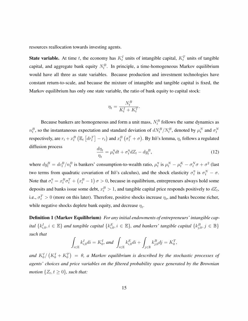
State variable. At time t, the economy has KIt units of intangible capital, KT
t units of tangible
capital, and aggregate bank equity NBt . In principle, a time-homogeneous Markov equilibrium
would have all three as state variables. Because production and investment technologies have
constant return-to-scale, and because the mixture of intangible and tangible capital is fixed, the
Markov equilibrium has only one state variable, the ratio of bank equity to capital stock:
ηt =NBt
KIt +KT
t
.
Because bankers are homogeneous and form a unit mass, NBt follows the same dynamics as
nBt , so the instantaneous expectation and standard deviation of dNBt /N
Bt , denoted by µNt and σNt
respectively, are rt+ xBt(Et[drTt]− rt
)and xBt
(σTt + σ
). By Ito’s lemma, ηt follows a regulated
diffusion process dηtηt
= µηt dt+ σηt dZt − dyBt , (12)
where dyBt = dcBt /nBt is bankers’ consumption-to-wealth ratio, µηt is µNt − µKt − σNt σ + σ2 (last
two terms from quadratic covariation of Ito’s calculus), and the shock elasticity σηt is σNt − σ.
Note that σηt = xBt σTt +
(xBt − 1
)σ > 0, because in equilibrium, entrepreneurs always hold some
deposits and banks issue some debt, xBt > 1, and tangible capital price responds positively to dZt,
i.e., σTt > 0 (more on this later). Therefore, positive shocks increase ηt, and banks become richer,
while negative shocks deplete bank equity, and decrease ηt.
Definition 1 (Markov Equilibrium) For any initial endowments of entrepreneurs’ intangible cap-
ital {kIi,0, i ∈ E} and tangible capital {kEi,0, i ∈ E}, and bankers’ tangible capital {kBj,0, j ∈ B}such that ∫
i∈EkIi,0di = KI
0 , and∫
i∈EkEi,0di+
∫
j∈BkBj,0dj = KT
0 ,
and KI0/(KI
0 +KT0
)= θ, a Markov equilibrium is described by the stochastic processes of
agents’ choices and price variables on the filtered probability space generated by the Brownian
motion {Zt, t ≥ 0}, such that:
15

(i) Agents know and take as given the processes of price variables, such as qTt and rt;
(ii) Entrepreneurs optimally consume, hold deposits, trade tangible capital, and invest;
(iii) Bankers optimally consume, trade tangible capital, and issue deposits;
(iv) Price variables adjust to clear all markets with goods being the numeraire;
(v) All the choice variables and price variables are functions of ηt, so Equation (12) is an
autonomous law of motion that maps any path of shocks {Zs, s ≤ t} to the current state ηt.
2.2 Markov equilibrium
We characterize the Markov equilibrium and will highlight a distinct feedback mechanism that
arises from entrepreneurs’ liquidity demand and puts asset price and interest rate at the center.
Optimal investment and liquidity holdings. Under the assumption that the investment tech-
nology is highly efficient (i.e., κ sufficiently large), entrepreneurs maximize the investment scale
when hit by the liquidity shock. From Equation (4), we know that for one more dollar of liquid-
ity holdings, entrepreneurs can invest 1/[1− κ (1− θ) qTt
]units of goods. And, because exter-
nal funds are raised against tangible capital at fair price, entrepreneurs enjoy all the net present
value (NPV) of investment – for one unit of goods invested, entrepreneurs’ wealth increases by
qIθκ+ qTt (1− θ)κ− 1. Therefore, when the liquidity shock hits, the marginal benefit of liquidity
holdings is precisely the NPV per unit of goods invested multiplied by the leverage on liquidity
holdings:[qIθκ+ qTt (1− θ)κ− 1
]/[1− κ (1− θ) qTt
]. The following proposition states that in
equilibrium, risk-neutral entrepreneurs are willing to accept a deposit rate rt that is lower than
their discount rate ρ, and the wedge ρ− rt, which can be called a liquidity premium, is equal to the
expect marginal benefit of deposit holdings.
16

Proposition 1 (Inside Money Demand) The optimality condition for entrepreneurs’ deposits is
ρ− rt = λ︸︷︷︸probability of liquidity shock
[(qIθ + qTt (1− θ)
)κ− 1
]︸ ︷︷ ︸
NPV per unit of goods invested
(1
1− κ (1− θ) qTt
)
︸ ︷︷ ︸leverage on liquidity holdings
(13)
On the left-hand side is the marginal cost of holding deposits, that is, a lower rate of return
than ρ. On the right-hand side is the marginal benefit, taking into account that a liquidity shock,
and investment opportunities associated with it, arrives with Poisson intensity λ.
Proposition 1 reveals an important link from asset price, qTt , to interest rate, rt, and will
serve as a key building block of a feedback mechanism that reconciles the stylized facts stated in
the introduction and reveals their implications on endogenous risk accumulation. If we consider an
increase in qTt , it translates into an increase of liquidity premium, and thus, a decrease of interest
rate rt, through two channels. First, the NPV per unit of goods invested becomes higher. Second,
the leverage on entrepreneurs’ deposit holdings becomes larger because tangible capital can be
pledged at a higher price for external funds.
Asset price and interest rate. Asset price affects interest rate through entrepreneurs’ liquidity
demand. Standard asset pricing theory suggests that interest rate should also affect asset price
through a typical discount rate channel. This intuition still holds here. To formalize it, we need to
characterize the optimality conditions for entrepreneurs’ and bankers’ tangible capital holdings.
Entrepreneurs’ first-order (indifference) condition is simple and intuitive. The expected re-
turn on tangible capital should not exceed ρ, and when entrepreneurs’ holdings of tangible capital
is positive, it is equal to ρ.α
qTt+ µTt − δ + σTt σ
︸ ︷︷ ︸Et[drTt ]
≤ ρ, (14)
where equality holds when kEt > 0. In contrast to entrepreneurs whose marginal value of wealth is
pinned down to one, the non-negative constraint on bankers’ consumption (i.e., dcBt ≤ 0) suggests
that their marginal value of wealth, denoted by qBt , varies over time in [1,+∞), and dcBt > 0 only
17
when qBt is equal to one. Given the homogeneity nature of bankers’ problem, we can conjecture
that their value function is linear in wealth nBt , and can be written as qBt nBt . In equilibrium, the
marginal value of wealth follows a diffusion process:
dqBtqBt
= µBt dt+ σBt dZt. (15)
The appendix shows that the conjectures of value function and qBt dynamics are confirmed.
σBt measures the shock sensitivity of bankers’ marginal value of wealth, so the instantaneous
covariance between the return on tangible capital drTt and the growth rate of qBt is σBt(σTt + σ
)dt.
An asset with high covariance should have a low expected return, because its realized return is high
precisely when bankers’ marginal value of wealth is high. Therefore, bankers’ required expected
return on tangible capital is equal to rtdt − σBt(σTt + σ
)dt, and we may interpret −σBt as the
price of risk charged by bankers. Because tangible capital is the only asset that bankers hold,
their first-order condition always holds in equality. A formal proof based on bankers’ Hamilton-
Jacobi-Bellman (HJB) equation is provided in the Appendix. The next proposition states bankers’
optimality condition.
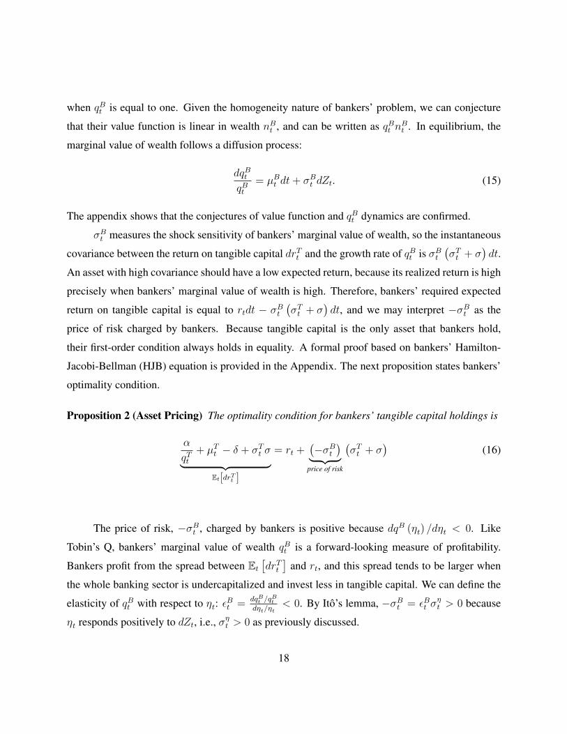
Proposition 2 (Asset Pricing) The optimality condition for bankers’ tangible capital holdings is
α
qTt+ µTt − δ + σTt σ
︸ ︷︷ ︸Et[drTt ]
= rt +(−σBt
)︸ ︷︷ ︸price of risk
(σTt + σ
)(16)
The price of risk, −σBt , charged by bankers is positive because dqB (ηt) /dηt < 0. Like
Tobin’s Q, bankers’ marginal value of wealth qBt is a forward-looking measure of profitability.
Bankers profit from the spread between Et[drTt]
and rt, and this spread tends to be larger when
the whole banking sector is undercapitalized and invest less in tangible capital. We can define the
elasticity of qBt with respect to ηt: εBt =dqBt /q
Bt
dηt/ηt< 0. By Ito’s lemma, −σBt = εBt σ
ηt > 0 because
ηt responds positively to dZt, i.e., σηt > 0 as previously discussed.
18

We can rearrange Equation (16) to express the price of tangible capital as follows
qTt =α
rt − σBt(σTt + σ
)︸ ︷︷ ︸
bankers’ discount rate
− µTt + δ − σTt σ. (17)
Ceteris paribus, an decrease of interest rate rt lowers bankers’ discount rate, and thus, tends to
increase asset price. From Proposition 1 and Proposition 2 arises a feedback mechanism:
Asset price increases → stronger liquidity demand of entrerpreneurs → lower interest rate
→ lower discount rate of bankers → higher asset price ...
At the heart of this mechanism is entrepreneurs’ liquidity demand, which is in turn from the illiq-
uidity of intangible capital. Recall that if intangible capital is pledgeable, the investment project
becomes self-financed, and thus, there is no need for entrepreneurs to carry deposits.
Intermediated liquidity premium. What is still missing in the feedback mechanism is the initial
driver of asset price changes. In a Markov equilibrium with bank equity as the state variable, shocks
affect asset price through their impact on bank equity. The model has a feature that is common
among macro-finance models, that is when intermediaries’ wealth increases, asset price rises (e.g.,
Brunnermeier and Sannikov (2014)). However, the reason behind this feature is different.
In contrast to the existing literature, banks do not add value by having expertise on loans,
such as special monitoring or restructuring abilities (Diamond (1984); Bolton and Freixas (2000)).
Instead, they add value on the liability side of their balance sheets – deposits serve as a liquid store
of value for entrepreneurs, and thus, earn a liquidity premium (rt < ρ). This liquidity premium
gives banks a funding cost advantage in comparison with entrepreneurs. However, due to the equity
issuance constraint (dcBt > 0), bankers are effectively risk-averse and charge a price of risk equal
to −σBt , which puts banks in disadvantage relative to risk-neutral entrepreneurs. In a state of the
world where banks’ equity is very high and their price of risk low, bankers’ funding advantage from
liquidity premium dominates the disadvantage from required risk compensation, so that banks can
19
have a discount rate that is lower than entrepreneurs:
rt − σBt(σTt + σ
)< ρ.
In this case, entrepreneurs do not hold any tangible capital, while banks hold all, i.e., xBt NBt =
qTt KTt . Here, tangible capital should be broadly interpreted as any asset in the real world whose
cash flow is from firms’ production and is liquid (pledgeable).
Inspecting Equation (17), we see that qTt only moves through the discount rate (“DR”) chan-
nel, because the cash flow of tangible capital is fixed at α per unit of time. Note that µTt and σTt ,
the drift and diffusion terms of qTt , are not the fundamental drivers of asset price variation, but
part of the price dynamics itself (as defined in Equation (6)). When bank equity is low and en-
trepreneurs hold tangible capital, the discount rate is fixed at ρ, and we have rt−σBt(σTt + σ
)= ρ
– bankers’ funding cost advantage from the liquidity premium is exactly offset by their disad-
vantage in risk-taking. When bank equity is high and entrepreneurs retreat from tangible capital
market, the discount rate becomes lower than ρ, which boosts qTt . Thus, the states of the world in
this economy are divided into two regions.
In the region where banks are well capitalized, the discount rate for tangible capital is
lowered by an intermediated liquidity premium. Due to the illiquidity of intangible capital, en-
trepreneurs demand a liquid store of value and are willing to pay a liquidity premium, ρ − rt, as
in Holmstrom and Tirole (2001). The ultimate source of liquidity is tangible capital that backs
bank deposits or, in other words, is held by entrepreneurs indirectly through banks’ balance sheets.
Banks’ intermediation capacity depends on their equity, so the transmission of liquidity premium
happens when banks are well capitalized. Driven by the liquidity premium they earn by issuing
deposits, they chase the tangible capital, bidding up its price through a low discount rate.
Intermediated liquidity premium drives qTt even in states of the world with low ηt, where
entrepreneurs still hold some tangible capital, and the discount rate for tangible capital is ρ. Con-
sider a positive shock, dZt > 0. As ηt increases, the economy moves closer to the region where
banks hold all tangible capital and their discount rate is below ρ. Agents’ rational expectation of
a higher qTt going forward is reflected in µTt > 0, the expected price change, which boosts the
20

current tangible capital price as shown in Equation (17). Therefore, qTt always moves positively
with ηt, and its shock elasticity, σTt , is positive.
Intermediated liquidity premium is the key to complete the feedback mechanism. Starting
with an exogenous shock (dZt > 0), we trace out the responses of endogenous variables:
Good shocks → bank equity increases→ asset price increases through DR channel︸ ︷︷ ︸intermediated liquidity premium
→
stronger liquidity demand of entrerpreneurs → higher liquidity premium and lower rt︸ ︷︷ ︸illiquidity of intangible capital & higher investment return
→
lower discount rate of bankers → higher asset price → bank equity increases further︸ ︷︷ ︸typical balance-sheet channel
...
Note that an increase in qTt boosts bank equity through the typical balance-sheet channel because
as the asset value increases, bank equity increases even faster through leverage.
Credit vs. money view of banking. There is a long-standing debate on the function of banks.
Some argue that banks add value because only they are able to finance certain projects (e.g.,
Bernanke (1983)), while others maintain that banks are important because their liabilities, for
instance deposits, serve as a liquid store of value and means of payment, what is often call the
inside money (e.g., Friedman and Schwartz (1963)).13 This paper takes the money view of bank-
ing. Banks add value because entrepreneurs hold deposits as liquidity buffer. This inside money
demand is in line with Woodford (1990) and Holmstrom and Tirole (1998).
However, the model entertains the credit view of banking in the sense that banks finance
entrepreneurs’ investment by extending intraday loans backed by new tangible capital, i.e., sup-
plying the leverage on entrepreneurs’ liquidity holdings. From Equation (4), banks supply more
credit when the price of tangible capital qTt (and entrepreneurs’ financing capacity) is higher. And,13Formalized in Bernanke and Blinder (1992), the credit view on banking has gained much traction recently. In
Brunnermeier and Sannikov (2014), it is embodied by the enhanced productivity when capital is held by banks (“ex-perts”). Other types of intermediation expertise may serve the same purpose of making banks the natural buyers ofcapital and capture the credit view on banking, such as lower risk aversion (Longstaff and Wang (2012)), collateraliza-tion expertise (Rampini and Viswanathan (2015)), unique ability to hold risky assets (He and Krishnamurthy (2013)),unique ability to monitor projects (Diamond (1984) and Holmstrom and Tirole (1997)), and advantage in diversifica-tion (Brunnermeier and Sannikov (2016)). Recent works on the money view of banking includes Hart and Zingales(2014), Quadrini (2017), Piazzesi and Schneider (2016), and Moreira and Savov (2017).
21
qTt is high when banks are well capitalized as previously discussed. Therefore, the model does
exhibit a relation between credit and banks’ balance-sheet capacity, but this relation derives from
the channel of intermediated liquidity premium, i.e., the negative relation between bank equity and
the discount rate in the tangible capital market. Therefore, the first and foremost function of banks
in this economy is still to supply inside money.
Endogenous savings glut and risk accumulation. The model produces endogenous risk accu-
mulation in booms. When we start with a low level of bank equity (low ηt), the instantaneous
volatility of tangible capital price, σTt , increases as ηt and qTt increases.
The rising qTt , through higher the investment NPV and leverage on liquidity holdings, in-
duces an endogenous savings glut on the part of entrepreneurs, which drives down the deposit rate
rt. However, before the banking sector is large enough, entrepreneurs still hold some tangible cap-
ital, so the discount rate is held at ρ. Recall that qTt varies only with the discount rate, so when ηtis low, qTt is relatively insensitive to shocks because the discount rate is likely to stay at ρ. As ηtincreases in booms (in response to positive shocks), the economy moves closer to the region where
banks hold all tangible capital and the discount rate is below ρ, so the likelihood of a discount rate
change rises, making qTt increasingly sensitive to shocks. The instantaneous volatility σTt measures
the shock sensitivity of qTt as shown in Equation (6).
The rising endogenous risk in booms, reflected in asset price volatility, is a distinct feature
of the model. An intuitive way to understand the mechanism is two label bankers as the “first-
best” buyers of tangible capital (as in Shleifer and Vishny (2010)) whose required rate of return is
lower than that of the “second-best” buyers (entrepreneurs) when ηt is high. The discount-rate gap
between these two groups is zero initially, and then widens, as ηt increases and banks dominate the
tangible capital thanks to a rising liquidity premium. A widening difference between the first-best
and second-best buyers makes asset price increasingly sensitive to the wealth of first-best buyers
(bank equity). Even in the region where the discount-rate gap is zero, i.e., rt − σBt(σTt + σ
)= ρ,
the sensitivity of qTt to bank equity increases smoothly as ηt increases, because future discount-rate
gap feeds into the current price volatility through agents’ rational expectation.
Asset price volatility is important from a welfare perspective. As shown in Equation (11),
22
the economic growth rate is directly tied to asset price through the scale of investment (leverage
on entrepreneurs’ liquidity holdings). A high level of asset price enlarges entrepreneurs’ financing
capacity, and a low level reduces it. Therefore, the volatility of asset price translates into the
volatility of economic growth rate, and agents’ long-run welfare.
Stationary distribution and recovery time. To study the long-run behavior of the economy, it is
useful to characterize the stationary probability distribution of the state variable. Another object
of interest is the time to recovery, i.e., how long does it take in expectation for ηt to travel from a
low level with low or even negative economic growth rate to a state with high economic growth
rate. Proposition 3 solves the stationary probability density of ηt and the expected time to reach
η ∈ (0, η] from a low level ηt = η (“recovery time”). Here, endogenous variables are explicitly
written as functions of state variable ηt. Since we study a time-homogeneous Markov equilibrium,
time subscripts are suppressed.
Proposition 3 The stationary probability density of state variable ηt, p(η) can be solved by:
µη (η) p(η)− 1
2
d
dη
(ση (η)2 p(η)
)= 0,
where µη (η) and ση (η) are defined in Equation (12). The expected time to reach η from η, g (η)
can be solved by:1− g′ (η)µη (η)− ση (η)2
2g′′ (η) = 0,
with the boundary conditions g(η)= 0 and g′
(η)= 0.
Solving the equilibrium. In the next section, equilibrium properties of the model are presented
by the calibrated solution. To solve the Markov equilibrium, we can convert agents’ optimality
conditions and market clearing conditions into a system of ordinary differential equations (ODEs).
In particular, bankers’ optimality condition for tangible capital holdings and their HJB equation
form a pair of second-order ODEs for the two forward-looking variables, qB (ηt) and qT (ηt).
Once these two variables are solved, other endogenous variables can be derived as functions of the
level and first derivatives of qB (ηt) and qT (ηt). Details are provided in the Appendix. The next
proposition summarizes the equilibrium solution.
23

Proposition 4 (Markov Equilibrium) There exists a unique Markov equilibrium with state vari-
able ηt that follows an autonomous law of motion in (0, η], where η, the upper bound, is pinned
down by bankers’ optimal consumption. Specifically, we have the boundary conditions:
At η: (1) dqT (ηt)dηt
= 0; (2) qB(η)= 1; (3) dqB(ηt)
dηt= 0;
As ηt approaches zero: (4) limηt→0
dqT (ηt)dηt
= 0; (5) limηt→0
qB (ηt) = +∞.
(1) guarantees that qTt does not jump at the reflecting boundary η (no arbitrage). (2) and (3) are
the value-matching and smooth-pasting conditions for bankers’ consumption choice respectively.
As ηt approaches zero, the likelihood of a discount rate change for tangible capital shrinks to zero,
so qTt becomes insensitive to state variable variation as stated in (4). When banks are extremely
undercapitalized, the their marginal value of equity, or Tobin’s Q, approaches infinity as stated
in (5). Given these boundaries conditions, functions qB (ηt) and qK (ηt) are solved by a pair of
second-order ODEs constructed from bankers’ optimality condition for tangible capital holdings
and their HJB equation. Other variables can be solved as functions of the level and first derivatives
of qB (ηt) and qK (ηt) based on the other optimality and market-clearing conditions.
3 Solution
We now turn to the quantitative analysis of the model, and in particular, how the model generates
the stylized facts summarized in the introduction and how the feedback mechanisms lead to the
accumulation of endogenous risk in booms. The model solution characterizes the full dynamics of
the economy instead of perturbations around the steady state.
3.1 Calibration
One unit of time is set as one year. Entrepreneurs’ time-discounting rate is 6%, roughly in line with
the expected return in the stock and corporate bond markets. Their exit/entry rate is χ = 4%, so
overall, their discount rate ρ is 6%+4% = 10%. The instantaneous mean of stochastic depreciation
rate δ is = 5%. Together with χ = 4%, it generates a long-run mean of µKt , the growth rate of
24
the economy, equal to 1.8%. The long-run mean of a variable is calculated based on the stationary
probability density. The instantaneous volatility of capital depreciation σ is 2%, which is a pivotal
parameter for banks risk-taking and generates a long-run mean of bank leverage equal to 19. The
stochastic depreciation of capital can be broadly interpreted as random failure of production units.
δ and σ are comparable to the time-series mean and standard deviation of delinquency rates on
commercial and industrial loans (source: FRED at Federal Reserve Bank of St. Louis).
On the investment technology, the fraction of inputs that go to intangible investment, θ, is
set to 70%, so the long-run mean of project leverage, defined in Equation (4), is 1.5 in line with
the time-series average of US corporate leverage (source: FRED at Federal Reserve Bank of St.
Louis). Liquidity shock arrives every ten years, so λ = 1/10. The economy has a constant source
of growth from the entry of new entrepreneurs, governed by χ, and a state-dependent source of
growth from liquidity-constrained investments. Therefore, λ is a pivotal parameter for the range of
variation of µKt . Under the current calibration, the economic growth rate µKt varies between −1%to 4% under λ = 1/10. The parameter of investment efficiency, κ, is critical for marginal benefit
of liquidity holdings, so it is set to 3 to generate a long-run cash-to-asset ratio of firms equal to
15%, roughly in line with average cash-to-total asset ratio in the Compustat sample.
A key parameter of the model is φ. It measures the productivity gap between tangible and
intangible capital. Thus, the rise of intangible capital is captured by a high value of φ, meaning that
more output is attributed to intangible capital as documented by Corrado and Hulten (2010). In the
baseline calibration, φ is set to 0.01, which is a 20% productivity advantage of intangible capital
over tangible capital (α = 0.05). The productivity of tangible capital α is set to 0.05, implying that
the long-run mean of qTt /α is 7.5, in line with the EV/EBITDA ratio of tangible industries such as
construction, mining, and materials. In the end of this section, we will discuss how the equilibrium
dynamics change when φ increases, and in particular, the decline of interest rate declines and the
rise of endogenous volatility in response.
25
3.2 Equilibrium dynamics
Endogenous variables are plotted against the ratio of bank equity to aggregate output per year, i.e.,
NBt
αKTt + (α + φ)KI
t
=NBt
[α (1− θ) + (α + φ) θ]Kt
=ηt
α (1− θ) + (α + φ) θ.
Figure 2 reproduces the stylized facts summarized in the introduction. Figure 3 decomposes the
feedback mechanism that puts the intermediated liquidity premium at the center. Figure 4 shows
the accumulation of endogenous risk in booms, and the strength of shock amplification mechanism
of the model. Stationary density and recovery time are shown in Figure 5. Figure 6 compares the
model performances under different levels of φ, and shows that the rise of intangible capital (higher
φ) generates higher economic growth rate, low interest rate, and higher endogenous risk.
The stylized facts. Panel A of Figure 2 plots qTt /α, a price-to-cash flow ratio of tangible capital. In
this economy, tangible capital represents all liquid assets that are traded and pledgeable. Therefore,
the increase of qTt should be interpreted as broad increase of asset prices when the banking sector
expands following positive shocks. Recall that in the model, asset price does not move with cash-
flow news because dividend is fixed at α per unit of time. What drives asset price is the discount
rate, which is fixed at ρ when banks are not large to hold all tangible capital, and below ρ in states
of high ηt due to the intermediated liquidity premium. Asset price increases smoothly in ηt even in
states where ηt is low and the discount rate is equal to ρ, because the future possibility of a discount
rate below ρ is incorporated into the current asset price through agents’ rational expectation.
Panel B of Figure 2 plots the deposit rate rt. As shown in Proposition 1, the rising asset price
translates into an increasing liquidity premium, ρ − rt, through entrepreneurs’ investment-driven
liquidity demand. This model produces an endogenous savings glut in the corporate sector that
drives down the interest rate, and drives up asset price, which in turn feeds into corporate liquidity
hoarding.14 This endogenous mechanism stands in contrast with the existing literature that empha-
sizes exogenous savings glut, for example savings from foreign countries, and its implications on
14Investment need is a key determinant of the cross-sectional variation in corporate cash holdings (e.g., Denis andSibilkov (2010); Duchin (2010)), especially for firms with less collateral (e.g., Almeida and Campello (2007); Li,Whited, and Wu (2016)) and more intensive R&D activities (Falato and Sim (2014)).
26

Figure 2: The Stylized Facts. This figure plots the price-to-dividend ratio of tangible capital (Panel A), deposit ratert (Panel B), the ratio of firms’ liquidity holdings to capital value (Panel C), and the fraction of tangible capital heldby banks (Panel D) against the ratio of aggregate bank equity to output.
interest rate, asset price, and financial fragility (Caballero, Farhi, and Gourinchas (2008); Caballero
and Krishnamurthy (2009); Bolton, Santos, and Scheinkman (2018)).
Panel C of Figure 2 plots the ratio of deposit holdings (“cash”) to firms’ total asset value
qTt KTt +q
IKIt . Following positive shocks, ηt increases and firms’ cash-to-asset ratio rises. The pat-
tern reminisce what we observe in the past two decades in the United States. Many have attributed
the enormous corporate cash holdings to an increasing share of firms whose production heavily
relies on intangible capital (Falato and Sim (2014); Begenau and Palazzo (2015); Pinkowitz, Stulz,
and Williamson (2015); Graham and Leary (2015)). Note that as shown in Figure 1, intangible
capital, tangible capital owned by entrepreneurs, and tangible capital owned by bankers are all
27

incorporated in a firm managed by the corresponding entrepreneur. Bankers’ ownership over tan-
gible capital represents in a very general form their claims on the corporate sector. In line with the
assumption of perfect liquidity of tangible capital, an entrepreneur dutifully delivers the constant
stream of cash flow αdt to banks per unit of tangible capital they own, so there does not exist any
agency friction. In the model, the run-up of corporate cash holdings stops when banks take over the
whole market of liquid assets and any further growth of their equity outpaces asset price increase
and crowds out their debt (deposits).
Panel D of Figure 2 plots the fraction of tangible capital owned by banks. It illustrates the
expansion of banking sector, and reminisces such a trend in data that has attracted tremendous
attention in the literature (Adrian and Shin (2010b); Graham and Leary (2015); Greenwood and
Scharfstein (2013); Schularick and Taylor (2012)). Many drivers behind have been proposed,
and among them, a very prominent one is the incentive of banking sector to earn the liquidity
premium by manufacturing money-like securities (Adrian and Shin (2010a); Gorton (2010); Pozsar
(2014)). This explanation echoes the theme of this paper. Banks add value by supplying liquid store
of value to the entrepreneurial sector, and the endogenous savings glut of the latter feeds cheap
leverage to banks. A feedback mechanism arises, putting the intermediated liquidity premium at
the center and linking all together the increase of asset price, the decline of interest rate, corporate
liquidity hoarding, and banking expansion in a booming economy. Next, this feedback mechanism
is analyzed graphically based on the calibrated solution.
The feedback mechanism. Consider a state of the world where ηt is relatively low, for example,
at 5% bank equity-to-output ratio. Following positive shocks, bank equity increases, and through
the channel of intermediated liquidity premium, the price of tangible capital increases. As shown
in Proposition 1, the impact on entrepreneurs’ incentive to hold liquidity is two-fold. First, when
the liquidity shock arrives, the profit per unit of goods invested becomes higher when qTt is higher.
Second, the leverage of liquidity holdings is higher, because the external financing capacity of the
investment project increases in qTt . Panel A and B of Figure 3 exhibit these dynamics.
As the banking sector grows and the liquidity premium enlarges, banks acquire all the tan-
gible capital when bank equity-to-output ratio reaches around 22%, because now banks’ required
28

Figure 3: The Feedback Mechanism. This figure plots the profit per unit of goods invested (Panel A), the leverageon investing entrepreneurs’ liquidity holdings (Panel B), banks’ discount rate (Panel C), and the expected change oftangible capital price (Panel D) against the ratio of aggregate bank equity to output.
rate of return becomes lower than entrepreneurs’ ρ. In a prolonged boom, qTt keeps rising, driving
up the liquidity premium and driving down the deposit rate rt. As shown in Panel C of Figure 3,
banks’ discount rate declines with rt.
Throughout the process, agents’ expectation of future asset price change µTt keeps rising
(Panel D of Figure 3), because, for example, from a bank equity-to-output ratio of 10% to 20%,
the higher ηt, the closer the economy is to the region where the discount rate for tangible capital
is below ρ. The expectation of low discount rate translates into the expectation of high asset price,
which in turn elevates the current level of asset price as shown in Equation (17).
The positive relation between bank equity and asset price arises from the intermediated liq-
29

uidity premium, and given that, any positive shock triggers a feedback mechanism: asset price
rises, driving up the liquidity premium through both investment profit and entrepreneurs’ leverage
on liquidity; the liquidity premium lowers interest rate, feeding banks with cheap financing and
lowering their discount rate, so asset price increases even further.
Endogenous risk. The dynamics of banks’ discount rate has implications not only on the level of
asset price but also on its volatility. Let us consider that the economy moves from an bank equity-
to-output ratio of 10% to 20% following a sequence of positive shocks in Panel C of Figure 3. In
the process, agents rationally change their belief of the distribution of future discount rate in the
tangible capital market. At the beginning, it is unlikely that the discount rate will move away from
ρ in the near future, because it takes sufficiently large shocks to increase ηt all the way to the cutoff
point of 22% bank equity-to-output ratio. But as we move to the right, ηt approaches the cutoff
point, and thus, the likelihood of a discount rate change increases. As a consequence, asset price
qTt becomes more sensitive to shocks (higher σTt ). This dynamics is shown in Panel B of Figure 4
where the ratio of total volatility of tangible capital return, σTt + σ, to exogenous volatility, σ, is
plotted against bank equity-to-output ratio.
The accumulation of endogenous risk sheds light on the findings that a long period of boom
and banking expansion precedes severe crises (e.g., Jorda, Schularick, and Taylor (2013); Baron
and Xiong (2016)). The existing theories attribute to the accumulation of endogenous risk to
learning (Moreira and Savov (2017)) or the lack of information production (Gorton and Ordonez
(2014)). This paper emphasizes financial friction instead of informational distortions, and more-
over, it offers a model that accounts for several phenomena in the pre-crisis period and links them
to the illiquidity of intangible capital.
The volatility amplification effect is strong. At the peak, the total volatility is almost 3.5
times of the exogenous volatility. Here, σ is defined as the measure of exogenous risk. Without
any feedback mechanism, the return on tangible capital always loads on the aggregate shock dZt
through the stochastic depreciation of capital (Equation (8)). As previously discussed, asset price
moves because of the intermediated money premium. Such movement is captured by σTt . This
endogenous risk arises from agents’ optimal choices under constraints and frictions. Through
30

Figure 4: Endogenous Risk Accumulation and Volatility Trap. This figure plots the shock elasticity of statevariable (Panel A), the ratio of total return volatility to exogenous volatility of tangible capital (Panel B), banks’ priceof risk (Panel C), and the instantaneous expected growth rate of the economy (Panel D) against the ratio of aggregatebank equity to output.
entrepreneurs’ liquidity demand, the illiquidity of intangible capital leads to the endogenous risk
of tangible capital.
In Panel B of Figure 4, endogenous risk rises first and then declines when the banking sector
becomes sufficiently large. The eventual decline can be understood by examining the dynamics of
banks’ discount rate in Panel C of Figure 3. After the cutoff point of 22% bank equity-to-output
ratio, banks’ discount rate declines but the rate of change dies out as the banking sector further
expands. Therefore, asset price becomes increasingly less sensitive to shocks.
Another way to understand the hump-shaped asset price volatility is to decompose σTt . By
Ito’s lemma, σTt = εTt σηt , where εTt is the elasticity of qTt to ηt, i.e., εTt =
dqTt /qTt
dηt/ηt. Another source
31

of the eventual decline of σTt is the gradual stabilization of the state variable itself as it increases
(σηt in Panel A of 4). This decomposition of endogenous risk separates the volatility from state
variable and the sensitivity of asset price qTt to state variable ηt. The latter roughly measures
the dependence of tangible capital price on bank equity. As ηt increases, the economy moves
closer to a region where the discount-rate gap is positive and widening between bankers, the first-
best buyers of tangible capital, and entrepreneurs, the second-best buyers, so the price of tangible
capital becomes increasingly sensitive to bankers’ wealth. A caveat on this decomposition is that
the dynamics of state variable itself is endogenous, as shown in Equation (12).
Another message from Figure 4 is that as the banking sector expands, banks charge an in-
creasingly lower price of risk (Panel C). This is quite an intuitive result, because from Proposition
2, we can express −σB as the Sharpe ratio earned by banks taking a long position in tangible capi-
tal and a short position in deposits, i.e., a measure of risk-adjusted profit in equilibrium. When the
banking sector expands, its profit per unit of risk shrinks. The declining price of risk and deposit
rate together dominates the hump-shaped quantity of risk, σTt + σ, so overall, banks’ discount rate
is a non-increasing function of ηt as shown in Panel C of Figure 3.
Panel D of Figure 4 plots µKt , the expected growth rate of the economy against the ratio of
aggregate bank equity to output. µKt increases in tangible capital price and the amount of inside
money created by the banking sector, so naturally, we expect a positive relation between µKt and
ηt. However, through the leverage on entrepreneurs’ liquidity holdings, the endogenous volatility
of qTt creeps into the dynamics of µKt , and influences its long-run distribution and agents’ welfare.
Next, Figure 5 displays the stationary probability density of ηt.
Stationary distribution and recovery time. Panel A of Figure 5 shows the stationary probability
density of ηt. It measures the relative amount of time the economy spends in different levels of
ηt over the long run. A key feature is that recessionary states (i.e., µKt < 0) are rare events.
Reading from Panel B, the stationary C.D.F., recession happens less than 5% of the time. However,
recessions in the model can be very stagnant. Panel C of Figure 5 shows the expected time to reach
different levels of ηt from η = 1e-5. Combining this graph with Panel D of Figure 4, we see
that it takes almost ten years to climb out of a deep recession. Slow recovery is consistent the
32

Figure 5: Stationary Distribution and Recovery Time. This figure plots the stationary probability density of ηt(Panel A), the stationary cumulative probability function (Panel B), and the expected number of years to reach differentlevels of ηt from η = 1e-5 against the ratio of aggregate bank equity to output.
relatively high probability density in a region of extremely low bank equity in Panel A. One reason
for slow recovery is that in recessionary states, qTt is low, so the investment profit and the leverage
of entrepreneurs’ liquidity holdings is low. This reduces the liquidity premium, a key source of
profits for banks, so banks recover their equity slowly with a relatively low return on equity.
In crises, the upward feedback mechanism flipped into a vicious cycle. When negative
shocks destroy bank equity, asset price declines, which discourages entrepreneurs from hoarding
liquidity for investments, and thus, causes an increase of rt, bankers’ marginal cost of financing.
Higher interest rate further depressed asset price, and the decrease of asset price is amplified by
bank leverage and further erodes bank equity through the typical balance-sheet effect.
A key assumption is that bankers cannot raise equity from entrepreneurs. Otherwise, the
shock impact will be dissipated across the whole economy.15 In fact, if bankers can raise equity
from entrepreneurs, they always hold all the tangible capital and maximize their supply of de-
posits. Allowing banks to issue equity may improve the quantitative performance of the model,
and may introduce new mechanisms as in He and Krishnamurthy (2013), but as long as there are15A limit on equity issuance is a limit on risk-sharing. Di Tella (2014) show that perfect risk-sharing shuts down
the balance-sheet channel.
33
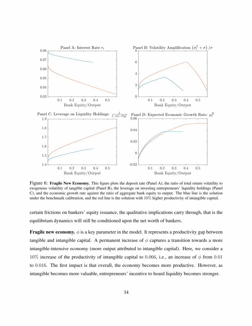
Figure 6: Fragile New Economy. This figure plots the deposit rate (Panel A), the ratio of total return volatility toexogenous volatility of tangible capital (Panel B), the leverage on investing entrepreneurs’ liquidity holdings (PanelC), and the economic growth rate against the ratio of aggregate bank equity to output. The blue line is the solutionunder the benchmark calibration, and the red line is the solution with 10% higher productivity of intangible capital.
certain frictions on bankers’ equity issuance, the qualitative implications carry through, that is the
equilibrium dynamics will still be conditioned upon the net worth of bankers.
Fragile new economy. φ is a key parameter in the model. It represents a productivity gap between
tangible and intangible capital. A permanent increase of φ captures a transition towards a more
intangible-intensive economy (more output attributed to intangible capital). Here, we consider a
10% increase of the productivity of intangible capital to 0.066, i.e., an increase of φ from 0.01
to 0.016. The first impact is that overall, the economy becomes more productive. However, as
intangible becomes more valuable, entrepreneurs’ incentive to hoard liquidity becomes stronger.
34
Panel A of Figure 6 plots the deposit rate. The pattern still holds – as the banking sector ex-
pands, the liquidity premium increases and the interest rate declines. However, the level of interest
rate becomes lower. This is because entrepreneurs assign a higher value to the more productive
intangible capital, and hoard more liquidity for investments. Moreover, the banking sector expands
to a higher level of bank equity-to-output ratio than the benchmark case. When more liquidity is
needed, the economy will have a larger banking sector that issues deposits to meet such demand.
Thus, the model predicts that a transition towards intangible-intensive economy is companied by
the expansion of banking sector. In the past few decades, bank expansion has been documented in
most advanced economies (e.g., Schularick and Taylor (2012)).
A more intangible-intensive economy has a stronger risk amplification mechanism, as shown
in Panel B of Figure 6. The ratio of total return volatility to exogenous volatility of tangible capital
climbed above 6 as the economy goes through a boom and bank expansion. With a stronger
liquidity demand from entrepreneurs, the economy now has an even more functioning feedback
mechanism that works through interest rate and asset price. In particular, Panel A shows that
interest rate is more sensitive to bank equity, i.e., a steeper slope, when φ is higher.
Asset price also becomes more responsive to bank expansion, as shown by the leverage on
entrepreneurs’ liquidity holdings in Panel C, which is a monotonic transformation of qTt . Not
only the slope of qTt , but also its level becomes higher in a more intangible-intensive economy.
This is due to a large liquidity premium and lower discount rate in the tangible capital market.
When intangible capital becomes more productive, the price of tangible capital increases thanks to
stronger liquidity demand of entrepreneurs intermediated by banks. A higher leverage on liquidity
holdings induces entrepreneurs to hold even more liquidity.
The new economy is more fragile. Endogenous risk is generated by a stronger feedback
mechanism that works around the intermediated liquidity premium. The new economy also grows
faster, as shown in Panel D of Figure 6. The intermediated liquidity premium leads to a higher price
of tangible capital, so entrepreneurs are able to increase the leverage on their liquidity holdings
and invest more. Therefore, the model characterizes a risk-return trade-off associated with the
transition to a more intangible-intensive economy – faster growth and more endogenous risk.
35

4 Conclusion
This paper aims to provide a coherent account of several trends in the two decades leading up to the
Great Recession, such as the rising corporate cash holdings, the expansion of financial sector, the
declining interest rate, and the rising prices of risky assets. At the center is the dynamic interaction
between inside money suppliers (banks) and demanders (entrepreneurs).
The money demand of firms arises from investment and capital illiquidity, which are in turn
motivated by the increasing reliance on intangible capital in advanced economies. The financial
stability implications of this structural change has not yet been explored in the existing literature.
This paper proposes a channel of intermediated liquidity premium that links rising asset price and
declining interest rate with the accumulation of endogenous risk in booms. It sheds light on the
recent empirical findings that a long period of banking expansion precedes severe crises. This
new channel of instability and a typical balance-sheet channel reinforce each other, creating a
quantitatively significant amplification mechanism for macro shocks.
The model leaves out the provision of outside money (liquid government securities or central
bank liabilities) for future research. By expanding money supply in booms, the government can
crowd out bank leverage (Krishnamurthy and Vissing-Jorgensen (2015)), and thereby, weaken
the upward spiral in asset price that leads to endogenous risk accumulation. In contrast to the
current practice of monetary expansion in recessions, the optimal supply of outside money can be
procyclical in this setting. However, since entrepreneurs’ incentive to invest is tied to asset price, a
government faces the trade-off between growth and stability.
The model also leaves out banks’ default. The empirical literature on financial crises com-
monly use banks’ default or a high possibility of default as a crisis indicator. A theoretical model
of crisis should ideally accommodate default, and by doing so, it opens up the question of optimal
government intervention, for instance, through equity injection into the banking sector, in order
to prevent a sudden evaporation of inside money. To finance the intervention in bad times, the
government may increase the issuance of outside money (e.g., short-term government securities),
suggesting countercyclical supply of outside money.
36
Appendix I - Proofs of Propositions
Proof of Proposition 1. Entrepreneurs (“firms”) maximize life-time utility, E[∫ +∞
t=0e−ρtdcEt
],
subject to the following wealth (equity) dynamics:
dwEt = −dcEt + µwt wEt dt+ σwt w
Et dZt +
(wEt − wEt
)dNt,
µwt wEt and σwt w
Et are the drift and diffusion terms that depend on choices of tangible capital and
deposit holdings and will be elaborated later. dNt is the increment of the idiosyncratic counting
(Poisson) process. dNt = 1 if a liquidity shock arrives. At the Poisson time, an entrepreneur’s
wealth jumps to
wEt = wEt +
(qIθκ+ qTt (1− θ)κ− 1
1− κ (1− θ) qTt
)mEt .
Note thatwEt is the liquid wealth of entrepreneurs. When analyzing entrepreneurs’ decisions,
we can simply regard cash flows from intangible capital as streams of consumption. We conjecture
that the value function is linear in equity wEt : vEt = ζEt wEt + vI , where ζEt is the marginal value
of liquid wealth, and vI is the present value of consumption flows from intangible capital. In
equilibrium, ζEt follows a diffusion process:
dζEt = ζEt µζtdt+ ζEt σ
ζtdZt,
where ζEt µζt and ζEt σ
ζt are the drift and diffusion terms respectively. Entrepreneurs’ marginal value
of wealth, ζEt , is a summary statistic of their investment opportunity set, which depends on the
overall industry dynamics, so it does not jump when an individual is hit by liquidity shocks.
Under this conjecture, the Hamilton-Jacobi-Bellman (HJB) equation is
ρvEt dt = maxdcEt ∈R,kEt ≥0,mEt ≥0
dcEt − ζEt dcEt + {wEt ζEt µζt + wEt ζEt µ
wt + wtζ
Et σ
ζtσ
wt + λζEt [wt − wt]}dt.
Entrepreneurs can choose any dcEt ∈ R, so ζEt must be equal to one, and thus, I have also confirmed
the value function conjecture.
37
Since ζEt is a constant equal to one, µζt and σζt are both zero. The HJB equation is simplified:
ρvEt dt = maxkEt ≥0,mEt ≥0
µwt wEt dt+ λdt
(qIθκ+ qTt (1− θ)κ− 1
1− κ (1− θ) qTt
)mEt . (18)
Wealth drift has production, value change of tangible capital holdings, and deposit return:
µwt wEt dt = αkEt dt+ Et
(qTt+dtk
Et+dt − qTt kEt
)︸ ︷︷ ︸
Et[drTt ]qTt kEt
+ rtmEt dt.
Let dψEt denote the Lagrange multiplier of the budget constraint, qTt kTt +m
Et ≤ wEt . The first-order
condition (F.O.C.) for optimal deposit holdings per unit of capital is: mEt ≥ 0, and
mEt
{rtdt+ λdt
(qIθκ+ qTt (1− θ)κ− 1
1− κ (1− θ) qTt
)− dψEt
}= 0.
The F.O.C. for optimal tangible capital holdings is : kEt ≥ 0, and
−Et[drTt]+ dψEt = 0.
Substituting these optimality conditions into the HJB equation, we have
ρvEt dt = wEt dψEt .
Because ζEt = 1, vEt = wEt , and dψEt = ρdt. Substituting dψEt = ρdt into the F.O.C. for mEt , we
have
ρ− rt = λ
(qIθκ+ qTt (1− θ)κ− 1
1− κ (1− θ) qTt
).
Substituting dψt = ρdt into the F.O.C. for kEt and rearranging the equation, we have
Et[drTt]= ρdt.
38

Proof of Proposition 2. Conjecture that the bank’s value function takes the linear form: vBt =
qBt nBt . In equilibrium, the marginal value of equity, qBt , evolves as follows
dqBt = qBt µBt dt+ qBt σ
Bt dZt.
Define dyBt = dcBt /nBt , the consumption-to-wealth ratio of bankers. Under the conjectured func-
tional form, the HJB equation is
ρvBt dt = maxdyBt ∈R
{(1− qBt
)I{dyBt >0}n
Bt dy
Bt
}+ µBt q
Bt n
Bt +
maxxBt ≥0
{rt + xBt
(Et[drTt]− rt
)+ xBt σ
Bt
(σTt + σ
)}qBt n
Bt ,
where γBt = −σBt . Dividing both sides by qBt nBt , we eliminate nBt in the HJB equation,
ρ = maxdyBt ∈R
{(1− qBt
)
qBtI{dyBt >0}dy
Bt
}+ µBt +
maxxBt ≥0
{rt + xBt
(Et[drTt]− rt
)+ xBt σ
Bt
(σTt + σ
)},
and thus, confirm the conjecture of linear value function. The indifference condition for xBt gives
the equation in Proposition 2.
Proof of Proposition 3. Following Brunnermeier and Sannikov (2014), I derive the stationary
probability density. Probability density of ηt at time t, p (η, t), has Kolmogorov forward equation
∂
∂tp (η, t) = − ∂
∂η(ηµη (η) p (η, t)) +
1
2
∂2
∂η2(η2ση (η)2 p (η, t)
).
Note that in a Markov equilibrium, µηt and σηt are functions of ηt. A stationary density is a solution
to the forward equation that does not vary with time (i.e. ∂∂tp (η, t) = 0). So I suppress the time
variable, and denote stationary density as p (η). Integrating the forward equation over η, p (η)
solves the following first-order ordinary differential equation within the two reflecting boundaries:
0 = C − ηµη (η) p (η) + 1
2
d
dη
(η2ση (η)2 p (η)
), η ∈
[η, η]
.
39
The integration constantC is zero because of the reflecting boundaries. The boundary condition for
the equation is the requirement that probability density is integrated to one (i.e.∫ ηηp (η) dη = 1).
Next, I solve the expected time to reach from η. Define fη0 (η) the expected time it takes to
reach η0 starting from η ≤ η0. Define g (η0) = fη0(η)
the expected time to reach η0 from η. One
has to reach η ∈(η, η0
)first and then reach η0 from η. Therefore, g (η) + fη0 (η) = g (η0). Since
g (η0) is constant, we differentiate both sides to have g′ (η) = −f ′η0 (η) and g′′ (η) = −f ′′η0 (η).From ηt, the expected time to reach η0, denoted by fη0 (ηt), is decomposed into s − t, and
Et[fη0 (ηs)
], i.e., the expected time to reach η0 from ηs (s ≥ t) after s − t has passed. We have
fη0 (ηt) equal to Et[fη0 (ηs)
]+ s − t. Therefore, t + fη0 (ηt) is a martingale, so fη0 satisfies the
ordinary differential equation: 1 + f ′η0 (η)µη (η) + ση(η)2
2f ′′η0 (η) = 0. Therefore, g (η) must satisfy
1− g′ (η)µη (η)− ση (η)2
2g′′ (η) = 0.
It takes no time to reach η, so g(η)= 0. Moreover, since η is a reflecting boundary, g′
(η)= 0.
Proof of Proposition 4. The system of ordinary differential equations is constructed in detail in
Appendix II. The boundary conditions are explained in the main text.
Appendix II - Solving the Equilibrium
The fully solved Markov equilibrium is a set of functions that map ηt to the values of endogenous
variables, such as tangible capital price, interest rate, bank leverage, and entrepreneurs’ deposit
holdings. In the description of solution method, time subscripts are suppressed to save notations.
First, we construct a mapping from η, qB (η), qT (η), dqB (η) /dη, and dqT (η) /dη to the
second-order derivatives, d2qB (η) /dη2 and d2qT (η) /dη, i.e., a system of second-order ordinary
differential equations.
Given qT , Proposition 1 solves the liquidity premium, ρ − r and deposit rate r. For small
values of η, consider the case where banks do not hold all tangible capital, so ρ = r−σB(σT + σ
).
40

By Ito’s lemma,
σT = εTση andσB = εBση.
where εT = dqT /qT
dη/ηand εB = dqB/qT
dη/η. Since ρ − r is a function of qT , we substitute the decompo-
sition of σT and σB into ρ = r − σB(σT + σ
)to obtain a quadratic equation of ση, and the roots
are
ση =−εBσ ±
√(εBσ)2 − 4εBεT (ρ− r)
2εBεT.
Because εB < 0, εT > 0, and ρ ≥ r, the only positive root is
ση =−εBσ −
√(εBσ)2 − 4εBεT (ρ− r)
2εBεT.
Because ση = xB(σT + σ
)− σ, we can solve
xB =ση + σ
σηεT + σ. (19)
Next, we need to check whether xBNB ≤ qTKT , or equivalently, xBη ≤ qT (1− θ). If this
condition does not hold, we are at point where banks are large enough to hold all tangible capital,
so we set xB = qT (1− θ) /η, and solve ση using Equation (19). Once xB and ση are solved, σB
and σT can be solved by Ito’s lemma, and bankers’ required risk compensation, −σB(σT + σ
).
Next, we solve the drift terms of bankers’ wealth,
µN = xBE[drT]+(1− xB
)r,
and the diffusion term
σN = xB(σT + σ
).
From Equation (11), we can solve µK . And from Equation (12),
µη = µN − µK − σNσ + σ2.
41
To solve the second-order derivatives, d2qB (η) /dη2 and d2qT (η) /dη, we use bankers’ HJB equa-
tion (after substituting the first-order conditions),
µB = ρ− r,
and bankers’ optimality condition for tangible capital holdings in Proposition 2,
µT = r − σB(σT + σ
)− σTσ + δ − α
qT,
so from Ito’s lemma,
d2qT
dη2= 2qT
(µT − εTµη
)
(σηη)2, and,
d2qB
dη2= 2qB
(µB − εBµη
)
(σηη)2.
The procedure constructs a mapping from η, qB (η), qT (η), dqB (η) /dη, and dqT (η) /dη
to the second-order derivatives, d2qB (η) /dη2 and d2qT (η) /dη. The five boundary conditions
in Proposition 4 pin down a unique solution to the two second-order ODEs and one endogenous
boundary (bankers’ consumption boundary η).
42
ReferencesAdrian, T. and H. S. Shin (2010a). The changing nature of financial intermediation and the financial
crisis of 2007-09. Staff Reports 430, Federal Reserve Bank of New York.
Adrian, T. and H. S. Shin (2010b). Liquidity and leverage. Journal of Financial Intermedia-tion 19(3), 418 – 437. Risk Transfer Mechanisms and Financial Stability.
Almeida, H. and M. Campello (2007). Financial constraints, asset tangibility, and corporate in-vestment. Review of Financial Studies 20(5), 1429–1460.
Andrade, G. and S. N. Kaplan (1998). How costly is financial (not economic) distress? evidencefrom highly leveraged transactions that became distressed. The Journal of Finance 53(5), 1443–1493.
Atkeson, A. and P. J. Kehoe (2005). Modeling and measuring organization capital. Journal ofPolitical Economy 113(5), 1026–1053.
Azar, J., J.-F. Kagy, and M. C. Schmalz (2016). Can changes in the cost of carry explain thedynamics of corporate cash holdings? Review of Financial Studies, forthcoming.
Baron, M. and W. Xiong (2016). Credit expansion and neglected crash risk. Quarterly Journal ofEconomics, forthcoming.
Basak, S. and D. Cuoco (1998). An equilibrium model with restricted stock market participation.Review of Financial Studies 11(2), 309–341.
Bates, T. W., K. M. Kahle, and R. M. Stulz (2009). Why do U.S. firms hold so much more cashthan they used to? The Journal of Finance 64(5), 1985–2021.
Begenau, J. and B. Palazzo (2015). Firm selection and corporate cash holdings. 2015 MeetingPapers 1047, Society for Economic Dynamics.
Bernanke, B. S. (1983). Nonmonetary effects of the financial crisis in the propagation of the greatdepression. The American Economic Review 73(3), 257–276.
Bernanke, B. S. and A. S. Blinder (1992). The federal funds rate and the channels of monetarytransmission. The American Economic Review 82(4), 901–921.
Bernanke, B. S. and M. Gertler (1989). Agency costs, net worth, and business fluctuations. TheAmerican Economic Review 79(1), 14–31.
Bolton, P., H. Chen, and N. Wang (2011). A unified theory of Tobin’s q, corporate investment,financing, and risk management. The Journal of Finance 66(5), 1545–1578.
43
Bolton, P. and X. Freixas (2000). Equity, bonds, and bank debt: Capital structure and financialmarket equilibrium under asymmetric information. Journal of Political Economy 108(2), 324–351.
Bolton, P., T. Santos, and J. A. Scheinkman (2018). Savings gluts and financial fragility. Workingpaper, Columbia University.
Bordo, M., B. Eichengreen, D. Klingebiel, M. S. Martinez-Peria, and A. K. Rose (2001). Is thecrisis problem growing more severe? Economic Policy: A European Forum 16(32), 53–82.
Brunnermeier, M. K. and Y. Sannikov (2014, February). A macroeconomic model with a financialsector. American Economic Review 104(2), 379–421.
Brunnermeier, M. K. and Y. Sannikov (2016). The I theory of money. Working paper, PrincetonUniversity.
Caballero, R. J., E. Farhi, and P.-O. Gourinchas (2008). An equilibrium model of ”global imbal-ances” and low interest rates. American Economic Review 98(1), 358–93.
Caballero, R. J. and A. Krishnamurthy (2009, May). Global imbalances and financial fragility.American Economic Review 99(2), 584–88.
Carlson, M., B. Duygan-Bump, F. Natalucci, B. Nelson, M. Ochoa, J. Stein, and S. Van den Heuvel(2016). The demand for short-term, safe assets and financial stability: Some evidence andimplications for central bank policies. International Journal of Central Banking, forthcoming.
Cavalcanti, R. d. O. and N. Wallace (1999). A model of private bank-note issue. Review ofEconomic Dynamics 2(1), 104 – 136.
Corrado, C., C. Hulten, and D. Sichel (2005). Measuring capital and technology: An expandedframework. In C. Corrado, J. Haltiwanger, and D. Sichel (Eds.), Measuring Capital in the NewEconomy, pp. 11–46. San Diego: University of Chicago Press.
Corrado, C. A. and C. R. Hulten (2010, May). How do you measure a ”technological revolution”?American Economic Review 100(2), 99–104.
Dang, T. V., G. Gorton, B. Holmstrom, and G. Ordonez (2014, June). Banks as secret keepers.Working Paper 20255, National Bureau of Economic Research.
DeMarzo, P. M. and D. Duffie (1999). A liquidity-based model of security design. Economet-rica 67(1), 65–99.
Denis, D. J. and V. Sibilkov (2010). Financial constraints, investment, and the value of cashholdings. Review of Financial Studies 23(1), 247–269.
44
Di Tella, S. (2014). Uncertainty shocks and balance sheet recessions. Working paper, StanfordUniversity Graduate School of Business.
Diamond, D. W. (1984). Financial intermediation and delegated monitoring. The Review of Eco-nomic Studies 51(3), 393–414.
Duchin, R. (2010). Cash holdings and corporate diversification. The Journal of Finance 65(3),955–992.
Duchin, R., T. Gilbert, J. Harford, and C. M. Hrdlicka (2017). Precautionary savings with riskyassets: When cash is not cash. The Journal of Finance 72(2), 793–852.
Eisfeldt, A. and A. Rampini (2009). Financing shortfalls and the value of aggregate liquidity.Working paper, Duke University.
Eisfeldt, A. L. (2007). Smoothing with liquid and illiquid assets. Journal of Monetary Eco-nomics 54(6), 1572 – 1586.
Eisfeldt, A. L. and D. Papanikolaou (2014). The value and ownership of intangible capital. Amer-ican Economic Review 104(5), 189–94.
Falato, A. and J. W. Sim (2014). Why Do Innovative Firms Hold So Much Cash? Evidence fromChanges in State R&D Tax Credits. Finance and Economics Discussion Series 2014-72, Boardof Governors of the Federal Reserve System (U.S.).
Farhi, E. and J. Tirole (2012). Bubbly liquidity. The Review of Economic Studies.
Friedman, M. and A. J. Schwartz (1963). A Monetary History of the United States, 1867-1960.Princeton, N.J.: Princeton University Press.
Froot, K. A., D. S. Scharfstein, and J. C. Stein (1993). Risk management: Coordinating corporateinvestment and financing policies. The Journal of Finance 48(5), 1629–1658.
Gorton, G. (2010). Slapped by the Invisible Hand: The Panic of 2007. New York, N.Y.: Oxfor-dUniversity Press.
Gorton, G., S. Lewellen, and A. Metrick (2012, May). The safe-asset share. American EconomicReview 102(3), 101–06.
Gorton, G. and A. Metrick (2012). Securitized banking and the run on repo. Journal of FinancialEconomics 104(3), 425 – 451. Market Institutions, Financial Market Risks and Financial Crisis.
Gorton, G. and G. Ordonez (2014, February). Collateral crises. American Economic Re-view 104(2), 343–78.
45
Gorton, G. and G. Pennacchi (1990). Financial intermediaries and liquidity creation. The Journalof Finance 45(1), 49–71.
Graham, J. R. and M. T. Leary (2015). The evolution of corporate cash. Working paper, DukeUniversity.
Greenwood, R. and D. Scharfstein (2013, May). The growth of finance. Journal of EconomicPerspectives 27(2), 3–28.
Gurley, J. G. and E. S. Shaw (1960). Money in a Theory of Finance. Washington, D.C.: BrookingsInstitution.
Hall, B. H. (1992). Investment and research and development at the firm level: Does the source offinancing matter? Working Paper 4096, National Bureau of Economic Research.
Hall, B. H. and J. Lerner (2009). The financing of R&D and innovation. Working Paper 15325,National Bureau of Economic Research.
Hart, O. and J. Moore (1994). A theory of debt based on the inalienability of human capital. TheQuarterly Journal of Economics 109(4), 841–879.
Hart, O. and L. Zingales (2014). Banks are where the liquidity is. Working paper, Harvard Uni-versity.
He, Z. and P. Kondor (2016). Inefficient investment waves. Econometrica 84(2), 735–780.
He, Z. and A. Krishnamurthy (2013). Intermediary asset pricing. American Economic Re-view 103(2), 732–70.
Himmelberg, C. P. and B. C. Petersen (1994). R&D and internal finance: A panel study of smallfirms in high-tech industries. The Review of Economics and Statistics 76(1), 38–51.
Holmstrom, B. (2012). The nature of liquidity provision: When ignorance is bliss. In PresidentialAddress, Econometric Society, ASSA meetings, Chicago.
Holmstrom, B. and J. Tirole (1997). Financial intermediation, loanable funds, and the real sector.The Quarterly Journal of Economics 112(3), 663–691.
Holmstrom, B. and J. Tirole (1998). Private and public supply of liquidity. Journal of PoliticalEconomy 106(1), 1–40.
Holmstrom, B. and J. Tirole (2001). LAPM: A liquidity-based asset pricing model. The Journalof Finance 56(5), 1837–1867.
46
Jorda, O., M. Schularick, and A. M. Taylor (2013). When credit bites back. Journal of Money,Credit and Banking 45(s2), 3–28.
Kiyotaki, N. and J. Moore (1997). Credit cycles. Journal of Political Economy 105(2), 211–248.
Kiyotaki, N. and J. Moore (2000). Inside money and liquidity. Working paper, London School ofEconomics.
Kiyotaki, N. and J. Moore (2005). Lawrence R. Klein Lecture: Liquidity and asset prices. Inter-national Economic Review 46(2), 317–349.
Kiyotaki, N. and J. Moore (2012). Liquidity, business cycles, and monetary policy. Working paper,Princeton University.
Kiyotaki, N. and R. Wright (1989). On money as a medium of exchange. Journal of PoliticalEconomy 97(4), 927–954.
Klimenko, N., S. Pfeil, J.-C. Rochet, and G. D. Nicolo (2016). Aggregate bank capital and creditdynamics. Swiss Finance Institute Research Paper Series 16-42.
Kocherlakota, N. R. (1998). Money is memory. Journal of Economic Theory 81(2), 232 – 251.
Krishnamurthy, A. and T. Muir (2016). How credit cycles across a financial crisis. Working paper,Stanford University Graduate School of Business.
Krishnamurthy, A. and A. Vissing-Jorgensen (2015). The impact of treasury supply on financialsector lending and stability. Journal of Financial Economics 118(3), 571 – 600.
Krusell, P. and A. A. Smith (1998). Income and wealth heterogeneity in the macroeconomy.Journal of Political Economy 106(5), 867–896.
Lagos, R. (2008). inside and outside money. In S. N. Durlauf and L. E. Blume (Eds.), The NewPalgrave Dictionary of Economics. Basingstoke: Palgrave Macmillan.
Levine, R. (1997). Financial development and economic growth: Views and agenda. Journal ofEconomic Literature 35(2), 688–726.
Li, S., T. M. Whited, and Y. Wu (2016). Collateral, taxes, and leverage. Review of FinancialStudies 29(6), 1453–1500.
Longstaff, F. A. and J. Wang (2012). Asset pricing and the credit market. Review of FinancialStudies 25(11), 3169–3215.
Lopez-Salido, D., J. C. Stein, and E. Zakrajsek (2015). Credit-market sentiment and the businesscycle. Working paper, Harvard University.
47

Lucas, R. E. J. and J. P. Nicolini (2015). On the stability of money demand. Journal of MonetaryEconomics 73, 48 – 65.
Mankiw, N. and S. P. Zeldes (1991). The consumption of stockholders and nonstockholders.Journal of Financial Economics 29(1), 97 – 112.
McGrattan, E. R. (2016). Intangible capital and measured productivity. Working paper, Universityof Minnesota.
McGrattan, E. R. and E. C. Prescott (2010, September). Technology capital and the us currentaccount. American Economic Review 100(4), 1493–1522.
Moll, B. (2014, October). Productivity losses from financial frictions: Can self-financing undocapital misallocation? American Economic Review 104(10), 3186–3221.
Moreira, A. and A. Savov (2017). The macroeconomics of shadow banking. The Journal ofFinance 72(6), 2381–2432.
Opler, T., L. Pinkowitz, R. Stulz, and R. Williamson (1999). The determinants and implications ofcorporate cash holdings. Journal of Financial Economics 52(1), 3 – 46.
Ostroy, J. M. and R. M. Starr (1990). Chapter 1 the transactions role of money. Volume 1 ofHandbook of Monetary Economics, pp. 3 – 62. Elsevier.
Perez-Orive, A. and A. Caggese (2017). Capital Misallocation and Secular Stagnation. 2017Meeting Papers 382, Society for Economic Dynamics.
Peters, R. H. and L. A. Taylor (2016). Intangible capital and the investment-q relation. Journal ofFinancial Economics, forthcoming.
Piazzesi, M. and M. Schneider (2016). Payments, credit and asset prices. Working paper, StanfordUniversity.
Pinkowitz, L., R. M. Stulz, and R. Williamson (2015). Do u.s. firms hold more cash than foreignfirms do? Review of Financial Studies.
Pozsar, Z. (2011). Institutional cash pools and the Triffin dilemma of the u.s. banking system.Working paper WP/11/190, International Monetary Fund.
Pozsar, Z. (2014). Shadow banking: The money view. Working paper 14-04, Office of FinancialResearch.
Protter, P. E. (1990). Stochastic Integration and Differential Equations. New York: Springer-Verlag.
48
Quadrini, V. (2017). Bank liabilities channel. Journal of Monetary Economics 89, 25 – 44.Carnegie-Rochester-NYU Conference Series on the Macroeconomics of Liquidity in CapitalMarkets and the Corporate Sector.
Rajan, R. G. and L. Zingales (1998). Financial dependence and growth. The American EconomicReview 88(3), 559–586.
Rampini, A. A. and S. Viswanathan (2015). Financial intermediary capital. Working paper, DukeUniversity.
Reinhart, C. M. and K. S. Rogoff (2009). This Time Is Different: Eight Centuries of FinancialFolly. Princeton, NJ: Princeton University Press.
Schularick, M. and A. M. Taylor (2012, April). Credit booms gone bust: Monetary policy, leveragecycles, and financial crises, 1870-2008. American Economic Review 102(2), 1029–61.
Shleifer, A. and R. W. Vishny (2010, December). Fire sales in finance and macroeconomics.Working Paper 16642, National Bureau of Economic Research.
Stein, J. C. (2012). Monetary policy as financial stability regulation. The Quarterly Journal ofEconomics 127(1), 57–95.
Van den Heuvel, S. J. (2002). The bank capital channel of monetary policy. Working paper, TheWharton School of the University of Pennsylvania.
Williamson, S. and R. Wright (2010). Chapter 2 - New monetarist economics: Models. Volume 3of Handbook of Monetary Economics, pp. 25 – 96. Elsevier.
Woodford, M. (1990). Public debt as private liquidity. The American Economic Review 80(2),382–388.
49