mathematics

Article

Fractional Vertical Infiltration

Carlos Fuentes 1 , Fernando Alcántara-López 2,* , Antonio Quevedo 1 and Carlos Chávez 3

�����������������

Citation: Fuentes, C.; Alcántara-López,

F.; Quevedo, A.; Chávez, C. Fractional

Vertical Infiltration. Mathematics 2021,

9, 383. https://doi.org/10.3390/

math9040383

Academic Editor: Duarte Valério

Received: 28 January 2021

Accepted: 10 February 2021

Published: 14 February 2021

Publisher’s Note: MDPI stays neutral

with regard to jurisdictional claims in

published maps and institutional affil-

iations.

Copyright: © 2021 by the authors.

Licensee MDPI, Basel, Switzerland.

This article is an open access article

distributed under the terms and

conditions of the Creative Commons

Attribution (CC BY) license (https://

creativecommons.org/licenses/by/

4.0/).

1 Mexican Institute of Water Technology, Paseo Cuauhnáhuac Núm. 8532, Jiutepec, Morelos 62550, Mexico;cbfuentesr@gmail.com (C.F.); jose_quevedo@tlaloc.imta.mx (A.Q.)

2 Department of Mathematics, Faculty of Science, National Autonomous University of México,Av. Universidad 3000, Circuito Exterior S/N, Delegación Coyoacán 04510, Ciudad de México, Mexico

3 Water Research Center, Department of Irrigation and Drainage Engineering, Autonomous University ofQuerétaro, Cerro de las Campanas SN, Col. Las Campanas 76010, Querétaro, Mexico; chagcarlos@uaq.mx

* Correspondence: alcantaralopez@comunidad.unam.mx

Abstract: The infiltration phenomena has been studied by several authors for decades, and numericaland approximate results have been shown through the asymptotic solution in short and long times.In particular, it is worth highlighting the works of Philip and Parlange, who used time and volumetriccontent as independent variables and space as a dependent variable, and found the solution as apower series in t1/2 that is valid for short times. However, several studies show that these modelsare not applicable to anomalous flows, in which case the application of fractional calculus is needed.In this work, a fractional time derivative of a Caputo type is applied to model anomalous infiltrationphenomena. Fractional horizontal infiltration phenomena are studied, and the fractional Boltzmanntransform is defined. To study fractional vertical infiltration phenomena, the asymptotic behavior isdescribed for short and long times considering an arbitrary diffusivity and hydraulic conductivity.Finally, considering a constant flux-dependent relation and a relation between diffusivity and hy-draulic conductivity, a fractional cumulative infiltration model applicable to various types of soil isbuilt; its solution is expressed as a power series in tν/2, where ν ∈ (0, 2) is the order of the fractionalderivative. The results show the effect of superdiffusive and subdiffusive flows in different typesof soil.

Keywords: asymptotic solution; parlange equations; Darcy’s law; fractional Caputo derivative

1. Introduction

More than a century ago, Green and Ampt [1] laid the bases for describing the infiltra-tion process; to this day, there are still open problems in the area, where existing modelsin the literature cannot explain laboratory results [2]. As one of the pioneers in the area,Philip [3] describes the infiltration phenomenon as a Fokker–Planck type equation. In asemi-infinite domain, homogeneous, its form is

∂θ

∂t= ∇ · (D(θ)∇θ)− dK

dθ· ∂θ

∂z, (1)

where θ is the volumetric water content, D(θ) is the hydraulic diffusivity, K(θ) is thehydraulic conductivity, θ0 is the initial volumetric water content, θs is the volumetric watercontent at saturation, t is the time, and z is the spatial variable taken positive downward.

In particular, when considering horizontal infiltration:

∂θ

∂t=

∂

∂x

(D(θ)

∂θ

∂x

), (2)

with initial conditions

t = 0, x > 0, θ = θ0,t ≥ 0, x = 0, θ = θs,

(3)

Mathematics 2021, 9, 383. https://doi.org/10.3390/math9040383 https://www.mdpi.com/journal/mathematics

Mathematics 2021, 9, 383 2 of 14

Equations (2) and (3) reduces to

−φ

2=

ddθ

(D(θ)

dφ/dθ

), (4)

φ = 0, θ = θs,φ→ ∞, θ = θ0,

(5)

by introducing the Boltzmann transform [4].On the other hand, when considering vertical infiltration,

∂θ

∂t=

∂

∂z

(D(θ)

∂θ

∂z

)− dK

dθ

∂θ

∂z, (6)

t = 0, z > 0, θ = θ0,t ≥ 0, z = 0, θ = θs,

(7)

Philip [5] applied the implicit function theorem and rewrote Equation (6) as

∂z∂t

=∂q∂θ

, q(θ, t) = − D(θ)

∂z/∂θ+ K(θ), (8)

where q = q(θ, t) is the Darcy flow; Philip proved that, for short times, the solution ofEquation (8) is sought in the form

z(θ, t) = φ(θ)t1/2 + χ(θ)t + Ψ(θ)t3/2 + ω(θ)t2 + · · · (9)

where each term function of θ in the series is defined from integro-differential equationswhose expression considering fractional calculus will be shown in Section 4. In particular,the first term in the series (9), φ(θ), matches the solution of the horizontal infiltrationproblem, Equation (4).

However, Philip did not work with the radius of convergence of the series, a problemthat remains open to date, but suggests that the range of useful convergence is tgrav, whereit is obtained from dimensional analysis that gravity effects are as great as capillarityeffects, namely,

t < tgrav :=(

SKs − K0

)2, (10)

where Ks = K(θs) is the hydraulic conductivity at saturation, K0 = K(θ0) is the initialhydraulic conductivity, and S is the sorptivity defined by

S =∫ θs

θ0

φ(θ)dθ, (11)

where φ(θ) is the Boltzmann transform defined by the differential Equation (4).Likewise, Philip [5] proves that, for long times, the solution of Equation (8) has

the form

z(θ, t) = ζ(θ) +Ks − K0

θs − θ0t, (12)

where ζ(θ) is a function of volumetric water content and can be expressed in terms ofdiffusivity and hydraulic conductivity as

ζ(θ) =∫ θa

θ

(θs − θ0)D(θ̄)dθ̄

(Ks − K0)(θ̄ − θ0)− (K(θ̄)− K0)(θs − θ0), (13)

where θa = θs−∆θ and ∆θ is a definite small positive quality; the calculus of ζ, Equation (13),should be done carefully since, in general, ζ has singularities at θ = θs, θ0.

Mathematics 2021, 9, 383 3 of 14

Philip showed that, when water is applied to uniform soils, it is sufficient to retainonly two terms of the series to obtain an adequate description of the vertical infiltration.Talsma and Parlange [6] proved that sorptivity S and conductivity at saturation Ks werethe soil parameters necessary for the two terms of the Philip series; in addition, the one-dimensional infiltration equation is more sensitive to soil heterogeneity than its equivalentsin two or three dimensions.

Later, Parlange et al. [7] showed that adding a third parameter to the series is sufficientto describe cumulative infiltration accurately, where this extra parameter is representativeof the type of soil in which water infiltration takes place.

Haverkamp et al. [8] recognize that the infiltration process can be described eitherby solving the Richards equation or by considering cumulative infiltration. They chosethe second option. Since previous models used highly time-dependent parameters [9],they developed an equation for infiltration subject to head boundary conditions consider-ing time-independent parameters, which takes into account the possibility of an infinitediffusivity near saturation.

Fuentes et al. [10] analyzed the constraints on different fitting parameters used in awater retention equation and hydraulic conductivity using the infiltration equations todescribe several soils types. Later, Fuentes et al. [11] calculated the analytical solution forvertical infiltration considering a constant diffusivity and a hydraulic conductivity resultingfrom a linear combination of linear and quadratic functions of volumetric water content.They showed that their model can also be applied to soils that do not necessarily meetthe hypotheses for his deduction. On the other hand, using a numerical approximation,Saucedo et al. [12] verified the contact time hypothesis to describe water transfer in melgasirrigation by coupling the Saint– Venant and Richards equations.

Over the years, the Philip power series has been applied in different contexts, such asfalling head ponded infiltration [13], variable head ponded infiltration on flat surfaces [14],and variable head ponded infiltration on sloping surfaces [15], to name a few. In particular,in the last work, they showed that sorptivity is independent of the slope angle and thatcumulative infiltration normal to the slope decreases with increasing slope angles.

Recently, cumulative infiltration was used to describe the effect of pressure head andsoil bulk density on moistube irrigation [16]. It was concluded that infiltration index α isnegatively correlated with pressure head but positively with soil bulk density, while theinfiltration coefficient K was positively correlated with the pressure head but negativelywith the soil bulk density.

Likewise, water infiltration has been used to calculate infiltrated depth evolutionand humidity profiles by coupling the Saint–Venant and Richards equations with furrowboundary conditions [17]. Considering this model, the relationship between the optimalirrigation flow and the length of the border for different types of soil was found [18].

These examples show the wide range of applications that the Philip power series hasfor water infiltration in different types of soil; in this sense, it goes without saying howuseful infiltration models are in developing an effective design and evaluating surfaceirrigation systems, whether they are physical (such as Philip’s [5] and Richards’ [19] mod-els), semi-empirical (such as Holtan’s [20] model) or empirical models (such as Sihag’s [21]model) [22].

When studying non-heterogeneous soils, the transport phenomenon in soils is rec-ognized as being fundamentally stochastic [23,24]. Moreover, to apply equations, e.g.,Richards or Philip power series, it is necessary to assume that water moves in a Brown-ian motion [25]; however, several studies have shown that this assumption is not validand that anomalous flows can be created. The reason behind these anomalous flows isexplained by several authors; they argue that constraints can be imposed by the structureof the porous media or by solute–surface interactions, resulting in Lévy flights due to thepresence of highly conductive fractures, channels, or macropores or because the infiltrationfront undergoes jerky movements [26–28]. Thus, the application of fractional derivativeswas considered to explain the anomalous behavior.

Mathematics 2021, 9, 383 4 of 14

Pachepsky et al. [29] considered water transport in horizontal soil columns andgeneralized the Richards equation to include a fractional time derivative and solved itby generalizing the Boltzmann transform. Sun et al. [30] considered the same problem;however, noting that the fractional derivative fails with the chain rule, they considereda fractal derivative and showed that their results exhibited an anomalous Boltzmanntransform, attributed to the fractal nature of the heterogeneous media.

Generalizing the Fokker–Planck type equation, Su [31] applied the fractional deriva-tive to present a fractional cumulated infiltration into swelling soils where convectiondominates, applying the most linear hydraulic conductivity. Subsequently [32], he general-ized these results to include mobile and immobile zones with and without gravity effects.Later [33], he introduced mass–time fractional derivatives for swelling-shrinking soils andspace–time fractional derivatives for non-swelling soils, applying for mobile zones with orwithout immobile zones by using power functions for diffusivity and hydraulic conductiv-ity. Physically, the spatial fractional derivative means that the concentration change at thepoint of observation depends on upstream concentrations, while the temporal fractionalderivative implies that the concentration change at the point of observation depends onthe prior concentration loading [34].

In the present work, a model for infiltration is developed using a fractional calculationas a tool to incorporate the anomalous behavior in the flow of water. Anomalous horizontalinfiltration will first be studied to later extend these results to study anomalous verticalinfiltration, where asymptotic solutions will be given for short and long times. Finally,a relationship between conductivity and diffusivity will be assumed to yield a validanomalous infiltration model for all times.

The work is developed in the following way: Section 2 describes the mathematicaltools from fractional calculus that will be implemented; Section 3 develops the equationfor the fractional horizontal infiltration considering x = x(θ, t) as the dependent variableand θ, t as independent variables; Section 4 extends the results of the previous sectionby studying vertical infiltration phenomena for both arbitrary diffusivity and hydraulicconductivity through the asymptotic solution in short times and long times; Section 5considers, as additional hypotheses, a constant flux-dependant relationship and a relationbetween diffusivity and hydraulic conductivity to build a model for fractional cumulativeinfiltration, where its solution is developed for short times expressed as a power series oftν/2, where ν is the order of the time fractional derivative with 0 < ν < 2; finally, Section 6summarizes the conclusions reached in this work.

2. Fractional Calculus

At present, there is a great diversity of fractional derivatives such as Riemann–Liouville, Caputo, Grünwald, Marchaud, and Riez, among many others. In this section,the basis of fractional calculus that will be applied for the development of this work will bedescribed. For more information regarding these properties, see [35–37].

Definition 1. Let −∞ < a < ∞. The Riemann–Liouville fractional integral RL Iαa+ f of order

α ∈ R is defined by (RL Iα

a+ f)(x) =

1Γ(α)

∫ x

a(x− t)α−1 f (t)dt, x > a, (14)

where Γ(α) is the gamma function applied to α defined by

Γ(α) =∫ ∞

0tα−1e−tdt, <e(α) > 0. (15)

The fractional integral is the basis from which various forms of fractional derivativeare defined:

Definition 2. The Riemann–Liouville fractional derivative RLDαa+y of order α ∈ R is defined by

Mathematics 2021, 9, 383 5 of 14

(RLDα

a+y)(x) =

dn

dxn

(RL In−α

a+ y)(x) =

1Γ(n− α)

dn

dxn

∫ x

a(x− t)n−α−1y(t)dt, (16)

where n ∈ N with n− 1 < α ≤ n.

Definition 3. The Caputo fractional derivative CDαa+y of order α ∈ R is defined by

(CDα

a+y)(x) =

(RL In−α

a+dn

dxn y)(x) =

1Γ(n− α)

∫ x

a(x− t)n−α−1y(n)(t)dt, (17)

where n ∈ N with n− 1 < α ≤ n and y(n) is the n-th derivative.

The Riemann–Liouville fractional derivative and the Caputo fractional derivative aretwo of the most widely used definitions in fractional calculus; the first because it can beimplemented numerically with ease due to the Grünwald-Letnikov algorithm, althoughit does not allow for the use of the usual initial conditions, while the second allows theclassical initial conditions to be implemented when solving fractional differential equations.

In addition, both definitions of the fractional derivative are related by

(CDα

a+y)(x) =

(RLDα

a+

[y(t)−

n−1

∑k=0

y(k)(a)k!

(t− a)k

])(x); (18)

it follows from Equation (18) that both definitions of the fractional derivative are equivalentif y(k)(a) = 0 for k = 0, 1, . . . , n− 1.

In particular, if α, β ∈ R, it can be verified directly from definitions 2 and 3 that(RLDα

a+(t− a)β)(x) =

(CDα

a+(t− a)β)(x) =

Γ(β + 1)Γ(β− α + 1)

(x− a)β−α. (19)

Likewise, the Caputo fractional derivative and the Riemann–Liouville fractionalintegral act among themselves, generalizing the fundamental theorem of calculus, where,for sufficiently good conditions of y(t), it is satisfied that

(RL Iα

a+CDα

a+y)(x) = y(x)−

n−1

∑k=0

y(k)(a)k!

(x− a)k. (20)

3. Fractional Horizontal Infiltration

In this section, the fractional horizontal infiltration equation is developed and solvedby replacing the time derivative by the Caputo fractional derivative and neglecting theterm associated with the gravitational field.

Note that applying the implicit function theorem to Equation (2), to express θ and t asindependent variables and x = x(θ, t) as a dependent variable, it follows that

∂x∂t

=∂q∂θ

, q(θ, t) = − D(θ)

∂x/∂θ, (21)

where q = q(θ, t) is the Darcy flow.Therefore, the fractional differential equation that describes the anomalous horizontal

infiltration is

τν−1c

∂νx∂tν

+∂

∂θ

[D(θ)

∂x/∂θ

]= 0, (22)

Mathematics 2021, 9, 383 6 of 14

where ν ∈ (0, 2) is the order of the fractional derivative, and τc is a constant introducedto maintain dimensional balance with units of time and initial and boundary conditionsshown in Equation (3).

It can be verified that the solution to anomalous horizontal infiltration, Equation (22), is

x(θ, t) = φν(θ)tν/2 (23)

where φν can be called the fractional Boltzmann transform and is defined by the followingordinary differential equation:

τν−1c

Γ(1 + ν/2)Γ(1− ν/2)

φν(θ) +ddθ

[D(θ)

dφν/dθ

]= 0; (24)

φν(θs) = 0, φν(θ0)→ ∞. (25)

In addition, fractional cumulative infiltration for fractional horizontal infiltration isdefined by

Iν(t) =∫ θs

θ0

x(θ, t)dθ = Sνtν/2, Sν =∫ θs

θ0

φν(θ)dθ, (26)

where Sν can be called the ν-sorptivity.Note that, when ν→ 1, Equations (24) become Equation (4), and Equation (26) becomes

I(t) =∫ θs

θ0

x(θ, t)dθ = St1/2. (27)

Further, Equations (24) and (4) are equivalent if

φν(θ) =

[τ1−ν

c Γ(1− ν/2)2Γ(1 + ν/2)

]1/2

φ(θ); (28)

therefore,

Sν =

[τ1−ν

c Γ(1− ν/2)2Γ(1 + ν/2)

]1/2

S. (29)

4. Fractional Vertical Infiltration

The fractional differential equation that describes the complete anomalous infiltrationis obtained analogously to the previous section, namely,

τν−1c

∂νz∂tν

=∂q∂θ

, q(θ, t) = − D(θ)

∂z/∂θ+ K(θ); (30)

expressing it in closed form, we obtain

τν−1c

∂νz∂tν

+∂

∂θ

[D(θ)

∂z/∂θ

]=

dKdθ

, (31)

with initial and boundary conditions as in (7).This equation has been analytically solved for ν = 1 considering particular behaviors

for diffusivity and hydraulic conductivity; however, considering arbitrary behavior for Dand K, the asymptotic behavior for infiltration can be deduced.

4.1. Short-Time Approximation

As a solution for the fractional differential equation, Equation (31), we consider theansatz given by the convergent finite radius convergent series:

Mathematics 2021, 9, 383 7 of 14

z(θ, t) =∞

∑n=1

fν,n(θ)tnν2 . (32)

where fν,n(θ) for n = 1, 2, . . . are defined through the ordinary differential equationsthat are obtained from substituting the series (32) into the differential Equation (31) andmatching terms, considering

∂νz∂tν

=∞

∑n=1

Γ(1 + 12 νn)

Γ(1 + 12 νn− ν)

fν,n(θ)tnν2 −ν, (33)

∂z∂θ

=∞

∑n=1

f ′ν,n(θ)tnν2 . (34)

where f ′ν,n = ddθ fν,n(θ). In particular, it can be seen that fν,1(θ) = φν(θ), as in (23). Likewise,

similar to Philip, defining φν(θ) := fν,1(θ), χv(θ) := fν,2(θ), Ψv(θ) := fν,3(θ), and ω(θ) :=fν,4(θ), the first four terms of series (32) satisfy the following integro-differential equations:

τν−1c

Γ(1 + 12 ν)

Γ(1− 12 ν)

∫ θ

θ0

φν(θ̄)dθ̄ = − D(θ)

dφν/dθ; (35)

τν−1c Γ(1 + ν)

∫ θ

θ0

χν(θ̄)dθ̄ =D(θ)

(dφν/dθ)2dχν

dθ+ K(θ)− K0; (36)

τν−1c

Γ(1 + 32 ν)

Γ(1 + 12 ν)

∫ θ

θ0

Ψν(θ̄)dθ̄ =D(θ)

(dφν/dθ)2

[dΨν

dθ−(

dχν

dθ

)2/dφν

dθ

]; (37)

τν−1c

Γ(1 + 2ν)

Γ(1 + ν)

∫ θ

θ0

ων(θ̄)dθ̄ =D(θ)

(dφν/dθ)2

{dων

dθ−[

2dχν

dθ

dΨν

dθ−(

dχν

dθ

)3/dφν

dθ

]/dφν

dθ

}, (38)

with φν(θs) = 0, χν(θs) = 0, Ψν(θs) = 0, and ων(θs) = 0.Note that, with ν = 1, Equations (35)–(38) become the equations given by Philip [3].Furthermore, integrating the continuity equation, Equation (31), it follows that the

Darcy flow becomes

τν−1c

∫ θ

θ0

∂νz∂tν

dθ̄ = − D(θ)

∂z/∂θ+ K(θ)− K0 = q(θ, t)− K0; (39)

the infiltration flow is calculated as Darcy’s law at the entry position of water into the soil,i.e., qs(t) = q(θs, t), by

qs(t)− K0 = τν−1c

∫ θs

θ0

∂νz∂tν

dθ̄. (40)

Thereby, by substituting the series (33) in the previous equation, we have

qs(t)− K0 = τν−1c

∞

∑n=1

Γ(1 + 12 νn)

Γ(1 + 12 νn− ν)

Sν,ntnν2 −ν, (41)

where Sν,n =∫ θs

θ0fν,n(θ)dθ for n = 1, 2, . . . .

In this case, the fractional cumulative infiltration for an anomalous vertical infiltrationconsidering both an arbitrary diffusivity and hydraulic conductivity is defined by

Iν(t)−K0τ1−ν

cΓ(1 + ν)

tν =∫ θs

θ0

z(θ, t)dθ. (42)

Since

Mathematics 2021, 9, 383 8 of 14

qs(t)− K0 = τν−1c

dν

dtν

[Iν(t)−

K0τ1−νc

Γ(1 + ν)tν

], (43)

it is concluded that

Iν(t)−K0τ1−ν

cΓ(1 + ν)

tν =∞

∑n=1

Sν,ntnν2 −ν. (44)

4.2. Long-Time Approximation

We now find the long-time asymptotic behavior of fractional vertical infiltration,Equation (31); note that, from initial conditions, Equation (7), it follows that ∂z

∂θ → ∞ whenθ → θs; from Darcy’s law, qs → Ks when θ → θs. Therefore, assuming that, when t→ ∞,∂νz∂tν is independent of time, we have

τν−1c

∂νz∂tν

=Ks − K0

θs − θ0; (45)

consequently,

z(θ, t) = ζν(θ) +τ1−ν

cΓ(1 + ν)

(Ks − K0

θs − θ0

)tν, (46)

where ζν(θ) is a function from volumetric water content.Note that, when ν = 1, the vertical infiltration, Equation (46), has the same behavior

described by Philip in [5], Equation (12).Finally, from Equation (42), the asymptotic behavior at long times for fractional

cumulative infiltration is

Iν(t) = I0 +τ1−ν

cΓ(1 + ν)

Kstν; I0 =∫ θs

θ0

ζν(θ)dθ. (47)

5. Fractional Parlange Solution

In the previous sections, the fractional equation that describes the behavior of anoma-lous infiltration was deduced by neglecting the term associated with the gravitational field,generalizing the Boltzmann transform, as well as the anomalous cumulative infiltration andits relationship with the expressions corresponding to the non-anomalous case; otherwise,for both an arbitrary diffusivity and hydraulic conductivity, the fractional equation wasdeduced to describe the full anomalous vertical infiltration, and the asymptotic behaviorwas found for fractional cumulative infiltration in short and long times. Next, consideringan arbitrary but related hydraulic diffusivity and conductivity, as well as the approximationof sorptivity given by Parlange [38], the explicit form of fractional equation for anomalousvertical infiltration will be deduced, and its solution will be given in terms of a powerseries in tν/2 with ν ∈ (0, 2).

Starting from the flow–concentration relationship applied to fractional flow, Equations (39)and (40) are

F(θ, t) =q(θ, t)− K0

qs(t)− K0= τν−1

c

∫ θ

θ0

∂νz∂tν

dθ̄

/τν−1

c

∫ θs

θ0

∂νz∂tν

dθ̄, (48)

with 0 ≤ F(θ, t) ≤ 1. Substituting Darcy’s law and making a first integration, it follows that

z(θ, t) =∫ θs

θ

D(θ̄)

F(θ̄, t)[qs(t)− K0]−[K(θ̄)− K0

]dθ̄. (49)

Considering the previous expression, the fractional cumulative infiltration is obtained bysubstituting in Equation (42), namely,

Mathematics 2021, 9, 383 9 of 14

Iν(t)−K0τ1−ν

cΓ(1 + ν)

tν =∫ θs

θ0

(θ − θ0)D(θ)

F(θ, t)[qs(t)− K0]− [K(θ)− K0]dθ. (50)

Considering this, in long times, the flow concentration relationship behaves as follows:

limt→∞

F(θ, t) =θ − θ0

θs − θ0, (51)

assuming that this behavior is valid for all times. We consider the following relationshipbetween diffusivity and hydraulic conductivity [7]:

K(θ)− K0

Ks − K0=

(θ − θ0

θs − θ0

)[1− β + β

∫ θ

θ0

D(θ̄)dθ̄

/ ∫ θs

θ0

D(θ̄)dθ̄

], (52)

where β is a parameter associated with the soil type that satisfies 0 < β < 1. Equation (52)interpolates between the Green and Ampt model and the Talsma and Parlange model, forwhich β = 0 and 1, respectively; moreover, β can be calculated from the experimentallymeasured hydrodynamic characteristics data using the relation [39]

β = 2− 2∫ θs

θ0

(K(θ)− K0

Ks − K0

)(θs − θ0

θ − θ0

)D(θ)dθ

/ ∫ θs

θ0

D(θ)dθ. (53)

In fact, Parlange et al. [7] recommend β ≈ 0.85 to represent the two soil types sandand clay. Hereafter, β will be considered as a fixed but arbitrary constant parameter.

By substituting Equations (51) and (52) into Equation (50), we have

Iν(t)−K0τ1−ν

cΓ(1 + ν)

tν =S2

2β(Ks − K0)ln[

1 + βKs − K0

qs(t)− Ks

], (54)

where S is the sorptivity defined by the following approximation [38]:

S2 ≈ 2(θs − θ0)∫ θs

θ0

D(θ)dθ. (55)

Considering the dimensionless variables

tD =2(Ks − K0)

2

S2 t; IDν(tD) =2(Ks − K0)

S2

[Iν(t)−

K0τ1−νc

Γ(1 + ν)tν

];

τcD =2(Ks − K0)

2

S2 τc; qsD(tD) =qs(t)− K0

Ks − K0; qsD(tD) = τν−1

cDdν IDν

dtνD

,

the fractional cumulative infiltration, Equation (54), is expressed through the followingdimensionless fractional differential equation:

τν−1cD

dν IDν

dtνD

= 1 +β

exp(βIDν)− 1; (56)

with initial condition IDν(tD = 0) = 0.Note that, for ν = 1, IDν = ID and Equation (56) can be integrated to obtain the

following result:

tD = ID −1

1− βln[

1− (1− β) exp(−βID)

β

], (57)

as in [7], where, for β→ 0, the last equation is reduced to ID = tD + ln(1 + ID), as in [1];for β→ 1, the last equation is reduced to ID = tD + 1− exp(−ID), as in [6].

The asymptotic behavior of Equation (57) is, for short times,

ID =√

2tD +13(2− β)tD + O(t3/2

D ); (58)

Mathematics 2021, 9, 383 10 of 14

for long times, it is

ID = tD +1

1− βln(

1β

), (59)

where, for the singular value β = 0, the last expression becomes ID = tD + ln(tD).Note that, for ν ∈ (0, 1), the integral equation equivalent to Equation (56) is

IDν(tD) =τ1−ν

cDΓ(1 + ν)

tνD + β

τ1−νcD

Γ(ν)

∫ tD

0

(tD − τ)ν−1

exp(βIDν)− 1dτ. (60)

Equation (60) expresses the general solution to fractional cumulative infiltration beforedifferent types of soil considering an anomalous flow. However, since the integral termhas a singularity for tD → 0, its solution requires numerical methods; nevertheless, anapproximate solution in short times can yield useful information.

As in Equation (44), consider the approximation of IDν(tD) through the dimensionlesspower series

IDν(tD) =∞

∑n=1

SDν,ntnν/2D ; SDν,n =

Sν,n

Ks − K0

[S2

2(Ks − K0)2

] νn2 −1

, (61)

where SDν,n for n = 1, 2, . . . are obtained by matching terms.Thus, by substituting the approximation of Equation (61) into the right hand side of

Equation (56), we have

β

exp(β ∑∞n=1 SDν,ntnν/2

D )− 1=

∞

∑n=1

bDν,nt(n−2) ν2

D , (62)

where, the first four terms are

bDν,1 =1

SDν,1; bDν,3 =

β2SDν,1

12−

SDν,3

S2Dν,1

+S2

Dν,2

S3Dν,1

; (63)

bDν,2 = −(

β

2+

SDν,2

SDν,1

); bDν,4 =

β2SDν,2

12+

2SDν,2SDν,3

S2Dν,1

−S3

Dν,2

S4Dν,1−

SDν,4

S2Dν,1

. (64)

By introducing the approximation shown in Equation (62) into the fractional differen-tial equation, Equation (56), we have

τν−1cD

∞

∑n=1

Γ(1 + 12 nν)

Γ(1 + (n− 2)ν/2)SDν,nt(n−2)ν/2

D = 1 +∞

∑n=1

bDν,nt(n−2) ν2

D , (65)

where the following coefficients relationship between the series is found:

SDν,n = τ1−νcD

Γ(1+(n−2)ν/2)

Γ(1+ 12 nν)

bDν,n, n 6= 2;1

Γ(1+ν)(1 + bDν,n), n = 2.

(66)

Since bDν,n depends on SDν,k for k = 1, 2, . . . , n and n = 1, 2, . . . , it is necessary to solvenon-linear equations to find the coefficients of the series IDν(tD). The expressions for thefirst four coefficients of IDν are shown below:

SDν,1 =

[τ1−ν

cDΓ(1− ν/2)Γ(1 + ν/2)

]1/2

; (67)

(68)

Mathematics 2021, 9, 383 11 of 14

SDν,2 =τ1−ν

cD Γ(1− ν/2)(1− β/2)Γ(1 + ν/2) + Γ(1− ν/2)Γ(1 + ν)

; (69)

(70)

SDν,3 =τ1−ν

cD Γ(1− ν/2)Γ(1 + ν/2)Γ2(1 + ν/2) + Γ(1− ν/2)Γ(1 + 3ν/2)

(β2SDν,1

12+

S2Dν,2

S3Dν,1

); (71)

(72)

SDν,4 =τ1−ν

cD Γ(1− ν/2)Γ(1 + ν)

Γ(1 + ν/2)Γ(1 + ν) + Γ(1− ν/2)Γ(1 + 2ν)

(β2SDν,2

12+

2SDν,2SDν,3

S3Dν,1

−S3

Dν,2

S4Dν,1

). (73)

It can be seen that the short-time asymptotic behavior shown in Equation (58) isobtained from Equations (67) and (68), making ν = 1.

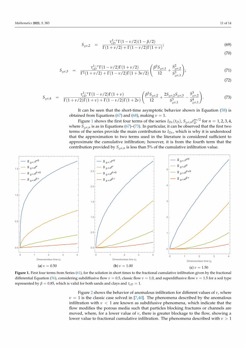
Figure 1 shows the first four terms of the series IDν(tD), SDν,ntnν/2D for n = 1, 2, 3, 4,

where SDν,n is as in Equations (67)–(73). In particular, it can be observed that the first twoterms of the series provide the main contribution to IDν, which is why it is understoodthat the approximation to two terms used in the literature is considered sufficient toapproximate the cumulative infiltration; however, it is from the fourth term that thecontribution provided by SDν,n is less than 5% of the cumulative infiltration value.

(a) ν = 0.50 (b) ν = 1.00 (c) ν = 1.50Figure 1. First four terms from Series (61), for the solution in short times to the fractional cumulative infiltration given by the fractionaldifferential Equation (56), considering subdiffusive flow ν = 0.5, classic flow ν = 1.0, and superdiffusive flow ν = 1.5 for a soil typerepresented by β = 0.85, which is valid for both sands and clays and τcD = 1.

Figure 2 shows the behavior of anomalous infiltration for different values of ν, whereν = 1 is the classic case solved in [7,40]. The phenomena described by the anomalousinfiltration with ν < 1 are known as subdifusive phenomena, which indicate that theflow modifies the porous media such that particles blocking fractures or channels aremoved, where, for a lower value of ν, there is greater blockage to the flow, showing alower value to fractional cumulative infiltration. The phenomena described with ν > 1

Mathematics 2021, 9, 383 12 of 14

is known as superdiffusive phenomena, where the flow modifies the porous media suchthat the particles create new fractures or channels that allow greater mobility to the fluid,where, for a higher value of ν, there is a greater flow and therefore greater fractionalcumulative infiltration.

Figure 2. Short-time-approximated solution given by Series (61) for fractional cumulative infiltrationconsidering subdiffusive flows ν < 1, classical flows ν = 1, and superdiffusive flows ν > 1, for a soiltype represented by β = 0.85 that is valid for sands and clays and τc = 1.

Figure 3 shows the effect of β on the fractional accumulated infiltration IDν(tD) forseveral values of ν. As previously described, β is associated with hydrodynamic charac-teristics of the soil type, where β = 0 corresponds to a linear soil type solved in [1] forν = 1. β = 1 corresponds to the solution given by Talsma and Parlange solved in [6] forν = 1. Further, Figure 3 shows how the effect of ν is greater than β in determining thevalue of the fractional cumulative infiltration IDν; that is, the anomalous soil behavior has agreater impact on the cumulative infiltration compared to the soil type. On the other hand,it can be observed that, for a fixed value of ν, the extreme values of β limit the behavior forcumulative infiltration.

Figure 3. Short-time-approximated solution for fractional cumulative infiltration considering dif-ferent soil types represented by β = 0.0, 0.25, 0.5, 0.75, 1.0, with τcD = 1 and subdiffusive, classical,and superdiffusive flows represented by ν = 0.5, 1.0, 1.5, respectively. Results in green correspondto ν = 1.5, results in orange to ν = 1.0, and results in blue to ν = 0.5, where a more dashed lineindicates a lower value of β.

Mathematics 2021, 9, 383 13 of 14

6. Conclusions

A new model is proposed to capture the phenomenon of anomalous infiltrationthrough the use of fractional calculus considering time t and volumetric water content θas dependent variables and space z as an independent variable. We began the study offractional horizontal infiltration phenomena by neglecting the term associated with thegravitational field, finding as a solution the fractional Boltzmann transform φv and thecorresponding accumulated infiltration. For the study of fractional vertical infiltrationphenomena, the asymptotic solution is found in short and long times for both an arbitrarydiffusivity and hydraulic conductivity; the short-time approximation was expressed asa power series in tν/2, where ν is the order of fractional derivative, and the first termsare expressed as integro-differential equations. Finally, a constant flow–concentrationrelationship and a relation between diffusivity and hydraulic conductivity were consideredto construct a fractional accumulated infiltration model that is valid for all times and fordifferent soil types. The model was solved through a series that was valid for short times.It is shown that the first two terms of the series provide the main contribution to theanomalous infiltration. It is shown that, for subdifusive flows, there is less accumulatedinfiltration than in the classic case; for superdifusive flows, the accumulated infiltrationis greater than the classic case. The effect of considering different types of soils is alsoshown, concluding that, for a fixed value of ν, the extreme values of β limit the behavior ofcumulative infiltration, and the anomalous soil behavior has a greater impact on cumulativeinfiltration compared to the soil type.

Author Contributions: Conceptualization, C.F.; Software, C.F. and F.A.-L.; Supervision, A.Q. andC.C.; Writing—original draft, C.F.; Writing—review & editing, F.A.-L. All authors have read andagreed to the published version of the manuscript.

Funding: The corresponding author of this work is grateful to CONACYT for the scholarship grant,scholarship number 548429.

Institutional Review Board Statement: Not applicable.

Informed Consent Statement: Not applicable.

Data Availability Statement: Not applicable.

Conflicts of Interest: The authors declare no conflict of interest.

References1. Green, W.H.; Ampt, G. Studies on Soil Phyics. J. Agric. Sci. 1911, 4, 1–24. [CrossRef]2. Morbidelli, R.; Corradini, C.; Saltalippi, C.; Flammini, A.; Dari, J.; Govindaraju, R.S. Rainfall infiltration modeling: A review.

Water 2018, 10, 1873. [CrossRef]3. Philip, J.R. Theory of infiltration. Adv. Hydrosci. 1969, 5, 215–296. [CrossRef]4. Boltzmann, L. Zur integration der diffusionsgleichung bei variabeln diffusionscoefficienten. Annalen der Physik 1894, 289, 959–964.

[CrossRef]5. Philip, J. The theory of infiltration: 1. The infiltration equation and its solution. Soil Sci. 1957, 83, 345–358. [CrossRef]6. Talsma, T.; Parlange, J. One dimensional vertical infiltration. Soil Res. 1972, 10, 143–150. [CrossRef]7. Parlange, J.Y.; Lisle, I.; Braddock, R.; Smith, R. The three-parameter infiltration equation. Soil Sci. 1982, 133, 337–341. [CrossRef]8. Haverkamp, R.; Parlange, J.Y.; Starr, J.; Schmitz, G.; Fuentes, C. Infiltration under ponded conditions: 3. A predictive equation

based on physical parameters. Soil Sci. 1990, 149, 292–300. [CrossRef]9. Haverkamp, R.; Kutilek, M.; Parlange, J.Y.; Rendon, L.; Krejca, M. Infiltration under ponded conditions: 2. infiltration equations

tested for parameter time-dependence and predictive use. Soil Sci. 1988, 145, 317–329. [CrossRef]10. Fuentes, C.; Haverkamp, R.; Parlange, J.Y. Parameter constraints on closed-form soilwater relationships. J. Hydrol. 1992,

134, 117–142. [CrossRef]11. Fuentes, C.; Parlange, J.Y.; Haverkamp, R.; Vauclin, M. La solución cuasi-lineal de la infiltración vertical. Tecnología y Ciencias del

Agua 2001, 16, 25–33.12. Saucedo, H.; Fuentes, C.; Zavala, M. El sistema de ecuaciones de Saint-Venant y Richards del riego por gravedad: 3. verificación

numérica de la hipótesis del tiempo de contacto en el riego por melgas. Tecnología y Ciencias del Agua 2006, 21, 135–143.13. Mollerup, M.; Hansen, S. Power series solution for falling head ponded infiltration with evaporation. Water Resour. Res. 2007, 43.

[CrossRef]

Mathematics 2021, 9, 383 14 of 14

14. Mollerup, M. Philip’s infiltration equation for variable-head ponded infiltration. J. Hydrol. 2007, 347, 173–176. [CrossRef]15. Mollerup, M.; Hansen, S. Power series solution for ponded infiltration on sloping surfaces. J. Hydrol. 2012, 464, 431–437.

[CrossRef]16. Peng, Y.; Liu, X.; Zhu, Y.; Yang, Q. Effects of pressure heads and soil bulk density on infiltration characteristics of vertically

inserted moistube irrigation. Environ. Earth Sci. Res. J. 2019, 6, 119–124. [CrossRef]17. Castanedo, V.; Saucedo, H.; Fuentes, C. Modeling Two-Dimensional Infiltration with Constant and Time-Variable Water Depth.

Water 2019, 11, 371. [CrossRef]18. Fuentes, C.; Chávez, C. Analytic Representation of the Optimal Flow for Gravity Irrigation. Water 2020, 12, 2710. [CrossRef]19. Richards, L.A. Capillary conduction of liquids through porous mediums. Physics 1931, 1, 318–333. [CrossRef]20. Holtan, H.N. Concept for Infiltration Estimates in Watershed Engineering; USDA Bulletin: Washington, DC, USA, 1961.21. Sihag, P.; Tiwari, N.; Ranjan, S. Estimation and inter-comparison of infiltration models. Water Sci. 2017, 31, 34–43. [CrossRef]22. Vand, A.S.; Sihag, P.; Singh, B.; Zand, M. Comparative evaluation of infiltration models. KSCE J. Civ. Eng. 2018, 22, 4173–4184.

[CrossRef]23. Timashev, S.F.; Polyakov, Y.S.; Misurkin, P.I.; Lakeev, S.G. Anomalous diffusion as a stochastic component in the dynamics of

complex processes. Phys. Rev. E 2010, 81, 041128. [CrossRef] [PubMed]24. Parlange, J.Y.; Haverkamp, R.; Rand, R.; Rendon, L.; Schmitz, G. Water Movement in Soils-The Role of Analytical Solutions.

Future Dev. Soil Sci. Res. 1978, 11–21. [CrossRef]25. Bhattacharya, R.N.; Gupta, V. On a statistical theory of solute transport in porous media. SIAM J. Appl. Math. 1979, 37, 485–498.

[CrossRef]26. Gorenflo, R.; Mainardi, F.; Vivoli, A. Continuous-time random walk and parametric subordination in fractional diffusion. Chaos

Solitons Fractals 2007, 34, 87–103. [CrossRef]27. Metzler, R.; Klafter, J. The random walk’s guide to anomalous diffusion: a fractional dynamics approach. Phys. Rep. 2000,

339, 1–77. [CrossRef]28. Bagley, R.L. The thermorheologically complex material. Int. J. Eng. Sci. 1991, 29, 797–806. [CrossRef]29. Pachepsky, Y.; Timlin, D.; Rawls, W. Generalized Richards’ equation to simulate water transport in unsaturated soils. J. Hydrol.

2003, 272, 3–13. [CrossRef]30. Sun, H.; Meerschaert, M.M.; Zhang, Y.; Zhu, J.; Chen, W. A fractal Richards’ equation to capture the non-Boltzmann scaling of

water transport in unsaturated media. Adv. Water Resour. 2013, 52, 292–295. [CrossRef]31. Su, N. Theory of infiltration: Infiltration into swelling soils in a material coordinate. J. Hydrol. 2010, 395, 103–108. [CrossRef]32. Su, N. Distributed-order infiltration, absorption and water exchange in mobile and immobile zones of swelling soils. J. Hydrol.

2012, 468, 1–10. [CrossRef]33. Su, N. Mass-time and space-time fractional partial differential equations of water movement in soils: Theoretical framework and

application to infiltration. J. Hydrol. 2014, 519, 1792–1803. [CrossRef]34. Benson, D.A.; Meerschaert, M.M.; Revielle, J. Fractional calculus in hydrologic modeling: A numerical perspective. Adv. Water

Resour. 2013, 51, 479–497. [CrossRef]35. Samko, S.G.; Kilbas, A.A.; Marichev, O.I. Fractional Integrals and Derivatives; Gordon and Breach Science Publishers: Yverdon

Yverdon-les-Bains, Switzerland, 1993; Volume 1.36. Podlubny, I. Fractional Differential Equations: An Introduction to Fractional Derivatives, Fractional Differential Equations, to Methods of

Their Solution and Some of Their Applications; Academic Press: San Diego, CA, USA, 1998.37. Baleanu, D.; Diethelm, K.; Scalas, E.; Trujillo, J.J. Fractional Calculus: Models and Numerical Methods; World Scientific: Singapore,

2012; Volume 3.38. Parlange, J.Y. On solving the flow equation in unsaturated soils by optimization: Horizontal infiltration. Soil Sci. Soc. Am. J. 1975,

39, 415–418. [CrossRef]39. Fuentes, C. Unidimensional infiltration theory: 2. Vertical infiltration. Agrociencia 1989, 78, 119–153.40. Fuentes, C.; Parlange, J.Y.; Palacios-Vélez, O. Infiltration Theory. In Gravity Irrigation, 1st ed.; Fuentes, C.; Rendón, L., Eds.;

National Association of Irrigation Specialists: México, México, 2017; Chapter 3, pp. 154–211.