FRACTIONAL – ORDER FEEDBACK CONTROL OF A DC …iris.elf.stuba.sk/JEEEC/data/pdf/3_109-01.pdf ·...

Journal of ELECTRICAL ENGINEERING, VOL. 60, NO. 3, 2009, 117–128

FRACTIONAL – ORDER FEEDBACK CONTROLOF A DC MOTOR

Ivo Petras∗

This paper deals with the feedback control of a DC motor speed with using the fractional-order controller. The permanent-magnet DC motor is often used in mechatronic and other fields of control theory and therefore its control is very important.The mathematical description of the fractional - order controller and its implementation in the analogue and the discretedomains is presented. An example of simulation and possible realization of the particular case of digital fractional-order

PIλDδ controller are shown as well. The hardware realization is proposed in digital form with the microprocessor and inanalogue form with the fractance circuits.

K e y w o r d s: fractional calculus, fractional-order controller, microprocessor, fractance, DC motor

1 INTRODUCTION

The DC motor is a power actuator, which converts di-rect current electrical energy into rotational mechanicalenergy. The DC motors are still often used in industryand in numerous control applications, robotic manipula-tors and commercial applications such as disk drive, tapemotor as well.

We will consider the armature - controlled DC motorutilizes a constant field current. This kind of the DC mo-tor will be controlled by a nonconventional control tech-nique which is known as a fractional-order control. Men-tioned technique was developed during last few decadesand there are various practical applications as for exam-ple flexible spacecraft attitude control [25], car suspen-sion control [29], temperature control [32], motor control[51], etc. This idea of the fractional calculus applicationto control theory was described in many other works (eg:[4], [15], [31], [38], etc) and its advantages were proved aswell. All these works used the continuous models basedon fractional differential equations or transfer function.For practical application of the fractional-order modelsin control and for realization of the fractional-order con-trollers (FOC), we need discrete fractional-order models.It is also well known that the fractional-order systemshave an unlimited memory (infinite dimensional) whilethe integer-order systems have a limited memory (finitedimensional). It is important to approximately describethe fractional-order systems using a finite difference equa-tions. We will consider new discretization technique pro-posed by Chen et al in [12]. Obtained discrete versionof fractional order controller will be implemented by amicroprocessor and proposed to the DC motor control.

This article is organized as follow: In section 2, wepresent a brief introduction to fractional calculus and itsapproximation. Section 3 presents mathematical modelof DC motor as a controlled object. Section 4 deals with

fractional order control. Section 5 presents some simula-tion results. Section 6 treats of proposal to digital andanalogue realization of the FOC. Section 7 concludes thispaper by some remarks and conclusions.

2 FUNDAMENTALS OF

FRACTIONAL CALCULUS

2.1 A bit of history and definitions

Fractional calculus is a generalization of integrationand differentiation to non-integer (fractional) order fun-damental operator aDr

t , where a and t are the limits and(r ∈ R) is the order of the operation. There are severaldefinition of fractional integration and differentiation (see[28], [29], [39]). The most often used are the Grunwald-Letnikov (GL) definition and the Riemann-Liuville defi-nition (RL). For a wide class of functions, the two defini-tions – GL and RL – are equivalent [39].

The GL is given as

aDrt f(t) = lim

h→0h−r

[ t−a

h]∑

j=0

(−1)j

(r

j

)f(t − jh), (1)

where [·] means the integer part. The RL definition isgiven as

aDrt f(t) =

1

Γ(n − r)

dn

dtn

∫ t

a

f(τ)

(t − τ)r−n+1dτ , (2)

for (n − 1 < r < n) and where Γ(·) is the Gamma

function.

For many engineering applications the Laplace trans-form methods are often used. The Laplace transform ofthe GL and RL fractional derivative/integral, under zeroinitial conditions for order r is given by [28]:

L- aD±rt f(t); s = s±rF (s) . (3)

∗ Institute of Control and Informatization of Production Processes, Faculty of BERG, Technical University of Kosice, B. Nemcovej 3,042 00 Kosice, Slovakia, [email protected]

ISSN 1335-3632 c© 2009 FEI STU

118 I. Petras: FRACTIONAL - ORDER FEEDBACK CONTROL OF A DC MOTOR

Fig. 1. Bode’s ideal loop

Fig. 2. Bode plots of transfer function Go(s) in (5)

Some other important properties of the fractionalderivatives and integrals can be found in several works([28],[ 29], [39], etc).

Geometric and physical interpretation of fractional in-tegration and fractional differentiation were exactly de-scribed in [40].

2.2 Bode’s ideal loop as a reference model

H. W. Bode suggested an ideal shape of the loop trans-fer function in his work on design of feedback amplifiersin 1945. Ideal loop transfer function has form [7]:

L(s) =( s

ωgc

)α

, (4)

where ωgc is desired crossover frequency and α is slopeof the ideal cut-off characteristic.

Phase margin is Φm = π(1+α/2) for all values of thegain. The amplitude margin Am is infinity. The constantphase margin 60o , 45o and 30o correspond to the slopesα = −1.33, −1.5 and −1.66.

The Nyquist curve for ideal Bode transfer function issimply a straight line through the origin witharg(L(jω)) = απ/2.

Bode’s transfer function (4) can be used as a referencesystem in the following form [3], [24], [36], [41], [50]:

Gc(s) =K

sα + K, Go(s) =

K

sα, (0 < α < 2), (5)

where Gc(s) is transfer function of closed loop and Go(s)is transfer function in open loop.

General characteristics of Bode’s ideal transfer func-tion are:

(a) Open loop:

• Magnitude: constant slope of −α20 dB/dec;

• Crossover frequency: a function of K;

• Phase: horizontal line of −απ2 ;

• Nyquist: straight line at argument −απ2 .

(b) Closed loop:

• Gain margin: Am = ∞ ;

• Phase margin: constant : Φm = π(1 − α

2

);

• Step response:

y(t) = KtαEα,α+1 (−Ktα) ,

where Ea,b(z) is the Mittag-Leffler function of twoparameters [38].

2.3 Continuous time approximation of fractional

calculus

A detailed review of the various approximation meth-ods and techniques for continuous and discrete fractional-order models in form of IIR and FIR filters was done inwork [45].

For simulation purpose, here we present the Oustaloup’sapproximation algorithm [29], [30]. The method is basedon the approximation of a function of the form:

H(s) = sr, r ∈ R, r ∈ [−1; 1] (6)

for the frequency range selected as (ωb, ωh) by a rationalfunction:

H(s) = Co

N∏

k=−N

s + ω′k

s + ωk

(7)

using the following set of synthesis formulas for zeros,poles and the gain:

ω′

k = ωb

(ωh

ωb

) k+N+0.5(1−r)2N+1

,

ωk = ωb

(ωh

ωb

) k+N+0.5(1−r)2N+1

, (8)

Co =(ωh

ωb

)−r

2N∏

k=−N

ωk

ω′

k

, (9)

where ωh, ωb are the high and low transitional frequen-cies. An implementation of this algorithm in Matlab as afunction script ora foc() is given in [14].

Using the described Oustaloup-Recursive-Approxi-mation (ORA) method with:

ωh = 103, ωb = 10−3, (10)

the obtained approximation for fractional function

H(s) = s−12 is:

H5(s) =

s5 + 74.97s4 + 768.5s3 + 1218s2 + 298.5s + 10

10s5 + 298.5s4 + 1218s3 + 768.5s2 + 74.97s + 1. (11)

The Bode plots and the unit step response of the ap-proximated fractional order integrator (11) are depictedin Fig. 3. Bode plots can be compared with the ideal plotsdepicted in Fig. 2.

Journal of ELECTRICAL ENGINEERING 60, NO. 3, 2009 119

Fig. 3. Characteristics of approximated fractional order integrator (11): Bode plots for r = −0.5 and N = 5 (left), Unit step responsefor r = −0.5 and N = 5 (right)

2.4 Discrete time approximation of fractional

calculus

In general, the discretization of fractional-order differ-entiator/integrator s±r (r ∈ R) can be expressed by the

so-called generating function s ≈ ω(z−1). This generat-ing function and its expansion determine both the formof the approximation and the coefficients [19].

As a generating function ω(z−1) can be used in gen-erally the following formula [6]:

ω(z−1) =( 1

βT

1 − z−1

γ + (1 − γ)z−1

), (12)

where β and γ are denoted the gain and phase tuningparameters, respectively. For example, when β = 1 andγ = 0, 1/2, 7/8, 1, 3/2 , the generating function (12)becomes the forward Euler, the Tustin, the Al-Alaoui, thebackward Euler, the implicit Adams rules, respectively. Inthis sense the generating formula can be tuned precisely.

The expansion of the generating functions can be doneby Power Series Expansion (PSE) or Continued FractionExpansion (CFE).

It is very important to note that PSE scheme leads toapproximations in the form of polynomials, that is, thediscretized fractional order derivative is in the form ofFIR filters, which have only zeros.

Taking into account that our aim is to obtain discreteequivalents to the fractional integrodifferential operatorsin the Laplace domain, s±r , the following considerationshave to be made [46]:

1. sr , (0 < r < 1), viewed as an operator, has a branchcut along the negative real axis for arguments of s on(−π, π) but is free of poles and zeros.

2. It is well known that, for interpolation or evaluationpurposes, rational functions are sometimes superior topolynomials, roughly speaking, because of their abil-ity to model functions with zeros and poles. In otherwords, for evaluation purposes, rational approxima-tions frequently converge much more rapidly than PSE

and have a wider domain of convergence in the com-plex plane.

In this paper, for directly discretizing sr , (0 < r < 1),we shall concentrate on the IIR form of discretizationwhere as a generating function we will adopt an Al-Alaouiidea on mixed scheme of Euler and Tustin operators [1],[2] but we will use a different ration between both oper-ators. The mentioned new operator, raised to power ±r ,has the form [34]:

(ω(z−1))±r =(1 + a

T

1 − z−1

1 + az−1

)±r

, (13)

where a is ratio term and r is fractional order. The ratioterm a is the amount of phase shift and this tuning knobis sufficient for most solved engineering problems.

In expanding the above in rational functions, we willuse the CFE. It should be pointed out that, for controlapplications, the obtained approximate discrete-time ra-tional transfer function should be stable and minimumphase. Furthermore, for a better fit to the continuous fre-quency response, it would be of high interest to obtaindiscrete approximations with poles an zeros interlacedalong the line z ∈ (−1, 1) of the z plane. The direct dis-cretization approximations proposed in this paper enjoythe desirable properties.

The result of such approximation for an irrational

function, G(z−1), can be expressed by G(z−1) in theCFE form [46]:

G(z−1) ≃

a0(z−1) +

b1(z−1)

a1(z−1) + b2(z−1)

a2(z−1)+b3(z−1)

a3(z−1)+...

= a0(z−1) +

b1(z−1)

a1(z−1)+

b2(z−1)

a2(z−1)+. . .

b3(z−1)

a3(z−1)+. . .

(14)

where ai and bi are either rational functions of the vari-able z−1 or constants. The application of the method


Fig. 4. Characteristics of approximated fractional order differentiator (16): Bode plots for r = 0.5, n = 5, a = 1/3, and T = 0.001 s in(15) (left), Unit step responses for r = 0.5, n = 5, a = 1/3, and T = 0.001 s in (15) (right)

Fig. 5. Characteristics of approximated fractional order integrator (17): Bode plots for r = −0.5, n = 5, a = 1/3, and T = 0.001 s in(15) (left), Unit step responses for r = −0.5, n = 5, a = 1/3, and T = 0.001 s in (15) (right)

yields a rational function, G(z−1), which is an approxi-

mation of the irrational function G(z−1).

The resulting discrete transfer function, approximat-

ing fractional-order operators, can be expressed as:

(ω(z−1))±r ≈(1 + a

T

)±r

CFE( 1 − z−1

1 + az−1

)±r

p,q

=(1 + a

T

)±r Pp(z−1)

Qq(z−1), (15)

=(1 + a

T

)±r p0 + p1z−1 + · · · + pmz−p

q0 + q1z−1 + · · · + qnz−q,

where CFEu denotes the continued fraction expansion

of u ; p and q are the orders of the approximation and

P and Q are polynomials of degrees p and q . Normally,

we can set p = q = n .

In Matlab Symbolic Toolbox, by the following script,

for a given n we can easily get the approximated direct

discretization of fractional order derivative (let us denote

that x = z−1 ):

syms r a x;maple(’with(numtheory)’);

f = ((1-x)/(1+a*x))^r;;

n=5; n2=2*n;

maple([’cfe := cfrac(’ char(f) ’,x,n2);’])

pq=maple(’P over Q := nthconver’,’cfe’,n2)

p0=maple(’P := nthnumer’,’cfe’,n2)

q0=maple(’Q := nthdenom’,’cfe’,n2)

p=(p0(5:length(p0)));q=(q0(5:length(q0)));

p1=collect(sym(p),x)

q1=collect(sym(q),x)

Modified and improved digital fractional-order differen-tiator using fractional sample delay and digital integratorusing recursive Romberg integration rule and fractionalorder delay as well has been described in [42].

Some others solutions for design IIR approximation us-ing least-squares eg: the Pade approximation, the Prony’smethod and the Shranks’ method were described in [6].The Prony and Shranks methods can produce better ap-proximations the widely used CFE method. The Pade andthe CFE methods yield the same approximation (causal,


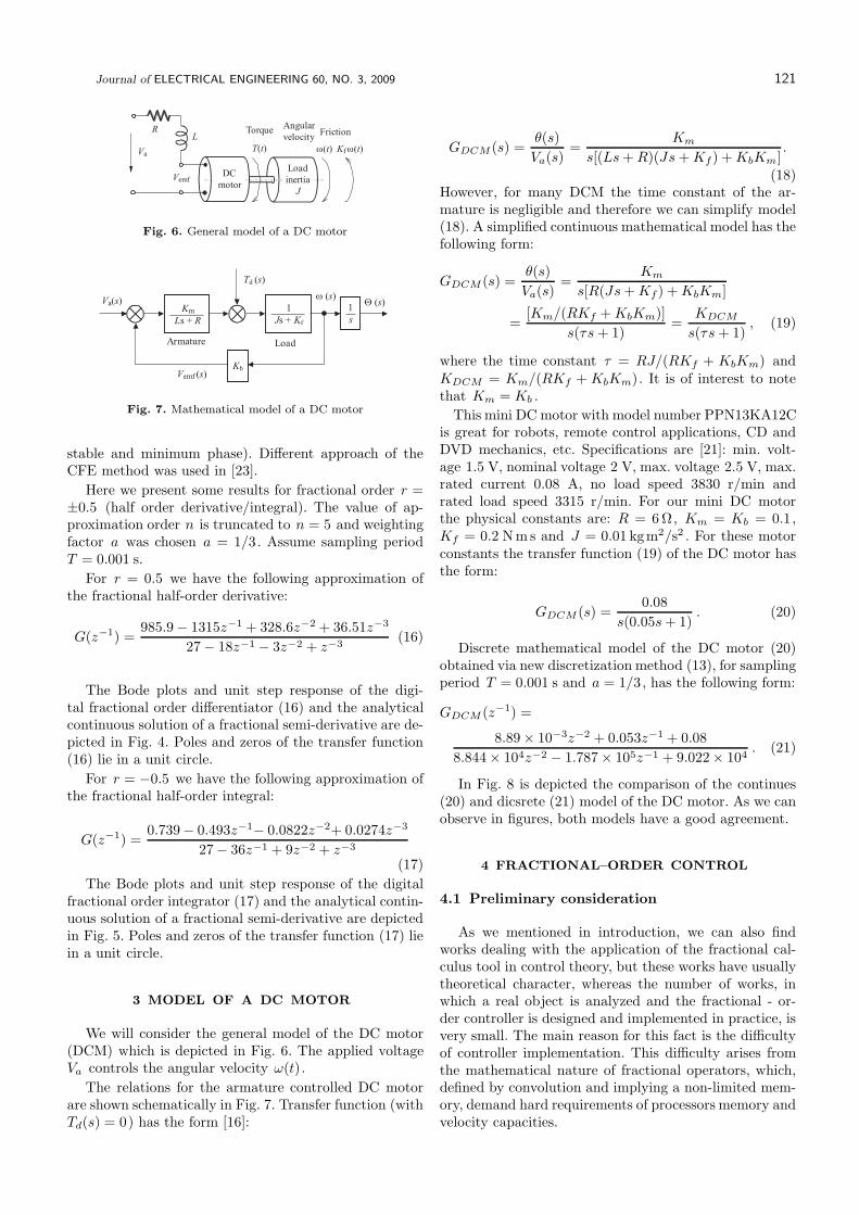
Fig. 6. General model of a DC motor

Fig. 7. Mathematical model of a DC motor

stable and minimum phase). Different approach of theCFE method was used in [23].

Here we present some results for fractional order r =±0.5 (half order derivative/integral). The value of ap-proximation order n is truncated to n = 5 and weightingfactor a was chosen a = 1/3. Assume sampling periodT = 0.001 s.

For r = 0.5 we have the following approximation ofthe fractional half-order derivative:

G(z−1) =985.9 − 1315z−1 + 328.6z−2 + 36.51z−3

27 − 18z−1 − 3z−2 + z−3(16)

The Bode plots and unit step response of the digi-tal fractional order differentiator (16) and the analyticalcontinuous solution of a fractional semi-derivative are de-picted in Fig. 4. Poles and zeros of the transfer function(16) lie in a unit circle.

For r = −0.5 we have the following approximation ofthe fractional half-order integral:

G(z−1) =0.739− 0.493z−1− 0.0822z−2+ 0.0274z−3

27 − 36z−1 + 9z−2 + z−3

(17)

The Bode plots and unit step response of the digitalfractional order integrator (17) and the analytical contin-uous solution of a fractional semi-derivative are depictedin Fig. 5. Poles and zeros of the transfer function (17) liein a unit circle.

3 MODEL OF A DC MOTOR

We will consider the general model of the DC motor(DCM) which is depicted in Fig. 6. The applied voltageVa controls the angular velocity ω(t).

The relations for the armature controlled DC motorare shown schematically in Fig. 7. Transfer function (withTd(s) = 0) has the form [16]:

GDCM (s) =θ(s)

Va(s)=

Km

s[(Ls + R)(Js + Kf) + KbKm].

(18)However, for many DCM the time constant of the ar-mature is negligible and therefore we can simplify model(18). A simplified continuous mathematical model has thefollowing form:

GDCM (s) =θ(s)

Va(s)=

Km

s[R(Js + Kf) + KbKm]

=[Km/(RKf + KbKm)]

s(τs + 1)=

KDCM

s(τs + 1), (19)

where the time constant τ = RJ/(RKf + KbKm) andKDCM = Km/(RKf + KbKm). It is of interest to notethat Km = Kb .

This mini DC motor with model number PPN13KA12Cis great for robots, remote control applications, CD andDVD mechanics, etc. Specifications are [21]: min. volt-age 1.5 V, nominal voltage 2 V, max. voltage 2.5 V, max.rated current 0.08 A, no load speed 3830 r/min andrated load speed 3315 r/min. For our mini DC motorthe physical constants are: R = 6 Ω, Km = Kb = 0.1,Kf = 0.2 Nms and J = 0.01 kgm2/s2 . For these motorconstants the transfer function (19) of the DC motor hasthe form:

GDCM (s) =0.08

s(0.05s + 1). (20)

Discrete mathematical model of the DC motor (20)obtained via new discretization method (13), for samplingperiod T = 0.001 s and a = 1/3, has the following form:

GDCM (z−1) =

8.89 × 10−3z−2 + 0.053z−1 + 0.08

8.844 × 104z−2 − 1.787 × 105z−1 + 9.022× 104. (21)

In Fig. 8 is depicted the comparison of the continues(20) and dicsrete (21) model of the DC motor. As we canobserve in figures, both models have a good agreement.

4 FRACTIONAL–ORDER CONTROL

4.1 Preliminary consideration

As we mentioned in introduction, we can also findworks dealing with the application of the fractional cal-culus tool in control theory, but these works have usuallytheoretical character, whereas the number of works, inwhich a real object is analyzed and the fractional - or-der controller is designed and implemented in practice, isvery small. The main reason for this fact is the difficultyof controller implementation. This difficulty arises fromthe mathematical nature of fractional operators, which,defined by convolution and implying a non-limited mem-ory, demand hard requirements of processors memory andvelocity capacities.


Fig. 8. Comparison of characteristics for both models of a DC motor: Bode plots of the motor models (left), Comparison of characteristicsfor both models of a DC motor (right)

Fig. 9. Feedback control loop

4.2 Fractional-order controllers

The fractional-order PIλDδ controller was proposedas a generalization of the PID controller with integratorof real order λ and differentiator of real order δ . Thetransfer function of such type the controller in Laplacedomain has form [38]:

C(s) =U(s)

E(s)= Kp + Ki s−λ + Kd sδ, (λ, δ > 0) , (22)

where Kp is the proportional constant, Ki is the inte-gration constant and Kd is the differentiation constant.

Transfer function (22) corresponds in discrete domainwith the discrete transfer function in the following ex-pression [46]:

C(z−1) =U(z−1)

E(z−1)= Kp + Ki(ω(z−1))−λ+ Kd(ω(z−1))δ,

(23)where λ and δ are arbitrary real numbers.

Taking λ = 1 and δ = 1, we obtain a classical PIDcontroller. If δ = 0 and Kd = 0, we obtain a PIλ

controller, etc. All these types of controllers are particular

cases of the PIλDδ controller, which is more flexibleand gives an opportunity to better adjust the dynamicalproperties of the fractional-order control system.

There are many another considerations of the frac-tional-order controller. For example we can notice theCRONE controller [29], the non-integer integral and itsapplication to control [24] or the TID compensator [20],

which has a similar structure as a PID controller but the

proportional component is replaced with a tilted compo-

nent having a transfer function s to the power of (−1/n).

All those fractional-order controllers are sometimes

called optimal phase controllers because only with non-

integer order we can get a constant phase somewhere be-

tween 0o and −180o depending on the parameters λ and

δ .

4.3 Fractional-order controller design

For the FOC design we will use an idea which was

proposed by Bode [7] and for first time used to the motion

control described by Tustin [43]. This principle was also

used by Manabe to induction motor speed control [25].

The several methods and tuning techniques for the

FOC parameters were developed during the past ten

years. They are based on various approaches (see [5], [13],

[22], [26], [31], [49], [52]).

In Fig. 9 is depicted feedback control loop, where C(s)

is transfer function of controller and GDCM (s) is transfer

function of the DC motor.

We will design the controller, which give us a step re-

sponse of feedback control loop with overshoot indepen-

dent of payload changes (iso-damping). In the frequency

domain point of view it means phase margin independent

of the payload changes.

Phase margin of controlled system is [9], [48]

Φm = arg [C(jωg)GDCM (jωg)] + π , (24)

where jωg is the crossover frequency. Independent phase

margin means in other words constant phase. This can

be accomplished by controller of the form

C(s) = k1k2s + 1

sµ, k1 = 1/KDCM , k2 = τ . (25)


Fig. 10. Characteristics of fractional order transfer function (28): Bode plots – continuous and discrete models n = 5, a = 1/3, andT = 0.1 s (left), Unit step responses –continuous and discrete models n = 5, a = 1/3, and T = 0.1 s (right)

Fig. 11. Simulink block nipid - fractional order controller

Fig. 12. Simulink model for feedback control of the DC motor

Such controller gives a constant phase margin and ob-tained phase margin is

Φm = arg [C(jω)GDCM (jω)] + π

= arg

[k1KDCM

(jω)(1+µ)

]+ π

= arg[(jω)−(1+µ)

]+ π = π − (1 + µ)

π

2. (26)

For our parameters of controlled object (20) and de-sired phase margin Φm = 45o , we get the following con-stants of the fractional order controllres (25): k1 = 12.5,k2 = 0.05 and µ = 0.5. With these constants we obtain

a fractional IλDδ controller, which is a particular case ofthe PIλDδ controller and has the form

C(s) =τ

KDCM

s0.5 +1

KDCMs0.5

= Kds0.5 + Kis

−0.5 = 0.625√

s +12.5√

s, (27)

where Ki = 12.5, Kd = 0.625 and δ = λ = 0.5.

According to relation (26), by using a controller (27),we can obtain a phase margin

Φm = arg [C(jω)GDCM (jω)] + π = π − (1.5)π

2= 45,

which was desired phase margin specification.

5 SIMULATION RESULTS

The transfer function of the closed feedback controlloop with the fractional-order controller (27) and the DCmotor (20) has the following form:

Gc(s) =Go(s)

1 + Go(s)=

GDCM (s)C(s)

1 + GDCM (s)C(s)

=0.05s + 1

0.05s2.5 + s1.5 + 0.05s + 1, (28)

where Go(s) is the transfer function of the open controlloop with

Go(s) =0.05s + 1

0.05s2.5 + s1.5.

The feedback control loop described above can be sim-ulated in Matlab environment with using the approxima-tion technique described before, namely Oustaloup’s re-


Fig. 13. Comparison of unit step responses of a feedback control loop: Unit step response without actuator saturation overshoot ≈ 30%,set. time ≈ 11 s (left), Unit step response with actuator saturation overshoot ≈ 40 %, settling time ≈ 14 s (right)

cursive approximation function ora foc() for the desiredfrequency range given in (10).

close all; clear all;

Gs DCM=tf([0.08],[0.05 1 0]);

Cs=(0.625*ora foc(0.5,6,0.001,1000))

+(12.5*ora foc(-0.5,6,0.001,1000));

Gs close=(Gs DCM*Cs)/(1+(Gs DCM*Cs));

step(Gs close,15);

Gs open=(Gs DCM*Cs);

bode(Gs open);

[Gm,Pm] = margin(Gs open);

The results obtained via described Matlab scripts aredepicted in Fig. 10. Continues model is shown with solidline. Phase margin is Φm ≈ 44.9 and gain margin isinfinite.

The disrete version of the continues fractional ordertransfer function can be obtained with using the digitaloperator (13) and Matlab function for approximation ofdigital fractional order derivative/integral dfod1(). As-sume that T = 0.1 s and a = 1/3.

close all; clear all;

T=0.1;

a=1/3;

z=tf(’z’,T,’variable’,’z^-1’)

Hz=((1+a)/T)*((1-z^-1)/(1+a*z^-1));

Gz DCM=0.08/(Hz*(0.05*Hz+1));

Cz=0.625*dfod1(5,T,a,0.5)+12.5*dfod1(5,T,a,-0.5);

Gz close=(Gz DCM*Cz)/(1+(Gz DCM*Cz));

step(Gz close,15);

Gz open=(Gz DCM*Cz);

bode(Gz open);

[Gm,Pm] = margin(Gz open);

The results obtained via described Matlab scripts aredepicted in Fig. 10. Discrete model is shown with dashedline. Phase margin is Φm ≈ 45.1 and gain margin isinfinite.

Simulation of the closed feedback loop can also bedome in Matlab/Simulink environment, where fractional- order controller is realized via nipid block proposed by

D. Valerio [44], where block parameters are depicted inFig. 11.

General Simulink model is shown in Fig. 12. Blockconstants were set according to parameters of DC motorand fractional-order controller.

Time domain simulation results for fractional orderfeedback loop are depicted in Fig. 13. Obtained resultsare comparable with the results obtained with simulationin Matlab by routines.

Stability analysis is investigated by solving the char-acteristic equation of transfer function (28) with usingMatlab function solve()

s=solve(’0.05*s^2.5 + s^1.5 + 0.05*s + 1 = 0’,’s’)

with the following results: s1,2 = −0.5 ± 0.86602j ands3 = −20. It means that feedback control loop is stable.

As we can observe in Fig. 13, the quality indexes (over-shoot and settling time) are worse in the case of controlloop with saturation, because of controller power limita-tions.

Fig. 14. Actuator for the DC motor

6 PROPOSED REALIZATIONS OF FOC

Basically, there are two methods for realization of theFOC. One is a digital realization based on processor de-vices and appropriate control algorithm and the second


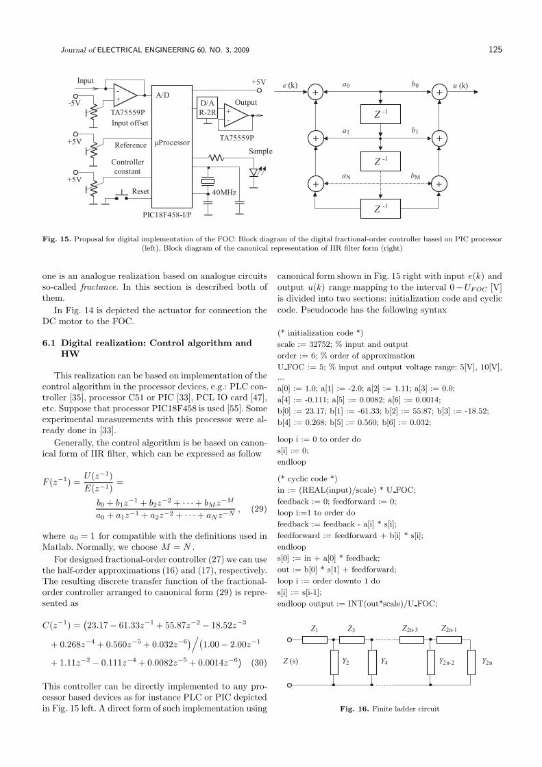
Fig. 15. Proposal for digital implementation of the FOC: Block diagram of the digital fractional-order controller based on PIC processor(left), Block diagram of the canonical representation of IIR filter form (right)

one is an analogue realization based on analogue circuitsso-called fractance. In this section is described both ofthem.

In Fig. 14 is depicted the actuator for connection theDC motor to the FOC.

6.1 Digital realization: Control algorithm and

HW

This realization can be based on implementation of thecontrol algorithm in the processor devices, e.g.: PLC con-troller [35], processor C51 or PIC [33], PCL IO card [47],etc. Suppose that processor PIC18F458 is used [55]. Someexperimental measurements with this processor were al-ready done in [33].

Generally, the control algorithm is be based on canon-ical form of IIR filter, which can be expressed as follow

F (z−1) =U(z−1)

E(z−1)=

b0 + b1z−1 + b2z

−2 + · · · + bMz−M

a0 + a1z−1 + a2z−2 + · · · + aNz−N, (29)

where a0 = 1 for compatible with the definitions used inMatlab. Normally, we choose M = N .

For designed fractional-order controller (27) we can usethe half-order approximations (16) and (17), respectively.The resulting discrete transfer function of the fractional-order controller arranged to canonical form (29) is repre-sented as

C(z−1) =(23.17 − 61.33z−1 + 55.87z−2 − 18.52z−3

+ 0.268z−4 + 0.560z−5 + 0.032z−6)/(

1.00 − 2.00z−1

+ 1.11z−2 − 0.111z−4 + 0.0082z−5 + 0.0014z−6)

(30)

This controller can be directly implemented to any pro-cessor based devices as for instance PLC or PIC depictedin Fig. 15 left. A direct form of such implementation using

canonical form shown in Fig. 15 right with input e(k) andoutput u(k) range mapping to the interval 0−UFOC [V]is divided into two sections: initialization code and cyclic

code. Pseudocode has the following syntax

(* initialization code *)

scale := 32752; % input and output

order := 6; % order of approximation

U FOC := 5; % input and output voltage range: 5[V], 10[V],...

a[0] := 1.0; a[1] := -2.0; a[2] := 1.11; a[3] := 0.0;

a[4] := -0.111; a[5] := 0.0082; a[6] := 0.0014;

b[0] := 23.17; b[1] := -61.33; b[2] := 55.87; b[3] := -18.52;

b[4] := 0.268; b[5] := 0.560; b[6] := 0.032;

loop i := 0 to order do

s[i] := 0;

endloop

(* cyclic code *)

in := (REAL(input)/scale) * U FOC;

feedback := 0; feedforward := 0;

loop i:=1 to order do

feedback := feedback - a[i] * s[i];

feedforward := feedforward + b[i] * s[i];

endloop

s[0] := in + a[0] * feedback;

out := b[0] * s[1] + feedforward;

loop i := order downto 1 do

s[i] := s[i-1];

endloop output := INT(out*scale)/U FOC;

Fig. 16. Finite ladder circuit


Fig. 17. Analogue fractional-order PIλDδ controller

The disadvantage with this solution is that the com-plete controller is calculated using floating point arith-metic.

There are many softwares for PIC programming. Asfor example: Microchip MPLAB, HiTech C Compiler,PICBasic Pro, etc.

6.2 Analogue realization: Fractance circuits and

fractor

A circuit exhibiting fractional-order behavior is calleda fractance [39]. The fractance devices have the follow-ing characteristics [27], [28], [18]. First the phase angleis constant independent of the frequency within a widefrequency band. Second it is possible to construct a fil-ter which has moderated characteristics which can not berealized by using the conventional devices.

Generally speaking, there are three basic fractance de-vices. The most popular is a domino ladder circuit net-work. Very often used is a tree structure of electrical ele-ments and finally, we can find out also some transmissionline circuit. Here we must mention that all basic electricalelements (resistor, capacitor and coil) are not ideal [10],[54].

Design of fractances can be done easily using any of therational approximations [36] or a truncated CFE, whichalso gives a rational approximation.

Truncated CFE does not require any further trans-formation; a rational approximation based on any othermethods must be transformed to the form of a continuedfraction. The values of the electric elements, which arenecessary for building a fractance, are then determinedfrom the obtained finite continued fraction. If all coeffi-cients of the obtained finite continued fraction are posi-tive, then the fractance can be made of classical passiveelements (resistors and capacitors). If some of the coeffi-cients are negative, then the fractance can be made withthe help of negative impedance converters [37].

Domino ladder lattice networks can approximate frac-tional operator more effectively than the lumped net-works [17].

Let us consider the circuit depicted in Fig. 16, whereZ2k−1(s) and Y2k(s), k = 1, . . . , n , are given impedancesof the circuit elements. The resulting impedance Z(s) ofthe entire circuit can be found easily, if we consider it inthe right-to-left direction:

Z(s) = Z1(s)+

1

Y2(s) +1

Z3(s) +1

Y4(s) +

1. . . . . . . . . . . . . . . . . . . . . . . . . . . . .

1

Y2n−2(s) +1

Z2n−1(s) +1

Y2n(s)

(31)

The relationship between the finite domino ladder net-work, shown in Fig. 16, and the continued fraction (31)provides an easy method for designing a circuit witha given impedance Z(s). For this one has to obtaina continued fraction expansion for Z(s). Then the ob-tained particular expressions for Z2k−1(s) and Y2k(s),k = 1, . . . , n , will give the types of necessary componentsof the circuit and their nominal values.

Rational approximation of the fractional integrator/differentiator can be formally expressed as

s±α ≈ Pp(s)

Qq(s)

p,q= Z(s) , (32)

where p and q are the orders of the rational approxi-mation, P and Q are polynomials of degree p and q ,respectively.

For direct calculation of circuit elements was proposedmethod by Wang [53]. This method was designed for con-structing resistive-capacitive ladder network and trans-mission lines that have a generalized Warburg impedanceAs−α , where A is independent of the angular frequencyand 0 < α < 1. This impedance may appear at an elec-trode/electrolyte interface, etc. The impedance of the lad-der network (or transmission line) can be evaluated andrewritten as a continued fraction expansion:

Z(s) = R0 +1

C0s+

1

R1+

1

C1s+

1

R2+

1

C2s+. . . (33)

If we consider that Z2k−1 ≡ Rk−1 and Y2k ≡ Ck−1 fork = 1, . . . , n in Fig. 16, then the values of the resistorsand capacitors of the network are specified by

Rk = 2hαP (α)Γ(k + α)

Γ(k + 1 − α)− hαδko

Ck = h1−α(2k + 1)Γ(k + 1 − α)

P (α)Γ(k + 1 + α),

P (α) =Γ(1 − α)

Γ(α),

(34)

where 0 < α < 1, h is an arbitrary small number, δko isthe Kronecker delta, and k is an integer, k ∈ [0,∞).


In Fig. 17 is depicted an analogue implementation offractional-order PIλDδ controller. Fractional order dif-ferentiator is approximated by general Warburg impedan-ce Z(s)d and fractional order integrator is approximatedby impedance Z(s)i , where orders of both approxima-tions are 0 < α < 1. For orders greater than 1, the War-burg impedance can be combined with classical integerorder one. Usually we suppose R2 = R1 in Fig. 17. Forproportional gain Kp we can write the formula

Kp =R3

R4.

The integration and derivation constants Ki and Kd canbe computed from relationships

Ki =Z(s)i

Ri

, Kd =Rd

Z(s)d

.

In the case, if we use identical resistors (R -series) andidentical capacitors (C -shunt) in the fractances, then thebehavior of the circuit will be as a half-order integra-tor/differentiator. Realization and measurements of suchkind controllers were done in [36]. Some others experi-mental results we can find in [11].

Instead fractance circuit the new electrical elementintroduced by G. Bohannan which is so-called fractor canbe used as well [8]. This element — fractor made from amaterial with the properties of LiN2 H5 SO4 has beenalready used for temperature control [5].

7 CONCLUSION

In this paper was presented a case study of frac-tional order feedback control of a DC motor. Describedmethod is based on Bode’s ideal control loop. Designalgorithm for fractional-order PIλDδ controller param-eters uses a phase margin specification of open con-trol loop. Another very important advantage is an iso-damping property of such control loop. Simulation resultsobtained via Matlab/Simulink confirm the described the-oretical suggestion. This article also proposed digital andanalogue realization of fractional-order controller. De-scribed techniques are useful for practical implementationof fractional-order controllers as the non-conventionalcontrol techniques. However this approach also gave agood start for analysis and design of the analog fractionalorder controller. The fractional-order controller gives usan insight into the concept of memory of the fractionalorder operator. The design, realization, and implementa-tion of the fractional order control systems also becamepossible and much easier than before.

Acknowledgment

This work was supported in part by the Slovak GrantAgency for Science under grants VEGA: 1/4058/07,1/0365/08 and 1/0404/08, and grant APVV-0040-07.

References

[1] Al-ALAOUI, M. A. : Novel Digital Integrator and Differentiator,

Electron. Lett. 29 No. 4 (1993), 376-378.

[2] Al-ALAOUI, M. A. : Filling the Gap between the Bilinear and

the Backward Difference Transforms: An Interactive Design Ap-

proach, Int. J. Elect. Eng. Edu. 34 No. 4 (1997), 331-337.

[3] ASTROM, K. J. : Model Uncertainty and Robust Control,

COSY project, 2000.

[4] AXTELL, M.—BISE, E. M. : Fractional Calculus Applications

in Control Systems, Proc. of the IEEE 1990 Nat. Aerospace and

Electronics Conf, New York, 1990, pp. 563–566.

[5] BASHKARAN, T.—CHEN, Y. Q.—BOHANNAN, G. : Practi-

cal Tuning of Fractional Order Proportional and Integral Con-

troller (II): Experiments, Proc. of the ASME 2007 International

Design Engineering Technical Conferences & Computers and In-

formation in Engineering Conference, Las Vegas, Nevada, USA,

September 4-7, 2007.

[6] BARBOSA, R. S.—MACHADO, J. A. T.—SILVA, M. F. :

Time Domain Design of Fractional Differintegrators using Least-

Squares, Signal Processing 86 (2006), 2567–2581.

[7] BODE, H. W. : Network Analysis and Feedback Amplifier De-

sign, Tung Hwa Book Company, 1949.

[8] BOHANNAN, G. : Analog Realization of a Fractional Control

Element – Revisited, Proc. of the 41st IEEE Int. Conf. on De-

cision and Control, Tutorial Workshop 2: Fractional Calculus

Applications in Automatic Control and Robotics, Las Vegas,

USA, December 9, 2002.

[9] BIDAN, P. : Commande diffusive d’une machine electrique:

une introduction, ESAIM Proceedings, vol. 5, France, 1998,

pp. 55–68.

[10] CARLSON, G. E.—HALIJAK, C. A. : Approximation of Frac-

tional Capacitors (1/s)1/n by a Regular Newton Process, IEEE

Trans. on Circuit Theory 11 No. 2 (1964), 210–213.

[11] CHAREF, A. : Analogue Realisation of Fractional-Order Inte-

grator, Differentiator and Fractional PIIDm Controller, IEEE

Proc.-Control Theory Appl. 153 No. 6 (Nov 2006), 714–720.

[12] CHEN, Y. Q.—MOORE, K. L. : Discretization Schemes for

Fractional-Order Differentiators and Integrators, IEEE Trans.

On Circuits and Systems - I: Fundamental Theory and Applica-

tions .49 No. 3 (2002), 363–367.

[13] CHEN, Y. Q. : Tuning Method for Fractional-Order Controllers,

United States Patent, US2006/0265085 A1, USA, 2006.

[14] CHEN, Y. Q. : Oustaloup-Recursive-Approximation for Frac-

tional Order Differentiators, MathWorks Inc, August 2003:

http://www.mathworks.com/matlabcentral/fileexchange/3802.

[15] DORCAK, L. : Numerical Models for Simulation the Frac-

tional-Order Control Systems, UEF-04-94, Slovak Acad. Sci.,

Kosice, 1994.

[16] DORF, R. C.—BISHOP, R. H. : Modern Control Systems, Ad-

dison-Wesley, New York, 1990.

[17] DUTTA ROY, S. C. : On the Realization of a Constant-Argu-

ment Immitance of Fractional Operator, IEEE Transactions on

Circuit Theory 14 No. 3 (1967), 264–374.

[18] ICHISE, M.—NAGAYANAGI, Y.—KOJIMA, T. : An Analog

Simulation of Non-Integer Order Transfer Functions for Anal-

ysis of Electrode Processes, J. Electroanal. Chem. 33 (1971),

253–265.

[19] LUBICH, C. : Discretized Fractional Calculus, SIAM J. Math.

Anal. 17 No. 3 (1986), 704–719.

[20] LURIE, B. J. : Three-Parameter Tunable Tilt-Integral-Deriva-

tive (TID) Controller, United States Patent, 5 371 670, USA,

1994.

[21] Manual for DC motor PPN13: Minebea Motor Manufacturing

Corporation, http://www.eMinebea.com/.


[22] MACHADO, J. A. T. : Analysis and Design of Fractional-OrderDigital Control Systems, J. Syst. Anal. Modeling-Simulation 27

(1997), 107-122.

[23] MAIONE, G. : Continued Fractions Approximation of the Im-pulse Response of Fractional-Order Dynamic Systems, IET Con-trol Theory Appl. 2 No. 7 (2008), 564–572.

[24] MANABE, S. : The Non-Integer Integral and its Application toControl Systems, ETJ of Japan 6 No. 3-4 (1961), 83–87.

[25] MANABE, S. : A Suggestion of Fractional-Order Controller forFlexible Spacecraft Attitude Control, Nonlinear Dynamics 29

(2002), 251–268.

[26] MONJE, C. A.—VINAGRE, B. M.—FELIU, V.—CHEN, Y.Q. : Tuning and Auto-Tuning of Fractional Order Controllers forIndustry Application, Control Engineering Practice 16 (2008),798–812.

[27] NAKAGAVAM.—SORIMACHI, K. : Basic Characteristics ofa Fractance Device, IEICE Trans. fundamentals E75-A No. 12(1992), 1814–1818.

[28] OLDHAM, K. B.—SPANIER, J. : The Fractional Calculus,Academic Press, NY, 1974.

[29] OUSTALOUP, A. : La Derivation non Entiere, Hermes, Paris,1995.

[30] OUSTALOUP, A.—LEVRON, F.—MATHIEU, B.—NANOT,F. M. : Frequency-Band Complex Noninteger Differentiator:Characterization and Synthesis, IEEE Trans. on Circuits andSystems I: Fundamental Theory and Applications I 47 No. 1(2000), 25–39.

[31] PETRAS, I. The fractional-Order Controllers: Methods for theirSynthesis and Application : Journal of Electrical Engineering 50

No. 9-10 (1999), 284–288.

[32] PETRAS, I.—VINAGRE, B. M. Practical Application of Digi-tal Fractional-Order Controller to Temperature Control : ActaMontanistica Slovaca 7 No. 2 (2002), 131–137.

[33] PETRAS, I.—GREGA, S. : Digital Fractional Order ControllersRealized by PIC Microprocessor: Experimental Results,, Pro-ceedings of the ICCC2003, High Tatras, Slovak Republic, May26-29, pp. 873–876.

[34] PETRAS, I. : Digital Fractional Order Differentiator/Integrator– IIR type, MathWorks, Inc.:http://www.mathworks.com/matlabcentral/fileexchange/3672 ,July 2003.

[35] PETRAS, I.—Dorcak, L’.—PODLUBNY, I.—TERPAK, J.—O’LEARY, P. : Implementation of Fractional-Order Controllerson PLC B&R 2005, Proceedings of the ICCC2005 Miskolc-Lilla-fured, Hungary, May 24-27, pp. 141–144.

[36] PETRAS, I.—PODLUBNY, I.—;O’LEARY, P.—DORCAK,

L’.—VINAGRE, B.M. : Analog Realizations of Fractional OrderControllers, Faculty of BERG, TU Kosice, 2002.

[37] PODLUBNY, I.—PETRAS, I.—VINAGRE, B.M.—O’LEARY,

P.—DORCAK, L’. : Analogue Realization of Fractional-OrderControllers, Nonlinear Dynamics 29 No. 1-4 (2002), 281–296.

[38] PODLUBNY, I. : Fractional-Order Systems and PIλ Dµ -Con-trollers, IEEE Transactions on Automatic Control 44 No. 1(1999), 208–214.

[39] PODLUBNY, I. : Fractional Differential Equations, AcademicPress, San Diego, 1999.

[40] PODLUBNY, I. : Geometric and Physical Interpretation ofFractional Integration and Fractional Differentiation, FractionalCalculus and Applied Analysis 5 No. 4 (2002), 367-386.

[41] TAKYAR, M. S.—GEORGIU, T. T. : The Fractional Integratoras a Control Design Element, Proc. of the 46th IEEE Conf.on Decision and Control, New Orleans, USA, Dec. 12-14, 2007,pp. 239–244.

[42] TSENG, C. C.—LEE, S. L. : Digital IIR Integrator Design us-ing Recursive Romberg Integration Rule and Fractional SampleDelay, Signal Processing 88 (2008), 2222–2233.

[43] TUSTIN, A.—ALLANSON, J. T.—LAYTON, J. M.—JAKE-WAYS, R. J. : The Design of Systems for Automatic Control

of the Position of Massive Objects,, The Proceedings of theInstitution of Electrical Engineers 105C (1) (1958).

[44] VALERIO, D. : Toolbox ninteger for Matlab, v. 2.3 (September2005)

http://web.ist.utl.pt/duarte.valerio/ninteger/ninteger.htm, vis-ited: May 23, 2008.

[45] VINAGRE, B. M.—PODLUBNY, I.—HERNANDEZ, A.—FE-LIU, V. : Some Approximations of Fractional Order Operators

used in Control Theory and Applications, Fractional Calculusand Applied Analysis 3 No. 3 (2000), 231–248.

[46] VINAGRE, B. M.—CHEN, Y. Q.—PETRAS, I. : Two Di-

rect Tustin Discretization Methods for Fractional-Order Differ-entiator/Integrator, Journal of Franklin Institute 340 (2003),349–362.

[47] VINAGRE, B. M.—CHEN, Y. Q.—PETRAS, I.—MERCH-

ANT, P.—DORCAK, L’. : Two Digital Realization of FractionalControllers: Application to Temperature Control of a Solid,

Proc. Eur. Control Conf. (ECC01), Porto, Portugal, Sep 2001,pp. 1764-1767.

[48] VINAGRE, B. M.—PODLUBNY, I.—DORCAK, L’.—FELIU,V. : On Fractional PID Controllers: A Frequency Domain Ap-

proach,, Proc. of the IFAC Workshop on Digital Control –PID’00, Terrassa, Spain, 2000, pp. 53–55.

[49] VINAGRE, B. M.—MONJE, C. A.—CALDERON, A. J.—

SUAREZ, J. I. : Fractional PID Controllers for Industry Appli-cation. A Brief Introduction, Journal of Vibration and Control

13 No. 9-10 (2007), 1419–1429.

[50] VINAGRE, B. M.—MONJE, C. A.—CALDERON, A. J.—CHEN, Y. Q.—FELIU, V. The Fractional Integrator as Refer-

ence Function : Proc. of the First IFAC Symposium on Frac-tional Differentiation and its Application, Bordeaux, France,

July 19-20, 2004.

[51] XUE, D.—ZHAO, C.—CHEN, Y. Q. : Fractional Order PID

Control of a DC-Motor with Elastic Shaft: A Case Study, Proc.of the 2006 American Control Conference, Minneapolis, Min-

nesota, USA, June 14-16, 2006, pp. 3182–3187.

[52] ZHAO, C.—XUE, D.—CHEN, Y. Q. : A Fractional Order PID

Tuning Algorithm for a Class of Fractional Order Plants, Proc.of the IEEE Int. Conf. Mechatronics and Automation, NiagaraFalls, Canada, July 2005, pp. 216–221.

[53] WANG, J. C. : Realizations of Generalized Warburg Impedancewith RC Ladder Networks and Transmission Lines, J. of Elec-

trochem. Soc. 134 No. 8 (1987), 1915–1920.

[54] WESTERLUND, S. : Dead Matter Has Memory!, Kalmar, Swe-

den: Causal Consulting, 2002.

[55] Web site of Microchip Technology corporation. PIC18F458 pro-

cessor documentation, http://www.microchip.com/.

Received 9 December 2008

Ivo Petras received MSc (1997) degree and PhD (2000)degree in process control at the Technical university of Kosice.He works at the Institute of Control and Informatization ofProduction Processes, Faculty of BERG, Technical universityof Kosice as an Associate professor and institute director. Hisresearch interests include control systems, automation andapplied mathematics. He is a member of the IEEE and theSSAKI. In 2005 he received Award from Ministry of Educationin Slovak republic in category young scientist to 35 years. In2008 he became a member of Editorial board in the Journalof Advanced Research in Dynamical and Control Systems.During last 10 years he spent time abroad in the researchvisits at several institutions (in Canada, Austria, Spain, etc).

FRACTIONAL – ORDER FEEDBACK CONTROL OF A DC …iris.elf.stuba.sk/JEEEC/data/pdf/3_109-01.pdf ·...

Documents

Transcript of FRACTIONAL – ORDER FEEDBACK CONTROL OF A DC …iris.elf.stuba.sk/JEEEC/data/pdf/3_109-01.pdf ·...