FRACTALS AS FIXED POINTS OF ITERATED FUNCTION...
21
FRACTALS AS FIXED POINTS OF ITERATED FUNCTION SYSTEMS CHRISTOPHER NATOLI Abstract. This paper discusses one method of producing fractals, namely that of iterated function systems. We first establish the tools of Hausdorff measure and Haus- dorff dimension to analyze fractals, as well as some concepts in the theory of metric spaces. The latter allows us to prove the existence and uniqueness of fractals as fixed points of iterated function systems. We discuss the connection between Hausdorff di- mension and iterated function systems, and then study an application of fractals as unique fixed points in dynamical systems theory. Contents Introduction 1 1. Hausdorff measure 2 2. Metric spaces 7 3. Iterated function systems 9 4. Fractals in dynamical systems 14 Acknowledgments 17 References 17 Appendix 17 Introduction Geometry is often concerned with smooth or regular sets and functions. Much can be said, however, about those sets that are not smooth or regular. Moreover, such objects can better represent many natural phenomena. We turn to fractal geometry as one means of illuminating non-smooth and irregular objects. Fractals are sets that satisfy most if not all of the following properties: • The set has a fine, intricate structure, with detail at arbitrarily small scales. • It is too irregular to be described with classical geometry. Nonetheless, it has a simple, possibly recursive definition. • It possesses some form of self-similarity, that is, it is composed of scaled copies of itself. • Its dimension exceeds what we would intuitively think of as its dimension. Often its dimension is between integers. (We will explain this more rigorously later.) Consider the Cantor set as an example of a fractal. Start with the segment [0, 1] and remove the middle third, leaving you with segments 0, 1 3 and 2 3 , 1 . Then remove the Date : 26 August 2012. 1
Transcript of FRACTALS AS FIXED POINTS OF ITERATED FUNCTION...

FRACTALS AS FIXED POINTS OF ITERATED FUNCTION SYSTEMS
CHRISTOPHER NATOLI
Abstract. This paper discusses one method of producing fractals, namely that ofiterated function systems. We first establish the tools of Hausdorff measure and Haus-
dorff dimension to analyze fractals, as well as some concepts in the theory of metric
spaces. The latter allows us to prove the existence and uniqueness of fractals as fixedpoints of iterated function systems. We discuss the connection between Hausdorff di-
mension and iterated function systems, and then study an application of fractals as
unique fixed points in dynamical systems theory.
Contents
Introduction 11. Hausdorff measure 22. Metric spaces 73. Iterated function systems 94. Fractals in dynamical systems 14Acknowledgments 17References 17Appendix 17
Introduction
Geometry is often concerned with smooth or regular sets and functions. Much can besaid, however, about those sets that are not smooth or regular. Moreover, such objects canbetter represent many natural phenomena. We turn to fractal geometry as one means ofilluminating non-smooth and irregular objects.
Fractals are sets that satisfy most if not all of the following properties:
• The set has a fine, intricate structure, with detail at arbitrarily small scales.• It is too irregular to be described with classical geometry. Nonetheless, it has a
simple, possibly recursive definition.• It possesses some form of self-similarity, that is, it is composed of scaled copies of
itself.• Its dimension exceeds what we would intuitively think of as its dimension. Often
its dimension is between integers. (We will explain this more rigorously later.)
Consider the Cantor set as an example of a fractal. Start with the segment [0, 1] andremove the middle third, leaving you with segments
[0, 13]
and[23 , 1]. Then remove the
Date: 26 August 2012.
1

2 CHRISTOPHER NATOLI
middle third from each of those segment. Repeat this procedure indefinitely. The resultingobject is called the Cantor set. See Figure 1 for a few iterations toward the Cantor set.
Figure 1. A few iterations toward the Cantor set, from [9].
Note how the Cantor set satisfies the conditions above to be a fractal. It is simplydefined: it is constructed by just recursively removing the middle third of every segment.This definition gives rise to its self-similarity; a small section of the Cantor set is just ascaled version of the entire set. Indeed, this gives it fine structure at small scales. If youkeep “zooming in” to the Cantor set, what you see is small versions of itself, with detailno matter how small the scale. Its dimension, as we will rigorously define in Section 1 andthen compute, is log 2
log 3 .
To better study fractals, we will need some tools from measure theory. In particular,we will use the Hausdorff measure, which begets the concept of Hausdorff dimension, tobetter understand the size of fractals. This will allow us to study fractals produced by oneparticular method, namely, iterated function systems. For every iterated function system,there exists a unique fixed point, which is a fractal. Proving this fact is a key part ofthis paper. To do so, we will need some tools in the theory of metric spaces, which we willestablish before proving this theorem. We will then discuss how this theorem yields fractalsand allows us to easily compute their dimension. We will also look into an application ofthis theorem and fractals in general to the theory of dynamical systems.
1. Hausdorff measure
Before we begin to analyze fractals, we must first introduce some concepts in measuretheory. These tools will prove useful for studying the exotic nature of fractals. We willneed to use a measure other than the usual Lebesgue measure. We recall the Lebesguemeasure here:
Definition 1.1. Let Bi be a countable collection of n-dimensional boxes, i.e., subsetsof Rn such that Bi = (x1, . . . , xn) ∈ Rn : aj ≤ xj ≤ bj for aj < bj and j = 1, . . . , n . Wewill write the n-dimensional volume of Bi as vol(Bi) = (b1 − a1)(b2 − a2) · · · (bn − an).Then the Lebesgue measure of a subset E of Rn is
Ln(E) = inf
∑i
vol(Bi) : E ⊂⋃i
Bi
.
Our intuitive understanding of length, area, and 3-dimensional volume is given by theLebesgue measure, in particular, L1, L2, and L3, respectively. Note, however, that L3
cannot distinguish between a line and a plane: both have a 3-dimensional Lebesgue measureof 0. In general, Lebesgue measure in Rn provides no way to distinguish between subsetsof Rn with dimension less than n. Indeed, we do not even have a rigorous definition ofthe dimension of a set (we have been relying on and will continue to rely on an intuitiveunderstanding of dimension until we can construct a more precise one). A generalization ofLebesgue measure, known as Hausdorff measure, is needed to avoid both these limitations.
Definition 1.2. For any subset U of Rn, the diameter of U is
diamU = sup |x− y| : x, y ∈ U .

FRACTALS AS FIXED POINTS OF ITERATED FUNCTION SYSTEMS 3
Definition 1.3. Let E be a subset of Rn and let Ui be a countable collection of setsthat cover E such that diamUi ≤ δ for some δ > 0. For s > 0, the s-dimensional Hausdorffmeasure of E is
Hs(E) = limδ→0
inf
∞∑i=1
(diamUi)s : E ⊂
∞⋃i=1
Ui and diamUi ≤ δ
.
This is similar to the Lebesgue measure. Both make use of a countable collection of setsthat cover the set we wish to measure, and then calculate its measure from the “tightest”covering. Indeed, in Rn, Lebesgue measure and n-dimensional Hausdorff measure agree (seeTheorem 1.9 below). The Lebesgue measure, however, can only pick up n-dimensional vol-ume, while the s-dimensional Hausdorff measure is sensitive to the volume of s-dimensionalobjects living in Rn (for s < n).
As δ decreases, potential coverings using large diameters are excluded from the set ofpossible coverings. Thus the infimum of this set is nondecreasing as δ decreases. This limittherefore exists, with 0 ≤ Hs(E) ≤ ∞.
To finish establishing the definition of Hausdorff measure, we will prove that it is anouter measure. (Note that it is a fact from measure theory that an outer measure canbecome a measure if restricted to measurable sets.)
Definition 1.4. A function µ is an outer measure if it is a nonnegative function definedon all subsets of Rn such that
• µ(∅) = 0,• monotonicity: µ(A) ≤ µ(B) if A ⊆ B, and• countable subadditivity: µ(
⋃∞i=1Ai) ≤
∑∞i=1 µ(Ai) for a countable (or finite) se-
quence of sets Ai.
Theorem 1.5. The Hausdorff measure is an outer measure.
Proof. For the first condition, since the empty set is covered by any single set, the infimumof these sets has diameter 0. Hence the Hausdorff measure of the empty set is 0. For thesecond condition, note that every cover of B also covers A. Thus, the tightest cover of Bat least covers A, i.e., Hs(B) ≥ Hs(A).
For the third condition, given Ai and δ, choose a set of coverings Ui,j such thatAi ⊂
⋃∞j=1 Ui,j , diamUi,j ≤ δ, and
∞∑j=1
(diamUi,j)s ≤ Hs(Ai) +
ε
2i
for ε > 0. Then⋃∞i=1Ai is covered by all Ui,j , i.e.,
⋃∞i=1Ai ⊂
⋃∞i=1
⋃∞j=1 Ui,j . Certainly,
inf∞⋃i=1
Ai⊂∞⋃i=1
∞⋃j=1
Ui,j
diamUi,j≤δ
∞∑i=1
∞∑j=1
(diamUi,j)s
≤∞∑i=1
∞∑j=1
(diamUi,j)s ≤
∞∑i=1
(Hs(Ai) +
ε
2i
).
If we take the limit as δ approaches 0, we have the Hausdorff measure on the left side:
Hs( ∞⋃i=1
Ai
)≤∞∑i=1
(Hs(Ai) +
ε
2i
)=
∞∑i=1
Hs(Ai) + ε.

4 CHRISTOPHER NATOLI
In fact, we can say even more about countable subadditivity. Since we will be workingonly with Borel sets (sets constructed by countable union, countable intersection, and com-plementation of open and closed sets), all our sets are measurable for Hausdorff measure.While the details of measurability do not concern us here, we will note that for disjointBorel sets, we have equality in countable subadditivity, i.e., µ(
⋃∞i=1Ai) =
∑∞i=1 µ(Ai).
With the definition of Hausdorff measure sufficiently established, we will proceed tostudy its properties and behavior. Indeed, it has many nice properties. For instance, Haus-dorff measure scales as expected:
Theorem 1.6. Let S be a similarity, i.e., a mapping S : Rn → Rn such that |S(x) −S(y)| = λ|x− y| for all x, y in Rn, with λ > 0. For a subset E of Rn,
Hs(S(E)) = λsHs(E).
Proof. For any cover Ui of E with diamUi ≤ δ, the set S(Ui) covers S(E), anddiamS(Ui) ≤ λδ. Then
infS(E)⊂
⋃i S(Ui)
diamS(Ui)≤λδ
∑i
(diamS(Ui))s
≤∑i
(diamS(Ui))s = λs
∑i
(diamUi)s
and so
infS(E)⊂
⋃i S(Ui)
diamS(Ui)≤λδ
∑i
(diamS(Ui))s
≤ inf
E⊂⋃
i Ui
diamUi≤δ
λs∑i
(diamUi)s
.
Letting δ approach 0, we have Hs(S(E)) ≤ λsHs(E). Repeating the proof after switchingS with S−1, λ with 1
λ , and E with S(E), we get Hs(E) ≤ 1λsHs(S(E)), or Hs(S(E)) ≥
λsHs(E).
Another nice property of Hausdorff measure is that for integral dimension, it agreeswith Lebesgue measure. That is to say, for an integer n, the n-dimensional Hausdorffmeasure is equal to a scaling of the n-dimensional Lebesgue measure. Specifically, Ln(E) =2−nαnHn(E), where αn is the volume of the unit n-ball.
To prove this, we will need the following two facts:
Lemma 1.7 (Isodiametric Inequality). Given a subset E of Rn with diameter d, the
volume of E is at most the volume of a ball with diameter d, i.e., Ln(E) ≤ αn(12d)n
.
Lemma 1.8 (Besicovitch Covering Lemma). Let µ be a measure on Rn and E be a subsetof Rn such that µ(E) <∞. Also, let C be a collection of nontrivial closed balls with radiusr and center x with inf r : ball in C centered at x = 0 for all x ∈ E. Then there exists acountable disjoint subcollection of C that covers µ almost all of E.
We will leave these facts unproven and proceed to prove that for integral dimensions,the Lebesgue measure is just a rescaling of the Hausdorff measure.
Theorem 1.9. For any set E in Rn, we have Ln(E) = 2−nαnHn(E).

FRACTALS AS FIXED POINTS OF ITERATED FUNCTION SYSTEMS 5
Proof. Choose a covering Ui of E such that, for ε > 0,∑i(diamUi)
n ≤ Hn(E) + ε. ByLemma 1.7,
Ln(Ui) ≤ αn(
1
2diamUi
)nLn(E) ≤
∑i
Ln(Ui) ≤∑i
2−nαn(diamUi)n ≤ 2−nαn (Hn(E) + ε)
Ln(E) ≤ 2−nαnHn(E).
We will split the converse into two cases. If Hn(E) = ∞, then∑i(diamUi)
n = ∞ forall coverings Ui. In particular, for any covering by boxes Ui with diamUi ≤ δ, we have∑i(diamUi)
n =∞. Note that vol(Ui) is just a nonzero scaling of (diamUi)n. Therefore,
Ln(E) = infE⊂
⋃i Ui
∑i
vol(Ui)
= infE⊂
⋃i Ui
∑i
ki(diamUi)n
=∞,
where ki 6= 0 are constants.In the final case, we have Hn(E) <∞. Given ε > 0, choose δ > 0 such that
(1.10) Hn(E) ≤ inf
∑i
(diamUi)n : E ⊂
⋃i
Ui and diamUi ≤ δ
+
2n
αnε.
Let C be a covering of E by closed balls contained in E with diameter at most δ. ApplyLemma 1.8, yielding a countable disjoint subcollection D of C, which covers Hn almost allof E. Let F be the subet of E that is covered by D, such that Hn(E \ F ) = 0. Also, letD′ be a covering of E \ F by balls with diameter at most δ, such that∑
U∈D′αn
(1
2diamU
)n≤ ε.
Then D ∪D′ covers E, with diamU ≤ δ for all U ∈ D ∪ D′. From equation (1.10),
Hn(E) ≤∑
U∈D∪D′(diamU)n +
2n
αnε
2−nαnHn(E) ≤∑
U∈D∪D′αn
(1
2diamU
)n+ ε
=∑U∈DLn(U) +
∑U∈D′
αn
(1
2diamU
)n+ ε
≤ Ln(E) + ε+ ε.
(Note that the equality above follows from that fact that each U is a ball, and consequently
αn(12diamU
)n= Ln(U).)
This theorem gives us some sense of what the Hausdorff measure may evaluate to, atleast for integral dimension. Like the Lebesgue measure, it may evaluate to 0 for setswhose dimension is too low (e.g., the 2-dimensional measure of a line is 0) or infinity forsets whose dimension is too high (e.g., the 2-dimensional measure of a cube is infinity).For sets of just the right dimension, the measure becomes meaningful.

6 CHRISTOPHER NATOLI
We can demonstrate this more rigorously. Let Ui be a covering of a subset E of Rnwith diamUi ≤ δ, and let t > s. Then∑
i
(diamUi)t =
∑i
(diamUi)t−s(diamUi)
s ≤∑i
δt−s(diamUi)s.
Taking infima and letting δ approach 0, we find that Ht(E) = 0 if Hs(E) <∞. Thus thereis a critical value s such that Ht(E) = 0 if t > s and Ht(E) = ∞ if t < s. We call thisvalue the dimension of E:
Definition 1.11. The Hausdorff dimension of a subset E of Rn is
dimHE = inf s : Hs(E) = 0 = sup s : Hs(E) =∞ .
Note that if s = dimHE, then Hs(E) may be zero, infinite, or some positive real numberin-between.
As an example, we will calculate the Hausdorff dimension of the Cantor set C. Itsself-similarity gives us a quick way to find its dimension, although rigor will have to besuspended until we find this value. Let CL be the left part of C, where CL = C ∩ [0, 13 ],
and let CR = C ∩ [ 23 , 1] be the right part. Note that CL and CR are just scalings of C by
the ratio 13 , and that C is a disjoint union of CL and CR. Therefore,
Hs(C) = Hs(CL) +Hs(CR) =
(1
3
)sHs(C) +
(1
3
)sHs(C),
by Theorem 1.6. Assuming 0 < Hs(C) < ∞ (which will be proven shortly), we have
1 = 2(13
)sand so s = log 2
log 3 .
We must now show that Hs(C) is indeed a positive real number for s = log 2log 3 . Define
Ek as the kth iteration toward the Cantor set. Note that it contains 2k closed intervals oflength 3−k. Then Ek covers C and
Hs(C) ≤ 2k3−ks = 2k3−klog 2log 3 = 1.
To get a lower bound, let Ui be any covering by intervals. Expand each Ui slightly sothat it makes an open cover of C; by the compactness of C, there exists a finite subcoverof C. Thus we can assume that Ui is a finite collection of intervals. Define an integer kfor each Ui such that 3−(k+1) ≤ diamUi < 3−k Since each interval of Ek is separated byat least 3−k, Ui can intersect only one interval of Ek. For j ≥ k, Ui can intersect at most
2j−k = 2j3−ks = 2j3s3−s(k+1) ≤ 2j3s(diamUi)−s
intervals of Ej . Choose j large enough so that 3−(j+1) ≤ diamUi for all Ui. Since Uiintersects all 2j intervals, and since each Ui intersects at most 2j3s(diamUi)
−s intervals,we have ∑
i
2j3s(diamUi)−s ≥ 2j∑
i
(diamUi)−s ≥ 3−s
Hs(C) ≥ 1
2.
Hence, our assumption earlier that 0 < Hs(C) < ∞ was safe, and the dimension of the
Cantor set is indeed dimH C = s = log 2log 3 . Note that we have also given some rough bounds

FRACTALS AS FIXED POINTS OF ITERATED FUNCTION SYSTEMS 7
for the s-dimensional Hausdorff measure of C, namely, 12 ≤ H
s(C) ≤ 1. It can be shownthat Hs(C) = 1 (a proof of a generalization of this fact can be found in [6]).
2. Metric spaces
We must make another detour before analyzing fractals. To guarantee the existenceand uniqueness of fractals as produced by contracting similarities, we will need some toolsfrom the theory of metric spaces. This will allow us to more rigorously define contractions,and it will give us the necessary fixed point theorem.
Definition 2.1. A pair (X, d), where d : X ×X → R, is a metric space if d satisfies
• d(x, y) ≥ 0, with equality only when x = y,• d(x, y) = d(y, x), and• d(x, y) ≤ d(x, z) + d(z, y) for all z in X.
Then d is called a metric. If every Cauchy sequence in X converges, X is a complete metricspace.
Let D be a closed subset of Rn. For a subset E of D, write Nδ(E) for the δ-neighborhoodof E, i.e.,
Nδ(E) = x ∈ D : |x− a| < δ for some a ∈ E .Then let Ω be the set of all nonempty compact subsets of D. We associate the followingmetric to Ω:
Definition 2.2. The Hausdorff metric on Ω for any A,B ∈ Ω is
dH(A,B) = inf δ : A ⊂ Nδ(B) and B ⊂ Nδ(A) .
Theorem 2.3. The set Ω associated with the Hausdorff metric dH is a complete metricspace.
Proof. The nonnegativity of the Hausdorff metric follows from its definition. Also, let` be the least distance between any point in A and any point in B, and note thatdiamA,diamB <∞ since A and B are bounded. Then certainly A ⊂ NdiamA+`+diamB(B)and B ⊂ NdiamA+`+diamB(A), so dH(A,B) ≤ diamA+ `+ diamB <∞.
For A,B elements of Ω, suppose dH(A,B) = 0 but A 6= B, i.e., there exists an x in Rnsuch that x is in A but not B, or x is in B but not A. Without loss of generality, choosethe former. If x is a distance ε > 0 away from B, then an ε
2 -neighborhood of B does notcontain x and therefore does not contain A. So dH(A,B) > ε
2 . Contradiction. If, on theother hand, x is not a positive distance away from B, then there exists bn in B such that|x − bn| < 1
n . As n tends to infinity, bn approaches x, and thus x is in the closure of B.Since B is closed, x is in B. Contradiction.
The symmetry of dH follows immediately from the symmetry in its definition.Given A,B,C elements of Ω, let a be an element of A. Then there exists some b in B
such that |a− b| < dH(A,B). Similarly, there exists some c in C such that, for the b givenabove, |b−c| < dH(B,C). Adding the two and applying the triangle equality for Euclideandistance, we find that for all a, there exists some c such that
|a− c| < dH(A,B) + dH(B,C).
Thus, A ⊂ NdH(A,B)+dH(B,C)(C) by definition. Following the same argument but reversingthe order, we have C ⊂ NdH(A,B)+dH(B,C)(A). Therefore, dH(A,C) ≤ dH(A,B)+dH(B,C),and so Ω is a metric space.

8 CHRISTOPHER NATOLI
To prove that it is complete, let a sequence An in Ω be a Cauchy sequence with respectto the Hausdorff metric. Select a subsequence Ak of An such that dH(Ak, Ak+1) ≤ 2−k.Then there exists a sequence xk in D, where xk is in Ak, such that
|xk − xk+1| < 2−k.
Note that xk is a Cauchy sequence, and since every Cauchy sequence in Rn converges,xk converges to some point x in D (since D is closed). By the triangle inequality, wehave
(2.4) |xk − x| ≤ |xk − xk+1|+ |xk+1 − xk+2|+ · · · < 2−k + 2−k−1 + · · · = 2−k+1
Let A be the set of all x as defined above, i.e., all limits of sequences xk such thatxk is in Ak and |xk − xk+1| < 2−k. Note that A is nonempty. Also, for any x in A, itfollows from equation (2.4) that there is some xk in Ak such that |xk − x| < 2−k+1. Thus,A ⊂ N2−k+1(Ak), and so A is bounded. If we let A be the closure of A, then A is nonemptyand compact, and so A is an element of Ω. Certainly, we also have that A ⊂ N2−k+1(Ak).To achieve the converse, note that it also follows from equation (2.4) that for any xk inAk, there exists an x in A (and thus in A, too) such that |xk − x| < 2−k+1. Then we haveAk ⊂ N2−k+1(A), and so dH(Ak, A) < 2−k+1. Therefore Ak converges to A.
Since the subsequence Ak of the Cauchy sequence An converges to a point, itfollows that the whole sequence An also converges to the same point (proving this factin general is a standard exercise in the theory of metric spaces, so we will leave it unprovenhere).
We have now established the metric space Ω that we intend to work with. To betterstudy and make use of Ω, we need one more tool in the theory of metric spaces, namely atheorem guaranteeing us fixed points under a contraction.
Definition 2.5. Given a metric space X with metric d, a mapping S : X → X is acontraction if
d(S(x), S(y)) ≤ c d(x, y)
for some c < 1 and for all x, y ∈ X. If equality holds everywhere, we call S a contractingsimilarity.
Theorem 2.6 (Banach’s Contraction Mapping Theorem). If X is a complete metricspace, and if S is a contraction of X into X, then there exists one and only one x in Xsuch that S(x) = (x).
Proof. Let x0 be an arbitrary point in X. Recursively define the sequence xn such thatxn+1 = S(xn). Then
d(xn+1, xn) = d(S(xn), S(xn−1)) ≤ c d(xn, xn−1) ≤ cnd(x1, x0).
For n < m, it follows from the triangle inequality that
d(xn, xm) ≤m∑
i=n+1
d(xi, xi−1)
≤m∑
i=n+1
ci−1d(x1, x0)
≤ cn
1− cd(x1, x0).

FRACTALS AS FIXED POINTS OF ITERATED FUNCTION SYSTEMS 9
Since c < 1, d(xn, xm) approaches 0 for large n, and so xn is a Cauchy sequence. SinceX is complete, xn converges to some x = lim
n→∞xn in X.
Note that S is continuous since it is a contraction. Therefore,
S(x) = S(
limn→∞
xn
)= limn→∞
S(xn) = limn→∞
xn+1 = x,
and so x is indeed a fixed point.To prove the uniqueness of x, suppose that there exists a second fixed point y. Note
that d(S(x), S(y)) ≤ c d(x, y). Since S(x) = x and S(y) = y, we have d(x, y) ≤ c d(x, y).This implies that d(x, y) = 0, or x = y.
3. Iterated function systems
The fractals we are interested in studying are all self-similar, i.e., they are made upof several contracted copies of themselves. Clearly, fractals are fixed points under thesecontractions. We will use the concept of iterated function systems, under which fixed pointsare called attractors, to formalize this method of constructing fractals.
Definition 3.1. An iterated function system (abbreviated “IFS”) is a collection of con-tractions S1, S2, . . . , Sm, with m ≥ 2, on a closed subset D of Rn. A nonempty compactsubset F of D is an attractor of the IFS if
F =
m⋃i=1
Si(F ).
Let us consider the Cantor set C as an example of a fractal that can be describedthrough an IFS. Let D be the interval [0, 1] and define the IFS as the contractions
(3.2) S1(x) =1
3x and S2(x) = 1− 1
3x.
Note that S1(C) produces the left half of the Cantor set and S2(C) produces the righthalf. Thus their union is the Cantor set and, indeed, the Cantor set is the attractor of thisIFS.
An important property of IFSs is that each IFS has a unique attractor. To prove this,we will apply Theorem 2.6 to the contraction S(·) =
⋃mi=1 Si(·) on the complete metric
space Ω.
Theorem 3.3. Given an IFS defined by contractions S1, . . . , Sm on a closed subset Dof Rn, let Ω be the set of all nonempty compact subsets of D, and for an element E of Ω,let S(E) =
⋃mi=1 Si(E). Then there exists a unique attractor F of the IFS, i.e., a unique
set F such that S(F ) = F . Furthermore, for every set E in Ω such that S(E) ⊂ E, wehave
F =
∞⋂k=0
Sk(E),
where Sk(E) = S(S(· · · (S︸ ︷︷ ︸k times
(E)))) is the kth iterate of S.
Proof. Let dH be the Hausdorff metric (see Definition 2.2). Note that if Si(A) ⊂ Nδ(Si(B))for all i, then
m⋃i=1
Si(A) ⊂m⋃i=1
Nδ(Si(B)) = Nδ
(m⋃i=1
Si(B)
).
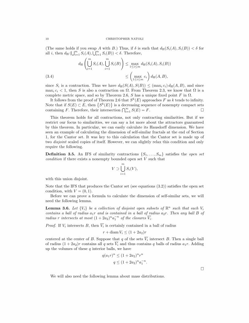
10 CHRISTOPHER NATOLI
(The same holds if you swap A with B.) Thus, if δ is such that dH(Si(A), Si(B)) < δ forall i, then dH (
⋃mi=1 Si(A),
⋃mi=1 Si(B)) < δ. Therefore,
dH
(m⋃i=1
Si(A),
m⋃i=1
Si(B)
)≤ max
1≤i≤mdH(Si(A), Si(B))
≤(
max1≤i≤m
ci
)dH(A,B),(3.4)
since Si is a contraction. Thus we have dH(S(A), S(B)) ≤ (maxi ci) dH(A,B), and sincemaxi ci < 1, then S is also a contraction on Ω. From Theorem 2.3, we know that Ω is acomplete metric space, and so by Theorem 2.6, S has a unique fixed point F in Ω.
It follows from the proof of Theorem 2.6 that Sk(E) approaches F as k tends to infinity.Note that if S(E) ⊂ E, then
Sk(E)
is a decreasing sequence of nonempty compact sets
containing F . Therefore, their intersection⋂∞i=1 S(E) = F .
This theorem holds for all contractions, not only contracting similarities. But if werestrict our focus to similarities, we can say a lot more about the attractors guaranteedby this theorem. In particular, we can easily calculate its Hausdorff dimension. We haveseen an example of calculating the dimension of self-similar fractals at the end of Section1, for the Cantor set. It was key to this calculation that the Cantor set is made up oftwo disjoint scaled copies of itself. However, we can slightly relax this condition and onlyrequire the following.
Definition 3.5. An IFS of similarity contractions S1, . . . , Sm satisfies the open setcondition if there exists a nonempty bounded open set V such that
V ⊃m⋃i=1
Si(V ),
with this union disjoint.
Note that the IFS that produces the Cantor set (see equations (3.2)) satisfies the open setcondition, with V = (0, 1).
Before we can prove a formula to calculate the dimension of self-similar sets, we willneed the following lemma.
Lemma 3.6. Let Vi be a collection of disjoint open subsets of Rn such that each Vicontains a ball of radius a1r and is contained in a ball of radius a2r. Then any ball B ofradius r intersects at most (1 + 2a2)na−n1 of the closures Vi.
Proof. If Vi intersects B, then Vi is certainly contained in a ball of radius
r + diamVi ≤ (1 + 2a2)r
centered at the center of B. Suppose that q of the sets Vi intersect B. Then a single ballof radius (1 + 2a2)r contains all q sets Vi and thus contains q balls of radius a1r. Addingup the volumes of these q interior balls, we have
q(a1r)n ≤ (1 + 2a2)nrn
q ≤ (1 + 2a2)na−n1 .
We will also need the following lemma about mass distributions.

FRACTALS AS FIXED POINTS OF ITERATED FUNCTION SYSTEMS 11
Definition 3.7. A measure µ on a set X is a mass distribution if 0 < µ(X) < ∞. Forany subset A of X, we call µ(A) the mass of A.
Lemma 3.8 (Mass distribution principle). Let µ be a mass distribution on F such thatfor some s, there exists c, δ > 0 such that
(3.9) µ(U) ≤ c(diamU)s
for all sets U with diamU ≤ δ. Then Hs(F ) ≥ µ(F )/c and s ≤ dimH F .
Proof. Let Ui be a cover of F with diamUi ≤ δ. Then, by the properties of measuresand equation (3.9),
µ(F ) ≤ µ
(⋃i
Ui
)≤∑i
µ(Ui) ≤ c∑i
(diamUi)s.
Taking the infimum and letting δ tend to 0, we have Hs(F ) ≥ µ(F )/c. Since µ(F ) > 0, wehave dimH F ≥ s.
We can now prove a formula to calculate the dimension of self-similar sets defined byIFSs. This will be similar to our calculation of the dimension of the Cantor set, in that wemust determine lower and upper bounds for the Hausdorff measure of such a set.
Theorem 3.10. Suppose an IFS of contracting similarities S1, . . . , Sm satisfies the openset condition, and let ci be the ratio of each similarity Si. Let F be the attractor of thisIFS. Then dimH F = s, where
(3.11)
m∑i=1
csi = 1.
Also, we have 0 < Hs(F ) <∞.
Proof. Define s according to equation (3.11). Let Ik be the set of all sequences (i1, . . . , ik)where ij ∈ 1, . . . ,m. Also, for any set A and a given sequence (i1, . . . , ik) in Ik, defineAi1,...,ik = Si1 · · · Sik(A). Then since F is a fixed point under the IFS, we have
F =⋃Ik
Fi1,...,ik .
Thus the sets Fi1,...,ik cover F . Note that the mapping Si · · · Sk is a contractingsimilarity with ratio ci1 · · · cik . Therefore,∑
Ik
(diamFi1,...,ik)s =∑Ik
(ci1 · · · cik)s(diamF )s
=(∑
csi1
)· · ·(∑
csik
)(diamF )s
= (diamF )s(3.12)
by equation (3.11). For all δ > 0, we can choose k large enough that (maxi ci)kdiamF ≤ δ.
Since diamFi1,...,ik ≤ (maxi ci)kdiamF , the sets Fi1,...,ik cover F with diamFi1,...,ik ≤ δ
for all sequences (ii, . . . , ik) in Ik. Therefore, Hs(F ) ≤∑Ik(diamFi1,...,ik)s = (diamF )s
by equation (3.12).We will now try to determine a lower bound for Hs(F ). Let I be the set of all infinite
sequences (i1, i2 . . .) with ij ∈ 1, . . . ,m, and let Ii1,...,ik be the subset of I consistingonly of sequences starting with i1, . . . , ik. Then define a mass distribution µ on I letting
12 CHRISTOPHER NATOLI
µ(Iii,...,ik) = (ci1 · · · cik)s. Proving that µ is indeed a measure follows immediately from∑mi=1 µ(Iii,...,ik,i) = µ(Iii,...,ik). It also follows from equation (3.11) that µ(I) = 1, and so
µ is a mass distribution.Define a point xi1,i2,... in F as xi1,i2,... =
⋂∞k=1 Fi1,...,ik . Then for a subset A in F , define
a new mass distribution µ based on µ by letting µ(A) = µ(Ii1,...,ik : xi1,...,ik,... ∈ A).Intuitively, the µ-mass of a set is the µ-mass of the sequences that define the pointsin that set. Note that µ(F ) = µ(I) = 1 since F contains every point xi1,i2,... for each(i1, i2, . . .) in I.
We now want to show that µ satisfies the conditions of Lemma 3.8, which will pro-vide us with the desired lower bound. Let V be the open set guaranteed by the openset condition (see Definition 3.5), i.e., V ⊃
⋃mi=1 Si(V ) with this union disjoint. Letting
S(V ) =⋃mi=1 Si(V ), it follows from Theorem 3.3 that
Sk(V )
converges to F . Therefore,
V i1,...,ik ⊃ Fi1,...,ik for any sequence (i1, . . . , ik).Let B be a ball of radius r < 1 that intersects F . Also, truncate each sequence (i1, i2, . . .)
in I after the first ik at which point
(3.13)
(min
1≤i≤mci
)r ≤ ci1ci2 · · · cik ≤ r,
where c1, . . . , cm are the ratios of the m contracting similarities. Let Q be the finite setof all such truncated sequences. Since V1, . . . , Vm are disjoint, Vi1,...,ik,1, . . . , Vi1,...,ik,m aredisjoint too, and thus all sets Vii,...,ik where (i1, . . . , ik) is a sequence in Q are also disjoint.Furthermore,
(3.14) F =⋃IFi1,i2,... ⊂
⋃QFi1,...,ik ⊂
⋃QV i1,...,ik .
Choose a1 and a2 such that V contains a ball of radius a1 and is contained in a ball ofradius a2. Then for all (i1, . . . , ik) in Q, the set Vi1,...,ik contains a ball of radius ci · · · cka1and is contained in a ball of radius ci · · · cka2. By equation (3.13), every Vi1,...,ik containsa ball of radius (mini cir)a1 and is contained in a ball of radius ra2. Let Q′ be the subsetof Q consisting only of sequences (i1, . . . , ik) such that V i1,...,ik intersects B. By Lemma3.6, there are at most q = (1 + 2a2)n(mini cia1)−n elements in Q′.
Taking the µ-mass of B,
µ(B) = µ(F ∩B)
= µ(Ii1,...,ik : xi1,...,ik,... ∈ F ∩B)
≤ µ
(Ii1,...,ik : xi1,...,ik,... ∈
(⋃QV i1,...,ik
)∩B
)
since F ⊂⋃Q V i1,...,ik by equation (3.14). From the definition of Q′, we have
µ(B) ≤ µ
(Ii1,...,ik : xi1,...,ik,... ∈
⋃Q′V i1,...,ik
)= µ
(⋃Q′Ii1,...,ik
).
Finally, it follows from the properties of the mass distribution µ and equation (3.13) that
µ(B) ≤∑Q′
µ(Ii1,...,ik) =∑Q′
(ci1 · · · cik)s ≤∑Q′
rs = qrs.
FRACTALS AS FIXED POINTS OF ITERATED FUNCTION SYSTEMS 13
It follows that, for any set U contained in a ball BU of radius diamU , we have µ(U) ≤µ(BU ) ≤ q(diamU)s. Then by Lemma 3.8, Hs(F ) ≥ µ(F )/q = 1/q > 0. Thus Hs(F ) is apositive real number and so dimH F = s.
This theorem provides quick ways to calculate dimension of self-similar fractals. Take theCantor set for example. The IFS for which the Cantor set is an attractor is S1(x) = 1
3x
and S2(x) = 1 − 13x; as demonstrated above, this satisfies the open set condition with
V = (0, 1). Thus by Theorem 3.10, the Hausdorff dimension of the Cantor set is s such
that 2(13
)s= 1, or s = log 2
log 3 . Note that this is similar to our previous calculation of the
dimension of the Cantor set in Section 1.
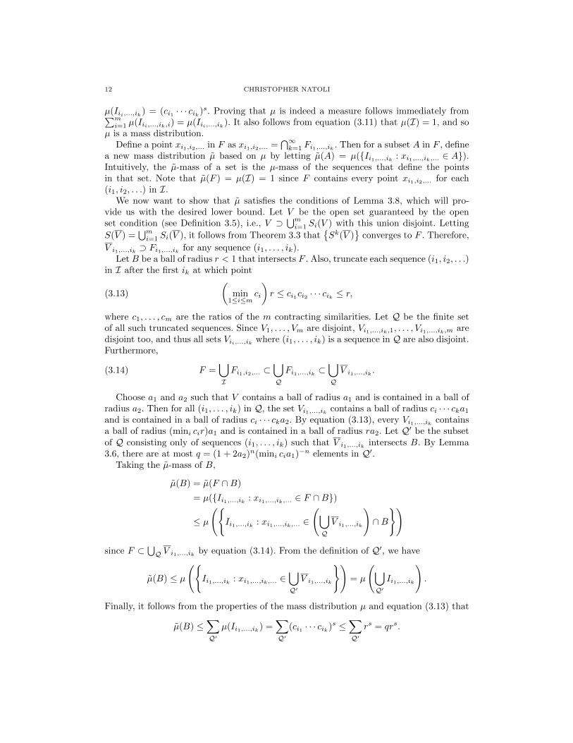
Figure 2. The first itera-tion of the von Koch curve.
We can use this theorem to calculate the dimension ofmany other self-similar fractals. For example, to constructthe von Koch curve, replace the middle third of a straightline segment with the other two sides of an equilateral trian-gle erected on this middle third (see Figure 2). For each iter-ation, repeat this procedure for every segment in the curve.(For the resulting fractal, see Figure 3.) Clearly, the contract-ing similarities are of ratio 1
3 . The open set condition holdswith V as the interior of the tightest isosceles triangle that
contains the von Koch curve, i.e., with the initial segment as the base and a height of√36
times the length of the base. Then the dimension s satisfies 4(13
)s= 1, and so s = log 4
log 3 .
Figure 3. The von Koch curve.
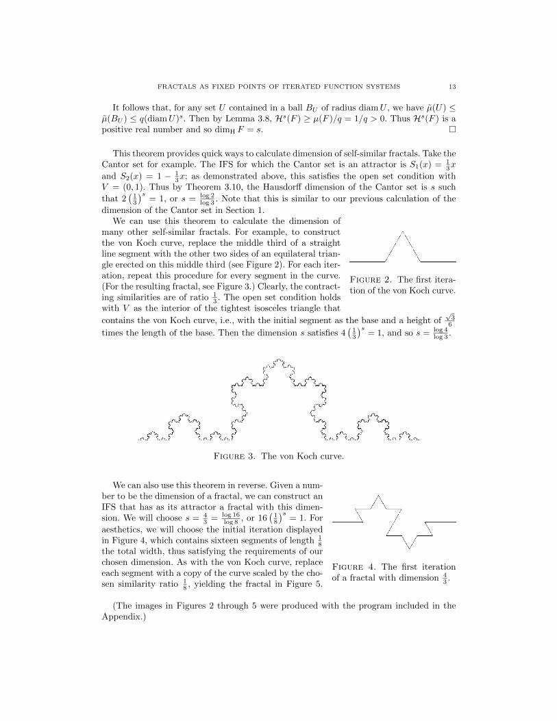
Figure 4. The first iterationof a fractal with dimension 4
3 .
We can also use this theorem in reverse. Given a num-ber to be the dimension of a fractal, we can construct anIFS that has as its attractor a fractal with this dimen-sion. We will choose s = 4
3 = log 16log 8 , or 16
(18
)s= 1. For
aesthetics, we will choose the initial iteration displayedin Figure 4, which contains sixteen segments of length 1
8the total width, thus satisfying the requirements of ourchosen dimension. As with the von Koch curve, replaceeach segment with a copy of the curve scaled by the cho-sen similarity ratio 1
8 , yielding the fractal in Figure 5.
(The images in Figures 2 through 5 were produced with the program included in theAppendix.)

14 CHRISTOPHER NATOLI
Figure 5. A fractal with dimension 43 .
4. Fractals in dynamical systems
Given the iterative nature of fractals, it is not surprising that they show up in dynamicalsystems, in which a function is iterated repeatedly on a set, with each iteration representinganother step in time. To better explore the use of fractals in dynamical systems theory,we must set up the following definitions.
Definition 4.1. Given a continuous mapping f : D → D on a subset D of Rn, let fk
denote the kth iterate of f . Then the system described by the iterations of f on D is adiscrete dynamical system. For a given initial point x in D, the infinite sequence
fk(x)
is
an orbit. If fk(x) settles into an orbit that is a finite set of pointsw, f(w), . . . , fp−1(w)
,
where p is the least positive number such that fp(w) = w, then this set of points is anorbit of period-p points.
It may be the case that fk(x) settles into an orbit of period-1 points, i.e., settles upona fixed point f(w) = w. The iterates fk(x) might also seem to jump about randomly, allthe while approaching a certain set (indeed, often a fractal). To further discuss the sets towhich iterates converge, we will need more terminology.
Definition 4.2. A subset F of D is an attractor for f if F is a closed set such that
• f(F ) = F ;• for all x in an open set V containing F , the distance between fk(x) and F converges
to zero as k tends to infinity; and• for any other set G satisfying the above two conditions, F ⊂ G.
Likewise, F is a repeller if F satisfies the above conditions with the second conditionmodified so that the distance between fk(x) and F diverges as k tends to infinity.
Intuitively, an attractor is a sink. To use a power grid as an example, a house is anattractor, taking energy from a region of the grid surrounding it. This region may besmall, depending on how close other houses are. Extending the analogy, the power stationis a repeller.
A key concern of dynamical systems theory is the behavior of the function f , and inparticular, whether it is chaotic. We will use the following definition.
Definition 4.3. Given a continuous mapping f : D → D on a subset D of Rn, withattractor or repeller F , we say that f exhibits chaotic behavior on F if

FRACTALS AS FIXED POINTS OF ITERATED FUNCTION SYSTEMS 15
• for some x in F , the orbitfk(x)
is dense in F ;
• the periodic points of f in F are dense in F ; and• f has a sensitive dependence on inital conditions, i.e., there exists δ > 0 such that
for all x in F , there exists y in F arbitrarily close to x such that |fk(x)−fk(y)| ≥ δfor some k.
The choice of the word chaotic follows from the fact that f thoroughly “mixes up”points in F , and that a small change in the initial value of x can result in a large changein fk(x). The “butterfly effect”—that a butterfly flapping its wings in Brazil can producea tornado in Texas—follows from this.
With our terminology now established, we will study the Cantor set as an example offractals arising in dynamical systems. In this particular case, the Cantor set is both theattractor of an IFS and the repeller of a dynamical system. Furthermore, the functiondescribing the dynamical system exhibits chaotic behavior in the Cantor set.
The function of interest is
f(x) =3
2(1− |2x− 1|).
If we describe the IFS by the contractions S1, S2 : [0, 1]→ [0, 1], given by S1(x) = 13x and
S2(x) = 1− 13x, we find that f inverts both S1 and S2 on [0, 1], i.e.,
f(S1(x)) = f(S2(x)) = x.
Theorem 3.3 guarantees that there exists a unique attractor C for this IFS, and C =⋂∞k=0 S
k([0, 1]), where S = S1 ∪ S2. Indeed, C is the Cantor set.We will first establish that C is a repeller for f . Since C is an attractor of the IFS, we
have
C = S(C) = S1(C) ∪ S2(C)
f(C) = f(S1(C)) ∪ f(S2(C))
= C ∪ C = C,
and so C satisfies the first condition of being a repeller (see Definition 4.2). Furthermore,note that for x < 0, we have
f(x) =3
2(1 + (2x− 1)) = 3x,
and so fk(x) = 3kx. Therefore, fk(x)→ −∞ as k →∞. For x > 1, we have
f(x) =3
2(1− (2x− 1)) = 3(1− x).
Clearly, f(x) < 0 for all x > 1, and so just one iteration of f brings us to the previouscase, in which x < 0. Thus, again, fk(x) → −∞ as k → ∞. For the final case, namelyx ∈ [0, 1] \ C, there exists some k such that x /∈ Sk([0, 1]), i.e.,
x /∈⋃Si1 Si2 · · · Sik([0, 1]) : ij = 1, 2
f(x) /∈⋃Si2 Si3 · · · Sik([0, 1]) : ij = 1, 2
...
fk(x) /∈ [0, 1].

16 CHRISTOPHER NATOLI
We therefore return to one of the two previous cases, and so fk(x) → −∞. In sum, frepels all x /∈ C to −∞, and the second condition is satisfied.
To prove the final condition, that C is minimal, suppose that C = G1 ∪ G2 with thisunion disjoint and with G1 a repeller under f . Note that for all i, we have Si(G2)∩G1 = ∅,since if Si(G2) and G1 did share some point x, then both f(x) ∈ f(Si(G2)) = G2 andf(x) ∈ f(G1) = G1, which is impossible since G1 and G2 are disjoint. Since S(G2) ⊂ Cbut S(G2) ∩ G1 = ∅, it must be that S(G2) ⊂ G2. But G2 ⊃
⋃∞k=1 S
k(G2 ) = C byTheorem 3.3. Contradiction.
We also wish to prove that f is chaotic in C. Let E in Ω be such that Si(E) ⊂ E fori = 1, 2. Recall that from Theorem 3.3,
C =
∞⋂k=0
Sk(E)
for all such E. Thus, for any x ∈ C, we have x ∈ Si1 · · · Sik(E) for some sequence(i1, . . . , ik) with ij = 1, 2. Extending this sequence gives us a way to express x, namely,
x =
∞⋂k=1
Si1 · · · Sik(E).
We will denote this by x = xi1,i2,.... Observe, first, that this notation is independent of E,and, second, that for any two points xi1,i2,... and xi′1,i′2,... in C such that i1 = i′1, . . . , ik =i′k, we have
|xi1,i2,... − xi′1,i′2,...| ≤ 3−k.
The latter follows from the fact that Si1 is applied last, Si2 is applied second-to-last, andso forth. Also note that xi1,i2,... = S1(xi2,i3,...), and so f(xi1,i2,...) = xi2,i3,...,
For `j = 1, 2, let (`1, `2, . . .) be a sequence containing every n-term sequence of 1sand 2s for all n, e.g., (1, 2, 1, 1, 1, 2, 2, 1, 2, 2, 1, 1, 1, 1, 1, 2, . . .). Thenfor any point xi1,i2,... in C and for all positive integers q, there exists a k such thati1 = `k+1, . . . , iq = `k+q. Therefore,
|xi1,i2,... − x`k+1,`k+2,...| ≤ 3−q
|xi1,i2,... − fk(x`1,`2,...)| ≤ 3−q.
That is to say, for any point xi1,i2,... in C, the iterates fk(x`1,`2,...) are arbitrarily close toxi1,i2,... if q and k are sufficiently large. Therefore, fk(x`1,`2,...) make up dense orbits in C,satisfying the first condition of chaotic behavior.
In addition, the periodic points x`1,...,`p,`1,...,`p,`1,... are dense in C, since for any xi1,i2,...in C, one can construct a periodic point x`1,`2,...,`k,...,`p,`1,... such that i1 = `1, . . . , ik = `k,and therefore
|xi1,i2,... − x`1,`2,...| ≤ 3−k.
Periodic points can thus be made arbitrarily close to any other point in C, and thus theperiodic points are, too, dense in C.
The final condition, that f has a sensitive dependence on initial conditions, is easy toshow. Consider two points xi1,i2,... and xi′1,i′2,... arbitrarily close to each other, as providedby i1 = i′1, . . . , ik = i′k. Let ik+1 = 1 and i′k+1 = 2. Then
fk(xi1,i2,...) = x1,ik+2,... ∈[0, 13]
and fk(xi′1,i′2,...) = x2,i′k+2,...∈[23 , 1].

FRACTALS AS FIXED POINTS OF ITERATED FUNCTION SYSTEMS 17
That is to say, there exists a δ = 13 > 0 such that, given a point xi1,i2,..., there exists an
arbitrarily close point xi′1,i′2,... in C such that
|fk(xi1,i2,...)− fk(xi′1,i′2,...)| = |x1,ik+2,... − x2,i′k+2,...| ≥ δ.
This satisfies the third condition of chaotic behavior.
Acknowledgments. It is a pleasure to thank my mentor, Max Engelstein, for his guid-ance and feedback during the research and writing that led to this paper. His enthusiasmfor the material, challenging expectations, and constant patience and support were in-strumental to writing this paper and making it an instructive and enjoyable experience. Iwould also like to thank Professor Peter May for his generous support in organizing theUniversity of Chicago REU, which has made this all possible.
References
[1] Kenneth Falconer. Fractal Geometry: Mathematical Foundations and Applications. John Wiley & Sons,
2003.[2] Frank Morgan. Geometry Measure Theory. Academic Press, 2009.
[3] Walter Rudin. Principles of Mathematical Analysis. McGraw-Hill, 1964.
[4] William P. Ziemer. Modern Real Analysis. http://www.scribd.com/doc/16597427/24/Hausdor%EF%AC%80-Measure[5] Kenneth Falconer. The Geometry of Fractal Sets. Cambridge University Press, 1985.
[6] Shipan Lu. The Hausdorff Dimension and Measure of Some Cantor Sets. Real Analysis Exchange,Volume 25, Number 2 (1999).
[7] Jeff Henrikson. Completeness and Total Boundedness of the Hausdorff Metric. MIT Undergraduate
Journal of Mathematics. www-math.mit.edu/phase2/UJM/vol1/HAUSF.PDF[8] Michael Slone, Chi Woo. Hausdorff metric inherits completeness. PlanetMath.org.
http://planetmath.org/HausdorffMetricInheritsCompleteness.html.
[9] Margherita Barile and Eric W. Weisstein. Cantor Set. MathWorld–A Wolfram Web Resource.http://mathworld.wolfram.com/CantorSet.html
Appendix
The images in Figures 2 through 5 were produced with the following Python program.
# This program was designed and written by Christopher Natoli.
# It makes use of the Pyglet library to handle graphics and user interface.
# It can be run with Python 2.7.
import math
import pyglet
from pyglet.gl import *
################################################################################
# helper functions
def tuple_scale(tup, ratio):
return tuple([elem*ratio for elem in tup])
def increment_pair(pair, val0, val1):
return (pair[0]+val0, pair[1]+val1)
def increment_list(li, val0, val1):

18 CHRISTOPHER NATOLI
return [increment_pair(pair, val0, val1) for pair in li]
################################################################################
# geometric functions
def find_angle(a,b):
if a[0]==b[0] and a[1]==b[1]: # same point
return -100
return math.atan2(b[1]-a[1], b[0]-a[0])
def rotate_pt(pt, theta): # uses a rotation matrix
return ( pt[0]*math.cos(theta)-pt[1]*math.sin(theta),
pt[0]*math.sin(theta)+pt[1]*math.cos(theta) )
################################################################################
# fractal class ("Frack") and some examples
class Frack:
def __init__(self, vertices, segments):
self.vertices = vertices
self.segments = segments
def scale(self, ratio):
return Frack([tuple_scale(point, ratio) for point in self.vertices],
self.segments)
def rotate(self, theta):
return Frack([rotate_pt(point, theta) for point in self.vertices],
self.segments)
quad_koch = Frack( [ (0.0, 0.25), (0.25, 0.25), (0.25, 0.0),
(0.5, 0.0), (0.5, 0.25), (0.5, 0.5),
(0.75, 0.5), (0.75, 0.25), (1.0, 0.25) ],
[ (0,1), (1,2), (2,3), (3,4), (4,5), (5,6), (6,7), (7,8) ]
)
treelike = Frack( [ (0.0, 0.333), (0.333, 0.333), (0.333, 0.666),
(0.666, 0.333), (0.666, 0.0), (1.0, 0.333) ],
[ (0,1), (1,2), (1,3), (3,4), (3,5) ]
)
koch = Frack( [ (0.0, 0.0),(0.333, 0.0),(0.5, 0.2887),(0.666, 0.0),(1.0,0.0) ],
[ (0,1), (1,2), (2,3), (3,4) ]
)
square_koch = Frack( [ (0.0, 0.0), (0.333, 0.0), (0.333, 0.25),
(0.666, 0.25), (0.666, 0.0), (1.0, 0.0) ],
[ (0,1), (1,2), (2,3), (3,4), (4,5) ]
)

FRACTALS AS FIXED POINTS OF ITERATED FUNCTION SYSTEMS 19
seong = Frack( [ (0.0, 0.2165), (0.125, 0.2165), (0.25, 0.2165),
(0.1875, 0.32476), (0.3125, 0.32476), (0.375, 0.433),
(0.4375, 0.32476), (0.5625, 0.32476), (0.5, 0.2165),
(0.4375, 0.10825), (0.5625, 0.10825), (0.625, 0.0),
(0.6875, 0.10825), (0.8125, 0.10825), (0.75, 0.2165),
(0.875, 0.2165), (1.0, 0.2165)
],
[ (0,1), (1,2), (2,3), (3,4), (4,5), (5,6), (6,7), (7,8),
(8,9), (9,10), (10,11), (11,12), (12,13), (13,14), (14,15),
(15,16) ]
)
################################################################################
# fractal functions
def center_generator(gen):
#lower all points in generator by y-value of first pt
return Frack(increment_list(gen.vertices, 0, -gen.vertices[0][1]),
gen.segments)
def iterate(generator, iteration):
new_vertices = []
new_segments = []
for seg in iteration.segments:
a = iteration.vertices[seg[0]]
b = iteration.vertices[seg[1]]
theta = find_angle(a,b)
if theta==-100:
print("Error in finding angle.")
return
leng = math.sqrt((a[0]-b[0])**2 + (a[1]-b[1])**2)
copy = center_generator(generator.scale(leng)).rotate(theta)
new_segments.extend(increment_list(copy.segments,
len(new_vertices),
len(new_vertices)))
new_vertices.extend(increment_list(copy.vertices, a[0], a[1]))
return Frack(new_vertices, new_segments)
################################################################################
# drawing and graphics functions
width = 900
height = 700
window = pyglet.window.Window(width,height)
glClearColor(1,1,1,1) # white background

20 CHRISTOPHER NATOLI
def draw_line(a,b):
glColor4f(0,0,0,1.0)
glBegin(GL_LINES)
glVertex2f(a[0],a[1])
glVertex2f(b[0],b[1])
glEnd()
def max_height(frack):
max_so_far = 0
for point in frack.vertices:
if point[1] > max_so_far:
max_so_far = point[1]
return max_so_far
def center_frack(frack):
y_offset = (height/2) - (max_height(frack)/2)
return Frack(increment_list(frack.vertices,0,y_offset),frack.segments)
def draw_frack(frack): # draws single iteration only
for seg in frack.segments:
draw_line(frack.vertices[seg[0]],frack.vertices[seg[1]])
def draw_fractal(gen):
current_iter = center_frack(gen.scale(width))
for i in range(4): # user can choose number of iterations here
glClear(GL_COLOR_BUFFER_BIT)
current_iter = iterate(gen, current_iter)
draw_frack(current_iter)
@window.event
def on_draw():
glClear(GL_COLOR_BUFFER_BIT)
############################
# user can choose which fractal to draw by uncommenting only
# the desired fractal
#draw_fractal(quad_koch)
#draw_fractal(treelike)
#draw_fractal(koch)
#draw_fractal(square_koch)
draw_fractal(seong)
############################
pyglet.image.get_buffer_manager().get_color_buffer().save(’screenshot.png’)
# the image will be saved as a file called ’screenshot.png’

FRACTALS AS FIXED POINTS OF ITERATED FUNCTION SYSTEMS 21
pyglet.app.run()
This program produces fractals from user-specified generators (i.e., the first iterationsof fractals). To produce the next iteration, it scales and then copies the generator ontoeach segment of the previous iteration. The contractions of the IFS are determined by thelengths of the segments of the generator.
This program is designed to be flexible so that users may create their own fractals. Todo so, users must specify the details of the generator, namely, the locations of the verticesand which vertices are connected by segments. This is done by writing an instance of theFrack class. The variables quad_koch, treelike, koch, square_koch, and seong are allexamples of generators (koch produced the fractal in Figure 3 and seong produced thefractal in Figure 5). The total width of the generator must be 1. There are no restrictionson the height, although it is expected that the fractal will be wider than it is high (this canbe changed, however, by changing the dimensions of the image as defined by the width
and height variables). The lowest point on the generator must have a y-coordinate of 0.0.The segments list in the Frack class determines which points of the vertices list areconnected. Note that this program was written with fractals only produced from segmentsin mind. Also note that the program may take some time to draw the iterations. One canreduce this time by reducing the number of iterations drawn (it is currently set at 4).
![Modelling Vegetation Through Fractal Geometrymorrow/336_14/papers/irina.pdf · A proof can be found in Michael Barnsley’s Fractals Everywhere. [1, pg 38] 3 Iterated Function Systems](https://static.fdocuments.in/doc/165x107/5f12f0359e1be306d254cb06/modelling-vegetation-through-fractal-geometry-morrow33614papersirinapdf-a.jpg)