FPGA TECHNOLOGY MAPPING FOR FRACTURABLE LOOK-UP …
160
FPGA TECHNOLOGY MAPPING FOR FRACTURABLE LOOK-UP TABLE MINIMIZATION by David Robert Dickin B.A.Sc., Simon Fraser University, 2008 T HESIS SUBMITTED IN PARTIAL FULFILLMENT OF THE REQUIREMENTS FOR THE DEGREE OF MASTER OF A PPLIED S CIENCE IN THE S CHOOL OF E NGINEERING S CIENCE c David Robert Dickin 2011 SIMON FRASER UNIVERSITY Summer 2011 All rights reserved. However, in accordance with the Copyright Act of Canada, this work may be reproduced, without authorization, under the conditions for Fair Dealing. Therefore, limited reproduction of this work for the purposes of private study, research, criticism, review, and news reporting is likely to be in accordance with the law, particularly if cited appropriately.
Transcript of FPGA TECHNOLOGY MAPPING FOR FRACTURABLE LOOK-UP …

FPGA TECHNOLOGY MAPPING FOR
FRACTURABLE LOOK-UP TABLE MINIMIZATION
by
David Robert Dickin
B.A.Sc., Simon Fraser University, 2008
THESIS SUBMITTED IN PARTIAL FULFILLMENT
OF THE REQUIREMENTS FOR THE DEGREE OF
MASTER OF APPLIED SCIENCE
IN THE
SCHOOL
OF
ENGINEERING SCIENCE
c© David Robert Dickin 2011SIMON FRASER UNIVERSITY
Summer 2011
All rights reserved. However, in accordance with the Copyright Act of Canada,this work may be reproduced, without authorization, under the conditions forFair Dealing. Therefore, limited reproduction of this work for the purposes ofprivate study, research, criticism, review, and news reporting is likely to be
in accordance with the law, particularly if cited appropriately.

APPROVAL
Name: David Robert Dickin
Degree: Master of Applied Science
Title of Thesis: FPGA Technology Mapping for Fracturable Look-Up TableMinimization
Examining Committee: Dr. Ash Parameswaran, P.Eng.Professor of Engineering ScienceChair
Dr. Lesley Shannon, P.Eng.Assistant Professor of Engineering ScienceSenior Supervisor
Dr. Marek SyrzyckiProfessor of Engineering ScienceSupervisor
Dr. Glenn Chapman, P.Eng.Professor of Engineering ScienceInternal Examiner
Date Defended:
ii
lib m-scan11
Typewritten Text
11 August 2011

Last revision: Spring 09
Declaration of Partial Copyright Licence The author, whose copyright is declared on the title page of this work, has granted to Simon Fraser University the right to lend this thesis, project or extended essay to users of the Simon Fraser University Library, and to make partial or single copies only for such users or in response to a request from the library of any other university, or other educational institution, on its own behalf or for one of its users.
The author has further granted permission to Simon Fraser University to keep or make a digital copy for use in its circulating collection (currently available to the public at the “Institutional Repository” link of the SFU Library website <www.lib.sfu.ca> at: <http://ir.lib.sfu.ca/handle/1892/112>) and, without changing the content, to translate the thesis/project or extended essays, if technically possible, to any medium or format for the purpose of preservation of the digital work.
The author has further agreed that permission for multiple copying of this work for scholarly purposes may be granted by either the author or the Dean of Graduate Studies.
It is understood that copying or publication of this work for financial gain shall not be allowed without the author’s written permission.
Permission for public performance, or limited permission for private scholarly use, of any multimedia materials forming part of this work, may have been granted by the author. This information may be found on the separately catalogued multimedia material and in the signed Partial Copyright Licence.
While licensing SFU to permit the above uses, the author retains copyright in the thesis, project or extended essays, including the right to change the work for subsequent purposes, including editing and publishing the work in whole or in part, and licensing other parties, as the author may desire.
The original Partial Copyright Licence attesting to these terms, and signed by this author, may be found in the original bound copy of this work, retained in the Simon Fraser University Archive.
Simon Fraser University Library Burnaby, BC, Canada

Abstract
Modern commercial Field-Programmable Gate Array (FPGA) architectures contain look-
up tables (LUTs) that can be “fractured” into two smaller LUTs. The potential to pack
two LUTs into a space that could accommodate only one LUT in traditional architectures
complicates FPGA technology mapping’s resource minimization objective. Previous works
introduced edge recovery techniques and the concept of LUT balancing, both of which
produce mappings that pack into fewer fracturable LUTs. We combine these two ideas and
evaluate their effectiveness for one commercial and four academic FPGA architectures, all
of which contain fracturable LUTs. When combined, edge-recovery and LUT balancing
yield a 9.0% to 16.1% reduction in fracturable LUT use, depending on the architecture.
We also present a modified technology mapping algorithm called MO-Map that reduces
fracturable LUT utilization by 9.7% to 17.2%.
iii

Acknowledgments
Thank you to my wonderful wife Diana. It is because of your unending love and support
that I was able to finish my degree. To my parents, brother, and sister: thank you for believ-
ing that I would finish... eventually. Thanks to the many friends I have made throughout
my graduate studies at Simon Fraser University for making the graduate school experience
a friendly and fun one. Lastly, a big thank you to my supervisor, Dr. Lesley Shannon. You
have been a wonderful person to work with and I am interminably indebted to you for the
guidance and support you have given me.
I would also like to acknowledge the financial support and equipment that I have re-
ceived from the following organizations that made my research possible: the Canadian
Microelectronics Corporation, the Natural Sciences and Engineering Research Council,
Xilinx, Altera, and Simon Fraser University.
iv

Contents
Approval ii
Abstract iii
Acknowledgments iv
Contents v
List of Tables ix
List of Figures xii
Glossary xv
1 Introduction 1
1.1 Motivation . . . . . . . . . . . . . . . . . . . . . . . . . . . . . . . . . . . 2
1.2 Objective . . . . . . . . . . . . . . . . . . . . . . . . . . . . . . . . . . . 3
1.3 Contributions . . . . . . . . . . . . . . . . . . . . . . . . . . . . . . . . . 4
1.4 Thesis Organization . . . . . . . . . . . . . . . . . . . . . . . . . . . . . . 5
2 Background 6
v

CONTENTS vi
2.1 Field-Programmable Gate Array Architecture . . . . . . . . . . . . . . . . 6
2.1.1 Fracturable LUTs . . . . . . . . . . . . . . . . . . . . . . . . . . . 10
2.2 FPGA CAD Tool Flow . . . . . . . . . . . . . . . . . . . . . . . . . . . . 12
2.3 FPGA Technology Mapping . . . . . . . . . . . . . . . . . . . . . . . . . 14
2.3.1 Overview . . . . . . . . . . . . . . . . . . . . . . . . . . . . . . . 15
2.3.2 FPGA Technology Mapping Objectives . . . . . . . . . . . . . . . 17
2.3.3 General FPGA Technology Mapping Algorithm . . . . . . . . . . . 18
2.3.4 Cut Enumeration . . . . . . . . . . . . . . . . . . . . . . . . . . . 18
2.3.5 Mapping for Minimum Depth . . . . . . . . . . . . . . . . . . . . 20
2.3.6 Mapping for Minimum Area . . . . . . . . . . . . . . . . . . . . . 20
2.3.7 Deriving the Final Mapping . . . . . . . . . . . . . . . . . . . . . 22
2.4 Complete Cut Enumeration Alternatives . . . . . . . . . . . . . . . . . . . 23
2.5 Technology Mapping for Fracturable LUTs . . . . . . . . . . . . . . . . . 26
3 Technology Mapping for FLUT Minimization 28
3.1 The Minimum Number of Fractruable LUTs . . . . . . . . . . . . . . . . . 28
3.2 Technology Mapping Techniques for Minimal
Fracturable LUTs . . . . . . . . . . . . . . . . . . . . . . . . . . . . . . . 31
3.3 MO-Map: Multiple-Output Map . . . . . . . . . . . . . . . . . . . . . . . 33
4 Experimental Methodology 37
4.1 Synthesis and Technology Mapping . . . . . . . . . . . . . . . . . . . . . 37
4.2 Packing, Placement, and Routing Experimental Setup . . . . . . . . . . . . 40
4.2.1 Academic Tool Flow . . . . . . . . . . . . . . . . . . . . . . . . . 40
4.2.2 Commercial Tool Flow . . . . . . . . . . . . . . . . . . . . . . . . 44

CONTENTS vii
5 Experimental Results 46
5.1 Experimental Results without LUT balancing . . . . . . . . . . . . . . . . 46
5.1.1 Technology Mapping without LUT balancing . . . . . . . . . . . . 47
5.1.2 Packing without LUT balancing . . . . . . . . . . . . . . . . . . . 50
5.2 LUT Balancing Experiments . . . . . . . . . . . . . . . . . . . . . . . . . 58
5.2.1 Technology Mapping Results . . . . . . . . . . . . . . . . . . . . 58
5.2.2 Packing Results . . . . . . . . . . . . . . . . . . . . . . . . . . . . 67
5.3 Placement and Routing Results . . . . . . . . . . . . . . . . . . . . . . . . 75
5.3.1 Maximum Operating Frequency . . . . . . . . . . . . . . . . . . . 75
5.3.2 Minimum Channel Width and Wirelength . . . . . . . . . . . . . . 77
5.4 Estimating the Impact on Silicon Area . . . . . . . . . . . . . . . . . . . . 85
6 Conclusions and Future Work 87
6.1 Conclusions . . . . . . . . . . . . . . . . . . . . . . . . . . . . . . . . . . 87
6.1.1 Future Work . . . . . . . . . . . . . . . . . . . . . . . . . . . . . 90
Bibliography 92
Appendix A FLUT utilizations - no LUT balancing 99
Appendix B LUT distribution data 107
Appendix C FLUT utilization - with LUT balancing 112
Appendix D VPR Minimum Channel Width Geometric Means 123
Appendix E VPR Wirelength Geometric Means 132

CONTENTS viii
Appendix F Quartus II Fmax Geometric Means 141

List of Tables
4.1 Benchmark suite circuits with baseline mapping statistics. . . . . . . . . . . 41
5.1 Runtime and LUT count of the mapped benchmark circuits. . . . . . . . . . 48
5.2 FLUT utilization for each tech-mapper/architecture combination. . . . . . . 56
5.3 LUT balancing Weight(6) and Weight(5) values that minimized average
FLUT utilization for each tech-mapper/architecture combination. . . . . . . 74
5.4 Increase in minimum channel width for the benchmark suite packings that
have the greatest average FLUT minimization. . . . . . . . . . . . . . . . . 84
5.5 Estimate of percent change in silicon area. . . . . . . . . . . . . . . . . . . 86
A.1 Benchmark circuit’s FLUT utilization when mapped without LUT balanc-
ing and packed for the M5 FPGA architecture. . . . . . . . . . . . . . . . . 99
A.2 Benchmark circuit’s FLUT utilization when mapped without LUT balanc-
ing and packed for the M6 FPGA architecture. . . . . . . . . . . . . . . . . 101
A.3 Benchmark circuit’s FLUT utilization when mapped without LUT balanc-
ing and packed for the M7 FPGA architecture. . . . . . . . . . . . . . . . . 102
A.4 Benchmark circuit’s FLUT utilization when mapped without LUT balanc-
ing and packed for the M8 FPGA architecture. . . . . . . . . . . . . . . . . 103
ix

LIST OF TABLES x
A.5 Benchmark circuit’s FLUT utilization when mapped without LUT balanc-
ing and packed for the Stratix II FPGA architecture. . . . . . . . . . . . . . 105
B.1 ClassicMap LUT distribution data . . . . . . . . . . . . . . . . . . . . . . 107
B.2 WireMap LUT distribution data . . . . . . . . . . . . . . . . . . . . . . . 109
B.3 MO-Map LUT distribution data . . . . . . . . . . . . . . . . . . . . . . . 110
C.1 Benchmark suite’s FLUT utilization geometric mean for mappings pro-
duced with LUT balancing and packed for the M5 FPGA architecture. . . . 113
C.2 Benchmark suite’s FLUT utilization geometric mean for mappings pro-
duced with LUT balancing and packed for the M6 FPGA architecture. . . . 115
C.3 Benchmark suite’s FLUT utilization geometric mean for mappings pro-
duced with LUT balancing and packed for the M7 FPGA architecture. . . . 117
C.4 Benchmark suite’s FLUT utilization geometric mean for mappings pro-
duced with LUT balancing and packed for the M8 FPGA architecture. . . . 119
C.5 Benchmark suite’s FLUT utilization geometric mean for mappings pro-
duced with LUT balancing and packed for the Stratix II FPGA architecture. 121
D.1 Benchmark suite’s minimum channel width (MCW) geometric mean for
mappings produced with LUT balancing and packed for the M5 FPGA ar-
chitecture. . . . . . . . . . . . . . . . . . . . . . . . . . . . . . . . . . . . 124
D.2 Benchmark suite’s minimum channel width (MCW) geometric mean for
mappings produced with LUT balancing and packed for the M6 FPGA
architecture. . . . . . . . . . . . . . . . . . . . . . . . . . . . . . . . . . . 126

LIST OF TABLES xi
D.3 Benchmark suite’s minimum channel width (MCW) geometric mean for
mappings produced with LUT balancing and packed for the M7 FPGA
architecture. . . . . . . . . . . . . . . . . . . . . . . . . . . . . . . . . . . 128
D.4 Benchmark suite’s minimum channel width (MCW) geometric mean for
mappings produced with LUT balancing and packed for the M8 FPGA ar-
chitecture. . . . . . . . . . . . . . . . . . . . . . . . . . . . . . . . . . . . 130
E.1 Benchmark suite’s wirelength geometric mean for mappings produced with
LUT balancing and packed for the M5 FPGA architecture. . . . . . . . . . 133
E.2 Benchmark suite’s wirelength geometric mean for mappings produced with
LUT balancing and packed for the M6 FPGA architecture. . . . . . . . . . 135
E.3 Benchmark suite’s wirelength geometric mean for mappings produced with
LUT balancing and packed for the M7 FPGA architecture. . . . . . . . . . 137
E.4 Benchmark suite’s wirelength geometric mean for mappings produced with
LUT balancing and packed for the M8 FPGA architecture. . . . . . . . . . 139
F.1 Benchmark suite’s maximum operating frequency geometric mean for
mappings produced with LUT balancing and packed for the Stratix
II FPGA architecture. . . . . . . . . . . . . . . . . . . . . . . . . . . . . . 142

List of Figures
2.1 An example block diagram of an island-style FPGA. . . . . . . . . . . . . 7
2.2 A Basic Logic Element (BLE), which contains a single LUT and flip-flop
pair. . . . . . . . . . . . . . . . . . . . . . . . . . . . . . . . . . . . . . . 8
2.3 A Complex Logic Block (CLB) that contains a cluster of BLEs. . . . . . . 9
2.4 An SRAM-based LUT with a K of 3. . . . . . . . . . . . . . . . . . . . . . 10
2.5 Xilinx Virtex-5 fracturable LUT block diagram. . . . . . . . . . . . . . . . 11
2.6 FLUT models for fractured mode and regular mode operation. . . . . . . . 12
2.7 FPGA CAD Tool Flow. . . . . . . . . . . . . . . . . . . . . . . . . . . . . 13
2.8 An example Boolean logic function to be technology mapped for an FPGA. 16
2.9 Top level pseudo-code describing a general cut-based FPGA technology
mapping algorithm. . . . . . . . . . . . . . . . . . . . . . . . . . . . . . . 19
2.10 Exact Area computation pseudo-code. . . . . . . . . . . . . . . . . . . . . 22
2.11 Final mapping derivation pseudo-code. . . . . . . . . . . . . . . . . . . . . 23
2.12 Top level pseudo-code for the priority cuts technology mapping algorithm. . 25
3.1 Potential LUT pairings to be implemented in a fractured mode FLUT with
a K of 6 and a M of 5. . . . . . . . . . . . . . . . . . . . . . . . . . . . . . 30
xii

LIST OF FIGURES xiii
3.2 Top level pseudo-code for the priority cuts technology mapping algorithm
with MO-Map. . . . . . . . . . . . . . . . . . . . . . . . . . . . . . . . . 34
3.3 Pseudo-code for the MO-Map area recovery function. . . . . . . . . . . . . 36
4.1 A generic version of the CLB used in the four academic FPGA architec-
tures targeted by VPR with AAPack. . . . . . . . . . . . . . . . . . . . . . 42
5.1 LUT distributions for ClassicMap, WireMap, and MO-Map without LUT
balancing. . . . . . . . . . . . . . . . . . . . . . . . . . . . . . . . . . . . 49
5.2 Percent reduction in FLUT usage relative to the baseline for each circuit
in the benchmark suite. Packed for the M5 FPGA architecture using VPR
with AAPack. . . . . . . . . . . . . . . . . . . . . . . . . . . . . . . . . . 51
5.3 Percent reduction in FLUT usage relative to the baseline for each circuit
in the benchmark suite. Packed for the M6 FPGA architecture using VPR
with AAPack. . . . . . . . . . . . . . . . . . . . . . . . . . . . . . . . . . 52
5.4 Percent reduction in FLUT usage relative to the baseline for each circuit
in the benchmark suite. Packed for the M7 FPGA architecture using VPR
with AAPack. . . . . . . . . . . . . . . . . . . . . . . . . . . . . . . . . . 53
5.5 Percent reduction in FLUT usage relative to the baseline for each circuit
in the benchmark suite. Packed for the M8 FPGA architecture using VPR
with AAPack. . . . . . . . . . . . . . . . . . . . . . . . . . . . . . . . . . 54
5.6 Percent reduction in ALM usage relative to the baseline for each circuit
in the benchmark suite. Packed for the Stratix II FPGA architecture using
Quartus II. . . . . . . . . . . . . . . . . . . . . . . . . . . . . . . . . . . . 55
5.7 LUT distributions for ClassicMap with different Weight(6) values. . . . . . 59

LIST OF FIGURES xiv
5.8 LUT distributions for WireMap with different Weight(6) values. . . . . . . 60
5.9 LUT distributions for MO-Map with different Weight(6) values. . . . . . . 61
5.10 LUT distributions for ClassicMap with varying Weight(5) and Weight(6). . . 64
5.11 LUT distributions for WireMap with varying Weight(5) and Weight(6). . . . 65
5.12 LUT distributions for MO-Map with varying Weight(5) and Weight(6). . . . 66
5.13 Academic architectures FLUT resource utilization for mappings with vary-
ing Weight(6). . . . . . . . . . . . . . . . . . . . . . . . . . . . . . . . . . 68
5.14 Stratix II ALM resource utilization for mappings with varying Weight(6). . 69
5.15 Academic architectures FLUT resource utilization for mappings with vary-
ing Weight(5) and Weight(6). . . . . . . . . . . . . . . . . . . . . . . . . . 71
5.16 Stratix II ALM resource utilization for mappings with varying Weight(5)
and Weight(6). . . . . . . . . . . . . . . . . . . . . . . . . . . . . . . . . . 72
5.17 Average maximum operating frequency reported by Quartus II. . . . . . . . 76
5.18 Academic architecture minimum channel widths for mappings with vary-
ing Weight(6). . . . . . . . . . . . . . . . . . . . . . . . . . . . . . . . . . 79
5.19 Academic architecture minimum channel widths for mappings with vary-
ing Weight(5) and Weight(6). . . . . . . . . . . . . . . . . . . . . . . . . . 80
5.20 Academic architecture wirelengths for mappings with varying Weight(6). . 81
5.21 Academic architecture wirelengths for mappings with varying Weight(5)
and Weight(6). . . . . . . . . . . . . . . . . . . . . . . . . . . . . . . . . . 82

Glossary
AAPack Architecture Aware Packer
AF Area Flow
ALM Adaptive Logic Module
ASIC Application Specific Integrated Circuit
BLE Basic Logic Element
BLIF Berkeley Logic Interchange Format
CAD Computer Aided Design
CLB Complex Logic Block
Fmax Maximum Operating Frequency
FPGA Field-Programmable Gate Array
HDL Hardware Description Language
I/O Input and Output
IC Integrated Circuit
LAB Logic Array Block
MCNC Microelectronics Center North Carolina
MCW Minimum Channel Width
xv

GLOSSARY xvi
MO-Map Multiple-Output Map
QUIP Quartus II University Interface Program
SRAM Static Random Access Memory
VPR Versatile Place and Route
VQM Verilog Quartus Mapping
Chapter 1
Introduction
Field-Programmable Gate Arrays (FPGAs) are reconfigurable integrated circuits that have
traditionally implemented Boolean logic using look-up tables (LUTs). A LUT can imple-
ment any function with up to K inputs (a K-LUT), where K is an architectural parameter.
Technology mapping (tech-mapping) is the process of converting a technology-independent
netlist into a netlist composed solely of primitive elements available for implementation on
a target device. The resulting netlist is referred to as a mapping. Performing tech-mapping
for a FPGA primarily entails mapping logic into LUTs (mapping for other FPGA elements,
such as memories, multipliers, etc, also occurs).
One goal of FPGA tech-mapping is to minimize the number of LUTs in the mapping,
i.e. the area of the mapping. Modern commercial FPGA architectures use Fracturable
LUTs (FLUTs) instead of basic LUTs. A FLUT can operate as either a single normal LUT,
or as two smaller LUTs with input-sharing constraints. This “fracturability” feature ensures
that the number of FLUTs utilized will always be less than or equal to the number of LUTs
in the mapping. Thus, the number of LUTs is not an accurate metric for evaluating the area
of a mapping for FPGA architectures with FLUTs. Technology mapping techniques that
1

CHAPTER 1. INTRODUCTION 2
minimize the number of FLUTs, not LUTs, are desirable for modern FPGA architectures.
1.1 Motivation
Modern commercial FPGAs from Xilinx [1] and Altera [2] feature FLUTs instead of the
traditional LUT. A FLUT is a structure that can operate as either a single K-LUT, or be
“fractured” into two (K-1)-LUTs with input-sharing constraints. The two (K-1)-LUTs only
have access to a fixed number of unique inputs, M, which necessitates the two (K-1)-LUTs
either have inputs in common or unused input pins. The LUTs in a mapping are packed into
FLUTs, either individually or in pairs, during later stages of the FPGA Computer Aided
Design (CAD) tool flow.
The fact that two LUTs can potentially pack into a single FLUT ensures that the number
of FLUTs utilized on an FPGA is always less than or equal to the number of LUTs in the
mapping. Thus, the number of LUTs in the mapping is no longer a definitive measure
of how many logic resources a design will occupy on an FPGA. Although the number of
LUTs in a mapping is still important, the number of inputs each LUT in a mapping uses
is also consequential. LUTs that use the majority of their K inputs will be harder to pack
together into the two “fractured” (K-1)-LUTs of a FLUT. When technology mapping for
a FLUT-based FPGA architecture, the area metric “number of LUTs” is flawed. It is the
mapping that packs into smallest number of FLUTs that uses the least number of logic
resources. Therefore, technology mapping algorithms that produce mappings that pack
into fewer FLUTs are desirable.

CHAPTER 1. INTRODUCTION 3
1.2 Objective
Two previous works have been shown to produce mappings that pack into fewer FLUTs.
Modifying the cost functions in the technology mapping algorithm to discourage the se-
lection of LUTs that use all K of their inputs is called LUT balancing [3]. LUT balancing
was found to provide benefit when mapping for Altera Stratix II FPGAs [4]. Another op-
tion is the WireMap technology mapper [5][6]. WireMap used edge-recovery heuristics to
minimize the number of wires in a mapping and was shown to reduce FLUT utilization for
Xilinx Virtex-5 FPGAs by virtue of generating mappings with reduced routing demands.
Using LUT balancing or WireMap during technology mapping causes the final map-
ping to contain more LUTs than usual. However, the LUTs in the mapping tend to pack
into FLUTs more efficiently, resulting in lower logic resource usage if the target FPGA ar-
chitecture has FLUTs. Although both techniques have the same advantage (a more “pack-
able” mapping) and disadvantage (a greater number of LUTs in the mapping), they are
implemented using different mechanisms in the technology mapping algorithm. The mech-
anisms are compatible, raising the question of whether or not LUT balancing and WireMap
are complementary and can be used in combination to further reduce the FLUT count.
In the previous works, the effectiveness of WireMap was demonstrated using the Xilinx
Virtex-5 while LUT balancing’s effects were shown using the Altera Stratix II. One of the
many differences between these two architectures is the number of unique inputs available
to their FLUTs (The M parameter). Therefore, we are also interested in how the value of
M affects the packability of our mappings.
The objective of this research is to identify technology mapping methods that minimize
FLUT usage after packing. We adopt a three-pronged approach to achieving this goal:
• Study whether the edge-recovery techniques of WireMap can be combined with the

CHAPTER 1. INTRODUCTION 4
concept of LUT Balancing to enhance FLUT minimization.
• Evaluate the effects of different FLUT input-sharing constraints (i.e. M value) on a
mapping’s packability.
• Investigate improvements to technology mapping algorithms for FLUT minimiza-
tion.
1.3 Contributions
This thesis can be divided into three main contributions:
• Combining WireMap with our LUT balancing schemes and analyzing the results to
find the best parameters for FLUT minimization.
• Quantification of the interaction between the M parameter and a mappings packabil-
ity.
• An enhancement to the tech-mapping algorithm, called Multiple-Output Map (MO-
Map), that is combined with WireMap and LUT balancing to further reduce FLUT
usage.
We explore the relative improvements gained by combining WireMap and our imple-
mentation of LUT balancing. The quality of a mapping is evaluated using the reduction in
FLUT usage after packing the mapping. The mappings are packed for four FLUT-based
FPGA architectures with different M values using a new version of the Versatile Place and
Route (VPR) software that includes the Architecture Aware Packer (AAPack) [7][8]. Two

CHAPTER 1. INTRODUCTION 5
of these academic architectures emulate the FLUTs found in commercial FPGAs. In addi-
tion, we use Quartus University Interface Program (QUIP) [9] to run the mappings through
Altera’s Quartus II software targeting a Stratix II [4] FPGA. When WireMap and LUT
balancing are used, the average percent reduction in FLUT utilization, relative to map-
pings produced without WireMap or LUT balancing, ranged from 6.9% to 16.1% across
the architectures. When MO-Map is used, the average percent reduction in FLUT usage is
between 9.0% and 17.2% for the various architectures.
1.4 Thesis Organization
The remainder of the thesis is structured as follows. Chapter 2 provides background on
FPGA architecture and the CAD tool flow, particularly tech-mapping. Chapter 3 describes
our LUT Balancing implementation and MO-Map. Chapter 4 explains our experimental
methodology. Chapter 5 presents the experimental results. Chapter 6 concludes the thesis
and outlines future work.

Chapter 2
Background
This chapter presents background material related to the contributions of this thesis. We
begin by giving an overview of FPGA architecture and the FPGA CAD tool flow. We then
outline common terminology and concepts used in FPGA technology mapping algorithms.
Finally, prior work on FPGA technology mapping is discussed.
2.1 Field-Programmable Gate Array Architecture
FPGAs are integrated circuits that are manufactured to be reconfigurable. Reconfigurability
is achieved by using static random access memory (SRAM) elements to specify the logic
functions implemented by LUTs and routing connectivity. A SRAM-based FPGA can be
configured to implement some desired circuit functionality, and reconfigured repeatedly as
required by the designer. This reconfigurability is a notable advantage of a FPGA when
compared to an Application Specific Integrated Circuit (ASIC). A design implemented on
an ASIC should be able to operate faster, use less power, and occupy a smaller area than
a FPGA implementation [10]. Although, the ASIC will be significantly more expensive to
6

CHAPTER 2. BACKGROUND 7
I/O I/O I/O I/O I/O I/O I/O
I/O I/O I/O I/O I/O I/O I/OI/O
I/O
I/O
I/O
I/O
I/O
I/O
I/O
I/O
I/O
I/O
I/O
I/O
I/O
I/OI/O
I/OI/O
Complex
Logic
Block
Complex
Logic
Block
Complex
Logic
Block
Complex
Logic
Block
Complex
Logic
Block
Complex
Logic
Block
Complex
Logic
Block
Complex
Logic
Block
Complex
Logic
Block
Figure 2.1: An example block diagram of an island-style FPGA.
create and have a slower time to market.
This thesis focuses on the class of FPGA architectures known as island-style FPGAs,
an example of which is depicted in Figure 2.1. An island-style FPGA consists of a grid of
Complex Logic Blocks (CLBs) set in an interconnect framework. The CLBs contain LUTs
and flip-flops to perform computation tasks while the interconnect framework consists of
many programmable wires used to connect the CLBs together. Around the periphery of the
CLB grid are Input/Output (I/O) blocks.

CHAPTER 2. BACKGROUND 8
BLE
4-LUT
D flip-flop
D Q
In1
In4
clk
In2
In3
Out
Figure 2.2: A Basic Logic Element (BLE), which contains a single LUT and flip-flop pair.
An island-style FPGA that has identical CLBs throughout is a homogeneous FPGA
architecture. It is common in modern FPGA architectures to include specialized circuitry,
referred to as hard blocks, in addition to the general purpose CLBs. Some examples of
specialized circuits commonly found in commercial FPGAs are memories, multipliers, and
multi-gigabit transceivers. An FPGA architecture that includes these additional circuits is
a heterogeneous architecture.
Figure 2.2 shows a Basic Logic Element (BLE), which contains a single LUT and flip-
flop pair along with a 2-1 multiplexor that determines whether the registered or unregistered
LUT output drives the output. A LUT can implement an arbitrary Boolean logic function
with up to K inputs, where K is an architectural parameter (K is four in Figure 2.2). Flip-
flops provide the memory elements required for implementing sequential circuits. It is
common for the CLBs of academic FPGA architectures to contain some number of BLEs.
Figure 2.3 illustrates a CLB that contains a cluster of BLEs. CLBs contain LUTs and
flip-flops, usually in the form of BLEs, along with the routing elements required to connect
to the FPGA’s interconnect framework. A CLB may also contain other special purpose
circuitry, such as carry-chain logic. The organization of LUTs and flip-flops within a CLB
varies greatly between different FPGA architectures. A common arrangement is for the

CHAPTER 2. BACKGROUND 9
Local
Interconnect 4-LUT D flip-flop
D Q
4-LUT D flip-flop
D Q
4-LUT D flip-flop
D Q
CLB
Figure 2.3: A Complex Logic Block (CLB) that contains a cluster of BLEs.
CLB to contain a cluster of BLEs along with fast local interconnect connecting the BLEs
in the cluster [11].
One example of a how a LUT is constructed is shown in Figure 2.4. Here we have an
SRAM-based LUT with K equal to 3. The “SRAM Configuration Memory” is a bank of
2K SRAM bits that is programmed with the desired Boolean logic function’s truth table
when the FPGA is configured. The K select lines of the multiplexor tree are the LUT’s
inputs and choose which configuration SRAM bit value is propagated to the LUT’s output.
The FPGA’s interconnect framework is comprised of wire segments and switches. The
switches are programmable and control which wire segments are connected together as well

CHAPTER 2. BACKGROUND 10
bit0
bit1
bit2
bit3
bit4
bit5
bit6
bit7
In1 In2 In3
OutS
RA
M C
on
fig
ura
tio
n M
em
ory
Figure 2.4: An SRAM-based LUT with a K of 3.
as which wire segments connect to CLBs. The wire segments vary in length and run in both
horizontal and vertical directions. Depending on the architecture, the wire segments may
be uni-directional or bi-directional links. Modern FPGAs use uni-directional links because
they have been found to be faster while occupying a similar area footprint [12].
2.1.1 Fracturable LUTs
As of 2011, modern commercial FPGAs, such as the Xilinx Virtex-5 and the Altera Stratix
II, have fracturable look-up tables (FLUTs). A FLUT is a LUT with the ability to be
fractured, which means it can function as either a single large LUT (regular mode) or two
smaller LUTs (fractured mode). A FLUT can be constructed using two LUTs and a 2-to-1
multiplexor. As an example, Figure 2.5 shows a block diagram of the FLUT found in the
Xilinx Virtex-5 FPGA [13][14][15].
The Virtex-5 FLUT is a “dual-output 6-LUT”. The FLUT has six inputs, two outputs,
and encapsulates two 5-LUTs as well as a 2-to-1 multiplexor. When the FLUT is operated

CHAPTER 2. BACKGROUND 11
Virtex-5 FLUT
5-LUT
5-LUT
In1In2In3In4In5In6
Out1
Out2
Figure 2.5: Xilinx Virtex-5 fracturable LUT block diagram.
in regular mode it functions as a standard 6-LUT (K is six for the Virtex-5). To operate as a
6-LUT, one 5-LUT implements the logic function assuming In1 is high and the other 5-LUT
implements the function assuming In1 is low. The In1 signal selects which 5-LUT drives
Out1, the output of the 6-LUT, and the Out2 signal is unused. If the FLUT is operated in
fractured mode, the In1 signal is programmed to always select the output of the top 5-LUT
as the driver of Out1 and the bottom 5-LUT drives Out2. Thus, in fractured mode each
FLUT output is driven by one of the 5-LUTs.
Since the Virtex-5 FLUT only has six inputs, and one of those inputs is dedicated to the
multiplexor, the two 5-LUTs may only have five unique inputs between them. Clearly, this
imposes a constraint upon which LUTs can be packed into a FLUT operating in fractured
mode. Like the Virtex-5, the Altera Stratix II FLUT [16][3][4] has a K equal to six, meaning
it operates as a 6-LUT in regular mode. However, the Stratix II FLUT has eight unique
inputs that can be used by the two fractured mode 5-LUTs, instead of only five.
In this thesis, we use the parameter M to specify the number of unique inputs a FLUT

CHAPTER 2. BACKGROUND 12
(K-1)
Regular ModeFractured Mode
(K-1)-Input
LUT
(K-1)-Input
LUT
(K-1)
M
KK-Input
LUT
Figure 2.6: FLUT models for fractured mode and regular mode operation.
has when operating in fractured mode (M is five for the Virtex-5 FLUT and eight for the
Stratix II.). We also assume that the two fractured mode LUTs have K minus one inputs.
Figure 2.6 depicts the generic models we use for FLUTs operating in fractured and regular
mode.
2.2 FPGA CAD Tool Flow
Circuits are typically specified in a Hardware Description Language (HDL) such as Verilog
or VHDL. To convert an HDL circuit description into a configuration bitstream for an
FPGA, the HDL is passed through a CAD tool flow. The steps that compose a typical
FPGA CAD tool flow are shown in Figure 2.7. The academic software programs (i.e.
programs for which the source code is available) - ODIN II [17], ABC [18], T-VPack [19],
AAPack [7][8], and VPR [20] - that can perform each of these operations are included in
brackets beneath each step in the figure.
The first step of the FPGA CAD flow is HDL elaboration, where the HDL is converted
into a technology-independent netlist. Next technology independent synthesis is performed
to optimize the netlist. Once optimizations are complete, technology mapping is performed,

CHAPTER 2. BACKGROUND 13
HDL Design
Technology Independent Synthesis
(Odin II, ABC)
Technology Mapping
(ABC)
Clustering (i.e. Packing)
(T-Vpack, AAPack)
Placement
(VPR)
Routing
(VPR)
FPGA Configuration
HDL Elaboration
(Odin II)
Figure 2.7: FPGA CAD Tool Flow.
which maps the technology-independent netlist into a netlist of primitives available on the
FPGA (i.e. LUTs, flip-flops, hard blocks, etc). This netlist of primitives is called a mapped
netlist, or mapping. This thesis is primarily concerned with the technology mapping stage
of the CAD flow.
After technology mapping is the packing or clustering stage. During packing, the prim-
itives in the mapping (LUTs and flip-flops) are grouped into CLBs. If the FPGA archi-
tecture has FLUTs, then part of the packing process involves packing LUTs into FLUTs.
After packing is placement, where the elements of the packed netlist (CLBs, hard blocks,

CHAPTER 2. BACKGROUND 14
I/Os) are assigned to specific locations on the FPGA. Finally, routing occurs to determine
a configuration of the FPGA’s interconnect framework that will to connect all the elements
of the system together.
Packing is the stage of the CAD flow when LUTs are packed into FLUTs and is of par-
ticular interest to our work because FLUT utilization numbers are available after packing.
The older academic clustering tool T-VPack is not capable of packing LUTs into FLUTs
and is therefore not used in our experiments. However, the recently introduced AAPack
tool is capable. AAPack has been incorporated into VPR as part of the Verilog-to-Routing
project [21], and is the only academic FPGA CAD software we are aware of that supports
FPGA architectures with FLUTs during packing.
In addition to the academic software tools mentioned previously, Altera and Xilinx pro-
vide a CAD tool suite for use with their products. It is possible to integrate portions of the
academic tool flow with Altera’s Quartus II software suite using the functionality provided
by QUIP [9]. Methods also exist for interacting with the Xilinx CAD tools [22][23][24].
2.3 FPGA Technology Mapping
For LUT-based FPGAs, the technology mapping problem is to cover a Boolean network us-
ing K-LUTs to obtain a functionally equivalent K-LUT network. The conventional library-
based method of technology mapping used for ASICs is inappropriate for LUT-based FP-
GAs due to the large number of functions a LUT can implement. In this section, we define
terminology related to FPGA technology mapping, outline FPGA tech-mapping objectives,
and provide a description of a general FPGA technology mapping algorithm based on pre-
vious works in the field.

CHAPTER 2. BACKGROUND 15
2.3.1 Overview
A Boolean network can be represented as a Directed Acyclic Graph (DAG). The vertices
(nodes) of the DAG represent logic gates and the directed edges correspond to wires con-
necting the gates. The DAG also has primary inputs (PIs) and primary outputs (POs) rep-
resenting the pins of the circuit. If the circuit is sequential, it will include registers. Each
register is treated as an additional PI and PO in the DAG. The DAG is called the subject
graph, and is the input to a technology mapping tool (tech-mapper).
The AND-Inverter Graph (AIG) format is a useful way of presenting a subject graph
for synthesis and technology mapping [25]. Boolean logic in an AIG is implemented us-
ing only Inverters and 2-input AND gates. As an example, consider the Boolean logic in
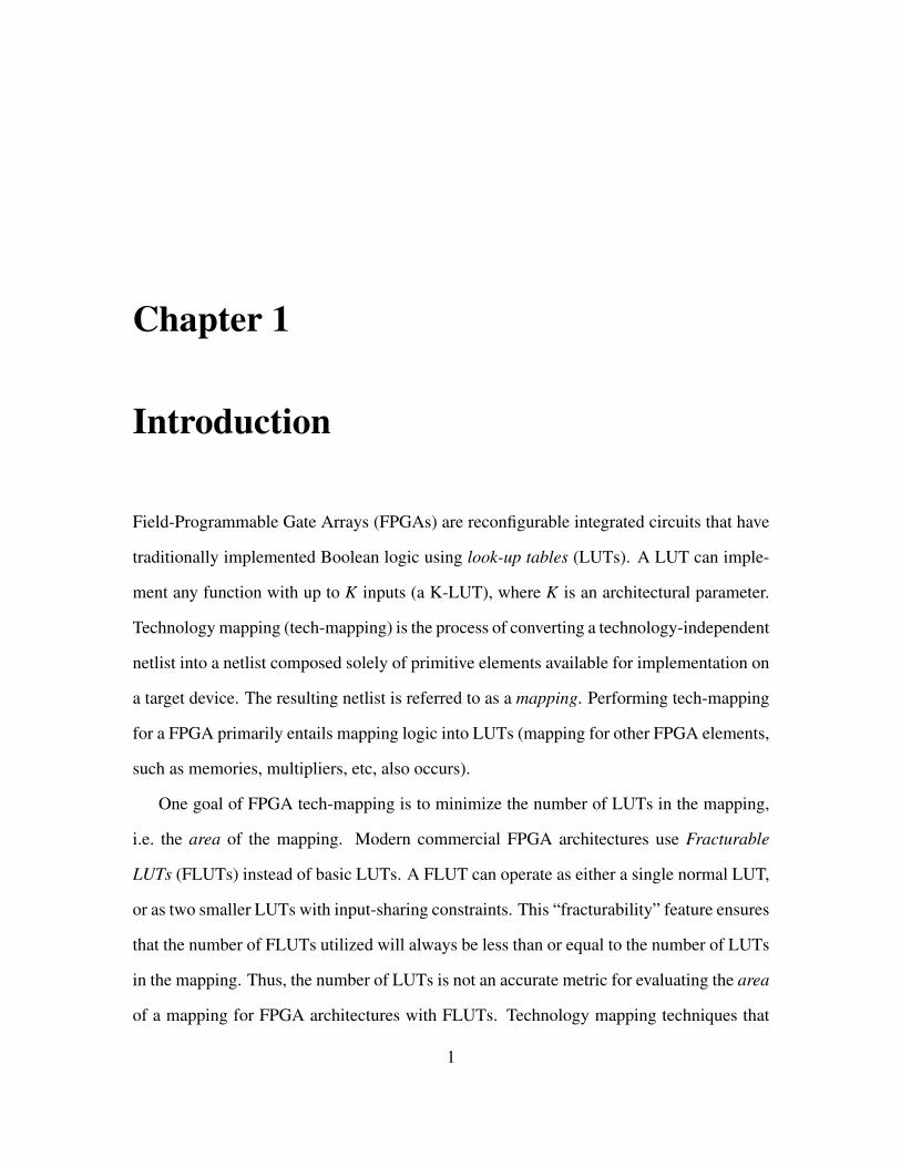
Equation 2.1. Figure 2.8(a) illustrates the Boolean network for the equation, Figure 2.8(b)
shows the network converted to an AIG, and Figure 2.8(c) is the DAG representation.
Z = A + B + (C ·D) (2.1)
FPGA technology mapping commonly employs the notion of cuts. A cut is a set of leaf
nodes (leaves) in the subject graph associated with a particular root node. A set of leaf
nodes constitutes a cut of a root node if all paths from the PIs to the root node pass through
one or more leaf nodes. A cut is said to cover the root node and every node on the paths
between the leaves and the root, but not the leaves themselves. Figure 2.8(d) identifies the
three cuts of the DAG node n3 from Figure 2.8(b). Each quadrangle with a dotted line
corresponds to a cut. All nodes covered by the cut are contained within the quadrangle.
Each node that has a directed edge going into the quadrangle is a leaf of the cut. The node
n3 is the root node of the three cuts. The three cuts are {A, B, n2}, {C, D, n1}, and {n1,
CHAPTER 2. BACKGROUND 16
A B C D
Z
(a) The Boolean network.
A B C D
Z
(b) The Boolean network as an AIG.
A B C D
Z
n1 n2
n3
(c) The AIG as a DAG.
A B C D
Z
n1 n2
n3
(d) The three cuts of node n3.
Figure 2.8: An example Boolean logic function to be technology mapped for an FPGA.

CHAPTER 2. BACKGROUND 17
n2}.
If a cut has K or less leaf nodes, the cut is K-feasible. A K-feasible cut can be im-
plemented using a K-LUT. A tech-mapper computes K-feasible cuts for all nodes in the
subject graph, then selects a number of these cuts to form a mapped circuit (i.e. mapping)
of the subject graph. A mapping is a network of K-feasible cuts (i.e. LUTs) that covers all
of the nodes in the subject graph.
2.3.2 FPGA Technology Mapping Objectives
The primary optimization goal of LUT-based FPGA technology mapping is typically to
minimize the mapped circuit’s delay. The unit delay model, which assumes that each LUT
on a path imposes a unit of delay, is common during technology mapping because no
routing details are known at this early stage of the CAD tool flow. Under the unit-delay
model, a mapping’s delay is equal to its depth. The depth of a mapping is determined by
the path from a PI to a PO that has the largest number of LUTs on it. The number of
LUTs on that path is the depth. Thus, technology mapping for depth minimization under
the unit-delay model is equivalent to mapping for minimum delay. FlowMap was the first
algorithm to optimally solve the LUT-based FPGA technology mapping problem for depth
minimization in polynomial time based using network flow computation [26].
Another common objective is to minimize the area of the mapped network. The area of
a mapping is measured as the number of LUTs included in the mapping. LUT minimization
has been shown to be a non-deterministic polynomial-time hard (NP-hard) problem [27].
This reason LUT count is used as an area metric, as opposed to silicon area, is that the
FPGA is already fabricated and the size of each LUT is constant. The LUT count deter-
mines how many logic resources on the FPGA must be used to implement the mapping.

CHAPTER 2. BACKGROUND 18
Technology mapping algorithms often combine these two objectives and map for min-
imum area under delay constraints. With this approach, the first priority is finding the
minimum mapping depth (delay), and then minimizing the mapping’s area while maintain-
ing this depth. A downside to this approach is area duplication, where more LUTs are
used than strictly necessary in order to minimize the depth of the circuit at the cost of addi-
tional area. Algorithms that can perform these tasks include CutMap [28], DAOmap [29],
IMap [30], and the LUT-based FPGA technology mapping tools included in ABC [31][32].
Other technology mapping algorithms, such as PowerMap [33], PowerMinMap [34],
Emap [35] and DVmap [36], aim to minimize power, which is also an NP-hard prob-
lem [37]. Routability is another objective tackled by RMap [38] and WireMap [5][6].
2.3.3 General FPGA Technology Mapping Algorithm
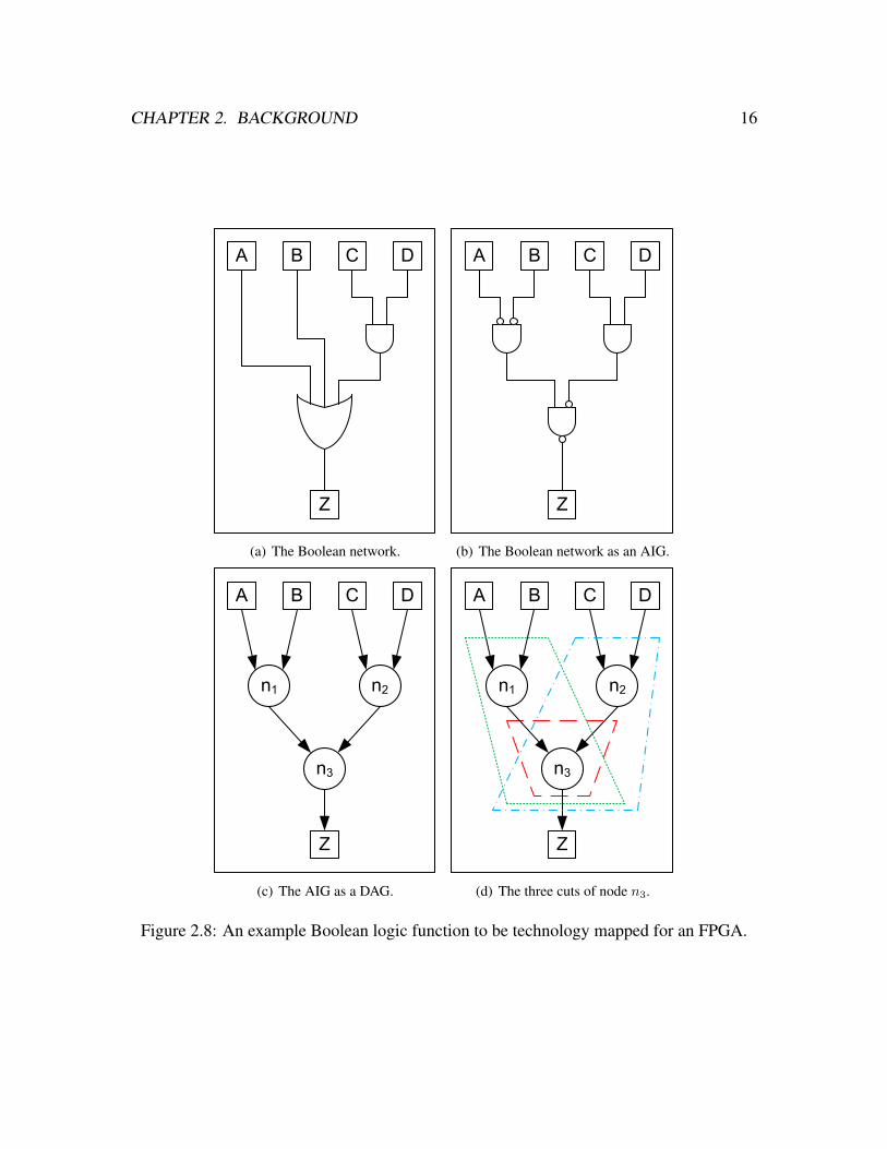
This section reviews a general cut-based FPGA technology mapping algorithm based on
previous works [26][29][31]. The top level pseudo-code for the algorithm is provided in
Figure 2.9. The algorithm operates on a subject graph in AIG form, aig, and maps to LUTs
with at most K inputs. The objective of the algorithm is to first minimize the depth of a
circuit, and then map for minimal area (i.e. LUT count) while maintaining the depth.
2.3.4 Cut Enumeration
The cut-set of a node, n, is the set of all enumerated K-feasible cuts that have n as the root
node. The EnumerateCuts function of Figure 2.9 visits each node in the AIG in topolog-
ical order and computes the cut-set of the node as per the methods presented in previous
works [39][40][32]. The cut-set of a node is computed by considering all combinations of
the node’s fanins cut-sets along with the trivial cut of the node. The fanins of a node, n, are
CHAPTER 2. BACKGROUND 19
TechnologyMap( aig, K )
{
// compute K-feasible cuts for each node
EnumerateCuts( aig, K );
// select min-depth cut as the representative cut for each node
MapMinDepth( aig, K );
// select min-area cut as representative for non-critical nodes
MapAreaRecover( aig, K );
// determine set of cuts that will be LUTs in the mapping
DeriveFinalMapping( aig, K );
}
Figure 2.9: Top level pseudo-code describing a general cut-based FPGA technology map-ping algorithm.
the nodes in the graph that have a directed edge pointing to n (the fanouts are the nodes n
has directed edges pointing to). The trivial cut of a node, n, is composed solely of the node
itself.
To explain the cut computation procedure, let A and B be two cut-sets and ♦ be the
operator for creating a new set of K-feasible cuts from two cut-sets. The operation A♦B is
defined as:
A♦B = {u ∪ v|u ∈ A, v ∈ B, |u ∪ v| ≤ K} (2.2)
Now let the cut-set of a node, n, be denoted by Φ(n) and let n1 and n2 be the fanins of
n. Φ(n) is computed using Equation 2.3.
Φ(n) =
{{n}} if n ∈ PI
{{n}} ∪ Φ(n1)♦Φ(n2) otherwise
(2.3)
Traversing the graph in topological order ensures that the cut-sets of the fanins, Φ(n1)

CHAPTER 2. BACKGROUND 20
and Φ(n2), have been computed prior to the cut computations for n.
2.3.5 Mapping for Minimum Depth
Once all the cuts have been computed and stored by the EnumerateCuts function of Fig-
ure 2.9, the MapMinDepth function is run to find the minimum depth of the mapping.
Again the AIG graph is traversed in a topological order, at each node the cuts of the cut-set
are compared against each other and the one with the minimum depth is selected as the
representative cut of the node. The representative cut of a node is the “best” cut according
to some optimization objective, in this case depth. Frequently, multiple cuts in the cut-set
will have equivalent depth. In this case, additional cost functions are computed in order to
break the tie and select a representative cut.
The depth of a cut under the unit delay model is equal to one plus the largest depth of
its leaf’s representative cuts. A PI node’s depth is zero as its cut-set consists only of the
trivial cut, and thus has no leaves. The PO node with the largest depth determines the depth
of the mapping, which is what we are trying to minimize when performing depth optimal
technology mapping. If all possible cuts are enumerated for all nodes in the graph and the
representative cut of each node is the cut in the cut-set with the smallest depth, then the
mapping’s depth is guaranteed to be optimal [26].
2.3.6 Mapping for Minimum Area
The MapAreaRecover function of Figure 2.9 is run once the minimum depth of the circuit
has been determined. This is done to change the representative cuts of nodes with non-
critical depth requirements to minimize the number of LUTs in the mapping. Unlike depth,
the optimal area of the mapping is not determined due to the NP-hard nature of the problem.

CHAPTER 2. BACKGROUND 21
Instead, heuristics are used to try and minimize area in a reasonable amount of time.
As in the MapMinDepth function, the graph is traversed in a topological order and the
cuts in each cut-set are compared. This time a cost function that measures area is used
instead of depth as the basis for comparison when determining the new representative cut.
To ensure that the circuit depth does not degrade, the new representative cut’s depth cannot
exceed the node’s maximum depth value, which was determined during the MapMinDepth
function call. Multiple passes of the graph may be performed with different area cost
functions.
The two cost functions used in ABC for evaluating the area of cuts are Area Flow and
Exact Area [31][32]. Both functions include a Weight() function, which returns the base
cost of a cut depending upon how many leaves the cut has. By default, Weight() returns 1.0
irregardless of the number of leaves.
The Area Flow (AF) [30] (effective area [39]) of a cut is used to give a global view of
the area of a cut. The Area Flow of a cut, c is computed using Equation 2.4,
AF (c) = Weight(nLeaves(c)) +∑
i
AF (BestCut(Leafi(c)))
nEstFanouts(Leafi(c))(2.4)
where BestCut(Leafi(c)) is the representative cut of the i-th leaf of c and
nEstFanouts(Leafi(c)) is the estimated number of fanouts the i-th leaf of c will have in
the mapping. If nEstFanouts(Leafi(c)) is zero, then the denominator in Equation 2.4 is set
to one to avoid division by zero.
The Exact Area of a cut provides a local view of the area of a cut. Exact Area is
calculated by summing the Weight() of all cuts added to the mapping as a result of including
c. This computation is recursive and requires keeping a reference counter for each node
that counts how many times the node is used in the current mapping. Pseudo-code for the

CHAPTER 2. BACKGROUND 22
float ComputeExactArea( cut c )
{
// set the base area of the cut
float Area = Weight(nLeaves(c));
foreach leaf of c
{
// increment the leaf’s reference counter
RefCnt(leaf)++;
// recurse if the leaf not yet part of the mapping
if ( RefCnt(leaf) == 1 )
Area += ComputeExactArea(BestCut(leaf));
}
// return the exact area of the cut c
return Area;
}
Figure 2.10: Exact Area computation pseudo-code.
Exact Area calculation of a cut, c, is given in Figure 2.10. After the computation, another
recursive function must be called to reset the reference counters to their previous values if
the cut is not included in the mapping.
2.3.7 Deriving the Final Mapping
The final step in our general FPGA technology mapping algorithm is the DeriveFinalMap-
ping function. In this function, a set of representative cuts, which together cover all nodes
in the DAG, is selected. This set of cuts forms the final mapping that is output by the tech-
mapper (recall that a K-feasible cut can be implemented by a LUT). Pseudo code for the
DeriveFinalMapping function is shown in Figure 2.11.
The DeriveFinalMapping function calls the AddToMapping function for each PO. The
AddToMapping function adds the representative cut of the PO to the mapping as a LUT,

CHAPTER 2. BACKGROUND 23
DeriveFinalMapping( aig, K )
{
// loop for all PO’s
foreach PO in aig
AddToMapping(PO);
}
// function to add the representative cut of a node to the mapping
AddToMapping( node n )
{
// cut variable
cut c = BestCut(n);
// check if we should add this node
if ( !( InMapping(n) ) && !( IsPI(n) ) )
{
// add the representative cut of this node to the mapping
AddLutToMapping(c);
// recurse for the leaves
foreach leaf in c
AddToMapping(leaf);
}
}
Figure 2.11: Final mapping derivation pseudo-code.
and then recursively calls itself for all leaves of the representative cut that are not already
part of the mapping or a PI.
2.4 Complete Cut Enumeration Alternatives
For a circuit with m nodes, the number of K-feasible cuts for a node can be as large a
O(mK) [41]. Computing and storing all of the cuts for each node in a circuit can be time
consuming and memory intensive. A number of techniques have been proposed to handle
the large number of cuts that may be enumerated for larger circuits and high K values.
One approach is to perform cut ranking and pruning [39]. In this approach, cuts are

CHAPTER 2. BACKGROUND 24
ranked according to the current cost function and the cuts that rank so poorly that they
are unlikely to generate “good” cuts for other nodes are discarded (i.e. “pruned”). The
maximum number of cuts that each node is allowed to store can also be capped, typically
at some large number (e.g. 2000).
Another approach is the use of factor cuts [31]. The factor cuts of a node are a subset
of the cut-set. Using factor cuts, it is possible to generate the other cuts in the cut-set
when needed. Factor cuts were found to produce better delays and shorter run-times than
conventional cut enumeration when the number of cuts each node is allowed to store is
capped.
The notion of priority cuts [32] can be used to dramatically reduce the runtime and
memory footprint of an FPGA tech-mapper. Priority cuts places a small cap (e.g. 8) on the
number of cuts that can be stored for each node. To compensate for the small number of
cuts generated, additional mapping passes are performed. The additional mapping passes
use a variety of primary cost functions and tie-breaker cost functions when ranking the
generated cuts. The benefit of priority cuts is reduced runtime because fewer cuts are
generated and ranked, and a smaller memory footprint as fewer of the enumerated cuts are
stored. A downside of this approach (and other approaches that do not perform complete
cut enumeration) is that the algorithm cannot guarantee depth optimality. However, in
practice the minimum depth found is often the same as that of a depth-optimal algorithm.
Figure 2.12 gives pseudo code for the priority cuts mapping algorithm. This pseudo
code is a replacement for the general technology mapping pseudo code of Figure 2.9. In
the general algorithm, cuts were enumerated only once using the EnumerateCuts func-
tion and then representative cuts were selected for each node using the MapMinDepth and
MapAreaRecover functions. Unlike the general algorithm, the priority cuts tech-mapper

CHAPTER 2. BACKGROUND 25
PriorityCutsMap( aig, K )
{
// perform multiple mapping passes optimizing for Depth
MappingPassDelay( MinNumInputs );
MappingPassDelay( AreaFlow );
// perform multiple mapping passes optimizing for Area Flow
for ( i = 0 ; i < numAreaFlowPasses ; i++ ) {
MappingPassArea( Area Flow );
}
// perform multiple mapping passes optimizing for Exact Area
for ( i = 0 ; i < numExactAreaPasses ; i++ ) {
MappingPassArea( ExactArea );
}
// determine set of cuts that will be LUTs in the mapping
DeriveFinalMapping( aig, K );
}
Figure 2.12: Top level pseudo-code for the priority cuts technology mapping algorithm.
enumerates cuts during each of its multiple mapping passes. The functions MappingPass-
Delay and MappingPassArea of Figure 2.12 perform a mapping passes that include cut
enumeration and selecting representative cuts. During each pass, cut-sets that are no longer
needed to generate other cut-sets further along in the graph are discarded on the fly to keep
the memory footprint small.
The MappingPassDelay function goes through the AIG graph in topological order and
enumerates and ranks cuts for each node. The highest ranked cuts are those that have the
minimum depth, ties between nodes with equal depth are broken using the criteria spec-
ified in the argument to MappingPassDelay (MinNumInputs or AreaFlow). The highest
ranking cuts are stored as the node’s priority cuts. Once the minimum depth of the graph
has been determined, MappingPassArea calls are made to map the graph while optimiz-
ing for area under depth constraints. Again cuts are enumerated and ranked for nodes in

CHAPTER 2. BACKGROUND 26
a topological order. This time, the ranking algorithm does not consider those cuts whose
depth exceeds the required maximum depth determined for the node during MappingPass-
Delay. The remaining cuts are ranked using the area cost function specified as an argument
to MappingPassArea. After all mapping passes have been completed, the final mapping is
derived in the same manner as the general technology mapping algorithm.
2.5 Technology Mapping for Fracturable LUTs
FPGA technology mapping traditionally produces a netlist of LUTs. These LUTs are later
packed into FLUTs during the packing stage of the CAD tool flow. As a result, the majority
of previous work does not explicitly consider FLUTs during technology mapping. This is
compounded by the fact that until recently, the typical academic CAD tool flow could not
model FPGAs with FLUTs at all. Those works that do take FLUTs into account during
technology mapping are noted in this section.
One previous work presents a method of enumerating KL-cuts [42]. A KL-cut is a
cut with a maximum of K inputs and L outputs. A KL-cut with L equal to two and K
corresponding to the maximum LUT size could potentially map directly to FLUTs instead
of LUTs. They present a covering algorithm that uses KL-cuts, but note that it is not
intended to achieving state-of-the-art in mapping. It would be interesting if their covering
algorithm could be modified to achieve state-of-the-art delay and area characteristics.
Another previous work describes the two-output RAM-based technology mapper called
Hydra [43]. With Hydra, functions that have two outputs are considered early in the map-
ping process instead of during packing. Hydra focuses on area, and thus is not depth-
optimal, and only works for combinatorial circuits.

CHAPTER 2. BACKGROUND 27
The WireMap tech-mapper uses edge-recovery heuristics as part of its cut ranking cost
function [5]. The edge-recovery heuristics were added to the complete cut enumeration
tech-mapper of ABC and the mappings produced were found to occupy 6.3% fewer Virtex-
5 FLUTs after packing [6]. In our work, we use a version of WireMap that has the edge-
recovery techniques incorporated into the priority cuts tech-mapper of ABC. The edge-
recovery heuristics are used as a tie-breaking cost function when ranking cuts. Their use
favours cuts that add fewer edges (wires) to the mapping. A consequence of the edge-
recovery heuristics noted in the previous work is an increase in the number of LUTs that
use only 2, 3, or 4 of their 6 inputs, and a decrease in the number of LUTs that use 5 or 6
of their inputs. It is easier to pack LUTs that use fewer inputs into a fractured mode FLUT.
Recall that FLUTs have a limited number of unique inputs, M, that are available to the two
fractured mode LUTs. LUTs with fewer inputs have a smaller impact on this input-sharing
constraint.
Employing LUT balancing during technology mapping to avoid the inclusion of LUTs
that use all six of their inputs was found to be beneficial when mapping for the Altera Stratix
II, a FPGA whose architecture contains FLUTs [3]. LUT balancing refers to modifying the
cut ranking cost function in order to reduce the number of occurrences of LUTs that use a
certain number of inputs in the mapping. A LUT that uses all six of its inputs (K is six for
the Stratix II) cannot be packed into our FLUT model’s fractured mode, and is therefore
undesirable from a resource usage perspective. Modifying the cut ranking cost functions
to prefer LUTs with a certain number of inputs was previously proposed for heterogeneous
FPGA architectures that had two LUT structures with different numbers of inputs [39].

Chapter 3
Technology Mapping for FLUT
Minimization
A FPGA mapping consists of LUTs, flip-flops, inputs/outputs, various types of hard blocks,
and the connectivity of the elements. The traditional measurement of mapping area is equal
to the number of LUTs in the mapping. When the FPGA has FLUT resources, this measure
of mapping area is inaccurate because two LUTs can potentially be packed into a single
FLUT resource. This chapter outlines the FLUT minimization problem and provides details
about the MO-Map technology mapping algorithm.
3.1 The Minimum Number of Fractruable LUTs
The number of FLUTs that a mapping packs into is given by Equation 3.1.
nFLUT =
⌈nLutTotal + nLutRegMode
2
⌉(3.1)
28

CHAPTER 3. TECHNOLOGY MAPPING FOR FLUT MINIMIZATION 29
The term nLutTotal is the total number of LUTs in the mapping (i.e. the traditional mea-
surement of a mapping’s area). The term nLutRegMode is the number of LUTs that must
be packed into a FLUT operating in regular mode (i.e. not fractured mode). nLutRegMode
is always less than or equal to nLutTotal. Therefore, the number of FLUTs is always less
than or equal to the number of LUTs in the mapping.
The value of nLutTotal is easily obtained during tech-mapping by counting the number
of LUTs in the current mapping. Unfortunately, the total number of LUTs in nLutRegMode
is not available until packing is performed. LUTs that use all K of their inputs must be
packed into a FLUT operating in regular mode (they are too large for fractured mode).
Therefore, LUTs using K inputs are included in the nLutRegMode count and can be counted
during technology mapping. But for LUTs that used K-1 or fewer inputs, it is infeasible
to discern whether or not a LUT should be included in the nLutRegMode count during a
typical FPGA technology mapping process.
In order to pack a LUT with K-1 or fewer inputs into a fractured mode FLUT, a pair
LUT must be identified. The pair LUT is packed into the FLUT along with the original
LUT, and thus must also only use K-1 or fewer inputs. In addition, in order to be packed
together into a FLUT, the two LUTs can only have M unique inputs between them (M is the
number of inputs a FLUT operating in fractured mode has). This input-sharing constraint
means that there is no guarantee that a LUT with K-1 or fewer inputs will be able to find a
suitable pair LUT and could therefore potentially add to the nLutRegMode count.
Figure 3.1 illustrates some potential LUT pairings for a fractured mode FLUT with a
K of 6 and a M of 5. The first pair can be packed together into a fractured mode FLUT
because the LUTs have fewer than K inputs and the total number of unique inputs between
them is less than or equal to M. The second pair of LUTs cannot be packed together into

CHAPTER 3. TECHNOLOGY MAPPING FOR FLUT MINIMIZATION 30
2-LUT
3-LUT
A
B
C
D
E
Each LUT has K-1 or
fewer inputs?
M or less unique
inputs total?
Suitable
Pair
3-LUT
3-LUT
A
B
D
E
F
Each LUT has K-1 or
fewer inputs?
M or less unique
inputs total?
Unsuitable
Pair
C
3-LUT
3-LUT
A
B
C
D
E
Each LUT has K-1 or
fewer inputs?
M or less unique
inputs total?
Suitable
Pair
C
Figure 3.1: Potential LUT pairings to be implemented in a fractured mode FLUT with a Kof 6 and a M of 5.
a FLUT because they have six unique inputs between them, A,B,C,D,E,F, and thus fail to
meet the input-sharing constraint. The last pair of LUTs have a common input, C, reducing
the number of unique inputs to five for the pair, which meets the input-sharing constraint.
Finding suitable pairs of LUTs to pack together into a FLUT is usually performed
during packing, not technology mapping. This is due to the fact that during tech-mapping,
exactly which LUTs are included in the mapping is still being determined. Adding in
the requirement to determine a pair LUT for each cut would increase mapping run-time

CHAPTER 3. TECHNOLOGY MAPPING FOR FLUT MINIMIZATION 31
by orders of magnitude due to the large number of cuts generated by cut enumeration.
There are some previous works that tackle similar problems. KL-cut enumeration identifies
pairs of K-feasible cuts during mapping [42], and a simultaneous mapping and clustering
algorithm has been proposed [44]. But both methods have long run-times, and either don’t
guarantee depth-optimality in the case of the former, or don’t consider FLUTs in the case
of the latter.
The architectural parameter M has a strong influence on how many FLUTs end up
operating in nLutRegMode. The second pair of LUTs in Figure 3.1 cannot fit in a fractured
mode FLUT because they have six unique inputs between them and M is only 5. Had M
been larger, there would be no issue packing the two LUTs together. Of course, a FLUT
with a larger M will occupy more silicon area on the FPGA. Given that the two major FPGA
vendors, Xilinx and Altera, have architectures with different values of M, it is unclear at
this time what values of M are optimal.
3.2 Technology Mapping Techniques for Minimal
Fracturable LUTs
Minimizing Equation 3.1 involves keeping the number of total LUTs small while maximiz-
ing the number of LUTs that can be packed into a fractured mode FLUT. Since the largest
LUTs in the mapping, those with K inputs, are guaranteed to be unable to pack into a frac-
tured mode FLUT, they should be avoided except when necessary to maintain the depth of
a mapping. For LUTs with less than K inputs, it seems intuitive that those with the fewest
inputs will be the easiest to pack into fractured mode FLUTs. This is because they put the
least strain on the input-sharing restriction of a fractured mode FLUT. Unfortunately, LUTs

CHAPTER 3. TECHNOLOGY MAPPING FOR FLUT MINIMIZATION 32
with a small number of inputs tend to cover fewer nodes in the DAG, which requires more
total LUTs be present in the mapping.
In this thesis, we combine two technology mapping techniques from previous works
to technology map with the objective of minimizing FLUT utilization without degrading
mapping depth. The first technique is the edge-recovery heuristics of the WireMap technol-
ogy mapper [5][6]. And the second is the concept of LUT balancing [3]. Both techniques
were introduced in Section 2.5, and both were found to produce mappings that packed into
fewer FLUTs on commercial FPGA architectures.
We use a version of ABC that has the WireMap edge-recovery heuristics incorporated
as an option in the priority cuts tech-mapper in our experiments. This version of ABC is
not a release version, and was provided by Alan Mishchenko, an author of the WireMap
papers [5][6]. The previous works presenting WireMap have the edge-recovery techniques
incorporated into their traditional mapper, not the priority cuts mapper.
The exact modifications to the cut ranking cost functions used to implement LUT bal-
ancing in previous work were not disclosed as the software is proprietary. To implement
LUT-Balancing for our experiments, we modified the value returned by the Weight() func-
tion for cuts with large numbers of inputs. The Weight() function is part of the Area Flow
and Exact Area cost functions from Section 2.3.6, which are used to evaluate the area cost
of cuts in ABC’s tech-mappers. This modification was accomplished using the LUT library
function of ABC, which allows the user to specify the area (i.e. Weight()) and delay (always
set to unit delay) of a cut depending on how many inputs the cut has.
It is our goal to technology map such that FLUT resource usage is minimized without
negatively affecting the mapping’s depth (i.e. map for minimum area under depth con-
straints). To ensure that depth is not compromised during the initial mapping passes of

CHAPTER 3. TECHNOLOGY MAPPING FOR FLUT MINIMIZATION 33
the priority cuts mapper, a Weight() of 1.0 is used for all cuts during the initial mapping
passes. The area cost functions that use Weight() are used to break ties between cuts during
the initial depth-determining mapping passes. Thus, modifying Weight() has an effect upon
which cuts are selected as priority cuts for each node. In early experiments, we observed
the depth of one particular benchmark increased by one if we did not take these precau-
tions. No other modifications to ABC were necessary to implement our version of LUT
balancing.
3.3 MO-Map: Multiple-Output Map
In addition to combining the previous works, WireMap and LUT-Balancing, we sought to
find new tech-mapping techniques for minimizing FLUT usage under delay constraints.
The most successful of our exploratory techniques is presented here under the name
Multiple-Output Map (MO-Map). MO-Map performs an extra area recovery step after
each mapping pass in the ABC priority cuts mapper. Top level pseudo code for the pri-
ority cuts mapping algorithm with MO-Map is shown in Figure 3.2. The additions due to
MO-Map are in bold.
After each mapping pass, the function MoMapAreaRecovery is called to expend extra
effort towards minimizing the number of LUTs in the mapping. No cut enumeration occurs
during MoMapAreaRecovery, instead the cuts from the previous mapping pass are stored.
As discussed in Section 2.4, the priority cuts mapper is configured to discard a node’s cut-
set as soon as possible during a mapping pass in order to keep the memory footprint small.
Since MoMapAreaRecovery requires these cut-sets and isn’t executed until the end of a
mapping pass, the priority cuts mapper was modified to store the cut-sets of all nodes until

CHAPTER 3. TECHNOLOGY MAPPING FOR FLUT MINIMIZATION 34
PriorityCutsMapWithMOMap( aig, K )
{
// set flag to prevent priority cut discarding
FlagDiscardCuts = 0;
// perform multiple mapping passes optimizing for Depth
MappingPassDelay( MinNumInputs );
MoMapAreaRecovery();
MappingPassDelay( AreaFlow );
MoMapAreaRecovery();
// perform multiple mapping passes optimizing for Area Flow
for ( i = 0 ; i < numAreaFlowPasses ; i++ ) {
MappingPassArea( Area Flow );
MoMapAreaRecovery();
}
// perform multiple mapping passes optimizing for Exact Area
for ( i = 0 ; i < numExactAreaPasses ; i++ ) {
MappingPassArea( ExactArea );
MoMapAreaRecovery();
}
// determine set of cuts that will be LUTs in the mapping
DeriveFinalMapping( aig, K );
}
Figure 3.2: Top level pseudo-code for the priority cuts technology mapping algorithm withMO-Map.
after MoMapAreaRecovery has run. This is represented by setting FlagDiscardCuts to 0 in
our pseudo code. Since we are not discarding cut-sets during a mapping pass, the memory
footprint of MO-Map will be larger than the typical priority cuts mapper.
Pseudo code for the MoMapAreaRecovery function is given in Figure 3.3. In MoMa-
pAreaRecovery, each node in the AIG is considered in topological order, as in a regular
mapping pass. Each node that is included in the current mapping (i.e. the node is the root
node of a cut that would become a LUT if this were the final mapping) has its representative
cut reconsidered. The primary criteria used for ranking the cuts is always the Exact Area

CHAPTER 3. TECHNOLOGY MAPPING FOR FLUT MINIMIZATION 35
cost function described in Section 2.3.6. Once the Exact Area of the representative cut is
computed using ComputeExactArea and the representative cut is re-ranked, we consider
the other priority cuts. The ComputeExactArea function is called for each priority cut, pro-
viding that the cut’s depth is less than or equal to the required depth for the node, and then
the cut is ranked and compared to the representative cut. If one of the node’s priority cuts
is found to rank higher than the representative cut, then it becomes the new representative
cut. If a replacement occurs, then the required depth for all other AIG nodes in the graph
must be recomputed.
Calling MoMapAreaRecovery after each mapping pass means that the Exact Area of
cuts is being considered earlier in the mapping process and more frequently. The trade-
off for this extra effort is an increase in run-time and memory footprint. The memory
footprint increase is due to storing all priority cuts throughout the mapping pass instead of
dynamically discarding the cut-sets once they are no longer needed to generate other cuts
in the graph. The runtime increase we observed is covered in more detail in Section 5.1.1.

CHAPTER 3. TECHNOLOGY MAPPING FOR FLUT MINIMIZATION 36
MoMapAreaRecovery( aig )
{
// loop through aig
foreach node, n, in topological order
{
// skip nodes that are not in the mapping
if ( n is not in the mapping )
skip rest of loop iteration;
//get representative cut of the node
cut c = BestCut(n);
// get Exact Area of the representative cut and re-rank it
ComputeExactArea(c);
Rank(c);
// loop through priority cuts of n
foreach priority cut, p, of n
{
// ensure p meets depth constraints
if ( Depth(p) <= Required(n) )
{
// compare p to c
ComputeExactArea(p);
if ( Rank(p) > Rank(c) )
{
// Update mapping
Set BestCut(n) = p;
UpdateRequiredDepth( aig );
}
}
}
}
}
Figure 3.3: Pseudo-code for the MO-Map area recovery function.

Chapter 4
Experimental Methodology
In this section, we describe the setup and procedure of our experiments. We technology
map a set of benchmark circuits and pack the resulting mappings for several FPGA ar-
chitectures. We perform technology mapping with different algorithms and various LUT
balancing parameters to find the best technology mapping parameters for reducing FLUT
usage without affecting mapping depth. The number of FLUT resources used on the FP-
GAs after packing is the metric we use to evaluate the area of a mapping.
4.1 Synthesis and Technology Mapping
The first step in each experimental run is to perform synthesis and technology mapping
on the benchmark circuits using ABC [18]. The benchmark suite circuits are all initially
in Berkeley Logic Interchange Format (BLIF) [45], and thus do not require HDL elabo-
ration. Technology-independent synthesis is performed using ABC’s resyn2 script [25].
After synthesis, the ABC command choice is invoked to find structural choices [46][31].
Technology mapping proceeds using the priority cuts [32] mapper (command if ) of ABC.
37

CHAPTER 4. EXPERIMENTAL METHODOLOGY 38
All technology mapping is performed with K equal to six and the primary objective of depth
minimization and the secondary objective of area minimization (i.e. mapping for minimal
area under depth constraints). Mappings are checked for combinatorial equivalence with
the input benchmark using the cec command of ABC. Because K is held constant through-
out the remainder of this work, we adopt the notation “x-LUT” (e.g. 5-LUT, 6-LUT, etc) to
denote a LUT that uses x of its K inputs instead of a LUT architecture with x inputs total.
The version of ABC we used, abc00406p, was obtained from one of WireMap’s [5][6]
authors. This version includes WireMap’s edge-recovery heuristics in its priority cuts tech-
mapper, whereas the previous work used the full cut enumeration technology mapper in
ABC (command fpga). We added MO-Map’s area recovery heuristic as an option to the
priority cuts mapper, as described in Section 3.3. The use of both WireMap and MO-Map
is selectable with command line flags when invoking the priority cuts command.
We use three different configurations of the priority cuts tech-mapper in our experi-
ments; ClassicMap, WireMap, and MO-Map. ClassicMap is the base priority cuts tech-
mapper. WireMap is the priority cuts tech-mapper with edge-recovery heuristics enabled.
And MO-Map is the priority cuts tech-mapper with both edge-recovery heuristics and the
extra area recovery heuristic introduced in Section 3.3 enabled. It is possible to use the
extra area recovery heuristic introduced in this thesis without enabling the edge-recovery
heuristics. However, early results were not promising, so we did not include that configu-
ration in our experiments.
As discussed in Section 3.2, we implement LUT balancing by modifying the value
returned by the Weight() function used in the Area Flow and Exact Area cost functions.
We examine two LUT balancing schemes in our experiments. In the first scheme, we vary
the weight of 6-LUTs (i.e. Weight(6)) from 1.0 to 2.5 in 0.1 increments while the weights

CHAPTER 4. EXPERIMENTAL METHODOLOGY 39
of the smaller LUTs are left at 1.0. When Weight(6) is greater than 1.0, the inclusion of
6-LUTs is unfavourable for the area recovery cost functions. Because we are targeting
FPGA architectures with a K of six, a 6-LUT must be packed into a regular mode FLUT.
Therefore, discouraging 6-LUTs, except when required to meet delay targets, is expected
to reduce FLUT usage due to a reduced number of FLUTs operating in regular mode.
The second LUT balancing scheme varies both Weight(6) and Weight(5) to investi-
gate whether further area gains are achievable. Unlike the 6-LUTs, a 5-LUT can poten-
tially be packed into a fractured mode FLUT. We keep the value of smaller LUTs at 1.0,
set Weight(6) to some value greater than 1.0, and then set Weight(5) to a value less than
Weight(6) and greater than 1.0. The values of Weight(5) and Weight(6) were selected to
coincide with interesting results from our first LUT balancing scheme experiments.
In our experiments, we perform technology mapping with three different configura-
tions of the priority cuts tech-mapper (ClassicMap, WireMap, and MO-Map) and a wide
variety of Weight(6) and Weight(5) values (our LUT balancing parameters). To provide
a single point of reference for comparing these results we specify our baseline mapping
to be the mappings produced by the ClassicMap mapper when no LUT balancing scheme
is employed (i.e. Weight(6) and Weight(5) equal to 1.0). The baseline technology map-
ping configuration does not use the edge-recovery heuristics or LUT balancing area cost
modifications.
Our benchmark suite consists of the twenty largest Microelectronics Center North Car-
olina (MCNC) benchmark suite circuits [47] and ten additional circuits from sources such
as the Opencores organization [48]. All benchmark circuits are in the BLIF format, which
can be read directly into ABC. Table 4.1 lists each benchmark circuit’s name, the number of
flip-flops in the circuit, the number of LUTs produced by our baseline mapping, the depth

CHAPTER 4. EXPERIMENTAL METHODOLOGY 40
of the baseline mapping, and the source of the benchmark circuit.
4.2 Packing, Placement, and Routing Experimental Setup
After mapping, circuits are packed, placed, and routed using VPR [20] with AAPack [8]
for four academic FPGA architectures. We also target a Stratix II architecture using the
Quartus II software and QUIP, which performs the packing, placement, and routing for the
commercial FPGA architecture.
4.2.1 Academic Tool Flow
For the experiments, we created four academic FPGA architectures containing fracturable
LUTs. The architectures are made for use with a version of VPR containing AAPack [8].
Unlike the older clustering tool T-VPack, AApack can pack for architectures containing
fracturable LUTs and other complex structures. The value of M, the number of inputs a
fractured mode FLUT can access, is varied for each architecture, while all other aspects of
the architectures are the same. The four architectures have a K of 6 and M values of 5, 6,
7, and 8 (henceforth referred to as the M5, M6, M7, and M8 architectures).
The M5 architecture is included to mimic the dual-output 6-LUT of a Xilinx Virtex-
5 [13][14][15]. The M8 FLUT has similar functionality to the FLUT found in the Adaptive
Logic Module (ALM) of the Stratix II architecture [16][3][4]. However, our FLUT models
are only meant to approximate, not replicate, these commercial structures.
A generic block diagram of the CLB used in our four academic FPGA architectures is
shown in Figure 4.1. Each CLB contains one FLUT with a K of six and an M dependent on
the architecture, and two registers. The CLBs each have eight inputs and four outputs. Eight

CHAPTER 4. EXPERIMENTAL METHODOLOGY 41
Table 4.1: Benchmark suite circuits with baseline mapping statistics.Circuit Name Flip-flops LUTs Depth Origins298 14 24 2 MCNCglue2 40 316 12 GroundHogelliptic 194 318 6 MCNCex5p 0 369 4 MCNCmisex3 0 425 5 MCNCalu4 0 519 5 MCNCdiffeq 305 560 7 MCNCapex4 0 571 5 MCNCbigkey 224 579 3 MCNCtseng 385 640 7 MCNCpajf 512 650 3 UofTseq 0 657 5 MCNCex1010 0 660 5 MCNCapex2 0 662 6 MCNCdes 0 812 5 MCNCdesa 64 865 6 UofTiir1 204 870 18 OpenCoresdsip 224 873 3 MCNCrsd1 506 1102 10 OpenCorespdc 0 1379 7 MCNCspla 0 1469 6 MCNCfrisc 886 1745 13 MCNCs38584.1 1260 2387 6 MCNCs38417 1462 2499 6 MCNCrsd2 609 2531 15 OpenCoresoc54 386 2537 38 UofTclma 33 2988 9 MCNCcfc18 2052 3410 8 OpenCorescfc 2052 3411 8 OpenCorescft8 2685 7081 10 OpenCores

CHAPTER 4. EXPERIMENTAL METHODOLOGY 42
CLB
FLUT
flip
flop
Max of
{K, M}
flip
flop
2nd
Output only in
fractured mode
8
Figure 4.1: A generic version of the CLB used in the four academic FPGA architecturestargeted by VPR with AAPack.
inputs to allow the FLUT operating in regular mode as a 6-LUT and the two flip-flops to
all have independent inputs when packed into the same CLB. Since this is a generic model
of the CLB used in four slightly different architectures, the wiring to the FLUT bears some
additional explanation. The number of wires going to the FLUT is the maximum of K
and M, this is so that there are a sufficient number of inputs available, irregardless of the
mode in which the FLUT is operating. For the M5 architecture, the FLUT has six inputs,
equivalent to K, to provide enough inputs for the regular mode 6-LUT. The M6, M7, and
M8 architectures have M inputs to ensure enough inputs are provided for their FLUT’s
fractured mode operation.
The flip-flops in our CLBs have a large number of input options compared to other
FPGA architectures. Each flip-flop’s input can be set to one of the eight CLB inputs or
either of the two FLUT outputs. The flip-flops also have their own dedicated output pin.
This was done to make packing flip-flops into CLBs with FLUTs trivial, thus discourag-
ing flip-flops from being packed alone into a CLB. Our post-processing scripts count the
number of CLBs in a packing and assume that the number of FLUTs equals the number of

CHAPTER 4. EXPERIMENTAL METHODOLOGY 43
CLBs. This assumption is true if no flip-flops are packed by themselves into a CLB. For the
data presented in this thesis, we performed an additional check to verify our assumption.
Each FPGA architecture consists of a square grid of CLBs embedded in a sea of routing
resources and surrounded by I/O pins. The size of the CLB grid is not fixed and grows as the
packer requires more elements. Similarly, the channel width of the routing infrastructure,
i.e. the number of wires in each routing channel, is allowed to grow to accommodate the
routing demands of each individual design. These flexibilities are convenient when working
with a variety of circuit sizes because no circuit will fail packing, placement, or routing due
to insufficient resources.
The routing architecture of the academic FPGAs uses length-4, single driver, wire seg-
ments with Fs = 3, Fc(in) = 0.15 and Fc(out) = 0.125. These settings are identical to
those of the default FPGA architecture provided in the VPR with AAPack distribution we
used for our experiments [8]. The length refers to how many CLBs a segment spans, and
single driver means that the wires are uni-directional. The parameter, Fs, refers to how
many wires a segment can connect to at a switch block (where the horizontal and verti-
cal routing channels meet). Fc(in) and Fc(out) give the fraction of routing tracks in an
adjacent routing channel that a CLB’s pin can connect to.
The version of VPR with AAPack we used in our experiments is area-driven. Timing-
driven functionality had not been implemented when we were running our experiments.
This means that our circuits are packed, placed, and routed without any regard for mini-
mizing the critical path. As a result, the maximum operating frequency is not calculated
or reported by our version of VPR with AAPack. This is acceptable given our focus on
FLUT resource usage, but the recently released timing-driven functionality will be neces-
sary for future work regarding the trade-off between area and speed for different technology

CHAPTER 4. EXPERIMENTAL METHODOLOGY 44
mapping techniques.
4.2.2 Commercial Tool Flow
The mapped benchmark circuits are also packed, placed, and routed using Altera’s Quartus
II software tool flow, via QUIP [9], targeting the Stratix II [4] device EP2S60F1020C3.
The particular device was chosen due to its large number of I/O pins, which was required
to fit some of the benchmarks.
To read the mapped circuits into Quartus, the mappings are converted from the BLIF
format to the Verilog Quartus Mapping (VQM) format using a Perl script. The VQM
format is a subset of Verilog. Valid VQM files contain only primitive elements available
for implementation on an Altera FPGA. In our case, these elements are LUTs, Flip-Flops,
and I/O pins. Quartus reads the VQM files into the synthesis portion of its tool flow. To
prevent Quartus from doing any optimizations to our mappings, the What You See Is What
You Get (WYSIWYG) flag is set. Even with the WYSIWYG flag set, Quartus will still do
simple optimizations like discarding nets that do not connect to anything.
After synthesis, a “Standard Fit” is performed to pack, place, and route the design to the
FPGA. Flags are set to tell Quartus to pack for density, pack registers for minimal area, and
to turn off logic and register duplication during routing. These flags were set to encourage
the tool to minimize the number of ALMs used. A timing analysis is done once packing,
placement, and routing is complete to determine the maximum operating frequency of the
circuit.
Our M8 academic architecture’s CLB was designed as a simplified version of the Stratix
II ALM. However, there are a number of aspects of the Stratix II architecture that we did
not include in our M8 architecture. First, the Stratix II architecture organizes ALMs into

CHAPTER 4. EXPERIMENTAL METHODOLOGY 45
clusters of 10, called a Logic Array Block (LAB). The M8 CLB has no clustering. Second,
the FLUT of an ALM can implement two 6-LUTs in fractured mode, providing that the
6-LUTs implement functions with the same truth table. The M8 does not have this feature.
Third, ALMs contain carry-chain logic and extra multiplexors for implementing some 7-
input functions. The M8 does not have these features. Fourth, the ALM’s flip-flops are not
as richly connected as the M8 architecture’s flip-flops.
Because we are using the WYSIWYG flag in Quartus and our mapping solutions are
restricted to 6-input functions, no ALM uses its 7-input functionality, and our mapping
does not include any specialized logic from the ALMs such as carry chains. We did not
find a way to prevent the Quartus II packing software from packing two 6-input functions
with the same truth table into a single FLUT. As a result of the differences between the
academic and commercial architectures and CAD tool software, it is not appropriate to do
a direct comparison of our M8 architecture results to the results of our experiments with
the Stratix II.
The M5 architecture’s FLUT is intended to mimic that of the Xilinx Virtex-5 FPGA.
However, the M5 CLB is lacking many of the features of the Virtex-5’s CLB (cluster size,
carry chains, wide-input functions, etc) [14]. Thus, as with M8 architecture, the results for
we present for our academic architectures are not suitable for a direct comparison with the
commercial architectures they are based upon.

Chapter 5
Experimental Results
In this chapter, we present the results of our experiments. The purpose of the experiments is
to determine the extent to which the different technology mapping algorithms and LUT bal-
ancing schemes minimize FLUT usage after packing for a variety of FPGA architectures.
We begin by comparing our technology mapping algorithm, MO-Map, to previous works
without any LUT balancing involved. Next, we present the results of our experiments with
LUT balancing enabled during technology mapping. To assess the impact of the various
tech-mappers and LUT balancing schemes, we pack, place, and route the mapped designs
for four different academic FPGA architectures and the Stratix II architecture.
5.1 Experimental Results without LUT balancing
In this section, we compare mappings produced with MO-Map to those created by the tech-
mappers of previous works, ClassicMap and WireMap. To perform this comparison we
have run the benchmark suite through our academic and commercial tool flows and ensured
that technology mapping is performed without LUT balancing (i.e. all LUT weights are
46

CHAPTER 5. EXPERIMENTAL RESULTS 47
1.0).
5.1.1 Technology Mapping without LUT balancing
Table 5.1 lists the depth, runtime, and LUT count of each circuit in the benchmark suite
when mapped using each of the three tech-mapping algorithms and no LUT balancing.
FLUT counts are not yet available as the circuits have only been mapped, not packed. The
“Time” column lists the time taken by ABC to synthesize the circuit, create the choice
network, and perform technology mapping. The “LUTs” columns show the number of
LUTs present in each mapping. The “Depth” column gives the depth of the mappings.
Only one “Depth” column is provided for each benchmark circuit as the depth did not
degrade when using any of the tech-mappers. The geometric means of the LUT and Time
columns are listed in the second to last row. The last row has the percent difference in
runtime and LUT count with respect to ClassicMap, which is our baseline.
On average, MO-Map produces mappings with the smallest number of LUTs, followed
by ClassicMap, and then WireMap. However, the differences are minimal. MO-Map re-
duces LUT count by only 0.4% with respect to ClassicMap, while WireMap increases then
number of LUTs by 1.2%. Since the mappings have not yet been packed, we do not know
how many FLUTs each mapping will utilize at this stage. The number of LUTs in a map-
ping presented is the traditional measure of a mapping’s area.
MO-Map produces the least number LUTs, but it has the longest average tool runtime,
82.9% greater than ClassicMap’s runtime. WireMap only had a slight increase in average
runtime, 1.2% greater than ClassicMap. MO-Map’s runtime scales poorly with the size
of the benchmark circuit. This is likely due to the recalculation of required depth that
MO-Map’s additional area recovery step performs whenever it replaces a cut. The depth

CHAPTER 5. EXPERIMENTAL RESULTS 48
Table 5.1: Runtime and LUT count of the mapped benchmark circuits for each of thethree tech-mappers. The geometric mean is calculated for each column and included in thesecond to last row. The last row has the percent difference with respect to ClassicMap.
ClassicMap WireMap MO-MapCircuit Depth Time (s) LUTs Time (s) LUTs Time (s) LUTs
s298 2 0.09 24 0.09 24 0.09 24glue2 12 0.67 316 0.68 323 0.71 319
elliptic 6 0.17 318 0.17 319 0.20 318ex5p 4 0.32 369 0.31 373 0.39 374
misex3 5 0.37 425 0.38 429 0.47 415alu4 5 0.38 519 0.39 522 0.47 501
diffeq 7 0.45 560 0.48 580 0.62 576apex4 5 0.47 571 0.48 581 0.66 569bigkey 3 0.54 579 0.55 579 0.65 579tseng 7 0.43 640 0.45 651 0.64 654pajf 3 0.35 650 0.35 653 0.43 652seq 5 0.57 657 0.57 672 0.89 662
ex1010 5 0.51 660 0.50 663 0.68 648apex2 6 0.53 662 0.52 666 0.72 626
des 5 0.77 812 0.82 829 1.31 797desa 6 1.06 865 1.11 858 1.43 827iir1 18 1.34 870 1.36 901 1.93 883dsip 3 0.43 873 0.45 873 0.59 873rsd1 10 1.57 1102 1.51 1113 2.34 1107pdc 7 1.46 1379 1.49 1392 3.00 1305spla 6 1.45 1469 1.46 1484 2.79 1425frisc 13 1.37 1745 1.44 1785 4.61 1769
s38584.1 6 1.61 2387 1.64 2411 5.18 2398s38417 6 1.49 2499 1.46 2565 5.13 2547
rsd2 15 3.68 2531 3.77 2586 7.90 2541oc54 38 4.00 2537 3.93 2597 7.76 2575clma 9 2.38 2988 2.34 3016 7.78 2880cfc18 8 3.11 3410 3.08 3430 17.45 3429cfc 8 2.99 3411 3.02 3428 14.20 3429cft8 10 8.59 7081 8.64 7151 61.23 7245
geomean 6.66 0.87 921.1 0.88 932.5 1.60 917.1% difference N/A N/A N/A 1.2% 1.2% 82.9% -0.4%

CHAPTER 5. EXPERIMENTAL RESULTS 49
0
5000
10000
15000
20000
25000
30000
35000
40000
45000
2-LUTs 3-LUTs 4-LUTs 5-LUTs 6-LUTs Total LUTs
Nu
mb
er
of
LUTs
ClassicMap
WireMap
MO-Map
Figure 5.1: LUT distributions for ClassicMap, WireMap, and MO-Map without LUT bal-ancing.
requirement recalculation is performed for the entire graph, so larger circuits will not only
make more numerous cut replacements, but the time required to do the replacement is
proportional to the size of the circuit.
Figure 5.1 gives the LUT distributions of the three tech-mappers, ClassicMap,
WireMap, and MO-Map. Each bar is the sum total number of LUTs using a particular
number of inputs in the benchmark suite mappings. There are three bars in each x-axis
category, one for each tech-mapper.
WireMap and MO-Map mappings have fewer 6-LUTs than the ClassicMap mappings

CHAPTER 5. EXPERIMENTAL RESULTS 50
and more 2-LUTs, 3-LUTs, and 4-LUTs. This change in the distribution was noted in
WireMap’s previous work [5][6]. Since MO-Map is an addition to WireMap, it is un-
surprising that MO-Map and WireMap have similar distributions. The biggest difference
noted, is that MO-Map produces slightly fewer LUTs overall than WireMap.
5.1.2 Packing without LUT balancing
After synthesis and technology mapping with ABC, the mappings are packed for different
FPGA architectures using both VPR with AAPack and Quartus II. After packing, we can
see how many FLUTs each mapping required. The number of FLUTs utilized is a more
accurate metric for comparing the area of mappings than LUTs when a FPGA architecture
with fracturable LUTs is the implementation platform. However, this metric is not available
until after packing is performed.
We compare the number of FLUTs used by WireMap and MO-Map mappings relative
to our baseline (i.e. ClassicMap with no LUT balancing mappings). The packing results
provides the definitive number of FLUTs used by each mapping. Figures 5.2, 5.3, 5.4,
and 5.5 give the percent FLUT reduction of WireMap and MO-Map mappings relative
to the baseline for the M5, M6, M7, and M8 academic FPGA architectures respectively.
Similarly, Figure 5.6 give the percent reduction of ALMs relative to the baseline when the
mappings are packed for the Stratix II architecture using Quartus II.
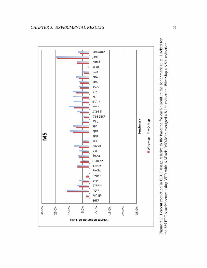
CHAPTER 5. EXPERIMENTAL RESULTS 51
-35.0%
-25.0%
-15.0%
-5.0%
5.0%
15.0%
25.0%
35.0%
s298
elliptic
ex5p
misex3
alu4
diffeq
bigkey
apex4
ex1010
tseng
seq
apex2
des
dsip
spla
pdc
frisc
s38584.1
s38417
clma
cfc18
cfc
iir1
oc54
rsd1
rsd2
cft8
desa
glue2
pajf
geomean
Percent Reduction of FLUTs
Be
nch
mar
k
M5
WireMap
MO-M
ap
Figu
re5.
2:Pe
rcen
tred
uctio
nin
FLU
Tus
age
rela
tive
toth
eba
selin
efo
rea
chci
rcui
tin
the
benc
hmar
ksu
ite.
Pack
edfo
rth
eM
5FP
GA
arch
itect
ure
usin
gV
PRw
ithA
APa
ck.M
O-M
apav
erag
eda
8.1%
redu
ctio
n,W
ireM
apa
6.8%
redu
ctio
n.

CHAPTER 5. EXPERIMENTAL RESULTS 52
-35.0%
-25.0%
-15.0%
-5.0%
5.0%
15.0%
25.0%
35.0%
s298
elliptic
ex5p
misex3
alu4
diffeq
bigkey
apex4
ex1010
tseng
seq
apex2
des
dsip
spla
pdc
frisc
s38584.1
s38417
clma
cfc18
cfc
iir1
oc54
rsd1
rsd2
cft8
desa
glue2
pajf
geomean
Percent Reduction of FLUTs
Be
nch
mar
k
M6
WireMap
MO-M
ap
Figu
re5.
3:Pe
rcen
tred
uctio
nin
FLU
Tus
age
rela
tive
toth
eba
selin
efo
rea
chci
rcui
tin
the
benc
hmar
ksu
ite.
Pack
edfo
rth
eM
6FP
GA
arch
itect
ure
usin
gV
PRw
ithA
APa
ck.M
O-M
apav
erag
eda
9.5%
redu
ctio
n,W
ireM
apa
9.3%
redu
ctio
n.

CHAPTER 5. EXPERIMENTAL RESULTS 53
-35.0%
-25.0%
-15.0%
-5.0%
5.0%
15.0%
25.0%
35.0%
s298
elliptic
ex5p
misex3
alu4
diffeq
bigkey
apex4
ex1010
tseng
seq
apex2
des
dsip
spla
pdc
frisc
s38584.1
s38417
clma
cfc18
cfc
iir1
oc54
rsd1
rsd2
cft8
desa
glue2
pajf
geomean
Percent Reduction of FLUTs
Be
nch
mar
k
M7
WireMap
MO-M
ap
Figu
re5.
4:Pe
rcen
tred
uctio
nin
FLU
Tus
age
rela
tive
toth
eba
selin
efo
rea
chci
rcui
tin
the
benc
hmar
ksu
ite.
Pack
edfo
rth
eM
7FP
GA
arch
itect
ure
usin
gV
PRw
ithA
APa
ck.M
O-M
apav
erag
eda
10.6
%re
duct
ion,
Wir
eMap
a9.
9%re
duct
ion.

CHAPTER 5. EXPERIMENTAL RESULTS 54
-35.0%
-25.0%
-15.0%
-5.0%
5.0%
15.0%
25.0%
35.0%
s298
elliptic
ex5p
misex3
alu4
diffeq
bigkey
apex4
ex1010
tseng
seq
apex2
des
dsip
spla
pdc
frisc
s38584.1
s38417
clma
cfc18
cfc
iir1
oc54
rsd1
rsd2
cft8
desa
glue2
pajf
geomean
Percent Reduction of FLUTs
Be
nch
mar
k
M8
WireMap
MO-M
ap
Figu
re5.
5:Pe
rcen
tred
uctio
nin
FLU
Tus
age
rela
tive
toth
eba
selin
efo
rea
chci
rcui
tin
the
benc
hmar
ksu
ite.
Pack
edfo
rth
eM
8FP
GA
arch
itect
ure
usin
gV
PRw
ithA
APa
ck.M
O-M
apav
erag
eda
9.9%
redu
ctio
n,W
ireM
apa
9.3%
redu
ctio
n.

CHAPTER 5. EXPERIMENTAL RESULTS 55
-35.0%
-25.0%
-15.0%
-5.0%
5.0%
15.0%
25.0%
35.0%
s298
elliptic
ex5p
misex3
alu4
diffeq
bigkey
apex4
ex1010
tseng
seq
apex2
des
dsip
spla
pdc
frisc
s38584.1
s38417
clma
cfc18
cfc
iir1
oc54
rsd1
rsd2
cft8
desa
glue2
pajf
geomean
Percent Reduction of ALMs
Be
nch
mar
k
Stra
tix
II
WireMap
MO-M
ap
Figu
re5.
6:Pe
rcen
tred
uctio
nin
AL
Mus
age
rela
tive
toth
eba
selin
efo
rea
chci
rcui
tin
the
benc
hmar
ksu
ite.
Pack
edfo
rth
eSt
ratix
IIFP
GA
arch
itect
ure
usin
gQ
uart
usII
.MO
-Map
aver
aged
a8.
3%re
duct
ion,
Wir
eMap
a7.
5%re
duct
ion.

CHAPTER 5. EXPERIMENTAL RESULTS 56
Table 5.2 summarizes the results of Figures 5.2, 5.3, 5.4, and 5.5 by presenting the
geometric mean of the benchmark suite’s FLUT usage and the percent reduction of FLUTs
compared to the ClassicMap results. For the Stratix II architecture row of Table 5.2, we are
comparing ALM usage as opposed to FLUTs. Data for each individual benchmark circuit
is included in Appendix A.
Table 5.2: FLUT utilization for each tech-mapper/architecture combination. The “PercentReduction” columns are the percent reduction in FLUTs calculated with respect to theBaseline mapping of an architecture.
ClassicMap WireMap MO-Map(Baseline)
Architecture FLUTs FLUTs Percent FLUTs Percent(ALMs) (ALMs) Reduction (ALMs) Reduction
M5 756.87 705.69 6.8% 695.41 8.1%M6 691.73 627.44 9.3% 625.75 9.5%M7 662.04 596.31 9.9% 591.72 10.6%M8 656.16 595.30 9.3% 590.93 9.9%
Stratix II 651.14 602.26 7.5% 597.35 8.3%
On average, with respect to ClassicMap, WireMap reduces FLUT usage by 6.8% to
9.9%, depending on academic architecture, and reduces ALM utilization by 7.5% for the
Stratix II. These FLUT reductions are comparable to the 6.3% reduction reported in previ-
ous work [6]. The differences between our experimental setup and that of the previous work
(different FPGA architecture, different synthesis procedure, different benchmark suite cir-
cuits, and a priority cuts tech-mapper versus a complete cut enumeration tech-mapper) can
be used to explain the differences between our results.
WireMap mappings pack into the same or fewer FLUTs than the equivalent ClassicMap
mappings for every benchmark packed for an academic architecture. For the Stratix II ar-
chitecture, WireMap only does worse than ClassicMap for the “elliptic” benchmark, where

CHAPTER 5. EXPERIMENTAL RESULTS 57
the WireMap mapping packs into 9 more ALMs than the ClassicMap mapping. To explain
this discrepancy, we first note that “elliptic” has a large proportion of 6-LUTs in its map-
pings, 212 6-LUTs out of 319 total LUTs for WireMap and 225 6-LUTs out of 318 total
LUTs for ClassicMap. We then examine the Quartus II packings and see that a great many
of these 6-LUTs are packed together into ALMs, 65 dual 6-LUT ALMs for WireMap and
71 for ClassicMap. Recall that two 6-LUTs can be packed into a single Stratix II ALM
providing that both 6-LUTs have identical truth tables and that our FLUTs in the academic
FPGA architectures do not have this feature. It appears that for the “elliptic” benchmark, a
great number of 6-LUTs that can take advantage of the extra features of a Stratix II ALM
are included in the mapping. Therefore, WireMap’s tendency to reduce the number of 6-
LUTs is ineffective at reducing FLUT usage because many of the 6-LUTs can be packed
into ALMs together.
MO-Map shows greater average FLUT and ALM reductions than WireMap, between
8.1% to 10.6% for the academic architectures and 8.3% for the Stratix II. However, for
some benchmark circuits MO-Map produces a worse result than the baseline. Of particular
note is the benchmark “dsip”. MO-Map has very poor results for “dsip” when packing for
the M7, M8, and Stratix II architectures, doing 28.5% to 32.6% worse than ClassicMap.
We hypothesize that the repeated used of the Exact Area algorithm during MO-Maps extra
area recovery step is the cause. The Exact Area algorithm optimizes area locally for a given
node, it does not optimize for the global area problem. It seems likely that the superior
solution found by ClassicMap and WireMap is never found by MO-Map due to MO-Map
getting stuck in a local minima of the solution space due to repeated use of MO-Map’s
greedy area recovery step.
In summary, MO-Map reduces average FLUT usage with respect to the baseline by

CHAPTER 5. EXPERIMENTAL RESULTS 58
0.2% to 1.3% (depending on architecture) more than WireMap when LUT balancing is
disabled. Although there is a small average FLUT reduction, the greedy nature of MO-
Map’s extra area recovery step leads to poor results for specific benchmarks.
5.2 LUT Balancing Experiments
In this section, we present our experimental results when LUT balancing is used during the
mapping process. We performed two sets of experiments with our LUT balancing scheme,
which were described in Section 4.1. In the first set, the benchmark suite is mapped with
varying values of Weight(6), ranging from 1.0 to 2.5 in 0.1 increments. In the second
set we vary both Weight(6) and Weight(5). For brevity, we will refer to these two sets of
experiments as the W6 experiments and the W5&6 experiments respectively.
5.2.1 Technology Mapping Results
We will begin by presenting the LUT distributions of the W6 experiments mappings. Fig-
ures 5.7, 5.8, and 5.9 present the LUT distributions for the ClassicMap, WireMap, and
MO-Map tech-mappers respectively. The y-axes of the figures are the number of LUTs,
normalized to the baseline mapping (ClassicMap without LUT Balancing). The x-axes has
several categories for LUTs that use different numbers of their K inputs, and an additional
category labelled “Total LUTs’, which is the total number of LUTs. Each bar in an x-axis
category represents the sum total number of LUTs found in all of the benchmark suite cir-
cuit’s mappings, normalized to the baseline. Each bar colour corresponds to the Weight(6)
value used to perform the tech-mapping. The data used to create these figures is presented
in tabular form in Appendix B.
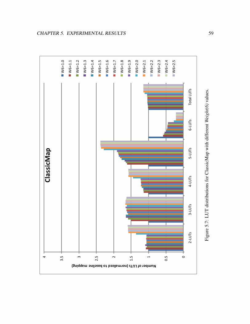
CHAPTER 5. EXPERIMENTAL RESULTS 59
0
0.51
1.52
2.53
3.54
2-L
UTs
3-L
UTs
4-L
UTs
5-L
UTs
6-L
UTs
Tota
l LU
Ts
Number of LUTs (normalized to baseline mapping)
Cla
ssic
Map
W6
=1
.0
W6
=1
.1
W6
=1
.2
W6
=1
.3
W6
=1
.4
W6
=1
.5
W6
=1
.6
W6
=1
.7
W6
=1
.8
W6
=1
.9
W6
=2
.0
W6
=2
.1
W6
=2
.2
W6
=2
.3
W6
=2
.4
W6
=2
.5
Figu
re5.
7:L
UT
dist
ribu
tions
forC
lass
icM
apw
ithdi
ffer
entW
eigh
t(6)
valu
es.

CHAPTER 5. EXPERIMENTAL RESULTS 60
0
0.51
1.52
2.53
3.54
2-L
UTs
3-L
UTs
4-L
UTs
5-L
UTs
6-L
UTs
Tota
l LU
Ts
Number of LUTs (normalized to baseline mapping)
Wir
eMap
W6
=1
.0
W6
=1
.1
W6
=1
.2
W6
=1
.3
W6
=1
.4
W6
=1
.5
W6
=1
.6
W6
=1
.7
W6
=1
.8
W6
=1
.9
W6
=2
.0
W6
=2
.1
W6
=2
.2
W6
=2
.3
W6
=2
.4
W6
=2
.5
Figu
re5.
8:L
UT
dist
ribu
tions
forW
ireM
apw
ithdi
ffer
entW
eigh
t(6)
valu
es.

CHAPTER 5. EXPERIMENTAL RESULTS 61
0
0.51
1.52
2.53
3.54
2-L
UTs
3-L
UTs
4-L
UTs
5-L
UTs
6-L
UTs
Tota
l LU
Ts
Number of LUTs (normalized to baseline mapping)
MO
-Map
W6
=1
.0
W6
=1
.1
W6
=1
.2
W6
=1
.3
W6
=1
.4
W6
=1
.5
W6
=1
.6
W6
=1
.7
W6
=1
.8
W6
=1
.9
W6
=2
.0
W6
=2
.1
W6
=2
.2
W6
=2
.3
W6
=2
.4
W6
=2
.5
Figu
re5.
9:L
UT
dist
ribu
tions
forM
O-M
apw
ithdi
ffer
entW
eigh
t(6)
valu
es.

CHAPTER 5. EXPERIMENTAL RESULTS 62
Analyzing Figures 5.7, 5.8, and 5.9 reveals several general trends. The most obvious
trend is that as Weight(6) increases, the number of 6-LUTs in the mappings decrease. This
is an expected result of raising Weight(6). Another expected trend observed, is that as
Weight(6) rises, the number of LUTs that use five or fewer inputs increases to compensate
for the missing 6-LUTs. Also, the total number of LUTs in the mapping, which is the
traditional measurement of mapping area, increases with Weight(6). The data used to create
these figures is presented in tabular form in Appendix B.
We note a large shift in the distribution when Weight(6) exceeds 2.0. At this point,
the number of LUTs that use five of fewer inputs and the total number of LUTs increases
drastically, while the number of 6-LUTs plummets. This effect occurs because we have
weighted a 6-LUT such that it is more expensive than two LUTs that both use five or less
inputs. As a result, it is typically favourable for the mapper to choose two smaller LUTs
over a single 6-LUT.
When comparing the distributions, we see that WireMap and MO-Map produce sim-
ilar results. When the WireMap and MO-Map distributions are compared to the Clas-
sicMap distribution, it can be seen that the ClassicMap distribution has more 5-LUTs, while
WireMap and MO-Map’s distributions have more 2-LUTs and 3-LUTs. This effect is at-
tributed to WireMap’s edge-recovery heuristics, which modifies the LUT distribution such
that LUTs with fewer inputs are favoured [6][5].
For all of our W6 experiments results, as Weight(6) increases, the number of 6-LUTs
drops while the number of 5-LUTs increases. In our next set of experiments, the W5&6
experiments, we modify the Weight(5) value as well as Weight(6). This is done to limit the
increase of 5-LUTs noted in the W6 experiments. 5-LUTs are the largest LUTs that can be
packed into a fractured mode FLUT, and are therefore the most likely to have packability

CHAPTER 5. EXPERIMENTAL RESULTS 63
issues. Figures 5.10, 5.11, and 5.12 present the LUT distributions of our W5&6 experi-
ments for ClassicMap, WireMap, and MO-Map respectively. These figures are presented
in an identical manner to the previous LUT distribution figures.
Examining Figures 5.10, 5.11, and 5.12 relative to Figures 5.7, 5.8, and 5.9 shows that
the average number of 5-LUTs included in the mappings of all tech-mappers has decreased
now that Weight(5) is greater than 1.0 and that the average number of 6-LUTs remained rel-
atively unchanged. The bars in the 5-LUT categories of Figures 5.10, 5.11, and 5.12 create
a “sawtooth” pattern. Each “tooth” in the 5-LUT category is formed due by several bars
side by side that have the same Weight(6) value and increasing Weight(5) values. The high
point of each “tooth” occurs when Weight(5) is at its smallest value for a given Weight(6).
The average number of 2-LUTs, 3-LUTs, and 4-LUTs increased to compensate for the
reduction of 5-LUTs. A less distinct version of the “sawtooth” pattern observed in the
5-LUT category is present in the 2-LUT, 3-LUT, and 4-LUT categories. The high point
of a “tooth” in these smaller LUT categories tends to coincide with the highest values
of Weight(5) for a given Weight(6), a trend opposite to that seen in the 5-LUT category.
This shows that more 2-LUTs, 3-LUTs, and 4-LUTs are being used to compensate for the
reduced number of 5-LUTs when a high Weight(5) values is specified.
Previously, in the W6 experiments, the ClassicMap LUT distribution compensated for
fewer 6-LUTs primarily with a large increase in 5-LUTs, whereas WireMap and MO-Map
compensated by increasing the occurrence of all smaller LUT sizes. Increasing Weight(5)
above 1.0 in the W5&6 experiments has forced the ClassicMap LUT distribution to become
more similar to that of WireMap and MO-Map, where 3-LUTs and 4-LUTs occur more
frequently to make up for the lack of 5-LUTs and 6-LUTs. Despite the similarity in 5-LUT
and 6-LUT numbers, there are still notable differences between the different tech-mapper

CHAPTER 5. EXPERIMENTAL RESULTS 64
0
0.51
1.52
2.53
3.54
2-L
UTs
3-L
UTs
4-L
UTs
5-L
UTs
6-L
UTs
Tota
l LU
Ts
Number of LUTs (normalized to baseline mapping)
Cla
ssic
Map
W6
=1
.2, W
5=
1.1
W6
=1
.4, W
5=
1.1
W6
=1
.4, W
5=
1.2
W6
=1
.4, W
5=
1.3
W6
=1
.6, W
5=
1.1
W6
=1
.6, W
5=
1.2
W6
=1
.6, W
5=
1.3
W6
=1
.6, W
5=
1.4
W6
=1
.8, W
5=
1.1
W6
=1
.8, W
5=
1.2
W6
=1
.8, W
5=
1.4
W6
=1
.8, W
5=
1.6
W6
=2
.0, W
5=
1.1
W6
=2
.0, W
5=
1.2
W6
=2
.0, W
5=
1.6
W6
=2
.4, W
5=
1.1
W6
=2
.4, W
5=
1.2
W6
=2
.4, W
5=
1.6
W6
=2
.4, W
5=
2.0
Figu
re5.
10:L
UT
dist
ribu
tions
forC
lass
icM
apw
ithva
ryin
gW
eigh
t(5)
and
Wei
ght(
6).

CHAPTER 5. EXPERIMENTAL RESULTS 65
0
0.51
1.52
2.53
3.54
2-L
UTs
3-L
UTs
4-L
UTs
5-L
UTs
6-L
UTs
Tota
l LU
Ts
Number of LUTs (normalized to baseline mapping)
Wir
eMap
W6
=1
.2, W
5=
1.1
W6
=1
.4, W
5=
1.1
W6
=1
.4, W
5=
1.2
W6
=1
.4, W
5=
1.3
W6
=1
.6, W
5=
1.1
W6
=1
.6, W
5=
1.2
W6
=1
.6, W
5=
1.3
W6
=1
.6, W
5=
1.4
W6
=1
.8, W
5=
1.1
W6
=1
.8, W
5=
1.2
W6
=1
.8, W
5=
1.4
W6
=1
.8, W
5=
1.6
W6
=2
.0, W
5=
1.1
W6
=2
.0, W
5=
1.2
W6
=2
.0, W
5=
1.6
W6
=2
.4, W
5=
1.1
W6
=2
.4, W
5=
1.2
W6
=2
.4, W
5=
1.6
W6
=2
.4, W
5=
2.0
Figu
re5.
11:L
UT
dist
ribu
tions
forW
ireM
apw
ithva
ryin
gW
eigh
t(5)
and
Wei
ght(
6).

CHAPTER 5. EXPERIMENTAL RESULTS 66
0
0.51
1.52
2.53
3.54
2-L
UTs
3-L
UTs
4-L
UTs
5-L
UTs
6-L
UTs
Tota
l LU
Ts
Number of LUTs (normalized to baseline mapping)
MO
-Map
W6
=1
.2, W
5=
1.1
W6
=1
.4, W
5=
1.1
W6
=1
.4, W
5=
1.2
W6
=1
.4, W
5=
1.3
W6
=1
.6, W
5=
1.1
W6
=1
.6, W
5=
1.2
W6
=1
.6, W
5=
1.3
W6
=1
.6, W
5=
1.4
W6
=1
.8, W
5=
1.1
W6
=1
.8, W
5=
1.2
W6
=1
.8, W
5=
1.4
W6
=1
.8, W
5=
1.6
W6
=2
.0, W
5=
1.1
W6
=2
.0, W
5=
1.2
W6
=2
.0, W
5=
1.6
W6
=2
.4, W
5=
1.1
W6
=2
.4, W
5=
1.2
W6
=2
.4, W
5=
1.6
W6
=2
.4, W
5=
2.0
Figu
re5.
12:L
UT
dist
ribu
tions
forM
O-M
apw
ithva
ryin
gW
eigh
t(5)
and
Wei
ght(
6).

CHAPTER 5. EXPERIMENTAL RESULTS 67
LUT distributions. WireMap and MO-Map have higher numbers of the smaller 2-LUTs
and 3-LUTs, while ClassicMap has more 4-LUTs and slightly fewer LUTs overall. This is
a change from when LUT balancing was not used and MO-Map mappings had the fewest
number of LUTs overall. MO-Map still has fewer total LUTs than WireMap.
5.2.2 Packing Results
In this subsection, we present the FLUT usage data obtained from packing the mappings
of our LUT balancing experiments. Figure 5.13 contains four sub-figures, one for each
academic architecture, graphing the FLUT usage of the W6 experiments. Packing was
performed with VPR’s AAPack [7][8]. Due to space constraints, the FLUT usage for each
individual circuit is not given. Instead, each data point is the benchmark suites geometric
mean of FLUT usage when the suite is mapped with a given Weight(6) value. There are five
lines in each of the subfigures. Three of the lines, ClassicMap, WireMap, and MO-Map,
correspond with the left y-axis and give the average FLUT utilizations. The remaining
two lines, (ClassicMap - MO-Map) and (WireMap - MO-Map), are measured against the
right y-axis and give the difference in FLUT usage with respect to MO-Map. Figure 5.14
provides an equivalent graph detailing average ALM usage resulting from the Quartus II
packings. Note that the left y-axes of the figures start at 500 to provide better resolution.
The right y-axes of the figures all have a range of 200, but the endpoints of the range are
varied to provide sufficient spacing between the lines on the graph for the purpose of clarity.
The data used to create these graphs is included in tabular format in Appendix C.
Figures 5.13 and 5.14 include the packing results from Section 5.1.2, where no LUT
balancing was performed, for reference. These are the Weight(6) 1.0 data points and the
ClassicMap point is our baseline for comparison. As was noted in Section 5.1.2, WireMap

CHAPTER 5. EXPERIMENTAL RESULTS 68
-40.0
-20.0
0.0
20.0
40.0
60.0
80.0
100.0
120.0
140.0
160.0
500
550
600
650
700
750
800
1.0
1.1
1.2
1.3
1.4
1.5
1.6
1.7
1.8
1.9
2.0
2.1
2.2
2.3
2.4
2.5
FLU
T D
iffe
ren
ce
FLU
Ts
Weight(6)
M5
ClassicMap WireMap MO-Map
(ClassicMap - MO-Map) (WireMap - MO-Map)
(a) M5 Architecture.
-120.0
-100.0
-80.0
-60.0
-40.0
-20.0
0.0
20.0
40.0
60.0
80.0
500
550
600
650
700
750
800
1.0
1.1
1.2
1.3
1.4
1.5
1.6
1.7
1.8
1.9
2.0
2.1
2.2
2.3
2.4
2.5
FLU
T D
iffe
ren
ce
FLU
TsWeight(6)
M6
ClassicMap WireMap MO-Map
(ClassicMap - MO-Map) (WireMap - MO-Map)
(b) M6 Architecture.
-120.0
-100.0
-80.0
-60.0
-40.0
-20.0
0.0
20.0
40.0
60.0
80.0
500
550
600
650
700
750
800
1.0
1.1
1.2
1.3
1.4
1.5
1.6
1.7
1.8
1.9
2.0
2.1
2.2
2.3
2.4
2.5
FLU
T D
iffe
ren
ce
FLU
Ts
Weight(6)
M7
ClassicMap WireMap MO-Map
(ClassicMap - MO-Map) (WireMap - MO-Map)
(c) M7 Architecture.
-120.0
-100.0
-80.0
-60.0
-40.0
-20.0
0.0
20.0
40.0
60.0
80.0
500
550
600
650
700
750
800
1.0
1.1
1.2
1.3
1.4
1.5
1.6
1.7
1.8
1.9
2.0
2.1
2.2
2.3
2.4
2.5
FLU
T D
iffe
ren
ce
FLU
Ts
Weight(6)
M8
ClassicMap WireMap MO-Map
(ClassicMap - MO-Map) (WireMap - MO-Map)
(d) M8 Architecture.
Figure 5.13: Academic architecture FLUT resource utilizations post-packing. Mapping isperformed with the three tech-mappers and varyied values of Weight(6). Subfigures (a),(b), (c) and (d) correspond to one of the four academic FGPA architectures.

CHAPTER 5. EXPERIMENTAL RESULTS 69
-120
-100
-80
-60
-40
-20
0
20
40
60
80
500
550
600
650
700
750
800
1.0
1.1
1.2
1.3
1.4
1.5
1.6
1.7
1.8
1.9
2.0
2.1
2.2
2.3
2.4
2.5
ALM
Dif
fere
nce
ALM
s
Weight(6)
Stratix II
ClassicMap WireMap MO-Map
(ClassicMap - MO-Map) (WireMap - MO-Map)
(a) Stratix II.
-120.0
-100.0
-80.0
-60.0
-40.0
-20.0
0.0
20.0
40.0
60.0
80.0
500
550
600
650
700
750
800
1.0
1.1
1.2
1.3
1.4
1.5
1.6
1.7
1.8
1.9
2.0
2.1
2.2
2.3
2.4
2.5
FLU
T D
iffe
ren
ce
FLU
Ts
Weight(6)
M8
ClassicMap WireMap MO-Map
(ClassicMap - MO-Map) (WireMap - MO-Map)
(b) M8 Architecture.
Figure 5.14: Stratix II ALM resource utilization after fitting. Mapping is performed withthe three tech-mappers and varied values of Weight(6). M8 architecture results repeated forcomparison purposes.
and MO-Map produce a significant reduction in FLUTs over the baseline when Weight(6) is
1.0. With the data of Figures 5.13 and 5.14 we can see that increasing Weight(6) to 1.1 pro-
duces a drastic reduction in average FLUT use for ClassicMap on all FPGA architectures.
MO-Map and WireMap also see benefits, but not to the same extent as ClassicMap.
After the initial jump from 1.0 to 1.1, there are only small variations in the tech-mappers
average FLUT usage until Weight(6) reaches 2.0. At that point, there is another significant
jump up. This corresponds to the increase in total number of LUTs we observed in the LUT
distributions of Section 5.2.1. For some of the architectures/tech-mapper combinations,
increasing Weight(6) beyond 2.0 can produce worse results than the 1.0 scenario. So we
can conclude that LUT balancing can be made too aggressive and negatively affect results.
For all architectures and Weight(6) values, MO-Map provides a greater average reduc-
tion in FLUT usage than either WireMap or ClassicMap. The average number of FLUTs in

CHAPTER 5. EXPERIMENTAL RESULTS 70
WireMap’s results are less than ClassicMap’s for the M5, M6, and M7 architectures, but are
almost identical for the M8 architecture and the Stratix II. The gap between average FLUT
usage for MO-Map and WireMap compared to ClassicMap gets smaller as M increases.
This is an indication of the greater freedom large M values give to the packing tool, which
allows for tighter mappings irregardless of LUT distribution. If M is large, then it becomes
easier to pack two LUTs together into a fractured mode FLUT because the input sharing
constraints are less stringent.
The difference in average FLUT count between ClassicMap and MO-Map varied from
5.1 to 70.3 FLUTs. The difference between WireMap and MO-Map varied from 1.7 to 12.3
FLUTs. We observe that the changing the Weight(6) value introduced significantly more
variability between the results of ClassicMap and MO-Map than it did for WireMap and
MO-Map.
Overall, the addition of LUT balancing provides benefits for all three tech-mappers.
The Weight(6) value that minimizes average FLUT usage varies with tech-mapper and ar-
chitecture, but is always between 1.1 and 2.0 in our results. MO-Map provides an incre-
mental improvement over WireMap. ClassicMap becomes comparable with WireMap for
a sufficiently large M value.
We will now consider the data from our W5&6 experiments. Figure 5.15 and Fig-
ure 5.16 are set up identically to Figure 5.13 and Figure 5.14, except that the x-axes list
both the Weight(6) and Weight(5) values used during technology mapping. The Weight(5)
values were selected after examining the data from our W6 experiments. The data used to
create these graphs is included in Appendix C in tabular format.
Examining Figures 5.15 and 5.16 shows that the W5&6 experiments data has some
similarities to the W6 experiments results. MO-Map shows small average FLUT reductions

CHAPTER 5. EXPERIMENTAL RESULTS 71
-40.0
-20.0
0.0
20.0
40.0
60.0
80.0
100.0
120.0
140.0
160.0
500
550
600
650
700
750
800
1.2
, 1.1
1.4
, 1.1
1.4
, 1.2
1.4
, 1.3
1.6
, 1.1
1.6
, 1.2
1.6
, 1.3
1.6
, 1.4
1.8
, 1.1
1.8
, 1.2
1.8
, 1.4
1.8
, 1.6
2.0
, 1.1
2.0
, 1.2
2.0
, 1.6
2.4
, 1.1
2.4
, 1.2
2.4
, 1.6
2.4
, 2.0
FLU
T D
iffe
ren
ce
FLU
Ts
Weight(6), Weight(5)
M5
ClassicMap WireMap MO-Map
(ClassicMap - MO-Map) (WireMap - MO-Map)
(a) M5 Architecture.
-100.0
-80.0
-60.0
-40.0
-20.0
0.0
20.0
40.0
60.0
80.0
100.0
500
550
600
650
700
750
800
1.2
, 1.1
1.4
, 1.1
1.4
, 1.2
1.4
, 1.3
1.6
, 1.1
1.6
, 1.2
1.6
, 1.3
1.6
, 1.4
1.8
, 1.1
1.8
, 1.2
1.8
, 1.4
1.8
, 1.6
2.0
, 1.1
2.0
, 1.2
2.0
, 1.6
2.4
, 1.1
2.4
, 1.2
2.4
, 1.6
2.4
, 2.0
FLU
T D
iffe
ren
ce
FLU
TsWeight(6), Weight(5)
M6
ClassicMap WireMap MO-Map
(ClassicMap - MO-Map) (WireMap - MO-Map)
(b) M6 Architecture.
-100.0
-80.0
-60.0
-40.0
-20.0
0.0
20.0
40.0
60.0
80.0
100.0
500
550
600
650
700
750
800
1.2
, 1.1
1.4
, 1.1
1.4
, 1.2
1.4
, 1.3
1.6
, 1.1
1.6
, 1.2
1.6
, 1.3
1.6
, 1.4
1.8
, 1.1
1.8
, 1.2
1.8
, 1.4
1.8
, 1.6
2.0
, 1.1
2.0
, 1.2
2.0
, 1.6
2.4
, 1.1
2.4
, 1.2
2.4
, 1.6
2.4
, 2.0
FLU
T D
iffe
ren
ce
FLU
Ts
Weight(6), Weight(5)
M7
ClassicMap WireMap MO-Map
(ClassicMap - MO-Map) (WireMap - MO-Map)
(c) M7 Architecture.
-100.0
-80.0
-60.0
-40.0
-20.0
0.0
20.0
40.0
60.0
80.0
100.0
500
550
600
650
700
750
800
1.2
, 1.1
1.4
, 1.1
1.4
, 1.2
1.4
, 1.3
1.6
, 1.1
1.6
, 1.2
1.6
, 1.3
1.6
, 1.4
1.8
, 1.1
1.8
, 1.2
1.8
, 1.4
1.8
, 1.6
2.0
, 1.1
2.0
, 1.2
2.0
, 1.6
2.4
, 1.1
2.4
, 1.2
2.4
, 1.6
2.4
, 2.0
FLU
T D
iffe
ren
ce
FLU
Ts
Weight(6), Weight(5)
M8
ClassicMap WireMap MO-Map
(ClassicMap - MO-Map) (WireMap - MO-Map)
(d) M8 Architecture.
Figure 5.15: Academic architecture FLUT resource utilizations post-packing. Mappingis performed with the three tech-mappers and varyied values of Weight(5) and Weight(6).Subfigures (a), (b), (c) and (d) correspond to one of the four academic FGPA architectures.

CHAPTER 5. EXPERIMENTAL RESULTS 72
-100
-80
-60
-40
-20
0
20
40
60
80
100
500
550
600
650
700
750
800
1.2
, 1.1
1.4
, 1.1
1.4
, 1.2
1.4
, 1.3
1.6
, 1.1
1.6
, 1.2
1.6
, 1.3
1.6
, 1.4
1.8
, 1.1
1.8
, 1.2
1.8
, 1.4
1.8
, 1.6
2.0
, 1.1
2.0
, 1.2
2.0
, 1.6
2.4
, 1.1
2.4
, 1.2
2.4
, 1.6
2.4
, 2.0
ALM
Dif
fere
nce
ALM
s
Weight(6), Weight(5)
Stratix II
ClassicMap WireMap MO-Map
(ClassicMap - MO-Map) (WireMap - MO-Map)
(a) Stratix II.
-100.0
-80.0
-60.0
-40.0
-20.0
0.0
20.0
40.0
60.0
80.0
100.0
500
550
600
650
700
750
800
1.2
, 1.1
1.4
, 1.1
1.4
, 1.2
1.4
, 1.3
1.6
, 1.1
1.6
, 1.2
1.6
, 1.3
1.6
, 1.4
1.8
, 1.1
1.8
, 1.2
1.8
, 1.4
1.8
, 1.6
2.0
, 1.1
2.0
, 1.2
2.0
, 1.6
2.4
, 1.1
2.4
, 1.2
2.4
, 1.6
2.4
, 2.0
FLU
T D
iffe
ren
ce
FLU
Ts
Weight(6), Weight(5)
M8
ClassicMap WireMap MO-Map
(ClassicMap - MO-Map) (WireMap - MO-Map)
(b) M8 Architecture.
Figure 5.16: Stratix II ALM resource utilization after fitting. Mapping is performed withthe three tech-mappers and varied values of Weight(5) and Weight(6). M8 architectureresults repeated for comparison purposes.
over WireMap and ClassicMap in the majority of cases. Although, there are a few instances
in the M7, M8, and Stratix II data where MO-Map performs equal to or slightly worse than
ClassicMap or WireMap. WireMap reduces average FLUT usage over ClassicMap for M5,
M6, and M7, but produces equivalent results for M8 and the Stratix II architectures.
We note a “sawtooth” pattern in our results, each “tooth” of the saw corresponding to
Weight(5) varying while Weight(6) remains constant. In the M7, M8 and Stratix II architec-
tures, for a given Weight(6), low values of Weight(5) produce smaller numbers of FLUTs.
In contrast, for the M5 architecture the opposite is true, values of Weight(5) close to that
of Weight(6) produce the best results. For the M6 architecture, the difference between
different Weight(5) values is minimal.
Our results suggest that the appropriate Weight(5) value is related to the FLUT param-
eter M. For smaller M values, where a 5-LUT is more difficult to pack, the 5-LUT should

CHAPTER 5. EXPERIMENTAL RESULTS 73
be weighted more heavily, closer to the weighting of a 6-LUT, as the LUT distribution
produced can be packed more compactly into FLUTs. Conversely, large M values should
weight 5-LUTs equal to or slightly more than a smaller LUT because 5-LUTs can be packed
more easily in these architectures. There does not appear to be a benefit to replacing many
5-LUTs with smaller LUTs for architectures with large M values.
Comparing the W6 experiments data to the W5&6 experiments data, we find that a
superior average FLUT reduction can be achieved for the M5 and M6 architecture when
Weight(5) is adjusted. For M7, the results are almost equal. And for M8 and Stratix II
leaving Weight(5) at 1.0 produces the lowest average FLUT (ALM) utilization. The LUT
balancing parameters that produced the fewest FLUTs (ALMs) are given in Table 5.3. An
entry is provided for each architecture/tech-mapper combination. The tech-mapper that
produced the greatest average FLUT reduction is highlighted in dark grey for each archi-
tecture. The tech-mapper that produced the smallest average FLUT reduction is highlighted
in light grey. The baseline mapping is also included for each architecture and the percent
reduction with respect to the baseline is provided.
In all cases, MO-Map provides the greatest percent reduction over the baseline map-
ping. However, MO-Map’s percent reduction relative to the baseline is only 0.7% to 1.4%
greater than that of the second best tech-mapper for an architecture. The tech-mapper
with the second best percent reduction relative to the baseline varies with the architecture.
WireMap reduces average FLUT usage more than ClassicMap for the M5, M6, and M7 ar-
chitectures, but does not produce a superior reduction for the M8 architecture or the Stratix
II.
Overall, once an appropriate LUT balancing scheme is included, there is little difference
between the different tech-mappers in terms of FLUT minimization. Unfortunately, finding

CHAPTER 5. EXPERIMENTAL RESULTS 74
Table 5.3: LUT balancing Weight(6) and Weight(5) values that minimized average FLUTutilization for each tech-mapper/architecture combination.
Architecture Mapper Weight(6) Weight(5) FLUTs Percent Reduction(ALMs)
M5
Baseline 1.0 1.0 756.9 N/AClassicMap 1.6 1.4 705.0 6.9%WireMap 1.4 1.3 689.1 9.0%MO-Map 1.4 1.3 683.8 9.7%
M6
Baseline 1.0 1.0 691.7 N/AClassicMap 1.6 1.2 620.1 10.3%WireMap 1.6 1.2 606.8 12.3%MO-Map 2.4 1.6 599.7 13.3%
M7
Baseline 1.0 1.0 662.0 N/AClassicMap 2.0 1.1 568.4 14.1%WireMap 1.8 1.0 557.4 15.8%MO-Map 1.9 1.0 548.2 17.2%
M8
Baseline 1.0 1.0 656.2 N/AClassicMap 2.0 1.0 550.4 16.1%WireMap 2.0 1.0 554.7 15.5%MO-Map 1.9 1.0 544.5 17.0%
Stratix II
Baseline 1.0 1.0 651.1 N/AClassicMap 2.0 1.0 570.6 12.4%WireMap 1.6 1.0 571.0 12.3%MO-Map 2.0 1.0 561.5 13.8%
the best LUT balancing weight values is achieved through trial and error with a given
architecture/tech-mapper. The percent reduction of average FLUT usage relative to the
baseline for all LUT balancing parameters, architectures, and tech-mappers is included in
Appendix C.

CHAPTER 5. EXPERIMENTAL RESULTS 75
5.3 Placement and Routing Results
In this section, we present the maximum operating frequency (Fmax) data from the Quartus
II portion of our experiments targeting the Stratix II. In addition, we present the minimum
channel width and wirelength results from VPR’s placement and routing operations for the
academic FPGA architectures. No maximum operating frequency is provided for the VPR
results because the version of VPR with AAPack that we use in our experiments is not
timing-driven.
5.3.1 Maximum Operating Frequency
Figure 5.17(a) and 5.17(b) show the maximum operating frequency reported by Quartus
II for the W6 experiments and W5&6 experiments respectively. The number reported is
the geometric mean of the benchmark suite circuit’s maximum operating frequency. Only
designs containing flip-flops reported a maximum operating frequency in the Quartus II
timing analyzer log, so only those design’s maximum operating frequencies are included
in the calculation. In our benchmark suite, twenty out of the thirty benchmarks contained
flip-flops. The y-axes of the figures list the maximum operating frequency in MHz. The
x-axes show the weight parameters used for LUT balancing. There are three lines on each
graph corresponding to the three tech-mappers. The data is presented in tabular format in
Appendix F
Noting the very small range on the y-axis, we observe that the maximum operating
frequency does not change significantly for any of our different mappings. The average
maximum operating frequency remained between 190 and 196 MHz for all variants of our
technology mapping parameters. At first, this data indicates that packing a design into

CHAPTER 5. EXPERIMENTAL RESULTS 76
184
186
188
190
192
194
196
198
200
1.0
1.1
1.2
1.3
1.4
1.5
1.6
1.7
1.8
1.9
2.0
2.1
2.2
2.3
2.4
2.5
Max
imu
m O
pe
rati
ng
Fre
qu
en
cy (
MH
z)
Weight(6)
ClassicMap WireMap MO-Map
(a) Data for varying Weight(6) mappings.
184
186
188
190
192
194
196
198
200
1.2
, 1.1
1.4
, 1.1
1.4
, 1.2
1.4
, 1.3
1.6
, 1.1
1.6
, 1.2
1.6
, 1.3
1.6
, 1.4
1.8
, 1.1
1.8
, 1.2
1.8
, 1.4
1.8
, 1.6
2.0
, 1.1
2.0
, 1.2
2.0
, 1.6
2.4
, 1.1
2.4
, 1.2
2.4
, 1.6
2.4
, 2.0Max
imu
m O
pe
rati
ng
Fre
qu
en
cy (
MH
z)
Weight(6), Weight(5)
ClassicMap WireMap MO-Map
(b) Data for varying Weight(6) and Weight(5).
Figure 5.17: Average maximum operating frequency reported by Quartus II.

CHAPTER 5. EXPERIMENTAL RESULTS 77
fewer ALMs does not have a significant impact on circuit speed. However, we set several
flags in the Quartus II software that instruct the CAD tools to optimize for area. Therefore,
we expect that an increase in maximum operating frequency is possible with different tool
settings. Further experimentation is necessary before concrete conclusions can be drawn.
Another caveat is that our benchmark suite is ill-suited for a maximum operating fre-
quency analysis. Of the 30 benchmark circuits, only 20 have flip-flops and contribute
towards our geometric mean. And of these 20, three circuits have such simplistic sequen-
tial components that their maximum operating frequency tops out at 500 MHz, the highest
frequency that Quartus II optimizes for on the Stratix II without a specific maximum oper-
ating frequency target. Such circuits are too trivial for a meaningful critical path benchmark
suite.
5.3.2 Minimum Channel Width and Wirelength
We are using an alpha version of the new VPR with AAPack software to place and route
circuits on our academic FPGA architectures. This alpha software does not have a timing-
driven mode, and thus does not provide a critical path estimate for a successfully routed
circuit. We collected data from the placement and routing phases, including the minimum
channel width and the total wirelength required to route a circuit, to provide some insight
on the routing ramifications when packing designs into fewer FLUTs.
The minimum channel width is the minimum number of tracks in each routing channel
on the FPGA that allowed for a successful routing of the circuit. VPR iteratively routes
the design with different channel widths to search for this minimum. Wirelength is the
total number of routing resources used to route a circuit and is expressed in units of “CLBs
spanned”. Wire segments can span more than one CLB. This unit keeps the wirelength

CHAPTER 5. EXPERIMENTAL RESULTS 78
metric independent from the physical length of wire segments in an FPGA architecture.
In our placement and routing runs, neither the size of the FPGA’s CLB grid nor its rout-
ing channel width is fixed. This allows the FPGA to “grow” and provide enough resources
to accommodate any circuit. A consequence of this “growth” circuits that packed into
fewer FLUTs are placed onto a smaller FPGA Logic Block grid because fewer resources
are required.
Figures 5.18 and 5.19 graph the geometric mean of the benchmark suite circuit’s min-
imum channel width for the different architecture/tech-mapper combinations for the W6
experiments and W5&6 experiments data respectively. In a similar fashion, Figures 5.20
and 5.21 present the wirelength data for the W6 experiments and W5&6 experiments data.
The minimum channel width data is available in tabular format in Appendix D, and the
Wirelegnth data in Appendix E.
While performing routing for the smallest benchmark in our suite, “s298”, VPR would
sometimes quit with an error message. This error message would occur for some of the
mappings produced by all three of the tech-mappers. We have been unable to resolve this
error message, and so have excluded “s298” from all of the minimum channel width and
wirelength averages.

CHAPTER 5. EXPERIMENTAL RESULTS 79
25
27
29
31
33
35
37
1.0
1.1
1.2
1.3
1.4
1.5
1.6
1.7
1.8
1.9
2.0
2.1
2.2
2.3
2.4
2.5
Min
imu
m C
han
ne
l W
idth
Weight(6)
M5
ClassicMap WireMap MO-Map
(a) M5 Architecture.
25
27
29
31
33
35
37
1.0
1.1
1.2
1.3
1.4
1.5
1.6
1.7
1.8
1.9
2.0
2.1
2.2
2.3
2.4
2.5
Min
imu
m C
han
ne
l W
idth
Weight(6)
M6
ClassicMap WireMap MO-Map
(b) M6 Architecture.
25
27
29
31
33
35
37
1.0
1.1
1.2
1.3
1.4
1.5
1.6
1.7
1.8
1.9
2.0
2.1
2.2
2.3
2.4
2.5
Min
imu
m C
han
ne
l W
idth
Weight(6)
M7
ClassicMap WireMap MO-Map
(c) M7 Architecture.
25
27
29
31
33
35
37
1.0
1.1
1.2
1.3
1.4
1.5
1.6
1.7
1.8
1.9
2.0
2.1
2.2
2.3
2.4
2.5
Min
imu
m C
han
ne
l W
idth
Weight(6)
M8
ClassicMap WireMap MO-Map
(d) M8 Architecture.
Figure 5.18: Academic architecture minimum channel widths. Mapping is performed withthe three tech-mappers and varyied values of Weight(6). Subfigures (a), (b), (c) and (d)correspond to one of the four academic FGPA architectures.

CHAPTER 5. EXPERIMENTAL RESULTS 80
25
27
29
31
33
35
37
1.2
, 1.1
1.4
, 1.1
1.4
, 1.2
1.4
, 1.3
1.6
, 1.1
1.6
, 1.2
1.6
, 1.3
1.6
, 1.4
1.8
, 1.1
1.8
, 1.2
1.8
, 1.4
1.8
, 1.6
2.0
, 1.1
2.0
, 1.2
2.0
, 1.6
2.4
, 1.1
2.4
, 1.2
2.4
, 1.6
2.4
, 2.0
Min
imu
m C
han
ne
l W
idth
Weight(6), Weight(5)
M5
ClassicMap WireMap MO-Map
(a) M5 Architecture.
25
27
29
31
33
35
37
1.2
, 1.1
1.4
, 1.1
1.4
, 1.2
1.4
, 1.3
1.6
, 1.1
1.6
, 1.2
1.6
, 1.3
1.6
, 1.4
1.8
, 1.1
1.8
, 1.2
1.8
, 1.4
1.8
, 1.6
2.0
, 1.1
2.0
, 1.2
2.0
, 1.6
2.4
, 1.1
2.4
, 1.2
2.4
, 1.6
2.4
, 2.0
Min
imu
m C
han
ne
l W
idth
Weight(6), Weight(5)
M6
ClassicMap WireMap MO-Map
(b) M6 Architecture.
25
27
29
31
33
35
37
1.2
, 1.1
1.4
, 1.1
1.4
, 1.2
1.4
, 1.3
1.6
, 1.1
1.6
, 1.2
1.6
, 1.3
1.6
, 1.4
1.8
, 1.1
1.8
, 1.2
1.8
, 1.4
1.8
, 1.6
2.0
, 1.1
2.0
, 1.2
2.0
, 1.6
2.4
, 1.1
2.4
, 1.2
2.4
, 1.6
2.4
, 2.0
Min
imu
m C
han
ne
l W
idth
Weight(6), Weight(5)
M7
ClassicMap WireMap MO-Map
(c) M7 Architecture.
25
27
29
31
33
35
37
1.2
, 1.1
1.4
, 1.1
1.4
, 1.2
1.4
, 1.3
1.6
, 1.1
1.6
, 1.2
1.6
, 1.3
1.6
, 1.4
1.8
, 1.1
1.8
, 1.2
1.8
, 1.4
1.8
, 1.6
2.0
, 1.1
2.0
, 1.2
2.0
, 1.6
2.4
, 1.1
2.4
, 1.2
2.4
, 1.6
2.4
, 2.0
Min
imu
m C
han
ne
l W
idth
Weight(6), Weight(5)
M8
ClassicMap WireMap MO-Map
(d) M8 Architecture.
Figure 5.19: Academic architecture minimum channel widths. Mapping is performed withthe three tech-mappers and varyied values of Weight(5) and Weight(6). Subfigures (a), (b),(c) and (d) correspond to one of the four academic FGPA architectures.

CHAPTER 5. EXPERIMENTAL RESULTS 81
30000
31000
32000
33000
34000
35000
36000
1.0
1.1
1.2
1.3
1.4
1.5
1.6
1.7
1.8
1.9
2.0
2.1
2.2
2.3
2.4
2.5
Wirelength
Weight(6)
M5
ClassicMap WireMap MO-Map
(a) M5 Architecture.
30000
31000
32000
33000
34000
35000
36000
1.0
1.1
1.2
1.3
1.4
1.5
1.6
1.7
1.8
1.9
2.0
2.1
2.2
2.3
2.4
2.5
Wirelength
Weight(6)
M6
ClassicMap WireMap MO-Map
(b) M6 Architecture.
30000
31000
32000
33000
34000
35000
36000
1.0
1.1
1.2
1.3
1.4
1.5
1.6
1.7
1.8
1.9
2.0
2.1
2.2
2.3
2.4
2.5
Wirelength
Weight(6)
M7
ClassicMap WireMap MO-Map
(c) M7 Architecture.
30000
31000
32000
33000
34000
35000
36000
1.0
1.1
1.2
1.3
1.4
1.5
1.6
1.7
1.8
1.9
2.0
2.1
2.2
2.3
2.4
2.5
Wirelength
Weight(6)
M8
ClassicMap WireMap MO-Map
(d) M8 Architecture.
Figure 5.20: Academic architecture wirelengths. Mapping is performed with the threetech-mappers and varyied values of Weight(6). Subfigures (a), (b), (c) and (d) correspondto one of the four academic FGPA architectures.

CHAPTER 5. EXPERIMENTAL RESULTS 82
30000
31000
32000
33000
34000
35000
36000
1.2
, 1.1
1.4
, 1.1
1.4
, 1.2
1.4
, 1.3
1.6
, 1.1
1.6
, 1.2
1.6
, 1.3
1.6
, 1.4
1.8
, 1.1
1.8
, 1.2
1.8
, 1.4
1.8
, 1.6
2.0
, 1.1
2.0
, 1.2
2.0
, 1.6
2.4
, 1.1
2.4
, 1.2
2.4
, 1.6
2.4
, 2.0
Wir
ele
ngt
h
Weight(6), Weight(5)
M5
ClassicMap WireMap MO-Map
(a) M5 Architecture.
30000
31000
32000
33000
34000
35000
36000
1.2
, 1.1
1.4
, 1.1
1.4
, 1.2
1.4
, 1.3
1.6
, 1.1
1.6
, 1.2
1.6
, 1.3
1.6
, 1.4
1.8
, 1.1
1.8
, 1.2
1.8
, 1.4
1.8
, 1.6
2.0
, 1.1
2.0
, 1.2
2.0
, 1.6
2.4
, 1.1
2.4
, 1.2
2.4
, 1.6
2.4
, 2.0
Wir
ele
ngt
hWeight(6), Weight(5)
M6
ClassicMap WireMap MO-Map
(b) M6 Architecture.
30000
31000
32000
33000
34000
35000
36000
1.2
, 1.1
1.4
, 1.1
1.4
, 1.2
1.4
, 1.3
1.6
, 1.1
1.6
, 1.2
1.6
, 1.3
1.6
, 1.4
1.8
, 1.1
1.8
, 1.2
1.8
, 1.4
1.8
, 1.6
2.0
, 1.1
2.0
, 1.2
2.0
, 1.6
2.4
, 1.1
2.4
, 1.2
2.4
, 1.6
2.4
, 2.0
Wir
ele
ngt
h
Weight(6), Weight(5)
M7
ClassicMap WireMap MO-Map
(c) M7 Architecture.
30000
31000
32000
33000
34000
35000
36000
1.2
, 1.1
1.4
, 1.1
1.4
, 1.2
1.4
, 1.3
1.6
, 1.1
1.6
, 1.2
1.6
, 1.3
1.6
, 1.4
1.8
, 1.1
1.8
, 1.2
1.8
, 1.4
1.8
, 1.6
2.0
, 1.1
2.0
, 1.2
2.0
, 1.6
2.4
, 1.1
2.4
, 1.2
2.4
, 1.6
2.4
, 2.0
Wir
ele
ngt
h
Weight(6), Weight(5)
M8
WireMap ClassicMap MO-Map
30000
31000
32000
33000
34000
35000
36000
1.2
, 1.1
1.4
, 1.1
1.4
, 1.2
1.4
, 1.3
1.6
, 1.1
1.6
, 1.2
1.6
, 1.3
1.6
, 1.4
1.8
, 1.1
1.8
, 1.2
1.8
, 1.4
1.8
, 1.6
2.0
, 1.1
2.0
, 1.2
2.0
, 1.6
2.4
, 1.1
2.4
, 1.2
2.4
, 1.6
2.4
, 2.0
Wir
ele
ngt
h
Weight(6), Weight(5)
M8
ClassicMap WireMap MO-Map
(d) M8 Architecture.
Figure 5.21: Academic architecture wirelengths. Mapping is performed with the threetech-mappers and varyied values of Weight(5) and Weight(6). Subfigures (a), (b), (c) and(d) correspond to one of the four academic FGPA architectures.

CHAPTER 5. EXPERIMENTAL RESULTS 83
In Table 5.4, we revisit the mappings that produced the greatest percent decrease in av-
erage FLUT usage with respect to the baseline for each academic FPGA architecture. This
data was previously presented in Table 5.3. We have added columns to the table stating
the average minimum channel width (column “MCW”) and wirelength for the benchmark
suite routings. There are also columns showing the percent difference in minimum channel
width and wirelength with respect to the baseline of the architecture. The tech-mapper that
produced the greatest average FLUT reduction is highlighted in dark grey for each architec-
ture. The tech-mapper that produced the smallest average FLUT reduction is highlighted
in light grey.
Intuitively, packing the same amount of logic into a smaller FPGA CLB grid will lead
to a higher density of routing resources, i.e. an increased minimum channel width. This
trend is observed in our results; a decrease in FLUT usage is accompanied by an increase
in minimum channel width ranging from 4.0% to 12.3% for our “best” mappings. We also
observe that wirelength decreases with decreasing FLUT usage anywhere from 3.6% to
11.2%. This can be explained by noting that if the CLB grid is smaller, the wires connecting
FLUTs together will not have to be as long to connect source to sink.

CHAPTER 5. EXPERIMENTAL RESULTS 84
Tabl
e5.
4:In
crea
sein
min
imum
chan
nel
wid
thfo
rth
ebe
nchm
ark
suite
pack
ings
that
have
the
grea
test
aver
age
FLU
Tm
inim
izat
ion.
Arc
hite
ctur
eTe
ch-M
appe
rW
6W
5FL
UT
FLU
TM
CW
MC
WW
irel
engt
hW
irel
engt
hPe
rcen
tPe
rcen
tPe
rcen
tR
educ
tion
Diff
eren
ceD
iffer
ence
M5
Bas
elin
e1.
01.
075
6.9
N/A
26.7
N/A
3551
4N
/AC
lass
icM
ap1.
61.
470
5.0
6.9%
27.9
4.3%
3296
3-7
.2%
Wir
eMap
1.4
1.3
689.
19.
0%28
.15.
1%32
576
-8.3
%M
O-M
ap1.
41.
368
3.8
9.7%
28.3
5.8%
3191
6-1
0.1%
M6
Bas
elin
e1.
01.
069
1.7
N/A
29.5
N/A
3469
7N
/AC
lass
icM
ap1.
61.
262
0.1
10.3
%30
.64.
0%32
797
-5.5
%W
ireM
ap1.
61.
260
6.8
12.3
%31
.77.
7%32
232
-7.1
%M
O-M
ap2.
41.
659
9.7
13.3
%33
.112
.3%
3342
1-3
.7%
M7
Bas
elin
e1.
01.
066
2.0
N/A
31.3
N/A
3467
6N
/AC
lass
icM
ap2.
01.
156
8.4
14.1
%33
.77.
6%32
268
-6.9
%W
ireM
ap1.
81.
055
7.4
15.8
%33
.88.
2%30
806
-11.
2%M
O-M
ap1.
91.
054
8.2
17.2
%34
.410
.1%
3110
4-1
0.3%
M8
Bas
elin
e1.
01.
065
6.2
N/A
31.8
N/A
3369
7N
/AC
lass
icM
ap2.
01.
055
0.4
16.1
%35
.411
.4%
3249
8-3
.6%
Wir
eMap
2.0
1.0
554.
715
.5%
34.7
9.3%
3241
2-3
.8%
MO
-Map
1.9
1.0
544.
517
.0%
34.8
9.5%
3176
3-5
.7%

CHAPTER 5. EXPERIMENTAL RESULTS 85
5.4 Estimating the Impact on Silicon Area
It is interesting to consider whether or not the decrease in FLUTs resource requirements
justifies the increase in minimum channel width. The programmable routing resources are
known to take up the majority of an FPGAs silicon area, approximately 65-75% of the total
die [11]. If we assume the remaining silicon area is used by logic resources, then we can
calculate the net change in silicon area. We estimate the percent change in silicon area for
our “best” mappings and present the data in Table 5.5.
To calculate the percent increase in silicon area due to the change in minimum channel
width we multiplied the percent increase in channel width from Table 5.4 by 0.65 and 0.75 .
Similarly, the FLUT percent decrease column of Table 5.4 was multiplied by 0.25 and 0.35
to estimate the percent decrease in silicon area due to FLUTs. Depending on architecture
and tech-mapper, we estimate that the percent increase in silicon area to be within -1.0%
to 5.9%. However, given how rough our estimation method is, and how close to zero the
percent increases are, it seems likely that these predicted changes to silicon area are within
the margin of error.

CHAPTER 5. EXPERIMENTAL RESULTS 86
Tabl
e5.
5:E
stim
ate
ofpe
rcen
tcha
nge
insi
licon
area
.
Arc
hite
ctur
eTe
ch-M
appe
rW
eigh
t(6)
Wei
ght(
5)Pe
rcen
tInc
reas
ePe
rcen
tDec
reas
eN
etSi
licon
InSi
licon
Are
aD
ueIn
Silic
onA
rea
Are
aPe
rcen
tTo
Rou
ting
Due
toFL
UT
sIn
crea
se
M5
Cla
ssic
Map
1.6
1.4
2.8-
3.2%
1.7-
2.4%
0.4-
1.5%
Wir
eMap
1.4
1.3
3.3-
3.8%
2.2-
3.1%
0.2-
1.6%
MO
-Map
1.4
1.3
3.8-
4.4%
2.4-
3.4%
0.4-
2.0%
M6
Cla
ssic
Map
1.6
1.2
2.6-
3.0%
2.6-
3.6%
(-1.
0)-0
.4%
Wir
eMap
1.6
1.2
5.0-
5.8%
3.1-
4.3%
0.7-
2.7%
MO
-Map
2.4
1.6
8.0-
9.2%
3.3-
4.7%
3.3-
5.9%
M7
Cla
ssic
Map
2.0
1.1
5.0-
5.7%
3.5-
5.0%
0.0-
2.2%
Wir
eMap
1.8
1.0
5.3-
6.2%
4.0-
5.5%
(-0.
2)-2
.2%
MO
-Map
1.9
1.0
6.5-
7.5%
4.3-
6.0%
0.5-
3.2%
M8
Cla
ssic
Map
2.0
1.0
7.4-
8.5%
4.0-
5.6%
1.8-
4.5%
Wir
eMap
2.0
1.0
6.0-
7.0%
3.9-
5.4%
0.6-
3.1%
MO
-Map
1.9
1.0
6.2-
7.1%
4.3-
6.0%
0.2-
2.9%

Chapter 6
Conclusions and Future Work
The FPGAs of vendors Xilinx and Altera feature fracturable look-up tables as the primary
component responsible for implementing Boolean logic. A FLUT has the ability to act as
a single large LUT, or two smaller LUTs with input-sharing restrictions. In FPGA technol-
ogy mapping, the area of a mapping is the number of LUTs included in the design. Such
a metric is inaccurate for modern FPGAs because of the difference in logic implementa-
tion capabilities of a FLUT versus a LUT. Therefore, technology mapping techniques that
minimize the number of FLUTs instead of LUTs are desirable.
6.1 Conclusions
In this thesis, we compared and evaluated three technology mapping algorithms, Clas-
sicMap, WireMap, and MO-Map. The evaluation was based upon which algorithm’s map-
pings packed into the smallest number of FLUTs, with the restriction that all mappings
had to maintain a minimum mapping depth. In the absence of LUT balancing, WireMap
mappings packed into an average of 6.8% to 9.9% fewer FLUTs than ClassicMap map-
87

CHAPTER 6. CONCLUSIONS AND FUTURE WORK 88
pings for our academic FPGA architectures and 7.5% fewer ALMs for the commercial
Stratix II architecture. MO-Map mappings, again in the absence of LUT balancing, packed
into an average of 8.1% to 10.6% fewer FLUTs than ClassicMap for the academic FPGA
architectures and 8.3% fewer ALMs for the Stratix II.
The effects of LUT balancing during technology mapping were also investigated. We
implemented LUT balancing in ABC by modifying the weight of LUTs with a certain
number of inputs in the area cost functions. The modified weights were only used during
mapping iterations that were not determining the depth of a circuit. The benchmark suite
was repeatedly mapped using many different LUT balancing parameters (Weight(6) and
Weight(5)) in combination with the three technology mapping algorithms.
The LUT balancing parameters that produced the highest average reduction in FLUT
usage for each technology mapper/architecture combination were previously summarized
in Table 5.3. With respect to our baseline mapping (ClassicMap, Weight(6) = 1.0, Weight(5)
= 1.0), ClassicMap with LUT balancing reduced average FLUT usage by 6.9% to 16.1%,
depending on which academic FPGA architecture was targeted during packing. For the
Stratix II, ClassicMap with LUT balancing produced a 12.4% average FLUT reduction.
The equivalent results for WireMap with LUT balancing were a 9.0% to 15.8% reduction
for the academic architectures and a 12.3% ALM reduction for the Stratix II. For MO-Map
with LUT balancing, the academic architectures saw a 9.7% to 17.2% decrease in FLUTs
and the Stratix II had a 12.8% ALM reduction.
Although MO-Map produced a higher average reduction in FLUTs than WireMap, we
observed that MO-Map had poor results for specific benchmarks where it actually increased
FLUT usage relative to ClassicMap. In addition, MO-Map has an average 82.9% increase
in runtime compared to ClassicMap. WireMap FLUT reductions were less variable than

CHAPTER 6. CONCLUSIONS AND FUTURE WORK 89
MO-Maps, and WireMap only showed a 1.2% increase in runtime relative to ClassicMap.
We find it difficult to justify MO-Map’s runtime increase and unreliability for the small
decrease in average FLUTs relative to WireMap. Therefore, we conclude that in the ab-
sence of LUT balancing, WireMap is the most appropriate technology mapper for all of
our FPGA architectures. We conclude that when LUT balancing is used, WireMap should
be used for FPGA architectures with FLUTs that have low M values, such as the Xilinx
Virtex-5, and either ClassicMap or WireMap are appropriate for the architectures with high
M like the Altera Stratix II.
We did not find values for Weight(6) and Weight(5) that work optimally for all technol-
ogy mapping algorithms and architectures. The average percent FLUT reductions listed in
Table 5.3 are the greatest reductions out of all the LUT balancing parameters we tried for
a given tech-mapper/architecture. We did not identify a set of weight values that produce
optimal results for all architectures and tech-mappers. The best weight values varied, de-
pending predominantly on M, and to a lesser extend upon which tech-mapper was used.
However, we did note that increasing Weight(6) above 1.0 and keeping it less than 2.0
always decreased FLUT usage with respect to the mappings produced without LUT bal-
ancing.
From our VPR placement and routing results we observed that as a design is packed
into fewer FLUTs, the average minimum channel width required to successfully route the
circuit increases. This seems intuitive when you consider that the same amount of logic
is being packed into a smaller grid of CLBs. The tighter packing requires an increased
density of routing resources. Also, average wirelength decreases with decreasing FLUT
usage. Again we hypothesize that packing into a smaller CLB grid means that wires do not
have span as far to make connections. Our maximum operating frequency results with the

CHAPTER 6. CONCLUSIONS AND FUTURE WORK 90
Stratix II did not show significant variance when packing into fewer ALMs.
6.1.1 Future Work
The technology mapping techniques we considered in this thesis do not identify potential
FLUTs during the mapping process. Instead, they attempt to reduce the frequency of occur-
rence of those LUTs that are likely to occupy a FLUT all by themselves once packed. The
question of how to accurately predict FLUT resource usage during FPGA technology map-
ping is still open. Future effort to remedy this would involve incorporating KL-feasible
cut enumeration [42] into ABC. A KL-feasible cut with a L of two can be implemented
using a fractured mode FLUT. Thus, an accurate FLUT count would be available during
technology mapping. Large modifications will need to be made in order to incorporate the
KL-cut enumeration into ABC, make it depth-optimal, and adapt the cut area heuristics.
Once a depth-optimal KL-cut algorithm is available it may also be possible to incorporate
packing and technology-mapping together into a single step of the CAD tool flow. A previ-
ous work has already proposed a simultaneous mapping and clustering algorithm for FPGA
architectures that do not contain FLUTs [44].
In the event that no new algorithms are explored, the LUT balancing technique produces
good results for all our technology mapping algorithms. Unfortunately, our current method
of identifying the “best” LUT weights is trial and error. A model that predicts good weight
values for some the FPGA architectural values of K and M would be useful.
We did not draw any strong conclusions from our placement and routing results. Our
experimental setup was not designed to accurately measure the effects of packing into fewer
FLUTs on circuit speed and routing resources. To be able to draw meaningful conclusions,
we would have to repeat our experiments with a timing-driven version of VPR with AA-

CHAPTER 6. CONCLUSIONS AND FUTURE WORK 91
Pack that targeted academic FPGA architectures that have their CLB grid size and channel
width fixed. For the Stratix II experiments, we would need to disable the area optimization
flags from Quartus II. It is often possible to trade-off speed for area and we would like to
repeat our experiments to ensure that we are not sacrificing too much speed for our FLUT
reductions.
There is also room for improvement with our academic FPGA architectures and bench-
mark suite. Our academic architectures are simplistic. Creating FPGA architectures with a
cluster size greater than one and with registers that have less abundant interconnect would
create more realistic FPGAs. Including carry-chains and hard IP blocks would also help
bring our academic architectures more in line with commercial ones. The benchmark suite
does not include any circuits that have hard IP blocks. Some of our the benchmark circuits
are also quite small. A more modern benchmark set would better reflect the size and type
of circuits that are commonly targeted to FPGAs in industry.

Bibliography
[1] (2011) The Xilinx website. [Online]. Available: http://www.xilinx.com/
[2] (2011) The Altera website. [Online]. Available: http://www.altera.com/
[3] M. Hutton, J. Schleicher, D. Lewis, B. Pedersen, R. Yuan, S. Kaptanoglu, G. Baeckler,
B. Ratchev, K. Padalia, M. Bourgeault, et al., “Improving FPGA performance and
area using an adaptive logic module,” Field Programmable Logic and Application,
pp. 135–144, 2004.
[4] D. Lewis, E. Ahmed, G. Baeckler, V. Betz, M. Bourgeault, D. Cashman, D. Gal-
loway, M. Hutton, C. Lane, A. Lee, et al., “The Stratix II logic and routing archi-
tecture,” in Proceedings of the 2005 ACM/SIGDA 13th international symposium on
Field-programmable gate arrays. ACM, 2005, pp. 14–20.
[5] S. Jang, B. Chan, K. Chung, and A. Mishchenko, “WireMap: FPGA technology map-
ping for improved routability,” in Proceedings of the 16th international ACM/SIGDA
symposium on Field programmable gate arrays. ACM, 2008, pp. 47–55.
[6] ——, “Wiremap: FPGA technology mapping for improved routability and en-
hanced LUT merging,” ACM Transactions on Reconfigurable Technology and Sys-
tems (TRETS), vol. 2, no. 2, pp. 1–24, 2009.
92

BIBLIOGRAPHY 93
[7] J. Luu, “A Hierarchical Description Language and Packing Algorithm for Heteroge-
nous FPGAs,” Master’s thesis, University of Toronto, 2010.
[8] J. Luu, J. Anderson, and J. Rose, “Architecture description and packing for logic
blocks with hierarchy, modes and complex interconnect,” in Proceedings of the 19th
ACM/SIGDA international symposium on Field programmable gate arrays. ACM,
2011, pp. 227–236.
[9] S. Malhotra, T. Borer, D. Singh, and S. Brown, “The quartus university interface pro-
gram: enabling advanced fpga research,” in Field-Programmable Technology, 2004.
Proceedings. 2004 IEEE International Conference on. IEEE, 2004, pp. 225–230.
[10] I. Kuon and J. Rose, “Measuring the gap between FPGAs and ASICs,” Computer-
Aided Design of Integrated Circuits and Systems, IEEE Transactions on, vol. 26,
no. 2, pp. 203–215, 2007.
[11] E. Ahmed and J. Rose, “The effect of LUT and cluster size on deep-submicron FPGA
performance and density,” Very Large Scale Integration (VLSI) Systems, IEEE Trans-
actions on, vol. 12, no. 3, pp. 288–298, 2004.
[12] G. Lemieux, E. Lee, M. Tom, and A. Yu, “Directional and single-driver wires in fpga
interconnect,” in Field-Programmable Technology, 2004. Proceedings. 2004 IEEE In-
ternational Conference on. IEEE, 2004, pp. 41–48.
[13] A. Cosoroaba and F. Rivoallon, “Achieving higher system performance with the
virtex-5 family of fpgas,” Xilinx WP245 V, vol. 1.
[14] Xilinx. (2010, May) Virtex-5 FPGA User Guide. ug190.pdf. [Online]. Available:
http://www.xilinx.com/support/documentation/user_guides/

BIBLIOGRAPHY 94
[15] T. Ahmed, P. Kundarewich, J. Anderson, B. Taylor, and R. Aggarwal, “Architecture-
specific packing for Virtex-5 FPGAs,” in Proceedings of the 16th international
ACM/SIGDA symposium on Field programmable gate arrays. ACM, 2008, pp. 5–13.
[16] Altera. Stratix II Device Handbook. stratix2_handbook.pdf. [Online]. Available:
http://www.altera.com/literature/hb/stx2/
[17] P. Jamieson, K. Kent, F. Gharibian, and L. Shannon, “Odin ii-an open-source ver-
ilog hdl synthesis tool for cad research,” in 2010 18th IEEE Annual International
Symposium on Field-Programmable Custom Computing Machines. IEEE, 2010, pp.
149–156.
[18] (2011) ABC: A System for Sequential Synthesis and Verification website. [Online].
Available: http://www.eecs.berkeley.edu/ alanmi/abc/
[19] A. Marquardt, V. Betz, and J. Rose, “Using cluster-based logic blocks and timing-
driven packing to improve FPGA speed and density,” in Proceedings of the 1999
ACM/SIGDA seventh international symposium on Field programmable gate arrays.
ACM, 1999, pp. 37–46.
[20] J. Luu, I. Kuon, P. Jamieson, T. Campbell, A. Ye, W. Fang, and J. Rose, “VPR 5.0:
FPGA cad and architecture exploration tools with single-driver routing, heterogeneity
and process scaling,” in Proceeding of the ACM/SIGDA international symposium on
Field programmable gate arrays. ACM, 2009, pp. 133–142.
[21] (2011) The VTR website. [Online]. Available: http://www.eecg.utoronto.ca/vtr/

BIBLIOGRAPHY 95
[22] C. Lavin, M. Padilla, P. Lundrigan, B. Nelson, and B. Hutchings, “Rapid prototyping
tools for fpga designs: Rapidsmith,” in Field-Programmable Technology (FPT 2010).
International Conference on, 2010.
[23] P. Bellows and B. Hutchings, “Jhdl-an hdl for reconfigurable systems,” in FPGAs
for Custom Computing Machines, 1998. Proceedings. IEEE Symposium on. IEEE,
1998, pp. 175–184.
[24] S. Guccione, D. Levi, and P. Sundararajan, “Jbits: A java-based interface for recon-
figurable computing,” in 2nd Annual Military and Aerospace Applications of Pro-
grammable Devices and Technologies Conference (MAPLD). Citeseer, 1999, pp.
1–9.
[25] A. Mishchenko, S. Chatterjee, and R. Brayton, “DAG-aware AIG rewriting: A fresh
look at combinational logic synthesis,” in Design Automation Conference, 2006 43rd
ACM/IEEE. IEEE, 2006, pp. 532–535.
[26] J. Cong and Y. Ding, “FlowMap: An optimal technology mapping algorithm for delay
optimization in lookup-table based FPGA designs,” Computer-Aided Design of Inte-
grated Circuits and Systems, IEEE Transactions on, vol. 13, no. 1, pp. 1–12, 2002.
[27] A. Farrahi and M. Sarrafzadeh, “Complexity of the lookup-table minimization prob-
lem for FPGA technology mapping,” Computer-Aided Design of Integrated Circuits
and Systems, IEEE Transactions on, vol. 13, no. 11, pp. 1319–1332, 2002.
[28] J. Cong and Y. Hwang, “Simultaneous depth and area minimization in lut-based fpga
mapping,” in Proceedings of the 1995 ACM third international symposium on Field-
programmable gate arrays. ACM, 1995, pp. 68–74.

BIBLIOGRAPHY 96
[29] D. Chen and J. Cong, “DAOmap: a depth-optimal area optimization mapping al-
gorithm for FPGA designs,” in Proceedings of the 2004 IEEE/ACM International
conference on Computer-aided design. IEEE Computer Society, 2004, pp. 752–759.
[30] V. Manohararajah, S. Brown, and Z. Vranesic, “Heuristics for area minimization in
LUT-based FPGA technology mapping,” Computer-Aided Design of Integrated Cir-
cuits and Systems, IEEE Transactions on, vol. 25, no. 11, pp. 2331–2340, 2006.
[31] A. Mishchenko, S. Chatterjee, and R. Brayton, “Improvements to technology map-
ping for LUT-based FPGAs,” Computer-Aided Design of Integrated Circuits and Sys-
tems, IEEE Transactions on, vol. 26, no. 2, pp. 240–253, 2007.
[32] A. Mishchenko, S. Cho, S. Chatterjee, and R. Brayton, “Combinational and sequen-
tial mapping with priority cuts,” in Computer-Aided Design, 2007. ICCAD 2007.
IEEE/ACM International Conference on. IEEE, 2007, pp. 354–361.
[33] Z. Wang, E. Liu, J. Lai, and T. Wang, “Power minization in lut-based fpga technology
mapping,” in Proceedings of the 2001 Asia and South Pacific Design Automation
Conference. ACM, 2001, pp. 635–640.
[34] H. Li, W. Mak, and S. Katkoori, “Efficient lut-based fpga technology mapping for
power minimization,” in Proceedings of the 2003 Asia and South Pacific Design Au-
tomation Conference. ACM, 2003, pp. 353–358.
[35] J. Lamoureux and S. Wilton, “On the interaction between power-aware fpga cad
algorithms,” in Proceedings of the 2003 IEEE/ACM international conference on
Computer-aided design. IEEE Computer Society, 2003, p. 701.
BIBLIOGRAPHY 97
[36] D. Chen, J. Cong, F. Li, and L. He, “Low-power technology mapping for fpga ar-
chitectures with dual supply voltages,” in Proceedings of the 2004 ACM/SIGDA 12th
international symposium on Field programmable gate arrays. ACM, 2004, pp. 109–
117.
[37] A. Farrahi and M. Sarrafzadeh, “Fpga technology mapping for power minimiza-
tion,” Field-Programmable Logic Architectures, Synthesis and Applications, pp. 66–
77, 1994.
[38] M. Schlag, J. Kong, and P. Chan, “Routability-driven technology mapping for lookup
table-based fpga’s,” Computer-Aided Design of Integrated Circuits and Systems,
IEEE Transactions on, vol. 13, no. 1, pp. 13–26, 1994.
[39] J. Cong, C. Wu, and Y. Ding, “Cut ranking and pruning: enabling a general and
efficient FPGA mapping solution,” in Proceedings of the 1999 ACM/SIGDA seventh
international symposium on Field programmable gate arrays. ACM, 1999, p. 35.
[40] P. Pan and C. Lin, “A new retiming-based technology mapping algorithm for lut-
based fpgas,” in Proceedings of the 1998 ACM/SIGDA sixth international symposium
on Field programmable gate arrays. ACM, 1998, pp. 35–42.
[41] J. Cong and Y. Ding, “On area/depth trade-off in lut-based fpga technology mapping,”
Very Large Scale Integration (VLSI) Systems, IEEE Transactions on, vol. 2, no. 2, pp.
137–148, 1994.
[42] O. Martinello Jr, F. Marques, R. Ribas, and A. Reis, “Kl-cuts: a new approach for
logic synthesis targeting multiple output blocks,” in Proceedings of the Conference
on Design, Automation and Test in Europe, 2010, pp. 777–782.
BIBLIOGRAPHY 98
[43] D. Filo, J. Yang, F. Mailhot, and G. De Micheli, “Technology mapping for a two-
output ram-based field programmable gate array,” in Proceedings of the conference
on European design automation. IEEE Computer Society Press, 1991, pp. 534–538.
[44] J. Lin, D. Chen, and J. Cong, “Optimal simultaneous mapping and clustering for fpga
delay optimization,” in Proceedings of the 43rd annual Design Automation Confer-
ence. ACM, 2006, pp. 472–477.
[45] U. Berkeley, “Berkeley logic interchange format (blif),” Oct Tools Distribution, vol. 2.
[46] S. Chatterjee, A. Mishchenko, R. Brayton, X. Wang, and T. Kam, “Reducing struc-
tural bias in technology mapping,” Computer-Aided Design of Integrated Circuits and
Systems, IEEE Transactions on, vol. 25, no. 12, pp. 2894–2903, 2006.
[47] S. Yang, Logic synthesis and optimization benchmarks user guide: version 3.0. Cite-
seer, 1991.
[48] (2011) OpenCores website. [Online]. Available: http://opencores.org/

Appendix A
FLUT utilizations - no LUT balancing
Table A.1: Benchmark circuit’s FLUT utilization when mapped without LUT balancingand packed for the M5 FPGA architecture. FLUT percent reduction is calculated withrespect to the architecture’s baseline mapping.
M5 ArchitectureClassicMap WireMap MO-Map(baseline)
Circuit FLUTs FLUTs Percent FLUTs PercentReduction Reduction
s298 13 13 0.0% 13 0.0%elliptic 292 286 2.1% 285 2.4%ex5p 317 266 16.1% 265 16.4%
misex3 350 324 7.4% 320 8.6%alu4 423 403 4.7% 392 7.3%
diffeq 488 476 2.5% 479 1.8%bigkey 514 514 0.0% 514 0.0%apex4 516 471 8.7% 471 8.7%
ex1010 634 594 6.3% 603 4.9%tseng 508 470 7.5% 466 8.3%seq 552 522 5.4% 513 7.1%
apex2 548 507 7.5% 488 10.9%Continued on next page
99

APPENDIX A. FLUT UTILIZATIONS - NO LUT BALANCING 100
Table A.1 – continued from previous pageM5 Architecture
ClassicMap WireMap MO-Map(baseline)
Circuit FLUTs FLUTs Percent FLUTs PercentReduction Reduction
des 663 635 4.2% 636 4.1%dsip 568 568 0.0% 569 -0.2%spla 1243 1095 11.9% 1068 14.1%pdc 1173 1062 9.5% 1036 11.7%frisc 1615 1532 5.1% 1527 5.4%
s38584.1 1719 1653 3.8% 1628 5.3%s38417 1861 1733 6.9% 1702 8.5%clma 2694 2396 11.1% 2300 14.6%cfc18 3055 2902 5.0% 2709 11.3%cfc 3049 2902 4.8% 2682 12.0%iir1 743 669 10.0% 655 11.8%
oc54 2089 1944 6.9% 1936 7.3%rsd1 908 848 6.6% 840 7.5%rsd2 2127 1963 7.7% 1921 9.7%cft8 5958 5735 3.7% 5667 4.9%desa 674 671 0.4% 666 1.2%glue2 228 207 9.2% 208 8.8%pajf 535 408 23.7% 405 24.3%
geomean 756.87 705.69 6.8% 695.41 8.1%

APPENDIX A. FLUT UTILIZATIONS - NO LUT BALANCING 101
Table A.2: Benchmark circuit’s FLUT utilization when mapped without LUT balancingand packed for the M6 FPGA architecture. FLUT percent reduction is calculated withrespect to the architecture’s baseline mapping.
M6 ArchitectureClassicMap WireMap MO-Map(baseline)
Circuit FLUTs FLUTs Percent FLUTs PercentReduction Reduction
s298 12 11 8.3% 11 8.3%elliptic 285 277 2.8% 278 2.5%ex5p 312 249 20.2% 246 21.2%
misex3 342 300 12.3% 296 13.5%alu4 414 382 7.7% 366 11.6%
diffeq 440 412 6.4% 409 7.0%bigkey 514 514 0.0% 514 0.0%apex4 503 429 14.7% 428 14.9%
ex1010 602 512 15.0% 528 12.3%tseng 432 369 14.6% 363 16.0%seq 543 470 13.4% 465 14.4%
apex2 534 468 12.4% 438 18.0%des 615 571 7.2% 574 6.7%dsip 568 568 0.0% 568 0.0%spla 1231 1018 17.3% 999 18.8%pdc 1164 971 16.6% 928 20.3%frisc 1468 1223 16.7% 1253 14.6%
s38584.1 1554 1479 4.8% 1437 7.5%s38417 1582 1541 2.6% 1526 3.5%clma 2600 2111 18.8% 2071 20.3%cfc18 2157 2017 6.5% 2268 -5.1%cfc 2158 2009 6.9% 2249 -4.2%iir1 669 613 8.4% 599 10.5%
oc54 1970 1826 7.3% 1812 8.0%rsd1 807 753 6.7% 757 6.2%rsd2 1932 1781 7.8% 1751 9.4%cft8 5058 4737 6.3% 4739 6.3%desa 665 657 1.2% 642 3.5%glue2 216 196 9.3% 196 9.3%
Continued on next page

APPENDIX A. FLUT UTILIZATIONS - NO LUT BALANCING 102
Table A.2 – continued from previous pageM6 Architecture
ClassicMap WireMap MO-Map(baseline)
Circuit FLUTs FLUTs Percent FLUTs PercentReduction Reduction
pajf 373 368 1.3% 362 2.9%geomean 691.73 627.44 9.3% 625.75 9.5%
Table A.3: Benchmark circuit’s FLUT utilization when mapped without LUT balancingand packed for the M7 FPGA architecture. FLUT percent reduction is calculated withrespect to the architecture’s baseline mapping.
M7 ArchitectureClassicMap WireMap MO-Map(baseline)
Circuit FLUTs FLUTs Percent FLUTs PercentReduction Reduction
s298 12 11 8.3% 11 8.3%elliptic 281 272 3.2% 267 5.0%ex5p 305 243 20.3% 239 21.6%
misex3 339 298 12.1% 288 15.0%alu4 411 378 8.0% 360 12.4%
diffeq 406 364 10.3% 347 14.5%bigkey 514 514 0.0% 514 0.0%apex4 491 402 18.1% 388 21.0%
ex1010 562 478 14.9% 462 17.8%tseng 414 366 11.6% 361 12.8%seq 533 462 13.3% 446 16.3%
apex2 525 458 12.8% 423 19.4%des 605 563 6.9% 542 10.4%dsip 344 344 0.0% 456 -32.6%spla 1213 981 19.1% 945 22.1%pdc 1147 924 19.4% 866 24.5%
Continued on next page

APPENDIX A. FLUT UTILIZATIONS - NO LUT BALANCING 103
Table A.3 – continued from previous pageM7 Architecture
ClassicMap WireMap MO-Map(baseline)
Circuit FLUTs FLUTs Percent FLUTs PercentReduction Reduction
frisc 1304 1096 16.0% 1100 15.6%s38584.1 1452 1395 3.9% 1360 6.3%s38417 1569 1541 1.8% 1526 2.7%clma 2551 2049 19.7% 1991 22.0%cfc18 2146 2010 6.3% 2147 0.0%cfc 2148 2002 6.8% 2154 -0.3%iir1 660 587 11.1% 572 13.3%
oc54 1856 1706 8.1% 1702 8.3%rsd1 758 721 4.9% 722 4.7%rsd2 1860 1723 7.4% 1687 9.3%cft8 4975 4619 7.2% 4604 7.5%desa 658 650 1.2% 622 5.5%glue2 215 194 9.8% 193 10.2%pajf 360 326 9.4% 330 8.3%
geomean 662.04 596.31 9.9% 591.72 10.6%
Table A.4: Benchmark circuit’s FLUT utilization when mapped without LUT balancingand packed for the M8 FPGA architecture. FLUT percent reduction is calculated withrespect to the architecture’s baseline mapping.
M8 ArchitectureClassicMap WireMap MO-Map(baseline)
Circuit FLUTs FLUTs Percent FLUTs PercentReduction Reduction
s298 12 11 8.3% 11 8.3%elliptic 272 266 2.2% 267 1.8%ex5p 300 243 19.0% 239 20.3%
Continued on next page

APPENDIX A. FLUT UTILIZATIONS - NO LUT BALANCING 104
Table A.4 – continued from previous pageM8 Architecture
ClassicMap WireMap MO-Map(baseline)
Circuit FLUTs FLUTs Percent FLUTs PercentReduction Reduction
misex3 339 298 12.1% 288 15.0%alu4 411 378 8.0% 360 12.4%
diffeq 406 364 10.3% 347 14.5%bigkey 514 514 0.0% 514 0.0%apex4 483 402 16.8% 388 19.7%
ex1010 538 478 11.2% 458 14.9%tseng 414 366 11.6% 361 12.8%seq 533 462 13.3% 446 16.3%
apex2 525 458 12.8% 423 19.4%des 605 563 6.9% 542 10.4%dsip 344 344 0.0% 456 -32.6%spla 1193 981 17.8% 945 20.8%pdc 1132 924 18.4% 866 23.5%frisc 1255 1082 13.8% 1069 14.8%
s38584.1 1452 1395 3.9% 1360 6.3%s38417 1569 1541 1.8% 1526 2.7%clma 2551 2049 19.7% 1991 22.0%cfc18 2146 2010 6.3% 2147 0.0%cfc 2148 2002 6.8% 2148 0.0%iir1 657 587 10.7% 572 12.9%
oc54 1856 1706 8.1% 1702 8.3%rsd1 758 721 4.9% 722 4.7%rsd2 1840 1723 6.4% 1687 8.3%cft8 4975 4619 7.2% 4604 7.5%desa 658 650 1.2% 622 5.5%glue2 215 194 9.8% 193 10.2%pajf 334 321 3.9% 330 1.2%
geomean 656.16 595.30 9.3% 590.93 9.9%

APPENDIX A. FLUT UTILIZATIONS - NO LUT BALANCING 105
Table A.5: Benchmark circuit’s FLUT utilization when mapped without LUT balancingand packed for the Stratix II FPGA architecture. FLUT percent reduction is calculatedwith respect to the architecture’s baseline mapping.
Stratix II ArchitectureClassicMap WireMap MO-Map(baseline)
Circuit FLUTs FLUTs Percent FLUTs PercentReduction Reduction
s298 13 11 15.4% 11 15.4%elliptic 205 214 -4.4% 209 -2.0%ex5p 303 240 20.8% 241 20.5%
misex3 336 306 8.9% 288 14.3%alu4 403 376 6.7% 362 10.2%
diffeq 389 372 4.4% 354 9.0%bigkey 539 539 0.0% 539 0.0%apex4 472 391 17.2% 376 20.3%
ex1010 496 447 9.9% 433 12.7%tseng 381 371 2.6% 367 3.7%seq 540 462 14.4% 450 16.7%
apex2 508 451 11.2% 422 16.9%des 623 601 3.5% 578 7.2%dsip 439 439 0.0% 564 -28.5%spla 1180 989 16.2% 970 17.8%pdc 1124 941 16.3% 902 19.8%frisc 1182 1109 6.2% 1075 9.1%
s38584.1 1432 1429 0.2% 1382 3.5%s38417 1474 1463 0.7% 1482 -0.5%clma 2261 2014 10.9% 1904 15.8%cfc18 2102 2025 3.7% 2112 -0.5%cfc 2099 2030 3.3% 2100 0.0%iir1 703 625 11.1% 606 13.8%
oc54 1906 1743 8.6% 1741 8.7%rsd1 743 727 2.2% 762 -2.6%rsd2 1822 1736 4.7% 1691 7.2%cft8 5210 4792 8.0% 4877 6.4%desa 671 658 1.9% 636 5.2%glue2 229 208 9.2% 212 7.4%
Continued on next page

APPENDIX A. FLUT UTILIZATIONS - NO LUT BALANCING 106
Table A.5 – continued from previous pageStratix II Architecture
ClassicMap WireMap MO-Map(baseline)
Circuit FLUTs FLUTs Percent FLUTs PercentReduction Reduction
pajf 351 333 5.1% 331 5.7%geomean 651.22 602.40 7.5% 597.62 8.2%

Appendix B
LUT distribution data
Table B.1: ClassicMap LUT distribution data. The LUT counts presented are the geometricmeans of the benchmark suite’s mappings. Each row corresponds to the set of mappingscreated using the specified Weight(6) and Weight(5) values.
ClassicMapLUT Size
Weight(6) Weight(5) 2 3 4 5 6 All1.0 1.0 2454 2643 8360 9444 18915 418161.1 1.0 2632 3961 9498 15261 10909 422611.2 1.0 2569 4183 9606 15599 10488 424451.3 1.0 2677 4349 9587 15898 10150 426611.4 1.0 2594 4351 9910 16775 9311 429411.5 1.0 2593 4206 10159 17183 8941 430821.6 1.0 2605 4256 10114 17517 8677 431691.7 1.0 2611 4323 10136 17610 8572 432521.8 1.0 2602 4311 10195 17709 8472 432891.9 1.0 2588 4375 10230 18031 8253 434772.0 1.0 3321 4288 12067 21542 5066 462842.1 1.0 3868 4394 13215 22354 3972 478032.2 1.0 3898 4378 13147 22417 3956 477962.3 1.0 3893 4376 13151 22484 3947 47851
Continued on next page
107

APPENDIX B. LUT DISTRIBUTION DATA 108
Table B.1 – continued from previous pageClassicMap
LUT SizeWeight(6) Weight(5) 2 3 4 5 6 All
2.4 1.0 3891 4369 13188 22484 3940 478722.5 1.0 3920 4318 13187 22494 3946 478651.2 1.1 2800 4958 14316 9259 11205 425381.4 1.1 2942 5008 14623 10103 10273 429491.4 1.2 2940 5222 15108 8729 10945 429441.4 1.3 2971 5247 15932 7314 11601 430651.6 1.1 2873 5245 15362 10954 9084 435181.6 1.2 2963 5453 15335 10228 9517 434961.6 1.3 3032 5389 15553 9060 10313 433471.6 1.4 3027 5628 16257 7223 11254 433891.8 1.1 2843 5334 15442 11534 8594 437471.8 1.2 2927 5468 15718 10906 8831 438501.8 1.4 2935 5665 16800 9369 9284 440531.8 1.6 2860 5910 17361 6993 10828 439522.0 1.1 2827 5650 17142 11761 7394 447742.0 1.2 2891 5771 17479 11146 7621 449082.0 1.6 2912 6863 19647 7770 8449 456412.4 1.1 3379 7002 20977 12857 4131 483462.4 1.2 3535 7409 21192 12265 4230 486312.4 1.6 2995 7420 22877 8504 6085 478812.4 2.0 3318 8642 26122 5271 6498 49851

APPENDIX B. LUT DISTRIBUTION DATA 109
Table B.2: WireMap LUT distribution data. The LUT counts presented are the geometricmeans of the benchmark suite’s mappings. Each row corresponds to the set of mappingscreated using the specified Weight(6) and Weight(5) values.
WireMapLUT Size
Weight(6) Weight(5) 2 3 4 5 6 All1.0 1.0 4410 5572 9334 10244 12801 423611.1 1.0 4077 5879 10060 11464 11041 425211.2 1.0 4152 6121 10181 11675 10619 427481.3 1.0 4367 6339 10235 11887 10190 430181.4 1.0 4288 6398 10661 12330 9587 432641.5 1.0 4319 6304 10821 12663 9268 433751.6 1.0 4319 6238 10957 13253 8799 435661.7 1.0 4309 6309 10996 13360 8688 436621.8 1.0 4287 6301 11029 13473 8603 436931.9 1.0 4269 6421 11135 13707 8360 438922.0 1.0 4265 6478 11213 13880 8211 440472.1 1.0 6677 7690 13290 16364 4249 482702.2 1.0 6660 7709 13245 16408 4234 482562.3 1.0 6682 7718 13255 16436 4211 483022.4 1.0 6686 7707 13285 16436 4206 483202.5 1.0 6672 7653 13281 16492 4200 482981.2 1.1 4320 6072 11856 9118 11310 426761.4 1.1 4541 6367 11846 10014 10338 431061.4 1.2 4638 6515 12293 8630 11043 431191.4 1.3 4756 6737 12814 7177 11746 432301.6 1.1 4508 6447 12608 10815 9265 436431.6 1.2 4656 6596 12653 9986 9713 436041.6 1.3 4829 6838 12590 8860 10426 435431.6 1.4 4827 7034 13137 7196 11373 435671.8 1.1 4514 6502 12642 11414 8797 438691.8 1.2 4637 6765 13108 10272 9213 439951.8 1.4 4770 7206 13889 8617 9725 442071.8 1.6 4777 7537 14127 6818 10897 441562.0 1.1 4424 6608 13113 11706 8372 442232.0 1.2 4541 6868 13364 10996 8564 443332.0 1.6 4802 7775 14537 7552 9937 44603
Continued on next page

APPENDIX B. LUT DISTRIBUTION DATA 110
Table B.2 – continued from previous pageWireMap
LUT SizeWeight(6) Weight(5) 2 3 4 5 6 All
2.4 1.1 5444 8909 16923 12901 4336 485132.4 1.2 5638 9133 17289 12149 4484 486932.4 1.6 4782 9895 18851 8190 6297 480152.4 2.0 4749 10624 19682 6882 6600 48537
Table B.3: MO-Map LUT distribution data. The LUT counts presented are the geometricmeans of the benchmark suite’s mappings. Each row corresponds to the set of mappingscreated using the specified Weight(6) and Weight(5) values.
MO-MapLUT Size
Weight(6) Weight(5) 2 3 4 5 6 All1.0 1.0 4239 5926 9248 9257 13184 418541.1 1.0 3991 5562 9899 11811 10737 420001.2 1.0 4090 5629 10084 11891 10432 421261.3 1.0 4331 5682 10053 12231 10033 423301.4 1.0 4280 5759 10370 12839 9359 426071.5 1.0 4365 5821 10505 12972 9150 428131.6 1.0 4340 5874 10850 13537 8510 431111.7 1.0 4345 5914 10901 13632 8391 431831.8 1.0 4300 5945 10859 13757 8341 432021.9 1.0 4293 5971 10993 13894 8147 432982.0 1.0 4272 6116 10957 14063 8027 434352.1 1.0 5434 8427 14309 15313 4167 476502.2 1.0 5307 8392 14262 15469 4137 475672.3 1.0 5310 8399 14245 15489 4142 475852.4 1.0 5354 8413 14265 15448 4143 476232.5 1.0 5363 8418 14275 15430 4148 476341.2 1.1 4244 5750 11899 8914 11309 42116
Continued on next page

APPENDIX B. LUT DISTRIBUTION DATA 111
Table B.3 – continued from previous pageMO-Map
LUT SizeWeight(6) Weight(5) 2 3 4 5 6 All
1.4 1.1 4506 5997 11602 10354 10116 425751.4 1.2 4581 6148 12252 8472 11102 425551.4 1.3 4650 6468 12623 7348 11605 426941.6 1.1 4481 6112 12295 11303 8950 431411.6 1.2 4692 6255 12368 10496 9357 431681.6 1.3 4884 6601 12556 8666 10441 431481.6 1.4 4829 6742 12880 7486 11141 430781.8 1.1 4489 6129 12460 11708 8595 433811.8 1.2 4640 6376 12774 11018 8722 435301.8 1.4 4906 6907 13969 8449 9626 438571.8 1.6 4760 7168 13977 6903 10766 435742.0 1.1 4410 6205 13021 11813 8176 436252.0 1.2 4527 6464 13224 11254 8275 437442.0 1.6 4833 7337 14540 7576 9803 440892.4 1.1 5020 8455 17085 12910 4262 477322.4 1.2 5262 8746 17295 12283 4342 479282.4 1.6 4654 9596 18858 8253 6092 474532.4 2.0 4650 10385 19724 6942 6299 48000

Appendix C
FLUT utilization - with LUT balancing
112

APPENDIX C. FLUT UTILIZATION - WITH LUT BALANCING 113Ta
ble
C.1
:B
ench
mar
ksu
ite’s
FLU
Tut
iliza
tion
geom
etri
cm
ean
form
appi
ngs
prod
uced
with
LU
Tba
lanc
ing
and
pack
edfo
rth
eM
5FP
GA
arch
itect
ure.
.E
ach
row
corr
espo
nds
toth
ese
tof
map
ping
scr
eate
dus
ing
the
liste
dW
eigh
t(6)
and
Wei
ght(
5)va
lues
.FL
UT
perc
entr
educ
tion
isca
lcul
ated
with
resp
ectt
oth
ear
chite
ctur
e’s
base
line
map
ping
.
M5A
rchi
tect
ure
Cla
ssic
Map
Wir
eMap
MO
-Map
Wei
ght(
6)W
eigh
t(5)
FLU
Ts
Perc
ent
FLU
Ts
Perc
ent
FLU
Ts
Perc
ent
Red
uctio
nR
educ
tion
Red
uctio
n1.
01.
075
6.9
0.0%
705.
76.
8%69
5.4
8.1%
1.1
1.0
729.
13.
7%70
4.0
7.0%
695.
78.
1%1.
21.
072
6.8
4.0%
701.
47.
3%69
3.8
8.3%
1.3
1.0
726.
34.
0%70
0.8
7.4%
691.
78.
6%1.
41.
072
9.9
3.6%
704.
07.
0%69
5.4
8.1%
1.5
1.0
731.
93.
3%70
4.3
7.0%
696.
08.
0%1.
61.
073
3.1
3.1%
706.
76.
6%70
0.6
7.4%
1.7
1.0
734.
03.
0%70
7.1
6.6%
701.
57.
3%1.
81.
073
4.9
2.9%
708.
86.
3%70
1.7
7.3%
1.9
1.0
739.
32.
3%71
2.2
5.9%
703.
07.
1%2.
01.
076
2.7
-0.8
%71
5.5
5.5%
704.
36.
9%2.
11.
076
9.8
-1.7
%72
8.8
3.7%
718.
05.
1%2.
21.
076
9.2
-1.6
%72
8.7
3.7%
716.
95.
3%2.
31.
077
0.5
-1.8
%72
8.8
3.7%
717.
05.
3%2.
41.
076
9.9
-1.7
%72
8.6
3.7%
717.
55.
2%2.
51.
077
0.0
-1.7
%72
8.4
3.8%
717.
85.
2%1.
21.
171
2.1
5.9%
697.
47.
9%69
0.0
8.8%
1.4
1.1
713.
15.
8%69
8.7
7.7%
689.
58.
9%1.
41.
271
2.1
5.9%
695.
58.
1%68
7.3
9.2%
1.4
1.3
706.
46.
7%68
9.1
9.0%
683.
89.
7%C
ontin
ued
onne
xtpa
ge

APPENDIX C. FLUT UTILIZATION - WITH LUT BALANCING 114Ta
ble
C.1
–co
ntin
ued
from
prev
ious
page
M5A
rchi
tect
ure
Cla
ssic
Map
Wir
eMap
MO
-Map
Wei
ght(
6)W
eigh
t(5)
FLU
Ts
Perc
ent
FLU
Ts
Perc
ent
FLU
Ts
Perc
ent
Red
uctio
nR
educ
tion
Red
uctio
n1.
61.
172
0.6
4.8%
702.
77.
2%69
5.2
8.1%
1.6
1.2
719.
44.
9%70
0.4
7.5%
692.
78.
5%1.
61.
371
0.8
6.1%
694.
78.
2%68
8.7
9.0%
1.6
1.4
705.
06.
9%68
9.1
9.0%
686.
39.
3%1.
81.
172
3.2
4.4%
704.
76.
9%69
7.4
7.9%
1.8
1.2
723.
54.
4%69
9.2
7.6%
696.
48.
0%1.
81.
472
0.4
4.8%
697.
07.
9%69
0.3
8.8%
1.8
1.6
710.
76.
1%69
1.7
8.6%
686.
69.
3%2.
01.
173
0.7
3.5%
711.
86.
0%69
8.9
7.7%
2.0
1.2
730.
53.
5%71
0.8
6.1%
698.
47.
7%2.
01.
671
7.4
5.2%
694.
68.
2%68
9.4
8.9%
2.4
1.1
748.
71.
1%72
6.4
4.0%
714.
75.
6%2.
41.
275
0.8
0.8%
726.
44.
0%71
5.0
5.5%
2.4
1.6
747.
91.
2%71
8.5
5.1%
710.
86.
1%2.
42.
075
8.6
-0.2
%72
0.7
4.8%
710.
96.
1%

APPENDIX C. FLUT UTILIZATION - WITH LUT BALANCING 115Ta
ble
C.2
:B
ench
mar
ksu
ite’s
FLU
Tut
iliza
tion
geom
etri
cm
ean
form
appi
ngs
prod
uced
with
LU
Tba
lanc
ing
and
pack
edfo
rth
eM
6FP
GA
arch
itect
ure.
.E
ach
row
corr
espo
nds
toth
ese
tof
map
ping
scr
eate
dus
ing
the
liste
dW
eigh
t(6)
and
Wei
ght(
5)va
lues
.FL
UT
perc
entr
educ
tion
isca
lcul
ated
with
resp
ectt
oth
ear
chite
ctur
e’s
base
line
map
ping
.
M6A
rchi
tect
ure
Cla
ssic
Map
Wir
eMap
MO
-Map
Wei
ght(
6)W
eigh
t(5)
FLU
Ts
Perc
ent
FLU
Ts
Perc
ent
FLU
Ts
Perc
ent
Red
uctio
nR
educ
tion
Red
uctio
n1.
01.
069
1.7
0.0%
627.
49.
3%62
5.8
9.5%
1.1
1.0
640.
87.
4%61
8.2
10.6
%61
5.4
11.0
%1.
21.
063
9.5
7.6%
615.
011
.1%
612.
311
.5%
1.3
1.0
638.
67.
7%61
3.5
11.3
%61
0.1
11.8
%1.
41.
063
6.4
8.0%
610.
411
.8%
607.
312
.2%
1.5
1.0
637.
07.
9%60
9.9
11.8
%60
7.3
12.2
%1.
61.
063
7.4
7.8%
610.
011
.8%
607.
612
.2%
1.7
1.0
637.
27.
9%60
9.9
11.8
%60
7.5
12.2
%1.
81.
063
7.7
7.8%
609.
811
.8%
607.
912
.1%
1.9
1.0
640.
47.
4%61
1.6
11.6
%60
7.6
12.2
%2.
01.
064
9.1
6.2%
612.
111
.5%
609.
711
.9%
2.1
1.0
657.
64.
9%61
3.6
11.3
%60
8.5
12.0
%2.
21.
065
7.6
4.9%
613.
611
.3%
607.
912
.1%
2.3
1.0
658.
54.
8%61
4.0
11.2
%60
8.2
12.1
%2.
41.
065
7.8
4.9%
613.
411
.3%
608.
412
.0%
2.5
1.0
657.
94.
9%61
3.3
11.3
%60
8.2
12.1
%1.
21.
162
5.4
9.6%
614.
311
.2%
609.
711
.9%
1.4
1.1
623.
49.
9%61
2.1
11.5
%60
8.0
12.1
%1.
41.
362
2.0
10.1
%61
0.8
11.7
%60
6.3
12.3
%1.
41.
462
1.0
10.2
%60
9.0
12.0
%60
8.8
12.0
%C
ontin
ued
onne
xtpa
ge

APPENDIX C. FLUT UTILIZATION - WITH LUT BALANCING 116Ta
ble
C.2
–co
ntin
ued
from
prev
ious
page
M6A
rchi
tect
ure
Cla
ssic
Map
Wir
eMap
MO
-Map
Wei
ght(
6)W
eigh
t(5)
FLU
Ts
Perc
ent
FLU
Ts
Perc
ent
FLU
Ts
Perc
ent
Red
uctio
nR
educ
tion
Red
uctio
n1.
61.
162
2.2
10.0
%60
9.5
11.9
%60
5.7
12.4
%1.
61.
262
0.1
10.3
%60
6.8
12.3
%60
3.5
12.8
%1.
61.
362
3.0
9.9%
611.
111
.7%
606.
012
.4%
1.6
1.4
620.
510
.3%
609.
511
.9%
606.
612
.3%
1.8
1.1
623.
39.
9%60
9.7
11.9
%60
7.0
12.2
%1.
81.
262
2.2
10.1
%60
8.3
12.1
%60
4.8
12.6
%1.
81.
462
4.5
9.7%
611.
511
.6%
604.
912
.6%
1.8
1.6
622.
210
.1%
609.
111
.9%
605.
012
.5%
2.0
1.1
624.
19.
8%61
3.2
11.4
%60
7.6
12.2
%2.
01.
262
2.5
10.0
%61
1.1
11.7
%60
5.1
12.5
%2.
01.
662
0.7
10.3
%60
8.9
12.0
%60
6.3
12.4
%2.
41.
162
7.9
9.2%
610.
811
.7%
605.
112
.5%
2.4
1.2
628.
79.
1%60
9.9
11.8
%60
2.9
12.8
%2.
41.
662
7.2
9.3%
608.
112
.1%
599.
713
.3%
2.4
2.0
634.
88.
2%61
3.2
11.4
%60
1.7
13.0
%

APPENDIX C. FLUT UTILIZATION - WITH LUT BALANCING 117Ta
ble
C.3
:B
ench
mar
ksu
ite’s
FLU
Tut
iliza
tion
geom
etri
cm
ean
form
appi
ngs
prod
uced
with
LU
Tba
lanc
ing
and
pack
edfo
rth
eM
7FP
GA
arch
itect
ure.
.E
ach
row
corr
espo
nds
toth
ese
tof
map
ping
scr
eate
dus
ing
the
liste
dW
eigh
t(6)
and
Wei
ght(
5)va
lues
.FL
UT
perc
entr
educ
tion
isca
lcul
ated
with
resp
ectt
oth
ear
chite
ctur
e’s
base
line
map
ping
.
M7A
rchi
tect
ure
Cla
ssic
Map
Wir
eMap
MO
-Map
Wei
ght(
6)W
eigh
t(5)
FLU
Ts
Perc
ent
FLU
Ts
Perc
ent
FLU
Ts
Perc
ent
Red
uctio
nR
educ
tion
Red
uctio
n1.
01.
066
2.0
0.0%
596.
39.
9%59
1.7
10.6
%1.
11.
058
8.0
11.2
%57
7.1
12.8
%56
7.2
14.3
%1.
21.
058
4.3
11.7
%57
3.0
13.5
%56
4.4
14.7
%1.
31.
058
3.7
11.8
%57
0.4
13.8
%56
2.4
15.1
%1.
41.
057
9.6
12.5
%56
7.0
14.4
%55
9.2
15.5
%1.
51.
057
9.5
12.5
%56
5.4
14.6
%55
3.2
16.4
%1.
61.
057
2.9
13.5
%55
8.3
15.7
%54
9.8
17.0
%1.
71.
057
3.1
13.4
%55
7.9
15.7
%54
9.1
17.1
%1.
81.
057
3.0
13.4
%55
7.4
15.8
%54
9.0
17.1
%1.
91.
057
4.0
13.3
%55
7.9
15.7
%54
8.2
17.2
%2.
01.
057
5.4
13.1
%55
8.0
15.7
%54
8.6
17.1
%2.
11.
059
2.0
10.6
%56
6.9
14.4
%55
6.1
16.0
%2.
21.
059
1.8
10.6
%56
7.1
14.3
%55
5.5
16.1
%2.
31.
059
2.8
10.5
%56
7.5
14.3
%55
5.6
16.1
%2.
41.
059
2.5
10.5
%56
7.7
14.2
%55
5.9
16.0
%2.
51.
059
2.3
10.5
%56
7.7
14.2
%55
6.1
16.0
%1.
21.
157
8.9
12.6
%57
8.1
12.7
%57
5.6
13.1
%1.
41.
157
2.8
13.5
%56
4.0
14.8
%57
5.2
13.1
%1.
41.
257
8.4
12.6
%57
5.6
13.1
%57
9.2
12.5
%1.
41.
359
0.3
10.8
%58
2.2
12.1
%58
9.9
10.9
%C
ontin
ued
onne
xtpa
ge

APPENDIX C. FLUT UTILIZATION - WITH LUT BALANCING 118Ta
ble
C.3
–co
ntin
ued
from
prev
ious
page
M7A
rchi
tect
ure
Cla
ssic
Map
Wir
eMap
MO
-Map
Wei
ght(
6)W
eigh
t(5)
FLU
Ts
Perc
ent
FLU
Ts
Perc
ent
FLU
Ts
Perc
ent
Red
uctio
nR
educ
tion
Red
uctio
n1.
61.
157
0.1
13.9
%56
6.8
14.4
%55
9.2
15.5
%1.
61.
257
3.2
13.4
%57
1.2
13.7
%56
3.0
15.0
%1.
61.
357
9.1
12.5
%57
8.8
12.6
%57
4.8
13.2
%1.
61.
458
9.7
10.9
%59
0.4
10.8
%57
9.7
12.4
%1.
81.
156
9.0
14.0
%56
6.0
14.5
%55
7.7
15.8
%1.
81.
257
2.5
13.5
%56
9.1
14.0
%56
0.8
15.3
%1.
81.
457
8.0
12.7
%57
7.1
12.8
%57
3.0
13.5
%1.
81.
659
0.8
10.8
%59
0.1
10.9
%57
8.8
12.6
%2.
01.
156
8.4
14.1
%56
5.9
14.5
%55
6.1
16.0
%2.
01.
257
0.5
13.8
%56
8.2
14.2
%55
8.2
15.7
%2.
01.
658
4.8
11.7
%58
6.2
11.5
%57
6.2
13.0
%2.
41.
157
3.8
13.3
%56
9.2
14.0
%55
9.4
15.5
%2.
41.
257
7.1
12.8
%57
2.0
13.6
%56
2.1
15.1
%2.
41.
658
4.9
11.6
%58
3.1
11.9
%57
1.9
13.6
%2.
42.
060
3.5
8.8%
592.
310
.5%
578.
612
.6%

APPENDIX C. FLUT UTILIZATION - WITH LUT BALANCING 119Ta
ble
C.4
:B
ench
mar
ksu
ite’s
FLU
Tut
iliza
tion
geom
etri
cm
ean
form
appi
ngs
prod
uced
with
LU
Tba
lanc
ing
and
pack
edfo
rth
eM
8FP
GA
arch
itect
ure.
.E
ach
row
corr
espo
nds
toth
ese
tof
map
ping
scr
eate
dus
ing
the
liste
dW
eigh
t(6)
and
Wei
ght(
5)va
lues
.FL
UT
perc
entr
educ
tion
isca
lcul
ated
with
resp
ectt
oth
ear
chite
ctur
e’s
base
line
map
ping
.
M8A
rchi
tect
ure
Cla
ssic
Map
Wir
eMap
MO
-Map
Wei
ght(
6)W
eigh
t(5)
FLU
Ts
Perc
ent
FLU
Ts
Perc
ent
FLU
Ts
Perc
ent
Red
uctio
nR
educ
tion
Red
uctio
n1.
01.
065
6.2
0.0%
595.
39.
3%59
0.9
9.9%
1.1
1.0
572.
312
.8%
575.
012
.4%
564.
114
.0%
1.2
1.0
568.
713
.3%
570.
913
.0%
561.
414
.4%
1.3
1.0
566.
413
.7%
568.
313
.4%
559.
314
.8%
1.4
1.0
556.
615
.2%
562.
314
.3%
550.
916
.0%
1.5
1.0
555.
315
.4%
560.
814
.5%
550.
216
.1%
1.6
1.0
553.
215
.7%
556.
115
.3%
546.
316
.7%
1.7
1.0
553.
115
.7%
555.
515
.3%
545.
816
.8%
1.8
1.0
552.
715
.8%
555.
115
.4%
545.
816
.8%
1.9
1.0
552.
615
.8%
554.
915
.4%
544.
517
.0%
2.0
1.0
550.
416
.1%
554.
715
.5%
544.
617
.0%
2.1
1.0
561.
414
.4%
564.
214
.0%
553.
415
.7%
2.2
1.0
561.
014
.5%
564.
414
.0%
552.
615
.8%
2.3
1.0
562.
014
.3%
564.
813
.9%
552.
915
.7%
2.4
1.0
561.
814
.4%
565.
013
.9%
553.
115
.7%
2.5
1.0
561.
814
.4%
565.
113
.9%
553.
315
.7%
1.2
1.1
574.
312
.5%
577.
012
.1%
573.
712
.6%
1.4
1.1
568.
213
.4%
571.
013
.0%
561.
414
.4%
1.4
1.2
574.
812
.4%
577.
412
.0%
573.
812
.6%
1.4
1.3
586.
410
.6%
589.
710
.1%
581.
211
.4%
Con
tinue
don
next
page
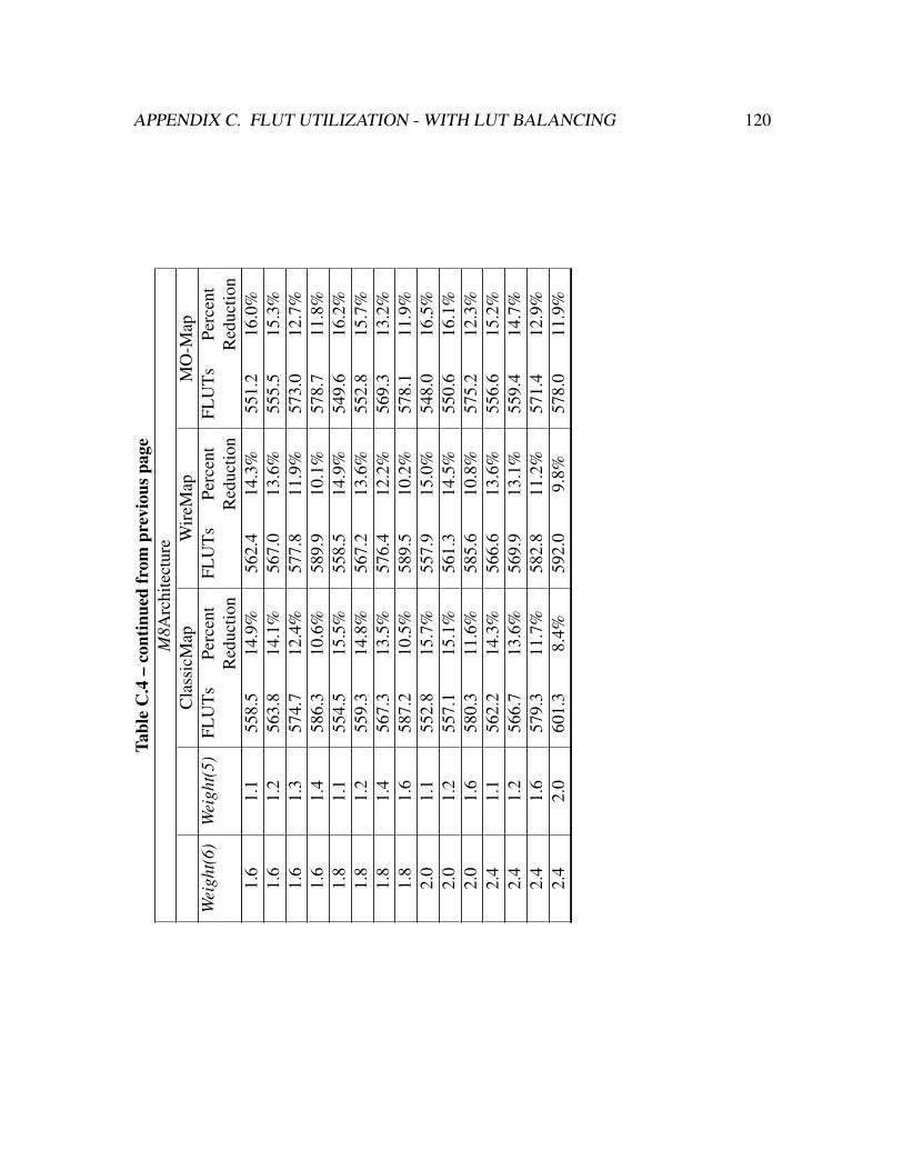
APPENDIX C. FLUT UTILIZATION - WITH LUT BALANCING 120Ta
ble
C.4
–co
ntin
ued
from
prev
ious
page
M8A
rchi
tect
ure
Cla
ssic
Map
Wir
eMap
MO
-Map
Wei
ght(
6)W
eigh
t(5)
FLU
Ts
Perc
ent
FLU
Ts
Perc
ent
FLU
Ts
Perc
ent
Red
uctio
nR
educ
tion
Red
uctio
n1.
61.
155
8.5
14.9
%56
2.4
14.3
%55
1.2
16.0
%1.
61.
256
3.8
14.1
%56
7.0
13.6
%55
5.5
15.3
%1.
61.
357
4.7
12.4
%57
7.8
11.9
%57
3.0
12.7
%1.
61.
458
6.3
10.6
%58
9.9
10.1
%57
8.7
11.8
%1.
81.
155
4.5
15.5
%55
8.5
14.9
%54
9.6
16.2
%1.
81.
255
9.3
14.8
%56
7.2
13.6
%55
2.8
15.7
%1.
81.
456
7.3
13.5
%57
6.4
12.2
%56
9.3
13.2
%1.
81.
658
7.2
10.5
%58
9.5
10.2
%57
8.1
11.9
%2.
01.
155
2.8
15.7
%55
7.9
15.0
%54
8.0
16.5
%2.
01.
255
7.1
15.1
%56
1.3
14.5
%55
0.6
16.1
%2.
01.
658
0.3
11.6
%58
5.6
10.8
%57
5.2
12.3
%2.
41.
156
2.2
14.3
%56
6.6
13.6
%55
6.6
15.2
%2.
41.
256
6.7
13.6
%56
9.9
13.1
%55
9.4
14.7
%2.
41.
657
9.3
11.7
%58
2.8
11.2
%57
1.4
12.9
%2.
42.
060
1.3
8.4%
592.
09.
8%57
8.0
11.9
%

APPENDIX C. FLUT UTILIZATION - WITH LUT BALANCING 121Ta
ble
C.5
:B
ench
mar
ksu
ite’s
FLU
Tut
iliza
tion
geom
etri
cm
ean
form
appi
ngs
prod
uced
with
LU
Tba
lanc
ing
and
pack
edfo
rthe
Stra
tixII
FPG
Aar
chite
ctur
e..E
ach
row
corr
espo
nds
toth
ese
tofm
appi
ngs
crea
ted
usin
gth
elis
ted
Wei
ght(
6)an
dW
eigh
t(5)
valu
es.F
LU
Tpe
rcen
tred
uctio
nis
calc
ulat
edw
ithre
spec
tto
the
arch
itect
ure’
sba
selin
em
appi
ng.
Stra
tixII
Arc
hite
ctur
eC
lass
icM
apW
ireM
apM
O-M
apW
eigh
t(6)
Wei
ght(
5)FL
UT
sPe
rcen
tFL
UT
sPe
rcen
tFL
UT
sPe
rcen
tR
educ
tion
Red
uctio
nR
educ
tion
1.0
1.0
651.
10.
0%60
2.3
7.5%
597.
38.
3%1.
11.
058
9.3
9.5%
589.
59.
5%57
7.6
11.3
%1.
21.
058
4.4
10.3
%58
6.2
10.0
%57
6.3
11.5
%1.
31.
058
4.4
10.3
%58
3.9
10.3
%57
6.0
11.5
%1.
41.
057
5.0
11.7
%57
8.0
11.2
%56
6.8
13.0
%1.
51.
057
3.8
11.9
%57
7.6
11.3
%56
7.8
12.8
%1.
61.
057
1.0
12.3
%57
1.0
12.3
%56
4.7
13.3
%1.
71.
057
3.8
11.9
%57
5.0
11.7
%56
2.9
13.5
%1.
81.
057
5.8
11.6
%57
3.7
11.9
%56
3.9
13.4
%1.
91.
057
5.3
11.6
%57
1.5
12.2
%56
4.4
13.3
%2.
01.
057
0.6
12.4
%57
2.6
12.1
%56
1.5
13.8
%2.
11.
058
7.4
9.8%
582.
010
.6%
576.
711
.4%
2.2
1.0
586.
69.
9%58
1.8
10.7
%57
5.1
11.7
%2.
31.
058
6.7
9.9%
582.
010
.6%
574.
711
.7%
2.4
1.0
586.
010
.0%
582.
210
.6%
575.
811
.6%
2.5
1.0
586.
59.
9%58
1.9
10.6
%57
5.4
11.6
%1.
21.
158
8.8
9.6%
591.
89.
1%58
6.4
9.9%
1.4
1.1
584.
910
.2%
585.
810
.0%
577.
311
.3%
1.4
1.2
589.
49.
5%58
9.7
9.4%
586.
59.
9%1.
41.
360
0.0
7.9%
600.
87.
7%59
5.5
8.5%
Con
tinue
don
next
page

APPENDIX C. FLUT UTILIZATION - WITH LUT BALANCING 122Ta
ble
C.5
–co
ntin
ued
from
prev
ious
page
Stra
tixII
Arc
hite
ctur
eC
lass
icM
apW
ireM
apM
O-M
apW
eigh
t(6)
Wei
ght(
5)FL
UT
sPe
rcen
tFL
UT
sPe
rcen
tFL
UT
sPe
rcen
tR
educ
tion
Red
uctio
nR
educ
tion
1.6
1.1
578.
511
.2%
582.
310
.6%
567.
412
.9%
1.6
1.2
582.
810
.5%
585.
210
.1%
569.
212
.6%
1.6
1.3
594.
78.
7%59
2.8
9.0%
587.
99.
7%1.
61.
460
2.4
7.5%
599.
97.
9%59
3.3
8.9%
1.8
1.1
572.
612
.1%
575.
911
.6%
566.
013
.1%
1.8
1.2
575.
511
.6%
586.
310
.0%
569.
012
.6%
1.8
1.4
584.
710
.2%
592.
29.
0%58
5.0
10.1
%1.
81.
660
1.9
7.6%
598.
68.
1%59
2.1
9.1%
2.0
1.1
574.
011
.9%
576.
211
.5%
567.
512
.8%
2.0
1.2
578.
311
.2%
578.
811
.1%
569.
312
.6%
2.0
1.6
594.
98.
6%59
8.8
8.0%
591.
09.
2%2.
41.
158
1.2
10.7
%58
6.1
10.0
%57
6.7
11.4
%2.
41.
258
5.4
10.1
%58
9.1
9.5%
579.
011
.1%
2.4
1.6
595.
98.
5%60
0.6
7.8%
587.
49.
8%2.
42.
061
8.1
5.1%
608.
36.
6%59
7.1
8.3%

Appendix D
VPR Minimum Channel Width
Geometric Means
123

APPENDIX D. VPR MINIMUM CHANNEL WIDTH GEOMETRIC MEANS 124Ta
ble
D.1
:B
ench
mar
ksu
ite’s
min
imum
min
imum
chan
nel
wid
thge
omet
ric
mea
nfo
rm
appi
ngs
prod
uced
with
LU
Tba
lanc
ing
and
pack
edfo
rthe
M5
FPG
Aar
chite
ctur
e..E
ach
row
corr
espo
nds
toth
ese
tofm
appi
ngs
crea
ted
usin
gth
elis
ted
Wei
ght(
6)an
dW
eigh
t(5)
valu
es.M
inim
umch
anne
lwid
thpe
rcen
tdiff
eren
ceis
calc
ulat
edw
ithre
spec
tto
the
arch
itect
ure’
sba
selin
em
appi
ng.
M5A
rchi
tect
ure
Cla
ssic
Map
Wir
eMap
MO
-Map
Wei
ght(
6)W
eigh
t(5)
MC
WPe
rcen
tM
CW
Perc
ent
MC
WPe
rcen
tD
iffer
ence
Diff
eren
ceD
iffer
ence
1.0
1.0
26.7
0.0%
28.1
5.1%
27.7
3.6%
1.1
1.0
27.4
2.4%
27.8
3.9%
27.5
2.9%
1.2
1.0
27.3
2.2%
27.6
3.2%
27.6
3.3%
1.3
1.0
27.2
1.9%
27.3
2.3%
27.7
3.7%
1.4
1.0
26.8
0.4%
27.5
2.8%
27.8
4.1%
1.5
1.0
27.0
1.1%
27.3
2.0%
27.7
3.6%
1.6
1.0
26.7
0.0%
27.2
1.7%
27.4
2.4%
1.7
1.0
27.2
1.7%
27.9
4.4%
27.9
4.5%
1.8
1.0
27.2
1.7%
27.6
3.3%
28.1
5.1%
1.9
1.0
26.9
0.7%
27.3
2.1%
27.9
4.5%
2.0
1.0
26.3
-1.4
%27
.32.
2%27
.73.
8%2.
11.
026
.4-1
.1%
27.2
1.9%
27.7
3.8%
2.2
1.0
26.3
-1.6
%26
.90.
8%27
.73.
7%2.
31.
026
.3-1
.6%
27.3
2.1%
27.7
3.6%
2.4
1.0
26.3
-1.4
%27
.11.
3%27
.84.
2%2.
51.
026
.3-1
.6%
27.5
2.8%
27.8
3.9%
1.2
1.1
27.6
3.1%
27.5
3.0%
27.5
3.0%
1.4
1.1
27.2
1.9%
27.7
3.7%
27.9
4.5%
1.4
1.2
27.4
2.5%
27.9
4.6%
28.0
4.7%
Con
tinue
don
next
page

APPENDIX D. VPR MINIMUM CHANNEL WIDTH GEOMETRIC MEANS 125Ta
ble
D.1
–co
ntin
ued
from
prev
ious
page
M5A
rchi
tect
ure
Cla
ssic
Map
Wir
eMap
MO
-Map
Wei
ght(
6)W
eigh
t(5)
MC
WPe
rcen
tM
CW
Perc
ent
MC
WPe
rcen
tD
iffer
ence
Diff
eren
ceD
iffer
ence
1.4
1.3
27.7
3.8%
28.1
5.1%
28.3
5.8%
1.6
1.1
27.1
1.3%
27.5
3.0%
27.9
4.6%
1.6
1.2
27.2
1.9%
27.6
3.4%
28.1
5.2%
1.6
1.3
27.7
3.7%
28.2
5.6%
28.3
5.7%
1.6
1.4
27.9
4.3%
28.5
6.8%
28.2
5.7%
1.8
1.1
26.8
0.3%
27.5
3.1%
27.8
4.0%
1.8
1.2
27.5
2.8%
27.8
4.0%
27.8
4.0%
1.8
1.4
27.1
1.3%
27.9
4.5%
28.0
4.9%
1.8
1.6
27.5
3.0%
28.2
5.5%
28.1
5.2%
2.0
1.1
26.6
-0.6
%27
.42.
7%27
.53.
1%2.
01.
226
.90.
6%27
.52.
8%27
.84.
0%2.
01.
627
.94.
4%27
.84.
2%28
.25.
7%2.
41.
126
.6-0
.3%
27.4
2.4%
27.6
3.2%
2.4
1.2
26.7
-0.2
%27
.73.
8%28
.15.
0%2.
41.
627
.32.
0%28
.15.
2%27
.94.
5%2.
42.
026
.90.
8%28
.15.
0%28
.35.
7%

APPENDIX D. VPR MINIMUM CHANNEL WIDTH GEOMETRIC MEANS 126Ta
ble
D.2
:B
ench
mar
ksu
ite’s
min
imum
chan
nelw
idth
geom
etri
cm
ean
form
appi
ngs
prod
uced
with
LU
Tba
lanc
ing
and
pack
edfo
rth
eM
6FP
GA
arch
itect
ure.
.E
ach
row
corr
espo
nds
toth
ese
tof
map
ping
scr
eate
dus
ing
the
liste
dW
eigh
t(6)
and
Wei
ght(
5)va
lues
.Min
imum
chan
nelw
idth
perc
entd
iffer
ence
isca
lcul
ated
with
resp
ectt
oth
ear
chite
ctur
e’s
base
line
map
ping
.
M6A
rchi
tect
ure
Cla
ssic
Map
Wir
eMap
MO
-Map
Wei
ght(
6)W
eigh
t(5)
MC
WPe
rcen
tM
CW
Perc
ent
MC
WPe
rcen
tD
iffer
ence
Diff
eren
ceD
iffer
ence
1.0
1.0
29.5
0.0%
30.8
4.5%
31.0
5.3%
1.1
1.0
30.1
2.3%
31.3
6.3%
31.4
6.4%
1.2
1.0
29.9
1.6%
31.4
6.6%
31.4
6.7%
1.3
1.0
30.2
2.3%
31.4
6.6%
31.8
7.8%
1.4
1.0
30.2
2.3%
31.6
7.3%
31.6
7.1%
1.5
1.0
29.9
1.6%
31.6
7.1%
31.8
8.0%
1.6
1.0
29.9
1.4%
31.4
6.5%
31.7
7.6%
1.7
1.0
30.1
2.3%
31.7
7.6%
31.6
7.4%
1.8
1.0
30.1
2.1%
31.4
6.4%
31.6
7.2%
1.9
1.0
29.7
0.8%
31.0
5.2%
31.5
7.0%
2.0
1.0
29.7
0.9%
31.2
5.9%
31.7
7.4%
2.1
1.0
30.3
2.7%
32.5
10.4
%33
.112
.4%
2.2
1.0
29.9
1.5%
32.3
9.6%
33.0
12.0
%2.
31.
029
.70.
9%32
.29.
4%33
.011
.9%
2.4
1.0
29.9
1.6%
32.5
10.3
%32
.811
.2%
2.5
1.0
29.8
1.2%
32.9
11.6
%32
.811
.2%
1.2
1.1
30.8
4.6%
31.1
5.5%
31.7
7.6%
1.4
1.1
31.4
6.5%
31.8
7.8%
32.1
9.1%
1.4
1.3
31.1
5.6%
31.6
7.2%
31.9
8.1%
Con
tinue
don
next
page

APPENDIX D. VPR MINIMUM CHANNEL WIDTH GEOMETRIC MEANS 127Ta
ble
D.2
–co
ntin
ued
from
prev
ious
page
M6A
rchi
tect
ure
Cla
ssic
Map
Wir
eMap
MO
-Map
Wei
ght(
6)W
eigh
t(5)
MC
WPe
rcen
tM
CW
Perc
ent
MC
WPe
rcen
tD
iffer
ence
Diff
eren
ceD
iffer
ence
1.4
1.4
31.2
5.9%
32.0
8.7%
32.0
8.4%
1.6
1.1
30.9
4.7%
31.3
6.1%
32.1
9.0%
1.6
1.2
30.6
4.0%
31.7
7.7%
32.2
9.3%
1.6
1.3
31.1
5.7%
32.1
8.8%
32.7
10.9
%1.
61.
431
.36.
4%31
.77.
7%32
.39.
5%1.
81.
131
.15.
6%31
.98.
1%32
.410
.0%
1.8
1.2
31.0
5.3%
31.5
7.0%
31.9
8.3%
1.8
1.4
31.3
6.2%
32.0
8.6%
32.3
9.6%
1.8
1.6
32.0
8.4%
32.4
9.8%
32.0
8.7%
2.0
1.1
31.0
5.1%
31.5
6.9%
31.9
8.2%
2.0
1.2
31.4
6.6%
32.0
8.5%
32.2
9.2%
2.0
1.6
31.4
6.5%
32.0
8.6%
32.4
10.0
%2.
41.
131
.87.
9%32
.510
.3%
33.3
13.1
%2.
41.
232
.08.
7%32
.911
.7%
33.5
13.6
%2.
41.
632
.29.
1%33
.112
.2%
33.1
12.3
%2.
42.
032
.19.
1%33
.212
.6%
33.3
12.8
%

APPENDIX D. VPR MINIMUM CHANNEL WIDTH GEOMETRIC MEANS 128Ta
ble
D.3
:B
ench
mar
ksu
ite’s
min
imum
chan
nelw
idth
geom
etri
cm
ean
form
appi
ngs
prod
uced
with
LU
Tba
lanc
ing
and
pack
edfo
rth
eM
7FP
GA
arch
itect
ure.
.E
ach
row
corr
espo
nds
toth
ese
tof
map
ping
scr
eate
dus
ing
the
liste
dW
eigh
t(6)
and
Wei
ght(
5)va
lues
.Min
imum
chan
nelw
idth
perc
entd
iffer
ence
isca
lcul
ated
with
resp
ectt
oth
ear
chite
ctur
e’s
base
line
map
ping
.
M7A
rchi
tect
ure
Cla
ssic
Map
Wir
eMap
MO
-Map
Wei
ght(
6)W
eigh
t(5)
MC
WPe
rcen
tM
CW
Perc
ent
MC
WPe
rcen
tD
iffer
ence
Diff
eren
ceD
iffer
ence
1.0
1.0
31.3
0.0%
31.9
2.1%
33.1
6.0%
1.1
1.0
32.6
4.1%
33.2
6.1%
33.6
7.4%
1.2
1.0
33.0
5.7%
33.3
6.6%
34.0
8.7%
1.3
1.0
33.1
5.7%
33.3
6.4%
34.3
9.6%
1.4
1.0
33.5
7.2%
33.8
8.0%
34.1
9.2%
1.5
1.0
33.4
6.8%
33.9
8.3%
34.2
9.4%
1.6
1.0
33.5
7.0%
34.0
8.6%
34.6
10.6
%1.
71.
033
.67.
4%33
.98.
3%34
.610
.5%
1.8
1.0
33.5
7.0%
33.8
8.2%
34.5
10.2
%1.
91.
033
.67.
3%33
.67.
6%34
.410
.1%
2.0
1.0
33.2
6.2%
34.2
9.4%
35.0
11.8
%2.
11.
033
.57.
3%34
.911
.6%
35.9
14.8
%2.
21.
033
.77.
8%34
.911
.6%
35.9
14.7
%2.
31.
033
.77.
6%34
.911
.5%
35.7
14.1
%2.
41.
033
.67.
4%34
.911
.4%
36.1
15.5
%2.
51.
033
.77.
6%34
.811
.2%
36.1
15.5
%1.
21.
133
.05.
5%33
.26.
1%33
.67.
4%1.
41.
133
.46.
8%34
.510
.2%
33.4
6.8%
1.4
1.2
33.1
5.8%
33.9
8.4%
32.9
5.3%
Con
tinue
don
next
page

APPENDIX D. VPR MINIMUM CHANNEL WIDTH GEOMETRIC MEANS 129Ta
ble
D.3
–co
ntin
ued
from
prev
ious
page
M7A
rchi
tect
ure
Cla
ssic
Map
Wir
eMap
MO
-Map
Wei
ght(
6)W
eigh
t(5)
MC
WPe
rcen
tM
CW
Perc
ent
MC
WPe
rcen
tD
iffer
ence
Diff
eren
ceD
iffer
ence
1.4
1.3
33.0
5.5%
33.7
7.7%
33.1
5.8%
1.6
1.1
33.1
5.8%
33.3
6.4%
34.4
10.1
%1.
61.
233
.26.
1%33
.57.
3%34
.39.
5%1.
61.
333
.46.
8%33
.26.
1%33
.77.
8%1.
61.
433
.15.
8%32
.53.
8%33
.98.
4%1.
81.
133
.87.
9%33
.46.
9%34
.29.
3%1.
81.
233
.98.
5%33
.88.
2%34
.811
.4%
1.8
1.4
33.7
7.7%
33.5
7.1%
34.2
9.5%
1.8
1.6
33.3
6.4%
33.1
6.0%
34.0
8.8%
2.0
1.1
33.7
7.6%
33.6
7.3%
34.6
10.7
%2.
01.
233
.57.
2%33
.77.
7%34
.610
.5%
2.0
1.6
33.7
7.8%
33.2
6.2%
34.1
9.0%
2.4
1.1
34.7
10.9
%34
.811
.1%
35.7
14.3
%2.
41.
235
.012
.0%
35.3
12.8
%35
.413
.3%
2.4
1.6
34.6
10.6
%34
.19.
0%34
.711
.1%
2.4
2.0
34.7
10.9
%34
.08.
8%34
.510
.3%

APPENDIX D. VPR MINIMUM CHANNEL WIDTH GEOMETRIC MEANS 130Ta
ble
D.4
:B
ench
mar
ksu
ite’s
min
imum
chan
nelw
idth
geom
etri
cm
ean
form
appi
ngs
prod
uced
with
LU
Tba
lanc
ing
and
pack
edfo
rth
eM
8FP
GA
arch
itect
ure.
.E
ach
row
corr
espo
nds
toth
ese
tof
map
ping
scr
eate
dus
ing
the
liste
dW
eigh
t(6)
and
Wei
ght(
5)va
lues
.Min
imum
chan
nelw
idth
perc
entd
iffer
ence
isca
lcul
ated
with
resp
ectt
oth
ear
chite
ctur
e’s
base
line
map
ping
.
M8A
rchi
tect
ure
Cla
ssic
Map
Wir
eMap
MO
-Map
Wei
ght(
6)W
eigh
t(5)
MC
WPe
rcen
tM
CW
Perc
ent
MC
WPe
rcen
tD
iffer
ence
Diff
eren
ceD
iffer
ence
1.0
1.0
31.8
0.0%
32.8
3.3%
33.7
6.0%
1.1
1.0
33.9
6.8%
33.5
5.5%
34.2
7.7%
1.2
1.0
34.6
9.0%
33.4
5.1%
34.0
6.9%
1.3
1.0
34.5
8.6%
34.0
7.0%
34.1
7.2%
1.4
1.0
35.0
10.3
%34
.37.
9%34
.79.
3%1.
51.
034
.99.
9%34
.07.
0%34
.89.
7%1.
61.
035
.010
.1%
34.1
7.3%
34.5
8.7%
1.7
1.0
35.0
10.1
%34
.58.
5%34
.99.
9%1.
81.
035
.110
.6%
34.7
9.2%
35.0
10.1
%1.
91.
035
.110
.6%
34.4
8.2%
34.8
9.5%
2.0
1.0
35.4
11.4
%34
.79.
3%35
.110
.5%
2.1
1.0
35.9
13.0
%35
.612
.1%
36.3
14.3
%2.
21.
036
.414
.5%
35.6
12.0
%36
.314
.2%
2.3
1.0
36.1
13.6
%35
.411
.5%
36.7
15.5
%2.
41.
036
.013
.3%
35.6
12.1
%36
.615
.3%
2.5
1.0
36.2
13.9
%35
.712
.5%
36.7
15.6
%1.
21.
133
.76.
0%33
.45.
2%33
.96.
6%1.
41.
134
.38.
1%33
.96.
7%34
.37.
9%1.
41.
233
.86.
5%33
.55.
3%34
.38.
0%C
ontin
ued
onne
xtpa
ge

APPENDIX D. VPR MINIMUM CHANNEL WIDTH GEOMETRIC MEANS 131Ta
ble
D.4
–co
ntin
ued
from
prev
ious
page
M8A
rchi
tect
ure
Cla
ssic
Map
Wir
eMap
MO
-Map
Wei
ght(
6)W
eigh
t(5)
MC
WPe
rcen
tM
CW
Perc
ent
MC
WPe
rcen
tD
iffer
ence
Diff
eren
ceD
iffer
ence
1.4
1.3
33.6
5.9%
33.4
5.3%
33.9
6.7%
1.6
1.1
34.7
9.1%
34.1
7.3%
34.6
8.9%
1.6
1.2
34.5
8.5%
34.3
7.8%
34.8
9.5%
1.6
1.3
34.3
7.8%
33.7
6.0%
34.1
7.3%
1.6
1.4
33.7
6.1%
32.8
3.3%
33.9
6.9%
1.8
1.1
35.1
10.5
%34
.58.
5%35
.110
.6%
1.8
1.2
34.8
9.6%
34.3
8.1%
34.6
8.8%
1.8
1.4
34.7
9.2%
33.7
6.1%
34.8
9.5%
1.8
1.6
34.0
7.2%
33.2
4.5%
34.1
7.4%
2.0
1.1
35.2
10.9
%34
.48.
4%34
.68.
9%2.
01.
234
.89.
6%34
.27.
6%34
.79.
3%2.
01.
635
.210
.8%
34.0
7.1%
34.5
8.8%
2.4
1.1
36.4
14.7
%35
.812
.6%
36.4
14.5
%2.
41.
236
.214
.1%
36.0
13.3
%36
.414
.7%
2.4
1.6
36.1
13.6
%35
.411
.3%
35.6
12.1
%2.
42.
035
.210
.8%
35.0
10.3
%34
.69.
1%

Appendix E
VPR Wirelength Geometric Means
132

APPENDIX E. VPR WIRELENGTH GEOMETRIC MEANS 133Ta
ble
E.1
:Ben
chm
ark
suite
’sw
irel
engt
hge
omet
ric
mea
nfo
rmap
ping
spr
oduc
edw
ithL
UT
bala
ncin
gan
dpa
cked
fort
heM
5FP
GA
arch
itect
ure.
.E
ach
row
corr
espo
nds
toth
ese
tof
map
ping
scr
eate
dus
ing
the
liste
dW
eigh
t(6)
and
Wei
ght(
5)va
lues
.Wir
elen
gth
perc
entd
iffer
ence
isca
lcul
ated
with
resp
ectt
oth
ear
chite
ctur
e’s
base
line
map
ping
.
M5A
rchi
tect
ure
Cla
ssic
Map
Wir
eMap
MO
-Map
Wei
ght(
6)W
eigh
t(5)
Wir
elen
gth
Perc
ent
Wir
elen
gth
Perc
ent
Wir
elen
gth
Perc
ent
Diff
eren
ceD
iffer
ence
Diff
eren
ce1.
01.
026
.70.
0%28
.15.
1%27
.73.
6%1.
11.
027
.42.
4%27
.83.
9%27
.52.
9%1.
21.
027
.32.
2%27
.63.
2%27
.63.
3%1.
31.
027
.21.
9%27
.32.
3%27
.73.
7%1.
41.
026
.80.
4%27
.52.
8%27
.84.
1%1.
51.
027
.01.
1%27
.32.
0%27
.73.
6%1.
61.
026
.70.
0%27
.21.
7%27
.42.
4%1.
71.
027
.21.
7%27
.94.
4%27
.94.
5%1.
81.
027
.21.
7%27
.63.
3%28
.15.
1%1.
91.
026
.90.
7%27
.32.
1%27
.94.
5%2.
01.
026
.3-1
.4%
27.3
2.2%
27.7
3.8%
2.1
1.0
26.4
-1.1
%27
.21.
9%27
.73.
8%2.
21.
026
.3-1
.6%
26.9
0.8%
27.7
3.7%
2.3
1.0
26.3
-1.6
%27
.32.
1%27
.73.
6%2.
41.
026
.3-1
.4%
27.1
1.3%
27.8
4.2%
2.5
1.0
26.3
-1.6
%27
.52.
8%27
.83.
9%1.
21.
127
.63.
1%27
.53.
0%27
.53.
0%1.
41.
127
.21.
9%27
.73.
7%27
.94.
5%1.
41.
227
.42.
5%27
.94.
6%28
.04.
7%1.
41.
327
.73.
8%28
.15.
1%28
.35.
8%C
ontin
ued
onne
xtpa
ge

APPENDIX E. VPR WIRELENGTH GEOMETRIC MEANS 134Ta
ble
E.1
–co
ntin
ued
from
prev
ious
page
M5A
rchi
tect
ure
Cla
ssic
Map
Wir
eMap
MO
-Map
Wei
ght(
6)W
eigh
t(5)
Wir
elen
gth
Perc
ent
Wir
elen
gth
Perc
ent
Wir
elen
gth
Perc
ent
Diff
eren
ceD
iffer
ence
Diff
eren
ce1.
61.
127
.11.
3%27
.53.
0%27
.94.
6%1.
61.
227
.21.
9%27
.63.
4%28
.15.
2%1.
61.
327
.73.
7%28
.25.
6%28
.35.
7%1.
61.
427
.94.
3%28
.56.
8%28
.25.
7%1.
81.
126
.80.
3%27
.53.
1%27
.84.
0%1.
81.
227
.52.
8%27
.84.
0%27
.84.
0%1.
81.
427
.11.
3%27
.94.
5%28
.04.
9%1.
81.
627
.53.
0%28
.25.
5%28
.15.
2%2.
01.
126
.6-0
.6%
27.4
2.7%
27.5
3.1%
2.0
1.2
26.9
0.6%
27.5
2.8%
27.8
4.0%
2.0
1.6
27.9
4.4%
27.8
4.2%
28.2
5.7%
2.4
1.1
26.6
-0.3
%27
.42.
4%27
.63.
2%2.
41.
226
.7-0
.2%
27.7
3.8%
28.1
5.0%
2.4
1.6
27.3
2.0%
28.1
5.2%
27.9
4.5%
2.4
2.0
26.9
0.8%
28.1
5.0%
28.3
5.7%

APPENDIX E. VPR WIRELENGTH GEOMETRIC MEANS 135Ta
ble
E.2
:B
ench
mar
ksu
ite’s
wir
elen
gth
wid
thge
omet
ric
mea
nfo
rmap
ping
spr
oduc
edw
ithL
UT
bala
ncin
gan
dpa
cked
for
the
M6
FPG
Aar
chite
ctur
e..
Eac
hro
wco
rres
pond
sto
the
set
ofm
appi
ngs
crea
ted
usin
gth
elis
ted
Wei
ght(
6)an
dW
eigh
t(5)
valu
es.W
irel
engt
hpe
rcen
tdiff
eren
ceis
calc
ulat
edw
ithre
spec
tto
the
arch
itect
ure’
sba
selin
em
appi
ng.
M6A
rchi
tect
ure
Cla
ssic
Map
Wir
eMap
MO
-Map
Wei
ght(
6)W
eigh
t(5)
Wir
elen
gth
Perc
ent
Wir
elen
gth
Perc
ent
Wir
elen
gth
Perc
ent
Diff
eren
ceD
iffer
ence
Diff
eren
ce1.
01.
029
.50.
0%30
.84.
5%31
.05.
3%1.
11.
030
.12.
3%31
.36.
3%31
.46.
4%1.
21.
029
.91.
6%31
.46.
6%31
.46.
7%1.
31.
030
.22.
3%31
.46.
6%31
.87.
8%1.
41.
030
.22.
3%31
.67.
3%31
.67.
1%1.
51.
029
.91.
6%31
.67.
1%31
.88.
0%1.
61.
029
.91.
4%31
.46.
5%31
.77.
6%1.
71.
030
.12.
3%31
.77.
6%31
.67.
4%1.
81.
030
.12.
1%31
.46.
4%31
.67.
2%1.
91.
029
.70.
8%31
.05.
2%31
.57.
0%2.
01.
029
.70.
9%31
.25.
9%31
.77.
4%2.
11.
030
.32.
7%32
.510
.4%
33.1
12.4
%2.
21.
029
.91.
5%32
.39.
6%33
.012
.0%
2.3
1.0
29.7
0.9%
32.2
9.4%
33.0
11.9
%2.
41.
029
.91.
6%32
.510
.3%
32.8
11.2
%2.
51.
029
.81.
2%32
.911
.6%
32.8
11.2
%1.
21.
130
.84.
6%31
.15.
5%31
.77.
6%1.
41.
131
.46.
5%31
.87.
8%32
.19.
1%1.
41.
331
.15.
6%31
.67.
2%31
.98.
1%1.
41.
431
.25.
9%32
.08.
7%32
.08.
4%C
ontin
ued
onne
xtpa
ge

APPENDIX E. VPR WIRELENGTH GEOMETRIC MEANS 136Ta
ble
E.2
–co
ntin
ued
from
prev
ious
page
M6A
rchi
tect
ure
Cla
ssic
Map
Wir
eMap
MO
-Map
Wei
ght(
6)W
eigh
t(5)
Wir
elen
gth
Perc
ent
Wir
elen
gth
Perc
ent
Wir
elen
gth
Perc
ent
Diff
eren
ceD
iffer
ence
Diff
eren
ce1.
61.
130
.94.
7%31
.36.
1%32
.19.
0%1.
61.
230
.64.
0%31
.77.
7%32
.29.
3%1.
61.
331
.15.
7%32
.18.
8%32
.710
.9%
1.6
1.4
31.3
6.4%
31.7
7.7%
32.3
9.5%
1.8
1.1
31.1
5.6%
31.9
8.1%
32.4
10.0
%1.
81.
231
.05.
3%31
.57.
0%31
.98.
3%1.
81.
431
.36.
2%32
.08.
6%32
.39.
6%1.
81.
632
.08.
4%32
.49.
8%32
.08.
7%2.
01.
131
.05.
1%31
.56.
9%31
.98.
2%2.
01.
231
.46.
6%32
.08.
5%32
.29.
2%2.
01.
631
.46.
5%32
.08.
6%32
.410
.0%
2.4
1.1
31.8
7.9%
32.5
10.3
%33
.313
.1%
2.4
1.2
32.0
8.7%
32.9
11.7
%33
.513
.6%
2.4
1.6
32.2
9.1%
33.1
12.2
%33
.112
.3%
2.4
2.0
32.1
9.1%
33.2
12.6
%33
.312
.8%

APPENDIX E. VPR WIRELENGTH GEOMETRIC MEANS 137Ta
ble
E.3
:Ben
chm
ark
suite
’sw
irel
engt
hge
omet
ric
mea
nfo
rmap
ping
spr
oduc
edw
ithL
UT
bala
ncin
gan
dpa
cked
fort
heM
7FP
GA
arch
itect
ure.
.E
ach
row
corr
espo
nds
toth
ese
tof
map
ping
scr
eate
dus
ing
the
liste
dW
eigh
t(6)
and
Wei
ght(
5)va
lues
.Wir
elen
gth
perc
entd
iffer
ence
isca
lcul
ated
with
resp
ectt
oth
ear
chite
ctur
e’s
base
line
map
ping
.
M7A
rchi
tect
ure
Cla
ssic
Map
Wir
eMap
MO
-Map
Wei
ght(
6)W
eigh
t(5)
Wir
elen
gth
Perc
ent
Wir
elen
gth
Perc
ent
Wir
elen
gth
Perc
ent
Diff
eren
ceD
iffer
ence
Diff
eren
ce1.
01.
031
.30.
0%31
.92.
1%33
.16.
0%1.
11.
032
.64.
1%33
.26.
1%33
.67.
4%1.
21.
033
.05.
7%33
.36.
6%34
.08.
7%1.
31.
033
.15.
7%33
.36.
4%34
.39.
6%1.
41.
033
.57.
2%33
.88.
0%34
.19.
2%1.
51.
033
.46.
8%33
.98.
3%34
.29.
4%1.
61.
033
.57.
0%34
.08.
6%34
.610
.6%
1.7
1.0
33.6
7.4%
33.9
8.3%
34.6
10.5
%1.
81.
033
.57.
0%33
.88.
2%34
.510
.2%
1.9
1.0
33.6
7.3%
33.6
7.6%
34.4
10.1
%2.
01.
033
.26.
2%34
.29.
4%35
.011
.8%
2.1
1.0
33.5
7.3%
34.9
11.6
%35
.914
.8%
2.2
1.0
33.7
7.8%
34.9
11.6
%35
.914
.7%
2.3
1.0
33.7
7.6%
34.9
11.5
%35
.714
.1%
2.4
1.0
33.6
7.4%
34.9
11.4
%36
.115
.5%
2.5
1.0
33.7
7.6%
34.8
11.2
%36
.115
.5%
1.2
1.1
33.0
5.5%
33.2
6.1%
33.6
7.4%
1.4
1.1
33.4
6.8%
34.5
10.2
%33
.46.
8%1.
41.
233
.15.
8%33
.98.
4%32
.95.
3%1.
41.
333
.05.
5%33
.77.
7%33
.15.
8%C
ontin
ued
onne
xtpa
ge

APPENDIX E. VPR WIRELENGTH GEOMETRIC MEANS 138Ta
ble
E.3
–co
ntin
ued
from
prev
ious
page
M7A
rchi
tect
ure
Cla
ssic
Map
Wir
eMap
MO
-Map
Wei
ght(
6)W
eigh
t(5)
Wir
elen
gth
Perc
ent
Wir
elen
gth
Perc
ent
Wir
elen
gth
Perc
ent
Diff
eren
ceD
iffer
ence
Diff
eren
ce1.
61.
133
.15.
8%33
.36.
4%34
.410
.1%
1.6
1.2
33.2
6.1%
33.5
7.3%
34.3
9.5%
1.6
1.3
33.4
6.8%
33.2
6.1%
33.7
7.8%
1.6
1.4
33.1
5.8%
32.5
3.8%
33.9
8.4%
1.8
1.1
33.8
7.9%
33.4
6.9%
34.2
9.3%
1.8
1.2
33.9
8.5%
33.8
8.2%
34.8
11.4
%1.
81.
433
.77.
7%33
.57.
1%34
.29.
5%1.
81.
633
.36.
4%33
.16.
0%34
.08.
8%2.
01.
133
.77.
6%33
.67.
3%34
.610
.7%
2.0
1.2
33.5
7.2%
33.7
7.7%
34.6
10.5
%2.
01.
633
.77.
8%33
.26.
2%34
.19.
0%2.
41.
134
.710
.9%
34.8
11.1
%35
.714
.3%
2.4
1.2
35.0
12.0
%35
.312
.8%
35.4
13.3
%2.
41.
634
.610
.6%
34.1
9.0%
34.7
11.1
%2.
42.
034
.710
.9%
34.0
8.8%
34.5
10.3
%

APPENDIX E. VPR WIRELENGTH GEOMETRIC MEANS 139Ta
ble
E.4
:Ben
chm
ark
suite
’sw
irel
engt
hge
omet
ric
mea
nfo
rmap
ping
spr
oduc
edw
ithL
UT
bala
ncin
gan
dpa
cked
fort
heM
8FP
GA
arch
itect
ure.
.E
ach
row
corr
espo
nds
toth
ese
tof
map
ping
scr
eate
dus
ing
the
liste
dW
eigh
t(6)
and
Wei
ght(
5)va
lues
.Wir
elen
gth
perc
entd
iffer
ence
isca
lcul
ated
with
resp
ectt
oth
ear
chite
ctur
e’s
base
line
map
ping
.
M8A
rchi
tect
ure
Cla
ssic
Map
Wir
eMap
MO
-Map
Wei
ght(
6)W
eigh
t(5)
Wir
elen
gth
Perc
ent
Wir
elen
gth
Perc
ent
Wir
elen
gth
Perc
ent
Diff
eren
ceD
iffer
ence
Diff
eren
ce1.
01.
031
.80.
0%32
.83.
3%33
.76.
0%1.
11.
033
.96.
8%33
.55.
5%34
.27.
7%1.
21.
034
.69.
0%33
.45.
1%34
.06.
9%1.
31.
034
.58.
6%34
.07.
0%34
.17.
2%1.
41.
035
.010
.3%
34.3
7.9%
34.7
9.3%
1.5
1.0
34.9
9.9%
34.0
7.0%
34.8
9.7%
1.6
1.0
35.0
10.1
%34
.17.
3%34
.58.
7%1.
71.
035
.010
.1%
34.5
8.5%
34.9
9.9%
1.8
1.0
35.1
10.6
%34
.79.
2%35
.010
.1%
1.9
1.0
35.1
10.6
%34
.48.
2%34
.89.
5%2.
01.
035
.411
.4%
34.7
9.3%
35.1
10.5
%2.
11.
035
.913
.0%
35.6
12.1
%36
.314
.3%
2.2
1.0
36.4
14.5
%35
.612
.0%
36.3
14.2
%2.
31.
036
.113
.6%
35.4
11.5
%36
.715
.5%
2.4
1.0
36.0
13.3
%35
.612
.1%
36.6
15.3
%2.
51.
036
.213
.9%
35.7
12.5
%36
.715
.6%
1.2
1.1
33.7
6.0%
33.4
5.2%
33.9
6.6%
1.4
1.1
34.3
8.1%
33.9
6.7%
34.3
7.9%
1.4
1.2
33.8
6.5%
33.5
5.3%
34.3
8.0%
1.4
1.3
33.6
5.9%
33.4
5.3%
33.9
6.7%
Con
tinue
don
next
page

APPENDIX E. VPR WIRELENGTH GEOMETRIC MEANS 140Ta
ble
E.4
–co
ntin
ued
from
prev
ious
page
M8A
rchi
tect
ure
Cla
ssic
Map
Wir
eMap
MO
-Map
Wei
ght(
6)W
eigh
t(5)
Wir
elen
gth
Perc
ent
Wir
elen
gth
Perc
ent
Wir
elen
gth
Perc
ent
Diff
eren
ceD
iffer
ence
Diff
eren
ce1.
61.
134
.79.
1%34
.17.
3%34
.68.
9%1.
61.
234
.58.
5%34
.37.
8%34
.89.
5%1.
61.
334
.37.
8%33
.76.
0%34
.17.
3%1.
61.
433
.76.
1%32
.83.
3%33
.96.
9%1.
81.
135
.110
.5%
34.5
8.5%
35.1
10.6
%1.
81.
234
.89.
6%34
.38.
1%34
.68.
8%1.
81.
434
.79.
2%33
.76.
1%34
.89.
5%1.
81.
634
.07.
2%33
.24.
5%34
.17.
4%2.
01.
135
.210
.9%
34.4
8.4%
34.6
8.9%
2.0
1.2
34.8
9.6%
34.2
7.6%
34.7
9.3%
2.0
1.6
35.2
10.8
%34
.07.
1%34
.58.
8%2.
41.
136
.414
.7%
35.8
12.6
%36
.414
.5%
2.4
1.2
36.2
14.1
%36
.013
.3%
36.4
14.7
%2.
41.
636
.113
.6%
35.4
11.3
%35
.612
.1%
2.4
2.0
35.2
10.8
%35
.010
.3%
34.6
9.1%

Appendix F
Quartus II Fmax Geometric Means
141

APPENDIX F. QUARTUS II FMAX GEOMETRIC MEANS 142Ta
ble
F.1:
Ben
chm
ark
suite
’sm
axim
umop
erat
ing
freq
uenc
y(F
max
)ge
omet
ric
mea
nfo
rm
appi
ngs
prod
uced
with
LU
Tba
lanc
ing
and
pack
edfo
rth
eSt
ratix
IIFP
GA
arch
itect
ure.
.E
ach
row
corr
espo
nds
toth
ese
tof
map
ping
scr
eate
dus
ing
the
liste
dW
eigh
t(6)
and
Wei
ght(
5)va
lues
.Max
imum
oper
atin
gfr
eque
ncy
perc
entd
iffer
ence
isca
lcul
ated
with
resp
ectt
oth
ear
chite
ctur
e’s
base
line
map
ping
.
Stra
tixII
Arc
hite
ctur
eC
lass
icM
apW
ireM
apM
O-M
apW
eigh
t(6)
Wei
ght(
5)Fm
ax(M
Hz)
Perc
ent
Fmax
(MH
z)Pe
rcen
tFm
ax(M
Hz)
Perc
ent
Diff
eren
ceD
iffer
ence
Diff
eren
ce1.
01.
019
3.9
0.0%
193.
1-0
.4%
193.
7-0
.1%
1.1
1.0
192.
8-0
.6%
193.
4-0
.3%
195.
91.
0%1.
21.
019
2.2
-0.9
%19
3.2
-0.3
%19
3.9
0.0%
1.3
1.0
192.
2-0
.9%
192.
3-0
.8%
192.
4-0
.8%
1.4
1.0
192.
6-0
.7%
193.
6-0
.2%
193.
6-0
.2%
1.5
1.0
192.
8-0
.5%
193.
6-0
.2%
192.
4-0
.8%
1.6
1.0
193.
0-0
.5%
194.
20.
1%19
2.8
-0.6
%1.
71.
019
3.7
-0.1
%19
5.6
0.9%
192.
9-0
.5%
1.8
1.0
192.
7-0
.6%
193.
7-0
.1%
195.
10.
6%1.
91.
019
2.0
-1.0
%19
3.2
-0.4
%19
4.8
0.4%
2.0
1.0
191.
8-1
.1%
194.
80.
5%19
3.4
-0.3
%2.
11.
019
3.6
-0.2
%19
2.6
-0.7
%19
0.3
-1.9
%2.
21.
019
2.4
-0.8
%19
4.4
0.2%
193.
1-0
.4%
2.3
1.0
191.
4-1
.3%
192.
2-0
.9%
192.
7-0
.6%
2.4
1.0
191.
7-1
.1%
192.
6-0
.7%
192.
0-1
.0%
2.5
1.0
191.
9-1
.0%
192.
6-0
.7%
191.
8-1
.1%
1.2
1.1
195.
00.
6%19
4.2
0.1%
193.
8-0
.1%
1.4
1.1
193.
2-0
.3%
192.
9-0
.5%
194.
40.
2%1.
41.
219
3.4
-0.3
%19
2.2
-0.9
%19
4.3
0.2%
Con
tinue
don
next
page
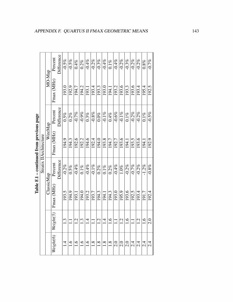
APPENDIX F. QUARTUS II FMAX GEOMETRIC MEANS 143Ta
ble
F.1
–co
ntin
ued
from
prev
ious
page
Stra
tixII
Arc
hite
ctur
eC
lass
icM
apW
ireM
apM
O-M
apW
eigh
t(6)
Wei
ght(
5)Fm
ax(M
Hz)
Perc
ent
Fmax
(MH
z)Pe
rcen
tFm
ax(M
Hz)
Perc
ent
Diff
eren
ceD
iffer
ence
Diff
eren
ce1.
41.
319
3.5
-0.2
%19
4.9
0.5%
193.
0-0
.5%
1.6
1.1
194.
90.
5%19
4.3
0.2%
192.
9-0
.5%
1.6
1.2
193.
1-0
.4%
192.
6-0
.7%
194.
70.
4%1.
61.
319
4.0
0.1%
192.
2-0
.9%
194.
20.
2%1.
61.
419
3.2
-0.4
%19
4.6
0.3%
193.
1-0
.4%
1.8
1.1
193.
7-0
.1%
192.
4-0
.8%
193.
4-0
.2%
1.8
1.2
194.
30.
2%19
4.0
0.0%
193.
3-0
.3%
1.8
1.4
194.
10.
1%19
3.8
-0.1
%19
3.0
-0.4
%1.
81.
619
4.3
0.2%
194.
70.
4%19
4.1
0.1%
2.0
1.1
193.
0-0
.4%
192.
7-0
.6%
193.
2-0
.4%
2.0
1.2
195.
91.
0%19
3.6
-0.1
%19
3.6
-0.2
%2.
01.
619
3.6
-0.2
%19
4.1
0.1%
193.
3-0
.3%
2.4
1.1
192.
5-0
.7%
193.
5-0
.2%
193.
6-0
.2%
2.4
1.2
193.
4-0
.2%
193.
6-0
.2%
193.
4-0
.2%
2.4
1.6
191.
7-1
.2%
194.
10.
1%19
5.4
0.8%
2.4
2.0
192.
4-0
.8%
192.
9-0
.5%
192.
5-0
.7%