FPGA Implementation of - Computer Engineering …pc/research/publications/lee... · Web...

An FPGA Implementation of the Smooth Particle Mesh Ewald

Reciprocal Sum Compute Engine (RSCE)

bBy

Sam Lee

A thesis submitted in partial conformity withfulfillment of the requirements for the

degree of Master of Applied Science Master of Applied Science

Graduate Department of Electrical and Computer Engineering of University of Toronto

1

© Copyright by Sam Lee 2005

2

An FPGA Implementation of theSmooth Particle Mesh Ewald

Reciprocal Sum Compute Engine (RSCE)

Sam Lee

Master of Applied Science, 2005

Chairperson of the Supervisory Committee:Professor Paul Chow

Graduate Department of Electrical and Computer EngineeringUniversity of Toronto

AbstractAbstract

Currently, Mmolecular dynamics simulations are mostly carried outaccelerated by supercomputers that are made up of either by a clusters of microprocessors or by a custom ASIC systems. However, Tthe power dissipation of the microprocessors and the non-recurring engineering (NRE) cost of the custom ASICs could make this breedthese of simulation systems not very cost-efficient. With the increasing performance and density of the Field Programmable Gate Array (FPGA), an FPGA system is now capable of performing accelerating molecular dynamics simulations at in a cost-performance level that is surpassing that of the supercomputerseffective way.

This thesis describes the design, the implementation, and the verification effort of an FPGA compute engine, named the Reciprocal

i

Sum Compute Engine (RSCE), that computes calculates the reciprocal space contribution of to the electrostatic energy and forces using the Smooth Particle Mesh Ewald (SPME) algorithm [1, 2]. Furthermore, this thesis also investigates the fixed pointed precision requirement, the speedup capability, and the parallelization strategy of the RSCE. Thise FPGA, named Reciprocal Sum Compute Engine (RSCE), is intended to be used with other compute engines in a multi-FPGA system to speedup molecular dynamics simulations. The design of the RSCE aims to provide maximum speedup against software implementations of the SPME algorithm while providing flexibility, in terms of degree of parallelization and scalability, for different system architectures.

The RSCE RTL design was done in Verilog and the self-checking testbench was built using SystemC. The SystemC RSCE behavioral model used in the testbench was also used as a fixed-point RSCE model to evaluate the precision requirement of the energy and forces computations. The final RSCE design was downloaded to the Xilinx XCV-2000 multimedia board [3] and integrated with NAMD2 MD program [4]. Several demo molecular dynamics simulations were performed to prove the correctness of the FPGA implementation.

Acknowledgement AKNOWLEDGEMENT

Working on this thesis is certainly a memorable and enjoyable event in my life. I have learned a lot of interesting new things that have broadened my view of the engineering field. In here, I would like to offer my appreciation and thanks to several grateful and helpful individuals. Without them, the thesis could not have been completed and the experience would not be so enjoyable.

First of all, I would like to thank my supervisor Professor Paul Chow for his valuable guidance and creative suggestions that helped me to complete this thesis. Furthermore, I am also very thankful to have an opportunity to learn from him on the aspect of using the advancing FPGA technology to improve the performance for different computer applications. Hopefully, this experience will inspire me to come up with new and interesting research ideas in the future.

I also would like to thank Canadian Microelectronics Corporation for generously providing us with software tools and hardware equipment that were very useful during the implementation stage of this thesis.

Furthermore, I want to offer my thanks to Professor Régis Pomès and Chris Madill on providing me with valuable background knowledge on the molecular dynamics field. Their practical experiences have substantially helped me to ensure the practicality of this thesis work. I also want to thank Chris Comis, Lorne Applebaum, and especially, David Pang Chin Chui for all the fun in the lab and all the helpful and inspiring discussions that helped me to make important improvements on this thesis work.

Last but not least, I really would like to thank my family members, including my newly married wife, Emma Man Yuk Wong and my twin brother, Alan Tat Man Lee, in supporting me to pursue a Master degree in the University of Toronto. Their love and support strengthened and delighted me to complete this thesis with happiness.

==============================================

Table of Content==============================================Chapter 1.............................................................................................011. Introduction...................................................................................01

1.1. Motivation...............................................................................011.2. Objectives................................................................................12

1.2.1. Design and Implementation of the RSCE.........................231.2.2. Design and Implementation of the RSCE SystemC Model

231.3. Thesis Organization................................................................23

Chapter 2.............................................................................................452. Background Information...............................................................45

2.1. Molecular Dynamics................................................................452.2. Non-Bonded Interaction..........................................................67

2.2.1. Lennard-Jones Interaction................................................672.2.2. Coulombic Interaction....................................................910

2.3. Hardware Systems for MD Simulations..............................16172.3.1. MD-Engine [23-25].......................................................17182.3.2. MD-Grape.....................................................................2021

2.4. NAMD2 [4, 35]....................................................................24252.4.1. Introduction..................................................................24252.4.2. Operation......................................................................2425

2.5. Significance of this Thesis Work.........................................2627Chapter 3.........................................................................................27293. Reciprocal Sum Compute Engine (RSCE).................................2729

3.1. Functional Features............................................................27293.2. System-level View...............................................................28303.3. Realization and Implementation Environment for the RSCE

29313.3.1. RSCE Verilog Implementation......................................29313.3.2. Realization using the Xilinx Multimedia Board............2931

3.4. RSCE Architecture..............................................................31333.4.1. RSCE Design Blocks.....................................................33353.4.2. RSCE Memory Banks....................................................3638

3.5. Steps to Calculate the SPME Reciprocal Sum....................37393.6. Precision Requirement........................................................3941

3.6.1. MD Simulation Error Bound.........................................39413.6.2. Precision of Input Variables.........................................40423.6.3. Precision of Intermediate Variables.............................41433.6.4. Precision of Output Variables.......................................4345

3.7. Detailed Chip Operation.....................................................44463.8. Functional Block Description..............................................4749

3.8.1. B-Spline Coefficients Calculator (BCC)........................47493.8.2. Mesh Composer (MC)...................................................5658

3.9. Three-Dimensional Fast Fourier Transform (3D-FFT)........59613.9.2. Energy Calculator (EC).................................................63653.9.3. Force Calculator (FC)...................................................6769

3.10. Parallelization Strategy.......................................................70723.10.1. Reciprocal Sum Calculation using Multiple RSCEs.....7072

Chapter 4.........................................................................................76794. Speedup Estimation..................................................................7679

4.1. Limitations of Current Implementation..............................76794.2. A Better Implementation.....................................................78814.3. RSCE Speedup Estimation of the Better Implementation. .7881

4.3.1. Speedup with respect to a 2.4 GHz Intel P4 Computer79824.3.2. Speedup Enhancement with Multiple Sets of QMM Memories...................................................................................8285

4.4. Characteristic of the RSCE Speedup..................................86894.5. Alternative Implementation................................................88914.6. RSCE Speedup against N2 Standard Ewald Summation... .90934.7. RSCE Parallelization vs. Ewald Summation Parallelization

9396Chapter 5.......................................................................................971015. Verification and Simulation Environment...............................97101

5.1. Verification of the RSCE...................................................971015.1.1. RSCE SystemC Model.................................................971015.1.2. Self-Checking Design Verification Testbench............991045.1.3. Verification Testcase Flow........................................100105

5.2. Precision Analysis with the RSCE SystemC Model.........1011065.2.1. Effect of the B-Spline Calculation Precision.............1051105.2.2. Effect of the FFT Calculation Precision....................107112

5.3. Molecular Dynamics Simulation with NAMD.................1091145.4. Demo Molecular Dynamics Simulation...........................109114

5.4.1. Effect of FFT Precision on the Energy Fluctuation. .113118Chapter 6.....................................................................................1221276. Conclusion and Future Work.................................................122127

6.1. Conclusion.......................................................................1221276.2. Future Work....................................................................123128

References...................................................................................1251317. References.............................................................................125131Appendix A...................................................................................129135Appendix B...................................................................................147157

==============================================List of Figures

==============================================

Figure 1 - Lennard-Jones Potential (σ = 1, ε = 1)...............................78Figure 2 - Minimum Image Convention (Square Box) and Spherical

Cutoff (Circle)................................................................................89Figure 3 - Coulombic Potential........................................................1011Figure 4 - Simulation System in 1-D Space.....................................1112Figure 5 - Ewald Summation...........................................................1314Figure 6 - Architecture of MD-Engine System [23].........................1718Figure 7 - MDM Architecture..........................................................2021Figure 8 - NAMD2 Communication Scheme – Use of Proxy [4]......2526Figure 9 – Second Order B-Spline Interpolation.............................2729Figure 10 – Conceptual View of an MD Simulation System............2931Figure 11 - Validation Environment for Testing the RSCE.............3032Figure 12 - RSCE Architecture........................................................3133Figure 13 - BCC Calculates the B-Spline Coefficients (2nd Order and 4th

Order)........................................................................................3335Figure 14 - MC Interpolates the Charge.........................................3436Figure 15 - EC Calculates the Reciprocal Energy of the Grid Points

...................................................................................................3537Figure 16 - FC Interpolates the Force Back to the Particles..........3537Figure 17 - RSCE State Diagram.....................................................4648Figure 18 - Simplified View of the BCC Block.................................4749Figure 19 - Pseudo Code for the BCC Block....................................4951Figure 20 - BCC High Level Block Diagram....................................4951Figure 21 - 1st Order Interpolation.................................................5153Figure 22 - B-Spline Coefficients and Derivatives Computations

Accuracy....................................................................................5254Figure 23 - Interpolation Order.......................................................5254Figure 24 - B-Spline Coefficients (P=4)...........................................5355Figure 25 - B-Spline Derivatives (P=4)...........................................5355Figure 26- Small Coefficients Values (P=10)..................................5456Figure 27 - Simplified View of the MC Block..................................5658Figure 28 - Pseudo Code for MC Operation....................................5759Figure 29 - MC High Level Block Diagram.....................................5860Figure 30 - Simplified View of the 3D-FFT Block............................5961Figure 31 - Pseudo Code for 3D-FFT Block.....................................6062Figure 32 - FFT Block Diagram.......................................................6163Figure 33 - X Direction 1D FFT.......................................................6163Figure 34 - Y Direction 1D FFT.......................................................6264Figure 35 - Z Direction 1D FFT.......................................................6264Figure 36 - Simplified View of the EC Block...................................6365

Figure 37 - Pseudo Code for the EC Block......................................6466Figure 38 - Block Diagram of the EC Block.....................................6466Figure 39 - Energy Term for a (8x8x8) Mesh..................................6668Figure 40 - Energy Term for a (32x32x32) Mesh............................6668Figure 41 - Simplified View of the FC Block...................................6769Figure 42 - Pseudo Code for the FC Block......................................6870Figure 43 - FC Block Diagram.........................................................6971Figure 44 - 2D Simulation System with Six Particles......................7072Figure 45 - Parallelize Mesh Composition.......................................7173Figure 46 - Parallelize 2D FFT (1st Pass, X Direction)....................7375Figure 47 - Parallelize 2D FFT (2nd Pass, Y Direction)...................7375Figure 48 - Parallelize Force Calculation........................................7476Figure 49 - Speedup with Four Sets of QMM Memories (P=4)......8487Figure 50 - Speedup with Four Sets of QMM Memories (P=8)......8588Figure 51 - Speedup with Four Sets of QMM Memories (P=8, K=32).

...................................................................................................8588Figure 52 - Effect of the Interpolation Order P on Multi-QMM RSCE

Speedup.....................................................................................8790Figure 53 - CPU with FFT Co-processor.........................................8891Figure 54 - Single-QMM RSCE Speedup against N2 Standard Ewald

...................................................................................................9194Figure 55 - Effect of P on Single-QMM RSCE Speedup..................9194Figure 56 - RSCE Speedup against the Ewald Summation.............9295Figure 57 - RSCE Parallelization vs. Ewald Summation Parallelization

...................................................................................................9598Figure 58 - SystemC RSCE Model.................................................98103Figure 59 - SystemC RSCE Testbench..........................................99104Figure 60 - Pseudo Code for the FC Block..................................102107Figure 61 - Effect of the B-Spline Precision on Energy Relative Error

...............................................................................................105110Figure 62 - Effect of the B-Spline Precision on Force ABS Error106111Figure 63 - Effect of the B-Spline Precision on Force RMS Relative

Error......................................................................................106111Figure 64 - Effect of the FFT Precision on Energy Relative Error

...............................................................................................107112Figure 65 - Effect of the FFT Precision on Force Max ABS Error

...............................................................................................108113Figure 66 - Effect of the FFT Precision on Force RMS Relative Error

...............................................................................................108113Figure 67 – Relative RMS Fluctuation in Total Energy (1fs Timestep)

...............................................................................................111116Figure 68 - Total Energy (1fs Timestep)......................................111116Figure 69 – Relative RMS Fluctuation in Total Energy (0.1fs Timestep)

...............................................................................................112117Figure 70 - Total Energy (0.1fs Timestep)...................................112117

Figure 71 - Fluctuation in Total Energy with Varying FFT Precision...............................................................................................116121


Figure 73 - Overlapping of {14.22} and Double Precision Result (timestep size = 1fs)..............................................................117122

Figure 74 - Log (RMS Fluctuation in Total Energy) with Varying FFT Precision................................................................................117122




Figure 78 - Overlapping of {14.26} and Double Precision Result (timestep size = 0.1fs)...........................................................120125



==============================================List of Tables

==============================================

Table 1 - MDM Computation Hierarchy..........................................2122Table 2 - Steps for SPME Reciprocal Sum Calculation...................3840Table 3 - Precision Requirement of Input Variables........................4042Table 4 - Precision Requirement of Intermediate Variables...........4143Table 5 - Precision Requirement of Output Variables.....................4345Table 6 - PIM Memory Description..................................................5052Table 7 - BLM Memory Description.................................................5052Table 8 - QMMI/R Memory Description..........................................5860Table 9 - MC Arithmetic Stage........................................................5860Table 10 - ETM Memory Description...............................................6365Table 11 - EC Arithmetic Stages.....................................................6567Table 12 - Dynamic Range of Energy Term (β=0.349, V=224866.6)

...................................................................................................6668Table 13 - FC Arithmetic Stages (For the X Directional Force)......6971Table 14 - 3D Parallelization Detail.................................................7577Table 15 - Estimated RSCE Computation Time (with Single QMM)

...................................................................................................7881Table 16 - Speedup Estimation (RSCE vs. P4 SPME)......................8083Table 17 - Estimated Computation Time (with NQ-QMM)...............8386Table 18 - Variation of Speedup with different N, P and K.............8689Table 19 - Speedup Estimation (Four-QMM RSCE vs. P4 SPME)...8891Table 20 - Speedup Potential of FFT Co-processor Architecture....8992Table 21 - RSCE Speedup against Ewald Summation.....................9093Table 22 - RSCE Speedup against Ewald Summation (When K×K×K =

~N)............................................................................................9295Table 23 - Maximum Number of RSCEs Used in Parallelizing the

SPME Calculation......................................................................9497Table 24 - Threshold Number of FPGAs when the Ewald Summation

starts to be Faster.....................................................................9598Table 25 - Average Error Result of Ten Single-Timestep Simulation

Runs (P=4 , K=32)................................................................103108Table 26 - Average Error Result of Ten Single-Timestep Simulation

Runs (P=8, K=64).................................................................104109Table 27 - Error Result of 200 Single-Timestep Simulation Runs (P=8,

K=64)....................................................................................104109Table 28 - Demo MD Simulations Settings and Results..............110115Table 29 - Demo MD Simulations Settings and Results..............115120

==============================================

List of Equations==========================================

====Equation 1 - Total System Energy.......................................................67Equation 2 - Effective Potential...........................................................67Equation 3 - Lennard-Jones Potential..................................................67Equation 4 - Coulombic Force...........................................................910Equation 5 - Coulombic Potential......................................................910Equation 6 - Calculating Coulombic Energy in PBC System [7].....1112Equation 7 - Ewald Summation Direct Sum [7]...............................1415Equation 8 - Ewald Summation Reciprocal Sum [7].......................1415Equation 9 - Structure Factor [7]....................................................1415Equation 10 - Reciprocal Energy.....................................................3234Equation 11 - Reciprocal Force.......................................................3234Equation 12 - Charge Grid Q...........................................................3335Equation 13 - Energy Term.............................................................3638Equation 14 - B-Spline Coefficients Calculation..............................4850Equation 15 - B-Spline Derivatives Calculation...............................4850Equation 16 - 1st Order Interpolation..............................................5153Equation 17 - Coefficient Calculation (Mirror Image Method).......5557Equation 18 - QMM Update Calculation.........................................5658Equation 19 - Reciprocal Energy.....................................................6365Equation 20 - Energy Term.............................................................6365Equation 21 - Reciprocal Force.......................................................6769Equation 22 - Partial Derivatives of the Charge Grid Q..................6870Equation 23 - Total Computation Time (Single-QMM RSCE)..........7982Equation 24 - Imbalance of Workload.............................................8184Equation 25 - Total Computation Time (Multi-QMM RSCE)...........8386Equation 26 - SPME Computational Complexity (Based on Table 2)

...................................................................................................8992Equation 27 - Communication Time of the Multi-RSCE System.....9699Equation 28 - Computation Time of the Multi-RSCE System..........9699Equation 29 – Absolute Error......................................................101106Equation 30 – Energy Relative Error...........................................101106Equation 31 – Force RMS Relative Error....................................101106Equation 32 - Relative RMS Error Fluctuation [25]....................110115

==============================================

Glossary====================================

==========θ (theta) – Weight of a charge distribution to a grid point (B-Spline Coefficient)dθ (dtheta) – Derivative of θ3D-FFT – Three Dimensional Fast Fourier TransformASIC – Application Specific Integrated ChipBRAM – Internal Block RAM memoryBFM – Bus Function ModelDFT – Discrete Fourier TransformFFT – Fast Fourier TransformFLP – Floating-pointFPGA – Field Programmable Gate ArrayFXP – Fixed-pointLJ – Lennard-JonesLSB – Least Significant BitLUT – Lookup TableNAMD – Not an Another Molecular Dynamics programNAMD2 – 2nd Generation of the Not an Another Molecular Dynamics programNRE – Non-Recurring EngineeringMDM – Molecular Dynamics MachineMD – Molecular DynamicsMSB – Most Significant BitOPB – On-Chip Peripheral BusPBC – Periodic Boundary ConditionPDB – Protein Data BankPME – Particle Mesh EwaldRMS – Root Mean Square

RSCE – Reciprocal Sum Compute EngineRTL – Register-Transfer LevelSFXP – Signed Fixed-pointSPME – Smooth Particle Mesh EwaldUART – Universal Asynchronous Receiver TransmitterVME – VersaModule EurocardVMP – Virtual Multiple PipelineZBT – Zero Bus Turnaround

Chapter 11. Introduction

1.1. MotivationMolecular Dynamics (MD) is a popular numerical method for predicting the time-dependent microscopic behavior of a many-body system. By knowing the microscopic properties (i.e. the trajectory of the particles) of the system,

the scientists can derive its macroscopic properties (e.g. temperature, pressure, and energy). An MD simulation program takes empirical force fields and the initial configuration of the bio-molecular system as its input; and it calculates the trajectory of the particles at each timestep as its output.

MD simulations does not aim to replace the traditional in-lab experiments; in fact, it aids the scientists to obtain more valuable information out of the experimental results. MD simulations allows researchers to know and control every detail of the system being simulated. It also permits the researchers to carry out experiments under extreme conditions (e.g. extreme high temperatures) in which real experiments are impossible to carry out. Furthermore, MD simulation is very useful in studies of complex and dynamic biological processes such as protein folding and molecular recognition since the simulation could provide detailed insight on the processes. Moreover, in the field of drug design, MD simulation is used extensively to help determine the affinity with which a potential drug candidate binds to its protein target [5].

However, no matter how useful MD simulation is, if it takes weeks and months before the simulation result is available, not many researchers would like to use it. To allow researchers to obtain valuable MD simulation

results promptly, two main streams of hardware system have been built to provide the very necessary MD simulation speedup. They are either clusters of high-end microprocessors or systems built from custom ASICs. However, the cost and power consumption of these supercomputers makes them

hardly accessible to general research communities. Besides its high non-recurring engineering (NRE) cost, a custom ASIC system takes years to build and is not flexible towards new algorithms. On the other hand, the high power-dissipation of off-the-shelf microprocessors makes the operating cost extremely high. Fortunately, with the increasing performance and density of FPGAs, it is now possible to build an FPGA system to speedup the MD simulation in a cost-efficient way [6].

There are several advantages of building an FPGA-based MD simulation system. Firstly, at the same cost, the performance of the FPGA-based system should surpass that of the microprocessor-based system. The reason is that the FPGA-based system can be more customized towards the MD calculations and the numerous user-IO pins of the FPGA allows higher memory bandwidth, which is very crucial for speeding up MD simulations. Secondly, the FPGA-based system is going to enjoy the Moore’s law increase of performance and density in the foreseeable future; while the microprocessor is no longer enjoying the same level of increase due to its memory bottleneck and heat dissipation. ThirdSecondly, the FPGA-based system is reconfigurable and is flexible to new algorithms or algorithm change; while the ASIC-based system would need a costly manufacturing process to accommodate any major algorithm change. Lastly, since the MD simulation system would definitely be a low-volume product, the cost of building the FPGA-based system would be substantially lower than that of the ASIC-based one. All these cost and performance advantages of the FPGA-based system make it a clear alternative for building an FPGA-based MD simulation system. With its lower cost per performance factor, the FPGA-based simulation system would be more accessible and more affordable to the general research communities.

The promising advantages of the FPGA-based MD simulation system give birth to this thesis. This thesis is part of a group effort to realize an FPGA-based MD simulation system. This thesis aims to investigate, design, and implement an FPGA compute engine to carry out a very important MD algorithm called Smooth Particle Mesh Ewald (SPME) [1], which is an algorithm used to compute the Coulombic energy and forces. More detail on the SPME algorithm can be found in Chapter 2 of this thesis.

1.2. ObjectivesIn MD simulations, the majority of time is spent on non-bonded force calculations; therefore, to speedup the MD simulation, these non-bonded calculations have to be accelerated. There are two types of non-bonded interactions; they are short-range Lennard-Jones (LJ) interactions and long-range Coulombic interactions. For the LJ interactions, the complexity of energy and force computations is O(N2). On the other hand, for the Coulombic interactions, an O(N2) method called Ewald Summation [8] can be used to perform the energy and force computations. For a large value of N, performing the Ewald Summation computations is still very time-consuming. Hence, the SPME algorithm, which scales as N×Log(N), is developed. In the SPME algorithm, the calculation of the Coulombic energy and force is divided into a short-range direct sum and a long-range reciprocal sum. The SPME algorithm allows the calculation of the direct sum to be scaled as N and that of the reciprocal sum to be scaled as N×Log(N). Currently, the SPME reciprocal sum calculation is only implemented in software [8, 9]. Therefore, to shorten the overall simulation time, it would be extremely beneficial to speedup the SPME reciprocal sum calculation using FPGAs.

1.2.1. Design and Implementation of the RSCE The Reciprocal Sum Compute Engine (RSCE) is an FPGA design that implements the SPME algorithm to compute the reciprocal space contribution of the Coulombic energy and force. The design of the FPGA aims to provide precise numerical results and maximum

speedup against the SPME software implementation [8]. The implemented RSCE, which is realized on a Xilinx XCV-2000 multimedia board, is used with the NAMD2 (Not another Molecular Dynamics) program [4, 10] to carry out several MD simulations to validate its correctness. Although resource limitations in the multimedia board are expected, the thesis also describes an optimum RSCE design assuming the hardware platform is customized.

1.2.2. Design and Implementation of the RSCE SystemC ModelA SystemC RSCE fixed-point functional model is developed to allow precision requirement evaluation. This same model is also used as a behavioral model in the verification testbench. Furthermore, in the future, this SystemC model can be plugged into a multi-design simulation environment to allow fast and accurate system-level simulation. The simulation model can calculate the SPME reciprocal energy and force using either the IEEE double precision arithmetic or fixed-point arithmetic of user-selected precision. The correctness of this RSCE SystemC model is verified by comparing its single timestep simulation results against the golden SPME software implementation [8].

1.3. Thesis OrganizationThis thesis is divided into six chapters. Chapter 2 provides the reader with background information on molecular dynamics, the SPME algorithm, and the NAMD program. It also briefly discusses the other relevant research efforts to speedup the non-bonded force calculation. Chapter 3 describes the design and implementation of the RSCE and provides brief information on parallelization of the SPME using multiple RSCEs. Chapter 4 discusses the limitations of the current implementation and also provides estimation on the level of

speedupdegree of speedup the optimum RSCE design can provide in the reciprocal sum calculation. Chapter 5 describes the RSCE SystemC simulation model and the design verification environment. Furthermore, it also presents MD simulation results of the implemented RSCE when it is used along with NAMD2. Lastly, Chapter 6 concludes this thesis and offers recommendations for future work.

Chapter 22. Background InformationIn this chapter, background information is given to provide readers with a basic understanding of molecular dynamics, non-bonded force calculations, and the SPME algorithm. First of all, the procedure of a typical MD simulation is described. Then, two types of non-bonded interactions, namely the Lennard-Jones interactions and the Coulombic interactions, are discussed along with the respective methods to minimize their computational complexity. Following that, the operation and parallelization strategy of several relevant hardware MD simulation systems are described. Afterwards, the operation of NAMD2 program is also explained. Lastly, this chapter is concluded with the significance of this thesis work in speeding up MD simulations.

2.1. Molecular DynamicsMolecular dynamics [11, 12, 13] is a computer simulation technique that calculates the trajectory of a group of interacting particles by integrating their equation of motion at each timestep. Before the MD simulation can start, the structure of the system must be known. The system structure is normally obtained using Nuclear Magnetic Resonance (NMR) or an X-ray diagram and is described with a Protein Data Bank (PDB) file [14]. With this input structure, the initial coordinates of all particles in the system are known. The initial velocities for the particles are usually approximated with a Maxwell-Boltzmann distribution [6]. These velocities are then adjusted such

that the net momentum of the system is zero and the system is in an equilibrium state.

The total number of simulation timesteps is chosen to ensure that the system being simulated passes through all configurations in the phase space (space of momentum and positions) [5]. This is necessary for the MD simulation to satisfy the ergodic hypothesis [5] and thus, make the simulation result valid. The ergodic hypothesis states that, given an infinite amount of time, an NVE (constant number of particles N, constant volume V, and constant energy E) system will go through the entire constant energy hypersurface. Thus, under the ergodic hypothesis, averages of an observable over a trajectory of a system are equivalent to its averages over the microcanonical (NVE) ensemble [5]. Under the hypothesis, the researcher can extract the same information from the trajectory obtained in an MD simulation or from the result obtained by an in-lab experiment. In the in-lab experiment, the sample used represents the microcanonical ensemble. After the number of timesteps is selected, the size of the timestep, in units of seconds, is chosen to correspond to the fastest changing force (usually the bonded vibration force) of the system being simulated. For a typical MD simulation, the timestep size is usually between 0.5fs to 1fs.

At each timestep, the MD program calculates the total forces exerted on each particle. It then uses the calculated force exerted on the particle, its velocity, and its position at the previous timestep to calculate its new position and new velocity for the next timestep. The 1st order integration of the equation of motion is used to derive the new velocities and the 2nd order is used to derive the new positions for all particles in the system. After the new positions and velocities are found, the particles are moved accordingly and the timestep

advances. This timestep advancement mechanism is called time integration. Since the integration of the equations of motion cannot be solved analytically, a numerical time integrator, such as Velocity Verlet, is used to solve the equations of motion numerically [11]. The numerical integrators being used in MD simulation should have the property of symplectic [5] and thus, should approximate the solution with a guaranteed error bound. By calculating the forces and performing the time integration iteratively, a time advancing snapshot of the molecular system is obtained.

During the MD simulation, there are two main types of computation: the force calculation and the time integration. The time integration is performed on each particle and thus it is an O(N) operation. On the other hand, the force calculation can be subdivided into bonded force calculation and non-bonded force calculation. Bonded force calculation is an O(N) calculation because a particle only interacts with its limited number of bonded counterparts. While the non-bonded force calculation is an O(N2) operation because each particle interacts with all other (N-1) particles in the many-body system. The non-bonded force can further be categorized into short-range Van der Waals force (described by the Lennard-Jones interaction) and long-range electrostatic force (described by the Coulombic interaction). In the following sections, both these non-bonded forces are described.

2.2. Non-Bonded Interaction

2.2.1. Lennard-Jones InteractionSimply put, Lennard-Jones potential is an effective potential that describes the Van der Waals interaction between two uncharged atoms or molecules. Consider a system containing N atoms; the

potential energy U of the system is calculated as shown in Equation 1 [11]:

Equation 1 - Total System Energy

The term v1 represents the total potential caused by the interaction between the external field and the individual particle, the term v2

represents the contribution between all pairs of particles, and the term v3 represents the potential among all triplets of particles. The calculation of v1 is an O(N) operation, the calculation of v2 is an O(N2) operation, and the calculation of vN is an O(NN) operation. As one can see, it is time-consuming to evaluate the potential energy involving groups of three or more particles. Since the triplet potential term v3

could still represent a significant amount of the potential energy of the system, it cannot simply be dropped out. To simplify the potential energy calculation while obtaining an accurate result, a new effective pair potential is introduced. The effective pair potential, which is termed veff2 in Equation 2, is derived such that the effect of dropping out v3 and onward is compensated [11].

Equation 2 - Effective Potential

,

The Lennard-Jones potential is such an effective pair potential. The equation and graphical shape of the Lennard-Jones potential are shown in Equation 3 and Figure 1 respectively.

Equation 3 - Lennard-Jones Potential

The value σ is represented in units of nm and the value ε is in units of KJ/mol. The value of σ is different for different species of interacting particle pairs.

LJ Potential vs. Distance

-1.00E+00

-5.00E-01

0.00E+00

5.00E-01

1.00E+00

1.50E+00

2.00E+00

0 0.01 0.02 0.03 0.04 0.05 0.06 0.07 0.08

Distance (nm)

LJ P

oten

tial

Figure 1 - Lennard-Jones Potential (σ = 1, ε = 1)

As observed from Figure 1, at a far distance the potential between two particles is negligible. As the two particles move closer, the induced dipole moment creates an attractive force (a negative value in the graph) between the two particles. This attractive force causes the particles to move towards one another until they are so close that a strong repulsive force (a positive value in the graph) is generated because the particles cannot diffuse through one another [15]. Since the LJ potential decays rapidly (as 1/r6) as the distance between a particle-pair increases, it is considered to be a short-range interaction.

2.2.1.1. Minimum Image Convention and Spherical CutoffFor a short-range interaction like the LJ interaction, two simulation techniques, namely minimum image convention and spherical cutoff

can be used to reduce the number of interacting particle-pairs involved in force and energy calculations. To understand these techniques, the concept of Period Boundary Condition (PBC) needs to be explained. In MD simulations, the number of particles in the system being simulated is much less than that of a sample used in an actual experiment. This causes the majority of the particles to be on the surface and the particles on the surface will experience different forces from the molecules inside. This effect, called surface effect, makes the simulation result unrealistic [11]. Fortunately, the surface effect can be mitigated by applying the PBC to the MD simulation. As shown in Figure 2, under the PBC, the 2-D simulation box is replicated infinitely in all directions. Each particle has its own images in all the replicated simulation boxes. The number of particles in the original simulation box is consistent because as one particle moves out of the box, its image will move in. This replication allows the limited number of particles to behave like there is an infinite number of them.

Figure 2 - Minimum Image Convention (Square Box) and Spherical Cutoff (Circle)

Theoretically, under PBC, it would take an extremely long period of time to calculate the energy and force of the particles within the original simulation box. The reason is that the particles are interacting with the other particles in all the replicated boxes. Fortunately, for a short-range interaction like the LJ interactions, the minimum image convention can be used. With the minimum image convention, a particle only interacts with the nearest image of the other particles. Thus, each particle interacts with only N-1 particles (N is the total number of particles). For example, as shown in Figure 2, the particle 3E only interacts with the particles 1H, 2G, 4E, and 5D. Therefore, with the minimum image convention, the complexity of energy and force calculations in a PBC simulation is O(N2).

rcut

A

3

21

4

5

B

3

21

4

5

C

3

21

4

5

D

3

21

4

5

E

3

21

4

5

F

3

21

4

5

G

3

21

4

5

H

3

21

4

5

I

3

21

4

5

However, this O(N2) complexity is still a very time-consuming calculation when N is a large number. To further lessen the computational complexity, the spherical cutoff can be used. With the spherical cutoff, a particle only interacts with the particles inside a sphere with a cutoff radius rcut. As shown in Figure 2, with the spherical cutoff applied, the particle 3E only interacts with the particles 1H, 4E, and 5D. Typically, the cutoff distance rcut is chosen such that the potential energy outside the cutoff is less than an error bound ε. Furthermore, it is a common practice to choose the cutoff to be less than half of the simulation box’s size. With the spherical cutoff applied, the complexity of energy and force calculations is related to the length of rcut and is usually scaled as O(N).

2.2.2. Coulombic InteractionCoulombic interaction describes the electrostatic interaction between two stationary ions (i.e. charged particles). In the Coulombic interaction, the force is repulsive for the same-charged ions and attractive for the opposite-charged ions. The magnitude of the repulsive/attractive forces increases as the charge increases or the separation distance decreases. The electrostatic force and its corresponding potential between two charges q1 and q2 are described by Equation 4 and Equation 5.

Equation 4 - Coulombic Force

Equation 5 - Coulombic Potential

In Equations 4 and 5, the value ε0 is the permittivity of free space, which is a constant equal to ~8.85x1012 farad per meter (F/m). On the

other hand, the values q1 and q2 are the charges in coulombs of the interacting ions 1 and 2 respectively. As observed from the equations, the Coulombic potential decays slowly (as 1/r) as the separation distance increases. Hence, the Coulombic interaction is considered to be a long-range interaction.A graphical representation of the Coulombic potential is shown in Figure 3. In the graph, a negative value means an attractive interaction while a positive value means a repulsive one.

Coulombic Potential vs. Distance

-1.00E-10

-8.00E-11

-6.00E-11

-4.00E-11

-2.00E-11

0.00E+00

2.00E-11

4.00E-11

6.00E-11

8.00E-11

1.00E-10

0 0.005 0.01 0.015 0.02

Distance (nm)

Cou

lom

bic

Pote

ntia

l

RepulsiveAttractive

Figure 3 - Coulombic Potential

Although the equations for the Coulombic force and potential are simple, their actual calculations in MD simulations are complicated and time-consuming. The reason for the complication is that the application of the periodic boundary condition requires the calculations for the long-range Coulombic interactions to happen in numerous replicated simulation boxes.

For a short-range interaction like the LJ interaction, the spherical cutoff and the minimum image convention scheme can be used because the force decays rapidly as the separation distance increases.

However, for the long-range Coulombic interactions, none of these two schemes can be applied to reduce the number of particle-pairs involved in the calculations.

Furthermore, to make things even more complicated, the potential energy calculations of the original simulation system and its periodic images can lead to a conditionally converged sum [16]. That is, the summation only converges when it is done in a specific order. The summation to calculate the Coulombic energy of a many-body system under the periodic boundary condition is shown in Equation 6.

Equation 6 - Calculating Coulombic Energy in PBC System [7]

In Equation 6, the values qi and qj are the charges of the interacting particles and n is a vector value that indicates which simulation box the calculation is being done on. The prime above the outermost summation indicates that the summation terms with i=j and n=(0, 0, 0) are omitted. The reason is that a particle does not interact with itself. On the other hand, the vector value rij,n represents the distance between a particle in the original simulation box and another particle that could either reside in the original box or in the replicated one. Since the calculation of the Coulombic energy with Equation 6 leads to a conditionally converged sum, a method called Ewald Summation [7, 16, 17, 18] is used instead.

2.2.2.1. Ewald SummationThe Ewald Summation was developed in 1921 as a technique to sum the long-range interactions between particles and all their replicated images. It was developed for the field of crystallography to calculate the interaction in the lattices. The Ewald Summation separates the conditionally converged series for the Coulombic energy into a sum of

two rapidly converging series plus a constant term. One of the prerequisites of applying the Ewald Summation is that the simulation system must be charge-neutral. The one dimensional point-charge system illustrated in Figure 4 helps explain the Ewald Summation.

Figure 4 - Simulation System in 1-D Space

To calculate the energy of this 1-D system, the Ewald Summation first introduces Gaussian screening charge distributions that are opposite in polarity to the point charges; this is shown in Figure 5A. The purpose of these screening charge distributions is to make the potential contribution of the point charges decay rapidly as the distance increases while still keeping the system neutral. The narrower the charge distribution is, the more rapidly the potential contribution decays. The narrowest charge distribution would be a point charge that could completely cancel out the original point charge’s contribution; however, it defeats the purpose of the Ewald Summation.

To compensate for the addition of these screening charge distributions, an equal number of compensating charge distributions are also introduced to the system; this is shown in Figure 5B. Hence, with the Ewald Summation, the original 1-D point-charge system is represented by the compensating charge distributions (Figure 5B) added to the combination of the original point charges and their

Qtotal = 0

r

q Replicated infinitely

Replicated infinitely

respective screening charge distributions (Figure 5A). As seen in Figure 5, the resultant summation is the same as the original point-charge system. Therefore, the potential of the simulation system is now broken down into two contributions. The first contribution, called direct sum contribution, represents the contribution from the system described in Figure 5A while the second contribution, called the reciprocal sum contribution, represents the contribution from the system described in Figure 5B. There is also a constant term, namely the self-term, which is used to cancel out the effect of a point charge interacting with its own screening charge distribution. The computation of the self-term is an O(N) operation and it is usually done in the MD software.

Figure 5 - Ewald Summation



Qtotal = 0

r



A. (Point charges + Screening Charge Distributions) Direct Sum

Qtotal = 0

+B. (Compensating Charge Distributions)

Reciprocal Sum

r

q

=C. Original Point

Charges

Qtotal = 0

r



2.2.2.1.1. Direct SumThe direct sum represents the combined contribution of the screening charge distributions and the point charges. If the screening charge distribution is narrow enough, the direct sum series converges rapidly in real space and thus it can be considered to be a short-range interaction. Equation 7 computes the energy contribution of the direct sum [7, 11].

Equation 7 - Ewald Summation Direct Sum [7]

In the equation, the * over the n summation indicates that when n=0, the energy of pair i=j is excluded. Vector n is the lattice vector indicating the particular simulation box. The values qi and qj indicate the charge of particle i and particle j respectively; while the values r j

and ri are the position vector for them. The value β is the Ewald coefficient, which defines the width of the Gaussian distribution. A larger β represents a narrower distribution which leads to a faster converging direct sum. With the application of the minimum image convention and no parameter optimization, the computational complexity is O(N2).

2.2.2.1.2. Reciprocal SumThe reciprocal sum represents the contribution of the compensating charge distributions. The reciprocal sum does not converge rapidly in real space. Fortunately, given that the compensating charge distributions are wide and smooth enough, the reciprocal sum series converges rapidly in the reciprocal space and has a computational complexity of O(N2). The reciprocal energy contribution is calculated by Equation 8.

Equation 8 - Ewald Summation Reciprocal Sum [7]

In Equation 8, the term S(m) is called the structure factor. Its definition is shown in Equation 9.

Equation 9 - Structure Factor [7]

In Equation 9, vector m is the reciprocal lattice vector indicating the particular reciprocal simulation box; rj indicates the position of the charge and (s1j, s2j, s3j) is the fractional coordinate of the particle j in the reciprocal space.

The rate of convergence of both series depends on the value of the Ewald coefficient β; a larger β means a narrower screening charge distribution, which causes the direct sum to converge more rapidly. However, on the other hand, a narrower screen charge means the reciprocal sum will decay more slowly. An optimum value of β is often determined by analyzing the computation workload of the direct sum and that of the reciprocal sum during an MD simulation. Typically, the value of β is chosen such that the calculation workload of the two sums is balanced and the relative accuracy of the two sums is of the same order. With the best β chosen, the Ewald summation can be scaled as N3/2 [18].

2.2.2.2. Particle Mesh Ewald and its ExtensionSince Standard Ewald Summation is at best an O(N3/2) algorithm, when N is a large number, the force and energy computations are very time-consuming. A method called Particle Mesh Ewald (PME) was developed to calculate the Ewald Summation with an O(N×LogN)

complexity [2, 19, 20]. The idea of the PME algorithm is to interpolate the point charges to a grid such that Fast Fourier Transform (FFT), which scales as N×LogN, can be used to calculate the reciprocal space contribution of the Coulombic energy and forces.

With the PME algorithm, the complexity of the reciprocal sum calculation only scales as N×LogN. Hence, a large β can be chosen to make the direct sum converge rapidly enough such that the minimum image convention and the spherical cutoff can be applied to reduce the number of involving pairs. With the application of the spherical cutoff, the complexity of the direct sum calculation scales as N. Therefore, with the PME, the calculation of the total Coulombic energy and force is an O(N×LogN) calculation. For a more detailed explanation of the PME algorithm, please refer to Appendix A: Reciprocal Sum Calculation in the PME and the SPME.

A variation of the PME algorithm, called the SPME [1], uses a similar approach to calculate the energy and forces for the Coulombic interaction. The main difference is that it uses a B-Spline Cardinal interpolation instead of the Lagrange interpolation used in the PME. The use of the B-Spline interpolation in the SPME leads to an energy conservation in MD simulations [1]. With the Lagrange interpolation, because the energy and forces need to be approximated separately, the total system energy is not conserved. For further explanations on the SPME algorithm, please refer to Appendix A: Reciprocal Sum Calculation in the PME and the SPME.

2.2.2.2.1. Software Implementation of the SPME Algorithm Currently, there is no hardware implementation of the SPME algorithm. All implementations of the SPME algorithm are done in software. Several commonly used MD software packages, like

AMBER [21] and NAMD [4, 10], have adopted the SPME method. A detailed explanation on the software SPME implementation, based on [8], can be found in Appendix B: Software Implementation of SPME Reciprocal Sum Calculation. Please refer to the appendix for more detailed information on the SPME software implementation.

2.3. Hardware Systems for MD SimulationsNow that the background information on molecular dynamics and the SPME algorithm is given, it is appropriate to discuss how the current custom-built hardware systems speedup MD simulations. This section discusses other relevant hardware implementations that aim to speedup the calculations of the non-bonded interactions in an MD simulation. There are several custom ASIC accelerators that have been built to speedup MD simulations. Although none of them implements the SPME algorithm in hardware, it is still worthwhile to briefly describe their architectures and their pros and cons to provide some insights on how other MD simulation hardware systems work. These ASIC simulation systems are usually coupled with library functions that interface with some MD programs such as AMBER [21] and CHARMM [22]. The library functions allow researchers to transparently run the MD programs on the ASIC-based system. In the following sections, the operation of two well-known MD accelerator families, namely the MD-Engine [23, 24, 25] and the MD-Grape [26-33], are discussed.

2.3.1. MD-Engine [23-25]The MD-Engine [23-25] is a scalable plug-in hardware accelerator for a host computer. The MD-Engine contains 76 MODEL custom chips, residing in one chassis, working in parallel to speedup the non-bonded

force calculations. The maximum number of MODEL chips that can be working together is 4 chassis x 19 cards x 4 chips = 306.

2.3.1.1. ArchitectureThe MD-Engine system consists of a host computer and up to four MD-Engine chassis. The architecture of the MD-Engine is shown in Figure 6. The architecture is very simple. It is just a host computer connected to a number of MODEL chips via a VersaModule Eurocard (VME) bus interface. Each MODEL chip has its own on-board local memories such that during a force calculation, it does not have to share memory accesses with other MODEL chips; this minimizes the data-access time. Furthermore, the host computer can broadcast data to all local memories and registers of the MODEL chips through the VME bus.

Figure 6 - Architecture of MD-Engine System [23]

2.3.1.2. OperationThe MD-Engine is an implementation of a replicated data algorithm in which each MODEL processor needs to store all information for all N particles in its local memories. Each MODEL processor is responsible for the non-bonded force calculations for a group of

particles, which is indicated by registers inside the MODEL chip. The steps of an MD simulation are as follows:1. Before the simulation, the workstation broadcasts all necessary

information (coordinates, charges, species, lookup coefficients, etc.) to all memories of the MODEL chips. The data written to all memories are the same.

2. Then, the workstation instructs each MODEL chip which group of particles it is responsible for by programming the necessary information into its registers.

3. Next, the MODEL chips calculate the non-bonded forces (LJ and Ewald Sum) for their own group of particles. During the non-bonded force calculation, there is no communication among MODEL chips and there is no communication between the MODEL chips and the workstation.

4. At the end of the non-bonded force calculations, all MODEL chips send the result forces back to the workstation where the time integration and all necessary O(N) calculations are performed.

5. At this point, the host can calculate the new coordinates and then broadcast the updated information to all MODEL chips. The non-bonded force calculations continue until the simulation is done.

As described in the above steps, there is no communication among the MODEL processors at all during the entire MD simulation. The only communication requirement is between the workstation and the MODEL chips.

2.3.1.3. Non-bonded Force CalculationThe MODEL chip performs lookup and interpolation to calculate all non-bonded forces (the LJ, the Ewald real-space sum, and the Ewald reciprocal-space sum). The non-bonded force calculations are parallelized with each MODEL chip responsible for calculating the

force for a group of particles. The particles in a group do not have to be physically close to one another in the simulation space. The reason is that the local memories of the MODEL chip contain data for all particles in the simulation space.

The MD-Engine calculates three kinds of force, they are: the Coulombic force without the PBC, the Lennard-Jones force with the PBC, and the Coulombic force with the PBC. During the calculation of the Coulombic force without the PBC, a neighbor list is generated for each particle. Only those particles that are within the spherical cutoff distance reside in the neighbor list. The MD-Engine uses this neighbor list to calculate the Lennard-Jones force. The force exerted on a particle i is the sum of forces from all particles in the neighbor list. Assuming there are P MODEL chips and N number of particles, each one would calculate the LJ force for approximately N/P particles. On the other hand, to calculate the Coulombic force under the PBC, the MD-Engine uses the Ewald Summation. The Minimum image convention is applied without the spherical cutoff. Similar to the calculation of the LJ force, each MODEL chip calculates the real-space sum and reciprocal-space sum for ~N/P particles. Since the Coulombic force is a long-range force, the force exerted on a particle is the sum of forces exerted from all other particles in the simulation system.

2.3.1.4. PrecisionThe computational precision achieved in the MD Engine satisfies the precision requirement described in [25] which states the following requirements:

The pair-wise force, Fij should have a precision of 29 bits. The coordinates, ri should have a precision of 25 bits.

The total force exerted on a particle i, Fi should have a precision of 48 bits.

The Lookup Table (LUT) key for interpolation should be constituted by the 11 most significant bits of the mantissa of the squared distance between the two particles.

2.3.1.5. Pros The main advantages of the MD-Engine are: Its architecture is simple for small scale simulation. It is easily scalable because it uses a single bus multi-processor

architecture.

2.3.1.6. Cons The main disadvantages of the MD-Engine are: It requires a large memory capacity for a simulation containing lots

of particles because the local memories of each MODEL chip need to contain the data for all N particles.

Its scalability will eventually be limited by the single communication link to a single host computer.

2.3.2. MD-Grape [26-33]Grape [26-33] is a large family of custom ASIC accelerators in which the MD-Grape sub-family is dedicated for MD simulation. The Molecular Dynamics Machine (MDM) is a recent member of the MD-Grape family, which is composed of an MD-Grape-2 system and an Wine-2 system. The MDM is a special-purpose computer designed for large-scale molecular dynamics simulation. Narumi [28, 29] claims that MDM can outperform the fastest supercomputer at that time (1997) with an estimated peak speed of about 100 teraflop and it can sustain one third of its peak performance in an MD simulation of one million atoms [30, 31]. A newer member of the MD-Grape, called the

Protein Explorer [34] is expected to be finished in as early as mid-2005 and the designer claims that it can reach a peta-flop benchmark when running a large-scale bio-molecular simulation.

2.3.2.1. System ArchitectureThe hierarchical architecture of the MDM is shown in Figure 7. The MDM system consists of Nnd nodes connected by a switch. Each node consists of a host computer, an MDGRAPE-2 system, and a WINE-2 system. The MDGRAPE-2 system calculates the LJ interactions and the Ewald real-space sum while the WINE-2 system calculates the Ewald reciprocal-space sum. The bonded forces calculation and time integration is handled by the host computer. The host computer is connected to the MDGRAPE-2 system with Ngcl links and to the WINE-2 system with Nwcl links. The link is implemented as a 64-bit wide PCI interface running at 33MHz.

Figure 7 - MDM Architecture

The MDGRAPE-2 system consists of Ngcl G-clusters, and each G-cluster consists of Ngbd G-boards, and each G-board contains Ngcp G-chips (MDGRAPE-2 chips). On the other hand, the WINE-2 system consists of Nwcl W-clusters, and each W-cluster consists of Nwbd W-boards and each W-board contains Nwcp W-chips (WINE-2 chips). Based on the

author’s estimation, the optimal parameters for the MDM system are Ngcl = 8, Ngbd = 4, Ngcp = 10, Nwcl = 3, Nwbd = 8 and Nwcp = 16. The MDM parallelizes the non-bonded force calculation in all hierarchical levels. Table 1 shows the number of particles each hierarchical level is responsible for; in the table, N is the total number of particles in the simulation space. The actual non-bonded forces are calculated in the virtual multiple pipelines (VMP) of the MDGRAPE-2 chips and the WINE-2 chips.

Table 1 - MDM Computation Hierarchy

HierarchY MDGRAPE-2 WINE-2MDM N N

Node N/Nnd N/Nnd

Cluster N/Nnd/Ngcl N/Nnd/Nwcl

Board N/Nnd/Ngcl/Ngbd N/Nwnd/Nwcl/Nwbd

Chip N/Nnd/Ngcl/Ngbd/Ngcp N/Nnd/Nwcl/Nwbd/Nwcp

VMP N/Nnd/Ngcl/Ngbd/Ngcp/24 N/Nnd/Nwcl/Nwbd/Nwcp/64

2.3.2.2. OperationThe steps to perform an MD simulation using the MDM are very similar to that of the MD-Engine except for three main differences. Firstly, in the MD-Engine, the host computer communicates with the MODEL chips using a shared bus; while in the MDM system, the host computer communicates with each cluster using a dedicated link. Secondly, in the MDM system, the data of particles are replicated in the cluster-level; while in the MD-Engine, it is replicated in the chip-level. Thirdly, in the MDM system, there can be multiple host computers sharing the time integration and bonded force calculation workload; while in the MD-Engine, there can only be one host.

Similar to the MD-Engine, the MDM is also an implementation of a replicated data algorithm. However, in the MDM system, the replication happens at the board-level instead of at the chip-level. The particle memory on the G-board contains data for all particles in a specified cell and its neighboring 26 cells. On the other hand, the particle memory on the W-board needs to store the data for all particles in the system being simulated. The reason for storing the data for all particles is that the cutoff method is not used in reciprocal-sum force calculation.

2.3.2.3. Non-bonded Force Calculation in Virtual Multiple PipelinesThe VMPs of the G-chips calculate the short-range LJ interaction and the direct sum of Ewald Summation, while the VMPs of the W-chips calculate the reciprocal sum of the Ewald Summation. Physically, the G-chip has four pipelines and each pipeline works as six VMPs of lower speed. Therefore, each G-chip has 24 VMPs. In the G-chip, at one time, each VMP is responsible for calculating fi for one particle; therefore, a physical pipeline is responsible for calculating f i for six particles at one time. The purpose of using six VMPs of lower speed is to minimize the bandwidth requirement for accessing the particle memory, which stores the information (e.g. coordinates and type) of the particles. That is, with the lower speed VMPs, instead of transmitting the coordinates for a particle j every clock, the memory only needs to transmit the coordinates every 6 clocks. The physical pipeline calculates f1j, f2j, f3j, f4j, f5j and f6j every 6 clock cycles. The pipeline stores the coordinates of 6 i-particles in three (x, y, and z) 6-word 40-bit on-chip RAMs. The W-chip also implements the idea of the VMP. Each W-chip has 8 physical pipelines and each pipeline works as 8 VMPs. Therefore, each W-chip has 64 VMPs.

2.3.2.4. Precision of G-Chip (MDGRAPE-2)The G-chip uses a mixture of single precision floating-point, double precision floating-point, and fixed-point arithmetic. The author claims that a relative accuracy of around 10-7 is achieved for both the Coulombic force and van der Walls force calculations.

2.3.2.5. Precision of W-Chip (WINE-2)The W-chip [28, 32, 33] uses fixed-point arithmetic in all its arithmetical calculations. The author claims that the relative accuracy of the W-Chip force pipeline is approximately 10-4.5 and he also claims that this level of relative accuracy should be adequate for the reciprocal force calculations in MD simulations. The reason is that the reciprocal-space force is not the dominant force in MD simulations.

2.3.2.6. Pros The main advantages of the MDM are: It is excellent for large-scale simulation because in the MDM

configuration there can be more than one node computer and there can be a large number of ASIC compute engines.

The data is replicated at the board-level instead at the chip-level.

2.3.2.7. ConsThe main disadvantages of the MDM are: For even a small-scale simulation, a deep hierarchical system is

still required. It is still an implementation of a replicated data algorithm. Possibly complex configuration is required to set up the system.

2.4. NAMD2 [4, 35]

2.4.1. IntroductionBesides building a custom ASIC-based system to speedup an MD simulation, an alternative is to distribute the calculations to a number of general-purpose processors. A software program, called NAMD2 does exactly that. NAMD2 is a parallel and object-oriented MD program written in C++; it is designed for high-performance molecular dynamics simulation of large-scale bio-molecular systems. NAMD2 has been proven to be able to scale to thousands of high-end processors [35] and it can also run on a single processor. The parallel portion of NAMD2 program is implemented with an object-oriented parallel programming system called CHARM++ [37].

2.4.2. OperationNAMD2 achieves its high degree of parallelization by employing both spatial decomposition and force decomposition. Furthermore, to reduce the communication across all processors, an idea of a proxy is used.

2.4.2.1. Spatial DecompositionSpatially, NAMD2 parallelizes the non-bonded force calculations by dividing the simulation space into a number of cubes. Their dimensions are slightly larger than the cutoff radius of the applied spherical cutoff scheme. In NAMD2, each such cube forms an object called a home patch. It is implemented as a chare (a C++ object) in the CHARM++ programming system. Each home patch is responsible for distributing coordinate data, retrieving forces, and integrating the equations of motion for all particles in the cube owned by the patch. Each patch should only need to communicate with its 26 neighboring

patches for non-bonded interactions calculations. At the beginning of a simulation, all these patch-objects are assigned to all available processors using a recursive bisection scheme. These patches can also be re-assigned during the load balancing operation in the simulation. In a typical MD simulation, there are only a limited number of home patches and this limits the degree of parallelization the spatial decomposition can achieve.

2.4.2.2. Force DecompositionTo increase the degree of parallelization, the force decomposition is also implemented in NAMD2. With the force decomposition, a number of compute objects can be created between each pair of neighboring cubes. These compute objects are responsible for calculating the non-bonded forces used by the patches and they can be assigned to any processor. There are several kinds of compute objects; each of them is responsible for calculating different types of forces. For each compute object type, the total number of compute objects is 14 (26/2 pair-interaction + 1 self-interaction) times the number of cubes. Hence, the force decomposition provides more opportunities to parallelize the computations.

2.4.2.3. ProxySince the compute object for a particular cube may not be running on the same processor as its corresponding patch, it is possible that several compute objects on the same processor need the coordinates from the same home patch that is running on a remote processor. To eliminate duplication of communication and minimize the processor-to-processor communication, a proxy of the home patch is created on every processor where its coordinates are needed. The implementation of these proxies is eased by using the CHARM++ parallel programming system. Figure 8 illustrate the hybrid force and

spatial decomposition strategy used in NAMD2. Proxy C and proxy D are the proxies for patch C and patch D, which are running on some other remote processors.

Figure 8 - NAMD2 Communication Scheme – Use of Proxy [4]

2.5. Significance of this Thesis WorkAmong all three implementations (MD-Engine, MD-Grape, and NAMD2), be it hardware or software, the end goal is to speedup the MD simulation. There are three basic ways to speedup the MD simulations. Firstly, create a faster calculator, secondly, parallelize the calculations by using more calculators, and thirdly, use a more efficient algorithm that can calculate the same result with less complexity.

In terms of Coulombic energy calculation, although for example, the MD-Grape has fast dedicated compute engines and a well-planned hierarchical parallelization scheme, it lacks an efficient algorithm (such as the SPME algorithm) to lessen the computational complexity from O(N2) to O(N×LogN). For a large number of N, this reduction in complexity is very important. On the other hand, although the NAMD2 program implements the SPME algorithm, it lacks the performance enhancement that the custom hardware can provide.

Therefore, to build a hardware system that speeds up MD simulations in all three fronts, a parallelizable high-speed FPGA design that implements the efficient SPME algorithm is highly desired. In the following chapters, the design and implementation of the SPME FPGA, namely the RSCE, is discussed in detail.

Chapter 33. Reciprocal Sum Compute Engine (RSCE)The RSCE is an FPGA compute engine that implements the SPME algorithm to compute the reciprocal space component of the Coulombic force and energy. This chapter details the design and implementation of the RSCE. The main functions and the system role of the RSCE are presented first, followed by a discussion on the high-level design and an introduction of the functional blocks of the RSCE. Then, information about the preliminary precision requirement and computational approach used is given. After that, this chapter discusses the circuit operation and implementation detail of each functional block. Lastly, it describes the parallelization strategy for using multiple RSCEs.

3.1. Functional FeaturesThe RSCE supports the following features:- It calculates the SPME reciprocal energy.- It calculates the SPME reciprocal force.- It only supports orthogonal simulation boxes.- It only supports cubic simulation boxes, i.e., the grid size KX = KY =

KZ.- It supports a user-programmable grid size of KX, Y, Z =16, 32, 64, or

128.- It supports a user-programmable even B-Spline interpolation order

up to P = 10. In the SPME, the B-Spline interpolation is used to distribute the charge of a particle to its surrounding grid points. For example, in the 2D simulation box illustrated in Figure 9, with

an interpolation order of 2, the charge of particle A is distributed to its four surrounding grid points. For a 3D simulation box, the charge will be distributed to eight grid points.

Figure 9 – Second Order B-Spline Interpolation

- It only supports orthogonal simulation boxes.- It only supports cubic simulation boxes, i.e., the grid size KX = KY =

KZ.- It supports a user-programmable grid size of KX, Y, Z =16, 32, 64, or

128.- It performs both forward and inverse 3D-FFT operations using a

Xilinx FFT core with signed 24-bit fixed-point precision. The 3D-FFT operation is necessary for the reciprocal energy and force calculations.

- It supports CPU access to the ZBT (Zero Bus Turnaround) memory banks when it is not performing calculations.

- It provides register access for setting simulation configuration and reading status.

- It provides and supports synchronization, which is necessary when multiple RSCEs are used together.

3.2. System-level ViewThe RSCE is one of the compute engines residing in the MD simulation system. There are other compute engines of the same or different types working together to speedup the overall MD simulation. These compute engines can be implemented in either hardware or software and their functions can range from the non-

bonded force calculations to the time integration. The level of the overall system speedup mainly depends on the system architecture, the speed of the communication backbone, and the speed of the individual compute engines. In addition to speeding up simulations, the MD simulation system should also be easily scalable.

Although the final system architecture is not defined yet, the computation core logic of the RSCE should be independent of the system architecture. Furthermore, when defining the system architecture, the parallelization strategy of using multiple RSCEs would be useful for deriving the required communication pattern and scheme. Figure 10 shows a conceptual picture of the system level role of the RSCE. In Figure 10, the abbreviation LJCE stands for a Lennard-Jones Compute Engine and the abbreviation DSCE stands for a Direct Sum Compute Engine.

Figure 10 – Conceptual View of an MD Simulation System

3.3. Realization and Implementation Environment for the RSCEThe RSCE is implemented in the Verilog RTL and is realized on the Xilinx Multimedia board [3]. The board has a Xilinx XC2V2000 Virtex-II FPGA and five independent 512K x 36 bits ZBT memory banks on-

board. It also has numerous interfaces, however, for testing the RSCE implementation, only the RS-232 interface is used.

3.3.1. RSCE Verilog ImplementationThe design for the RSCE is implemented in Verilog RTL language. It is written in such a way that the precision settings used in each step of the computations are defined with the `define directives in a single header file. This lessens the effort of changing the precision settings and allows easier study of arithmetic precision requirements of the hardware.

3.3.2. Realization using the Xilinx Multimedia BoardThe validation environment for the RSCE is shown in Figure 11. The idea is to integrate the RSCE into NAMD2 through a RSCE software driver. When NAMD2 needs to calculate the reciprocal energy and forces, it calls the RSCE software driver functions to write the necessary data to the ZBT memories and program the RSCE registers with proper configuration values. After all memories and registers are programmed, NAMD2 triggers the RSCE to start computation by writing to an instruction register of the RSCE. After the RSCE finishes the computations, it notifies NAMD2 through a status register. Then, NAMD2 reads the energy and forces from the RSCE and performs the time integration step. This iteration repeats until all timesteps are done.

The RSCE software driver communicates with the RSCE and the ZBT memories using a memory mapping I/O technique. Physically, the communication link between the software driver and the RSCE is realized by the RS-232 interface and the Xilinx MicroBlaze soft processor core. When NAMD2 wants to send data to the RSCE, it

calls the RSCE driver function that submits the write request, the address, and the data to the serial port of the host computer. Then, this piece of data will be sent to the Universal Asynchronous Receiver Transmitter (UART) buffer of the MicroBlaze through the RS-232 interface. On the MicroBlaze side, a C program in the MicroBlaze keeps polling the UART buffer for incoming data. When the C program detects a new piece of data, it sends the data to the RSCE through the OPB (On-chip Peripheral Bus) interface. Then, when the RSCE receives the data write request, it performs the write operation and acknowledges back through the OPB data bus.

On the other hand, when NAMD2 wants to read from the RSCE, it sends a read request and a read address to the RSCE through the RSCE driver. Then, the RSCE, upon receiving the read request, puts the requested read data on the OPB data bus for the driver to return to NAMD2. Clearly, in this validation platform, the RS-232 serial communication link is a major bottleneck, but it is a simple and sufficient solution for testing the hardware RSCE with a real MD program. In the next section, the design and implementation of the RSCE will be discussed.

Figure 11 - Validation Environment for Testing the RSCE

3.4. RSCE ArchitectureThe architecture of the RSCE is shown in Figure 12. As shown in the figure, the RSCE is composed of five design blocks (oval shapes) and five memory banks (rectangle shapes). The design blocks and their functions are described in Section 3.4.1; while the memory banks and their usages are described in Section 3.4.2. Detailed description of the RSCE chip operation is given in Section 3.7. The dashed circles in Figure 12 are used for the description of the RSCE computation steps in Section 3.5.

Figure 12 - RSCE Architecture

There are five design blocks inside the RSCE. Each of them performs part of the calculations that are necessary to compute the SPME reciprocal energy and forces. Equation 10 and Equation 11 show the calculations for the SPME reciprocal energy and forces respectively. In Equation 10, the * symbol represents a convolution operator.

Equation 10 - Reciprocal Energy

in which the array B(m1, m2, m3) is defined as:

,

with the term bi(mi) defined as a function of the B-Spline interpolation coefficients Mn(k+1):

Equation 11 - Reciprocal Force

,

in which the pair potential θrec is given by the Fourier transform of array (B∙C), that is, θrec=F(B∙C) where C is defined as:

for

In the equations, the value V is the volume of the simulation box, the value β is the Ewald coefficient, the value k is the grid point location, and the values K1, K2, and K3 are the grid dimensions. On the other hand, the Q(m1, m2, m3) is the charge mesh which will be defined in Equation 12 and the term F(Q)(m1, m2, m3) represents the Fourier transform of the charge array Q. For a detailed description on the derivation of the equations and more information on the SPME algorithm and its computations, please refer to Appendix A and Appendix B.

3.4.1. RSCE Design Blocks The five main design blocks of the RSCE are described in the following paragraphs with the help of some simple diagrams representing a 2D simulation space.

1. B-Spline Coefficient Calculator (BCC)- The BCC block calculates the B-Spline coefficients Mn(ui-k) for all

particles. As shown in Equation 12, these coefficients are used in the composition of the Q charge grid. It also computes the derivatives of the coefficients, which are necessary in the force computation as shown in Equation 11. As illustrated in Figures 13a, for an interpolation order of two, each charge (e.g. q1 in the figure) is interpolated to four grid points. Each grid point gets a portion of the charge and the size of the portion depends on the value of the B-Spline coefficients. A higher coefficient value represents a larger portion of the charge. For a 2D simulation system, the size of the charge portion (represented by w in the figure) is calculated by multiplying the coefficient Mnx(ui-k) at the x direction with the coefficient Mny(ui-k) at the y direction. A 4th

order B-Spline interpolation is illustrated in Figure 13b.

Equation 12 - Charge Grid Q

Figure 13 - BCC Calculates the B-Spline Coefficients (2nd Order and 4th

Order)

2. Mesh Composer (MC) - The MC block goes through all particles and identifies the grid

points each particle should be interpolated to. Then, it composes the Q charge grid by assigning the portion of the charge to the interpolated grid points. As shown in the Figure 14, the MC block distributes the charge of particle 1 and particle 2 to the interpolated grid points. The grid point (2, 2) actually gets portion of charge from both particle 1 and particle 2.

Figure 14 - MC Interpolates the Charge

3. Three-dimensional Fast Fourier Transform (3D-FFT)- The 3D-FFT block performs the three dimensional forward and

inverse Fast Fourier Transform on the Q charge grid. As shown in Equation 10 and Equation 11, the charge grid transformations (e.g.

) are necessary in both the reciprocal energy and

force calculations.

4. Reciprocal Energy Calculator (EC)- The EC block goes through all grid points in the charge array Q,

calculates the energy contribution of each grid point, and then computes the total reciprocal energy Erec by summing up the

energy contributions from all grid points. The EC operation is illustrated in Figure 15.

Figure 15 - EC Calculates the Reciprocal Energy of the Grid Points

5. Reciprocal Force Calculator (FC)- Similar to the MC block, the FC block goes through each particle,

identifies all the grid points that a particle has been interpolated to. Then, it computes the directional forces exerted on the particle by summing up the forces that the surrounding interpolated grid points exert on the particle. As shown in Equation 11, the reciprocal force is the partial derivative of the reciprocal energy. Therefore, the derivatives of the B-Spline coefficients are necessary for the reciprocal force calculation. The operation of the FC block is shown graphically in Figure 16.

Figure 16 - FC Interpolates the Force Back to the Particles

3.4.2. RSCE Memory BanksThere are five ZBT memory banks which facilitate the RSCE calculation. Some of them are used as lookup memories to simplify hardware design and the others are used to hold the input and output data for the calculations. For more details on the composition and usage of each memory, please refer to Section 3.9 (Functional Block Description). The five memories are:1. Particle Information Memory (PIM)

- The upper half of the PIM memory bank stores the shifted and scaled fractional (x, y, z) coordinates and the charge of all particles. The lower half stores the computed directional forces for all particles.

2. B-Spline Coefficients Lookup Memory (BLM)- The BLM memory bank stores the slope and function values of

the B-Spline coefficients and their respective derivatives at the predefined lookup points.

3. Charge Mesh Memory – Real component (QMMR)- The QMMR memory bank stores the real part of the Q charge

array. 4. Charge Mesh Memory – Imaginary component (QMMI)

- The QMMI memory bank stores the imaginary part of the Q charge array.

5. Energy Term Memory (ETM)- The ETM memory bank stores the values of the “energy term”

for all grid points. These values are used in the reciprocal energy calculation. The energy term is defined in Equation 13.

Equation 13 - Energy Term

As shown in Equation 10, the reciprocal energy contribution of a grid point can be calculated by multiplying this energy term with the square of the transformed charge grid Q (that is,

). After the brief description of the

main design elements of the RSCE, the next section describes how each design block cooperates with one another to calculate the SPME reciprocal energy and forces.

3.5. Steps to Calculate the SPME Reciprocal SumIn this section, the steps to calculate the SPME reciprocal sum are described. These steps follow closely with the steps used in the software SPME program written by A. Toukmaji [8]. For a detailed discussion on the software implementation, please refer to Appendix B: Software Implementation of the SPME Reciprocal Sum Calculation.

Table 2 describes the steps that the RSCE takes to calculate the reciprocal energy and force. The step number is indicated in the architectural diagram of the RSCE (Figure 12) as dashed circles for easy reference. In Table 2, K is the grid size, N is the number of particles, and P is the interpolation order. The steps outlined assumed that there is one RSCE working with one host computer. The strategy is to let the host computer perform those complicated calculations that only need to be performed once at startup or those with complexity of O(N).

By analyzing the complexity order of each step shown in the leftmost column of Table 2, it can be concluded that the majority of the computation time is spent in steps 7 (mesh composition), 8 (3D-FFT), 10 (3D-IFFT), and 11 (force computation). The computational complexity of steps 8 and 10 depends on the mesh size (K1, K2, and K3), while that of steps 7 and 11 depend mainly on the number of

particles N and the interpolation order P. Both the number of grid points (mesh size) and the interpolation order affect the accuracy of the energy and force calculations. That is, more grid points and a higher interpolation order would lead to a more accurate result. Furthermore, the number of particles N and the total number of grid points K1×K2×K3 should be directly proportional.

Table 2 - Steps for SPME Reciprocal Sum Calculation

# Freq.

Where

Operation Order

1 startup

Host Computes the reciprocal lattice vectors for x, y, and z directions. 1

2 startup

Host Computes the B-Spline coefficients and their derivatives for all possible lookup fractional coordinate values and stores them into the BLM memory.

2Precision_coord

3 startup

Host Computes the energy terms, etm(m1, m2, m3) for all grid points that are necessary in energy calculation and stores them into the ETM memory.

K1×K2×K3

4 repeat

Host Loads or updates the x, y, and z Cartesian coordinates of all particles. 3×N

5 repeat

Host Computes scaled and shifted fractional coordinates for all particles and load them into the upper half of the PIM memory. Also zeros all entries in the QMMR and the QMMI memories.

3×N

6 repeat

FPGABCC

Performs lookup and computes the B-Spline coefficients for all particles for x, y, and z directions. The value of the B-Spline coefficients depends on the fractional part of the coordinates of the particles.

3×N×P

7 repeat

FPGAMC

Composes the grid charge array using the computed coefficients. The grid point location is derived from the integer part of the coordinate. Calculated values are stored in the QMMR memory.

N×P×P×P

8 repeat

FPGA3D-FFT

Computes F-1(Q) by performing the inverse FFT on each row for each direction. The transformed values are stored in the QMMR and the QMMI memories.

K1×K2×K3

×Log(K1×K2×

K3)

9 repeat

FPGAEC

Goes through each grid point to compute the reciprocal energy and update the QMM memories. It uses the grid index to lookup the values of the energy terms.

K1×K2×K3

10

repeat

FPGABCC

Performs lookup and computes the B-Spline coefficients and the corresponding derivatives for all particles for all x, y,

2×3×N×P

and z directions. 11

repeat

FPGA3D-FFT

Computes the forward F(Q) and loads the values into grid charge array QMMR. In this step, the QMMI should contain all zeros.

K1×K2×K3

×Log(K1×K2×

K3)12

repeat

FPGAFC

Goes through all particles, identifies their interpolated grid points, and computes the reciprocal forces for x, y, and z directions. The forces will be stored in the lower half of the PIM memory.

3×N×P×P×P

13

N/A N/A Repeat 4 – 12 until simulation is done. N/A

3.6. Precision RequirementThe calculations in the RSCE are performed using fixed-point arithmetic. The advantage is that fixed-point arithmetic, when compared with floating-point arithmetic, simplifies the logic design, which in turn allows the FPGA to operate at a higher frequency. This high frequency is crucial to maximize speedup against the SPME software implementation. However, the accuracy and the dynamic range of fixed-point arithmetic is less than that of floating-point arithmetic. Therefore, to obtain accurate results and to avoid undesired calculation overflow or underflow, the precision used in each step of the calculations must be well chosen. In this section, an estimate on the required precision for each calculation stage is provided. This section first states the error bound requirement in MD simulations. Then, it discusses the precision settings of the variables used in the input stage, intermediate computation stage, and the output stages of the reciprocal sum calculation.

3.6.1. MD Simulation Error BoundTo derive the precision requirement for various variables used in the reciprocal sum calculation, the maximum relative error allowed for

reciprocal energy and force calculations must be set. As stated by Narumi [28], it should be appropriate and safe to set the relative error bound goal for the reciprocal energy and force computations to be 10-

4.5. However, to further ensure the accuracy of the computations in the RSCE is adequate to carry out an energy conserved MD simulation, the error bound goal for the RSCE is set to be 10 -5. This goal can be viewed as the optimum goal of the RSCE design. However, due to the resource limitations of the XCV2000 FPGA and the precision limitation of the Xilinx FFT LogiCore, the current implementation of the RSCE is not able to achieve this precision goal. In Chapter 5, the precision settings to achieve this goal are studied with the SystemC RSCE model. Furthermore, to observe the effect of the RSCE limited calculation precision on the MD simulation result, several MD simulations are carried out and the stability of these simulations is monitored. The stability of an MD simulation can be evaluated as the magnitude of the relative root mean square (RMS) fluctuation in the total system energy at every timestep within the simulation span [25]. Hence, all the precision requirements listed in this section aim to provide a starting point for implementing the RSCE and are limited by the hardware resource availability.

3.6.2. Precision of Input VariablesThe precision settings of the input variables are shown in Table 3. Their precisions are set to get an absolute representation error of approximately 10-7. In Table 3, the precision is represented by a {A.B} notation in which A is the number of binary digits in front of the binary point; while B is the number of binary digits behind the binary point. Furthermore, when the variable is a signed fixed-point (SFXP) number, the most significant bit (MSB) is used as a sign bit.

Table 3 - Precision Requirement of Input Variables

Symbol

Description Prec. Loc. # Comment

Int_x

Integer part of the scaled and shift fractional coordinates.

{8.0} FXP

PIM ZBT

N Maximum simulation box size supported is 128 x 128 x 128.

Frac_x

Fractional part of the scaled and shift fractional coordinates.

{0.21} FXP

PIM ZBT

N Absolute representation error is ~5x10-7.

q1..N Charge of the particles. {5.21}SFXP

PIM ZBT

N Absolute representation error is ~5x10-7.

K1,2,3 Number of mesh points. {8.0}FXP

Reg. 1 Maximum grid size can be 128 x 128 x 128.

P Interpolation Order. {4.0} FXP

Reg. 1 Maximum represent-able even order is 14.

N Number of Particles {15.0}FXP

Reg. 1 The maximum number of particles is 32768.

f(θ) Function values of the B-Spline coefficients at the predefined lookup coordinate points, which are 2-D1 apart. D1 is the width of the lookup key.

{1.31} SFXP

BLM ZBT

2D1 Absolute representation error is 4.66x10-10.

m(θ) = dθ

Slope values of the B-Spline coefficients at the predefined lookup coordinate points.

{1.31} SFXP

BLM ZBT


m(dθ) Slope values of the derivative of the B-Spline coefficients at the lookup coordinate points.

{2.30} SFXP

BLM ZBT


eterm The energy term as defined in section 3.4.2.

{0.32 ETM K1× Absolute representation

} FXP

ZBT K2×K3

error is 2.33x10-10.

D1 The lookup fractional coordinate interval for the B-Spline coefficient. That is, the width of the lookup key.

{D1.0}FXP

N/A N/A The value of D2 is listed in the BCC block functional description in section 3.8.

D2 The residue part of the fractional coordinate that does not constitute the lookup key. That is, D2 = (Frac_x - D1)

{D2.0}FXP

N/A N/A The value of D1 is listed in the BCC block functional description in section 3.8.

3.6.3. Precision of Intermediate VariablesTable 4 shows the precision requirement of the variables used during the energy and force calculations. The width of the multipliers used in different stages of computations is given in the functional blocks description section (Section 3.8). Their width is set such that the result of the multiplications meets the required precision given in Table 4. In what follows, the reason for the precision settings is explained. The operation steps indicated in the explanation is with respect to the steps listed in Table 2.

Table 4 - Precision Requirement of Intermediate Variables

Symbol Description Precision Loc. StepsθXi, θYi, θZi The B-Spline coefficients of the

particles.{1.21} SFXP BCC 6, 7,

12dθXi, dθYi, dθZi

The derivatives of the B-Spline coefficients.

{1.21} SFXP BCC 12

FFT_Q The precision used during the 3D-FFT calculation. This is limited by the precision of the Xilinx FFT LogiCore which only supports 24-bit signed precision.

{14.10} SFXP

3DFFT 8, 11

Q[K1][K2][K3]

Q charge grid. Precision of the charge grid is limited by FFT_Q.

{14.18} SFXP QMM 7-12

At step 6 and step 10, the B-Spline coefficients and their corresponding derivatives for the x, y, and z directions for each particle are evaluated using a lookup table. Since the B-Spline coefficients for each particle are positive fractions that sum to one, no integer part and no sign bit are needed to represent the coefficients. However, to simplify the hardware design, a signed fixed-point number is used to represent the coefficients so that the same circuitry can be used to calculate the possibly negative derivatives as well. Since the input lookup coordinate has a 21-bit fractional part, it is sufficient to have the same precision in the B-Spline calculations. More discussion on the B-Spline coefficient lookup implementation can be found in section 3.8.

At step 7, the charge grid Q is composed by going through each particle and adding each particle’s grid points contribution (a charge is interpolated to P×P×P grid points) to a running sum that is stored at the Q[k1][k2][k3] array entry. Since the simulation system is neutral (a prerequisite for the Ewald Summation) and the charges should not be concentrating on a particular grid point, an 8-bit magnitude (0-255) should be adequate to represent the integer part of the charge accumulation. However, to avoid overflow in the 3D-FFT step, 13 bits are assigned to the integer part of the grid value representation and 18 bits are left to the represent the fractional part. The reason for allocating 13 bits to the integer part is explained in the next paragraph. At step 8, an inverse 3D-FFT is performed on the charge grid Q. The 3D-FFT block instantiates a Xilinx FFT LogiCore with 24-bit signed precision to perform the FFT. The precision of the LogiCore limits the precision of the charge grid transformation. Furthermore, since the SPME needs a three dimensional FFT, the dynamic range expansion,

which happens in each butterfly stage of the FFT computation, would be significant [38]. Therefore, enough bits must be assigned to the integer part of the charge grid Q to avoid overflow during the FFT calculation. Based on a single-timestep MD simulation of a molecular system with 6913 water molecules, it is assumed that a 13-bit integer part is sufficient to avoid overflow in the 3D-FFT stage. Should any overflow happen during the FFT calculation, an overflow interrupt will be asserted in the RSCE status register. The water molecular system is described by a PDB file provided with the software SPME package [8]. Since 13 bits are allocated to the integer part and one bit is used to represent the sign, only 10 bits will be allocated to the fractional part of the charge grid value during the 3D-FFT operation.

At step 9, the reciprocal energy is computed by summing the energy contribution of all grid points. The energy term for all grid points are pre-computed and stored in the ETM memory. The eterm[k1][k2][k3] is a fractional number and 32 bits are used to represent it. Although the charge grid only has a precision of 10 bits after the 3D-FFT operation, the 32-bit representation of the eterm provides easy portability when a higher precision FFT core becomes available. At step 11, a forward 3D-FFT is performed. Again, dynamic range expansion is expected and 13 bits are allocated to represent the integer part of the charge grid to avoid overflow.

At step 12, the forces Fxi, Fyi, Fzi for each charge are computed by going through all grid points that the charge has been interpolated to. In this step, the derivatives of the B-Spline coefficients are used. Similar to the representation of the B-Spline coefficients, 21 bits are used to represent the fractional part of the derivatives.

3.6.4. Precision of Output VariablesTable 5 summaries the preliminary precision settings of the output variables. Their precisions are set to minimize the chance of overflow in typical MD simulations and to carry all the precision of the calculations. The calculated reciprocal energy is stored in a register that the host can read from; while the forces are stored in the lower half the PIM memory.

Table 5 - Precision Requirement of Output Variables

Symbol Description Precision Locati

on #

ErecSPME Reciprocal

Energy{28.10}

SFXPRegiste

r 1

Fxi, Fyi, Fzi

SPME Reciprocal Force

{22.10} SFXP

PIM ZBT N

3.7. Detailed Chip OperationThe chip operation of the RSCE is described in this section. Both the architectural diagram in Figure 12 and the RSCE state diagram in Figure 17 are useful for understanding the chip operation described in the following paragraphs.

At beginning of the timestep, all the memory banks are initialized to zero and the lookup memory banks are programmed by the host computer. Then, the host computer programs the value of N (number of particles), P (interpolation order), and K (grid size) into the RSCE registers and triggers the RSCE to start the timestep computation. The computation starts with the BCC reading the PIM memory for the x, y, and z coordinates and the charge for particle i=0. The BCC uses the fractional part of the x, y, and z coordinates to calculate the B-Spline coefficients (θX[1..P], θY[1..P], and θZ[1..P]) by performing a lookup at the BLM memory.

After the coefficients are calculated, the BCC sends the charge, the 3×P coefficients, and the integer part of the coordinates of the particle i=0 to the MC block. Based on the received integer part of the coordinates, the MC finds out the P×P×P grid points that the particle i=0 is interpolated to and adds the corresponding signed value of θX×θY×θZ×q (which represents the portion of the charge) to the Q[kx][ky][kz] entry of the QMMR. At the same time the MC is composing the mesh for the particle i=0, the BCC calculates the coefficients for the next particle, particle i+1. The coefficient lookup and mesh composition are repeated until all N particles have been processed, that is, when the whole QMMR is composed with the final values.

The inverse 3D-FFT can now be started on the QMMR. The inverse 3D-FFT is performed by going through three passes of 1D IFFT. First, the 1D IFFT is done on the x direction. The 3D-FFT block reads a row of KX points from the QMMR memory, and then it transforms this row using the Xilinx FFT LogiCore. The transformed row is written back to the QMM memories through the EC block and is ready for the y direction 1D FFT. The x direction 1D IFFT is done when the KY×KZ

rows of the QMMR are processed. Following the x direction 1D IFFT, the y direction and the z direction 1D IFFT will be performed. Therefore, it takes KY×KZ KX-point FFTs + KX×KZ KY-point FFTs + KX×KY KZ-point FFTs to complete the inverse 3D-FFT on the QMM. Although the input QMM to the 3D-FFT block only contains real component, the output can be a complex number. The QMMI memory is needed to store the imaginary part of the charge grid. If there is no QMMI memory, the effective FFT time will be doubled because the memory accesses for the real and the imaginary components need to be interleaved.

The memory write to the QMMR and QMMI is done by the EC block. The reason is that the calculation of energy can start before the whole QMM is inverse 3D-FFT transformed. After the 3D-FFT block completes the inverse 3D-FFT transform for a row, it sends the newly transformed row (KZ points) and its corresponding grid indexes (m1, m2, m3) to the EC for energy summation immediately. As the EC are receiving the data, it also reads the corresponding eterm[m1][m2][m3] from the ETM memory and calculates the energy contribution of the KZ grid points. Furthermore, it also updates the QMMR and the QMMI with the product of their current entry contents and the corresponding eterm (that is, new_QMM = current_QMM × eterm). In this way, the energy calculation overlaps with the z direction 1D FFT, this provides substantial time saving.

The EC finishes the energy calculation when all the grids have been processed, and then it writes the calculated reciprocal energy into the RSCE registers. It also sets a status bit to signify the energy calculation completion to the host. After the QMMI and the QMMR are updated by the EC, a forward 3D-FFT can be started on the charge grid. The operation is similar to the inverse 3D-FFT step except that the EC block is bypassed in this case.

After the forward 3D-FFT is done, the force calculation can be started. The force calculation uses a similar procedure to the mesh composition. The difference is that the BCC needs to send both the B-Spline coefficients and their corresponding derivatives to the FC. The FC block calculates the forces for all N particles and writes the forces for each particle into the lower half of the PIM memory. After the force calculation is complete for all particles, a register status bit is set to signify the timestep completion. At that time, the host can read the PIM memory for the reciprocal forces and performs the time integration. This process iterates until the MD simulation is complete.

Figure 17 - RSCE State Diagram

3.8. Functional Block DescriptionNow that the chip-level operation is explained, it is a good time to understand how each block performs its part of the reciprocal sum calculation. This section details the design and implementation of the functional blocks in the RSCE.

3.8.1. B-Spline Coefficients Calculator (BCC)

3.8.1.1. Functional DescriptionThe BCC block implements a 1st order interpolation lookup mechanism to calculate the B-Spline coefficients (θ) and their corresponding derivatives (dθ) for an order-P B-Spline interpolation. The values of coefficients and derivatives vary with the position of the particle and hence, their values are computed in every timestep.

The coefficients are necessary during the mesh composition step to represent the weights of the interpolated charge on the grid points. On the other hand, the derivatives are necessary during the reciprocal force computation. Due to memory size constraint, the value of P is limited to any even number up to 10. Figure 18 shows a simplified view of the BCC block.

Figure 18 - Simplified View of the BCC Block

3.8.1.2. BCC Detailed implementationThe pseudo code for the BCC operation is shown in Figure 19 and the block diagram is shown in Figure 20. The BCC block, based on the particle number, reads the x, y, z coordinates, and the charge of the particle from the corresponding PIM entries as shown in Table 6. Then, it uses the most significant 15 bits of the fractional part of the coordinates to lookup the function and slope values of the coefficients from the BLM memory. After that, it calculates the coefficients and their respective derivatives according to Equation 14 and Equation 15.

Equation 14 - B-Spline Coefficients Calculation

Equation 15 - B-Spline Derivatives Calculation

The calculated coefficients θX[1..P], θY[1..P], and θ Z[1..P] and derivatives dθX[1..P], dθY[1..P], and dθ Z[1..P] are written to six internal block RAM memories (BRAM); each of the three directions has one coefficient BRAM and one derivative BRAM. After the BRAMs are written with the updated values, the BCC sends the charge and the integer part of the coordinates to the MC along with a “start_compose” pulse to notify it to start composing the charge grid. Since the BCC process can be overlapped with the MC process, the coefficient and derivative lookup processes can be done sequentially to reduce the logic usage without increasing the processing time. The “LU_Type” signal controls whether the BCC block is calculating the B-Spline coefficients or the derivatives.

Furthermore, as shown in the block diagram in Figure 20, there is one multiplier stage that multiplies the {1.31} slope with the least six bits of the fractional coordinate (the residue part). The calculated coefficient and derivative will have a precision of {1.21} SFXP.

Although the coefficients themselves are unsigned, both the coefficients and the derivative values are stored as {1.31} signed fixed-point numbers in the BLM memory to simplify the calculation. On the other hand, the slope value of the derivatives is stored in {2.30} signed fixed-point format. The memory content of the BLM memory is shown in Table 7. As shown in the table, the BLM contains lookup entries for the coefficient θ, the derivative dθ, and the slope of the derivative (d2θ).

for each particle 1 to N for each direction (x, y, z) for each order 1 to P Get the fraction part of the coordinate frac[20:0] use D1 bits of frac[20:0] to lookup θLU[1..P] & dθLU[1..P] calculate θ[1..P] = θLU[1..P] + frac[D2-1:0] * dθLU[1..P]

use D1 bits of frac[20:0] to lookup dθLU[1..P] & d2θLU[1..P] calculate dθ[1..P] = dθLU[1..P] + frac[D2-1:0] * d2θLU[1..P]

end for end forend for

Legend:

D1 = 15 and D2 = 6.θLU[1..P] = value of the B-Spline coefficient at the lookup coordinate.dθLU[1..P] = slope of the B-Spline coefficient at the lookup coordinate.d2θLU[1..P] = 2nd order derivative of the B-Spline coefficient at the lookup coordinate.

Figure 19 - Pseudo Code for the BCC Block

Figure 20 - BCC High Level Block Diagram

Table 6 - PIM Memory Description

Memory Particle Information Memory (PIM)Description It holds the scaled and shifted coordinates and charges for

all N particles.Note The size of this memory limits the number of particles in the

system. - The upper half of the memory is used to hold the

particle information. - The lower half is used to store the calculated

directional forces.Max # of particles = Depth of the memory/2/4.For the 512Kx32 ZBT memory, max # of particles is 64 x 103.

31 ------------- 24

23 -------------- 16

15 --------------- 8

7 ---------------- 0

0 8-bit integer x0

21-bit fraction x0

1 8-bit integer y0

21-bit fraction y0

2 8-bit integer z0

21-bit fraction z0

3 26-bit unsigned q0: :

4*i - 1 8-bit integer xi4*i 8-bit integer yi

4*i + 1 8-bit integer zi4*i + 2 26-bit unsigned qi

:256K Fx0

256K + 1 Fx1256K + 2 Fx2256K + 3 Fx3

: :

Table 7 - BLM Memory Description

Memory Name

B-Spline Coefficients Lookup Memory (BLM)

Description It contains the B-Spline coefficients, the derivatives, and the second derivatives for all fraction numbers from [0,1) in 2-D1

steps. This memory is divided into 3 sections; the 1st section contains the coefficients, the 2nd contains the derivatives, and the 3rd contains the second derivatives. The coefficients and derivatives are {1.31} 2’s complement signed fixed-point numbers. The second derivatives are {2.30} signed

fixed-point numbers.Note The maximum interpolation order P = 2×(depth of the

memory/3) /2D1. For D1 = 13, P = 20; For D1 = 15, P = 10; For D1 = 16, P = 5.31 ---------------

2423 ---------------

1615 ----------------

87 ------------------

00 θ1 for 0.000_0000_0000_00002 : :

P/2-1 θP for 0.000_0000_0000_00002 : :

(P/2-1)×2D1 θP for 0.111_1111_1111_11112

0x2AAAA dθ1 for 0.000_0000_0000_00002 : :

3×(P/2-1)×2D1

d2θ1 for 0.111_1111_1111_11112

3.8.1.3. BCC Coefficient and Derivative Lookup ImplementationThe BCC block implements the 1st order interpolation lookup mechanism to compute the values of the coefficients and the derivatives for the Pth order B-Spline interpolation. With the 1st order interpolation, the value of a function f(x) at u can be calculated as shown in Equation 16.

Equation 16 - 1st Order Interpolation

In Equation 16, f(xLU) and m(xLU) are the function and slope values of the function f(x) at the predefined lookup point k. These function and slope values are stored in a lookup memory. Figure 21 shows the lookup mechanism graphically.

Figure 21 - 1st Order Interpolation

The accuracy of the 1st order interpolation mainly depends on the lookup interval size and the smoothness of the function. As seen in the plots of the B-Spline coefficients and derivatives in Figure 24 and Figure 25, the value of coefficients and derivatives varies smoothly with distance w (which represents the distance between the charge and its nearby grid point, as illustrated in Figure 23). Furthermore, as shown in the lookup precision analysis result in Figure 22, with a lookup interval of 1/215, the maximum absolute error for the B-Spline coefficient and derivative computations is held close to 10-7. This calculation precision sufficiently corresponds to the input variables precision described in Section 3.6. The absolute error shown is calculated as the difference between the coefficient value calculated by a double precision floating-point subroutine and the coefficient value calculated by the BCC 1st interpolation mechanism. Furthermore, the calculation is repeated over an incremental fractional coordinate at a 0.0001 step.

f(k)

u

f(u)

0 1 k=2 k=3

f(x)

Figure 22 - B-Spline Coefficients and Derivatives Computations Accuracy

Figure 23 - Interpolation Order

===================================================== B-Spline Interpolation order = 4 (theta) max absolute error = 4.86164e-07 @ frac = 0.6644 @ order = 1 (dtheta) max absolute error = 7.28245e-07 @ frac = 0.9384 @ order = 2=====================================================B-Spline Interpolation order = 6 (theta) max absolute error = 4.84181e-07 @ frac = 0.8885 @ order = 2 (dtheta) max absolute error = 7.21284e-07 @ frac = 0.4837 @ order = 1=====================================================B-Spline Interpolation order = 8 (theta) max absolute error = 4.78192e-07 @ frac = 0.9733 @ order = 2 (dtheta) max absolute error = 7.14553e-07 @ frac = 0.2196 @ order = 3=====================================================B-Spline Interpolation order = 10 (theta) max absolute error = 4.77866e-07 @ frac = 0.1446 @ order = 5 (dtheta) max absolute error = 7.12108e-07 @ frac = 0.2751 @ order = 3=====================================================B-Spline Interpolation order = 12 (theta) max absolute error = 4.76422e-07 @ frac = 0.0069 @ order = 4 (dtheta) max absolute error = 7.14028e-07 @ frac = 0.6876 @ order = 5=====================================================B-Spline Interpolation order = 14 (theta) max absolute error = 4.75768e-07 @ frac = 0.6358 @ order = 5 (dtheta) max absolute error = 7.12102e-07 @ frac = 0.7803 @ order = 9=====================================================

P = 4

30

w

1 2w

30 1 2 64 5 7

P = 8

B-Spline Coefficient (P = 4)

-0.10

0.00

0.10

0.20

0.30

0.40

0.50

0.60

0.70

0.80

0 0.2 0.4 0.6 0.8 1

Fractional Coordinate (w)

Thet

a0th Order 1st Order 2nd Order 3rd Order

B-Spline Coefficient (P = 4)

-0.10

0.00

0.10

0.20

0.30

0.40

0.50

0.60

0.70

0.80

0 0.2 0.4 0.6 0.8 1


Thet

a

0th Order 1st Order 2nd Order 3rd Order

Figure 24 - B-Spline Coefficients (P=4)

B-Spline Derivative (P = 4)

-0.80

-0.60

-0.40

-0.20

0.00

0.20

0.40

0.60

0.80

0 0.2 0.4 0.6 0.8 1


Dth

eta


B-Spline Derivative (P = 4)

-0.80

-0.60

-0.40

-0.20

0.00

0.20

0.40

0.60

0.80

0 0.2 0.4 0.6 0.8 1


Dth

eta


Figure 25 - B-Spline Derivatives (P=4)

One thing worthwhile to notice is that, as shown in the P=10 coefficient plot in Figure 26, for a high interpolation order, the coefficient value can be extremely small (<10-20) which needs more than 65 bits to represent. Fortunately, since the coefficient represents the weight of the charge on the grid point, an extremely small value could safely be dropped out without causing instability in MD simulations.

Small Magnitude of B-Spline Coefficient (P=10)

-25

-20

-15

-10

-5

00 0.1 0.2 0.3 0.4 0.5 0.6 0.7 0.8 0.9 1


Log(

thet

a)0th Order 9th Order

Small Magnitude of B-Spline Coefficient (P=10)

-25

-20

-15

-10

-5

00 0.1 0.2 0.3 0.4 0.5 0.6 0.7 0.8 0.9 1


Log(

thet

a)

0th Order 9th Order

Figure 26- Small Coefficients Values (P=10)

3.8.1.3.1. Efficient B-Spline Lookup MechanismThis section describes a B-Spline lookup mechanism which can save the BLM memory requirement by half. For a lookup interval of 1/2 -15, 215 function values and slope values for all P coefficients and all P derivatives need to be stored. Thus, the coefficient computation alone would require P×2×215 BLM memory entries. Fortunately, there is a way to lessen the required number of memory entries by half. As observed in Figure 25, for an even Pth order B-Spline interpolation, actually, there are only (P/2) function values and slope values to store. The reason is that the coefficient values of the 0th order point are the mirror image of the (P-1)th order point, the values of the 1st order point are the mirror image of the (P-2)th order point, and so on. Therefore, to calculate the coefficients of the (P-1)th order point, the D1 portion of (1-w) is used as a key to lookup the stored values for the 0 th order point. Then, the sign of the slope is reversed to represent the mirror image. Hence, with the mirror image method, the coefficients can be calculated by Equation 17.

Equation 17 - Coefficient Calculation (Mirror Image Method)

The same mirror image methodology can also be applied in the derivatives calculation. With this mirror image method, the BLM memory needs to store the lookup values θ[0..(P/2)-1], dθ[0..(P/2)-1], and d2θ[0..(P/2)-1] for all 2D1 lookup points. Therefore, 3×(P/2)×2D1

entries are needed to store all the lookup information. For D1=15 and a memory size of 512K, the maximum even interpolation order P is limited to 10.

3.8.2. Mesh Composer (MC)

3.8.2.1. Functional DescriptionThe Mesh Composer composes the charge mesh QMM[K1][K2][K3] by going through all N particles and summing up their charge distributions to the mesh. Each particle can interpolate its charge to P×P×P grid points. Figure 27 shows the simplified view of the MC block.

Figure 27 - Simplified View of the MC Block

3.8.2.2. MC Detailed implementationThe pseudo code and the block diagram of the MC block are illustrated in Figure 28 and 29 respectively. The memory description of the QMM is given in Table 8. After the BCC finishes the calculation for the particle i, it stores θxi[1..P], θyi[1..P], and θzi[1..P] into the BRAMs. Then, it triggers the “start_compose” signal to notify the MC block to start the mesh composing operation for the particle i. The MC block cycles through all grid points the particle i will be interpolated to and reads the current weight value from these points. Then, the MC updates the weight of these grid points by adding the weight (qi×θxi×θyi×θzi) the particle i imposed on these points to their current values. The updated weights and the corresponding grid point addresses are buffered in BRAMs to allow burst read and burst write to the QMMR memory. This buffering speeds up the calculation substantially. Equation 18 shows the QMM update calculation.

Equation 18 - QMM Update Calculation

As shown in the block diagram in Figure 29, there are three multiplications and one addition involved in the QMM composition; their precisions are shown in Table 9. The main reason for setting the precision of the QMM content to {14.18} is that the 3D-FFT block needs the QMM data in {14.10} SFXP format. With the QMM precision set to {14.18}, the 3D-FFT block does not need to adjust the binary point when it reads QMM entry from the QMM memory. Furthermore, since the 3D-FFT stage has a limited precision of 24 bits, it is not necessary to carry all the precisions in this mesh composition stage to the 3D-FFT stage. When a higher precision FFT core is available, the precision carried to the 3D-FFT stage should be modified accordingly to maximize the calculation precision.

On the other hand, the way the grid point cycling address is generated is described in the pseudo code in Figure 28 and this generation requires multiplication as well. One special requirement for the mesh composition is to handle the wrap around case. That is, when the interpolated grid point is located outside of the mesh, it has to be moved back into the mesh by subtracting its location by the mesh size. For example, a charge located on the left edge of the mesh could interpolate its charge to the grid points located on the right edge of the mesh.

for each particle i: Use IntX to locate the P interpolating grid points in x direction. for each of the P mesh points in x direction (Px = 0..P-1) Use IntY to locate the P grid points in y direction. for each of the P mesh points in y direction (Py = 0..P-1) Use IntZ to locate the P grid points in z direction. for each of the P mesh points in y direction (Pz = 0..P-1) qmmr_addr = (IntX-Px) + (IntY-Py)*DimX + (IntZ-Pz)*DimX*DimY thetaX_addr = Px,

thetaY_addr = Py

thetaZ_addr = Pz

Q[k1][k2][k3] = Q[k1][k2][k3] + qi*θxi[Px]*θyi[Py]*θxi[Pz] end for end for end forend for

Figure 28 - Pseudo Code for MC Operation

Figure 29 - MC High Level Block Diagram

Table 8 - QMMI/R Memory Description

Memory Charge Mesh Memory (QMMR and QMMI)Description It holds the charge weight of all K1×K2×K3 grid points (Q[kx]

[ky][kz]). It is 32-bit 2’s complement signed fixed-point number.

Note The size of this memory limits the mesh size. The maximum number of mesh points is directly proportional to the depth of memory. For a 512Kx32 ZBT memory, 64x64x64, 64x64x128, 32x32x256, 32x64x128, 16x32x256, etc. can be supported. 31 ---------------

2423 ---------------

1615 ---------------

87 --------------- 0

0 signed Q[0][0][0] [31:0]1 signed Q[1][0][0] [31:0]2 signed Q[2][0][0] [31:0]: :

Table 9 - MC Arithmetic Stage

Name Input a Input b OutputMulti_

st1thetaY {1.21}

SFXP x thetaZ {1.21} SFXP

{1.42} rounded to {1.21}

Multi_st2

Charge {5.21} SFXP x thetaX {1.21}

SFXP{5.42} rounded to

{5.21}Multi_

st3 thetaY×thetaZ x Charge×thetaX {5.42} rounded to {5.21}

Adder QMM {14.18} SFXP + Multi_st3 Rounded to

{14.18}

3.9. Three-Dimensional Fast Fourier Transform (3D-FFT)

3.9.1.1. Functional DescriptionThe 3D-FFT block performs three dimensional forward and inverse Fast Fourier Transforms on the QMMR and QMMI charge grid memories. The input data is in 2’s complement fixed-point format. Figure 30 shows the simplified view of the FFT block.

Figure 30 - Simplified View of the 3D-FFT Block

3.9.1.2. FFT Detailed ImplementationThe pseudo code and the block diagram of the 3D-FFT block are illustrated in Figure 31 and 32 respectively. When the MC finished composing the charge grid QMMR, the system controller issues a “SYS_FFT_Start” signal to notify the 3D-FFT block to start the transformation. The 3D-FFT is broken down into three 1D FFTs. The 1D FFT is done for each direction and for each 1D pass, a row FFT is performed on all rows of the charge grid. The row FFT is performed using the Xilinx FFT LogiCore. The Xilinx LogiCore implements the Cooley-Tukey decimation-in-time (DIT) strategy with a maximum number of precision for the data sample and phase factor of 24 bits. The overflow output of the LogiCore is relayed to a RSCE status register bit such that an overflow condition in the 3D-FFT operation can be observed.

A point counter, a row counter, and a column counter are used to keep track of the memory location of the QMM element. The equation to calculate the memory address from the value of these counters is different for each direction’s 1D FFT. Diagrams in Figures 33, 34, and 35 and the pseudo code in Figure 31 illustrate the address generation for the 1D FFT operations. As an example, assume that the simulation box is a 16x16x16 grid. For the 1D FFT in the x direction, the next grid point for the row FFT is just one memory address away; while for the y direction 1D FFT, the memory address of the next point can be 16 memory addresses away. Furthermore, when all row FFTs in a plane are done, the memory address calculation to locate the next grid point in the next plane is different for each direction as well.

To allow for continuous loading and unloading to the Xilinx FFT LogiCore, the transformed real and imaginary rows are unloaded in digit-reverse [8] order and are written to two BRAMs. The transformed rows, along with the corresponding grid indexes are sent to the EC block where they are written back into the QMM memories. After the x and y direction 1D FFTs are done, the 3D-FFT block asserts a “LastDim” signal to notify the EC block that the upcoming real and imaginary row data can be used to calculate the reciprocal energy. That is, the EC block starts to calculate the energy and update the QMM memories when the 3D-FFT of a particular row is complete. Before the assertion of the “LastDim” signal, the EC block simply writes the row data into the QMM memory without modification and it generates a “WriteDone” signal to the 3D-FFT block to notify the memory write is complete so that the 3D-FFT block can start reading for a new row.

Look from the X direction

for each plane and each row r Perform FFT on the row nextPointOffset = 1 nextRowOffset = DimX nextPlaneOffset = DimX*DimY grid_addr = col*nextPlaneOffset + row*nextRowOffset + pt*nextPointOffsetend for

Look from the Y directionfor each plane and each row r Perform FFT on the row nextPointOffset = DimX nextRowOffset = 1 nextPlaneOffset = DimY*DimX grid_addr = col*nextPlaneOffset + row*nextRowOffset + pt*nextPointOffsetend for

Look from the Z directionfor each plane and each row r: Perform FFT on the row nextPointOffset = 1 nextRowOffset = DimX*DimY nextPlaneOffset = DimX grid_addr = col*nextPlaneOffset + row*nextRowOffset + pt*nextPointOffset Informs EC this row is 3D-FFTed.end for

Figure 31 - Pseudo Code for 3D-FFT Block

Figure 32 - FFT Block Diagram

Figure 33 - X Direction 1D FFT

Figure 34 - Y Direction 1D FFT

Figure 35 - Z Direction 1D FFT

3.9.2. Energy Calculator (EC)

3.9.2.1. Functional DescriptionThe Energy Calculator calculates the reciprocal energy by summing up the energy contribution of all grid points. The summation is shown in Equation 19. The calculation is simplified by looking up the energy term for grid points. The energy terms, as defined in Equation 20, are stored in the ETM memory. The entry content for the ETM memory is shown in Table 10. The energy term, when multiplied with the square of the 3D-IFFT transformed grid point value, results in the reciprocal energy contribution of the particular grid point. Figure 36 shows the simplified view of the EC blocks.

Equation 19 - Reciprocal Energy

Equation 20 - Energy Term

Figure 36 - Simplified View of the EC Block

Table 10 - ETM Memory Description

Memory: Energy Term Memory (ETM)Description: It holds the energy term which used in energy calculation.Note: Energy term is a signed 32-bit fixed-point number. The size

of this memory limits the mesh size. Max # of mesh points is directly proportional to the depth of memory. For a 512Kx32 ZBT memory, 64x64x64, 64x64x128, 32x32x256, 32x64x128, 16x32x256, etc. can be supported.

31 -------------- 24

23 -------------- 16

15 ---------------- 8

7 ------------------ 0

0 signed etm[0][0][0] [31:0]1 signed etm[0][0][1] [31:0]2 signed etm[0][0][2] [31:0]3 signed etm[0][0][3] [31:0]: :

3.9.2.2. EC Detailed implementationThe pseudo code and the block diagram of the EC block are shown in Figures 37 and 38 respectively. The energy calculation starts when a row from the 3D-FFT block has been 3D-IFFT transformed. This is indicated by the “LastDim” signal from the 3D-FFT block. Before the “LastDim” signal is asserted, the real and imaginary data are written to the QMM memories directly. When the LastDim signal is asserted, the real and imaginary data is multiplied by the eterm before being written into the QMM memories. Furthermore, when the LastDim is asserted, the energy calculation can start. According to the statement “m’ = m where m’ is < K/2 and m’ = m – K otherwise” [1], the index m’ used to lookup the energy terms and the index m used to indicate the grid point in the charge mesh Q are different. To simplify the hardware, the ETM memory is programmed such that the same index can use to read from the ETM memory and access the QMM memories.

for each grid point lookup the corresponding eterm[m1][m2][m3] access the corresponding charge grid qi[k1][k2][k3] & qr[k1][k2][k3] calculate energy += eterm[m1][m2][m3] * (qi^2 + qr^2) update charge grid: qi = qi*eterm qr = qr*eterm.end for

Figure 37 - Pseudo Code for the EC Block

Figure 38 - Block Diagram of the EC Block

As shown in the block diagram in Figure 38, there are five multiplications involved in the QMM update and reciprocal energy calculation; their precisions are listed in Table 11. As seen in Table 11, the precision of the energy calculation is limited by the precision of the 3D-FFT block.

Table 11 - EC Arithmetic Stages

Name Input a Input b OutputQMM Update

Multi_st1

Real {14.10} SFXP

x Eterm {0.32} FXP Rounded to {14.18}

Multi_st2

Imaginary {14.10} SFXP

x Eterm {0.32} FXP Rounded to {14.18}

Energy CalculationMulti_

st3Real {14.10}

SFXPx Real {14.10}

SFXPRounded to

{27.10}Multi_

st4Imaginary {14.10}

SFXPx Imaginary {14.10}

SFXPRounded to

{27.10}Multi_

st5Real2 + Imaginary2 x Eterm {0.32} FXP Rounded to

{28.10}

3.9.2.3. Energy Term Lookup ImplementationAs seen from the plots in Figure 39 and Figure 40, the energy term function is not a smooth one. Thus, the value of the energy term is

stored explicitly for each grid point, hence, there is no interpolation involved in the eterm lookup. The EC block reads the energy term from the ETM memory and uses it directly to calculate the reciprocal energy. Thus, the number of the ETM memory entries required is the number of the grid points in the simulation system. For a cubical simulation box, since the energy terms for etermgrids [1][2][3] , = eterm[1][3][2], = eterm[[2][1][3] = ,eterm [2][3][1] = eterm, [3][1][2], and = eterm[3][2][1] are the same, only one sixth of the memory entries are actually required. Thus, substantial savings in terms of the memory requirement can be realized. However, this memory saving method complicates the hardware design and makes the designs inflexible for different simulation system configurations. Therefore, it is not implemented in the current implementation.

One problem of looking up the energy term is that the dynamic range of the energy term increases as the number of the charge grid increases. The dynamic range of the energy term for different grid sizes is shown in Table 12. As seen in the table, for a 128x128x128 mesh, the smallest energy term is 2.72e-121 while the largest one is 5.12e-03, it would require many bits in a fixed-point number to represent this dynamic range accurately. Since the eterm of a grid point is directly related to its energy contribution, this extreme small value of eterm should be insignificant to the summation of the total reciprocal energy. To lessen the effect of this dynamic range problem and increase the precision of the calculated energy and force, the eterm is shifted left by SL bits before it is stored in the ETM memory. The number SL is the position of the 1st non-zero value in the binary representation of all eterm values. For example, if the eterm values are 0b00001, 0b00010, 0b00011 and 0b00100, the value of SL is calculated to be 2. The value of SL is calculated by the host when it is filling the ETM memory. When using the shifted eterm, the host

needs to shift the calculated energy and forces to right by SL bits to obtain the correct result.

Table 12 - Dynamic Range of Energy Term (β=0.349, V=224866.6)

Grid Size Max Min8x8x8 2.77e-02 2.07e-03

32x32x32 5.190e-03 2.40e-1064x64x64 5.14e-03 6.76e-33

128x128x128 5.12e-03 2.72e-121

Energy Term for 8x8x8 Mesh

0.00E+00

5.00E-03

1.00E-02

1.50E-02

2.00E-02

2.50E-02

3.00E-02

0 100 200 300 400 500 600

Grid Index

Mag

nitu

de

etm

Figure 39 - Energy Term for a (8x8x8) Mesh

Figure 40 - Energy Term for a (32x32x32) Mesh

3.9.3. Force Calculator (FC)

3.9.3.1. Functional DescriptionThe Force Calculator calculates the directional forces Fxi, Fyi, and Fzi

exerted on the particle i by the nearby interpolated P×P×P mesh points. The equation for reciprocal force calculation is shown in Equation 21. When the FC starts its operation, the convolution of (θrec*Q) should be already inside the QMMR memory. Furthermore, the partial derivatives of the charge grid, ∂Q/∂r, can be calculated using the charge, the coefficients and the derivatives of the particle. Figure 41 shows the simplified view of the FC block.

Equation 21 - Reciprocal Force

Figure 41 - Simplified View of the FC Block

3.9.3.2. FC Detailed implementationThe pseudo code and the block diagram of the FC block are shown in Figures 42 and 43 respectively. Similar to the operation of the MC step, the FC block goes through each particle, identifies the P×P×P interpolated grid points, and calculates the force exerted on the particle by the interpolated grid points. There are two main differences between the MC operation and the FC operation.

Firstly, the reciprocal force calculation requires the B-Spline coefficients and their corresponding derivatives from the BCC block. They are needed to calculate the partial derivatives of the charge grid Q based on Equation 22.

Equation 22 - Partial Derivatives of the Charge Grid Q

For the x direction:

For the y direction:

For the z direction:

Secondly, there are three directional force calculations (the x, y, and z components of the force) for each particle. These three calculations can be parallelized since there is no dependency between the force components calculations. The end result can be written into the PIM memory. This PIM memory overwriting is allowed because the particle information is no longer necessary when the forces exerted on the particle are calculated. However, due to the resource limitation in the XCV2000 FPGA, the force computation for each direction is done sequentially. To further reduce the logic resource requirement, the FC block is actually reusing the logic and multipliers in the MC block for its calculations. A signal “ComputeForce” from the top-level state machine is used to signify if the current operation is for force calculation or for mesh composition. This logic resource sharing is possible because the MC block is idle after the mesh is composed. Furthermore, due to the adoption of sequential force computation, instead of the overwriting the particle information stored in the upper portion of the PIM memory, the calculated forces are written into the lower half of the PIM memory to further simplify

the design. This lessens the maximum number of particles to N=13107265536.for each particle i: Use IntX to locate the P interpolating grid points in x direction. for each of the P mesh points in x direction (Px = 0..P-1) Use intY to locate the P grid points in y direction. for each of the P mesh points in y direction (Py = 0..P-1) Use intZ to locate the P grid points in z direction. for each of the P mesh points in y direction (Pz = 0..P-1) qmmr_addr = (IntX-Px) + (IntY-Py)*DimX + (IntZ-Pz)*DimX*DimY Calculate the Fxi = qi*dθxi*θyi*θzi*Q[ ][ ][ ]. Calculate the Fyi = qi*θxi*dθyi*θzi*Q[ ][ ][ ]. Calculate the Fzi = qi*θxi*θyi*dθzi*Q[ ][ ][ ]. end for end for end forend for

Figure 42 - Pseudo Code for the FC Block

Figure 43 - FC Block Diagram

As shown in the FC block diagram in Figure 43; there are four multiplications involved in the reciprocal force calculation. The multipliers st1, st2, and st3 are shared with the MC block. The precision of multiplications is shown in Table 13. The precision of the multipliers st1, st2, and st3 are the same as the MC stage. The precision of the multiplier st4 is designed to carry all integer bits of

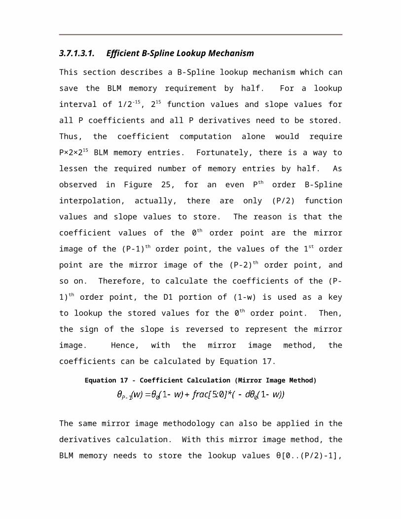
the multiplication. Since the precision of the QMM is limited to {14.10} SFXP, it is adequate to set the precision of force accumulation to {22.10} SFXP which accommodates the entry width of the PIM memory.

Table 13 - FC Arithmetic Stages (For the X Directional Force)

Name Input a Input b Output

Multi_st1thetaY {1.21} SFXP

x thetaZ {1.21} SFXP

Rounded to {1.21}

Multi_st2charge {5.21} SFXP

x dthetaX {1.21} SFXP

Rounded to {5.21}

Multi_st3 thetaY×thetaZ x charge×dthetaX Rounded to

{5.21}

Multi_st4QMM

{14.10} SFXP

x (thetaY×thetaZ) × (charge×dthetaX)

Rounded to {19.21}

Adder (Force) Force - QMM×theta×theta×charge

×dthetaRounded to

{22.10}

3.10. Parallelization StrategyIn the above sections, detailed information of the chip-level and the block-level operations are given. This section describes a strategy to parallelize the SPME reciprocal sum calculation into multiple RSCEs. It also discusses the data communication requirement among the RSCEs and also the synchronization ability of the RSCE, which is necessary for the parallelization. The parallelization strategy described in this section is very similar to the way NAMD parallelizes its reciprocal sum computation [4, 35].

3.10.1. Reciprocal Sum Calculation using Multiple RSCEsTo illustrate the basic steps involved in the parallelization strategy, a 2D simulation system example is assumed and is shown in Figure 44. In this 2D simulation system, the mesh size is KX×KY=8×8, the number of particles is N=6, the interpolation order is P=2, and the number of RSCEs is NumP=4.

Figure 44 - 2D Simulation System with Six Particles

In realizing the parallelization implementation, each RSCE should be coupled with the same five memory banks as in the single RSCE case.

They are, namely, the PIM, the BLM, the ETM, the QMMR and the QMMI memory banks. In the following paragraphs, the general idea of the parallelization steps for a 2D simulation system is explained.

To parallelize the calculation, each RSCE is assigned a portion of the mesh at the beginning of a simulation timestep. The simplest parallelization is achieved by assigning the same number of grid points to each RSCE. Hence, each RSCE is assigned KX×KY/NumP grid points, which are used for the mini-mesh composition. Since KX

and KY are in a power of 2, the value NumP should be an even number to allow an even grid point distribution. Since each RSCE can have a different number of particles to process, synchronization among the RSCEs is needed at the intermediate calculation steps. Due to the fact that system being simulated is charge-neutral (an Ewald Summation prerequisite) and is in an equilibrium state, each RSCE should handle almost the same number of particles.

After the grid-point assignment, each RSCE is responsible for the B-Spline coefficients calculation and mesh composition for all charges that are either inside its mini-mesh area or are P/2 grid points away from its mesh boundary. The mini-mesh assignment and its boundary are indicated by the dashed line in Figure 45. A special case happens when a particle interpolates its charge to P×P×P grid points that belong to several different mini-meshes. As illustrated in Figure 45, the weights of charge c are distributed to all four meshes. In this case, the influence of the charge on each mesh is calculated by the corresponding RSCE of the mesh. To avoid duplicating the weight in each mini-mesh, the wrap around handling mechanism of the RSCE is disabled in the parallelization case. With the wrap around mechanism disabled, a particle on the left edge of the mini-mesh will not have its charge interpolated to the right edge of the mini-mesh. The reason is

that the wrapped around charge weight should already be taken care of by the neighboring RSCEs.

Figure 45 - Parallelize Mesh Composition

To realize the grid point distribution step, the host only programs the PIM memory with the coordinates and charges of the particles that the RSCE is responsible for. Furthermore, the host also sets the correct number of particles N. The BLM memory is programmed with the full content as in the single RSCE case. Upon finishing the coefficient calculation and mesh composition, each RSCE holds the content of its own mini-mesh in the QMMR memory and then it halts until all RSCEs finish their own mini-mesh composition; this is the first synchronization point. In the RSCE, a programmable control register is provided to control the advancement of the calculation states. For example, the RSCE can be programmed such that its operation will be halted after the mesh composure state and it will only go to the next state (3D-IFFT state) when the control register is programmed with a proper value.

The next step is the inverse 2D-FFT operation. In this operation each RSCE is responsible for (KX×KY/NumP) grid points as well. However,

instead of holding the data for the mini-mesh, each RSCE holds grid-point data for the FFT rows it is responsible for. Thus, before performing the IFFT, data communication is needed among all RSCEs. In our 2D example, the 2D-IFFT is broken down into 2 passes of 1D FFT. For the x direction, as shown in Figure 46, each RSCE holds the data for KY/NumP rows in which each row has KX grid points. After the x direction FFT is done, synchronization is needed to ensure all RSCEs finish the first 1D FFT. Then, data communication is again necessary to transpose the data before the 1D FFT for the y direction can take place. As shown in Figure 47, for the y direction, each RSCE holds KX/NumP columns. Similar to the single RSCE case, the energy calculation (EC) can be overlapped with the 1D FFT for the last dimension. Thus, at the end of the y direction 1D-FFT step, each RSCE has calculated the energy contribution of its grid-point rows and also updated the QMMR and QMMI memories. The total reciprocal energy can then be calculated by adding the calculated energy from all RSCEs.

Figure 46 - Parallelize 2D FFT (1st Pass, X Direction)

Figure 47 - Parallelize 2D FFT (2nd Pass, Y Direction)

Following the inverse transformation, the forward 2D-FFT can be performed on the updated grid. The data communication requirement is the same as that of the 2D-IFFT step. To save one transposition, the forward 2D-FFT can be performed in reverse order. That is, the 1D-FFT for the y direction is done before that of x direction. Again, synchronization is needed in between the 1D-FFT passes.

After the forward 2D-FFT operation is done, another synchronization and data communication is needed among all RSCEs. Before the force calculation can proceed, each RSCE should hold the grid-point data of its previously assigned mini-grid. Figure 48 illustrates the data

distribution. The operation of the force calculation is similar to that of the single RSCE case, that is, it interpolates the force from the grid points back to the particles. After the calculation, each RSCE writes the calculated forces into the PIM memory. For a particle (e.g. particle c) that interpolates its charge to several RSCEs, its force is calculated by a summation of the calculated forces from all RSCEs. This summation is carried out by the host after all RSCEs report the partial forces of the particle.

Figure 48 - Parallelize Force Calculation

As observed from the above steps, the sizes of the memories for each RSCE can be reduced when multiple RSCEs are used. Firstly, the PIM memory needs only hold the data for approximately N/NumP particles. Secondly, the QMMR and QMMI memories need only hold the grid-point values for the mini-mesh or the FFT rows. Thirdly, the ETM memory need only hold the energy term that corresponds to the grid points of the mini-mesh. However, the BLM memory has to hold the same amount of data as the single RSCE case.

With the described parallelization strategy, there is a restriction on the number of RSCEs that the computations can be parallelized to.

The reason is that when performing the FFT, it is more efficient for a RSCE to hold all grid-point data for the FFT rows. The simplest configuration is to set NumP=K such that each RSCE can perform the FFT for a 2-D plane. On the other hand, if NumP is set to K×K, then each RSCE can perform the FFT for one row. The total amount of data to be transferred and the scalability in each calculation step are summarized in Table 14. In Table 14, the data communication requirement listed is intended for a 3D simulation system.

Table 14 - 3D Parallelization DetailOperation Description Total Data

TransferScale

Host computer distributes the mini-mesh to all RSCEs.

Calc. Each RSCE composes its own mini-mesh. NumP

Sync.

Comm.Data transfer is required before the 3D-IFFT can start such that each RSCE has KY×KZ/NumP KX-point rows. There is no imaginary data at this point.

KX×KY×KZ

×Grid Precision

NumP

Calc. The 1st pass 1D-IFFT is for X direction. NumP

Sync.

Comm.Data communication is required before the Y direction IFFT can start such that each RSCE has KX×KZ/NumP KY-point rows.

2×KX×KY×KZ

×Grid Precision

NumP

Calc. The 2nd pass 1D-IFFT is for Y direction. NumP

Sync.

Comm.Data communication is required before the Z direction IFFT can start such that each RSCE has KX×KY/NumP KZ-point rows.

2×KX×KY×KZ

×Grid Precision

NumP

Calc. The 3rd pass 1D-IFFT is for Z direction. NumP

Sync. Energy computation done.

Calc. The 1st pass 1D-FFT is for Z direction. NumP

Sync.

Comm.Data communication is required before the Y direction FFT can start such that each RSCE has KX×KZ/NumP KY-point rows.

2×KX×KY×KZ

×Grid Precision

NumP

Calc. The 2nd pass 1D-FFT is for Y direction. NumP

Sync.Comm. Data communication is required before the X 2×KX×KY×KZ Num

direction IFFT can start such that each RSCE has KY×KZ/NumP KX-point rows.

×Grid Precision P

Calc. The 3rd pass 1D-FFT is for X direction. NumP

Sync.

Comm.Data communication is required before the force calculation can start such that each RSCE owns its previously assigned mini-mesh. There is no imaginary grid data.

KX×KY×KZ

×Grid Precision

NumP

Calc. Each RSCE performs force calculation on its own mini-mesh and write in to the PIM memory.

NumP

Sync. Force computation is done.

Chapter 44. Speedup EstimationThis chapter provides an estimate on the degree of speedup the RSCE can provide against the SPME software implementation running at a 2.4 GHz Intel P4 computer [8]. Firstly, it explains the limitations of the current RSCE implementation on the Xilinx multimedia board. Then, it proposes a better RSCE implementation assuming that the hardware is customized to the exact requirements of the RSCE architecture. Lastly, this chapter ends with an estimate on the degree of speedup the “better” RSCE implementation can provide.

4.1. Limitations of Current ImplementationThe RSCE is currently implemented using the Xilinx multimedia board. The board has a Xilinx XC2V2000 FPGA and five independent banks of 512K x 36-bit 130MHz ZBT memory. According to the Xilinx datasheet [39], the Virtex-II XC2V2000 FPGA has 10752 slices of logic, 56 18-bit wide dedicated multipliers, and 56 18 K-bit block RAMs. The current RSCE implementation uses approximately 88% of the logic resource available in the XC2V2000 FPGA. The high percentage of logic resource usage limits the performance of the current hardware implementation in two main ways. Firstly, the high slice usage means that adding new logic to enhance the current RSCE design is impossible. Secondly, the high resource usage limits the maximum operating frequency to 40MHz. The reason is that the high slice usage makes it impossible for the place and route (P&R) to achieve a higher clock speed. Since the MicroBlaze OPB is operating at 27MHz, the current implementation is chosen to operate at 27MHz

such that no clock crossing FIFO is needed to transfer data between the MicroBlaze and the RSCE design.

Due to the lack of logic resources, there are four main design drawbacks in the current implementation. First of all, the B-Spline coefficients calculation and the mesh composition do not overlap with each other. Similarly, the B-Spline derivatives computation does not overlap with the reciprocal force calculation. Overlapping these calculations should shorten the computational time substantially. However, that would need extra logic and BRAMs to double buffer the coefficients and their respective derivatives.

Secondly, the reciprocal force calculation for the x, y, and z directions is done sequentially. These forces can be calculated in parallel to achieve maximum speedup. However, this parallelization needs approximately another 30 18-bit dedicated multipliers and around 2000 slices to realize the other two force calculation pipelines.

Thirdly, the current 3D-FFT block instantiates one Xilinx radix-2 burst I/O FFT LogiCore which, among all implementation choices, takes the longest time to perform the FFT. Based on the Xilinx Virtex-II FFT datasheet [38], the fastest pipelined streaming I/O FFT core implementation can perform a 64-point FFT in 64 clock cycles while the minimum resource radix-2 burst I/O FFT core takes 335 clock cycles. This is a slow down of five times. The reason for choosing the radix-2 burst I/O FFT core implementation is mainly due the scarcity of logic resources. As an example, a 256-point radix-2 minimum resource FFT core needs only 752 slices, three BRAMs and three 18x18 multipliers in a Virtex-II device to implement; while a 256-point pipelined streaming I/O radix-2 FFT core could need 1944 slices, four BRAMs, and 12 18x18 multipliers to implement.

Lastly, another drawback is that there is only one set of QMM memory in the current implementation. For a large number of particles, increasing the number of QMM memories can substantially speedup the calculation time during the mesh composition, the FFT transformation, and the force computation steps. More discussion on the usage of multiple QMM memories is given in Section 4.2.2.

In addition to the logic resource scarcity, the speed grade of the XC2V2000 on the board also limits the performance of the current RSCE implementation. The speed grade of the current FPGA is 4, which is the slowest speed grade for the Virtex-II family. According to the synthesizer’s results, using a speed grade of 6 can provide approximately 10% increase in the maximum operating frequency.

4.2. A Better ImplementationBased on the drawbacks of the current implementation, a better RSCE design should have the following improvements:1. Overlapping of the BCC calculation with the MC/FC calculations.2. Parallelization of the x, y, and z directional forces calculations.3. Utilization of the fastest FFT LogiCore: radix-2 pipelined streaming

I/O FFT LogiCore.4. Utilization of multiple sets of QMM memories.5. Utilization of an FPGA with higher speed grade or even better

technology.

4.3. RSCE Speedup Estimation of the Better ImplementationBased on Table 2 in Chapter 3, Table 15 lists the calculation steps along with their corresponding required number of clock cycles for the better implemented RSCE. In the table, N is the number of particles, P is the interpolation order, and K is grid size. The number of clock cycles required for each step is estimated based on its computational complexity and the implementation details of the better RSCE. The simulation waveforms of the individual design blocks are also used in the estimation. Furthermore, it is assumed that only one set of the QMMR and QMMI memories is used.

Table 15 - Estimated RSCE Computation Time (with Single QMM)

# Block Operation Estimated # of Clocks

1 BCC B-Spline coefficients lookup and calculation. This step involves reading from the PIM memory, looking up the BLM memory, and writing the calculated coefficients to the block RAMs.

N×(4+2×3×P+3×P) Overlap with MC.

2 MC Mesh Composition.This step involves reading from the QMMR memory, calculating the new QMMR values, and writing the updated values back to the QMMR memory.

N×(P×P×P×2)

3 3D-IFFT

3D-FFT Transformation. This step involves repetitively reading row data from the QMMR and QMMI memories, performing 1D-FFT, and writing the transformed data back to the QMM memories. According to the Xilinx FFT LogiCore datasheet [38], the pipelined streaming I/O FFT LogiCore takes N clock cycles to perform an N-point FFT. Therefore, TROW_TRANS = K.

3×K×K×(TROW_TRANS

+K)

4 EC Energy Computation. This step involves reading from the ETM memory, multiplying the energy term of the grid point with the corresponding grid point value in the QMMR/I memories, and writing the updated values back to the QMMR/I memories.

K×K×KOverlap with the last pass of 2D-FFT.

5 3D-FFT 3D-FFT Transformation. 3×K×K×(TROW_TRANS

+K)

6 BCC B-Spline coefficients and derivatives lookup and calculation.

N×(4+2×3×P+3×P) Overlap with FC.

7 FC Force Computation. This step involves reading from the QMMR memory, calculating the directional forces, and writing the calculated forces to lower half of the PIM.

N×P×P×P

According to Table 15, the total computation time can be estimated with Equation 23. The computation time tMC and tFC scale with the values N and P; while the computation time t3D-IFFT and t3D-FFT scale with the value K.

Equation 23 - Total Computation Time (Single-QMM RSCE)

4.3.1. Speedup with respect to a 2.4 GHz Intel P4 ComputerThis section provides an estimate on the level of speedupdegree of speedup the RSCE can provide in the SPME reciprocal sum computations. Since the RSCE is expected to be used to accelerate MD simulation of molecular systems that contain at most tens of thousands of particles, the estimate provided in this section is limited to a maximum N=20000. To provide the estimate, the single-timestep computation time of the better implemented RSCE (assuming it is running at 100MHz*) is compared with that of the SPME software implementation [8] running in a 2.4 GHz P4 computer with 512MB DDR RAM. Table 16 shows the RSCE speedup for MD simulations when the number of particles N=2000 and N=20000.

*Note: Current RSCE implementation (without the MicroBlaze softcore) in the Xilinx XCV2000-4 has a maximum clock frequency of ~75MHz.

Table 16 - Speedup Estimation (RSCE vs. P4 SPME)

N P K BCC MC FFT EC FC Total

RSCE 2000 4 32 0.00E+00

2.56E-03

3.93E-03

0.00E+00

1.28E-03

7.77E-03

Software

2.20E-03

8.41E-03

3.30E-02

1.18E-02

9.23E-03

6.46E-02

Speedup 3.28 8.46 7.21 8.32

RSCE 2000 4 64 0.00E+00

2.56E-03

3.15E-02

0.00E+00

1.28E-03

3.53E-02

Software

2.18E-03

2.26E-02

3.16E-01

9.44E-02

1.10E-02

4.47E-01

Speedup 8.82 10.06 8.62 12.65

RSCE 2000 4 128

0.00E+00

2.56E-03

2.52E-01

0.00E+00

1.28E-03

2.55E-01

Software

2.22E-03

1.10E-01

2.87E+00

7.50E-01

1.35E-02

3.74E+00

Speedup 42.80 11.39 10.55 14.65

RSCE 2000 8 32 0.00E+00

2.05E-02

3.93E-03

0.00E+00

1.02E-02

3.47E-02

Software

6.36E-03

4.57E-02

3.31E-02

1.19E-02

6.26E-02

1.60E-01

Speedup 2.23 8.41 6.11 4.60

RSCE 2000 8 64 0.00E+00

2.05E-02

3.15E-02

0.00E+00

1.02E-02

6.22E-02

Software

6.40E-03

6.66E-02

3.14E-01

9.43E-02

7.33E-02

5.55E-01

Speedup 3.25 9.99 7.16 8.92

RSCE 2000 8 128

0.00E+00

2.05E-02

2.52E-01

0.00E+00

1.02E-02

2.82E-01

Software

6.36E-02

1.67E-01

2.50E+00

7.15E-01

5.71E-02

3.50E+00

Speedup 8.14 9.93 5.57 12.40

RSCE 20000 4 32 0.00E+

002.56E-

023.93E-

030.00E+

001.28E-

024.23E-

02Software

2.39E-02

6.72E-02

3.33E-02

1.18E-02

9.41E-02

2.30E-01

Speedup 2.63 8.46 7.35 5.44

RSCE 20000 4 64 0.00E+

002.56E-

023.15E-

020.00E+

001.28E-

026.99E-

02Software

1.64E-02

7.66E-02

2.48E-01

7.30E-02

7.26E-02

4.87E-01

Speedup 2.99 7.89 5.67 6.97

RSCE 2000 4 12 0.00E+ 2.56E- 2.52E- 0.00E+ 1.28E- 2.90E-

0 8 00 02 01 00 02 01Software

1.86E-02

1.73E-01

2.23E+00

5.92E-01

9.26E-02

3.10E+00

Speedup 6.77 8.85 7.23 10.70

RSCE 20000 8 32 0.00E+

002.05E-

013.93E-

030.00E+

001.02E-

013.11E-

01Software

6.35E-02

4.26E-01

3.30E-02

1.18E-02

6.24E-01

1.16E+00

Speedup 2.08 8.38 6.09 3.72

RSCE 20000 8 64 0.00E+

002.05E-

013.15E-

020.00E+

001.02E-

013.39E-

01Software

6.35E-02

5.51E-01

3.12E-01

9.39E-02

7.32E-01

1.75E+00

Speedup 2.69 9.93 7.15 5.17

RSCE 20000 8 12

80.00E+

002.05E-

012.52E-

010.00E+

001.02E-

015.59E-

01Software

6.36E-02

7.69E-01

2.37E+00

6.67E-01

5.65E-01

4.44E+00

Speedup 3.76 9.43 5.52 7.94

As shown in Table 16, the RSCE speedup ranges from a minimum of 3x to a maximum of 14x. Furthermore, it is observed that the RSCE provides a different level of speedupdegree of speedup depending on the simulation setting (K, P, and N). One thing worthwhile to notice is that when N=2000, P=4, and K=128, the speedup for the MC step reaches 42x. One of the reasons for this high level of speedupdegree of speedup is that when grid size K=128, the number of elements in the Q charge array would be 128×128×128=2097152; this large array size limits the performance advantage of using cache in a computer.

The speedup increases with the increasing grid size K. The reason is that the RSCE fixed-point 3D-FFT block provides a substantial speedup (>8x) against the double precision floating-point 3D-FFT subroutine in the software. Furthermore, since the EC step in the RSCE is overlapped with the 3D-FFT step, it theoretically costs zero

computation time. Therefore, the EC step, which scales with K, also contributes to the speedup significantly when the grid size K is large. On the other hand, the speedup decreases with increasing number of particles N and interpolation order P. The reason is that when N and P is large, the workload of the MC step starts to dominate and the speedup obtained in the 3D-FFT step and the EC step is averaged downward by the speedup of the MC step (~2x when N is large). That is, the MC workload is dominant when the imbalance situation described in Equation 24 happens.

Equation 24 - Imbalance of Workload

Hence, it can be concluded that when N×P×P×P is large relative to the value of K×K×K, the speedup bottleneck is in the MC step. It seems obvious that more calculation pipelines in the MC step can mitigate this bottleneck. Unfortunately, the QMM bandwidth limitation defeats the purpose of using multiple MC calculation pipelines. More discussion on the characteristics of the RSCE speedup and the relationship among the values of K, P and N is provided in Section 4.4.

Comparing with the other hardware accelerators [23, 26], the speedup of the RSCE is not very significant. There are two main factors that are limiting the RSCE from achieving a higher level of speedupdegree of speedup; they are the limited access bandwidth of the QMM memories and the sequential nature of the SPME algorithm. In all the time consuming steps (e.g. MC, 3D-FFT, and FC) of the reciprocal sum calculations, the QMM memories are accessed frequently. Therefore, to mitigate the QMM bandwidth limitation and to improve the level of speedupdegree of speedup, a higher data rate

memory (e.g. Double Data Rate RAM) and more sets of QMM memories can be used.

4.3.2. Speedup Enhancement with Multiple Sets of QMM MemoriesTo use multiple sets of QMM memories to increase the RSCE to QMM memory bandwidth, design modifications are inevitable in the MC, the 3D-FFT, and the FC design block. To help explain the necessary modifications, let’s assume that the interpolation order P is 4, the grid size K is 16, and that four QMMR and four QMMI memories are used (i.e. NQ = 4).

Firstly, during the MC step, for each particle, the RSCE performs Read-Modify-Write (RMW) operations using all four QMMR simultaneously. Therefore, four MC calculation pipelines are necessary to take advantage of the increased QMM bandwidth. For example, for P=4, there are 4×4×4 = 64 grid points to be updated. Therefore, each QMMR memory will be used for updating 16 grid points. After all particles have been processed, each QMMR memory holds a partial sum of the mesh. Hence, a global summation operation can be performed such that all four QMMR memories will hold the final updated mesh. With four QMMR memories, the mesh composition would take approximately (N×P×P×P×2)/4 + 2×K×K×K clock cycles to finish; the second term is for the global summation. That is, it takes K×K×K clock cycles to read all grid point values from all the QMMs and it takes another K×K×K clock cycles to write back the sum to all QMM memories. For a large number of particles N, an additional speedup close to 4x can be achieved. The maximum number of the QMM memories to be used is limited by the number of FPGA I/O pins and the system cost.

In addition to speeding up the MC step, using multiple QMM memories can speedup the 3D-FFT step as well. In the multiple QMM memories case, each set of the QMMR and the QMMI is responsible for (K×K)/4 rows of the 1D-FFT. Hence, to match the increased QMM memories access bandwidth, four K-point FFT LogiCores should be instantiated in the 3D-FFT design block. After each pass of the three 2D-FFT transformations is finished, a global data communication needs to take place such that all QMM memories get the complete 2D-FFT transformed mesh. This process repeats until the whole mesh is 3D-FFT transformed. By using four sets of QMMR and QMMI, the 3D-FFT step takes 3×(K×K× (TROW_TRANS+ K)/4 + 2×K×K×K) clock cycles to complete. The second term represents the clock cycles the RSCE takes to perform the global communication.

Lastly, the force computation step can also be made faster using multiple sets of the QMM. After the 3D-FFT step, each of the four QMMR should hold the updated grid point values for calculating the directional forces. For each particle, the RSCE shares the read accesses for the grid point values among all four QMMR memories; this effectively speeds up the force computations by a factor of four. Table 17 and Equation 25 show the estimated computation time for the RSCE calculation when multiple sets, NQ, of the QMM memories are used.

Table 17 - Estimated Computation Time (with NQ-QMM)

# Design Block

Operation Estimated # of Clocks

1 BCC B-Spline coefficients calculation.

Overlapped.

2 MC Mesh Composition. N×(P×P×P×2)/NQ + 2×K1×K2×K3

3 3D-IFFT 3D-FFT 3×(K×K× (TROW_TRANS+ K)/ NQ +

Transformation. 2×K×K×K)4 EC Energy Computation. Overlapped.5 3D-FFT 3D-FFT

Transformation. 3×(K×K× (TROW_TRANS+ K)/NQ + 2×K×K×K)

6 BCC B-Spline coefficients & derivatives calculation.

Overlapped.

7 FC Force Computation. N×P×P×P/NQ

Equation 25 - Total Computation Time (Multi-QMM RSCE)

Based on Table 17 and Equation 25, the usage of multiple QMMs should shorten the RSCE computation time the most when the grid size (K) is small, the number of particles (N) is large, and the interpolation order (P) is high. The speedup plots of using four QMMs versus one QMM are shown in Figures 49, 50 and 51. In Figures 49 and 50, it is shown that a smaller value of grid size K favors the multi-QMM speedup. As an example, when K=32, a speedup of 2x realized when N=2.0x103; while for K=128, the same speedup is realized at a much larger N=1.30x105. The reason for this behavior is that the required global summation starts to take its toll when the grid size K is a large number.

Multi-QMM RSCE Speedup against 1-QMM RSCE

0.00

0.50

1.00

1.50

2.00

2.50

3.00

3.50

4.00

4.50

0.00E+00 5.00E+04 1.00E+05 1.50E+05 2.00E+05

N

Mul

ti-Q

MM

RSC

E vs

1-Q

MM

RSC

E Sp

eedu

pP=4, K=32 P=4, K=64 P=4, K=128 P=4, K=256

Figure 49 - Speedup with Four Sets of QMM Memories (P=4).

M ulti-QM M RSCE Speedup against 1-QMM RSCE

0.00

0.50

1.00

1.50

2.00

2.50

3.00

3.50

4.00

4.50

0.00E+00 5.00E+04 1.00E+05 1.50E+05 2.00E+05

N

Mul

ti-Q

MM

RS

CE

vs

1-Q

MM

RS

CE

Spe

edup P=8, K=32 P=8, K=64 P=8, K=128 P=8, K=256

Figure 50 - Speedup with Four Sets of QMM Memories (P=8).

On the other hand, as shown in Figure 51, a higher interpolation order favors the multi-QMM speedup. For a grid size K=64, when

P=4, the usage of multiple QMMs provides a 3x speedup when N=1x105; while for P=8, the same speedup happens when N=1.0x104.

Effect of Interpolation Order P on Multi-QMM RSCE Speedup

0.00

0.50

1.00

1.50

2.00

2.50

3.00

3.50

4.00

4.50

0.0E+00 5.0E+04 1.0E+05 1.5E+05 2.0E+05

N

Mul

ti-Q

MM

RSC

E vs

. 1-Q

MM

RSC

E Sp

eedu

p P=4, K=64 P=8, K=64

Figure 51 - Speedup with Four Sets of QMM Memories (P=8, K=32).

4.4. Characteristic of the RSCE SpeedupIn Section 4.3.1 and Section 4.3.2, it is estimated that the single-QMM RSCE can provide a speedup ranging from 3x to 14x while the usage of a multi-QMM is able to provide an additional speedup with an upper bound of NQ which represents the number of QMM the RSCE uses. In both the single-QMM and the multi-QMM cases, the magnitude of RSCE speedup varies with the values of K, P, and N. Therefore, depending on the simulation setting (K, P, and N), the total speedup of using the multi-QMM RSCE can range from the worst case of 3x to the best case of slightly less than NQ×14x. The following table shows how the simulation setting affects the single-QMM and the multi-QMM speedup.

Table 18 - Variation of Speedup with different N, P and K.Single-QMM Speedup

Multi-QMM Speedup

MD Sim. Accuracy

Number of Particles: N ↑

↓ ↑ N/A

Interpolation Order: P ↑

↓ ↑ ↑

Grid Size K ↑

↑ ↓ ↑

As indicated in the table, the single-QMM RSCE provides the best speedup when N is small, P is small, and K is large. On the other hand, the multi-QMM RSCE provides the best speedup when N is large, P is large and K is small. In a typical MD simulation, the user would choose the grid size K and the interpolation order P to control the simulation accuracy. A higher grid density and a higher interpolation order P would lead to a more accurate MD simulation. Therefore, to obtain an accurate simulation result, the value of K and P should be increased correspondingly. Furthermore, as stated by Darden [2], in an MD simulation using the PME algorithm, for any desirable accuracy, the total number of grid points (KX×KY×KZ) should

be of the same order as the number of particles N. Hence, the values K, P, and N should be related to one another.

When the N is of the same order as (KX×KY×KZ), the usage of NQ-QMMs does provide a consistent speedup of close to NQ. As shown in Figure 52, when the value KX×KY×KZ is of the same order as N, the NQ=4 QMMs speedup is only affected by the interpolation order P. For example, with an interpolation order P of 4, the usage of four QMMs provides a speedup of 3.58. In Figure 52, the N is simply calculated as K×K×K.

Multi-QMM RSCE Speedup against 1-QMM RSCE(when K*K*K is of the same order as N)

32

168

3.00

3.20

3.40

3.60

3.80

4.00

4.20

0 20000 40000 60000 80000 100000

N

Mul

ti-Q

MM

RSC

E Sp

eedu

p

0

10

20

30

40

50

60

Grid

Siz

e K

P=4 P=8 P=12 Value of K

Figure 52 - Effect of the Interpolation Order P on Multi-QMM RSCE Speedup

(When K×K×K is of the Same Order as N)

Based on the assumption that the number of grid points is of the same order as the number of particles and the simulation results presented in Table 16 and Figures 49 to 52, the worst case speedup of a single-

QMM RSCE can be estimated to be 3-fold while that of the multi-QMM RSCE can be approximated to be around (NQ-1)×3. The factor (NQ-1) is approximated by locating the worst case speedup when K×K×K is of the same order as N in Figure 49. For example, when K=32 (K×K×K=32768), the range of N used to search for the worst case speedup is from 10000 to 99999.

To show the overall speedup of the multi-QMM RSCE against the software implementation running at the 2.4GHz Intel P4 computer, the single-QMM RSCE speedup data from Table 16 and the data used to plot Figures 49 and 50 are used to estimate the overall speedup. The 4-QMM RSCE speedup results are shown in Table 19. As seen in the table, the 4-QMM RSCE can provide a 14x to 20x speedup over the software implementation (based on the simulated cases). One thing worthwhile to notice is that when there is no relationship among the values of K, P and N, although the multi-QMM increases the speedup lower bound from 3x to 14x, it does not increase the maximum speedup significantly (increase from 14x to 20x). This can be explained by the fact that the single-QMM RSCE speedup and the multi-QMM RSCE speedup vary differently with the three simulation parameters (K, P, and N). The difference is shown in Table 18.

Table 19 - Speedup Estimation (Four-QMM RSCE vs. P4 SPME)

N P KSingle-QMM

Speedup againstSoftware Running @

Intel P4

Four-QMMSpeedup againstSingle-QMM

Four-QMMSpeedup against

Software

Speedup

2000 4 32 8.32 1.99 16x

Speedup

2000 4 64 12.65 1.44 18x

Speedup

2000 4 12

8 14.65 1.37 20x

Speedup

2000 8 32 4.60 3.26 15x

Speedup

2000 8 64 8.92 1.99 17x

Speedup

2000 8 12

8 12.40 1.44 17x

Speedup

20000 4 32 5.44 3.37 18x

Speedup

20000 4 64 6.97 2.10 14x

Speedup

20000 4 12

8 10.70 1.46 15x

Speedup

20000 8 32 3.72 3.90 14x

Speedup

20000 8 64 5.17 3.37 17x

Speedup

20000 8 12

8 7.94 2.10 16x

4.5. Alternative ImplementationRather than speeding up the whole SPME algorithm in hardware, an alternative is to only speedup the 3D-FFT operation in a dedicated high performance FFT co-processor. This alternative architecture is shown in Figure 53.

Figure 53 - CPU with FFT Co-processor

To investigate the speedup potential of the FFT co-processor architecture, the SPME computational complexity estimation in Table 2 is used. The SPME computational complexity is summarized in Equation 26 for easy reference.

Equation 26 - SPME Computational Complexity (Based on Table 2)

To determine the maximum achievable speedup of the FFT co-processor architecture, the infamous Amdahl’s Law [40] is applied by assuming the FFT co-processor can compute the 3D-FFT and the 3D-IFFT in zero time. Based on Equation 26, Table 20 shows the number of computation cycles involved in the SPME computation with and without the 3D-FFT operation. Furthermore, the table also shows the degree of speedup of the FFT co-processor architecture for different grid sizes K. In generation of the speedup data, it is assumed that the number of particles N is one half of the total number of grid points K×K×K and the interpolation order P equals to 4. As shown in the table, if only the FFT operation is accelerated (to have a computation cycle of zero), the degree of speedup for the FFT co-processor architecture is still very insignificant (< 2x). The main reason is that the B-Spline calculation, the mesh composition, the energy calculation, and the force calculation cannot be overlapped in a CPU and they constitute a large portion of the SPME computation time. Therefore, to accelerate the SPME computation, all major computation steps should be accelerated.

Table 20 - Speedup Potential of FFT Co-processor Architecture

K N PTotal SPME

Cycles3D-FFT Cycles

Total SPME Cycle

(Without 3D-FFT)

Speedup

8 256 4 8.45E+04844809.22E+0392

167.53E+047526

41.12244912

16 2048 47.00E+0570041

69.83E+0498

3046.02E+056021

121.1632

65

32 16384 45.80E+0657999

369.83E+0598

30404.82E+064816

8961.2040

82

6413107

2 44.80E+0747972

3529.44E+0694

371843.85E+073853

51681.2448

98128

1048576 4

3.96E+08396361728

8.81E+0788080384

3.08E+08308281344

1.2985714

4.6. RSCE Speedup against N2 Standard Ewald SummationWith a lower bound speedup of 3x, the speedup ability of the single-QMM RSCE is not significant. This is due to the lack of parallelism in the SPME algorithm and also due to the limited QMM memory access bandwidth. Although the impact of limited QMM bandwidth is mitigated with the usage of more QMM memories, the lack of parallelism in the SPME algorithm still bottlenecks the RSCE speedup. Furthermore, it is obvious that the Standard Ewald Summation [28, 33] is easier to implement and is also easier to parallelize [28, 33]. This leads to a question on why the SPME algorithm should be implemented in hardware instead of the Standard Ewald Summation. This question can be answered by the plot in Table 21 and Figure 54.

In the plot in Figure 54, a negative Log(Speedup) value means there is a slow-down to use the RSCE to perform the forces and energy calculations; while a positive value means a speedup. The plot uses the RSCE computation clock cycle estimation described in Equation 25 and simply takes N2 as the clock estimation for Standard Ewald Summation. The plot shows that as the number of particles N increases to a threshold point Nthreshold (the zero-crossing point in the graph), the intrinsic O(N×Log(N)) RSCE implementation starts to provide significant speedup against the O(N2) Ewald Summation algorithm. The threshold Nthreshold increases as the grid size K and interpolation order P increases. The relationship of Nthreshold and the interpolation order P is illustrated in Figure 55. Table 21 shows the threshold points for different simulation settings. As shown in the table, the RSCE starts to provide speedup against the Ewald Summation when the number of particles N is fairly small.

Table 21 - RSCE Speedup against Ewald Summation

Simulation Setting

Minimum N to Observe a Speedup (Nthreshold)

P=4, K=32 700P=4, K=64 3500P=8, K=64 5000

P=4, K=128 7000P=4, K=256 13000

1-QMM RSCE Speedup against N^2 Ewald Summation

-3.00

-2.00

-1.00

0.00

1.00

2.00

3.00

4.00

0.00E+00 2.00E+04 4.00E+04 6.00E+04 8.00E+04 1.00E+05 1.20E+05

N

Log

(1-Q

MM

RSC

E Sp

eedu

p ag

ains

t E.S

.)

P=4, K=32 P=4, K=64 P=4, K=128 P=4, K=256

Figure 54 - Single-QMM RSCE Speedup against N2 Standard Ewald

Effect of Interpolation Order P on 1-QMM RSCE Speedup

-1.000

-0.500

0.000

0.500

1.000

1.500

2.000

2.500

3.000

3.500

0.00E+00 5.00E+04 1.00E+05 1.50E+05

N

Log

(Sin

gle-

QM

M R

SCE

Spee

dup

agai

nst E

wal

d Su

mm

atio

n)P=4, K=64 P=8, K=64

Figure 55 - Effect of P on Single-QMM RSCE Speedup

Figure 56 plots the RSCE speedup against the Ewald Summation when the number of particles N is of the same order as the number of grid points K×K×K. This eliminates the speedup dependency of the varying N and varying K. As observed in the plot, the N threshold

increases with increasing interpolation order P. Table 22 summarizes the result.

Table 22 - RSCE Speedup against Ewald Summation (When K×K×K = ~N)

Interpolation Order P

Nthresh

old4 2008 1584

12 5012

1-QMM RSCE Speedup against Ewald Summation (when K*K*K is of the same order as N)

-3

-2

-1

0

1

2

3

4

5

6

7

0 1 2 3 4 5 6 7 8 9

Log(N)

Log(

RSC

E Sp

eedu

p ag

ains

t E.S

.)

P=4 P=8 P=12

Figure 56 - RSCE Speedup against the Ewald Summation (When K×K×K is of the same order as N)

4.7. RSCE Parallelization vs. Ewald Summation ParallelizationUp to now, when performing the calculations for the Coulombic interactions under the periodic boundary condition, all hardware MD systems [23, 28] chose to implement and parallelize the Ewald Summation. There is no significant effort to implement and parallelize the SPME algorithm in hardware. During the development stage of this thesis, there are several observations that may help explain this trend.

Firstly, the SPME algorithm itself is more difficult to implement in hardware than the Ewald Summation. Although the calculations for the direct sum in the SPME algorithm and in the Ewald Summation are identical, the difference is in the reciprocal sum calculations. The reciprocal sum calculation in the SPME is difficult because it involves some complex mathematical operations such as the B-Spline interpolation and the 3D-FFT. In addition to their implementation difficulty, these mathematical operations also complicate the analytical precision analysis on the fixed-point arithmetic typically used in hardware.

Secondly, the SPME algorithm is a sequential algorithm in which the energy and forces are computed with a sequence of calculation steps. Although several calculation steps can be overlapped, this sequential characteristic of the SPME algorithm still prohibits the full exposure to the FPGA parallelization capability. One of the main reasons that the hardware implementation of the SPME algorithm needs to be sequential is that in each calculation step, the QMM grid needs to be updated before the next step can proceed. For example, the 3D-IFFT

operation cannot be started before the MC block finishes composing the QMM grid.

Thirdly, on a system-level view, if the reciprocal sum calculation is parallelized to multiple FPGAs, the data communication requirement of the SPME algorithm is more demanding than that of the Ewald Summation. With the Ewald Summation, a replicated data scheme (that is each FPGA holds the information for all N particles) can eliminate the data communication requirement during the energy and force calculation. However, with the SPME algorithm, there is no obvious way to eliminate the data communication requirement. The reason is that the data communication among multiple FPGAs is needed to exchange the updated QMM grid information in the intermediate steps.

Lastly, while the opportunity of parallelization in the Ewald Summation is limited by the number of particles N, the opportunity of parallelization in the SPME algorithm is limited by the grid size K or the grid plane size K×K. The reason is that the FFT operation in the SPME algorithm is more efficient when each FPGA performs the FFT for a row. Therefore, the grid size K limits the maximum number of FPGAs to be used in parallelizing the SPME calculations. Table 23 shows the relationship between the grid size K and the maximum number of FPGA to be used. For a large grid size K, if each RSCE performs the FFT for a row during the 3D-FFT operation, the maximum number of RSCEs is well over ten thousands. It would be impractical and unrealistic to build a hardware system with more than ten thousands RSCEs.

Table 23 - Maximum Number of RSCEs Used in Parallelizing the SPME Calculation

Grid Size K Max. # of RSCEs Max. # of RSCEs

(Assume orthogonal box)

(Each RSCE takes a plane

during FFT)

(Each RSCE takes a row

during FFT)32 32 102464 64 4096

128 128 16384256 256 65536

Although there are limitations and difficulties in implementing and parallelizing the SPME algorithm in hardware, the main justification for implementing the SPME algorithm is the intrinsic N×Log(N) complexity of the SPME algorithm. Although this complexity benefit will be offset by the limited parallelization opportunity and data communication requirement when the number of FPGAs used increases to a certain threshold NumPthreshold, this threshold number of FPGAs is very high.

Figure 57 shows the effect of increasing the number of FPGAs on the speedup of the multi-RSCE system against the multi-FPGA Ewald Summation system. As observed in the figure, as the number of FPGAs used increases, the speedup provided by the multi-RSCE system decreases. The reason is that the data communication time, which increases with NumP, starts to takes its toll on the overall multi-RSCE performance. The zero-crossing point in the graph represents the threshold number of FPGAs NumPthreshold when the multi-FPGA Ewald Summation system starts to outperform the multi-RSCE system.

Table 24 summarizes the thresholds NumPthreshold for different grid sizes. For a grid size K=32, the NumPthreshold is 4000 and for a grid size of K=64, the NumPthreshold is as large as 33000. The threshold number of FPGAs increases with increasing grid size. Although, due to the implementation simplicity, more calculation pipelines should be

able to be fitted into an Ewald Summation FPGA, the threshold number of FPGAs is still too large for any grid size of larger than 64,. This suggests that for any realistic hardware system, the multi-RSCE system would outperform the multi-FPGA Ewald Summation system.

Table 24 - Threshold Number of FPGAs when the Ewald Summation starts to be Faster

Grid Size K(Assume

orthogonal box)

Corresponding Number of Particles N

Max. # of RSCEs

Threshold Num. of FPGAs

32 16384 1024 400064 131072 4096 33000

128 1048576 16384 1040000

Comparision of RSCE and Ewald Summation Parallelization

-1.5

-1

-0.5

0

0.5

1

1.5

2

2.5

3

0 10000 20000 30000 40000 50000 60000 70000

Number of FPGAs

Log

(Mul

ti-R

SCE

Spee

dup

agai

nst M

ulti-

E.S.

)

P=4;K=32; N=16384; Max numP=1024 P=4;K=64;N=131072;Max numP=4096P=4;K=128;N=1048576;Max numP=16384

Figure 57 - RSCE Parallelization vs. Ewald Summation Parallelization

In plotting the graph in Figure 57, several assumptions have been made. Firstly, the total number of grid points is of the same order as N [2], this provides a fair basis to compare the two algorithms. Secondly, the maximum number of FPGAs used in the SPME hardware is limited by the number of rows in the charge grid. When the number of FPGAs increases beyond the number of rows, it is assumed that the extra FPGAs will be left idle during the 3D-FFT

processes and they only will participate during the mesh composition and the force calculation stages. Thirdly, it is assumed there is no data communication requirement for the multi-FPGA Ewald Summation system, that is, the usage of data replication is assumed for the Ewald Summation hardware. Fourthly, it is assumed that the communication backbone for the multi-RSCE system is non-blocking and has a transfer rate of 2GBit/s. Lastly, in plotting the graph, the communication time and the computation time of the multi-RSCE system are estimated with Equation 27 and Equation 28.

Equation 27 - Communication Time of the Multi-RSCE System

Equation 28 - Computation Time of the Multi-RSCE System

The derivation of the equations stems from Section 3.10 of this thesis. As described in Section 3.10, there are six synchronization and communication points for the multi-RSCE operation. In two of them, only the real part of the grid (after the MC step and before the FC step) needs to be exchanged among the RSCEs, and in the remaining four of them, both the real and the imaginary part of the grid need to be exchanged. Therefore, there are altogether (10×KX×KY×KZ×PrecisionGrid) bits of data to be exchanged after each synchronization point and each RSCE should theoretically need (10×KX×KY×KZ×PrecisionGrid)/NumP bits of data for the mini-mesh or for the FFT rows it is responsible for. Furthermore, assuming that the RSCEs are organized in a 2D mesh with nearest-neighbor connection and the multi-RSCE system has intelligence to deliver data to any RSCE without blocking; the number of transmission hops for the RSCE to send a request and receive the data can be approximated to

be 2×√NumP. Therefore, the communication time can be estimated with Equation 27. On the other hand, Equation 28 is derived from the information shown in Table 14 of Section 3.10.

After the different aspects of the RSCE speedup is examined, the next chapter discusses the verification and the validation effort of the RSCE implementation.

Chapter 55. Verification and Simulation EnvironmentThis chapter details the effort of verifying the RSCE design and it also describes the SystemC simulation environment that allows studies of the RSCE calculation precision requirement. Furthermore, it also presents the result of the demo MD simulations when the RSCE is used with NAMD2 software.

5.1. Verification of the RSCEThis section discusses the RSCE design verification effort. It first describes the implementation of the RSCE SystemC model, then it describes the RSCE verification testbench, and lastly, it explains the program flow of a verification testcase.

5.1.1. RSCE SystemC ModelA SystemC model is developed to calculate the SPME reciprocal energy and forces with either fixed-point arithmetic or double precision arithmetic. The ability to use different arithmetic and precision is achieved by using the template class and functions of the C++ programming language. With the template classes and functions, the same model can be used for different data types. Furthermore, with the template specialization feature, the C++ and the SystemC functions can be mixed together to ease the implementation.

During the development of the SystemC simulation model, the golden SPME implementation is used as a reference to ensure the

correctness of the simulation model in all calculation steps. Furthermore, the SystemC model is developed to model the hardware architecture closely. The structure of the SystemC RSCE model is shown in Figure 58. As shown in the figure, the SystemC model consists of the same design blocks (BCC, MC, 3D-FFT, EC, and FC) as the hardware implementation. In this way, design or architectural issues can be investigated before the actual RTL design is implemented. Furthermore, this enhances the verification capability of the model and eases the integration of the SystemC model into the verification testbench.

Separate from the RSCE SystemC model, another SystemC model is also developed to represent the host that communicates with the RSCE to carry a single-timestep MD simulation. The host SystemC model is responsible for filling the PIM memory with the shifted and scaled fractional coordinates and the charge of the particles, the BLM memory with the B-Spline coefficients, derivatives and slope of the derivatives at the predefined lookup points, and the ETM memory with the energy term of the grid points. Once it finishes filling the memory arrays, it calls the RSCE functions to perform the timestep computation either with the user-specified fixed-point arithmetic or with the double precision floating-point arithmetic. The host SystemC model (HOST) is shown on the left side of Figure 58. As illustrated in the figure, the host SystemC instantiates an eterm calculator (ETMC) and a B-Spline Coefficient Calculator (BCC) which are responsible for filling the ETM and the BLM lookup memories respectively.

Figure 58 - SystemC RSCE Model

5.1.2. Self-Checking Design Verification TestbenchThis section describes the verification environment for the RSCE development. The testbench, the memory models and the bus functional model (BFM) are implemented in SystemC. As shown in Figure 59, the verification environment consists of the following components:1. A testcase that takes a protein data bank (PDB) file as input and

provides various configurations setting (e.g. interpolation order, grid size, etc.) and particle information to the RSCE testbench (RSCE_TB).

2. The RSCE testbench (RSCE_TB) that instantiates the BFM (opbBfm), the RTL design (through a SystemC wrapper), the memory models, the checker and the RSCE behavioral model.

3. An OPB bus functional model (opbBfm) that models the MicroBlaze OPB interface that sends the instructions to both the RSCE RTL and the RSCE behavioral model.

4. Five memory models that model the ZBT memories on board. The memory models also act as checkers to monitor and verify the memory accesses from both the RSCE RTL and the RSCE behavioral model.

5. A checker that verifies that the calculated energy and forces from the RSCE RTL are the same as the results from the behavioral model.

Figure 59 - SystemC RSCE Testbench

5.1.3. Verification Testcase FlowA verification testcase starts with the testcase reading from a test-specific PDB file for a molecular or atomic system. From the PDB file, the testcase obtains the simulation box dimension and the Cartesian coordinates and charge of all particles. On the other hand, the interpolation order and the grid size are set according to the purpose of the test.

After all test information is gathered, the testcase calls the host SystemC model to perform calculations and fill the BLM, the ETM, and the PIM SystemC memory models through a backdoor mechanism. Furthermore, the entries that constitute the charge grid in the QMMR and the QMMI memory are cleared to zero.

After all the memories are initialized, a number of OPB packets can be constructed and sent to the RSCE. These OPB packets represent transactions to program the RSCE registers and configure the RSCE to perform the reciprocal sum calculation for one timestep. The register programming sets up the interpolation order, the grid size, and the number of particles in the simulation. At the same time, an equivalent microprocessor packet (upPkt) is sent to the RSCE behavioral model to configure it for the same reciprocal sum calculation.

At this point, the computation starts and every memory transaction from the RSCE RTL is logged and checked against the behavioral model during the simulation. The testcase keeps polling the RSCE status register to check if the energy calculation is complete and if so, it then reads and checks the reciprocal energy calculated by the RSCE RTL by comparing it against energy calculated by the behavior model.

On the other hand, since the reciprocal forces are written to the lower half of the PIM memory, they should be automatically checked.

The same test flow can be used with different interpolation orders, different grid sizes, and different input PDB files and the self-checking verification testbench should still be able to verify the functional correctness of the RSCE RTL without any modification.

5.2. Precision Analysis with the RSCE SystemC ModelIn addition to being used as the behavioral model in the verification testbench, the flexible SystemC RSCE model can also be used for precision analysis. This section describes how the precision of the B-Spline calculation and the 3D-FFT calculation affects the errors of the reciprocal energy and force calculations. Furthermore, this section also states the required B-Spline and 3D-FFT calculation precision to achieve the relative energy and force error goal of less than 10 -5. The errors in the energy and forces calculations are derived by Equation 29, Equation 30, and Equation 31.

Equation 29 – Absolute Error

Equation 30 – Energy Relative Error

Equation 31 – Force RMS Relative Error

The “GOLDEN” subscript indicates that the reciprocal energy or forces are calculated with the SPME software package [8]; while the “FXPT_SC” subscript indicates that the reciprocal energy or forces are

calculated with the fixed-pointed SystemC RSCE model. Equation 30 is used for calculating the relative error in energy computation. On the other hand, Equation 31 is used for calculating the RMS relative error in forces computation.

To derive the relationship between the calculation precision and the magnitude of the relative force and energy errors, 10 single-timestep MD simulations are carried out for each precision setting and each simulation setting (K, P, and the Ewald Coefficient). A script is written to automate this precision analysis simulation process. The pseudo code of the script is shown in Figure 60. The forces and energy error in these simulations are recorded, averaged, and plotted to show the effect of calculation precision on the energy and forces errors. The system being simulated is charge-neutral and it contains 100 randomly located particles with randomized charge within the range of [5.0, -5.0]. The simulation box is orthogonal with dimensions 16.0Ao x 16.0Ao x 16.0Ao.Ewald Coefficient E = 0.30Interpolation order P = 4Grid size K = 16 NumSet = 3NumRunInSet = 10

for each FFT precision {14.18, 14.22, 14.26, 14.30}: for each FFT precision {1.21, 1.24, 1.27, 1.30}: Recompile the RSCE SystemC model with the corresponding precision. for 1 to NumSet Set E, P and K for 1 to NumRunInSet Randomize coordinates within 16.0Aox16.0Aox 16.0Ao box Randomize charges with range [-5.0, 5.0] Regenerate PDB file Run single-timestep MD simulation Record the errors end for increment E by 0.05 increment P by 2 increment K to the next power of 2 end for end forend for

Figure 60 - Pseudo Code for the FC Block

In addition to deriving the relationship between the calculation precision and the magnitude of the relative errors, these simulations runs are also used to find out the preliminary minimum precision requirement to achieve the 10-5 relative error goal which is stated in Section 3.6. Since the simulation time will be very lengthy if hundreds of precision simulations are done for each possible precision setting, the effort to find the minimum precision requirement is done in two passes. In the first pass, 10 single-timestep simulations are performed for different simulation settings on each calculation precision to screen out those precision settings that are not likely to achieve the 10-5 relative error goal. Then, in the second pass, for those leftover precision settings that are likely to achieve the relative error goal, another 200 single-timestep simulations for each simulation setting are performed on them to iron out the minimum precision requirement that should be able to achieve the relative error goal reliably.

The results for the 10 single-timestep simulation runs are shown in Tables 25 and 26. As shown in Table 26, with P=8 and K=64, a FFT precision of {14.26} and a B-Spline precision of {1.21} is found to be the preliminary minimum precision requirement to achieve the 10-5

relative error goal. Those precision settings which are not as precise as this preliminary minimum precision requirement are not likely to achieve the 10-5 relative error goal reliably. To iron out the minimum precision requirement, another 200 simulation runs are performed on those precision settings that are more precise than the preliminary minimum precision requirement. After the 200 simulation runs are carried out, it is found that a FFT calculation precision of {14.30} and a B-Spline calculation precision of {1.27} can achieve the relative error goal in all 200 simulation runs. The result for these 200 simulation runs for P=8 and K=64 is summarized in Table 27. In this

table, only the average and the maximum relative force and energy error are shown.

One thing worthwhile to notice is that the input coordinate precision of {8.21} and the input charge precision of {5.21} are not varying in these simulations. To investigate the effect of these input precisions on the relative error, the script can be modified to perform such precision analysis. However, due to the time constraint to finish this thesis on time, the input precision analysis is not done for this thesis and is left for future work. In the following sections, the individual effect of the B-Spline precision and the FFT precision on the output relative error is investigated.

Table 25 - Average Error Result of Ten Single-Timestep Simulation Runs (P=4 , K=32)

FFT(SFX

P)

BSP(SFX

P)

Energy

ABS Err

Energy

Rel. Err

Force ABS Err

ForceRMS Rel

Err

Rel. Error < 1e-5

{14.18}

{1.21}

3.47E-05

3.46E-07

5.40E-04 2.92E-05 FALSE

{14.18}

{1.24}

5.86E-05

5.83E-07

5.23E-04 2.90E-05 FALSE

{14.18}

{1.27}

8.11E-05

8.07E-07

5.24E-04 2.90E-05 FALSE

{14.18}

{1.30}

7.80E-05

7.76E-07

5.24E-04 2.90E-05 FALSE

{14.22}

{1.21}

5.02E-05

4.99E-07

3.51E-05 2.78E-06 TRUE

{14.22}

{1.24}

1.81E-05

1.80E-07

3.13E-05 2.55E-06 TRUE

{14.22}

{1.27}

1.84E-05

1.83E-07

2.87E-05 2.47E-06 TRUE

{14.22}

{1.30}

1.97E-05

1.96E-07

2.81E-05 2.48E-06 TRUE

{14.26}

{1.21}

6.92E-05

6.88E-07

2.71E-05 1.00E-06 TRUE

{14.2 {1.24 4.09E- 4.07E- 2.38E- 1.56E-07 TRUE

6} } 05 07 06{14.2

6}{1.27

}3.96E-

053.93E-

072.32E-

06 1.67E-07 TRUE{14.2

6}{1.30

}3.95E-

053.93E-

072.30E-

06 1.65E-07 TRUE

{14.30}

{1.21}

6.96E-05

6.92E-07

2.67E-05 9.77E-07 TRUE

{14.30}

{1.24}

4.24E-05

4.22E-07

1.23E-06 9.98E-08 TRUE

{14.30}

{1.27}

3.98E-05

3.95E-07

1.04E-06 9.60E-08 TRUE

{14.30}

{1.30}

4.04E-05

4.01E-07

1.05E-06 9.72E-08 TRUE

Table 26 - Average Error Result of Ten Single-Timestep Simulation Runs (P=8, K=64)

FFT(SFX

P)

BSP(SFX

P)

Energy

ABS Err

Energy

Rel. Err

Force ABS Err

Force RMS Rel.

Err

Rel. Error < 1e-5

{14.18}

{1.21}

1.22E-03

1.63E-05

3.75E-04 6.74E-05 FALSE

{14.18}

{1.24}

1.30E-03

1.73E-05

3.81E-04 6.79E-05 FALSE

{14.18}

{1.27}

1.33E-03

1.77E-05

3.81E-04 6.75E-05 FALSE

{14.18}

{1.30}

1.34E-03

1.78E-05

3.81E-04 6.75E-05 FALSE

{14.22}

{1.21}

1.21E-04

1.61E-06

7.57E-05 2.05E-05 FALSE

{14.22}

{1.24}

1.14E-04

1.51E-06

4.03E-05 1.70E-05 FALSE

{14.22}

{1.27}

1.13E-04

1.51E-06

4.10E-05 1.69E-05 FALSE

{14.22}

{1.30}

1.15E-04

1.54E-06

4.10E-05 1.69E-05 FALSE

{14.26}

{1.21}

6.75E-05

8.99E-07

5.47E-05 6.99E-06 TRUE

{14.26}

{1.24}

4.15E-05

5.53E-07

9.13E-06 1.49E-06 TRUE

{14.26}

{1.27}

4.45E-05

5.93E-07

3.15E-06 9.30E-07 TRUE

{14.26}

{1.30}

4.54E-05

6.05E-07

2.57E-06 8.65E-07 TRUE

{14.3 {1.21 6.54E- 8.71E- 5.49E- 6.64E-06 TRUE

0} } 05 07 05{14.3

0}{1.24

}3.68E-

054.90E-

079.97E-

06 1.21E-06 TRUE{14.3

0}{1.27

}3.85E-

055.12E-

071.60E-

06 6.69E-07 TRUE{14.3

0}{1.30

}3.89E-

055.19E-

071.55E-

06 6.14E-07 TRUE

Table 27 - Error Result of 200 Single-Timestep Simulation Runs (P=8, K=64)

FFT(SFX

P)

BSP(SFX

P)

Avg. Energy Rel. Err

Max. Energy Rel. Err

Avg. Force

RMS Rel. Err

Max. Force

RMS Rel. Err

Rel. Error < 1e-5

{14.26}

{1.21} 7.55E-07 2.12E-06 3.67E-05 4.76E-04 FALSE

{14.26}

{1.24} 6.87E-07 1.45E-06 4.01E-06 3.92E-05 FALSE

{14.26}

{1.27} 6.11E-07 1.17E-06 3.35E-06 2.08E-05 FALSE

{14.26}

{1.30} 6.01E-07 1.03E-06 2.06E-06 1.12E-05 FALSE

{14.30}

{1.21} 7.16E-07 1.78E-06 5.29E-06 8.27E-04 FALSE

{14.30}

{1.24} 5.81E-07 1.00E-06 3.98E-06 3.89E-05 FALSE

{14.30}

{1.27} 5.99E-07 1.28E-06 1.98E-06 9.80E-06 TRUE

{14.30}

{1.30} 5.70E-07 1.01E-06 1.70E-06 7.80E-06 TRUE

5.2.1. Effect of the B-Spline Calculation PrecisionThis section shows the effect of the B-Spline coefficient and derivative calculation precision on the magnitude of the reciprocal energy and forces error. Three precision analysis plots with a constant FFT calculation precision of {14.30} are shown in Figure 61 to Figure 63. These graphs are plotted with the simulation data shown in Tables 25 and 26 and the BSP_FRAC in these plots represents the number of fractional bits used in the B-Spline calculation. In these plots, the effect of increasing B-Spline calculation precision on the magnitude of the relative error is shown. Figure 61 shows the effect on the relative error of the energy, Figure 62 shows the effect on the maximum absolute error of the forces, and Figure 63 shows the effect on the RMS relative error of the forces.

As seen from the plots, an increase in the B-Spline calculation precision leads to an increase in the relative accuracy of the energy and forces calculation. However, the increase is saturated at a minimum relative error of ~1x10-6. This accuracy limitation can be caused by the input variables precision and also by the FFT calculation precision. Also observed from the plots is that a higher interpolation order and a larger grid size can lead to a higher relative error in both energy and forces. This is because the higher interpolation order and the larger grid size would mean more calculations are carried out and thus, the accumulated error will increase.

Effect of the B-Spline Calculation Precision on Relative Error of Energy(FFT_FRAC=30)

-7.00

-6.00

-5.00

-4.00

-3.00

-2.00

-1.00

0.0021 22 23 24 25 26 27 28 29 30 31

BSP_FRAC

Log

(Ene

rgy

(Rel

Err

))Energy (Rel Err) P=4, G=32 Energy (Rel Err) P=8, G=64

Figure 61 - Effect of the B-Spline Precision on Energy Relative Error

Effect of the B-Spline Calculation Precision on Absolute Error of Force (FFT_FRAC=30)

-7.00

-6.00

-5.00

-4.00

-3.00

-2.00

-1.00

0.0021 22 23 24 25 26 27 28 29 30 31

BSP_FRAC

Log

(For

ce (

Max

AB

S E

rr))

Force (ABS Err) P=4, G=32 Force (ABS Err) P=8, G=64

Figure 62 - Effect of the B-Spline Precision on Force ABS Error

Effect of the B-Spline Calculation Precision on RMS Rel. Error of Force (FFT_FRAC=30)

-7.50

-6.50

-5.50

-4.50

-3.50

-2.50

-1.50

-0.50 21 22 23 24 25 26 27 28 29 30 31

BSP_FRAC

Log

(For

ce (R

MS

Rel

. Err

))

Force (RMS Rel Err) P=4, G=32 Force (RMS Rel Err) P=8, G=64

Figure 63 - Effect of the B-Spline Precision on Force RMS Relative Error

5.2.2. Effect of the FFT Calculation PrecisionSimilar to Section 5.2.1, this section shows the effect of the FFT calculation precision on the magnitude of the reciprocal energy and forces error. Three precision analysis plots with a constant B-Spline calculation precision of {1.27} are shown in Figure 64 to Figure 66. These graphs are plotted with the simulation data shown in Tables 25 and 26 and the FFT_FRAC in these plots represents the number of fractional bits used in the FFT calculation. In these plots, the effect of increasing FFT calculation precision on the magnitude of the relative error is shown. Figure 64 shows the effect on the relative error of the energy, Figure 65 shows the effect on the maximum absolute error of the forces, and Figure 66 shows the effect on the RMS relative error of the forces.

As seen from the plots, increasing the FFT calculation precision decreases the relative error of the energy and forces calculation down

to a minimum relative error of ~1x10-6. This accuracy limitation can be caused by the input variable precision.

Effect of the FFT Calculation Precision on Rel. Error of Energy (BSP_FRAC=27)

-7.00

-6.00

-5.00

-4.00

-3.00

-2.00

-1.00

0.0018 20 22 24 26 28 30 32

FFT_FRAC

Log

(Ene

rgy

(Rel

Err

))

Energy (Rel Err) P=4, G=32 Energy (Rel Err) P=8, G=64

Figure 64 - Effect of the FFT Precision on Energy Relative Error

Effect of the FFT Calculation Precision on Absolute Error of Force (BSP_FRAC=27)

-7.00

-6.00

-5.00

-4.00

-3.00

-2.00

-1.00

0.0018 20 22 24 26 28 30 32

FFT_FRAC

Log

(For

ce (M

ax A

BS

Err

))

Force (ABS Err) P=4, G=32 Force (ABS Err) P=8, G=64

Figure 65 - Effect of the FFT Precision on Force Max ABS Error

Effect of the FFT Calculation Precision on RMS Rel. Error of Force (BSP_FRAC=27)

-8.00

-7.00

-6.00

-5.00

-4.00

-3.00

-2.00

-1.00

0.0018 20 22 24 26 28 30 32

FFT_FRAC

Log

(For

ce (R

MS

Rel

. Err

))

Force (RMS Rel Err) P=4, G=32 Force (RMS Rel Err) P=8, G=64

Figure 66 - Effect of the FFT Precision on Force RMS Relative Error

5.3. Molecular Dynamics Simulation with NAMDAlthough the RSCE implemented in the Xilinx Multimedia board has limited precision, it is still worthwhile to integrate the RSCE with NAMD2 software and carry out several MD simulations. This integration and simulation serve two purposes. First of all, it shows the RSCE can be run with NAMD2 software and calculate the reciprocal energy and forces with the limited precision. Secondly, it also shows the effect of the limited precision on the total system energy error fluctuation, which represents the stability of the MD simulations.

5.4. Demo Molecular Dynamics SimulationThe bio-molecular system being simulated is described by the alain.pdb protein data bank file that comes with NAMD2 distribution. The system dimension is 100Ao x 100Ao x 100Ao and it contains 66 particles. Four MD simulations are carried out with the interpolation order P set to 4 and the grid size K set to 32. Table 28 shows the simulation settings and results for the MD simulations. As shown in the table, using the RSCE hardware to calculate the reciprocal sum takes approximately 3 seconds wall time per timestep; while it only takes approximately 0.04 second to do it with software. This slowdown can be explained by the use of serial port as the communication media between the host PC and the RSCE hardware. On the other hand, it is observed that using the RSCE hardware lessens the CPU usage time by more than a factor of three. This substantial reduction in the CPU time happens because the majority of computation time is spent on the SPME reciprocal sum calculation, which scales with the number of grid points (K×K×K=32×32×32=32768); while the rest of the computations scales with the number of particles (N = 66). This observation

suggests that MD program users should not choose to use the SPME algorithm when N is much less than K×K×K since the computation time spent on reciprocal sum calculation is not beneficial to the overall simulation time (i.e. the users can use Ewald Summation instead).

To monitor the MD simulation stability during the entire simulation span, the relative RMS fluctuation of the total energy is recorded and plotted for each timestep. The relative RMS fluctuation of the total energy is calculated by Equation 32 [25].

Equation 32 - Relative RMS Error Fluctuation [25]

Figure 67 and Figure 68 shows the plot of the RMS energy fluctuation and the plot of the total energy at each timestep for 10000 1fs timesteps. Figure 69 and Figure 70 shows their counterpart for 50000 0.1fs timesteps. As observed from these plots, the RMS energy fluctuation for both (1fs and 0.1fs) simulations using hardware is larger than that of their respective software runs. This can be explained by the limited RSCE calculation precision. The fluctuation of total energy can also be observed in total energy plots in Figures 68 and 70. Furthermore, as recorded in Table 28, for a timestep size of 1fs, using the RSCE with limited precision causes a RMS energy fluctuation of 5.15x10-5 at 5000fs, which is an order of magnitude greater than that of the software simulation run (which is 9.52x10 -6). Moreover, when the timestep size of 0.1fs is used, although the RMS energy fluctuation for the software simulation run has improved to 1.34x10-6, the respective hardware simulation run does not show any improvement in energy fluctuation.

Table 28 - Demo MD Simulations Settings and Results

HW./SW.

Timestep Size (fs)

Num. of

Timestep

Wall Time Per Timeste

p(s)

CPU Time Per Timeste

p(s)

RMS Energy Fluctuation@ 5000fs

Software 1 10000 0.040 0.039 9.52E-06

Hardware 1 10000 3.260 0.010 5.15E-05

Software 0.1 50000 0.040 0.039 1.34E-06

Hardware 0.1 50000 3.284 0.010 5.14e-05

Figure 67 – Relative RMS Fluctuation in Total Energy (1fs Timestep)

Figure 68 - Total Energy (1fs Timestep)

Figure 69 – Relative RMS Fluctuation in Total Energy (0.1fs Timestep)

Figure 70 - Total Energy (0.1fs Timestep)

5.4.1. Effect of FFT Precision on the Energy FluctuationOne of the main mathematical operations in the SPME algorithm is the 3D-FFT operation. With the implemented 24-bit signed precision Xilinx FFT LogiCore, the results from the demo MD simulations show that the limited precision RSCE does cause an order of magnitude increment (from 9.52x10-6 to 5.15x10-5) on the RMS energy fluctuation against the purely software double precision implementation. In Section 5.2, it is found that a FFT calculation precision of {14.30} should constrain the relative energy and force error to be less than 1x10-5. This level of relative error is sufficient because the reciprocal force is typically not the dominant force in MD simulations [28].

To see how increasing the FFT precision lessens the total energy fluctuation and to show that a FFT precision of {14.30} is sufficient to perform an energy-conserved MD Simulation, MD simulations with limited FFT precision are carried out. To limit the FFT calculation precision, the double precision 3D-FFT subroutine in NAMD2 is modified such that its output closely resembles that of a limited precision fixed-pointed calculation. This is achieved by limiting the input and the output precision of the 3D-FFT subroutine. For example, for a FFT precision of {14.10}, all input to each row FFT is rounded to have a precision of {14.10} and all the output elements of the transformed row are also rounded to have a precision of {14.10}.

The effects of the FFT precision on the total energy fluctuation can be seen in Figures 71 to 80. Figures 71 to 75 plot the total energy and its fluctuation for simulations with a timestep size of 1fs; while Figures 76 to 80 plot the total energy and its fluctuation for simulations with a timestep size of 0.1fs. In Figures 72 and 77, the fluctuations in total energy for both the limited FFT precision result and the double precision result are shown together on an expanded scale. This shows how the total energy fluctuation for a FFT precision of {14.22} in Figure 72 and a FFT precision of {14.26} in Figure 77 correspond very closely to the double precision results. In the plots, “hw” indicates the RSCE result, “sw_dp” indicates the original NAMD2 result, and the “fft_frac” indicates the number of bits used to represent the fractional part in the FFT calculation.

As seen in the plots, for timestep sizes of 0.1fs or 1fs, the magnitude of the RMS energy fluctuation decreases as the FFT precision is increased. As shown in Figure 72, for the timestep size of 1fs, a {14.22} FFT calculation precision provides almost the same level of RMS energy fluctuation as that of double precision calculation.

Figure 74 shows that logarithm plots of the RMS energy fluctuation for the {14.22} FFT precision, the {14.26} FFT precision, and the double precision are almost completely overlapping with one another; this indicates that their RMS energy fluctuations are almost identical. This overlapping indicates that increasing the FFT precision beyond {14.22} will not lessen the energy fluctuation. Figure 73 further shows that the RMS energy fluctuation of the {14.22} FFT precision result closely matches that of the double precision result. To show the overlapping clearly, Figure 73 only plots the energy fluctuation between 5000th and 5500th timesteps. Similar to the observations obtained from the 1fs timestep results, for the timestep size of 0.1fs, a {14.26} FFT calculation precision provides almost the same level of RMS energy fluctuation as that of double precision calculation. This behavior can be observed in Figures 77, 78 and 80. For example, as shown in Figure 80, the RMS fluctuation plot for the {14.26} FFT precision almost overlaps with that of the double precision. This indicates that for the MD simulation with a timestep of 0.1fs, increasing the FFT precision beyond {14.26} will not lessen the RMS energy fluctuation.

One thing worthwhile to notice is that, as observed in Figures 74 and 79, although the RSCE is implemented with only a {14.10} FFT calculation precision, its RMS energy fluctuation result is slightly better than the software calculation result with a {14.14} FFT precision. This gain in accuracy can be explained by the eterm shift described in Section 3.9.2. Table 29 summarizes the simulation result for various FFT precisions and different timestep sizes.

Table 29 - Demo MD Simulations Settings and Results

HW./SW. Timestep Size (fs)

Num. of

Timestep

RMS Energy Fluctuation@ 5000fs

Software {14.10} Precision 1 10000 4.93E-04



RSCE with {14.10} Precision 1 10000 4.61E-05





Software Double Precision 1 10000 1.27E-05

@ 1000fsSoftware {14.10}

Precision 0.1 10000 6.03E-04Software {14.12}


Precision 0.1 10000 7.29E-05RSCE with {14.10}





Precision 0.1 10000 5.71E-07Software Double

Precision 0.1 10000 5.72E-07

Figure 71 - Fluctuation in Total Energy with Varying FFT Precision

Fluctuation in Total System Energy

-282.800

-282.795

-282.790

-282.785

-282.780

-282.775

-282.770

-282.765

-282.760

-282.75520 2020 4020 6020 8020

Timestep (in 1fs)

Total E

nerg

y (J)

sw fft_frac=22


-282.795

-282.790

-282.785

-282.780

-282.775

-282.770

-282.765

-282.760

-282.75520 2020 4020 6020 8020

Timestep (in 1fs)

Total E

nerg

y (J)

sw dp



-282.785

-282.783

-282.781

-282.779

-282.777

-282.775

-282.773

-282.7715000 5050 5100 5150 5200 5250 5300 5350 5400 5450 5500

Timestep (in 1fs)

Tota

l Ene

rgy

(J)

sw fft_frac=22 sw dp

Figure 73 - Overlapping of {14.22} and Double Precision Result (timestep size = 1fs)

Log (RMS Fluctuation in Total System Energy)

-5.5

-5.0

-4.5

-4.0

-3.5

-3.00 1000 2000 3000 4000 5000 6000 7000 8000 9000 10000

Timestep (in 1 fs)

Log

(RM

S En

ergy

Flu

ctua

tion)

sw_dp sw_fft_frac_10 sw_fft_frac_12 sw_fft_frac_14 sw_fft_frac_16sw_fft_frac_18 sw_fft_frac_22 sw_fft_frac_26 hw rsce

Figure 74 - Log (RMS Fluctuation in Total Energy) with Varying FFT Precision


-5.1

-5

-4.9

-4.8

-4.7

-4.6

-4.50 1000 2000 3000 4000 5000 6000 7000 8000 9000 10000

Timestep (in 1fs)

Log (R

MS

Ener

gy Fluctua

tion)

sw_dp sw_fft_frac_22 sw_fft_frac_26




-282.7600

-282.7599

-282.7598

-282.7597

-282.7596

-282.7595

-282.7594

-282.7593

-282.7592

-282.7591

-282.759020 2020 4020 6020 8020

Timestep (in 0.1fs)

Fluc

tuation in Total Ene

rgy

sw fft_frac=26


-282.7600

-282.7599

-282.7598

-282.7597

-282.7596

-282.7595

-282.7594

-282.7593

-282.7592

-282.7591

-282.759020 1020 2020 3020 4020 5020 6020 7020 8020 9020

Timestep (in 0.1fs)

Fluc

tuation in Total Energy

sw dp



-282.7600

-282.7599

-282.7598

-282.7597

-282.7596

-282.7595

-282.7594

-282.7593

-282.7592

-282.7591

-282.759020 2020 4020 6020 8020

Timestep (in 0.1fs)

Fluc

tuat

ion

in T

otal

Ene

rgy

sw fft_frac=26 sw_dp

Figure 78 - Overlapping of {14.26} and Double Precision Result (timestep size = 0.1fs)

Log(RMS Fluctuation in Total System Energy)

-8

-7

-6

-5

-4

-3

-20 1000 2000 3000 4000 5000 6000 7000 8000 9000 10000

Timestep (in 0.1fs)

Log(

RM

S En

ergy

Flu

ctua

tion)

sw_dp sw_fft_frac_10 sw_fft_frac_12 sw_fft_frac_14 sw_fft_frac_16sw_fft_frac_18 sw_fft_frac_22 sw_fft_frac_26 hw rsce



-6.7

-6.6

-6.5

-6.4

-6.3

-6.2

-6.1

-60 1000 2000 3000 4000 5000 6000 7000 8000 9000 10000

Timestep (in 0.1fs)

Log

(RM

S En

ergy

Flu

ctua

tion)

sw_dp sw_fft_frac_22 sw_fft_frac_26


Chapter 66. Conclusion and Future Work

6.1. ConclusionThis thesis discusses the design and implementation of the SPME algorithm in an FPGA. Up to now, this thesis work is the first effort to implement the SPME algorithm in hardware. The implemented FPGA design, named RSCE, is successfully integrated with the NAMD2 program to perform MD simulations with 66 particles. In this thesis work, several key findings are observed.

Firstly, the RSCE operating at 100MHz is estimated to provide a speedup of 3x to 14x against the software implementation running in an Intel P4 2.4GHz machine. The actual speedup depends on the simulation settings, that is the grid size K, the interpolation order P, and the number of particles N.

Secondly, the QMM memory access bandwidth limits the number of calculation pipelines in each calculation step. Although using multi-QMM does help mitigate the QMM access bandwidth bottleneck, the sequential characteristic of the SPME algorithm prohibits the full utilization of the FPGA parallelization capability. With four QMM memories, the RSCE operating at 100MHz is estimated to provide a speedup ranging from 14x to 20x against the software implementation running at the 2.4GHz Intel P4 computer with the simulation settings listed in Table 19. When the number of particles, N, is assumed to be of the same order as the total number of grid points, K×K×K, it is

estimated that the NQ-QMM RSCE can provide a speedup of (NQ-1)×3x against the software implementation.

Thirdly, although the SPME algorithm is more difficult to implement and has less opportunity to parallelize than the standard Ewald Summation, the O(N×Log(N)) SPME algorithm is still a better alternative than the O(N2) Ewald Summation in both the single-FPGA and the multi-FPGA cases.

Fourthly, it is found that to limit the energy and force relative error to be less than 1x10-5, {1.27} SFXP precision in the B-Spline coefficients and derivatives calculation and {14.30} SFXP precision in 3D-FFT calculation are necessary. Furthermore, it is found the relative error for energy and force calculation increases with increasing grid size K and interpolation order P.

Lastly, with the demo MD simulation runs, the integration of the RSCE into NAMD2 is shown to be successful. The 50000 0.1fs timesteps MD simulation further proves the implementation correctness of the RSCE hardware.

6.2. Future WorkThere are several areas that need further research effort and they are described in the following paragraphs.

Due to the scarcity of logic resources in the XCV2000 Xilinx FPGA, there are several drawbacks in the current RSCE implementation. With a larger and more advanced FPGA device, the recommendations described in Section 4.2 should be implemented.

The precision analysis performed in this thesis emphasizes the intermediate calculation precisions. More detailed precision analysis on the input variables precision should be performed to make the analysis more complete. Furthermore, to further enhance the precision analysis, the effect of precision used in each arithmetic (multiplication and addition) stage should also be investigated. The RSCE SystemC model developed in this thesis should help in these precision analyses.

Currently, for the 3D-FFT calculation, 13 bits are assigned to the integer part of the QMM grid to avoid any overflow due to the FFT dynamic range expansion. More numerical analysis and more information on typical charge distribution in molecular systems are needed to investigate and validate the overflow avoidance in the 3D-FFT operation. Perhaps, a block floating FFT core should be used as a method to avoid overflow and to increase calculation precision. Furthermore, in terms of the 3D-FFT implementation, an FFT core with more precision is needed to perform the energy calculation more accurately.

As indicated in Chapter 4 of this thesis, the speedup of the RSCE is not significant. Comparing against the software implementation of the SPME algorithm running in a 2.4 GHz Intel P4 machine, the worst case speedup is estimated to be 3x. The lack of speedup suggests a need to further investigate the SPME algorithm to look for ways to better parallelize the algorithm into one FPGA or multiple FPGAs while still maintaining its advantageous NLog(N) complexity. Furthermore, in the multi-RSCE case, further investigation on the communication scheme and platform is necessary to preserve the NLog(N) complexity advantage over the N2 complexity Ewald Summation algorithm when the number of parallelizing FPGAs

increases. With a high performance communication platform, perhaps the multi-RSCE system can have another dimension of speedup over the software SPME that is parallelized into multiple CPUs.

Finally, in addition to researching methods for further speeding up the RSCE or multi-RSCE system, more detailed RSCE speedup analysis should be done to find out how the RSCE speedup benefits the overall MD simulation time. Furthermore, it is stated in this thesis that the estimated RSCE speedup against the software implementation depends on the simulation settings (K, P, and N); this dependence makes the RSCE speedup not apparent for certain simulation settings. More research effort should be spent to find out how the K, P, and N relate to one another in typical MD simulations and further quantify the speedup estimate with a more detailed analysis.

References

7. References1 U. Essmann, L. Perera, and M. L. Berkowitz. A Smooth Particle

Mesh Ewald method. J. Chem. Phys., 103(19):8577-8593, 1995

2 T. A. Darden, D. M. York, and L. G. Pedersen. Particle Mesh Ewald. An N.Log(N) method for Ewald sums in large systems. J. Chem. Phys., 98:10089-10092, 1993.

3 http://www.xilinx.com/products/boards/multimedia/ [Accessed Aug, 2005]

4 L. Kale, R. Skeel, M. Bhandarkar, R. Brunner, A. Gursoy, N. Krawetz, J. Phillips, A. Shinozaki, K. Varadarajan, and K. Schulten. NAMD2: Greater scalability for parallel molecular dynamics. J. Comp. Phys., 151:283--312, 1999.

5 Mark E. Tuckerman, Glenn J. Martyna. Understanding Modern Molecular Dynamics: Techniques and Applications. J. Phys. Chem., B 2000, 104, 159-178.

6 N. Azizi, I. Kuon, A. Egier, A. Darabiha, P. Chow, Reconfigurable Molecular Dynamics Simulator, IEEE Symposium on Field-Programmable Custom Computing Machines, p.197-206, April 2004.

7 Toukmaji, A. Y. & Board Jr., J. A. (1996) Ewald summation techniques in perspective: a survey, Comput. Phys. Commun. 95, 73-92.

8 Particle Mesh Ewald and Distributed PME package which is written by A. Toukmaji of Duke University. The DPME package is included and used in NAMD2.1 public distribution.

9 Abdulnour Toukmaji, Daniel Paul, and John Board, Jr. Distributed Particle-Mesh Ewald: A Parallel Ewald Summation Method. Duke University, Department of Electrical and Computer Engineering. TR 96-002.

http://www.xilinx.com/products/boards/multimedia/

10

http://www.ks.uiuc.edu/Development/Download/download.cgi?PackageName=NAMD [Accessed Aug, 2005]

11

M.P. Allen, D.J. Tildesley. Computer Simulation of Liquids. Oxford Science Publications, 2nd Edition.

12

Daan Frenkel, Berend Smit. Understanding molecular simulation: from algorithms to applications /. 2nd edition. San Diego: Academic Press, c2002.

13

Furio Ercolessi. A Molecular Dynamics Primer. Spring College in Computational Physics, ICTP, Trieste, June 1997.

14

http://www.rcsb.org/pdb/ [Accessed Aug, 2005]

15

http://polymer.bu.edu/Wasser/robert/work/node8.html [Accessed Aug, 2005]

16

Paul Gibbon, Godehard Sutmann, Long-Range Interactions in Many-Particle Simulation. In Lecture Notes on Quantum Simulations of Complex Many-Body Systems: From Theory to Algorithms, Edited by J. Grotendorst, D. Marx and A. Muramatsu (NIC Series Vol. 10, Jülich, 2002), pp. 467-506

17

C. Sagui and T. Darden, Molecular Dynamics simulations of Biomolecules: Long-range Electrostatic Effects, Annu. Rev. Biophys. Biomol. Struct. 28, 155 (1999).

18

D. Fincham. Optimization of the Ewald sum for large systems. Mol. Sim., 13:1--9, 1994.

19

M. Deserno and C. Holm. How to mesh up Ewald sums. I. A theoretical and numerical comparison of various particle mesh routines. J. Chem. Phys., 109(18):7678-7693, 1998.

20

H. G. Petersen. Accuracy and efficiency of the particle mesh Ewald method. J. Chem. Phys., 103(3668-3679), 1995.

21

http://amber.ch.ic.ac.uk/ [Accessed Aug, 2005]

22

http://www.ch.embnet.org/MD_tutorial/ [Accessed Aug, 2005]

23

S. Toyoda, H. Miyagawa, K. Kitamura, T. Amisaki, E. Hashimoto, H. Ikeda, A. Kusumi, and N. Miyakawa, Development of MD Engine: High-Speed Accelerator with Parallel Processor Design for Molecular Dynamics Simulations, Journal of Computational Chemistry, Vol. 20, No. 2, 185-199(1999).

http://www.ch.embnet.org/MD_tutorial/

http://amber.ch.ic.ac.uk/

http://polymer.bu.edu/Wasser/robert/work/node8.html

http://www.rcsb.org/pdb/

http://toroprod.library.utoronto.ca/uhtbin/cgisirsi/rUF4QLmU4K/292780032/18/X245/XTITLE/Understanding+molecular+simulation+:

http://toroprod.library.utoronto.ca/uhtbin/cgisirsi/rUF4QLmU4K/292780032/18/X245/XTITLE/Understanding+molecular+simulation+:

http://www.ks.uiuc.edu/Development/Download/download.cgi?PackageName=NAMD

http://www.ks.uiuc.edu/Development/Download/download.cgi?PackageName=NAMD

24

Amisaki T, Toyoda S, Miyagawa H, Kitamura K. Dynamics Simulations: A Computation Board That Calculates Nonbonded Interactions in Cooperation with Fast Multipole Method.. Department of Biological Regulation, Faculty of Medicine, Tottori University, 86 Nishi-machi, Yonago, Tottori 683-8503, Japan.

25

T. Amisaki, T. Fujiwara, A. Kusumi, H. Miyagawa and K. Kitamura, Error evaluation in the design of a special-purpose processor that calculates non-bonded forces in molecular dynamics simulations. J. Comput. Chem., 16, 1120-1130 (1995).

26

Fukushige, T., Taiji, M., Makino, J., Ebisuzaki, T., and Sugimoto, D., A Highly Parallelized Special-Purpose Computer for Many-Body Simulations with an Arbitrary Central Force: MD-GRAPE, the Astrophysical Journal, 1996, 468, 51.

27

Y. Komeiji, M. Uebayasi, R. Takata, A. Shimizu, K. Itsukashi, and M. Taiji. Fast and accurate Molecular Dynamics simulation of a protein using a special-purpose computer. J. Comp. Chem., 18:1546--1563, 1997.

28

Tetsu Narumi, "Special-purpose computer for molecular dynamics simulations", Doctor's thesis, Department of General Systems Studies, College of Arts and Sciences, University of Tokyo, 1998.

29

Tetsu Narumi, Ryutaro Susukita, Toshikazu Ebisuzaki, Geoffrey McNiven, Bruce Elmegreen, "Molecular dynamics machine: Special-purpose computer for molecular dynamics simulations", Molecular Simulation, vol. 21, pp. 401-415, 1999.

30

Tetsu Narumi, Ryutaro Susukita, Takahiro Koishi, Kenji Yasuoka, Hideaki Furusawa, Atsushi Kawai and Toshikazu Ebisuzaki, "1.34 Tflops Molecular Dynamics Simulation for NaCl with a Special-Purpose Computer: MDM", SC2000, Dallas, 2000.

31

Tetsu Narumi, Atsushi Kawai and Takahiro Koishi, "An 8.61 Tflop/s Molecular Dynamics Simulation for NaCl with a Special-Purpose Computer: MDM", SC2001, Denver, 2001.

32

Toshiyuki Fukushige, Junichiro Makino, Tomoyoshi Ito, Sachiko K. Okumura, Toshikazu Ebisuzaki and Daiichiro Sugimoto, "WINE-1: Special Purpose Computer for N-body Simulation with Periodic Boundary Condition", Publ. Astron. Soc. Japan, 45, 361-375 (1993)

http://www.ncbi.nlm.nih.gov/entrez/query.fcgi?db=PubMed&cmd=Search&term=%22Kitamura+K%22%5BAuthor%5D

http://www.ncbi.nlm.nih.gov/entrez/query.fcgi?db=PubMed&cmd=Search&term=%22Miyagawa+H%22%5BAuthor%5D

http://www.ncbi.nlm.nih.gov/entrez/query.fcgi?db=PubMed&cmd=Search&term=%22Toyoda+S%22%5BAuthor%5D

http://www.ncbi.nlm.nih.gov/entrez/query.fcgi?db=PubMed&cmd=Search&term=%22Amisaki+T%22%5BAuthor%5D

33

Tetsu Narumi, Ryutaro Susukita, Hideaki Furusawa and Toshikazu Ebisuzaki, "46 Tflops Special-purpose Computer for Molecular Dynamics Simulations: WINE-2", in Proceedings of the 5th International Conference on Signal Processing, pp. 575-582, Beijing, 2000.

34

Makoto Taiji, Tetsu Narumi, Yousuke Ohno, Noriyuki Futatsugi, Atsushi Suenaga, Naoki Takada, Akihiko Konagaya. Protein Explorer: A Petaops Special-Purpose Computer for Molecular Dynamics Simulations Genome Informatics 13: 461-462 (2002).

35

Phillips, J. C., Zheng, G., Kumar, S., and Kale, L. V., NAMD: Biomolecular simulation on thousands of processors. Proceedings of the IEEE/ACM SC2002 Conference.

36

Bhandarkar, R. Brunner, C. Chipot, A. Dalke, S. Dixit, P. Grayson, J. Gullingsrud, A. Gursoy, W. Humphrey, D. Hurwitz, N. Krawetz, M. Nelson, J. Phillips, A. Shinozaki, G. Zheng, F. Zhu, NAMD User’s Guide at http://www.ks.uiuc.edu/Research/namd/current/ug/ [Accessed Aug, 2005]

37

The Charm++ Programming Language Manual @ http://finesse.cs.uiuc.edu/manuals/ [Accessed Aug, 2005]

38

Xilinx Product Specification. Fast Fourier Transform v3.1. DS260 April 28, 2005. It can be obtained from http://www.xilinx.com/ipcenter/catalog/logicore/docs/xfft.pdf [Accessed Aug, 2005]

39

Xilinx Product Specification. Virtex-II Platform FPGAs: Complete Data Sheet. DS031 (v3.4) March 1, 2005. It can be obtained from: http://www.xilinx.com/bvdocs/publications/ds031.pdf [Accessed Aug, 2005]

40

http://en.wikipedia.org/wiki/Amdahl's_law [Accessed Sept, 2005]

http://en.wikipedia.org/wiki/Amdahl's_law

http://www.xilinx.com/bvdocs/publications/ds031.pdf

http://www.xilinx.com/ipcenter/catalog/logicore/docs/xfft.pdf

http://finesse.cs.uiuc.edu/manuals/html/charm++/manual.html

http://finesse.cs.uiuc.edu/manuals/html/charm++/manual.html

http://www.ks.uiuc.edu/Research/namd/current/ug/

Appendix AReciprocal Sum Calculation in the Particle Mesh Ewald and the Smooth Particle Mesh Ewald

1.0 IntroductionStandard Ewald Summation is an O(N2 ) method to evaluate the electrostatic energy and forces of a many-body system under the periodic boundary condition. Even with the optimum parameters selection, standard Ewald Summation is still at best an O(N3/2 ) method. For systems with large number of particles N, the standard Ewald Summation is very computationally demanding. To reduce the calculation time for electrostatic interaction to O(NLogN), an algorithm called Particle Mesh Ewald (PME) [1, 2] is developed.

The PME algorithm is an O(N. LogN) method for evaluating electrostatic energy and force. This method simplifies the complexity by interpolating the charges to its surrounding grid points and evaluating the necessary convolutions by Fast Fourier Transform (FFT). With the PME, the calculation complexity of the reciprocal space sums is reduced to scale as N. Log(N) while the calculation complexity of the real space sum is still the same as the standard Ewald Summations’. However, with application of the PME algorithm, we can shift the majority of the computation to the reciprocal space by choosing a larger Ewald coefficient α (which represents a narrower Gaussian charge distribution) such that a constant spherical cutoff can be used in evaluating the real space sum. This way, the real

0

space sum computational complexity can be reduced to O(N) while that of the reciprocal space is still O(N. LogN). Hence, the overall complexity for calculating the electrostatic energy and forces is O(NLogN)

In the next section, the derivation of the PME reciprocal energy equation is explained in detail. After that, there is a brief discussion on the variant of the PME which is named Smooth Particle Mesh Ewald. Lastly, the procedure to calculate the reciprocal energy is summarized [1].

Note: The equations are copied from the SPME paper [2]. The equation numbers are retained for easy reference. Also, the derivation steps in the original PME paper [1] are different from that in the SPME paper [2]. This appendix follows derivation steps in the SPME paper [2].

1

1.1 Basic Steps in the PMEIn a high-level view, the steps of the PME are:

1. Assign charges to their surrounding grid points using a weighting function W.

2. Solve Poisson’s equation on that mesh.3. Approximate the reciprocal energy and forces using the charge

grids. 4. Interpolate the forces on the grids back to the particles and

updates their positions.

1.2 Basic EquationsThe following two equations are useful for understanding the PME algorithm:

1. F = QE2. It defines that the force exerted on a test charge Q is calculated as the product of

its charge and the electric field E of the source charges q1, q2, …, qn.

3. E= -▼V4. It defines that the electric field E is the gradient of a scalar potential V. Where

gradient of a function υ is defined as: ▼υ ≡ (∂υ / ∂x) i + (∂υ / ∂y) j + (∂υ / ∂z) k.

2.0 Derivation of PME Method Step by Step

2.1 Definition of Erec and S(m) in the Standard Ewald In the standard Ewald Summation, Erec, the reciprocal space contribution of the potential energy is defined as follows:

The S(m), called the structure factor, is defined as:

The vector m is the reciprocal lattice vectors defined as m = m1a1* +

m2a2* + m3a3

* where a α* is the reciprocal unit cell vector. The vector

value rj is the position of the charge qj. The fractional coordinate of the charge j, Sαj, α = 1, 2, or 3 is defined by Sαj = aα

* ∙ rj and is bounded 0 ≤ Sαj ≤ 1. The value β is the Ewald coefficient. The summation for calculating S(m) is of O(N) and this summation have to be done on all reciprocal lattice vector m which is typically scales as N as well.

2.2 Idea of Reciprocal SpaceThe idea of reciprocal space is mainly used in crystallography. To understand the idea of reciprocal space, let’s look at this example. Let’s say we have a 2-D PBC simulation system, as shown in figure 1, with two charges, q1 and q2. The simulation box is orthogonal and of size 4 x 2. For analogy with crystallography, the original simulation box, shaded in the figure, is equivalent to a unit cell which replicated in 3 directions to form a lattice in a crystal.

Figure 1 – 2-D Simulation Box

The Cartesian coordinates r1 of charge q1 is (1, 4) and r2 of q2 is (2, 1). Vectors a1 and a2 are the basis vector of the simulation box (the unit cell). The magnitude of unit vector |a1| = 2 and |a2| = 4. To derive the reciprocal vector a1

* and a2* , we use the relationship ai∙aj = δij

(Kronecker delta). The definition of the delta is that when i ≠ j, δ ij = 0; when i = j; δij = 1. Based on this relationship, we have these equations: a1∙a1

* = 1; a1∙a2* = 1; a2∙a1

* = 0; and a2∙a2* = 1. That

0 2

q2 (2,1

)

q1 (1,4

)

4

a1

a2

2

q2 (2,1

)

q1 (1,4

)

4

a1

a2

0

q2 (2,1

)

q1 (1,4

)

4

a1

a2

means |a1| = ½ and |a2| = ¼. Furthermore, the fractional coordinates for q1 and q2, S1 and S2, are calculated as: S1 = (a1

* ∙ r1, a2* ∙ r1) =

(0.5, 0.5) and S2 = (a1* ∙ r2, a2

* ∙ r2) = (0.5, 1).

2.3 Approximate exp(2πim*r) using the Lagrange Interpolation

2.3.1 Interpolate the Charge to the Mesh PointsTo derive the PME method, the first step is to approximate the complex exponential function exp(2πim*r) in the structure factor equation (2.2) with order p Lagrange interpolation. Before performing the approximation, the fractional coordinate, Sαj, of a charge in the unit cell is scaled with Kα and the scaled fractional coordinate is named uα. That is, uα = Kα* Sα. With the scaled fractional coordinate, the complex exponential function in S(m) is defined as:

From the above equation, m1, m2 and m3 indicate the reciprocal lattice vector that the S(m) is calculated on. In reciprocal space, all points are represented by fractional coordinate that is between 0 and 1. Therefore, the division uα/Kα gets back the original fractional coordinate sα. A 1-D scaled fractional coordinate system is shown in figure 2, the distance from one mesh point to the next is 1/K1 and there are K1 mesh points in the system. Thus, there are K1 mesh points in 1-D system, K1K2 mesh points in 2-D (as shown in figure 3), and K1K2K3 mesh points in 3-D. The values Kα, that is the number of mesh point in α direction, are predefined before the simulation and

these values affect the accuracy of the simulation. The more refine the grid (bigger Kα value), the higher the accuracy of the simulation. Usually, for FFT computation, the value Kα is chosen to be a power of prime number.

Figure 2 - Scaled 1-D Reciprocal Space which is Scaled Back by 1/K1

Figure 3 - Scaled 2-D Reciprocal Box (The Shaded Box is the Original Box)

10

(s1)

K1/K10/K1

(u1/K1)

In scaled view

k

K2

K1

/K1

k2 = 0

(u1, u2)

k1 = 0

(s1, s2)

2.3.2 Approximate the Complex Exp with P=1 Lagrange Interpolation

Using Lagrange interpolation of order p=1, the approximation of the complex exponential function looks like:

Where W2(u) is given by W2(u)=1-|u| for -1≤u≤1, W2(u)=0 for |u| > 1. Therefore, W2(u) will never > 1. As you can see, when order p=1, the complex exponential value of an arbitrary real number uα (uα

represents the location of the particle before the charge is assigned to p mesh point) is approximated by a sum of complex exponential value of the two nearest predefined integer k (k represents the location of the mesh point). For example, assume mα=2, Kα=2, uα=0.7, and let’s forget about the term 2πi (i.e. we neglect the imaginary part of the calculation). From the definition of general order p Lagrange interpolation which will be shown in the next section, k = -p, -p+1, …, p-1 = -1, 0. Thus, we have:exp(uα) ~= W2(uα-k1)*exp(k1) + W2(uα-k2)*exp(k2)

exp(0.7) ~= W2(0.7-1)*exp(1) + W2(0.7-0)*exp(0)

exp(0.7) ~= W2(-0.3)*exp(1) + W2(0.7)*exp(0)

exp(0.7) ~= (1-0.3)*exp(1) + (1-0.7)*exp(0)

exp(0.7) ~= 0.7*exp(1) + 0.3*exp(0)

2.014 ~= 1.903 + 0.3 = 2.203

Relative error = 9.4%

You can view W2(u) as the weighting function for each predefined value k. The idea is assign more weight to the predefined grid value (k) that is closer to the arbitrary value (uα) we want to approximate. The relative error of the approximation can be reduced with higher interpolation order.

2.3.3 General form of Order P Lagrange

Interpolation Function

Consider piecewise 2p-th order Lagrange interpolation of exp(2πimu/K) using points [u]-p+1, [u]-p+2,…, [u]+p. Let W2p(u)=0 for |u|>p (bounded); and for –p≤u≤p define W2p(u) by:

(3.4)

In general, the higher the order of the interpolation, the more accurate is the approximation. The input value u to W2p(u) function in (3.4) is already subtracted from its nearest grid value, that is, u = uα - k(3.5) which represents the distance between the scaled reciprocal coordinate uα of the charge and its nearest left grid point k(3.5). You can see u as the fractional part of the scaled fractional coordinate uα. Note the k in equation (3.4), referred to as k(3.4), is not the same as the k in equation(3.5), referred to as k(3.5).

The fraction part of the scaled coordinate is located within the range from k(3.4) to (k(3.4)+1). That is, k(3.4) ≤ u ≤ k(3.4)+1. While k(3.5)

represents the value of those grid points that are near to scaled coordinate uα. That is, k(3.5) ≤ uα ≤ k(3.5)+1. To clarify, let’s assume we want to approximate the complex exponential value of a scaled fractional coordinate uα=6.8 using order p=2, that is a 4th order, interpolation. According to (3.4), k(3.4) counts as -p, -p+1, …, p-1, that is, -2, -1, 0, 1. On the other hand, the value k(3.5) are chosen to be 5, 6, 7, 8 ([uα]-p+1,…, [uα]+p) such that the variable u goes as 1.8, 0.8, -

0.2, -1.2. Thus, the k(3.5) represents the grid points that uα is interpolated to; while k(3.4) is used to calculate weight of the particular grid point k(3.5), the closer the charge to that grid, the more weight it assigned to that grid. The calculation step for the above example is shown below:

Equation (3.5)exp(6.8) ~= W4(6.8-5)exp(5) + W4(6.8-6)exp(6) + W4(6.8-7)exp(7) + W4(6.8-8)exp(8)

exp(6.8) ~= W4(1.8)exp(5) + W4(0.8)exp(6) + W4(-0.2)exp(7) + W4(-1.2)exp(8)

Equation (3.4)Calculate the weights at various grid points: W4(u = uα – k(3.5))

k(3.5)=5u = uα – k(3.5) = 6.8-5 = 1.8; Since k ≤ u ≤ k+1, so k(3.4)=1. j= -2, -1, 0 W4(6.8-5) = (1.8+(-2)-1)(1.8+(-1)-1)(1.8+0-1)/(-2-1)(-1-1)(0-1)

W4(1.8) = (1.8-3)(1.8-2)(1.8-1)/(-2-1)(-1-1)(0-1) = -0.032

k(3.5)=6u = uα – k(3.5) = 6.8-6 = 0.8; since k ≤ u ≤ k+1, so k(3.4)=0. j= -2, -1, 1 W4(6.8-6) = W4(0.8) = (0.8-2)(0.8-1)(0.8+1)/(-2-0)(-1-0)(1-0) = 0.216

k(3.5)=7u = uα – k(3.5) = 6.8-7 = -0.2; since k ≤ u ≤ k+1, so k(3.4)=-1. j= -2, 0, 1W4(6.8-7) = W4(-0.2) = (-0.2-1)(-0.2+1)(-0.2+2)/(-2+1)(0+1)(1+1) = 0.864

k(3.5)=8u = uα – k(3.5) = 6.8-8 = -1.2; since k ≤ u ≤ k+1, so k(3.4)=-2. j= -1, 0, 1W4(6.8-8) = W4(-1.2) = (-1.2+1)(-1.2+2)(-1.2+3)/(-1+2)(0+2)(1+2) = -0.048

Therefore,exp(6.8) ~= (-0.032)(148.41) + (0.216)(403.43) + (0.864)(1096.63) + (-0.048)

(2980.96)

897.85 ~= 886.794 ~1% error.

2.4 Derivation of the Q Array - Meshed Charge ArrayNow that the approximated value of the complex exponential function in the structure factor is expressed as a sum of the weighted complex exponential of 2p nearest predefined values, the structure factor S(m) can be approximated as follows:

Simply put, the complex exponential function for all three directions is approximated by the interpolation to the integral grid value. Remember, summation variable kα does not go from negative infinity to positive infinity; its maximum value is bounded by the scale value Kα. In practice, kα (that is k(3.5)) only include 2p nearest grid points in the reciprocal box, where p is the Lagrange interpolation order.

In equation (3.6), F(Q)(m1, m2, m3) is the Fourier transform of Array Q which is defined as:

The array Q is sometimes referred to as Charge Array. It represents the charges and their corresponding periodic images at the grid

points. To visualize this, assume we have a 1-D simulation system, that is, the second summation is only over n1. When n1=0 (that is the original simulation box), the charge array Q assigns charge qi (i = 1 to N) to a mesh point that is located at kα. When n1=1, the charge array Q assigns periodic image of qi to a mesh point that is located at (kα+n1K1). Theoretically, nα can range from 0 to infinity.

Figure 4 - Charge Assignment to Mesh Point

At this point, we have used the approximation of the complex exponential function in structure factor to derive the approximation of the charge distribution using Lagrange interpolation on a meshed charge distribution.

2K1

K10

(u1)k

(u1’)

2.5 Definition of the Reciprocal Pair Potential at Mesh PointsNow, we have the meshed charge array Q. To derive the approximate value of the reciprocal potential energy Erec of the system, we need to define the mesh reciprocal pair potential ψrec whose value at integers (l1, l2, l3) is given by:

Also, note that:

m = m’1a* 1 + m’2a* 2 + m’3a* 3 where m’i = mi for 0≤ mi ≤ K/2 and m’i = mi – Ki. In the definition of ψrec, the fractional coordinate space is shifted by –½, therefore the shifted fractional coordinates of a point r in unit cell is between -½ and ½. The scaled and shifted fractional coordinate of point u1 is shown in figure 5. Such definition of lattice vector m aims to match up the derivation of Erec here with that in the original PME paper [2].

Figure 5 - 1D Scaled and Shifted Reciprocal Space

-K1/2 0

(u1)k

K1/2

2.6 Approximation of the Reciprocal EnergyAt this point, we have all the tools to derive the approximation for reciprocal potential energy. The reciprocal potential energy Erec is approximated by the follow equation:

The following Fourier Transform identities are used by the above translation steps:

The steps to derive the equation 3.10 using the Fourier Transform identities are shown below:Step 1 to Step 2:F(Q)(-m1, -m2, -m3)

= ΣΣΣ Q(k1, k2, k3). exp[2πi(-m1k1/K1+-m1k1/K1+-m1k1/K1)]

= ΣΣΣ Q(k1, k2, k3). exp[-2πi(m1k1/K1+m1k1/K1+m1k1/K1)]

= K1K2K3. (1/K1K2K3). ΣΣΣ Q(k1, k2, k3). exp[-2πi(m1k1/K1+m1k1/K1+m1k1/K1)]

= F-1 (Q)(m1, m2, m3)

Step 2 to Step 3 (Using B3):ΣΣΣ F-1 (ψrec)(m1, m2, m3) x F(Q)(m1, m2, m3). K1K2K3

. F-1 (Q)(m1, m2, m3)

= ΣΣΣ Q(m1, m2, m3). K1K2K3.F[F-1 (Q)(m1, m2, m3). F-1 (ψrec)(m1, m2, m3)]

= ΣΣΣ Q(m1, m2, m3). (Q* ψrec)(m1, m2, m3)

3.0 Extension to the PME: Smooth Particle Mesh Ewald [2]An improved and popular variation of PME is called Smooth Particle Mesh Ewald. The main difference is that the SPME uses B-Spline Cardinal interpolation (in particular, Euler exponential spline) to approximate the complex exponential function in the structure factor equation. The Mn(ui-k) can be viewed as the weight of a charge i located at coordinate ui interpolated to grid point k and n is the order of the interpolation.

With SPME, the potential energy is calculated by the equation below:

Where F(Q)(m1, m2, m3) is the Fourier transform of Q, the charge array:

and B(m1, m2, m3) is defined as:

The pair potential θrec is given by θrec=F(B∙C) where C is defined as:

The main advantage of SPME over PME is that, in the PME, the weighting function W2p(u) are only piecewise differentiable, so the calculated reciprocal energy cannot be differentiated to derive the reciprocal forces. Thus, in the original PME, we need to interpolate the forces as well. On the other hand, in the SPME, the Cardinal B-Spline interpolation Mn(u) is used to approximate the complex exponential function and in turns the reciprocal energy. Because the Mn(u) is (n-2) times continuously differentiable, the approximated energy can be analytically differentiated to calculate the reciprocal forces. This ensures the conversation of energy during the MD simulation. However, the SPME does not conserve momentum. One artifact is that the net Coulombic forces on the charge is not zero, but rather is a random quantity of the order of the RMS error in the force. This causes a slow Brownian motion of the center of mass. This artifact can be avoided by zeroing the average net force at each timestep of the simulation, which does not affect the accuracy or the RMS energy fluctuations. Another advantage of SPME is that the Cardinal B-Spline approximation is more accuracy than the Lagrange interpolation [1].

In the SPME, the force, which is the gradient (partial derivates) of the potential energy, is calculated by the following equation:

4.0 Procedure to Calculate the Reciprocal Energy [1, 2]

Therefore, to calculate the approximate value of the reciprocal potential energy Erec of the system, the most complex operation is to compute the convolution of mesh potential matrix and mesh charge matrix (ψrec*Q), this is O((K1K2K3)2 ) computation.

The Fourier transform identity equation (B4) implies that A*B = F- 1 [F(A*B)] = F-1 [F(A). F(B)]. Therefore, to compute the reciprocal potential energy Erec of the system, the following steps are performed [2]:

1. Construct the reciprocal pair potential ψrec and its 3 gradient components (the electric field) at the grid points and pack them into two complex arrays.

2. Pre-compute Fourier Transforms (using FFT) on the complex arrays constructed at step 1 at the start of the simulation.

3. Then, at each subsequent steps:a. Construct the Q mesh charge array using either

coefficients W2p(u) or Mn(u).b. Perform Fourier Transform on Q using FFT (i.e. F[Q]).c. Multiply F[Q] with the Fourier Transform of the reciprocal

pair potential array F[ψrec].d. Perform IFT using FFT on the resulting multiplication

array at step c, that is, F-1 [F[Q]. F[ψrec]].

Hence, by using FFT and the procedure above, the evaluation of convolution Q*ψrec is a K1K2K3

. Log(K1K2K3) operation. Since the error in the interpolation can be made arbitrarily small by fixing aα/Kα to be less than one, and then choosing p sufficiently large. Thus, the

quantity K1K2K3 is of order of the system size a1a2a3 and hence of the order N.

5.0 References1. T. Darden, D York, L Pedersen. Particle Mesh Ewald: An N.log(N)

method for Ewald Sums in Large System. Journal of Chemistry Physics 1993.

2. T. Darden, D York, L Pedersen. A Smooth Particle Mesh method. Journal of Chemistry Physics 1995.

8. Appendix BSoftware Implementation of the Smooth Particle Mesh Ewald Reciprocal Sum Calculation

1.0 IntroductionThis appendix aims to explain the software implementation of reciprocal sum calculation using the Smooth Particle Mesh Ewald (SPME) [1] algorithm. The software implementation under discussion is the PME 1.1 package [2] written by A. Toukmaji. This package is also used in NAMD 2.1. By understanding the software implementation of the SPME algorithm, we can confirm and strengthen our understanding on the SPME algorithm. Furthermore, we can also get some useful information on writing the systemC simulation model of Reciprocal Sum Compute Engine (RSCE).

In this appendix, firstly, in section 2, the usage of the PME 1.1 package is summarized and then in section 3, the program operation is explained along with its alignment with the SPME paper [1].

Note: The equations are copied from the SPME paper [1] and their equation numbers is retained for easy reference to [1].

2.0 Overview

2.1 Input FileThe sample input file for the PME 1.1 package is shown in Figure 1. This input file specifies that the molecular system under simulation is a cube of dimension 60.810 x 60.810 x 60.810 Angstroms and it contains 20739 particles. Furthermore, all (x, y, z) coordinates of the particles are listed in this input file as well. Although the name of the input file is named “small.pdb”, it does not conform to the protein data bank file format.

Figure 1 - Input PDB file for PME 1.1 Package [2]

box size,numatoms = 60.810 20739 5.789 2.193 1.355 <- H 5.708 1.279 1.084 <- H 5.375 2.690 0.649 <- O 3.921 3.971 3.236 3.145 3.491 3.526 8.754 8.404 2.521 4.168 10.663 1.636 3.549 11.119 1.066

: : : 45.421 37.988 6.518 45.008 38.814 6.772 44.688 37.403 6.326 37.554 40.774 1.380 37.149 40.062 0.884

: : : 51.450 52.376 53.886

H2O

2.2 Using the PME 1.1 PackageThis section describes how to use the PME 1.1 package to perform the energy and force calculation. The command line to start the PME 1.1 package execution is:

>>> pme_test -c9 -t1e-6 -o4 -n64 -m1 The -c, -t, -o, -n, and –m options are user specified parameters which are explained in the section 2.2.1.

2.2.1 Calculation ParametersThere are several parameters that the user must specify that affect the accuracy and performance of the PME 1.1 program. These parameters are:

c: cutoff radius, an integer that specifies the cutoff radius in Angstrom.

t: tolerance, a double precision number that affects the value of Ewald coefficient and the overall accuracy of the results, typically 1e-6.

o: interpolation order, an integer that determines the order of Spline interpolation, value of 4 is typical, higher accuracy is around o=6.

n: grid size, an integer that specifies the number of grid points per dimension

m: timesteps, an integer that is the total number of timesteps.

3.0 Program Operation of the PME 1.1 PackageThis section describes the steps involved in SPME reciprocal sum calculation.

3.1 Steps to Calculate Reciprocal EnergyThe steps involved in reciprocal energy and force calculation are listed in Table 1. For detail explanation of each step, please refer to the indicated section. In table 1, N is the number of particles, K1,2,3

are the grid sizes, and P is the interpolation order.

Table 1 - Steps to Calculate Reciprocal Energy

Step Operation Order Fre

qSectio

n1 Allocate memory. O(1) 1 3.2.1

2

Compute the modulus of IDFT of B-Spline coefficients B(m1, m2, m3) and store the results into arrays bsp_mod1[1..nfft1], bsp_mod2[1..nfft2], and bsp_mod3[1..nfft3].

O(K1+K2+K3)

1 3.2.2

3Load the initial (x, y, z) coordinates of particles into ParticlePtr[n].x, y, z data members.

O(N)TS 3.2.3

4Construct the reciprocal lattice vectors for dimension x, y, and z and store the results into recip[1..9].

O(1)1 3.2.4

5Compute scaled and shifted fractional coordinates for all particles and store the results into the arrays fr1[1..N], fr2[1..N], and fr3[1..N].

O(N)TS 3.2.5

6

Compute the B-Spline coefficients and the corresponding derivatives for all particles and store the results into arrays theta1, 2, 3[1..N*order] and dtheta1, 2, 3[1..N*order]. The value of B-Spline coefficients depends on the location of the particles.

O(3*N*P)

TS 3.2.6

7Construct the grid charge array q[1..nfftdim1*nfft1dim2*nfft1dim3] with the charges and the B-Spline coefficients.

O(3*N*P*P*P)TS 3.2.7

8 Compute F-1 (Q) using inverse 3D-FFT and O(K1K2K3. TS 3.2.8

load the transformed values into the grid charge array q[ ]. LogK1K2K3)

9Compute Ewald reciprocal energy (EER) and update charge array q[1..nfftdim1*nfft1dim2*nfft1dim3].

O(K1K2K3)TS 3.2.9

10Compute F(Q) using 3D-FFT and load the transformed values into grid charge array

O(K1K2K3.

LogK1K2K3)

TS 3.2.10

11 Compute Ewald Reciprocal Force (rfparticle(x, y, z)) O(3*N*P*P*P) TS 3.2.11

12 Adjust the energy for bonded interaction. O(1) TS 3.2.1213 Update particles location. Go to step 3. O(N) TS N/A

3.2 Program FlowIn this section, the program flow to calculate the reciprocal energy and forces are described.The PME program starts with the main() program in pme_test.c and it does the following:1) Reads the command line parameters and the input pdb file.2) Assigns to coordinates and charges to the respective ParticlePtr[n]

data members.3) Calculates the volume of the simulation box.4) Calculates reciprocal lattice x, y, z vectors.5) Calculates Ewald coefficient based on cutoff and tolerance.6) Calls calc_recip_sum() in file recip_sum2.c

a. The calc_recip_sum() procedure in the file recip_sum2.c does the followings:

i. Allocates the following memories:1. dtheta1,2,3=dvector(0,numatoms*order);2. theta1,2,3 =dvector(0,numatoms*order);3. bsp_mod1,2,3=dvector(0,nfft);4. fftable=dvector(0,3*(4*nfft+15)); 5. fr1,2,3=dvector(0,numatoms);

ii. Calls pmesh_kspace_get_sizes() in pmesh_kspace.c 1. Invokes get_fftdims() in fftcalls.c which gets

the memory size and other parameters for performing the 3D FFT operation.

iii. Calls pmesh_kspace_setup() in pmesh_kspace.c1. In the pmesh_kspace_setup() function

a. Calls load_bsp_moduli() in pmesh_kspace.c

i. Calls fill_bspline() in bspline.c in which the B-Spline coefficients for the grid

points (i.e. w=0) are put into an array[0..order-1].

ii. Calls dftmod() in pmesh_kspace.c in which the modulus of IDFT of the B-Spline coefficient are stored in bsp_mod[1..3][nfft].

b. Calls fft_setup() in fftcalls.c which setup the FFT space.

iv. Calls do_pmesh_kspace() in pmesh_kspace.c which:1. Calls get_fftdims() in fftcalls.c2. Calls get_scaled_fractionals() in

pmesh_kspace.c to calculate the scaled and shifted coordinates for all particles and store them in array fr[1..3][N]

3. Calls get_bspline_coeffs() in bspline.ca. Calls fill_bspline()in bspline.c 3N times

to calculate the weight for each particle on the grids. That is, for each of the x, y and z direction of every particle, the B-Spline coefficients are calculated once.

4. Calls fill_charge_grid() in charge_grid.c to derive the charge grid array q[] based on the calculated B-Spline coefficients.

5. Calls fft_back() in fftcalls.c to perform the 3D-FFT.

6. Calls scalar_sum() in charge_grid.c to calculate reciprocal energy by adding the contribution from each grid point.

7. Calls grad_sum() in charge_grid.c to calculate reciprocal force.

7) Returns to main and perform calculation for other types of interaction.

In the following subsections, each of the above steps will be explained in more detail.

3.2.1 Memory AllocationThe memory allocation is done in the calc_recip_sum() function in recip_sum2.c: The following data arrays are allocated for reciprocal sum calculation: theta[1..3][1..numatoms*order] – double precision.

o It contains the B-Spline coefficients, that is, the Mn[u] in the SPME paper.

o The theta values represent the distribution of the charges weight on the interpolating grid points.

o The variable “order” represents the number of grids a charge is interpolated to, that is, the interpolation order.

o The theta values are calculated by the get_bspline_coeffs() function in bspline.c.

dtheta[1..3][1..numatoms*order] – double precision.o It contains the derivatives of the theta[] array.

bsp_mod[1..3][1..nfft] – double precision.o The arrays contain the modulus the IDFT of B-Spline

coefficients which are used to represent the inverse of the B(m1, m2, m3) array mentioned in [1].

fr[1..3][1..numatoms] – double precision.o It contains the scaled and shifted fractional coordinates of

the particles. q[1..2*nfftdim1*nfftdim2*nffdim3] – double precision.

o The FFT dimensions are obtained in the pmesh_kspace_get_sizes() function in source file pmesh_kspace.c.

o The dimension is twice of the grid size because the space is allocated for both real and imaginary part of the FFT calculation.

The code that performs the memory allocation:In the calc_recip_sum() function of recip_sum2.c… dtheta1=dvector(0,numatoms*order); /*used in spline interpolation */ dtheta2=dvector(0,numatoms*order); dtheta3=dvector(0,numatoms*order); theta1=dvector(0,numatoms*order); theta2=dvector(0,numatoms*order); theta3=dvector(0,numatoms*order); bsp_mod1=dvector(0,nfft);

bsp_mod2=dvector(0,nfft); bsp_mod3=dvector(0,nfft); : fr1=dvector(0,numatoms); /* fractional coordinates */ fr2=dvector(0,numatoms); fr3=dvector(0,numatoms);

: q = dvector(0,siz_q);

3.2.2 Computation of Modulus of the IDFT of B-Spline Coef.

The modulus of the IDFT of the B-Spline Coefficients represent the inverse of the B(m1, m2, m3) array in equation (4.8) of the SPME paper. As shown in equation 4.7 in [2], the B(m1, m2, m3) array is necessary in the calculation of the reciprocal energy:

Since the computation of the modulus of the IDFT of B-Spline coefficients is not related to the locations of the charges, this computation can be pre-computed at the beginning of the simulation.

This step is divided into two sub-steps: Firstly, in calc_recip_sum() in recip_sum.c

pmesh_kspace_setup() in pmesh_kspace.c load_bsp_moduli() in pmesh_kspace.c fill_bspline() in pmesh_kspace.c, the B-Spline coefficients for the grid points (w=0 when the fill_bspline function is called), Mn(k+1), are constructed.

Secondly, in calc_recip_sum() in recip_sum.c

pmesh_kspace_setup() in pmesh_kspace.c load_bsp_moduli()

in pmesh_kspace.c dftmod() in pmesh_kspace.c, 1/|bi(mi)|2 is calculated. where i is 1, 2, or 3.

Please refer to the appendix C for the SPME paper [2] for more information on the Cardinal Spline interpolation and the derivation of bi(mi). All the related source codes are attached here for reference:In load_bsp_moduli() function in pmesh_kspace.c…

int load_bsp_moduli(double *bsp_mod1, double *bsp_mod2, double *bsp_mod3, int *nfft1, int *nfft2, int *nfft3, int *order){ int i_1;

int nmax; extern int fill_bspline(double *, int *, double *, double *); int i; double w, array[MAXORD]; extern int dftmod(double *, double *, int *) ;

double darray[MAXORD], bsp_arr[MAXN];

/* Parameter adjustments */ --bsp_mod1; --bsp_mod2; --bsp_mod3;

/* this routine loads the moduli of the inverse DFT of the B splines */ /* bsp_mod1-3 hold these values, nfft1-3 are the grid dimensions, */ /* Order is the order of the B spline approx. */ if (*order > MAXORD) { printf( "Error:order too large! check on MAXORD(pmesh_kspace.c) \n"); exit(2); }

/* Computing MAX */ i_1 = max(*nfft2,*nfft1); nmax = max(*nfft3,i_1); if (nmax > MAXN) { printf("Error: nfft1-3 too large! check on MAXN(pmesh_kspace.c)\n"); exit(3); } w = 0.; fill_bspline(&w, order, array, darray); // Mn(k)

for (i = 1; i <=nmax; ++i) { bsp_arr[i - 1] = 0.; } i_1 = *order + 1; for (i = 2; i <= i_1; ++i) { bsp_arr[i - 1] = array[i - 2]; //only the first “order” of bsp_arrs

//contains non-zero values }

dftmod(&bsp_mod1[1], bsp_arr, nfft1); // 1/|b(m)|2 dftmod(&bsp_mod2[1], bsp_arr, nfft2); dftmod(&bsp_mod3[1], bsp_arr, nfft3); return 0;

} /* load_bsp_moduli */

In pmesh_kspace.c…

int fill_bspline(double *w, int *order, double *array, double *darray){ extern int diff(double *, double *, int *), init(double *, double *, int *),

one_pass(double *, double *, int *); static int k;

--array; --darray;

/* ---------- use standard B-spline recursions: see doc file */ /* do linear case */ init(&array[1], w, order);

/* compute standard b-spline recursion */ for (k = 3; k <= ( *order - 1); ++k) { one_pass(&array[1], w, &k); }

/* perform standard b-spline differentiation */ diff(&array[1], &darray[1], order);

/* one more recursion */ one_pass(&array[1], w, order); return 0;} /* fill_bspline */

int init(double *c, double *x, int *order){ --c;

c[*order] = 0.; c[2] = *x; c[1] = 1. - *x; return 0;} /* init_ */

int one_pass(double *c, double *x, int *k){ static int j; static double div; --c;

div = 1. / (*k - 1); c[*k] = div * *x * c[*k - 1];

for (j = 1; j <= ( *k - 2); ++j) { c[*k - j] = div * ((*x + j) * c[*k - j - 1] + (*k - j - *x) * c[*k - j]); } c[1] = div * (1 - *x) * c[1]; return 0;} /* one_pass */

int diff(double *c, double *d, int *order){ static int j;

--c; --d;

d[1] = -c[1];

for (j = 2; j <= (*order); ++j) { d[j] = c[j - 1] - c[j]; } return 0;} /* diff_ */In dftmod() function in pmesh_kspace.c…

int dftmod(double *bsp_mod, double *bsp_arr,

int *nfft){ double cos(double), sin(double);

double tiny; int j, k; double twopi, arg, sum1, sum2;

/* Parameter adjustments */ --bsp_mod; --bsp_arr;

/* Computes the modulus of the discrete fourier transform of bsp_arr, */ /* storing it into bsp_mod */ twopi = 6.2831853071795862; tiny = 1.e-7;

for (k = 1; k <=(*nfft); ++k) { sum1 = 0.; sum2 = 0.;

for (j = 1; j <= (*nfft); ++j) { arg = twopi * (k - 1) * (j - 1) / *nfft; sum1 += bsp_arr[j] * cos(arg); sum2 += bsp_arr[j] * sin(arg); /* L250: */ } bsp_mod[k] = sum1*sum1 + sum2*sum2; }

for (k = 1; k <=(*nfft); ++k) { if (bsp_mod[k] < tiny) { bsp_mod[k] = (bsp_mod[k - 1] + bsp_mod[k + 1]) * .5; } } return 0;} /* dftmod_ */

Program output for calculating the B-Spline coefficients of the grid point (Interpolation order is 4 and grid size is 64): Inside load_bsp_moduli() function in pmesh_kspace.cBefore fill_bspline: array[0]=0.000000Before fill_bspline: array[1]=0.000000Before fill_bspline: array[2]=0.000000Before fill_bspline: array[3]=0.000000Before fill_bspline: array[4]=0.000000Before fill_bspline: array[5]=0.000000order = 4After init: array[0]=0.000000After init: array[1]=1.000000After init: array[2]=0.000000After init: array[3]=0.000000After recursions: array[0]=0.000000After recursions: array[1]=0.500000After recursions: array[2]=0.500000After recursions: array[3]=0.000000Last recursion: array[0]=0.000000Last recursion: array[1]=0.166667Last recursion: array[2]=0.666667Last recursion: array[3]=0.166667After fill_bspline: array[0]=0.166667After fill_bspline: array[1]=0.666667After fill_bspline: array[2]=0.166667After fill_bspline: array[3]=0.000000After fill_bspline: array[4]=0.000000After fill_bspline: array[5]=0.000000bsp_ar[0]=0.000000bsp_ar[1]=0.166667bsp_ar[2]=0.666667bsp_ar[3]=0.166667bsp_ar[4]=0.000000 : :bsp_ar[61]=0.000000bsp_ar[62]=0.000000bsp_ar[63]=0.000000

Program output for calculating the modulus of IDFT of the B-Spline coefficients:bsp_ar[0]=0.000000bsp_mod1[0]=0.000000bsp_mod2[0]=0.000000bsp_mod3[0]=0.000000bsp_ar[1]=0.166667bsp_mod1[1]=1.000000bsp_mod2[1]=1.000000bsp_mod3[1]=1.000000bsp_ar[2]=0.666667bsp_mod1[2]=0.996792bsp_mod2[2]=0.996792bsp_mod3[2]=0.996792bsp_ar[3]=0.166667bsp_mod1[3]=0.987231:bsp_mod1[61]=0.949897bsp_mod2[61]=0.949897bsp_mod3[61]=0.949897:bsp_mod1[64]=0.996792bsp_mod2[64]=0.996792bsp_mod3[64]=0.996792

3.2.3 Obtaining the Initial CoordinatesThe loading of the initial x, y, and z coordinates is done in the main() function in pme_test.c. The (x, y, z) co-ordinates of all particles are obtained from the input pdb file. The value cgo is the charge of Oxygen and cgh is the charge of Hydrogen; their charge magnitudes are hard coded to constant numbers. The value cgh is ½ of cgo, therefore, the simulation environment is neutral. Also observed the way it derives the magnitude of the charge.

In main() function in pme_test.c…

/* used for water system, hydrogen and oxygen charges */ factor = sqrt(332.17752); cgh = factor * .417; cgo = cgh * -2.;


numwats = numatoms / 3;n = 0;for (i = 1; i <= numwats;i++) { fscanf(infile,"%lf %lf %lf",&ParticlePtr[n].x,&ParticlePtr[n].y,&ParticlePtr[n].z); fscanf(infile,"%lf %lf %lf",&ParticlePtr[n+1].x,&ParticlePtr[n+1].y,&ParticlePtr[n+1].z); fscanf(infile,"%lf %lf %lf",&ParticlePtr[n+2].x,&ParticlePtr[n+2].y,&ParticlePtr[n+2].z); ParticlePtr[n].cg = cgo; ParticlePtr[n + 1].cg = cgh; ParticlePtr[n + 2].cg = cgh; n += 3;}

3.2.4. Construction of the Reciprocal Lattice Vectors

The construction of reciprocal lattice vectors is done in the main() function in pme_test.c. By observing the code, only array elements recip[0], recip[4], and recip[8] have a value of 1/box; others have a value of zero. This implies that only orthogonal simulation box is supported.


volume = box * box * box;reclng[0] = box;reclng[1] = box;reclng[2] = box;for (i = 1; i <= 3; i++) { for (j = 1; j <= 3; ++j) { recip[i + j * 3 - 4] = 0.; } recip[i + i * 3 - 4] = 1. / box;}

Sample output (array index is adjusted to be zero-based):recip[0] = 0.016445recip[1] = 0.000000recip[2] = 0.000000recip[3] = 0.000000recip[4] = 0.016445recip[5] = 0.000000recip[6] = 0.000000recip[7] = 0.000000recip[8] = 0.016445

3.2.5. Computation of Scaled & Shifted Fractional Coordinates

The scaled and shifted fractional coordinates are computed in the get_scaled_fractionals() function in pmesh_kspace.c (called by the do_pmesh_kspace() in pmesh_kspace.c). The resulted x, y and z fractional coordinates for all particles are stored in the arrays: fr1[1..numatoms], fr2[1..numatoms], and fr3[1..numatoms] respectively. The array indexing for recip[] is adjusted by -4, so recip[4] is recip[0] and so on. As mentioned in section 3.2.4, since the simulation box is orthogonal, the x fractional coordinates fr1[i] only contains the corresponding x component of the Cartesian coordinates. After the fractional coordinates are derived, they are scaled and shifted. The shifting happens in the software implementation conforms the statement in [2]: “with m defined by m1’a1* + m2’a2* + m3’a3* , where mi’= mi for 0<mi<K/2 and mi’ = mi - Ki otherwise”. Examples of calculating the shifted and scaled coordinates are shown in Table 2 and Table 3. Furthermore, graphical representation of the scale and shift operation is shown in Figure 2.

Table 2 - Shifted and Scaled Coordinate x y z x y z

Coordinate 55.94052.56

455.31

045.00

838.814

6.772

W 0.920 0.864 0.910 0.7400.63

80.11

1

w - Nint(w) + 0.5 0.420 0.364 0.410 0.2400.13

80.61

1fr[x, y, z][i] = nfft * (w - Nint(w) + 0.5) 26.875

23.321

26.211

15.369

8.850

39.127

Table 3 - New Scale Table

W0.0

0.1

0.2

0.3

0.4

0.5

0.6

0.7

0.8

0.9

1.0

Shifted_w = (w-Nint(w)+0.5)

0.5

0.6

0.7

0.8

0.9

0.0

0.1

0.2

0.3

0.4

0.5

In get_scaled_fractionals() function in pmesh_kspace.c…

for (n = 0; n < (*numatoms); ++n) { w = ParticlePtr[n].x*recip[4]+ParticlePtr[n].y*recip[5]+ParticlePtr[n].z*recip[6]; fr1[n+1] = *nfft1 * (w - Nint(w) + .5); w = ParticlePtr[n].x*recip[7]+ParticlePtr[n].y*recip[8]+ParticlePtr[n].z*recip[9]; fr2[n+1] = *nfft2 * (w - Nint(w) + .5); w = ParticlePtr[n].x*recip[10]+ParticlePtr[n].y*recip[11]+ParticlePtr[n].z*recip[12]; fr3[n+1] = *nfft3 * (w - Nint(w) + .5);}

In the pme.h definition, the Nint() function is defined as…

/* Nint is eqvlnt to rint i.e. round x to the nearest integer */#define Nint(dumx) ( ((dumx) >=0.0) ? (int)((dumx) + 0.5) : (int)((dumx) - 0.5) )

Figure 2 - SPME Implementation of Shifted and Scaled Coordinate

Program output of the scaled and shifted fractional coordinates calculation (the variable “term” is calculated as (w-Nint(w)+0.5):1: x=0.000000, w=0.000000, Nint(w)=0, term=0.500000, fr1=32.0000002: x=60.810000, w=1.000000, Nint(w)=1, term=0.500000, fr1=32.0000003: x=30.405000, w=0.500000, Nint(w)=1, term=0.000000, fr1=0.0000004: x=3.921000, w=0.064480, Nint(w)=0, term=0.564480, fr1=36.1266905: x=3.145000, w=0.051718, Nint(w)=0, term=0.551718, fr1=35.3099826: x=4.572000, w=0.075185, Nint(w)=0, term=0.575185, fr1=36.8118407: x=7.941000, w=0.130587, Nint(w)=0, term=0.630587, fr1=40.3575738: x=7.480000, w=0.123006, Nint(w)=0, term=0.623006, fr1=39.8723899: x=8.754000, w=0.143957, Nint(w)=0, term=0.643957, fr1=41.21322210: x=4.168000, w=0.068541, Nint(w)=0, term=0.568541, fr1=36.386647

0 32 64

0 0.5

10.5

1

0

scaled

shifted

K/2 = 32 K = 64K = 1

0 K = 32K = -32Scaled and shifted

“m1’a1* + m2’a2* + m3’a3* , where mi’= mi for 0<mi<K/2 and mi’ = mi - Ki otherwise”

0.499..9 gets very close to 1

3.2.6 Computation of the B-Spline Coefficients & Derivatives

The computation of the B-Spline coefficients and the corresponding derivatives for all particles are initiated in the get_bspline_coeffs() function in bspline.c (called by the do_pmesh_kspace() function in pmesh_kspace.c). The actual calculations are done in fill_bspline() function in the source file bspline.c. The fractional part of the scaled and shifted fractional coordinates of a particle (w = fr1[n] - (int) fr1[n]) is input to the fill_bspline() function and the function returns with the B-Spline coefficients and derivates in two arrays of size “order” (the interpolation order). The B-Spline coefficients can be seen as influence/weights of a particle at the nearby grid points.

After the computation, the B-Spline coefficients of the particle i are stored in arrays theta1,2,3[i*order+1i*order+order]. On the other hand, the derivates are stored in dtheta1,2,3[i*order+1i*order order].

In reference to [2], the B-Spline coefficients and the derivates are defined as follows:

For n greater than 2:

The derivate is defined as:

In [2], the Euler exponential spline is used for the interpolation of complex exponentials. For more detail information, please refer to appendix C of [2].

In get_bspline_coeffs() function in bspline.c…

int get_bspline_coeffs( int *numatoms, double *fr1, double *fr2, double *fr3, int *order, double *theta1, double *theta2, double *theta3, double *dtheta1, double *dtheta2, double *dtheta3){ int theta1_dim1, theta1_offset, theta2_dim1, theta2_offset, theta3_dim1, theta3_offset, dtheta1_dim1, dtheta1_offset, dtheta2_dim1, dtheta2_offset, dtheta3_dim1, dtheta3_offset;

extern int fill_bspline(double *, int *, double *, double *); static int n; static double w;

/* Parameter adjustments */ --fr1; --fr2; --fr3; theta1_dim1 = *order; theta1_offset = theta1_dim1 + 1; theta1 -= theta1_offset; theta2_dim1 = *order; theta2_offset = theta2_dim1 + 1; theta2 -= theta2_offset; theta3_dim1 = *order; theta3_offset = theta3_dim1 + 1; theta3 -= theta3_offset; dtheta1_dim1 = *order; dtheta1_offset = dtheta1_dim1 + 1; dtheta1 -= dtheta1_offset; dtheta2_dim1 = *order; dtheta2_offset = dtheta2_dim1 + 1; dtheta2 -= dtheta2_offset; dtheta3_dim1 = *order; dtheta3_offset = dtheta3_dim1 + 1; dtheta3 -= dtheta3_offset;

/* ---------------------------------------------------------------------*/ /* INPUT: */ /* numatoms: number of atoms */ /* fr1,fr2,fr3 the scaled and shifted fractional coords */ /* order: the order of spline interpolation */ /* OUTPUT */ /* theta1,theta2,theta3: the spline coeff arrays */ /* dtheta1,dtheta2,dtheta3: the 1st deriv of spline coeff arrays */ /* ---------------------------------------------------------------------*/

for (n = 1; n <= ( *numatoms); ++n) { w = fr1[n] - ( int) fr1[n]; fill_bspline(&w, order, &theta1[n * theta1_dim1 + 1], &dtheta1[n * dtheta1_dim1 + 1]); w = fr2[n] - ( int) fr2[n]; fill_bspline(&w, order, &theta2[n * theta2_dim1 + 1], &dtheta2[n * dtheta2_dim1 + 1]); w = fr3[n] - ( int) fr3[n]; fill_bspline(&w, order, &theta3[n * theta3_dim1 + 1], &dtheta3[n * dtheta3_dim1 + 1]); /* L100: */ } return 0;} /* get_bspline_coeffs */

In fill_bspline() function in bspline.c…

int fill_bspline(double *w, int *order, double *array, double *darray){ extern int diff(double *, double *, int *), init(double *, double *, int *), one_pass( double *, double *, int *); static int k;

/* Parameter adjustments */ --array; --darray;

/* do linear case */ init(&array[1], w, order); /* compute standard b-spline recursion */ for (k = 3; k <= ( *order - 1); ++k) { one_pass(&array[1], w, &k); /* L10: */ } /* perform standard b-spline differentiation */ diff(&array[1], &darray[1], order);

/* one more recursion */ one_pass(&array[1], w, order);

return 0;} /* fill_bspline */

3.2.6.1 How fill_bspline() Function WorksAs an example, assume the scaled and shifted fractional coordinates (x, y, z) of a particle = (15.369, 8.850, 39.127), and the interpolation order=4. For the x dimension, (the distance to the grid point) w = 15.369 - 15 = 0.369.In init() function in bspline.c…

int init(double *c, double *x, int *order){ --c;

c[*order] = 0.; c[2] = *x; c[1] = 1. - *x; return 0;} /* init_ */

init(&array[1], w, order);c[4] = 0, c[2] = w = 0.369, c[1] = 1 - w = 0.631

In one_pass() function in bspline.c…

int one_pass(double *c, double *x, int *k){ static int j; static double div; --c; div = 1. / (*k - 1); c[*k] = div * *x * c[*k - 1];

for (j = 1; j <= ( *k - 2); ++j) { c[*k - j] = div * ((*x + j) * c[*k - j - 1] + (*k - j - *x) * c[*k - j]); } c[1] = div * (1 - *x) * c[1]; return 0;} /* one_pass */

for (k = 3; k <= ( *order - 1); ++k) {one_pass(&array[1], w, &k);

}

k = 3 to order-1 (i.e. 3 to 3) k = 3

div = 1/(3-1)c[3] = div * x * c[k-1] = 1/(3-1) * w * c[2] = 1/(3-1)*w*w = 0.0681

j = 1 to 3-2 (i.e. 1 to 1)j = 1c[3-1] = div * ((x+1) * c[k-j-1] + (k-j-x) * c [k-j]) c[3-1] = div * ((x+1) * c[3-1-1] + (3-1-x) * c [3-1])c[2] = div * ((w+1) * c[1] + (2-w) * c[2])c[2] = ( 1/(3-1) ) * ((w+1) * c[1] + (2-w) * c[2])c[2] = ( 1/(3-1) ) * ((w+1) * (1-w) + (2-w) * w) = 0.733

c[1] = div * (1 – x) * c[1] c[1] = div * (1 – w) * c[1] c[1] = ( 1/(3-1) ) * (1 – w) * (1 – w) = 0.199

Note: c[3] + c[2] + c[1] = 1.0

diff(&array[1], &darray[1], order); Differentiation

one_pass(&array[1], w, order); k = 4

div = 1/(4-1)c[4] = div * x * c[k-1] = 1/(4-1) * w * c[3]

j=1 to 4-2j=1

c[4-1] = div * ((x+1) * c[k-j-1] + (k-j-x) * c [k-j]) c[4-1] = div * ((x+1) * c[4-1-1] + (4-1-x) * c [4-1]) c[3] = div * ((w+1) * c[2] + (3-w) * c[3])

j=2c[4-2] = div * ((x+2) * c[k-j-1] + (k-j-x) * c [k-j])c[4-2] = div * ((x+2) * c[4-2-1] + (4-2-x) * c [4-2])c[2] = div * ((w+2) * c[1] + (2-w) * c[2])

c[1] = div * (1 – x) * c[1]c[1] = div * (1 – w) * c[1]c[1] = ( 1/(4-1) ) * (1 – w) * c[1]

c[3] = ( 1/(3-1) ) * w * c[2] = ( 1/(3-1) ) * w * w -- from previous passc[4] = ( 1/(4-1) ) * w * c[3] = ( 1/(4-1) ) * w * ( 1/(3-1) ) * w * w = 0.00837

c[2] = ( 1/(3-1) ) * ((w+1) * c[1] + (2-w) * c[2]) -- from previous passc[2] = ( 1/2 ) * ((w+1) * (1-w) + (2-w) * w) -- from previous passc[3] = div * ((w+1) * c[2] + (3-w) * c[3]) c[3] = (1/3)*((w+1)*((1/2)*((w+1)*(1-w)+(2-w)*w)) + (3-w)*((1/2)*w*w)) c[3] = (1/3)*(1.369*(0.5*(1.369*0.631+1.631*0.369))+2.631*(0.5*0.369*0.369))c[3] = (1/3)*(1.369*0.732839 + 2.631*0.068081 ) = 0.394

c[1] = (1/2) * (1 – w) * (1 – w) -- from previous passc[2] = div * ((w+2)*c[1] + (2-w)*c[2] ) c[2] = (1/3)*((w+2)*((1/2)*(1–w)*(1–w))+(2-w)*((1/2)*((w+1)*(1-w) + (2-w)*w))) c[2] = (1/3)*(2.369*(0.5*0.631*0.631) + 1.631*(0.5*(1.369*0.631 + 1.631*0.369))c[2] = (1/3)*(2.369*0.199081 + 1.631*0.732839) = 0.555

c[1] = div * (1 – w) * c[1] c[1] = (1/3) * (1 – w) * ( (1/2) * (1 – w) * (1 – w) ) c[1] = (1/3) * (0.631) * ( 0.5 * 0.631 * 0.631 ) = 0.0419

Note: C[4] + c[3] + c[2] + c[1] = 1.0

Program output of the B-Spline calculation: (Please note that the sum of the derivates is zero and the sum of the coefficients is one).Inside fill_bspline() function in bspline.cAfter init: array[0]=0.000000After init: array[1]=1.000000After init: array[2]=0.000000After init: array[3]=0.000000After recursions: array[0]=0.000000After recursions: array[1]=0.500000After recursions: array[2]=0.500000After recursions: array[3]=0.000000Last recursion: array[0]=0.000000Last recursion: array[1]=0.166667Last recursion: array[2]=0.666667Last recursion: array[3]=0.166667fr1[1]=32.000000, w=0.000000, order=4theta1[5-8]=0.166667, 0.666667, 0.166667, 0.000000, sum=1.000000dtheta1[5-8]=-0.500000, 0.000000, 0.500000, 0.000000, sum=0.000000

Inside fill_bspline() function in bspline.cAfter init: array[0]=0.000000After init: array[1]=0.691959After init: array[2]=0.308041After init: array[3]=0.000000After recursions: array[0]=0.000000After recursions: array[1]=0.239403After recursions: array[2]=0.713152After recursions: array[3]=0.047445Last recursion: array[0]=0.000000Last recursion: array[1]=0.055219Last recursion: array[2]=0.586392Last recursion: array[3]=0.353517fr2[1]=34.308041, w=0.308041, order=4theta2[5-8]=0.055219, 0.586392, 0.353517, 0.004872, sum=1.000000dtheta2[5-8]=-0.239403, -0.473749, 0.665707, 0.047445, sum=0.000000

Inside fill_bspline() function in bspline.cAfter init: array[0]=0.000000After init: array[1]=0.573919After init: array[2]=0.426081After init: array[3]=0.000000After recursions: array[0]=0.000000After recursions: array[1]=0.164691After recursions: array[2]=0.744536After recursions: array[3]=0.090773Last recursion: array[0]=0.000000Last recursion: array[1]=0.031506Last recursion: array[2]=0.523798Last recursion: array[3]=0.431803fr3[1]=33.426081, w=0.426081, order=4theta3[5-8]=0.031506, 0.523798, 0.431803, 0.012892, sum=1.000000dtheta3[5-8]=-0.164691, -0.579845, 0.653763, 0.090773, sum=-0.000000:After recursions: array[3]=0.345375Last recursion: array[0]=0.006909Last recursion: array[1]=0.000803Last recursion: array[2]=0.262963Last recursion: array[3]=0.640553fr2[3]=34.831113, w=0.831113, order=4theta2[13-16]=0.000803, 0.262963, 0.640553, 0.095682, sum=1.000000dtheta2[13-16]=-0.014261, -0.626103, 0.294989, 0.345375, sum=0.000000

3.2.7 Composition of the Grid Charge ArrayThe grid charge array is composed in the fill_charge_grid() function in charge_grid.c (called by the do_pmesh_space() function in pmesh_space.c). During the simulation, the charge grid composing loop goes through all charged particle. For each charge, the counters k1, k2, and k3 are responsible to go through all the grid points that the charges have to interpolate to in the three dimensional space. In a 3D simulation system, each charge will interpolate to P*P*P grid points (P is the interpolation order). In the PME implementation, the index of charge array q starts at 1; that is, it is not 0-based. Also, there is a Nsign(i, j) function which is responsible for handling the wrap-around condition, for example, a point on the edge of the mesh (shifted and scaled reciprocal coordinate = 0.0) will be interpolated to grids located at 1, 62, 63, and 64, etc. An example is shown below:

The charge grid is defined as [2]:

In do_mesh_space() function in pmesh_space.c…

fill_charge_grid(numatoms, ParticlePtr, &theta1[1], &theta2[1], &theta3[1], &fr1[1], &fr2[1], &fr3[1], order, nfft1, nfft2, nfft3, &nfftdim1, &nfftdim2, &nfftdim3, &q[1]);

In fill_charge_grid() function in charge_grid.c…

int fill_charge_grid( int *numatoms, PmeParticlePtr ParticlePtr, double *theta1, double *theta2, double *theta3, double *fr1, double *fr2, double *fr3, int *order, int *nfft1, int *nfft2, int *nfft3, int *nfftdim1, int *nfftdim2, int *nfftdim3, double *q){ int theta1_dim1, theta1_offset, theta2_dim1, theta2_offset, theta3_dim1, theta3_offset, q_dim2, q_dim3, q_offset;

static double prod; static int ntot, i, j, k, n, i0, j0, k0; extern /* Subroutine */ int clearq(double *, int *); static int ith1, ith2, ith3;

theta1_dim1 = *order; theta1_offset = theta1_dim1 + 1; theta1 -= theta1_offset; theta2_dim1 = *order; theta2_offset = theta2_dim1 + 1; theta2 -= theta2_offset; theta3_dim1 = *order; theta3_offset = theta3_dim1 + 1; theta3 -= theta3_offset; --fr1; --fr2; --fr3; q_dim2 = *nfftdim1; q_dim3 = *nfftdim2; q_offset = (q_dim2 * (q_dim3 + 1) + 1 << 1) + 1; q -= q_offset;

/* --------------------------------------------------------------------- */ /* INPUT: */ /* numatoms: number of atoms */ /* charge: the array of atomic charges */ /* theta1,theta2,theta3: the spline coeff arrays */ /* fr1,fr2,fr3 the scaled and shifted fractional coords */ /* nfft1,nfft2,nfft3: the charge grid dimensions */ /* nfftdim1,nfftdim2,nfftdim3: physical charge grid dims */ /* order: the order of spline interpolation */ /* OUTPUT: */ /* Q the charge grid */ /* --------------------------------------------------------------------- */ ntot = (*nfftdim1 * 2) * *nfftdim2 * *nfftdim3;

clearq(&q[q_offset], &ntot);

for (n = 1; n <= (*numatoms); ++n) { k0 = ( int)(fr3[n]) - *order; for (ith3 = 1; ith3 <= (*order); ++ith3) { ++k0; k = k0 + 1 + (*nfft3 - Nsign(*nfft3, k0)) / 2; j0 = ( int) fr2[n] - *order; for (ith2 = 1; ith2 <= (*order); ++ith2) { ++j0; j = j0 + 1 + (*nfft2 - Nsign(*nfft2, j0)) / 2; prod = theta2[ith2 + n * theta2_dim1] * theta3[ith3 + n * theta3_dim1] * ParticlePtr[n-1].cg; i0 = ( int)fr1[n] - *order; for (ith1 = 1; ith1 <=( *order); ++ith1) { ++i0; i = i0 + 1 + (*nfft1 - Nsign(*nfft1, i0)) / 2; q[(i+(j+k*q_dim3)*q_dim2<<1)+1] += theta1[ith1+n*theta1_dim1]*prod; } } } } return 0;} /* fill_charge_grid */

/* below is to be used in charge_grid.c */#define Nsign(i,j) ((j) >=0.0 ? Nabs((i)): -Nabs((i)) )

Based on the sign of variable j, this function returns a number that has the magnitude of variable i and the sign of variable j.

Program output shows the wrap around condition:n=3, fr1=0.000000, fr2=34.831113, fr3=32.683046, q[62][32][30] = 0.000005n=3, fr1=0.000000, fr2=34.831113, fr3=32.683046, q[63][32][30] = 0.000022n=3, fr1=0.000000, fr2=34.831113, fr3=32.683046, q[64][32][30] = 0.000005n=3, fr1=0.000000, fr2=34.831113, fr3=32.683046, q[1][32][30] = 0.000000

3.2.7.1 How fill_charge_grid() Function WorksAgain, as an example, assume the scaled and shifted fractional coordinate (x, y, z) of a particle equals to (15.369, 8.850, 39.127) and the interpolation order=4. Therefore, fr1[n]=15.369, fr2[n]=8.850, and fr3[n]=39.127.n=1 k0 = (int) fr3[] - order = 39 - 4 = 35 for (ith3=1; ith3<=4) ith3 = 1 k0 = 36 k = k0 + 1 + (nff3 – Nsign (nfft3, k0)/2 = 36+1+(64-64)/2 = 37 j0 = (int) fr2[] - order = 8 – 4 = 4 for (ith2=1, ith2<=4) ith2=1 j0 = 5 j = 5 + 1 = 6 prod = theta2[1+1*order] * theta3[1+1*order]*charge i0 = 15 – 4 = 11 for (ith1=1; ith1<=4) ith1=1 i0 = 12 i = 12 + 1 = 13 q[13+(6+37*q_dim3)*q_dim2*2+1] = q[] + theta1[1+1*order]*prod ith1=2 i0 = 13 i = 13+1 = 14 q[13+(6+37*q_dim3)*q_dim2*2+1] = q[] + theta1[1+1*order]*prod ith1=3 i0 = 14 i = 14+1 = 15 q[15+(6+37*q_dim3)*q_dim2*2+1] = q[] + theta1[1+1*order]*prod ith1=4 i0 = 15 i = 15+1 = 16 q[16+(6+37*q_dim3)*q_dim2*2+1] = q[] + theta1[1+1*order]*prod : :

By observing the iteration, we know that ith3 goes from 1 to 4, ith2 goes from 1 to 4, ith1 goes from 1 to 4, k goes from 37 to 40, j goes from 6 to 9 and i goes from 13 to 16. The grid contribution result for the particle at (15.369, 8.850, 39.127) are shown in Table 4; there are 64 (4*4*4) grid points that the charges are interpolating to. The indexing of q[(i+(j+k*q_dim3)*q_dim2<<1)+1] array can be viewed as a 3-D mesh, as shown in Figure 3.

The B-Spline Coefficients values (theta values) θx[1..P], θy[1..P], and θz[1..P] are computed in step 3.2.6 for each particle. So for each particle, the fill_charge_grid() function first locates the base mesh

point near that particle (e.g. k0 = ( int)(fr3[n]) - order), then it distributes the “influence” of the charge to all the grid points that is around the charge. Therefore, the variables i, j, and k are used to identify the grid points which the charge distribute its charge to and the variables ith1, ith2, and ith3 are used to index the portion of charge that the particular grid point has. As shown in Figure 4, for a 2D simulation system, when interpolation order is 4, the total interpolated grid points are 16 (4*4).

Figure 3 - 3-D View of the Charge Grid

i=7, j=6, k=0; (7+6*7)+1=49

i=0, j=0, k=0; 0+1=1

6*7+1=435*7+1=364*7+1=29

3*7+1=222*7+1=15

i=0, j=1, k=0; 1*7+1=8

k

j

i

8

q[(i+(j+k*q_dim3)*q_dim2<<1)+1] – The << 1 simply means the space is doubled to allow spaces for both real and imaginary parts during FFT operation.

i=6, j=0, k=1; (6+1*7*7)+1=56

Figure 4 - Interpolating a Charge @ (15.369, 8.850, 39.127) in a 2-D Mesh

Table 4 - Interpolating the Charge @ (15.369, 8.850, 39.127) in 3-D (O(P*P*P) Steps)

q[ ( i + ( j + k *64)*64*2)+1] = θ1[ ith1 +n*4] * θ2[ ith2 +n*4] x θ3[ ith3 +n*4]*q

q[ ( 13 + ( 6 + 37 *64)*64*2)+1] = θ1[ 1 +n*4] * θ2[ 1 +n*4] x θ3[ 1 +n*4]*q

q[ ( 14 + ( 6 + 37 *64)*64*2)+1] = θ1[ 2 +n*4] * θ2[ 1 +n*4] x θ3[ 1 +n*4]*q

q[ ( 15 + ( 6 + 37 *64)*64*2)+1] = θ1[ 3 +n*4] * θ2[ 1 +n*4] x θ3[ 1 +n*4]*q

q[ ( 16 + ( 6 + 37 *64)*64*2)+1] = θ1[ 4 +n*4] * θ2[ 1 +n*4] x θ3[ 1 +n*4]*q

q[ ( 13 + ( 7 + 37 *64)*64*2)+1] = θ1[ 1 +n*4] * θ2[ 2 +n*4] x θ3[ 1 +n*4]*q

q[ ( 14 + ( 7 + 37 *64)*64*2)+1] = θ1[ 2 +n*4] * θ2[ 2 +n*4] x θ3[ 1 +n*4]*q

q[ ( 15 + ( 7 + 37 *64)*64*2)+1] = θ1[ 3 +n*4] * θ2[ 2 +n*4] x θ3[ 1 +n*4]*q

q[ ( 16 + ( 7 + 37 *64)*64*2)+1] = θ1[ 4 +n*4] * θ2[ 2 +n*4] x θ3[ 1 +n*4]*q

q[ ( 13 + ( 8 + 37 *64)*64*2)+1] = θ1[ 1 +n*4] * θ2[ 3 +n*4] x θ3[ 1 +n*4]*q

q[ ( 14 + ( 8 + 37 *64)*64*2)+1] = θ1[ 2 +n*4] * θ2[ 3 +n*4] x θ3[ 1 +n*4]*q

q[ ( 15 + ( 8 + 37 *64)*64*2)+1] = θ1[ 3 +n*4] * θ2[ 3 +n*4] x θ3[ 1 +n*4]*q

q[ ( 16 + ( 8 + 37 *64)*64*2)+1] = θ1[ 4 +n*4] * θ2[ 3 +n*4] x θ3[ 1 +n*4]*q

q[ ( 13 + ( 9 + 37 *64)*64*2)+1] = θ1[ 1 +n*4] * θ2[ 4 +n*4] x θ3[ 1 +n*4]*q

q[ ( 14 + ( 9 + 37 *64)*64*2)+1] = θ1[ 2 +n*4] * θ2[ 4 +n*4] x θ3[ 1 +n*4]*q

q[ ( 15 + ( 9 + 37 *64)*64*2)+1] = θ1[ 3 +n*4] * θ2[ 4 +n*4] x θ3[ 1 +n*4]*q

q[ ( 16 + ( 9 + 37 *64)*64*2)+1] = θ1[ 4 +n*4] * θ2[ 4 +n*4] x θ3[ 1 +n*4]*q

q[ ( 13 + ( 6 + 38 *64)*64*2)+1] = θ1[ 1 +n*4] * θ2[ 1 +n*4] x θ3[ 2 +n*4]*q

q[ ( 14 + ( 6 + 38 *64)*64*2)+1] = θ1[ 2 +n*4] * θ2[ 1 +n*4] x θ3[ 2 +n*4]*q

q[ ( 15 + ( 6 + 38 *64)*64*2)+1] = θ1[ 3 +n*4] * θ2[ 1 +n*4] x θ3[ 2 +n*4]*q

θ1[1]

θ1[2]

ith1=1

(15.369, 8.850) – Coordinates are 0-based.

ith1=4

ith1=4

ith2=1

i = 13

i = 16 (Grid location is 1-based)

j = 6

j = 7

j = 8

θ1[4]

j = 9θ1[3]

θ1[4]* θ2[1]

i = 14

i = 15

q[ ( 16 + ( 6 + 38 *64)*64*2)+1] = θ1[ 4 +n*4] * θ2[ 1 +n*4] x θ3[ 2 +n*4]*q

q[ ( 13 + ( 7 + 38 *64)*64*2)+1] = θ1[ 1 +n*4] * θ2[ 2 +n*4] x θ3[ 2 +n*4]*q

q[ ( 14 + ( 7 + 38 *64)*64*2)+1] = θ1[ 2 +n*4] * θ2[ 2 +n*4] x θ3[ 2 +n*4]*q

q[ ( 15 + ( 7 + 38 *64)*64*2)+1] = θ1[ 3 +n*4] * θ2[ 2 +n*4] x θ3[ 2 +n*4]*q

q[ ( 16 + ( 7 + 38 *64)*64*2)+1] = θ1[ 4 +n*4] * θ2[ 2 +n*4] x θ3[ 2 +n*4]*q

q[ ( 13 + ( 8 + 38 *64)*64*2)+1] = θ1[ 1 +n*4] * θ2[ 3 +n*4] x θ3[ 2 +n*4]*q

q[ ( 14 + ( 8 + 38 *64)*64*2)+1] = θ1[ 2 +n*4] * θ2[ 3 +n*4] x θ3[ 2 +n*4]*q

q[ ( 15 + ( 8 + 38 *64)*64*2)+1] = θ1[ 3 +n*4] * θ2[ 3 +n*4] x θ3[ 2 +n*4]*q

q[ ( 16 + ( 8 + 38 *64)*64*2)+1] = θ1[ 4 +n*4] * θ2[ 3 +n*4] x θ3[ 2 +n*4]*q

q[ ( 13 + ( 9 + 38 *64)*64*2)+1] = θ1[ 1 +n*4] * θ2[ 4 +n*4] x θ3[ 2 +n*4]*q

q[ ( 14 + ( 9 + 38 *64)*64*2)+1] = θ1[ 2 +n*4] * θ2[ 4 +n*4] x θ3[ 2 +n*4]*q

q[ ( 15 + ( 9 + 38 *64)*64*2)+1] = θ1[ 3 +n*4] * θ2[ 4 +n*4] x θ3[ 2 +n*4]*q

q[ ( 16 + ( 9 + 38 *64)*64*2)+1] = θ1[ 4 +n*4] * θ2[ 4 +n*4] x θ3[ 2 +n*4]*q

q[ ( 13 + ( 6 + 39 *64)*64*2)+1] = θ1[ 1 +n*4] * θ2[ 1 +n*4] x θ3[ 3 +n*4]*q

q[ ( 14 + ( 6 + 39 *64)*64*2)+1] = θ1[ 2 +n*4] * θ2[ 1 +n*4] x θ3[ 3 +n*4]*q

q[ ( 15 + ( 6 + 39 *64)*64*2)+1] = θ1[ 3 +n*4] * θ2[ 1 +n*4] x θ3[ 3 +n*4]*q

q[ ( 16 + ( 6 + 39 *64)*64*2)+1] = θ1[ 4 +n*4] * θ2[ 1 +n*4] x θ3[ 3 +n*4]*q

q[ ( 13 + ( 7 + 39 *64)*64*2)+1] = θ1[ 1 +n*4] * θ2[ 2 +n*4] x θ3[ 3 +n*4]*q

q[ ( 14 + ( 7 + 39 *64)*64*2)+1] = θ1[ 2 +n*4] * θ2[ 2 +n*4] x θ3[ 3 +n*4]*q

q[ ( 15 + ( 7 + 39 *64)*64*2)+1] = θ1[ 3 +n*4] * θ2[ 2 +n*4] x θ3[ 3 +n*4]*q

q[ ( 16 + ( 7 + 39 *64)*64*2)+1] = θ1[ 4 +n*4] * θ2[ 2 +n*4] x θ3[ 3 +n*4]*q

q[ ( 13 + ( 8 + 39 *64)*64*2)+1] = θ1[ 1 +n*4] * θ2[ 3 +n*4] x θ3[ 3 +n*4]*q

q[ ( 14 + ( 8 + 39 *64)*64*2)+1] = θ1[ 2 +n*4] * θ2[ 3 +n*4] x θ3[ 3 +n*4]*q

q[ ( 15 + ( 8 + 39 *64)*64*2)+1] = θ1[ 3 +n*4] * θ2[ 3 +n*4] x θ3[ 3 +n*4]*q

q[ ( 16 + ( 8 + 39 *64)*64*2)+1] = θ1[ 4 +n*4] * θ2[ 3 +n*4] x θ3[ 3 +n*4]*q

q[ ( 13 + ( 9 + 39 *64)*64*2)+1] = θ1[ 1 +n*4] * θ2[ 4 +n*4] x θ3[ 3 +n*4]*q

q[ ( 14 + ( 9 + 39 *64)*64*2)+1] = θ1[ 2 +n*4] * θ2[ 4 +n*4] x θ3[ 3 +n*4]*q

q[ ( 15 + ( 9 + 39 *64)*64*2)+1] = θ1[ 3 +n*4] * θ2[ 4 +n*4] x θ3[ 3 +n*4]*q

q[ ( 16 + ( 9 + 39 *64)*64*2)+1] = θ1[ 4 +n*4] * θ2[ 4 +n*4] x θ3[ 3 +n*4]*q

q[ ( 13 + ( 6 + 40 *64)*64*2)+1] = θ1[ 1 +n*4] * θ2[ 1 +n*4] x θ3[ 4 +n*4]*q

q[ ( 14 + ( 6 + 40 *64)*64*2)+1] = θ1[ 2 +n*4] * θ2[ 1 +n*4] x θ3[ 4 +n*4]*q

q[ ( 15 + ( 6 + 40 *64)*64*2)+1] = θ1[ 3 +n*4] * θ2[ 1 +n*4] x θ3[ 4 +n*4]*q

q[ ( 16 + ( 6 + 40 *64)*64*2)+1] = θ1[ 4 +n*4] * θ2[ 1 +n*4] x θ3[ 4 +n*4]*q

q[ ( 13 + ( 7 + 40 *64)*64*2)+1] = θ1[ 1 +n*4] * θ2[ 2 +n*4] x θ3[ 4 +n*4]*q

q[ ( 14 + ( 7 + 40 *64)*64*2)+1] = θ1[ 2 +n*4] * θ2[ 2 +n*4] x θ3[ 4 +n*4]*q

q[ ( 15 + ( 7 + 40 *64)*64*2)+1] = θ1[ 3 +n*4] * θ2[ 2 +n*4] x θ3[ 4 +n*4]*q

q[ ( 16 + ( 7 + 40 *64)*64*2)+1] = θ1[ 4 +n*4] * θ2[ 2 +n*4] x θ3[ 4 +n*4]*q

q[ ( 13 + ( 8 + 40 *64)*64*2)+1] = θ1[ 1 +n*4] * θ2[ 3 +n*4] x θ3[ 4 +n*4]*q

q[ ( 14 + ( 8 + 40 *64)*64*2)+1] = θ1[ 2 +n*4] * θ2[ 3 +n*4] x θ3[ 4 +n*4]*q

q[ ( 15 + ( 8 + 40 *64)*64*2)+1] = θ1[ 3 +n*4] * θ2[ 3 +n*4] x θ3[ 4 +n*4]*q

q[ ( 16 + ( 8 + 40 *64)*64*2)+1] = θ1[ 4 +n*4] * θ2[ 3 +n*4] x θ3[ 4 +n*4]*q

q[ ( 13 + ( 9 + 40 *64)*64*2)+1] = θ1[ 1 +n*4] * θ2[ 4 +n*4] x θ3[ 4 +n*4]*q

q[ ( 14 + ( 9 + 40 *64)*64*2)+1] = θ1[ 2 +n*4] * θ2[ 4 +n*4] x θ3[ 4 +n*4]*q

q[ ( 15 + ( 9 + 40 *64)*64*2)+1] = θ1[ 3 +n*4] * θ2[ 4 +n*4] x θ3[ 4 +n*4]*q

q[ ( 16 + ( 9 + 40 *64)*64*2)+1] = θ1[ 4 +n*4] * θ2[ 4 +n*4] x θ3[ 4 +n*4]*q

Program output for charge grid composition:Inside fill_charge_grid() function in charge_grid.cN=20739, order=4, nfft1=64, nfft2=64, nfft3=64nfftdim1=65, nfftdim2=65, nfftdim3=65theta1_dim1=4, theta2_dim1=4, theta3_dim1=4q_dim2=65, q_dim3=65n=1, fr1=32.000000, fr2=34.308041, fr3=33.426081, q[30][32][31] = -0.004407n=1, fr1=32.000000, fr2=34.308041, fr3=33.426081, q[31][32][31] = -0.017630n=1, fr1=32.000000, fr2=34.308041, fr3=33.426081, q[32][32][31] = -0.004407n=1, fr1=32.000000, fr2=34.308041, fr3=33.426081, q[33][32][31] = 0.000000n=1, fr1=32.000000, fr2=34.308041, fr3=33.426081, q[30][33][31] = -0.046805n=1, fr1=32.000000, fr2=34.308041, fr3=33.426081, q[31][33][31] = -0.187218n=1, fr1=32.000000, fr2=34.308041, fr3=33.426081, q[32][33][31] = -0.046805n=1, fr1=32.000000, fr2=34.308041, fr3=33.426081, q[33][33][31] = 0.000000n=1, fr1=32.000000, fr2=34.308041, fr3=33.426081, q[30][34][31] = -0.028217n=1, fr1=32.000000, fr2=34.308041, fr3=33.426081, q[31][34][31] = -0.112868n=1, fr1=32.000000, fr2=34.308041, fr3=33.426081, q[32][34][31] = -0.028217n=1, fr1=32.000000, fr2=34.308041, fr3=33.426081, q[33][34][31] = 0.000000n=1, fr1=32.000000, fr2=34.308041, fr3=33.426081, q[30][35][31] = -0.000389:n=1, fr1=32.000000, fr2=34.308041, fr3=33.426081, q[33][34][32] = 0.000000n=1, fr1=32.000000, fr2=34.308041, fr3=33.426081, q[30][35][32] = -0.006465n=1, fr1=32.000000, fr2=34.308041, fr3=33.426081, q[31][35][32] = -0.025858n=1, fr1=32.000000, fr2=34.308041, fr3=33.426081, q[32][35][32] = -0.006465n=1, fr1=32.000000, fr2=34.308041, fr3=33.426081, q[33][35][32] = 0.000000n=1, fr1=32.000000, fr2=34.308041, fr3=33.426081, q[30][32][33] = -0.060405n=1, fr1=32.000000, fr2=34.308041, fr3=33.426081, q[31][32][33] = -0.241621n=1, fr1=32.000000, fr2=34.308041, fr3=33.426081, q[32][32][33] = -0.060405n=1, fr1=32.000000, fr2=34.308041, fr3=33.426081, q[33][32][33] = 0.000000n=1, fr1=32.000000, fr2=34.308041, fr3=33.426081, q[30][33][33] = -0.641467:n=1, fr1=32.000000, fr2=34.308041, fr3=33.426081, q[33][35][33] = 0.000000n=1, fr1=32.000000, fr2=34.308041, fr3=33.426081, q[30][32][34] = -0.001803n=1, fr1=32.000000, fr2=34.308041, fr3=33.426081, q[31][32][34] = -0.007214n=1, fr1=32.000000, fr2=34.308041, fr3=33.426081, q[32][32][34] = -0.001803n=1, fr1=32.000000, fr2=34.308041, fr3=33.426081, q[33][32][34] = 0.000000n=1, fr1=32.000000, fr2=34.308041, fr3=33.426081, q[30][33][34] = -0.019152n=1, fr1=32.000000, fr2=34.308041, fr3=33.426081, q[31][33][34] = -0.076608n=1, fr1=32.000000, fr2=34.308041, fr3=33.426081, q[32][33][34] = -0.019152n=1, fr1=32.000000, fr2=34.308041, fr3=33.426081, q[33][33][34] = 0.000000n=1, fr1=32.000000, fr2=34.308041, fr3=33.426081, q[30][34][34] = -0.011546n=1, fr1=32.000000, fr2=34.308041, fr3=33.426081, q[31][34][34] = -0.046185n=1, fr1=32.000000, fr2=34.308041, fr3=33.426081, q[32][34][34] = -0.011546n=1, fr1=32.000000, fr2=34.308041, fr3=33.426081, q[33][34][34] = 0.000000n=1, fr1=32.000000, fr2=34.308041, fr3=33.426081, q[30][35][34] = -0.000159n=1, fr1=32.000000, fr2=34.308041, fr3=33.426081, q[31][35][34] = -0.000636n=1, fr1=32.000000, fr2=34.308041, fr3=33.426081, q[32][35][34] = -0.000159n=1, fr1=32.000000, fr2=34.308041, fr3=33.426081, q[33][35][34] = 0.000000:n=3, fr1=0.000000, fr2=34.831113, fr3=32.683046, q[62][32][30] = 0.000005n=3, fr1=0.000000, fr2=34.831113, fr3=32.683046, q[63][32][30] = 0.000022n=3, fr1=0.000000, fr2=34.831113, fr3=32.683046, q[64][32][30] = 0.000005n=3, fr1=0.000000, fr2=34.831113, fr3=32.683046, q[1][32][30] = 0.000000

n=3, fr1=0.000000, fr2=34.831113, fr3=32.683046, q[62][33][30] = 0.001768n=3, fr1=0.000000, fr2=34.831113, fr3=32.683046, q[63][33][30] = 0.007071n=3, fr1=0.000000, fr2=34.831113, fr3=32.683046, q[64][33][30] = 0.001768n=3, fr1=0.000000, fr2=34.831113, fr3=32.683046, q[1][33][30] = 0.000000n=3, fr1=0.000000, fr2=34.831113, fr3=32.683046, q[62][34][30] = 0.004306:n=3, fr1=0.000000, fr2=34.831113, fr3=32.683046, q[63][35][31] = 0.174262n=3, fr1=0.000000, fr2=34.831113, fr3=32.683046, q[64][35][31] = 0.043565n=3, fr1=0.000000, fr2=34.831113, fr3=32.683046, q[1][35][31] = 0.000000n=3, fr1=0.000000, fr2=34.831113, fr3=32.683046, q[62][32][32] = 0.000592n=3, fr1=0.000000, fr2=34.831113, fr3=32.683046, q[63][32][32] = 0.002368n=3, fr1=0.000000, fr2=34.831113, fr3=32.683046, q[64][32][32] = 0.000592n=3, fr1=0.000000, fr2=34.831113, fr3=32.683046, q[1][32][32] = 0.000000n=3, fr1=0.000000, fr2=34.831113, fr3=32.683046, q[62][33][32] = 0.193902n=3, fr1=0.000000, fr2=34.831113, fr3=32.683046, q[63][33][32] = 0.775608n=3, fr1=0.000000, fr2=34.831113, fr3=32.683046, q[64][33][32] = 0.193902n=3, fr1=0.000000, fr2=34.831113, fr3=32.683046, q[1][33][32] = 0.000000n=3, fr1=0.000000, fr2=34.831113, fr3=32.683046, q[62][34][32] = 0.472327n=3, fr1=0.000000, fr2=34.831113, fr3=32.683046, q[63][34][32] = 1.889307n=3, fr1=0.000000, fr2=34.831113, fr3=32.683046, q[64][34][32] = 0.472327n=3, fr1=0.000000, fr2=34.831113, fr3=32.683046, q[1][34][32] = 0.000000n=3, fr1=0.000000, fr2=34.831113, fr3=32.683046, q[62][35][32] = 0.070553n=3, fr1=0.000000, fr2=34.831113, fr3=32.683046, q[63][35][32] = 0.282213n=3, fr1=0.000000, fr2=34.831113, fr3=32.683046, q[64][35][32] = 0.070553n=3, fr1=0.000000, fr2=34.831113, fr3=32.683046, q[1][35][32] = 0.000000n=3, fr1=0.000000, fr2=34.831113, fr3=32.683046, q[62][32][33] = 0.000054n=3, fr1=0.000000, fr2=34.831113, fr3=32.683046, q[63][32][33] = 0.000216n=3, fr1=0.000000, fr2=34.831113, fr3=32.683046, q[64][32][33] = 0.000054n=3, fr1=0.000000, fr2=34.831113, fr3=32.683046, q[1][32][33] = 0.000000n=3, fr1=0.000000, fr2=34.831113, fr3=32.683046, q[62][33][33] = 0.017691n=3, fr1=0.000000, fr2=34.831113, fr3=32.683046, q[63][33][33] = 0.070766n=3, fr1=0.000000, fr2=34.831113, fr3=32.683046, q[64][33][33] = 0.017691n=3, fr1=0.000000, fr2=34.831113, fr3=32.683046, q[1][33][33] = 0.000000n=3, fr1=0.000000, fr2=34.831113, fr3=32.683046, q[62][34][33] = 0.043095n=3, fr1=0.000000, fr2=34.831113, fr3=32.683046, q[63][34][33] = 0.172378n=3, fr1=0.000000, fr2=34.831113, fr3=32.683046, q[64][34][33] = 0.043095n=3, fr1=0.000000, fr2=34.831113, fr3=32.683046, q[1][34][33] = 0.000000n=3, fr1=0.000000, fr2=34.831113, fr3=32.683046, q[62][35][33] = 0.006437n=3, fr1=0.000000, fr2=34.831113, fr3=32.683046, q[63][35][33] = 0.025749n=3, fr1=0.000000, fr2=34.831113, fr3=32.683046, q[64][35][33] = 0.006437n=3, fr1=0.000000, fr2=34.831113, fr3=32.683046, q[1][35][33] = 0.000000

3.2.8 Computation of F-1 (Q) using 3D-IFFT & Q Array Update

The 3D IFFT is done in fft_back() function in the fftcall.c. It invokes the dynamic library libpubfft.a to perform the inverse 3D-FFT operation. The transformed elements are stored in the original charge array; hence, this is called in-place FFT operation.

There may be a confusion on why the program is calculating the inverse FFT when the equation 4.7 shows that the forward FFT F(Q)(m1, m2, m3) is needed. The reason is that the F(Q)(-m1, -m2, -m3) is mathematically equivalent to F-1 (Q) except for the scaling factor. When one thinks about this, the multiplication of F(Q)(m1, m2, m3) and F(Q)(-m1, -m2, -m3) should result in something like: (X*eiθ ) * (X*e-iθ ) => (Xcosθ + iXsinθ) * (Xcosθ - iXsinθ) => X2 cos2 θ + X2 sin2 θ

On the other hand, if you calculate the F-1 (Q), take out the real and imaginary component and then square them individually, you will get something the equivalent result as if you were calculating the F(Q)(m) * F(Q)(-m):(X*e-iθ )=> Real = Xcosθ Imaginary = Xsinθ=> Real2 + Imaginary2 => X2 cos2 θ + X2 sin2 θ

In the software implementation, the product of F(Q)(m1, m2, m3)*F(Q)(-m1, -m2, -m3) is calculated as “struc2 = d_1 * d_1 + d_2 * d_2”; therefore, either forward or inverse FFT would yield the same product

(providing that the FFT function does not perform the 1/NumFFTpt scaling). The reason to implement the inverse FFT instead of forward one is that the reciprocal force calculation needs the F-1(Q).

In do_pmesh_kspace() function in ffcall.c... fft_back(&q[1], &fftable[1], &ffwork[1], nfft1, nfft2, nfft3, &nfftdim1, &nfftdim2, &nfftdim3, &nfftable, &nffwork);

In the fft_back() function in fftcalls.c…

int fft_back(double *array, double *fftable, double *ffwork, int *nfft1, int *nfft2, int *nfft3, int *nfftdim1, int *nfftdim2, int *nfftdim3, int *nfftable, int *nffwork){ int isign; extern int pubz3d( int *, int *, int *, int *, double *, int *, int *, double *, int *, double *, int *);

--array; --fftable; --ffwork;

isign = -1; pubz3d(&isign, nfft1, nfft2, nfft3, &array[1], nfftdim1, nfftdim2, & fftable[1], nfftable, &ffwork[1], nffwork); return 0;} /* fft_back */

3.2.9 Computation of the Reciprocal Energy, EER

The reciprocal energy is calculated in the scalar_sum() function in charge_grid.c (called by do_pmesh_kspace() in pmesh_kspace.c). The Ewald reciprocal energy is calculated according to the equation 4.7 [2]:

The scalar_sum() function goes through all grid points using the counter variable named “ind”. For each grid point, it calculates its contribution to the reciprocal energy by applying equation 4.7 [2]. The following terms in equation 4.7 are calculated or used: m2 , the exponential term, the B(m1, m2, m3), and the IFFT transformed value of the charge array element. Also, in this step, the Q charge array is overwritten by the product of itself with the arrays B and C which are defined in equation 3.9 and 4.8 respectively. This new Q array which is equivalent to B*C*F-1 (Q) is used in the reciprocal force calculation step. In the software implementation, the viral is also calculated; however, it is beyond the discussion of this appendix.

One thing is worthwhile to notice is that the indexes (m1, m2, and m3) for the C array is shifted according to the statement in [2]:: “with m defined by m1’a1* + m2’a2* + m3’a3* , where mi’= mi for 0<mi<K/2 and mi’ = mi - Ki otherwise”.

In scalar_sum() function in charge_grid.c…

int scalar_sum(double *q, double *ewaldcof, double *volume, double *recip, double *bsp_mod1, double *bsp_mod2, double *bsp_mod3, int *nfft1, int *nfft2, int *nfft3, int *nfftdim1, int *nfftdim2, int *nfftdim3, double *eer, double *vir){ int q_dim2, q_dim3, q_offset; double d_1, d_2;

double exp(double);

double mhat1, mhat2, mhat3; int k; double denom, eterm; int k1; double vterm; int k2, k3, m1, m2, m3; double struc2, pi, energy; int indtop, nf1, nf2, nf3; double fac; int nff, ind, jnd; double msq;

q_dim2 = *nfftdim1; q_dim3 = *nfftdim2; q_offset = (q_dim2 * (q_dim3 + 1) + 1 << 1) + 1; q -= q_offset; recip -= 4; --bsp_mod1; --bsp_mod2; --bsp_mod3; --vir;

indtop = *nfft1 * *nfft2 * *nfft3; pi = 3.14159265358979323846; fac = pi*pi / (*ewaldcof * *ewaldcof); nff = *nfft1 * *nfft2; nf1 = *nfft1 / 2; if (nf1 << 1 < *nfft1) { ++nf1; } nf2 = *nfft2 / 2; if (nf2 << 1 < *nfft2) { ++nf2; } nf3 = *nfft3 / 2; if (nf3 << 1 < *nfft3) { ++nf3; }

energy = 0.;

#if VIRIAL for (k = 1; k <= 6; ++k) vir[k] = 0.;#endif

for (ind = 1; ind <= (indtop - 1); ++ind) { /* get k1,k2,k3 from the relationship: */ /* ind = (k1-1) + (k2-1)*nfft1 + (k3-1)*nfft2*nfft1 */ /* Also shift the C array index */ k3 = ind / nff + 1; jnd = ind - (k3 - 1) * nff; k2 = jnd / *nfft1 + 1; k1 = jnd - (k2 - 1) * *nfft1 + 1; m1 = k1 - 1; if (k1 > nf1) { m1 = k1 - 1 - *nfft1; } m2 = k2 - 1; if (k2 > nf2) {

m2 = k2 - 1 - *nfft2; } m3 = k3 - 1; if (k3 > nf3) { m3 = k3 - 1 - *nfft3; } mhat1 = recip[4] * m1 + recip[7] * m2 + recip[10] * m3; mhat2 = recip[5] * m1 + recip[8] * m2 + recip[11] * m3; mhat3 = recip[6] * m1 + recip[9] * m2 + recip[12] * m3; msq = mhat1 * mhat1 + mhat2 * mhat2 + mhat3 * mhat3; denom = pi * *volume * bsp_mod1[k1] * bsp_mod2[k2] * bsp_mod3[k3] * msq; eterm = exp(-fac * msq) / denom; vterm = (fac * msq + 1.) * 2. / msq; d_1 = q[(k1 + (k2 + k3 * q_dim3) * q_dim2 << 1) + 1]; d_2 = q[(k1 + (k2 + k3 * q_dim3) * q_dim2 << 1) + 2]; struc2 = d_1 * d_1 + d_2 * d_2; energy += eterm * struc2;

#if VIRIAL vir[1] += eterm * struc2 * (vterm * mhat1 * mhat1 - 1.); vir[2] += eterm * struc2 * (vterm * mhat1 * mhat2); vir[3] += eterm * struc2 * (vterm * mhat1 * mhat3); vir[4] += eterm * struc2 * (vterm * mhat2 * mhat2 - 1.); vir[5] += eterm * struc2 * (vterm * mhat2 * mhat3); vir[6] += eterm * struc2 * (vterm * mhat3 * mhat3 - 1.);#endif q[(k1 + (k2 + k3 * q_dim3) * q_dim2 << 1) + 1] =

eterm * q[(k1 + (k2 + k3 * q_dim3) * q_dim2 << 1) + 1];

q[(k1 + (k2 + k3 * q_dim3) * q_dim2 << 1) + 2] = eterm * q[(k1 + (k2 + k3 * q_dim3) * q_dim2 << 1) + 2]; } *eer = energy * .5;

#if VIRIAL for (k = 1; k <= 6; ++k) vir[k] *= .5;#endif

return 0;} /* scalar_sum */

3.2.10 Computation of F(Q) using 3D-FFT and Q Array Update

Similar to the IFFT operation described in the section 3.2.8, the 3D FFT is done in fft_forward() function in the fftcall.c. It invokes the dynamic library libpubfft.a to perform the 3D-FFT operation. The transformed elements are stored in the original charge array; hence, this is termed in-place FFT operation. The 3D FFT is performed on the updated Q charge array (in step 3.2.9) to obtain the convolution (θrec * Q) which is necessary to calculate the reciprocal forces (as shown in equation 4.9).

The following calculation shows the derivation of the convolution result. As described in the section 3.2.9, the updated Q array contains the value of B∙C∙F-1 (Q).(θrec * Q) = F[F-1 (θrec)∙F-1 (Q)]= F[B∙C∙F-1 (Q)]

In the fft_forward() function in fftcalls.c…

int fft_forward(double *array, double *fftable, double *ffwork, int *nfft1, int *nfft2, int *nfft3, int *nfftdim1, int *nfftdim2, int *nfftdim3, int *nfftable, int *nffwork){ int isign; extern int pubz3d( int *, int *, int *, int *, double *, int *, int *, double *, int *, double *, int *);

--array; --fftable; --ffwork;

isign = 1; pubz3d(&isign, nfft1, nfft2, nfft3, &array[1], nfftdim1, nfftdim2, & fftable[1], nfftable, &ffwork[1], nffwork); return 0;

} /* fft_forward */

3.2.11 Computation of the Reciprocal Force, rfparticle(x, y, z)

The reciprocal forces for all particles are calculated in the grad_sum() function in charge_grid.c (called by do_pmesh_kspace() in pmesh_kspace.c).

This function goes through all particles. For each particle, it identifies all the grid points that this particle has been interpolated to. Then, it calculates the contribution of the reciprocal force exerted on this charged particle by each of these grid points. For a 3-D simulation space, there are three components of the forces, namely, the x, y and z directional forces. The convolution (θrec * Q) is already resided in the Q charge array which is calculated in the operation described in the section 3.2.10. The derivates of the B-Spline coefficients (dtheta array) which are needed in the calculation of the ∂Q/∂rαi are already computed in the program step described in the section 3.2.6. For x direction: ∂Q/∂rαi = q*dthetax*thetay*thetaz.For y direction, ∂Q/∂rαi = q*thetax*dthetay*thetaz.For z direction, ∂Q/∂rαi = q*thetax*thetay*dthetaz.

In the grad_sum( ) function in charge_grid.c…

int grad_sum( int *numatoms, PmeParticlePtr ParticlePtr, double *recip, double *theta1, double *theta2, double *theta3, double *dtheta1, double *dtheta2, double * dtheta3, PmeVectorPtr rfparticle, double * fr1, double *fr2, double *fr3, int *order, int *nfft1, int *nfft2, int *nfft3, int *nfftdim1, int *nfftdim2, int *nfftdim3, double *q){ int theta1_dim1, theta1_offset, theta2_dim1, theta2_offset; int theta3_dim1, theta3_offset, dtheta1_dim1, dtheta1_offset; int dtheta2_dim1, dtheta2_offset, dtheta3_dim1, dtheta3_offset; int q_dim2, q_dim3, q_offset;

double term; int i, j, k, n; double f1, f2; int i0, j0, k0; double f3; int ith1, ith2, ith3;

recip -= 4; theta1_dim1 = *order; theta1_offset = theta1_dim1 + 1; theta1 -= theta1_offset; theta2_dim1 = *order; theta2_offset = theta2_dim1 + 1; theta2 -= theta2_offset; theta3_dim1 = *order; theta3_offset = theta3_dim1 + 1; theta3 -= theta3_offset; dtheta1_dim1 = *order; dtheta1_offset = dtheta1_dim1 + 1; dtheta1 -= dtheta1_offset; dtheta2_dim1 = *order; dtheta2_offset = dtheta2_dim1 + 1; dtheta2 -= dtheta2_offset; dtheta3_dim1 = *order; dtheta3_offset = dtheta3_dim1 + 1; dtheta3 -= dtheta3_offset; --fr1; --fr2; --fr3;

q_dim2 = *nfftdim1; q_dim3 = *nfftdim2; q_offset = (q_dim2 * (q_dim3 + 1) + 1 << 1) + 1; q -= q_offset; for (n = 1; n <= (*numatoms); ++n) { f1 = 0.; f2 = 0.; f3 = 0.; k0 = ( int) fr3[n] - *order; for (ith3 = 1; ith3 <= ( *order); ++ith3) { ++k0; k = k0 + 1 + (*nfft3 - Nsign(*nfft3, k0)) / 2; j0 = ( int) fr2[n] - *order; for (ith2 = 1; ith2 <=(*order); ++ith2) { ++j0; j = j0 + 1 + (*nfft2 - Nsign(*nfft2, j0)) / 2; i0 = ( int) fr1[n] - *order; for (ith1 = 1; ith1 <= (*order); ++ith1) { ++i0; i = i0 + 1 + (*nfft1 - Nsign(*nfft1, i0)) / 2; term = ParticlePtr[n-1].cg * q[(i + (j + k * q_dim3) * q_dim2 << 1) + 1];

/* force is negative of grad */ f1 -= *nfft1 * term * dtheta1[ith1 + n * dtheta1_dim1] * theta2[ith2 + n * theta2_dim1] * theta3[ith3 + n * theta3_dim1];

f2 -= *nfft2 * term * theta1[ith1 + n * theta1_dim1] * dtheta2[ith2 + n * dtheta2_dim1] * theta3[ith3 + n * theta3_dim1];

f3 -= *nfft3 * term * theta1[ith1 + n * theta1_dim1] * theta2[ith2 + n * theta2_dim1] * dtheta3[ith3 + n * dtheta3_dim1]; } } } rfparticle[n-1].x += recip[4] * f1 + recip[7] * f2 + recip[10] * f3; rfparticle[n-1].y += recip[5] * f1 + recip[8] * f2 + recip[11] * f3; rfparticle[n-1].z += recip[6] * f1 + recip[9] * f2 + recip[12] * f3; printf("n-1=%0d, f.x=%0f, f.y=%0f, f.z=%0f\n", n-1, rfparticle[n-1].x, rfparticle[n-1].y, rfparticle[n-1].z); }

return 0;} /* grad_sum */

3.2.12 Adjustment for Bonded InteractionThe adjustment for bonded interaction is done is the adjust_recip() function in the utility_ser2.c. After this step, the reciprocal energy and force calculations are complete.

In adjust_recip() function in utility_ser2.c…

/* this routine is a sample of how to adjust the Recip sum forces to subtract *//* interactions between bonded particles, eg in water excluded H1-O H2-O H1-H2 *//* interactions */

int adjust_recip( int *numwats, PmeParticlePtr particlelist, double *ewaldcof, double *ene, PmeVectorPtr afparticle, double *vir){ int i2, i3;

int numatoms, i, n, ilo; PmeParticle particle1, particle2;

--vir;

numatoms = *numwats * 3; *ene = 0.;

for (i = 1; i <= 6; ++i) { vir[i] = 0.; }

for (n = 1; n <= (*numwats); ++n) { ilo = (n - 1) * 3 ; particle1= particlelist[ilo]; i2 = ilo + 1; particle2= particlelist[i2]; get_adj_pair(ilo, i2, particle1, particle2, ewaldcof, ene, afparticle, &vir[1]); i2 = ilo + 2; particle2= particlelist[i2]; get_adj_pair(ilo, i2, particle1, particle2,ewaldcof, ene, afparticle, &vir[1]); i2 = ilo + 1; particle1= particlelist[i2]; i3 = ilo + 2; particle2= particlelist[i3]; get_adj_pair(i2, i3, particle1, particle2, ewaldcof, ene, afparticle, &vir[1]); } return 0;} /* adjust_ */

4.0 References1. T. Darden, D York, L Pedersen. A Smooth Particle Mesh method.

Journal of Chemistry Physics 1995.2. Smooth Particle Mesh Ewald Implementation source code written

by A. Toukmaji of Duke University. Homepage: http://www.ee.duke.edu/~ayt/

http://www.ee.duke.edu/~ayt/

FPGA Implementation of - Computer Engineering …pc/research/publications/lee... · Web...

Documents

Transcript of FPGA Implementation of - Computer Engineering …pc/research/publications/lee... · Web...