FPGA IMPLEMENTATION OF A

NOVEL ROBUST FACIAL EXPRESSION

RECOGNITION ALGORITHM

A THESIS SUBMITTED IN PARTIAL FULFILMENT

OF THE REQUIREMENTS FOR THE DEGREE OF

MASTER OF TECHNOLOGY IN

VLSI DESIGN AND EMBEDDED SYSTEM BY

Yamini Piparsaniyan

DEPARTMENT OF ELECTRONICS AND COMMUNICATION ENGINEERING

NATIONAL INSTITUTE OF TECHNOLOGY, ROURKELA

2012-2014

FPGA IMPLEMENTATION OF A

NOVEL ROBUST FACIAL EXPRESSION

RECOGNITION ALGORITHM

A THESIS SUBMITTED IN PARTIAL FULFILMENT

OF THE REQUIREMENTS FOR THE DEGREE OF

MASTER OF TECHNOLOGY IN

VLSI DESIGN AND EMBEDDED SYSTEM BY

Yamini Piparsaniyan

212EC2211

Under the guidance of

Prof. Kamala Kanta Mahapatra

DEPARTMENT OF ELECTRONICS AND COMMUNICATION ENGINEERING

NATIONAL INSTITUTE OF TECHNOLOGY, ROURKELA

2012-2014

To my grandfather and parents

DEPARTMENT OF ELECTRONICS AND COMMUNICATION ENGINEERING

NATIONAL INSTITUTE OF TECHNOLOGY, ROURKELA

ODISHA, INDIA-769008

CERTIFICATE

This is to certify that the thesis report entitled “FPGA Implementation Of A

Novel Robust Facial Expression Recognition Algorithm”, is submitted by Ms. Yamini

Piparsaniyan bearing Roll No. 212EC2211, in partial fulfilment of the requirements for

the award of Master of Technology in Electronics and Communication Engineering

with specialization in “VLSI Design and Embedded Systems” during session 2012-14

at National Institute of Technology, Rourkela.

This thesis is an authentic work carried out by her under my supervision and

guidance. To the best of my knowledge, the matter embodied in the thesis has not been

submitted to any other university/institute for the award of any Degree or Diploma.

Place: Rourkela Prof. Kamala Kanta Mahapatra

Date: 22nd

May, 2014 Department of ECE

National Institute of Technology,

Rourkela

i

ABSTRACT

A facial expression recognition system depicts about state of mind of a particular

by showing their emotions, thus has potential application in various field of human

computer interaction (HCI) such as to aid autistic children, robot control and many more.

This work presents a robust and hardware efficient algorithm for facial expression

recognition which gives very high rate of accuracy. Broadly, human facial expression has

been categorized in seven categories, named as anger, disgust, fear, happy, sad, surprise

with basic neutral emotion. The process of emotion recognition starts with the image

capturing, detecting the face in the image of which emotion has to recognize, extracting

robust and unique features of image which makes categorization efficient and

classification of features for one of the above mentioned emotion categories. Face

detection out of an image is done using existing Bayesian discriminating feature method.

An algorithm is proposed for facial expression recognition, integrating Gabor filter bank

and its features for feature extraction, statistical modelling which uses principal

component analysis PCA and conditional density function for modelling of features and

extended Bayes classifier for multi-class classification of emotion in a detected face. The

multi class classification strategic has been applied based on highest value of log

likelihood after training different emotions class. Robust features are extracted using

Gabor filter with 8 frequency and 8 orientations. FPGA implementation of the extended

Bayesian classifier is done on Xilinx10.1, Virtex II Pro FPGA using CORDIC unit for

trigonometric functions. Facial expression images from JAFFE database have been used

for training as well as testing. Very high accuracy (96.73 %) of emotion recognition has

been obtained with proposed method.

ii

ACKNOWLEDGEMENT

I would like to express my gratitude to my thesis guide Prof. K. K. Mahapatra for

his guidance, advice and support throughout my thesis work. He inspired, motivated,

encouraged and gave me full freedom to do my work with proper suggestions throughout

my research work. I am grateful to him for his kind and moral support throughout my

academics at National Institute of Technology, Rourkela. It has been a great honour and

pleasure for me to do research under his supervision. I would like to thank him for being

my advisor here at National Institute of Technology, Rourkela.

Next, I want to express my respects to Prof. A.K. Swain, Prof. D.P. Acharya, Prof.

P. K. Tiwari, Prof. N. Islam, Prof. Poonam Singh, Prof. A.K. Sahoo for teaching me and

also helping me how to learn. They have been great sources of inspiration to me and I

thank them from the bottom of my heart. I would like to thank Vijay Kumar Sharma sir,

for helping me throughout the project work. I would like to thank to all my faculty

members and staff of the Department of Electronics and Communication Engineering,

N.I.T. Rourkela, for their generous help for the completion of this thesis.

I would like to thank all my friends and especially Seshagiri, Neel Kamal,

Kalpesh and Priyanka, who made my stay here in NIT so beautiful and motivated,

supported me all time. I also thank Jagannath sir, Tom sir and Sudheendra sir for their

support and help.

I am especially indebted to my parents for their love, sacrifice, and support. They

are my first teachers after I came to this world and have set great examples for me about

how to live, study, and work.

CONTENTS

ABSTRACT .............................................................................................................................................. i

ACKNOWLEDGEMENT ...................................................................................................................... ii

LIST OF FIGURES ................................................................................................................................. v

LIST OF TABLES .................................................................................................................................. vi

CHAPTER 1 INTRODUCTION ............................................................................................ 1

1.1 Types of Emotion ............................................................................................................................... 3

1.2 Applications of Facial Emotion Recognition System ...................................................................... 3

1.3 Motivation .......................................................................................................................................... 4

1.4 Problem Description .......................................................................................................................... 5

1.5 Organization of Thesis ...................................................................................................................... 5

CHAPTER 2 BACKGROUND ............................................................................................... 6

2.1 Facial Expression Recognition Process ............................................................................................ 7

2.2 Methods Used for Different Modules of Recognition Process ....................................................... 8 2.2.1 Pre-processing methods ............................................................................................................. 8 2.2.2 Feature extraction Methods .................................................................................................... 10 2.2.3 Classification Methods ............................................................................................................. 13

2.3 CORDIC and Its Applications........................................................................................................ 14 2.3.1 What is CORDIC? ................................................................................................................... 14 2.3.2 Functional Description of CORDIC ....................................................................................... 15 2.3.3 Applications .............................................................................................................................. 18

CHAPTER 3 PROPOSED ALGORITHM FOR FACIAL EXPRESSION

RECOGNITION ..................................................................................................................... 19

3.1 Overview........................................................................................................................................... 20

3.2 Pre-processing .................................................................................................................................. 22 3.2.1 Discriminating Feature Analysis ............................................................................................. 22 3.2.2 Statistical Modelling................................................................................................................. 25 3.2.3 Bayes classifier .......................................................................................................................... 26

3.3 Feature extraction using Gabor Wavelets ..................................................................................... 28 3.3.1 Gabor Wavelet Representation ............................................................................................... 28 3.3.2 Feature Extraction from Gabor Wavelets ............................................................................. 29

3.4 Principal component analysis ......................................................................................................... 29

3.5 Extended Bayesian classifier for classification .............................................................................. 31 3.5.1 Modelling .................................................................................................................................. 31 3.5.2 Classification............................................................................................................................. 32

CHAPTER 4 IMPLEMENTATION .................................................................................... 32

4.1 MATLAB Implementation ............................................................................................................. 33

4.2 FPGA Implementation of Post Feature Extraction Process ........................................................ 34

CHAPTER 5 SIMULATION RESULTS & COMPARISON ........................................... 41

5.1 Simulation Results ........................................................................................................................... 42

5.2 FPGA Implementation Results ....................................................................................................... 44

5.3 Comparison ...................................................................................................................................... 46

CHAPTER 6 CONCLUSION & FUTURE SCOPE ........................................................... 48

6.1 Conclusion ........................................................................................................................................ 49

6.2 Scope for Future Work ................................................................................................................... 49

BIBLIOGRAPHY ................................................................................................................... 50

PUBLICATION ...................................................................................................................... 53

v

LIST OF FIGURES

Fig. 2.1 Generalized process of face detection and emotion detection ................................ 7

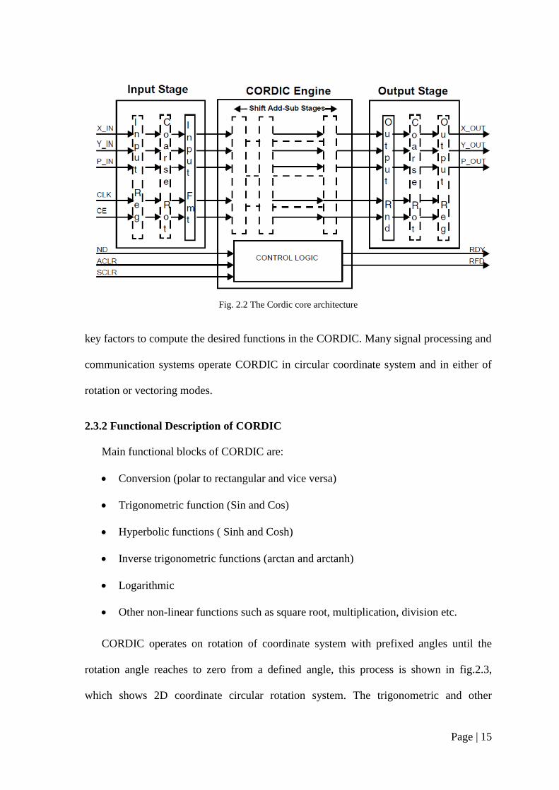
Fig. 2.2 The Cordic core architecture ................................................................................ 15

Fig. 2.3 2D circular rotation of a vector by an angle in coordinate system ....................... 16

Fig. 3.1 Proposed Method for Facial Expression Recognition System ............................. 21

Fig. 3.2 Process to find feature vector using Discriminating Feature Analysis ................ 24

Fig. 3.3 Detailed process of Face Detection ...................................................................... 27

Fig. 3.4. (a) Gabor wavelet, (b) an image and (c) convolved image with Gabor wavelet . 28

Fig. 4.1 Block diagram for Dimensionality Reduction process of Classification ............. 34

Fig. 4.2 Block diagram for mean calculation ..................................................................... 35

Fig. 4.3 Block diagram for Covariance module ................................................................ 35

Fig. 4.4 Block diagram for Eigen Loop ............................................................................ 36

Fig. 4.5 Block diagram for (cos α, sin α) module using CORDIC .................................... 37

Fig. 4.6 Block diagram for Arctan function using CORDIC ............................................ 37

Fig. 4.7 Block diagram for Principal component calculation ............................................ 38

Fig. 4.8 Delay path model for FPGA implementation ....................................................... 39

Fig. 5.1 Example of Variance face class images ............................................................... 42

Fig. 5.2 Example of Variance non-face class images ........................................................ 42

Fig.5.3 Example of images from JAFFE Database showing various emotions ................ 43

Fig. 5.4 Example of pre-processed images of JAFFE Database ........................................ 43

Fig. 5.5 Simulation waveform of FPGA implemented model ........................................... 45

Fig. 5.6 Chart comparing performance of proposed method with that of existing methods

................................................................................................................................... 47

vi

LIST OF TABLES

Table 4-1 Parameters for Gabor Wavelets generation ...................................................... 33

Table 5-1 Accuracy of Face Detection using Bayesian Discriminating Feature Analysis

Method .............................................................................................................. 43

Table 5-2 Percentage of Correct and Erroneous Emotion Recognition With Training

Database and Test Images from JAFFE Database ............................................ 44

Chapter 1

Introduction

Page | 2

Today, in a world of automation, human-computer interaction (HCI) is a wide

area of research and applications. As, human to human interpersonal communication can

be categorized in two types, verbal communication and non-verbal communication (facial

expressions, hand gestures and tone of the voice), where verbal communication is

essential yet non-verbal communication plays an important role where expression says a

lot more than words, similarly HCI can also be of above two types. Non-verbal

communication is backbone of HCI. For HCI, there are two major constraints, first

understanding Facial expression and second understanding Hand/arm movement (gesture)

[17]. Tactlessly, presently available human–computer interfaces systems are not

providing full benefit of these valuable communicative media, thus unable to deliver the

advantages of natural interaction to the users. HCI can be more useful if computers can

understand facial expression of the user and then act according to the recognized emotion

of the user.

The first constraint of HCI is facial expression recognition as emotions are

unavoidable part of communication even if we talk of verbal communication. In day to

day life, human show many expressions which are outcome of ones‟ internal state or

psychological state, which is response to the events occurring in the surroundings and

these expressions form emotions. The movement of main organs of the face such as

opening of mouth, widening of eyes, narrowing or frowning of eyebrows and cheek

movements play main role in forming and expressing emotions. On the basis of

appearance and movements of face organ only human do recognise others‟ emotions, so

the HCI system has to develop which sense the changes and movements in face organs

while communication and result in recognised emotions. To make a facial expression

recognition system fruitful, fast and accurate response of system are key parameters,

Page | 3

failing which results produced may not be useful or turn to be confusing at times,

depending on the application of system [1−4].

1.1 Types of Emotion

There are a number of micro facial expression which human expresses such as

affection, anger, angst, annoyance, anguish, anxiety, apathy, awe, arousal, boldness,

boredom, contentment, curiosity, contempt, depression, desire, disappointment, despair,

disgust, dread, embarrassment, envy, ecstasy, euphoria, excitement, fearlessness, fear,

frustration, gratitude, guilt, grief, happiness, hatred, horror, hope, hostility, hysteria, hurt,

indifference, interest, joy, jealousy, loathing, loneliness, lust, love, misery, nervousness,

passion, panic, pity, pride, pleasure, rage, regret, sadness, remorse, satisfaction, shame,

shyness, shock, sorrow, suffering, terror, uneasiness, worry, wonder, zeal, zest [13].

For HCI, it is not possible to detect each and every micro facial expression so

widely facial expression can be categories in basic seven categories namely anger,

disgust, fear, happy, sad, surprise and neutral [1].

1.2 Applications of Facial Emotion Recognition System

Application of Facial emotion recognition can be seen in different HCI areas such as:

1. To aid autistic children

2. Robot control

3. Driver state surveillance

4. Computerized psychological counselling and therapy

5. In the detection of criminal and antisocial motives

Page | 4

Autistic children are found with a disorder known as, Asperger‟s Syndrome, an

autism spectrum disease, due to which autistic children are often face problem to

communicate with other people, in verbal mode [1]. As they are unable to understand

verbal communication, to read people‟s behaviour and talks, autistic children need to be

trained with non-verbal communication and facial expressions being an important cue of

interaction, they must learn to read emotions. Thus, for such children, an automatic real

time facial expression recognition system can be a boon during face to face interaction or

even to meet their daily communication needs.

1.3 Motivation

Facial expressions are identified by position and movement of face organs such as

eyes, cheeks, mouth. Thus facial expression representation is very sensitive to even slight

change in face organ location or movement. The process of emotion recognition includes

feature extraction and classification of extracted feature. Thus even small change in any

of the face organ leads to change in emotion and also extracted feature is changed. Now,

classifier should be efficient enough to monitor change in feature and map the feature to

correct emotion class. There are methods available for robust feature extraction based on

PCA [1], LDA [14], LBP [15], harr features [7], and more. For classification broadly used

is SVM [16] because of its accuracy but at the cost of complexity and more hardware

utilization. Other is based on Euclidean distance method which is less complex but shows

poor results too [18]. Thus facial expression recognition system suffers either with

accuracy or complexity in multi class classification part on hardware implementation.

Page | 5

1.4 Problem Description

Thus, the challenge is to design a classifier for multi-class classification which is

less complex, very accurate and feasible for hardware implementation along with to be

compatible with flow of process of facial expression recognition process.

1.5 Organization of Thesis

The thesis is organized as follows:

Chapter 2 describes the basic process of facial expression recognition, different

methods used in literature for different modules of whole emotion recognition

procedure, such as pre-processing, feature extraction and classification, have been

described briefly with comparison of pros and cons of each process. Also

introduction to CORDIC is given in this chapter.

Chapter 3 describes a proposed method for facial expression recognition system

with detailed process of face detection based on Bayesian discriminating feature

analysis, feature extraction using Gabor filters, PCA and proposed Extended

Bayesian method for classification.

Chapter 4 describes about implementation constraints which have been taken into

account while implementing the proposed work. Also VHDL implementation

process and its modules for classification process using CORDIC have been

shown.

Chapter 5 shows results of facial expression recognition process using proposed

work and compares the result with highly accurate existing models.

Chapter 6 concludes the work done with an insight into future scope of the work.

Chapter 2

Background

Page | 7

2.1 Facial Expression Recognition Process

Facial expression recognition process starts with capturing of image of desired

person whom emotion has to recognize. After this, two major processes are to be

followed, [5]:

Face Detection

Emotion Detection

Facial Expression recognition process is training based process where first some

image database is developed for both face detection (having two class types, face class

image and non-face class images) and emotion detection (containing images from all

seven emotion classes, anger, disgust, fear, happy, neutral, sad and surprize). Training

images are featured then on the basis of their property test image is featured and

classified. A generalized process for both face detection and emotion detection is shown

in Error! Reference source not found..

Fig. 2.1 Generalized process of face detection and emotion detection

Before applying images directly for emotion recognition process, unwanted area

and noise of the image should be removed so that extracted features only have required

and important values to make features robust. This purpose is solved by face detection

which gives only effective part of face removing all other unnecessary things. After face

detection comes the emotion detection part.

Pre-processing Feature

Extraction Classification

Testing Images

Recognized

Emotion

Training Images Training Images

Page | 8

There are numerous methods existing in literature which are widely used for pre-

processing, feature extraction and classification, some of them which gives high accuracy

results are described next in this section.

2.2 Methods Used for Different Modules of Recognition Process

2.2.1 Pre-processing methods

When it comes to face detection system, pre-processing of an image includes the

resizing, sharpening of face and non-face class images. When it comes to emotion

detection, pre-processing of image means to find effective area of face contributing for

feature extraction by removing background and lower face portion of body (if present).

There are many methods which have been approached for face detection as face detection

is being the first step of process in many applications like automatic face recognition,

human computer interaction (for expression recognition, emotional state recognition),

surveillance system etc. But emotion detection is an emerging topic of concern on which

less effective work is done, especially when it comes to considering real time hardware

implementation and it includes face detection as pre-processing step.

Some of the widely used methods for face detection are penned below along with

their pros and cons in view of our requirement constraints.

Skin Color Based Face Detection Algorithm

In [19], Sanjay Kr. Singh et al. presents an algorithm for face detection based on

skin colour. Colour is one of the important features of human faces n which basis

probability of face presence can be estimated. Using human skin colour as a tool for

feature for locating face in an image many advantages than other face detection methods

among which most important is speed of operation and definitely colour processing is

Page | 9

faster than any other kind of feature processing and this procedure becomes easier with

the fact that colour orientation is invariant under certain lighting conditions. The coloured

image under test is converted to all three colour space representation namely RGB,

YCbCr and HCI and algorithms based on these three colour spaces are combined together

to get a new skin colour based face detection to take the algorithm.

This method shows poor result as skin colour features are subject to change with

various lightening conditions with movement of objects. Even different camera produces

different colour ranges for the same person and time. Moreover this method does not

work for gray-scale images.

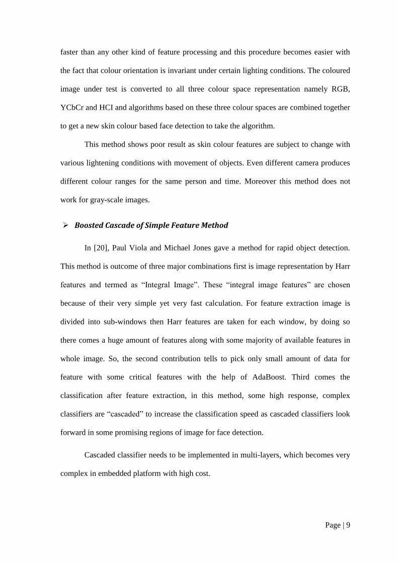
Boosted Cascade of Simple Feature Method

In [20], Paul Viola and Michael Jones gave a method for rapid object detection.

This method is outcome of three major combinations first is image representation by Harr

features and termed as “Integral Image”. These “integral image features” are chosen

because of their very simple yet very fast calculation. For feature extraction image is

divided into sub-windows then Harr features are taken for each window, by doing so

there comes a huge amount of features along with some majority of available features in

whole image. So, the second contribution tells to pick only small amount of data for

feature with some critical features with the help of AdaBoost. Third comes the

classification after feature extraction, in this method, some high response, complex

classifiers are “cascaded” to increase the classification speed as cascaded classifiers look

forward in some promising regions of image for face detection.

Cascaded classifier needs to be implemented in multi-layers, which becomes very

complex in embedded platform with high cost.

Page | 10

Bayesian Discriminating Feature Analysis Method

In [7], Chengjun Liu gave this method for face detection which uses Harr like

features for feature extraction but uses “difference images” unlike the previous discussed

method. Along with “difference images”, amplitude projections of image and image

pixels itself are combined to get robust features. For classification, this method uses

statistical modelling, PCA, conditional density function and Bayes classifier. Ease of

implementation with superb accuracy makes me to choose this in the project. Thus, the

method is discussed in section 3.2.

2.2.2 Feature extraction Methods

For emotion recognition second step is to extract facial feature out of the face

image and then to classify feature for emotion. Mainly two types of approaches are

reported to extract facial features (for both face detection and emotion detection), namely,

appearance-based methods and geometry-based methods. In geometric based feature

extraction process, the shape, movement and location of various face organs like

frowning of eyebrows, uplifting of cheeks, widening of eyes, are taken into consideration

for feature extraction and for this they require accurate and reliable facial organ

movement description, which is quite complex to achieve implement real time

applications in hard based systems. While, in the process of appearance-based feature

extraction [1], appearance changes in image are captured by applying them on image

filters.

Geometric feature extraction system gives robust features but proofs to be very

complex when it comes to real time hardware implementation while appearance based

method is easy to implement with high accuracy. So while keeping hardware constraints

Page | 11

in mind, we will focus on appearance based methods for pre-processing (face detection)

and emotion detection. Some of the techniques used for appearance based method are:

LDA (Linear Discriminant Analysis)

LBP (Local Binary Pattern)

PCA (Principal Component Analysis)

Harr-like Features method

Filter/ Kernel based methods

LDA Based Method

In [14], A. Djeradi et al. used a feature sub-space known as “fisher-space” to

project images. This projection reduces the dimensionality of the data matrix while

preserving the unique feature set. Training images are projected to this “fisher-space” for

feature extraction then test images are projected to LDA training space. Class information

extracted from fisher space is used to find unique vector set which minimizing the intra-

class scatters while maximizing the inter-class scatter.

Classification accuracy of LDA based method is affected by the "small sample

size" (SSS) problem.

LBP Based Method

In [15], Caifeng Shan et al. studied a method for face detection based on facial

local statical features which was earlier done for texture recognition. In this method

feature is extracted by considering 3×3 neighbour pixel of each pixel and then taking

threshold value of each neighbouring pixel with respect to centre pixel, formulating a

binary number belonging that block and finally take a 256 bit bin histogram as feature

descriptor.

Page | 12

Small neighbouring size loses some dominant features when applied on large

scale images which limit its effectiveness of operation.

PCA Based Method

Similar to LDA method, this PCA method uses “Eigen-space” for dimensionality

reduction and feature extraction. It uses eigen values and eigen vectors of the input data

matrix for calculation of principal component and later some significant principal

components are taken as feature descriptor. This method suffers from loss of data due to

dimensionality reduction and feature extraction can‟t bear data loss which makes it yield

less accurate result along with implementation ease [1].

Harr-like Features Method

Harr-features provides a promising feature extraction method by taking sub-

portion of image and calculating “integral images” or “difference images”. This method

provides very robust features but with repetition of features as integral or difference

images are linked to forth and back window of image. The robustness comes with

redundant data. The process is shown in [7] and [18].

Filter/Kernel Based Method

A kernel or filter bank is created with varying parameters and image under test is

convolved with the filter bank to map its feature with kernel. Such an approach is shown

in by Vitomir Struc and Nikola Pavesi C. in [11] which makes Gabor filter bank varying

with orientation and frequencies and image is mapped to this kernel. It provides

flexibility to choose size and robustness of feature by limiting number of scale and

orientation variation. This property is taken into advantage of this project and detailed in

section 3.3.1.

Page | 13

2.2.3 Classification Methods

Support Vector Machine (SVM)

SVMs are based on supervised learning methods, first model learns with the help

of training then perform pattern recognition on test images. SVM is a non-probabilistic

binary classification method where classes are separated by boundary and patterns are

shown as points in space. Binary SVM can be extended to multi-class but high degree of

complexity as shown in [16]. Above methods result best with SVM (support vector

machine) classification but SVM makes it complex to be implemented on embedded

platform hardware especially when it comes to multi-class classification.

KNN Classifier

KNN classifier as shown in [18], is based on Euclidean distance. Point to point

space distance is calculated from training to testing feature and the minimum is distance,

maximum is the similarity. This is the very basic and simplest method to classification

but suffers inaccuracy due to no cross point measures.

Bayes Classifier

Bayes classifier is for binary class classification, uses statistical model for

measuring parameter by calculating likelihoods of test image with classes [7]. The

accuracy and simplicity of implementation makes it useful for face detection which needs

binary class classifier and so detailed in section 3.2.

Page | 14

2.3 CORDIC and Its Applications

Many DSP and pattern recognition algorithms use elementary functions like

logarithmic, trigonometric, hyperbolic, exponential, division and multiplication. There are

two ways of implementing these functions, first by using lookup table method and second

is through polynomial expansions. The above mentioned methods require large number of

multiplications/divisions and additions/subtractions. Hardware implementation is done in

embedded platform environment which uses development boards such as Spartan, Virtex

etc. These are bounded by number of input-output pins, area, slices, flip-flops and

multiplication/division uses further excess adders/subtracts which is not feasible as it

crosses the source limitations.

2.3.1 What is CORDIC?

COordinate Rotation DIgital Computer (CORDIC) is a special purpose computer

useful to compute many non-linear and transcendental functions, was proposed by Volder

in 1959 and generalized by Walther later [22]. It is useful when there is no hardware

multiplier are provided and computation is done on additions/subtractions only. The

CORDIC core architecture is shown in fig 2.2, where all trigonometric, logarithmic and

other non-linear functions are computed using only shifts, additions and subtractions. The

functions that can be computed using a CORDIC computer include trigonometric,

logarithmic, exponential, hyperbolic, multiplication, division, square root, etc. [22].

Though it initially served the purpose of navigation systems, it later became a

popular tool to implement several digital systems especially in the areas of digital signal

processing, communications, computer graphics, etc. The simplicity of CORDIC is that it

can compute any of the above mentioned functions using shifts and additions which are

of the form (x± ). The operating mode and the coordinate system chosen are two

Page | 15

Fig. 2.2 The Cordic core architecture

key factors to compute the desired functions in the CORDIC. Many signal processing and

communication systems operate CORDIC in circular coordinate system and in either of

rotation or vectoring modes.

2.3.2 Functional Description of CORDIC

Main functional blocks of CORDIC are:

Conversion (polar to rectangular and vice versa)

Trigonometric function (Sin and Cos)

Hyperbolic functions ( Sinh and Cosh)

Inverse trigonometric functions (arctan and arctanh)

Logarithmic

Other non-linear functions such as square root, multiplication, division etc.

CORDIC operates on rotation of coordinate system with prefixed angles until the

rotation angle reaches to zero from a defined angle, this process is shown in fig.2.3,

which shows 2D coordinate circular rotation system. The trigonometric and other

Page | 16

arithmetic functions are executed by solving eqs.(2.3.1) with some predefined set of

conditions. In equations Xnew, Ynew are new coordinate value of Xold , Yold vectors after

rotating with angle ϴ.

Fig. 2.3 2D circular rotation of a vector by an angle in coordinate system

(2.3.1)

K is invariable constant in above equations.

Input/Output Data Representation

Fig 2.3 shows CORDIC core block where X_IN, Y_IN are input data signals and

X_OUT, Y_OUT are output data signals while p_in and p_out denotes phase input and

output signals. Clk, ce, ND, ACLR, SCLR are input control signals with two output

signals RFD and RDY. There is separate format for reading data signals and phase

signals.

Page | 17

XQN Number Format

This number format is used to represent signed values in 2‟s complement format.

This format is described as XQN => 1 sign bit + X bits for integer + N bits for

mantissa (fraction). So if „w‟ is word width then N = w − (X+1) bits will represent

fractional part of the value. This is also represented as Fix (N+X+1)_N using

system generator fixed format.

Data Signal Representation

o Input data signals (signed) should lie in the range from -1 to +1, outside

which CORDIC core gives unpredictable results. So to present maximum

integer of value „1‟ one bit is required with an additional bit for sign

representation. Thus input data signals are represented in 1QN format

where N= word_width – 2. It can also be represented as Fix(N+2)_N

format.

Example: If word width is 10bit then signed data signal will be

represented by 1Q8 format.

“0011000000” => 00.11000000 => +0.75

“1101000000” => 11.01000000 => −0.75

o When data signal set to unsigned fraction, value can be ranged 0 <= X_in

< +2 and integer is represented by 1 bit allowing it to represent as

UFix(N+1)_N format. N = word_width – 1.

Example:

“0011000000” => 0.011000000 => 0.375

o For unsigned integer, data signal range varies from 0 <= X_IN < 2**Input

Width.

Page | 18

Example:

“0011000000” => 192

Phase Signal Representation

Input phase signals (signed) should lay in the range from −∏ to +∏,

outside which CORDIC core gives unpredictable results. So to present maximum

integer of value „3‟, two integer bits are required with an additional bit for sign

representation. Thus input phase signals are represented in 2QN format where N=

(word_width – 3). It can also be represented as Fix(N+3)_N format. Phase is

represented in radians in CORDIC core.

Example: If word width is 10bit then phase signal will be represented by 2Q7

format.

“0011000000” => 001.1000000 => +1.5 radians

“1101000000” => 110.1000000 => −1.5 radians

2.3.3 Applications

CORDIC applications are mainly figured in following areas of development:

Matrix decomposition

Image processing

Digital signal processing

Communications implementations

Computer graphics

Robotics and many more.

With the base of this literature review and defined processes, further work is done.

Chapter 3

Proposed Algorithm for Facial

Expression Recognition

Page | 20

3.1 Overview

Facial expression recognition system has been designed by following the

procedure as shown in section 2.1 and the flow of proposed method is shown in fig 3.1. A

set of database containing numerous images showing all seven basic facial expressions

(anger, disgust, fear, happy, neutral, sad and surprize), with equal prior probabilities, is

taken and used for training of the system. All the training images are first pre-processed

to find the effective face area out of the image, which is useful for feature extraction. Also

the test image is pre-processed before it is used for future feature extraction and

classification. A pre-existing Bayesian discriminating feature analysis method [7], is used

for pre-processing, which is described in detail in section 3.2. This particular method is

used for pre-processing because of its simple implementation and robust and speedy

classification and as here classification is only between two classes, face class which

contains effective face portion of the human reducing all other noises and other is non-

face class which includes images from rest of the world, binary based Bayesian

classification shows the best result.

After pre-processing of training images, images belonging to same emotion class

are grouped together and combining features of each image of same emotion group, class

feature is generated which collectively represents an emotion feature. Since emotions are

represented by very minute details of face organs digitally, it becomes necessary to

extract very robust features for accurate classification which contains various aspects of

face appearance. To cover maximum available features Gabor filters, its wavelets and

generated features are used for feature extraction and described in section 3.2 in detail

[11]. Since Gabor wavelets can be generated depends on various frequencies and scales,

higher the frequency and scale, robust will be the feature with hardware cost. So there

Page | 21

comes a trade-off between feature robustness and hardware cost and one can choose

depending on high priority. Test image features are is also extracted using this method.

Fig. 3.1 Proposed Method for Facial Expression Recognition System

As Gabor features are of very high dimensionality, to reduce its computational

complexity PCA is used. By calculating eigen values and eigen vectors of feature matrix,

principal components of the feature vector is estimated. Section 3.3 shows how PCA is

used for dimensionality reduction.

Reduced dimensionality class features are modelled with test image feature. Here

modelling means to estimate the similarity between class feature and test image feature

and classification is based on measure of similarity. For this conditional density function

is used with its logarithm value, it shows the likelihood amount of one category to other,

shown in section 3.4.1. Since here multi-class classification is required an Extended

Bayes classifier is proposed contrary to binary Bayes classifier, detailed in section 3.4.2.

Extended Bayes classifier gives very high accuracy rate and is far easier for embedded

platform implementation as compared to support vector machine (SVM) which is widely

used for classification but loses implement ability for multi class classification.

Page | 22

3.2 Pre-processing

An image or portion of image (window) may belong to face class or non-face

class (rest of the world). To identify face in an image, we check in window in varying

size of image whether that particular portion belongs to face class or non-face class. For

this, training is done with both face class images and non-face class images. For window

under test of test image, discriminating feature vector for feature extraction is applied

then log likelihood of conditional density function of extracted feature with respect to

both face class and non-face class is calculated and to identify to whether there is face or

not, Bayes classification rule is applied on calculated log likelihood.

3.2.1 Discriminating Feature Analysis

An enhanced and simple feature is estimated in discriminating feature analysis by

combining Harr features and amplitude projections to give high discriminating power of

features [7], graphically shown in fig.3.2. If image A(i,j) ∈ Rm × n

then discriminating

feature vector of image, Y, is calculated by combining :

a) Image A

b) 1D Harr representation of image A

c) Amplitude projection of image A

1D Harr representation includes calculation of horizontal difference image and

vertical difference image of image A(i, j), Ah(i, j) ∈ R(m-1) x n

and Av(i, j) ∈ Rm× (n-1)

respectively.

Ah(i, j) = A(i+1,j) – A(i, j) 1≤ i <m, 1≤ j ≤n (3.2.1)

Av(i, j) = A(i,j+1) – A(i, j) 1≤ i ≤m, 1≤ j<n (3.2.2)

Page | 23

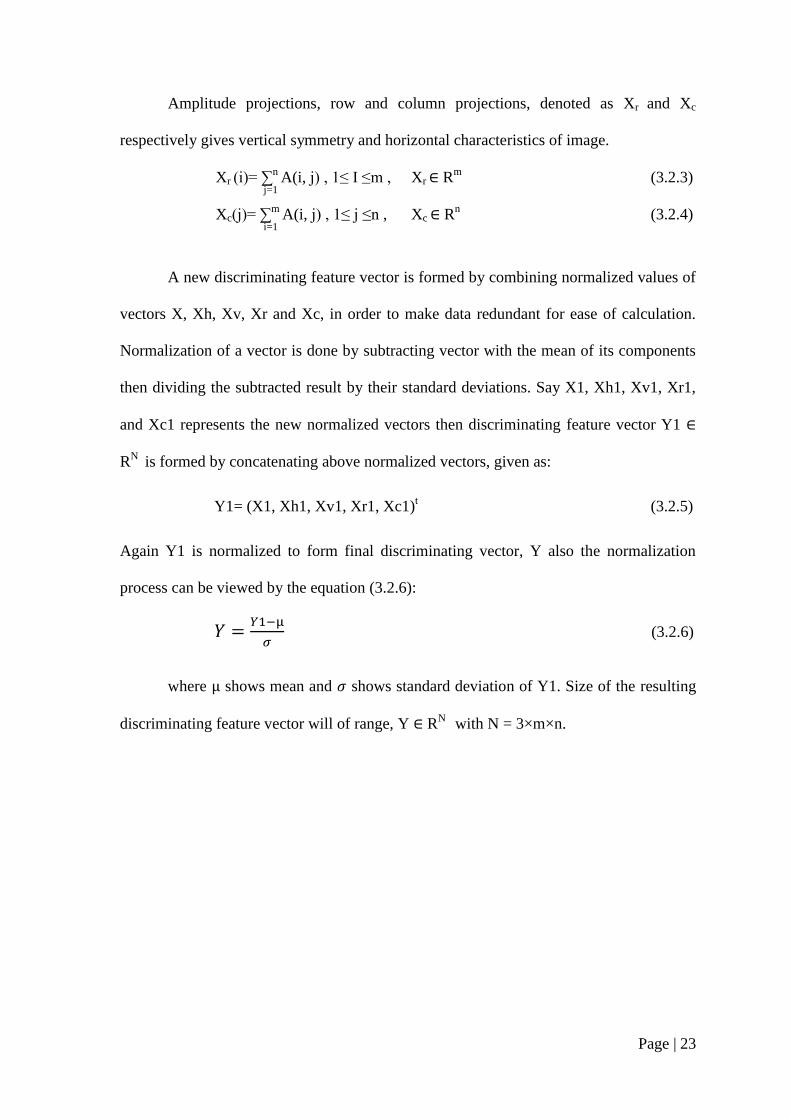
Amplitude projections, row and column projections, denoted as Xr and Xc

respectively gives vertical symmetry and horizontal characteristics of image.

Xr (i)= ∑n

A(i, j) , 1≤ I ≤m , Xr ∈ Rm

(3.2.3)

j=1

Xc(j)= ∑m

A(i, j) , 1≤ j ≤n , Xc ∈ Rn (3.2.4)

i=1

A new discriminating feature vector is formed by combining normalized values of

vectors X, Xh, Xv, Xr and Xc, in order to make data redundant for ease of calculation.

Normalization of a vector is done by subtracting vector with the mean of its components

then dividing the subtracted result by their standard deviations. Say X1, Xh1, Xv1, Xr1,

and Xc1 represents the new normalized vectors then discriminating feature vector Y1 ∈

RN

is formed by concatenating above normalized vectors, given as:

Y1= (X1, Xh1, Xv1, Xr1, Xc1)t

(3.2.5)

Again Y1 is normalized to form final discriminating vector, Y also the normalization

process can be viewed by the equation (3.2.6):

(3.2.6)

where shows mean and shows standard deviation of Y1. Size of the resulting

discriminating feature vector will of range, Y ∈ RN

with N = 3×m×n.

Page | 24

Fig. 3.2 Process to find feature vector using Discriminating Feature Analysis

Page | 25

3.2.2 Statistical Modelling

Statistical modelling estimates the conditional probability density functions, of

any class for test image using multivariate normal distribution will be used later for

classification for feature.

Let w is feature matrix representing particular class, M is mean of class feature

(w) and ∑ is covariance matrix then multivariate normal distribution of w is represented

as

w = N(M, ∑) (3.2.7)

Since, multivariate normal distribution is of high dimensionality so to make it ease

with computation, an important property, optimal signal reconstruction, of principal

component analysis (PCA) is used for dimensionality reduction. Only a part of original

signal can be used to represent the whole signal as, PCA uses minimum mean square

error for reconstruction of signal [6]. If eigen vector space and eigen values of covariance

matrix are denoted by ϕ and λ respectively and Y is test image feature vector then

principal component of deviation of test image with particular class can be calculated by

eq.(3.2.8)

Z= ϕt (Y -M) (3.2.8)

With the use of PCA above property, inspite of using all principal components,

only first Mn, (Mn << N) components are used to formulate the conditional density

function and impact of other principal components can be included by adopting

Moghaddam and Pentland model [21], that calculates eigen value equivalent for the rest

(N –Mn) eigen values, by the averaging them:

ρ =

∑ (3.2.9)

Page | 26

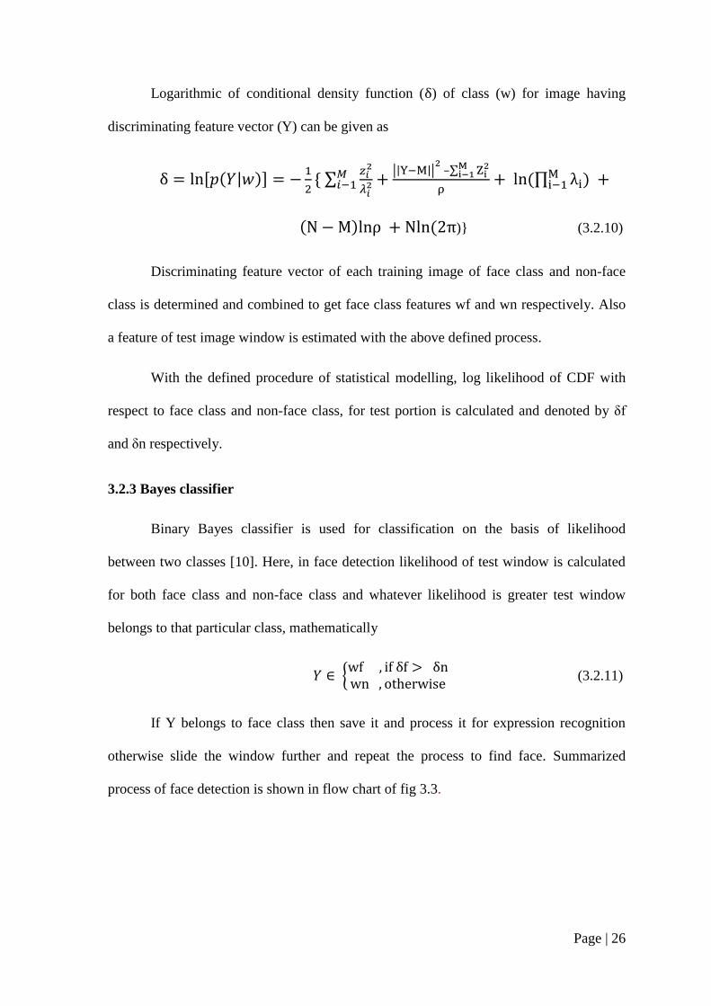
Logarithmic of conditional density function ( ) of class (w) for image having

discriminating feature vector (Y) can be given as

[ ( | )]

* ∑

|| || –∑

(∏ )

( ) ( )} (3.2.10)

Discriminating feature vector of each training image of face class and non-face

class is determined and combined to get face class features wf and wn respectively. Also

a feature of test image window is estimated with the above defined process.

With the defined procedure of statistical modelling, log likelihood of CDF with

respect to face class and non-face class, for test portion is calculated and denoted by δf

and δn respectively.

3.2.3 Bayes classifier

Binary Bayes classifier is used for classification on the basis of likelihood

between two classes [10]. Here, in face detection likelihood of test window is calculated

for both face class and non-face class and whatever likelihood is greater test window

belongs to that particular class, mathematically

∈ {

(3.2.11)

If Y belongs to face class then save it and process it for expression recognition

otherwise slide the window further and repeat the process to find face. Summarized

process of face detection is shown in flow chart of fig 3.3.

Page | 27

Fig. 3.3 Detailed process of Face Detection

Page | 28

3.3 Feature extraction using Gabor Wavelets

3.3.1 Gabor Wavelet Representation

For 2D data, Gabor wavelet is given by [11],

2 22 2

2 22

2( , , , )

cos sin

sin cos

t t

t

f fx y

j fx

t

t

ff e e

x x y

y x y

(3.3.1)

Here, f is sinusoidal frequency, θ is wavelet orientation, γ is the spatial width along the

sinusoidal plane wave, η represents spatial width of wavelet which is perpendicular to the

wave and x,y represents the coordinates of pixels. By varying the scale (f) and orientation

(θ), a filter bank is created. The scale and orientation are changed according to equations

given by eq. (3.3.2) :

max

,

/ 2 ,

,8

( , ) ( , , , )

g

g

h

g h g h

f f

h

x y f

(3.3.2)

The value of parameters in Eq.(2) are given by γ = η = 2 , fmax = 0.25 with g

{0,…,3}, h {0,…,7}, generally. In the current work both scale and orientation are taken

as (g,h) {0,…,7}, to extract more discriminating features.

(a) (b) (c)

Fig. 3.4. (a) Gabor wavelet, (b) an image and (c) convolved image with Gabor wavelet

Page | 29

3.3.2 Feature Extraction from Gabor Wavelets

Each component of the 2-D Gabor wavelet (at different scales with different

orientations) is convolved with image (A) and given by Eq. Down sampling is performed

by a factor of 4 in rows and columns of the absolute value of the filtered image. The

feature vector is obtained by rearranging the down sampled value.

, ,( , ) ( , ) ( , )g h g hO x y A x y x y (3.3.3)

The vector F, is normalized to have unit variance and zero mean. If og,h denotes the

feature vector from the filtered image at scale g and orientation h, then final feature (F)

value in Rd is given by Eq.(4)[11]. For m×n image, the size of feature space dimension,

d = m×n×g×h/(d1×d2) (3.3.4)

Where „g‟ is number of frequency scale and „h‟ is number of orientations taken into

account to create Gabor filter bank.

The feature extraction method is performed using a Gabor filter bank of scales and

orientations both equal to 8. The pixel coordinates x, y (in Eq.(1)) is taken as 39, 39 as in

[12], and the final feature vector is given by eq.(3.3.4).

3.4 Principal component analysis

PCA is used for dimensionality reduction as dimensionality reduction gives a

compact, effective and low-dimensional feature for a given high-dimensional data set. In

an N dimensional space, if PCA is applied then it aims to find a linear subspace with

lower dimensionality say D where (D << N) while maintaining almost all variability of N

dimensional data. Eq.(3.4.1)-(3.4.5) shows the how to calculate the principal components

using eigen values and eigen vectors. First D principal components, associated with D

largest eigen values are considered to represent reduced dimensionality vector [1].

Page | 30

Let Ai is featuring vector of an image after feature extraction using Gabor

wavelets. All the feature vectors of image belonging to same emotion class are grouped

together to form class feature matrix. Let say „A‟ represents class feature matrix then

process to calculate principal components of it is as follows:

A = [A1, A2, A3……… An] (3.4.1)

where „i‟ is number of images belonging to same class. Mean (An,mean) of all „n‟

images is calculated and deviation of image by mean is calculated and represented by Ã.

Ãn = An – An,mean (3.4.2)

To find principal component of a matrix its eigen values and eigen vectors are

required and for this Covariance matrix is used because use of its symmetry property

makes calculation overhead half of the actual. Let „cov‟ represents covariance matrix of A

then it can be calculated as;

∑ (

)

(3.4.3)

Covariance matrix „cov‟ comes out to be a n×n matrix. The process of finding

eigen values and eigen vectors of this matrix is by Jacobi Algorithm, as follows:

Step 1.Start with an identity matrix U and covariance matrix cov.

Step 2.Find out the off diagonal element with largest absolute value, covij then take out

corresponding diagonal elements covii and covjj using to calculate rotation angle „α’ using

eq.(3.4.4),

(

) (3.4.4)

Step 3.Take an identity matrix V except for Vii = Vjj = cos α, Vji = -sin α, and Vij = sin α.

Page | 31

Step 4.Compute the matric products C′′ and U′′ such that C′′ij becomes zero and other

elements of matrix changes.

C′′ = V′×cov×V and U′′ = U×V (3.4.5)

Step 5.Compare maximum absolute value of off diagonal element (covij) with threshold

value, if covij is greater repeat steps from step 2 to step 5 until convergence with C′′ as cov

and U′′ as U. Upon convergence C′′ diagonal elements contains eigen values and U′′

contains eigen vectors. U′′ and C′′ both are of size n×n.

Eigen vector associated with highest eigen value gives principal component and

so on effectiveness of components decreases with decreasing eigen values. If X is (m×n)

size data which is projected to eigen space Z = XU′′, principal components are in order of

U′′.

3.5 Extended Bayesian classifier for classification

3.5.1 Modelling

Feature vector of training images, belonging to same emotion class, is estimated

using eqs.(3.3.1)– (3.3.4), and are grouped together to form particular class feature vector.

If emotions are categorized in „C‟ number of classes, class feature vectors, wk, for each

class (k=1 to C) are obtained to get covariance matrix of size (d×d), where d is given in

eq(3.3.4). These covariance matrix features are undergo dimensionality reduction by

using PCA. For PCA, eigen values and eigen vectors of covariance matrix are calculated

and PCA is applied as shown in section 3.2.2. Similarly feature vector (Y) of test image is

estimated using eqs.(3.3.1)– (3.3.4) . Conditional density function and its logarithm using

PCA is shown in eq.(3.5.1)-(3.5.2) below [7],

( | )

( ) |∑| {

( ) ∑

( )} (3.5.1)

Page | 32

[ ( | )]

* ∑

|| || –∑

(∏ )

( ) ( ) } (3.5.2)

where M and ∑ are mean and covariance of class feature vector „w‟ and „L‟ shows

likelihood of test image with respect to class w.

3.5.2 Classification

If there are „k‟ number of classes (k = 1 to C) then for each „k‟ emotion class (k =

1 to C), likelihood of test image „Lk‟ is estimated using eq.(3.5.3). To classify the

estimated likelihoods, Lk, (k = 1 to C), proposed method extends the binary Bayes

classifier to multi-class classifier (having equal class priors), such that class „k‟ having

the maximum value of logarithmic of conditional density function, shows maximum

similarity of that class feature to test image feature thus test image is categorized under

„k‟th

emotion class, mathematical shown in eq.(3.5.3)

1

(L )

observed kk C

C argmax (3.5.3)

Eq.(9) recognizes the emotion class „Cobserved’ as the emotion label of the test

image. Prior probabilities of each emotion class are equal, as equal number of training

images in each class has been taken.

This proposed method has been implemented and tested in the subsequent

sections.

Chapter 4

Implementation

Page | 33

4.1 MATLAB Implementation

The proposed method is implemented following the process described in chapter

3. The pre-processing of images is done by Bayesian discriminating feature analysis

method with (M = 10) principal components taking into account for modelling by using

eqs. (3.2.1) to (3.2.11) using MATLAB.

Pre-processed images are undergoing for feature extraction as per section 3.3

using Gabor wavelets. Table 4-1 shows the parameters taken while designing Gabor

wavelets and also for feature extraction using wavelets. The features are extracted using

eqs. (3.3.1) to (3.3.3). Eq.(3.3.4) gives the size of the feature of an images. With the

defined parameters size of the feature comes out to be (1024×1) since (d =

16×16×8×8/(4×4) = 1024).

Table 4-1

Parameters for Gabor Wavelets generation

Gabor wavelets

No. Of frequencies (g) 8

Orientations (h) 8

No. of rows in 2-D Gabor filter 39

No. of columns in 2-D Gabor filter 39

Gabor features extraction

Factor of down sampling along rows (d1) 4

Factor of down sampling along columns (d2) 4

Each class feature is computed by combining similar class images. Since size of

the feature is very large, PCA is applied on class features using eqs.(3.4.1) to (3.4.5) for

dimensionality reduction and effective first 10 principal components (M=10), are

considered for modelling using eqs.(3.5.1) and (3.5.2) and likelihood is calculated for

each training class, anger, disgust, fear, happy, sad, surprize and neutral. Now calculated

Page | 34

likelihoods for each class are compared with each other to find which class shares

maximum similarity with the test image and the class with max likelihood is recognized

as recognized emotion class for given test image.

4.2 FPGA Implementation of Post Feature Extraction Process

After pre-processing and feature extraction of using MATLAB, the

dimensionality reduction and modelling part is implemented in FPGA using Xilinx 10.1.

The computational block diagram which is designed by following Jacobi Algorithm, as in

section 3.4, is shown in fig. 4.1.

Fig. 4.1 Block diagram for Dimensionality Reduction process of Classification

Let say „A‟ is feature matrix of representing any class and Y is feature of test

image after Gabor feature extraction. Since class feature is accumulation of various

images, covariance of class feature is calculated to take the measure of difference among

images. Covariance is a symmetric matrix where diagonal elements shows variance of an

image with its different components while off diagonal elements shows difference

between different images. Taking advantage of symmetry property of covariance matrix,

while calculation; only upper triangular off-diagonal elements are calculated and lower

half are assigned copying the upper triangular elements, it saves hardware utilization.

Page | 35

Covariance is calculated using eq.(3.4.3) where deviation of feature (A1), with its

mean (Amean), is need to be calculated. The mean is calculated as shown in fig. 4.2. If

each column represents an image in class then column wise mean is calculated and

subtracted with its respective column to find deviation. Since feature is of (1024×1) size,

division operation for mean is calculated using right shift property of HDL, and to divide

by 1024 times, vector is right shifted 10 bits (1024 = 210

). Deviation A1 and its transpose

A1‟ are calculated and fed to Covariance block, fig. 4.3, which calculates upper triangular

elements by adding and multiplying elements logically then divided by using CORDIC

divider.

Fig. 4.2 Block diagram for mean calculation

Fig. 4.3 Block diagram for Covariance module

As per the steps of Jacobi Algorithm of section 3.4, eigen values and eigen

vectors are calculated iteratively using covariance matrix cov, With covariance block an

identity matrix U is also formed. Using Eigen loop block, fig. 4.4, each iterative value of

C2 and U2 is calculated until threshold is reached. Here in this particular implementation

Page | 36

threshold is set to „2‟. Mux is used in top block, fig.4.1 to make iterations according to

threshold. Max value and indices block calculates max value among absolute values of

off-diagonal elements of C1, along with the indices, max value index and its symmetric

part index (max_index and symm_max_index), its corresponding diagonal elements

index (diag_i and diag_j) are calculated. (Cos α, sin α) block is implemented to fulfil

steps 3 followed by matrix V and (C2,U2) block of step 4. Threshold comparator of fig.

4.1, compares the max_element and threshold, which is set to „2‟ to generate a flag of

condition satisfaction, and this flag works as select line for mux.

Fig. 4.4 Block diagram for Eigen Loop

Fig. 4.5 shows implementation of block used to generate cos α and sin α signals.

Alpha angle is calculated using eq.(3.4.4) which uses tan inverse function. Tan inverse

function and cos and sin functions are implemented using CORDIC ip core 4.0. The

CORDIC cos, sin values are read using XQN format as described in section 2.3.2.

Page | 37

Fig. 4.5 Block diagram for (cos α, sin α) module using CORDIC

To implement tan inverse function there is an arctan function available in

CORDIC but that gives phase angle correctly when values of tangents (X and Y) are

subjected to first quadrant (i.e. both positive) only, otherwise it gives garbage as its output

phase limitation is upto (-pi/4 to +pi/4). So to realize an arctan function which is suitable

for all four quadrants some functionality has to be added with CORDIC block as shown

in fig. 4.6. As we know, if phase_out is tan inverse angle when tangents lie in first

quadrant then angle for rest quadrants can be calculated as :

sel => 00 => angle <= phase_out (Ist quadrant)

sel => 10 => angle <= pi - phase_out (IInd

quadrant)

sel => 01 => angle <= − (phase_out) (IIIrd

quadrant)

sel => 11 => angle <= − pi + phase_out (IVth

quadrant)

Fig. 4.6 Block diagram for Arctan function using CORDIC

Page | 38

In fig. 4.6, (magnitude and sign sel) block store the magnitudes and signs of inputs (X and

Y) and according to signs generates sel signal. On magnitude values tan inverse function

is operated and then according to sel signal angle is rotated using Phase rotation having

above functionality, which gives the correct tan inverse angle.

After calculating eigen values and eigen vectors from fig. 4.1 and intermediate

blocks, fig.4.7 shows the process of calculating principal components using eq. (3.2.8).

Fig. 4.7 Block diagram for Principal component calculation

Here first block selects the M principal components corresponding to M maximum

eigen values and gives eigen vector matrix Φ. Second block finds the deviated feature

matrix and fed to multiplier. Multiplier multiplies the transpose of matrix Φ and temp

matrix signal to generate principal components Z. These principal components are further

used in eq.(3.5.1) to (3.5.3) to model and classification.

Delay Path Model for FPGA Implementation

While designing for hardware implementation, one of the most important aspects

is the synchronization between different modules of design. Since clock is the measure of

latency in HDL design, inputs to particular module should reach at same time to avoid

cross calculation of data. To maintain the synchronization latencies if blocks are

calculated pre-hand and delay wherever required are given as shown in fig. 4.8.

Page | 39

Fig. 4.8 Delay path model for FPGA implementation

Page | 40

In flow graph, number with arrow shows the delay required to provide to input of

successive signal or block to maintain the synchronization in output of that particular

block, in such manner full design is synchronized. For an example, in the above design,

tan inverse function has latency of 14 clock cycles and further (sine, cosine) block has

latency of 20 clock cycle, since for calculation of matrix V output of (sine, cosine) block

and all the indices are required so to make these in sync, delay of 34 clock cycles (14 +

20 =34) is given to indices signals. In the similar way whole design is synchronized.

Chapter 5

Results and Analysis

Page | 42

5.1 Simulation Results

Both face detection and emotion detection processes are implemented using

constraints defined in chapter 4. Since both face detection and emotion detection are

supervised learning method, first system is modelled and trained using training images

(from both face-class and non-face class in case of face detection and images from all

seven emotion classes in case of emotion detection) then test images are subjected to the

system to be classified.

The pre-processing steps i.e. face detection method is implemented with (M=10)

principal components and trained using 2400 face class images and 4500 non-face class

images from variance face class database and variance non-face class database

respectively. Since non-face class images may contain images from rest of the world

except face image, so there is hell number of images belonging to this class but for

training, images with similar variance to face class are taken into account. The examples

of face class and non-face class variance images are shown in fig.(5.1) and fig.(5.2)

respectively.

Fig. 5.1 Example of Variance face class images

Fig. 5.2 Example of Variance non-face class images

Facial expression recognition algorithm is tested on JAFFE database so JAFFE

database is first pre-processed (face detection) then used in emotion recognition part for

both training and testing.

Page | 43

JAFFE Database: JAFFE is an acronym for Japanese Female Facial Expresion.

JAFFE database provides 213 images posed by 10 Japanese females showing all the

seven basic emotions (Anger, Disgust, Fear, Happy, Sad, Surprise and Neutral) [10].

The database was planned and assembled by Michael Lyons, Miyuki Kamachi, and

Jiro Gyoba. These images were taken when these females were subjected to sudden

feel of any of the above described emotions. The example of images from JAFFE

database is shown below in fig. 5.3.

Fig.5.3 Example of images from JAFFE Database showing various emotions

Images from JAFFE database have been pre-processed, the accuracy of pre-

processing and resized to 16×16 for training as well as testing has been shown in Table 5-

1below and fig.5.4 shows example of pre-processed images.

Table 5-1

Accuracy of Face Detection using Bayesian Discriminating Feature Analysis Method

Set Sources Number of

Images

Detected

face

Undetected

face

Accuracy

Set1 JAFFE Database 213 205 8 96.244%

Fig. 5.4 Example of pre-processed images of JAFFE Database

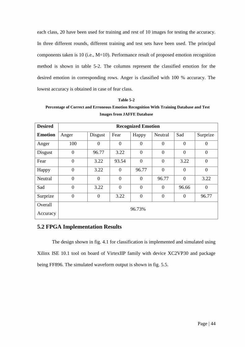
JAFFE database have 210 images of frontal face showing seven emotions posed

by 10 Japanese female models. Each emotion class has 30 images. Out of 30 images in

Page | 44

each class, 20 have been used for training and rest of 10 images for testing the accuracy.

In three different rounds, different training and test sets have been used. The principal

components taken is 10 (i.e., M=10). Performance result of proposed emotion recognition

method is shown in table 5-2. The columns represent the classified emotion for the

desired emotion in corresponding rows. Anger is classified with 100 % accuracy. The

lowest accuracy is obtained in case of fear class.

Table 5-2

Percentage of Correct and Erroneous Emotion Recognition With Training Database and Test

Images from JAFFE Database

Desired

Emotion

Recognized Emotion

Anger Disgust Fear Happy Neutral Sad Surprize

Anger 100 0 0 0 0 0 0

Disgust 0 96.77 3.22 0 0 0 0

Fear 0 3.22 93.54 0 0 3.22 0

Happy 0 3.22 0 96.77 0 0 0

Neutral 0 0 0 0 96.77 0 3.22

Sad 0 3.22 0 0 0 96.66 0

Surprize 0 0 3.22 0 0 0 96.77

Overall

Accuracy 96.73%

5.2 FPGA Implementation Results

The design shown in fig. 4.1 for classification is implemented and simulated using

Xilinx ISE 10.1 tool on board of VirtexIIP family with device XC2VP30 and package

being FF896. The simulated waveform output is shown in fig. 5.5.

Page | 45

Fig

. 5

.5 S

imula

tio

n w

avefo

rm o

f F

PG

A i

mp

lem

ente

d m

od

el

Page | 46

5.3 Comparison

The performance of proposed method is compared with existing highly accurate facial

emotion recognition models listed below and comparison chart is shown in fig.5.6.

The method proposed in [2], based on fuzzy relational approach shows overall 88.2 %

accuracy when tested on Set, containing images of 100 Indian male showing 6

emotions (except neutral). It shows 92.2 % accuracy when tested on Set2, contains

images of 100 Indian female showing 6 emotion (except neutral).

The method proposed in [4], which is based on facial movement analysis, shows

92.92 % accuracy when tested on Set1 containing 180 images from JAFFE database

showing 6 emotions (except neutral) and 93.14 % accuracy when tested on Set2,

containing 800 images from Cohn-Kanade database showing 6 emotions.

Method proposed in [5] based on local directional number pattern, shows 96.68 %

accuracy when tested on Set1, contains images from Cohn-Kanade database showing

all seven emotions.

In [6], 94 % accuracy is obtained by using Hidden Markov Model method for

recognition.

Facial action units based method in [8], which is, shows 87.43% accuracy when tested

on Set1, contains images from Cohn-Kanade database showing 6 emotions (except

neutral).

Page | 47

Fig. 5.6 Chart comparing performance of proposed method with that of existing methods

The comparison chart shows that the proposed method of facial expression

recognition has highest accuracy when tested on JAFFE database and anger emotion class

has 100 % accuracy, which is also highest among other methods.

6062646668707274767880828486889092949698

100Anger

Disgust

Fear

Happy

Sad

Surprize

Neutral

OverallAccuracy

Chapter 6

Conclusion

Page | 49

6.1 Conclusion

A method for facial emotion recognition based on Gabor wavelet based feature

and extended Bayesian classifier for multi class classification is proposed. The proposed

method shows overall accuracy of 96.73% for JAFFE database, when implemented on

MATLAB which is higher than that of highly accurate existing facial emotion recognition

methods. Also existing method for Face detection based on Bayesian discriminating

feature analysis is implemented successfully with accuracy of 98.59% when tested on

JAFFE database. The simple extended Bayesian classifier is suitable for real time

implementation and is implemented on FPGA VirtexIIpro using Xilinx ISE 10.1

simulator with CORDIC IP Core. The ease of implementation and hardware efficiency of

CORDIC IP core makes the FPGA implementation area efficient and faster. The

intellectual properties of CORDIC core have been used significantly for calculation of

logarithm, sin, cos, tan and arctan functions.

6.2 Scope for Future Work

To implement the remaining existing modules of feature extraction and face

detection in HDL and to perform full FPGA implementation of algorithm in

hardware.

Real time implementation of the proposed algorithm for facial expression

recognition.

Realization and implementation of second parameter of HCI that is gesture

recognition.

ASIC implementation for HCI including both emotion and gesture recognition.

Page | 50

BIBLIOGRAPHY

[1] K.G. Smitha and A.P. Vinod, “Hardware Efficient FPGA Implementation of

Emotion Recognizer for Autistic Children,” IEEE CONECCT, pp.1–4, 2013.

[2] A. Chakraborty and A. Konar, “Emotion Recognition from Facial Expressions and

its Control using Fuzzy Logic,” IEEE Transactions on Systems, Man and

Cybernetics- Part A: Systems and Humans, vol.39(4), pp.726–743, 2009.

[3] T. Senechal, V. Rapp, H. Salam, R. Seguier, K. Bailly and L. Prevost, “Facial

Action Recognition Combining Heterogeneous Features via Multikernel

Learning,” IEEE Transactions on Systems, Man and Cybernetics- Part B:

Cybernetics, vol.42(4), pp.993–1005, 2012.

[4] L. Zhang and D. Tjondronegoro, “Facial Expression Recognition Using Facial

Movement Features,” IEEE Transactions on Affective Computing, vol.2(4),

pp.219–229, 2011.

[5] A.R. Rivera, J.R. Castillo and O. Chae, “Local Directional Number Pattern for

Face Analysis:Face and Expression Recognition” IEEE Transactions on Image

Processing, vol.22(5), pp.1740–1752, 2013.

[6] M. Lahbiri et al., “Facial Emotion Recognition with the Hidden Markov Model,”

International Conference on Electrical Engineering and Software Applications

(ICEESA), pp.1–6, 2013.

[7] C. Liu, “A Bayesian Discriminating Features Method for Face Detection,” IEEE

Transactions on Pattern Analysis and Machine Intelligence, vol.25(6), pp.725–

740, 2003.

[8] Y. Li, S. Wang, Y. Zhao and Q. Ji, “Simultaneous Facial Feature Tracking and

Facial Expression Recognition,” IEEE Transactions on Image Processing,

vol.22(7), pp.2559–2573, 2013.

Page | 51

[9] G. Littlewort, M.S. Bartlett, I. Fasel, J. Susskind and J.R. Movellan, “Dynamics of

Facial Expression Extracted Automatically from Video,” Image and Vision

Computing, vol.24, pp.615–625, 2006.

[10] M. Lyons, M. Kamachi and J. Gyoba. (1998, April). The Japanese Female Facial

Expression (JAFFE) Database. [Online]. Available:

http://www.kasrl.org/jaffe.html

[11] V. Struc and N. Pavesic, “Gabor-Based Kernel Partial-Least-Squares

Discrimination Features for Face Recognition,” Informatica, vol.20(1), pp.115–

138, 2009.

[12] M. Haghighat, S. Zonouz and M. Abdel-Mottaleb, “Identification Using

Encrypted Biometrics,” Computer Analysis of Images and Patterns, Springer

Berlin Heidelberg, vol.8048, pp.440–448, 2013.

[13] T. Pfister, M. Pietikainen, X. Li and Guoying Zhao, “Automatic Recognition

Algorithm for Detecting facial Expressions,” U.S. Patent 0 300 900, Nov 14,

2013.

[14] F. Z. Chelali, A. Djeradi AND R. Djeradi, “Linear Discriminant Analysis for Face

Recognition,” IEEE International Conference on Multimedia Computing and

Systems, pp. 1–10, 2009.

[15] Shan C., Gong S., P. McOwan, “Facial expression recognition based on Local

Binary Patterns: A comprehensive study,” Image and Vision Computing, vol.

27(6), pp. 803–816, 2009.

[16] Ching-Chih Tsai, You-Zhu Chen and Ching-Wen Liao, “Interactive Emotion

Recognition Using Support Vector Machine for Human-Robot Interaction”, Proc.

IEEE International Conference on Systems, Man, and Cybernetics, pp. 407-412,

2009.

Page | 52

[17] Vladimir I. Pavlovic, R. Sharma and Thomas S. Huang, “Visual Interpretation of

Hand Gestures for Human-Computer Interaction: A Review,” IEEE Transaction

on Pattrern Analysis and Machine Intelligence, vol. 19(7), pp. 677-695, July

1997.

[18] L.S. Ng, M.S. Nixon and J.N. Carter, “Texture Classification using Combined

Feature Sets,” IEEE Southwest Symposium on Image Analysis and Interpretation,

pp.103-108, 1998.

[19] S. Kr. Singh, D. S. Chauhan and M. Vatsa, R. Singh, “A Robust Skin Color Based

Face Detection Algorithm,” Tamkang Journal of Science and Engineering, vol.

6(4), pp. 227-234, 2003.

[20] Paul Viola, Michael Jones, “Rapid Object Detection using a Boosted Cascade of

Simple Features,” IEEE Conference in Computer Vision and Pattern Recognition,

vol. 1, pp. 511-518, 2001.

[21] B. Moghaddam and A. Pentland, “Probabilistic Visual Learning for Object

Representation,” IEEE Trans. Pattern Analysis and Machine Intelligence, vol.

19(7), pp. 696-710, July 1997.

[22] J. E. Volder, “The CORDIC trigonometric computing technique,” IRE

Transaction on Electron. Comput., vol. EC-8, pp.330–334, Sep. 1959.

[23] Xilinx LogiCore, “CORDICv3.0,” DS249 product specification, May 21, 2004.

Page | 53

PUBLICATION

Yamini Piparsaniyan, Vijay K. Sharma and K.K. Mahapatra, “Robust Facial

Expression Recognition using Gabor Feature and Bayesian Discriminating

Classifier,” IEEE ICCSP Proc., April, 2014.