Foutcorrectie, precodering en bitallocatie-algoritmes · 4.2 ConstellationTypes . . . . . . . . . ....
269
Transcript of Foutcorrectie, precodering en bitallocatie-algoritmes · 4.2 ConstellationTypes . . . . . . . . . ....


Foutcorrectie, precodering en bitallocatie-algoritmesin hogesnelheidstoegangsnetwerken
Error Correction, Precoding and Bitloading Algorithmsin High-Speed Access Networks
Julie Neckebroek
Promotor: prof. dr. ir. M. MoeneclaeyProefschrift ingediend tot het behalen van de graad van
Doctor in de ingenieurswetenschappen: computerwetenschappen
Vakgroep Telecommunicatie en InformatieverwerkingVoorzitter: prof. dr. ir. H. Bruneel
Faculteit Ingenieurswetenschappen en ArchitectuurAcademiejaar 2016 - 2017

ISBN 978-90-8578-949-9NUR 958Wettelijk depot: D/2016/10.500/81

Members of the Jury
• Prof. Marc MoeneclaeyGhent University
• Prof. Gert De CoomanGhent University
• Prof. Wout JosephGhent University
• Prof. Mamoun GuenachNokia, Ghent University
• Prof. Jérôme LouveauxUniversité catholique de Louvain, Louvain-la-Neuve
• Prof. Marc MoonenKU Leuven
i

ii

Dankwoord
9 jaar is niet de typische termijn van een doctoraat en hoewel ik het me initieelanders had vooropgesteld, vlogen de jaren voorbij. Gedurende die periode hebik vele kansen gekregen en ik maak graag gebruik van deze paragraaf om depersonen die ik dankbaar ben even in de aandacht te brengen.
De dag dat mijn promotor professor Marc Moeneclaey naar me toe kwamom me te vragen als onderzoeker te starten bij DIGCOM, onder de vorm vaneen doctoraat, zal ik niet snel vergeten. Ik had alle keuzevakken gevolgd diegegeven werden bij DIGCOM (ondanks hun moeilijkheidsgraad) en was er datjaar ook met mijn thesis gestart. Kortom, ik vond het fantastisch steeds meerbij te leren over wat er gebeurde in het gebied van de digitale communicatie.Ook al waren er interessante alternatieven, ik moest er niet lang over nadenkenom daar te starten. Ik wil hierbij Marc dan in eerste instantie ook bedanken,voor de kans die hij mij gegeven heeft, al die tijd bezig te zijn met dingen dieik echt graag deed.
Daarnaast ben ik Marc ook dankbaar voor zijn geweldige rol als promotor.Zijn deur stond al die jaren steeds open en het is indrukwekkend hoe hij elkingewikkeld probleem op enkele bladen papier herleidt tot iets veel eenvoudigers.Ik heb heel veel van hem geleerd en ben dankbaar dat ik met hem heb mogensamenwerken.
iii

Ook Frederik Vanhaverbeke wil ik bedanken voor de begeleiding en de weg-wijs gedurende mijn thesis en de eerste jaren van mijn doctoraat.
Voor de technische ondersteuning gaat mijn oprechte dank naar Davy enPhilippe. Het dagelijkse werk dat zij uitvoeren is zeer waardevol. Het volledigesysteem veilig, snel en up running houden en daarnaast ook steeds bereikbaarzijn voor hulp. Ook dankbaar ben ik de mensen van het secretariaat: Patrick,Sylvia en Annette. Zij maken ons het dagelijkse leven iets eenvoudiger door alleadministratieve beslommeringen op zich te nemen. Zij zijn steeds bereidwilligen bezorgen de pakjes tot op onze bureau.
Dankzij de samenwerking met Alcatel-Lucent (dat ondertussen Nokia heet)heb ik kunnen ervaren hoe onderzoek in de industrie zich afspeelt. Ik bedankdan ook in het bijzonder Mamoun Guenach, Jochen Maes, Michael Timmers,Werner Coomans, Paschalis Tsiaflakis, Rodrigo Moraes voor deze kans om meete werken aan de ontwikkeling van G.fast. Ook Danny De Vleeschauwer, Koen-raad Laevens en Natalie Degrande ben ik dankbaar voor de interessante samen-werking.
Voor de goede sfeer, ontspannende middaglunches in ons ‘favoriet’ restaurantDe Brug, spelletjesavonden, badmintonwedstrijden, kubbtornooien, wedstrijdenvan de Rode Duivels, analyses van Game of Thrones afleveringen, ijsjes bij mooiweer, alle loop en triatlon events, de sportieve fietstocht,. . . bedank ik mijncollega’s en lunchgenoten uitvoerig! Ook de fijne momenten op conferentiesin Barcelona, Taiwan, Londen, Budapest,. . . zal ik niet snel vergeten. Velecollega’s zijn ondertussen ook echte vrienden geworden.
Mijn ouders wil ik graag bedanken voor al de kansen en ervaringen die ze megegeven hebben. Het is echt ongelooflijk hoeveel ze op verschillende vlakken inons geïnvesteerd hebben en mee gebouwd hebben aan de mensen die we vandaaggeworden zijn. Zonder hen was het zeker onmogelijk geweest. Ik wil ook anderedichte familieleden bedanken voor hun oprechte interesse en steun.
Voor ik dit dankwoord afsluit mag ik één iemand niet vergeten. Hij maaktmij het leven niet altijd gemakkelijk, maar desondanks is hij na al die jaren eendeel van mij geworden en weet ik ondertussen dat ik niet meer zonder hem kan.Met hem is het leven nooit saai en heb ik vele nieuwe wegen betreden. Bedanktdaarvoor!
Julie Neckebroek - November 2016
iv

Contents
List of Abbreviations ix
List of Notations xiii
Nederlandstalige Samenvatting xvii
English Summary xxi
1 Introduction 3
1.1 Background . . . . . . . . . . . . . . . . . . . . . . . . . . . . . . 31.2 Motivation . . . . . . . . . . . . . . . . . . . . . . . . . . . . . . 51.3 Outline . . . . . . . . . . . . . . . . . . . . . . . . . . . . . . . . 5
2 Error Control 7
2.1 Uncoded Transmission . . . . . . . . . . . . . . . . . . . . . . . . 72.2 Basic Principles of TCM . . . . . . . . . . . . . . . . . . . . . . . 8
2.2.1 Set Partitioning . . . . . . . . . . . . . . . . . . . . . . . . 92.2.2 General Structure of TCM Encoder . . . . . . . . . . . . 102.2.3 Convolutional Encoding . . . . . . . . . . . . . . . . . . . 10
v
CONTENTS
2.2.4 Trellis Decoding . . . . . . . . . . . . . . . . . . . . . . . 122.3 LDPC Codes . . . . . . . . . . . . . . . . . . . . . . . . . . . . . 14
2.3.1 Iterative Decoding . . . . . . . . . . . . . . . . . . . . . . 152.3.2 EXIT charts . . . . . . . . . . . . . . . . . . . . . . . . . 19
2.4 Space-Time Codes . . . . . . . . . . . . . . . . . . . . . . . . . . 202.5 Reed-Solomon Codes . . . . . . . . . . . . . . . . . . . . . . . . . 212.6 Interleaving . . . . . . . . . . . . . . . . . . . . . . . . . . . . . . 232.7 Automatic Repeat Request Protocols . . . . . . . . . . . . . . . . 252.8 Performance Indicators . . . . . . . . . . . . . . . . . . . . . . . . 27
I Transmission over the DSL Channel 29
3 Introduction to DSL Communication 31
3.1 History . . . . . . . . . . . . . . . . . . . . . . . . . . . . . . . . 313.2 Crosstalk and Precoding . . . . . . . . . . . . . . . . . . . . . . . 353.3 Impulsive Noise . . . . . . . . . . . . . . . . . . . . . . . . . . . . 36
4 DSL System Description 39
4.1 DSL Channel Model . . . . . . . . . . . . . . . . . . . . . . . . . 394.2 Constellation Types . . . . . . . . . . . . . . . . . . . . . . . . . 43
4.2.1 Square-QAM . . . . . . . . . . . . . . . . . . . . . . . . . 444.2.2 Cross-QAM . . . . . . . . . . . . . . . . . . . . . . . . . . 444.2.3 2-QAM . . . . . . . . . . . . . . . . . . . . . . . . . . . . 464.2.4 8-QAM . . . . . . . . . . . . . . . . . . . . . . . . . . . . 46
4.3 Linear Precoding . . . . . . . . . . . . . . . . . . . . . . . . . . . 474.3.1 Derivation of Linear Precoding Structure . . . . . . . . . 474.3.2 Transmit Energy . . . . . . . . . . . . . . . . . . . . . . . 494.3.3 Alternative Linear Precoding Structure . . . . . . . . . . 494.3.4 Comparison of Different Constellations . . . . . . . . . . . 50
4.4 Nonlinear Precoding . . . . . . . . . . . . . . . . . . . . . . . . . 504.4.1 Derivation of Nonlinear Precoding Structure . . . . . . . 50
4.4.2 Selection of A(k)i . . . . . . . . . . . . . . . . . . . . . . . 52
4.4.3 Transmit Energy . . . . . . . . . . . . . . . . . . . . . . . 524.4.4 Comparison of Constellations . . . . . . . . . . . . . . . . 53
4.5 Impulsive Noise . . . . . . . . . . . . . . . . . . . . . . . . . . . . 60
5 Error Performance with Linear and Nonlinear Precoding 65
5.1 Uncoded Transmission . . . . . . . . . . . . . . . . . . . . . . . . 665.1.1 Linear Precoding . . . . . . . . . . . . . . . . . . . . . . . 665.1.2 Nonlinear Precoding . . . . . . . . . . . . . . . . . . . . . 705.1.3 Rule of Thumb . . . . . . . . . . . . . . . . . . . . . . . . 705.1.4 Numerical Results . . . . . . . . . . . . . . . . . . . . . . 71
5.2 Trellis-Coded Modulation . . . . . . . . . . . . . . . . . . . . . . 75
vi

CONTENTS
5.2.1 Trellis Code Description . . . . . . . . . . . . . . . . . . . 75
5.2.2 Linear Precoding . . . . . . . . . . . . . . . . . . . . . . . 80
5.2.3 Nonlinear Precoding . . . . . . . . . . . . . . . . . . . . . 82
5.2.4 Rule of Thumb . . . . . . . . . . . . . . . . . . . . . . . . 84
5.2.5 Numerical Results . . . . . . . . . . . . . . . . . . . . . . 85
5.3 LDPC Codes . . . . . . . . . . . . . . . . . . . . . . . . . . . . . 89
5.3.1 LDPC Code Description . . . . . . . . . . . . . . . . . . . 89
5.3.2 LDPC Decoding . . . . . . . . . . . . . . . . . . . . . . . 91
5.3.3 Mutual Information of LLRs . . . . . . . . . . . . . . . . 92
5.3.4 EXIT Chart Analysis. . . . . . . . . . . . . . . . . . . . . 93
5.3.5 Analysis of Finite-Length LDPC Codes . . . . . . . . . . 97
5.3.6 Rule of Thumb . . . . . . . . . . . . . . . . . . . . . . . . 98
5.3.7 Numerical Results . . . . . . . . . . . . . . . . . . . . . . 99
5.4 The Effect of IN . . . . . . . . . . . . . . . . . . . . . . . . . . . 104
5.4.1 Uncoded Transmission and TCM . . . . . . . . . . . . . . 104
5.4.2 LDPC Codes . . . . . . . . . . . . . . . . . . . . . . . . . 107
5.5 Interleaving against IN . . . . . . . . . . . . . . . . . . . . . . . . 112
5.5.1 TCM + tone-interleaving . . . . . . . . . . . . . . . . . . 116
5.5.2 RS + byte-interleaver + TCM . . . . . . . . . . . . . . . 117
5.6 Use of ARQ against IN . . . . . . . . . . . . . . . . . . . . . . . . 122
5.6.1 Latency Constraint . . . . . . . . . . . . . . . . . . . . . . 124
5.6.2 Theoretical Performance Analysis of ARQ . . . . . . . . . 127
6 Bitloading Algorithms 131
6.1 Shannon’s Channel Coding Theorem . . . . . . . . . . . . . . . . 131
6.1.1 Information-Theoretic Bounds on Bitloading for Given SNR133
6.2 Practical Bitloading as a Function of SNR . . . . . . . . . . . . . 136
6.2.1 Bitloading Based on BER versus SNR Curves . . . . . . . 136
6.2.2 Bitloading Based on SNR Gap Γ . . . . . . . . . . . . . . 136
6.3 Bitloading and Energy Allocation . . . . . . . . . . . . . . . . . . 140
6.4 Extended Zanatta-Filho Algorithm . . . . . . . . . . . . . . . . . 141
6.5 Column Norm Scaling Algorithm . . . . . . . . . . . . . . . . . . 144
6.6 EZF and CNS Complexity . . . . . . . . . . . . . . . . . . . . . . 146
7 Information Rates in the Absence of Impulsive Noise 147
7.1 Uncoded Transmission . . . . . . . . . . . . . . . . . . . . . . . . 148
7.2 TCM . . . . . . . . . . . . . . . . . . . . . . . . . . . . . . . . . . 153
7.3 LDPC Codes . . . . . . . . . . . . . . . . . . . . . . . . . . . . . 159
7.4 RS + Byte-Interleaver + TCM . . . . . . . . . . . . . . . . . . . 162
7.5 Comparison . . . . . . . . . . . . . . . . . . . . . . . . . . . . . . 164
7.6 ARQ . . . . . . . . . . . . . . . . . . . . . . . . . . . . . . . . . . 165
vii

CONTENTS
8 Information Rates in the Presence of Impulsive Noise 173
8.1 Uncoded Transmission . . . . . . . . . . . . . . . . . . . . . . . . 1748.2 TCM . . . . . . . . . . . . . . . . . . . . . . . . . . . . . . . . . . 1748.3 LDPC Codes . . . . . . . . . . . . . . . . . . . . . . . . . . . . . 1798.4 RS + Byte-Interleaver + TCM . . . . . . . . . . . . . . . . . . . 1798.5 Information Rate Comparison . . . . . . . . . . . . . . . . . . . . 1828.6 Unknown Parameters of IN Model . . . . . . . . . . . . . . . . . 1848.7 ARQ . . . . . . . . . . . . . . . . . . . . . . . . . . . . . . . . . . 186
II Video Transmission over Wireless Channel 195
9 Application Layer ARQ for Protecting Video Packets over an
Indoor MIMO-OFDM Link with Correlated Block Fading 197
9.1 Introduction . . . . . . . . . . . . . . . . . . . . . . . . . . . . . . 1989.2 System Description . . . . . . . . . . . . . . . . . . . . . . . . . . 2009.3 System Analysis . . . . . . . . . . . . . . . . . . . . . . . . . . . 2039.4 Numerical Results . . . . . . . . . . . . . . . . . . . . . . . . . . 2069.5 Conclusions and Remarks . . . . . . . . . . . . . . . . . . . . . . 2129.A Appendix . . . . . . . . . . . . . . . . . . . . . . . . . . . . . . . 215
9.A.1 Monte Carlo Integration with Importance Sampling . . . 215
10 Concluding Remarks and Directions for Future Research 217
10.1 Summarizing Conclusions . . . . . . . . . . . . . . . . . . . . . . 21710.2 Future Work . . . . . . . . . . . . . . . . . . . . . . . . . . . . . 219
10.2.1 Extensions to Our Work that Qualify for Future Research 21910.2.2 Hybrid ARQ . . . . . . . . . . . . . . . . . . . . . . . . . 22010.2.3 Other Correcting Codes . . . . . . . . . . . . . . . . . . . 225
10.3 Publications . . . . . . . . . . . . . . . . . . . . . . . . . . . . . . 231
Bibliography 233
viii

Abbreviations
ADC Analog to Digital ConverterADSL Asymmetric Digital Subscriber LineARQ Automatic Repeat RequestATP Aggregate Transmission PowerBER Bit Error RateCND Check Node DecoderCNS Column Norm ScalingCO Central Office
CP Customer Premises
CRC Cyclic Redundancy Check
DMT Discrete Multitone
DP Distribution Point
DSL Digital Subscriber Line
DSLAM DSL Access Multiplexer
DTU Data Transfer Unit
EZF Extended Zanatta-Filho
FDD Frequency Division Duplexing
FEXT Far-End Crosstalk
ix

ABBREVIATIONS
FTTdp Fiber-to-the-Distribution-PointFTTH Fiber-to-the-HomeG.fast Fast Access to Subscriber TerminalsGP GoodputHDTV High-Definition TelevisionHG Home GatewayIN Impulsive NoiseIP Internet ProtocolISDN Integrated Services Digital NetworkISI Intersymbol InterferenceLAN Local Area NetworkLDPC Low-Density Parity-Check CodeLLR Log Likelihood RatioLP Linear PrecodingLT Luby TransformMAC Media Access ControlMC Monte-CarloMDS Maximum Distance SeparableMIMO Multiple-Input Multiple-OutputMSA Min-Sum AlgorithmNEXT Near-End CrosstalkNLP Nonlinear PrecodingOSTBC Orthogonal Space-Time Block-CodeP/S Parallel-to-Serial ConvertorPHY PhysicalPSD Power Spectral DensityPSK Phase Shift KeyingPSTN Public Switched Telephone NetworkQAM Quadrature Amplitude ModulationQoE Quality of ExperienceRS Reed-SolomonRTT Round-Trip DelayS/P Serial-to-Parallel ConvertorSDTV Standard-Definition TelevisionSHDSL Single-Pair High-Speed DSLSISO Single-Input Single-OutputSMSA Scaled Min-Sum AlgorithmSPA Sum-Product AlgorithmSR-ARQ Selective-Repeat Automatic-Repeat-RequestSTB Set-Top BoxTCM Trellis-Coded ModulationTDD Time Division DuplexingTS Transport Stream
x

ABBREVIATIONS
VDSL Very-High Bit Rate DSLVND Variable Node DecoderWER Word Error RatewLT Weakend LTXOR Exclusive-Or Operation
xi


Notations
⊕ Modulo-2 sum⊗ Indicates that part II of the bitloading algorithm had to be executed# Number of¬ Inverse bit operator⌊x⌋ Largest integer less than or equal to x
A Symbol constellation
A(k),n0 Subset of the symbol constellation A(k) on tone k with nth bit equal to 0
A(k),n1 Subset of the symbol constellation A(k) on tone k with nth bit equal to 1
Aext Periodic extension of the constellation Ab Number of bits per symbol point in the constellation
BER(Nretr) BER after Nretr retransmissionsByteER Byte error rateByteERRS Byte error rate after RS decodingCM M -QAM symbol constellationC ′
M Set of transmit symbols for M -QAM in case of NLP
E(k)PSD Vector of dimension 1× Nt with maximum spectral density constraints per tone
EATP Maximum aggregate transmission energy constraint per lineF Frequency spacing of the tones in multi-tone transmission
xiii
NOTATIONS
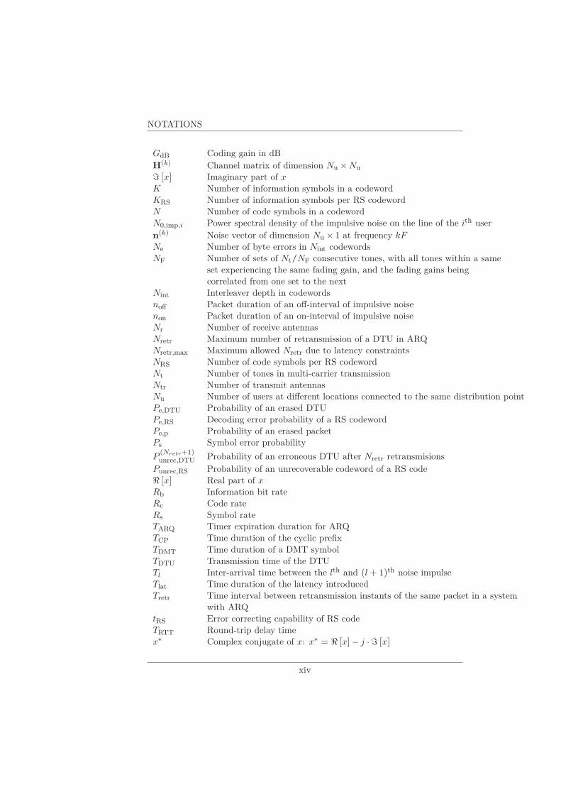
GdB Coding gain in dBH(k) Channel matrix of dimension Nu × Nu
ℑ [x] Imaginary part of x
K Number of information symbols in a codewordKRS Number of information symbols per RS codewordN Number of code symbols in a codewordN0,imp,i Power spectral density of the impulsive noise on the line of the ith usern(k) Noise vector of dimension Nu × 1 at frequency kF
Ne Number of byte errors in Nint codewordsNF Number of sets of Nt/NF consecutive tones, with all tones within a same
set experiencing the same fading gain, and the fading gains beingcorrelated from one set to the next
Nint Interleaver depth in codewordsnoff Packet duration of an off-interval of impulsive noisenon Packet duration of an on-interval of impulsive noiseNr Number of receive antennasNretr Maximum number of retransmission of a DTU in ARQNretr,max Maximum allowed Nretr due to latency constraintsNRS Number of code symbols per RS codewordNt Number of tones in multi-carrier transmissionNtr Number of transmit antennasNu Number of users at different locations connected to the same distribution pointPe,DTU Probability of an erased DTUPe,RS Decoding error probability of a RS codewordPe,p Probability of an erased packetPs Symbol error probability
P(Nretr+1)unrec,DTU Probability of an erroneous DTU after Nretr retransmisions
Punrec,RS Probability of an unrecoverable codeword of a RS codeℜ [x] Real part of x
Rb Information bit rateRc Code rateRs Symbol rateTARQ Timer expiration duration for ARQTCP Time duration of the cyclic prefixTDMT Time duration of a DMT symbolTDTU Transmission time of the DTUTl Inter-arrival time between the lth and (l + 1)th noise impulseTlat Time duration of the latency introducedTretr Time interval between retransmission instants of the same packet in a system
with ARQtRS Error correcting capability of RS codeTRTT Round-trip delay timex∗ Complex conjugate of x: x∗ = ℜ [x] − j · ℑ [x]
xiv

NOTATIONS
x(k) Transmitted vector of dimension Nu × 1 at frequency kF
y(k) Received vector of dimension Nu × 1 at frequency kF
τl Duration of the lth noise impulse
xv


Samenvatting
“Het is onmogelijk niet te communiceren.”
– Paul Watzlawick
De dag van vandaag is digitale communicatie alomtegenwoordig en maaktze een groot deel uit van eenieders leven. Digitale communicatie houdt in datde over te brengen informatie eerst wordt omgezet naar digitale data, zoals bits.Steeds meer toestellen per persoon worden aangesloten op het internet, bijvoor-beeld digitale televisie decoders, smartphones, smart TVs, tablets, sporthor-loges, digitale weegschalen... Kortom het internet is overal. Daardoor is er eenvraag naar steeds meer bandbreedte wat overeenkomt met het verzenden enontvangen van meer data per tijdseenheid. Ook het stijgend aantal toepassin-gen die communiceren over het internet, zoals radio and video streaming, en destijgende video en audio kwaliteit zorgen ervoor dat het dataverkeer toeneemt.
In dit doctoraatsonderzoek hebben we ons hoofdzakelijk gefocust op hettoegangsnetwerk tot het internet. Dit toegangsnetwerk treedt op als bottleneckvoor de bereikbare toegangssnelheid. Al vele jaren spreekt men over de fiber-to-the-home (FTTH) connectie die elke huis rechtstreeks via onzettend snelleglazvezel met het glasvezel kernnetwerk verbindt. Maar in België en vele an-dere landen in Europa (Portugal is de enige uitzondering) bestaat enkel het
xvii

SAMENVATTING
kernnetwerk uit glasvezel. De eindgebruiker is ermee verbonden via een toe-gangsnetwerk van koperen kabels, zoals coaxkabel of telefoonkabel bestaandeuit getwiste paren, soms gevolgd door een draadloos toegangsnetwerk, zoals Wi-Fi of 4G. Ons onderzoek concentreert zich op het verzenden over telefoonkabel,namelijk de DSL lijn, en Wi-Fi. De reden waarom de installering van het FTTHnetwerk uitblijft, is de uitzonderlijk hoge kost die gepaard gaat met het uitrollenvan de glasvezelkabels, meer specifiek voor de nodige wegenwerken, het open-leggen van voetpaden en opritten,... Momenteel wordt de kost gespreid overmeerdere jaren en is er een graduele uitrolling van glasvezel bezig. Daardoorwordt het stuk koper of het toegangsnetwerk dat de eindverbruiker verbindtmet het glasvezel kernnetwerk wel steeds korter. Het kortere toegangsnetwerkbrengt verschillende opportuniteiten met zich mee. Op een kortere koperdraadis de verzwakking van de hogere frequenties lager en doordoor kan er een groterebandbreedte worden gebruikt dan voorheen.
Doorgaans liggen de kabels die buren in eenzelfde straat bedienen naastelkaar in een binder. Doordat de kabels dicht bij elkaar liggen treedt er vaakoverspraak op, dit wil zeggen dat het signaal afkomstig uit de ene kabel in-terfereert met het signaal in de andere kabels. Voor lage frequenties is dezeoverspraak meestal klein, maar voor de hogere frequenties kan het voorkomendat de overspraak, afkomstig van de andere kabels in de binder, sterker is danhet rechtstreeks of oorspronkelijk signaal. Dit kan worden opgelost met eentechniek die precoding heet. We bekijken twee soorten precoding, nl. lineaireen niet-lineaire. Ons doel is om een zo hoog mogelijke bitsnelheid te halen bin-nen bepaalde vooropgelegde limieten in vermogen. Om dit te bereiken hebbenwe twee algoritmes voorgesteld, namelijk het column-norm scaling (CNS) al-goritme en het extended Zanatta-Filho (EZF) algoritme, die de bits verdelenover de beschikbare dragers op zo een wijze dat er met het beschikbaar ver-mogen zoveel mogelijk bits worden verstuurd. Dit is niet voor de hand liggendomdat bits alloceren op een drager voor een bepaalde gebruiker gevolgen heeftop de andere tonen en voor de andere gebruikers (zijn buren) omwille van deoverspraak.
Natuurlijk willen we dat de verzonden bits correct aankomen bij de ont-vanger en dat de ontvangen informatie overeenkomt met wat verstuurd was.Het optreden van bitfouten wordt veroorzaakt door witte ruis en impuls ruisop de koperkabel. Op het draadloos netwerk kan het signaal verzwakt wor-den door het optreden van fading. Dit alles bemoeilijkt het detecteren van debits. Om binnen zulke omstandigheden toch op een betrouwbare manier in-formatie te verzenden, beschouwen we verschillende foutcorrigerende codes enretransmissieprotocols om de verzonden data te beschermen en analyseren hunprestatie.
Op de DSL lijn kunnen we concluderen dat het gebruik van de niet-lineaireprecoder resulteert in hogere bitsnelheden dan de lineaire precoder. Daarnaastprefereren we het CNS bitallocatie algoritme boven het EZF algoritme, ook al
xviii

SAMENVATTING
halen we er iets lagere bitsnelheden mee, de bitverdeling gebeurt aan een veellagere rekencomplexiteit. Bovendien halen we voordeel uit het toevoegen vanerror controle aan ons systeem in vergelijking met ongecodeerde transmissie.Low-density parity-check (LDPC) codes halen het van de andere vooropgesteldebeschermingsstrategieën (trellis-coded modulation (TCM), de opeenvolging vanTCM met byte interleaver en RS code). We bekomen de hoogste bitsnelhedenmet de LDPC codes van hoge coderate, i.e. R = 5/6, 16/18 en 20/21, waarbijhet afhangt van het niveau van impulsruis welke coderate verkozen wordt.
Ook de toepassing van retansmissieprotocols bevordert de connectiesnelheid.Het vernietigende effect van het occasioneel optreden van impulsruis wordt ver-holpen door gebruik van selective-repeat automatic-repeat-request (SR-ARQ);pakketten die verloren zijn worden opnieuw verzonden. In de afwezigheid vanimpulsruis halen we een klein bitsnelheidsvoordeel bij de mogelijkheid tot éénretransmissie. Indien er wel impulsruis optreedt, halen we een serieus voordeelin bitsnelheid indien een maximum van 4 retransmissies is toegestaan.
In het geval van draadloze communicatie wordt de betrouwbaarheid ver-hoogd door een hogere diversiteit. Dit wil zeggen dat verschillende versies vanhet zelfde bericht de ontvanger bereiken via verschillende paden. Diversiteitkan verkregen worden door gebruik te maken van multiple-input multiple-output(MIMO) systemen, wat overeenkomt met meerdere zend- en ontvangstantennes,in combinatie met orthogonale spatio-temporele blokcodes (OSTBCs) en doorhet gebruik van SR-ARQ. Beide systemen brengen kosten met zich mee, namelijkrespectievelijk een hardware kost bij een toename van het aantal antennes, en dekost van een groter buffergeheugen. Een afweging kan gemaakt worden tussenbeide technieken om de vereiste diversiteit te bereiken.
We beëindigen dit proefschrift met een samenvatting van de belangrijksteresultaten en stellen enkele onderwerpen voor om dit onderzoek verder uit tebreiden, zoals Hybrid ARQ en Raptor codes.
xix


Summary
“One cannot not communicate.”
– Paul Watzlawick
Nowadays digital communication is ubiquitous and largely present in ev-eryone’s lifes. Digital communications implies that prior to transmission, theinformation to be transferred is converted to digital data, like bits. More andmore devices per user are connected to the internet, e.g., digital television de-coders, smart phones, smart TVs, tablets, sport watches, digital scales,. . . Toput it briefly, the internet is everywhere. This causes an increase for ever morebandwidth, corresponding to the transmission and reception of more data pertime unit. Also the growing number of applications that communicate over theinternet, like radio and video streaming, and the increasing quality of audio andvideo make that the data traffic increases.
In this dissertation, we are mainly focused on the access network to the
internet. This access network serves as a bottleneck to the achievable access
speed. Already for many years, fiber-to-the-home (FTTH) is mentioned as the
link that connects every house directly via immense fast fiber to the fiber core
network. But in Belgium and many other countries in Europe (Portugal is the
only exception), only the core network consists of fiber links. The end user is
xxi

SUMMARY
connected to it through an access network consisting of copper cables, like coaxand twisted-pair telephone-cable, sometimes followed by a wireless access net-work like Wi-Fi or 4G. The reason for the delay of the FTTH network installa-tion is the exceptional high costs associated with deployment of the fiber cables,i.e. the required roadworks, breaking up pavements and driveways,. . . Currently,this cost is spread over several years and there is a gradual deployment of fiber.This makes that the copper link that connects the end user with the fiber corenetwork, is getting shorter. The shorter access network has several opportuni-ties. The higher frequencies are less diminished and this lets us use a largerbandwidth than before.
Usually cables that serve neighbours in a single street are co-located in abinder. The presence of nearby cables in the binder causes the occurrence ofcrosstalk. This means that the signal from one cable interferes with the signalin the other cables. Crosstalk is usually small at the lower frequencies. At thehigher frequencies, it is possible that the crosstalk originating from the othercables in the binder, is stronger than the original signal. This crosstalk canbe canceled by applying a technique called precoding. We consider both linearand non-linear precoding. We target a maximization of the bit rate, subjectto power limitations. To achieve this, we propose two bitloading algorithms,i.e. the column-norm scaling (CNS) algorithm and the extended Zanatta-Filho(EZF) algorithm, that allocate the bits on the available tones such that asmany bits as possible are transmitted with the available power. This is not atall obvious, as allocating bits on one tone has consequences for the other tonesand users (his neighbours) due to the crosstalk.
Of course, it is desired that the transmitted bits reach the receiver withouterrors and that the received information matches with what was transmitted.The occurrence of bit errors is caused by white noise and impulsive noise on thecopper cable. On the wireless channel, the signal might be distorted due to theoccurrence of fading. All this complicates the detection of the bits. To be ableto reliably transmit information in these circumstances, we consider differenterror correcting codes and retransmission protocols to protect the transmitteddata and we analyze their performance.
On the DSL line, we conclude that the use of the non-linear precoder resultsin higher bit rates than the linear precoder. Furthermore, we prefer the CNSalgorithm above the EZF algorithm. Although, it achieves a minor lower bitrate, the algorithm runs at a major computation complexity reduction. More-over, we obtain advantage from the addition of error control to our system ascompared to uncoded transmission. Low-density parity-check (LDPC) codesbeat the other proposed protection strategies (trellis-coded modulation (TCM),the concatenation of TCM with byte-interleaver and RS code). We achieve thehighest bit rates with the LDPC codes of higher rate, i.e. R = 5/6, 16/18en 20/21, where it depends on the level of impulsive noise which code rate ispreferred.
xxii

SUMMARY
Also, the application of retransmission protocols improves the connectionspeed. The destroying impact of the occasional occurrence of impulsive noiseis tackled by the use of selective-repeat automatic-repeat-request (SR-ARQ);lost packets are retransmitted. In the absence of impulsive noise, we obtain asmall increase in bit rate by the allowance of one retransmission. If impulsivenoise is present, a huge advantage is possible in bit rate if a maximum of 4retransmissions is allowed.
In the case of wireless communication, the reliability is increased by a higherdiversity. This implies that different replicas of the same message reach thedestination through different paths. Diversity can be obtained by the use ofmultiple-input multiple-output (MIMO), which corresponds to several send andreceive antennas, in combination with orthogonal space-time block codes (OS-TBCs) and through the use of SR-ARQ. Both systems come with a cost, i.e.respectively a hardware cost associated with an increase of antennas and the costof a larger retransmission buffer. A trade-off exists between both techniques, inorder to achieve the required diversity order.
We finish this dissertation with a concluding summary of the most importantresults and propose some subjects for future research, such as Hybrid ARQ andRaptor codes.
1

SUMMARY
2

1Introduction
In this dissertation, we study the effect of error protection strategies and pre-coding techniques on the error performance and quality of service of the endapplication. We present some bitloading algorithms to maximize the error freethroughput. This doctoral thesis consists of two separate although related parts.
In the first part, we consider transmission over DSL channels and examinewhich precoding and protection strategy is preferred to obtain the highest pos-sible throughput. In the second part, the topic is shifted to the transmission ofvideo over an indoor wireless channel subject to Rayleigh fading.
In Section 1.1, we give some background on the notion ’digital communica-tion system’. Section 1.2 gives the motivation for this work and the outline ofthis thesis is presented in Section 1.3.
1.1 Background
In a digital communication system, a transmitter wants to transmit informationbits over a transmission medium to a receiver as visualized in the block diagramin Figure 1.1. The information bits may originate from an analog or digital
3

1. INTRODUCTION
Transmitter Transmission
Medium Receiver
information bits
retrieved
information bits
Figure 1.1: Block diagram of a general digital communication system.
source, and from any kind of application such as a website, a music station, avideo game, telephone or e-mail. In the case of a telephone call, the voice comestypically from an analog source (a human) and is converted to informationbits by an analog to digital converter (ADC). Also the transmission mediumor channel can be of all kinds; e.g., the twisted-pair telephone line, coax cable,fiber, satellite connection, Wi-Fi network,... Our work is focused on two of thesechannels; i.e. the twisted-pair telephone line in Part I and the Wi-Fi networkin Part II of this dissertation.
The transmitter transforms the information bits into a physical signal (e.g.,optical signal, electromagnetic signal,...) that needs to be transmitted over thechannel. The receiver observes the physical signal at the output of the channel,tries to reconstruct the information bits and outputs them to the application.On the channel, several sources of distortion may disturb the transmitted sig-nal, like interference from other signals and noise. Therefore, the signal at thereceiver side is likely to differ from the original transmitted signal. In this way,it is possible that the recovered information bits at the receiver are not equalto the original information bits at the transmitter.
In a good communication system, the system is designed so that with highprobability the recovered information bits equal the original transmitted bits.Various techniques can be applied. For example, redundancy can be added tothe transmitted information bits, so that, in spite of some erroneous bits at thereceiver, the information bits can still be recovered (forward error correction(FEC)). Also retransmissions may be scheduled if the received bits are detectedto be erroneous (automatic repeat request (ARQ)); the transmitter sends afternotification a new copy of the original transmitted information bits.
Of course, transmitting information requires energy. An increase of powerimproves the received signal quality. But increasing the transmission energy isnot always desirable, as it causes the transmitted signal to interfere more withother signals, and using less power is considered beneficial in a "green" world.Also, the transmit power of wireless communications is subject to regulationsdesigned to limit the exposure to protect the public health. We want to use thetransmission medium as efficient as possible; i.e., to achieve the required QoSwith the least possible transmit energy.
4
1.2. MOTIVATION
1.2 Motivation
Prediction states that IP traffic will grow with 23 % from 2014 to 2019 [1].
Clearly, the bit rate demand is still increasing fast. The average number of
devices per user grows, and expected is a growth in especially IP traffic from
other devices than PCs; i.e. smartphones, TVs, tablets,...
Already many years ago, fiber-to-the-home (FTTH) was mentioned as the
next very high-speed (speed of several Gbps) internet connection as fiber can
carry data at very high speed over large distances. But due to the excessive
costs that are needed to install fiber into all homes (breaking open pavements
and driveways, road works,...), the fiber installation is spread over a longer
time period and the deployment is gradually. The current broadband network
infrastructure consists mainly of a fiber aggregation network with a copper ac-
cess network that connects the end user with the fiber termination. The access
network is the bottleneck to the achievable bit rate that the end user experi-
ences. Thanks to the gradual deployment of fiber in the network, the access
network becomes shorter and shorter and new challenges and opportunities to
employ the channel become available. The shorter copper loop allows to use a
higher bandwidth, so that new techniques can be applied to efficiently exploit
the increased bandwidth.
In the second part of this thesis, we deal with a different challenge but use
similar techniques as in the first part. Transmission over a wireless channel is
subject to fading which may cause bursts of erroneous bits if a deep fade arises.
The transmission of video, more specifically high definition television (HDTV)
must meet severe restrictions on latency and only a limited number of visual
distortions per time interval is allowed, in order to satisfy the required quality
of service (QoS).
1.3 Outline
This dissertation is organized as follows.
Chapter 2 presents some general and basic concepts of forward error correction
schemes and automatic repeat request protocols.
Part I
Chapter 3 gives an introduction on the transmission over the DSL channel. It
gives an overview of the history of DSL and discusses two sources of noise from
which transmission over DSL suffers.
Chapter 4 describes the system model as it is used throughout Part I of this
thesis. A mathematical description of the system with crosstalk is provided,
and the different precoding techniques to deal with this crosstalk are presented.
Furthermore, the reader will find in this chapter an overview of the constellation
5

1. INTRODUCTION
types used and a statistical model for the impulsive noise.Chapter 5 investigates the error performance with linear and nonlinear pre-coding for uncoded transmission and various types of coded transmission.Chapter 6 presents two bitloading algorithms for linear and nonlinear precod-ing under simultaneous aggregate transmit power and power spectral densityconstraints.Chapter 7 provides the resulting error free throughputs for the system withoutimpulsive noise and application of the different precoders, bitloading algorithmsand coding schemes and concludes how the system should be designed in theabsence of impulsive noise.Chapter 8 extends the results from Chapter 7 by including impulsive noise,and concludes which error protection scheme is preferred in presence of impul-sive noise.
Part II
Chapter 9 analyzes application layer ARQ for the protection of video packetsover an indoor MIMO-OFDM link with correlated block fading. We examinea suitable form of error control to protect video packets against losses and tomaintain a sufficient quality of experience for the end user watching the video.
Chapter 10 summarizes the conclusions of the obtained results. Furthermore,
it proposes some topics for future research, that fell outside the scope of this
dissertation. This chapter wraps up with a complete list of our publications.
6

2Error Control
In this chapter, we introduce some general concepts of forward error correction(FEC) schemes and automatic request (ARQ) protocols. In Section 2.1, we startwith uncoded transmission, the performance of which we will use as a bench-mark for coded transmission. Sections 2.2 and 2.3 provide some backgroundinformation about respectively trellis-coded modulation (TCM) and low-densityparity-check (LDPC) codes. Reed-Solomon (RS) coding is introduced in Section2.5. Sections 2.6 and 2.7 discuss respectively interleaving and ARQ. Section 2.8presents the performance indicators which will be used in this dissertation.
2.1 Uncoded Transmission
In uncoded transmission, there is no channel encoder present and no redundancyis added to the information bit stream to be transmitted. The information bitstream is mapped to constellation symbols, modulated on waveforms and trans-mitted over the channel. On the channel, the signals are subject to noise andinterference. Besides the Euclidean distance between the constellation points,that for a given constellation depends on the symbol energy, there is no protec-tion that might increase the reliability of the transmitted data. At the receiver,
7

2. ERROR CONTROL
the received signals are demodulated, yielding noisy complex symbols. Harddecision on the noisy symbols is performed: the receiver assumes that the con-stellation point closest (in terms of Euclidean distance) to the received noisysymbol value was transmitted.
The addition of reduncancy by a channel encoder serves to increase thereliability of the received data but, unlike uncoded transmission, decreases theinformation bitrate for a given signal constellation.
2.2 Basic Principles of TCM
Trellis-coded modulation (TCM) is a commonly applied technique for combinedcoding and modulation in bandwidth-constrained channels. A coding gain canbe achieved without increasing the signal bandwidth, compared to uncodedtransmission. The redundancy introduced by the code is achieved by expand-ing the constellations. The modulation and coding are jointly optimized tomaximize the Euclidean distance between coded symbol sequences by using setpartitioning as described in Section 2.2.1.
TCM was first proposed in 1976 by Ungerboeck [2], but became well adoptedand researched in 1982 only, when a more detailed publication of Ungerboeck [3]appeared.
Figure 2.1: Gottfried Ungerboeck (born March 15, 1940, Vienna, Austria).
Since then, TCM has been employed in many digital transmission systemswith higher-order constellations, i.e., modulation schemes that transmit morethan one bit per channel use, such as PSK and QAM. As far as digital subscriberline (DSL) systems are concerned, TCM has been adopted first in the single-pair high-speed DSL (SHDSL) standard [4], and remains an essential ingredientin the transceivers up to the most recently deployed very high speed DSL 2(VDSL2) standard [5]. For more information about the DSL standards, thereader is referred to Section 3.1.
8

2.2. BASIC PRINCIPLES OF TCM
2.2.1 Set Partitioning
To maximize the minimum Euclidean distance between the coded symbol se-quences in TCM, an appropriate mapping of the coded bits to constellationsymbols has to be determined. Such a mapping method was developed byUngerboeck [3], called set partitioning.
Consider a trellis encoder, which encodes m incoming information bits tom + 1 encoded bits. These coded bits are mapped on constellation symbolsfrom a symbol constellation A, containing 2m+1 symbol points. This symbolconstellation is partitioned into subsets in a way that the minimum Euclideandistance between the points in a subset is increased with each partitioning step.The subsets resulting from a given partitioning step have equal size. This tech-nique is illustrated in Figure 2.2 for 16-QAM.
1
1 1
1 1 1 1
1 1 1 1 1 1 1
1
0
0 0
0 0 0 0
0 0 0 0 0 0 0 0
0000 1000 0100 1100 0010 1010 0110 1110 0001 1001 0101 1101 0011 1011 0111 1111
Figure 2.2: Set partitioning of 16-QAM.
In a first step, the 16-QAM constellation is partitioned into two subsetsof 8 points each, by assigning two neighbouring points at minimum distanceto different subsets. This way, the minimum squared Euclidean distance isincreased from d2 (for the original constellation) to 2d2. Each partitioning stepin a squared constellation doubles the minimum squared Euclidean distancein the resulting subsets. Further partitioning of each subset divides again thepoints alternating in two separate subsets and the minimum squared Euclideandistance is increased to 4d2. After the fourth and last partitioning, each of the16 subsets contains one remaining constellation point. The minimum squaredEuclidean distance in these subsets is defined to be +∞. In this example, thepartitioning consists of four steps, until no further partitioning is possible andeach subset contains one symbol point. In general the partitioning can stopafter less than he maximum possible number of steps, as explained in Section2.2.2.
9

2. ERROR CONTROL
Select symbol
in subset
Select subset
Rate K/(K+1)
convolutional
encoder
)(
1
lu
)(
2
lu
)(l
Ku
)(
1
lc
)(
2
lc
)(
1
l
+Kc
)(lcS
)(
1
l
+Ku
)(
2
l
+Ku
)(l
mu
Constellation
symbol
Figure 2.3: General structure of TCM encoder.
2.2.2 General Structure of TCM Encoder
Figure 2.3 shows the general structure of the TCM encoder, which transformsm information bits into a symbol from a constellation A that contains 2m+1
points. From the m information bits u(ℓ) = (u(ℓ)m ,u
(ℓ)m−1, . . . ,u
(ℓ)1 ) that enter
the encoder at time ℓ, the K least significant bits (u(ℓ)K ,u
(ℓ)K−1, . . . ,u
(ℓ)1 ) are
encoded using a rate K/(K + 1) binary convolutional encoder, with K ≤ m.
The encoder produces K + 1 coded bits c(ℓ) = (c(ℓ)K+1, c
(ℓ)K , . . . , c
(ℓ)1 ). A number
of K + 1 partitioning steps are applied to the constellation A, yielding 2K+1
subsets, each containing 2m−K constellation points. When K < m, the m − K
most significant bits u′(ℓ) = (u(ℓ)m ,u
(ℓ)m−1, . . . ,u
(ℓ)K+1) remain uncoded and are
sent together with the coded bit vector c(ℓ) to the symbol mapper. The symbolmapper converts (u′(ℓ), c(ℓ)) into a constellation symbol that belongs to A. Thesubset S
c(ℓ)of the constellation A is selected by the coded bit vector c(ℓ), while
u′(ℓ) picks the resulting constellation point among the 2m−K symbols in thesubset S
c(ℓ).
2.2.3 Convolutional Encoding
Convolutional codes were first proposed by Elias in 1955 [6]. A convolutionalencoder of rate Rc = K/N is shown in Figure 2.4. The encoder contains K
shift registers, each containing L − 1 delay blocks; L is called the constraintlength of the code. The N coded bits are obtained as modulo-2 sums of bitsfrom the K shift registers; these sums are defined by the N generator sequences
g(j)i = (g
(j)i,0 , g
(j)i,1 , . . . , g
(j)i,L−1)
10

2.2. BASIC PRINCIPLES OF TCM
K information bits
D D D
D D D
D D D
P/S N code bits
�
S/P �
L-1 delay blocks per shift register
Figure 2.4: General rate K/N convolutional encoder.
Figure 2.5: Peter Elias (November 23, 1923, New Jersey – December, 7 2001).
with i = 1, . . . ,K, j = 1, . . . ,N and g(j)i,l ∈ {0, 1}. These generator sequences
determine which of the delay-block outputs are connected to which modulo-2
adders, as visualized in Figure 2.4. For g(j)i,l = 1, the lth delay block output from
the ith register is connected to the jth modulo-2 adder. For g(j)i,l = 0, there is
no connection. Taking l = 0 refers to the current input without delay.
The register is initialized to all-zero. The information bit sequence is de-multiplexed by a serial-to-parallel convertor (S/R) into K lower-rate sequenceswhich are fed to the K registers. At discrete instant ℓ, the ith register contains
the L information bits (u(ℓ)i , . . . ,u
(ℓ−L+1)i ), and a N bit output vector is pro-
duced by applying a parallel-to-serial convertor (P/S) to the N modulo-2 sums
11
2. ERROR CONTROL
D D )(
1
lu
)(
2
lc
)(
1
lc
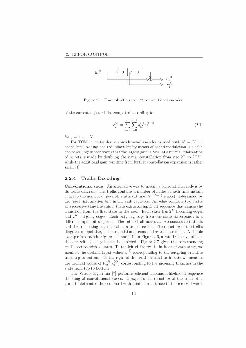
Figure 2.6: Example of a rate 1/2 convolutional encoder.
of the current register bits, computed according to
c(ℓ)j =
K∑
i=1
L−1∑
l=0
g(j)i,l u
(ℓ−l)i (2.1)
for j = 1, . . . ,N .For TCM in particular, a convolutional encoder is used with N = K + 1
coded bits. Adding one redundant bit by means of coded modulation is a solidchoice as Ungerboeck states that the largest gain in SNR at a mutual informationof m bits is made by doubling the signal constellation from size 2m to 2m+1,while the additional gain resulting from further constellation expansion is rathersmall [3].
2.2.4 Trellis Decoding
Convolutional code An alternative way to specify a convolutional code is byits trellis diagram. The trellis contains a number of nodes at each time instantequal to the number of possible states (at most 2K(L−1) states), determined bythe ’past’ information bits in the shift registers. An edge connects two statesat successive time instants if there exists an input bit sequence that causes thetransition from the first state to the next. Each state has 2K incoming edgesand 2K outgoing edges. Each outgoing edge from one state corresponds to adifferent input bit sequence. The total of all nodes at two successive instantsand the connecting edges is called a trellis section. The structure of the trellisdiagram is repetitive, it is a repetition of consecutive trellis sections. A simpleexample is shown in Figures 2.6 and 2.7. In Figure 2.6, a rate 1/2 convolutionaldecoder with 2 delay blocks is depicted. Figure 2.7 gives the correspondingtrellis section with 4 states. To the left of the trellis, in front of each state, we
mention the decimal input values u(ℓ)1 corresponding to the outgoing branches
from top to bottom. To the right of the trellis, behind each state we mention
the decimal values of (c(ℓ)2 , c
(ℓ)1 ) corresponding to the incoming branches in the
state from top to bottom.The Viterbi algorithm [7] performs efficient maximum-likelihood sequence
decoding of convolutional codes. It exploits the structure of the trellis dia-
gram to determine the codeword with minimum distance to the received word.
12

2.2. BASIC PRINCIPLES OF TCM
0
1
2
3
0
1
2
3
0 1
0 1
0 1
0 1
0 2
1 3
2 0
3 1
Figure 2.7: Trellis section corresponding to the convolutional encoder in theexample from Figure 2.6.
Figure 2.8: Andrew Viterbi (born March 9, 1935, Bergamo, Italy).
A search of possible paths through the trellis has to be completed. On eachedge, the metric for this search is the corresponding squared Euclidean distancebetween the noisy received symbols and the output symbols for the current tran-sition. If two or more paths enter the same state, only the path with minimumcumulated squared Euclidean distance is kept.
TCM In TCM, the presence of uncoded bits gives rise to parallel transitionsin the trellis diagram. The trellis diagram of TCM is given by the trellis fromits convolutional code where each state transitions turns into 2m−K paralleltransitions, as the state transition is solely determined by the current state and
the current input bits of the convolutional encoder. If two input vectors u(ℓ)1
and u(ℓ)2
differ only in the uncoded bits (u(ℓ)m ,u
(ℓ)m−1, . . . ,u
(ℓ)K+1), they will result
in the same state transition. Thus, all symbol points from one subset Sc(ℓ)
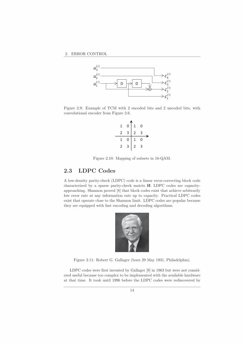
correspond to parallel transitions in the trellis diagram. Figure 2.9 shows anexample for TCM with the convolutional encoder from Figure 2.6 with 4 bits atthe output. The corresponding set partitioning of 16-QAM is depicted in Figure2.10. The constellation points are labeled by the decimal value of the two bits
(c(ℓ)2 , c
(ℓ)1 ) according to the subset they belong to.
The Viterbi algorithm is analogues for TCM as for a convolutional code. Thepresence of parallel transitions is solved by only retaining the transition withminimum Euclidean distance from all parallel transitions between two states.
13
2. ERROR CONTROL
D D )(
1
lu
)(
2
lc
)(
1
lc
)(
2
lu
)(
3
lu
)(
4
lc
)(
3
lc
Figure 2.9: Example of TCM with 2 encoded bits and 2 uncoded bits, withconvolutional encoder from Figure 2.6.
1 0
2 3
1
2
0
3
1 0
2 3
1 0
2 3
Figure 2.10: Mapping of subsets in 16-QAM.
2.3 LDPC Codes
A low-density parity-check (LDPC) code is a linear error-correcting block codecharacterized by a sparse parity-check matrix H. LDPC codes are capacity-approaching. Shannon proved [8] that block codes exist that achieve arbitrarilylow error rate at any information rate up to capacity. Practical LDPC codesexist that operate close to the Shannon limit. LDPC codes are popular becausethey are equipped with fast encoding and decoding algorithms.
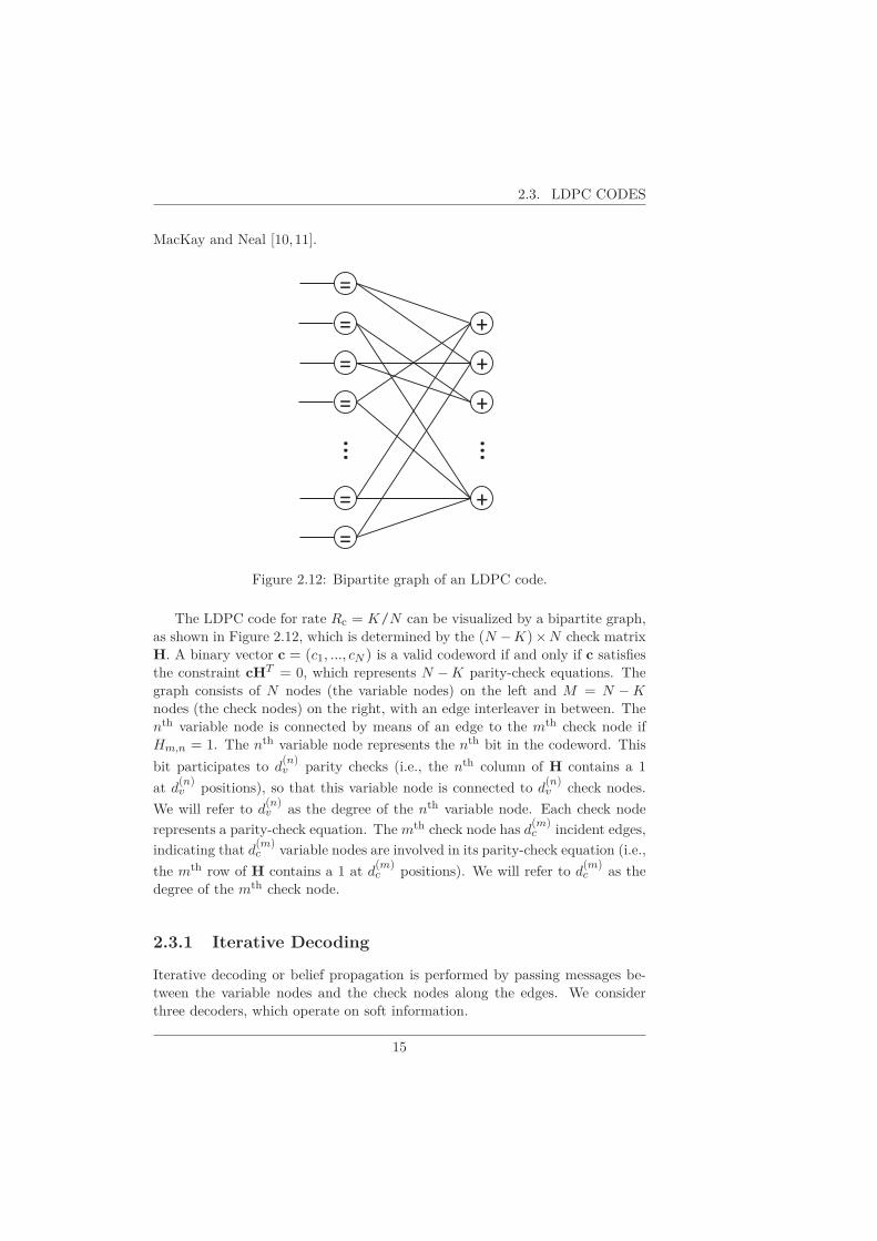
Figure 2.11: Robert G. Gallager (born 29 May 1931, Philadelphia).
LDPC codes were first invented by Gallager [9] in 1963 but were not consid-ered useful because too complex to be implemented with the available hardwareat that time. It took until 1996 before the LDPC codes were rediscovered by
14
2.3. LDPC CODES
MacKay and Neal [10,11].
=
=
=
=
=
=
�
+
+
+
�
+
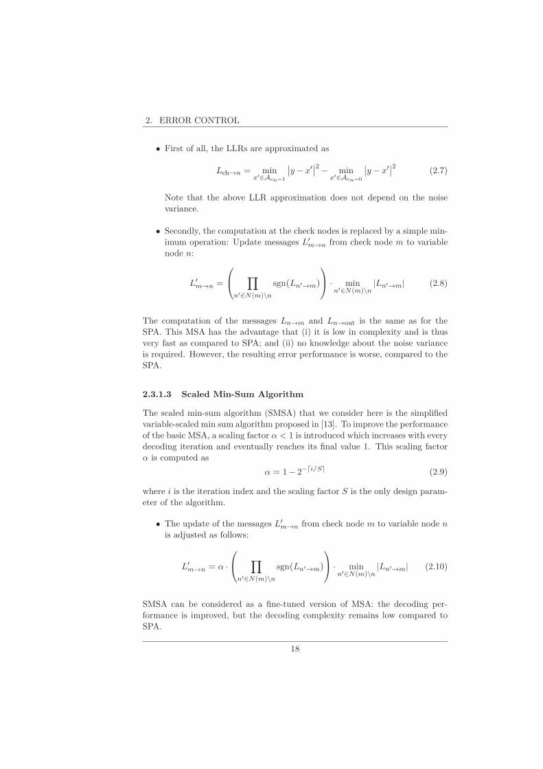
Figure 2.12: Bipartite graph of an LDPC code.
The LDPC code for rate Rc = K/N can be visualized by a bipartite graph,as shown in Figure 2.12, which is determined by the (N − K)× N check matrixH. A binary vector c = (c1, ..., cN ) is a valid codeword if and only if c satisfiesthe constraint cHT = 0, which represents N − K parity-check equations. Thegraph consists of N nodes (the variable nodes) on the left and M = N − K
nodes (the check nodes) on the right, with an edge interleaver in between. Thenth variable node is connected by means of an edge to the mth check node ifHm,n = 1. The nth variable node represents the nth bit in the codeword. This
bit participates to d(n)v parity checks (i.e., the nth column of H contains a 1
at d(n)v positions), so that this variable node is connected to d
(n)v check nodes.
We will refer to d(n)v as the degree of the nth variable node. Each check node
represents a parity-check equation. The mth check node has d(m)c incident edges,
indicating that d(m)c variable nodes are involved in its parity-check equation (i.e.,
the mth row of H contains a 1 at d(m)c positions). We will refer to d
(m)c as the
degree of the mth check node.
2.3.1 Iterative Decoding
Iterative decoding or belief propagation is performed by passing messages be-tween the variable nodes and the check nodes along the edges. We considerthree decoders, which operate on soft information.
15

2. ERROR CONTROL
2.3.1.1 Sum-Product Algorithm
The sum-product algorithm (SPA) was developed by MacKay and Neal [11]and gives excellent decoding results. The algorithm operates on log-likelihoodratios (LLRs), which represent soft information of the coded bits, derived fromobserving the channel output. At initialization, all messages on the edges of the
Figure 2.13: David MacKay (April 22, 1967, Stoke-on-Trent, U.K. – April 14,2016).
Tanner graph are set to 0. Next, the LLRs of the N coded bits are computedfrom the channel observations; this operation is referred to as soft demapping.Let us consider an AWGN channel characterized by y = x + w, where x is asymbol drawn from a constellation A representing b bits (among which the codedbit cn), and w is complex-valued additive white Gaussian noise with variance2σ2. The LLR Lch→n related to the nth coded bit cn is defined as
Lch→n = lnp(y|cn = 0)
p(y|cn = 1)n = 1, . . . ,N (2.2)
where p(y|cn) is the conditional probability density of the channel output y
given the value of the coded bit cn. For the considered channel model, (2.2)reduces to
Lch→n = ln
∑
x′∈Acn=0
exp(
− 12σ2
|y − x′|2)
∑
x′∈Acn=1
exp(
− 12σ2
|y − x′|2) (2.3)
where Acn=0 and Acn=1 represent the subsets of the symbol constellation A,corresponding to cn = 0 and cn = 1, respectively.
We denote by N (m) = {n : Hm,n = 1} the set of variable nodes that areconnected by an edge to check node m, and by M (n) = {m : Hm,n = 1} theset of check nodes that are connected by an edge to variable node n.
We iterate from variable nodes to check nodes and back until some stoppingcondition is fulfilled. A decoding iteration consists of following two steps:
16

2.3. LDPC CODES
• Update messages Ln→m from variable node n to check node m:
Ln→m = Lch→n +∑
m′∈M(n)\m
L′m′→n (2.4)
• Update messages L′m→n from check node m to variable node n:
L′m→n = 2 tanh−1
∏
n′∈N(m)\n
tanh
(Ln′→m
2
)
(2.5)
The output messages of the decoding process are computed as follows after everyiteration:
• Update messages Ln→out from variable node n to the output:
Ln→out = Lch→n +∑
m∈M(n)
L′m→n (2.6)
which corresponds to the logarithm of the a posteriori probability ratio ofthe nth coded bit cn.
The decoder makes a hard decision for the nth coded bit; this decision is equal to0 if Ln→out > 0 and 1 otherwise. The iterations are stopped when the vector ofN decisions is a valid codeword (i.e., when this vector satisfies the parity-checkequations), or when the maximum number of iterations is achieved.
Note that during the iterations, the values of the LLR messages Lch→n do notchange: the soft demapping is not iterative. In principle, the decoding perfor-mance can be improved by performing iterative soft demapping. In this case, themessages Lch→n are updated with each iteration, based on the messages L′
m→n′
for all m ∈ M (n′) and all n′ for which the corresponding coded bits cn′ belongto the same constellation symbol as the considered bit cn. However, applyingiterative soft demapping considerably increases the computational complexityof the decoding process (especially when using large constellations), whereas itcan be shown that in the case of Gray mapping the performance gain is verysmall. In this dissertation we consider Gray mapping (or a close approximationthereof), and restrict our attention to non-iterative soft demapping in order tolimit the computational complexity.
Two major drawbacks of the SPA are: (i) the noise variance must be known;and (ii) its computational complexity is high (even with non-iterative soft demap-ping), especially for large constellations, because of the tanh(.) and tanh−1(.)operations and the computation (2.3) of the LLRs.
2.3.1.2 Min-Sum Algorithm
The min-sum algorithm (MSA) [12] is similar to the SPA, with a few adjustmentsto reduce the complexity and to make the computations independent of the noisevariance.
17
2. ERROR CONTROL
• First of all, the LLRs are approximated as
Lch→n = minx′∈Acn=1
∣∣y − x′∣∣2 − min
x′∈Acn=0
∣∣y − x′∣∣2 (2.7)
Note that the above LLR approximation does not depend on the noisevariance.
• Secondly, the computation at the check nodes is replaced by a simple min-imum operation: Update messages L′
m→n from check node m to variablenode n:
L′m→n =
∏
n′∈N(m)\n
sgn(Ln′→m)
· minn′∈N(m)\n
|Ln′→m| (2.8)
The computation of the messages Ln→m and Ln→out is the same as for theSPA. This MSA has the advantage that (i) it is low in complexity and is thusvery fast as compared to SPA; and (ii) no knowledge about the noise varianceis required. However, the resulting error performance is worse, compared to theSPA.
2.3.1.3 Scaled Min-Sum Algorithm
The scaled min-sum algorithm (SMSA) that we consider here is the simplifiedvariable-scaled min sum algorithm proposed in [13]. To improve the performanceof the basic MSA, a scaling factor α < 1 is introduced which increases with everydecoding iteration and eventually reaches its final value 1. This scaling factorα is computed as
α = 1− 2−⌈i/S⌉ (2.9)
where i is the iteration index and the scaling factor S is the only design param-eter of the algorithm.
• The update of the messages L′m→n from check node m to variable node n
is adjusted as follows:
L′m→n = α ·
∏
n′∈N(m)\n
sgn(Ln′→m)
· minn′∈N(m)\n
|Ln′→m| (2.10)
SMSA can be considered as a fine-tuned version of MSA: the decoding per-formance is improved, but the decoding complexity remains low compared toSPA.
18

2.3. LDPC CODES
2.3.2 EXIT charts
Extrinsic information transfer (EXIT) charts [14, 15] are used to analyze theiterative decoding performance and convergence behavior of LDPC codes, and todesign new LDPC codes. This method is not as accurate as density evolution [16]but its accuracy is reasonably good and the complexity is much lower.
An EXIT chart consists of two EXIT functions, which are related to how themessages during the decoding iterations are processed by the variable nodes andthe check nodes, respectively. The variable node EXIT function and the checknode EXIT function give IE,V as a function of IA,V , and IE,C as a function ofIA,C , respectively, where
• Variable node EXIT function: IE,V is the average (over the N codedbits) of the mutual information I(cn;Ln→m), between the coded bit cn
(corresponding to the considered variable node n) and the "extrinsic"message Ln→m leaving the variable node, when the mutual informationsI(cn;L
′m′→n) for all m′ ∈ M (n)\m, between the coded bit cn and the "a
priori" message L′m′→n entering the variable node, are equal to IA,V ;
• Check node EXIT function: IE,C is the average (over the N codedbits) of the mutual information I(cn;L
′m→n), between the coded bit cn
(correponding to a variable node n connected to the considered checknode m) and the "extrinsic" message L′
m→n leaving the check node, whenthe mutual informations I(cn′ ;Ln′→m) for all n′ ∈ N (m)\n, between thecoded bit cn′ and the "a priori" message Ln′→m entering the check node,are equal to IA,C .
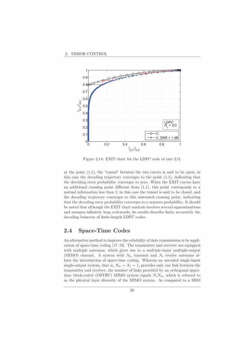
The reader is referred to [14] and [15] for the detailed information on howthe EXIT curves are obtained. The EXIT functions depend on the degreedistributions of the variable nodes and the check nodes of the considered LDPCcode. An example of an EXIT chart is shown in Figure 2.14 for an LDPCcode of rate 2/3, that we will use in Chapter 5. The EXIT chart shows IE,V
(ordinate) as a function of IA,V (abscissa) and IE,C (abscissa!) as a function ofIA,C (ordinate!). The check node EXIT function typically starts in the origin(0,0) and ends in the point (1,1). The variable node EXIT function has a
starting point(
0, IE,V
∣∣IA,V =0
)
and ends in the point (1,1). It can be shown
from (2.4) that the mutual information IE,V
∣∣IA,V =0
equals the average Iavg
(over the N coded bits) of the mutual information I(cn;Lch→n) between thecoded bit cn and the corresponding LLR Lch→n; Iavg depends on the SNRand the considered constellation. Considering that the extrinsic message at theoutput of a variable node (check node) is the a priori message at the input of acheck node (variable node), the exchange of extrinsic information between thevariable nodes and the check nodes can be visualized as a decoding trajectoryin the EXIT chart. The decoding trajectory starts at (0,Iavg), and ends at thecrossing point of the two EXIT curves. When the two EXIT curves cross only
19
2. ERROR CONTROL
0 0.2 0.4 0.6 0.8 10
0.1
0.2
0.3
0.4
0.5
0.6
0.7
0.8
0.9
1
IA,V
,IE,C
I E,V
,IA
,C
C
V, SNR = 1 dB
LDPCR
c = 2/3
Figure 2.14: EXIT chart for the LDPC code of rate 2/3.
at the point (1,1), the "tunnel" between the two curves is said to be open; inthis case the decoding trajectory converges to the point (1,1), indicating thatthe decoding error probability converges to zero. When the EXIT curves havean additional crossing point different from (1,1), this point corresponds to amutual information less than 1; in this case the tunnel is said to be closed, andthe decoding trajectory converges to this unwanted crossing point, indicatingthat the decoding error probability converges to a nonzero probability. It shouldbe noted that although the EXIT chart analysis involves several approximationsand assumes infinitely long codewords, its results describe fairly accurately thedecoding behavior of finite-length LDPC codes.
2.4 Space-Time Codes
An alternative method to improve the reliability of data transmission is by appli-cation of space-time coding [17–19]. The transmitter and receiver are equippedwith multiple antennas, which gives rise to a multiple-input multiple-output(MIMO) channel. A system with Ntr transmit and Nr receive antennas al-lows the introduction of space-time coding. Whereas an uncoded single-inputsingle-output system, that is, Ntr = Nr = 1, provides only one link between thetransmitter and receiver, the number of links provided by an orthogonal space-time block-coded (OSTBC) MIMO system equals NrNtr, which is referred toas the physical layer diversity of the MIMO system. As compared to a SISO
20

2.5. REED-SOLOMON CODES
system, the larger number of links resulting from OSTBC MIMO gives rise toa considerably higher robustness against fading (because of the smaller proba-bility that all links are simultaneously in a deep fade), and a much better errorperformance [18,20].
Unlike most channel codes without spatial redundancy, the OSTBC MIMOsystem does not require additional bandwidth as compared to the uncoded SISOsystem, but comes at a substantial hardware cost that increases with the numberof antennas. Optimum decoding of OSTBC MIMO reduces to linear processingand simple symbol-by-symbol detection at the receiver. In this dissertation,we will consider the Alamouti space-time code [17], which requires 2 transmitantennas (and an arbitrary number Nr of receive antennas). Alamouti space-time coding involves the transmission of two symbols during two consecutiveintervals on two antennas, according to the scheme of Table 2.1, where s1 ands2 represent two symbols, and (.)∗ denotes complex conjugate. Hence, thesymbol si reaches the receiver via 2Nr links (i.e. Nr links for si and Nr links for±s∗
i ).
Table 2.1: Transmitter configuration for Alamouti space-time code.antenna 1 antenna 2
interval 1 s1 s2interval 2 −s∗
2 s∗1
2.5 Reed-Solomon Codes
Reed-Solomon (RS) codes are linear error-correcting block codes presented firstin a paper in 1960 by Irving Reed and Gus Salomon [21]. RS codes are frequentlyused in several fields of application: data storage (compact discs, blu-ray discs),QR codes, deep space communication (Voyager, Galileo), DSL,...
The RS code is defined over the Galois Field GF(2q), which implies that aRS information symbol and code symbol represents q bits; typically, q = 8, inwhich case a symbol corresponds to a byte. The RS codewords have N = 2q − 1
coded symbols.Here we restrict our attention to systematic RS codes, so that the informa-
tion part of the codeword can always be interpreted by the receiver, even inabsence of a RS decoder. Per group of K information symbols, the RS(N ,K)code computes N − K parity symbols resulting in a systematic codeword of N
coded symbols.The RS(N ,K) code is maximum distance separable (MDS), i.e., the mini-
mum Hamming distance between codewords equals N − K + 1, which cannotbe outperformed by any other code with the same number N − K of parity
21

2. ERROR CONTROL
Figure 2.15: Irving Reed (12 November 1923, Washington – 11 September 2012)and Gus Salomon (27 October 1930, Brooklyn — 31 January 1996).
symbols [22, 23]. Hence, the code can correct a combination of e1 symbol er-rors and e2 symbol erasures, provided that 2e1 + e2 ≤ N − K. In the absenceof erasures, up to t =
⌊N−K2
⌋errors can be corrected, and in the absence of
errors, ν = N − K erasures can be resolved. Algebraic algorithms for decodingRS codes can be found in [23–27]. These decoding algorithms look for a valid
RS codeword which differs from the received codeword in at most⌊
N−K−e22
⌋
non-erased positions, with e2 denoting the number of erased symbols; when nosuch codeword is found (because of a too large number of errors/erasures), adecoding failure is declared.
In practice, shortened systematic RS codes are often used. A shortened sys-tematic RS(n, k) codeword is equivalent to a systematic RS(N ,K) codewordwith K − k information symbols set to zero; these K − k zero information sym-bols are not transmitted, yielding a RS(n, k) codeword with the same numberof parity symbols as the original code, so that n = k + (N − K). The minimumHamming distance between codewords of the shortened RS code is the same asfor the original RS code, and equals N − K + 1 = n − k + 1, which indicates
that also the shortened RS codes are MDS; hence, t =⌊
n−k2
⌋
errors can be
corrected in the absence of erasures, and ν = n − k erasures can be resolvedin the absence of errors. The decoding algorithm for the RS(N ,K) code canalso be used for decoding the RS(n, k) code, by simply adding K − k zero infor-mation symbols to the received RS(n, k) codeword, and performing decoding ofthe resulting RS(N ,K) codeword.
In the absence of erasures, a decoding error occurs when the number of sym-
bol errors exceeds t =⌊
n−k2
⌋
. Assuming that symbol errors occur independently
22

2.6. INTERLEAVING
with probability Ps, the decoding error probability Pe,RS is given by [22,23]
Pe,RS =n∑
j=t+1
n!
(n − j)! j!P js (1− Ps)
n−j (2.11)
For small Ps, we have Pe,RS ∝ P t+1s . When the RS decoder declares a decoding
failure, in some applications the k information bytes from the received codewordare forwarded unaltered to the destination; in this case the resulting byte errorrate (ByteER) is obtained as [22,23]
ByteERRS =n∑
j=t+1
(n − 1)!
(n − j)! (j − 1)!P js (1− Ps)
n−j (2.12)
because the probability that a specific byte is erroneous equals j/n when thecodeword has j byte errors.
When only erasures occur, the RS codeword cannot be recovered when thenumber of erasures exceeds ν = n − k. Assuming that symbol erasures occur in-dependently with probability Ps,e, the probability Punrec,RS of an unrecoverablecodeword is given by
Punrec,RS =n∑
j=ν+1
n!
(n − j)! j!P js,e (1− Ps,e)
n−j (2.13)
For small Ps,e, we have Punrec,RS ∝ P ν+1s,e .
2.6 Interleaving
Interleaving (combined with error correction) is a means to cope with bursterrors that exceed the error correcting capability of the code. The informationbit stream is split up into information words, which are sent to a FEC encoder.Typically, a high number (say, Nint) of resulting codewords is then broken upinto smaller parts (bits/bytes/symbols) that are shuffled by an interleaving pro-
cess such that the parts originating from any one of the original codewords
are widely separated in time. At the receiver, the received parts are reshuffled
(’de-interleaved’) so that their original order is restored. The quantity Nint is
referred to as the interleaving depth.
Interleaving aims at spreading each burst of errors over a large number of
codewords such that the resulting number of errors in each codeword is small,
and can hopefully be corrected by the code. Burst of errors can be caused
by impulsive noise as discussed in Section 3.3 or by the inner decoder in a
concatenated coding arrangement, as can happen with trellis decoding using a
Viterbi decoder. Figure 2.16 illustrates the principle.
23

2. ERROR CONTROL
1) no interleaving
A1 A2 A3 A4 B1 B2 B3 B4 C1 C2 C3 C4 Transmitter:
A1 A2 A3 A4 B1 B2 B3 B4 C1 C2 C3 C4 Receiver:
burst of errors
2) with interleaving
A1 B1 C1 A2 B2 C2 A3 B3 C3 A4 B4 C4 Transmitter:
A1 B1 C1 A2 B2 C2 A3 B3 C3 A4 B4 C4 Receiver:
burst of errors
A1 A2 A3 A4 B1 B2 B3 B4 C1 C2 C3 C4
deinterleaver
A1 A2 A3 A4 B1 B2 B3 B4 C1 C2 C3 C4
interleaver
Figure 2.16: Illustration of an interleaver in the occurrence of a burst of errors.
24

2.7. AUTOMATIC REPEAT REQUEST PROTOCOLS
1
1 2 3 2 4 2
1 2 3 2 4 2 Transmitter
Receiver
Figure 2.17: Transmitting with SR-ARQ.
The larger the interleaving depth, the more effective the interleaver. How-ever, the interleaver introduces a latency of Nint codewords, so that the in-terleaving depth is limited by the maximum allowed latency of the particularapplication.
2.7 Automatic Repeat Request Protocols
The automatic repeat request (ARQ) protocol is an adaptive error-control pro-tocol with retransmissions. In this dissertation, we will restrict our attentionto selective-repeat ARQ (SR-ARQ). SR-ARQ enables the receiver to requestthe retransmission of a packet or data transfer unit (DTU) that has been erro-neously received. Each DTU contains (apart from the data) a header includinga sequence number and a cyclic redundancy check (CRC). The CRC enablesthe receiver to detect errors in the received DTU. If a transmitter sends a DTUto a receiver, the following scenarios may occur as illustrated in Figure 2.17:
• The DTU is delivered without errors to the receiver. A positive acknowl-edgment (ACK) is sent to the transmitter.
• The DTU is delivered at the receiver but the CRC fails (shaded DTUs inFigure 2.17). The receiver removes the erroneous DTU and sends a nega-tive acknowledgment (NAK) to the transmitter with the sequence numberof the erased DTU. Typically a maximum number of retransmissions perDTU is allowed, given by Nretr. Upon reception of this retransmission re-quest, and if the maximum number of retransmissions is not yet reached,the transmitter issues the retransmission of a copy of the DTU.
The addition of ARQ as protection strategy leads to an increase of latency. Thelargest latency occurs when the maximum number of retransmissions Nretr isrequired (i.e., the first transmission and the subsequent Nretr −1 retransmissionsof the DTU are erroneous) and is given by
Tlat = TDTU + Nretr (TDTU + TRTT) (2.14)
25

2. ERROR CONTROL
where TDTU is the transmission time of the DTU and TRTT is equal to theround-trip delay time given by
TRTT = 2Tprop + Tproc + Tack (2.15)
with Tprop, Tproc and Tack respectively equal to the propagation time, the totalprocessing time at transmitter and receiver and the transmission time of an ac-knowledgment message. A constraint on the maximum latency can be imposedby the application and will be enforced by limiting the maximum number ofretransmissions Nretr.
The use of SR-ARQ requires a buffer at both the transmitter and the receiverside. The transmitter keeps a copy of each DTU in its buffer and only removesa DTU either if it receives a positive acknowledgment for the DTU or if themaximum number of retransmissions is reached. At the receiver, the buffer isneeded to rearrange the DTUs such that they are passed in correct order to thehigher layer.
Assuming that erroneous DTUs occur independently with probability Pe,DTU,
the probability P(Nretr)unrec,DTU that a DTU is erroneous after Nretr retransmissions
is given by
P(Nretr)unrec,DTU = P Nretr+1
e,DTU (2.16)
which is the probability that the DTU is erroneous after the first transmis-sion and the Nretr subsequent retransmissions. Similarly, the BER after Nretr
retransmissions is given by
BER(Nretr) = P Nretr
e,DTUBER(0) (2.17)
where BER(0) is the BER corresponding to the single transmission of a DTU andP Nretr
e,DTU is the probability that the DTU is erroneous after the first transmissionand the Nretr − 1 subsequent retransmissions.
The average overhead (expressed in packets) introduced by ARQ is given by
ovh = Pe,DTU1− P Nretr
e,DTU
1− Pe,DTU(2.18)
Note that ovh ≈ Pe,DTU for Pe,DTU ≪ 1.In some situations (e.g., in the presence of impulsive noise or fading), the
errors of a DTU and its copies are not necessarily independent. In these cases,a more refined analysis is necessary to determine the error performance andoverhead.
ARQ is, in particular, suitable to combat occasionally large noise levels suchas impulsive noise. The additional overhead and latency caused by retransmis-sions occur only when the noise level occasionally exceeds the error correctingcapability of the code, causing the DTU to be erased by the receiver. In theabsence of ARQ, using error correcting codes to cope with impulsive noise in a
26

2.8. PERFORMANCE INDICATORS
static configuration of code settings would require the coding to be dimensionedto handle large noise levels that occur rather rarely, thereby introducing a largeparity overhead and/or a large interleaving delay.
2.8 Performance Indicators
In this dissertation, various performance indicators of error control schemes willbe considered, such as the bit error rate (BER), the word error rate (WER) andthe goodput (GP).
The BER denotes the ratio of the average number of information bits whichhave been erroneously detected, to the total number of information bits trans-mitted. The WER is the ratio of the average number of codewords which havebeen erroneously detected, to the total number of codewords transmitted. Con-sidering a codeword containing k information bits, and assuming that the de-coder outputs valid codewords, we have WER/k ≤ BER ≤ WER. We obtainBER = WER/k when each erroneously decoded codeword contains exactly oneinformation bit error, and BER = WER when in each erroneously decoded code-word all k information bit are wrong. In a similar way, one can define relatedperformance measures such as the byte error rate, the packet error rate,...
The performance of error control schemes depends on a number of designparameters, such as the number of parity bits in a codeword, and the con-stellation sizes used when mapping codewords to data symbols. These designparameters also affect the resulting information bitrate. Typically, for a givensignal bandwidth, the transmitted information bitrate increases when reducingthe number of parity bits and increasing the constellation sizes, at the expenseof a worse error performance. Hence, there is a trade-off between informationbitrate and error performance. The goodput (GP) is a performance indicatorinvolving both the transmitted information bitrate and the error performance:the GP denotes the rate of information bits associated with correctly decodedcodewords. Denoting by Rb and WER the transmitted information bitrate andthe WER for a given set of design parameters, we obtain
GP = Rb(1−WER) (2.19)
It is interesting to note that the GP does not depend on whether or notARQ has been used. Let us denote by K0 the number of codewords transmit-ted for the first time, and by Kn the number of these codewords that must beretransmitted for the nth time (because they have been erroneously decodedduring the first transmission and the subsequent n − 1 retransmissions). Table2.2 indicates that, of the Kn codewords (re)transmitted (n = 0, ...,Nretr), Kn+1
of them are erroneously decoded, and the remaining Kn − Kn+1 of them arecorrectly decoded; note that K0 ≥ K1 ≥ ... ≥ KNretr+1. The total number ofcodewords transmitted (including retransmissions) equals Ktot =
∑Nretrn=0 Kn,
27
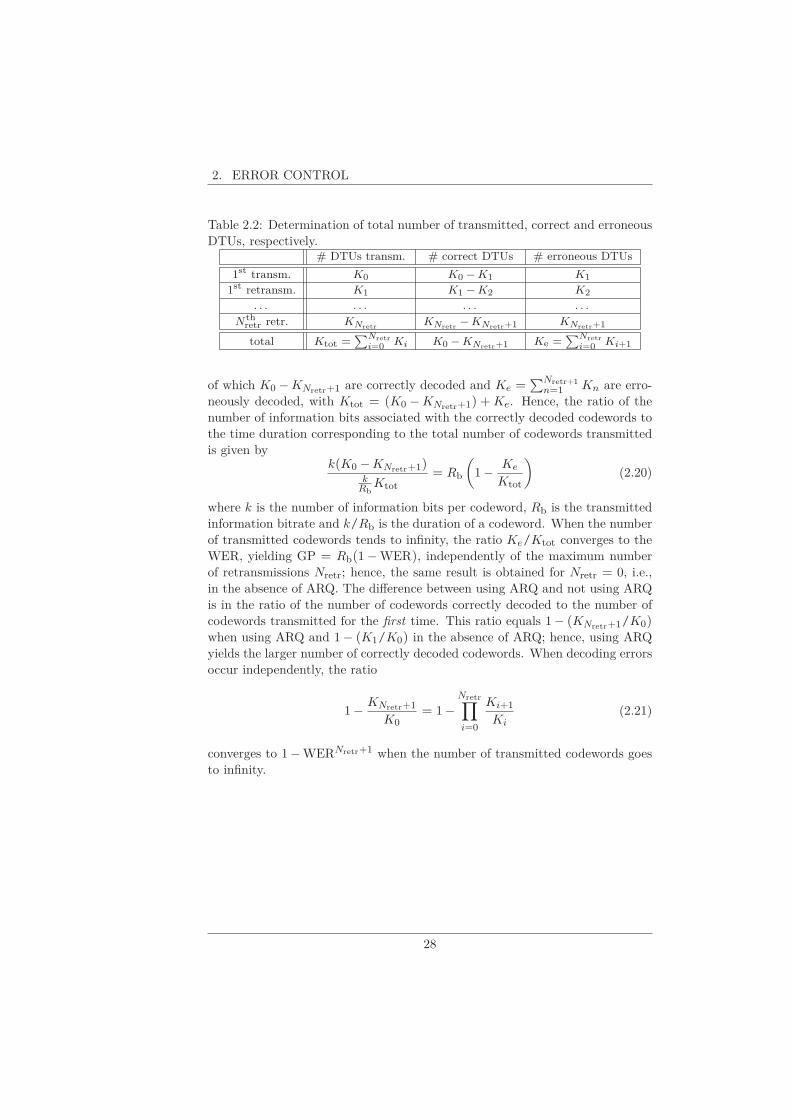
2. ERROR CONTROL
Table 2.2: Determination of total number of transmitted, correct and erroneousDTUs, respectively.
# DTUs transm. # correct DTUs # erroneous DTUs
1st transm. K0 K0 − K1 K1
1st retransm. K1 K1 − K2 K2
. . . . . . . . . . . .
Nthretr retr. KNretr
KNretr− KNretr+1 KNretr+1
total Ktot =∑
Nretr
i=0Ki K0 − KNretr+1 Ke =
∑Nretr
i=0Ki+1
of which K0 − KNretr+1 are correctly decoded and Ke =∑Nretr+1
n=1 Kn are erro-neously decoded, with Ktot = (K0 − KNretr+1) + Ke. Hence, the ratio of thenumber of information bits associated with the correctly decoded codewords tothe time duration corresponding to the total number of codewords transmittedis given by
k(K0 − KNretr+1)k
RbKtot
= Rb
(
1− Ke
Ktot
)
(2.20)
where k is the number of information bits per codeword, Rb is the transmittedinformation bitrate and k/Rb is the duration of a codeword. When the numberof transmitted codewords tends to infinity, the ratio Ke/Ktot converges to theWER, yielding GP = Rb(1−WER), independently of the maximum numberof retransmissions Nretr; hence, the same result is obtained for Nretr = 0, i.e.,in the absence of ARQ. The difference between using ARQ and not using ARQis in the ratio of the number of codewords correctly decoded to the number ofcodewords transmitted for the first time. This ratio equals 1− (KNretr+1/K0)when using ARQ and 1− (K1/K0) in the absence of ARQ; hence, using ARQyields the larger number of correctly decoded codewords. When decoding errorsoccur independently, the ratio
1− KNretr+1
K0= 1−
Nretr∏
i=0
Ki+1
Ki(2.21)
converges to 1−WERNretr+1 when the number of transmitted codewords goesto infinity.
28

Part I
Transmission over the DSL
Channel
29

3Introduction to DSL Com-munication
This chapter gives an introduction on the transmission over Digital SubscriberLine (DSL) channels. We provide in Section 3.1 a brief history about its originand evolution. The transmission over DSL channel is prone to noise ingress suchas crosstalk and impulsive noise. In Sections 3.2 and 3.3, we explain how thesenoise sources arise, and which actions are taken to maintain a good performance.
3.1 History
In this dissertation, our algorithms and protection strategies are applied toa recent DSL technology, called Fast Access to Subscriber Terminals or G.fast.This G.fast technology has been preceded by a whole series of DSL technologies,of which we present here a brief history.
DSL stands for a group of technologies that are commonly used to providebroadband internet access by transmitting digital data over telephone lines [28].The public switched telephone netword (PSTN) was originally designed to carryvoice signals. Each home is connected to the telephone network by twisted pair,invented by Alexander Graham Bell. Twisted pair consists of two isolated copper
31

3. INTRODUCTION TO DSL COMMUNICATION
wires which are twisted to reduce interference from external noise sources. Thebandwidth of the voice signal is limited to the frequency range from 0.3 to 3.4kHz. A number of twisted pairs is bundled in a cable binder.
Figure 3.1: Alexander Graham Bell (March 3, 1847, Scotland – August 2, 1922).
The digital data is transmitted in a frequency band higher than the voiceband. At the customer premises, the data is filtered from the voice service.A general diagram of a DSL system is depicted in Figure 3.2. The DSL loopcorresponds to the twisted pair loop between the local central office and the
customer premises, and a DSL modem is required at each end of the loop. The
DSL access multiplexer (DSLAM) in the CO contains several DSL modems
serving multiple customers. The DSLAM connects the twisted pair to both the
data network and the PSTN.
We give here a brief outline of a selection of some notable DSL technologies
from the past until today:
• A precursor of DSL is integrated services digital network (ISDN), offering160 kb/s over distances up to 5.5 km [29]. The data rates are limited
due to the large near-end crosstalk (NEXT) caused between signals in
telephone lines traveling in opposite directions.
• High-bitrate digital subscriber line (HDSL) provides the symmetric bitrateof 1.544 Mbit/s to customers over two copper twisted pairs. It operates in
the baseband and it does not allow for coexistence with telephone traffic.
It is typically used to serve sites with business customers. HDSL2, a
successor of HDSL, includes TCM as error correction code to enhance
performance.
• NEXT is circumvented in asymmetric DSL (ADSL) by applying frequencydivision duplexing (FDD); the upstream and downstream frequency bands
are separated. The term ’asymmetric’ is used because of the different data
rates in upstream (low data rate up to 896 kb/s) and downstream (high
data rate up to 8 Mb/s) directions [29]. Generally, upstream transmission
uses the frequency band from 25 kHz up to 138 kHz and downstream
transmission goes from 138 kHz up to 1.1 MHz.
32

3.1. HISTORY
CO
DSLAM
DSL
modem
PSTN
data
network
twisted pair
DS
CO
Figure 3.2: Generic DSL architecture block diagram.
In the 1990s, discrete multitone transmission (DMT) was proposed byJohn Cioffi, known as ’the father of DSL’. DMT transmission refers toa multi-carrier system with variable constellation sizes that makes DSL
highly adaptive to the variation in loop length and external noise sources.
Multi-carrier systems partition the available bandwidth into a (large) num-
ber of subchannels, called tones; each tone supports a number of bits de-
pending on its SNR and the desired bit error probability. During each
DMT symbol period, a multi-carrier signal is transmitted, which contains
one constellation symbol per tone. More details about DMT transmission
are given in Section 4.1.
Figure 3.3: John Cioffi (November 7, 1956, Illinois).
• Very-high bit rate DSL (VDSL) uses a bandwidth up to 12 MHz. As signalattenuation increases with frequency, the distances that can be covered
become shorter. The network is upgraded by introducing optical fiber.
The resulting network architecture consists of a fiber link between the
33

3. INTRODUCTION TO DSL COMMUNICATION
central office and a optical network unit in the street, needed to convert the
optical signal to an electrical signal. The remaining distance (typically less
than 1 km) to the customer premises is covered using VDSL transmission
over twisted copper pair. Due to this hybrid fiber-copper connection with
the central office, the length of the copper loops is shortened and higher
bit rates are achieved (up to 52 Mb/s downstream and 6.4 Mb/s upstream
transmission for a 300 m loop). Thanks to these higher speeds, VDSL is
able to support capacity-demanding applications such as HDTV.
• VDSL2 is currently the highest-speed DSL variant available and uses thefrequency band up to 30 MHz on loop lengths similar to those used with
VDSL [5]. A signal coordination technique called vectoring can be used to
cancel the far-end crosstalk (FEXT), caused by signals on telephone lines
traveling in the same direction. VDSL2 typically achieves a throughput
of 30-40 Mb/s in the presence of crosstalk, which is increased beyond 100
Mb/s if the crosstalk is removed by vectoring [30, 31]. The VDSL2-based
DMT modulation uses for frequencies up to 12 MHz, a tone spacing of
4.3125 kHz and a DMT symbol rate of 4000 symbols/s. For frequencies
up to 30 MHz, a tone spacing of 8.625 kHz is used and a DMT symbol
rate of 8000 symbols/s.
Users continue to increase the bit rate demand for many different applications.
As the core network mainly consists of fiber, the twisted pair access network
to the core network has become a bottleneck that limits the available data
rates, as the fiber network has a capacity far beyond the capacity of the copper
network [32]. The ultimate goal is fiber access for every user, also called fiber-to-
the-home (FTTH). The bandwidth offered by FTTH would be enough to even
satisfy the most demanding user. But the cost of the installation is considerable;
the twisted pair access network is the major part of the installed network and
replacing it with fiber is very expensive. A full FTTH network will not be
achieved in the near future, the investments are rather spread over a longer
time period. Therefore, internet service providers expressed interest to further
boost the capacity of copper access networks to enable fiber-like speeds without
full FTTH deployment.
• Fast Access to Subscriber Terminals (G.fast), is a copper technology forfiber-to-the-distribution-point (FTTdp) deployments with copper loops of
30 m to 250 m, targeting a 1 Gb/s downstream bitrate on very short loops
and several hundred Mb/s for longer loops (e.g., 500 Mb/s and 200 Mb/s
on 100 m and 200 m, respectively) [33–35]. Optical fiber connects the
central office with distribution points in street cabinets or basements of
buildings, located very close to the user as visualized in Figure 3.4.
The existing copper telephone wiring provides the connection from the
distribution points to the homes. This FTTdp architecture is continuing
34

3.2. CROSSTALK AND PRECODING
Figure 3.4: FTTdp architecture with a fiber core network and a twisted pairaccess network.
the gradual deployment of fiber, making the fiber termination move closerto the home, and hence reducing the length of the twisted pair segment.On short DSL loops, higher bit rates can be achieved through higher signalbandwidths, because signal attenuation increases less with frequency ascompared to longer loops.
The G.fast-based DMT modulation uses frequencies up to 212 MHz, atone spacing of 51.75 kHz and a DMT symbol rate of 48000 symbols/s. Itcarries up to 12 (coded) bits per tone in the DMT symbol. As opposed toprevious DSL technologies, G.fast uses time division duplexing (TDD) toseparate downstream and upstream traffic.
In the next chapters of this first part of the dissertation, we will apply our
results and algorithms to this type of channel.
3.2 Crosstalk and Precoding
As multiple copper pairs are usually bundled in binders, the transmission suffers
from crosstalk among twisted pairs. Crosstalk is the primary noise source in
DSL systems [29]. Vectoring can substantially cancel the crosstalk by means
of proper signal coordination [36]. In downstream communications, the trans-
mitting modems are co-located in the same distribution point, allowing for the
joint processing of the signals before transmission. The customer premises of
the end users are geographically separated, which makes joint processing of the
received signals infeasible. Before transmission, the signals are precoded in such
35

3. INTRODUCTION TO DSL COMMUNICATION
a way that the combination of the precoding and crosstalk cancels out. Theresulting gain can be significant; e.g., VDSL2 typically achieves a throughputof 30-40 Mb/s in the presence of crosstalk; this throughput is increased beyond100 Mb/s if the crosstalk is canceled by means of precoding [30,31].
In the case of linear precoding (LP), the columns of the precoding matrix aremade proportional to the columns of the inverse of the channel matrix. In thespectrum range of VDSL2, which is limited to 30 MHz, the channel matrix andthe corresponding precoder are diagonally dominant, in which case the linearprecoder is near-optimal in terms of data rate [37]. However, as in G.fast thespectrum band goes up to 212 MHz, the channel matrix is no longer diagonallydominant [38]; in this case the large off-diagonal elements of the linear precodingmatrix (i.e. the additional power used by the crosstalk precompensation signals)increase the transmit power spectral density (PSD), hence deteriorating theresulting data rate under a given transmit PSD constraint. This problem can becircumvented by using nonlinear precoding (NLP), which reduces the transmitPSD as compared to LP by introducing a modulo operation at the transmittingside [36]; however, NLP requires also a modulo operation to be applied at thereceiving side, which to some extent degrades the error performance of thereceiver since the modulo operation creates additional nearest neighbours forthe outer constellation points. This will be elaborated in Chapter 4.
3.3 Impulsive Noise
Impulsive noise (IN) manifests itself as occasional short noise pulses of significantenergy. This type of noise is typically caused by electrical power switchingoriginating from human activity near the user’s premises. E.g., the switching ofa fluorescent lamp, an electrical traction motor like used in trams, trains andtrolley buses, telephone ringing... Also weather conditions such as lightningcan cause the occurrence of IN. The shape, duration, energy and inter arrivaltime of the pulses vary widely. There is no commonly accepted model for thenoise impulses, in this dissertation we will use a simple model, the parametersof which are fitted to the experimental data reported in [39] and [40].
The reduction of the DMT symbol duration in G.fast increases the vulner-ability to impulsive noise as compared to VDSL2, because an individual noiseimpulse is likely to hit consecutive DMT symbols in G.fast. Error-control tech-niques that have proven useful for long DMT symbols (as used in VDSL2)might be inadequate for short DMT symbols. This motivates the investigationof error-control techniques for short DSL loops.
When using a static configuration of error correcting codes to cope withnon stationary impulsive noise, the coding must be dimensioned to handle largenoise levels that occur only occasionally, thereby introducing a large parityoverhead and/or a large interleaving delay. This can be avoided by using anadaptive error-control protocol such as a retransmission protocol (automatic
36

3.3. IMPULSIVE NOISE
repeat request (ARQ) protocol). ARQ enables the receiver to request the re-transmission of a packet or data transfer unit (DTU) that has been erroneouslyreceived. With ARQ, the additional overhead and latency caused by retransmis-sions occur only when the noise level occasionally exceeds the error correctingcapability of the code. For a VDSL2 system with frequencies used up to 17MHz and TDMT = 250 µs, it has been shown in [41] that using ARQ instead ofinterleaving can considerably reduce the latency.
The reader is referred to Section 4.5 for more information about the statis-tical model used for the IN.
37

3. INTRODUCTION TO DSL COMMUNICATION
38

4DSL System Description
In this chapter, we describe the system model as it is used throughout the firstpart of this dissertation about the transmission over the DSL channel. Section4.1 provides a mathematical description of the communication over the channelthat suffers from crosstalk. Section 4.2 gives an overview of the constellationtypes used. The crosstalk in DSL transmission is tackled by means of precod-ing. Section 4.3 addresses linear precoding (LP), which is adequate in moderatecrosstalk environments. When the crosstalk is strong, we might require nonlin-ear precoding (NLP), which is presented in Section 4.4. Section 4.5 provides astatistical model for the impulsive noise.
4.1 DSL Channel Model
We consider the downlink transmission from a distribution point (DP) to Nu
users at different locations; each user is connected to the DP by means of atwisted pair cable. Denoting by xi(t) and yi(t) the signals transmitted and
39
4. DSL SYSTEM DESCRIPTION
received on the ith twisted pair cable (i = 1, ...,Nu), we have
yi(t) =Nu∑
j=1
∫
hi,j(t − u)xj(u)du + ni(t) (4.1)
where hi,j(t) is the impulse response from the input of the jth cable to theoutput of the ith cable, and ni(t) represents stationary Gaussian noise1; thenoise terms corresponding to different user indices are statistically independent.The impulse responses hi,i(t) correspond to the direct channels, whereas theimpulse responses hi,j(t) with j Ó= i denote the crosstalk channels. We assumecausal impulse responses with a finite duration not exceeding Tch, i.e., hi,j(t) = 0
for t < 0 and for t > Tch.The Nu transmitters at the DP make use of discrete multitone (DMT) mod-
ulation which includes a cyclic prefix to avoid interference between successiveDMT symbols. Basically, the signal xi(t) consists of blocks of duration TDMT;these blocks are referred to as DMT symbols. During the lth DMT symbol, a
vector xi(l) =(
x(1)i (l), ...,x
(Nt)i (l)
)
of Nt zero-mean uncorrelated components
is transmitted, with each component modulating a different subcarrier or tone.The frequencies of the Nt tones are multiples of a frequency spacing F . Thequantities TDMT and F are related by TDMT = TCP + 1
F , with TCP > Tch;typically, we select F such that TCPF ≪ 1 (in G.fast, we have TDMT = 1/48000s = 20.833 µs and F = 51.75 kHz, so that TCP = 1.510 µs and TCPF = 0.078).The real-valued transmit signal during the lth DMT symbol interval is given by
xi(t) =
√2
TDMT
Nt∑
k=1
ℜ(
x(k)i (l)ej2πkF t
)
t ∈ [lTDMT, (l + 1)TDMT) (4.2)
with kF denoting the frequency of the kth tone. As the signal segments in theintervals t ∈ [lTDMT, lTDMT + TCP) and t ∈ [(l + 1)TDMT − TCP, (l + 1)TDMT)are identical, the first segment of duration TCP is referred to as the cyclic prefixof the DMT symbol.
The normalization factor√
2TDMT
in (4.2) ensures that the transmit energy
on the kth tone during the lth DMT symbol equals E[|x(k)i (l)|2]. Assuming that
E[|x(k)i (l)|2] does not depend on the DMT symbol index l, the transmit power
associated with the kth tone equals E[|x(k)i |2]/TDMT, and the aggregate transmit
power (sum over all tones) on the ith cable equals∑Nt
k=1 E[|x(k)i |2]/TDMT. The
(two-sided) power spectral density Sxi(f) of xi(t) is given by
Sxi(f) =
1
2
Nt∑
k=1
E[|x(k)i |2] (S(f − kF ) + S(k + F )) (4.3)
1The occurrence of impulsive noise will be considered in Section 4.5.
40

4.1. DSL CHANNEL MODEL
where
S(f) =
(sin(πfTDMT)
πfTDMT
)2
is concentrated near f = 0, and has a mainlobe width of 2/TDMT. Taking intoaccount that TCPF ≪ 1 yields S(mF ) ≪ S(0) for any nonzero integer m, it
follows that Sxi(kF ) = Sxi
(−kF ) ≈ 12E[|x(k)
i |2]. Hence, the one-sided powerspectral density (defined as 2Sxi
(f) for f ≥ 0 and zero otherwise) at f = kF is
accurately approximated by E[|x(k)i |2].
The response yi,j(t) of the ith cable to the transmitted DMT signal xj(t) isobtained by convolving xj(t) with the impulse response hi,j(t). At the receiver,the cyclic prefix of each DMT symbol is discarded, and only the remaining part(of duration 1
F ) of each DMT symbol is processed; hence, the useful part of thelth DMT symbol at the receiver is obtained as
yi,j(t) =
∫
hi,j(t − u)xj(u)du t ∈ [lTDMT + TCP, (l + 1)TDMT) (4.4)
Because of discarding the cyclic prefix at the receiver, the transmitted DMTsymbols having an index less than l do not contribute to yi,j(t) in (4.4) dur-ing the considered interval; similarly, transmitted DMT symbols with an in-dex larger than l do not contribute either, because the impulse responses arecausal. Hence, only the lth transmitted DMT symbol must be taken into ac-count, so that the integration in (4.4) can be restricted to the interval u ∈[lTDMT, (l + 1)TDMT). As the duration of hi,j(t) is less than TCP, (4.4) can betransformed into
yi,j(t) =
√2
TDMT
Nt∑
k=1
ℜ(
Hi,j(kF )x(k)j (l)ej2πkF t
)
t ∈ [lTDMT+TCP, (l+ 1)TDMT)
(4.5)where Hi.j(f) is the Fourier transform of hi,j(t). The received signal yi(t)during the useful part of the lth DMT symbol is then obtained as
yi(t) =Nu∑
j=1
yi,j(t) + ni(t) (4.6)
where yi,j(t) is given by (4.5).The receiver performs a demodulation according to
y(k)i (l) =
√
2TDMTF
(l+1)TDMT∫
lTDMT+TCP
yi(t)e−j2πkF tdt (4.7)
Taking into account that F∫
1/Fej2πmF tdt = δm with δm denoting the Kro-
41

4. DSL SYSTEM DESCRIPTION
necker delta function, we obtain
y(k)i (l) =
Nu∑
j=1
Hi,j(kF )x(k)j (l) + n
(k)i (l) (4.8)
Considering that ni(t) is zero-mean stationary Gaussian noise with (two-sided)
power spectral density Sni(f), the complex random variables n
(k)i (l) are zero-
mean Gaussian and circular symmetric with E
[
n(k)i (l)
(
n(k′)i (l)
)∗]
= N(k)0,i δk−k′ ,
where N(k)0,i = 2(1+ TCPF )Sni
(kF ). Hence, the noise contributions n(k)i (l) are
independent across tones, with variances N(k)0,i . When ni(t) is white Gaussian
noise, Sni(f) does not depend on f , so that N
(k)0,i becomes independent of the
tone index k (and will be denoted N0,i; in this case, the noise contributions
n(k)i (l) are i.i.d. across tones, with variance N0,i).As there is no interference between consecutive DMT symbols, we will drop
the DMT symbol index for notational convenience. The resulting observationmodel can be compactly represented as
y(k) = H(k)x(k) + n(k) (4.9)
where the superscript k refers to the tone index (k = 1, ...,Nt), the received vec-tor y(k), the transmitted vector x(k) and the noise vector n(k) have dimensionNu × 1, and the channel matrix H(k) has dimension Nu × Nu. The ith compo-nents (i = 1, ...,Nu) of the vectors x(k), y(k) and n(k) represent the quantities
x(k)i , y
(k)i and n
(k)i , respectively. The element H
(k)i,j ofH(k) equals Hi,j(kF ). The
components of n(k) are zero-mean statistically independent circular symmetric
Gaussian random variables with E
[
|n(k)i |2
]
= N(k)0,i .
In a practical implementation, the modulation (4.2) is replaced by first ob-taining the N -point IFFT of the vector
(
0,x(1)i (l), ...,x
(Nt)i (l), 0, ...0,
(
x(Nt)i (l)
)∗, ...,
(
x(1)i (l)
)∗)
consisting of a zero, the Nt constellation symbol values of the considered DMTsymbol, N − 2Nt − 1 zeroes, and the complex conjugates of the Nt constellationsymbol values in reversed order (implying that N must satisfy the inequalityN ≥ 2Nt + 1). Next, a vector of N + ν samples is constructed by prepending thelast ν samples of the IFFT to the beginning of the IFFT, and finally these N + ν
samples are applied at a rate 1/T to a transmit filter. The sampling intervalT satisfies T = 1/(NF ) with F denoting the tone spacing, and ν should beselected such that νT > Tch; the resulting durations of the DMT symbol andthe cyclic prefix are TDMT = (N + ν)T and TCP = νT , respectively. Thedemodulation operation (4.7) is replaced by applying yi(t) to a receive filter,sampling the receiver filter output at the rate 1/T , keeping the N samples that
42

4.2. CONSTELLATION TYPES
correspond to the useful part of the considered DMT symbol, and performingan N -point FFT on these samples. Typically, N is an integer power of 2. Theresulting observation model can again be represented by (4.9).
Each of the Nu transmit signals is subject to a maximum power spectraldensity (PSD) and a maximum aggregate transmission power (ATP) constraintper line. These constraints translate into
E
[
|x(k)i |2
]
≤ E(k)PSD all (i, k) (4.10)
Nt∑
k=1
E
[
|x(k)i |2
]
≤ EATP all i (4.11)
where E(k)PSD is the maximum one-sided PSD at frequency kF , and EATP =
PATP/TDMT, with PATP denoting the maximum aggregate transmit power.
4.2 Constellation Types
The information bit sequences to be sent to the Nu users are (possibly) encodedfor increased robustness against transmission errors, and the resulting coded bitsare mapped to constellation symbols. The constellation symbol for the ith user
sent on the kth tone is denoted a(k)i , and belongs to a constellation A(k)
i with
M(k)i = 2b
(k)i points. For mathematical convenience, we consider normalized
constellations, i.e., the constellation symbols have unit energy: E[|a(k)i |2] = 1;
a non-normalized constellation symbol with energy E(k)i is then denoted as
√
E(k)i a
(k)i . The number of points in the constellations A(k)
i and the constella-
tion symbol energies E(k)i are design parameters. For further use, we introduce
the Nu × 1 vector a(k), the ith component of which equals a(k)i (i = 1, ...,Nu)
and the Nu × Nu diagonal matrix E(k) with(
E(k))
i,i= E
(k)i ; the vector of
non-normalized symbols is then given by(
E(k))1/2
a(k).
If we simply set x(k)i =
√
E(k)i a
(k)i , the users would suffer from crosstalk,
because of the nonzero off-diagonal elements of the channel matrix H(k) from(4.9). As the users are at different locations, they cannot cooperate to cancel thisinterference. Therefore, we allow the Nu transmitters at the DP to cooperate inorder to avoid interference at the users’ receivers. This transmitter-side signal
coordination (or vectoring) is referred to as precoding; the corresponding x(k)i
is a function of a(k) rather than only a(k)i .
We restrict our attention to quadrature amplitude modulation (QAM) con-stellations CM containing M = 2b points, with b ∈ {1, 2, ..., bmax}; b representsthe number of coded bits per constellation symbol. The real and imaginary
43

4. DSL SYSTEM DESCRIPTION
D+
D- D+ D+ 3
D+ 3
D-
D-3
D-3
D-
D+
D- D+
Figure 4.1: Constellations for 4-QAM and 16-QAM.
parts of the constellation points are odd multiples of the quantity ∆. Now wediscuss the different QAM constellations in more detail.
4.2.1 Square-QAM
A square-QAM constellation consists of M = 2b points, where b is an eveninteger. The set of constellation symbols for the M -QAM constellation (M = 2b)is given by CM = {((2m + 1) + j(2n + 1))∆;m,n ∈ {−
√M/2, . . . ,
√M/2−
1}}, with minimum distance d between constellation points given by d = 2∆.The average energy per symbol associated with this constellation is equal to
EM =1
M
∑
a∈CM
|a|2
=2
3(M − 1)∆
2 (4.12)
For a normalized constellation, we have EM = 1, yielding
d2 =6
M − 1(4.13)
Figure 4.1 shows the constellations for 4-QAM (b = 2) and 16-QAM (b = 4).
4.2.2 Cross-QAM
A cross-QAM constellation consists of M = 2b points, where b is an odd integerlarger than 3. The set of constellation points for the 2b-QAM constellation isgiven by CM = CM ,1 ∪ CM ,2 ∪ CM ,3 with
44

4.2. CONSTELLATION TYPES
D+ 3
D+
D- D+ D+ 3
D-
D-3
D-3D- 5 D+ 5
D+ 5
D- 5
CM,3
CM,1
CM,2
Figure 4.2: Constellation for 32-QAM.
CM ,1 = {((2m + 1) + j(2n + 1))∆;
m ∈ {−3
4M ′, . . . ,
3
4M ′ − 1},n ∈ {−1
2M ′, . . . ,
1
2M ′ − 1}}
CM ,2 = {((2m + 1) + j(2n + 1))∆;
m ∈ {−1
2M ′, . . . ,
1
2M ′ − 1},n ∈ {−3
4M ′, . . . ,−1
2M ′ − 1}}
CM ,3 = {((2m + 1) + j(2n + 1))∆;
m ∈ {−1
2M ′, . . . ,
1
2M ′ − 1},n ∈ {1
2M ′, . . . ,
3
4M ′ − 1}}
where we have set M ′ =√
M2 for conciseness; these constellations are referred
to as cross-QAM. The minimum distance d between constellation points is givenby d = 2∆. For the average energy per symbol we obtain
EM =2
3
(31
32M − 1
)
∆2 (4.14)
For a normalized constellation, we have EM = 1, yielding
d2 =6
3132M − 1
(4.15)
Figure 4.2 shows the 32-QAM constellation (b = 5).
45

4. DSL SYSTEM DESCRIPTION
D+
D-
D- D+
Figure 4.3: Constellation for 2-QAM.
D+
D- D+ D+ 3
D+ 3
D-
D-3
D-3
D+
D- D+ D+ 3
D+ 3
D-
D-3
D-3
Figure 4.4: Two types of 8-QAM constellations: 8-QAM-VDSL (left) and 8-QAM-G.fast (right).
4.2.3 2-QAM
The 2-QAM constellation (b = 1) is shown in Figure 4.3, with C2 = {(1 +j)∆,−(1+ j)∆}. The minimum distance d between constellation points is givenby d = 2
√2∆. For the average energy per symbol, we obtain
E2 = 2∆2 (4.16)
For a normalized constellation, we have E2 = 1, yielding d2 = 4.
4.2.4 8-QAM
We consider two types of 8-QAM constellations, referred to as 8-QAM-VDSLand 8-QAM-G.fast, which are shown in Figure 4.4.
The 8-QAM-VDSL constellation is part of the DSL standards since the intro-duction of DMT transmission in ADSL and still used in the VDSL standard [5].The minimum distance d between constellation points is equal to d = 2∆. Forthe average energy per symbol, we obtain
E8,VDSL = 6∆2 (4.17)
For a normalized constellation, we have E8,VDSL = 1, yielding d2 = 2/3.
46

4.3. LINEAR PRECODING
( )kQ
( )( ) ( )kkaE
2/1 ( )k'x
( )kH
( )kn
( )ky( )k
x ( )kz
( )kB-
( )kT
Figure 4.5: Block diagram of the system with linear precoder.
The 8-QAM-G.fast constellation has been proposed for the G.fast standard[42]. The minimum distance d between constellation points is equal to d =2√2∆. For the average energy per symbol, we obtain
E8,G.fast = 10∆2 (4.18)
For a normalized constellation, we have E8,G.fast = 1, yielding d2 = 4/5.
4.3 Linear Precoding
4.3.1 Derivation of Linear Precoding Structure
In the case of linear precoding (LP), we counteract the crosstalk generated bythe off-diagonal elements of H(k) by applying at the transmitter a linear trans-
formation to the non-normalized constellation symbol vector(
E(k))1/2
a(k),
i.e., the transmit vector x(k) is given by x(k) = P(k)(
E(k))1/2
a(k), where P(k)
is a Nu × Nu precoding matrix.We select the precoding matrix P(k) such that the crosstalk is completely
canceled at the users’ receivers; this is referred to as zero-forcing (ZF) linear pre-
coding. First we consider the QR decomposition of(
H(k))H
, i.e.,(
H(k))H
=
Q(k)R(k), where Q(k) is a unitary matrix ((
Q(k))H
Q(k) = Q(k)(
Q(k))H
= I)
and R(k) is an upper triangular matrix. From this, we obtain the following
decomposition of H(k): H(k) = L(k)(
Q(k))H
, with L(k) =(
R(k))H
denoting
a lower triangular matrix. Next, we decompose L(k) as L(k) = D(k)L
(I+B(k)),
where D(k)L
is a diagonal matrix with(
D(k)L
)
i,i= L
(k)i,i , I denotes the identity
matrix, and B(k) is a lower triangular matrix with zeroes on its diagonal. This
yields H(k) = D(k)L
(I+B(k))(
Q(k))H
. Now we select the precoding matrix as
47

4. DSL SYSTEM DESCRIPTION
P(k) = Q(k)(I+B(k))−1; this gives rise to H(k)P(k) = D(k)L, which indicates
that the cascade of the precoder P(k) and the channel H(k) acts as a diagonal
channel matrix D(k)L, so that crosstalk is indeed eliminated.
Because of the particular structure of the precoding matrix, the trans-mit vector can be represented as x(k) = Q(k)x′(k), with (I + B(k))x′(k) =(
E(k))1/2
a(k). Considering that B(k) is lower triangular with zero diagonal,
the elements of x′(k) can be computed recursively as follows:
x′(k)1 =
√
E(k)1 a
(k)1 (4.19)
x′(k)i =
√
E(k)i a
(k)i −
i−1∑
j=1
B(k)i,j x
′(k)j (i > 1) (4.20)
The resulting system with linear precoding is shown in Figure 4.5.At the input of the receiver of the ith user we obtain
y(k)i = L
(k)i,i
√
E(k)i a
(k)i + n
(k)i (4.21)
The symbol energy E(k)i is a design parameter, which should be selected such
that the resulting E
[
|x(k)i |2
]
satisfy the constraints (4.10) and (4.11). De-
fine N(k)0 as the diagonal matrix with
(
N(k)0
)
i,i= N
(k)0,i . For mathematical
convenience, we apply to y(k) a reversible transformation z(k) = T(k)y(k),
consisting of a rotation and a scaling of the components y(k)i , i.e., z
(k)i =
y(k)i exp(−j arg(L
(k)i,i ))/
√
N(k)0,i ; hence, T
(k) is a diagonal matrix with
(T(k))i,i = exp(−j arg(L(k)i,i ))/
√
N(k)0,i (4.22)
Because of the reversibility of the transformation, z(k) and y(k) contain the same
information about the constellation symbol vector a(k). The resulting z(k)i can
be decomposed as
z(k)i =
√
SNR(k)i a
(k)i + w
(k)i (4.23)
where
SNR(k)i =
|L(k)i,i |2E(k)
i
N(k)0,i
(4.24)
denotes the SNR on the kth tone at the input of the ith receiver, and E[|w(k)i |2] =
1.
48

4.3. LINEAR PRECODING
4.3.2 Transmit Energy
Considering that the components of a(k) are uncorrelated, the energy of thecomponents of the transmit vector x(k) = P(k)a(k) at the output of the precod-ing matrix can be computed as
E
[
|x(k)i |2
]
=Nu∑
j=1
|P (k)i,j |2E(k)
j (4.25)
Hence, in view of (4.25), when some components of the precoding matrix P(k)
have a large magnitude, some of the E(k)i should be small in order to satisfy
the constraints (4.10)-(4.11), yielding small values of the corresponding SNR(k)i ;
in this case, only small constellation sizes can be used to achieve a satisfactory
error performance at small SNR(k)i , which limits the information bitrate. This
problem can be circumvented by using nonlinear precoding, which is describedin the next section.
4.3.3 Alternative Linear Precoding Structure
An alternative formulation of the zero-forcing linear precoding involves decom-
posing the channel matrix as H(k) = D(k)H
(
I+C(k))
[36], where D(k)H
is a
diagonal matrix with(
D(k)H
)
i,i= H
(k)i,i , I denotes the identity matrix, and the
diagonal elements of C(k) are zero; the off-diagonal elements of C(k) are indica-tive of the coupling between the twisted pair cables. The precoder is selected as
P′(k) =(
I+C(k))−1
, which yieldsH(k)P′(k) = D(k)H. Denoting in this alterna-
tive formulation the non-normalized symbol related the kth tone and the ith user
as√
E′(k)i a
(k)i , it is easily verified that the original formulation and the alterna-
tive formulation are equivalent (i.e., they yield the same transmit and receivevectors x(k) and y(k), so they satisfy the same transmit power constraints and
achieve the same error performance) when√
E′(k)i =
√
E(k)i L
(k)i,i /H
(k)i,i . The
alternative system avoids the QR decomposition of(
H(k))H
, but requires the
inversion of I+C(k). In the case of small to moderate crosstalk, this inversecan be approximated by truncating the infinite series expansion
(
I+C(k))−1
=∑
l≥0(−1)l
(
C(k))l
to only a few terms, e.g.,(
I+C(k))−1
≈ I−C(k). However, such approxima-
tion is no longer accurate in the presence of strong crosstalk; moreover, whenC(k) has one or more eigenvalues with a magnitude exceeding 1, the aboveinfinite series does not converge.
49

4. DSL SYSTEM DESCRIPTION
Table 4.1: Values of d2 for the 2b-QAM constellations with b = 1, . . . , 12.
b 1 2 3 (VDSL) 3 (G.fast) 4 5 6
d2 4 2 2/3 4/5 2/5 1/5 2/21
b 7 8 9 10 11 12
d2 2/41 2/85 2/165 2/341 2/661 2/1365
4.3.4 Comparison of Different Constellations
Considering (4.23), we will show in Chapter 5 that the error performance foruncoded transmission and for TCM is mainly determined by the minimum dis-
tance between the scaled constellation symbols√
SNR(k)i a
(k)i , with a
(k)i ∈ A(k)
i ;
this distance equals√
SNR(k)i d
(k)i , where d
(k)i is the minimum distance of the
normalized constellation A(k)i . For a given channel matrix H(k), let us replace
for all (i, k) the normalized constellations A(k)i (with minimum distance d
(k)i )
and the symbol energies E(k)i by the normalized constellations A′(k)
i (with min-
imum distance d′(k)i ) and the symbol energies E
′(k)i . In order that the transmit-
ted energies E
[
|x(k)i |2
]
from (4.25) remain the same, we select E′(k)i = E
(k)i ,
yielding SNR′(k)i = SNR
(k)i (see (4.24)). Hence, compared to the constellation
A(k)i scaled by the factor
√
SNR(k)i , the minimum distance associated with the
constellation A′(k)i scaled by the factor
√
SNR′(k)i is increased by the factor
d′(k)i /d
(k)i . Table 4.1 summarizes the values of d2 for the various constellations.
Comparing 8-QAM-VDSL (with d2 = 2/3) and 8-QAM-G.fast (with d2 = 4/5),it follows that the latter has an advantage of 10 log(6/5) = 0.79 dB over theformer, in terms of Euclidean distance of the scaled constellations.
4.4 Nonlinear Precoding
4.4.1 Derivation of Nonlinear Precoding Structure
We consider zero-forcing nonlinear precoding (NLP) of the Tomlinson-Harashimatype [36]. This type of precoding makes use of modulo operations at the trans-mitter.
For any real-valued u and any positive divisor A, we define u modulo A
as [u]A = u + lA, where l is the unique integer such that −A/2 ≤ u + lA <
A/2. This definition is easily extended to complex-valued u, by defining [u]A =[ℜ(u)]A + j[ℑ(u)]A. For α > 0, we have the relation [αu]αA = α[u]A. The
50

4.4. NONLINEAR PRECODING
( )kQ
( )( ) ( )kkaE
2/1 ( )k'x
( )kH
( )kn
( )ky( )k
x( )kz
( )kB-
[ ] ( )( ) ( )kkAE
2/1 ( )kT
Figure 4.6: Block diagram of the system with nonlinear precoder.
modulo operation on a complex-valued vector u corresponds to the component-wise application of the modulo operation; denoting by Ai the divisor related toui, the ith component of u, we have ([u]A)i = [ui]Ai
, with (A)i = Ai.The only difference between the nonlinear precoder and the linear precoder
from Figure 4.5 is in the way x′(k) is obtained. In the case of NLP, we have
x′(k)1 =
[√
E(k)1 a
(k)1
]
√
E(k)1
A(k)1
(4.26)
x′(k)i =
√
E(k)i a
(k)i −
i−1∑
j=1
B(k)i,j x
′(k)j
√
E(k)i
A(k)i
(i > 1) (4.27)
The selection of the quantity A(k)i will be discussed shortly. Because of the mod-
ulo operation, the real and imaginary parts of x′(k)i have a magnitude not ex-
ceeding√
E(k)i A
(k)i /2, which indicates that the value of A
(k)i affects E[|x′(k)
i |2].Alternatively, x
′(k)i can be represented as
x′(k)1 =
√
E(k)1
(
a(k)1 + l
(k)1 A
(k)1
)
(4.28)
x′(k)i =
√
E(k)i
(
a(k)i + l
(k)i A
(k)i
)
−i−1∑
j=1
B(k)i,j x
′(k)j (i > 1) (4.29)
where l(k)i = l
(k)R,i + jl
(k)I,i , and l
(k)R,i and l
(k)I,i are the unique integers such that
the real and imaginary parts of the right-hand sides of (4.28) and (4.29) are
in the interval
[
−√
E(k)i A
(k)i /2,
√
E(k)i A
(k)i /2
)
. Considering the similarity be-
tween (4.28)-(4.29) and (4.19)-(4.20), it follows that the receive vector y(k) is
51

4. DSL SYSTEM DESCRIPTION
determined by
y(k)i = L
(k)i,i
√
E(k)i
(
a(k)i + l
(k)i A
(k)i
)
+ n(k)i (4.30)
Applying to y(k) the same transformation matrix T(k) as in the case of LPyields z(k) = T(k)y(k), with
z(k)i =
√
SNR(k)i
(
a(k)i + l
(k)i A
(k)i
)
+ w(k)i (4.31)
where SNR(k)i is given by (4.24) and E[|w(k)
i |2] = 1. The corresponding systemwith NLP is shown in Figure 4.6.
4.4.2 Selection of A(k)i
When a(k)i belongs to an M
(k)i -QAM constellation A(k)
i , then a(k)i + l
(k)i A
(k)i be-
longs to a periodically extended M(k)i -QAM constellation (extension with period
A(k)i in the horizontal and vertical directions), which we denote as A(k)
ext,i. The
value of A(k)i affects the Euclidean distance between points of the constellation
A(k)ext,i. We take the smallest A
(k)i for which the minimum Euclidean distance
in A(k)ext,i is the largest possible, i.e., equal to the minimum Euclidean distance
in the original constellation A(k)i . A larger A
(k)i would maintain the minimum
Euclidean distance in A(k)ext,i, but yield an increase of E[|x′(k)
i |2] and of the re-
sulting transmit power. When M(k)i = M = 2b, we take A
(k)i = A, according
to
A =
4∆ b = 1
8∆ b = 3 (VDSL,G.fast)
2√
M∆ square
3√
M2 ∆ cross
(4.32)
which is illustrated in Figures 4.7-4.11 for the different constellation types. Notethat the 2b-QAM constellations are enclosed by a square with side A from (4.32),so that in (4.26) the modulo operation can be dropped and, equivalently, in
(4.28) we have l(k)1 = 0.
4.4.3 Transmit Energy
For given k, the quantities x′(k)i are well approximated as independent random
variables which, for i > 1, are uniformly distributed inside a square with side√
E(k)i A
(k)i [36]. This yields
E
[
|x(k)i |2
]
=Nu∑
j=1
|Q(k)i,j |2E
[
|x′(k)j |2
]
52

4.4. NONLINEAR PRECODING
D+ 3
D+
D- D+ D+ 3
D-
D-3
D-3D- 5 D+ 5
D+ 5
D- 5
Figure 4.7: Illustration of the modulo operation for 2-QAM.
where
E
[
|x′(k)i |2
]
=
{
E(k)1 i = 1
ρ(k)i E
(k)i i > 1
(4.33)
and ρ(k)i =
(
A(k)i
)2/6. When M
(k)i = M = 2b, we obtain ρ
(k)i = ρ, with
ρ =
43 b = 1169 b = 3,VDSL1615 b = 3,G.fast
MM−1 square98
M3132
M−1 cross
(4.34)
The factor ρ(k)i is the ratio of the energy of x
′(k)i to the energy of
√
E(k)i a
(k)i ; we
note from (4.34) that the maximum value of this ratio amounts to 16/9 (2.5 dB),which occurs for 8-QAM-VDSL. For square and cross constellations, ρ decreaseswith increasing M , and converges to 1 (0 dB) and 36/31 (0.65 dB), respectively.
4.4.4 Comparison of Constellations
Considering (4.31), we will show in Chapter 5 that the error performancefor uncoded transmission and for TCM is mainly determined by the mini-
mum distance between the scaled constellation symbols√
SNR(k)i a
(k)i , with
a(k)i ∈ A(k)
i ; this distance equals√
SNR(k)i d
(k)i , where d
(k)i is the minimum
distance of the normalized constellation A(k)i . For a given channel matrix H(k),
53

4. DSL SYSTEM DESCRIPTION
D-3
D+ 9
D+ 3
D+
D- D+ D+ 3
D-
D-3D- 5 D+ 5
D+ 5
D- 5
D-7D-9D-11
D+ 7
D+11
D+ 7 D+ 9 D+11
D-7
D-9
D-11
Figure 4.8: Illustration of the modulo operation for the 8-QAM-VDSL constel-lation with A = 8∆.
54

4.4. NONLINEAR PRECODING
D-3
D+ 9
D+ 3
D+
D- D+ D+ 3
D-
D-3D- 5 D+ 5
D+ 5
D- 5
D-7D-9D-11
D+ 7
D+11
D+ 7 D+ 9 D+11
D-7
D-9
D-11
Figure 4.9: Illustration of the modulo operation for the 8-QAM-G.fast constel-lation.
55

4. DSL SYSTEM DESCRIPTION
D-3
D+ 9
D+ 3
D+
D- D+ D+ 3
D-
D-3D- 5 D+ 5
D+ 5
D- 5
D-7D-9D-11
D+ 7
D+11
D+ 7 D+ 9 D+11
D-7
D-9
D-11
Figure 4.10: Illustration of the modulo operation for square constellations.
56

4.4. NONLINEAR PRECODING
D-3
D+ 9
D+ 3
D+D- D+ D+ 3
D-
D-3D- 5 D+13
D+ 5
D- 5
D-7D-9D-11
D+ 7
D+11
D+ 7 D+ 9 D+11
D-7
D-9
D-11
D+ 5 D+15 D+17D-17 D-15 D-13
D-13
D-17
D-15
D+15
D+17
D+13
Figure 4.11: Illustration of the modulo operation for cross constellations.
57

4. DSL SYSTEM DESCRIPTION
Table 4.2: Values of d2/ρ for the 2b-QAM constellations with b = 1, . . . , 12.
b 1 2 3 (VDSL) 3 (G.fast) 4 5 6
d2/ρ 3 3/2 3/8 3/4 3/8 1/6 3/32
b 7 8 9 10 11 12
d2/ρ 1/24 3/128 1/96 3/512 1/384 3/2048
let us replace for all (i, k) the normalized constellations A(k)i (with minimum
distance d(k)i ) and the symbol energies E
(k)i by the normalized constellations
A′(k)i (with minimum distance d
′(k)i ) and the symbol energies E
′(k)i . In order
that the transmitted energies E
[
|x(k)i |2
]
from (4.33) remain the same, we select
E′(k)1 = E
(k)1 and E
′(k)i = (ρ
(k)i /ρ
′(k)i )E
(k)i for i > 0, yielding SNR
′(k)1 = SNR
(k)1
and SNR′(k)i = (ρ
(k)i /ρ
′(k)i )SNR
(k)i (see (4.24)). Hence, compared to the con-
stellation A(k)i scaled by the factor
√
SNR(k)i , the minimum distance associated
with the constellation A′(k)i scaled by the factor
√
SNR′(k)i is increased by the
factor
(
d′(k)i /
√
ρ′(k)i
)
/
(
d(k)i /
√
ρ(k)i
)
for i > 1. Table 4.2 summarizes the
values of d2/ρ for the various constellations. Comparing 8-QAM-VDSL (withd2/ρ = 3/8) and 8-QAM-G.fast (with d2/ρ = 3/4), it follows that the latterhas an advantage of 10 log(2) = 3 dB over the former in terms of Euclideandistance of the scaled constellations; this is a strong motivation to use 8-QAM-G.fast instead of 8-QAM-VDSL in the case of NLP.
Strictly speaking, for 8-QAM-VDSL, A = 6∆ (instead of A = 8∆ from(4.32)) is the smallest value that maintains d2 = 2/3 for the extended constel-lation, as shown in Figure 4.12; this yields ρ = 1 and d2/ρ = 2/3 (insteadof ρ = 16/9 and d2/ρ = 3/8) for 8-QAM-VDSL, so that the correspondingadvantage of 8-QAM-G.fast over 8-QAM-VDSL in the case of NLP becomes10log((3/4) · (3/2)) · (3/2)) = 0.51 dB (instead of 3 dB for A = 8∆). In thecase of uncoded transmission (where the error performance is determined by theminimum Euclidean distance in the extended constellation), A = 6∆ would bethe proper choice for 8-QAM-VDSL. However, for trellis-coded modulation, wewill point out in Section 5.2 that the error performance is determined by theminimum Euclidean distance in extended subsets of the original constellation.For 8-QAM-VDSL it can be verified that taking A = 6∆ actually reduces theminimum Euclidean distance in the extended subset as compared to the originalsubset; it turns out that A = 8∆ is needed in order not to reduce the distancein the extended subsets. For the other QAM constellations, the minimum valueof A (given in (4.32)) that maintains the distance in the extended constellation
58

4.4. NONLINEAR PRECODING
D-3
D+ 9
D+ 3
D+
D- D+ D+ 3
D-
D-3D- 5 D+ 5
D+ 5
D- 5
D-7D-9
D+ 7
D+ 7 D+ 9
D-7
D-9
Figure 4.12: Illustration of the modulo operation for the 8-QAM-VDSL constel-lation with A = 6∆.
59

4. DSL SYSTEM DESCRIPTION
also maintains the distance in the extended subsets.
4.5 Impulsive Noise
Accurate modeling of impulsive noise (IN) is very difficult, because IN measure-
ments made on different locations and/or at different times can show strong
variations of the IN statistics regarding pulse duration, inter-arrival times, pulse
energy and spectral content. For this reason, we will consider in this dissertation
a simple IN model with only a small number of parameters. Although simple,
the model captures the main features of IN, and, therefore, serves to assess the
robustness of various error control schemes against IN, rather than to accurately
predict system performance in an actual IN environment.
We model the IN as gated white Gaussian noise [43–45], which is switched
on and off at DMT symbol boundaries, and is added to the received signal yi(t)from (4.1). Hence, a DMT symbol is either not hit by IN, or hit by IN during the
entire DMT symbol duration; such model implies that the average duration of
a noise impulse exceeds the DMT symbol duration, which is the case in G.fast.
Taking IN into account, the demodulator output y(k)i (l) from (4.8) should be
replaced by
y(k)i (l) =
Nu∑
j=1
Hi,j(kF )x(k)j (l) + n
(k)act,i(l) (4.35)
In (4.35),
n(k)act,i(l) = n
(k)i (l) + I(l)n
(k)imp,i(l) (4.36)
denotes the instantaneous noise on the considered tone, consisting of the station-
ary noise contribution n(k)i (l) and the IN contribution I(l)n
(k)imp,i(l). We have
I(l) = 1 when the considered DMT symbol interval is hit by IN and I(l) = 0
otherwise. The quantity n(k)imp,i(l) is zero-mean Gaussian and circular symmetric
with E
[
n(k)imp,i(l)
(
n(k′)imp,i(l)
)∗]
= N0,imp,iδk−k′ ; note that the variance N0,imp,i
of n(k)imp,i(l) does not depend on the tone index k, because of the assumption
that the IN is white when present. The instantaneous variance N(k)0,act,i(l) of
n(k)act,i(l) is given by N
(k)0,act,i(l) = N
(k)0,i + I(l)N0,imp,i. The noise term n
(k)act,i(l)
is distributed according to a mixture of two zero-mean Gaussian distributions,
with variances N(k)0,i (when I(l) = 0) and N
(k)0,i + N0,imp,i (when I(l) = 1), re-
spectively; the instantaneous noise contributions n(k)act,i(l) are independent across
tones.
When considering the lth DMT symbol interval in the case of LP or NLP,
we have to replace in Sections 4.3 and 4.4 the noise variance N(k)0,i by the instan-
taneous noise variance N(k)0,act,i(l) in order to take the IN into account. Conse-
quently, the observation equations (4.23) and (4.31) for LP and NLP are still
60

4.5. IMPULSIVE NOISE
State 0:
DMT not
hit by IN
State 1:
DMT is hit
by IN
01 r-
11 r-
1r
0r
Figure 4.13: Two-state Markov IN model.
valid, provided that SNR(k)i is replaced by the instantaneous SNR given by
SNR(k)act,i =
|L(k)i,i |2E(k)
i
N(k)0,act,i
(4.37)
(the DMT symbol index l is suppressed for notational convenience). The in-stantaneous SNR can be expressed as
SNR(k)act,i =
SNR(k)i if DMT is not hit by IN
SNR(k)i
1+ κ(k)i
if DMT is hit by IN(4.38)
where SNR(k)i is given by (4.24) and denotes the SNR in the absence of IN, and
κ(k)i =
N0,imp,i
N(k)0,i
(4.39)
denotes the strength of the IN relative to the stationary noise for the consideredtone and user.
Whether or not a DMT symbol is hit by IN is governed by the 2-stateMarkov model shown in Figure 4.13, which captures the burstiness of the INprocess [46,47]. The states 1 and 0 indicate that a DMT symbol is hit (I(l) = 1)and not hit (I(l) = 0) by IN. Denoting the state of the lth DMT symbol by sl,
we define the following state transition probabilities
Pr[sl+1 = 0|sl = 0] = 1− ρ0
Pr[sl+1 = 1|sl = 0] = ρ0
Pr[sl+1 = 0|sl = 1] = ρ1
Pr[sl+1 = 1|sl = 1] = 1− ρ1
where ρ0 and ρ1 denote the probabilities of leaving the states 0 and 1, respec-tively. Defining the state probabilities corresponding to the lth DMT symbol as
61
4. DSL SYSTEM DESCRIPTION
p0(l) = Pr[sl = 0] and p1(l) = Pr[sl = 1], we introduce the state probabilityvector p(l) with (p(l))0 = p0(l) and (p(l))1 = p1(l). The state probabil-ity vectors corresponding to the lth and (l + 1)th DMT symbol are related byp(l + 1) = Πp(l), where
Π =
(1− ρ0 ρ1
ρ0 1− ρ1
)
is referred to as the stochastic matrix of the Markov model. The steady-stateprobability vector p satisfies p = Πp, which yields p0 = ρ1/(ρ0 + ρ1) andp1 = ρ0/(ρ0 + ρ1). The state probability vectors corresponding to the lth and(l + i)th DMT symbol are related by p(l + i) = Π
ip(l). Using the eigenvalue-decomposition Π = VΛV−1, we obtain Π
i = VΛiV−1. For the case at hand,
the two eigenvalues of Π are 1 and λ = 1− ρ0 − ρ1; note that |λ| < 1 (whenexcluding the pathological cases corresponding to ρ0 = ρ1 = 0 and ρ0 = ρ1 = 1,which give rise to λ = 1 and λ = −1, respectively). This yields
Πi =
1
ρ0 + ρ1
(ρ1 + ρ0λ
i ρ1(1− λi)ρ0(1− λi) ρ0 + ρ1λ
i
)
Hence, when the lth DMT symbol is hit by IN, the probability Pr[sl+i = 1|sl =
1], that the (l + i)th DMT symbol is also hit by IN, equals ρ0+ρ1λi
ρ0+ρ1, which for
large i converges to the steady-state probability p1 = ρ0ρ0+ρ1
. Similarly, when
the lth DMT symbol is not hit by IN, the probability Pr[sl+i = 0|sl = 0], that
the (l + i)th DMT symbol is also not hit by IN, equals ρ1+ρ0λi
ρ0+ρ1, which for large
i converges to the steady-state probability p0 =ρ1
ρ0+ρ1.
The IN is characterized by an alternation of on-intervals (during which theIN is present) and off-intervals (during which the IN is absent). The proba-bility that an on-interval has a duration of non DMT symbol intervals is givenby (1− ρ1)non−1ρ1 (non = 1, 2, . . . ), which indicates that non has a geomet-rical distribution; the corresponding average duration of an on-interval equalsTDMT/ρ1. Similarly, the probability that an off-interval has a duration of noffDMT symbol intervals is given by (1− ρ0)noff−1ρ0 (noff = 1, 2, . . . ), so thatthe average duration of an off-interval equals TDMT/ρ0. Hence, according tothis model, the average duration of a noise impulse is TDMT/ρ1, and the av-erage inter-arrival time of the noise impulses is TDMT(ρ
−10 + ρ−1
1 ). We selectthe probabilities ρ0 and ρ1 so that the resulting average IN duration and inter-arrival time match with experimental IN data. Measurements reported in [39,40]show an average noise impulse duration and inter-arrival time of 35 µs and1.3 ms, corresponding to 1.68 TDMT and 60.73 TDMT, respectively (for G.fast,1/TDMT = 48000 s−1, so TDMT = 20.83 µs ); this yields the transition proba-bilities ρ0 = 0.016, ρ1 = 0.595, the eigenvalue λ = 0.389, and the steady-stateprobabilities p0 = 0.974, p1 = 0.026. Figures 4.14 and 4.15 show as a functionof l the probabilities Pr[sl+i = 1|sl = 1] and Pr[sl+i = 0|sl = 0], respectively,
62

4.5. IMPULSIVE NOISE
0 2 4 6 8 100
0.05
0.1
0.15
0.2
0.25
0.3
0.35
0.4
0.45
i
Pr[sl+i
= 1 | sl = 1]
p1
Figure 4.14: The probability Pr[sl+i = 1|sl = 1] versus i along with its steady-state value p1.
along with their steady-state values p1 and p0; we observe that the steady-stateprobabilities are reached after about 8 DMT symbol intervals.
At the transmitter, the constellation sizes on the individual tones are deter-mined from the per-tone SNRs. These SNRs are measured at the receiver, andfed back to the transmitter. The SNR measurement is affected by the presenceof IN. Taking into account that the SNR measurement is obtained as the ratioof the average signal power over the average noise power, each averaged overmany DMT symbol intervals, we obtain
SNR(k)avg,i =
SNR(k)i
1+ κ(k)i p1
(4.40)
where SNR(k)avg,i is the average SNR related to the kth tone of the ith user, which
is measured by the receiver. In (4.40), SNR(k)i is the SNR on the same tone for
a system without IN, and κ(k)i = N0,imp,i/N
(k)0,i is given by (4.39). Indicating
by SNR(k)act,i the instantaneous SNR related to the kth tone of the ith user for a
63

4. DSL SYSTEM DESCRIPTION
0 2 4 6 8 100.972
0.974
0.976
0.978
0.98
0.982
0.984
0.986
i
Pr[sl+ i
= 0 | sl = 0]
p0
Figure 4.15: The probability Pr[sl+i = 0|sl = 0] versus i along with its steady-state value p0.
particular DMT symbol, SNR(k)act,i can be expressed in terms of SNR
(k)avg,i:
SNR(k)act,i =
(1+ κ(k)i p1)SNR
(k)avg,i if DMT is not hit by IN
1+ κ(k)i p1
1+ κ(k)i
SNR(k)avg,i if DMT is hit by IN
(4.41)
Hence, the measured SNR, denoted by SNR(k)avg,i, overestimates (underestimates)
the instantaneous SNR, denoted by SNR(k)act,i, when the DMT is hit (is not hit)
by IN.
64

5Error Performance with Lin-ear and Nonlinear Precoding
In this chapter, we investigate uncoded transmission and various types of codedtransmission in the presence of linear precoding (LP) or nonlinear precoding(NLP), as described in Sections 4.3 and 4.4. We use a single-carrier and single-user model. The obtained results will be used in Chapters 7 and 8, where weinvestigate the performance and goodput of the G.fast system, which corre-sponds to a multi-carrier (different SNR per tone) and multi-user scenario.
In the absence of IN, the resulting observation model for a given user (fornotational convenience, we remove the user index) in the case of LP is
z(k) =√
SNR(k)a(k) + w(k) (5.1)
where k is the tone index, SNR(k) is the SNR for the considered user and tone atthe input of the receiver; we recall the normalizations E[|a(k)|2] = E[|w(k)|2] = 1
for all k. In the case of NLP, the observation model becomes
z(k) =√
SNR(k)(
a(k) + l(k)A(k))
+ w(k) (5.2)
where l(k) ∈ Z + jZ. Z + jZ denotes the set of complex numbers with integerreal and imaginary parts, A(k) is the divisor related to the modulo operation
65

5. ERROR PERFORMANCE WITH LINEAR AND NONLINEARPRECODING
at the transmitter, and the remaining quantities are the same as in (5.1). Inthe presence of IN, the above observation models are still valid, provided that
SNR(k) is replaced by SNR(k)act, the instantaneous SNR given by (4.38).
For both cases of LP and NLP, we outline for uncoded transmission and foreach type of coded transmission the algorithm for detecting from {z(k), k =1, ...,Nt} the information bits associated with the data symbols {a(k), k =1, ...,Nt}, and investigate the resulting bit error rate (BER) using analytical ap-proximations and computer simulations. Whereas the observation model (5.1)for LP gives rise to “conventional” detection algorithms, we point out that forNLP some modifications to these detection algorithms are needed in order tocope with the occurrence of the unknown {l(k), k = 1, ...,Nt} in the observationmodel (5.2). As far as the BER is concerned, we show that for given SNR theBER for NLP is (slightly) worse than for LP. However, in order to achieve agiven SNR, LP and NLP require a different level of transmit power; typically, inthe case of strong crosstalk, NLP requires less transmit power, compared to LP.A performance comparison in terms of given transmit power will be conductedin Chapters 7 and 8, where the findings from the present chapter will be usedas an intermediate result.
5.1 Uncoded Transmission
In the case of uncoded transmission, the kth tone conveys a symbol a(k) froma normalized M (k)-QAM constellation A(k), which represents log2(M
(k)) infor-mation bits. For now we restrict our attention to the case where IN is absent;the effect of IN will be considered in Section 5.4.
An approximate analytical expression for the error performance of uncodedtransmission is derived in Sections 5.1.1 and 5.1.2, for LP and NLP respectively.Section 5.1.4 presents some numerical results.
5.1.1 Linear Precoding
5.1.1.1 Detection Algorithm
First we consider the case of linear precoding, as explained in Section 4.3.Maximum-likelihood (ML) detection of the symbol a(k) based on the obser-vation z(k) from (5.1) yields the symbol decision a(k), with
a(k) = arg mina∈A(k)
∣∣∣z(k) −
√
SNR(k)a∣∣∣
2
(5.3)
where the minimization is over all points of the normalized constellation A(k).
66

5.1. UNCODED TRANSMISSION
5.1.1.2 Error Performance
Denoting the minimum Euclidean distance between points of the normalizedM (k)-QAM constellation as d(k), the corresponding BER related to the detectionof the symbol a(k) is well approximated as [20]
BER(k) ≈ 1
M (k)
∑
a ∈ A(k), a ∈ A(k)
|a − a| = d(k)
Nbit(a, a)
log2(M(k))
Q
√(d(k)
)2
2SNR(k)
(5.4)In the above expression, the summation is over constellation points a and a
which are at distance d(k) from one another, and Nbit(a, a) denotes the numberof bits in which the binary labels of the constellation points a and a are different.Note that d(k) depends on the type and size of the considered constellation (seeSection 4.2). The BER averaged over all Nt tones is obtained as
BER =
∑Ntk=1 log2(M
(k))BER(k)
∑Ntk=1 log2(M
(k))(5.5)
When all Nt tones have the same constellation and the same SNR, i.e., SNR(k) =SNR and M (k) = M for all k, we obtain
BER = BER(k) ≈ 1
M
∑
a ∈ CM , a ∈ CM
|a − a| = d
Nbit(a, a)
log2(M )Q
(√
d2
2SNR
)
(5.6)
with d denoting the minimum Euclidean distance of the normalized M -QAMconstellation CM .
For 2-QAM, 8-QAM-VDSL and square-QAM constellations, we use Graymapping, which yields Nbit(a, a) = 1 for all constellation points a and a satis-fying |a − a| = d(k), hence minimizing (5.4). For 8-QAM-G.fast and cross-QAMconstellations, a Gray mapping does not exist. For 8-QAM-G.fast we use themappings shown in Figures 5.1 and 5.2 for LP and NLP, respectively. For cross-QAM with 2n + 1 bits (n ≥ 2), we first apply Gray mapping to a rectangular2n × 2n+1 QAM constellation, and subsequently turn the 2n × 2n+1 rectangularQAM constellation into a 22n+1 cross-QAM constellation, by rotating over 90degrees the leftmost and rightmost 2n−2 columns (each column containing 2n
constellation points), changing the order of the points as explained in [48, 49]and moving them above and below the 2n center columns, respectively; thisprocedure is illustrated for 32-QAM in Figure 5.3. The resulting mapping min-imizes the average number of bit differences between labels associated withconstellation points at minimum distance.
67
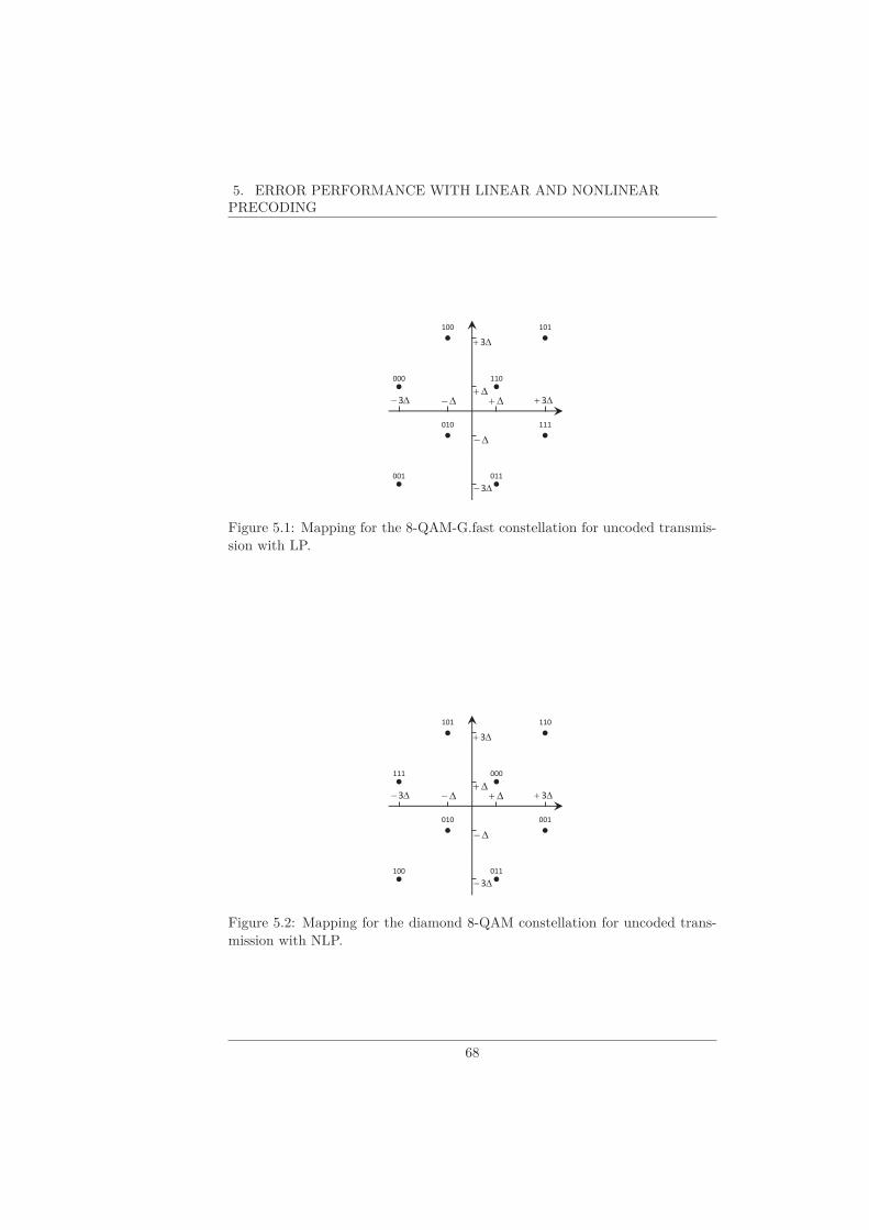
5. ERROR PERFORMANCE WITH LINEAR AND NONLINEARPRECODING
D+
D- D+ D+ 3
D+ 3
D-
D-3
D-3
100 101
000 110
010 111
001 011
Figure 5.1: Mapping for the 8-QAM-G.fast constellation for uncoded transmis-sion with LP.
D+
D- D+ D+ 3
D+ 3
D-
D-3
D-3
101 110
111 000
010 001
100 011
Figure 5.2: Mapping for the diamond 8-QAM constellation for uncoded trans-mission with NLP.
68

5.1. UNCODED TRANSMISSION
D+ 3
D+D- D+ D+ 3
D-
D-3
D-3
01100 01000 11000 11100
01101 01001 11001 11101
01111 01011 11011 11111
01110 01010 11010 11110
00000 00001 10001 10000
10100
10101
10111
10110
00010 00011 10011 10010
00100
00101
00111
00110
D- 5 D+ 5
D+ 5
D- 5
10001
10011
10010
D+ 3
D+D- D+ D+ 3
D-
D-3
D-3
01100 01000 11000 11100
01101 01001 11001 11101
01111 01011 11011 11111
01110 01010 11010 11110
00000
00001
10000 10100
10101
10111
10110 00010
00011
00100
00101
00111
00110
D- 5 D+ 5
D+ 5
D- 5
D-7 D+ 7
ß
Figure 5.3: Transformation of a rectangular 32-QAM constellation into a cross32-QAM constellation.
69

5. ERROR PERFORMANCE WITH LINEAR AND NONLINEARPRECODING
5.1.2 Nonlinear Precoding
5.1.2.1 Detection Algorithm
In the case of nonlinear precoding, as explained in Section 4.4, the scaled androtated observation z(k) is given by (5.2) where a(k)+ l(k)A(k) can be interpretedas a symbol belonging to the periodic extension of the normalized M (k)-QAM
constellation A(k); this extended constellation is denoted A(k)ext. The symbol
decision a(k) is given by
a(k) = arg mina∈A(k)
(
minl∈Z+jZ
∣∣∣z(k) −
√
SNR(k)(
a + lA(k))∣
∣∣
2)
(5.7)
= arg mina∈A(k)
(
minl∈Z+jZ
∣∣∣∣
[
z(k)]
√SNR(k)A(k)
−√
SNR(k)(
a + lA(k))
∣∣∣∣
2)
(5.8)
It follows from (5.8) that[
z(k)]
√SNR(k)A(k)
, which results from a modulo oper-
ation on z(k), is a sufficient statistic for performing the ML decision.
5.1.2.2 Error Performance
The resulting BER related to the detection of the symbol a(k) is given by an
expression similar to (5.4), i.e.,
BER(k) ≈ 1
M (k)
∑
a ∈ A(k), a ∈ A(k)ext,i
|a − a| = d(k)
Nbit(a, a)
log2(M(k))
Q
√(d(k)
)2
2SNR(k)
(5.9)
The difference between (5.4) and (5.9) is in the summation over a: for LP and
NLP, a belongs to the original constellation A(k) and to the extended constella-
tion A(k)ext, respectively; hence, for given constellation sizes and SNRs per tone,
NLP yields the larger BER because A(k) ⊂ A(k)ext. The BER averaged over all
Nt tones is given by (5.5), with BER(k) given by (5.9).
5.1.3 Rule of Thumb
The approximate BER expressions (5.4) for LP and (5.9) for NLP indicate
that the selection of the constellation affects the error performance through
the minimum distance d(k) of the normalized constellation and through the
factor in front of the function Q(.). For large SNR(k), the dependence of d(k)
on the constellation is the more important factor. Hence, when replacing the
normalized constellation A(k) with minimum distance d(k) by the normalized
70

5.1. UNCODED TRANSMISSION
constellation A′(k) with minimum distance d′(k), one should change the SNRfrom SNR(k) to SNR′(k) = (d(k)/d′(k))2SNR(k) in order to maintain essentiallythe same BER at high SNR.
For normalized square-QAM constellations with large M , (4.13) simplifiesto d2 ≈ 6/M . For normalized cross-QAM with large M , (4.15) also yieldsd2 ≈ 6/M , taking into account that 31/32 ≈ 1. Hence, when increasing theconstellation size from M = 2b to M ′ = 2b′
with b′ > b, the error performance ismaintained when increasing the SNR by a factor M ′/M , which corresponds toan increase (expressed in dB) of 10 log(M ′/M ) = 10 log(2) · (b′ − b) ≈ 3(b′ − b).Hence, when increasing the number of bits per QAM symbol by 1 (i.e., whendoubling the number of constellation points), the resulting SNR penalty formaintaining a certain error performance equals about 3 dB.
5.1.4 Numerical Results
In the remainder of this dissertation, we will use the G.fast constellation in thecase of 8-QAM, unless explicitly mentioned otherwise.
Considering the observation models (5.1) and (5.2) for LP and NLP, Fig-ure 5.4 and Figure 5.5 show the corresponding BER for uncoded transmissionfor QAM constellations with b = 1, ...., 12. We observe that the BER approx-imations (5.4) and (5.9), accurately match the simulations results. For largeconstellation sizes, the BER curve for 2b+1-QAM is obtained by shifting theBER curve for 2b-QAM by about 3 dB to the right; this is according to therule of thumb from Section 5.1.3, stating that adding 1 bit to the constellationgives rise to a SNR penalty of about 3 dB. Actually, taking the factor 31/32occuring in the expression (4.15) for the minimum distance for cross-QAM intoaccount, we have for large constellation sizes d2
22n /d222n+1 = 31/16 (2.87 dB))
and d222n+1/d2
22n+2 = 64/31 (3.14 dB); hence, for small BER, the BER curve for22n+1-QAM is not exactly halfway the curves for 22n-QAM and 22n+2-QAM,but slightly closer to the curve for 22n-QAM.
Figure 5.6 shows the BER for NLP with uncoded transmission using thefollowing 8-QAM constellations: 8-QAM-G.fast, 8-QAM-VDSL with A = 8∆
and 8-QAM-VDSL with A = 6∆. 8-QAM-G.fast gives the best performanceat high SNR, as the minimum Euclidean distance between constellation pointsd is larger for G.fast (d2 = 4/5) as compared to VDSL (d2 = 2/3, for bothA = 8∆ and A = 6∆). The better performance of 8-QAM-VDSL with A = 8∆
as compared to A = 6∆ is caused by the larger number of neighbours at minimaldistance when A = 6∆.
Table 5.1 lists the SNR values that are required to achieve BER = 10−7
for the various constellation sizes, for both linear and nonlinear precoding. Weobserve that nonlinear precoding needs a slightly larger SNR, because the ex-
tended constellation A(k)ext,i has more neighbours at minimum Euclidean distance
from the transmitted symbol, when the latter is an outer point of the original
71

5. ERROR PERFORMANCE WITH LINEAR AND NONLINEARPRECODING
0 10 20 30 4010
8
10 6
10 4
10 2
100
SNR!(dB)
BER
b!=!1
b = 2
b = 3
b = 4
b = 5
b = 6
b = 7
b = 8
b = 9
b = 10
b = 11
b = 12
Figure 5.4: BER for LP and uncoded transmission for QAM constellationswith b = 1, . . . , 12; simulations (solid lines with markers) versus approximation(dashed lines).
72

5.1. UNCODED TRANSMISSION
10 20 30 4010
8
10 6
10 4
10 2
100
SNR!(dB)
BER
b!=!1
b!=!2
b!=!3
b!=!4
b!=!5
b!=!6
b!=!7
b!=!8
b!=!9
b!=!10
b!=!11
b!=!12
Figure 5.5: BER for NLP and uncoded transmission for QAM constellationswith b = 1, . . . , 12; simulations (solid lines with markers) versus approximation(dashed lines).
73

5. ERROR PERFORMANCE WITH LINEAR AND NONLINEARPRECODING
6 8 10 12 14 16 18 2010
8
10 6
10 4
10 2
100
SNR!(dB)
BER
b = 3, G.fast
b = 3, VDSL, A = 8∆
b = 3, VDSL, A = 6∆
Figure 5.6: BER for NLP, uncoded transmission and the proposed 8-QAMconstellations; simulations results.
74

5.2. TRELLIS-CODED MODULATION
Table 5.1: Required SNR (in dB) to achieve the target BER of 10−7 for uncodedtransmission with LP and NLP.
b 1 2 3 4 5 6
LP 11.3 14.3 18.3 21.2 24.2 27.4NLP 11.7 14.5 18.5 21.3 24.3 27.4
b 7 8 9 10 11 12
LP 30.3 33.4 36.2 39.3 42.2 45.3NLP 30.3 33.4 36.2 39.4 42.2 45.3
constellation A(k); this effect decreases with increasing constellation size, be-cause of the decreasing relative importance of the outer constellation points ofA(k).
5.2 Trellis-Coded Modulation
In Section 5.2.1, we describe the trellis code used in G.fast and in the VDSLstandard. The detection algorithm and an approximate analytical expressionfor the error performance of TCM is derived in Sections 5.2.2 and 5.2.3, forlinear and nonlinear precoding, respectively. Numerical results are presented inSection 5.2.5. Here we restrict our attention to the case where IN is absent; theeffect of IN will be considered in Section 5.4.
5.2.1 Trellis Code Description
The trellis codes introduced by Ungerboeck typically make use of 2m+1-pointcomplex-valued constellations, such as PSK or QAM constellations, to conveym information bits per constellation; these constellations are referred to as two-dimensional (2-D), because they involve two "real" dimensions. The concept ofTCM has been extended to convey m information bits per 2m+1-point 2Ndim-dimensional constellations (with Ndim > 1), which are obtained as the cartesianproduct of Ndim 2-D constellations [50]. For a given number of information bitsper 2-D symbol, multi-dimensional TCM can be shown to provide a better errorperformance, because of the smaller number of parity bits (i.e. (1/Ndim) paritybits) per 2-D symbol (see Section 5.2.4).
The trellis code, depicted in Figure 5.7, is defined in ITU-T RecommendationG.993.2 [5] and is similar to Wei’s 16-state 4-dimensional trellis code [50]; onlythe symbol mapping is different. At the ℓth trellis section, the trellis encodertransforms an input vector u(ℓ) of z(ℓ) information bits into z(ℓ) + 1 coded bits,i.e., one redundant bit is added. These z(ℓ) + 1 coded bits are split into a set
75
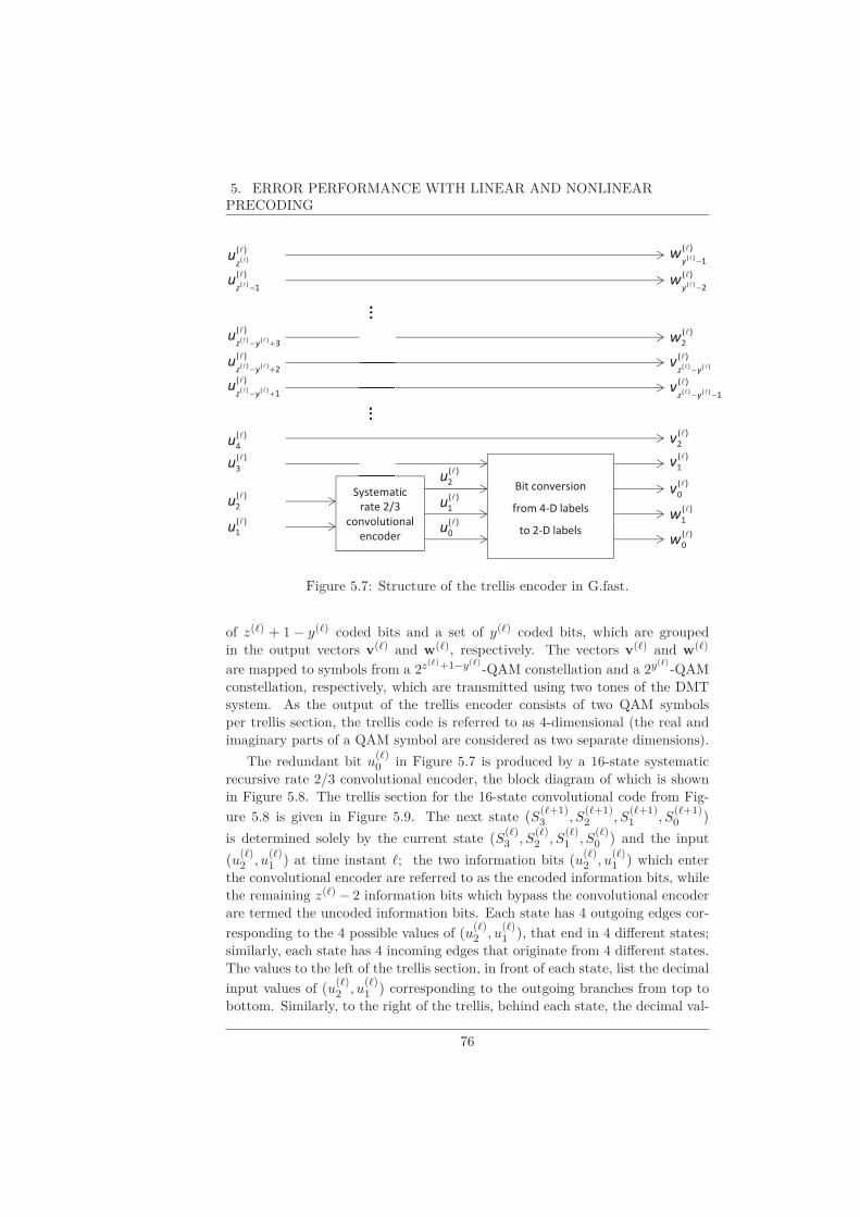
5. ERROR PERFORMANCE WITH LINEAR AND NONLINEARPRECODING
Systematic
rate 2/3
convolutional
encoder
SystematBit conversion
from 4-D labels
to 2-D labels )(
1
lu
)(
2
lu
)(
3
lu
)(
4
lu
)(
1)()(
l
ll+-yz
u
)(
2)()(
l
ll+-yz
u
)(
3)()(
l
ll+-yz
u
)(
1)(
l
l-z
u
)()(
l
lz
u
)(
1
lu
)(
2
lu
)(
0
lu
)(
0
lw
)(
1
lw
)(
0
lv
)(
1
lv
)(
2
lv
)(
1)()(
l
ll--yz
v
)()()(
l
llyz
v-
)(
2
lw
)(
2)(
l
l-y
w
)(
1)(
l
l-y
w
Figure 5.7: Structure of the trellis encoder in G.fast.
of z(ℓ) + 1 − y(ℓ) coded bits and a set of y(ℓ) coded bits, which are groupedin the output vectors v(ℓ) and w(ℓ), respectively. The vectors v(ℓ) and w(ℓ)
are mapped to symbols from a 2z(ℓ)+1−y(ℓ) -QAM constellation and a 2y(ℓ) -QAMconstellation, respectively, which are transmitted using two tones of the DMTsystem. As the output of the trellis encoder consists of two QAM symbolsper trellis section, the trellis code is referred to as 4-dimensional (the real andimaginary parts of a QAM symbol are considered as two separate dimensions).
The redundant bit u(ℓ)0 in Figure 5.7 is produced by a 16-state systematic
recursive rate 2/3 convolutional encoder, the block diagram of which is shownin Figure 5.8. The trellis section for the 16-state convolutional code from Fig-
ure 5.8 is given in Figure 5.9. The next state (S(ℓ+1)3 ,S
(ℓ+1)2 ,S
(ℓ+1)1 ,S
(ℓ+1)0 )
is determined solely by the current state (S(ℓ)3 ,S
(ℓ)2 ,S
(ℓ)1 ,S
(ℓ)0 ) and the input
(u(ℓ)2 ,u
(ℓ)1 ) at time instant ℓ; the two information bits (u
(ℓ)2 ,u
(ℓ)1 ) which enter
the convolutional encoder are referred to as the encoded information bits, whilethe remaining z(ℓ) − 2 information bits which bypass the convolutional encoderare termed the uncoded information bits. Each state has 4 outgoing edges cor-
responding to the 4 possible values of (u(ℓ)2 ,u
(ℓ)1 ), that end in 4 different states;
similarly, each state has 4 incoming edges that originate from 4 different states.The values to the left of the trellis section, in front of each state, list the decimal
input values of (u(ℓ)2 ,u
(ℓ)1 ) corresponding to the outgoing branches from top to
bottom. Similarly, to the right of the trellis, behind each state, the decimal val-
76
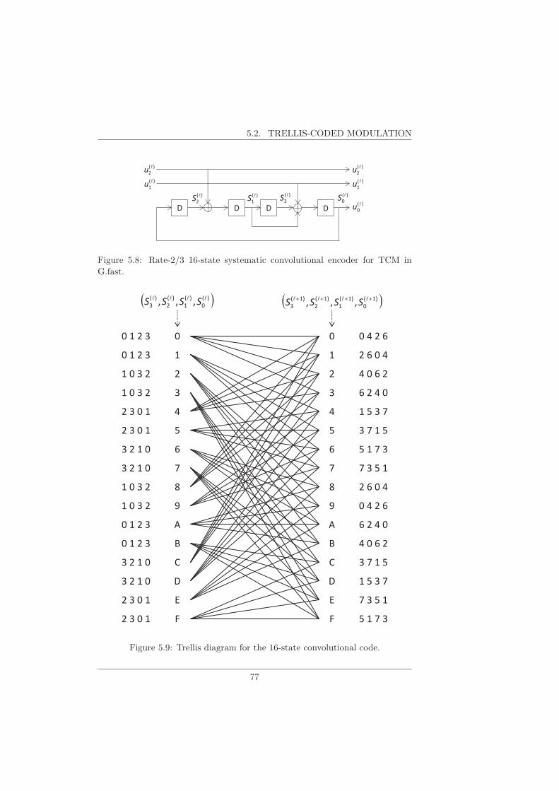
5.2. TRELLIS-CODED MODULATION
)(
0
lS
D D D D
)(
1
lu
)(
2
lu
)(
1
lu
)(
2
lu
)(
0
lu
)(
2
lS
)(
1
lS
)(
3
lS
Figure 5.8: Rate-2/3 16-state systematic convolutional encoder for TCM inG.fast.
0
1
2
3
5
4
7
6
8
D
C
9
E
B
A
F
0
1
2
3
5
4
7
6
8
D
C
9
E
B
A
F
0 1 2 3
0 1 2 3
1 0 3 2
1 0 3 2
2 3 0 1
2 3 0 1
3 2 1 0
3 2 1 0
1 0 3 2
3 2 1 0
3 2 1 0
1 0 3 2
2 3 0 1
0 1 2 3
0 1 2 3
2 3 0 1
0 4 2 6
2 6 0 4
4 0 6 2
6 2 4 0
3 7 1 5
1 5 3 7
7 3 5 1
5 1 7 3
2 6 0 4
1 5 3 7
3 7 1 5
0 4 2 6
7 3 5 1
4 0 6 2
6 2 4 0
5 1 7 3
( ))(
0
)(
1
)(
2
)(
3 ,,,llll
SSSS ( ))1(
0
)1(
1
)1(
2
)1(
3 ,,,++++ llll
SSSS
Figure 5.9: Trellis diagram for the 16-state convolutional code.
77
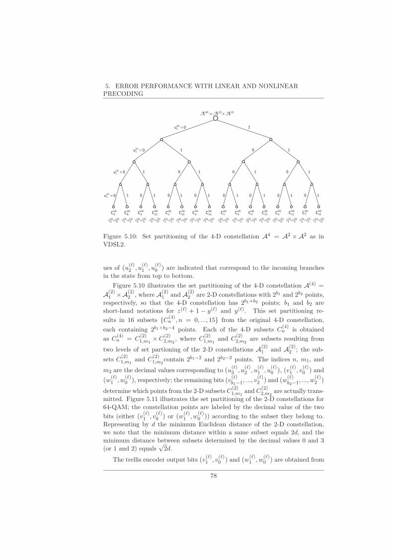
5. ERROR PERFORMANCE WITH LINEAR AND NONLINEARPRECODING
0)3(=
nu
0)2(=
nu
0)1(=
nu
0)0(=
nu
(2)0
C(2)0
C
(4)
0C
´(2)3
C(2)3
C
(4)
8C
´(2)3
C(2)0
C
(4)
4C
´(2)0
C(2)3
C
(4)
12C
´(2)2
C(2)2
C
(4)
2C
´(2)1
C(2)1
C
(4)
10C
´(2)1
C(2)2
C
(4)
6C
´(2)2
C(2)1
C
(4)
14C
´(2)2
C(2)0
C
(4)
1C
´(2)1
C(2)3
C
(4)
9C
´(2)1
C(2)0
C
(4)
5C
´(2)2
C(2)3
C
(4)
13C
´(2)0
C(2)2
C
(4)
3C
´(2)3
C(2)1
C
(4)
11C
´(2)3
C(2)2
C
(4)
7C
´(2)0
C(2)1
C
(4)
15C
´
6
.
7
0 0 0 0 0 0 0
0
0
1
1 1
1 1 1 0
1 1 1 1 1 1 1 1
)2()2()4(AAA ´=
1 0
Figure 5.10: Set partitioning of the 4-D constellation A4 = A2 × A2 as inVDSL2.
ues of (u(ℓ)2 ,u
(ℓ)1 ,u
(ℓ)0 ) are indicated that correspond to the incoming branches
in the state from top to bottom.
Figure 5.10 illustrates the set partitioning of the 4-D constellation A(4) =
A(2)1 × A(2)
2 , where A(2)1 and A(2)
2 are 2-D constellations with 2b1 and 2b2 points,respectively, so that the 4-D constellation has 2b1+b2 points; b1 and b2 areshort-hand notations for z(ℓ) + 1 − y(ℓ) and y(ℓ). This set partitioning re-
sults in 16 subsets {C(4)n ,n = 0, ..., 15} from the original 4-D constellation,
each containing 2b1+b2−4 points. Each of the 4-D subsets C(4)n is obtained
as C(4)n = C
(2)1,m1
× C(2)2,m2
, where C(2)1,m1
and C(2)2,m2
are subsets resulting from
two levels of set partioning of the 2-D constellations A(2)1 and A(2)
2 ; the sub-
sets C(2)1,m1
and C(2)1,m2
contain 2b1−2 and 2b2−2 points. The indices n, m1, and
m2 are the decimal values corresponding to (u(ℓ)3 ,u
(ℓ)2 ,u
(ℓ)1 ,u
(ℓ)0 ), (v
(ℓ)1 , v
(ℓ)0 ) and
(w(ℓ)1 ,w
(ℓ)0 ), respectively; the remaining bits (v
(ℓ)b1−1, ..., v
(ℓ)2 ) and (w
(ℓ)b2−1, ...,w
(ℓ)2 )
determine which points from the 2-D subsets C(2)1,m1
and C(2)2,m2
are actually trans-mitted. Figure 5.11 illustrates the set partitioning of the 2-D constellations for64-QAM; the constellation points are labeled by the decimal value of the two
bits (either (v(ℓ)1 , v
(ℓ)0 ) or (w
(ℓ)1 ,w
(ℓ)0 )) according to the subset they belong to.
Representing by d the minimum Euclidean distance of the 2-D constellation,we note that the minimum distance within a same subset equals 2d, and theminimum distance between subsets determined by the decimal values 0 and 3(or 1 and 2) equals
√2d.
The trellis encoder output bits (v(ℓ)1 , v
(ℓ)0 ) and (w
(ℓ)1 ,w
(ℓ)0 ) are obtained from
78

5.2. TRELLIS-CODED MODULATION
1 3
0 2
1 3
0 2
1
0
1
0
3
2
3
2
1 3 1 3 1 3
0 2 0 2 0 2
1 3 1 3 1 3
1 3 1 3 1 3
1 3 1 3 1 3
0 2 0 2 0 2
0 2 0 2 0 2
0 2 0 2 0 2
Figure 5.11: Mapping of 2-D subsets in 64-QAM.
the bits (u(ℓ)3 ,u
(ℓ)2 ,u
(ℓ)1 ,u
(ℓ)0 ) according to the following modulo-2 additions:
v(ℓ)1 = u
(ℓ)1 ⊕ u
(ℓ)3
v(ℓ)0 = u
(ℓ)3
w(ℓ)1 = u
(ℓ)0 ⊕ u
(ℓ)1 ⊕ u
(ℓ)2 ⊕ u
(ℓ)3
w(ℓ)0 = u
(ℓ)2 ⊕ u
(ℓ)3
The remaining z(ℓ) − 3 trellis encoder output bits are equal to the z(ℓ) − 3 infor-
mation bits that are obtained by removing the information bits (u(ℓ)3 ,u
(ℓ)2 ,u
(ℓ)1 )
from the information bit vector u(ℓ).
From the above description, it follows that the minimum number of infor-
mation bits in a trellis section equals three (i.e., the bits (u(ℓ)3 ,u
(ℓ)2 ,u
(ℓ)1 )), which
corresponds to two 4-QAM symbols, determined by the bits (v(ℓ)1 , v
(ℓ)0 ) and
(w(ℓ)1 ,w
(ℓ)0 ), respectively. When some of the tones convey 2-QAM symbols, two
such symbols are ’paired’ to form a 4-QAM symbol. More specifically, denot-ing the two (normalized) 2-QAM symbols as a2QAM,l = αl(1+ j)/
√2 where
αl ∈ {−1, 1} and l = 1, 2, the corresponding (normalized) 4-QAM symbol ob-tained after pairing is given by a4QAM = (α1 + jα2)/
√2.
The QAM symbols from the TCM codeword are transmitted using the DMTcommunication system. Each subcarrier of the DMT system conveys a QAMsymbol from the TCM codeword. The number of QAM symbols in the TCMcodeword equals the number of tones in the DMT symbol, so that one TCMcodeword corresponds to one DMT symbol.
For the square-QAM and cross-QAM constellations, we use the mappings asproposed in [42]. In Figure 5.2, we show the mapping for 8-QAM-G.fast, where
the last two bits represent either (v(ℓ)1 , v
(ℓ)0 ) or (w
(ℓ)1 ,w
(ℓ)0 ), which determine the
2-D subset to which the constellation point belongs.
79

5. ERROR PERFORMANCE WITH LINEAR AND NONLINEARPRECODING
5.2.2 Linear Precoding
5.2.2.1 Detection Algorithm
We consider the observation model (5.1) in the case of LP, with the user in-dex removed for notational convenience. Applying ML sequence detection,
the detected symbol sequence a =(
a(1), a(2), ..., a(Nt))
is obtained as a =
argmina∈C
DLP(a), where
DLP(a) =Nt∑
k=1
∣∣∣z(k) −
√
SNR(k)a(k)∣∣∣
2
(5.10)
a =(
a(1), a(2), ..., a(Nt))
and the minimization is over the set C of valid coded
symbol sequences. This minimization is executed efficiently by applying the
Viterbi algorithm to the trellis that describes the operation of the trellis en-
coder. As the state transition at the ℓth trellis section is determined only
by the current state (S(ℓ)3 ,S
(ℓ)2 ,S
(ℓ)1 ,S
(ℓ)0 ) and the information bits (u
(ℓ)2 ,u
(ℓ)1 ),
it follows that for a given current state the different information bit vectors
u(ℓ) which have the same (u(ℓ)2 ,u
(ℓ)1 ) give rise to the same state transition.
Hence, each state transition in the trellis of the rate 2/3 convolutional code
(see Figure 5.9) turns into 2z(ℓ)−2 parallel transitions (corresponding to theuncoded information bits) in the trellis of the trellis code. Each of these par-
allel transitions corresponds to a different 4-D symbol; these 4-D symbols have
the bits (u(ℓ)2 ,u
(ℓ)1 ,u
(ℓ)0 ) in common. The branch metric to be used in the
Viterbi algorithm for a given state transition at the ℓth trellis section is given
by mina(2ℓ),a(2ℓ+1)
(
D(2ℓ)LP (a(2ℓ)) + D
(2ℓ+1)LP (a(2ℓ+1))
)
, where
D(k)LP (a
(k)) =∣∣∣z(k) −
√
SNR(k)a(k)∣∣∣
2
(5.11)
and the minimization is over the 4-D symbols (a(2ℓ), a(2ℓ+1)) associated withthe parallel transitions corresponding to the considered state transition. In the
case where a 4-QAM symbol a(k) is the result of the pairing of two 2-QAM
symbols a(k1) and a(k2) with associated observations z(k1) and z(k2) , we have
D(k)LP (a
(k)) =∣∣∣z(k1) −
√
SNR(k1)a(k1)∣∣∣
2
+∣∣∣z(k2) −
√
SNR(k2)a(k2)∣∣∣
2
where a(k1) = (1+ j)ℜ(a(k)) and a(k2) = (1+ j)ℑ(a(k)).
5.2.2.2 Error Performance
The pairwise error probability PEP(a|a) = Pr[DLP(a) < DLP(a)|a] is an upperbound on the probability that the ML decision equals a, when the transmitted
80

5.2. TRELLIS-CODED MODULATION
symbol vector equals a. It is easily verified that
PEP(a|a) = Q
√√√√1
2
Nt∑
k=1
|∆a(k)|2SNR(k)
(5.12)
where ∆a(k) = a(k) − a(k). The resulting BER is upper bounded as
BER ≤∑
a,a Ninfo(a, a)PEP(a|a)Pr[a]∑Nt
k=1
(log2(M
(k)) − 1/2) (5.13)
where the summation in the numerator is over all allowed coded symbol se-quences a ∈ C and a ∈ C, Ninfo(a, a) denotes the number of information bits that
are different between the coded sequences a and a, Pr[a] = 2Nt/2∏Nt
k=1
(
M (k))−1
is the a priori probability that the transmitted coded sequence equals a, and thedenominator of (5.13) equals the number of information bits within the DMTsymbol.
Now we restrict our attention to the case where the constellations and theSNRs are the same for all Nt tones, i.e., M (k) = M and SNR(k) = SNR for allk, so that (5.12) and (5.13) reduce to
PEP(a|a) = Q
(√
SNR
2|∆a|2
)
BER ≤∑
a,a Ninfo(a, a)PEP(a|a)Pr[a](log2(M ) − 1/2)Nt
(5.14)
and Pr[a] =(√
2/M)Nt . For a given transmitted coded symbol sequence a, the
upper bound on BER is dominated by the coded symbol sequences a with a Ó= a,for which the Euclidean distance |∆a|2 is the smallest. Let us consider the casewhere a differs from a in the ℓth trellis section only: (a(2ℓ), a(2ℓ+1)) representsa 4-D symbol on a branch connecting the same states as the branch that carriesthe 4-D symbol (a(2ℓ), a(2ℓ+1)), i.e., these two branches correspond to parallel
transitions. Hence, these two 4-D symbols have the bits (u(ℓ)2 ,u
(ℓ)1 ,u
(ℓ)0 ) in
common, so they differ only in the uncoded information bits. The followingcases can be distinguished.
1. The two 4-D symbols have also the bit u(ℓ)3 in common. The 2-D symbols
a(2ℓ) and a(2ℓ) belong to a same subset C(2)1,m1
, and a(2ℓ+1) and a(2ℓ+1)
belong to a same subset C(2)2,m2
; a point from either subset has (at most) 4nearest neighbours at distance 2d (with d representing the minimum Eu-clidean distance of the M -QAM constellation). Hence, the correspondingminimum |∆a|2 equals 4d2, which is obtained when either a(2ℓ) = a(2ℓ),and a(2ℓ+1) is a nearest neighbour of a(2ℓ+1) (at most 4 possibilities for
81

5. ERROR PERFORMANCE WITH LINEAR AND NONLINEARPRECODING
a(2ℓ+1) ), or a(2ℓ+1) = a(2ℓ+1), and a(2ℓ) is a nearest neighbor of a(2ℓ) (atmost 4 possibilities for a(2ℓ) ). This corresponds to a total of (at most) 8possibilities to obtain |∆a|2 = 4d2; the number of possibilities is less than8 when the transmitted 2-D constellation points are near the edges of theconstellation.
2. The bit u(ℓ)3 is different for the two 4-D symbols. The 2-D symbols a(2ℓ)
and a(2ℓ) belong to different subsets C(2)1,m1
, with (at most) 4 neighbours
at minimum interset distance√2d; the same holds for a(2ℓ+1) and a(2ℓ+1).
Hence, the corresponding minimum |∆a|2 equals 4d2, which is obtainedwhen a(2ℓ) is at distance
√2d from a(2ℓ) (at most 4 possibilities), and
a(2ℓ+1) is at distance√2d from a(2ℓ+1) (at most 4 possibilities). This
corresponds to a total of (at most) 16 possibilities to obtain |∆a|2 =4d2; the number of possibilities is less than 16 when the transmitted 2-Dconstellation points are near the edges of the constellation.
When a differs from a in more than one trellis section, it can be verified fromthe trellis that |∆a|2 ≥ 5d2. Hence, at high SNR, the upper bound (5.14) onBER is dominated by the coded sequences a that differ from a in one trellissection only, yielding |∆a|2 = 4d2. Approximating BER by keeping in (5.14)only the terms with |∆a|2 = 4d2, we obtain
BER ≈∑
a, a
|∆a| = 2d
Ninfo(a, a)
(log2(M ) − 1/2)NtPr[a]Q
(√2d2SNR
)
(5.15)
A simple estimate of the factor in front of Q(√
2d2SNR)
in (5.15) is obtained
by assuming that for each a there are 12Nt sequences a for which |∆a|2 = 4d2
(i.e., Nt/2 trellis sections and 24 parallel transitions at minimum distance fromthe correct transition), and that half the number of information bits in theconsidered trellis section is wrong (i.e., (log2(M ) − 1/2) erroneous informationbits); this yields
BER ≈ 12Q(√
2d2SNR)
(5.16)
Note that the factor of 12 involves an overestimation of the number of codedsequences a at minimum distance from a, especially for small constellations.
5.2.3 Nonlinear Precoding
5.2.3.1 Detection Algorithm
In the case of nonlinear precoding, the observation model (5.2) holds, withthe user index removed for notational convenience. The symbol sequence a =(
a(1), a(2), ..., a(Nt))
resulting from ML sequence detection is obtained as a =
82
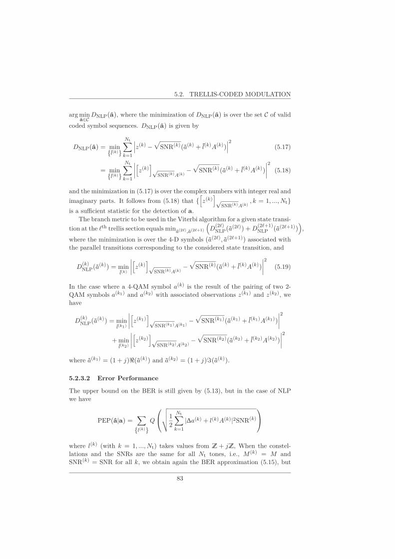
5.2. TRELLIS-CODED MODULATION
argmina∈C
DNLP(a), where the minimization of DNLP(a) is over the set C of valid
coded symbol sequences. DNLP(a) is given by
DNLP(a) = min{l(k)}
Nt∑
k=1
∣∣∣z(k) −
√
SNR(k)(a(k) + l(k)A(k))∣∣∣
2
(5.17)
= min{l(k)}
Nt∑
k=1
∣∣∣∣
[
z(k)]
√SNR(k)A(k)
−√
SNR(k)(a(k) + l(k)A(k))
∣∣∣∣
2
(5.18)
and the minimization in (5.17) is over the complex numbers with integer real and
imaginary parts. It follows from (5.18) that {[
z(k)]
√SNR(k)A(k)
, k = 1, ...,Nt}is a sufficient statistic for the detection of a.
The branch metric to be used in the Viterbi algorithm for a given state transi-
tion at the ℓth trellis section equalsmina(2ℓ),a(2ℓ+1)
(
D(2ℓ)NLP(a
(2ℓ)) + D(2ℓ+1)NLP (a(2ℓ+1))
)
,
where the minimization is over the 4-D symbols (a(2ℓ), a(2ℓ+1)) associated withthe parallel transitions corresponding to the considered state transition, and
D(k)NLP(a
(k)) = minl(k)
∣∣∣∣
[
z(k)]
√SNR(k)A(k)
−√
SNR(k)(a(k) + l(k)A(k))
∣∣∣∣
2
(5.19)
In the case where a 4-QAM symbol a(k) is the result of the pairing of two 2-
QAM symbols a(k1) and a(k2) with associated observations z(k1) and z(k2), we
have
D(k)NLP(a
(k)) = minl(k1)
∣∣∣∣
[
z(k1)]
√SNR(k1)A(k1)
−√
SNR(k1)(a(k1) + l(k1)A(k1))
∣∣∣∣
2
+minl(k2)
∣∣∣∣
[
z(k2)]
√SNR(k2)A(k2)
−√
SNR(k2)(a(k2) + l(k2)A(k2))
∣∣∣∣
2
where a(k1) = (1+ j)ℜ(a(k)) and a(k2) = (1+ j)ℑ(a(k)).
5.2.3.2 Error Performance
The upper bound on the BER is still given by (5.13), but in the case of NLP
we have
PEP(a|a) =∑
{l(k)}Q
√√√√1
2
Nt∑
k=1
|∆a(k) + l(k)A(k)|2SNR(k)
where l(k) (with k = 1, ...,Nt) takes values from Z + jZ, When the constel-
lations and the SNRs are the same for all Nt tones, i.e., M (k) = M and
SNR(k) = SNR for all k, we obtain again the BER approximation (5.15), but
83

5. ERROR PERFORMANCE WITH LINEAR AND NONLINEARPRECODING
now a belongs to the set Cext containing not only all allowed coded symbol se-quences from C but also the sequences for which the modulo reduction (the kth
component a(k) is reduced modulo A(k), k = 1, ...,Nt) belongs to C. As thereare more sequences in this augmented set Cext at minimum distance 2d fromthe transmitted sequence than in the set C, the resulting BER for NLP is larger
than for LP, because of a larger coefficient in front of Q(√
2d2SNR)
.
5.2.4 Rule of Thumb
Making a similar reasoning as in Section 5.1.3, it follows from the approximate
BER expression (5.15) that doubling the number of constellation points from
2b to 2b+1 requires the SNR to be increased by about 3 dB in order to maintain
the same TCM error performance (assuming SNR and 2b to be large).
Now let us compare the error performances of TCM and uncoded trans-
mission. Comparing the arguments of the function Q(.) in (5.15) and (5.4) or(5.9), we observe that for a given constellation, uncoded transmission requires
a 6 dB higher SNR, compared to TCM, in order to achieve the same error per-
formance as TCM (assuming large SNR). However, when uncoded transmission
and TCM use the same constellation, they operate at different information bi-
trates. Taking into account that TCM introduces 1 parity bit per Ndim QAM
symbols (in G.fast, we have Ndim = 2, which is referred to as 4D TCM) a
2b-QAM constellation carries b − (1/Ndim) information bits. Hence, for a faircomparison, we should compare TCM with a 2b-QAM constellation to uncoded
2b−(1/Ndim)-QAM. It follows from Section 5.1.3 that, compared to uncoded 2b-
QAM, uncoded 2b−(1/Ndim)-QAM requires about 3/Ndim dB less SNR in order
to achieve the same error performance. Hence, comparing TCM using 2b-QAM
to uncoded 2b−(1/Ndim)-QAM (yielding the same information bitrate), the for-
mer has a coding gain of 6− (3/Ndim) dB; for Ndim equal to 1, 2 and 4, the
corresponding coding gains are 3 dB, 4.5 dB and 5.25 dB, respectively, which il-
lustrates the performance advantage of using multi-dimensional TCM compared
to the 2D TCM (i.e., Ndim = 1) originally proposed by Ungerboeck.
When comparing uncoded 2b-QAM to uncoded 2b−(1/Ndim)-QAM, we ap-
plied the rule of thumb from Section 5.1.3 to uncoded QAM in spite of a non-
integer number of information bits (i.e., b − (1/Ndim) bits) per QAM symbol.
In a practical setting, the corresponding information bitrate could be achieved
by time-multiplexing uncoded 2b-QAM and uncoded 2b−1-QAM, with fractionsof the time equal to 1− (1/Ndim) and 1/Ndim, respectively. Denoting by E the
constellation energy needed for uncoded 2b-QAM to achieve a certain error per-
formance, an average constellation energy for the time-multiplexed signal equal
to (1− (1/Ndim))E + (1/Ndim)(E/2) = (1− (1/(2Ndim)))E yields essentiallythe same error performance, but at an SNR which is −10 log(1− (1/(2Ndim)))dB less than for uncoded 2b-QAM; for Ndim equal to 1, 2 and 4, the correspond-
ing advantage of the time-multiplex compared to uncoded 2b-QAM amounts to
84

5.2. TRELLIS-CODED MODULATION
0 10 20 30 4010
8
10 6
10 4
10 2
100
SNR!(dB)
BER
b!=!1
b!=!2
b!=!3
b!=!4
b!=!5
b!=!6
b!=!7
b!=!8
b!=!9!
b!=!10
b!=!11
b!=!12
Figure 5.12: BER performance of TCM with LP for constant constellation size,simulations (solid lines with markers) versus approximation (dashed lines).
3 dB, 1.25 dB and 0.58 dB. The rule from Section 5.1.3 indicates an advantageof about 3/Ndim dB for uncoded 2b−(1/Ndim) compared to uncoded 2b-QAM,which for Ndim equal to 1, 2 and 4 corresponds to 3 dB, 1.5 dB and 0.75 dB;note that these results are at most only a few tenths of a dB different from theresults for the time-multiplex.
5.2.5 Numerical Results
In Figure 5.12, the BER performance is shown for TCM with LP under theassumption that on each tone a 2b-QAM constellation is used, and all toneshave the same SNR. The considered constellations range from 2-bit QAM to 12-bit QAM. For each constellation size, both the BER resulting from simulationsand the approximated BER is given. For b ≥ 5 we use the approximation
12Q(√
2d2SNR)
, which turns out to be quite accurate for small BER. For
b < 5 this approximation is less accurate (the number of codewords at minimumdistance is severely overestimated), so we use (5.15) instead, which provides anaccurate approximation at low BER.
Figure 5.13 shows the BER performance for TCM with NLP; again both theBER resulting from simulations and the approximated BER is given. Due to the
85

5. ERROR PERFORMANCE WITH LINEAR AND NONLINEARPRECODING
0 10 20 30 4010
8
10 6
10 4
10 2
100
SNR!(dB)
BER
b!=!1
b!=!2
b!=!3
b!=!4
b!=!5
b!=!6
b!=!7
b!=!8
b!=!9
b!=!10
b!=!11
b!=!12
Figure 5.13: BER performance of TCM with NLP for constant constellationsize, simulations (solid lines with markers) versus approximation (dashed lines).
augmented set of allowed coded symbol sequences at minimal distance for NLP,
the approximation 12Q(√
2d2SNR)
turns out to be accurate at low BER for
smaller constellations (b ≥ 3) than was the case for LP. For b = 1 and b = 2, weuse (5.15) instead. For these constellations, a trellis section represents only the
4 bits (u(ℓ)3 ,u
(ℓ)2 ,u
(ℓ)1 ,u
(ℓ)0 ). The only possible parallel transition would result in
an error in bit u(ℓ)3 , corresponding to erroneous symbols on both tones in the
trellis section. The number of codewords at minimum distance is 256 for b = 1
and 16 for b = 2, and all 3 transmitted information bits in the trellis section are
in error. Based on these observations, (5.15) yields BER = 256Q(√
2d2SNR)
and BER = 16Q(√
2d2SNR)
for b = 1 and b = 2 respectively.
To verify the assumption that dominant error events involve only the un-coded bits corresponding to parallel transitions, we performed some additionalsimulations for LP with 16-QAM and Nt = 2048. Figure 5.14 shows the ratioηCW of the number of codewords with decoding errors in the uncoded infor-mation bits only, to the total number of erroneously decoded codewords. Weobserve that ηCW increases with increasing SNR, and reaches the value of about90% for SNR ≈ 16 dB (where BER ≈ 10−7). Figure 5.15 shows the ratio ηinfo of
86

5.2. TRELLIS-CODED MODULATION
10 11 12 13 14 15 16 170
0.1
0.2
0.3
0.4
0.5
0.6
0.7
0.8
0.9
1
SNR (dB)
ηC
W
Figure 5.14: ηCW for TCM and constant constellation size (b = 4).
the number of erroneous uncoded information bits to the total number of erro-neous information bits. This ratio increases with increasing SNR, and reaches avalue of about 85% for SNR ≈ 16 dB. These results illustrate that at large SNRthe errors involving coded information bits can be safely ignored compared tothe errors involving only uncoded information bits.
It can be verified from the trellis diagram that paths which leave the orig-inal path reemerge with the original transmitted path after at least 3 trellissections and have a minimal squared distance of 5d2 to the original transmit-ted sequence, while the parallel transitions have a minimum squared distanceof 4d2. We validate this observation by means of computer simulations. ForLP with normalized 16-QAM (d2 = 2/5) and Nt = 2048, we have obtained
by means of simulation the squared distances∑Nt
k=1 |∆a(k)i |2 for the codewords
containing errors in the encoded information bits. Figure 5.16 shows that theaverage squared distance for these erroneous codewords approaches 5d2 = 2 forlarge SNR values, which is in agreement with the theoretical analysis.
Again by means of simulations, we have investigated the BER performanceof the trellis code, operating on (5.1) for LP and on (5.2) for NLP, assumingthat the constellation size and the SNR are the same for all tones. Table 5.2shows SNRLP(b) and SNRNLP(b) that are required to achieve BER = 10−7 forLP and NLP, respectively, assuming a constellation size M = 2b. We observethat SNRLP(b) ≤ SNRNLP(b), indicating that LP yields the better decoderperformance; SNRLP(b) and SNRNLP(b) are essentially the same for large con-
87

5. ERROR PERFORMANCE WITH LINEAR AND NONLINEARPRECODING
10 11 12 13 14 15 16 170
0.1
0.2
0.3
0.4
0.5
0.6
0.7
0.8
0.9
1
SNR (dB)
ηin
fo
Figure 5.15: ηinfo of TCM for constant constellation size (b = 4).
14 14.5 15 15.5 16 16.52
2.05
2.1
2.15
2.2
2.25
2.3
2.35
2.4
2.45
2.5
SNR (dB)
∑N
t
k=1|∆
a(k)
i|2
Figure 5.16: Average squared distance of the nonparallel error events, for thenormalized 16-QAM constellation.
88
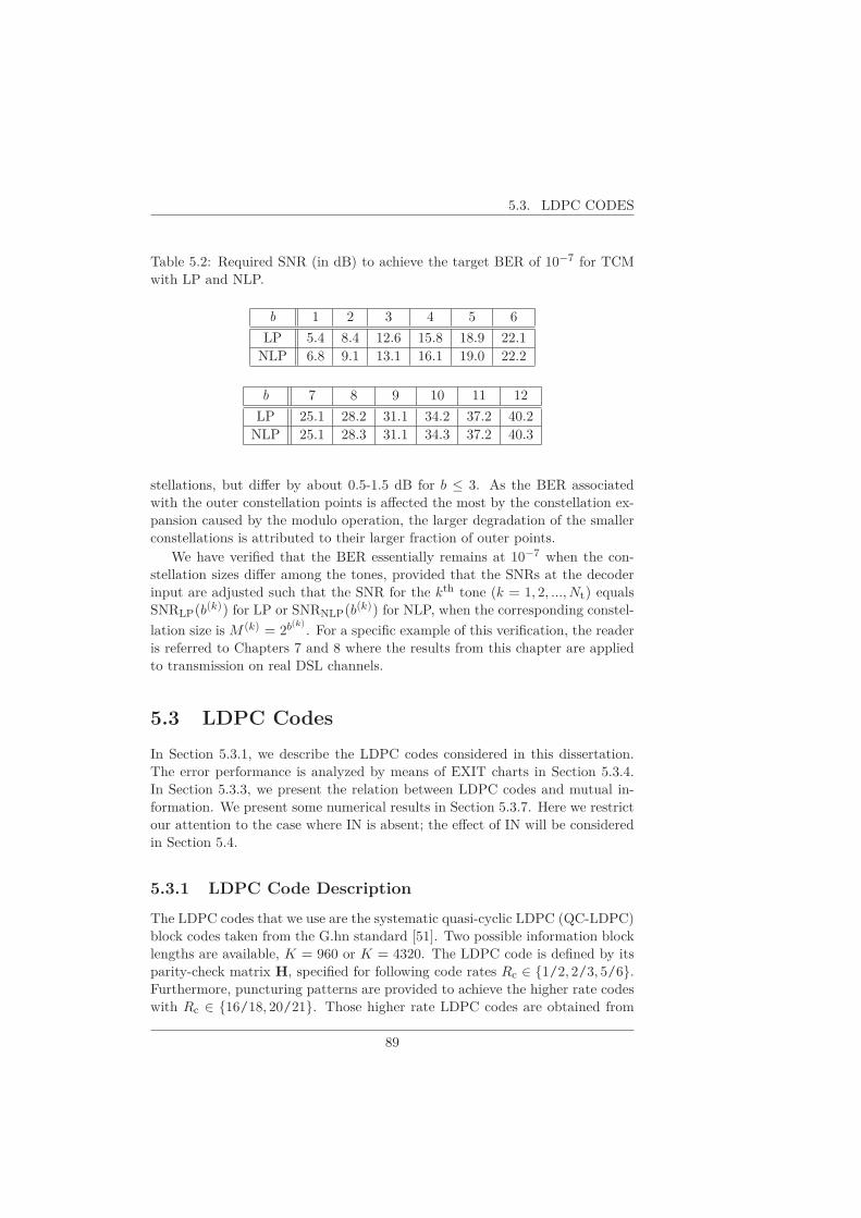
5.3. LDPC CODES
Table 5.2: Required SNR (in dB) to achieve the target BER of 10−7 for TCMwith LP and NLP.
b 1 2 3 4 5 6
LP 5.4 8.4 12.6 15.8 18.9 22.1NLP 6.8 9.1 13.1 16.1 19.0 22.2
b 7 8 9 10 11 12
LP 25.1 28.2 31.1 34.2 37.2 40.2NLP 25.1 28.3 31.1 34.3 37.2 40.3
stellations, but differ by about 0.5-1.5 dB for b ≤ 3. As the BER associatedwith the outer constellation points is affected the most by the constellation ex-pansion caused by the modulo operation, the larger degradation of the smallerconstellations is attributed to their larger fraction of outer points.
We have verified that the BER essentially remains at 10−7 when the con-stellation sizes differ among the tones, provided that the SNRs at the decoderinput are adjusted such that the SNR for the kth tone (k = 1, 2, ...,Nt) equalsSNRLP(b
(k)) for LP or SNRNLP(b(k)) for NLP, when the corresponding constel-
lation size is M (k) = 2b(k) . For a specific example of this verification, the readeris referred to Chapters 7 and 8 where the results from this chapter are appliedto transmission on real DSL channels.
5.3 LDPC Codes
In Section 5.3.1, we describe the LDPC codes considered in this dissertation.The error performance is analyzed by means of EXIT charts in Section 5.3.4.In Section 5.3.3, we present the relation between LDPC codes and mutual in-formation. We present some numerical results in Section 5.3.7. Here we restrictour attention to the case where IN is absent; the effect of IN will be consideredin Section 5.4.
5.3.1 LDPC Code Description
The LDPC codes that we use are the systematic quasi-cyclic LDPC (QC-LDPC)block codes taken from the G.hn standard [51]. Two possible information blocklengths are available, K = 960 or K = 4320. The LDPC code is defined by itsparity-check matrix H, specified for following code rates Rc ∈ {1/2, 2/3, 5/6}.Furthermore, puncturing patterns are provided to achieve the higher rate codeswith Rc ∈ {16/18, 20/21}. Those higher rate LDPC codes are obtained from
89

5. ERROR PERFORMANCE WITH LINEAR AND NONLINEARPRECODING
the ’mother’ code with rate Rc = 5/6 by discarding both some information andparity bits. The codeword length is then given by N = K/Rc.
The check matrix of the QC-LDPC code consists of an array of N−Kh × N
h
circulant h × h sub-matrices Bi,j :
H =
B1,1 B1,2 · · · B1,N
h
B2,1 B2,2 · · · B2,N
h
.... . .
...B N−K
h,1
Bi,j · · · B N−Kh
,Nh
(5.20)
The submatrix Bi,j is equal to either a cyclic column shift of the identity matrixor a zero matrix.
As illustration we present the compact form of the check matrix Hc (thesubscript c refers to "compact") corresponding Rc = 5/6 and K = 960:
Hc =
−1 13 32 47 41 24 −1 25 22 40 1 31
25 46 15 43 45 29 39 47 23 38 39 12
35 45 45 38 14 16 6 11 −1 18 7 41
9 32 6 22 26 31 9 8 22 32 40 4
8 15 20 15 42 30 13 3 −1 0 −1 −1−1 21 −1 38 33 0 0 −1 39 0 0 −135 17 32 45 41 −1 18 17 0 −1 0 0
18 40 36 −1 −1 23 31 41 39 20 −1 0
(5.21)
where -1 stands for a zero h × h sub-matrix and each non-negative integer standsfor a cyclic column shift of the identity matrix, with the number of right columnshifts given by the integer.
Next, the bits in the LDPC codeword are randomly interleaved, and finallythe interleaved codeword is mapped to constellation symbols.
5.3.1.1 Encoding Operation
The systematic codeword c = (cN , . . . , c1) = (uK , . . . ,u1, pN−K , . . . , p1) con-sists of an information part and a parity bit part. For this type of LDPC codes,the parity part can easily be generated without determining the systematic gen-erator matrix G from H such that GHT = 0, normally used for encoding. Thecodeword c = (u|p) satisfies the parity check equations, i.e. cHT = 0:
(u|p) · HT = 0 (5.22)
(u|p) ·(
HT1
HT2
)
= 0 (5.23)
u · HT1 + p · HT
2 = 0 (5.24)
90

5.3. LDPC CODES
where the check matrix HT is decomposed in 2 sub-matrices HT1 and HT
2 re-spectively corresponding to the first K and last N − K rows of HT.
Due to the low number of 1’s per row in HT2 , the system can be solved with
low complexity to find the parity bits (pN−K , . . . , p1).
5.3.1.2 Puncturing
For the sake of illustration, we give here the two puncturing patterns necessaryto obtain the high rate codes with Rc = 16/18 and Rc = 20/21, from theLDPC code defined by the check matrix in (5.21) for K = 960:
pp1080 = [11 . . . 1︸ ︷︷ ︸
720
00 . . . 0︸ ︷︷ ︸
36
11 . . . 1︸ ︷︷ ︸
360
00 . . . 0︸ ︷︷ ︸
36
] (5.25)
pp1008 = [11 . . . 1︸ ︷︷ ︸
720
00 . . . 0︸ ︷︷ ︸
48
11 . . . 1︸ ︷︷ ︸
240
00 . . . 0︸ ︷︷ ︸
96
11 . . . 1︸ ︷︷ ︸
48
] (5.26)
where the puncturing pattern serves as a mask and the jth bit is omitted fromc if ppN ,j = 0.
5.3.2 LDPC Decoding
In the absence of IN, the LDPC decoding is executed according to the SPA usingthe exact computation of the LLRs, as explained in Section 2.3.1.1. In the caseof a punctured LDPC code, the decoder executes the SPA on the Tanner graphof the mother code, with the LLRs of the punctured bits set to zero.
Below we outline the soft demapping (i.e., the computation of the LLRsLch→n) in the cases of linear and nonlinear precoding.
5.3.2.1 Linear Precoder
In the case of LP , the exact LLR (2.2) of the nth coded bit cn, which is containedin the observation z(k) from (5.1), is computed as
Lch→n = ln
∑
a(k)∈A(k)cn=0
exp
(
−∣∣∣z(k) −
√
SNR(k)a(k)∣∣∣
2)
∑
a(k)∈A(k)cn=1
exp
(
−∣∣∣z(k) −
√
SNR(k)a(k)∣∣∣
2) (5.27)
where A(k)cn=0
and A(k)cn=1
represent the subset of the symbol constellation A(k)
corresponding to cn = 0 and cn = 1, respectively.We will consider 2b-QAM constellations (with b = 1, 2, . . . , 12) with the same
mapping as for uncoded transmission (i.e., Gray mapping for b = 1 and evenb; close-to-Gray mapping for odd b with b ≥ 3), which minimizes the averagenumber of bit differences between constellation points at minimum distance.
91

5. ERROR PERFORMANCE WITH LINEAR AND NONLINEARPRECODING
5.3.2.2 Nonlinear Precoder
In the case of NLP, the LLR (2.2) of the nth coded bit un, which is containedin the observation z(k) from (5.2), is computed as
Lch→n = ln
∑
a(k)∈A(k)ext,cn=0
exp
(
−∣∣∣z(k) −
√
SNR(k)a(k)∣∣∣
2)
∑
a(k)∈A(k)ext,cn=1
exp
(
−∣∣∣z(k) −
√
SNR(k)a(k)∣∣∣
2) (5.28)
where A(k)ext,cn=0
and A(k)ext,cn=1
represent the subset of the extended symbol
constellation A(k)ext corresponding to cn = 0 and cn = 1, respectively.
The system with NLP uses the same constellations and mappings as forLP, with one exception for 8-QAM. For 8-QAM-G.fast, we use the mappingfrom Figure 5.2, instead of the mapping from Figure 5.1 as used with LP. Thischoice is justified by the fact that the extended symbol constellation with themapping from Figure 5.2 yields a lower average bit difference between points atminimum distance, as compared to the extended signal constellation with themapping from Figure 5.1.
5.3.3 Mutual Information of LLRs
Here we consider the average mutual information Iavg between a coded bit cn
and its corresponding LLR Lch→n. We will point out that this mutual informa-tion plays an important role in the analysis of the LDPC decoding performance.
Assume that the coded bit cn is the jth bit of the symbol a(k) which belongs
to a 2b(k) -QAM constellation A(k). For notational convenience, we represent cn
and the corresponding LLR Lch→n by c(k)j and L
(k)j , respectively. The mutual
information I(c(k)j ;L
(k)j ) between c
(k)j and L
(k)j depends on the bit index j and
the constellation A(k), and is denoted Ij,A(k) :
Ij,A(k) = I(c
(k)j ;L
(k)j ) (5.29)
=∑
c(k)j
∈{0,1}
∫
L(k)j
pc,L(c(k)j ,L
(k)j ) log2
pc,L(c
(k)j ,L
(k)j )
pc(c(k)j ) · pL(L
(k)j )
dL(k)j (5.30)
Averaging Ij,A(k) over the b(k) bits of the considered constellation A(k) yields
the average mutual information IA(k) :
IA(k) =1
b(k)
b(k)∑
j=1
Ij,A(k)
92

5.3. LDPC CODES
Finally, taking into account that b(k) coded bits each yield on average a mutualinformation equal to IA(k) , the average mutual information Iavg over all codedbits is obtained as
Iavg =
∑Ntk=1 b(k)IA(k)∑Nt
k=1 b(k)
When Lch→n is computed according to the exact expressions (5.27) for LP or(5.28) for NLP, Lch→n is a sufficient statistic, implying that Lch→n and z(k)
contain the same information about the coded bit cn. In this case, Ij,A(k) can
be computed as Ij,A(k) = I(c
(k)j ; z(k)), which simplifies the computation.
Assuming that all tones use the same constellation and have the same SNR,
Figures 5.17 and 5.18 show Iavg versus SNR for 2b-QAM (b = 1, . . . , 12) and
respectively LP and NLP; the LLRs are computed according to (5.27) for LP
and (5.28) for NLP. Clearly, there is a degradation of Iavg when NLP is used,
especially for Iavg close to 0. This is due to the periodic extensions of the original
QAM constellation that need to be considered during computation of the LLRs.
�10 0 10 20 30 400
0.1
0.2
0.3
0.4
0.5
0.6
0.7
0.8
0.9
1
SNR (dB)
I avg
b = 1
b = 2
b = 3
b = 4
b = 5
b = 6
b = 7
b = 8
b = 9
b = 10
b = 11
b = 12
Figure 5.17: Average mutual information per bit Iavg for 2b-QAM (b =1, . . . , 12), LP.
5.3.4 EXIT Chart Analysis.
The decoding performance of the LDPC codes can be analyzed by examiningtheir EXIT charts (introduced in Section 2.3.2). To approach very low BER,
93

5. ERROR PERFORMANCE WITH LINEAR AND NONLINEARPRECODING
�10 0 10 20 30 40
0.1
0.2
0.3
0.4
0.5
0.6
0.7
0.8
0.9
1
SNR (dB)
I avg
b = 1
b = 2
b = 3
b = 4
b = 5
b = 6
b = 7
b = 8
b = 9
b = 10
b = 11
b = 12
Figure 5.18: Average mutual information per bit Iavg for 2b-QAM (b =1, . . . , 12), NLP.
the EXIT curves related to the variable nodes and the check nodes must bematched: the former curve must be located above the latter curve, so thattheir only crossing point is (1,1). If this is the case, we say that ’the tunnelis open’, which implies that a mutual information increase can be realized bytransferring messages between the variable nodes and the check nodes, with theobjective to eventually obtain a mutual information equal to 1. The closer thecurves fit together, the smaller the increase in mutual information per iterationand the larger the number of decoding iterations that are needed to reach theconvergence point (1,1).
In the following we consider the EXIT charts of the different LDPC codesconsidered in this dissertation. The mutual information IE,V
∣∣IA,V =0
at the
starting point of the variable node EXIT curve equals the average mutual infor-mation Iavg computed in Section 5.3.3. We assume that all tones use a BPSKconstellation and have the same SNR, and that LP is used; hence, the curve forb = 1 in Fig. 5.17 shows the relation between Iavg and SNR.
For the LDPC code of rate 1/2, Figures 5.19 and 5.20 give the variable nodeEXIT curves (for SNR equal to 1 dB) and the check node EXIT curves, respec-tively. The considered LDPC codes are irregular, meaning that multiple variablenode degrees and multiple check node degrees occur: the rate 1/2 LDPC codehas variable node degrees dv ∈ {2, 3, 6} and check node degrees dc ∈ {5, 6, 7}.The variable node EXIT curve is the average, over all occurring degrees dv, of
94

5.3. LDPC CODES
0 0.2 0.4 0.6 0.8 10.75
0.8
0.85
0.9
0.95
1
IA,V
I E,V
dv = 2
dv = 3
dv = 6
average
LDPCR
c = 1/2
Figure 5.19: Variable node EXIT curves for the LDPC code of rate 1/2 atSNR = 1 dB.
0 0.2 0.4 0.6 0.8 10
0.1
0.2
0.3
0.4
0.5
0.6
0.7
0.8
0.9
1
IE,C
I A,C
dc = 5
dc = 6
dc = 7
average
LDPCR
c = 1/2
Figure 5.20: Check node EXIT curves for the LDPC code of rate 1/2.
95
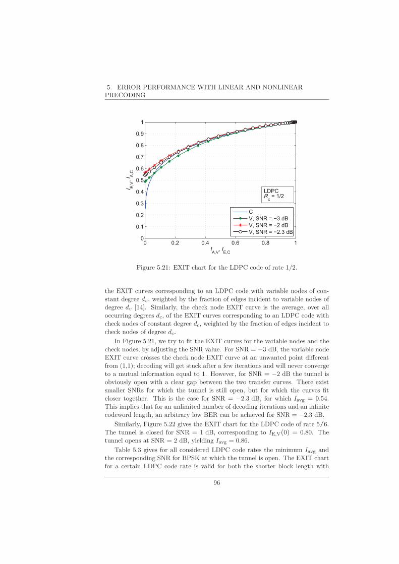
5. ERROR PERFORMANCE WITH LINEAR AND NONLINEARPRECODING
0 0.2 0.4 0.6 0.8 10
0.1
0.2
0.3
0.4
0.5
0.6
0.7
0.8
0.9
1
IA,V
, IE,C
I E,V
,I A
,C
C
V, SNR = �3 dB
V, SNR = �2 dB
V, SNR = �2.3 dB
LDPCR
c = 1/2
Figure 5.21: EXIT chart for the LDPC code of rate 1/2.
the EXIT curves corresponding to an LDPC code with variable nodes of con-stant degree dv, weighted by the fraction of edges incident to variable nodes ofdegree dv [14]. Similarly, the check node EXIT curve is the average, over alloccurring degrees dc, of the EXIT curves corresponding to an LDPC code withcheck nodes of constant degree dc, weighted by the fraction of edges incident tocheck nodes of degree dc.
In Figure 5.21, we try to fit the EXIT curves for the variable nodes and thecheck nodes, by adjusting the SNR value. For SNR = −3 dB, the variable nodeEXIT curve crosses the check node EXIT curve at an unwanted point differentfrom (1,1); decoding will get stuck after a few iterations and will never convergeto a mutual information equal to 1. However, for SNR = −2 dB the tunnel isobviously open with a clear gap between the two transfer curves. There existsmaller SNRs for which the tunnel is still open, but for which the curves fitcloser together. This is the case for SNR = −2.3 dB, for which Iavg = 0.54.This implies that for an unlimited number of decoding iterations and an infinitecodeword length, an arbitrary low BER can be achieved for SNR = −2.3 dB.
Similarly, Figure 5.22 gives the EXIT chart for the LDPC code of rate 5/6.The tunnel is closed for SNR = 1 dB, corresponding to IE,V(0) = 0.80. Thetunnel opens at SNR = 2 dB, yielding Iavg = 0.86.
Table 5.3 gives for all considered LDPC code rates the minimum Iavg andthe corresponding SNR for BPSK at which the tunnel is open. The EXIT chartfor a certain LDPC code rate is valid for both the shorter block length with
96

5.3. LDPC CODES
0 0.2 0.4 0.6 0.8 10
0.1
0.2
0.3
0.4
0.5
0.6
0.7
0.8
0.9
1
IA,V
, IE,C
I E,V
,I A
,C
C
V, SNR = 1 dB
V, SNR = 2 dB
LDPCR
c = 5/6
Figure 5.22: EXIT chart for the LDPC code of rate 5/6.
Table 5.3: SNR and mutual information Iavg for which the tunnel is open in theEXIT chart for all LDPC code rates.
Rc 1/2 2/3 5/6 16/18 20/21
SNR (for BPSK) -2.3 dB -0.1 dB 2 dB 3 dB 5 dBIavg 0.54 0.71 0.86 0.91 0.97
K = 960 and the longer block length with K = 4320 because for a given ratethe longer LDPC codes happen to have the same degree distributions as theshorter LDPC codes at both the variable nodes and the check nodes.
5.3.5 Analysis of Finite-Length LDPC Codes
In Section 5.3.4 we have pointed out that the value of the average mutual in-formation Iavg determines whether the tunnel in the EXIT chart is open, whichindicates whether an infinitely long LDPC code, characterized by its variablenode and check node degree distributions, can achieve an arbitrarily low er-ror probability. By means of simulations, it has been shown in [52] that Iavgalso characterizes the bit error rate (BER) and the word error rate (WER) offinite-length LDPC codes:
• Consider an LDPC code, with all coded bits mapped to a constellation
97

5. ERROR PERFORMANCE WITH LINEAR AND NONLINEARPRECODING
A1 and all resulting constellation symbols operating at SNR = SNR1,which yields Iavg = Iavg,1. Consider the same LDPC code, with all codedbits mapped to a constellation A2 and all resulting constellation symbolsoperating at SNR = SNR2, which yields Iavg = Iavg,2. When SNR2 isadjusted such that Iavg,1 = Iavg,2, than it turns out that the configurations(A1, SNR1) and (A2, SNR2) yield the same BER and the same WER.
• The above result can be generalized to the case where subsets of coded bitsare mapped to different constellations, each operating at different SNRs:configurations yielding the same value of Iavg give rise to the same BERand the same WER.
This powerful result from [52] allows the following analysis method.
• Step 1: We consider the case where all bits from the LDPC code aremapped to a same selected QAM constellation and all resulting constella-tion symbols operate at the same SNR. By means of computer simulations,we determine the BER and WER as a function of SNR.
• Step 2: We make use of the relation between Iavg and SNR for the QAMconstellation selected in step 1 to determine the BER and WER from step1 as a function of Iavg.
• Step 3: Making use of the relations between Iavg and SNR for all 2b-QAMconstellations (b = 1, ..., 12), it is possible to compute Iavg according toSection 5.3.3 for (i) the configuration where the coded bits are mapped toa constellation different from the one selected in step 1 and the resultingconstellations symbols operate at a same SNR; or (ii) even for the moregeneral configuration where subsets of coded symbols are mapped to differ-ent constellations, which operate at different SNRs. Having obtained thevalue of Iavg for the considered configuration, the corresponding BER orWER follows from the relation expressing the BER or WER as a functionof Iavg, derived in step 2.
Hence, in order to determine the error performance for a very wide range of con-figurations mentioned in step 3, we only need for each of the considered LDPCcodes a table containing the BER and WER as a function of SNR for a single
QAM constellation, and for each considered QAM constellation we need a tablecontaining Iavg as a function of SNR. The advantage of this analysis method isthat only a limited number of (time-consuming) LDPC decoder simulations isneeded.
5.3.6 Rule of Thumb
Unlike the cases of uncoded transmission or TCM, for LDPC codes we have noexpression which relates the BER to the minimum distance between the non-
98
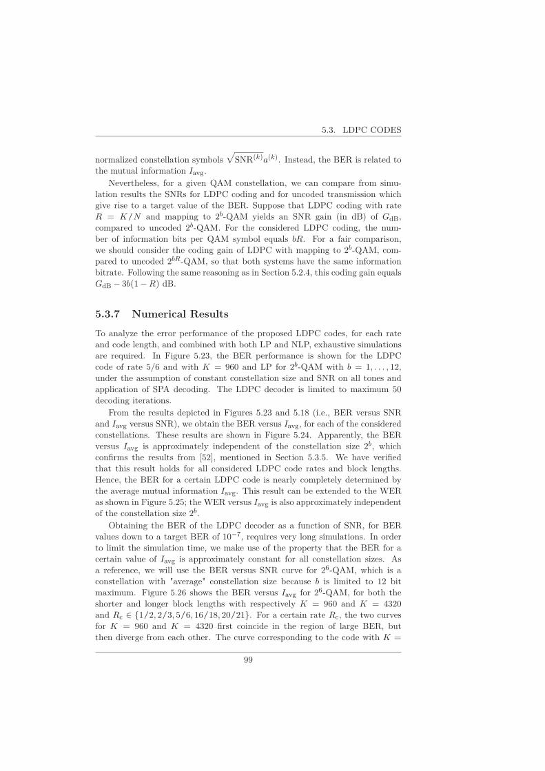
5.3. LDPC CODES
normalized constellation symbols√
SNR(k)a(k). Instead, the BER is related tothe mutual information Iavg.
Nevertheless, for a given QAM constellation, we can compare from simu-lation results the SNRs for LDPC coding and for uncoded transmission whichgive rise to a target value of the BER. Suppose that LDPC coding with rateR = K/N and mapping to 2b-QAM yields an SNR gain (in dB) of GdB,compared to uncoded 2b-QAM. For the considered LDPC coding, the num-ber of information bits per QAM symbol equals bR. For a fair comparison,we should consider the coding gain of LDPC with mapping to 2b-QAM, com-pared to uncoded 2bR-QAM, so that both systems have the same informationbitrate. Following the same reasoning as in Section 5.2.4, this coding gain equalsGdB − 3b(1− R) dB.
5.3.7 Numerical Results
To analyze the error performance of the proposed LDPC codes, for each rateand code length, and combined with both LP and NLP, exhaustive simulationsare required. In Figure 5.23, the BER performance is shown for the LDPCcode of rate 5/6 and with K = 960 and LP for 2b-QAM with b = 1, . . . , 12,under the assumption of constant constellation size and SNR on all tones andapplication of SPA decoding. The LDPC decoder is limited to maximum 50decoding iterations.
From the results depicted in Figures 5.23 and 5.18 (i.e., BER versus SNRand Iavg versus SNR), we obtain the BER versus Iavg, for each of the consideredconstellations. These results are shown in Figure 5.24. Apparently, the BERversus Iavg is approximately independent of the constellation size 2b, whichconfirms the results from [52], mentioned in Section 5.3.5. We have verifiedthat this result holds for all considered LDPC code rates and block lengths.Hence, the BER for a certain LDPC code is nearly completely determined bythe average mutual information Iavg. This result can be extended to the WERas shown in Figure 5.25; the WER versus Iavg is also approximately independentof the constellation size 2b.
Obtaining the BER of the LDPC decoder as a function of SNR, for BERvalues down to a target BER of 10−7, requires very long simulations. In orderto limit the simulation time, we make use of the property that the BER for acertain value of Iavg is approximately constant for all constellation sizes. Asa reference, we will use the BER versus SNR curve for 26-QAM, which is aconstellation with "average" constellation size because b is limited to 12 bitmaximum. Figure 5.26 shows the BER versus Iavg for 26-QAM, for both theshorter and longer block lengths with respectively K = 960 and K = 4320
and Rc ∈ {1/2, 2/3, 5/6, 16/18, 20/21}. For a certain rate Rc, the two curvesfor K = 960 and K = 4320 first coincide in the region of large BER, butthen diverge from each other. The curve corresponding to the code with K =
99

5. ERROR PERFORMANCE WITH LINEAR AND NONLINEARPRECODING
0 10 20 3010
8
10 6
10 4
10 2
100
SNR!(dB)
BER
b = 1
b = 2
b = 3
b = 4
b = 5
b = 6
b = 7
b = 8
b = 9
b = 10
b = 11
b = 12
Figure 5.23: BER performance versus SNR of the LDPC code with Rc = 5/6,K = 960 and LP for constant constellation size, simulations results with SPAdecoding.
0.6 0.7 0.8 0.9 110
�8
10�6
10�4
10�2
100
Iavg
BE
R
b = 1
b = 2
b = 3
b = 4
b = 5
b = 6
b = 7
b = 8
b = 9
b = 10
b = 11
b = 12LDPC withR
c = 5/6
K = 960
Figure 5.24: BER performance versus Iavg of the LDPC code with Rc = 5/6,K = 960 and LP for constant constellation size, simulations results with SPAdecoding.
100

5.3. LDPC CODES
0.6 0.7 0.8 0.9 110
6
10 5
10 4
10 3
10 2
10 1
100
Iavg
WER
b!=!1
b!=!2
b!=!3
b!=!4
b!=!5
b!=!6
b!=!7
b!=!8
b!=!9
b!=!10
b!=!11
b!=!12LDPC!withRc!=!5/6
K!=!960
Figure 5.25: WER performance versus Iavg of the LDPC code with Rc = 5/6,K = 960 and LP for constant constellation size, simulations results with SPAdecoding.
4320 decays more rapidly than the shorter code and has therefore a betterperformance in the region of low BER.
It is interesting to compare Figure 5.26 with Table 5.3, which contains thevalues of Iavg for which the tunnel in the EXIT chart opens. We observe thatthe values of Iavg from Table 5.3 are close to the abscissa of the points wherethe curves in Figure 5.26 for the short codes and the long codes start to diverge.Hence, for a code length growing to infinity, we expect the BER curve to descendvery steeply from a point which is close to the point of divergence observedin Figure 5.26, which is in agreement with this very long code achieving anarbitrary small BER when Iavg exceeds the value indicated in Table 5.3.
Similar to the system with LP, the BER for the system with NLP can beobtained from simulations with SPA decoding. In Figure 5.27, we show resultsversus SNR for a limited number of constellation sizes (b = 1, . . . , 6), under theassumption of constant constellation 2b−QAM and SNR on all tones. As ex-pected, there is a degradation as compared to LP, which decreases for increasingconstellation sizes.
We now combine Figures 5.27 and 5.18, showing respectively the BER versusSNR and Iavg versus SNR, to obtain the BER versus Iavg for the considered con-stellations, which is presented in Figure 5.28. Similar as for LP, we can concludethat the BER versus Iavg for NLP is essentially independent of the constellation
101

5. ERROR PERFORMANCE WITH LINEAR AND NONLINEARPRECODING
0.5 0.6 0.7 0.8 0.9 110
8
10 6
10 4
10 2
100
Iavg
BER
Rc=1/2,K=960
Rc=1/2,K=4320
Rc=2/3,K!=960
Rc=2/3,K=4320
Rc=5/6,K!=960
Rc=5/6,K=4320
Rc=16/18,K!=960
Rc=16/18,K=4320
Rc=20/21,K=960
Rc=20/21,K=4320
Figure 5.26: BER performance versus Iavg of all LDPC codes with K = 960 orK = 4320, Rc ∈ {1/2, 2/3, 5/6, 16/18, 20/21}, LP and 26-QAM, SPA decod-ing.
0 5 10 15 2010
8
10 6
10 4
10 2
100
SNR!(dB)
BER
b !=!1,!LP
b !=!1,!NLP
b !=!2,!LP
b !=!2,!NLP
b !=!3,!LP
b !=!3,!NLP
b !=!4,!LP
b !=!4,!NLP
b !=!5,!LP
b !=!5,!NLP
b !=!6,!LP
b !=!6,!NLP
Figure 5.27: Comparison of the BER performance versus SNR for LP and NLPof the LDPC code with Rc = 5/6 and K = 960, simulations results with SPAdecoding.
102

5.3. LDPC CODES
0.6 0.7 0.8 0.9 110
8
10 6
10 4
10 2
100
Iavg
BER
b !=!1
b !=!2
b !=!3
b !=!4
b !=!5
b !=!6
LDPC!withRc!=!5/6
K!=!960
Figure 5.28: BER performance versus Iavg of the LDPC code with Rc = 5/6,K = 960 and NLP, for constant constellation size, simulations results with SPAdecoding.
size 2b. Moreover, the curves for LP and NLP virtually coincide. The BERperformance of SPA is thus completely determined by Iavg, irrespective of LPor NLP.
From the simulation results performed this far, we derive the value of Iavgwhich is required to achieve BER = 10−7 for both LP and NLP, assuming thesame constellation size M = 2b and the same SNR on all tones. Results aregiven in Table 5.4 for K = 960 and K = 4320. To obtain the SNR values atwhich the required Iavg is achieved, Figures 5.17 and 5.18 should be consultedwhich give the relation between SNR and Iavg for respectively LP and NLP.For the sake of illustration, Table 5.5 shows the SNR values required to achieveBER = 10−7 as a function of the constellation size, for the rate 1/2 LDPC codewith K = 4320 and SMSA decoding, using NLP. For this setting, an increaseof the constellation by 1 bit requires an increase of the SNR by about 2 dB (forlarge constellations) to maintain the same BER. This in is contrast with the ruleof thumb for uncoded transmission and TCM, stating that an increase of theconstellation by 1 bit requires a 3 dB higher SNR. Hence, in general this rule of
thumb does not apply to LDPC codes. This can be understood when assumingthat the LDPC code operates close to the Shannon capacity: in this case, fora rate-Rc code and a 2b-QAM constellation, we have Rcb ≈ log2(1+ SNR) or,equivalently, SNR ≈ 2Rcb − 1, so that increasing b by 1 bit requires SNR toincrease by a factor of about 2Rc , which corresponds to 3Rc dB; for Rc = 1/2,
103

5. ERROR PERFORMANCE WITH LINEAR AND NONLINEARPRECODING
Table 5.4: Required Iavg to achieve the target BER of 10−7 for all proposedLDPC codes with K = 960 and K = 4320 and SPA, with LP and NLP.
Rc 1/2 2/3 5/6 16/18 20/21
K = 960 0.663 0.822 0.946 0.985 0.988K = 4320 0.598 0.764 0.904 0.948 0.985
Table 5.5: Required SNRavg (in dB) to achieve the target BERavg of 10−7 forthe rate 1/2 LDPC code with K = 4320 and SMSA, and NLP.
b 1 2 3 4 5 6
NLP 2.4 4.0 7.2 8.5 10.5 12.4
b 7 8 9 10 11 12
NLP 14.4 16.3 18.5 20.3 22.5 24.3
the resulting SNR increment would be 1.5 dB.
5.4 The Effect of IN
Here we consider the effect of IN on the error performance of the considereduncoded and coded systems with LP and NLP. The IN model and its associatedparameters have been introduced in Section 4.5.
5.4.1 Uncoded Transmission and TCM
5.4.1.1 Detection Algorithm
The detection rules for uncoded transmission ((5.3) for LP and (5.8) for NLP)and TCM ((5.10) for LP and (5.18) for NLP), which have been derived for thecase where IN is absent, are still valid in the presence of IN, provided that
SNR(k) is replaced by the instantaneous SNR, denoted SNR(k)act. This seems to
suggest that the receiver needs to know the instantaneous SNR on each tone, inorder to perform ML detection; however, we will point out that this is not the
case when the instantaneous noise variance N(k)0,act is the same for all tones.
Let us concentrate on the detection of TCM in the case of LP. We havepointed out in Section 4.3 that, for the user considered (user index dropped fornotational convenience), z(k) is a scaled and rotated version of the observation
y(k), i.e., z(k) = y(k) exp(−j arg(L(k)))/√
N(k)0,act, where L(k) and N
(k)0,act are
104

5.4. THE EFFECT OF IN
the diagonal element of L(k) and the instantaneous noise variance, both associ-ated with the considered user. The function DLP(a) from (5.10), with SNR(k)
replaced by SNR(k)act, can be transformed into
DLP(a) =Nt∑
k=1
|L(k)|2E(k)
N(k)0,act
∣∣∣∣∣
y(k)
L(k)√
E(k)− a(k)
∣∣∣∣∣
2
(5.31)
where N(k)0,act = N
(k)0 or N
(k)0,act = N
(k)0 + N0,imp when the DMT symbol interval
is not hit or hit by IN, respectively. Adopting the common assumption that thestationary Gaussian noise n(t) on the channel for the considered user is white,
N(k)0 does not depend on the tone index k, and neither does N
(k)0,act; hence we set
N(k)0 = N0 and N
(k)0,act = N0,act for k = 1, ...,Nt. In this case, removing N0,act
from (5.31) does not affect the ML detection, so we can redefine DLP(a) as
DLP(a) =Nt∑
k=1
|L(k)|2E(k)
∣∣∣∣∣
y(k)
L(k)√
E(k)− a(k)
∣∣∣∣∣
2
(5.32)
Hence, it is sufficient that the receiver knows L(k)√
E(k), and no knowledge
about the instantaneous total noise variance N0,act is needed.
The same reasoning applies to TCMwith NLP, and to uncoded transmission1
(both with LP and NLP). The modifications to be made to the corresponding
decision rules in order to remove N0,act are similar to those for TCM with LP.
5.4.1.2 Error Performance
Let us consider the case where on each tone a 2b-QAM constellation is used,
and all tones have the same value of SNR(k)act, i.e., SNR
(k)act = SNRact. Tak-
ing into account that N(k)0,act does not depend on the tone index, this implies
that |L(k)|2E(k) does not depend on the tone index either, which occurs (for
instance) when the channel transfer function is flat and E(k) does not depend
on the tone index. We set SNRact = SNR when the DMT symbol is not hit
by IN, and SNRact = SNR/(1+ κ) when the DMT symbol is hit by IN, withκ = N0,imp/N0. Hence, the average SNR (i.e., signal power over long-term
average noise power) on each tone is given by SNRavg = SNR/(1+ p1κ), withp1 denoting the steady-state probability that the considered DMT symbol is hit
by IN. The resulting average BER in the presence of IN is given by
BERavg = p0BER(s = 0) + p1BER (s = 1) (5.33)
where p0 = 1− p1, while BER(s = 0) and BER(s = 1) denote the BER forthe considered system (uncoded transmission or TCM, combined with LP or
1For uncoded transmission, it is not needed that N(k)0
is independent of k
105
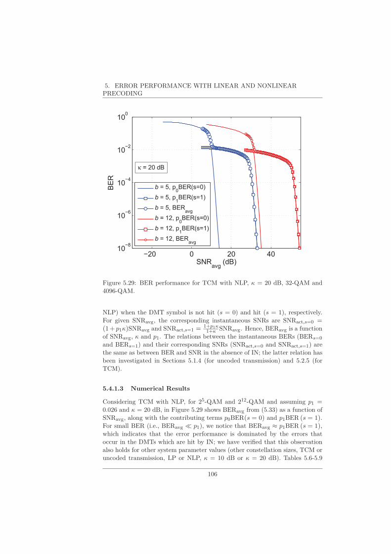
5. ERROR PERFORMANCE WITH LINEAR AND NONLINEARPRECODING
�20 0 20 4010
�8
10�6
10�4
10�2
100
SNRavg
(dB)
BE
R
b = 5, p0BER(s=0)
b = 5, p1BER(s=1)
b = 5, BERavg
b = 12, p0BER(s=0)
b = 12, p1BER(s=1)
b = 12, BERavg
κ = 20 dB
Figure 5.29: BER performance for TCM with NLP, κ = 20 dB, 32-QAM and4096-QAM.
NLP) when the DMT symbol is not hit (s = 0) and hit (s = 1), respectively.For given SNRavg, the corresponding instantaneous SNRs are SNRact,s=0 =(1+ p1κ)SNRavg and SNRact,s=1 =
1+p1κ1+κ SNRavg. Hence, BERavg is a function
of SNRavg, κ and p1. The relations between the instantaneous BERs (BERs=0
and BERs=1) and their corresponding SNRs (SNRact,s=0 and SNRact,s=1) arethe same as between BER and SNR in the absence of IN; the latter relation hasbeen investigated in Sections 5.1.4 (for uncoded transmission) and 5.2.5 (forTCM).
5.4.1.3 Numerical Results
Considering TCM with NLP, for 25-QAM and 212-QAM and assuming p1 =0.026 and κ = 20 dB, in Figure 5.29 shows BERavg from (5.33) as a function ofSNRavg, along with the contributing terms p0BER(s = 0) and p1BER (s = 1).For small BER (i.e., BERavg ≪ p1), we notice that BERavg ≈ p1BER (s = 1),which indicates that the error performance is dominated by the errors thatoccur in the DMTs which are hit by IN; we have verified that this observationalso holds for other system parameter values (other constellation sizes, TCM oruncoded transmission, LP or NLP, κ = 10 dB or κ = 20 dB). Tables 5.6-5.9
106
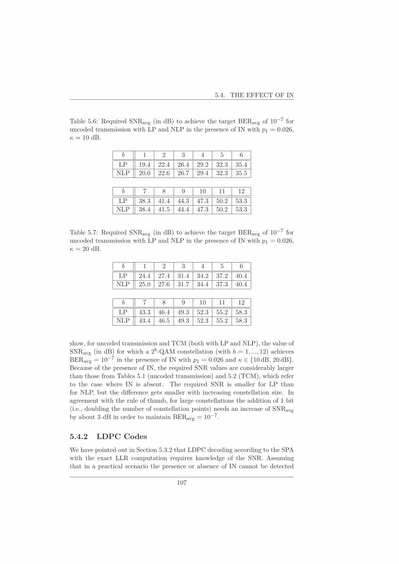
5.4. THE EFFECT OF IN
Table 5.6: Required SNRavg (in dB) to achieve the target BERavg of 10−7 foruncoded transmission with LP and NLP in the presence of IN with p1 = 0.026,κ = 10 dB.
b 1 2 3 4 5 6
LP 19.4 22.4 26.4 29.2 32.3 35.4NLP 20.0 22.6 26.7 29.4 32.3 35.5
b 7 8 9 10 11 12
LP 38.3 41.4 44.3 47.3 50.2 53.3NLP 38.4 41.5 44.4 47.3 50.2 53.3
Table 5.7: Required SNRavg (in dB) to achieve the target BERavg of 10−7 foruncoded transmission with LP and NLP in the presence of IN with p1 = 0.026,κ = 20 dB.
b 1 2 3 4 5 6
LP 24.4 27.4 31.4 34.2 37.2 40.4NLP 25.0 27.6 31.7 34.4 37.3 40.4
b 7 8 9 10 11 12
LP 43.3 46.4 49.3 52.3 55.2 58.3NLP 43.4 46.5 49.3 52.3 55.2 58.3
show, for uncoded transmission and TCM (both with LP and NLP), the value ofSNRavg (in dB) for which a 2b-QAM constellation (with b = 1, ..., 12) achievesBERavg = 10−7 in the presence of IN with p1 = 0.026 and κ ∈ {10 dB, 20 dB}.Because of the presence of IN, the required SNR values are considerably largerthan those from Tables 5.1 (uncoded transmission) and 5.2 (TCM), which referto the case where IN is absent. The required SNR is smaller for LP thanfor NLP, but the difference gets smaller with increasing constellation size. Inagreement with the rule of thumb, for large constellations the addition of 1 bit(i.e., doubling the number of constellation points) needs an increase of SNRavgby about 3 dB in order to maintain BERavg = 10−7.
5.4.2 LDPC Codes
We have pointed out in Section 5.3.2 that LDPC decoding according to the SPAwith the exact LLR computation requires knowledge of the SNR. Assumingthat in a practical scenario the presence or absence of IN cannot be detected
107

5. ERROR PERFORMANCE WITH LINEAR AND NONLINEARPRECODING
Table 5.8: Required SNRavg (in dB) to achieve the target BERavg of 10−7 forTCM with LP and NLP in the presence of IN with p1 = 0.026, κ = 10 dB.
b 1 2 3 4 5 6
LP 13.8 16.8 21.0 24.2 27.4 30.6NLP 15.5 17.7 21.7 24.7 27.5 30.8
b 7 8 9 10 11 12
LP 33.5 36.7 39.6 42.8 45.6 48.8NLP 33.7 36.9 39.7 42.8 45.6 48.8
Table 5.9: Required SNRavg (in dB) to achieve the target BERavg of 10−7 forTCM with LP and NLP in the presence of IN with p1 = 0.026, κ = 20 dB.
b 1 2 3 4 5 6
LP 18.8 21.8 26.0 29.2 32.3 35.6NLP 20.5 22.7 26.7 29.6 32.5 35.8
b 7 8 9 10 11 12
LP 38.5 41.7 44.6 47.7 50.6 53.7NLP 38.7 41.8 44.7 47.8 50.6 53.8
108

5.4. THE EFFECT OF IN
for each individual DMT symbol, the instantaneous SNR is not known to thereceiver. One could still perform LDPC decoding using the average SNR insteadof the instantaneous SNR; however, in this case the decoder is a "mismatched"(i.e., operating at an SNR which is different from the assumed SNR), yieldingan error performance degradation. Therefore we consider here LDPC decodingaccording to the (S)MSA (see Sections 2.3.1.2 and 2.3.1.3) with the approximateLLR computation, which does not require knowledge of the instantaneous SNRat the receiver.
5.4.2.1 Approximate LLRs
In the case of LP, the approximate LLR messages (2.7) in the MSA and SMSAdecoding algorithm from respectively Sections 2.3.1.2 and 2.3.1.3 are computedas
Lch→n = mina(k)∈A(k)
cn=1
∣∣∣y(k) − L(k)
√
E(k)a(k)∣∣∣
2
− mina(k)∈A(k)
cn=0
∣∣∣y(k) − L(k)
√
E(k)a(k)∣∣∣
2
(5.34)
with y(k) from (4.21). In the case of NLP, y(k) is given by (4.30), so that A(k)cn=0
and A(k)cn=1
in (5.34) must be replaced by their extended constellations A(k)ext,cn=0
and A(k)ext,cn=1
.The approximate LLRs serve as input to the decoding algorithms from Sec-
tions 2.3.1.2 and 2.3.1.3 for respectively MSA and SMSA.
5.4.2.2 Error Performance
For the error performance analysis of the LDPC codes in the presence of IN wefollow the same reasoning as for uncoded transmission and TCM, outlined in5.4.1.2.
Considering the case where on each tone a 2b-QAM constellation is used,
and all tones have the same value of SNR(k)act, i.e., SNR
(k)act = SNRact, the ex-
pression (5.33) also holds in the case of LDPC codes. The relations betweenthe instantaneous BERs (BERs=0 and BERs=1) and their corresponding SNRs(SNRact,s=0 and SNRact,s=1) are the same as between BER and SNR in theabsence of IN. The latter relation has been investigated in Section 5.3.7, butonly for decoding according to the SPA with exact LLRs. In Section 5.4.2.3 wewill verify that the performance analysis method outlined in Section 5.3.5 stillapplies for decoding by means of the (S)MSA with approximated LLRs.
5.4.2.3 Numerical Results
First, we investigate for the approximate LLRs the relation between the averagemutual information Iavg and the instantaneous SNR, for various constellations.
For the approximate LLRs, the mutual information I(c(k)j ,L
(k)j ) from (5.30)
109
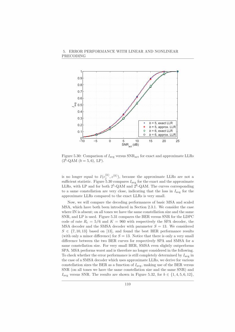
5. ERROR PERFORMANCE WITH LINEAR AND NONLINEARPRECODING
�10 �5 0 5 10 15 20 250
0.1
0.2
0.3
0.4
0.5
0.6
0.7
0.8
0.9
1
SNRact
(dB)
I avg
b = 5, exact LLR
b = 5, approx. LLR
b = 6, exact LLR
b = 6, approx. LLR
Figure 5.30: Comparison of Iavg versus SNRact for exact and approximate LLRs(2b-QAM (b = 5, 6), LP).
is no longer equal to I(c(k)j , z(k)), because the approximate LLRs are not a
sufficient statistic. Figure 5.30 compares Iavg for the exact and the approximate
LLRs, with LP and for both 25-QAM and 26-QAM. The curves corresponding
to a same constellation are very close, indicating that the loss in Iavg for the
approximate LLRs compared to the exact LLRs is very small.
Now, we will compare the decoding performances of basic MSA and scaled
MSA, which have both been introduced in Section 2.3.1. We consider the case
where IN is absent; on all tones we have the same constellation size and the same
SNR, and LP is used. Figure 5.31 compares the BER versus SNR for the LDPC
code of rate Rc = 5/6 and K = 960 with respectively the SPA decoder, the
MSA decoder and the SMSA decoder with parameter S = 13. We considered
S ∈ {7, 10, 13} based on [13], and found the best BER performance results(with only a minor difference) for S = 13. Notice that there is only a very small
difference between the two BER curves for respectively SPA and SMSA for a
same constellation size. For very small BER, SMSA even slightly outperforms
SPA. MSA performs worst and is therefore no longer considered in the following.
To check whether the error performance is still completely determined by Iavg in
the case of a SMSA decoder which uses approximate LLRs, we derive for various
constellation sizes the BER as a function of Iavg, making use of the BER versus
SNR (on all tones we have the same constellation size and the same SNR) and
Iavg versus SNR. The results are shown in Figure 5.32, for b ∈ {1, 4, 5, 6, 12},
110

5.4. THE EFFECT OF IN
0 2 4 6 8 10 12 14 16 1810
8
10 6
10 4
10 2
100
SNR!(dB)
BER
b !=!1,!SPA
b !=!1,!MSA
b !=!1,!SMSA!S!=!13
b !=!4,!SPA
b !=!4,!MSA
b !=!4,!SMSA!S!=!13
b !=!5,!SPA
b !=!5,!MSA
b !=!5,!SMSA!S!=!13
Figure 5.31: Comparison of the BER performance versus SNR for the LDPCcode of rate Rc = 5/6, K = 960 and LP with respectively SPA decoder, MSAdecoder and SMSA decoder, simulations results.
assuming a rate 5/6 LDPC code with K = 960 and using LP. We observe thatthe BER versus Iavg is still approximately independent of the constellation size2b, indicating the validity of the analysis method from Section 5.3.5 also forLDPC decoding with SMSA and approximate LLRs.
Table 5.10 shows the value of Iavg which is required to achieve BER = 10−7
for all proposed LDPC codes with K = 960 and K = 4320, and SMSA withS = 13 and approximate LLRs for both LP and NLP. Comparing with Table5.4 which holds for SPA with exact LLRs, we see that SMSA for most codeconfigurations requires a slightly lower Iavg; this confirms the better performanceat BER = 10−7 for SMSA compared to SPA, observed in Figure 5.31 for therate 5/6 code with K = 960.
Having verified the validity of the analysis method from Section 5.3.5 forSMSA with approximate LLRs, we have used this method to determine BERavg
versus SNRavg in the presence of IN (on all tones we have the same constellationsize and the same instantaneous SNR), based on (5.33). As an illustration,Table 5.11 gives the required SNRavg values for the rate 20/21 LDPC code withK = 4320 and SMSA decoding (S = 13) to achieve target BERavg equal to10−7. We consider both LP and NLP. Furthermore, IN of levels κ = −∞ (i.e.,no IN), 10 dB and 20 dB are considered. We observe that LP outperformsNLP in terms of SNRavg but the difference in performance becomes negligiblefor large constellations. The stronger the IN, the larger the value of SNRavg
111

5. ERROR PERFORMANCE WITH LINEAR AND NONLINEARPRECODING
0.6 0.7 0.8 0.9 110
8
10 6
10 4
10 2
100
Iavg
BER
b!=!1
b!=!4
b!=!5
b!=!6
b!=!12
LDPC!withRc!=!5/6
K!=!960
Figure 5.32: BER performance versus Iavg of the LDPC code with Rc = 5/6,K = 960 and LP for constant constellation size, simulations results with SMSAdecoding.
needed to maintain BERavg = 10−7.
5.5 Interleaving against IN
The combination of interleaving with FEC is a means to counteract burst errorscaused by IN.
In the arrangement shown in Figure 5.33, a number of codewords are col-lected at the output of the FEC encoder, and applied to the interleaver. Theinterleaver performs a random permutation on ’parts’ (bits, bytes, constellationsymbols) of the codeword, and the output of the interleaver is sent over the chan-
Table 5.10: Required Iavg to achieve the target BER of 10−7 for all proposedLDPC codes with K = 960 and K = 4320, and SMSA with S = 13, for bothLP and NLP.
Rc 1/2 2/3 5/6 16/18 20/21
K = 960 0.649 0.805 0.931 0.975 0.996K = 4320 0.596 0.759 0.893 0.939 0.982
112
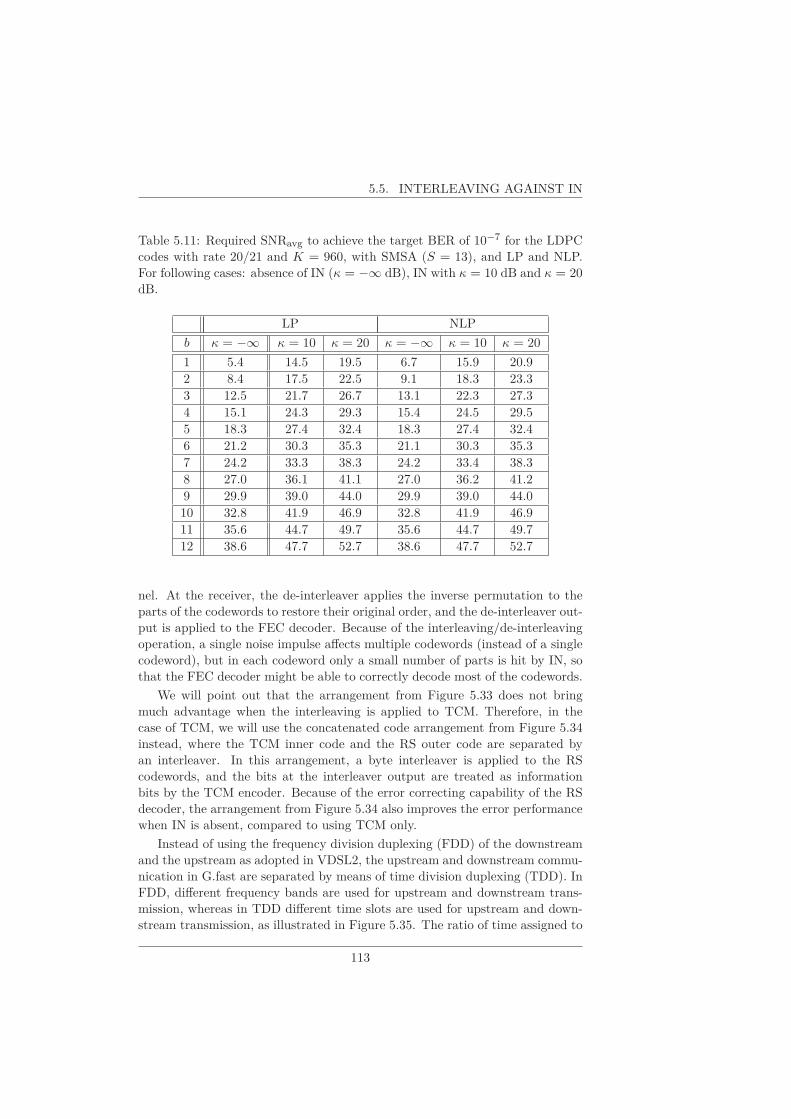
5.5. INTERLEAVING AGAINST IN
Table 5.11: Required SNRavg to achieve the target BER of 10−7 for the LDPCcodes with rate 20/21 and K = 960, with SMSA (S = 13), and LP and NLP.For following cases: absence of IN (κ = −∞ dB), IN with κ = 10 dB and κ = 20
dB.
LP NLP
b κ = −∞ κ = 10 κ = 20 κ = −∞ κ = 10 κ = 20
1 5.4 14.5 19.5 6.7 15.9 20.92 8.4 17.5 22.5 9.1 18.3 23.33 12.5 21.7 26.7 13.1 22.3 27.34 15.1 24.3 29.3 15.4 24.5 29.55 18.3 27.4 32.4 18.3 27.4 32.46 21.2 30.3 35.3 21.1 30.3 35.37 24.2 33.3 38.3 24.2 33.4 38.38 27.0 36.1 41.1 27.0 36.2 41.29 29.9 39.0 44.0 29.9 39.0 44.010 32.8 41.9 46.9 32.8 41.9 46.911 35.6 44.7 49.7 35.6 44.7 49.712 38.6 47.7 52.7 38.6 47.7 52.7
nel. At the receiver, the de-interleaver applies the inverse permutation to theparts of the codewords to restore their original order, and the de-interleaver out-put is applied to the FEC decoder. Because of the interleaving/de-interleavingoperation, a single noise impulse affects multiple codewords (instead of a singlecodeword), but in each codeword only a small number of parts is hit by IN, sothat the FEC decoder might be able to correctly decode most of the codewords.
We will point out that the arrangement from Figure 5.33 does not bringmuch advantage when the interleaving is applied to TCM. Therefore, in thecase of TCM, we will use the concatenated code arrangement from Figure 5.34instead, where the TCM inner code and the RS outer code are separated byan interleaver. In this arrangement, a byte interleaver is applied to the RScodewords, and the bits at the interleaver output are treated as informationbits by the TCM encoder. Because of the error correcting capability of the RSdecoder, the arrangement from Figure 5.34 also improves the error performancewhen IN is absent, compared to using TCM only.
Instead of using the frequency division duplexing (FDD) of the downstreamand the upstream as adopted in VDSL2, the upstream and downstream commu-nication in G.fast are separated by means of time division duplexing (TDD). InFDD, different frequency bands are used for upstream and downstream trans-mission, whereas in TDD different time slots are used for upstream and down-stream transmission, as illustrated in Figure 5.35. The ratio of time assigned to
113
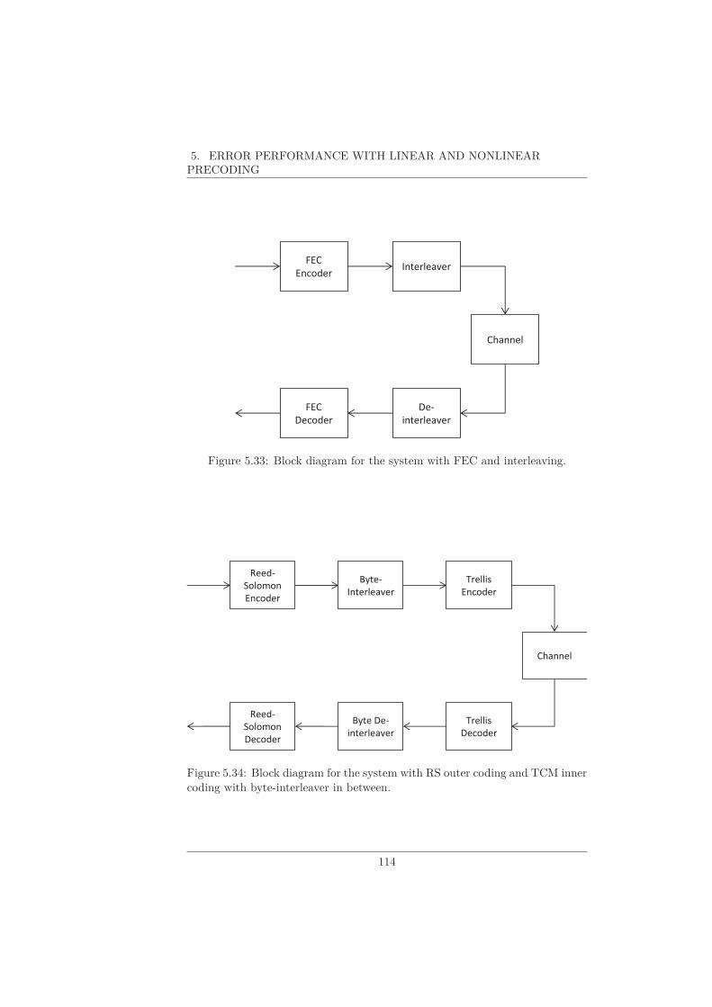
5. ERROR PERFORMANCE WITH LINEAR AND NONLINEARPRECODING
FEC
Decoder
FEC
Encoder Interleaver
Channel
De-
interleaver
Figure 5.33: Block diagram for the system with FEC and interleaving.
Reed-
Solomon
Decoder
Reed-
Solomon
Encoder
Byte-
Interleaver
Trellis
Encoder
Channel
Byte De-
interleaver
Trellis
Decoder
Figure 5.34: Block diagram for the system with RS outer coding and TCM innercoding with byte-interleaver in between.
114

5.5. INTERLEAVING AGAINST IN
1st TDD cycle 2nd TDD cycle
Transmitter
Receiver
t
t s�375
Figure 5.35: TDD cycle with 50% upstream and 50% downstream traffic.
the upstream and the downstream in G.fast is flexible, any ratio between 90%
down/10% up and 30% down/70% up can be configured [53]. In our study, the
TDD frame (including upstream and downstream DMT symbols) has a duration
TTDD = 750 µs and an equal ratio (50%) of the TDD frame is assigned to up-
stream and downstream traffic. With a DMT symbol rate of 48000 symbols/s,
36 DMT symbols can be transmitted during a TDD frame of 750 µs. One DMT
symbol period is reserved as gap [42] and not used to transmit a DMT symbol.
18 DMTs are transmitted during a downstream time slot of 375 µs followed by
17 DMTs which are transmitted during the next upstream time slot.
A major drawback of interleaving is that it adds latency, as the receiver has to
wait until all interleaved symbols are received before deinterleaving and further
processing can start. When interleaving occurs over J downstream slots, the
latency amounts to J downstream slots plus J − 1 upstream slots. In order to
avoid the contribution of upstream slots to the latency, the interleaving should
be limited to a single downstream slot.
Let us assume that as a result of interleaving, an interleaved codeword con-
tains bits from L consecutive DMT symbols, with time indices l, l + 1, . . . , l +L − 1. A DMT symbol with time index l is characterized by a state sl which
indicates whether the DMT is hit (sl = 1) or not hit (sl = 0) by IN with
statistics as described in Section 4.5. Representing the conditional BER and
WER after decoding the considered codeword as BER(sl) and WER(sl) withsl = (sl, sl+1, . . . , sl+L−1), the average BER and WER after decoding are givenby BERavg = E [BER(sl)] and WERavg = E [WER(sl)], where the expectionis over the state vector sl; the probability of sl follows easily from the 2-state
Markov IN model.
115

5. ERROR PERFORMANCE WITH LINEAR AND NONLINEARPRECODING
5.5.1 TCM + tone-interleaving
We consider the case where the QAM symbols of a TCM codeword are inter-leaved over L DMT symbols, and LP is used. Let us assume that, as a result ofthe interleaving/de-interleaving operation, n of the Nt symbols of the codewordoriginate from DMT symbols which are hit by IN, while the remaining Nt − n
symbols originate from DMT symbols which are not hit by IN. The most likelydecoding errors involve codewords at minimum distance 2d from the correctcodeword, which differ from the correct codeword only at QAM symbol posi-tions which are hit by IN. In Section 5.2.2 we have shown that these codewordsat distance 2d differ from the correct codeword in only one trellis section (i.e.,they represent parallel transitions). As it is more likely that only one QAMsymbol from a trellis section is hit by IN, we will ignore the probability thatboth QAM symbols from a same trellis section are affected by IN. Consideringdecoding errors involving only one QAM symbol error, it follows from Section5.2.2 that there exist 4 parallel transitions at distance 2d for a given QAMsymbol position. Assuming that on average half of the log2(M )− 1/2 informa-tion bits associated with the erroneous QAM symbol are in error, the resultingapproximation of the average BER is
BERavg ≈ 2E[n]
NtQ
(√
2d2SNRavg1+ p1κ
1+ κ
)
= 2p1Q
(√
2d2SNRavg1+ p1κ
1+ κ
)
(5.35)
where we have taken into account that E[n] = p1Nt.
When no interleaving is used, the BER follows from (5.33). Keeping onlythe second term, we obtain
BERavg ≈ 12p1Q
(√
2d2SNRavg1+ p1κ
1+ κ
)
(5.36)
Comparing (5.35) and (5.36), we conclude that tone-interleaving of the TCMcodeword reduces the BER only by a factor of about 6, compared to no inter-leaving. This rather poor performance in the presence of interleaving is dueto the existence of codewords at minimum distance involving only one QAMsymbol error.
For tone-interleaved TCM with NLP, similar conclusions can be drawn: theuse of interleaving does not improve the argument of the function Q(.) in theBER expression, but only somewhat reduces the factor in front of the functionQ(.).
116

5.5. INTERLEAVING AGAINST IN
5.5.2 RS + byte-interleaver + TCM
Considering the very limited error performance gain achieved by applying tone-interleaving to the TCM codewords, DSL transmission typically makes use ofthe arrangement from Figure 5.34, involving the concatenation of a RS outercode and TCM as inner code, with byte-interleaving (transmitter side) andbyte-de-interleaving (receiver side) in between the two encoders and decoders,respectively. At the receiver, first Viterbi decoding of the TCM is performed,next the resulting bytes are de-interleaved and supplied to the RS decoder forpossible correction of remaining errors. The byte interleaver is introduced tocounteract the burstiness of byte errors at the TCM decoder output. Section5.5.2.1 presents the error performance analysis of this system and numericalresults are presented in Section 5.5.2.2.
5.5.2.1 Performance Analysis
The RS code used in G.fast [42] is defined over the Galois field GF(28), wherea RS code symbol consists of 1 byte (q = 8 bits). Per block of K informa-tion bytes, an additional N − K parity bytes are transmitted. The value of N
can vary from 32 to 255, and N − K must be one of the values from the set{2, 4, 6, 8, 10, 12, 14, 16}. This RS(N ,K) code is systematic and can correct upto
t =
⌊N − K
2
⌋
(5.37)
byte errors.Taking into account the considerations about the interleaver depth in Section
5.5, we briefly discuss the case where RS codewords are interleaved over 18DMT symbols (i.e., within one downstream slot of 375 µs). Assuming the useof the traditional RS(255,239) code (which can correct up to 8 byte errors) anddistributing the bytes of the RS codewords evenly over the 18 DMT symbols,each DMT contains either
⌊25518
⌋= 14 or
⌊25518
⌋+ 1 = 15 bytes from a given RS
codeword. When only one of the 18 DMT symbols is hit by IN, then in each ofthe RS codewords contained within the downstream slot there are 14 or 15 byteshit by IN. When the IN is strong, these bytes are likely to be erroneous. As theRS code can correct only up to 6 byte errors, none of these RS codewords can becorrectly decoded. Hence, interleaving over only 18 DMT symbols does not givemuch protecion against IN. As a matter of fact, the situation with interleavingis even worse than without interleaving, because in the former case the numberof undecodable RS codewords is 18 times as large as in the latter (assuming onlyone of the 18 DMT symbols is hit by IN). From this brief analysis it follows thatinterleaving within a single downstream slot is not sufficient to provide adequate
protection against IN.
As explained in the beginning of Section 5.5, interleaving over multiple
downstream slots would considerably increase the latency for each codeword.
117

5. ERROR PERFORMANCE WITH LINEAR AND NONLINEARPRECODING
Therefore, in this dissertation we will instead focus on a different technique tocounteract IN, i.e., the use of retransmission protocols (see Section 5.6). As faras interleaving (without ARQ) is concerned, we will restrict our attention to thetraditional concatenation of a RS outer code and TCM inner code; we will con-sider the limiting case of infinite interleaving, which provides a lower bound onthe error probability, to which the actual error probability will converge whenthe interleaving depth increases (at the expense of growing latency).
The input of the RS decoder is the byte de-interleaved output of the TCMViterbi decoder. We assume an infinitely large interleaver, such that the byteerrors in the RS codeword can be considered to occur independently with a byteerror probability Pbyte,avg, where Pbyte,avg denotes the average byte error rateat the TCM decoder output. Similar to (5.33), Pbyte,avg is the average of thebyte error rates corresponding to DMT symbol intervals which are hit and nothit by IN, respectively. When all tones of the TCM codeword carry the sameconstellation and have the same SNR, an approximation of the byte error rateat the TCM decoder output in the absence of IN can be obtained in a similarway as the BER approximation (5.16); we obtain
ByteER ≈ 24Q(√
2d2SNR)
(5.38)
where the factor in front of Q(.) results from the simplifying assumption that(i) a trellis section contains an integer number of information bytes; and (ii) allbytes associated with an erroneous trellis section are in error. In the presence ofIN, we must replace in (5.38) SNR by SNRavg
1+p1κ1+κ or SNRavg(1+ p1κ), when
the considered DMT symbol is hit by IN or not hit, respectively.The error performance of the RS decoder solely depends on the RS code
parameters t and N , and on the average byte error probability Pbyte,avg afterTCM Viterbi decoding. The corresponding RS decoding error probability Pe,RSand the byte error rate ByteERRS at the RS decoder output are given by (2.11)and (2.12). The BER after RS decoding is then approximated as
BERRS ≈ 1
2ByteERRS (5.39)
assuming that on average half the bits of an erroneous byte are in error.
5.5.2.2 Numerical Results
We consider two RS codes: the traditional RS(255,239) code and the shortenedRS(136,120) code with an information block length equal to the informationblock length of the shorter LDPC codes (120 bytes = 960 bits). For both RScodes, 16 parity bytes are added which implies that up to t = 8 erroneous bytescan be corrected.
First we consider the byte error rate at the TCM decoder output, in theabsence of IN. Figure 5.36 shows ByteER for LP, constant SNR and the same
118

5.5. INTERLEAVING AGAINST IN
0 10 20 30 4010
8
10 6
10 4
10 2
100
SNR!(dB)
ByteER
b!=!1
b!=!2
b!=!3
b!=!4
b!=!5
b!=!6
b!=!7
b!=!8
b!=!9
b!=!10
b!=!11
b!=!12
Figure 5.36: Simulated (solid line with markers) and approximate (dashed line)ByteER at TCM decoder output for LP with b-bit QAM constellations (b =1, . . . , 12).
QAM constellations on all tones with b = 1, . . . , 12. The solid lines and dashedlines correspond to the simulations and the approximation (5.38) respectively.The analytical approximation is less accurate for small constellation sizes, wheremultiple tone pairs are needed to transmit a single byte of information bits.Therefore, in the sequel we take ByteER equal to the simulation result.
Figure 5.37 compares for 26-QAM and LP several error rates versus SNR(same SNR on all tones) in the absence of IN: the BER for uncoded transmis-sion, the BER and ByteER for TCM, and the BER for the concatenation ofthe RS(255,239) and RS(136,120) outer code and the TCM inner code, withinfinite byte-interleaving. The considered coding schemes bring a substantialperformance improvement w.r.t. uncoded transmission. Note, however, thatthe number of information bits per QAM symbol is different for the consid-ered schemes: for uncoded transmission, TCM only, RS(255,239)+TCM andRS(136,120)+TCM, the number of information bits per QAM symbol equals 6,5.5, 5.5 · 239/255 = 5.15 and 5.5 · 120/136 = 4.85, respectively. In order to have6 information bits per QAM symbol also for the coded systems, their constel-lation sizes should be increased to (on average) 6.5, 6.9 and 7.3 bits (i.e., infobits+parity bits) for TCM only, RS(255,239)+TCM and RS(136,120)+TCM, in
119

5. ERROR PERFORMANCE WITH LINEAR AND NONLINEARPRECODING
18 20 22 24 26 2810
8
10 6
10 4
10 2
100
SNR!(dB)
BER!uncoded
BER!TCM
Pbyte
TCM
BER RS(255,239)
BER RS(139,120)
Figure 5.37: Comparison of error performance versus SNR for LP, 26-QAM anduncoded transmission, TCM, RS(255,239) and RS(136,120).
which case the coding gains observed from Figure 5.37 should be decreased byabout 1.5 dB, 2.7 dB and 3.9 dB, according to the rule of thumb from Section5.2.4.
In Figure 5.38, the BER performance in the absence of IN is shown for bothRS(255,239) + byte-interleaver + TCM and RS(136,120) + byte-interleaver +TCM versus SNR with LP; all tones have the same SNR and the same 2b-QAM constellation, with b = 1, . . . , 12. For each constellation size the fig-ures shows two curves: the solid line gives the BER for the concatenated codewith RS(255,239), the dashed line corresponds to the concatenated code withRS(136,120); only a minor difference (in favor of the shorter RS code) is visibleon this scale between each two curves corresponding to the same constellationsize. Similar figures can be obtained for RS + byte-interleaver + TCM withNLP, but are not shown here for conciseness.
We have investigated the BER performance of the concatenation of RS andTCM with infinite byte-interleaving, operating on (5.1) for LP and on (5.2)for NLP, assuming that the constellation size and the SNR are the same forall tones. Table 5.12 shows, for 2b-QAM, the SNR values that are required toachieve BER = 10−7 in the absence of IN, for the two considered concatenatedcodes with RS(255,239) and RS(136,120). Tables 5.13 and 5.14 show similar
120
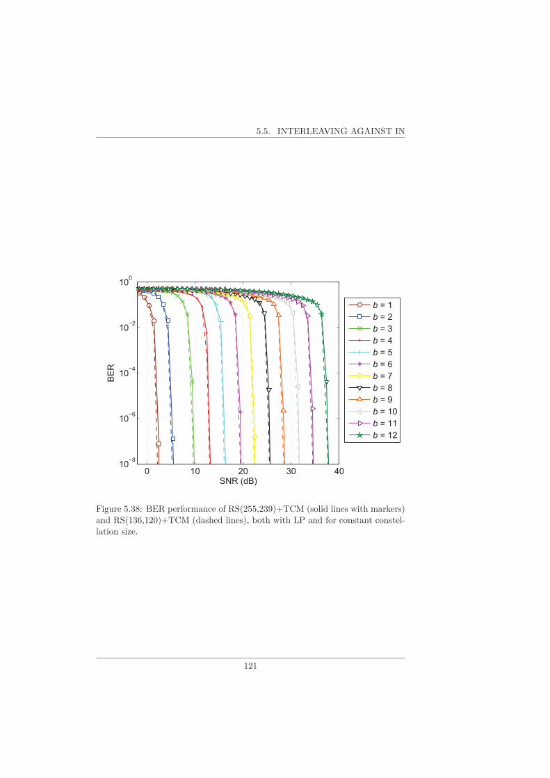
5.5. INTERLEAVING AGAINST IN
0 10 20 30 4010
8
10 6
10 4
10 2
100
SNR!(dB)
BER
b!=!1
b!=!2
b!=!3
b!=!4
b!=!5
b!=!6
b!=!7
b!=!8
b!=!9
b!=!10
b!=!11
b!=!12
Figure 5.38: BER performance of RS(255,239)+TCM (solid lines with markers)and RS(136,120)+TCM (dashed lines), both with LP and for constant constel-lation size.
121

5. ERROR PERFORMANCE WITH LINEAR AND NONLINEARPRECODING
Table 5.12: Required SNR (in dB) to achieve the target BER of 10−7 for RS +byte-interleaver + TCM with LP and NLP.
b 1 2 3 4 5 6
RS(255,239)LP 2.4 5.4 9.7 13.1 16.2 19.5NLP 4.7 6.7 10.7 13.6 16.5 19.8
RS(136,120)LP 2.2 5.2 9.5 12.9 16.1 19.4NLP 4.6 6.6 10.5 13.5 16.3 19.6
b 7 8 9 10 11 12
RS(255,239)LP 22.5 25.6 28.6 31.7 34.5 37.7NLP 22.6 25.8 28.6 31.8 34.5 37.8
RS(136,120)LP 22.3 25.5 28.4 31.6 34.4 37.5NLP 22.4 25.6 28.4 31.6 34.4 37.6
results pertaining to SNRavg for RS + byte-interleaver + TCM, now in thepresence of IN with κ = 10 dB and κ = 20 dB, respectively. From thesetables we observe that the SNR difference between LP and NLP for the sameb is larger as compared to the system with only TCM (see Tables 5.8 and 5.9),especially for small b; this can be explained by noticing that in the concatenatedarrangement the trellis decoder operates at a much smaller SNR (higher errorrate) than in the case where only TCM is used, and that the degradation, interms of SNR, of the trellis decoder performance for NLP compared to LPincreases with increasing error rate. The concatenation involving the shorterRS code slightly outperforms the concatenation involving the longer RS code;both codes have the same error correcting capability, but for the longer codethere are more error patterns containing a given number of byte errors. Forlarge constellations, doubling the constellation size (i.e., increasing b by one bit)requires an increase of the SNR by about 3 dB to maintain the BER value at10−7, which is in agreement with the rule of thumb.
5.6 Use of ARQ against IN
In the presence of IN, our system can benefit from the addition of ARQ, asdepicted in the block diagram in Figure 5.39. The receiver is able to requestthe retransmission of a packet or data transfer unit (DTU) that has been erro-neously received by sending a negative acknowledgment (NAK) message to thetransmitter. The occurrence of an occasional large noise impulse will typicallyaffect several consecutive DTUs and result in a burst of DTU errors. This canbe handled by ARQ; if the cyclic redundancy check (CRC) in the header ofthe DTU fails, the receiver will ask for a retransmission and the transmitter
122
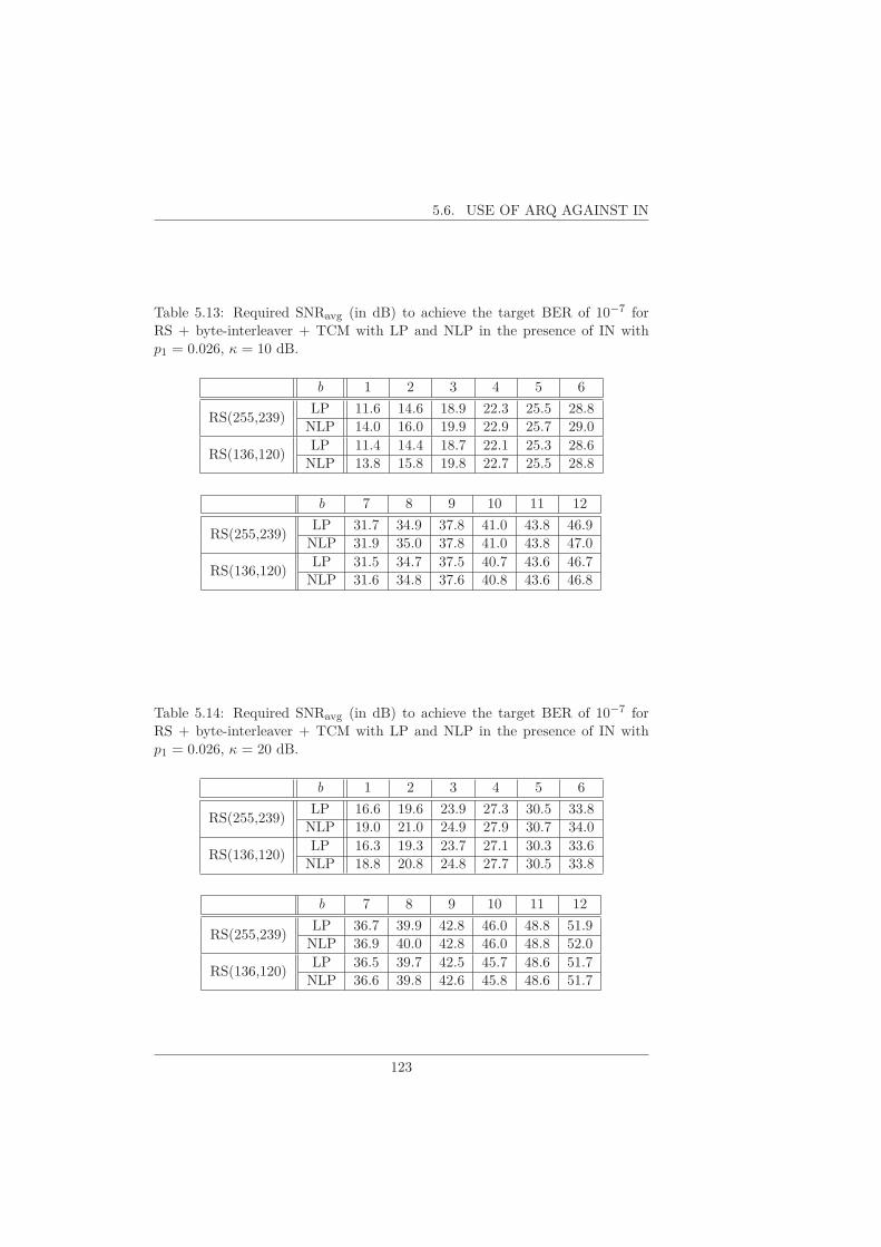
5.6. USE OF ARQ AGAINST IN
Table 5.13: Required SNRavg (in dB) to achieve the target BER of 10−7 forRS + byte-interleaver + TCM with LP and NLP in the presence of IN withp1 = 0.026, κ = 10 dB.
b 1 2 3 4 5 6
RS(255,239)LP 11.6 14.6 18.9 22.3 25.5 28.8NLP 14.0 16.0 19.9 22.9 25.7 29.0
RS(136,120)LP 11.4 14.4 18.7 22.1 25.3 28.6NLP 13.8 15.8 19.8 22.7 25.5 28.8
b 7 8 9 10 11 12
RS(255,239)LP 31.7 34.9 37.8 41.0 43.8 46.9NLP 31.9 35.0 37.8 41.0 43.8 47.0
RS(136,120)LP 31.5 34.7 37.5 40.7 43.6 46.7NLP 31.6 34.8 37.6 40.8 43.6 46.8
Table 5.14: Required SNRavg (in dB) to achieve the target BER of 10−7 forRS + byte-interleaver + TCM with LP and NLP in the presence of IN withp1 = 0.026, κ = 20 dB.
b 1 2 3 4 5 6
RS(255,239)LP 16.6 19.6 23.9 27.3 30.5 33.8NLP 19.0 21.0 24.9 27.9 30.7 34.0
RS(136,120)LP 16.3 19.3 23.7 27.1 30.3 33.6NLP 18.8 20.8 24.8 27.7 30.5 33.8
b 7 8 9 10 11 12
RS(255,239)LP 36.7 39.9 42.8 46.0 48.8 51.9NLP 36.9 40.0 42.8 46.0 48.8 52.0
RS(136,120)LP 36.5 39.7 42.5 45.7 48.6 51.7NLP 36.6 39.8 42.6 45.8 48.6 51.7
123
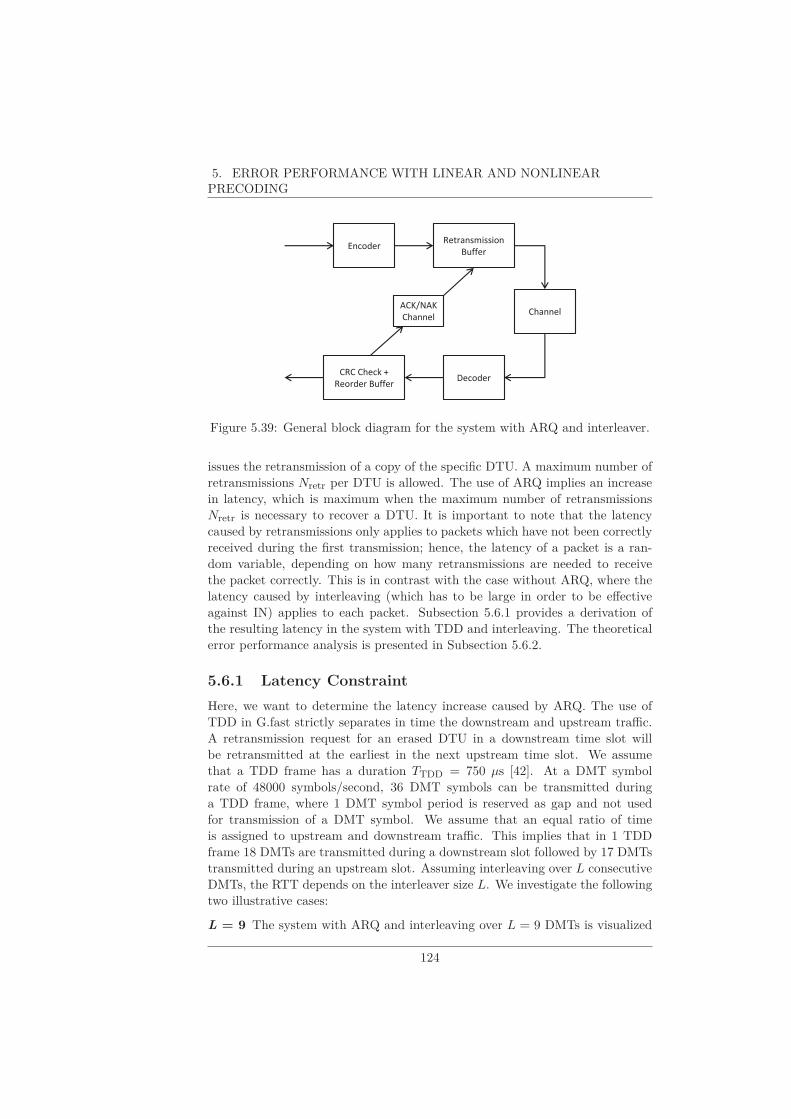
5. ERROR PERFORMANCE WITH LINEAR AND NONLINEARPRECODING
Encoder Retransmission
Buffer
Channel
CRC Check +
Reorder Buffer Decoder
ACK/NAK
Channel
Figure 5.39: General block diagram for the system with ARQ and interleaver.
issues the retransmission of a copy of the specific DTU. A maximum number ofretransmissions Nretr per DTU is allowed. The use of ARQ implies an increasein latency, which is maximum when the maximum number of retransmissionsNretr is necessary to recover a DTU. It is important to note that the latencycaused by retransmissions only applies to packets which have not been correctlyreceived during the first transmission; hence, the latency of a packet is a ran-dom variable, depending on how many retransmissions are needed to receivethe packet correctly. This is in contrast with the case without ARQ, where thelatency caused by interleaving (which has to be large in order to be effectiveagainst IN) applies to each packet. Subsection 5.6.1 provides a derivation ofthe resulting latency in the system with TDD and interleaving. The theoreticalerror performance analysis is presented in Subsection 5.6.2.
5.6.1 Latency Constraint
Here, we want to determine the latency increase caused by ARQ. The use ofTDD in G.fast strictly separates in time the downstream and upstream traffic.A retransmission request for an erased DTU in a downstream time slot will
be retransmitted at the earliest in the next upstream time slot. We assume
that a TDD frame has a duration TTDD = 750 µs [42]. At a DMT symbol
rate of 48000 symbols/second, 36 DMT symbols can be transmitted during
a TDD frame, where 1 DMT symbol period is reserved as gap and not used
for transmission of a DMT symbol. We assume that an equal ratio of time
is assigned to upstream and downstream traffic. This implies that in 1 TDD
frame 18 DMTs are transmitted during a downstream slot followed by 17 DMTs
transmitted during an upstream slot. Assuming interleaving over L consecutive
DMTs, the RTT depends on the interleaver size L. We investigate the following
two illustrative cases:
L = 9 The system with ARQ and interleaving over L = 9 DMTs is visualized
124

5.6. USE OF ARQ AGAINST IN
Retransmissions of
erroneous DTUs in
second 9 DMTs
1st TDD cycle 2nd TDD cycle
Transmitter
Receiver
t
t
interleaving over 9 DMTs
NAK messages for the
second 9 DMTs are ready
to be sent
NAK messages for
the first 9 DMTs are
ready to be sent
Retransmissions of
erroneous DTUs in
first 9 DMTs
s�375
Figure 5.40: Illustration of the system with ARQ and interleaving over L = 9
DMTs.
125

5. ERROR PERFORMANCE WITH LINEAR AND NONLINEARPRECODING
inte
rle
avin
g o
ve
r 18
DM
Ts
Inte
rle
ave
d D
TU
s a
re r
ea
dy
to
be
tra
nsm
itte
d,
imp
oss
ible
to
tra
nsm
it
retr
an
smis
sio
n r
eq
ue
st f
or
the
fir
st
18
DM
Ts
Tra
nsm
it r
etr
an
smis
sio
n
req
ue
sts
for
the
fir
st 1
8
DM
Ts
Re
tra
nsm
issi
on
s o
f th
e
err
on
eo
us
DT
Us
fro
m f
irst
tra
nsm
issi
on
1st
TD
D c
ycl
e
2n
d T
DD
cycl
e
3rd
TD
D c
ycl
e
4th
TD
D c
ycl
e
Sti
ll u
nk
ow
n w
hic
h D
TU
s
ne
ed
s to
be
retr
an
smit
ted
Tr.
R.
Figure 5.41: Illustration of the system with ARQ and interleaving over L = 12
DMTs.
126

5.6. USE OF ARQ AGAINST IN
in Figure 5.40. The retransmission request for an erased DTU will betransmitted in the next upstream time slot and the copy of the DTU willbe retransmitted in the next downstream time slot. This implies that eachretransmitted copie of a DTU adds one TDD cycle to the latency; the RTThere is equal to TTDD. (In the upstream time slot consisting of 17 DMTsymbols interleaving is done respectively over 9 and 8 symbols.) Similarresults hold for smaller L, involving more than two sets of interleavedDTUs per downstream (or upstream) time slot.
L = 18 Here the interleaving occurs over a whole downstream/upstream timeslot as shown in Figure 5.41. The retransmission request can not be sent inthe next directly following upstream time slot because the receiver needsto perform some post processing of the received DMTs (interleaving andCRC check) before a retransmissions request can be issued. The data tobe transmitted in the upstream time slot is also interleaved over 18 DMTsand is ready to be sent in the transmit buffer. The earliest possibility tosend the NAK message is in the subsequent upstream time slot. Similarly,the copy of the DTU can not be transmitted in the next downstream timeslot but only in the subsequent downstream slot. This implies that eachretransmitted copie of a DTU adds 3 TDD cycles to the latency; the RTThere is equal to 3 TTDD. (In the upstream time slot consisting of 17 DMTsymbols interleaving is done over all 17 symbols.)
The latency increase caused by adding ARQ is largest when interleaving overL = 18 DMT symbols; in this case the maximum number of retransmissionsNretr will be 3 times smaller as compared to interleaving over L = 9 (or less)DMTs.
As we have argued in Section 5.5.2.1 that interleaving over multiple DMTsymbols within a downstream slot does not bring much advantage against IN, wewill in this dissertation consider ARQ without interleaving over multiple DMTsymbols, and make the comparison with the traditional configuration (withoutARQ) consisting of the RS(255,239) outer code and the TCM inner code, with(infinite) interleaving in between.
5.6.2 Theoretical Performance Analysis of ARQ
A typical value for the maximum allowed latency in G.fast [42] is given byTlat = 10 ms. In this time duration, 13 TDD frames can be transmitted for aTDD frame of duration TTDD = 750 µs. The retransmission of a DTU occursat least 1 TDD frame later than the DMT where it was first transmitted aswe have illustrated in Section 5.6.1. If the number of DTUs that needs to beretransmitted is large (due to the occurrence of noise impulses), this numbermight exceed the capacity of 1 TDD frame, in which case a part of those DTUswill need to be retransmitted in the second next TDD frame. Therefore, the
127

5. ERROR PERFORMANCE WITH LINEAR AND NONLINEARPRECODING
maximum number of retransmissions Nretr,max is limited to 6, in order not toexceed the maximum latency of Tlat = 10 ms.
Furthermore, in Section 4.5 we showed that after about 8 DMT symbol in-tervals steady-state values are reached for the probabilities Pr[sl+i|sl], with sl
denoting the state which indicates wheter the lth DMT symbol is hit by IN.Considering that the RTT exceeds 8 DMT symbols, the original DTU and itsretransmitted copies are hit independently by IN. This implies that the proba-bility of an erroneous DTU and the BER for ARQ with Nretr retransmissionscan be computed by respectively (2.16) and (2.17), where the error probabilitiesmust be understood as the averages of the error probabilities with and withoutthe occurrence of IN, similar to the expression (5.33).
In order to enable the detection of DTU transmission errors, CRC bits areadded to each K-bit information word in case of uncoded transmission andTCM; in the case of LDPC coding or RS coding a retransmission request mightbe issued when the decoder does not provide a valid codeword, in which case noCRC needs to be added. Adding the CRC bits reduces the information bitrate;denoting by R′
b and Rb the information bitrates for a fixed-bandwidth systemwith and without CRC, we now have
R′b = Rb · K
K + KCRC(5.40)
where KCRC denotes the number of CRC bits that protect the K informationbits.
Figure 5.42 shows BER(Nretr), the BER after Nretr retransmissions, for Nretr =0, 1, . . . , 4, in the case of uncoded transmission over an AWGN channel. Also,the probability of an erroneous DTU, Pe,DTU is shown. A DTU consists of 960bits and is considered to be erroneous if at least one bit in the DTU is erro-neous. We observe that the BER curve drops faster when Nretr increases, whichillustrates the beneficial effect of ARQ on the error performance.
128

5.6. USE OF ARQ AGAINST IN
0 5 10 1510
8
10 6
10 4
10 2
100
SNR!(dB)
BER(0)
BER(1)
BER(2)
BER(3)
BER(4)
Pe,DTU
Figure 5.42: BER(Nretr) versus SNR for ARQ with Nretr retransmissions in thecase of uncoded transmission over AWGN channel.
129

5. ERROR PERFORMANCE WITH LINEAR AND NONLINEARPRECODING
130
6Bitloading Algorithms
A bitloading algorithm determines which constellation is to be used on a tone,depending on the channel conditions and on some restrictions (power, powerspectral density) on the transmit signal. In this chapter, limits on the bitload-ing are presented in Section 6.1, which are based on the concepts of mutualinformation and capacity from the field of information theory. Next, we presenttwo bitloading algorithms for LP and NLP which achieve a given target BERunder simultaneous transmit power and transmit PSD constraints. In Section6.4, we propose a "greedy" algorithm that can be viewed as an extension ofthe Zanatta-Filho algorithm from [54]. Section 6.5 gives an adjusted version ofthe column norm scaling algorithm from [55], such that the resulting bitloadingtable is in compliance with our ATP and PSD constraints. The complexity ofboth bitloading algorithms is discussed in Section 6.6.
6.1 Shannon’s Channel Coding Theorem
The observations at the receiver on tone k and for user i for LP and NLPare respectively given by (4.23) and (4.31). Dropping the indices i and k for
conciseness, we set a′ = a(k)i for LP and a′ = a
(k)i + l
(k)i A
(k)i for NLP. The
131

6. BITLOADING ALGORITHMS
Figure 6.1: Claude Shannon (April 30, 1916, Massachusetts – February 24,2001).
observation becomesz =
√SNR a′ + w (6.1)
with SNR given by (4.24) and w is zero-mean complex-valued Gaussian noisewith E[|w|2] = 1. Consider a and z as the realizations of two random variablesA and Z.
As stated by Shannon in the noisy channel coding theorem [8], the maxi-mum number of information bits per channel use that can be transmitted witharbitrary small decoding error probability is given by the mutual informationI(A;Z) between the transmitted symbol A and the observation Z, defined as
I (A;Z) =
∫
pA,Z(a, z) log2
(pA,Z(a, z)
pA(a)pZ(z)
)
dadz
=
∫
pZ|A(z|a)pA(a) log2
(
pZ|A(z|a)pZ(z)
)
dadz (6.2)
The pdf pZ(z) of the channel output z is computed as
pZ(z) =
∫
pZ|A(z|a)pA(a)da (6.3)
For a given channel transition pdf pZ|A(z|a), the mutual information I(A;Z)depends only on the a priori pdf pA(a) of the constellation symbol a. The noisychannel coding theorem states that codes exist for which an arbitrarily smallerror rate can be obtained if Rinfo, the number of information bits per channeluse, satisfies Rinfo < I(A;Z). If Rinfo > I(A;Z), it is not possible for any codeto achieve an arbitrarily low bit error rate.
In the case of LP we have a′ = a, in which case the channel transition pdfpZ|A(z|a) resulting from (6.1) is given by
pZ|A(z|a) = 1
πexp
(
−|z −√SNR a|2
)
(6.4)
132

6.1. SHANNON’S CHANNEL CODING THEOREM
because E[(ℜ [w])2] = E[(ℑ [w])2] = 1/2. To obtain the corresponding chan-nel capacity C [20], the mutual information I(A′,Z) is maximized over the apriori input distribution pA(a). For a channel transition distribution pdf givenby (6.4), the input pdf pA′(a′) that maximizes I(A′,Z) under the restrictionE[|a′|2] = 1 is the distribution of a zero-mean Gaussian complex-valued randomvariable, i.e.,
pA(a) =1
πexp
(|a|2
)(6.5)
The resulting capacity (expressed in information bits per channel use) is givenby
C = log2 (1+ SNR) (6.6)
and serves as upper bound on the maximum number of information bits thatcan be transmitted per channel use for a certain SNR.
Figure 6.2 shows the capacity (6.6), along with the mutual information (6.2)for the 2b-QAM (b = 1, . . . , 12) constellations described in Section 4.2, assumingLP. Obviously, the capacity curve is above any of the mutual information curves.The curves for 2b-QAM converge for increasing SNR to a mutual informationequal to b.
A similar reasoning can be applied in the case of NLP (i.e, a′ = a+ lA), forwhich u = [z]
A√SNR
is a sufficient statistic. Hence, I(A;Z) = I(A;U ), whereI(A;U) is obtained by replacing in (6.2) pZ|A(z|a) by pU |A(u|a), with
pU |A(u|a) ={
1π
∑+∞l=−∞ exp
(
−|u −√SNR (a + lA)|2
)
|u| <√SNRa
0 else
(6.7)The results for the mutual information I(A;Z) versus SNR and for the capacityC versus SNR will differ from those for LP, but are qualitatively similar.
In Section 6.1.1, we will apply information-theoretic bounds on the numberof information bits per tone, for a given SNR.
6.1.1 Information-Theoretic Bounds on Bitloading for Given
SNR
Let us consider DMT transmission over DSL, where SNR(k) is the SNR valueon the kth tone. We denote by I2b−QAM(SNR) the mutual information I(A;Z)
related to the 2b-QAM constellation, considered as a function of SNR. As Fig-ure 6.2 indicates that for given SNR the mutual information I2b−QAM(SNR) in-creases with b, the highest information bitrate for which decoding with arbitrar-ily small error probability is possible, is obtained by selecting on each tone thelargest allowed constellation (i.e., b(k) = bmax), and using on the kth tone (with
k = 1, ...,Nt) a (very powerful) code with rate R(k)c = I2bmax−QAM(SNR(k))/bmax.
As a result, the information bitrate on each tone equals its maximum possiblevalue (i.e., I2bmax−QAM(SNR(k)) for the kth tone).
133

6. BITLOADING ALGORITHMS
�10 0 10 20 30 40 500
2
4
6
8
10
12
SNR (dB)
C,I(
A;Z
)C
2�QAM
22�QAM
23�QAM
24�QAM
25�QAM
26�QAM
27�QAM
28�QAM
29�QAM
210
�QAM
211
�QAM
212
�QAM
Figure 6.2: Capacity and mutual information for 2b-QAM (b = 1, . . . , 12) forLP.
Although conceptually simple, the above strategy has practical disadvan-tages. First, each tone requires its specific code; hence, the constellation symbolsfrom a codeword on the kth tone belong to different DMTs, which introducesa huge latency. Secondly, the code rates to be used are a function of the SNRprofile; the SNR profile changes with line length, noise environment,..., and istherefore not known in advance.
Instead, practical DMT transmission over DSL makes use of coding acrosstones, i.e., the constellation symbols corresponding to a given codeword are onthe different tones of a same DMT symbol, rather than on a given tone in differ-ent DMT symbols. Therefore, we consider in the information-theoretic analysisthe same code rate for all tones. For a code with rate Rc and a 2b-QAM constel-lation, the number of information bits per channel use equals Rinfo = Rcb. Anarbitrarily small error rate can be achieved only when Rinfo < I2b−QAM(SNR).Hence, solving for SNR the equation Rcb = I2b−QAM yields the minimum SNR
for which it is possible to achieve an arbitrarily small error rate with 2b-QAMand code rate Rc. This minimum SNR, which we denote by SNRmin(b), is theabscissa of the point on the mutual information curve for 2b-QAM with ordinateRcb. The quantities SNRmin(b) for b = 1, ..., bmax increase with increasing b.Depending on the actual SNR value, the following cases can be considered.
• When SNR < SNRmin(1), no constellation size can give rise to arbitrarilysmall error rate.
134

6.1. SHANNON’S CHANNEL CODING THEOREM
• When SNRmin(b) ≤ SNR < SNRmin(b + 1) and b = 1, ..., bmax − 1, 2b-QAM is the largest constellation allowing an arbitrarily small error rate;the corresponding information rate is Rinfo = Rcb bits per channel use.
• When SNRmin(bmax) ≤ SNR, 2bmax-QAM is the largest constellation al-lowing an arbitrarily small error rate; the corresponding information rateis Rinfo = Rcbmax bits per channel use.
As a result, Rinfo changes with SNR according to a staircase function, startingat level zero, increasing by Rc with each step, and ending at level Rcbmax; atSNR = SNRmin(b), the level jumps from Rc(b − 1) to Rcb. Note that theabove reasoning applies to coded transmission (i.e., Rc < 1) only; for uncodedtransmission (i.e., Rc = 1) and any constellation, we need an infinitely largeSNR in order to achieve an arbitrarily small error probability.
We have determined Rinfo versus SNR for the following code rates:
• Rc ∈ {12 , 23 , 56 , 1618 , 2021}, which are the rates of the LDPC codes from Chap-ter 5.
• Rc = 1 − 12b , Rc = 239
255
(1− 1
2b
)and Rc = 120
136
(1− 1
2b
), which are the
rates of the TCM from Chapter 5, and of the concatenation of TCM asinner code with RS(255,239) and RS(136,120) as outer code, respectively1.Note that for TCM (with 1/2 parity bit per constellation symbol) and itsconcatenated arrangements the code rates are not constant, but increasingwith the constellation size.
In Figures 6.3 and 6.4, we have superposed the curves showing Rinfo versusSNR, for Rc ∈ {12 , 23 , 56 , 1618 , 2021 , 1− 1
2b} and Rc ∈ {1− 12b ,
239255
(1− 1
2b
), 120136
(1− 1
2b
)},
respectively. For Rc = γ(1− 1
2b
)(here we consider γ = 1, 239255 ,
120136 ), SNRmin(b)
is the SNR value yielding γ(b − 1
2
)= I2b−QAM; for SNRmin(b) ≤ SNR <
SNRmin(b + 1) and b = 1, ..., bmax − 1, we have Rinfo = γ(b − 1
2
), while for
SNRmin(bmax) ≤ SNR the maximum information rate Rinfo = γ(bmax − 1
2
)is
achieved. We observe that curves corresponding to different code rates crosseach other multiple times, indicating that there is no single code rate Rc whichyields the largest Rinfo for all SNR. At low SNR (high SNR) the lower-rate(higher-rate) codes tend to yield the larger Rinfo; the behavior at large SNR isimpacted by the restriction imposed on the constellation size (i.e., b ≤ bmax),causing the information rate Rinfo to reach at high SNR a limit which increaseswith the code rate.
1For b = 1, the code rate for TCM equals 3/4 (i.e., the same as for b = 2), because of thepairing of two 2-QAM symbols to make a 4-QAM symbol. A similar remark holds for thecode rate of concatenated codes involving TCM.
135

6. BITLOADING ALGORITHMS
6.2 Practical Bitloading as a Function of SNR
The above information-theoretical considerations provide, for a given code rate,the maximum constellation size (and the corresponding maximum informationrate) versus SNR, which allows to achieve an arbitrarily small decoding errorprobability; however, a vanishingly small error probability requires powerfulcodes with a length approaching infinity. In a practical setting, finite-lengthcodes are used, which for a given code rate require a larger SNR to achievea small error probability (say, BER = 10−7), compared to the SNR resultingfrom information theory. In the following, we consider for this practical settingtwo algorithms for determining the maximum constellation size versus SNR fora given code. The first algorithm (which we will adopt in this dissertation) isbased on the relation between the BER and the SNR, obtained in chapter 5for the considered codes. The second algorithm is a commonly used algorithmbased on the "SNR gap".
6.2.1 Bitloading Based on BER versus SNR Curves
Based on the tables from Chapter 5, which show the values of SNR correspond-ing to BER = 10−7 for various codes and constellation sizes, we can obtain fora specific code the relation between the maximum information rate Rinfo andthe SNR, under the restriction that the BER does not exceed 10−7. The result-ing curve is a staircase function similar to the information-theoretic curve fromFigures 6.3 or 6.4 for the corresponding code rate; the jumps now occur at theSNR values from the table from Chapter 5 for the considered code, which arelarger than those from the curve derived from information theory.
Figure 6.5 shows Rinfo versus SNR, for the information-theoretic curve re-lated to the code rate 1− 1
2b , and for TCM with target BER of 10−7 for LPand NLP. The degradation of the curves for TCM compared to the information-theoretic curve illustrate the limited error correcting capability of TCM com-pared to the infinite-length powerful code assumed for the former curve. Sim-ilar curves can be obtained for the other practical codes considered in Chap-ter 5; when superposed, they show multiple crossings, as was the case for theinformation-theory based curves. Hence, also when using practical codes, thereis no code yielding the largest information rate for all SNR.
6.2.2 Bitloading Based on SNR Gap Γ
A commonly used algorithm [56] determines for given SNR the number b of bitsin the constellation according to the following closed-form expression
b = log2
(
1+SNR
Γ
)
(6.8)
136

6.2. PRACTICAL BITLOADING AS A FUNCTION OF SNR
�5 0 5 10 15 20 25 30 35 400
2
4
6
8
10
12
SNR (dB)
Rin
fo
Rc = 1/2
Rc = 2/3
Rc = 5/6
Rc = 16/18
Rc = 20/21
Rc = 1�1/(2b)
Figure 6.3: Rinfo versus SNR for 2b-QAM (b = 1, . . . , 12).
�5 0 5 10 15 20 25 30 35 400
2
4
6
8
10
12
SNR (dB)
Rin
fo
Rc = 1�1/(2b)
Rc = 239⋅(1�1/(2b))/255
Rc = 120⋅(1�1/(2b))/136
Figure 6.4: Rinfo versus SNR for 2b-QAM (b = 1, . . . , 12).
137

6. BITLOADING ALGORITHMS
�5 0 5 10 15 20 25 30 35 400
2
4
6
8
10
12
SNR (dB)
Rin
fo
Rc = 1�1/(2b)
TCM with LP
TCM with NLP
Figure 6.5: Rinfo versus SNR for 2b-QAM (b = 1, . . . , 12): information-theoretical result for code rate 1− 1
2b , practical result (BER = 10−7) for TCMwith LP and NLP.
where Γ is a design parameter referred to as the ’SNR gap’. The correspondingconstellation size is given by
M = 2b = 1+SNR
Γ(6.9)
According to (6.8) when SNR doubles (i.e., a 3 dB increase) the number ofbits can be increased by 1 (assuming SNR ≫ Γ). Note that the value of b
resulting from (6.8) is not necessarily integer; hence, for practical use some kindof rounding to an integer is required.
For Γ = 1, the right-hand side of (6.8) equals the capacity C of an AWGNchannel with given SNR (see (6.6)). For Γ > 1, the curve showing b versus SNR(in dB) is obtained by shifting to the right by ΓdB = 10 log10(Γ) the curve of C
versus SNR (in dB); therefore, Γ is referred to as the SNR gap to the capacitycurve.
However, the relation of (6.8) with capacity is rather confuse. Suppose weuse a very long and powerful code which operates close to capacity. For suchcode, the right-hand side of (6.8), with Γ = 1, denotes the information rate (perchannel use) Rinfo corresponding to the given SNR, whereas the left-hand sideis the number of bits b in the constellation; obviously both sides of the equationrefer to different quantities (because Rinfo = Rcb). A similar remark can bemade for practical codes operating at an SNR gap Γ from capacity. Moreover,
138

6.2. PRACTICAL BITLOADING AS A FUNCTION OF SNR
the capacity formula assumes a Gaussian a priori distribution of the transmittedsymbols, which obviously does not correspond to a QAM constellation.
To some extent, the use of (6.8) can be a justified for uncoded transmissionand for TCM. Following the discussions in Sections 5.1.1.2, 5.1.2.2, 5.2.2.2 and5.2.3.2, it follows that in both cases, the BER (for both LP and NLP) can beapproximated as
BER ≈ f(M )Q
(√
αd2(M )SNR
)
(6.10)
where d(M ) is the minimum distance in the normalized M -QAM constellation,and f(M ) is a coefficient depending on the M -QAM constellation, on the pre-
coding (LP or NLP) and on the code (uncoded transmission or TCM); we have
α = 1/2 for uncoded transmission and α = 2 for TCM. Expressions for d(M )have been provided in Section 4.2; for a square M-QAM constellation we have
d2(M ) =6
M − 1(6.11)
Substituting (6.11) into (6.10), and replacing M by (6.9), we obtain BER ≈f(M )Q
(√6αΓ
)
, which indicates that the bitloading algorithm (6.8) gives rise
to a BER which depends on the constellation size only through the coefficient
f(M ). It turns out that this coefficient varies only slightly withM ; for instance,
for uncoded transmission and LP, f(M ) decreases monotonically with M , from
f(22) = 1 to f(212) ≈ 0.33. Hence, the BER resulting from the bitloading algo-
rithm (6.8) depends mainly on Γ, and is quasi-independent of the constellation
size; the value of Γ can be selected to achieve some target BER. However, it
should be noted that the target BER is achieved only approximately, not only
because of the slight dependence of the coefficient f(M ) on the constellationused, but also because (6.11) does not hold for the constellations with an odd
number of bits (for instance, for 8-QAM-VDSL and 8-QAM-G.fast, the expres-
sion (6.11) with M = 8 overestimates the actual minimum distance by about 1
dB and 0.3 dB, respectively).
For LDPC codes, there is no BER approximation similar to (6.10); actually,
the BER for LDPC codes is mainly determined by the mutual information Iavg,
as outlined in Section 5.3.3. Actually, we have pointed out in Section 5.3.7,
that for LDPC codes the increase of SNR required to support an additional
bit in the constellation is in general not equal to 3 dB (for the rate 1/2 code,
the increase is only about 2 dB). Hence, when applying the bitloading algorithm
(6.8) in the case of LDPC codes, the BER would still depend on the constellation
size. Hence, the SNR gap algorithm is not suited when using LDPC codes.
This is illustrated in Figure 6.6, which shows the BER versus Γ for 2b-QAM,
b = 1, . . . , 12 of the rate 1/2 LDPC code, with K = 4320 and NLP, with SMSA
decoding.
Based on the above considerations, we decide to use the bitloading algo-
rithm from Section 6.2.1, which does not involve any of the approximations and
limitations associated with the SNR gap algorithm.
139

6. BITLOADING ALGORITHMS
0 0.5 1 1.5 2 2.510
10
10 8
10 6
10 4
10 2
100
Γ
BER
b!=!1
b!=!2
b!=!3
b!=!4
b!=!5
b!=!6
b!=!7
b!=!8
b!=!9
b!=!10
b!=!11
b!=!12LDPCRc!=!1/2
Figure 6.6: BER performance versus Γ of the LDPC code with Rc = 1/2,K = 4320 and NLP for constant constellation size, with SMSA decoding.
6.3 Bitloading and Energy Allocation
In the case of DMT transmission over the DSL channel, different tones have dif-ferent SNR values. For a given SNR profile, the algorithm from Section 6.2.1 canbe used to select for each tone the constellation yielding the largest informationrate under the restriction that the BER does not exceed 10−7; the correspond-ing maximum total information rate equals the sum of the information rates onthe individual tones. Next, the best code from the set of considered codes canbe determined, which yields the largest maximum total information rate.
However, as explained in Sections 4.3 and 4.4, for LP and NLP, the SNR
on the kth tone associated with the ith user (denoted SNR(k)i ) depends on the
corresponding constellation energy E(k)i ; the constellation energies in turn de-
termine the transmit energies E
[
|x(k)i |2
]
, which are subjected to constraints
(spectral density constraint per tone and per user (see (4.10)), and total powerconstraint per user (see (4.11)). So we are faced with an energy allocation prob-
lem, i.e., we have to determine the constellation energies E(k)i such that (i), the
constraints on the transmit energies E
[
|x(k)i |2
]
are satisfied; and (ii) the corre-
sponding SNR(k)i are such that the maximum total information rate (under the
restriction that the BER does not exceed 10−7) is the highest possible for theconsidered code.
140
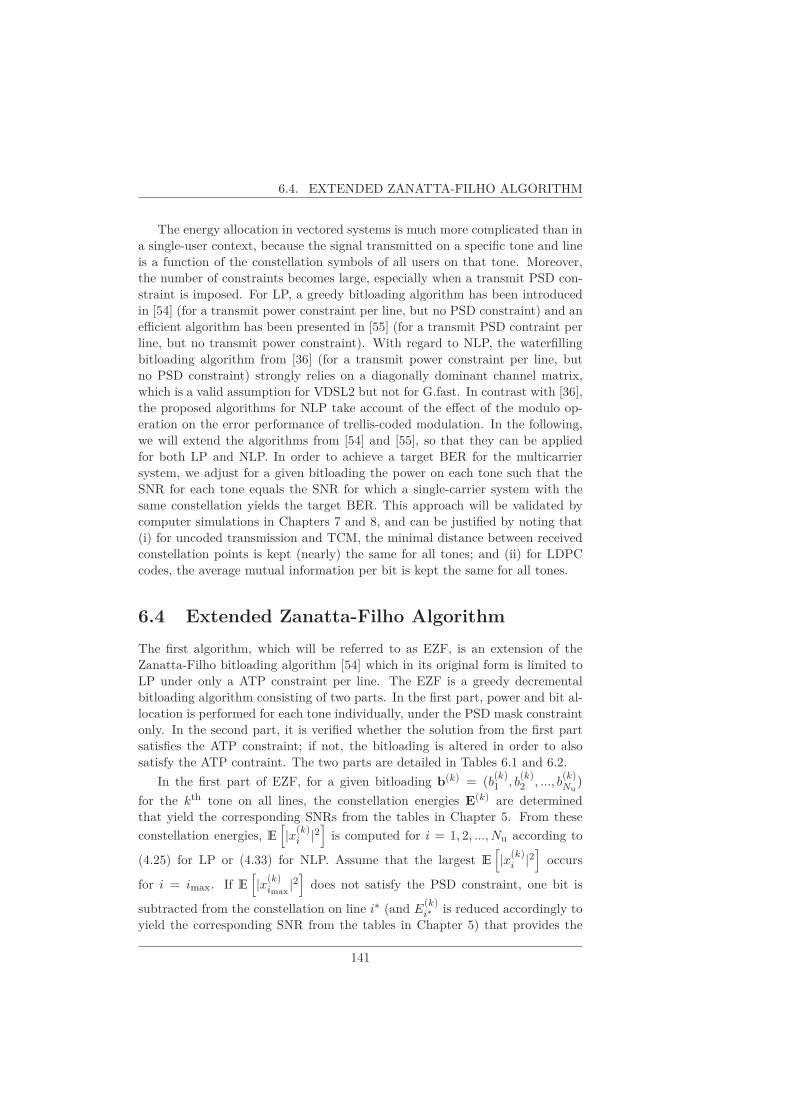
6.4. EXTENDED ZANATTA-FILHO ALGORITHM
The energy allocation in vectored systems is much more complicated than ina single-user context, because the signal transmitted on a specific tone and lineis a function of the constellation symbols of all users on that tone. Moreover,the number of constraints becomes large, especially when a transmit PSD con-straint is imposed. For LP, a greedy bitloading algorithm has been introducedin [54] (for a transmit power constraint per line, but no PSD constraint) and anefficient algorithm has been presented in [55] (for a transmit PSD contraint per
line, but no transmit power constraint). With regard to NLP, the waterfilling
bitloading algorithm from [36] (for a transmit power constraint per line, but
no PSD constraint) strongly relies on a diagonally dominant channel matrix,
which is a valid assumption for VDSL2 but not for G.fast. In contrast with [36],
the proposed algorithms for NLP take account of the effect of the modulo op-
eration on the error performance of trellis-coded modulation. In the following,
we will extend the algorithms from [54] and [55], so that they can be applied
for both LP and NLP. In order to achieve a target BER for the multicarrier
system, we adjust for a given bitloading the power on each tone such that the
SNR for each tone equals the SNR for which a single-carrier system with the
same constellation yields the target BER. This approach will be validated by
computer simulations in Chapters 7 and 8, and can be justified by noting that
(i) for uncoded transmission and TCM, the minimal distance between received
constellation points is kept (nearly) the same for all tones; and (ii) for LDPC
codes, the average mutual information per bit is kept the same for all tones.
6.4 Extended Zanatta-Filho Algorithm
The first algorithm, which will be referred to as EZF, is an extension of the
Zanatta-Filho bitloading algorithm [54] which in its original form is limited to
LP under only a ATP constraint per line. The EZF is a greedy decremental
bitloading algorithm consisting of two parts. In the first part, power and bit al-
location is performed for each tone individually, under the PSD mask constraint
only. In the second part, it is verified whether the solution from the first part
satisfies the ATP constraint; if not, the bitloading is altered in order to also
satisfy the ATP contraint. The two parts are detailed in Tables 6.1 and 6.2.
In the first part of EZF, for a given bitloading b(k) = (b(k)1 , b
(k)2 , ..., b
(k)Nu
)
for the kth tone on all lines, the constellation energies E(k) are determined
that yield the corresponding SNRs from the tables in Chapter 5. From these
constellation energies, E
[
|x(k)i |2
]
is computed for i = 1, 2, ...,Nu according to
(4.25) for LP or (4.33) for NLP. Assume that the largest E
[
|x(k)i |2
]
occurs
for i = imax. If E
[
|x(k)imax
|2]
does not satisfy the PSD constraint, one bit is
subtracted from the constellation on line i∗ (and E(k)i∗ is reduced accordingly to
yield the corresponding SNR from the tables in Chapter 5) that provides the
141

6. BITLOADING ALGORITHMS
Table 6.1: The EZF bit allocation algorithm.
PART I: Repeat for all tones k = 1, . . . ,Nt
1. Initialization: Set b(k)i = bmax ∀ lines i : 1 ≤ i ≤ Nu;
2. While ∃i : E[|x(k)
i |2]
> E(k)PSD:
(a) imax = argmaxi
(E
[|x(k)
i |2])
(b) For i = 1, . . . ,Nu : evaluate E[|x(k)
imax,i|2
], the energy transmitted on
line imax associated with decreasing 1 bit on tone k from line i ;
i. Let b(k)i = b
(k)i − 1;
ii. Evaluate the symbol energy E[|u(k)
i |2]on line i associated with
b(k)i ;
iii. Evaluate the transmitted energy E[|x(k)
imax,i|2
]at line imax, re-
quired for this new allocation on line i;
(c) Find i∗ such that i∗ = argminiE[|x(k)
imax,i|2
]
(d) Substract one bit at the optimum position: b(k)i∗ = b
(k)i∗ − 1;
(e) Compute E[|u(k)
i |2]and E
[|x(k)
i |2](for all i) for this new bit alloca-
tion;
3. End.
142

6.4. EXTENDED ZANATTA-FILHO ALGORITHM
Table 6.2: The EZF bit allocation algorithm.
PART II:While ∃i :∑Nt
k=1 E[|x(k)
i |2]
> EATP:
1. i′max = argmaxi
∑Ntk=1
(E
[|x(k)
i |2])
2. For i = 1, . . . ,Nu and k = 1, . . . ,Nt: evaluate E[|x(k)
i′max,i
|2], the energy
transmitted on line i′max associated with decreasing 1 bit on tone k from
line i ;
(a) Let b(k)i = b
(k)i − 1;
(b) Evaluate the symbol energy E(k)i on line i associated with bk
i ;
(c) Evaluate the transmitted energy at line i′max, E
[|x(k)
i′max,i
|2], required
for this new allocation on line i and tone k;
3. Find (i∗, k∗), such that (i∗, k∗) = argmaxi,kE[|x(k)
i′max
|2]
− E[|x(k)
i′max,i
|2]
4. Subtract one bit at the optimum position: b(k∗)i∗ = b
(k∗)i∗ − 1;
5. Compute E(k)i and E
[|x(k)
i |2](for k∗, all i) for this new bit allocation;
End.
143
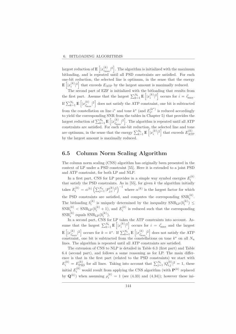
6. BITLOADING ALGORITHMS
largest reduction of E
[
|x(k)imax
|2]
. The algorithm is initialized with the maximum
bitloading, and is repeated until all PSD constraints are satisfied. For eachone-bit reduction, the selected line is optimum, in the sense that the energy
E
[
|x(k)i |2
]
that exceeds EATP by the largest amount is maximally reduced.
The second part of EZF is initialized with the bitloading that results from
the first part. Assume that the largest∑Nt
k=1 E
[
|x(k)i |2
]
occurs for i = i′max.
If∑Nt
k=1 E
[
|x(k)i′max
|2]
does not satisfy the ATP constraint, one bit is subtracted
from the constellation on line i∗ and tone k∗ (and E(k∗)i∗ is reduced accordingly
to yield the corresponding SNR from the tables in Chapter 5) that provides the
largest reduction of∑Nt
k=1 E
[
|x(k)i′max
|2]
. The algorithm is repeated until all ATP
constraints are satisfied. For each one-bit reduction, the selected line and tone
are optimum, in the sense that the energy∑Nt
k=1 E
[
|x(k)i |2
]
that exceeds E(k)ATP
by the largest amount is maximally reduced.
6.5 Column Norm Scaling Algorithm
The column norm scaling (CNS) algorithm has originally been presented in thecontext of LP under a PSD constraint [55]. Here it is extended to a joint PSDand ATP constraint, for both LP and NLP.
In a first part, CNS for LP provides in a simple way symbol energies E(k)i
that satisfy the PSD constraints. As in [55], for given k the algorithm initially
takes E(k)i = α(k)
(∑Nu
j=1 |P (k)j,i |2
)−1where α(k) is the largest factor for which
the PSD constraints are satisfied, and computes the corresponding SNR(k)i .
The bitloading b(k)i is uniquely determined by the inequality SNRLP(b
(k)i ) ≤
SNR(k)i < SNRLP(b
(k)i + 1), and E
(k)i is reduced such that the corresponding
SNR(k)i equals SNRLP(b
(k)i ).
In a second part, CNS for LP takes the ATP constraints into account. As-
sume that the largest∑Nt
k=1 E
[
|x(k)i |2
]
occurs for i = i′max and the largest
E
[
|x(k)i′max
|2]
occurs for k = k∗. If∑Nt
k=1 E
[
|x(k)i′max
|2]
does not satisfy the ATP
constraint, one bit is subtracted from the constellations on tone k∗ on all Nu
lines. The algorithm is repeated until all ATP constraints are satisfied.The extension of CNS to NLP is detailed in Table 6.3 (first part) and Table
6.4 (second part), and follows a same reasoning as for LP. The main differ-ence is that in the first part (related to the PSD constraints) we start with
E(k)i = E
(k)PSD for all lines. Taking into account that
∑Ntj=1 |Q(k)
i,j |2 = 1, these
initial E(k)i would result from applying the CNS algorithm (with P(k) replaced
by Q(k)) when assuming ρ(k)i = 1 (see (4.33) and (4.34)); however these ini-
144
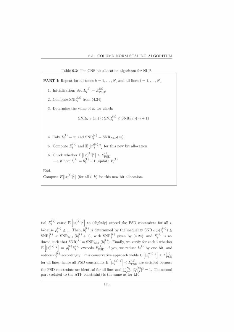
6.5. COLUMN NORM SCALING ALGORITHM
Table 6.3: The CNS bit allocation algorithm for NLP.
PART I: Repeat for all tones k = 1, . . . ,Nt and all lines i = 1, . . . ,Nu
1. Initialization: Set E(k)i = E
(k)PSD;
2. Compute SNR(k)i from (4.24)
3. Determine the value of m for which:
SNRNLP(m) < SNR(k)i ≤ SNRNLP(m + 1)
4. Take b(k)i = m and SNR
(k)i = SNRNLP(m);
5. Compute E(k)i and E
[|x′(k)
i |2]for this new bit allocation;
6. Check whether E[|x′(k)
i |2]
≤ E(k)PSD
−→ if not: b(k)i = b
(k)i − 1; update E
(k)i
End.
Compute E[|x(k)
i |2](for all i, k) for this new bit allocation.
tial E(k)i cause E
[
|x(k)i |2
]
to (slightly) exceed the PSD constraints for all i,
because ρ(k)i ≥ 1. Then, b
(k)i is determined by the inequality SNRNLP(b
(k)i ) ≤
SNR(k)i < SNRNLP(b
(k)i + 1), with SNR
(k)i given by (4.24), and E
(k)i is re-
duced such that SNR(k)i = SNRNLP(b
(k)i ). Finally, we verify for each i whether
E
[
|x′(k)i |2
]
= ρ(k)i E
(k)i exceeds E
(k)PSD; if yes, we reduce b
(k)i by one bit, and
reduce E(k)i accordingly. This conservative approach yields E
[
|x′(k)i |2
]
≤ E(k)PSD
for all lines; hence all PSD constraints E
[
|x(k)i |2
]
≤ E(k)PSD are satisfied because
the PSD constraints are identical for all lines and∑Nt
j=1 |Q(k)i,j |2 = 1. The second
part (related to the ATP constraint) is the same as for LP.
145

6. BITLOADING ALGORITHMS
Table 6.4: The CNS algorithm bit allocation algorithm for NLP.
PART II: While ∃i :∑Nt
k=1 E[|x(k)
i |2]
> EATP:
1. i′max = argmaxi
∑Ntk=1
(E
[|x(k)
i |2])
2. kmax = argmaxk E[|x(k)
i′max
|2]
3. For all lines, decrease the bitloading on tone kmax by 1 bit: b(kmax)i =
b(kmax)i − 1 for i = 1, 2, ...,Nu;
4. Compute E(k)i and E
[|x(k)
i |2](for kmax, all i) for this new bit allocation;
End.
6.6 EZF and CNS Complexity
In the first part of EZF, we start from the maximum bitloading, and reduce thebitloading by one bit at a time, until all PSD constraints are met. The first partrequires, per tone and per one-bit reduction, a search over Nu transmit ener-
gies E
[
|x(k)i |2
]
to determine imax, followed by the computation of and a search
over Nu transmit energies E
[
|x(k)imax
|2]
to determine i∗. In the second part of
EZF, we again reduce the bitloading by one bit at a time, until all ATP con-straints are satisfied. The second part requires, per one-bit reduction, a search
over Nu transmit energies∑Nt
k=1 E
[
|x(k)i |2
]
to determine i′max, followed by the
computation of and a search over NuNt transmit energies∑Nt
k=1 E
[
|x(k)i′max
|2]
to
determine (i∗, k∗).
In the first part of CNS, the constellation energies E(k)i and the correspond-
ing bitloadings b(k)i yielding transmit energies E
[
|x(k)i |2
]
that satisfy all PSD
constraints are computed directly, without requiring one-bit reduction nor anysearch. The second part of CNS involves reducing by one bit the bitloadings onall lines for a particular tone; this requires, per such reduction, a search over
Nu transmit energies∑Nt
k=1 E
[
|x(k)i |2
]
to determine i′max, followed by a search
over Nt transmit energies E
[
|x(k)i′max
|2]
to determine kmax.
The above considerations indicate that CNS has a much smaller computa-tional complexity, compared to EZF.
146
7Information Rates in the Ab-sence of Impulsive Noise
In this chapter, we apply the bit allocation algorithms from Chapter 6 to theDSL communication system described in Chapter 4. We compare the resultinginformation bitrates, goodput and computation times for the different precodingschemes in a G.fast downlink scenario without impulsive noise. We considerDSL loops of 100 m, 150 m, 200 m and 250 m and apply the different protectiontechniques that are described in Chapter 2. A binder consists of 8 paralleltwisted pair lines; the corresponding size-8x8 channel matrices for each tone havebeen obtained from measurements. The cable contains foam-skin polyethyleneinsulation and the copper diameter is 0.6 mm. Each line is assumed to beaffected by stationary white noise with PSD given by N0 = -140 dBm/Hz. TheG.fast-based DMT modulation uses frequencies up to 212 MHz, a tone spacingof 51.75 kHz and a DMT symbol rate of 48000 symbols/s. The transmissionpower PATP on each line is limited to 4 dBm. The maximum allowed BER isset to 10−7.
In Sections 7.1, 7.2, 7.3, 7.4 and 7.6 we consider respectively uncoded trans-
147

7. INFORMATION RATES IN THE ABSENCE OF IMPULSIVE NOISE
mission, TCM, LDPC codes, the concatenation of RS outer code + byte-interleaver+ TCM inner code, and ARQ.
7.1 Uncoded Transmission
In the case of uncoded transmission, the bit allocation algorithms make use ofTable 5.1 which contains the SNR levels for which the target BER of 10−7 isachieved for constellation sizes up to 212-QAM. After applying the bit allocationalgorithms on the different DSL loops, following results are obtained. For anarbitrary line (i = 4) in the 200 m DSL loop, the PSD mask, the transmit energy
E[|x(k)i |2], the constellation energy E
(k)i and the corresponding bitloading are
shown as a function of the tone frequency, in Figures 7.1, 7.2, 7.3 and 7.4, forseveral combinatons of precoding (LP or NLP) and bitloading (CNS of EZF):LP-CNS, NLP-CNS, LP-EZF and NLP-EZF, respectively. The results fromthese figures can be explained as follows:
• For tones at low frequencies (say, below 40 MHz), crosstalk is negligibleand the channel matrix can be considered diagonal. In this case, thetransmit energy and the constellation energy are essentially the same. ThePSD mask would allow constellation sizes exceeding 12 bit, but the numberof bits per constellation symbol is limited to 12: the transmit energy isadjusted such that BER = 10−7 for 212-QAM, and is substantially belowthe PSD mask.
• For tones in the medium frequency range (say, 40-120 MHz), the chan-nel matrix has significant off-diagonal elements, indicating the presence ofstrong crosstalk. For LP, the off-diagonal elements have a large impacton the constellation energies resulting from the bitloading, yielding strongfluctuations in constellation energy compared to the PSD mask. For NLP,this impact is much less, because of the modulo operation at the trans-mitter; in this case the constellation energy is much closer to the PSDmask.
• At high frequencies (say, above 120 MHz), several tones with zero bitload-ing occur, because of the very large signal attenuation. The correspond-
ing constellation energy E(k)i is obviously zero, but the transmit energy
E[|x(k)i |2] on these tones might be nonzero. This is because the transmit-
ted component x(k)i on line i depends on the constellation symbol energies
on all lines, according to the type of precoding used.
Table 7.1 compares the EZF and CNS bitloading algorithms in terms ofthe resulting average information bitrate per line, for LP and NLP and forthe different loop lengths. We observe that NLP outperforms LP by roughly
148

7.1. UNCODED TRANSMISSION
0 50 100 150 200
100
90
80
70
60
f!(MHz)
(dBm/Hz)
0 50 100 150 2000
2
4
6
8
10
12
f!(MHz)
PSD!mask
E4
(k)
E[|x4
(k)|2]
bit!loading
16934!bits/DMT!symbol
LP CNSline!4200!m!loop!length
Figure 7.1: PSD values and bitloading for line 4 of the 200 m loop with uncoded
transmission and LP-CNS.
149

7. INFORMATION RATES IN THE ABSENCE OF IMPULSIVE NOISE
0 50 100 150 200 100
95
90
85
80
75
70
65
f!(MHz)
(dBm/Hz)
0 50 100 150 2000
2
4
6
8
10
12
f!(MHz)
PSD!mask
E4
(k)
E[|x4
(k)|2]
bit!loading
17494!bits/DMT!symbol
NLP CNSline!4200!m!loop!length
Figure 7.2: PSD values and bitloading for line 4 of the 200 m loop with uncoded
transmission and NLP-CNS.
150

7.1. UNCODED TRANSMISSION
0 50 100 150 200 110
100
90
80
70
60
f!(MHz)
(dBm/Hz)
0 50 100 150 2000
2
4
6
8
10
12
f!(MHz)
PSD!mask
E4
(k)
E[|x4
(k)|2]
bit!loading
17597!bits/DMT!symbol
LP EZFline!4200!m!loop!length
Figure 7.3: PSD values and bitloading for line 4 of the 200 m loop with uncoded
transmission and LP-EZF.
151
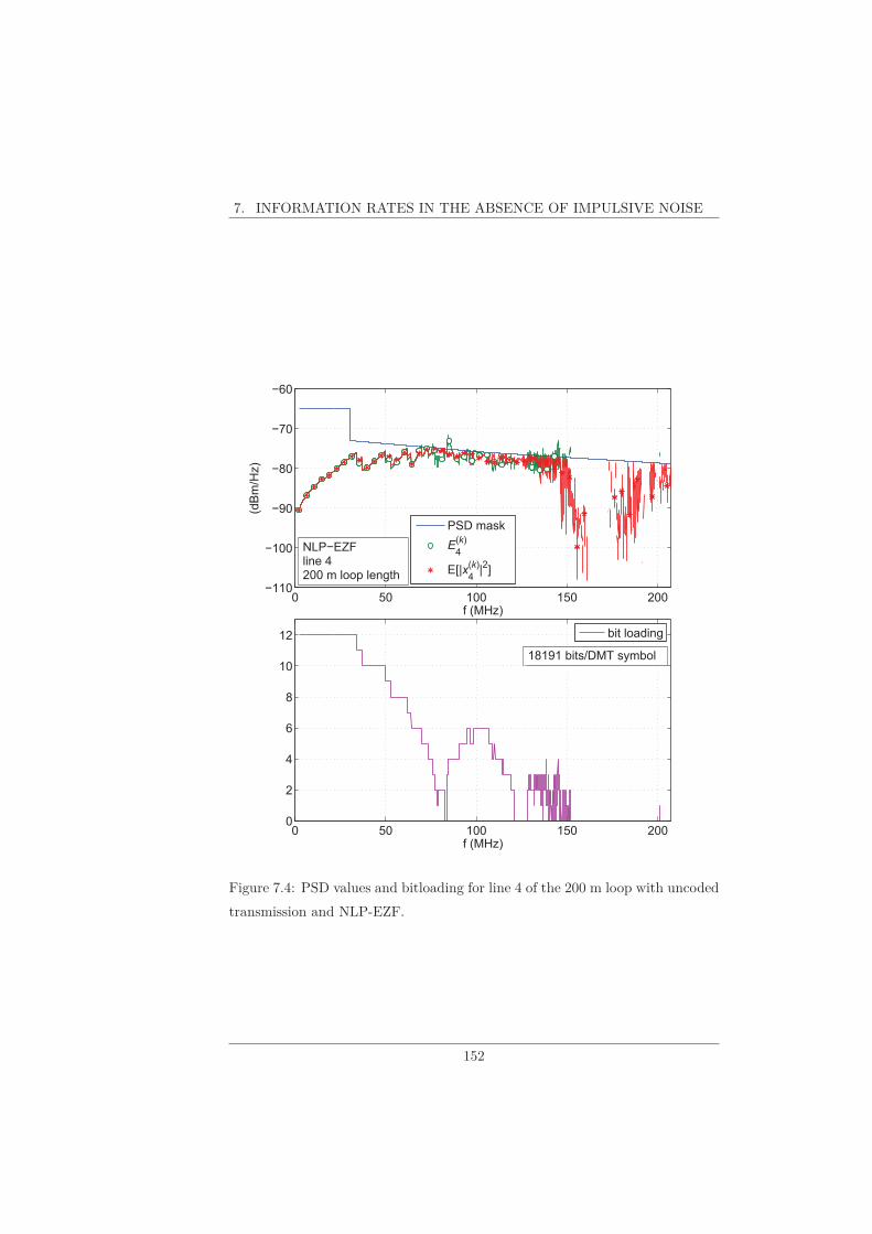
7. INFORMATION RATES IN THE ABSENCE OF IMPULSIVE NOISE
0 50 100 150 200 110
100
90
80
70
60
f!(MHz)
(dBm/Hz)
0 50 100 150 2000
2
4
6
8
10
12
f!(MHz)
bit!loading
PSD!mask
E4
(k)
E[|x4
(k)|2]
18191!bits/DMT!symbol
NLP EZFline!4200!m!loop!length
Figure 7.4: PSD values and bitloading for line 4 of the 200 m loop with uncoded
transmission and NLP-EZF.
152

7.2. TCM
Table 7.1: Average information bitrates (Gbps) per line for uncoded transmis-
sion.
100m 150m 200m 250m
LP-EZF 1.624 1.236 0.842 0.638
LP-CNS 1.575 1.213 0.817 0.615
NLP-EZF 1.764 1.339 0.930 0.695
NLP-CNS 1.741 1.325 0.919 0.688
Table 7.2: Computation time to determine the bitloading for uncoded transmis-
sion and all lines on all tones.
100m 150m 200m 250m
LP-EZF 3.06 s ⊗ 16.74 s ⊗ 13.52 s ⊗ 8.24 s ⊗LP-CNS 0.07 s 0.06 s 0.08 s 0.06 s
NLP-EZF 3.43 s ⊗ 22.75 s ⊗ 24.99 s ⊗ 16.01 s ⊗NLP-CNS 0.16 s 0.21 s ⊗ 0.19 s ⊗ 0.16 s
10% in terms of information rate. The differences between EZF and CNS areconsiderably less than 10%; EZF outperforms CNS by about 3% and 1.1% forLP and NLP, respectively.
Table 7.2 shows the computation times for the various combinations of pre-coding technique and bitloading algorithm, providing an indication of the rel-ative complexity of the algorithms; the symbol ⊗ indicates that part II of thealgorithm (related to the constraint on the transmission power per line) had tobe executed. We observe that CNS is at least a factor of 20 faster than EZF.Hence, the slightly higher information bitrate resulting from EZF compared toCNS comes at the cost of a considerably higher computational complexity.
7.2 TCM
In Chapter 5, Table 5.2 gives SNR values that are required for transmissionwith TCM to achieve exactly the target BER equal to 10−7. These SNR valuesare determined specifically for TCM codewords with a constant constellationsize on all tones in the DMT. To show that these table values are also valid for
153

7. INFORMATION RATES IN THE ABSENCE OF IMPULSIVE NOISE
10�7
10�6
10�5
10�4
10�3
10�2
10�8
10�6
10�4
10�2
100
target BER
BE
Ruser 1
user 2
user 3
user 4
user 5
user 6
user 7
user 8
100 m DSL loopNLP�EZF
Figure 7.5: Resulting BER versus target BER for TCM and the 100 m DSL
loop with 8 users.
TCM codewords with different constellation sizes on different tones in the DMT,simulations are performed on a real DSL loop, where we applied bitloadingfor target BER values ranging from 10−2 to 10−7; the SNR tables for targetBER values different from 10−7 were obtained in the same way as those forBER = 10−7. The actual BER resulting from the bitloading is shown in Figure7.5 versus the target BER, for the 100 m DSL loop with 8 lines and NLP-EZF.It is clear that there is a very good agreement between resulting BER and targetBER.
After applying the bit allocation algorithms from Chapter 6 on different DSLloops, following numerical results are obtained. For an arbitrary line (i = 4) in
the 200 m DSL loop, the PSD mask, the transmit energy E[|x(k)i |2], the con-
stellation energy E(k)i and the corresponding bitloading are shown as a function
of the tone frequency, in Figures 7.6, 7.7, 7.8 and 7.9, for LP-CNS, NLP-CNS,LP-EZF and NLP-ZF, respectively. A similar behaviour as with uncoded trans-mission is observed.
Table 7.3 compares the EZF and CNS bitloading algorithms in terms ofthe resulting average information bitrate per line, for LP and NLP and forthe different loop lengths. We observe that NLP outperforms LP by roughly10% in terms of information rate. The differences between EZF and CNS areconsiderably less; EZF outperforms CNS by about 3.7% and 1.3% for LP and
154
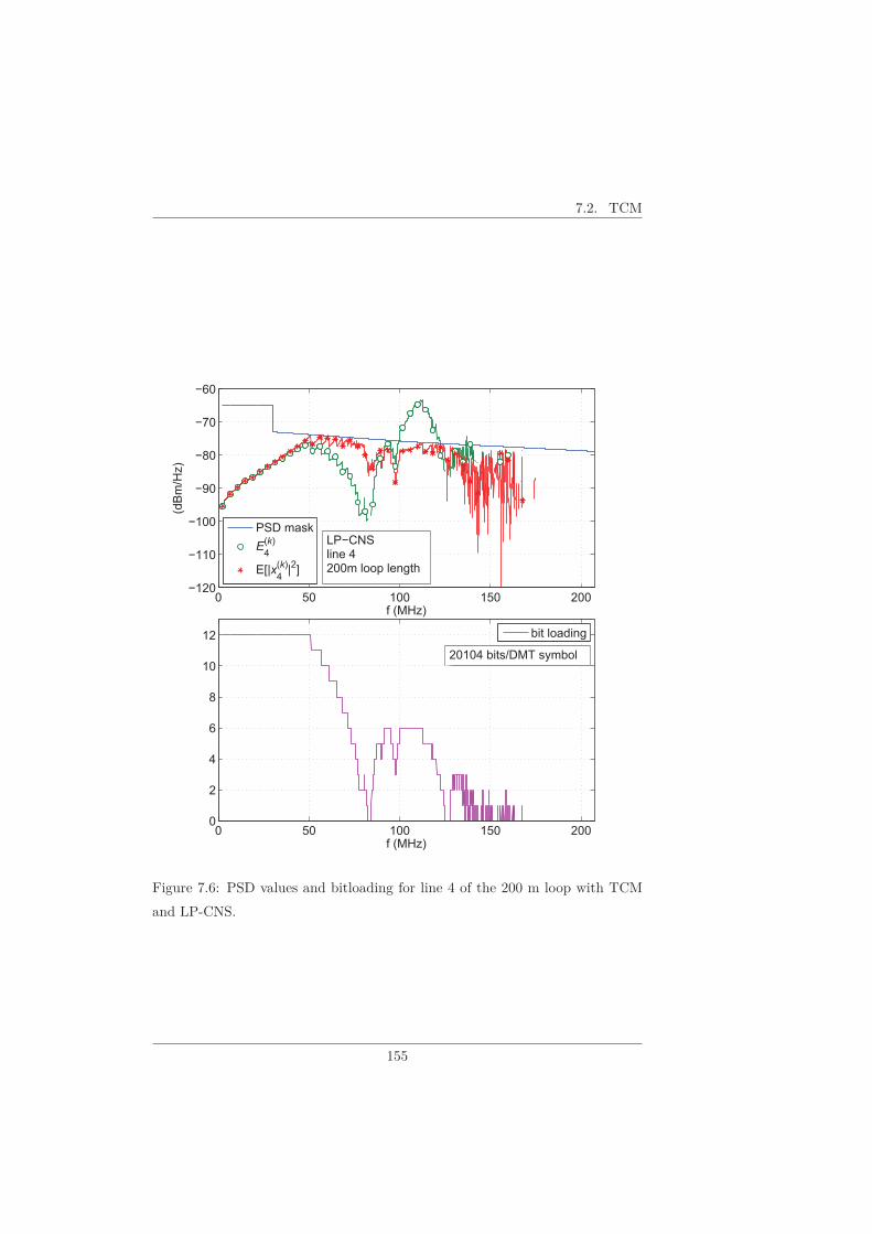
7.2. TCM
0 50 100 150 200 120
110
100
90
80
70
60
f!(MHz)
(dBm/Hz)
0 50 100 150 2000
2
4
6
8
10
12
f!(MHz)
bit!loading
PSD!mask
E4
(k)
E[|x4
(k)|2]
20104!bits/DMT!symbol
LP CNSline!4200m!loop!length
Figure 7.6: PSD values and bitloading for line 4 of the 200 m loop with TCM
and LP-CNS.
155

7. INFORMATION RATES IN THE ABSENCE OF IMPULSIVE NOISE
0 50 100 150 200 110
100
90
80
70
60
f!(MHz)
(dBm/Hz)
0 50 100 150 2000
2
4
6
8
10
12
f!(MHz)
bitloading
PSD!mask
E4
(k)
E[|x4
(k)|2]
21459!bits/DMT!symbol
NLP CNSline!4200m!loop!length
Figure 7.7: PSD values and bitloading for line 4 of the 200 m loop with TCM
and NLP-CNS.
156

7.2. TCM
0 50 100 150 200 120
110
100
90
80
70
60
f!(MHz)
(dBm/Hz)
0 50 100 150 2000
2
4
6
8
10
12
f!(MHz)
bit!loading
PSD!mask
E4
(k)
E[|x4
(k)|2]
20960!bits/DMT!symbol
LP EZFline!4200m!loop!length
Figure 7.8: PSD values and bitloading for line 4 of the 200 m loop with TCM
and LP-EZF.
157

7. INFORMATION RATES IN THE ABSENCE OF IMPULSIVE NOISE
0 50 100 150 200 120
110
100
90
80
70
60
f!(MHz)
(dBm/Hz)
0 50 100 150 2000
2
4
6
8
10
12
f!(MHz)
bit!loading
PSD!mask
E4
(k)
E[|x4
(k)|2]
22165!bits/DMT!symbol
NLP EZFline!4200m!loop!length
Figure 7.9: PSD values and bitloading for line 4 of the 200 m loop with TCM
and NLP-EZF.
158

7.3. LDPC CODES
Table 7.3: Average information bitrates (Gbps) per line for TCM.
100m 150m 200m 250m
LP-EZF 1.712 1.369 0.941 0.720
LP-CNS 1.665 1.324 0.904 0.690
NLP-EZF 1.846 1.482 1.055 0.786
NLP-CNS 1.825 1.460 1.040 0.775
Table 7.4: Computation time to determine the bitloading for TCM and all lines
on all tones.
100m 150m 200m 250m
LP-EZF 2.28 s 6.62 s ⊗ 8.88 s ⊗ 7.78 s ⊗LP-CNS 0.14 s 0.11 s 0.15 s 0.14 s
NLP-EZF 2.55 s 8.59 s ⊗ 20.91 s ⊗ 16.11 s ⊗NLP-CNS 0.21 s 0.22 s 0.36 s ⊗ 0.19 s
NLP, respectively.Table 7.4 shows the computation times for the various combinations of pre-
coding technique and bitloading algorithm; the symbol ⊗ again indicates thatpart II of the algorithm had to be executed. We observe that CNS is at least afactor of 10 faster than EZF. Similar as for uncoded transmission, the slightlyhigher information rate of TCM resulting from EZF compared to CNS comesat the cost of a considerably higher computational complexity.
7.3 LDPC Codes
In the case of LDPC coding, the bit allocation algorithms make use of tables,containing the SNR values for which the target BER is achieved for all QAMconstellations up to 212-QAM, for each code rate Rc and block length K; thesetables are similar to Table 5.11, which was specifically obtained for the LDPCcode with Rc = 20/21 and K = 4320. The required SNR values can be com-puted from the Iavg values given in Table 5.10. Although the LDPC codewordshave different constellation sizes on the different tones in the DMT symbol whentransmitting over the frequency-selective DSL channel, we have verified (in a
159

7. INFORMATION RATES IN THE ABSENCE OF IMPULSIVE NOISE
Table 7.5: Average information bitrates (Gbps) per line for all proposed LDPC
codes and loop length equal to 100 m.
100m Rc 1/2 2/3 5/6 16/18 20/21
K = 960
LP-EZF 1.080 1.361 1.604 1.653 1.698
LP-CNS 1.064 1.334 1.566 1.613 1.654
NLP-EZF 1.110 1.430 1.708 1.768 1.830
NLP-CNS 1.104 1.412 1.690 1.751 1.806
K = 4320
LP-EZF 1.096 1.387 1.637 1.702 1.757
LP-CNS 1.082 1.361 1.600 1.660 1.714
NLP-EZF 1.118 1.449 1.736 1.814 1.882
NLP-CNS 1.114 1.432 1.716 1.794 1.864
similar way as for TCM) that these SNR values remain valid to achieve theBER constraint; this is no surprise, because the error performance is essentiallydetermined by the Iavg value.
In this section, we show results pertaining to the SMSA decoder only, asit achieves the target BER at lower SNR values than the SPA decoder andfurthermore, it has a lower computation complexity.
Table 7.5 compares the EZF and CNS bitloading algorithm in terms of theaverage resulting information bitrate, for LP and NLP and a loop length of 100m; note that for a given code rate the longer codes yield the larger informationbitrate, because their better error performance allows to use larger constella-tions. In Table 7.6 we show results for CNS-NLP and the LDPC code for allrates and for K = 4320 only. We consider loop lengths of respectively 150 m,200 m and 250 m. We observe from Tables 7.5 and 7.6 that the more powerfullower-rate codes are outperformed in terms of information bitrate by the lesspowerful higher-rate codes. Compared to higher-rate codes, the lower-rate codesallow to use larger constellations for given SNR, but these larger constellationscontain a smaller fraction of information bits; the latter effect turns out to bedominant so that the information rate increases with the code rate. This can beexplained by noting that many tones (at low and medium frequencies) operateat high SNR, in which case that the higher code rates are more advantageousin terms of information bitrate (see discussion regarding Figure 6.3).
160
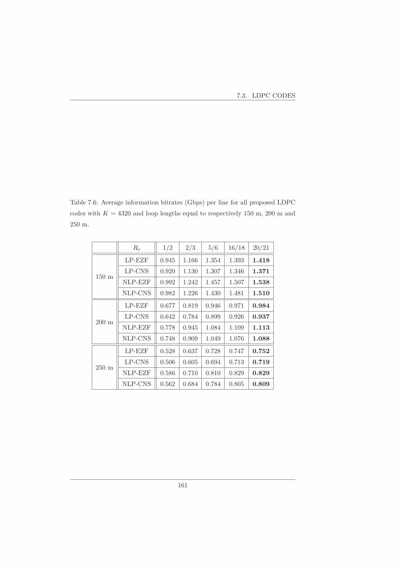
7.3. LDPC CODES
Table 7.6: Average information bitrates (Gbps) per line for all proposed LDPC
codes with K = 4320 and loop lengths equal to respectively 150 m, 200 m and
250 m.
Rc 1/2 2/3 5/6 16/18 20/21
150 m
LP-EZF 0.945 1.166 1.354 1.393 1.418
LP-CNS 0.920 1.130 1.307 1.346 1.371
NLP-EZF 0.992 1.242 1.457 1.507 1.538
NLP-CNS 0.982 1.226 1.430 1.481 1.510
200 m
LP-EZF 0.677 0.819 0.946 0.971 0.984
LP-CNS 0.642 0.784 0.899 0.926 0.937
NLP-EZF 0.778 0.945 1.084 1.109 1.113
NLP-CNS 0.748 0.909 1.049 1.076 1.088
250 m
LP-EZF 0.528 0.637 0.728 0.747 0.752
LP-CNS 0.506 0.605 0.694 0.713 0.719
NLP-EZF 0.586 0.710 0.810 0.829 0.829
NLP-CNS 0.562 0.684 0.784 0.805 0.809
161

7. INFORMATION RATES IN THE ABSENCE OF IMPULSIVE NOISE
Table 7.7: Average information bitrates (Gbps) per line for RS(255,236) + byte-
interleaver + TCM.
100m 150m 200m 250m
LP-EZF 1.681 1.372 0.958 0.735
LP-CNS 1.641 1.325 0.916 0.703
NLP-EZF 1.795 1.481 1.079 0.806
NLP-CNS 1.776 1.456 1.058 0.790
Table 7.8: Average information bitrates (Gbps) per line for RS(136,120) + byte-
interleaver + TCM .
100m 150m 200m 250m
LP-EZF 1.588 1.298 0.907 0.697
LP-CNS 1.550 1.253 0.867 0.666
NLP-EZF 1.695 1.400 1.022 0.763
NLP-CNS 1.676 1.337 1.003 0.748
7.4 RS + Byte-Interleaver + TCM
In Section 5.5.2, we analyzed the concatenation of RS and TCM assuming aconstant constellation size and constant SNR on all tones, for two RS codes:RS(255,239) and RS(136,120). Here we apply the bitloading, using the resultingSNR Table 5.12, for the different DSL loops at our disposal. Figure 7.10 com-
pares the PSD mask with the transmit energy E[|x(k)i |2] and the constellation
energy E(k)i for RS(255,236) + byte-interleaver + TCM and LP with the EZF
algorithm, along with the corresponding bitloading, for an arbitrary line (i = 4)in the 200 m DSL loop. As the concatenated coding scheme is more powerfulthan TCM, we can transmit larger constellation symbols, compared to Figure7.8. This results in a large number of coded bits per DMT symbol.
The resulting average information bitrates per line are given in Tables 7.7 and7.8 for the concatenated codes with respectively RS(255,239) and RS(136,120).
162
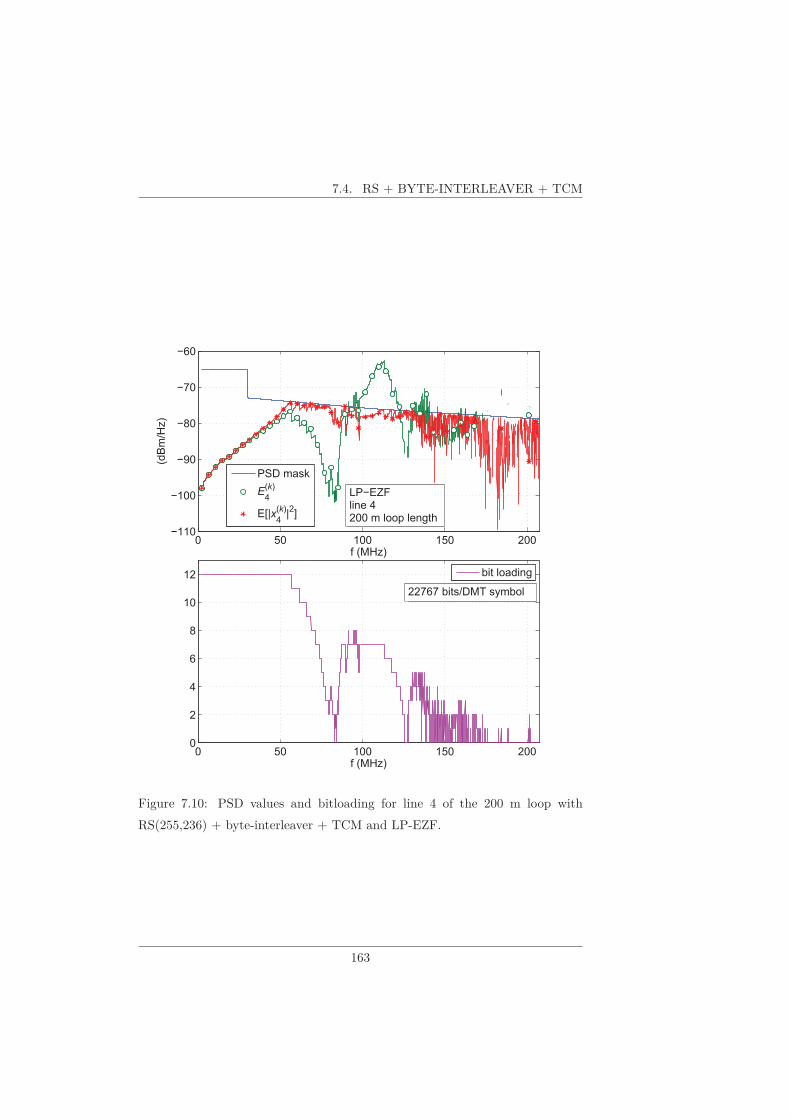
7.4. RS + BYTE-INTERLEAVER + TCM
0 50 100 150 200 110
100
90
80
70
60
f!(MHz)
(dBm/Hz)
0 50 100 150 2000
2
4
6
8
10
12
f!(MHz)
PSD!mask
E4
(k)
E[|x4
(k)|2]
bit!loading
22767!bits/DMT!symbol
LP EZFline!4200!m!loop!length
Figure 7.10: PSD values and bitloading for line 4 of the 200 m loop with
RS(255,236) + byte-interleaver + TCM and LP-EZF.
163

7. INFORMATION RATES IN THE ABSENCE OF IMPULSIVE NOISE
100 150 200 250
0.8
1
1.2
1.4
1.6
1.8
2
loop length (m)
info
rmation b
itra
te (
Gbps)
uncoded
TCM
RS(255,239)+intrlvr+TCM
RS(136,120)+intrlvr+TCM
LDPC, Rc = 20/21, K = 4320
Figure 7.11: Comparison of the average information bitrate versus loop length
for EZF-NLP and several protection strategies.
7.5 Comparison
Figure 7.11 shows the average information bitrates versus the loop length forall protection strategies considered so far in this chapter, assuming NLP-EZF.In order not to overload the figure, the results for the LDPC codes are limitedto the LDPC code of rate 20/21 and K = 4320, as it achieves the largestinformation bitrates from Tables 7.5-7.6.
This comparison points out that the rate 20/21 LDPC code outperforms theother protection strategies for all loop lengths. Depending on the loop length, ei-ther TCM or RS(255,239) + byte-interleaver + TCM provide the second largestinformation bitrates; the former is better for the larger loop lengths, which op-erate at lower SNR. The RS(136,120) + byte-interleaver + TCM concatenationperforms worse in terms of information bitrate due to the larger encoding over-head compared to RS(255,239) + byte-interleaver + TCM. Uncoded transmis-sion achieves the lowest information bitrate for 150 m, 200 m and 250 m looplengths, whereas for a 100 m loop the RS(136,120) + byte-interleaver + TCMconcatenation yields the smallest information bitrate. These conclusions alsohold for the other combinations of precoder and bitloading algorithms.
164

7.6. ARQ
7.6 ARQ
In this section, we add ARQ on top of the protection strategies from the previoussections, except for the concatenation of RS and TCM, because the use of theRS outer code is already considered as an additional protection of TCM.
When using ARQ, the residual BER after Nretr retransmissions can be re-duced by increasing Nretr (at the expense of increased latency). Hence, under aBER constraint, the number of information bits per DMT symbol increases withNretr. However, as some of the DMT symbols also contain retransmitted data,we consider the goodput (see Section 2.8) as the proper performance indicator.Therefore, we will adopt the following approach in the case of ARQ:
1. We apply the bitloading using the SNR tables associated with a targetvalue of the BER in the absence of ARQ, denoted BER(0). From theobtained bitloading, we determine for each line the corresponding WERin the absence of ARQ, along with the associated goodput, denoted re-
spectively WER(0)i and GPi for line i; we have GPi = Rb,i(1−WER
(0)i ),
where Rb,i is the information bitrate on line i. We compute the averagegoodput over all lines, denoted GP. This is repeated for several values ofthe BER target value, which yields GP as a function of BER(0).
2. We determine the value BER(0)opt of BER
(0), such that GP achieves its
maximum value GPopt. The corresponding WER for line i is denoted
WER(0)opt,i.
3. Using the expression BER(Nretr)opt,i = BER
(0)opt
(
WER(0)opt,i
)Nretr
for the resid-
ual BER on line i when allowing Nretr retransmissions, we compute the
average residual BER over all lines, denoted BER(Nretr)opt , as a function of
Nretr. We determine the smallest value of Nretr (denoted Nretr,opt) which
yields BER(Nretr)opt ≤ 10−7.
4. The system will be operated using the bitloading corresponding to BER(0) =
BER(0)opt, and using ARQ allowing Nretr = Nretr,opt retransmissions. This
way, the resulting average goodput equals the maximum value GPopt, andthe residual BER after Nretr,opt retransmissions does not exceed 10−7. Of
course, one can achieve GP = GPopt with BER(Nretr)opt ≤ 10−7 for any
Nretr ≥ Nretr,opt, but selecting Nretr = Nretr,opt yields the maximum av-erage output with minimum latency.
The word error rateWER(0)i (or a close approximation thereof) has been deter-
mined from the symbol error probability in the case of uncoded transmission,from the trellis section error probability in the case of TCM, from the averagemutual information per bit Iavg in the case of LDPC codes, and from the TCMbyte error rate in the case of the concatenation of RS and TCM.
165
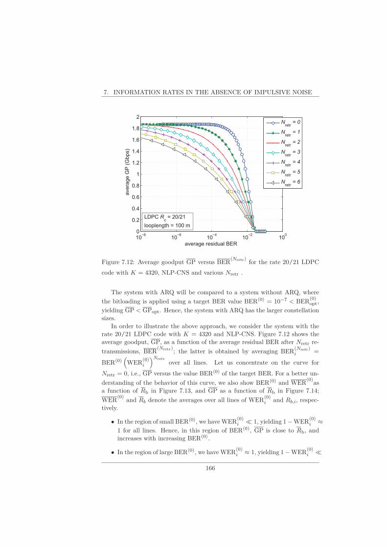
7. INFORMATION RATES IN THE ABSENCE OF IMPULSIVE NOISE
10�8
10�6
10�4
10�2
100
0
0.2
0.4
0.6
0.8
1
1.2
1.4
1.6
1.8
2
avera
ge G
P (
Gbps)
average residual BER
Nretr
= 0
Nretr
= 1
Nretr
= 2
Nretr
= 3
Nretr
= 4
Nretr
= 5
Nretr
= 6
LDPC Rc = 20/21
looplength = 100 m
Figure 7.12: Average goodput GP versus BER(Nretr) for the rate 20/21 LDPC
code with K = 4320, NLP-CNS and various Nretr .
The system with ARQ will be compared to a system without ARQ, where
the bitloading is applied using a target BER value BER(0) = 10−7 < BER(0)opt,
yielding GP < GPopt. Hence, the system with ARQ has the larger constellationsizes.
In order to illustrate the above approach, we consider the system with therate 20/21 LDPC code with K = 4320 and NLP-CNS. Figure 7.12 shows theaverage goodput, GP, as a function of the average residual BER after Nretr re-
transmissions, BER(Nretr); the latter is obtained by averaging BER
(Nretr)i =
BER(0)(
WER(0)i
)Nretr
over all lines. Let us concentrate on the curve for
Nretr = 0, i.e., GP versus the value BER(0) of the target BER. For a better un-
derstanding of the behavior of this curve, we also show BER(0) and WER(0)as
a function of Rb in Figure 7.13, and GP as a function of Rb in Figure 7.14;
WER(0)
and Rb denote the averages over all lines of WER(0)i and Rb,i, respec-
tively.
• In the region of small BER(0), we haveWER(0)i ≪ 1, yielding 1−WER
(0)i ≈
1 for all lines. Hence, in this region of BER(0), GP is close to Rb, andincreases with increasing BER(0).
• In the region of large BER(0), we haveWER(0)i ≈ 1, yielding 1−WER
(0)i ≪
166

7.6. ARQ
1.85 1.9 1.95 210
8
10 6
10 4
10 2
100
average Rb!(Gbps)
average!WER,!no!IN
average!BER,!no!IN
LDPC Rc!=!20/21
loop!length!=!100!m
Figure 7.13: WER(0)
and BER(0) versus Rb for the rate 20/21 LDPC code with
K = 4320, NLP-CNS and Nretr = 0.
1. Hence, GP is much smaller than Rb. Increasing BER(0) yields an in-
crease of Rb but a decrease of 1−WER(0)i . The latter effect is dominant
in the considered region of BER(0), hence GP decreases with increasingBER(0).
• In between, GP achieves a maximum value GPopt at BER(0) = BER(0)opt.
For Nretr > 1, the maximum goodput value GPopt occurs at BER(Nretr) =
BER(Nretr)opt , which implies that the abscissa of the maximum goodput value
shifts to the left with increasing Nretr. For the case at hand, we have BER(0)opt =
1.3 · 10−5 and BER(1)opt = 1.3 · 10−8, so that Nretr,opt = 1.
Tables 7.9-7.12 show for the different protection strategies the maximumaverage goodput under the error performance constraint BER ≤ 10−7 for thecases with ARQ and without ARQ. For uncoded transmission and TCM, theinformation word consists of 4320 bits and the LDPC codes have K = 4320
information bits; for the concatenation of the RS outer code, the infinite byteinterleaver and TCM, only the traditional RS(255, 239) code is considered. Inthe case of ARQ, the value of Nretr,opt is indicated between parentheses . Thefollowing observations can be made:
• In the case of ARQ, we achieve GP = GPopt for Nretr,opt = 1. The latency
167
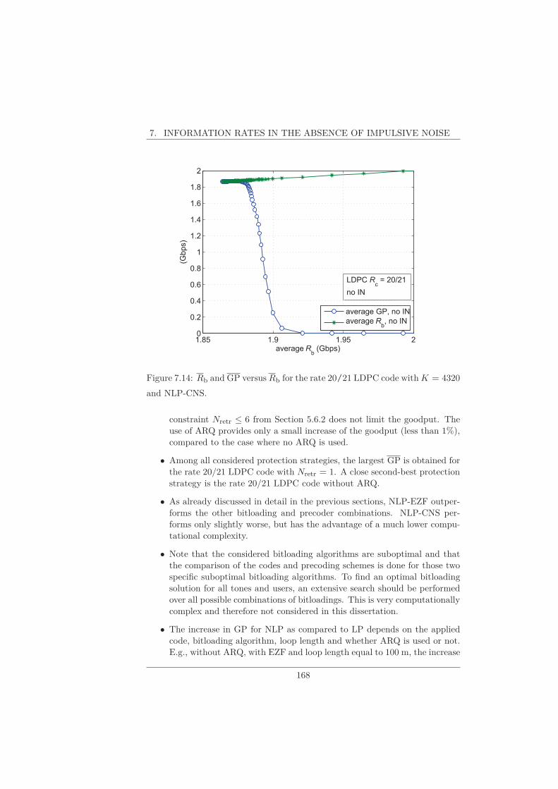
7. INFORMATION RATES IN THE ABSENCE OF IMPULSIVE NOISE
1.85 1.9 1.95 20
0.2
0.4
0.6
0.8
1
1.2
1.4
1.6
1.8
2
average Rb (Gbps)
(Gbps)
average GP, no IN
average Rb, no IN
LDPC Rc = 20/21
no IN
Figure 7.14: Rb andGP versus Rb for the rate 20/21 LDPC code with K = 4320
and NLP-CNS.
constraint Nretr ≤ 6 from Section 5.6.2 does not limit the goodput. Theuse of ARQ provides only a small increase of the goodput (less than 1%),compared to the case where no ARQ is used.
• Among all considered protection strategies, the largest GP is obtained forthe rate 20/21 LDPC code with Nretr = 1. A close second-best protectionstrategy is the rate 20/21 LDPC code without ARQ.
• As already discussed in detail in the previous sections, NLP-EZF outper-forms the other bitloading and precoder combinations. NLP-CNS per-forms only slightly worse, but has the advantage of a much lower compu-tational complexity.
• Note that the considered bitloading algorithms are suboptimal and thatthe comparison of the codes and precoding schemes is done for those twospecific suboptimal bitloading algorithms. To find an optimal bitloadingsolution for all tones and users, an extensive search should be performedover all possible combinations of bitloadings. This is very computationallycomplex and therefore not considered in this dissertation.
• The increase in GP for NLP as compared to LP depends on the appliedcode, bitloading algorithm, loop length and whether ARQ is used or not.E.g., without ARQ, with EZF and loop length equal to 100 m, the increase
168

7.6. ARQ
Table 7.9: Average goodput (Gbps) per line for BER ≤ 10−7 for 100 m loop
length.
LP-EZF LP-CNS NLP-EZF NLP-CNS
uncoded, no ARQ 1.616 1.567 1.755 1.733
uncoded, ARQ 1.645 (1) 1.598 (1) 1.783 (1) 1.760 (1)
TCM, no ARQ 1.704 1.657 1.838 1.818
TCM, ARQ 1.731 (1) 1.684 (1) 1.860 (1) 1.841 (1)
LDPC 1/2, no ARQ 1.095 1.081 1.118 1.114
LDPC 1/2, ARQ 1.098 (1) 1.084 (1) 1.118 (1) 1.115 (1)
LDPC 2/3, no ARQ 1.387 1.361 1.449 1.432
LDPC 2/3, ARQ 1.393 (1) 1.367 (1) 1.452 (1) 1.435 (1)
LDPC 5/6, no ARQ 1.637 1.600 1.736 1.716
LDPC 5/6, ARQ 1.644 (1) 1.608 (1) 1.743 (1) 1.722 (1)
LDPC 16/18, no ARQ 1.702 1.660 1.814 1.794
LDPC 16/18, ARQ 1.710 (1) 1.670 (1) 1.820 (1) 1.802 (1)
LDPC 20/21, no ARQ 1.757 1.714 1.882 1.864
LDPC 20/21, ARQ 1.766 (1) 1.723 (1) 1.889 (1) 1.872 (1)
RS(255,239)+TCM, no ARQ 1.681 1.641 1.795 1.776
ranges from 2.1% for the LDPC code of rate 1/2 and K = 4320 up to8.6% for uncoded transmission. The codes with the smaller code rate havethe smaller advantage of using NLP over LP.
• The increase in GP for EZF as compared to CNS depends on the appliedcode, precoding scheme, loop length and whether ARQ is used or not.E.g., without ARQ, with LP and loop length equal to 100 m, the increaseranges from 1.3% for LDPC code of rate 1/2 and K = 4320 up to 3%for uncoded transmission. The codes with the smaller code rate have thesmaller advantage of using EZF over CNS.
169

7. INFORMATION RATES IN THE ABSENCE OF IMPULSIVE NOISE
Table 7.10: Average goodput (Gbps) per line for BER ≤ 10−7 for 150 m loop
length.
LP-EZF LP-CNS NLP-EZF NLP-CNS
uncoded, no ARQ 1.231 1.207 1.332 1.319
uncoded, ARQ 1.270 (1) 1.239 (1) 1.376 (1) 1.353 (1)
TCM, no ARQ 1.345 1.317 1.477 1.455
TCM, ARQ 1.377 (1) 1.350 (1) 1.511 (1) 1.486 (1)
LDPC 1/2, no ARQ 0.945 0.919 0.992 0.982
LDPC 1/2, ARQ 0.949 (1) 0.924 (1) 0.995 (1) 0.985 (1)
LDPC 2/3, no ARQ 1.166 1.130 1.249 1.226
LDPC 2/3, ARQ 1.273 (1) 1.137 (1) 1.248 (1) 1.232 (1)
LDPC 5/6, no ARQ 1.354 1.307 1.457 1.430
LDPC 5/6, ARQ 1.363 (1) 1.316 (1) 1.465 (1) 1.439 (1)
LDPC 16/18, no ARQ 1.393 1.346 1.507 1.481
LDPC 16/18, ARQ 1.402 (1) 1.355 (1) 1.515 (1) 1.488 (1)
LDPC 20/21, no ARQ 1.418 1.371 1.538 1.509
LDPC 20/21, ARQ 1.430 (1) 1.381 (1) 1.549 (1) 1.521 (1)
RS(255,239)+TCM, no ARQ 1.372 1.352 1.481 1.456
170

7.6. ARQ
Table 7.11: Average goodput (Gbps) per line for BER ≤ 10−7 for 200 m loop
length.
LP-EZF LP-CNS NLP-EZF NLP-CNS
uncoded, no ARQ 0.838 0.813 0.926 0.915
uncoded, ARQ 0.867 (1) 0.839 (1) 0.962 (1) 0.945 (1)
TCM, no ARQ 0.937 0.900 1.051 1.036
TCM, ARQ 0.968 (1) 0.924 (1) 1.087 (1) 1.068 (1)
LDPC 1/2, no ARQ 0.677 0.642 0.778 0.746
LDPC 1/2, ARQ 0.682 (1) 0.647 (1) 0.781 (1) 0.750 (1)
LDPC 2/3, no ARQ 0.819 0.784 0.945 0.909
LDPC 2/3, ARQ 0.825 (1) 0.780 (1) 0.951 (1) 0.916 (1)
LDPC 5/6, no ARQ 0.946 0.899 1.084 1.049
LDPC 5/6, ARQ 0.952 (1) 0.906 (1) 1.093 (1) 1.058 (1)
LDPC 16/18, no ARQ 0.971 0.926 1.109 1.076
LDPC 16/18, ARQ 0.979 (1) 0.932 (1) 1.118 (1) 1.084 (1)
LDPC 20/21, no ARQ 0.984 0.936 1.112 1.088
LDPC 20/21, ARQ 0.993 (1) 0.944 (1) 1.124 (1) 1.097 (1)
RS(255,239)+TCM, no ARQ 0.958 0.916 1.079 1.058
171

7. INFORMATION RATES IN THE ABSENCE OF IMPULSIVE NOISE
Table 7.12: Average goodput (Gbps) per line for BER ≤ 10−7 for 250 m loop
length.
LP-EZF LP-CNS NLP-EZF NLP-CNS
uncoded, no ARQ 0.635 0.613 0.692 0.685
uncoded, ARQ 0.658 (1) 0.633 (1) 0.717 (1) 0.703 (1)
TCM, no ARQ 0.717 0.687 0.783 0.778
TCM, ARQ 0.740 (1) 0.710 (1) 0.810 (1) 0.798 (1)
LDPC 1/2, no ARQ 0.528 0.503 0.586 0.562
LDPC 1/2, ARQ 0.531 (1) 0.506 (1) 0.589 (1) 0.566 (1)
LDPC 2/3, no ARQ 0.637 0.605 0.710 0.684
LDPC 2/3, ARQ 0.641 (1) 0.610 (1) 0.715 (1) 0.689 (1)
LDPC 5/6, no ARQ 0.728 0.694 0.810 0.784
LDPC 5/6, ARQ 0.734 (1) 0.700 (1) 0.817 (1) 0.790 (1)
LDPC 16/18, no ARQ 0.747 0.713 0.829 0.805
LDPC 16/18, ARQ 0.753 (1) 0.718 (1) 0.835 (1) 0.811 (1)
LDPC 20/21, no ARQ 0.752 0.719 0.829 0.809
LDPC 20/21, ARQ 0.759 (1) 0.725 (1) 0.838 (1) 0.818 (1)
RS(255,239)+TCM, no ARQ 0.735 0.703 0.806 0.790
172

8Information Rates in the Pres-ence of Impulsive Noise
In this chapter, we apply the bit allocation algorithms from Chapter 6 to theDSL channel as described in Chapter 4; we use the same DSL loops as describedin Chapter 7, additionally here we assume the presence of IN on the channel.
We compare the resulting information bitrates and goodput for the differentprecoding schemes and bit allocation algorithms in a G.fast downlink scenariowith impulsive noise for different protection techniques. For each protectiontechnique considered, we distinguish between two cases. First, we assume thatthe parameters (p1,κ) of the impulsive noise model are known. In the secondcase, we have no information about the impulsive noise model.
In Sections 8.1, 8.2, 8.3, and 8.4 we consider respectively uncoded trans-mission, TCM, LDPC codes, and the concatenation of RS outer code + byte-interleaver + TCM inner code, all in the case where the parameters of the INmodel are known. A comparison of the achieved information bitrates is pre-sented in Section 8.5. Section 8.6 deals with the case where the parameters ofthe IN model are unknown. The use of ARQ is investigated in Section 8.7.
173

8. INFORMATION RATES IN THE PRESENCE OF IMPULSIVE NOISE
Table 8.1: Average information bitrates (Gbps) per line for uncoded transmis-
sion and IN with κ = 10 dB.
100m 150m 200m 250m
LP-EZF 1.173 0.848 0.587 0.447
LP-CNS 1.031 0.739 0.516 0.402
NLP-EZF 1.281 0.912 0.626 0.471
NLP-CNS 1.271 0.889 0.616 0.462
8.1 Uncoded Transmission
In the case of uncoded transmission and under the assumption that the pa-rameters of the IN model are known, the bit allocation algorithms make useof Tables 5.6 and 5.7 which contain the values of SNRavg for which the BER(averaged over the DMT symbols with and without IN) equals the target BERof 10−7, for constellation sizes up to 212-QAM and respectively κ = 10 dB andκ = 20 dB. After applying the bit allocation algorithms on the different DSLloops, the following results are obtained. Figures 8.1 and 8.2 show the PSD
mask, the transmit energy E[|x(k)i |2] and the constellation energy E
(k)i for un-
coded transmission with NLP-CNS and respectively κ = 10 dB and κ = 20 dB,along with the corresponding bitloading, for an arbitrary line (i = 4) in the200 m DSL loop. Notice that for an increasing level of IN fewer tones are used,more specifically only the lower-frequency tones remain active. It is clear thatIN has a large impact on the obtainable information bitrate. Tables 8.1 and8.2 compare the resulting information bitrates for all combinations of precod-ing types and bitloading algorithms. We observe that NLP outperforms LP byabout 22% and 5.6% for CNS and EZF, respectively. Regarding the differencebetween EZF and CNS, EZF outperforms CNS by about 18% and 2.4% for LPand NLP, respectively.
8.2 TCM
For TCM, similar computations are performed as for uncoded transmission inthe presence of IN and the results are presented in this section. Tables 5.8 and5.9 give the values of SNRavg that are required to achieve exactly the target BERequal to 10−7 for respectively κ = 10 dB and κ = 20 dB. These SNR valuesare determined specifically for TCM codewords with a constant constellationsize on all tones in the DMT. To show that these table values are also valid for
174

8.2. TCM
0 50 100 150 200 100
95
90
85
80
75
70
65
f!(MHz)
(dBm/Hz)
0 50 100 150 2000
2
4
6
8
10
12
f!(MHz)
PSD!mask
E4
(k)
E[|x4
(k)|2]
bit!loading
11681!bits/DMT!symbol
NLP CNSline!4200!m!loop!length
κ!=!10!dB
Figure 8.1: PSD values and bitloading for line 4 of the 200 m loop with κ = 10
dB, uncoded transmission and NLP-CNS.
175

8. INFORMATION RATES IN THE PRESENCE OF IMPULSIVE NOISE
0 50 100 150 200 100
95
90
85
80
75
70
65
f!(MHz)
(dBm/Hz)
0 50 100 150 2000
2
4
6
8
10
12
f!(MHz)
bit!loading
PSD!mask
E4
(k)
E[|x4
(k)|2]
7097!bits/DMT!symbol
NLP CNSline!4200!m!loop!length
κ = 20 dB
Figure 8.2: PSD values and bitloading for line 4 of the 200 m loop with κ = 20
dB, uncoded transmission and NLP-CNS.
176

8.2. TCM
Table 8.2: Average information bitrates (Gbps) per line for uncoded transmis-
sion and IN with κ = 20 dB.
100m 150m 200m 250m
LP-EZF 0.734 0.515 0.374 0.276
LP-CNS 0.590 0.414 0.306 0.231
NLP-EZF 0.789 0.544 0.380 0.280
NLP-CNS 0.777 0.515 0.372 0.271
Table 8.3: Average information bitrates (Gbps) per line for TCM and IN with
κ = 10 dB.
100m 150m 200m 250m
LP-EZF 1.336 0.980 0.668 0.510
LP-CNS 1.323 0.843 0.663 0.435
NLP-EZF 1.455 1.053 0.717 0.543
NLP-CNS 1.440 1.038 0.705 0.534
TCM codewords with different constellation sizes on different tones in the DMT,simulations are performed on a real DSL loop for target BER values rangingfrom 10−2 to 10−7. Similarly as for 10−7, we obtained tables with SNR valuesfor the other target BER values. The resulting BER is shown in Figure 8.3versus the target BER for the 100 m DSL loop with 8 lines, IN with κ = 10 dBand NLP-EZF. It is clear that there is a good correspondence between resultingBER and target BER. Also for TCM, IN has a large impact on the obtainableinformation rates. Tables 8.3 and 8.4 show the resulting average informationbitrate for EZF and CNS, for LP and NLP and for respectively κ = 10 dB andκ = 20 dB. We observe that the combination NLP-EZF achieves the highestbitrate, but only slightly better than NLP-CNS at the cost of a considerablyhigher computational complexity. Compared to NLP-CNS, NLP-EZF yields aninformation rate which is only 1.4% and 3.5% larger, for κ = 10 dB and κ = 20
dB, respectively.
177

8. INFORMATION RATES IN THE PRESENCE OF IMPULSIVE NOISE
10�7
10�6
10�5
10�4
10�3
10�2
10�8
10�6
10�4
10�2
100
target BER
BE
R
user 1
user 2
user 3
user 4
user 5
user 6
user 7
user 8
100 m loop length
κ = 10 dB
NLP�EZF
Figure 8.3: Resulting BER versus target BER for TCM, IN with κ = 10 dB,
NLP-EZF and the 100 m DSL loop with 8 users.
Table 8.4: Average information bitrates (Gbps) per line for TCM and IN with
κ = 20 dB.
100m 150m 200m 250m
LP-EZF 0.863 0.611 0.439 0.329
LP-CNS 0.787 0.559 0.354 0.270
NLP-EZF 0.933 0.651 0.454 0.337
NLP-CNS 0.902 0.618 0.443 0.337
178

8.3. LDPC CODES
8.3 LDPC Codes
When the parameters of the IN model are known, the bit allocation algorithmsmake use of tables specified for each rate Rc and block length K, similar to Table5.11, specifically obtained for the LDPC code with Rc = 20/21 and K = 4320.These tables contain the values of SNRavg for which the target BER of 10−7
is achieved for all QAM constellations up to 212−QAM and κ = 10 dB andκ = 20 dB. Although the LDPC codes here have different constellation sizes onthe different tones in the DMT symbol, these SNR values remain valid as theerror performance, which is dominated by the occurrence of IN, is completelydetermined by the average MI per bit, Iavg.
In the presence of IN, we use the SMSA decoder with simplified LLR com-putation, which does not require knowledge of the instantaneous SNR. Table8.5 compares the LDPC code rates in terms of the average resulting informationbitrate, with K = 4320 and NLP-CNS and for respectively a loop length of 100m, 150 m, 200 m and 250 m. For each loop length, we indicated which codeyields the largest information bitrate (marked in bold). We can conclude thateither the rate 5/6 LDPC code or the rate 16/18 LDPC code provide the largestinformation bit rate for κ = 10 dB, depending on the loop length; as both codesgive rise to nearly the same information rate on the 100 m loop, the rate 16/18
LDPC code is a good choice for all loop lengths considered. For κ = 20 dB,the rate 5/6 code outperforms all other codes. Compared to the case withoutIN, where the rate 20/21 LDPC code was optimum, we observe that for highernoise levels the code rate of the optimum code gets smaller; this is in agreementwith the discussion regarding Figure 6.3. These results can be generalized forthe other combinations of precoder and bitloading algorithm.
8.4 RS + Byte-Interleaver + TCM
For the concatenated code RS + byte-interleaver + TCM, we obtained SNRtables for the two RS codes RS(255,236) and RS(136,120). The values of SNRavgrequired to achieve the target BER equal to 10−7 are given in Tables 5.13 and5.14, for κ = 10 dB and κ = 20 dB, respectively. The resulting bitloading forthe concatenated code with RS(255,236) is shown together with the transmit
energy E[|x(k)i |2] and the constellation energy E
(k)i in Figures 8.4 and 8.5 for
an arbitrary line (i = 4) of the 200 m DLS loop with LP-EZF and respectivelyκ = 10 dB and κ = 20 dB.
Tables 8.6 and 8.7 give the resulting average information bitrates for allcombinations of precoder and bitloading algorithm. We observe that the com-bination NLP-EZF with RS(255,239) achieves the highest bitrate, but onlyslightly better than NLP-CNS with RS(255,239) at the cost of a consider-ably higher computational complexity. The information rate for NLP-EZF with
179

8. INFORMATION RATES IN THE PRESENCE OF IMPULSIVE NOISE
0 50 100 150 200 110
100
90
80
70
60
f!(MHz)
(dBm/Hz)
0 50 100 150 2000
2
4
6
8
10
12
f!(MHz)
bit!loading
PSD!mask
E4
(k)
E[|x4
(k)|2]
16221 bits/DMT symbol
LP�EZFline 4200 m loop length
κ = 10 dB
Figure 8.4: PSD values and bitloading for line 4 of the 200 m loop with κ = 10
dB, RS(255,239) + byte-interleaver + TCM and LP-EZF.
180
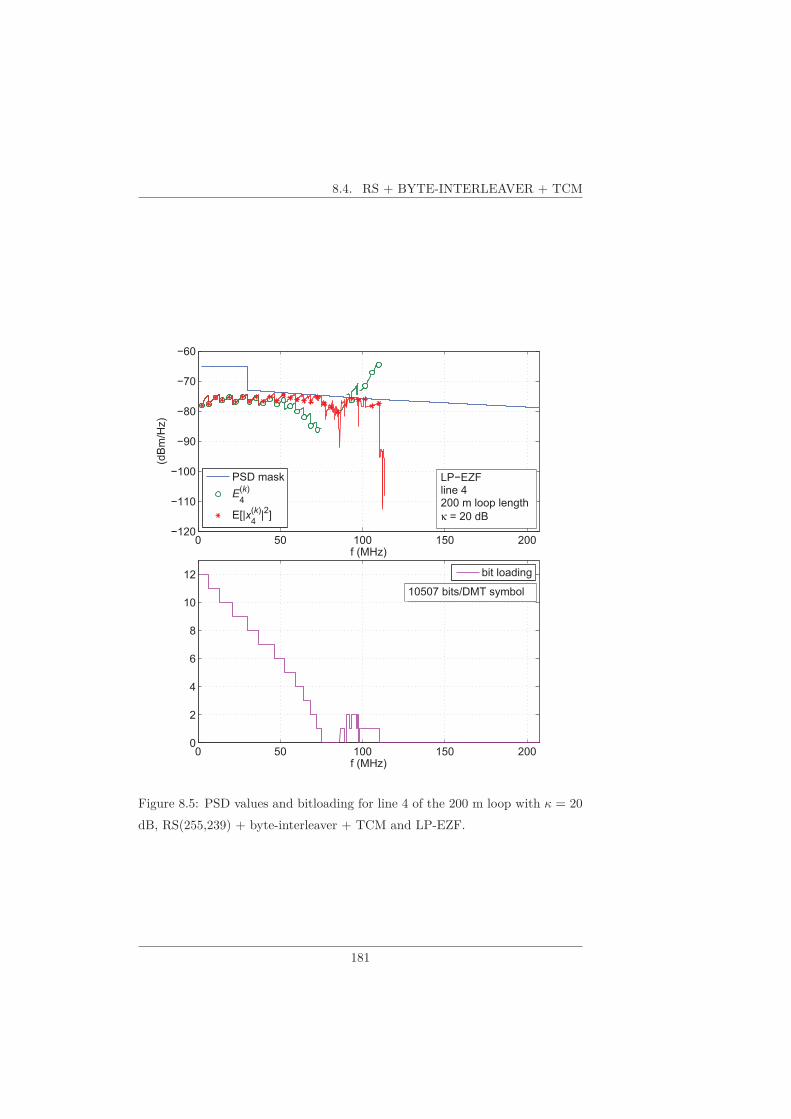
8.4. RS + BYTE-INTERLEAVER + TCM
0 50 100 150 200 120
110
100
90
80
70
60
f!(MHz)
(dBm/Hz)
0 50 100 150 2000
2
4
6
8
10
12
f!(MHz)
PSD!mask
E4
(k)
E[|x4
(k)|2]
bit!loading
10507!bits/DMT!symbol
LP EZFline!4200!m!loop!length
κ!=!20!dB
Figure 8.5: PSD values and bitloading for line 4 of the 200 m loop with κ = 20
dB, RS(255,239) + byte-interleaver + TCM and LP-EZF.
181

8. INFORMATION RATES IN THE PRESENCE OF IMPULSIVE NOISE
Table 8.5: Average information bitrates (Gbps) per line for all proposed LDPC
codes with K = 4320 and NLP-CNS and loop lengths equal to 100 m, 150 m,
200 m and 250 m.
Rc 1/2 2/3 5/6 16/18 20/21
κ = 10 dB
100 m 0.997 1.243 1.449 1.484 1.486
150 m 0.792 0.962 1.079 1.093 1.082
200 m 0.548 0.664 0.738 0.743 0.735
250 m 0.410 0.494 0.558 0.564 0.555
κ = 20 dB
100 m 0.795 0.922 0.993 0.986 0.952
150 m 0.566 0.644 0.682 0.677 0.654
200 m 0.390 0.448 0.485 0.482 0.467
250 m 0.290 0.336 0.361 0.357 0.345
RS(255,239) is only 1.1% and 2.7% larger than for NLP-CNS, for κ = 10 dBand κ = 20 dB, respectively.
For the difference between LP and NLP with RS(255,239); we observe thatNLP outperforms LP by about 15% and 6.4% for CNS and EZF, respectively.
Similar as for the DSL channel without IN, RS(136,120) achieves a loweraverage information bitrate for all loop lenghts and levels of IN. The average in-formation bitrate for RS(255,239) is 5.3% larger than for RS(136,120). Althoughthe RS(136,120) code allows to load more coded bits on the tones, comparedto RS(255,239), the larger parity overhead of the former gives rise to a smallerinformation bitrate.
8.5 Information Rate Comparison
In Figure 8.6, we compare the average information bitrate for all the protectionstrategies considered in this chapter so far, for NLP-EZF and respectively noIN, κ = 10 dB and κ = 20 dB. As far as the LDPC codes is concerned, weonly show the results for the rate 16/18 code (κ = 10 dB) and rate 5/6 code(κ = 20 dB), which performs (nearly) the best for the considered IN levels. Thisconclusion can be generalized over all combinations of precoder and bitloadingalgorithm.
Compared to the case where IN is absent (see Figure 7.11), we observe thatthe presence of IN causes a considerable reduction of the information bitrate,
182

8.5. INFORMATION RATE COMPARISON
Table 8.6: Average information bitrates (Gbps) per line for RS + byte-
interleaving + TCM and IN with κ = 10 dB.
100m 150m 200m 250m
RS(255,239)
LP-EZF 1.338 0.993 0.677 0.513
LP-CNS 1.310 0.848 0.666 0.502
NLP-EZF 1.454 1.064 0.728 0.549
NLP-CNS 1.442 1.051 0.718 0.543
RS(136,120)
LP-EZF 1.269 0.943 0.642 0.487
LP-CNS 1.241 0.804 0.632 0.477
NLP-EZF 1.378 1.010 0.691 0.522
NLP-CNS 1.367 0.998 0.683 0.516
Table 8.7: Average information bitrates (Gbps) per line for RS + byte-
interleaving + TCM and IN with κ = 20 dB.
100m 150m 200m 250m
RS(255,239)
LP-EZF 0.889 0.634 0.448 0.339
LP-CNS 0.800 0.568 0.415 0.272
NLP-EZF 0.959 0.673 0.467 0.348
NLP-CNS 0.941 0.644 0.458 0.340
RS(136,120)
LP-EZF 0.846 0.604 0.426 0.323
LP-CNS 0.760 0.540 0.393 0.258
NLP-EZF 0.912 0.640 0.445 0.331
NLP-CNS 0.895 0.610 0.436 0.323
183
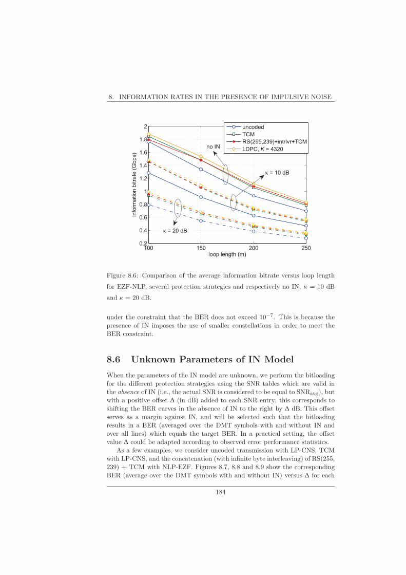
8. INFORMATION RATES IN THE PRESENCE OF IMPULSIVE NOISE
100 150 200 2500.2
0.4
0.6
0.8
1
1.2
1.4
1.6
1.8
2
loop length (m)
info
rmation b
itra
te (
Gbps)
uncoded
TCM
RS(255,239)+intrlvr+TCM
LDPC, K = 4320
κ = 10 dB
no IN
κ = 20 dB
Figure 8.6: Comparison of the average information bitrate versus loop length
for EZF-NLP, several protection strategies and respectively no IN, κ = 10 dB
and κ = 20 dB.
under the constraint that the BER does not exceed 10−7. This is because thepresence of IN imposes the use of smaller constellations in order to meet theBER constraint.
8.6 Unknown Parameters of IN Model
When the parameters of the IN model are unknown, we perform the bitloadingfor the different protection strategies using the SNR tables which are valid inthe absence of IN (i.e., the actual SNR is considered to be equal to SNRavg), butwith a positive offset ∆ (in dB) added to each SNR entry; this corresponds toshifting the BER curves in the absence of IN to the right by ∆ dB. This offsetserves as a margin against IN, and will be selected such that the bitloadingresults in a BER (averaged over the DMT symbols with and without IN andover all lines) which equals the target BER. In a practical setting, the offsetvalue ∆ could be adapted according to observed error performance statistics.
As a few examples, we consider uncoded transmission with LP-CNS, TCMwith LP-CNS, and the concatenation (with infinite byte interleaving) of RS(255,239) + TCM with NLP-EZF. Figures 8.7, 8.8 and 8.9 show the correspondingBER (average over the DMT symbols with and without IN) versus ∆ for each
184

8.6. UNKNOWN PARAMETERS OF IN MODEL
of the 8 lines with DSL loop length 200 m for both κ = 10 dB and κ = 20
dB. We observe that for a given coding scheme, all lines experience virtuallythe same BER. The SNR offsets which yield the target BER of 10−7 on alllines for κ = 10 dB and κ = 20 dB are ∆ = 8.0 dB and ∆ = 13.0 dB foruncoded transmission, ∆ = 8.5 dB and ∆ = 13.5 dB for TCM, and ∆ = 9.2 dBand ∆ = 14.2 dB for RS(255, 239) + TCM. When comparing the SNR tablesfor the case of no IN (i.e., Tables 5.1, 5.2 and 5.12) with those for κ = 10 dB(i.e., Tables 5.6, 5.8 and 5.13) and κ = 20 dB (i.e., Tables 5.6, 5.9 and 5.14), weobserve that the differences in SNR for a given coding scheme and precoder typeare very close to the offset value mentioned above, irrespective of the consideredconstellation; more specifically, for κ = 10 dB and κ = 20 dB, the mean andstandard deviation of these SNR differences are (8.0 dB, 0.05 dB) and (13.0 dB,0.05 dB) for uncoded transmission with LP, (8.5 dB, 0.08 dB) and (13.5 dB,0.05 dB) for TCM with LP, and (9.2 dB, 0.05 dB) and (14.2 dB, 0.05 dB) forRS(255, 239) + TCM with NLP. Hence, when applying the offset mentionedabove to the SNR values from the table pertaining to no IN, we obtain SNRvalues which are very close (within about a tenth of a dB) to the SNR valuesfrom the tables for κ = 10 dB and κ = 20 dB. As a consequence, the bitloadingsresulting from the table pertaining to no IN (after applying the proper offset ∆)yield the same information bitrates as in the case where the parameters of theIN model are known. We have verified that the same observation holds for allcombinations of bitloading algorithms and precoder types.
A similar observation holds for LDPC codes. Comparing the SNR valuesfrom Table 5.11 (valid for the rate 20/21 LDPC code) for no IN with those for κ
= 10 dB and κ = 20 dB, we observe that the mean and standard deviation of thedifferences in SNR are (9.1 dB, 0.04 dB) and (14.1 dB, 0.04 dB), respectively,in the case of LP. This indicates that the bitloading using the SNR values forno IN with an offset of ∆ = 9.1 dB (for κ = 10 dB) or ∆ = 14.1 dB (for κ = 20
dB) gives rise to the corresponding information bitrates from Table 8.5. Thisobservation also holds for other LDPC codes and other combinations of precodertype and bitloading algorithm.
The BER averaged over the DMT symbols with and without IN is upperbounded by the BER related to the DMT symbols with IN. As the instantaneousSNR for the latter DMT symbols equals SNRavg
1+p1κ1+κ , the SNR difference be-
tween the SNR values in the table for no IN and those for a given κ are upper
bounded by 10 log(
1+κ1+p1κ
)
, which amounts to 9.4 dB and 14.5 dB for κ = 10 dB
and κ = 20 dB, respectively. Compared to uncoded transmission and TCM, theoffset values for the LDPC codes and the RS(255, 239) + TCM concatenationare closer to these upper bounds, because the latter coding schemes yield thesteeper BER curves.
185
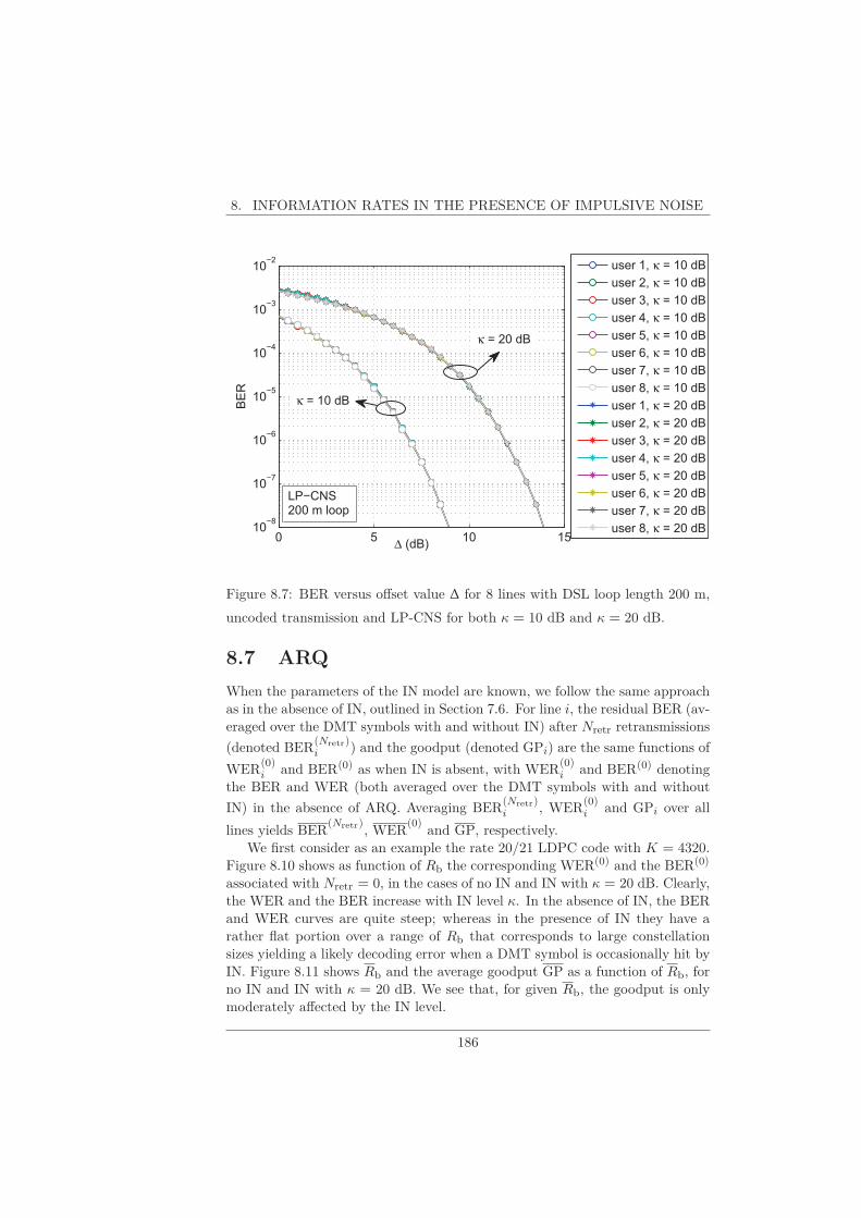
8. INFORMATION RATES IN THE PRESENCE OF IMPULSIVE NOISE
0 5 10 1510
8
10 7
10 6
10 5
10 4
10 3
10 2
∆!(dB)
BER
user!1,!κ!=!10!dB
user!2,!κ!=!10!dB
user!3,!κ!=!10!dB
user!4,!κ!=!10!dB
user!5,!κ!=!10!dB
user!6,!κ!=!10!dB
user!7,!κ!=!10!dB
user!8,!κ!=!10!dB
user!1,!κ!=!20!dB
user!2,!κ!=!20!dB
user!3,!κ!=!20!dB
user!4,!κ!=!20!dB
user!5,!κ!=!20!dB
user!6,!κ!=!20!dB
user!7,!κ!=!20!dB
user!8,!κ!=!20!dB
LP CNS200!m!loop
κ!=!10!dB
κ!=!20!dB
Figure 8.7: BER versus offset value ∆ for 8 lines with DSL loop length 200 m,
uncoded transmission and LP-CNS for both κ = 10 dB and κ = 20 dB.
8.7 ARQ
When the parameters of the IN model are known, we follow the same approachas in the absence of IN, outlined in Section 7.6. For line i, the residual BER (av-eraged over the DMT symbols with and without IN) after Nretr retransmissions
(denoted BER(Nretr)i ) and the goodput (denoted GPi) are the same functions of
WER(0)i and BER(0) as when IN is absent, with WER
(0)i and BER(0) denoting
the BER and WER (both averaged over the DMT symbols with and without
IN) in the absence of ARQ. Averaging BER(Nretr)i , WER
(0)i and GPi over all
lines yields BER(Nretr), WER
(0)and GP, respectively.
We first consider as an example the rate 20/21 LDPC code with K = 4320.Figure 8.10 shows as function of Rb the corresponding WER(0) and the BER(0)
associated with Nretr = 0, in the cases of no IN and IN with κ = 20 dB. Clearly,the WER and the BER increase with IN level κ. In the absence of IN, the BERand WER curves are quite steep; whereas in the presence of IN they have arather flat portion over a range of Rb that corresponds to large constellationsizes yielding a likely decoding error when a DMT symbol is occasionally hit byIN. Figure 8.11 shows Rb and the average goodput GP as a function of Rb, forno IN and IN with κ = 20 dB. We see that, for given Rb, the goodput is onlymoderately affected by the IN level.
186

8.7. ARQ
0 2 4 6 8 10 12 1410
8
10 7
10 6
10 5
10 4
10 3
10 2
∆!(dB)
BER
user!1,!κ!=!10!dB
user!2,!κ!=!10!dB
user!3,!κ!=!10!dB
user!4,!κ!=!10!dB
user!5,!κ!=!10!dB
user!6,!κ!=!10!dB
user!7,!κ!=!10!dB
user!8,!κ!=!10!dB
user!1,!κ!=!20!dB
user!2,!κ!=!20!dB
user!3,!κ!=!20!dB
user!4,!κ!=!20!dB
user!5,!κ!=!20!dB
user!6,!κ!=!20!dB
user!7,!κ!=!20!dB
user!8,!κ!=!20!dBLP CNS200!m!loop
κ!=!20!dB
κ!=!10!dB
Figure 8.8: BERavg versus offset value ∆ for 8 lines with DSL loop length 200
m, TCM and LP-CNS for both κ = 10 dB and κ = 20 dB.
187
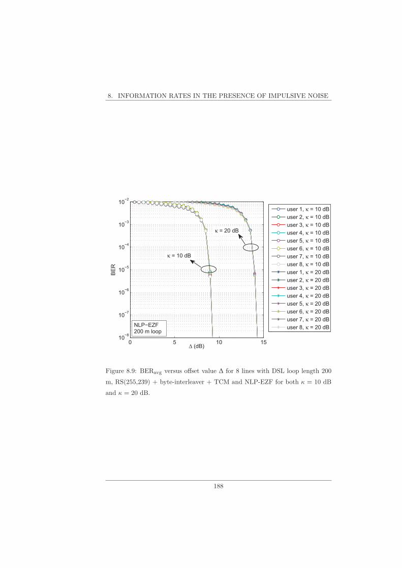
8. INFORMATION RATES IN THE PRESENCE OF IMPULSIVE NOISE
0 5 10 1510
8
10 7
10 6
10 5
10 4
10 3
10 2
∆!(dB)
BER
user!1,!κ!=!10!dB
user!2,!κ!=!10!dB
user!3,!κ!=!10!dB
user!4,!κ!=!10!dB
user!5,!κ!=!10!dB
user!6,!κ!=!10!dB
user!7,!κ!=!10!dB
user!8,!κ!=!10!dB
user!1,!κ!=!20!dB
user!2,!κ!=!20!dB
user!3,!κ!=!20!dB
user!4,!κ!=!20!dB
user!5,!κ!=!20!dB
user!6,!κ!=!20!dB
user!7,!κ!=!20!dB
user!8,!κ!=!20!dBNLP EZF200!m!loop
κ!=!10!dB
κ!=!20!dB
Figure 8.9: BERavg versus offset value ∆ for 8 lines with DSL loop length 200
m, RS(255,239) + byte-interleaver + TCM and NLP-EZF for both κ = 10 dB
and κ = 20 dB.
188

8.7. ARQ
0.8 1 1.2 1.4 1.6 1.8 210
8
10 6
10 4
10 2
100
average Rb (Gbps)
average WER, no IN
average BER, no IN
average WER, κ = 20 dB
average BER, κ = 20 dB
LDPC Rc = 20/21
loop length = 100 m
Figure 8.10: WER(0)
and BER(0)
versus Rb for the rate 20/21 LDPC code with
K = 4320 and Nretr = 0.
0.8 1 1.2 1.4 1.6 1.8 20
0.2
0.4
0.6
0.8
1
1.2
1.4
1.6
1.8
2
average Rb (Gbps)
(Gbps)
average Rb
average GP, no IN
average GP, κ = 20 dB
LDPC Rc = 20/21
loop length = 100 m
Figure 8.11: Rb and GP versus Rb for the rate 20/21 LDPC code with K =
4320.
189

8. INFORMATION RATES IN THE PRESENCE OF IMPULSIVE NOISE
10�8
10�6
10�4
10�2
100
0
0.2
0.4
0.6
0.8
1
1.2
1.4
1.6
1.8
avera
ge G
P (
Gbps)
average residual BER
Nretr
= 0
Nretr
= 1
Nretr
= 2
Nretr
= 3
Nretr
= 4
Nretr
= 5
Nretr
= 6
LDPC Rc = 20/21
loop length = 100 m
κ = 20 dB
Figure 8.12: Average goodput GP versus BER(Nretr) for the rate 20/21 LDPC
code with K = 4320 and various Nretr .
The average goodput GP as a function of the average residual BER, BER(Nretr),
for various Nretr is shown in Figure 8.12 with IN (κ = 20 dB). Comparing Fig-ure 7.12 (no IN) with Figure 8.12 (κ = 20 dB), we see that in the absence ofIN the maxima of the goodput for the various Nretr are broader (because of thesteeper curves of WER(0) versus Rb) and wider apart. In the presence of IN, weneed Nretr,opt = 4 for the considered example to achieve the maximum average
goodput GPopt under the constraint BER(Nretr) ≤ 10−7.
As discussed in Section 5.6, the latency constraint limits the maximum num-ber of retransmissions to Nretr,max = 6. For the considered example, the latencyconstraint does not restrict the average goodput, as Nretr,opt ≤ Nretr,max.
For the different error control strategies and using NLP-CNS, Tables 8.8 and8.9 show GP under the error performance constraint BER ≤ 10−7, for κ = 10
dB and κ = 20 dB, considering the cases of ARQ and no ARQ. For uncodedtransmission and TCM, the information word consists of 4320 bits and theLDPC codes have K = 4320 information bits; for the concatenation of the RSouter code, the infinite byte interleaver and TCM, only the traditional RS(255,239) code is considered. When using ARQ, we distinguish between the caseswhere there is no constraint on Nretr, and where Nretr has to satisfy the latencyconstraint Nretr ≤ Nretr,max, with Nretr,max = 6 (see discussion on latency withARQ in Section 5.6.2). When in the case of ARQ one can achieve, for a specific
190

8.7. ARQ
Table 8.8: Maximum achievable goodput (Gbps) for BER ≤ 10−7 for NLP-CNS
and IN with κ = 10 dB.100 m 150 m 200 m 250 m
κ = 10 dB
uncoded, no ARQ 1.264 0.885 0.613 0.460
uncoded, ARQ 1.684 (3) 1.267 (3) 0.872 (3) 0.657 (3)
TCM, no ARQ 1.435 1.034 0.702 0.532
TCM, ARQ 1.722 (4) 1.332 (4) 0.920 (4) 0.685 (4)
LDPC 1/2, no ARQ 0.997 0.792 0.548 0.410
LDPC 1/2, ARQ 1.070 (4) 0.903 (4) 0.679 (5) 0.508 (5)
LDPC 2/3, no ARQ 1.243 0.962 0.664 0.494
LDPC 2/3, ARQ 1.374 (4) 1.134 (4) 0.822 (5) 0.618 (6)
LDPC 5/6, no ARQ 1.449 1.079 0.738 0.558
LDPC 5/6, ARQ 1.630 (4) 1.317 (4) 0.923 (4) 0.688 (4)
LDPC 16/18, no ARQ 1.484 1.093 0.743 0.564
LDPC 16/18, ARQ 1.706 (4) 1.359 (4) 0.955 (4) 0.711 (4)
LDPC 20/21, no ARQ 1.486 1.082 0.735 0.555
LDPC 20/21, ARQ 1.768 (4) 1.388 (4) 0.970 (4) 0.722 (4)
RS+TCM, no ARQ 1.442 1.051 0.718 0.543
191

8. INFORMATION RATES IN THE PRESENCE OF IMPULSIVE NOISE
Table 8.9: Maximum achievable goodput (Gbps) for BER ≤ 10−7 for NLP-CNS
and IN with κ = 20 dB.100 m 150 m 200 m 250 m
κ = 20 dB
uncoded, no ARQ 0.773 0.513 0.370 0.270
uncoded, ARQ 1.562 (4) 1.123 (4) 0.772 (4) 0.575 (4)
TCM, no ARQ 0.898 0.616 0.441 0.324
TCM, ARQ 1.568 (4) 1.162 (4) 0.783 (4) 0.588 (4)
LDPC 1/2, no ARQ 0.795 0.566 0.390 0.290
LDPC 1/2, ARQ 1.052 (4) 0.903 (5) 0.701 (5) 0.527 (5)
LDPC 2/3, no ARQ 0.922 0.644 0.448 0.336
LDPC 2/3, ARQ 1.322 (4) 1.107 (6) 0.842 (6) 0.635 (6)
LDPC 5/6, no ARQ 0.993 0.681 0.485 0.361
LDPC 5/6, ARQ 1.518 (4) 1.184 (5)0.847 (8)
0.795 (6)
0.637 (8)
0.595 (6)
LDPC 16/18, no ARQ 0.986 0.677 0.482 0.357
LDPC 16/18, ARQ 1.573 (4) 1.204 (5)0.836 (9)
0.801 (6)
0.628 (9)
0.606 (6)
LDPC 20/21, no ARQ 0.952 0.654 0.467 0.345
LDPC 20/21, ARQ 1.616 (4) 1.208 (4) 0.810 (4) 0.611 (4)
RS+TCM, no ARQ 0.941 0.644 0.458 0.340
192
8.7. ARQ
code, GP = GPopt with Nretr,opt ≤ 6, the corresponding entry shows GPoptalong with the value of Nretr,opt. When in the case of ARQ one cannot achieveGP = GPopt with Nretr,opt ≤ 6 for a specific code, the entry shows (i) GPoptalong with the value of Nretr,opt (which is larger than 6); and (ii) the maximumvalue of GP (which is less than GPopt) that can be achieved under the latencyconstraint Nretr ≤ 6 , along with the corresponding Nretr (which equals 6). Foreach loop length, we indicated in the case of ARQ which code yields the largestGP, when the latency constraint applies (marked in bold) or when the latencyconstraint does not apply (marked with underlining); when no ARQ is used, thenumbers in italic indicate which codes achieve the largest GP, for the consideredloop lengths. We make the following observations:
• Comparing Tables 7.9-7.12 (no IN) with Tables 8.8-8.9, we see that whenARQ is used, the amount of IN has a rather small effect (less than about10%) on GPopt, but more retransmissions than in the absence of IN areneeded to achieve GPopt. However, when no ARQ is used, the achievedGP is considerably smaller than GPopt when IN is present, and stronglydependent on the IN level. This indicates that ARQ provides considerablerobustness against IN, at the expense of latency caused by retransmissions.
• Compared to ARQ with proper coding, the traditional concatenation of aRS(255, 239) outer code with a TCM inner code (separated by an infinitebyte interleaver) offers much less protection against IN.
• In the absence of ARQ, (close to) optimum codes are the rate 16/18 andrate 5/6 LDPC codes, for κ = 10 dB and κ = 20 dB, respectively.
• In the presence of ARQ with a latency constraint Nretr ≤ 6, Figure 8.13compares the GP for all the protection strategies considered and respec-tively no IN, κ = 10 dB and κ = 20 dB. As far as LDPC is concerned,we only show the results for the code rate which performs best for theconsidered IN level and loop length. The rate 20/21 LDPC code (4 re-transmissions) is optimum for κ = 10 dB; for κ = 20 dB, the optimumcodes are the rate 20/21 LDPC code (4 retransmissions) for the 100 m and150 m loops, and the rate 2/3 LDPC code (6 retransmission) for the 200 mand 250 m loops, but on these longer loops the rate 20/21 LDPC code (4retransmissions) is only slightly worse than the latter code. No substantialincrease of GP is achieved when removing the latency constraint.
When the parameters of the IN model are not known, one can perform thebitloading using the SNR tables for the case without IN, with an offset addedto the SNR values. When ARQ is used, the offset can be selected such that theaverage goodput is maximized; the number of allowed retransmissions can beselected such that the average residual BER does not exceed the target BER of10−7. When no ARQ is used, the offset can be selected such that the averageBER equals the target BER of 10−7.
193

8. INFORMATION RATES IN THE PRESENCE OF IMPULSIVE NOISE
100 150 200 2500.5
1
1.5
2
loop length (m)
avera
ge G
P (
Gbps)
no IN, uncoded
no IN, TCM
no IN, LDPC Rc = 20/21
κ = 10 dB, uncoded
κ = 10 dB, TCM
κ = 10 dB, LDPC Rc = 20/21
κ = 20 dB, uncoded
κ = 20 dB, TCM
κ = 20 dB, LDPC
Figure 8.13: Comparison of GP versus loop length for CNS-NLP, several pro-
tection strategies and respectively no IN, κ = 10 dB and κ = 20 dB.
194

Part II
Video Transmission over
Wireless Channel
195


9Application Layer ARQ forProtecting Video Packets overan Indoor MIMO-OFDM Linkwith Correlated Block Fad-ing
Published in IEEE Journal on Selected Areas in Communications.
–
The quality of experience (QoE) of IP-packetized streaming video is affectedby both packet loss and packet delay variations. When the network deliveringthe video content contains a wireless link, occasional deep fades give rise tobursts of packet losses. In order to maintain a sufficient video QoE at the enduser, video packets must be protected against losses by means of a suitable formof error control. In this contribution, we consider an indoor radio MIMO-OFDMtransceiver operating over a Rayleigh block-fading channel with arbitrary corre-
197

9. APPLICATION LAYER ARQ FOR PROTECTING VIDEO PACKETSOVER AN INDOOR MIMO-OFDM LINK WITH CORRELATED BLOCKFADING
lation in the time and frequency dimensions, which makes use of an applicationlayer Automatic Repeat reQuest (ARQ) protocol to provide additional protec-tion of the video content against packet loss. We analyze the resulting residualpacket loss performance, under a latency constraint imposed by the requirementof a small TV channel switching delay. This analysis makes direct use of thefading characterization (correlation functions in time and frequency dimensions)of the indoor environment, rather than relying on a Markov model that onlyapproximately describes the packet loss process. Numerical results are obtainedby Monte Carlo integration combined with an efficient importance sampling
technique devised for the problem at hand. Assuming a 2.4 GHz wireless link,
we point out how to select the system parameters (number of antennas, num-
ber of retransmissions) in order to achieve a residual packet loss performance
yielding a satisfactory QoE for HDTV transmission.
9.1 Introduction
The Internet Protocol (IP) allows the provision of a mix of multimedia services
(video, audio, voice, data, gaming, etc.) to an end user, by breaking up the
bit streams generated by the various services into IP packets and sending these
packets over the network. In this part of the dissertation, we consider the
delivery of these multimedia services via a wireless channel, and focus on the
reliability of the received video data.
Wireless channels are frequency-selective and subject to time-varying fading.
These impairments distort the transmitted signal, and give rise to bursts of bit
errors at the receiver when deep fades occur within the signal bandwidth. IP
packets affected by bit errors are erased at the receiver, yielding lost packets
at the destination. In order to achieve a sufficient QoE for (high-quality) video
services, judicious system design should protect the video stream against packet
loss.
The distortion caused by the frequency-selectivity of the channel can be
dealt with by resorting to multicarrier modulation (OFDM) [57], which turns
the frequency-selective channel into a number of parallel frequency-flat channels.
The OFDM signal format has been included in various standards for both wire-
less and wired communications such as ADSL, DVB-T, WiFi and WiMax [58].
Several authors have considered the protection of the video stream against
packet loss by resorting to FEC, to ARQ protocols, or to combinations thereof
(e.g., [59–70]). Most often, in their analysis the packet loss process is described
by a simplified Markov model, which makes abstraction of the fine details of the
underlying phyical processes (fading, noise,. . .) that cause transmission errors,
and, therefore, only approximately captures the packet loss process.
Here, we consider the transmission of a video stream over an indoor radio
channel. The transmitter and receiver are equipped with multiple antennas,
198
9.1. INTRODUCTION
which gives rise to a multiple-input multiple-output (MIMO) wireless channel.The diversity offered by the multiple spatial channels between transmitter andreceiver increases the robustness against fading, e.g., by using space-time blockcodes on the physical (PHY) layer [17–19]. The frequency-selectivity of thechannel is dealt with by adopting the OFDM signal format. The channel isdescribed as Rayleigh block fading, with correlation in both the time and fre-quency dimensions. Additional protection (to the video stream only) is providedby means of selective-repeat ARQ (SR-ARQ) [71, 72], with the number of re-transmissions being restricted by a latency constraint. In order to reduce thecost of the wireless transceiver, the Digital Subscriber Line Access Multiplexer(DSLAM) operates as the retransmitting node. The resulting round-trip timebetween the DSLAM and the wireless receiver is sufficiently small for the SR-
ARQ to be effective; the resulting transmission overhead is considerably smallerthan for FEC, under the same latency constraint [59,61].
In [59], we have investigated to what extent the combination of the RS codeor the SR ARQ protocol with the space-time PHY layer code improves the re-liability of the video transmission over a wireless channel subject to Rayleighfading with frequency-flat transmission channel and independent block fading.We have pointed out that SR-ARQ and RS erasure coding give rise to a diversitygain yielding improved error performance, and have presented simple analyticalexpressions for this gain. Both SR-ARQ and RS erasure coding yield the samemaximum possible diversity gain. However, when using RS erasure coding thismaximum diversity gain cannot be achieved because of practical limitations onthe allowed transmission overhead. The performance analysis assumes that thechannel state is the same for all OFDM subcarriers. This assumption is validwhen the signal bandwidth does not exceed the 90% coherence bandwidth ofthe channel. For the considered 60 GHz indoor radio channel under NLOS con-ditions, the 90% coherence bandwidth is about 6 MHz [73], so that our analysisis valid for bitrates up to 12 Mbit/s (assuming QPSK transmission). When thesignal bandwidth is larger than the 90% coherence bandwidth, different subcar-riers experience different channel states (which could be exploited to increasethe PHY layer diversity by means of frequency-interleaving and coding acrossthe subcarriers of an OFDM block). In this chapter, we use a more generalfading model with correlation in both frequency and time dimensions over a 2.4GHz indoor wireless link and we examine the effect of application layer ARQ.
This chapter is organized as follows. In Section 9.2, we provide a system de-scription involving the packetization of compressed video, the PHY layer of theMIMO-OFDM system, the Rayleigh fading channel model, and the SR-ARQprotocol that protects only the video traffic against packet loss. We provide
in Section 9.3 the packet error performance analysis for various scenarios, for
various combinations of the number of transmit and receive antennas, with or
without additional video packet protection from SR-ARQ, under the assump-
tion of correlated block fading in the time and frequency dimensions. Rather
199

9. APPLICATION LAYER ARQ FOR PROTECTING VIDEO PACKETSOVER AN INDOOR MIMO-OFDM LINK WITH CORRELATED BLOCKFADING
video
server
Aggregation
network
STB+TV
DSL lines
no erasures Rayleigh fading
DSLAM HG+transmitter
wireless
connection
Figure 9.1: Concatenation of DSL connection and wireless connection.
than resorting to a simplified Markov model for describing the packet loss, wemake in our analysis direct use of the fading correlation function in the timeand frequency dimensions. This analysis is a generalization of [59], where afrequency-flat transmission channel with independent block fading was consid-ered. In Section 9.4, we present numerical results, related to High Definition TV(HDTV) [74] transmission over a 2.4 GHz indoor wireless link; these results havebeen obtained by means of an importance sampling technique [75–77], that wedevised for the problem at hand. Finally, in Section 9.5 conclusions are drawnregarding system performance and complexity, and some remarks are formu-lated regarding the use, in the considered system, of additional video protectionby means of FEC rather than SR-ARQ. A major conclusion is that SR-ARQyields diversity gain, which is limited by the ratio of the allowed latency andthe time interval between retransmissions, at the expense of only a very smalltransmission overhead.
9.2 System Description
We consider the case where video content is sent from the video server to theend user, as shown in Figure 9.1. A source, the video server, broadcasts thevideo data. Via an aggregation network, this video data reaches a DSLAM.The DSLAM sends the data related to a mix of services (video, audio, voice,data, gaming, etc.), over a Digital Subscriber Line (DSL) [78] to the user HomeGateway (HG). From the HG, the video data is sent through a wireless LAN tothe Set Top Box (STB).
The video stream is encoded (compressed) by exploiting the temporal andspatial redundancy that is present in uncompressed video frames [16, 79, 80].The resulting Transport Stream (TS) consists of a sequence of MPEG-TS pack-ets, each containing 188 bytes (including a 4-byte header). For transmissionover IP networks, 7 MPEG-TS packets (together with header information) areencapsulated in an IP packet [81].
On the Medium Acces Control (MAC) sublayer of the data link layer, a
200

9.2. SYSTEM DESCRIPTION
Cyclic Redundancy Check (CRC) is added. This CRC allows the detection ofpackets that are corrupted by transmission errors; corrupted packets are notforwarded to the network layer, but are discarded (’erased’) and therefore con-sidered as lost. We assume there are no data link layer retransmissions (becausethe adverse affect of fading is reduced by means of space-time channel codingon the physical layer). Considering the sizes of the payload (7 TS packets) andof the headers/trailers added by the various protocol layers, the MAC packetsarriving at the HG have a size of 1374 byte (10992 bit).
As far as the physical (PHY) layer is concerned, we only consider the wirelesslink between the HG and the STB. On the PHY layer of the HG transmitter, theL bits to be sent for every data-link-layer packet are mapped onto an M -pointsignal constellation. The resulting M -ary data symbols are transmitted at a rateRs (in symbols per second) over the wireless channel; hence the duration of apacket equals L/(Rs log2(M )). The transmission makes use of OFDM [57]. Thesequence of data symbols at rate Rs is demultiplexed into Nt parallel symbolstreams, each of rate Rs/Nt. These Nt symbol streams are modulated onto Nt
distinct tones, that have a frequency separation of (slightly more than) Rs/Nt,and the sum of these modulated tones is transmitted. The transmitted signalcan be viewed as a sequence of OFDM blocks, each having a duration of Nt/Rs,and containing Nt data symbols (i.e., one symbol on each of the Nt tones).The bandwidth occupied by the resulting transmitted signal is (slightly morethan) Rs. The transmission of an L-bit packet involves L/(Nt log2(M )) OFDMblocks. The OFDMmodulation turns the frequency-selective fading channel intoa set of Nt flat-fading parallel channels.
Each tone of the OFDM system is affected by slow frequency-flat Rayleighfading, and the fading on different tones is correlated. We restrict our attentionto the case where the channel coherence time and the channel coherence band-width are much larger than the packet duration L/(Rs log2(M )) and the tonespacing Rs/Nt, respectively. Therefore, we assume that
• the fading gain on a given tone is constant over the packet duration, andthe fading gains are correlated from one packet to the next.
• there are NF sets of Nt/NF consecutive tones, with all tones within asame set experiencing the same fading gain, and the fading gains beingcorrelated from one set to the next.
This fading model corresponds to correlated block fading in both time andfrequency.
On the PHY layer of the STB receiver, the M -ary data symbols are detected,and demapped to bits. On the MAC sublayer, the recovered bits are groupedinto packets of size L, and error detection based on the CRC is performed.When an error is detected, the packet is erased; otherwise, the packet is passedto the higher layers.
201

9. APPLICATION LAYER ARQ FOR PROTECTING VIDEO PACKETSOVER AN INDOOR MIMO-OFDM LINK WITH CORRELATED BLOCKFADING
Because of fading, some of the tone signals are occasionally strongly at-tenuated. To alleviate the damaging impact of fading on the detection of theM -ary data symbols, some form of channel coding is used on the PHY layer:the transmitter introduces some redundancy in the time, frequency and/or spa-tial dimensions, that is exploited at the receiver to correct transmission errors.In this chapter, we consider the use of multiple transmit and receive anten-nas. A MIMO system with Ntr transmit and Nr receive antennas allows theintroduction of space-time coding as discussed in more detail in Section 2.4.
All multimedia services that make use of the wireless link benefit from theprotection against fading, provided by the PHY layer diversity NtrNr. However,this protection might not be sufficient for achieving a sufficient QoE for video
services. The relation between packet error performance and QoE is rather
complicated: on one hand the video decoder has error concealment capabilities,
but on the other hand the effect of a single packet loss might propagate; the
interested reader is referred to [70, 82–86]. In this paper, we rely on the rec-
ommendation [87], which states that, for several video compression standards
(i.e., MPEG-2, H.264/AVC and VC-1), IP packet loss should be limited to at
most one error event per hour for Standard Definition TV (SDTV) and to one
error event per four hours for HDTV, with an error event being defined as the
loss of a small number of IP packets; for HDTV it is estimated that only one
out of three error events will yield a visible impairment (because of the error
concealment techniques), so that on average only one visual distorsion in 12
hours would result.
We consider in this paper additional protection by means of application
layer retransmissions, applied exclusively to the video packets. We restrict our
attention to SR-ARQ, which involves the retransmission (upon request from the
STB receiver) of copies of only the lost packets, with the retransmitting node
not waiting for acknowledgement before transmitting a next packet [71,72].
The time interval Tretr between (re)transmission instants of the same packet
is the sum of the packet duration L/(Rs log2(M )) and the round-trip delayTRTT ; the latter is the sum of the two-way propagation delay, the duration
of the acknowledgment message, and the processing delays at the receiver and
the transmitter as given in (2.15). Since each retransmission gives rise to a
latency of Tretr, the maximum latency introduced by the SR-ARQ protocol
equals NretrTretr, with Nretr denoting the maximum number of retransmissions
per packet. The latency caused by the SR-ARQ protocol contributes to the TV
channel switching delay. In order to achieve acceptable values for this delay,
the latency should be limited. Therefore, we select as the retransmitting node
the DSLAM rather than the video source, because the former yields the smaller
round-trip delay. Of course, the retransmitting network node needs sufficient
intelligence, in order to handle retransmission requests related to specific video
packets; in addition, this node must have a retransmission buffer containing
video packets that have not yet been correctly received by the STB. Augment-
202

9.3. SYSTEM ANALYSIS
ing the functionality of the DSLAM increases its complexity and cost. Onecould also envisage to use the HG as retransmitting node. As the HG is a con-sumer product, the DSLAM appears to be the economically justified choice foroperating as the retransmitting node. However, the HG would offer the shorterround-trip delay.
9.3 System Analysis
In this section, we present the analysis of the system under study. We derivethe probability of unrecoverable packet loss, and investigate the burstiness ofthe unrecoverable packet losses. As a performance measure, we consider theaverage number of bursts of unrecoverable packet losses, over a reference timeinterval.
Assuming that the number (L/ log2(M )) of symbols per packet is muchlarger than the number (Nt) of OFDM tones, for a MIMO-OFDM system usingNtr transmit and Nr receive antennas, there are NtrNrNF fading gains involvedin the transmission of single packet; NF denotes the number of tone sets, with allNt/NF tones in a given set experiencing the same fading gain. These NtrNrNF
fading gains determine the channel state vector v(l) of dimension NF, relatedto the considered packet indexed by l. The mth component of v(l) is given by
vm(l) =Ntr∑
i=1
Nr∑
j=1
∣∣∣h
(i,j)m (l)
∣∣∣
2m = 1, . . . ,NF (9.1)
where h(i,j)m (l) is the complex fading gain related to the mth tone set on the link
between the ith transmit antenna and the jth receive antenna. The fading gains
are normalized, such that E[|h(i,j)m (l)|2] = 1. Fading gains related to different
pairs (i, j) are statistically independent. Each of the Nr received signals isaffected by additive white Gaussian noise. The noise contributions at differentantennas, on different tones and in different symbol intervals are statisticallyindependent.
Considering SR-ARQ with a maximum of Nretr retransmissions, an unre-coverable packet loss occurs when the first transmission and all Nretr retrans-missions of a packet are erased. Hence, an unrecoverable packet loss involvesNretr + 1 channel state vectors, which we denote v(0), . . . ,v(Nretr). For givenchannel state vectors, the probability of an unrecoverable packet loss is givenby
Punrec(v(0), . . . ,v(Nretr)) =Nretr∏
l=0
Pp,e(v(l)) (9.2)
where Pp,e(v(l)) is the probability that the lth copy of the considered packet iserased (l = 0, . . . ,Nretr). The probability Pp,e(v(l)) equals the probability that
203

9. APPLICATION LAYER ARQ FOR PROTECTING VIDEO PACKETSOVER AN INDOOR MIMO-OFDM LINK WITH CORRELATED BLOCKFADING
at least one data symbol from the packet is detected in error:
Pp,e(v(l)) = 1−NF∏
m=1
(1− Ps(vm(l))
)KF (9.3)
where Ps(vm(l)) is the probability that a symbol, transmitted on a tone be-longing to the mth tone set, is detected in error, while KF = L/(NF log2(M ))denotes the number of symbols transmitted per tone set and per packet. Theprobability Ps(vm(l)) depends on the symbol constellation and on the type ofspace-time coding. For a QPSK constellation one obtains
Pp,e(v(l)) = 1−NF∏
m=1
(1−BER(vm(l))
)L/NF (9.4)
with BER(vm(l)) denoting the bit error probability [17–20]:
BER(vm(l)) = Q
√
2Ebηvm(l)
N0
(9.5)
In (9.5), Eb denotes the received energy per bit of the video packet; N0 is theone-sided power spectral density of the noise at the receiver; η = 1 for uncodedtransmission (Ntr = 1) and η = 1/2 for Alamouti space-time coding (Ntr = 2);Q(u) is the complement of the cumulative distribution function of a zero-meanunit-variance Gaussian random variable.
The average probability of an unrecoverable packet error is obtained byaveraging (9.2) over the joint distribution of the Nretr + 1 channel state vectorsv(0), . . . ,v(Nretr):
Punrec,p = E[Punrec(v(0), . . . ,v(Nretr))] (9.6)
As the channel state vectors are correlated, it appears impossible to obtain aclosed-form expression for Punrec,p.
Although a closed-form expression for Punrec,p is not available, we will nowpoint out that Punrec,p is proportional to (Eb/N0)−D at high Eb/N0, and de-termine the value of D. Let us consider a bit error pattern containing Nb biterrors, that gives rise to an unrecoverable packet loss. With each erroneousbit are associated NtrNr complex-valued Rayleigh fading gains. Stacking allNbNtrNr fading gains related to the erroneous bits into a vector h, we de-note by r the rank of the autocorrelation matrix of h. It can be shown that,for increasing Eb/N0, the probability of occurrence of the considered bit errorpattern, averaged over the fading gains, is proportional to (Eb/N0)−d, withd = NtrNrr [20]. The dominating bit error patterns yielding unrecoverablepacket loss are those for which the rank r of the associated correlation matrixis minimum. As an unrecoverable packet loss implies that at least one bit in
204

9.3. SYSTEM ANALYSIS
each of the Nretr + 1 copies of the considered packet must be in error (and thecorresponding fading gains are assumed to have a full rank correlation matrix),the minimum rank equals Nretr + 1. Hence, at high Eb/N0, Punrec,p is pro-portional to (Eb/N0)−D, with D = (Nretr + 1)NtrNr denoting the diversityorder. Hence, the number of transmit antennas, the number of receive antennasand the number of retransmissions all contribute positively to the diversity or-der; therefore, increasing any of these quantities gives rise to a steeper negativeslope of Punrec,p as a function of Eb/N0. When no ARQ is used (i.e., Nretr = 0),the resulting diversity order equals the spatial diversity order NtrNr offered bythe MIMO system [17–19]. Hence, the introduction of SR-ARQ increases thediversity by a factor of Nretr + 1 as compared to the PHY layer diversity.
Because of the temporal correlation of the fading, the packet losses tendto occur in bursts: typically, relatively short intervals containing packet lossesare followed by relatively long intervals without packet losses, and vice versa.Let us denote by n the number of lost packets in an interval of N inter-packetintervals; it is to be understood that a packet is lost when it has been erasedduring its transmission and its Nretr retransmissions. We consider the averagenumber E[n|n > 0] of packets in an interval of length Nint that contains at leastone lost packet, which can be computed as
E[n|n > 0] =E[n]
1−Pr[n = 0]=
Nint · Punrec,p
1−Pr[n = 0](9.7)
Clearly, E[n|n > 0] increases with Nint. However, when Nint ranges between(roughly) the average burst size and the average number of packets betweenbursts, an interval of size Nint that is affected by packet loss typically containsa single burst of lost packets, so that E[n|n > 0] is essentially constant withinthis range of Nint and equal to the average number Nburst of lost packets perburst. Hence, examination of E[n|n > 0] as a function of Nint reveals the valueof Nburst. The average number of unrecoverable packet losses in a long referenceinterval containing Nref inter-packet intervals equals NrefPunrec,p. The averagenumber of bursts of unrecoverable packet losses in this interval of size Nref thenequals NrefPunrec,p/Nburst.
Let us investigate the average overhead E[ovh] related to the retransmissionprotocol. The average number E[#transm] of transmissions per packet is relatedto the average overhead by E[#transm] = 1+ E[ovh]. It is easily verified that
E[#transm] = 1+Nretr∑
i=1
Pr[#transm > i] (9.8)
The quantity Pr[#transm > i] can be expressed as
Pr[#transm > i] = E
[i−1∏
l=0
Pp,e(v(l))
]
(9.9)
205
9. APPLICATION LAYER ARQ FOR PROTECTING VIDEO PACKETSOVER AN INDOOR MIMO-OFDM LINK WITH CORRELATED BLOCKFADING
It follows from (9.2) that Pr[#transm > i] in (9.9) can be interpreted as theaverage probability of unrecoverable packet loss for SR-ARQ with a maximum ofi − 1 retransmissions, which at high Eb/N0 is proportional to (Eb/N0)−iNtrNr .Hence, the dominating contribution to E[ovh] = E[#transm] − 1 is the termPr[#transm > 1] = E[Pp,e(v(0))], which at high Eb/N0 is proportional to(Eb/N0)−NtrNr . Therefore, E[ovh] is determined mainly by the PHY layerdiversity.
9.4 Numerical Results
We consider the transmission of compressed HDTV according to the configura-tion shown in Figure 9.1. The compressed video bitrate equals 7.5 Mbps. Themaximum allowed latency introduced by the SR-ARQ protocol is set at 200 ms.The error performance target is an average number of at most one unrecover-able packet burst per 4 hours [87]. The DSLAM acts as retransmitting node;the corresponding interval (Tretr) between retransmission instants is about 50ms [88, 89], so the maximum number (Nretr) of retransmissions meeting the la-tency constraint is 4. The required retransmission buffer size is TretrNretrRp
packets, which amounts to about 150 video packets or 1.5 Mbit when Nretr = 4.The link between the HG and the STB is a 2.4 GHz indoor wireless con-
nection [90] with a bandwidth of 20 MHz; assuming nonline-of-sight (NLOS)conditions, this connection is modeled as a Rayleigh fading channel, with aDoppler spread fD equal to 8 Hz (corresponding to a speed of motion of about1 m/s). We assume that the Doppler spectrum SD(f) has a Gaussian shape:
SD(f) =1√2πσF
exp
(−f2
2σ2F
)
(9.10)
with σF = fD/4 (so that SD(fD) is negligibly small as compared to SD(0)).The resulting time-correlation RD(u) is the inverse Fourier transform of SD(f):
RD(u) = exp(−2π2σ2Fu2) (9.11)
The power delay profile of the indoor channel is assumed to be exponentiallydecaying with a time constant τ of 30 ns. The correlation RH(∆F ) between twochannel transfer function values at f and f + ∆f is the Fourier transform of thepower delay profile:
RH(∆f) =1
1+ j2πτ∆f(9.12)
We split the channel bandwidth BRF into NF subbands of width BRF/NF. Thecorrelation between channel transfer functions at the center and the edge of asubband equals RH(BRF/(2NF)). We select NF such that |RH(BRF/(2NF))| ≥0.9, so that all OFDM subcarriers in a subband experience essentially the samefading as the subcarrier at the center of the subband. For τ= 30 ns and BRF =
206
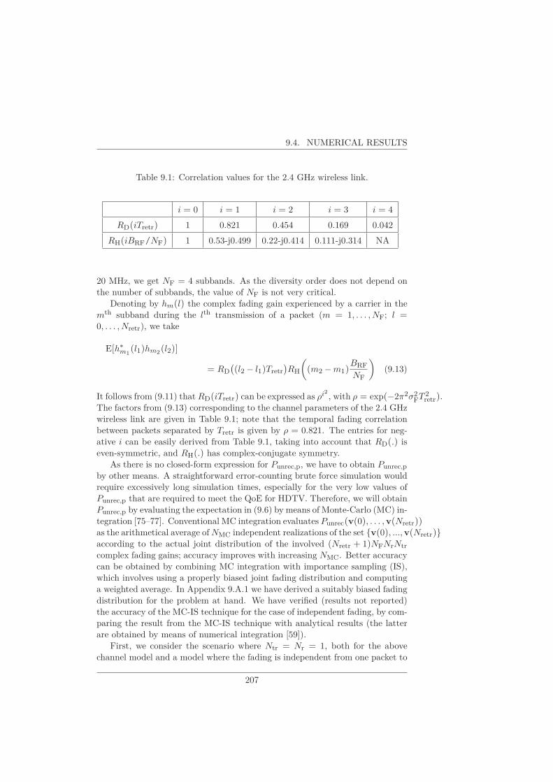
9.4. NUMERICAL RESULTS
Table 9.1: Correlation values for the 2.4 GHz wireless link.
i = 0 i = 1 i = 2 i = 3 i = 4
RD(iTretr) 1 0.821 0.454 0.169 0.042
RH(iBRF/NF) 1 0.53-j0.499 0.22-j0.414 0.111-j0.314 NA
20 MHz, we get NF = 4 subbands. As the diversity order does not depend onthe number of subbands, the value of NF is not very critical.
Denoting by hm(l) the complex fading gain experienced by a carrier in themth subband during the lth transmission of a packet (m = 1, . . . ,NF; l =0, . . . ,Nretr), we take
E[h∗m1
(l1)hm2(l2)]
= RD
((l2 − l1)Tretr
)RH
(
(m2 − m1)BRF
NF
)
(9.13)
It follows from (9.11) that RD(iTretr) can be expressed as ρi2 , with ρ = exp(−2π2σ2FT 2retr).
The factors from (9.13) corresponding to the channel parameters of the 2.4 GHzwireless link are given in Table 9.1; note that the temporal fading correlationbetween packets separated by Tretr is given by ρ = 0.821. The entries for neg-ative i can be easily derived from Table 9.1, taking into account that RD(.) iseven-symmetric, and RH(.) has complex-conjugate symmetry.
As there is no closed-form expression for Punrec,p, we have to obtain Punrec,pby other means. A straightforward error-counting brute force simulation wouldrequire excessively long simulation times, especially for the very low values ofPunrec,p that are required to meet the QoE for HDTV. Therefore, we will obtainPunrec,p by evaluating the expectation in (9.6) by means of Monte-Carlo (MC) in-tegration [75–77]. Conventional MC integration evaluates Punrec(v(0), . . . ,v(Nretr))as the arithmetical average of NMC independent realizations of the set {v(0), ...,v(Nretr)}according to the actual joint distribution of the involved (Nretr + 1)NFNrNtr
complex fading gains; accuracy improves with increasing NMC. Better accuracycan be obtained by combining MC integration with importance sampling (IS),which involves using a properly biased joint fading distribution and computinga weighted average. In Appendix 9.A.1 we have derived a suitably biased fadingdistribution for the problem at hand. We have verified (results not reported)the accuracy of the MC-IS technique for the case of independent fading, by com-paring the result from the MC-IS technique with analytical results (the latterare obtained by means of numerical integration [59]).
First, we consider the scenario where Ntr = Nr = 1, both for the abovechannel model and a model where the fading is independent from one packet to
207

9. APPLICATION LAYER ARQ FOR PROTECTING VIDEO PACKETSOVER AN INDOOR MIMO-OFDM LINK WITH CORRELATED BLOCKFADING
0 5 10 15 20 25 30 35 4010
10
10 8
10 6
10 4
10 2
100
Eb/N
0!(dB)
Punrec,p
!Nretr!=!0
ρ!=!0,!Nretr!=!2
ρ!=!0,!Nretr!=!4
ρ!=!0.821,!Nretr!=!2
ρ!=!0.821,!Nretr!=!4
Ntr!=!1
Nr!=!1
Figure 9.2: Punrec,p with and without temporal fading correlation.
the next (the latter case corresponds to replacing in (9.13) RD((l2 − l1)Tretr) bya Kronecker delta δ(l2 − l1)). Figure 9.2 shows the corresponding Punrec,p, forNretr = 0, 2, 4. We observe that the temporal correlation of the fading gives riseto performance degradation, as compared to the case of uncorrelated fading.This can be understood by noting that, when the first transmission of a packetis not successful because of deep fading, the probability that the retransmissionsof that packet also experience deep fading is larger when the fading is correlatedover time, as compared to uncorrelated fading. This observation illustrates theimportance of taking temporal correlation of the fading into account.
We have computed Punrec,p as a function of Eb/N0 for Nretr ranging from0 to 4, taking the temporal correlation of the fading process into account. Wehave considered the scenarios (Ntr,Nr) = (1, 1), (1, 2), (2, 1) and (2, 2), forwhich the results are shown in Figures 9.3-9.6. The following observation canbe made:
1. For the different scenarios, the high-Eb/N0 behavior of Punrec,p confirmsthat the diversity order is indeed equal to NtrNr(Nretr + 1), as can beverified from the slopes of the curves at high Eb/N0.
2. The use of SR-ARQ gives rise to a considerable performance improvementas compared to the case Nretr = 0. The performance gain resulting from
208

9.4. NUMERICAL RESULTS
0 5 10 15 20 25 30 35 4010
10
10 8
10 6
10 4
10 2
100
Eb/N
0!(dB)
Punrec,p
Nretr!=!0
Nretr!=!1
Nretr!=!2
Nretr!=!3
Nretr!=!4
Figure 9.3: Punrec,p for (Ntr,Nr) = (1, 1) and ρ = 0.821.
one additional retransmission decreases with increasing Nretr.
According to the method outlined in Section 9.3, we have determined theaverage number Nburst of unrecoverable packets per error burst, along with theaverage number of error bursts in a reference period of 4 hrs, for the variousscenarios.
The performance results for the channel with time-correlated fading are sum-marized in Table 9.2 and Table 9.3, which for the several scenarios indicate theaverage number of unrecoverable packet losses per error burst and the value ofEb/N0 at which the average number of error bursts in 4 hrs equals 1 (which isthe performance target for HDTV [87]). Note that in order to achieve satisfac-tory performance, one can trade-off the hardware cost (increasing with numberof transmit and receive antennas) of the wireless transceiver versus the increasedlatency and DSLAM retransmission buffer size (increasing with Nretr); note thatall types of multimedia traffic benefit from an increase of the number of anten-
nas, whereas the SR-ARQ is applied only to the video traffic.
Finally, we investigate the average transmission overhead E[ovh] of the SR-protocol with time-correlated fading. Figure 9.7 shows the average overhead
as a function of Eb/N0, for various combinations of (Ntr,Nr,Nretr). At highEb/N0, the average overhead is mainly equal to Pp,e,avg (which is obtained by
averaging Pp,e(v(l)) over the associated fading gains), and, therefore, is only
209

9. APPLICATION LAYER ARQ FOR PROTECTING VIDEO PACKETSOVER AN INDOOR MIMO-OFDM LINK WITH CORRELATED BLOCKFADING
0 5 10 15 20 25 30 35 4010
10
10 8
10 6
10 4
10 2
100
Eb/N
0!(dB)
Punrec,p
Nretr!=!0
Nretr!=!1
Nretr!=!2
Nretr!=!3
Nretr!=!4
Figure 9.4: Punrec,p for (Ntr,Nr) = (1, 2) and ρ = 0.821.
Table 9.2: Average number of unrecoverable packet losses per error burst.
Nburst @ E[#unrec. bursts in 4 hr] = 1
Nretr = 0 Nretr = 1 Nretr = 2 Nretr = 3 Nretr = 4
Ntr = 1, Nr = 1 1 1.8 3.4 4.0 3.8
Ntr = 1, Nr = 2 1.3 3.2 3.1 2.9 3.1
Ntr = 2, Nr = 1 1.3 3.2 3.0 2.9 3.1
Ntr = 2, Nr = 2 2.6 2.4 2.3 2.2 2.2
210

9.4. NUMERICAL RESULTS
0 5 10 15 20 25 30 35 4010
10
10 8
10 6
10 4
10 2
100
Eb/N
0!(dB)
Punrec,p
Nretr!=!0
Nretr!=!1
Nretr!=!2
Nretr!=!3
Nretr!=!4
Figure 9.5: Punrec,p for (Ntr,Nr) = (2, 1) and ρ = 0.821.
Table 9.3: Performance summary.
Eb/N0 @ E[#unrec. bursts in 4 hr] = 1
no ARQ Nretr = 1 Nretr = 2 Nretr = 3 Nretr = 4
Ntr = 1, Nr = 1 78.5 dB 45.8 dB 35.8 dB 31.4 dB 28.2 dB
Ntr = 1, Nr = 2 42.0 dB 26.8 dB 22.4 dB 20.2 dB 18.3 dB
Ntr = 2, Nr = 1 45.0 dB 29.8 dB 25.4 dB 23.2 dB 21.3 dB
Ntr = 2, Nr = 2 25.3 dB 19.3 dB 17.0 dB 15.1 dB 13.7 dB
211

9. APPLICATION LAYER ARQ FOR PROTECTING VIDEO PACKETSOVER AN INDOOR MIMO-OFDM LINK WITH CORRELATED BLOCKFADING
0 5 10 15 20 25 30 3510
10
10 8
10 6
10 4
10 2
100
Eb/N
0!(dB)
Punrec,p
Nretr!=!0
Nretr!=!1
Nretr!=!2
Nretr!=!3
Nretr!=!4
Figure 9.6: Punrec,p for (Ntr,Nr) = (2, 2) and ρ = 0.821.
weakly dependent on Nretr; this is because when the first transmission of apacket fails, the first retransmission is much more likely to be correctly receivedthan to be erased. For the Eb/N0 values from Table 9.3, E[ovh] is always lessthan 10−3.
9.5 Conclusions and Remarks
In this Chapter, we have analyzed an OFDM system for video transmissionover a Rayleigh fading frequency-selective MIMO wireless link, with space-timecoding on the PHY layer and additional protection against video packet lossby means of application layer SR-ARQ. Our theoretical findings have been il-lustrated in a case study involving HDTV transmission over a 2.4 GHz indoorwireless link, with severe restrictions on latency and on residual packet loss rate.In order to obtain accurate numerical results within reasonable computing time,a suitable importance sampling technique has been devised. The conclusions ofour work can be summarized as follows.
1. SR-ARQ gives rise to a diversity gain, yielding improved error perfor-mance. The resulting diversity order equals (Nretr + 1)NtrNr.
212
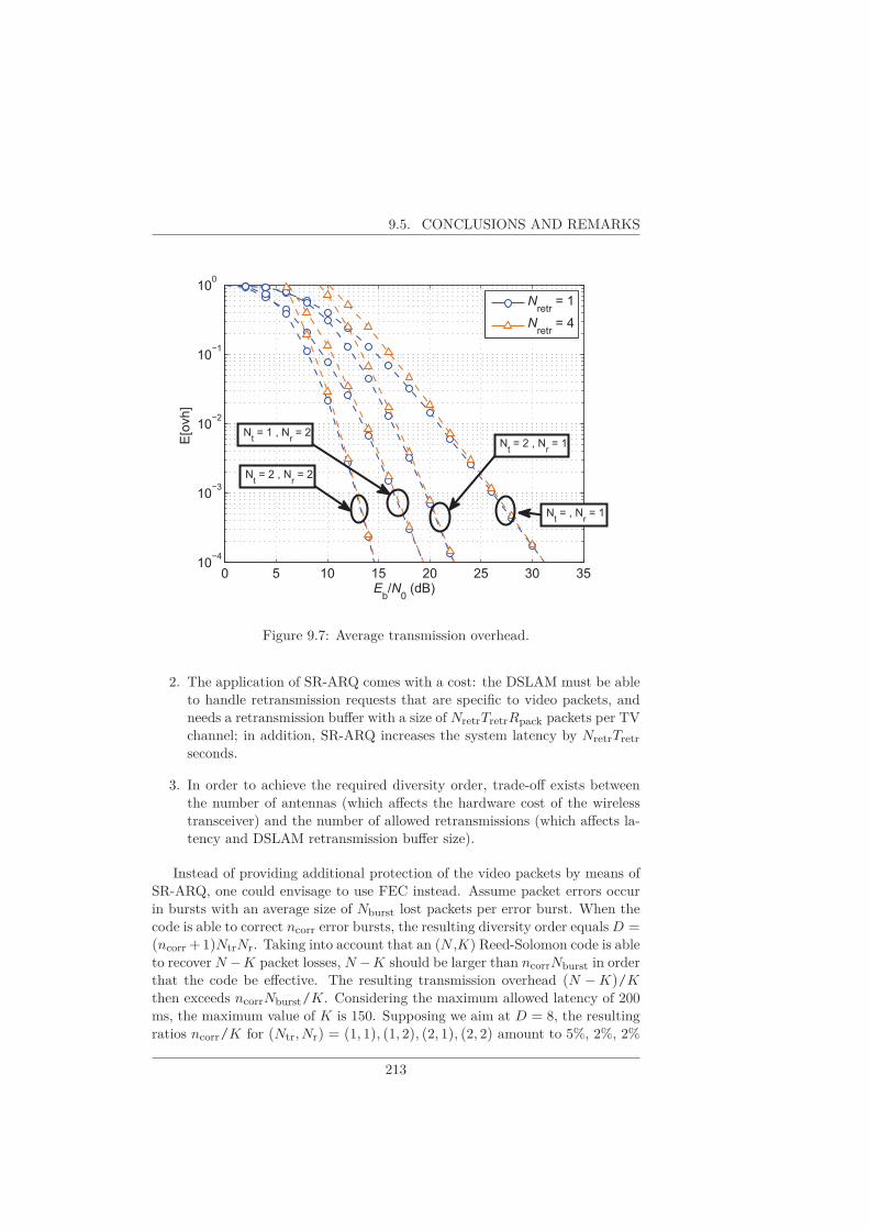
9.5. CONCLUSIONS AND REMARKS
0 5 10 15 20 25 30 3510
4
10 3
10 2
10 1
100
Eb/N
0!(dB)
E[ovh]
Nretr!=!1
Nretr!=!4
!Nt!=!2!,!N
r!=!1
!Nt!=!,!N
r!=!1
!Nt!=!1!,!N
r!=!2
!Nt!=!2!,!N
r!=!2
Figure 9.7: Average transmission overhead.
2. The application of SR-ARQ comes with a cost: the DSLAM must be ableto handle retransmission requests that are specific to video packets, andneeds a retransmission buffer with a size of NretrTretrRpack packets per TVchannel; in addition, SR-ARQ increases the system latency by NretrTretrseconds.
3. In order to achieve the required diversity order, trade-off exists betweenthe number of antennas (which affects the hardware cost of the wirelesstransceiver) and the number of allowed retransmissions (which affects la-tency and DSLAM retransmission buffer size).
Instead of providing additional protection of the video packets by means ofSR-ARQ, one could envisage to use FEC instead. Assume packet errors occurin bursts with an average size of Nburst lost packets per error burst. When thecode is able to correct ncorr error bursts, the resulting diversity order equals D =(ncorr+ 1)NtrNr. Taking into account that an (N ,K) Reed-Solomon code is ableto recover N − K packet losses, N − K should be larger than ncorrNburst in orderthat the code be effective. The resulting transmission overhead (N − K)/K
then exceeds ncorrNburst/K. Considering the maximum allowed latency of 200ms, the maximum value of K is 150. Supposing we aim at D = 8, the resultingratios ncorr/K for (Ntr,Nr) = (1, 1), (1, 2), (2, 1), (2, 2) amount to 5%, 2%, 2%
213

9. APPLICATION LAYER ARQ FOR PROTECTING VIDEO PACKETSOVER AN INDOOR MIMO-OFDM LINK WITH CORRELATED BLOCKFADING
and 0.7%, respectively. Hence, the overheads introduced by FEC are muchhigher than for ARQ.
214

9.A. APPENDIX
9.A Appendix
9.A.1 Monte Carlo Integration with Importance Sampling
Let us consider the expectation of a function F (w) of a random vector w, withprobability density function (pdf) p(w):
Ep[F (w)] =
∫
F (w)p(w)dw (9.14)
The subscript of the expectation operator refers to the pdf of w. When theintegral in (9.14) is difficult to evaluate analytically or numerically, we can
obtain Ep[F (w)] by means of Monte-Carlo integration.Conventional Monte-Carlo integration involves approximating Ep[F (w)] as
Ep[F (w)] ≈ 1
NMC
NMC∑
k=1
F (wk) (9.15)
where the vectors wk are generated independently according to the pdf p(w).Any degree of accuracy can be obtained by taking N sufficiently large.
The accuracy of conventional Monte-Carlo integration can be improved by
means of importance sampling. Importance sampling is based on the transfor-
mation of (9.14) into
Ep[F (w)] =
∫
F (w)p(w)
q(w)q(w)dw (9.16)
where q(w) is also a pdf. From (9.16) the following Monte-Carlo integrationmethod can be derived:
Ep[F (w)] = Eq
[
F (w)p(w)
q(w)
]
≈ 1
NMC
NMC∑
k=1
F (wk)p(wk)
q(wk)(9.17)
where the vectors wk are generated independently according to the pdf q(w).Note that (9.17) reduces to conventional Monte-Carlo integration (9.15) when
q(w) = p(w). The choice of q(w) affects the accuracy of the approximation(9.17); the mean-square approximation error resulting from (9.17) is given by:
Eq
[∣∣∣∣
1
NMC
NMC∑
k=1
F (wk)p(wk)
q(wk)−Ep[F (w)]
∣∣∣∣
2]
=1
NMC
((∫
F 2(w)p2(w)
q(w)dw
)
− (Ep[F (w)])2)
(9.18)
Selecting
q(w) = C F (w)p(w) (9.19)
215

9. APPLICATION LAYER ARQ FOR PROTECTING VIDEO PACKETSOVER AN INDOOR MIMO-OFDM LINK WITH CORRELATED BLOCKFADING
with the normalization constant C determined by C−1 =∫
F (w)p(w)dw, itis easily verified that the mean-square approximation error (9.18) is zero, irre-spective of NMC; this indicates that (9.17) yields the exact value of E[F (w)],even for NMC = 1. However, this choice is not practical, because we assumedfrom the start that C−1 is hard to evaluate analytically. Nevertheless, we cantry to select for q(w) a reasonable approximation to (9.19), such that the corre-sponding random vectors wk are easily generated, and the coefficient of 1/NMC
in (9.18) is much smaller than for the case q(w) = p(w). Hence, for a givenaccuracy, the importance sampling technique requires much smaller values of
NMC.
In the context of the present paper, we take F (w) equal to the conditionalprobability Punrec(v(0), . . . ,v(Nretr)) from (9.2), with w containing the real
and imaginary parts of all complex fading gains h(i,j)n (m) that are involved in
v(0), . . . ,v(Nretr). Hence, Ep[F (w)] = Punrec,p. We select
q(w) = C Fapp(w)p(w) (9.20)
where Fapp(w) is obtained by replacing in (9.2) Pp,e(v(m)) by its union upper-bound ;
Pp,e(v(m)) ≤ L
NF
NF∑
n=1
BER(vn(m))
≤ L
2NF
NF∑
n=1
exp
(−Ebηvn(m)
N0
)
(9.21)
where the second line in (9.21) results from the inequalityQ(u) ≤ (1/2) exp(−u2/2)[20]. Taking into account that p(w) is the joint pdf of correlated zero-meanGaussian random variables, it follows that q(w) is a mixture of joint pdfs ofcorrelated zero-mean Gaussian random variables. Hence, the random vectors
wk that are distributed according to q(w) from (9.20) can be generated usingstandard techniques.
216
10Concluding Remarks and Di-rections for Future Research
In this final chapter, we make a conclusion of this doctoral thesis and presentsome directions for future research. In Section 10.1, a brief overall conclusionof the obtained results is given. Section 10.2 discusses some topics that felloutside the scope of this dissertation; we propose a hybrid ARQ scheme, brieflylook at the rateless Raptor code, and summarize some possible extensions tospecific topics addressed in this book. Section 10.3 provides a complete list ofour publications.
10.1 Summarizing Conclusions
On the DSL link, the occurrence of crosstalk and impulsive noise may have adetrimental impact on the received signal. Error correcting codes may improvethe performance as compared to uncoded transmission. We considered TCM,the concatenation of a RS outer code, a byte interleaver and a TCM inner code,
217

10. CONCLUDING REMARKS AND DIRECTIONS FOR FUTURERESEARCH
and LDPC codes of several code rates and block lengths. Also a retransmissionprotocol, i.e. SR-ARQ, is introduced. Precoding can alleviate the damagingimpact of crosstalk. We both considered linear and nonlinear precoding. LPperforms worse at higher frequencies where the crosstalk channel is strongerthan the direct channel. This issue is solved by NLP. On the other hand, NLPhas the disadvantage of a larger BER due to the modulo operation. Also, theconstellations require a larger average energy. Therefore, LP outperforms NLPat the lower frequencies where the direct channel is strong. As a performancemeasure, we propose a target BER and for the different protection strategies, wederived via simulations for which SNR values our target BER is achieved, for thedifferent sizes of QAM-constellations from BPSK up to 212-QAM. Our systemis subject to power constraints, i.e. an aggregate transmit power constraintand a power spectral density constraint. Moreover, we propose two bitloadingalgorithms, the CNS algorithm and the EZF algorithm, to efficiently load the
bitloading on the different tones of the OFDM symbol. The EZF algorithmsearches for the optimal solution and is therefore more computation complex,while the CNS algorithm is based on column norm scaling and has very lowcomplexity.
These preliminary results are applied to real DSL channels, from which thechannel matrices are at our disposal, corresponding to loop lengths of respec-tively 100 m, 150 m, 200 m and 250 m. We found that, in an environment with-out impulsive noise, the LDPC code of highest rate, i.e. Rc = 20/21 and withlargest block length K = 4320 gives us the highest goodput and outperformsthe lower rate LDPC codes and the other error correction codes. Furthermore,a minor gain can be obtained in the resulting goodput from adding SR-ARQ toour protection scheme.
On the other hand, in an environment where impulsive noise might occur,we benefit from the use of some additional redundancy added by a lower rateLDPC code. We found that for IN with κ = 10 dB, the LDPC code of rate16/18 results in the highest goodput. For κ = 20 dB, the LDPC code of rate5/6 is preferred. In both cases with K = 4320.
To determine the bitloading on the different tones of the DMT symbol,the EZF algorithm achieves highest bitrates. Although, due to its much lowercomplexity, we prefer the CNS algorithm. For the choice of precoder, it isabsolutely clear that NLP is preferred; it allows us the use the higher tones inthe bandwidth that suffer from large crosstalk.
In the second part of this work, we tackled the transmission of video overa wireless channel subject to Rayleigh fading. If a deep fade arises, a burst ofpackets may be erased if no suitable protection is provided. We propose space-time coding on the PHY layer and additional protection against video packetloss by means of application layer SR-ARQ and find that SR-ARQ gives rise toa diversity gain, yielding improved error performance. In order to achieve the
218

10.2. FUTURE WORK
required diversity order, trade-off exists between the number of antennas andthe number of allowed retransmissions.
10.2 Future Work
10.2.1 Extensions to Our Work that Qualify for Future
Research
Here follows a short list of some other topics that may be interesting to beexamined:
⊲ For the crosstalk as introduced in Chapter 4, we assume that the channelmatrix is perfectly known. A future subject of investigation could bethe effect on the performance in the case that the channel matrix is theproduct of an estimation and that it may vary from the real channel state.An important question is how the bitloading algorithms should be adjustedso that the target performance is still reached.
⊲ In Section 5.5.2, we discussed the performance of the concatenation ofTCM with interleaver and RS code, and assumed that the interleaver isinfinite large. As a consequence, the byte errors could be regarded asindependent. In reality, this assumption might not correspond to theactual situation.
If the interleaver depth equals Nint TCM codewords (equal to Nint DMTsymbols as a TCM codeword covers an entire DMT symbol), a RS(n, k)codeword is unrecoverable if more than n − k erasures are located in thecodeword after deinterleaving. The group of Nint consecutive DMTs con-sists of DMTs that are hit and DTMs that are not hit by IN. Dependingon the state sl of the DMT (state 1 and 0 indicate respectively that aDMT is hit and not hit by IN), the distribution of the number of byteerrors in the TCM codeword will be different.
Assume that a total of Ne byte errors occurs in the group of Nint DMTswith Ne,l byte errors in the lth DMT, l = 1, . . . ,Nint, and Ne,1 + . . . +Ne,Nint
= Ne. Then, the probability of an unrecoverable RS codeword
219
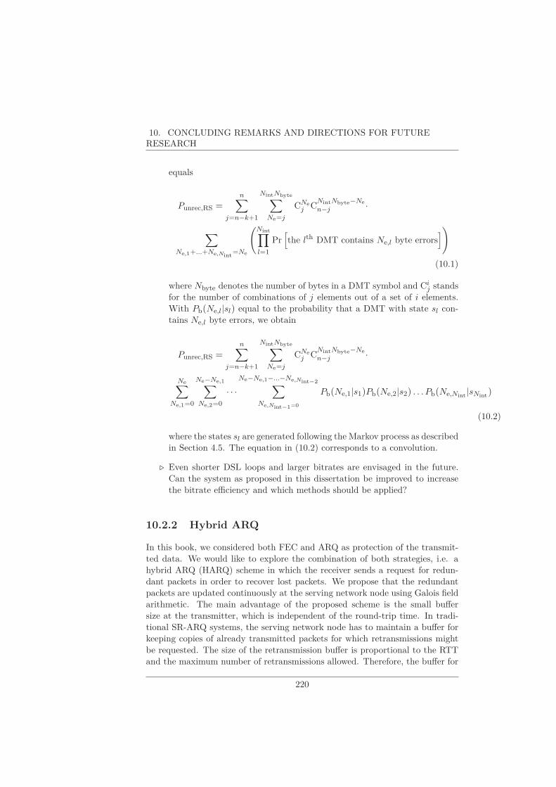
10. CONCLUDING REMARKS AND DIRECTIONS FOR FUTURERESEARCH
equals
Punrec,RS =n∑
j=n−k+1
NintNbyte∑
Ne=j
CNej C
NintNbyte−Ne
n−j ·
∑
Ne,1+...+Ne,Nint=Ne
(Nint∏
l=1
Pr[
the lth DMT contains Ne,l byte errors])
(10.1)
where Nbyte denotes the number of bytes in a DMT symbol and Cij stands
for the number of combinations of j elements out of a set of i elements.With Pb(Ne,l|sl) equal to the probability that a DMT with state sl con-tains Ne,l byte errors, we obtain
Punrec,RS =n∑
j=n−k+1
NintNbyte∑
Ne=j
CNej C
NintNbyte−Ne
n−j ·
Ne∑
Ne,1=0
Ne−Ne,1∑
Ne,2=0
· · ·Ne−Ne,1−...−Ne,Nint−2∑
Ne,Nint−1=0
Pb(Ne,1|s1)Pb(Ne,2|s2) . . . Pb(Ne,Nint|sNint
)
(10.2)
where the states sl are generated following the Markov process as describedin Section 4.5. The equation in (10.2) corresponds to a convolution.
⊲ Even shorter DSL loops and larger bitrates are envisaged in the future.Can the system as proposed in this dissertation be improved to increasethe bitrate efficiency and which methods should be applied?
10.2.2 Hybrid ARQ
In this book, we considered both FEC and ARQ as protection of the transmit-
ted data. We would like to explore the combination of both strategies, i.e. a
hybrid ARQ (HARQ) scheme in which the receiver sends a request for redun-
dant packets in order to recover lost packets. We propose that the redundant
packets are updated continuously at the serving network node using Galois field
arithmetic. The main advantage of the proposed scheme is the small buffer
size at the transmitter, which is independent of the round-trip time. In tradi-
tional SR-ARQ systems, the serving network node has to maintain a buffer for
keeping copies of already transmitted packets for which retransmissions might
be requested. The size of the retransmission buffer is proportional to the RTT
and the maximum number of retransmissions allowed. Therefore, the buffer for
220

10.2. FUTURE WORK
HARQ can be designed to be much smaller than for SR-ARQ. This advantageis particular important in the context of streaming on-demand video services,where the buffer size is proportional to the number of users served by the con-sidered node (say 1000). In spite of the availability of Terabyte hard disks, onsome devices and in some systems is the memory capacity still limited.
It has been shown in Chapter 2 that FEC introduces an overhead bit ratethat is (up to several orders of magnitude) larger than that of ARQ. Indeed,FEC adds a fixed number of redundant packets to each block of informationpackets, whereas ARQ retransmits only when packets are actually lost. Here, weintroduce a HARQ scheme that operates from a network node and only requestsa retransmit when a packet is actually lost (thus having a similar overhead bitrate as ARQ, much smaller than the one of traditional FEC).
10.2.2.1 Description of the HARQ Scheme
At the transmission instant of the kth information packet D(k), the servingnode computes on the fly L redundant packets S1(k), . . . ,SL(k), that mightbe requested by the user in order to recover lost information packets. We as-sume that a packet contains J log2(NHARQ) bits. The redundant packets arerepresented by row vectors containing J elements from GF(NHARQ), and arecomputed recursively as
Sl(k) = D(k) + αl−1Sl(k − 1) for l = 1, . . . ,L (10.3)
where α denotes a primitive element of GF(NHARQ), which satisfies αNHARQ−1 =1. The L redundant packets contained in S(k) are stored at the serving networknode during the inter-packet interval between the transmission instants of D(k)and D(k + 1), requiring a buffer size of L packets. When requested by the user,redundant packets from S(k) are transmitted between the information packetsD(k) and D(k + 1). The information packets and the redundant packets alsocontain their sequence number, to allow identification by the user.
Our HARQ scheme is based on the fact that, under certain conditions, know-ing at the user side the first L′ (≤ L) rows of the state matrix at instants k
and k + m allows to recover up to L′ lost information packets from the set{D(k + 1), . . . ,D(k + m)} of transmitted information packets.
A loss period starts at k = k0 when the user knows the state matrix S(k0 −1)but packet D(k0) is lost, and ends when sufficient redundant information hasbeen received to recover the state matrix for the first time since the loss of
D(k0). When the number of lost information packets during the current lossperiod reaches L+ 1, the set of lost information packets cannot be recovered. In
this case, the user waits for the serving network node’s response to the request
for the entire state matrix (i.e., all L rows), that has been issued when the Lth
information packet loss occurred. When this response is affected by packet loss,
221

10. CONCLUDING REMARKS AND DIRECTIONS FOR FUTURERESEARCH
the user persistently requests for the entire state matrix until it is correctlyreceived. The current loss period, which is referred to as an unrecoverable lossperiod, ends upon the correct reception of the entire state matrix.
A simplified analysis gets us the probability of an unrecoverable loss periodwith L + 1 information packet erasures, denoted as Punrec,ARQ,
Punrec,HARQ =Pe,p(1− (1− Pe,p)r)L
L∏
i=1(1− (1− Pe,p)rPi)
≈ rLP L+1e,p (10.4)
with Pe,p denoting the packet loss probability in downstream directions, r equalsthe number of packets transmitted during the RTT, and Pi is the probabilitythat a request for i state vectors does not give rise to a correctly receivedresponse given by
Pi = 1− (1− Pe,p)i ≈ iPe,p (10.5)
where we assume that the erasure probability of a request message is negligibleas compared to Pe,p. The resulting average transmission overhead amounts toE[ovh] ≈ Pe,p.
The probability of an unrecoverable packet and the overhead for SR-ARQ isgiven by (2.16) and (2.18), respectively, where Pe,DTU must be substituted byPe,p.
We present some numerical results for this simplified analysis in Figures10.1-10.3 for r = 30:
• Figure 10.1 shows Punrec,HARQ from (10.4) along with its asymptote forsmall Punrec,HARQ, as a function of Pe,p, for L = 2, 4, 6. Also shown isPunrec,HARQ = Pe,p, which corresponds to the case where no attempt ismade to recover lost packets. We observe that Punrec,HARQ converges toits asymptote (10.4) for small Pe,p, and to Pe,p for large Pe,p.
• Figure 10.2 displays Punrec for HARQ with L = 4 and r = 30, and for SR-ARQ with Nretr = 1, 2, 3. We observe that a minimum value of Nretr = 2
(corresponding to a retransmit buffer of 60 packets) is required in orderto beat the performance of HARQ in the region that is visible.
• Figure 10.3 shows the average downstream transmission overhead E[ovh]for HARQ with L = 4 and r = 30 and for SR-ARQ with Nretr = 1, 2, 3,along with the low-Pe,p asymptote E[ovh] = Pe,p. We observe that forvalues of small Pe,p, the actual overhead is very small, and close to Pe,pfor all systems.
222

10.2. FUTURE WORK
10�4
10�3
10�2
10�1
100
10�8
10�6
10�4
10�2
100
Pe,p
Punre
c,H
AR
Q
L = 2
L = 2, asymptote
L = 4
L = 4, asymptote
L = 6
L = 6, asymptote
Pe,p
Figure 10.1: Punrec,HARQ as a function of Pe,p, for r = 30 and L = 2, 4, 6.
10�4
10�3
10�2
10�1
100
10�8
10�6
10�4
10�2
100
Pe,p
Punre
c
L = 4
L = 4, approximation
Nretr
= 1
Nretr
= 2
Nretr
= 3
Figure 10.2: Punrec,HARQ for HARQ with L = 4 and r = 30, and for SR-ARQ
with Nretr = 1, 2, 3.
223
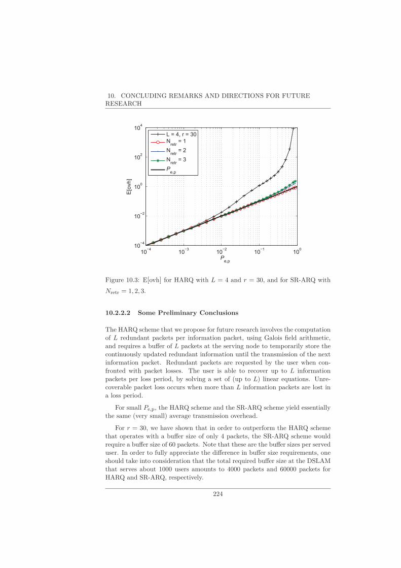
10. CONCLUDING REMARKS AND DIRECTIONS FOR FUTURERESEARCH
10�4
10�3
10�2
10�1
100
10�4
10�2
100
102
104
Pe,p
E[o
vh]
L = 4, r = 30
Nretr
= 1
Nretr
= 2
Nretr
= 3
Pe,p
Figure 10.3: E[ovh] for HARQ with L = 4 and r = 30, and for SR-ARQ with
Nretr = 1, 2, 3.
10.2.2.2 Some Preliminary Conclusions
The HARQ scheme that we propose for future research involves the computationof L redundant packets per information packet, using Galois field arithmetic,and requires a buffer of L packets at the serving node to temporarily store thecontinuously updated redundant information until the transmission of the nextinformation packet. Redundant packets are requested by the user when con-fronted with packet losses. The user is able to recover up to L informationpackets per loss period, by solving a set of (up to L) linear equations. Unre-coverable packet loss occurs when more than L information packets are lost ina loss period.
For small Pe,p, the HARQ scheme and the SR-ARQ scheme yield essentiallythe same (very small) average transmission overhead.
For r = 30, we have shown that in order to outperform the HARQ schemethat operates with a buffer size of only 4 packets, the SR-ARQ scheme wouldrequire a buffer size of 60 packets. Note that these are the buffer sizes per serveduser. In order to fully appreciate the difference in buffer size requirements, oneshould take into consideration that the total required buffer size at the DSLAMthat serves about 1000 users amounts to 4000 packets and 60000 packets forHARQ and SR-ARQ, respectively.
224

10.2. FUTURE WORK
The presented HARQ scheme is more computationally demanding than SR-ARQ, mainly because of the computation of recursions (10.3) at the serving nodeand at the user side, respectively. A detailed examination of the complexitycomparison should be performed.
Another point of attention is the singularity of the set of linear equationsin (10.3), that needs to be solved to recover possible lost packets, and how toovercome this possible singularity.
Also, the HARQ scheme can be expanded by including a timer at the userside, in order to limit the latency of the packet recovery process. This is mo-tivated by the observation that it makes no sense to recover packets that areanyway to late to be delivered to the play-out buffer of the video application.
10.2.3 Other Correcting Codes
A first attempt to tackle the investigation of other codes is made in [91] wherewe compare RS codes with the popular Raptor codes. Raptor codes [92] havesignificantly lower decoding complexity than Reed-Solomon codes. The successof Raptor codes is witnessed by their adoption in the recent multimedia commu-nication standards such as 3GPP MBMS (Multimedia Broadcast/MultimediaService) [93] and DVB-H [94]. We want to compare the RS codes with theRaptor codes in terms of performance and decoding complexity.
10.2.3.1 RS Erasure Coding
In the sequel, a (video) information packet refers to video payload of the IPpacket, and contains L bits. Per group of k of these video information packets,an additional n − k parity packets are transmitted. This results in a systematicpacket codeword of n packets. The parity packets are constructed such thattaking from each packet the ith block of q bits yields an RS(n,k) codeword, for alli = 1, 2, . . . ,L/q. This construction is illustrated in Figure 10.4. Hence, when e
packets from the packet codeword are erased, each of the L/q RS codewords isaffected by exactly e symbol erasures. The code parameters n and k should beselected such that the overhead and latency are limited to reasonable values.
In [91], an efficient erasure decoding algorithm is presented based on [27].
The resulting decoding complexity of a RS packet codeword is dominated by
4 · 2q q L additions in Z and 2q q L multiplications in Z, with L the number
of bits in a video packet. Note that the decoding complexity of the shortened
RS(n,k) code is determined by the size 2q of the Galois field, rather than the
specific code parameters n and k.
225

10. CONCLUDING REMARKS AND DIRECTIONS FOR FUTURERESEARCH
1 symbol = q bits
�
�
�
�
�
�
�
�
�
k video
information
packets
RS codeword
n-k parity
packets
Figure 10.4: Construction of a packet codeword of the RS(n,k) code.
10.2.3.2 Raptor Codes
The Raptor (n,k) codes are non-systematic binary codes. Raptor codes arerateless, which means that for a given information word a potentially infinitenumber of code bits can be produced. Raptor codes are designed such that ahigh probability of decoding occurs when n = k(1+ ǫ) code bits are received,where k is the number of information bits and the overhead parameter ǫ is adesign parameter of the Raptor code.
The construction of a Raptor packet codeword is illustrated in Figure 10.5.From each group of k video information packets, n code packets are computed.The sequence of each ith bit of all code packets forms the Raptor codewordcorresponding to the information word that contains each ith bit of all videoinformation packets, for all i = 1, 2, . . . ,L. The latency introduced by theRaptor code equals the duration of the packet codeword.
Raptor codes [92] are built on LT codes by first applying a pre-code to theinformation bits, followed by an LT code operating on the pre-code output bits.As pre-code, we use an irregular LDPC code. The LT codes were invented byLuby [95]. Each packet in the codeword is obtained from a bitwise exclusive-or(XOR) of a uniformly random selection of d information packets, where d is thedegree of the code packet, and d is specified by a suitable degree distribution,called the weakened LT (wLT) distribution [92].
The LT decoding is achieved using the belief propagation algorithm on abipartite graph that represents the information packets and the coded packets;
226

10.2. FUTURE WORK
1 symbol
= 1 bit
�
�
�
�
�
�
�
�
�
n code
packets
Fountain
codeword
Figure 10.5: Construction of a packet codeword of the Raptor code on the
application layer.
each coded packet is connected to the information packets that contribute to theconsidered coded packet. First, all code packets with degree one are identified.The corresponding information packets are trivially resolved, and the degree ofall neighbours in the graph of the resolved information packets is reduced byone. This allows to resolve the information packets that are connected to codedpackets with original degree of two. This process is repeated until all infor-mation packets have been resolved (successful decoding) or only code packetswith degree higher than one remain (decoding fails). As this decoding processrequires only XOR operations, the decoding complexity for LT codes is muchsmaller than for RS codes.
The total overhead of the Raptor codes, ǫ depends on the overheads of thetwo encoding blocks (pre-code and wLT code):
(1+ ǫ) = (1+ ǫLDPC)(1+ ǫwLT) (10.6)
In [92] it has been suggested to set ǫwLT = ǫ/2.
Decoding of the Raptor code is done in two steps. First, the LT decoderoperates on the received packet codeword and returns a number of packets thathave been generated by the LDPC encoder. Then the LDPC decoder attemps torecover the information packets, making use of the LT decoder output. In [91],we derive that the decoding complexity of the LT part is given by k(1+ ǫ)(E[d]−1) XOR operations on packets. LDPC decoding can use the same simplified
227

10. CONCLUDING REMARKS AND DIRECTIONS FOR FUTURERESEARCH
102
103
104
104
106
108
1010
1012
k
com
ple
xity
RS
Raptoroverhead = 20%
Figure 10.6: Comparison of the decoding complexity of the RS and Raptor
codes.
belief propagation algorithm on a Tanner graph that represents the LDPC code.The corresponding decoding complexity equals k(1+ ǫLDPC)(E[ld] − 1) XORoperations on packets, with E[ld] the average left degree in the Tanner graph.
10.2.3.3 Some Numerical Results
Considering an IP packet of L = 104 bits, we have displayed in Figure 10.6, thedecoding complexity of a packet codeword when using the RS or Raptor code,as a function of the number k of information packets in a packet codeword. Thetotal transmission overhead is equal to 20%. Assuming a 64-bit processor, oneunit of complexity corresponds to one addition in Z, one multiplication in Z
or 64 XOR operations. The curves confirm the higher decoding complexity ofthe RS code. The curve of the RS code increases step-by-step, as the decodingcomplexity is a function of the size 2q of the GF; we restrict our attention tovalues of q that are multiples of 8. A RS code with q = 8 (for which themaximum value of k is 212 when considering a 20% overhead) has the samedecoding complexity as a Raptor code with k = 89105 information packets. Itis clear that for the same decoding complexity, the Raptor codes are allowed tobe much longer than the RS codes.
In Figure 10.7 we show the simulated decoder performance of the Raptor
228

10.2. FUTURE WORK
0 0.05 0.1 0.15 0.2 0.25 0.3
10 4
10 3
10 2
10 1
100
ovh
Punrec
Raptor,!k!=!7300
Figure 10.7: Performance of the Raptor code as a function of the overhead in
the absence of erasures.
code as a function of the overhead, under the assumption that none of thepackets of the packet codeword has been erased. In this case, the simplifieddecoding might fail because of the random nature of the code (e.g., for someof the coded packets, the LT decoder cannot reduce their degree to 1). Forthe Raptor code we have selected k = 7300 which results in a latency of 10seconds (with L = 104 bits and a video bit rate Rvideo = 7.3 Mbit/s), whichis acceptable for streaming video-on-demand applications. As pre-code of theRaptor code, we use a right-Poisson, left-regular LDPC code, with left degreeequal to 4 [92].
In Figure 10.8, we compare the different codes in the context of streamingon-demand video. We take Rvideo = 7.3 Mbit/s, L = 104 and allow a trans-mission overhead of 20%. We limit the latency to a maximum of 10 seconds,which corresponds to Raptor codewords of maximum 7300 video informationpackets. We consider Raptor codes designed for respectively ǫ = 0.05, ǫ = 0.1,ǫ = 0.15 and ǫ = 0.2 but transmit a higher overhead equal to 20%, which ispossible due to the rateless nature of the code. For the RS code, we select thecode with n = 254 and k = 212. Our performance target is to achieve an av-erage of no more than 1 decoding error in 4 hours. For a given decoding errorprobability Punrec, the average number of decoding errors in 4 hours is given by4 · 3600RvideoPunrec/(kL) ≈ 107Punrec/k. In the absence of error control, the
229

10. CONCLUDING REMARKS AND DIRECTIONS FOR FUTURERESEARCH
10�2
10�1
100
10�1
100
101
102
103
104
Pe,p
E[#
decodin
g e
rrors
in 4
hr]
RS, k = 212
Raptor, k = 7300, ε = 5%
Raptor, k = 7300, ε = 10%
Raptor, k = 7300, ε = 15%
Raptor, k = 7300, ε = 20%
overhead = 20%
Figure 10.8: E[# decoding errors in 4 hr] for the Raptor and RS code.
erasure probability Pe,p should be limited to about 10−7 in order to achieve onaverage not more than 1 erasure in 4 hours. Figure 10.8, shows the performanceof the Raptor codes and the RS code as a function of the erasure probabilityPe,p at the input of the decoder. The RS code and the Raptor code designedfor ǫ = 0.05 have similar performance and outperform the other Raptor codes.These two codes achieve the performance target for Pe,p < 9× 10⁻². The Rap-tor code designed for ǫ = 0.2 has the lowest performance. The price to payfor the RS code is its decoding complexity, which is larger than for the Raptorcodes by a factor of about 12.
10.2.3.4 Some Conclusions
It is clear that depending on the requirements of the system, e.g., a low decodingcomplexity, low memory requirements, low latency constraints,... other codesor ARQ protocols will satisfy our needs with similar error performance. In thecomparison of examination in this section, the Raptor code designed for ǫ = 0.05
performs as good as the RS code, at the gain of a 10 times smaller decodingcomplexity.
Further research might look into the effect of the arguments and degreedistribution of the Raptor code in more detail and explore the combination ofLT codes with other LDPC codes, e.g., the regular LDPC codes as used in PartI of this book.
230

10.3. PUBLICATIONS
10.3 Publications
Our work, of which was largely reported in this dissertation, has been presentedin the following refereed journal and conference publications:
Journal Publications
• EURASIP Journal on Advances in Signal Processing: [59]
• IEEE Journal on Selected Areas in Communications: [96]
Conference Publications
• IEEE Symposium on Communications and Vehicular Technology in theBenelux: [97]
• NewCOM++ ACoRN Joint Workshop: [98]
• IEEE International Symposium on Information Theory and Its Applica-tions (ISITA): [91]
• IEEE International Conference on Communications (ICC): [99,100]
231

10. CONCLUDING REMARKS AND DIRECTIONS FOR FUTURERESEARCH
232

Bibliography
[1] (2015) Cisco visual networking index: Forecast andmethodology, 2014-2019 white paper. [Online]. Available:http://www.cisco.com/c/en/us/solutions/collateral/service-provider/ip-ngn-ip-next-generation-network/white_paper_c11-481360.pdf
[2] G. Ungerboeck and I. Csajka, “On improving data-link performance by in-creasing the channel alphabet and introducing sequence coding,” in Proc.
IEEE International Symposium on Information Theory, Jun. 1976, p. 53.
[3] G. Ungerboeck, “Channel coding with multilevel/phase signals,” IEEE
Transactions on Information Theory, vol. 28, pp. 55–67, Jan. 1982.
[4] “ITU-T Recommendation G.992.1: Single-pair high-speed digital sub-scriber line (SHDSL) transceivers.”
[5] “ITU-T Recommendation G.993.2: Very high speed digital subscriber linetransceivers 2 (VDSL2).”
233

BIBLIOGRAPHY
[6] P. Elias, “Coding for noisy channels,” IRE Convention Record, vol. 3, part4, pp. 37 – 46, 1955.
[7] A. J. Viterbi, “Error bounds for convolutional codes and an asymptoti-cally optimum decoding algorithm,” IEEE Transactions on Information
Theory, vol. 13, no. 2, pp. 260 – 269, Apr. 1967.
[8] C. E. Shannon, “A mathematical theory of communication,” The Bell
System Technical Journal, vol. 27, pp. 379–423, Jul. 1948.
[9] R. G. Gallager, Low Density Parity Check Codes. MA: MIT Press, 1963.
[10] D. J. C. MacKay and R. M. Neal, “Near Shannon limit performance of lowdensity parity check codes,” IEEE Transactions on Information Theory,vol. 32, pp. 1646 – 1646, Aug. 1996.
[11] D. J. C. MacKay, “Good error-correcting codes based on very sparse ma-trices,” Electronics Letters, vol. 45, pp. 399 – 431, Mar. 1999.
[12] M. Fossorier, M. Mihaljevic, and H. Imai, “Reduced complexity iterativedecoding of low-density parity check codes based on belief propagation,”IEEE Transactions on Communications, vol. 47, pp. 673 – 680, May 1999.
[13] A. Emran and M. Elsabrouty, “Simplified variable-scaled min sum LDPCdecoder for irregular LDPC codes,” in Proc. IEEE Consumer Communi-
cations and Networking Conference (CCNC), Jan. 2014, pp. 518 – 523.
[14] S. ten Brink, G. Kramer, and A. Ashikhmin, “Design of low-density parity-check codes for modulation and detection,” IEEE Transactions on Com-
munications, vol. 52, pp. 670 – 678, Apr. 2004.
[15] M. Ardakani and F. R. Kschischang, “A more accurate one-dimensionalanalysis and design of irregular LDPC codes,” IEEE Transactions on
Communications, vol. 52, pp. 2106 – 2114, Dec. 2004.
[16] T. J. Richardson and R. L. Urbanke, “The capacity of low-density parity-check codes under message-passing decoding,” IEEE Transactions on In-
formation Theory, vol. 47, pp. 619 – 637, Feb. 2001.
[17] S. M. Alamouti, “A simple transmit diversity technique for wirelesscommunications,” IEEE Journal on Selected Areas in Communications,vol. 16, no. 8, pp. 1451–1458, October 1998.
[18] E. Biglieri, R. Calderbank, A. Constantinides, A. Goldsmith, A. Paulraj,and H. V. Poor, “MIMO wireless communications,” Cambridge University
Press, 2007.
234

BIBLIOGRAPHY
[19] V. Tarokh, N. Seshadri, and A. R. Calderbank, “Space-time codes forhigh data rate wireless communication: performance criterion and codeconstruction,” IEEE Transactions on Information Theory, vol. 44, no. 2,pp. 744–765, March 1998.
[20] J. Proakis, Digital Communications. McGraw Hill, 2000.
[21] I. S. J. Reed and G. Solomon, “Polynomial codes over certain finite fields,”Journal of the Society for Industrial and Applied Mathematics, vol. 8,no. 2, pp. 300 – 304, Jun. 1960.
[22] G. C. Clark Jr. and J. B. Cain, Error-Correction Coding for Digital Com-
munications. Springer, 1981.
[23] S. B. Wicker and V. K. Bhargava, Reed-Solomon codes and their Applica-
tions. IEEE Press, 1994.
[24] Y. M. Sugiyama, S. H. Kasahara, and T. Namekawa, “A method forsolving the key equation for decoding of Goppa codes,” Information and
Control, vol. 27, pp. 87 – 89, Jan. 1975.
[25] R. E. Blahut, Theory and practice of error control codes. Reading, Mass.:Addison Wesley, 1984.
[26] G. D. J. Forney, “On decoding BCH codes,” IEEE Transactions on Infor-
mation Theory, vol. IT-11, pp. 393 – 403, Oct. 1965.
[27] F. Didier, “Efficient erasure decoding of Reed-Solomon codes,” 2009.[Online]. Available: arXiv:0901.1886
[28] T. Starr, J. M. Cioffi, and P. J. Silverman, Understanding Digital Sub-
scriber Line Technology. Prentice Hall, 1999.
[29] P. Golden, H. Dedieu, and K. Jacobsen, Fundamentals of DSL technology.
Auerbach Publications, 2006.
[30] V. Oksman, H. Schenk, A. Clausen, J. Cioffi, M. Mohseni, G. Ginis,
C. Nuzman, J. Maes, M. Peeters, K. Fisher, and P.-E. Eriksson, “The
ITU-T’s new G.vector standard proliferates 100 Mb/s DSL,” IEEE Com-
munications Magazine, vol. 48, no. 10, pp. 140 – 148, Oct. 2010.
[31] M. Guenach, J. Maes, M. Timmers, O. Lamparter, J.-C. Bisschoff, and
M. Peeters, “Vectoring in DSL systems: practices and challenges,” in Proc.
IEEE Global Telecommunications Conference (GLOBECOM),, Houston,
Texas, Dec. 2011.
[32] R. Essiambre, G. Kramer, P. Winzer, G. Foschini, and B. Goebel, “Ca-
pacity limits of optical fiber networks,” Journal of Lightwave Technology,
vol. 28, pp. 662–701, Feb. 2010.
235

BIBLIOGRAPHY
[33] P. Ödling, T. Magesacher, S. Host, P. Borjesson, M. Berg, and E. Areizaga,“The fourth generation broadband concept,” IEEE Communications Mag-
azine, vol. 47, no. 1, pp. 62 – 69, Jan. 2009.
[34] M. Timmers, M. Guenach, C. Nuzman, and J. Maes, “G.fast: evolving thecopper access network,” IEEE Communications Magazine, vol. 51, no. 8,pp. 74 – 79, Aug. 2013.
[35] I. Almeida, A. Klautau, and C. Lu, “Capacity analysis of G.fast systemsvia time-domain simulations,” in Proc. IEEE International Conference on
Communications (ICC), Budapest, Hungary, Jun. 2013.
[36] G. Ginis and J. M. Cioffi, “Vectored transmission for digital subscriber linesystems,” IEEE Journal on Selected Areas in Communications, vol. 20,
no. 5, pp. 1085 – 1104, Jun. 2002.
[37] R. Cendrillon, G. Ginis, E. Van den Bogaert, and M. Moonen, “A near-
optimal linear crosstalk precoder for downstream VDSL,” IEEE Transac-
tions on Communications, vol. 55, no. 5, pp. 860 – 863, May 2007.
[38] R. Strobel, R. Stolle, and W. Utschick, “Wideband modeling of twisted-
pair cables for MIMO applications,” in Proc. IEEE Global Telecommuni-
cations Conference (GLOBECOM),, Dec. 2013, pp. 2828 – 2833.
[39] R. Kirkby, “Text for ’Realistic Impulsive Noise Model’,” ETSI TM6
011T20, Feb. 2001.
[40] I. Mann, S. McLaughlin, W. Henkel, R. Kirby, and T. Kessler, “Impulse
noise generation with appropriate amplitude, length, inter-arrival, and
spectral characteristics,” IEEE Journal on Selected Areas in Communica-
tions, vol. 20, no. 5, pp. 901–912, Jun. 2002.
[41] D. Zhang, K. Ho-Van Khuong, and T. Le-Ngoc, “Impulse noise detec-
tion techniques for retransmission to reduce delay in DSL systems,” in
Proc. IEEE International Conference on Communications (ICC), Ottawa,
Canada, Jun. 2012.
[42] “ITU-T Recommendation G.9701: Fast access to subscriber terminals
(G.fast) - Physical layer specification.”
[43] H. A. Suraweera, C. Chai, S. J., and A. J., ““analysis of impulse noise
mitigation techniques for digital television systems,” in Proc. 8th Interna-
tional OFDM Workshop, Hamburg, Sep. 2003, pp. 172 – 176.
[44] A. J., M. Feramez, and H. A. Suraweera, “Optimum noise thresholds
in decision directed impulse noise mitigation for OFDM,” in Proc. In-
ternational Symposium on Communication Systems Networks and Digital
Signal Processing (CSNDSP 2004), Newcastle upon Tyne, UK, Jul. 2004,
pp. 168 – 171.
236

BIBLIOGRAPHY
[45] A. J. and H. A. Suraweera, “Impulse noise mitigation for OFDM usingdecision directed noise estimation,” in Proc. IEEE International Sympo-
sium on Spread Spectrum Techniques and Applications (ISSSTA 2004),Sydney, Australia, Aug. 2004, pp. 174 – 178.
[46] D. Fertonami and G. Colavolpe, “On reliable communications over chan-nels impaired by bursty impulse noise,” IEEE Transactions on Commu-
nications, vol. 57, pp. 2024 – 2030, Jul. 2009.
[47] J. Mitra and L. Lampe, “Convolutionally coded transmission over markov-gaussian channels: analysis and decoding metrics,” IEEE Transactions on
Communications, vol. 58, pp. 1939 – 1949, Jul. 2010.
[48] J. Smith, “Odd-bit quadrature amplitude-shift keying,” IEEE Transac-
tions on Communications, vol. 23, pp. 385 – 389, Mar. 1975.
[49] P. K. Vitthaladevuni, “Exact ber computation for cross QAM constella-tions,” IEEE Transactions on Wireless Communications, vol. 4, pp. 3039– 3050, Nov. 2005.
[50] L.-F. Wei, “Trellis-coded modulation with multidimensional constella-tions,” IEEE Transactions on Information Theory, vol. 33, pp. 483–501,Jul. 1987.
[51] “ITU-T Recommendation G.9960: Unified high-speed wireline-basedhome networking transceivers – system architecture and physical layerspecification.”
[52] Y. Li and W. E. Ryan, “Mutual-information-based adaptive bit-loading al-gorithms for LDPC-coded OFDM,” IEEE Transactions on Wireless Com-
munications, vol. 6, pp. 1670 – 1680, May 2007.
[53] J. Maes, P. Spruyt, and S. Vanhastel. (2014, Jul.) G.fast breaksthrough the gigabit barrier. TechZine Alcatel-Lucent. [Online]. Available:http://www2.alcatel-lucent.com/techzine/g-fast-breaks-gigabit-barrier/
[54] D. Z. Filho, R. R. Lopes, R. Ferrari, and R. Suyama, “Bit loading for pre-coded DSL systems,” in Proc. IEEE International Conference on Acous-
tics, Speech and Signal Processing (ICASSP), vol. 3, 2007, pp. 353–356.
[55] J. Maes and C. Nuzman, “Energy efficient discontinuous operation in vec-tored G.fast,” in Proc. IEEE International Conference on Communica-
tions (ICC), Sydney, Australia, Jun. 2014.
[56] G. D. J. Forney and G. Ungerboeck, “Modulation and coding for linear
gaussian channels,” IEEE Transactions on Information Theory, vol. 44,
no. 6, pp. 2384 – 2415, Oct. 1998.
237
BIBLIOGRAPHY
[57] J. Bingham, “Multicarrier modulation for data transmission: an ideawhose time has come,” IEEE Communications Magazine, vol. 28, pp.5–14, May 1990.
[58] H. Liu and G. Li, OFDM-Based Broadband Wireless Networks: Design
and Optimization. Wiley-Blackwell, 2005.
[59] J. Neckebroek, F. Vanhaverbeke, D. De Vleeschauwer, and M. Moeneclaey,“Protection of video packets over a wireless Rayleigh fading link: FECversus ARQ,” EURASIP Journal on Advances in Signal Processing, 2008,article ID 852697.
[60] F. Vanhaverbeke, F. Simoens, M. Moeneclaey, and D. De Vleeschauwer,“Binary erasure codes for packet transmission subject to correlated era-sures,” in 2006 Pacific-Rim Conference on Multimedia, Hangzhou, China,Nov. 2006, pp. 48–55.
[61] N. Degrande, K. Laevens, D. De Vleeschauwer, and R. Sharpe, “Increas-ing the user perceived quality for IPTV services,” IEEE Communications
Magazine, vol. 46, no. 2, pp. 94–100, February 2008.
[62] G. Liang and B. Liang, “Balancing interruption frequency and bufferingpenalties in VBR video streaming,” Proc. IEEE International Conference
on Computer Communications (INFOCOM 2007), pp. 1406–1414, May2007, Anchorage, USA.
[63] T. Stockhammer, H. Jenkac, and G. Kuhn, “Streaming video over vari-able bit-rate wireless channels,” IEEE Transactions on Multimedia, vol. 6,no. 2, pp. 268–277, April 2002.
[64] F. Borgonovo and A. Capone, “Efficiency of error-control schemes for real-time wireless applications on the Gilbert channel,” IEEE Transactions on
Vehicular Technology, vol. 54, no. 1, pp. 246–258, January 2005.
[65] M. Tun, K. K. Loo, and J. Cosmas, “Error-resilent performance of Dirac
video codec over packet-erasure channel,” IEEE Transactions on Broad-
casting, vol. 53, no. 3, pp. 649–659, September 2007.
[66] S. W. Kim, S. Y. Kim, S. Kim, and J. Heo, “Performance analysis of
forward error correcting codes in IPTV,” IEEE Transactions on Consumer
Electronics, vol. 54, no. 2, pp. 376–380, May 2008.
[67] M. Luby, T. Stockhammer, and M. Watson, “Application layer FEC in
IPTV services,” IEEE Communications Magazine, vol. 46, no. 5, pp. 94–
101, May 2008.
[68] C.-Y. Hsu, A. Ortega, and M. Khansari, “Rate control for robust video
transmission over burst-error wireless channels,” IEEE Journal on Selected
Areas in Communications, vol. 17, no. 5, pp. 756–773, May 1999.
238

BIBLIOGRAPHY
[69] J. Xu, X. Shen, J. W. Mark, and J. Cai, “Quasi-optimal channel assign-ment for real-time video in OFDM wireless systems,” IEEE Transactions
on Wireless Communications, vol. 7, no. 4, pp. 1417– 1427, April 2008.
[70] Y. Wang and Q.-F. Zhu, “Error control and concealment for video com-munication: A review,” Proc. IEEE, vol. 86, no. 5, May 1998.
[71] H. O. Burton and D. D. Sullivan, “Errors and error control,” Proc. IEEE,vol. 60, pp. 1293–1301, November 1972.
[72] R. A. Comroe and D. J. Costello Jr., “ARQ schemes for data transmissionin mobile radio systems,” IEEE Journal on Selected Areas in Communi-
cations, pp. 472–481, July 1984.
[73] H. Yang, P. Smulders, and M. Herben, “Channel characteristics andtransmission performance for various channel configurations at 60 GHz,”EURASIP journal on Wireless Communications and Networking - special
issue on millimeter-wave wireless communication systems: theory and ap-
plications, 2007, art. No 19613.
[74] M. Robin and M. Poulin, Digital Television Fundamentals. McGraw-Hill,2000.
[75] P. J. Smith, M. Shafi, and H. Gao, “Quick simulation: A review of impor-tance sampling techniques in communication systems,” IEEE Journal on
Selected Areas in Communications, vol. 15, pp. 597–613, May 1997.
[76] R. Srinivasan, Importance Sampling: Applications in Communications and
Detection. Springer, 2002.
[77] M. H. Kalos and P. A. Whitlock, Monte Carlo Methods. J. Wiley, 2008.
[78] “ITU-T Recommendation G.995.1: Overview of digital subscriber line(DSL) recommendations.”
[79] B. G. Haskell, A. Puri, and A. N. Netravali, Digital Video: an Introduction
to MPEG-2. Springer, 1996.
[80] P. D. Symes, Digital Video Compression. McGraw-Hill, 2003.
[81] J. Greengrass, J. Evans, and A. C. Begen, “Not all packets are equal,part 1: Streaming video coding and SLA requirements,” IEEE Internet
Computing, vol. 13, pp. 70–75, January-February 2009.
[82] ——, “Not all packets are equal, part 2: The impact of network packetloss on video quality,” IEEE Internet Computing, vol. 13, pp. 74 – 82,March-April 2009.
239

BIBLIOGRAPHY
[83] S. Kanumuri, P. C. Cosman, A. R. Reibman, and V. A. Vaishampayan,“Modeling packet-loss visibility in MPEG-2 video,” IEEE Transactions
on Multimedia, vol. 8, no. 2, pp. 341–355, 2006.
[84] J. Zhang, J. F. Arnold, and M. R. Frater, “A cell-loss concealment tech-nique for MPEG-2 coded video,” IEEE Transactions on Circuits and Sys-
tems for Video Technology, vol. 10, no. 4, pp. 659–665, June 2000.
[85] T. Wiegand, G. J. Sullivan, G. Bjontegaard, and A. Luthra, “Overview ofthe H.264/AVC video coding standard,” IEEE Transactions on Circuits
and Systems for Video Technology, vol. 13, no. 7, pp. 560–576, July 2003.
[86] A. R. Reibman and D. Poole, “Characterizing packet-loss impairments incompressed video,” Proc. IEEE International Conference on Image Pro-
cessing ICIP2007, pp. 77–80, September 2007, San Antonio, USA.
[87] “Technical report TR-126, triple-play services quality of experience(QoE) requirements,” DSL Forum, Tech. Rep., December 2006,http://www.broadband-forum.org/technical/download/TR-126.pdf.
[88] A. Gurtov and S. Floyd, “Modelling wireless links for transport protocols,”ACM Computer Communications Review, vol. 34, no. 2, pp. 85–96, April2004.
[89] C. Hoene and A. Wolisz, “Measuring the impact of slow user motion onpacket loss and delay over IEEE 802.11b wireless links,” Proceedings of the
28th Annual IEEE International Conference on Local Computer Networks
(LCN ’03), pp. 652–662, October 2003, Bonn, Germany.
[90] T. A. Wysocki and H.-J. Zepernick, “Characterization of the indoor radiopropagation channel at 2.4 GHz,” Journal of Telecommunications and
Information Technology, vol. 1, no. 3-4, pp. 84–90, 2000.
[91] J. Neckebroek, M. Moeneclaey, and E. Magli, “Comparison of Reed-Solomon and Raptor codes for the protection of video on-demand on theerasure channel,” in Proc. IEEE International Symposium on Information
Theory and Its Applications (ISITA), Taichung, Taiwan, Oct. 2010.
[92] A. Shokrollahi, “Raptor codes,” IEEE Transactions on Information The-
ory, vol. 52, no. 6, pp. 2551–2567, June 2006.
[93] 3GPP TS 26346 v.6.2.0, Multimedia Broadcast/Multicast Service(MBMS); Protocols and codecs, September 2009. [Online]. Available:http://www.3gpp.org/ftp/Specs/html-info/26346.htm
[94] ETSI EN 302 304 V1.1.1, Digital Video Broadcasting (DVB), November2004, transmission System for Handheld Terminals (DVB-H).
240
BIBLIOGRAPHY
[95] M. Luby, “LT codes,” in Proc. of IEEE Symposium on Foundations of
Computer Science, Vancouver, Canada, November 2002, pp. 271–280.
[96] J. Neckebroek, H. Bruneel, and M. Moeneclaey, “Application layer ARQfor protecting video packets over an indoor MIMO-OFDM link with corre-lated block fading,” IEEE Journal on Selected Areas in Communications,pp. 467–475, 2010.
[97] J. Neckebroek, F. Vanhaverbeke, and M. Moeneclaey, “The impact ofRayleigh fading on packet loss in FEC-protected real-time packet-basedtransmission systems,” in Proc. IEEE Symposium on Communications
and Vehicular Technology in the Benelux (SCVT), Delft, The Netherlands,Nov. 2007.
[98] ——, “Comparison of FEC and ARQ for protection of video data overa wireless Rayleigh fading link,” in Proc. NewCOM++ - ACoRN Joint
Workshop, Barcelona, Spain, Mar. 2009.
[99] J. Neckebroek, M. Moeneclaey, M. Guenach, M. Timmers, and J. Maes,“Comparison of error-control schemes for high-rate communication overshort DSL loops affected by impulsive noise,” in Proc. IEEE International
Conference on Communications (ICC), Budapest, Hungary, Jun. 2013.
[100] J. Neckebroek, M. Moeneclaey, W. Coomans, M. Guenach, P. Tsiaflakis,R. Moraes, and J. Maes, “Novel bitloading algorithms for coded G.fastDSL transmission with linear and nonlinear precoding,” in Proc. IEEE
International Conference on Communications (ICC), London, UK, Jun.2015.
241