Fourier transforms in digital signal processing

Real space: numbers at points in time or space

How fast is the signal decaying?How fast is the signal oscillating?How many oscillators make up the signal?

Where are the particles located?What is the shape of the particles?Is this image blurred and distorted?

How does this image relate to the structure?

Real space is an intuitive representation of data

...but some questions are harder to pose

Main ideas of today’s lecture

(1) There many ways of representing numerical data

(2) Fourier space is an alternative representation based on waves of different frequency

(3) Many find Fourier space initially unintuitive

(4) Many hard problems become easier to understand and solve in Fourier space

Linear combinations

Most functions can be represented as weighted sums of other functions.

Some function of the variable x Basis functions:

a set of functions that can be combined to form other functions.

A.k.a. components, dimensions

Linear combinations

Most functions can be represented as weighted sums of other functions.

Some function of the variable x Basis functions:

a set of functions that can be combined to form other functions.

A.k.a. components, dimensionsCoefficients: how much Fi(x) is in S(x)?A.k.a. weights or coordinates

Reminder of dot product and inner product

Example:x = [ 1 4 1 ]y = [ 7 2 6 ]

dot_product(x,y) = 1*7 + 4*2 + 1*6 = 21

Orthonormal linear basis functionsOrthonormality conditionsDot product of F1 and F2 in a basis is always zero.Dot product of F1 and F1 is always one’ex. x=[1 0 0], y=[0 1 0], and z=[0 0 1]

dot_product(x,y) = 1*0 + 0*1 + 0*0 = 0dot_product(x,z) = 1*0 + 0*0 + 0*1 = 0dot_product(y,z) = 0*0 + 1*0 + 0*1 = 0dot_product(x,x) = 1*1 + 0*0 + 0*0 = 1

If basis vectors are mutually orthonormal, we can determine the coefficients for a function S simply by taking the dot product of the function and the basis functions:

ex. S = [3 2 6]wx = dot_product(S,x) = 3*1 + 2*0 + 6*0 = 3wy = dot_product(S,y) = 3*0 + 2*1 + 6*0 = 2wz = dot_product(S,z) = 3*0 + 2*0 + 6*1 = 6S = wx*x + wy*y + wz*z = [3 0 0] + [0 2 0] + [0 0 6] = [3 2 6]

Geometric interpretation:dot_product(x,y) = 0 meansarccos(x,y) = pi / 2 = 90o “a right angle between x and y”

The linear orthogonal basis for Fourier space: Waves with different frequencies

x

S(x)

Square wave function

The linear orthogonal basis for Fourier space: Waves with different frequencies

coefficients

basis functions: Wave frequency

Wave phase (offset)

x

S(x)

Square wave function

Properties of wavesWaves are represented with sine and cosine functions over time or space.

Wave frequency

Multiplying the argument of the sine function changes the frequency of the wave

Properties of waves

Sine waves can have different phases

Wave phase (offset)

ϕAdding to the argument of the sine function adds an offset

to the wave called the ‘phase’

Properties of waves

Sines and cosines are related by a 90o (π/2) phase shift

Phase shifts are less than 2π

Properties of waves

Sine waves can have different amplitudes: these will be coefficients of our combination linear combinations

Wave amplitude (scale)

Properties of waves

Polar coordinates‘Amplitude - phase’ coordinates

Rectangular coordinates‘Sine - cosine’ coordinates

M*cos(x + θ) A*cos(x) + B*sin(x)

Convenient identitiesM = (A2 + B2)½

θ = arctan(B/A)A = M*cos(θ)B = M*sin(θ)

=

θ A

BM

Scientists prefer to think in polar coordinates

Computer programs typically output rectangular coordinates.

Euler’s formula

Waves are also commonly represented by exponential functions using Euler’s formula.

Waves of different frequency form an orthonormal basis

In words: “The inner product (dot product) of two sine or cosine functions is zero if they have different frequencies.”

Fourier’s big idea

Any periodic function can be represented by a linear combination of sine and cosine wave functions.

x

S(x)

Continuous functions may require infinite waves.Discrete functions (real-world data) can be exactly represented

with a finite sum of waves. (N/2+1 sines and N/2+1 cosines)

The Fourier synthesis equation

x

S(x)

Rectangular coordinates Exponential coordinates

The function S(x) is equal to a weighted sum of sines and cosines of increasing frequency, k. The weights are the coefficients ak and bk

The Fourier analysis equation

X(k) is a frequency-domain representation of the real-space function S(x)You might also hear Fourier-space or reciprocal space representation

We can solve for the coefficients ak and bk by calculating the dot product of S(x) with a wavefunction at the frequency k

Shannon’s sampling theorem

For a discrete FT, what are the frequencies k?

First we need the real-space sampling rate, dexamplesd = 1 second / sample (temporal signal, like a sound) d = 1 angstrom / pixel (spatial signal, like an image)

We also need the number of samples, N

The FT will have N/2+1 frequencies, k. The units will be 1/d and they will run linearly from 0 to 1/2d.

The frequency k=1/(2d) is the Nyquist frequency. It is the highest possible frequency sinusoid that can be correctly represented at sampling rate d.

Examples of discrete wavefunctions

cos(k=0) is a constant value. It’s coefficient is the mean of the real-space data. Sometimes it’s called the DC component. sin(k=0) is always zero.

The component at the nyquist frequency, cos(k=1/(2d)) is a function that alternates each pixel between -1 and 1.

sin(k=1/(2d)) is always zero.

Real-space representation of dataValues at points in time/space

Fourier-space representation of data:Coefficients of waves of different frequencies.

The Fourier analysis equation,aka. The Fourier Transform

The Fourier synthesis equation,aka. The Inverse Fourier Transform

Fourier transforms can also be calculated for 2D functions like images: S(x,y)

Fourier transform of images

Usually when we represent a 2D Fourier transform, we put low spatial frequencies near the center, high spatial frequencies farther away


Amplitudes of Fourier transform

Higher frequency waves Higher resolution details

Real-space image

FT



Same frequency wavesbut different directions



Higher frequency wavesin different directions


John Tukey’s Fast Fourier Transform (FFT) algorithmOne of the greatest algorithm of all time

For the discrete Fourier transform, we convert an array with N elements to N/2+1 sines and cosines. Each sine/cosine pair requires the dot product over all N elements, we require N*(N/2) operations.The FFT solves the same problem in N*log(N) operations, making it ‘cheap’ even for very large N.

Scientific computing libraries have highly optimized implementations of the FFT

real FFT:Produces N/2-1 coefficients

complex FFT:Produces N coefficients, but one side of the FFT is exactly the same as the other side.

Spectral analysis: which waves are in a signal?

The fastest wave that can be represented with 500 samples has 250 oscillations.

Nyquist frequency = 0.5 = 250

The frequency of each plotted wave is:

wave1 = 100/500 = 0.2 wave2 = 50/500 = 0.1wave3 = 80/500 = 0.16

Can we determine these values from the data itself using the FFT?

Spectral analysis: which waves are in a signal?

In a realistic case, we’ll also have noise or other processes occuring.

We can thus add random noise to our wave sum to simulate these processes.

Now there’s no way you could guess the frequencies from just looking!

Spectral analysis: which waves are in a signal?Power of a signal at frequency k = squared amplitude at frequency k

The power spectrum is the power as a function of k

Calculate the power of a Fourier coefficient by multiplying a+ib by its complex conjugate a-ib:

Welch’s algorithm for estimating the power spectrum:1. Divide signal up into overlapping patches.2. Calculate the FT of each patch3. Calculate PS = FT*FT.conj() (python syntax) 4. Average all the PS together

Using python’s implementation of Welch’s algorithm,we see peaks at 0.1, 0.16, and 0.2 as expected!

k=0.1k=0.16

k=0.2

Why would we want to do all this work?

FT applications in cryo-EM

Linear systems and convolution

Real-space signal f(x) of three events/objects at sharp points

Point-spread function p(x)

Describes how a point is transformed by a linear system. Also called the impulse-response function or the convolution kernel

Convolution of f(x) with p(x):Each point is multiplied by the point-spread function:

f(x)*p(x) = y(x)* stands for convolution,not multiplication

The Fourier convolution theorem

f(x)*p(x) = y(x)

F(k) = FT(f(x))P(k) = FT(f(x))

F(k)P(k) = Y(k)

IFT(Y(k)) = y(x)

Convolution in real-space is computationally challenging.

However, in Fourier space, convolution is an elementwise multiplication of the FT of the signal and FT of the PSF.

In cryo-EM, the FT of the PSF is called the Contrast Transfer Function (CTF).

The CTF corresponds to the way the electron optical system distorts

Fourier transforms let us do efficient convolutions

=*

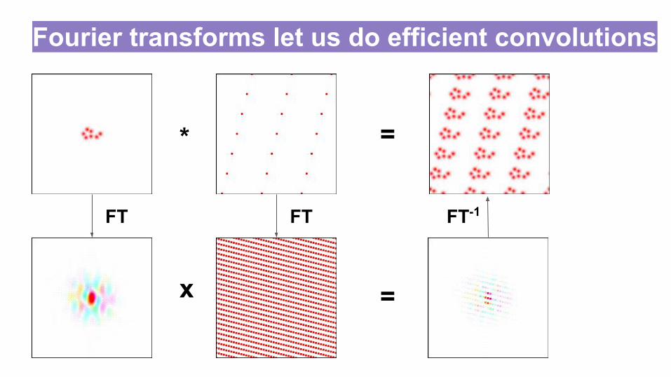
Fourier transforms let us do efficient convolutions

=

=*

x

FT FT FT-1

Scattering and lensing are like Fourier transforms

Y(k) = F(k)CTF(k) + noise(k)

f(x) = projection image of electrons through the specimen

F(k) = FT( f(x) )

y(x) = IFT( Y(k) )

y(x) = image we record on our electron cameras

The linear Fourier imaging model

The 2D Fourier transform lets us separate information at different scales in images


x

FT-1

Fourier transforms let us align noisy images

M: a noisy, off-center particle image

T: a clean, centered template image

The cross-correlation mapwith localization peak

The better the match, the larger the peak

The matched-filter or cross-correlation algorithm:FT-1[ FT(M) x FT(T)* ] = cross-correlation map

We can divide an image into resolution shells and compute cross-correlation for each shell

If we have two images, we can use the Fourier Shell Correlation (FSC) curve to find the resolution where they become inconsistent with each other

FSC curves: - resolution-dependent cross-correlation- resolution-dependent consistency metric for structures- commonly used as measure of resolution

Fourier transforms let us average 2D images in 3DIn electron microscopy, we want to average 2D projection images

together to form a 3D volumetric (‘density’) image… but how?

Forward process: e- beam forms projection image from 3D structure

Inverse problem: Can we recover 3D structure from projection images?

Fourier transforms let us average 2D images in 3D

Images can be averaged in real-space or averaged in reciprocal space and then inverse Fourier transformed

Fourier transforms let us average 2D images in 3DThe projection-slice theorem:

If I take a 2D projection through a 3D object and fourier transform it,I get a 2D slice of the object’s 3D fourier transform.

If we project from a different viewpoint, the slice we get is from that viewpoint


This gives leads to a reconstruction algorithm for solving EM structures:

1. Project an initial 3D density from many views use the projection-slice theorem

2. Match experimental images to projections use the cross-correlation algorithm

3. Calculate a new 3D density from aligned imagesuse the projection-slice theorem

4. Iterate this process until 3D density stops improving

Fourier transforms in digital signal processing

Documents

Transcript of Fourier transforms in digital signal processing