Fourier Transform (FT) NMR and Determination of · PDF fileFourier Transform (FT) NMR and...
32
1 Fourier Transform (FT) NMR and Determination of Molecular Diffusion Coefficients by Pulse Field Gradient (PFG) Experiment for Unknown Samples -Revised and PFG implemented by Yoshitaka Ishii & Dan McElheny 10/19/2012 -Revised by Igor Bolotin 12/19/2011 1. Outline of Basic NMR Principles Nuclear magnetic resonance (NMR), as all spectroscopic methods, relies upon the interaction of the sample being examined with electromagnetic radiation, here in a range of radio frequencies (1- 1000 MHz). To absorb a photon of electromagnetic radiation, the transition energy ΔE sample due to the interaction of a nuclear spin in the sample with a magnetic field must match that of the absorbed radiation at a frequency of as ΔE sample = E photon = ħω = hν = hc/λ (1-1) The NMR experiments will provide a broad range of information on a sample; in particular how the NMR frequency can be used to determine structural and dynamical data. Angular Momentum and Spin Classically, a rotating particle possesses angular momentum. The nucleus of an atom can be visualized as “rotating” and, consequently, has a spin angular momentum I. This angular momentum is intrinsic to the nucleus, rather than the angular momentum arising from the molecule’s spinning in space. While employing an analogy of spin with a rotating particle may be instructive, ultimately it must be treated quantum mechanically. The magnitude of the spin angular momentum is given in quantum mechanics by: ħ [I(I +1)] ½ I = 0, 1/2, 1, 3/2, … (1-2) where ħ is Planck’s constant h divided by 2π and I is the spin angular momentum quantum number or the “spin” of the nucleus. I has a quantized z-component: I z = ħm m = −I, …, 0, …, I (1-3) where m is the magnetic quantum number with 2I +1 values. (The z-component is important as the direction of the static magnetic field is chosen as the z axis and the component of the magnetic moment which will interact with this magnetic field generated by the NMR spectrometer lies along this axis.) Note the parallel between the orbital angular momentum quantum number l and magnetic quantum number m l for the electron in a hydrogen atom and the I and m quantum numbers here.
Transcript of Fourier Transform (FT) NMR and Determination of · PDF fileFourier Transform (FT) NMR and...

1
Fourier Transform (FT) NMR and Determination of Molecular Diffusion Coefficients by Pulse Field Gradient (PFG) Experiment for Unknown Samples
-Revised and PFG implemented by Yoshitaka Ishii & Dan McElheny 10/19/2012 -Revised by Igor Bolotin 12/19/2011
1. Outline of Basic NMR Principles
Nuclear magnetic resonance (NMR), as all spectroscopic methods, relies upon the interaction
of the sample being examined with electromagnetic radiation, here in a range of radio frequencies (1-
1000 MHz). To absorb a photon of electromagnetic radiation, the transition energy ΔEsample due to the
interaction of a nuclear spin in the sample with a magnetic field must match that of the absorbed
radiation at a frequency of as
ΔEsample = Ephoton = ħω = hν = hc/λ (1-1) The NMR experiments will provide a broad range of information on a sample; in particular how the
NMR frequency can be used to determine structural and dynamical data.
Angular Momentum and Spin
Classically, a rotating particle possesses angular momentum. The nucleus of an atom can be
visualized as “rotating” and, consequently, has a spin angular momentum I. This angular momentum
is intrinsic to the nucleus, rather than the angular momentum arising from the molecule’s spinning in
space. While employing an analogy of spin with a rotating particle may be instructive, ultimately it
must be treated quantum mechanically. The magnitude of the spin angular momentum is given in
quantum mechanics by:
ħ [I(I +1)]½ I = 0, 1/2, 1, 3/2, … (1-2)
where ħ is Planck’s constant h divided by 2π and I is the spin angular momentum quantum number or
the “spin” of the nucleus. I has a quantized z-component:
Iz = ħm m = −I, …, 0, …, I (1-3)
where m is the magnetic quantum number with 2I +1 values. (The z-component is important as the
direction of the static magnetic field is chosen as the z axis and the component of the magnetic
moment which will interact with this magnetic field generated by the NMR spectrometer lies along
this axis.) Note the parallel between the orbital angular momentum quantum number l and magnetic
quantum number ml for the electron in a hydrogen atom and the I and m quantum numbers here.

2
Nuclei of all elements are composed of protons (p) and neutrons (n), both of which have spin
I = 1/2. Thus the total nuclear spin is the sum of the spins of all the nucleons. The quantum treatment
indicates that protons and neutrons pair up separately and that even numbers of either have zero spin
angular momentum. The model leads to the three cases summarized in Table I.
Table I. Distinct Ways to Combine Spin of the Nucleons in an Atom
Spin Nucleon Description Examples
I = 0 even numbers of both p and n 12C: 6p, 6n
16O: 8p, 8n
I = n (integer) odd numbers of both p and n 2H: 1p, 1n, I = 1
10B: 5p, 5n, I = 3
I = n/2 (half integer) even p (n) and odd n (p) 13C: 6p, 7n, I = 1/2
23Na: 11p, 12n, I = 3/2
Nuclear Magnetic Moment
Classically, if a rotating particle is charged, it generates a magnetic dipole which creates a
magnetic field. The dipole has a magnetic moment. Associated with nuclear spin angular momentum
is the nuclear magnetic moment μ which can interact with a magnetic field:
μ = γ I (1-4)
where γ is the magnetogyric ratio, a constant characteristic of each nuclide. The magnetic moment
also has a quantized z-component:
μz= γIz = γħm (1-5)
Table II. Properties of Selected Nuclides
Nuclide I γ × 107 rad (Ts)-1 % Natural Abundance
Resonance
Frequency1 [MHz] 1H 1/2 26.7519 99.985 100
2H 1 4.1066 0.015 15.351
13C 1/2 6.7283 1.108 25.144
23Na 3/2 7.0801 100 26.466
1relative to a proton frequency of 100 MHz
Protons and neutrons are not actually true elementary particles but consist of charged fundamental
particles known as quarks. As such, both protons and neutrons contribute to the spin and can also
contribute to the nuclear magnetic moment, μ. However I = 0 spins have no spin and, thus, no

3
magnetic moment. Table II summarizes properties of the four nuclides which will be encountered in
the NMR laboratory experiments.
Nuclear Spin in an External Magnetic Field (Zeeman Effect)
There is no preferred orientation for a magnetic moment in the absence of external fields. In
the absence of B0, the magnetic moments of individual nuclei are randomly oriented and all have
essentially the same energy. Application of an external magnetic field removes the randomness,
forcing the nuclei to align with or against the direction of B0. This change from a random state to an
ordered state is known as polarization. Such polarization means there is a difference in the population
of the various spin states.
Classically, in the presence of an external magnetic field B0 the energy of a magnetic moment
μ depends on its orientation relative to the field:
E = − μ . B0 (1-6)
which is a minimum when the magnetic moment is aligned parallel to the magnetic field and a
maximum when it is anti-parallel. From the quantum mechanical prospective, when a nucleus is
introduced into a magnetic field its magnetic moment will align itself in 2I +1 orientations (number
of values of the m quantum number) about the z direction of B0 where the energy is given by:
Em = − μz B0 = − γħmB0 (1-7)
For an I = 1/2 nucleus, there are only two orientations for the magnetic moment μ: 1) a lower energy
orientation parallel to B0 with a magnetic quantum number m = 1/2 often referred to as the α spin
state and 2) a higher energy anti-parallel orientation with m = −1/2 referred to as the β spin state. For
an I = 1 nucleus there are three possible orientations for the magnetic moment, these states are
illustrated below.
Directional quantization of the angular momentum P in
the magnetic field for nuclei with I=½ and 1
Energy level schemes for a nucleus
spin quantum number ½

4
Transition Frequencies
NMR spectroscopy induces transitions between adjacent nuclear spin energy states (the
selection rule is Δm = ±1). The energy change for a nucleus undergoing an NMR transition from the
spin state characterized by the magnetic quantum number m to the state with quantum number m − 1
is:
ΔE = Em−1 – Em = [−γħ(m −1)B0] – [−γħmB0] = γħB0 (1-8)
Equation (8) follows from the previous discussions. The difference between the z-component of the
angular momentum of adjacent m states is ħ [Eq. (2)]. This difference is multiplied by γ to obtain the
difference in the magnetic moment z-component [Eq. (5)]. This result is then multiplied by the
magnetic field strength to obtain the energy difference between adjacent m states in a magnetic field
[(Eq.7)].
The frequency ν of the electromagnetic radiation used to induce an NMR transition between
adjacent m levels in an external magnetic field B0 is found from Eq. (1)
ν = ΔE/h = γħB0/h = γB0/2π (1-9)
The units of frequency (ν) are cycles/second, hertz (Hz) in SI units. In NMR spectroscopy, it is often
more convenient to use angular frequency (ω) with units of radians/second. Since one cycle equals
2π radians:
ω ≡ 2πν (1-10)
Since cycles and radians are not SI units, both ν and ω have the same SI units (s-1). The angular
frequency of an NMR transition is more commonly written as:
ω0 = γB0 (1-11)
which is the Larmor equation. Note that the use of ω
eliminates the occurrence of 2π in the Larmor equation. The
Larmor frequency has two important physical
interpretations. It is the frequency of the electromagnetic
radiation that induces a transition between nuclear spin
quantum states in the magnetic field. It is also the
precessional (or rotation) frequency of the nuclear magnetic
moment about the magnetic field as represented here for a
spin-1/2 nucleus (i. e. a spin with I = ½).
Precession of nuclear dipoles

5
TkE
low
highe
N
N
Boltzmann Statistics
In the presence of an external magnetic field, different nuclear spin states (with different
values of m) have different energies. The energy difference is proportional to B0. At thermal
equilibrium, these states will also have different populations, their ratio given by the Boltzmann
equation:
(1-12)
with Nhigh and Nlow the respective populations of the
upper and lower spin states, ΔE =Ehigh − Elow the energy
difference between the two states, k the Boltzmann
constant, and T the absolute temperature. In currently
achievable magnetic fields, the difference between
nuclear spin energy levels ΔE is much smaller than kT,
implying that Nlow is only very slightly in excess of
Nhigh. For 1H in a 9.4 Tesla field (400 MHz) and 300 K one obtains a population ratio N(α)/N(β) of
1.000064, i.e., for one million spins in the upper β state there are one million and sixty-four in the
lower energy α state! It is the excess 64 spins that respond to the NMR experiment and create the net
magnetization M0. To summarize, the larger B0 is the greater the energy difference ΔE between the
levels and the larger the ΔE the more excess population exists in the lower energy state (waiting to be
excited to the higher level).
The Pulse NMR Experiment and Fourier Transform NMR
The excess of nuclear spins in the lower energy α spin state is illustrated below on the far left.
In the presence of the B0 magnetic
field the precessing spins are distributed
equally about the z-axis. Their precessional
frequency ω0 is given by the Lamor equation
[Eq. (11)]. The vector sum of the individual
μ vectors [Eq. (4)] yields a net equilibrium
magnetization Mo along the positive z-axis.
(Due to the precession about the z-axis, the
Distribution of the precessing nuclear dipoles (total number N (=N+N) around the double cone. As N>N there is a resultant macroscopic magnetization M0

6
x and y components of the individual μ vectors sum to zero, leaving only the z component μz [(Eq.
(5)]). Excitation of the nuclei from the lower energy α spin state to the higher energy β spin state is
achieved with an oscillating radio frequency magnetic field B1 applied with a transmitter coil as a
short duration pulse along the x-axis (RF pulse). The oscillating magnetic field can be viewed as a
rotating magnetic field. When the rotating frequency of B1 is equal to the precession frequency of the
nuclear moments (ω0), B1 excites nuclei in the α spin state to the β spin state. This causes the net
magnetization M0 to rotate about the x-axis tipping it from the z-axis into the yz-plane. (One can
completely transform the z magnetization into y magnetization if the duration of the pulse is the
length of a π pulse, a 90° pulse.) The component of the magnetization in the xy plane, initially along
the y-axis (My) precesses about the z-axis at the precession frequency ω0. The net magnetization
along the y-axis is detected with an antenna coil illustrated with an eye in the figure on the previous
page.
We will be conducting the experiments in a pulsed Fourier Transform NMR spectrometer
equipped with a superconducting magnet; a diagram of the spectrometer is shown below along with a
schematic of its operation. In the
pulse method of acquiring an NMR
spectra, all the nuclei of one species
in the sample are quickly excited
simultaneously by a “hard” pulse of
energy for a very short (~s)
duration of time. The power of this pulse is on the order of several
Watts at a range of frequencies such that all the nuclei absorb the
energy. This pulse of energy is applied perpendicular to the z-direction
of the applied magnetic field. As a result, the net magnetization of the
sample (M0) is itself turned 90°, and is thus “tipped” into the xy plane
as shown here.
This type of pulse is often called a pulse (as = 90°). Now that the magnetization
vector has turned on its side into the xy plane, the magnetization begins to precess which is detected
by a coil of wire. The wire experiences an oscillating magnetic field, and like a power plant, begins
to generate current which is amplified and detected by the electronics of the NMR spectrometer. The
signal will oscillate and eventually decays as the nuclear spins begin to precess incoherently from

7
eachother and relax to their ground state. The signal is called a FREE
INDUCTION DECAY (FID). Here is a typical example
With respect to the eye, y-axis magnetization rises and falls in a
sinusoidal manner as the vector precesses about the z-axis. The amplitude
of the signal decays with time as nuclei in the higher energy β spin state return back to the lower
energy α state in a process known as nuclear spin relaxation. If the molecule has only a single
chemical shift, the signal appears as a simple decaying sine wave and the chemical shift in hertz is
the frequency of the sine wave relative to a reference frequency. Most molecules have many nuclei
with many different chemical shifts and correspondingly many different precession frequencies. The
B1 field actually contains a broad band width of frequencies that excite all the nuclei in a molecule at
the same time, and the net magnetization along the y-axis is the sum of the magnetization of each set
of equivalent nuclei, all precessing at different frequencies. The resulting complex waveform is
called the free induction decay (FID) or the time domain spectrum. It is a measure of y-axis
magnetization My as a function of time after the B1 pulse.
This signal is not very useful in its present form; to change it into an actual NMR spectrum,
we have to take the Fourier Transform
of the signal which is accomplished by
the following mathematical
relationship:
Spectrum () =
tetsignal ti )(
(13)
What the Fourier Transform shows
is how much of what oscillating frequencies
can be added together to equal the original
signal. Here are some examples of FIDs and
their Fourier Transforms (F.T.) where you
can see how the two are related:
Note that the frequency of the oscillations
changes the position of the peak. If the oscillating signal decays more quickly, the peak becomes broader due to the
fact that the FFT has less “signal”. This causes the FFT procedure to be less “sure” of the true frequency which is
why the peak broadens. Further, if there are clearly two frequencies overlapping, which appear as “beats” in the
FID, the FFT will reveal which two (or more!) frequencies are present.

8
Nuclear Spin Relaxation
How do the nuclei rid themselves of the energy that they have absorbed from the NMR
spectrometer? The precession of spins in the xy-plane does not last forever. It decays due to three
distinct effects:
1. Spin-Lattice (or Longitudinal) Relaxation, T1 (mechanism which involves a net transfer of
energy from spin system to surroundings to reestablish Boltzmann distribution). Application of an
RF pulse and the consequent rotation of the net magnetization Mo from the z-axis is a disruption of
the thermal equilibrium of the spins. After being disturbed by an RF pulse thermal relaxation occurs
to reestablish equilibrium. This process involves a net transfer of energy from the spin system to the
environment until the populations of the energy states reach equilibrium, the Boltzmann distribution
given in Eq. (12). It is attributable to electromagnetic interactions between the nuclei and the
surrounding particles causing transitions between the alpha and beta spin states (when I = ½). As it is
the coherent combination of these spin states that contribute to the magnetization rotating in the xy-
plane, the result is a gradual decay of these coherent combinations and a return to the state of thermal
equilibrium in which the magnetization is in the z-direction and therefore no longer capable of
inducing a signal in the antenna coil. How fast the spins regain equilibrium is a measure of the
coupling of the spins to their environment. The approach to equilibrium is exponential and
characterized by a time constant denoted by T1, called the spin-lattice or longitudinal relaxation time.
- refers to the return to equilibrium of the z-component of the net magnetization of the sample at a
rate of 1/T1 (a rate is generally expressed in units of inverse time, i.e. s-1)
- the rate of change of Mz is described by the first order kinetic relationship:
1
0
T
MM
dt
dM zz (1-14)
The solution is: 00
/ )0()( 1 MMtMetM zTt
z (1-15)
2. Spin-Spin (or Transverse) Relaxation, T2 (mechanism which causes spin vectors to become
evenly distributed in xy-plane without transfer of energy to the surroundings). With the passage of
time after an RF pulse tips the net magnetization Mo from the z-axis, the magnetic moments interact
with one another by magnetic dipole interactions. Nuclei in any given substance are generally located
in several different molecular environments, each with a slightly different Bo. In each of these
regions the precession frequency will be perturbed to a slightly different extent. The result is a
collection of regions rotating at slightly different frequencies producing a gradual loss of phase

9
coherence (precessing as a group) and a decay of the resultant magnetization. This loss of transverse
magnetization is characterized by a time constant denoted by T2, called the spin-spin or transverse
relaxation time.
- With the total energy of the system remaining the same, the entropy-driven exhance of spins
between neighboring nuclei results in a loss of the xy component of the magnetization. The rate of
changes of Mx and My are described by the first order kinetic relationships:
2T
M
dt
dM xx and 2T
M
dt
dM yy (1-16)
The solutions are:
2/)( Ttx etM and 2/)( Tt
y etM (1-17)
3. The magnetic field is not perfectly uniform. Nuclei in different parts of the sample precess at
slightly different frequencies and get out of phase with one another, thereby gradually decreasing the
net magnetization of the sample.
Spin-Lattice Relaxation Mechanisms
In many cases, the same physical relaxation mechanisms determine T1 and T2 so that they are
then equal. In spectroscopies involving higher energy excitation such as in the ultraviolet or visible
region of the electromagnetic spectrum, the return to the ground state of an excited molecule is very
rapid. The situation is quite different in NMR where the small energy difference between nuclear
spin states means that spontaneous emission is very slow. (The lifetime of an unperturbed excited
nucleus is in the range of years!) Consequently the excited nucleus must be induced to flip its spin
and return to the ground state by some external means. From an analysis of the interaction of
electromagnetic radiation with matter one can conclude that a spin subjected to a fluctuating
magnetic field will be induced to undergo transitions between all available energy levels at a rate that
is proportional to the intensity of the field. The principal mechanisms for producing fluctuating
magnetic fields include:
chemical shift (or shielding) anisotropy
– local magnetic field acting on a nucleus changes the shielding at the nucleus due to tumbling.
dipole-dipole interactions with other nuclei
– interactions similar to that observed between two small bar magnets modulated by molecular
tumbling or by translational diffusion; this is most important for I = ½ nuclei.
interactions with unpaired electrons

10
– This is similar to the dipolar mechanism except that one of the magnetic moments belongs to an
unpaired electron
spin-rotation interactions
– interruption of the coupling between angular momentum due to molecular rotation and nuclear
spin arising from molecular collisions
scalar interactions
– indirect coupling of nuclear spins through electrons; like dipolar mechanisms except that one of
the magnetic moments is that of an electron (and thus requires a quadrupolar nucleus)
quadrupolar interactions
– For nuclei with I > ½ where a nuclear electric quadropole moment exists that interacts with
electric fields
Attributes of 1H NMR Spectroscopy: NMR Chemical Shift
Chemical shift, ppm = 610
Hzin frequency er spectromet
reference offrequency -signal offrequency (1-18)
• The chemical shift is the position on the δ scale (in ppm) where the peak occurs.
• There are two major factors that influence chemical shifts:
1. deshielding due to reduced electron density (due electronegative atoms)
2. anisotropy due to magnetic fields generated by π bonds
Table III – Proton Chemical Shifts

11
Shielding in NMR
Nuclei are shielded by valence electrons surrounding them which circulate in an applied
magnetic field producing a local diamagnetic current in the opposite direction. This diamagnetic
shielding will affect the frequency of radiation necessary to cause a nucleus to spin flip (the
resonance frequency). Therefore nuclei will absorb radiation of slightly different frequencies
depending upon their local magnetic environment, which is determined by the structure of the
compound. Since the magnetic field strength dictates the energy separation of the spin states, and
hence the radio frequency of the resonance, the structural factors mean that different types of nuclei
will occur at different chemical shifts. This is what makes NMR so useful for structure
determination, otherwise all nuclei would have the same chemical shift. Some important factors
include:
• inductive effects by electronegative groups
• magnetic anisotropy
Electronegativity
Electrons around the nucleus create a magnetic field that opposes the applied field. This
reduces the field experienced at the nucleus. Since the induced field opposes the applied field the
electrons are said to be diamagnetic and the effect on the nucleus is referred to as diamagnetic
shielding. Since the field experienced by the nucleus defines the energy difference between the
different spin states, the frequency (and hence the chemical shift δ) will change depending on the
electron density around the nucleus. Electronegative groups decrease the electron density around the
nucleus, and there is less shielding (i.e. deshielding) so the chemical shift increases.
Magnetic Anisotropy
Magnetic anisotropy means
that there is a non-uniform magnetic
field. Electrons in π systems (e.g.
aromatics, alkenes, alkynes, carbonyls,
etc.) interact with the applied field
which induces a magnetic field that
causes the anisotropy. As a result, the
nearby nuclei will experience three
fields: the applied field, the shielding

12
field of the valence electrons, and the field due to the π system. Depending on the position of the
nucleus in this third field, it can be either shielded (smaller δ) or deshielded (larger δ), which implies
that the energy required for, and the frequency of the absorption will change. Here are some
examples:
low field high field down field up field deshielded shielded high frequency low frequency large δ (ppm) small δ (ppm)
COUPLING IN 1H NMR
Spectra generally have peaks that appear in clusters due to coupling (scalar, spinspin, J-
coupling) with neighboring protons The coupling constant J (usually in frequency units, Hz) is a
measure of the interaction between a pair of protons.
Before looking at the coupling, examine the peak assignments
• δ = 5.9 ppm, integration = 1H; deshielded: agrees with the −CHCl2 unit
• δ = 2.1 ppm, integration = 3H; agrees with −CH3 unit.
What about the coupling patterns? Coupling arises because the magnetic field of adjacent protons
influences the field that the proton experiences. To understand the implications of this first consider
the effect the −CH group has on the adjacent −CH3.

13
The methine –CH can adopt two alignments with respect to the applied field. As a result, the
signal for the adjacent methyl −CH3 is split into a doublet, two lines of equal intensity. Now consider
the effect the −CH3 group has on the adjacent −CH. The methyl -CH3 protons have 8 possible
combinations with respect to the applied field, only four of which are magnetically distinct. The
resulting signal for the adjacent methane −CH is split into a quartet, 4 lines of intensity ratio 1:3:3:1.
n + 1 Rule
As protons on a carbon atom experience the magnetic field of protons on adjacent carbon
atoms the signal for a particular proton will be split by these protons into n + 1 peaks where n is
the number of adjacent protons.
Pascal’s Triangle
The relative intensitites of the lines in a coupling pattern is given by a binomial
expansion or more conveniently by Pascal's triangle. Individual resonances are split due to
coupling with n adjacent protons. The number of lines in a coupling pattern is given, in general,
by 2nI + 1 for coupling with n spin I nuclei.
Doublet on CH3 Quartet on CHCl

14
INTERPRETING 1H NMR SPECTRA
What can be obtained from a 1H NMR spectrum:
• number of equivalent types of H - number of groups of signals in the NMR spectrum.
• types of H – chemical shift of each functional group’s protons found in chemically identical
environments are chemically (and usually also magnetically) equivalent; these chemically equivalent
protons will have the same chemical shift.
• number of H of each type - NMR spectrometer can integrate (or calculate the area under each peak) all
peaks to determine the relative numbers of protons responsible for all peaks.
• connectivity - spin-spin splitting (J coupling with the n + 1 rule) – the coupling pattern identifies the
adjacent functional group(s).
Chemical shift
• The chemical shift is the position on the δ scale (in ppm) where the peak occurs.
• There are two major factors that influence chemical shifts: 1) deshielding due to reduced electron
density (due electronegative atoms) and 2) anisotropy (due to magnetic fields generated by π bonds).
Integration
• The area of a peak is proportional to the number of H that the peak represents
• The integral measures the area of the peak
• The integral gives the relative ratio of the number of H for each peak
Coupling
• The proximity of other n H atoms on neighboring carbon atoms, causes the signals to be split into n +1
lines (to first order).
• This is also known as the multiplicity or splitting of each signal.
Table IV. Magnitude of Some
Typical Coupling Constants1
1Magnitude of the coupling
constant is independent of the
strength of the applied field.

15
Attributes of 13C NMR SPECTROSCOPY
It is useful to compare and contrast 1H NMR and 13C NMR as there are certain similarities as
well as differences.
• 12C isotope does not exhibit NMR behavior (nuclear spin I = 0)
• 13C isotope has a natural abundance of 1.108% (of all C atoms)
• Magnetogyric ratio γ for 13C is approximately four times smaller than γ for 1H
• As a result, a 13C nucleus is about 400 times less sensitive than a 1H nucleus in NMR spectroscopy
• 13C-13C coupling is seldom observed due to the low natural abundance of 13C
• Chemical shifts measured with respect to tetramethylsilane, (CH3)4Si (i.e., TMS)
• Chemical shift range is normally 0 to 220 ppm
• Similar factors affect the chemical shifts in 13C as in 1H NMR
• 13C spectra are normally broadband proton decoupled, removing J coupling between 13C and 1H, so peaks
appear as single lines
• Number of peaks indicates the number of distinct types of C
• Long relaxation times (excited state to ground state) mean no meaningful peak area integrations
The general implications of these points are that 13C take longer to acquire, though they tend
to look simpler. Overlap of peaks is much less common than for 1H NMR which makes it easier to
determine how many distinct types of C are present.
Table V. 13C Chemical Shifts. Note the importance of hybridization in the shielding of 13C chemical shifts and
the magnitude of the J coupling with bonded protons, both in the order: sp2 < sp < sp3

16
There are four alcohols with the molecular formula C4H10O
Which one produced the 13C NMR spectrum below?
Interpreting 13C NMR Spectra
The following information can be obtained from a typical broadband decoupled 13C
NMR spectrum (all coupling with 1H removed):
• number of types of C - indicated by number of signals (peaks) in the spectrum.
• types of C - indicated by the chemical shift of each signal.
2. Advanced NMR Experiments to Aid Spectral Interpretation for This Lab
Each dimension of an NMR experiment represents a different observable nucleus. Normal 1H
and 13C NMR look at a single type of nucleus at one time by plotting intensity versus frequency. It is
possible to examine multiple nuclei simultaneously by using the Fourier Transform (FT) technique
coupled with a computer capable of directing RF pulses on both nuclei during the same time period.
In such experiments, intensity is plotted as a function of two frequencies generally in the form of a
contour plot. This part of the NMR lab will examine a useful one-dimensional technique DEPT and
two different two-dimensional NMR experiments: HETCOR and COSY.
Molecular Diffusion Measurements by Pulse Field Gradient (PFG) experiments: In this
experiment, two magnetic field-gradient pulses are applied at the beginning and the end of the
molecular diffusion period for a series of different field gradient strengths (G). Due to the
molecular diffusion process during the period , the 1H NMR signals decay exponentially with
respect to G2 as s() = exp(-aDG2). The rate of the exponential decay for each 1H species is
proportional to the molecular diffusion coefficient D, which characterizes how quickly molecule
travels in a solution. Thus, this PFG experiment provides information on the molecular identity for
different 1H peaks for a mixture sample.

17
DEPT (Distortionless Enhancement by Polarization Transfer): A 1D experiment used for
enhancing the sensitivity of the carbon signal and for editing of 13C spectra. The sensitivity gain
comes from starting the experiment with proton excitation and subsequently transferring the
magnetization onto carbon (via the process known as polarization transfer). This gain arises due to
the larger population differences associated with protons, which are four times bigger than those of
carbon (γ is four times larger). DEPT alters the amplitude and sign of the carbon resonances
according to the number of directly attached protons, allowing the identification of carbon
multiplicities.
45 decoupler pulse - carbon spectrum contains only carbons with protons attached (quaternary
carbons are not observed).
90 decoupler pulse - carbon spectrum contains only carbons with a single attached proton,
methine CH
135 decoupler pulse - carbon spectrum with methyl (CH3) and methine (CH) carbon peaks up,
methylene (CH2) carbon peaks down (negative)
HETCOR: A 2D experiment used to identify couplings between heteronuclear spins. Most
often employed to correlate carbons with their directly bonded protons by the presence of cross-
peaks in the 2D spectrum. HETCOR relies on scalar coupling (spin-spin or J coupling) between the
different nuclei. The HETCOR spectra in our experiments plot proton versus carbon with 1D spectra
displayed along the appropriate axis. The 2D peaks show which protons are coupled to which
carbons.
COSY: A 2D experiment used to identify nuclei that share a scalar (J) coupling. The
presence of off-diagonal peaks (cross-peaks) in the spectrum directly correlates the coupled partners.
Most often used to analyze coupling relationships between protons, but may be used to correlate any
high-abundance homonuclear spins. The COSY spectra in our experiments plot the proton spectrum
versus itself. The 2D peaks show which 1H are coupled over three bonds.
For the 7 experiments on your unknown, include:
1. 1H spectrum with integration and tabulated peak assignments with reasoning
2. 13C spectrum and tabulated peak assignments with reasoning
3. DEPT 45. 90. 135 with explanations
4. HETCOR – explain C-H correlations
5. COSY – explain H-H correlations

18
As you are obtaining these spectra to aid in the identification of your unknown structure
you should explain how the 1H and 13C spectra along with the DEPT, HETCOR, and COSY data
allowed you to determine the structure. Be sure to draw the structure!
For the PFG Diffusion experiment (be sure to do the appropriate regression analysis). You
present the following data after the data analysis.
1. Stacked plots of the 1H NMR spectra for different fractional PFG strength (fn)
2. Table of peak intensities measured from the stacked plots versus fn for each peak
3. Plots of peak intensity measured from the stacked plots versus fn for each peak
4. Table of a normalized signal In = Sn/S1 vs fn2
5. Plot of In vs fn2 with a fitting curve
6. Determine the diffusion coefficients D for all of the peaks.
3. Guide on Pulse Field Gradient for Diffusion Measurements
Magnetic Field Gradient, NMR Spectroscopy, and Magnetic Resonance Imaging (MRI)
NMR experiment also allows one to examine molecular diffusion process in solution. For this purpose, a pulse field gradient is typically used. A field gradient is the linearly tapered magnetic field, which allows us to identify the location of a molecule. When a field gradient is applied, a static magnetic field B0(x, y, z) is dependent on the location of the molecule as
B0(x, y, z) = B0 + GX (x – x0) + Gy(y – y0) + GZ (z – z0), (3-1)
where Gx, GY, GZ denote the field gradient along the x, y, z axes, respectively. Now assume a field gradient pulse is applied along the Z axis, then we obtain
B0(x, y, z) = B0 + GZ (z – z0). (3-2)
The NMR frequency NMR under the magnetic field now depends on the position of the molecule z as
NMR(z) = - B0(x, y, z) = - B0 - GZ (z – z0) = 0 - GZ (z – z0), (3-3)
where 0 is the NMR frequency when there is no field gradient (Larmor frequency). For simplicity, assume that Z = -(z – z0) and G = Gz. Then, eq. (3-3) is rewritten as
NMR(Z) = 0 + G Z, (3-4)

19
Namely, the location of the molecule Z can be detected by monitoring the shift in the NMR frequency under a field gradient. This position dependent NMR frequency is a basis of MRI imaging used in hospitals.
Figure 3-1. NMR frequency depends on the Z position of the molecule under a magnetic field gradient.
Figure 3-2. Pulse sequence for diffusion measurements using field gradient spin echo.
Principle of diffusion experiments by a pulse field gradient
Now, assume that we perform a spin echo experiment listed in Fig. 3-2 under two field gradient pulses (rectangles accompanied by G). The field gradient pulse provides a position
dependent shift of the NMR frequency given by GZ. During the first field gradient pulse having a
pulse width of , a spin magnetic moment is subject to a rotation by GZ x .
A spin echo sequence changes the direction of NMR nutation caused by the field gradient. Now, assume that your molecule is positioned at Z1 and Z2 at the first and second field gradient
pulses, respectively. If a molecule does not move during the period (i.e. Z1 = Z2), the net rotation
observed during the echo period is given by [NMR(Z2) - NMR(Z1)] =[NMR(Z2) - NMR(Z2)] = 0, where δ denotes a pulse width of the field gradient. However, if molecular diffusion takes place
Z

20
during and if the locations before and after the pulse are different (i.e. Z2 Z1), the net rotation due to the nutation is given by
{NMR(Z1) - NMR(Z2)} = G(Z2 – Z1) , (3-5)
where we assumed that the gradient pulse is strong and the diffusion during δ is negligible. Thus, the
signal detected during the detection period is attenuated by a factor s(GZ, )
s(GZ, , ) = cos[{NMR(Z1) - NMR(Z2)}] = cos{G (Z2 – Z1)}. (3-6)
The probability that a molecule diffuses by a distance r = Z2 – Z1 along the z-axis during the period is defined by Einstein Stokes diffusion process and given by
P(r) = P0 exp(-r2/4D), (3-7)
where D is a diffusion constant of molecule and P0 = (1/4Dπ)1/2. Then, the average attenuation of the signal from eq. (6) is given by
<s(G, , )> = < cos[{0(Z1) - 0(Z2)}] >
= < cos{G (r)}P(r) > = a/4)exp(-q})G ( cos{) /4Dr exp(- P 20
20 Padrr
, (3-8)
Where q = (γGδ), a = 4D, and (a)1/2P0 = 1. In summary, the diffusion attenuation factor I(G, , ) is given by
I(G, , ) = <s(G, , )> = exp(- q2D). (3-9)
When the diffusion during is not negligible, we use a modified equation
I(G, , ) = exp[- q2D(-/3)]. (3-10)
The diffusion constant is related to the hydrophobic radius of the molecule Rmol by
D = kBT/6Rmol, (3-11)
where kB is the Boltzmann constant, T Is the temperature, is viscosity of the solvent. Assuming the molecules A and B have spherical shapes and the density of these molecules are the same, the ratio of the molar masses are estimated from the diffusion constants as
DA/DB = RB/RA ~ (MB/MA)1/3, (3-12)
where DA and DB should be measured in the same solvent and at a common temperature. Estimate the molar mass of your unknown from D with DH2O and MH2O.

21
Data Analysis Protocol
A group receives a stacked plot of the spectra that were collected for a series of different gradients Gn (n =1, 2, .. N) for the unknown sample in a solvent (water), for which diffusion constant D is known (see Fig. 3). For a peak for the control sample (i.e. water), signal intensities for a varied gradient Gn are given as
Scon(n) = S0 con exp[-(γGn δ)2Dcon(-/3)], (3-13)
where Gn denotes a field gradient for the n-th data points and S0 con is a constant that represents the signal intensity when Gn = 0. Now, we define the strength of the field gradient Gn using a fractional strength fn as Gn = Gmaxfn, where Gmax is the maximum gradient of the instrument. For example fn is denoted as 10% or 0.1 with respect to Gmax (Typically, we change fn from 5% to 95%). Then eq. (13) is rewritten as
Scon (n) = S0 con exp[-(γGmax δ)2Dcon(-/3) fn2], (3-14)
Now we define p as p = (γ Gmaxδ)2(-/3). Here p is a constant that does not depend on the sample or the analyte molecule. Then, the equation is simplified as
Scon(n) = S0 con exp[-Kcon fn2], (3-15)
where Kcon =p x Dcon. Using the peak table, plot Scon(n) along the Y-axis with respect to fn2 along
the X-axis for each peak, and you find
Y = exp[-Kcon X], (3-16)
By using a curve fitting of the plot to the exponential curve using software (such as Excel), you find Kcon = p x Dcon as a rate of the exponential decay. Once you get Kcon, p can be easily found from the known Dcon (if H2O is used as a control, DH2O = 2.299 x 10⁻⁹ m2s-1 at 25 ̊C) by
p = Kcon/Dcon. (3-17)
For a signal A ( or B, C, …) of your unknown, similarly,
SA(n) = SA 0 exp[-KA X], (3-18)
where kA =p x DA. Again, find KA by plotting SA(n) with respect to X = fn2. Then, once you find
kA, obtain DA from
DA = Dcon x (KA/Kcon) (3-19)
Estimate the molar mass of the unknown from eq. [9] (DA/DB = RB/RA = (MB/MA)1/3) as
MA ~ Mcon x (Dcon/DA)3. (3-20)
Hint: If the peaks A and C come from the same molecule for example, determined DA and DC should be similar within the range of the error.

22
Figure 3-3. Example data for pulse field gradient molecular diffusion experiment.
4. Guide on Other Advanced Experiments
DEPT: Distortionless Enhancement by Polarization Transfer
A 1D experiment that utilizes polarization transfer from a
nucleus with a relatively larger magnetogyric ratio γ to one with a
smaller γ to increase the signal from the latter nucleus, here from 1H to 13C. By changing the last proton pulse from 45° to 90° to
135° the multiplicity of the carbon nucleus
can be determined.
Observed 13C signals are modulated
by the 13C−1H coupling constant so that
when 1) θ = 45°, signals from all CH, CH2,
and CH3 carbons are observed (no
quaternary C or C attached to D, as in a
deuterated solvent), 2) θ = 90° signals seen from only CH
carbons, and 3) θ = 135° signals from all CH, CH2, and CH3
carbons but the CH2 signals are negative.
On the right are the proton decoupled 13C spectrum and
DEPT spectra at 45°, 90°, and 180° for the compound on the

23
left. DEPT 45 only shows C with a directly bonded H, DEPT 90 CH, and DEPT 135 has
negative peaks for CH2 C atoms.
DEPT 90 and 135 spectra on the left are sufficient to identify which of
A-E is the structure of the compound. The uppermost spectrum is the 1H decoupled 13C spectrum.
HETCOR: HETeronuclear CORrelation (also called 13C−1H COSY)
A 2D heteronuclear
correlation experiment where cross
peaks yield information about the
connectivity of two different spin
coupled spin 1/2 nuclei, here
protons with 13C nuclei. The
experiment takes advantage of the
large one-bond heteronucler J
coupling for polarization transfer
between the 1H and 13C nuclei. The
experiment can be modified to give
coupling information over more
than one bond.
The HETCOR experiment involves 13C-1H correlation by polarization transfer. It encodes
the proton chemical shift information into the observed 13C signals and yields cross signals for
all 1H and 13C nuclei that are connected by 13C-1H coupling over one bond.

24
1D 1H NMR plotted vs. 1D 13C NMR; cross peaks observed
at intersection of the x and y values denoting the CH
interactions. Peak A shows that the H at ~ 4 is bonded to the
C at ~ 60 ppm. Peak B shows that H at ~ 1.8 ppm is bonded
to C at ~18 ppm. The quaternary C is identifiable as no cross
peak appears (*). HETCOR pulse sequence
COSY: COrrelation SpectroscopY
A 2D homonuclear correlation experiment where cross peaks yield information on the
protons which are spin-spin coupled to each other. The experiment uses polarization transfer
between the coupled spins. The technique can be modified to yield COSY spectra for four-, five-,
and occasionally six-bond couplings.
P
COSY pulse sequence
COSY experiment involves 1H-1H correlation by polarization
transfer. It encodes the proton
coupling information into the
observed 1H signals and yields
cross signals for all 1H that are
coupled over three bonds.
1D 1H NMR plotted vs. 1D 1H NMR generating a 2D xy plot. If a signal on the x-axis has an
interaction with a signal on the y, a cross peak is observed at the intersection of the x and y
values, denoting the interaction. The peaks on the diagonal represent the 1H spectrum and the
COSY is symmetric with respect to the diagonal. Peak A indicates that the peak at ~ 6.9 ppm is

25
proton coupled to the peak at ~ 1.8. Peak B indicates that the peak at ~ 4.2 ppm is coupled to the 1H at ~1.3.
5. Laboratory Report Requirements
The following information is required in your laboratory report for this experiment.
Please note that both students of each group are required to have all copies of all spectra,
printouts, and any other data, notes, etc., recorded during the laboratory meetings.
5. Laboratory Report Requirements
The following information is required in your laboratory report for this experiment. Please
note that both students of each group are required to have all copies of all spectra, printouts, and any
other data, notes, etc., recorded during the laboratory meetings.
I. Abstract (1 page)
II. Introduction (3-4 pages)
• Introduce what is NMR (How is NMR used in chemistry and other fields?
• Briefly summarize the principles of NMR spectroscopy (What is detected in NMR? How is the
NMR signal observed? What are 13C NMR and 1H NMR?)
• Briefly discuss how DEPT and 2D 1H/13C correlation NMR can be used.
• Briefly discuss the pulse field gradient experiments for characterizing molecular diffusion.
III. Spectra
• 13C spectrum of your unknown, with 13C chemical shift assignments made and your prediction of
the sample name and chemical structure of the compound (carbons should be labeled for assignments
as CA, CB, CC, …). Indicate the numbers in the spectrum for assignments.
• 1H spectrum of your unknown, with 1H chemical shift assignments and chemical structure of the
compound (protons should be numbered for assignments as HA, HB, HC). Indicate the numbers in
the spectrum for assignments.
• 13C DEPT 45, 90, 135 spectra of the unknown with assignments made.
• A contour plot of 2D spectrum (COSY, HETCOR) of your unknown sample and assignments of
13C and 1H.
• A stack plot of 1H NMR spectra for varied pulse field gradient strengths.

26
IV. Data sheet and calculations
For the PFG Diffusion experiment
(1) Table of peak intensities measured from the stacked plots versus fn for each peak
(2) Plots of peak intensity measured from the stacked plots versus fn for each peak
(3-1) Table of a normalized signal In = Sn/S1 vs fn
(4-2) Table of a normalized signal In vs fn2
(5) Plot of Y = In vs X = fn2
(6) Use Excel or other program to obtain the best fit curve for Y = Aexp(-BX) for (6). If f12~ 0, you
can assume that A = 1. If the curve does not fit to the exponential curve well, check the calculation
in (5-1) and (5-2) again.
(7) Determine the diffusion coefficients D for all of the 1H peaks using the B value. Show sample
calculations.
V. Results
Peak table and summary of assignments and the calculated diffusion coefficients D.
(1) Peak table for your 13C spectrum. List ppm positions and your assignments
Indicate the chemical structure and numbering clearly.
Example.
Signal assignments for 13C NMR spectrum Peak position
(ppm)
182 125 55 40 32 25
Peak # a b c d e F Assignments CA CP CB CC CD CQ
Molecules Mol A Mol B Mol A Mol A Mol A Mol B
CPH3-CQHCl2
Mol A (Name) Mol B (Name)
27
(2) Peak table for your 1H spectrum. List ppm positions and your assignments with D values
(obtain from the analysis in Sec .3). Indicate the chemical structure and numbering clearly.
Signal assignments for 1H NMR Peak position
(ppm)
1.3 2.1 3.5 4.6 6.2 7.5
Peak # a b c H2O d E Assignments HB HC HD H2O HP HQ D (10-9 m2/s) 3.2 1.3 2.3 0.5 5.2 6.3
Molecule Mol A Mol A Mol A H2O Mol B Mol B As for the structure follow the above example & Label 1H clearly.
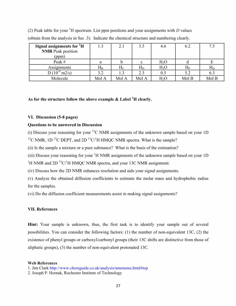
VI. Discussion (5-8 pages)
Questions to be answered in Discussion
(i) Discuss your reasoning for your 13C NMR assignments of the unknown sample based on your 1D 13C NMR, 1D 13C DEPT, and 2D 13C/1H HMQC NMR spectra. What is the sample?
(ii) Is the sample a mixture or a pure substance? What is the basis of the estimation?
(iii) Discuss your reasoning for your 1H NMR assignments of the unknown sample based on your 1D 1H NMR and 2D 13C/1H HMQC NMR spectra, and your 13C NMR assignment.
(iv) Discuss how the 2D NMR enhances resolution and aids your signal assignments.
(v) Analyze the obtained diffusion coefficients to estimate the molar mass and hydrophobic radius
for the samples.
(vi) Do the diffusion coefficient measurements assist in making signal assignments?
VII. References
Hint: Your sample is unknown, thus, the first task is to identify your sample out of several
possibilities. You can consider the following factors: (1) the number of non-equivalent 13C, (2) the
existence of phenyl groups or carboxyl/carbonyl groups (their 13C shifts are distinctive from those of
aliphatic groups), (3) the number of non-equivalent protonated 13C.
Web References 1. Jim Clark http://www.chemguide.co.uk/analysis/nmrmenu.html#top 2. Joseph P. Hornak, Rochester Institute of Technology

28
http://www.cis.rit.edu/htbooks/nmr/bnmr.htm 3. Ian Hunt, University of Calgary http://www.chem.ucalgary.ca/courses/351/Carey5th/Ch13/ch13-2dnmr-1.html#cosy On-Line Learning Center for "Organic Chemistry" (Francis A. Carey), University of Calgary, http://www.chem.ucalgary.ca/courses/351/Carey/Ch13/ch13-nmr-1.html 4. Tad Koch, University of Colorado http://orgchem.colorado.edu/hndbksupport/nmrtheory/main.html 5. Brent P. Krueger, Hope College http://www.chem.hope.edu/~krieg/Chem348_2002/NMR/Principles_of_NMR_Spectrosc opy.html 6. Arvin Moser, Advanced Chemistry Development, Inc (ACD Labs) http://acdlabs.typepad.com/elucidation/hsqchmqc 7. Tom Newton, University of Southern Maine http://www.usm.maine.edu/~newton/Chy251_253/Lectures/DEPT/DEPT.html 8. William Reusch, Michigan State University: http://www.cem.msu.edu/~reusch/VirtualText/Spectrpy/nmr/nmr1.htm#

Chem 343 NMR LabUIC Chemistry RRC Building
Logging into the computer and starting the NMR software TOPSPIN 1.3 on Linux CentOS
1. In the login window login: chem343 password: train343
BOLD lettering is typed on topspin command line or are keys pressed on board to right.
Additional information regarding topspin is on the Desktop in folder 'TOP_processing_a4.pdf' or 'Topspin1p3_users_guide.pdf'. Focus mainly on the processing, such as integration and phasing, if you get stuck.
Changing the samples and shimming- have the TA help you with these steps- it is critical not to drop a sample into the magnet without hearing the air, as the sample will free fall down and break in the probe. On the bsms board to right: a) Spin-Off b) Lock-Off c) Lift-On.
Sample should be swapped out, CLEANED with kim wipe, and set to probe depth using the sample gauger.
-make sure you hear the air is on before placing the sample into the magnet.
Insert sample: a) Lift-Off b) Spin-On.
rsh shims.bbo This will read in standard shim files. lock D2O and the spectrometer will lock onto the solvent (wait until finished). lockdisp Maximize lock (Shim) on bsms board below:
Shim Z1 and use wheel to maximize lock signal. Then Z2 and do the same. Repeat 2 times. STDBY key to put the bsmsboard into standby mode.
Proton NMR data acquisitionedc - Add the name as you like eg) sample_1. This creates folder of your experiment.rpar h1.bbo all – reads in 1D 1H experiment.ii - this is used to initiate the interface or reset communications to the nmr. rga - sets the receiver gain automatically and takes several seconds to do so. zg - starts experiment and overwrites current data). In pop up cl. OK to overwrite.Processing:efp (when experiment finishes we fourier transform and process the data). apk (autophase the spectrum, all peaks should be pointing up now). Or try manual phasing :Adjust scaling etc with:

Phasing
Integration/peak picking:abs – baseline correctionint – auto integrate; use auto-find regionsin the integration mode (above), right click over integral region to calibrate the number of protons.pps – autopick peaksexport – save as whatevername.jpg and so on. Ok to create directory if you like.
*Chapter 11.2 of 'Topspin1p3_users_guide.pdf ' has much more detail regarding processing if needed.
Acquisition of 13C NMR spectrum
Create 2nd exptl data set: edc and edit EXPNO entry to 2.
Note it is common practice to use the experiment # entry as:1: 1D 1H 2: 1D 13C3: Dept135 and so on. just be sure to keep track in your notes.
* you can also change quickly between these expts once created by: re 1 or re 2 etc...
edc – create expt 2rpar c13.bbo all

We use very similar steps as in the 1H expt. iizg (experiment takes 5 minutes).
*If signal to noise is still too low you can increase the number of scans ns (eg 2X-4X's more) and type go to continue signal averaging onto the previous FID.
efp - process the dataapk - autophase. Now adjust peaks intensities so they fit to screen. use the *2 or /2 buttons. Or phase manually again as well.setti -include appropriate titlepps – autopick peaksexport – save as whatevername.jpg and so on. Ok to create directory if you like.
Additional experiments can be collected in a very similar fashion (please see the end of this document). All experiments are easily setup using the 'rpar' command.
Acquisition of DEPT-135 13C NMR spectrum (CH3/CH up; CH2 Down)edc – create expt 3rpar dept135.bbo alliizg (experiment takes 5 minutes).
Manually phase from above. Note some peaks are supposed to point down if present.setti -include appropriate titlepps – autopick peaksexport – save as whatevername.jpg and so on. Ok to create directory if you like.
Acquisition of DEPT-90 13C NMR spectrum (CH only up)edc – create expt 4rpar dept90.bbo alliizg (experiment takes 5 minutes).
Manually phase from above. setti -include appropriate titlepps – autopick peaksexport – save as whatevername.jpg and so on. Ok to create directory if you like.
Acquisition of DEPT-45 13C NMR spectrum (CH3/CH2/CH all up)edc – create expt 5rpar dept45.bbo alliizg
Manually phase from above. All peaks point up.setti -include appropriate titlepps – autopick peaks

export – save as whatevername.jpg and so on. Ok to create directory if you like.Export your data..
2D HMQC (1H/13C)_Correlation via 1 Bond (direct attachment)edc – create expt 6rpar cosy.bbo alliizg
2D processing (for cosy and hmqc above)xfb – does 2d fourier transform and phase correction.
*scaling of intensities/contours down just like with the 1Ds.*use LMB and box in area of zoom if you like.export – save as whatevername.jpg
2D HMQC (1H/1H)_Correlation edc – create expt 7rpar hmqc.bbo allii1 td 128zg
2D processing (for cosy and hmqc above)xfb – does 2d fourier transform and phase correction.
*scaling of intensities/contours down just like with the 1Ds.*use LMB and box in area of zoom if you like.export – save as whatevername.jpg
When finished email yourself the data
*data .jpgs are stored on desktop 'chem343's Home' ..
Finishing up with XWINNMR and logging off the computer
36. Remove your sample and replace it with the CDCl3 standard following steps 3, 4 and 5 above again.
37. Type exit to leave the NMR program. 38. logout icon (> type arrow) is on top bar.