Fourier Series. Introduction Decompose a periodic input signal into primitive periodic components. A...

Fourier Series

Introduction

• Decompose a periodic input signal into primitive periodic components.

A periodic sequenceA periodic sequence

T 2T 3T

t

f(t)

Synthesis

T

ntb

T

nta

atf

nn

nn

2sin

2cos

2)(

11

0

DC Part Even Part Odd Part

T is a period of all the above signals

)sin()cos(2

)( 01

01

0 tnbtnaa

tfn

nn

n

Let 0=2/T.

Decomposition

dttfT

aTt

t

0

0

)(2

0

,2,1 cos)(2

0

0

0

ntdtntfT

aTt

tn

,2,1 sin)(2

0

0

0

ntdtntfT

bTt

tn

)sin()cos(2

)( 01

01

0 tnbtnaa

tfn

nn

n

Example (Square Wave)

112

200

dta

,2,1 0sin1

cos2

200

nntn

ntdtan

,6,4,20

,5,3,1/2)1cos(

1 cos

1sin

2

200

n

nnn

nnt

nntdtbn

2 3 4 5--2-3-4-5-6

f(t)1

Example (Square Wave)

ttttf 5sin

5

13sin

3

1sin

2

2

1)(

ttttf 5sin

5

13sin

3

1sin

2

2

1)(

Harmonics

T

ntb

T

nta

atf

nn

nn

2sin

2cos

2)(

11

0

DC Part Even Part Odd Part

T is a period of all the above signals

)sin()cos(2

)( 01

01

0 tnbtnaa

tfn

nn

n

Harmonics

tnbtnaa

tfn

nn

n 01

01

0 sincos2

)(

Tf

22 00Define , called the fundamental angular frequency.

0 nnDefine , called the n-th harmonic of the periodic function.

tbtaa

tf nn

nnn

n

sincos2

)(11

0

Harmonics

tbtaa

tf nn

nnn

n

sincos2

)(11

0

)sincos(2 1

0 tbtaa

nnnn

n

12222

220 sincos2 n

n

nn

nn

nn

nnn t

ba

bt

ba

aba

a

1

220 sinsincoscos2 n

nnnnnn ttbaa

)cos(1

0 nn

nn tCC

Amplitudes and Phase Angles

)cos()(1

0 nn

nn tCCtf

20

0

aC

22nnn baC

n

nn a

b1tan

harmonic amplitude phase angle

Complex Form of Fourier Series

Complex Exponentials

tnjtne tjn00 sincos0

tjntjn eetn 00

2

1cos 0

tnjtne tjn00 sincos0

tjntjntjntjn eej

eej

tn 0000

22

1sin 0

Complex Form of the Fourier Series

tnbtnaa

tfn

nn

n 01

01

0 sincos2

)(

tjntjn

nn

tjntjn

nn eeb

jeea

a0000

11

0

22

1

2

1

0 00 )(2

1)(

2

1

2 n

tjnnn

tjnnn ejbaejba

a

1

000

n

tjnn

tjnn ececc


1

000)(

n

tjnn

tjnn ececctf

1

10

00

n

tjnn

n

tjnn ececc

n

tjnnec 0

)(2

1

)(2

12

00

nnn

nnn

jbac

jbac

ac

)(

2

1

)(2

12

00

nnn

nnn

jbac

jbac

ac


2/

2/

00 )(

1

2

T

Tdttf

T

ac

)(2

1nnn jbac

2/

2/ 0

2/

2/ 0 sin)(cos)(1 T

T

T

Ttdtntfjtdtntf

T

2/

2/ 00 )sin)(cos(1 T

Tdttnjtntf

T

2/

2/

0)(1 T

T

tjn dtetfT

2/

2/

0)(1

)(2

1 T

T

tjnnnn dtetf

Tjbac


n

tjnnectf 0)(

n

tjnnectf 0)(

dtetfT

cT

T

tjnn

2/

2/

0)(1 dtetf

Tc

T

T

tjnn

2/

2/

0)(1

)(2

1

)(2

12

00

nnn

nnn

jbac

jbac

ac

)(

2

1

)(2

12

00

nnn

nnn

jbac

jbac

ac

If f(t) is real,*nn cc

nn jnnn

jnn ecccecc

|| ,|| *

22

2

1|||| nnnn bacc

n

nn a

b1tan

,3,2,1 n

00 2

1ac

Example

2

T

2

T TT

2

d

t

f(t)

A

2

d

dteT

Ac

d

d

tjnn

2/

2/

0

2/

2/0

01

d

d

tjnejnT

A

2/

0

2/

0

0011 djndjn ejn

ejnT

A

)2/sin2(1

00

dnjjnT

A

2/sin1

002

1dn

nT

A

TdnT

dn

T

Adsin

TdnT

dn

T

Adcn

sin

82

5

1

T ,

4

1 ,

20

1

0

T

dTd

Example

40 80 120-40 0-120 -80

A/5

50 100 150-50-100-150

TdnT

dn

T

Adcn

sin

42

5

1

T ,

2

1 ,

20

1

0

T

dTd

Example

40 80 120-40 0-120 -80

A/10

100 200 300-100-200-300

Example

dteT

Ac

d tjnn

0

0

d

tjnejnT

A

00

01

00

110

jne

jnT

A djn

)1(1

0

0

djnejnT

A

2/0

sindjne

TdnT

dn

T

Ad

TT d

t

f(t)

A

0

)(1 2/2/2/

0

000 djndjndjn eeejnT

A

Waveform Symmetry

• Even Functions

• Odd Functions

)()( tftf

)()( tftf

Decomposition

• Any function f(t) can be expressed as the sum of an even function fe(t) and an odd function fo(t).

)()()( tftftf oe

)]()([)( 21 tftftfe

)]()([)( 21 tftftfo

Even Part

Odd Part

Example

00

0)(

t

tetf

t

Even Part

Odd Part

0

0)(

21

21

te

tetf

t

t

e

0

0)(

21

21

te

tetf

t

t

o

Half-Wave Symmetry

)()( Ttftf and 2/)( Ttftf

TT/2T/2

Quarter-Wave Symmetry

Even Quarter-Wave Symmetry

TT/2T/2

Odd Quarter-Wave Symmetry

T

T/2T/2

Hidden Symmetry

• The following is a asymmetry periodic function:

Adding a constant to get symmetry property.

A

TT

A/2

A/2

TT

Fourier Coefficients of Symmetrical Waveforms

• The use of symmetry properties simplifies the calculation of Fourier coefficients.– Even Functions– Odd Functions– Half-Wave– Even Quarter-Wave– Odd Quarter-Wave– Hidden

Fourier Coefficients of Even Functions

)()( tftf

tnaa

tfn

n 01

0 cos2

)(

2/

0 0 )cos()(4 T

n dttntfT

a

Fourier Coefficients of Even Functions

)()( tftf

tnbtfn

n 01

sin)(

2/

0 0 )sin()(4 T

n dttntfT

b

Fourier Coefficients for Half-Wave Symmetry


TT/2T/2

The Fourier series contains only odd harmonics.The Fourier series contains only odd harmonics.

Fourier Coefficients for Half-Wave Symmetry


)sincos()(1

00

n

nn tnbtnatf

odd for )cos()(4

even for 02/

0 0 ndttntfT

na T

n

odd for )sin()(4

even for 02/

0 0 ndttntfT

nb T

n

Fourier Coefficients forEven Quarter-Wave Symmetry

TT/2T/2

])12cos[()( 01

12 tnatfn

n

4/

0 012 ])12cos[()(8 T

n dttntfT

a

Fourier Coefficients forOdd Quarter-Wave Symmetry

])12sin[()( 01

12 tnbtfn

n

4/

0 012 ])12sin[()(8 T

n dttntfT

b

T

T/2T/2

Example

Even Quarter-Wave Symmetry

4/

0 012 ])12cos[()(8 T

n dttntfT

a 4/

0 0 ])12cos[(8 T

dttnT

4/

0

00

])12sin[()12(

8T

tnTn

)12(

4)1( 1

nn

TT/2T/2

1

1T T/4T/4

Example

TT/2T/2

1

1

T T/4T/4

Odd Quarter-Wave Symmetry

4/

0 012 ])12sin[()(8 T

n dttntfT

b 4/

0 0 ])12sin[(8 T

dttnT

4/

0

00

])12cos[()12(

8T

tnTn

)12(

4

n

Dirichlet ConditionsDirichlet Conditions

• A periodic signal x(t), has a Fourier series if it satisfies the following conditions:

1. x(t) is absolutely integrableabsolutely integrable over any period, namely

2. x(t) has only a finite number of maxima finite number of maxima and minima and minima over any period

3. x(t) has only a finite number of finite number of discontinuities discontinuities over any period

| ( ) | ,a T

a

x t dt a

• We have seen that periodic signals can be represented with the Fourier series

• Can aperiodic signalsaperiodic signals be analyzed in terms of frequency components?

• Yes, and the Fourier transform provides the tool for this analysis

• The major difference w.r.t. the line spectra of periodic signals is that the spectra of spectra of aperiodic signalsaperiodic signals are defined for all real values of the frequency variable not just for a discrete set of values

Fourier TransformFourier Transform

• Given a signal x(t), its Fourier transform Fourier transform is defined as

• A signal x(t) is said to have a Fourier transform in the ordinary sense if the above integral converges

The Fourier Transform in the General Case

The Fourier Transform in the General Case

( )X

( ) ( ) ,j tX x t e dt

• The integral does converge if1. the signal x(t) is “well-behavedwell-behaved” 2. and x(t) is absolutely integrableabsolutely integrable, namely,

• Note: well behavedwell behaved means that the signal has a finite number of discontinuities, maxima, and minima within any finite time interval

The Fourier Transform in the General Case – Cont’d

The Fourier Transform in the General Case – Cont’d

| ( ) |x t dt

• Consider

• Since in general is a complex function, by using Euler’s formula

Rectangular Form of the Fourier Transform

Rectangular Form of the Fourier Transform

( ) ( ) ,j tX x t e dt

( )X

( ) ( )

( ) ( )cos( ) ( )sin( )

R I

X x t t dt j x t t dt

( ) ( ) ( )X R jI

• can be expressed in a polar form as

where

Polar Form of the Fourier TransformPolar Form of the Fourier Transform

( ) | ( ) | exp( arg( ( )))X X j X

( ) ( ) ( )X R jI

2 2| ( ) | ( ) ( )X R I

( )arg( ( )) arctan

( )

IX

R

• If x(t) is real-valued, it is

• Moreover

whence

Fourier Transform of Real-Valued Signals

Fourier Transform of Real-Valued Signals

( ) ( )X X

( ) | ( ) | exp( arg( ( )))X X j X

| ( ) | | ( ) | and

arg( ( )) arg( ( ))

X X

X X

Hermitian Hermitian symmetrysymmetry

• Consider the even signal

• It is

Example: Fourier Transform of the Rectangular Pulse

Example: Fourier Transform of the Rectangular Pulse

/ 2

/ 2

00

2 2( ) 2 (1)cos( ) sin( ) sin

2

sinc2

t

tX t dt t

Example: Fourier Transform of the Rectangular Pulse – Cont’d


( ) sinc2

X



amplitude amplitude spectrumspectrum

phase phase spectrumspectrum

• A signal x(t) is said to be bandlimitedbandlimited if its Fourier transform is zero for all where BB is some positive number, called the bandwidth bandwidth of the signalof the signal

• It turns out that any bandlimited signal must have an infinite duration in time, i.e., bandlimited signals cannot be time limited

Bandlimited SignalsBandlimited Signals

( )X B

• If a signal x(t) is not bandlimited, it is said to have infinite bandwidthinfinite bandwidth or an infinite infinite spectrumspectrum

• Time-limited signals cannot be bandlimited and thus all time-limited signals have infinite bandwidth

• However, for any well-behaved signal x(t) it can be proven that whence it can be assumed that

Bandlimited Signals – Cont’dBandlimited Signals – Cont’d

lim ( ) 0X

| ( ) | 0X B B being a convenient large number

• Given a signal x(t) with Fourier transform , x(t) can be recomputed from

by applying the inverse Fourier transforminverse Fourier transform given by

• Transform pairTransform pair

Inverse Fourier TransformInverse Fourier Transform

( )X ( )X

1( ) ( ) ,

2j tx t X e d t

( ) ( )x t X

Properties of the Fourier Transform Properties of the Fourier Transform

• Linearity:Linearity:

• Left or Right Shift in Time:Left or Right Shift in Time:

• Time Scaling:Time Scaling:

( ) ( )x t X ( ) ( )y t Y

( ) ( ) ( ) ( )x t y t X Y

00( ) ( ) j tx t t X e

1( )x at X

a a


• Time Reversal:Time Reversal:

• Multiplication by a Power of t:Multiplication by a Power of t:

• Multiplication by a Complex Exponential:Multiplication by a Complex Exponential:

( ) ( )x t X

( ) ( ) ( )n

n nn

dt x t j X

d

00( ) ( )j tx t e X


• Multiplication by a Sinusoid (Modulation):Multiplication by a Sinusoid (Modulation):

• Differentiation in the Time Domain:Differentiation in the Time Domain:

0 0 0( )sin( ) ( ) ( )2

jx t t X X

0 0 0

1( )cos( ) ( ) ( )

2x t t X X

( ) ( ) ( )n

nn

dx t j X

dt


• Integration in the Time Domain:Integration in the Time Domain:

• Convolution in the Time Domain:Convolution in the Time Domain:

• Multiplication in the Time Domain:Multiplication in the Time Domain:

1( ) ( ) (0) ( )

t

x d X Xj

( ) ( ) ( ) ( )x t y t X Y

( ) ( ) ( ) ( )x t y t X Y


• Parseval’s Theorem:Parseval’s Theorem:

• Duality:Duality:

1( ) ( ) ( ) ( )

2x t y t dt X Y d

2 21| ( ) | | ( ) |

2x t dt X d

( ) ( )y t x tif

( ) 2 ( )X t x

Properties of the Fourier Transform - Summary

Properties of the Fourier Transform - Summary

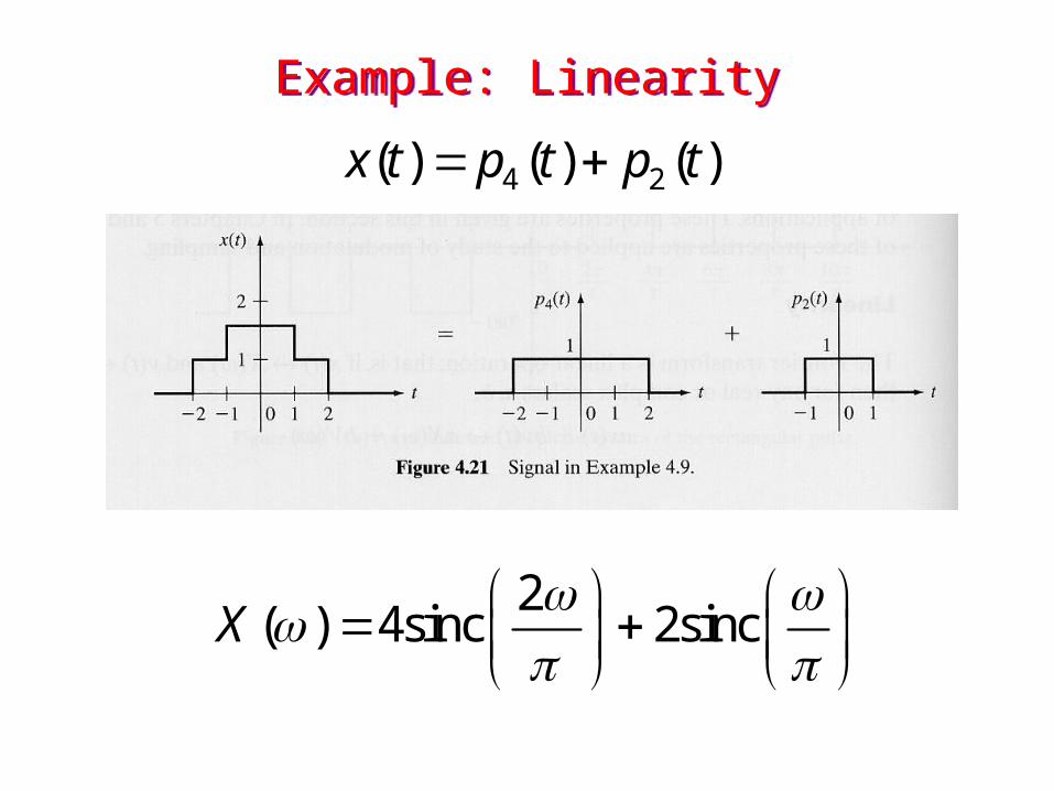
Example: LinearityExample: Linearity

4 2( ) ( ) ( )x t p t p t

2( ) 4sinc 2sincX

Example: Time ShiftExample: Time Shift

2( ) ( 1)x t p t

( ) 2sinc jX e

Example: Time ScalingExample: Time Scaling

2 ( )p t

2 (2 )p t

2sinc

sinc2

time compression frequency expansiontime expansion frequency compression

1a 0 1a

Example: Multiplication in TimeExample: Multiplication in Time

2( ) ( )x t tp t

2

sin cos sin( ) 2sinc 2 2

d dX j j j

d d

Example: Multiplication by a SinusoidExample: Multiplication by a Sinusoid

0( ) ( )cos( )x t p t t sinusoidal burst

0 01 ( ) ( )( ) sinc sinc

2 2 2X

Example: Multiplication by a Sinusoid – Cont’d


0 01 ( ) ( )( ) sinc sinc

2 2 2X

0 60 / sec

0.5

rad

Example: Multiplication in TimeExample: Multiplication in Time

2( ) ( )x t tp t

2

sin cos sin( ) 2sinc 2 2

d dX j j j

d d

Example: Multiplication by a SinusoidExample: Multiplication by a Sinusoid

0( ) ( )cos( )x t p t t sinusoidal burst

0 01 ( ) ( )( ) sinc sinc

2 2 2X



0 01 ( ) ( )( ) sinc sinc

2 2 2X

0 60 / sec

0.5

rad

Example: Integration in the Time Domain

Example: Integration in the Time Domain

2 | |( ) 1 ( )

tv t p t

( )( )

dv tx t

dt

Example: Integration in the Time Domain – Cont’d


• The Fourier transform of x(t) can be easily found to be

• Now, by using the integration property, it is

( ) sinc 2sin4 4

X j

21( ) ( ) (0) ( ) sinc

2 4V X X

j



2( ) sinc2 4

V

• Fourier transform of

• Applying the duality property

Generalized Fourier TransformGeneralized Fourier Transform

( )t

( ) 1j tt e dt

( ) 1t

( ) 1, 2 ( )x t t

generalized Fourier transformgeneralized Fourier transform of the constant signal ( ) 1,x t t

Generalized Fourier Transform of Sinusoidal Signals

Generalized Fourier Transform of Sinusoidal Signals

0 0 0cos( ) ( ) ( )t

0 0 0sin( ) ( ) ( )t j

Fourier Transform of Periodic SignalsFourier Transform of Periodic Signals

• Let x(t) be a periodic signal with period T; as such, it can be represented with its Fourier transform

• Since , it is002 ( )j te

0( ) jk tk

k

x t c e

0 2 /T

0( ) 2 ( )kk

X c k

• Since

using the integration property, it is

Fourier Transform of the Unit-Step FunctionFourier Transform of

the Unit-Step Function

( ) ( )t

u t d

1( ) ( ) ( )

t

u t dj

Common Fourier Transform PairsCommon Fourier Transform Pairs

Laplace Transform

Why use Laplace Transforms?

• Find solution to differential equation using algebra

• Relationship to Fourier Transform allows easy way to characterize systems

• No need for convolution of input and differential equation solution

• Useful with multiple processes in system

How to use Laplace

• Find differential equations that describe system

• Obtain Laplace transform• Perform algebra to solve for output or

variable of interest• Apply inverse transform to find solution

What are Laplace transforms?

j

j

st

st

dsesFj

sFLtf

dtetftfLsF

)(

2

1)}({)(

)()}({)(

1

0

• t is real, s is complex!• Inverse requires complex analysis to solve• Note “transform”: f(t) F(s), where t is integrated and s is

variable• Conversely F(s) f(t), t is variable and s is integrated• Assumes f(t) = 0 for all t < 0

Evaluating F(s) = L{f(t)}

• Hard Way – do the integral

0

0 0

)(

0

)sin()(

sin)(

1)(

)(

1)10(

1)(

1)(

dttesF

ttf

asdtedteesF

etf

ssdtesF

tf

st

tasstat

at

stlet

let

let

Evaluating F(s)=L{f(t)}- Hard Way

remember vduuvudv

)tcos(v,dt)tsin(dv

dtsedu,eu stst

0

stst

0 0

st

0

stst

dt)tcos(es)1(e

dt)tcos(es)tcos(e[dt)tsin(e ]

)tsin(v,dt)tcos(dv

dtsedu,eu stst

0

stst

0

st

0

st

0

st

dt)tsin(es)0(edt)tsin(es)tsin(e[

dt)tcos(e

]

20

st

0

st2

0 0

st2st

s1

1dt)tsin(e

1dt)tsin(e)s1(

dt)tsin(es1dt)tsin(se

let

let

Substituting, we get:

It only gets worse…

Table of selected Laplace Transforms

1s

1)s(F)t(u)tsin()t(f

1s

s)s(F)t(u)tcos()t(f

as

1)s(F)t(ue)t(f

s

1)s(F)t(u)t(f

2

2

at

More transforms

1nn

s

!n)s(F)t(ut)t(f

665

2

1

s

120

s

!5)s(F)t(ut)t(f,5n

s

!1)s(F)t(tu)t(f,1n

s

1

s

!0)s(F)t(u)t(f,0n

1)s(F)t()t(f

Note on step functions in Laplace

0

stdte)t(f)}t(f{L

0t,0)t(u

0t,1)t(u

• Unit step function definition:

• Used in conjunction with f(t) f(t)u(t) because of Laplace integral limits:

Properties of Laplace Transforms

• Linearity• Scaling in time• Time shift• “frequency” or s-plane shift• Multiplication by tn

• Integration• Differentiation

Properties: Linearity

)()()}()({ 22112211 sFcsFctfctfcL Example :

1s

1)

1s

)1s()1s((

2

1

)1s

1

1s

1(

2

1

}e{L2

1}e{L

2

1

}e2

1e

2

1{y

)}t{sinh(L

22

tt

tt

Proof :

)s(Fc)s(Fc

dte)t(fcdte)t(fc

dte)]t(fc)t(fc[

)}t(fc)t(fc{L

2211

0

st22

0

st11

st22

0

11

2211

)a

s(F

a

1)}at(f{L

Example :

22

22

2

2

s

)s

(1

)1)s(

1(

1

)}t{sin(L

Proof :

)a

s(F

a

1

due)u(fa

1

dua

1dt,

a

ut,atu

dte)at(f

)}at(f{L

a

0

u)a

s(

0

st

let

Properties: Scaling in Time

Properties: Time Shift

)s(Fe)}tt(u)tt(f{L 0st00

Example :

as

e

)}10t(ue{Ls10

)10t(a

Proof :

)s(Fedue)u(fe

due)u(f

tut,ttu

dte)tt(f

dte)tt(u)tt(f

)}tt(u)tt(f{L

00

0

0

0

st

0

sust

t

0

)tu(s

00

t

st0

0

st00

00

let

Properties: S-plane (frequency) shift

)as(F)}t(fe{L at

Example :

22

at

)as(

)}tsin(e{L

Proof :

)as(F

dte)t(f

dte)t(fe

)}t(fe{L

0

t)as(

0

stat

at

Properties: Multiplication by tn

)s(Fds

d)1()}t(ft{L

n

nnn

Example :

1n

n

nn

n

s

!n

)s

1(

ds

d)1(

)}t(ut{L

Proof :

)s(Fs

)1(dte)t(fs

)1(

dtes

)t(f)1(

dtet)t(f

dte)t(ft)}t(ft{L

n

nn

0

stn

nn

0

stn

nn

0

stn

0

stnn

The “D” Operator

1. Differentiation shorthand

2. Integration shorthand)t(f

dt

d)t(fD

dt

)t(df)t(Df

2

22

)t(f)t(Dg

dt)t(f)t(gt

)t(fD)t(g

dt)t(f)t(g

1a

t

a

if

then then

if

Properties: Integrals

s

)s(F)}t(fD{L 1

0

Example :

)}t{sin(L1s

1)

1s

s)(

s

1(

)}tcos(D{L

22

10

Proof :

let

stst

0

st

10

es

1v,dtedv

dt)t(fdu),t(gu

dte)t(g)}t{sin(L

)t(fD)t(g

t

0

st0

st

dt)t(f)t(g

s

)s(Fdte)t(f

s

1]e)t(g

s

1[

0

)()( dtetft st If t=0, g(t)=0

for so

slower than

0

)()( tgdttf 0 ste

Properties: Derivatives(this is the big one)

)0(f)s(sF)}t(Df{L Example :

)}tsin({L1s

11s

)1s(s

11s

s

)0(f1s

s

)}tcos(D{L

2

2

22

2

2

2

2

Proof :

)s(sF)0(f

dte)t(fs)]t(fe[

)t(fv,dt)t(fdt

ddv

sedu,eu

dte)t(fdt

d)}t(Df{L

0

st0

st

stst

0

st

let

The Inverse Laplace Transform

Inverse Laplace Transforms

Background:

To find the inverse Laplace transform we use transform pairsalong with partial fraction expansion:

F(s) can be written as;

)(

)()(

sQ

sPsF

Where P(s) & Q(s) are polynomials in the Laplace variable, s.We assume the order of Q(s) P(s), in order to be in properform. If F(s) is not in proper form we use long division and divide Q(s) into P(s) until we get a remaining ratio of polynomialsthat are in proper form.


Background:There are three cases to consider in doing the partial fraction expansion of F(s).

Case 1: F(s) has all non repeated simple roots.

n

n

ps

k

ps

k

ps

ksF

...)(

2

2

1

1

Case 2: F(s) has complex poles:

...)))()((

)()(

*11

1

1

js

k

js

k

jsjssQ

sPsF

Case 3: F(s) has repeated poles.

)(

)(...

)(...

)())((

)()(

1

1

1

12

1

12

1

11

11

1

sQ

sP

ps

k

ps

k

ps

k

pssQ

sPsF

rr

r

(expanded)

(expanded)


Case 1: Illustration:

Given:

)10()4()1()10)(4)(1(

)2(4)( 321

s

A

s

A

s

A

sss

ssF

274)10)(4)(1(

)2(4)1(| 11

ssss

ssA 94

)10)(4)(1(

)2(4)4(| 42

ssss

ssA

2716)10)(4)(1(

)2(4)10(| 103

ssss

ssA

)()2716()94()274()( 104 tueeetf ttt

Find A1, A2, A3 from Heavyside


Case 3: Repeated roots.

When we have repeated roots we find the coefficients of the terms as follows:

|111

)()(1 psr

sFpsds

dk r

|121

)()(!2 12

2

psrsFps

ds

dk r

|11

)()()!( 1 psj

sFpsdsjr

dk r

jr

jr


Case 3: Repeated roots. Example

2

1

1

2211

2 )3()3()3(

)1()(

K

K

A

s

K

s

K

s

A

ss

ssF

)(____________________)( 33 tuteetf tt ? ? ?


Complex Roots: An Example.

For the given F(s) find f(t)

o

jj

j

jss

sK

ss

sA

js

K

js

K

s

AsF

jsjss

s

sss

ssF

js

s

10832.0)2)(2(

12

)2(

)1(

5

1

)54(

)1(

22)(

)2)(2(

)1(

)54(

)1()(

|

|

2|1

0|

11

2

2

*


Complex Roots: An Example. (continued)

We then have;

jsjsssF

oo

2

10832.0

2

10832.02.0)(

Recalling the form of the inverse for complex roots;

)(108cos(64.02.0)( 2 tutetf ot

Fourier Series. Introduction Decompose a periodic input signal into primitive periodic components. A...

Documents

Transcript of Fourier Series. Introduction Decompose a periodic input signal into primitive periodic components. A...