Fourier Series

Chapter 1

Fourier Series

Jean Baptiste Joseph Fourier (1768-1830) was a French mathematician, physi-cist and engineer, and the founder of Fourier analysis. In 1822 he made theclaim, seemingly preposterous at the time, that any function of t, continuousor discontinuous, could be represented as a linear combination of functionssinnt. This was a dramatic distinction from Taylor series. While not strictlytrue in fact, this claim was true in spirit and it led to the modern theory ofFourier analysis with wide applications to science and engineering.

1.1 Definitions, Real and complex Fourier se-

ries

We have observed that the functions en(t) = eint/√

2π, n = 0,±1,±2, · · ·form an ON set in the Hilbert space L2[0, 2π] of square-integrable functionson the interval [0, 2π]. In fact we shall show that these functions form an ONbasis. Here the inner product is

(u, v) =

∫ 2π

0

u(t)v(t) dt, u, v ∈ L2[0, 2π].

We will study this ON set and the completeness and convergence of expan-sions in the basis, both pointwise and in the norm. Before we get started, itis convenient to assume that L2[0, 2π] consists of square-integrable functionson the unit circle, rather than on an interval of the real line. Thus we willreplace every function f(t) on the interval [0, 2π] by a function f ∗(t) suchthat f ∗(0) = f ∗(2π) and f ∗(t) = f(t) for 0 ≤ t < 2π. Then we will extend

1

f ∗ to all −∞ < t <∞ by requiring periodicity: f ∗(t+2π) = f ∗(t). This willnot affect the values of any integrals over the interval [0, 2π], though it maychange the value of f at one point. Thus, from now on our functions will beassumed 2π − periodic. One reason for this assumption is the

Lemma 1 Suppose F is 2π − periodic and integrable. Then for any realnumber a ∫ 2π+a

a

F (t)dt =

∫ 2π

0

F (t)dt.

Proof Each side of the identity is just the integral of F over one period.For an analytic proof, note that∫ 2π

0

F (t)dt =

∫ a

0

F (t)dt+

∫ 2π

a

F (t)dt =

∫ a

0

F (t+ 2π)dt+

∫ 2π

a

F (t)dt

=

∫ 2π+a

2π

F (t)dt+

∫ 2π

a

F (t)dt =

∫ 2π

a

F (t)dt+

∫ 2π+a

2π

F (t)dt

=

∫ 2π+a

a

F (t)dt.

2

Thus we can transfer all our integrals to any interval of length 2π withoutaltering the results.

Exercise 1 Let G(a) =∫ 2π+a

aF (t)dt and give a new proof of of Lemma 1

based on a computation of the derivative G′(a).

For students who don’t have a background in complex variable theory wewill define the complex exponential in terms of real sines and cosines, andderive some of its basic properties directly. Let z = x + iy be a complexnumber, where x and y are real. (Here and in all that follows, i =

√−1.)

Then z = x− iy.

Definition 1 ez = exp(x)(cos y + i sin y)

Lemma 2 Properties of the complex exponential:

• ez1ez2 = ez1+z2

• |ez| = exp(x)

2

• ez = ez = exp(x)(cos y − i sin y).

Exercise 2 Verify lemma 2. You will need the addition formula for sinesand cosines.

Simple consequences for the basis functions en(t) = eint/√

2π, n = 0,±1,±2, · · ·where t is real, are given by

Lemma 3 Properties of eint:

• ein(t+2π) = eint

• |eint| = 1

• eint = e−int

• eimteint = ei(m+n)t

• e0 = 1

• ddteint = ineint.

Lemma 4 (en, em) = δnm.

Proof If n 6= m then

(en, em) =1

2π

∫ 2π

0

ei(n−m)tdt =1

2π

ei(n−m)t

i(n−m)|2π0 = 0.

If n = m then (en, em) = 12π

∫ 2π

01 dt = 1. 2

Since {en} is an ON set, we can project any f ∈ L2[0, 2π] on the closedsubspace generated by this set to get the Fourier expansion

f(t) ∼∞∑

n=−∞

(f, en)en(t),

or

f(t) ∼∞∑

n=−∞

cneint, cn =

1

2π

∫ 2π

0

f(t)e−intdt. (1.1.1)

This is the complex version of Fourier series. (For now the ∼ just denotesthat the right-hand side is the Fourier series of the left-hand side. In what

3

sense the Fourier series represents the function is a matter to be resolved.)From our study of Hilbert spaces we already know that Bessel’s inequalityholds: (f, f) ≥

∑∞n=−∞ |(f, en)|2 or

1

2π

∫ 2π

0

|f(t)|2dt ≥∞∑

n=−∞

|cn|2. (1.1.2)

An immediate consequence is the Riemann-Lebesgue Lemma.

Lemma 5 (Riemann-Lebesgue, weak form) lim|n|→∞∫ 2π

0f(t)e−intdt = 0.

Thus, as |n| gets large the Fourier coefficients go to 0.If f is a real-valued function then cn = c−n for all n. If we set

cn =an − ibn

2, n = 0, 1, 2, · · ·

c−n =an + ibn

2, n = 1, 2, · · ·

and rearrange terms, we get the real version of Fourier series:

f(t) ∼ a0

2+∞∑n=1

(an cosnt+ bn sinnt), (1.1.3)

an =1

π

∫ 2π

0

f(t) cosnt dt bn =1

π

∫ 2π

0

f(t) sinnt dt

with Bessel inequality

1

π

∫ 2π

0

|f(t)|2dt ≥ |a0|2

2+∞∑n=1

(|an|2 + |bn|2),

and Riemann-Lebesgue Lemma

limn→∞

∫ 2π

0

f(t) cos(nt)dt = limn→∞

∫ 2π

0

f(t) sin(nt)dt = 0.

Remark: The set { 1√2π, 1√

πcosnt, 1√

πsinnt} for n = 1, 2, · · · is also ON in

L2[0, 2π], as is easy to check, so (1.1.3) is the correct Fourier expansion inthis basis for complex functions f(t), as well as real functions.

Later we will prove the following basic results:

4

Theorem 1 Parseval’s equality. Let f ∈ L2[0, 2π]. Then

(f, f) =∞∑

n=−∞

|(f, en)|2.

In terms of the complex and real versions of Fourier series this reads

1

2π

∫ 2π

0

|f(t)|2dt =∞∑

n=−∞

|cn|2 (1.1.4)

or1

π

∫ 2π

0

|f(t)|2dt =|a0|2

2+∞∑n=1

(|an|2 + |bn|2).

Let f ∈ L2[0, 2π] and remember that we are assuming that all suchfunctions satisfy f(t + 2π) = f(t). We say that f is piecewise continu-ous on [0, 2π] if it is continuous except for a finite number of discontinu-ities. Furthermore, at each t the limits f(t + 0) = limh→0,h>0 f(t + h) andf(t−0) = limh→0,h>0 f(t−h) exist. NOTE: At a point t of continuity of f we

have f(t+0) = f(t−0), whereas at a point of discontinuity f(t+0) 6= f(t−0)and f(t+ 0)− f(t− 0) is the magnitude of the jump discontinuity.

Theorem 2 Suppose

• f(t) is periodic with period 2π.

• f(t) is piecewise continuous on [0, 2π].

• f ′(t) is piecewise continuous on [0, 2π].

Then the Fourier series of f(t) converges to f(t+0)+f(t−0)2

at each point t.

1.2 Examples

We will use the real version of Fourier series for these examples. The trans-formation to the complex version is elementary.

5

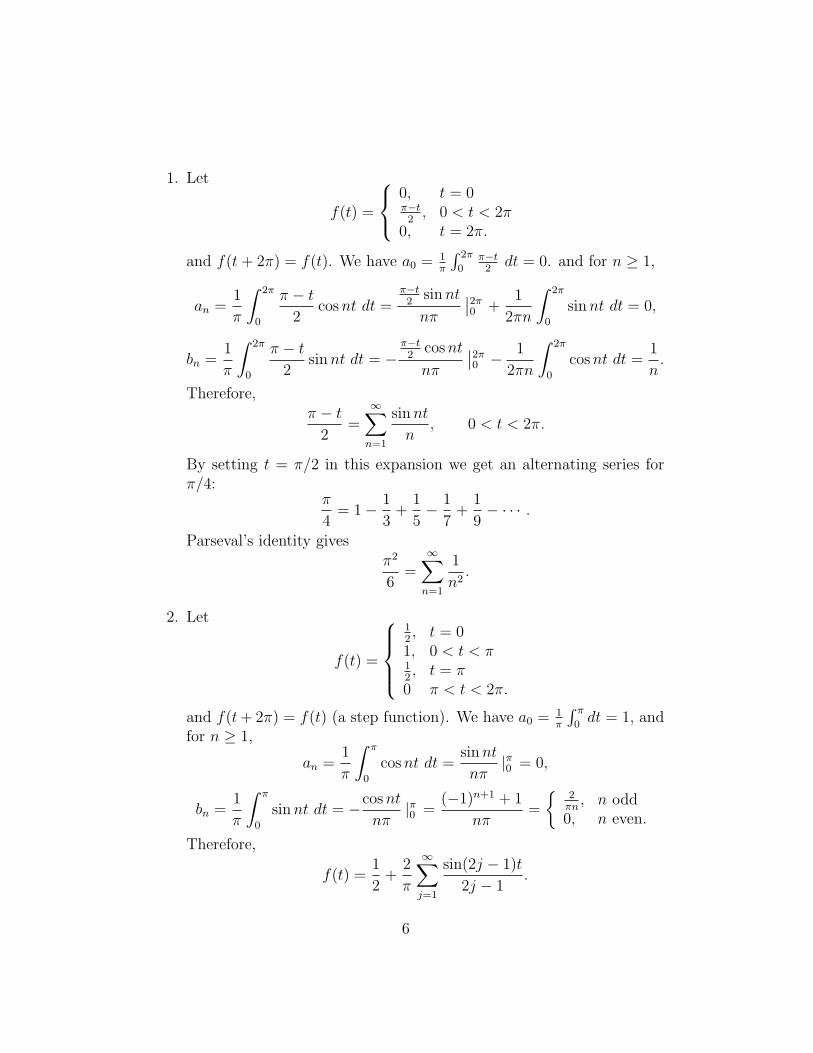
1. Let

f(t) =

0, t = 0π−t2, 0 < t < 2π

0, t = 2π.

and f(t+ 2π) = f(t). We have a0 = 1π

∫ 2π

0π−t2dt = 0. and for n ≥ 1,

an =1

π

∫ 2π

0

π − t2

cosnt dt =π−t2

sinnt

nπ

∣∣2π0 +

1

2πn

∫ 2π

0

sinnt dt = 0,

bn =1

π

∫ 2π

0

π − t2

sinnt dt = −π−t2

cosnt

nπ

∣∣2π0 −

1

2πn

∫ 2π

0

cosnt dt =1

n.

Therefore,π − t

2=∞∑n=1

sinnt

n, 0 < t < 2π.

By setting t = π/2 in this expansion we get an alternating series forπ/4:

π

4= 1− 1

3+

1

5− 1

7+

1

9− · · · .

Parseval’s identity givesπ2

6=∞∑n=1

1

n2.

2. Let

f(t) =

12, t = 0

1, 0 < t < π12, t = π

0 π < t < 2π.

and f(t+ 2π) = f(t) (a step function). We have a0 = 1π

∫ π0dt = 1, and

for n ≥ 1,

an =1

π

∫ π

0

cosnt dt =sinnt

nπ|π0 = 0,

bn =1

π

∫ π

0

sinnt dt = −cosnt

nπ|π0 =

(−1)n+1 + 1

nπ=

{2πn, n odd

0, n even.

Therefore,

f(t) =1

2+

2

π

∞∑j=1

sin(2j − 1)t

2j − 1.

6

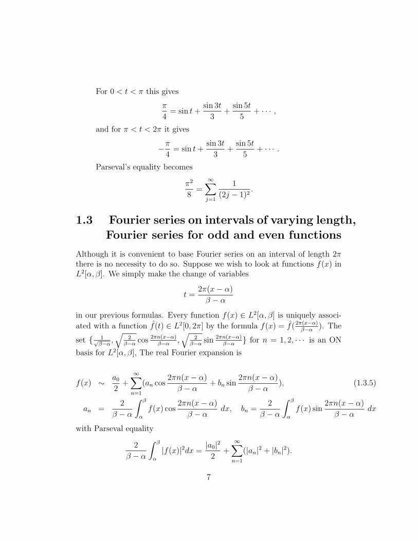
For 0 < t < π this gives

π

4= sin t+

sin 3t

3+

sin 5t

5+ · · · ,

and for π < t < 2π it gives

−π4

= sin t+sin 3t

3+

sin 5t

5+ · · · .

Parseval’s equality becomes

π2

8=∞∑j=1

1

(2j − 1)2.

1.3 Fourier series on intervals of varying length,

Fourier series for odd and even functions

Although it is convenient to base Fourier series on an interval of length 2πthere is no necessity to do so. Suppose we wish to look at functions f(x) inL2[α, β]. We simply make the change of variables

t =2π(x− α)

β − α

in our previous formulas. Every function f(x) ∈ L2[α, β] is uniquely associ-

ated with a function f(t) ∈ L2[0, 2π] by the formula f(x) = f(2π(x−α)β−α ). The

set { 1√β−α ,

√2

β−α cos 2πn(x−α)β−α ,

√2

β−α sin 2πn(x−α)β−α } for n = 1, 2, · · · is an ON

basis for L2[α, β], The real Fourier expansion is

f(x) ∼ a0

2+∞∑n=1

(an cos2πn(x− α)

β − α+ bn sin

2πn(x− α)

β − α), (1.3.5)

an =2

β − α

∫ β

α

f(x) cos2πn(x− α)

β − αdx, bn =

2

β − α

∫ β

α

f(x) sin2πn(x− α)

β − αdx

with Parseval equality

2

β − α

∫ β

α

|f(x)|2dx =|a0|2

2+∞∑n=1

(|an|2 + |bn|2).

7

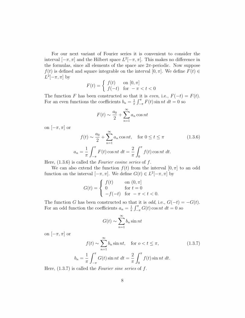
For our next variant of Fourier series it is convenient to consider theinterval [−π, π] and the Hilbert space L2[−π, π]. This makes no difference inthe formulas, since all elements of the space are 2π-periodic. Now supposef(t) is defined and square integrable on the interval [0, π]. We define F (t) ∈L2[−π, π] by

F (t) =

{f(t) on [0, π]f(−t) for − π < t < 0

The function F has been constructed so that it is even, i.e., F (−t) = F (t).For an even functions the coefficients bn = 1

π

∫ π−π F (t) sinnt dt = 0 so

F (t) ∼ a0

2+∞∑n=1

an cosnt

on [−π, π] or

f(t) ∼ a0

2+∞∑n=1

an cosnt, for 0 ≤ t ≤ π (1.3.6)

an =1

π

∫ π

−πF (t) cosnt dt =

2

π

∫ π

0

f(t) cosnt dt.

Here, (1.3.6) is called the Fourier cosine series of f .We can also extend the function f(t) from the interval [0, π] to an odd

function on the interval [−π, π]. We define G(t) ∈ L2[−π, π] by

G(t) =

f(t) on (0, π]0 for t = 0−f(−t) for − π < t < 0.

The function G has been constructed so that it is odd, i.e., G(−t) = −G(t).For an odd function the coefficients an = 1

π

∫ π−π G(t) cosnt dt = 0 so

G(t) ∼∞∑n=1

bn sinnt

on [−π, π] or

f(t) ∼∞∑n=1

bn sinnt, for o < t ≤ π, (1.3.7)

bn =1

π

∫ π

−πG(t) sinnt dt =

2

π

∫ π

0

f(t) sinnt dt.

Here, (1.3.7) is called the Fourier sine series of f .

8

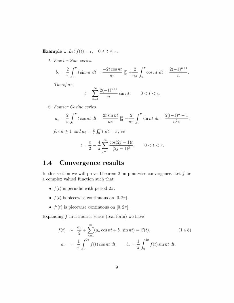
Example 1 Let f(t) = t, 0 ≤ t ≤ π.

1. Fourier Sine series.

bn =2

π

∫ π

0

t sinnt dt =−2t cosnt

nπ|π0 +

2

nπ

∫ π

0

cosnt dt =2(−1)n+1

n.

Therefore,

t =∞∑n=1

2(−1)n+1

nsinnt, 0 < t < π.

2. Fourier Cosine series.

an =2

π

∫ π

0

t cosnt dt =2t sinnt

nπ|π0 −

2

nπ

∫ π

0

sinnt dt =2[(−1)n − 1

n2π,

for n ≥ 1 and a0 = 2π

∫ π0t dt = π, so

t =π

2− 4

π

∞∑j=1

cos(2j − 1)t

(2j − 1)2, 0 < t < π.

1.4 Convergence results

In this section we will prove Theorem 2 on pointwise convergence. Let f bea complex valued function such that




Expanding f in a Fourier series (real form) we have

f(t) ∼ a0

2+∞∑n=1

(an cosnt+ bn sinnt) = S(t), (1.4.8)

an =1

π

∫ 2π

0

f(t) cosnt dt, bn =1

π

∫ 2π

0

f(t) sinnt dt.

9

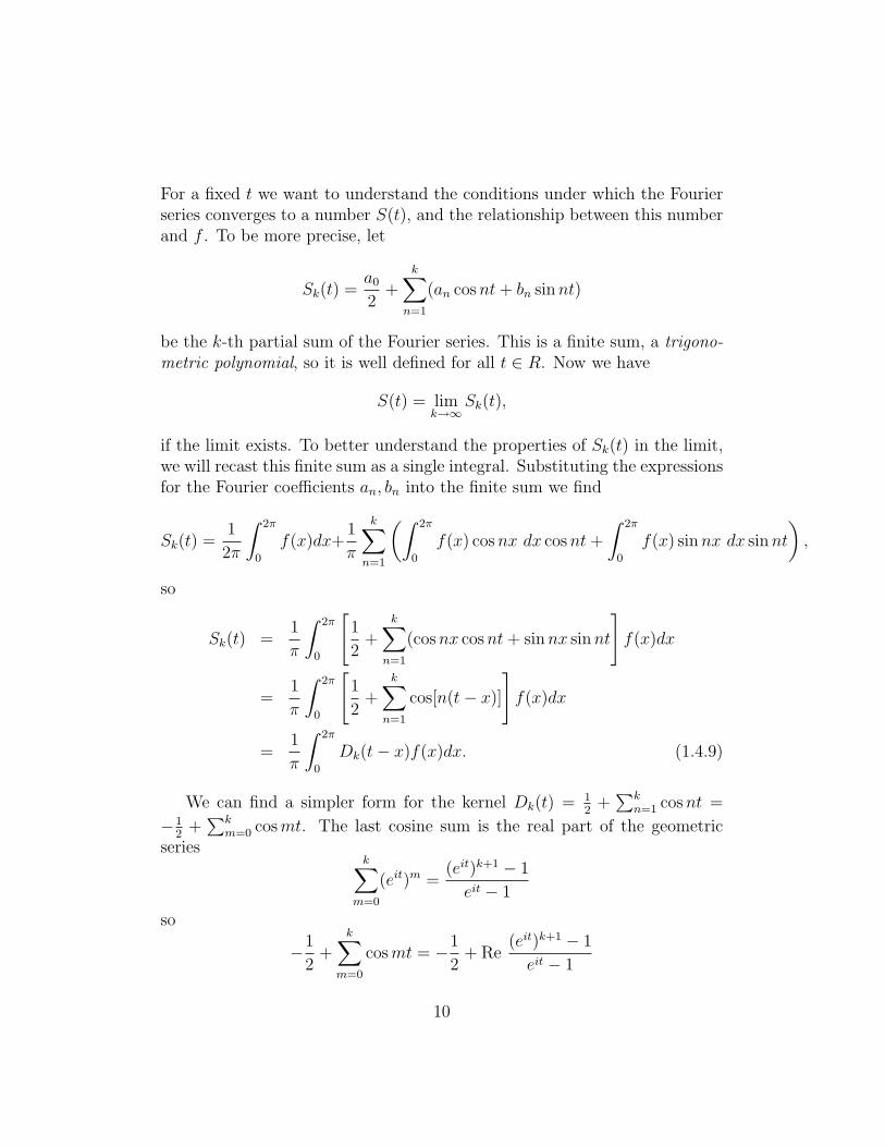
For a fixed t we want to understand the conditions under which the Fourierseries converges to a number S(t), and the relationship between this numberand f . To be more precise, let

Sk(t) =a0

2+

k∑n=1

(an cosnt+ bn sinnt)

be the k-th partial sum of the Fourier series. This is a finite sum, a trigono-metric polynomial, so it is well defined for all t ∈ R. Now we have

S(t) = limk→∞

Sk(t),

if the limit exists. To better understand the properties of Sk(t) in the limit,we will recast this finite sum as a single integral. Substituting the expressionsfor the Fourier coefficients an, bn into the finite sum we find

Sk(t) =1

2π

∫ 2π

0

f(x)dx+1

π

k∑n=1

(∫ 2π

0

f(x) cosnx dx cosnt+

∫ 2π

0

f(x) sinnx dx sinnt

),

so

Sk(t) =1

π

∫ 2π

0

[1

2+

k∑n=1

(cosnx cosnt+ sinnx sinnt

]f(x)dx

=1

π

∫ 2π

0

[1

2+

k∑n=1

cos[n(t− x)]

]f(x)dx

=1

π

∫ 2π

0

Dk(t− x)f(x)dx. (1.4.9)

We can find a simpler form for the kernel Dk(t) = 12

+∑k

n=1 cosnt =

−12

+∑k

m=0 cosmt. The last cosine sum is the real part of the geometricseries

k∑m=0

(eit)m =(eit)k+1 − 1

eit − 1

so

−1

2+

k∑m=0

cosmt = −1

2+ Re

(eit)k+1 − 1

eit − 1

10

= Re(eit)k+1 − 1

2eit − 1

2

eit − 1= Re

12(e−iu/2eiu/2 − ei(k+1/2)u

e−iu/2 − eiu/2

= Resin(k + 1/2)u+ i(cosu/2− cos(k + 1/2)u)

2 sinu/2.

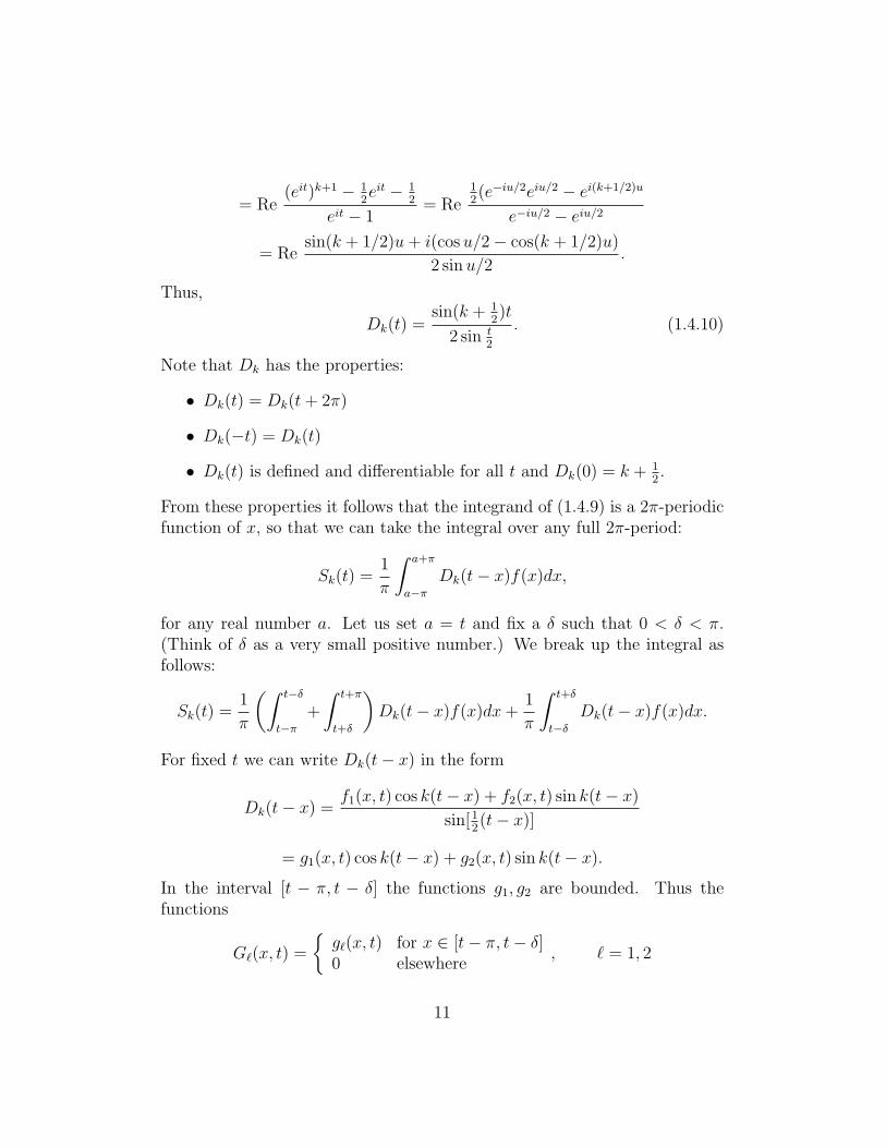
Thus,

Dk(t) =sin(k + 1

2)t

2 sin t2

. (1.4.10)

Note that Dk has the properties:

• Dk(t) = Dk(t+ 2π)

• Dk(−t) = Dk(t)

• Dk(t) is defined and differentiable for all t and Dk(0) = k + 12.

From these properties it follows that the integrand of (1.4.9) is a 2π-periodicfunction of x, so that we can take the integral over any full 2π-period:

Sk(t) =1

π

∫ a+π

a−πDk(t− x)f(x)dx,

for any real number a. Let us set a = t and fix a δ such that 0 < δ < π.(Think of δ as a very small positive number.) We break up the integral asfollows:

Sk(t) =1

π

(∫ t−δ

t−π+

∫ t+π

t+δ

)Dk(t− x)f(x)dx+

1

π

∫ t+δ

t−δDk(t− x)f(x)dx.

For fixed t we can write Dk(t− x) in the form

Dk(t− x) =f1(x, t) cos k(t− x) + f2(x, t) sin k(t− x)

sin[12(t− x)]

= g1(x, t) cos k(t− x) + g2(x, t) sin k(t− x).

In the interval [t − π, t − δ] the functions g1, g2 are bounded. Thus thefunctions

G`(x, t) =

{g`(x, t) for x ∈ [t− π, t− δ]0 elsewhere

, ` = 1, 2

11

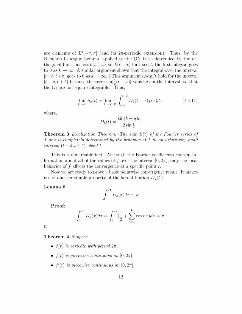
are elements of L2[−π, π] (and its 2π-periodic extension). Thus, by theRiemann-Lebesgue Lemma, applied to the ON basis determied by the or-thogonal functions cos k(t− x), sin k(t− x) for fixed t, the first integral goesto 0 as k →∞. A similar argument shows that the integral over the interval[t+δ, t+π] goes to 0 as k →∞. [ This argument doesn’t hold for the interval[t − δ, t + δ] because the term sin[1

2(t − x)] vanishes in the interval, so that

the G` are not square integrable.] Thus,

limk→∞

Sk(t) = limk→∞

1

π

∫ t+δ

t−δDk(t− x)f(x)dx, (1.4.11)

where,

Dk(t) =sin(k + 1

2)t

2 sin t2

.

Theorem 3 Localization Theorem. The sum S(t) of the Fourier series off at t is completely determined by the behavior of f in an arbitrarily smallinterval (t− δ, t+ δ) about t.

This is a remarkable fact! Although the Fourier coefficients contain in-formation about all of the values of f over the interval [0, 2π), only the localbehavior of f affects the convergence at a specific point t.

Now we are ready to prove a basic pointwise convergence result. It makesuse of another simple property of the kernal funtion Dk(t):

Lemma 6 ∫ 2π

0

Dk(x)dx = π

Proof; ∫ 2π

0

Dk(x)dx =

∫ 2π

0

(1

2+

k∑n=1

cosnx)dx = π.

2

Theorem 4 Suppose




12

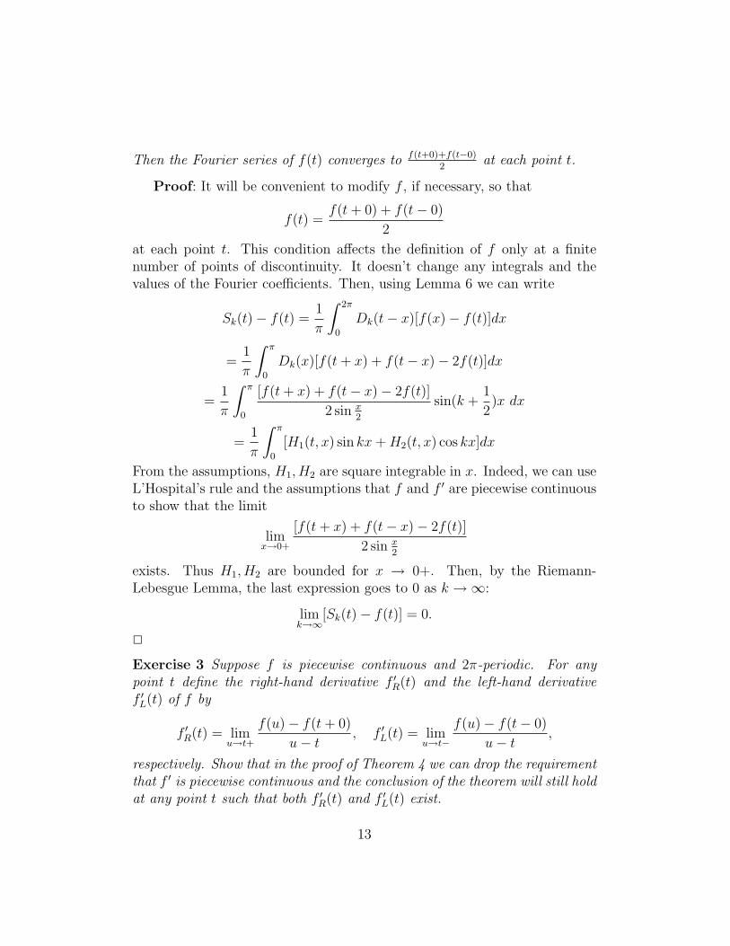
Then the Fourier series of f(t) converges to f(t+0)+f(t−0)2

at each point t.

Proof: It will be convenient to modify f , if necessary, so that

f(t) =f(t+ 0) + f(t− 0)

2

at each point t. This condition affects the definition of f only at a finitenumber of points of discontinuity. It doesn’t change any integrals and thevalues of the Fourier coefficients. Then, using Lemma 6 we can write

Sk(t)− f(t) =1

π

∫ 2π

0

Dk(t− x)[f(x)− f(t)]dx

=1

π

∫ π

0

Dk(x)[f(t+ x) + f(t− x)− 2f(t)]dx

=1

π

∫ π

0

[f(t+ x) + f(t− x)− 2f(t)]

2 sin x2

sin(k +1

2)x dx

=1

π

∫ π

0

[H1(t, x) sin kx+H2(t, x) cos kx]dx

From the assumptions, H1, H2 are square integrable in x. Indeed, we can useL’Hospital’s rule and the assumptions that f and f ′ are piecewise continuousto show that the limit

limx→0+

[f(t+ x) + f(t− x)− 2f(t)]

2 sin x2

exists. Thus H1, H2 are bounded for x → 0+. Then, by the Riemann-Lebesgue Lemma, the last expression goes to 0 as k →∞:

limk→∞

[Sk(t)− f(t)] = 0.

2

Exercise 3 Suppose f is piecewise continuous and 2π-periodic. For anypoint t define the right-hand derivative f ′R(t) and the left-hand derivativef ′L(t) of f by

f ′R(t) = limu→t+

f(u)− f(t+ 0)

u− t, f ′L(t) = lim

u→t−

f(u)− f(t− 0)

u− t,

respectively. Show that in the proof of Theorem 4 we can drop the requirementthat f ′ is piecewise continuous and the conclusion of the theorem will still holdat any point t such that both f ′R(t) and f ′L(t) exist.

13

Exercise 4 Show that if f and f ′ are piecewise continuous then for any pointt we have f ′(t + 0) = f ′R(t) and f ′(t− 0) = f ′L(t). Hint: By the mean valuetheorem of calculus, for u > t and u sufficiently close to t there is a point csuch that t < c < u and

f(u)− f(t+ 0)

u− t= f ′(c).

Exercise 5 Let

f(t) =

{t2 sin(1

t) for t 6= 0

0 for t = 0.

Show that f is continuous for all t and that f ′R(0) = f ′L(0) = 0. Show thatf ′(t + 0 and f ′(t − 0) do not exist for t = 0. Hence, argue that f ′ is not apiecewise continuous function. This shows that the result of Exercise 3 is atrue strengthening of Theorem 4.

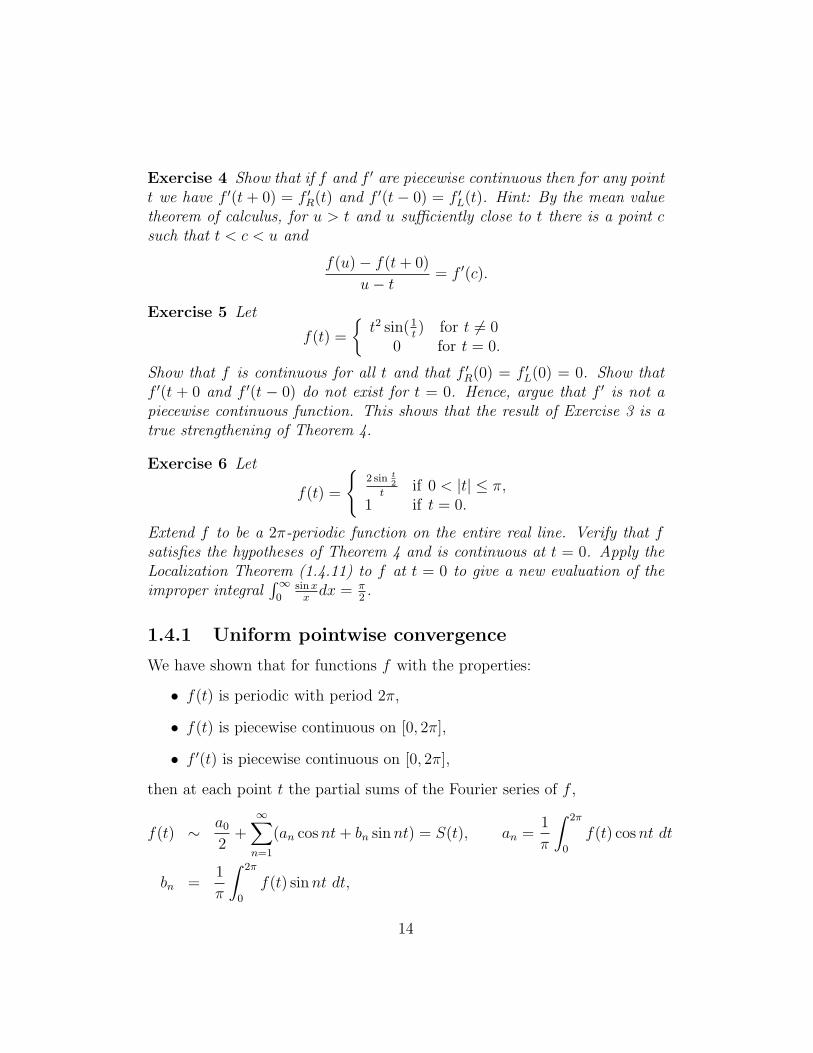
Exercise 6 Let

f(t) =

{2 sin t

2

tif 0 < |t| ≤ π,

1 if t = 0.

Extend f to be a 2π-periodic function on the entire real line. Verify that fsatisfies the hypotheses of Theorem 4 and is continuous at t = 0. Apply theLocalization Theorem (1.4.11) to f at t = 0 to give a new evaluation of theimproper integral

∫∞0

sinxxdx = π

2.

1.4.1 Uniform pointwise convergence

We have shown that for functions f with the properties:

• f(t) is periodic with period 2π,

• f(t) is piecewise continuous on [0, 2π],

• f ′(t) is piecewise continuous on [0, 2π],

then at each point t the partial sums of the Fourier series of f ,

f(t) ∼ a0

2+∞∑n=1

(an cosnt+ bn sinnt) = S(t), an =1

π

∫ 2π

0

f(t) cosnt dt

bn =1

π

∫ 2π

0

f(t) sinnt dt,

14

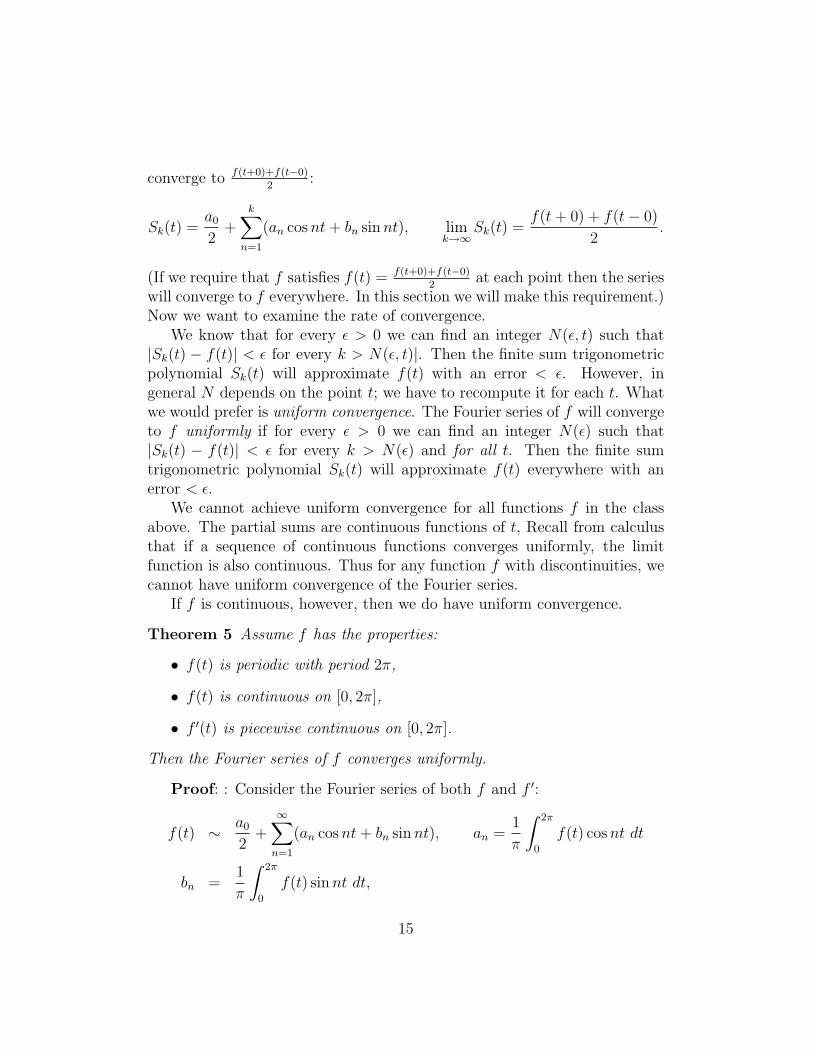
converge to f(t+0)+f(t−0)2

:

Sk(t) =a0

2+

k∑n=1

(an cosnt+ bn sinnt), limk→∞

Sk(t) =f(t+ 0) + f(t− 0)

2.

(If we require that f satisfies f(t) = f(t+0)+f(t−0)2

at each point then the serieswill converge to f everywhere. In this section we will make this requirement.)Now we want to examine the rate of convergence.

We know that for every ε > 0 we can find an integer N(ε, t) such that|Sk(t) − f(t)| < ε for every k > N(ε, t)|. Then the finite sum trigonometricpolynomial Sk(t) will approximate f(t) with an error < ε. However, ingeneral N depends on the point t; we have to recompute it for each t. Whatwe would prefer is uniform convergence. The Fourier series of f will convergeto f uniformly if for every ε > 0 we can find an integer N(ε) such that|Sk(t) − f(t)| < ε for every k > N(ε) and for all t. Then the finite sumtrigonometric polynomial Sk(t) will approximate f(t) everywhere with anerror < ε.

We cannot achieve uniform convergence for all functions f in the classabove. The partial sums are continuous functions of t, Recall from calculusthat if a sequence of continuous functions converges uniformly, the limitfunction is also continuous. Thus for any function f with discontinuities, wecannot have uniform convergence of the Fourier series.

If f is continuous, however, then we do have uniform convergence.

Theorem 5 Assume f has the properties:

• f(t) is periodic with period 2π,

• f(t) is continuous on [0, 2π],


Then the Fourier series of f converges uniformly.

Proof: : Consider the Fourier series of both f and f ′:

f(t) ∼ a0

2+∞∑n=1

(an cosnt+ bn sinnt), an =1

π

∫ 2π

0

f(t) cosnt dt

bn =1

π

∫ 2π

0

f(t) sinnt dt,

15

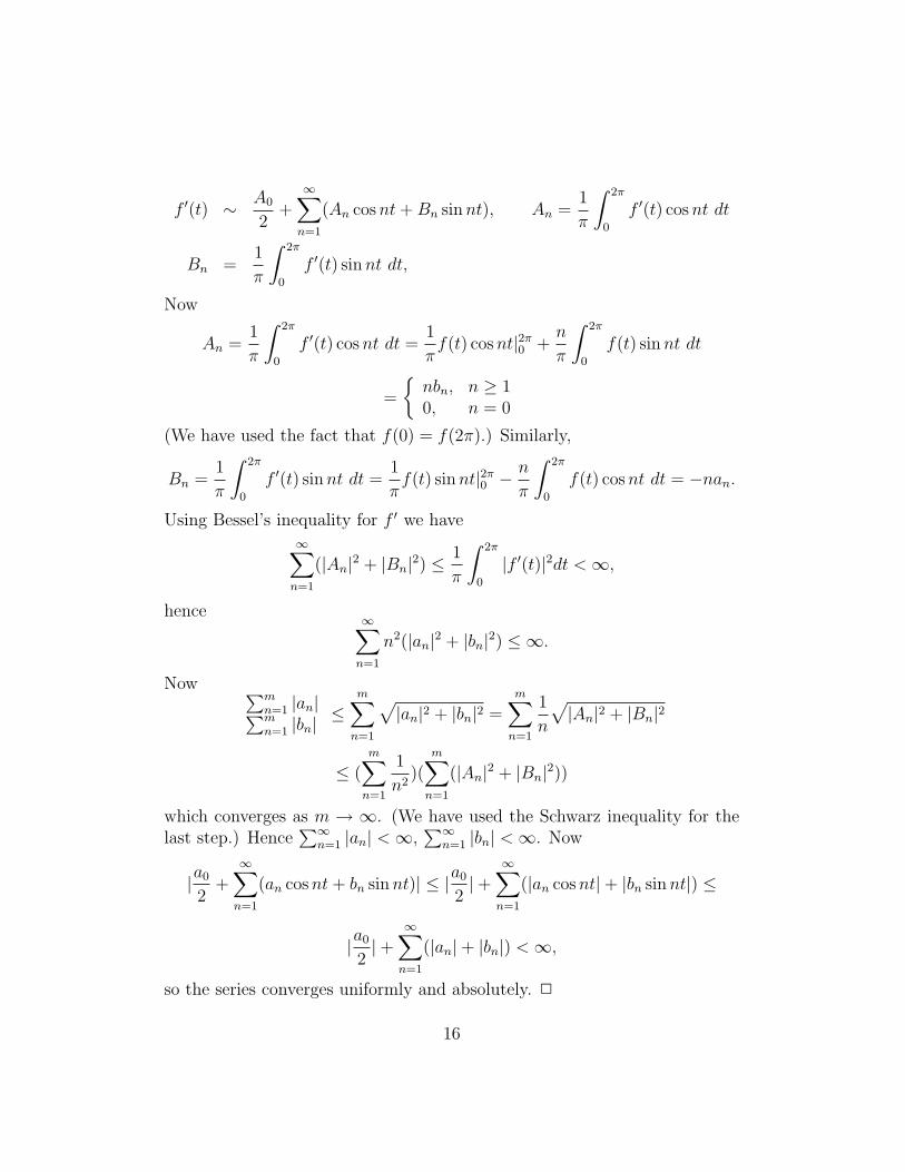
f ′(t) ∼ A0

2+∞∑n=1

(An cosnt+Bn sinnt), An =1

π

∫ 2π

0

f ′(t) cosnt dt

Bn =1

π

∫ 2π

0

f ′(t) sinnt dt,

Now

An =1

π

∫ 2π

0

f ′(t) cosnt dt =1

πf(t) cosnt|2π0 +

n

π

∫ 2π

0

f(t) sinnt dt

=

{nbn, n ≥ 10, n = 0

(We have used the fact that f(0) = f(2π).) Similarly,

Bn =1

π

∫ 2π

0

f ′(t) sinnt dt =1

πf(t) sinnt|2π0 −

n

π

∫ 2π

0

f(t) cosnt dt = −nan.

Using Bessel’s inequality for f ′ we have

∞∑n=1

(|An|2 + |Bn|2) ≤1

π

∫ 2π

0

|f ′(t)|2dt <∞,

hence∞∑n=1

n2(|an|2 + |bn|2) ≤ ∞.

Now ∑mn=1 |an|∑mn=1 |bn|

≤m∑n=1

√|an|2 + |bn|2 =

m∑n=1

1

n

√|An|2 + |Bn|2

≤ (m∑n=1

1

n2)(

m∑n=1

(|An|2 + |Bn|2))

which converges as m → ∞. (We have used the Schwarz inequality for thelast step.) Hence

∑∞n=1 |an| <∞,

∑∞n=1 |bn| <∞. Now

|a0

2+∞∑n=1

(an cosnt+ bn sinnt)| ≤ |a0

2|+

∞∑n=1

(|an cosnt|+ |bn sinnt|) ≤

|a0

2|+

∞∑n=1

(|an|+ |bn|) <∞,

so the series converges uniformly and absolutely. 2

16

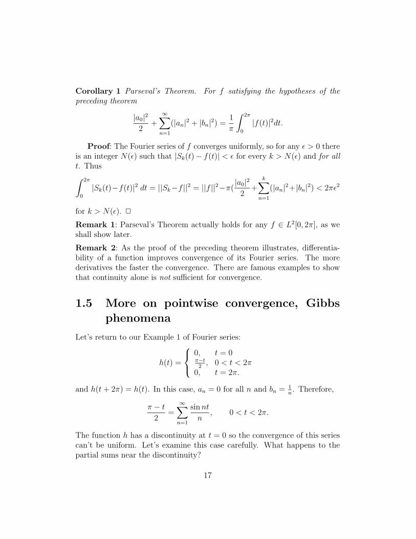
Corollary 1 Parseval’s Theorem. For f satisfying the hypotheses of thepreceding theorem

|a0|2

2+∞∑n=1

(|an|2 + |bn|2) =1

π

∫ 2π

0

|f(t)|2dt.

Proof: The Fourier series of f converges uniformly, so for any ε > 0 thereis an integer N(ε) such that |Sk(t)− f(t)| < ε for every k > N(ε) and for allt. Thus∫ 2π

0

|Sk(t)−f(t)|2 dt = ||Sk−f ||2 = ||f ||2−π(|a0|2

2+

k∑n=1

(|an|2+|bn|2) < 2πε2

for k > N(ε). 2

Remark 1: Parseval’s Theorem actually holds for any f ∈ L2[0, 2π], as weshall show later.

Remark 2: As the proof of the preceding theorem illustrates, differentia-bility of a function improves convergence of its Fourier series. The morederivatives the faster the convergence. There are famous examples to showthat continuity alone is not sufficient for convergence.

1.5 More on pointwise convergence, Gibbs

phenomena

Let’s return to our Example 1 of Fourier series:

h(t) =

0, t = 0π−t2, 0 < t < 2π

0, t = 2π.

and h(t+ 2π) = h(t). In this case, an = 0 for all n and bn = 1n. Therefore,

π − t2

=∞∑n=1

sinnt

n, 0 < t < 2π.

The function h has a discontinuity at t = 0 so the convergence of this seriescan’t be uniform. Let’s examine this case carefully. What happens to thepartial sums near the discontinuity?

17

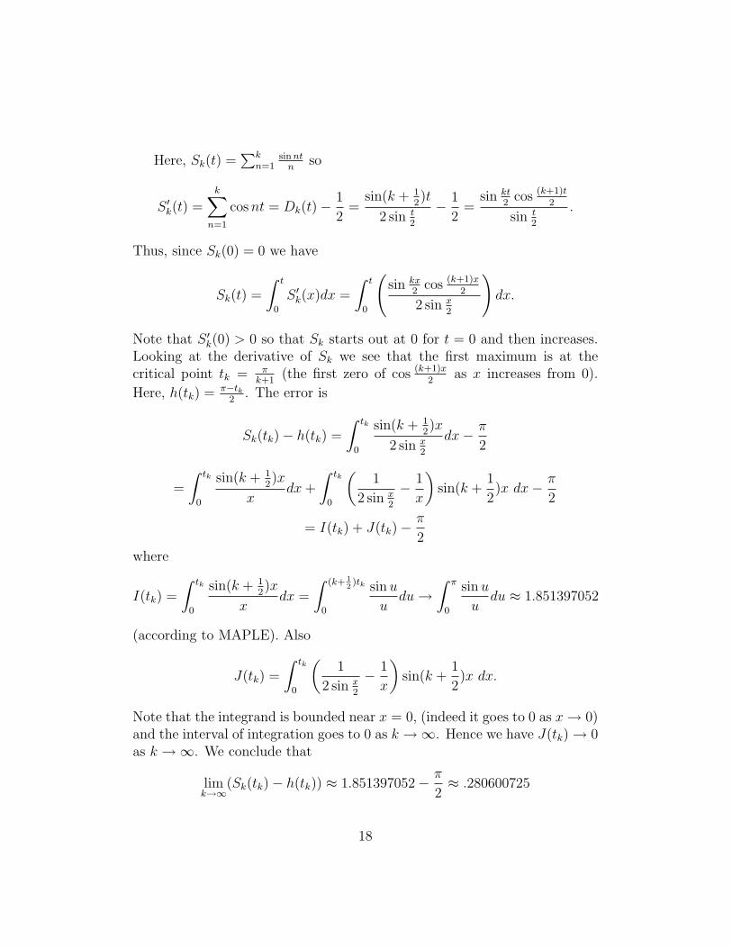
Here, Sk(t) =∑k

n=1sinntn

so

S ′k(t) =k∑

n=1

cosnt = Dk(t)−1

2=

sin(k + 12)t

2 sin t2

− 1

2=

sin kt2

cos (k+1)t2

sin t2

.

Thus, since Sk(0) = 0 we have

Sk(t) =

∫ t

0

S ′k(x)dx =

∫ t

0

(sin kx

2cos (k+1)x

2

2 sin x2

)dx.

Note that S ′k(0) > 0 so that Sk starts out at 0 for t = 0 and then increases.Looking at the derivative of Sk we see that the first maximum is at thecritical point tk = π

k+1(the first zero of cos (k+1)x

2as x increases from 0).

Here, h(tk) = π−tk2

. The error is

Sk(tk)− h(tk) =

∫ tk

0

sin(k + 12)x

2 sin x2

dx− π

2

=

∫ tk

0

sin(k + 12)x

xdx+

∫ tk

0

(1

2 sin x2

− 1

x

)sin(k +

1

2)x dx− π

2

= I(tk) + J(tk)−π

2

where

I(tk) =

∫ tk

0

sin(k + 12)x

xdx =

∫ (k+ 12)tk

0

sinu

udu→

∫ π

0

sinu

udu ≈ 1.851397052

(according to MAPLE). Also

J(tk) =

∫ tk

0

(1

2 sin x2

− 1

x

)sin(k +

1

2)x dx.

Note that the integrand is bounded near x = 0, (indeed it goes to 0 as x→ 0)and the interval of integration goes to 0 as k →∞. Hence we have J(tk)→ 0as k →∞. We conclude that

limk→∞

(Sk(tk)− h(tk)) ≈ 1.851397052− π

2≈ .280600725

18

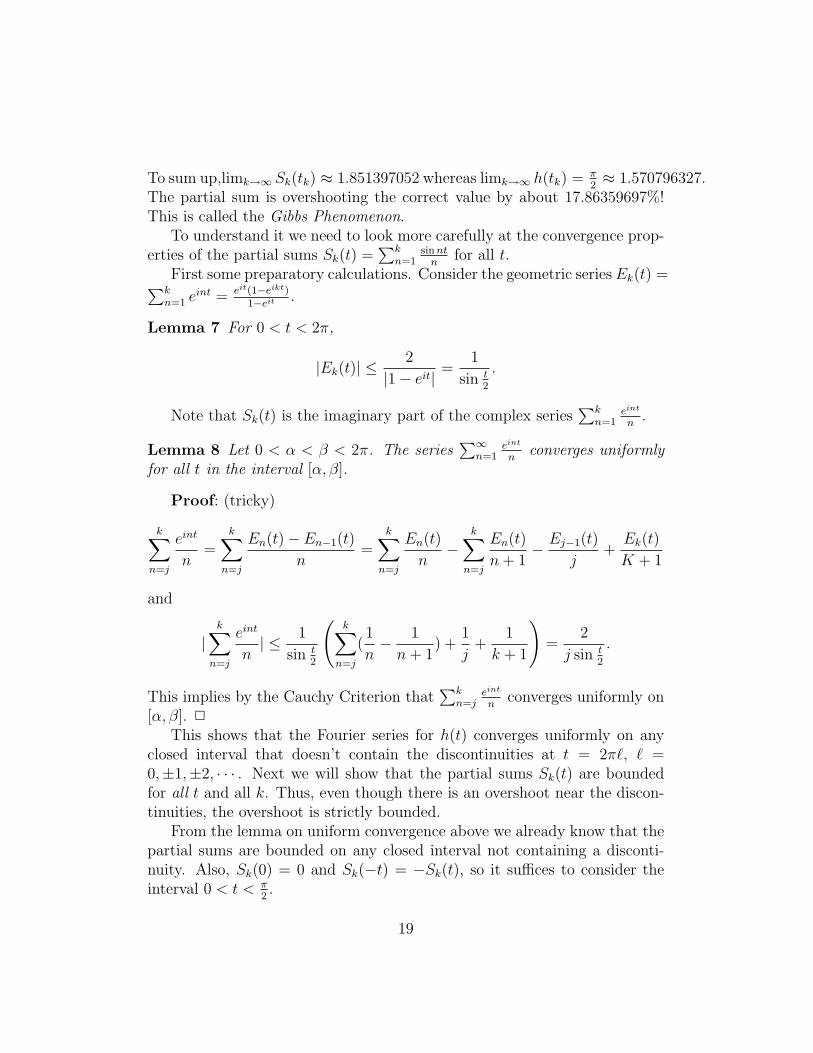
To sum up,limk→∞ Sk(tk) ≈ 1.851397052 whereas limk→∞ h(tk) = π2≈ 1.570796327.

The partial sum is overshooting the correct value by about 17.86359697%!This is called the Gibbs Phenomenon.

To understand it we need to look more carefully at the convergence prop-erties of the partial sums Sk(t) =

∑kn=1

sinntn

for all t.First some preparatory calculations. Consider the geometric series Ek(t) =∑kn=1 e

int = eit(1−eikt)1−eit .

Lemma 7 For 0 < t < 2π,

|Ek(t)| ≤2

|1− eit|=

1

sin t2

.

Note that Sk(t) is the imaginary part of the complex series∑k

n=1eint

n.

Lemma 8 Let 0 < α < β < 2π. The series∑∞

n=1eint

nconverges uniformly

for all t in the interval [α, β].

Proof: (tricky)

k∑n=j

eint

n=

k∑n=j

En(t)− En−1(t)

n=

k∑n=j

En(t)

n−

k∑n=j

En(t)

n+ 1− Ej−1(t)

j+Ek(t)

K + 1

and

|k∑n=j

eint

n| ≤ 1

sin t2

(k∑n=j

(1

n− 1

n+ 1) +

1

j+

1

k + 1

)=

2

j sin t2

.

This implies by the Cauchy Criterion that∑k

n=jeint

nconverges uniformly on

[α, β]. 2

This shows that the Fourier series for h(t) converges uniformly on anyclosed interval that doesn’t contain the discontinuities at t = 2π`, ` =0,±1,±2, · · · . Next we will show that the partial sums Sk(t) are boundedfor all t and all k. Thus, even though there is an overshoot near the discon-tinuities, the overshoot is strictly bounded.

From the lemma on uniform convergence above we already know that thepartial sums are bounded on any closed interval not containing a disconti-nuity. Also, Sk(0) = 0 and Sk(−t) = −Sk(t), so it suffices to consider theinterval 0 < t < π

2.

19

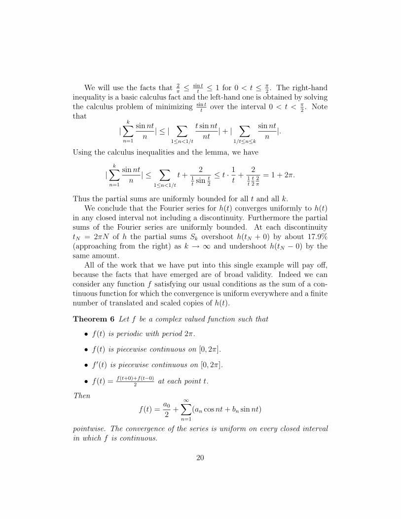
We will use the facts that 2π≤ sin t

t≤ 1 for 0 < t ≤ π

2. The right-hand

inequality is a basic calculus fact and the left-hand one is obtained by solvingthe calculus problem of minimizing sin t

tover the interval 0 < t < π

2. Note

that

|k∑

n=1

sinnt

n| ≤ |

∑1≤n<1/t

t sinnt

nt|+ |

∑1/t≤n≤k

sinnt

n|.

Using the calculus inequalities and the lemma, we have

|k∑

n=1

sinnt

n| ≤

∑1≤n<1/t

t+2

1t

sin t2

≤ t · 1

t+

21tt2

2π

= 1 + 2π.

Thus the partial sums are uniformly bounded for all t and all k.We conclude that the Fourier series for h(t) converges uniformly to h(t)

in any closed interval not including a discontinuity. Furthermore the partialsums of the Fourier series are uniformly bounded. At each discontinuitytN = 2πN of h the partial sums Sk overshoot h(tN + 0) by about 17.9%(approaching from the right) as k → ∞ and undershoot h(tN − 0) by thesame amount.

All of the work that we have put into this single example will pay off,because the facts that have emerged are of broad validity. Indeed we canconsider any function f satisfying our usual conditions as the sum of a con-tinuous function for which the convergence is uniform everywhere and a finitenumber of translated and scaled copies of h(t).

Theorem 6 Let f be a complex valued function such that




• f(t) = f(t+0)+f(t−0)2

at each point t.

Then

f(t) =a0

2+∞∑n=1


pointwise. The convergence of the series is uniform on every closed intervalin which f is continuous.

20

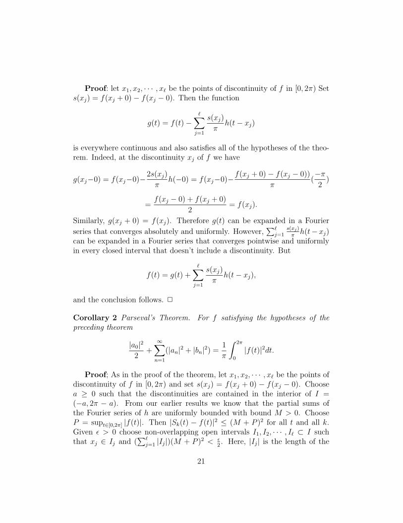
Proof: let x1, x2, · · · , x` be the points of discontinuity of f in [0, 2π) Sets(xj) = f(xj + 0)− f(xj − 0). Then the function

g(t) = f(t)−∑j=1

s(xj)

πh(t− xj)

is everywhere continuous and also satisfies all of the hypotheses of the theo-rem. Indeed, at the discontinuity xj of f we have

g(xj−0) = f(xj−0)−2s(xj)

πh(−0) = f(xj−0)−f(xj + 0)− f(xj − 0))

π(−π2

)

=f(xj − 0) + f(xj + 0)

2= f(xj).

Similarly, g(xj + 0) = f(xj). Therefore g(t) can be expanded in a Fourier

series that converges absolutely and uniformly. However,∑`

j=1s(xj)

πh(t−xj)

can be expanded in a Fourier series that converges pointwise and uniformlyin every closed interval that doesn’t include a discontinuity. But

f(t) = g(t) +∑j=1

s(xj)

πh(t− xj),

and the conclusion follows. 2

Corollary 2 Parseval’s Theorem. For f satisfying the hypotheses of thepreceding theorem

|a0|2

2+∞∑n=1

(|an|2 + |bn|2) =1

π

∫ 2π

0

|f(t)|2dt.

Proof; As in the proof of the theorem, let x1, x2, · · · , x` be the points ofdiscontinuity of f in [0, 2π) and set s(xj) = f(xj + 0) − f(xj − 0). Choosea ≥ 0 such that the discontinuities are contained in the interior of I =(−a, 2π − a). From our earlier results we know that the partial sums ofthe Fourier series of h are uniformly bounded with bound M > 0. ChooseP = supt∈[0,2π] |f(t)|. Then |Sk(t) − f(t)|2 ≤ (M + P )2 for all t and all k.Given ε > 0 choose non-overlapping open intervals I1, I2, · · · , I` ⊂ I suchthat xj ∈ Ij and (

∑`j=1 |Ij|)(M + P )2 < ε

2. Here, |Ij| is the length of the

21

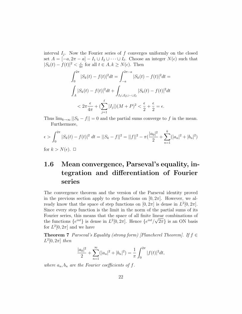
interval Ij. Now the Fourier series of f converges uniformly on the closedset A = [−a, 2π − a] − I1 ∪ I2 ∪ · · · ∪ I`. Choose an integer N(ε) such that|Sk(t)− f(t)|2 < ε

4πfor all t ∈ A, k ≥ N(ε). Then∫ 2π

0

|Sk(t)− f(t)|2dt =

∫ 2π−a

−a|Sk(t)− f(t)|2dt =∫

A

|Sk(t)− f(t)|2dt+

∫I1∪I2∪···∪I`

|Sk(t)− f(t)|2dt

< 2πε

4π+ (∑j=1

|Ij|)(M + P )2 <ε

2+ε

2= ε.

Thus limk→∞ ||Sk − f || = 0 and the partial sums converge to f in the mean.Furthermore,

ε >

∫ 2π

0

|Sk(t)− f(t)|2 dt = ||Sk − f ||2 = ||f ||2 − π(|a0|2

2+

k∑n=1

(|an|2 + |bn|2)

for k > N(ε). 2

1.6 Mean convergence, Parseval’s equality, in-

tegration and differentiation of Fourier

series

The convergence theorem and the version of the Parseval identity provedin the previous section apply to step functions on [0, 2π]. However, we al-ready know that the space of step functions on [0, 2π] is dense in L2[0, 2π].Since every step function is the limit in the norm of the partial sums of itsFourier series, this means that the space of all finite linear combinations ofthe functions {eint} is dense in L2[0, 2π]. Hence {eint/

√2π} is an ON basis

for L2[0, 2π] and we have

Theorem 7 Parseval’s Equality (strong form) [Plancherel Theorem]. If f ∈L2[0, 2π] then

|a0|2

2+∞∑n=1

(|an|2 + |bn|2) =1

π

∫ 2π

0

|f(t)|2dt,

where an, bn are the Fourier coefficients of f .

22

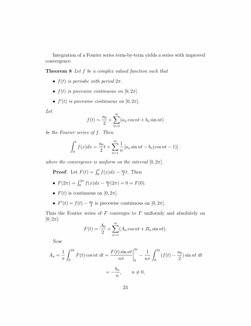
Integration of a Fourier series term-by-term yields a series with improvedconvergence.





Let

f(t) ∼ a0

2+∞∑n=1


be the Fourier series of f . Then∫ t

0

f(x)dx =a0

2t+

∞∑n=1

1

n[an sinnt− bn(cosnt− 1)] .

where the convergence is uniform on the interval [0, 2π].

Proof: Let F (t) =∫ t

0f(x)dx− a0

2t. Then

• F (2π) =∫ 2π

0f(x)dx− a0

2(2π) = 0 = F (0).

• F (t) is continuous on [0, 2π].

• F ′(t) = f(t)− a0

2is piecewise continuous on [0, 2π].

Thus the Fourier series of F converges to F uniformly and absolutely on[0, 2π]:

F (t) =A0

2+∞∑n=1

(An cosnt+Bn sinnt).

Now

An =1

π

∫ 2π

0

F (t) cosnt dt =F (t) sinnt

nπ

∣∣∣∣2π0

− 1

nπ

∫ 2π

0

(f(t)− a0

2) sinnt dt

= −bnn, n 6= 0,

23

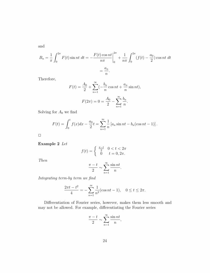
and

Bn =1

π

∫ 2π

0

F (t) sinnt dt = −F (t) cosnt

nπ

∣∣∣∣2π0

+1

nπ

∫ 2π

0

(f(t)− a0

2) cosnt dt

=ann.

Therefore,

F (t) =A0

2+∞∑n=1

(−bnn

cosnt+ann

sinnt),

F (2π) = 0 =A0

2−∞∑n=1

bnn.

Solving for A0 we find

F (t) =

∫ t

0

f(x)dx− a0

2t =

∞∑n=1

1

n[an sinnt− bn(cosnt− 1)] .

2

Example 2 Let

f(t) =

{π−t2

0 < t < 2π0 t = 0, 2π.

Thenπ − t

2∼

∞∑n=1

sinnt

n.

Integrating term-by term we find

2πt− t2

4= −

∞∑n=1

1

n2(cosnt− 1), 0 ≤ t ≤ 2π.

Differentiation of Fourier series, however, makes them less smooth andmay not be allowed. For example, differentiating the Fourier series

π − t2∼

∞∑n=1

sinnt

n,

24

formally term-by term we get

−1

2∼

∞∑n=1

cosnt,

which doesn’t converge on [0, 2π]. In fact it can’t possible be a Fourier seriesfor an element of L2[0, 2π]. (Why?)

If f is sufficiently smooth and periodic it is OK to differentiate term-by-term to get a new Fourier series.



• f(t) is continuous on [0, 2π].


• f ′′(t) is piecewise continuous on [0, 2π].

Let

f(t) =a0

2+∞∑n=1


be the Fourier series of f . Then at each point t ∈ [0, 2π] where f ′′(t) existswe have

f ′(t) =∞∑n=1

n [−an sinnt+ bn cosnt] .

Proof: By the Fourier convergence theorem the Fourier series of f ′ con-verges to f ′(t0+0)+f ′(t0−0)

2at each point t0. If f ′′(t0) exists at the point then

the Fourier series converges to f ′(t0), where

f ′(t) ∼ A0

2+∞∑n=1

(An cosnt+Bn sinnt).

Now

An =1

π

∫ 2π

0

f ′(t) cosnt dt =f(t) cosnt

π

∣∣∣∣2π0

+n

π

∫ 2π

0

f(t) sinnt dt

= nbn,

25

A0 = 1π

∫ 2π

0f ′(t)dt = 1

π(f(2π)− f(0)) = 0 (where, if necessary, we adjust the

interval of length 2π so that f ′ is continuous at the endpoints) and

Bn =1

π

∫ 2π

0

f ′(t) sinnt dt =f(t) sinnt

π

∣∣∣∣2π0

− n

π

∫ 2π

0

f(t) cosnt dt

= −nan.Therefore,

f ′(t) ∼∞∑n=1

n(bn cosnt− an sinnt).

2

Note the importance of the requirement in the theorem that f is con-tinuous everywhere and periodic, so that the boundary terms vanish in theintegration by parts formulas for An and Bn. Thus it is OK to differentiatethe Fourier series

f(t) =2πt− t2

4− π2

6= −

∞∑n=1

1

n2cosnt, 0 ≤ t ≤ 2π

term-by term, where f(0) = f(2π), to get

f ′(t) =π − t

2∼

∞∑n=1

sinnt

n.

However, even though f ′(t) is infinitely differentiable for 0 < t < 2π we havef ′(0) 6= f ′(2π), so we cannot differentiate the series again.

1.7 Arithmetic summability and Fejer’s the-

orem

We know that the kth partial sum of the Fourier series of a square integrablefunction f :

Sk(t) =a0

2+

k∑n=1


is the trigonometric polynomial of order k that best approximates f in theHilbert space sense. However, the limit of the partial sums

S(t) = limk→∞

Sk(t),

26

doesn’t necessarily converge pointwise. We have proved pointwise conver-gence for piecewise smooth functions, but if, say, all we know is that f iscontinuous then pointwise convergence is much harder to establish. Indeedthere are examples of continuous functions whose Fourier series diverges atuncountably many points. Furthermore we have seen that at points of dis-continuity the Gibbs phenomenon occurs and the partial sums overshootthe function values. In this section we will look at another way to recap-ture f(t) from its Fourier coefficients, by Cesaro sums (arithmetic means).This method is surprisingly simple, gives uniform convergence for continuousfunctions f(t) and avoids most of the Gibbs phenomena difficulties.

The basic idea is to use the arithmetic means of the partial sums toapproximate f . Recall that the kth partial sum of f(t) is defined by

Sk(t) =1

2π

∫ 2π

0

f(x)dx +

1

π

k∑n=1

(∫ 2π

0

f(x) cosnx dx cosnt+

∫ 2π

0

f(x) sinnx dx sinnt

),

so

Sk(t) =1

π

∫ 2π

0

[1

2+

k∑n=1

(cosnx cosnt+ sinnx sinnt

]f(x)dx

=1

π

∫ 2π

0

[1

2+

k∑n=1

cos[n(t− x)]

]f(x)dx

=1

π

∫ 2π

0

Dk(t− x)f(x)dx.

where the kernel Dk(t) = 12

+∑k

n=1 cosnt = −12

+∑k

m=0 cosmt. Further,

Dk(t) =cos kt− cos(k + 1)t

4 sin2 t2

=sin(k + 1

2)t

2 sin t2

.

Rather than use the partial sums Sk(t) to approximate f(t) we use thearithmetic means σk(t) of these partial sums:

σk(t) =S0(t) + S1(t) + · · ·+ Sk−1(t)

k, k = 1, 2, · · · . (1.7.12)

27

Then we have

σk(t) =1

kπ

k−1∑j=0

∫ 2π

0

Dj(t− x)f(x)dx =

∫ 2π

0

[1

kπ

k−1∑j=0

Dj(t− x)

]f(x)dx

=1

π

∫ 2π

0

Fk(t− x)f(x)dx (1.7.13)

where

Fk(t) =1

k

k−1∑j=0

Dj(t) =1

k

k−1∑j=0

sin(j + 12)t

2 sin t2

.

Lemma 9

Fk(t) =1

k

(sin kt/2

sin t/2

)2

.

Proof: Using the geometric series, we have

k−1∑j=0

ei(j+12)t = ei

t2eikt − 1

eit − 1= ei

kt2

sin kt2

sin t2

.

Taking the imaginary part of this identity we find

Fk(t) =1

k sin t2

k−1∑j=0

sin(j +1

2)t =

1

k

(sin kt/2

sin t/2

)2

.

2

Note that F has the properties:

• Fk(t) = Fk(t+ 2π)

• Fk(−t) = Fk(t)

• Fk(t) is defined and differentiable for all t and Fk(0) = k

• Fk(t) ≥ 0.

From these properties it follows that the integrand of (1.7.13) is a 2π-periodicfunction of x, so that we can take the integral over any full 2π-period. Finally,we can change variables and divide up the integral, in analogy with our studyof the Fourier kernel Dk(t), and obtain the following simple expression forthe arithmetic means:

28

Lemma 10

σk(t) =2

kπ

∫ π/2

0

f(t+ 2x) + f(t− 2x)

2

(sin kx

sinx

)2

dx.

Exercise 7 Derive Lemma 10 from expression(1.7.13) and Lemma 9.

Lemma 112

kπ

∫ π/2

0

(sin kx

sinx

)2

dx = 1.

Proof: Let f(t) ≡ 1 for all t. Then σk(t) ≡ 1 for all k and t. Substitutinginto the expression from lemma 10 we obtain the result. 2

Theorem 10 (Fejer) Suppose f(t) ∈ L1[0, 2π], periodic with period 2π andlet

σ(t) = limx→0+

f(t+ x) + f(t− x)

2=f(t+ 0) + f(t− 0)

2

whenever the limit exists. For any t such that σ(t) is defined we have

limk→∞

σk(t) = σ(t) =f(t+ 0) + f(t− 0)

2.

Proof: From lemmas 10 and 11 we have

σk(t)− σ(t) =2

kπ

∫ π/2

0

[f(t+ 2x) + f(t− 2x)

2− σ(t)

](sin kx

sinx

)2

dx.

For any t for which σ(t) is defined, let Gt(x) = f(t+2x)+f(t−2x)2

− σ(t). ThenGt(x) → 0 as t → 0 through positive values. Thus, given ε > 0 there is aδ < π/2 such that |Gt(x)| < ε/2 whenever 0 < x ≤ δ. We have

σk(t)− σ(t) =2

kπ

∫ δ

0

Gt(x)

(sin kx

sinx

)2

dx+2

kπ

∫ π/2

δ

Gt(x)

(sin kx

sinx

)2

dx.

Now ∣∣∣∣∣ 2

kπ

∫ δ

0

Gt(x)

(sin kx

sinx

)2

dx

∣∣∣∣∣ ≤ ε

kπ

∫ π/2

0

(sin kx

sinx

)2

dx =ε

2

29

and∣∣∣∣∣ 2

kπ

∫ π/2

δ

Gt(x)

(sin kx

sinx

)2

dx

∣∣∣∣∣ ≤ 2

kπ sin2 δ

∫ π/2

δ

|Gt(x)|dx ≤ 2I

kπ sin2 δ,

where I =∫ π/2

0|Gt(x)|dx. This last integral exists because F is in L1. Now

choose K so large that 2I/(Nπ sin2 δ) < ε/2. Then if k ≥ K we have

|σk(t)−σ(t)| ≤

∣∣∣∣∣ 2

kπ

∫ δ

0

Gt(x)

(sin kx

sinx

)2

dx

∣∣∣∣∣+∣∣∣∣∣ 2

kπ

∫ π/2

δ

Gt(x)

(sin kx

sinx

)2

dx

∣∣∣∣∣ < ε.

2

Corollary 3 Suppose f(t) satisfies the hypotheses of the theorem and alsois continuous on the closed interval [a, b]. Then the sequence of arithmeticmeans σk(t) converges uniformly to f(t) on [a, b].

Proof: If f is continuous on the closed bounded interval [a, b] then it isuniformly continuous on that interval and the function Gt is bounded on [a, b]with upper bound M , independent of t. Furthermore one can determine theδ in the preceding theorem so that |Gt(x)| < ε/2 whenever 0 < x ≤ δ anduniformly for all t ∈ [a, b]. Thus we can conclude that σk → σ, uniformly on[a, b]. Since f is continuous on [a, b] we have σ(t) = f(t) for all t ∈ [a, b]. 2

Corollary 4 (Weierstrass approximation theorem) Suppose f(t) is real andcontinuous on the closed interval [a, b]. Then for any ε > 0 there exists apolynomial p(t) such that

|f(t)− p(t)| < ε

for every t ∈ [a, b].

Sketch of Proof: Using the methods of Section 1.3 we can find a lin-ear transformation to map [a, b] one-to-one on a closed subinterval [a′, b′] of[0, 2π], such that 0 < a′ < b′ < 2π. This transformation will take polyno-mials in t to polynomials. Thus, without loss of generality, we can assume0 < a < b < 2π. Let g(t) = f(t) for a ≤ t ≤ b and define g(t) outside thatinterval so that it is continuous at T = a, b and is periodic with period 2π.Then from the first corollary to Fejer’s theorem, given an ε > 0 there is aninteger N and

30

arithmetic sum

σ(t) =A0

2+

N∑j=1

(Aj cos jt+Bj sin jt)

such that |f(t) − σ(t)| = |g(t) − σ(t)| < ε2

for a ≤ t ≤ b. Now σ(t) isa trigonometric polynomial and it determines a poser series expansion int about the origin that converges uniformly on every finite interval. Thepartial sums of this power series determine a series of polynomials {pn(t)} oforder n such that pn → σ uniformly on [a, b], Thus there is an M such that|σ(t)− pM(t)| < ε

2for all t ∈ [a, b]. Thus

|f(t)− pM(t)| ≤ |f(t)− σ(t)|+ |σ(t)− pM(t)| < ε

for all t ∈ [a, b]. 2

This important result implies not only that a continuous function on abounded interval can be approximated uniformly by a polynomial functionbut also (since the convergence is uniform) that continuous functions onbounded domains can be approximated with arbitrary accuracy in the L2

norm on that domain. Indeed the space of polynomials is dense in thatHilbert space.

Another important offshoot of approximation by arithmetic sums is thatthe Gibbs phenomenon doesn’t occur. This follows easily from the nextresult.

Lemma 12 Suppose the 2π-periodic function f(t) ∈ L2[−π, π] is bounded,with M = supt∈[−π,π] |f(t)|. Then |σn(t)| ≤M for all t.

Proof: From (1.7.13) and (10) we have

|σk(t)| ≤1

2kπ

∫ 2π

0

|f(t+x)|(

sin kx/2

sinx/2

)2

dx ≤ M

2kπ

∫ 2π

0

(sin kx/2

sinx/2

)2

dx = M.

Q.E.D.Now consider the example which has been our prototype for the Gibbs

phenomenon:

h(t) =

0, t = 0π−t2, 0 < t < 2π

0, t = 2π.

31

and h(t+ 2π) = h(t). Here the ordinary Fourier series gives

π − t2

=∞∑n=1

sinnt

n, 0 < t < 2π.

and this series exhibits the Gibbs phenomenon near the simple discontinuitiesat integer multiples of 2π. Furthermore the supremum of |h(t)| is π/2 andit approaches the values ±π/2 near the discontinuities. However, the lemmashows that |σ(t)| < π/2 for all n and t. Thus the arithmetic sums neverovershoot or undershoot as t approaches the discontinuities, so there is noGibbs phenomenon in the arithmetic series for this example.

In fact, the example is universal; there is no Gibbs phenomenon for arith-metic sums. To see this, we can mimic the proof of Theorem 6. This thenshows that the arithmetic sums for all piecewise smooth functions convergeuniformly except in arbitrarily small neighborhoods of the discontinuitiesof these functions. In the neighborhood of each discontinuity the arithmeticsums behave exactly as does the series for h(t). Thus there is no overshootingor undershooting.

Remark 1 The pointwise convergence criteria for the arithmetic means aremuch more general (and the proofs of the theorems are simpler) than forthe case of ordinary Fourier series. Further, they provide a means of gettingaround the most serious problems caused by the Gibbs phenomenon. The tech-nical reason for this is that the kernel function Fk(t) is nonnegative. Whydon’t we drop ordinary Fourier series and just use the arithmetic means?There are a number of reasons, one being that the arithmetic means σk(t)arenot the best L2 approximations for order k, whereas the Sk(t) are the best L2

approximations. There is no Parseval theorem for arithmetic means. Fur-ther, once the approximation Sk(t) is computed for ordinary Fourier series,in order to get the next level of approximation one needs only to compute twomore constants:

Sk+1(t) = Sk(t) + ak+1 cos(k + 1)t+ bk+1 sin(k + 1)t.

However, for the arithmetic means, in order to update σk(t) to σk+1(t) onemust recompute ALL of the expansion coefficients. This is a serious practicaldifficulty.

32

1.8 Additional Exercises

Exercise 8 (1) Let X be the Eucldean space Cn of all n ≥ 1 tuples (x1, .., xn)of complex numbers. For x, y ∈ X, define

(x.y) =n∑j=1

xjyj

where z denotes the complex conjugate of z ∈ C. Show that (; .; ) sat-isfies the properties of positivity, homogeneity and linearity and withsymmetry, replaced by compex symmetry (x, y) = (x, y). Hence (; .; )defines a compex inner product on X.

(2) Define ||x|| =√

(x, x) for x ∈ X and verify directly that (1) ||; || is anorm on X, (2) that the Cauchy-Schwartz inequality

|(x, y)| ≤ ||x||||y||

holds on X and (3) that the parallelogram law

||x+ y||2 + ||x− y||2 = 2||x||2 + 2||y||2

holds on X.

Exercise 9 Let X b the space R[−π, π] with inner product

(f, g) =1

π

∫ π

−πf(x)g(x)dx.

Show that the sequence of functions{1√2, cos(x), sin(x), cos(2x), sin(2x), .....

}is an orthonormal sequence in X.

Exercise 10 Let X = R[−1, 1] with inner product

(f, g) =

∫ 1

−1

f(x)g(x)dx.

33

Find polynomials P0, P1, P2 of degree 0, 1, 2 respectively such that for j, k =0, 1, 2

(Pj, Pk) = δj,k =

{0, j 6= k1, j = k

Hint: First find P0(x) = c satisfying (P0, P0) = 1. Next, find P1(x) = a+ bxsatisfying

(P1, P0) = 0, (P1, P1) = 1.

Next, find P2(x) = d+ ex+ fx2 satisfying

(P2, P0) = (P2, P1) = 0, (P2, P2) = 1.

This procedure can be continued indefinitely and is called the Gram-Schmidtprocess.

Exercise 11 Let f(x) = x, x ∈ [−π, π].

(a) Show that f(x) has the Fourier series

∞∑n=1

2

n(−1)n−1 sin(nx).

(b) Let α > 0. Show that f(x) = exp(αx), x ∈ [−π, π] has the Fourierseries (

eαπ − e−απ

π

)(1

2α+∞∑k=1

(−1)kα cos(kx)− k sin(kx)

α2 + k2

).

(c) Let α be any real number other than an integer. Let f(x) = cos(αx), x ∈[−π, π]. Show that f has a Fourier series

sin(απ)

απ+

1

π

∞∑n=1

[sin(α + n)π

α + n+ +

sin(α− n)π

α− n

]cos(nx).

(d) Find the Fourier series of f(x) = −α sin(αx), x ∈ [−π, π]. Do younotice any relationship to that in (c)?

(e) Find the Fourier series of f(x) = |x|, x ∈ [−π, π].

34

(f) Find the Fourier series of

f(x) = sign(x) =

−1, x < 00, x = 01, x > 0

Do you notice any relationship to that in (e)?

Exercise 12 Show that if f ∈ R[−π, π] is odd, then all its Fourier cosinecoefficients an = 0, n ≥ 0 so f has a Fourier series

∑∞n=1 bn sin(nx). Like-

wise, if f is even, show that all its Fourier sine coeffcients bn = 0, n ≥ 0 andf has a Fourier series a0/2 +

∑∞n=1 an cos(nx).

Exercise 13 By substituting special values of x in convergent Fourier series,we can often deduce interesting series expansions for various numbers, or justfind the sum of important series.

(a) Use the Fourier series for f(x) = x2 to show that

∞∑n=1

(−1)n−1

n2=π2

12.

(b) Prove that the Fourier series for f(x) = x converges in (−π, π) andhence that

∞∑l=0

(−1)l

2l + 1=π

4.

(c) Show that the Fourier series of f(x) = exp(αx), x ∈ [−π, π) converges

in [−π, π) to exp(αx) and at x = π to exp(απ)+exp(−απ)2

. Hence showthat

απ

tanh(απ)= 1 +

∞∑k=1

2α2

k2 + α2.

(d) Show that

π

4=

1

2+∞∑n=1

(−1)n−1

4n2 − 1.

35

(e) Show that∞∑l=0

1

(2l + 1)2=π2

8.

Exercise 14 Let f ∈ R[−π, π] be 2π periodic and let σn, n = 0, 1, 3, ... de-note its Fejer means. Show that

max {|σn(x)| : x ∈ [−π, π]} ≤ sup {|f(x)| : x ∈ [−π, π]} .

Exercise 15 The following exercise concerns an extension of Parsevals for-mula to R[−π, π]. Consider R[−π, π] with inner product

(f, g) =1

π

∫ π

−πf(x)g(x)dx, f, g ∈ R[−π, π]

and ||f || =√

(f, f). Fix f ∈ R[−π, π] and ε > 0.

(a) Because f ∈ R[−π, π], choose a partition

−π = x0 < x1 < x2 < ... < xn = π

such that if

Mj := sup {f(x) : x ∈ [xj−1, xj]} , mj := inf {f(x) : x ∈ [xj−1, xj]} , j = 1, ..., n

thenn∑j=1

(Mj −mj)(xj − xj−1) < ε.

Now define g(x) := Mj, x ∈ [xj−1, xj), 1 ≤ j ≤ n and g(b) arbitrarily.Show that ∫ π

−π|f(x)− g(x)|dx < ε.

(b) Show that there is a continuous function h : [−π, π]→ R such that∫ π

−π|g(x)− h(x))|dx < ε

and|h(x)| ≤M = max {|M1|, ..., |Mn|} , x ∈ [−π, π].

Hint: Sketch the graph of g and modify g near each xj.

36

(c) Deduce that ∫ π

−π|f(x)− h(x))|dx < 2ε

and

||f − h||2 =1

π

∫ π

−π|f(x)− h(x))|2dx < 4ε

πM∗

where M∗ = sup {|f(x)| : x ∈ [a, b)}.

(d) Deduce that given any f ∈ R[−π, π] and δ > 0, we can find a continuoush : [−π, π]→ R such that ||f − h|| < δ/2 and hence, that there exists atrigonometric polynomial t such that

||f − t|| < δ.

(e) Let Sn be the sequence of partial sums of the Fourier series of f . Showthat

limn→∞

||f − Sn|| = 0.

(f) If (an) and (bn) are the Fourier series coefficients of f , deduce that

a20/2 +

∞∑n=1

(a2n + b2n) =

1

π

∫ π

−πf 2(x)dx.

This is Parseval’s identity for R[−π, π].

Exercise 16 By applying Parsevals identity to suitable Fourier series:

(a) Show that∞∑n=1

1

n2=π2

6.

(b) Show that∞∑n=1

1

n4=π4

90.

(c) Evaluate∞∑n=1

1

α2 + n2, α > 0.

37

(d) Show that∞∑l=0

1

(2l + 1)4=π4

96.

Exercise 17 Is∞∑n=1

cos(nx)

n1/2

the Fourier series of some f ∈ R[−π, π]? The same question for the series

∞∑n=1

cos(nx)

log(n+ 2).

Exercise 18 Show that

Π∞n=2

(1− 2

n(n+ 1)

)= 1/3.


Π∞n=1

(1 +

6

(n+ 1)(2n+ 9)

)= 21/8.


Π∞n=0(1 + x2n

) =1

1− x, |x| < 1.

Hint:(Multiply the partial products by 1− x.)

Exercise 21 Let a, b ∈ C and suppose that they are not negative integers.Show that

Π∞n=1

(1 +

a− b− 1

(n+ a)(n+ b)

)=

a

b+ 1.

Hint: Note that (b+1)(a−1)

= ab+ a− b− 1, (b+ 1) + (a− 1) = a+ b.

Exercise 22 Is Π∞n=0(1 + n−1) convergent?

Exercise 23 Prove the inequality

0 ≤ eu − 1 ≤ 3u, u ∈ (0, 1)

and deduce that Π∞n=1

(1 + 1

n[e1/n − 1]

)converges.

38

Exercise 24 The Euler Mascheroni Constant. Let

Hn =n∑k=1

1

k, n ≥ 1.

Show that 1/k ≥ 1/x, x ∈ [k, k + 1] and hence that

1/k ≥∫ k+1

k

1/xdx.

Deduce that

Hn ≥∫ n+1

1

1/xdx = log(n+ 1)

and that

[Hn − log(n+ 1)]− [Hn − log n] =1

n+ 1+ log

(1− 1

n+ 1

)= −

∞∑k=2

(1

n+ 1

)k/k < 0.

Deduce that Hn− log n decreases as n increases and thus has a non-negativelimit γ, called the Euler-Mascheroni constant and with value approximately0.5772... not known to be either rational or irrational. Finally show that

Πnk=1(1 + 1/k)e−1/k = Πn

k=1(1 + 1/k)Πnk=1e

−1/k =n+ 1

nexp(−(Hn − log n)).

Deduce thatΠ∞k=1(1 + 1/k)e−1/k = e−γ.

Many functions have nice infinite product expansions which can be de-rived from first principles. The following examples illustrate some of thesenice expansions.

Exercise 25 The aim of this exercise, is to establish Euler’s reflection for-mula:

Γ(x)Γ(1− x) =π

sin(πx), Re(x) > 0.

39

Step 1: Set y = 1− x, 0 < x < 1 in the integral∫ ∞0

sx−1

(1 + s)x+yds =

Γ(x)Γ(y)

Γ(x+ y)

to obtain

Γ(x)Γ(1− x) =

∫ ∞0

tx−1

1 + tdt.

Step 2: Let now C consist of 2 circles about the origin of radii R and εrespectively which are joined alog the negative real axis from R to −ε. Showthat ∫

C

zx−1

1− zdz = −2iπ

where zx−1 takes its principle value.

Now let us write,

−2iπ =

∫ π

−π

iRx exp(ixθ)

1−R exp(iθ)dθ +

∫ ε

R

tx−1 exp(ixπ)

1 + tdt

+

∫ π

−π

iεx exp(ixθ)

1− ε exp(iθ)dθ +

∫ R

ε

tx−1 exp(−ixπ)

1 + tdt.

Let R→∞ and ε→ 0+ to deduce the result for 0 < x < 1 and for Rex 0 bycontinuation.

Exercise 26 Using the previous exercise, derive the following expansions forall arguments the RHS is meaningful.

(1)sin(x) = xΠ∞j=1

(1− (x/jπ)2) .

(2)

cos(x) = Π∞j=1

(1−

(x

(j − 1/2)π

)2).

(3) Eulers product formula for the Gamma function.

xΓ(x) = Π∞n=1

[(1 + 1/n)x(1 + x/n)−1

].

40

(4) Weierstrass’s product formula for the Gamma function

(Γ(x))−1 = xexγΠ∞k=1

[(1 + x/k)e−x/k

].

Here, γ is the Euler-Mascheroni constant.

Exercise 27 Define

H(z) = Π∞n=0

(1 + azqn

1− zqn

), |q| < 1, |z| < 1, |a| < 1.

(i) Show that

H(z) = Π∞n=0

(1 +

(a+ 1)zqn

1− zqn

)converges absolutely.

(ii) Show that(1− z)H(z) = (1 + az)H(zq).

(iii) Write

H(z) =∞∑n=0

Anzn, A0 = 1.

Use (ii) to show that

(1− qn)An = (1 + aqn−1)An−1, n ≥ 1

Deduce that

An =(1 + a)(1 + aq)...(1 + aqn−1)

(1− q)(1− q2)...(1− qn), n ≥ 1.

So for |z| < 1,

1 +∞∑n=1

(1 + a)(1 + aq)...(1 + aqn−1)

(1− q)(1− q2)...(1− qn)zn = Π∞n=0

(1 + azqn

1− zqn

).

(iv) Deduce that if 0 < |b| < |a| and |zb| < 1,

1 +∞∑n=1

((b+ a)(b+ aq)...(b+ aqn−1)

(1− q)(1− q2)...(1− qn)

)zn = Π∞n=0

(1 + azqn

1− bzqn

).

41

Exercise 28 Let D(n) denote the number of partitions of n into distinctparts (that is, n=sum of positive integers, all different). For example, D(5) =2 as 5 = 4 + 1, 5 = 3 + 2. Show formally that

∞∑n=0

D(n)qn = Π∞j=1(1 + qj).

42

Fourier Series

Documents

Transcript of Fourier Series